A MICROMECHANICS MODEL OF THERMAL EXPANSION …

A MICROMECHANICS MODEL OF THERMAL EXPANSION

COEFFICIENT IN FIBER REINFORCED COMPOSITES

by

NITTAPON SRISUK

Presented to the Faculty of the Graduate School of

The University of Texas at Arlington in Partial Fulfillment

of the Requirements

for the Degree of

MASTER OF SCIENCE IN AEROSPACE ENGINEERING

THE UNIVERSITY OF TEXAS AT ARLINGTON

December 2010

Copyright c⃝ by NITTAPON SRISUK 2010

All Rights Reserved

ACKNOWLEDGEMENTS

I would like to acknowledge my supervising professor Dr. Wen S. Chan for his

invaluable guidance and encouragement and support that helped me throughout the

entire academic program. Without his patient and attentive guidance, this thesis

would not been possible.

Also, I would like to thank Dr. Erian Armanios and Dr. Seiichi Nomura, the

members of committee, for their comments and for taking time to serve in my thesis

committee.

I would also like to extend my appreciation to Royal Thai Air Force, especially

Directorate of Aeronautical Engineering, for providing scholarship for my study.

I also wish to thank the former students of Dr. Chan’s, Mr. Selvaraj and Dr.

Rios, for their assistance in developing ANSYS code. In addition, I would also like

to thank all of my friends for their support and encouragement.

Finally, I specially thank my parents and family for their support and encour-

agement during this study period.

November 1, 2010

iii

ABSTRACT

A MICROMECHANICS MODEL OF THERMAL EXPANSION

COEFFICIENT IN FIBER REINFORCED COMPOSITES

NITTAPON SRISUK, M.S.

The University of Texas at Arlington, 2010

Supervising Professor: Wen Chan

Fiber reinforced composites are widely used for the various applications in the

aerospace, automotive, infrastructures and sporting goods industries. The evaluations

of its mechanical and thermal properties are needed for accurate estimation of their

structural response.

In this study, a mathematical closed-form expression of unit cell model was

developed to estimate the coefficient of thermal expansion (CTE) along longitudinal

and transverse directions of unidirectional lamina. Unlike the previous models, the

present model takes into consideration of the fiber configuration and volume fraction

of each constituent in the unit cell. In addition, the model is also able to obtain the

stresses of the fiber and matrix of unit cell under the temperature environment. The

results obtained by present model was validated by ANSY finite model.

The parametric study was conducted to better understanding the effect of the

CTEs on the fiber volume fraction and fiber configuration. Comparison of the CTEs

results obtained by the rule-of-mixture (ROM) and Shaperys model as well as the

FEM was conducted. The results of longitudinal CTE are in excellent agreement

iv

among all of the models. In the transverse CTE, the present result has better agree-

ment with the FEM result than with the other models. The present results also

indicate that changing the fiber configurations does affect the transverse CTE but

not longitudinal CTE.

v

TABLE OF CONTENTS

ACKNOWLEDGEMENTS . . . . . . . . . . . . . . . . . . . . . . . . . . . . iii

ABSTRACT . . . . . . . . . . . . . . . . . . . . . . . . . . . . . . . . . . . . iv

LIST OF FIGURES . . . . . . . . . . . . . . . . . . . . . . . . . . . . . . . . viii

Chapter Page

1. INTRODUCTION . . . . . . . . . . . . . . . . . . . . . . . . . . . . . . . 1

1.1 Background . . . . . . . . . . . . . . . . . . . . . . . . . . . . . . . . 1

1.2 Objective of Research . . . . . . . . . . . . . . . . . . . . . . . . . . . 2

1.3 Outline of This Thesis . . . . . . . . . . . . . . . . . . . . . . . . . . 3

2. ANALYTICAL MODEL WITH THERMAL EXPANSION . . . . . . . . . 4

2.1 Approach of Analytical Model Development . . . . . . . . . . . . . . 5

2.2 Reduced Stiffness Matrix of Sub-layer . . . . . . . . . . . . . . . . . . 8

2.3 Laminate Stiffness and Thermal Resultant Matrices . . . . . . . . . . 17

2.4 Methods of Obtaining the Effective Properties . . . . . . . . . . . . . 24

2.5 Stresses Components due to Thermal Expansion . . . . . . . . . . . . 27

2.6 Rule-of-Mixture and Schapery’s Methods . . . . . . . . . . . . . . . . 27

3. FINITE ELEMENT ANALYSIS . . . . . . . . . . . . . . . . . . . . . . . . 30

3.1 Finite Element Model for Longitudinal Load . . . . . . . . . . . . . . 30

3.1.1 Geometric Description . . . . . . . . . . . . . . . . . . . . . . 30

3.1.2 Materials Used . . . . . . . . . . . . . . . . . . . . . . . . . . 31

3.1.3 Element Type Used . . . . . . . . . . . . . . . . . . . . . . . . 31

3.1.4 Modeling and Mesh Generation . . . . . . . . . . . . . . . . . 32

3.1.5 Boundary and Loading Conditions . . . . . . . . . . . . . . . 33

vi

3.2 Finite Element Model for Thermal Load . . . . . . . . . . . . . . . . 33


3.3 Finite Element Model for Transverse Load . . . . . . . . . . . . . . . 34

3.3.1 Geometric Description . . . . . . . . . . . . . . . . . . . . . . 34


3.4 Method of Obtaining the Effective Properties . . . . . . . . . . . . . 35

4. NUMERICAL RESULTS AND DISCUSSIONS . . . . . . . . . . . . . . . 45

4.1 Effects of Fiber Volume Fraction on Effective Properties . . . . . . . 45

4.2 Effects of Fiber Configuration on the Effective Properties . . . . . . . 49

4.2.1 Effects of Fiber Configuration in Analytical Solution . . . . . 49

4.2.2 Effects of Fiber Configurations in Finite Element Analysis . . 50

4.3 Stress Component Due to Thermal Expansion . . . . . . . . . . . . . 54

5. CONCLUSION . . . . . . . . . . . . . . . . . . . . . . . . . . . . . . . . . 57

Appendix

A. THE INTEGRALS USED IN ANALYTICAL SOLUTIONS . . . . . . . . 59

B. FEM CODES FOR ANSYS 11.0 PROGRAMS . . . . . . . . . . . . . . . 64

C. THE COMPARATIVE DATA . . . . . . . . . . . . . . . . . . . . . . . . . 76

REFERENCES . . . . . . . . . . . . . . . . . . . . . . . . . . . . . . . . . . . 83

BIOGRAPHICAL STATEMENT . . . . . . . . . . . . . . . . . . . . . . . . . 85

vii

LIST OF FIGURES

Figure Page

2.1 Microstructure and Unit Cell of Fiber Reinforced Composite . . . . . 5

2.2 Cross-Sectional Area and Geometry of Unit Cell . . . . . . . . . . . . 6

2.3 Example of Sub-layer in Unit Cell . . . . . . . . . . . . . . . . . . . . 6

3.1 Unit Cell with Circular Fiber . . . . . . . . . . . . . . . . . . . . . . . 37

3.2 Unit Cell with Elliptical Fiber . . . . . . . . . . . . . . . . . . . . . . 37

3.3 Cross-sectional Area in FEM Model with Circular Fiber . . . . . . . . 38

3.4 Cross-sectional Area in FEM Model with Elliptical Fiber . . . . . . . 38

3.5 2D-Mesh in FEM Model with Circular Fiber . . . . . . . . . . . . . . 39

3.6 2D-Mesh in FEM Model with Elliptical Fiber . . . . . . . . . . . . . . 39

3.7 3D-Mesh in FEM Model with Circular Fiber . . . . . . . . . . . . . . 40

3.8 3D-Mesh in FEM Model with Elliptical Fiber . . . . . . . . . . . . . . 40

3.9 3D-Mesh in Transverse Load Model with Circular Fiber . . . . . . . . 41

3.10 3D-Mesh in Transverse Load Model with Elliptical Fiber . . . . . . . 41

3.11 X-direction Total Strain in FEM Model with Circular Fiber . . . . . . 42

3.12 X-direction Total Strain in FEM Model with Elliptical Fiber . . . . . 42

3.13 Y-Direction Deformation in FEM Model with Circular Fiber . . . . . 43

3.14 Y-Direction Deformation in FEM Model with Elliptical Fiber . . . . . 43

3.15 X-Direction Stress in FEM Model with Circular Fiber . . . . . . . . . 44

3.16 X-Direction Stress in FEM Model with Elliptical Fiber . . . . . . . . 44

4.1 Fiber Size Varies with Fiber Volume Fraction . . . . . . . . . . . . . . 46

4.2 Longitudinal Modulus Respect with Fiber Volume Fraction . . . . . . 47

viii

4.3 Transverse Modulus Respect with Fiber Volume Fraction . . . . . . . 47

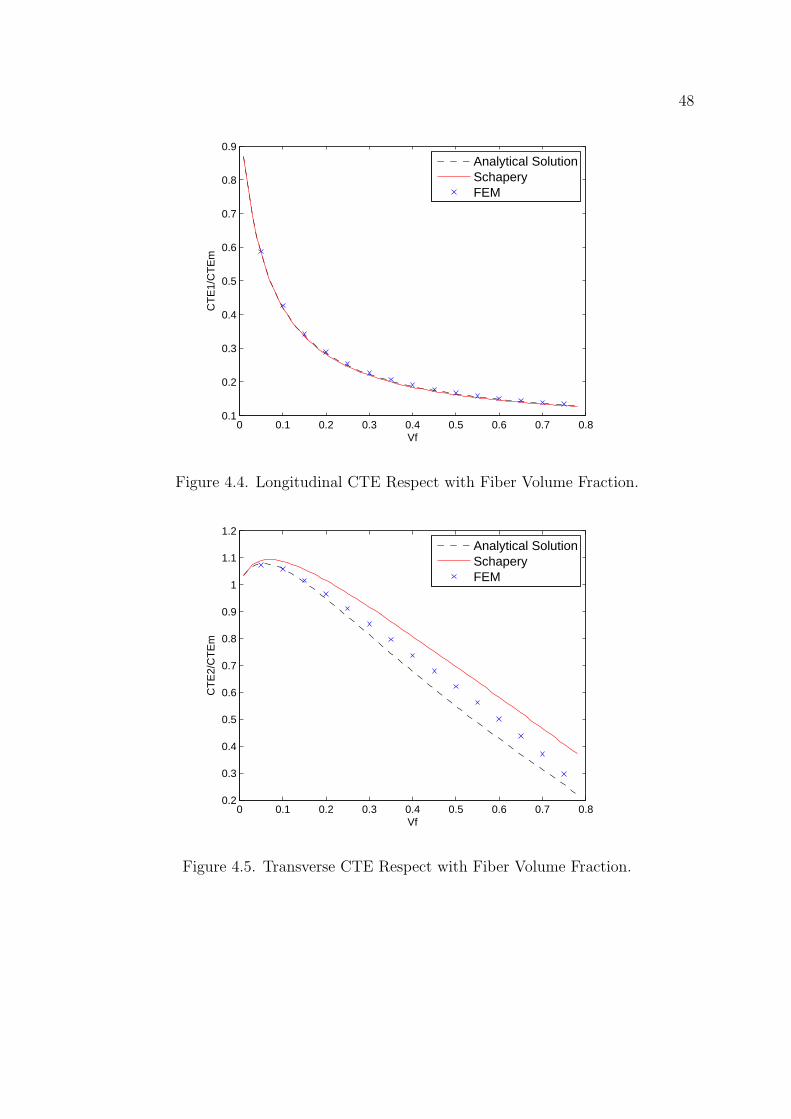
4.4 Longitudinal CTE Respect with Fiber Volume Fraction . . . . . . . . 48

4.5 Transverse CTE Respect with Fiber Volume Fraction . . . . . . . . . 48

4.6 Fiber Shape Varies with Axial Ratio . . . . . . . . . . . . . . . . . . . 49

4.7 Moduli Ratio Respect with Axial Ratio in Analytical Solution . . . . 51

4.8 Moduli Ratio Respect with Axial Ratio in FEM . . . . . . . . . . . . 51

4.9 CTE Ratio Respect with Axial Ratio in Analytical Solution . . . . . . 52

4.10 CTE Ratio Respect with Axial Ratio in FEM . . . . . . . . . . . . . 52

4.11 Moduli Ratio Respect with Axial Ratio in Both Solutions . . . . . . . 53

4.12 CTE Ratio Respect with Axial Ratio in Both Solutions . . . . . . . . 53

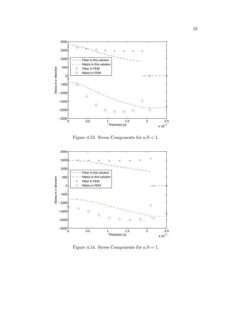
4.13 Stress Components for a/b < 1 . . . . . . . . . . . . . . . . . . . . . . 55

4.14 Stress Components for a/b = 1 . . . . . . . . . . . . . . . . . . . . . . 55

4.15 Stress Components for a/b > 1 . . . . . . . . . . . . . . . . . . . . . . 56

ix

CHAPTER 1

INTRODUCTION

1.1 Background

Structural applications of composite materials require accurate estimation of

structural response in different temperature environments. The coefficient of thermal

expansion (CTE) is the thermoelastic property that shows the response of the material

geometry when the temperature is changed. In composite materials, the CTE is more

complex than that in isotropic materials. There are three well-known methods to

evaluate the properties of fiber reinforced composite, especially the CTEs.

First of all, the CTEs and the other properties of fiber reinforced composite can

be experimentally characterized in the laboratory. The specimens of the materials

will be tested under the uniform thermal load in steady state condition. Among there,

the transverse and longitudinal CTEs were measured in the experiment of Kulkarni

and Ochoa[1]. Kia[2] also measured the CTEs from the experiments in sheet molding

compound (SMC) composites. However, the experiment will be considerably costly

and time consuming when appraising in the materials with some parameters studies

such as the fiber volume fraction and configuration. In addition, the most experiments

were focused on the effects of temperature not the volume fraction and configuration

of fiber.

Secondly, many analytical models were created for evaluating the composite

properties, includes the CTEs, in different material systems. Among them, the rule-

of-mixture (ROM) model which was based upon the linear or reciprocal linear re-

lationship of the fiber and matrix fraction to determine the properties. Schapery[3]

1

2

used energy principles to determine the longitudinal and transverse CTEs of unidirec-

tional composites. Likewise, Rosen and Hashin[4] also derived the CTEs estimation

based on thermoelastic energy principles. The transverse CTE is more complex for

prediction. Therefore, some researches only focused in the evaluation of transverse

CTE such as Tandon and Chatterjee[5]. Ishikawa, Koyama and Kobayashi[6] derived

the analytical solution and conducted the experiment to evaluate the CTEs in both

directions. Moreover, Melo and Radford[7] determined the properties, includes the

CTEs analytically and experimentally for the different angle ply of the composite

laminates. Wang and Chan[8] developed an analytical model of unit cell to evalu-

ated the stiffness of composite rod reinforced lamina. Both circular and elliptical

cross-sections of composite rods were studied. Likewise, the micromechanics model

of square array unit cell of heterogeneous materials were formed for predicting the

CTEs by Yu and Tang[9].

With the development in computer technology, the numerical solutions, es-

pecially the finite element analysis (FEA), are also employed to study the CTEs.

2D-FEM models of the square array of fiber reinforced composite with and without

cracked were created in ABAQUS program to solve both longitudinal and transverse

CTEs by Islam, Sjolind and Pramila[10]. Kulkarni and Ochoa[1] also used 2D-FEM

model of the representative volume element (RVE) of the hexagonal array of fiber re-

inforced composites to solve the CTEs in both directions. Moreover, 3D FEM model

of ANSYS was used to study the CTEs for fiberous reinforced composites and the re-

sults were used to compare with analytical solutions by Karadeniz and Kumlutas[11].

1.2 Objective of Research

The objective of this thesis is to modify the unit cell model of Wang and Chan[8]

to evaluate the CTEs of the uni-directional composite lamina in both longitudinal and

3

transverse directions. With this in mind, the new micromechanics model is developed

by adding the terms of thermal strain in order to estimate the CTEs in the analytical

solution. Furthermore, the stresses in fiber and matrix are also obtained from the

developed micro-mechanics model. Also, the FEM model is developed to calculate

the CTEs. Moreover, the models of both analytical and finite element models are

used to study the effect of CTE’s due to the fiber configuration and the fiber volume

fraction in the unit cell.

1.3 Outline of This Thesis

In Chapter 2, a micromechanics model of the unit cell composite laminates is

developed to evaluate the laminated stiffness matrix and the thermal resultant force

and moment matrix. With these properties, the effective moduli and CTEs can be

also obtained.

In Chapter 3, the finite element models are developed to obtain the deformation

and strain in each model for calculating the effective moduli and CTEs of the unit cell

fiber reinforced laminates. The result of the FEM model is also used for validation

of the composite properties calculated by an analytical solution.

The parameter study on the fiber volume fraction and the fiber configuration

for CTE’s is conducted and their results were studied in Chapter 4.

Conclusion and future work are presented in Chapter 5.

CHAPTER 2

ANALYTICAL MODEL WITH THERMAL EXPANSION

The unit cell is chosen for a representative from the whole microstructure as

shown in Figure 2.1. The unit cell fiber reinforced layer is featured two portions that

are fiber and matrix. The fiber that is stiffer than the matrix material is positioned at

the center of the unit cell layer. The fiber can be both orthotropic and isotropic ma-

terials. Unlikely, the matrix is generally the isotropic material. The model developed

by Wang and Chan[8] was for evaluating the stiffness matrix of unidirectional lamina.

No the coefficient of thermal expansion (CTE) and stresses components of the fiber

and matrix were obtained. The objective of this chapter is to modify the previous

analytical method by including the thermal term in the model. With this condition,

the CTE’s of the unit cell fiber reinforced laminated will be obtained. The model

presented in this chapter will be able to obtain the lamina CTE’s and the stress com-

ponents of the fiber and matrix due to temperature. The variations of the laminate

stiffness matrix, effective moduli and the CTE’s respect with the fiber volume fraction

are also studied. Secondly, the cross section of the fibers may vary from elliptical to

circular configuration with the given fiber volume. Therefore, evaluation of laminate

stiffness matrix, effective moduli and CTE variations due to various configuration of

axial ratio is also investigated.

4

5

Figure 2.1. Microstructure and Unit Cell of Fiber Reinforced Composite.

2.1 Approach of Analytical Model Development

The unit cell layer contains an elliptical fiber that is surrounded by the matrix.

The cross-sectional area of the unit cell layer is shown in Figure 2.2. The elliptical

cross-section of fiber configuration is used in this model due to the interesting in fiber

configuration effect. The fiber and matrix are assumed to be orthotropic and isotropic,

respectively. The semi major and minor axis of the elliptical fiber are designated in

the symbol a and b, respectively. Likewise, the width and thickness (or also height)

of the unit cell layer are represented in W and h.

In the past work, a unit cell was divided into two regions, fiber and matrix,

respectively according to their fiber volume fraction. In doing so, the configuration

of fiber in the unit cell is ignored. In this approach, the cross section of the unit cell

layer is divided into sub-layers in z direction as shown in Figure2.3.

In the following derivation, σ, τ , ε, γ and α are the normal stress, shear stress,

normal strain, shear strain, and coefficient of thermal expansion, respectively. In

addition, the subscripts f and m, refer to the fiber and matrix constituents and the

subscripts 1 and 2, refer to the layer properties along the fiber and transverse to fiber

6

Figure 2.2. Cross-Sectional Area and Geometry of Unit Cell.

Figure 2.3. Example of Sub-layer in Unit Cell.

directions, respectively. Finally, the superscript, T refers to the total strain which

includes the mechanical and the thermal strain components. Perfect bonding between

7

fiber and its surrounding matrix and no void in the fiber-layer are assumed. With

these assumptions, the following relations can be established:

εT1 = εT1f = εT1m (2.1)

σ2 = σ2f = σ2m (2.2)

τ12 = τ12f = τ12m (2.3)

σ1 = σ1fVf + σ1mVm (2.4)

εT2 = εT2fVf + εT2mVm (2.5)

γ12 = γ12fVf + γ12mVm (2.6)

Vf + Vm = 1 (2.7)

Where Vf and Vm are the volume fractions of the fiber and the matrix in the layer,

respectively.

The fiber volume fraction, Vf in each sub-layer can be written from the geometry

of the fiber as

Vf =

0 z ∈ [−h2,−a] ∪ [a, h

2]

wi

W= 2b

W

√1− z2

a2z ∈ [−a, a]

(2.8)

Where wi is the width of the fiber part of each sub-layer.

8

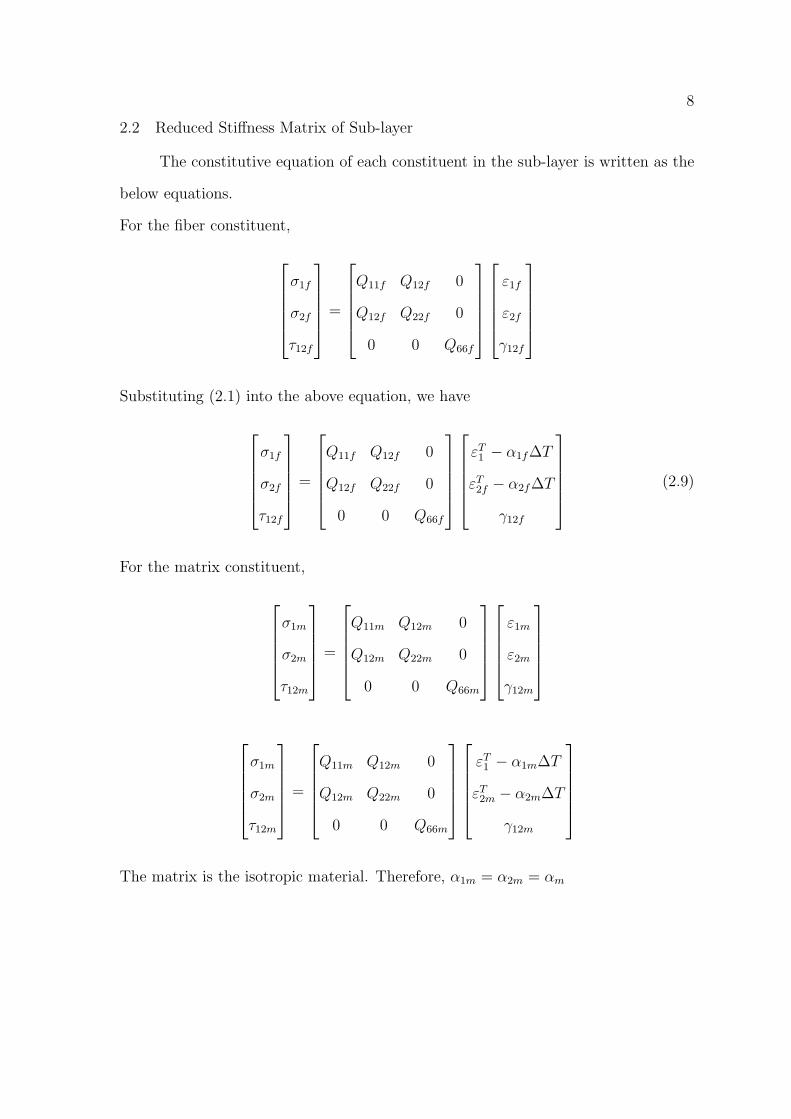
2.2 Reduced Stiffness Matrix of Sub-layer

The constitutive equation of each constituent in the sub-layer is written as the

below equations.

For the fiber constituent,

σ1f

σ2f

τ12f

=

Q11f Q12f 0

Q12f Q22f 0

0 0 Q66f

ε1f

ε2f

γ12f

Substituting (2.1) into the above equation, we have

σ1f

σ2f

τ12f

=

Q11f Q12f 0

Q12f Q22f 0

0 0 Q66f

εT1 − α1f∆T

εT2f − α2f∆T

γ12f

(2.9)

For the matrix constituent,

σ1m

σ2m

τ12m

=

Q11m Q12m 0

Q12m Q22m 0

0 0 Q66m

ε1m

ε2m

γ12m

σ1m

σ2m

τ12m

=

Q11m Q12m 0

Q12m Q22m 0

0 0 Q66m

εT1 − α1m∆T

εT2m − α2m∆T

γ12m

The matrix is the isotropic material. Therefore, α1m = α2m = αm

9σ1m

σ2m

τ12m

=

Q11m Q12m 0

Q12m Q22m 0

0 0 Q66m

εT1 − αm∆T

εT2m − αm∆T

γ12m

(2.10)

For the whole unit cell layer,

σ1

σ2

τ12

=

Q11 Q12 0

Q12 Q22 0

0 0 Q66

ε1

ε2

γ12

σ1

σ2

τ12

=

Q11 Q12 0

Q12 Q22 0

0 0 Q66

εT1 − α1∆T

εT2 − α2∆T

γ12

(2.11)

Substituting both Equations (2.9) and (2.10) into Equations (2.2), (2.3) and

(2.4), we obtain

σ1 = (Q11fVf +Q11mVm)εT1 +Q12fVfε

T2f +Q12mVmε

T2m

− [(Q11fα1f +Q12fα2f )Vf + (Q11mαm +Q12mαm)Vm]∆T

(2.12)

With σ2 = σ2f , we have

σ2 = Q12fεT1 +Q22fε

T2f − (Q12fα1f +Q22fα2f )∆T (2.13)

Since σ2 = σ2m, we have

σ2 = Q12mεT1 +Q22mε

T2m − (Q12mαm +Q22mαm)∆T (2.14)

10

τ12f = Q66fγ12f (2.15)

τ12m = Q66mγ12m (2.16)

Where εT2f and εT2m are still unknown and they will be expressed in the term of

εT1 , εT2 and ∆T .

From the constitutive equation of each constituent in the sub-layer, the following

relationships can be obtained.

σ2f = Q12fεT1 +Q22fε

T2f − (Q12fα1f +Q22fα2f )∆T (2.17)

σ2m = Q12mεT1 +Q22mε

T2m − (Q12mαm +Q22mαm)∆T (2.18)

Since σ2f = σ2m, we can rewrite εT2f and εT2m as shown below

εT2m =1

Q22m

[(Q12f−Q12m)εT1 +Q22fε

T2f+(Q12mαm+Q22mαm−Q12fα1f−Q22fα2f )∆T ]

(2.19)

εT2f =1

Q22f

[(Q12m−Q12f )εT1 +Q22mε

T2m+(Q12fα1f+Q22fα2f−Q12mαm−Q22mαm)∆T ]

(2.20)

Substituting Equations (2.19) and (2.20) into Equation (2.5) respectively, then

εT2f and εT2m can be obtain in terms of εT1 , εT2 and ∆T as expressed:

εT2f is firstly considered.

11

εT2 = εT2fVf+Vm

Q22m

[(Q12f−Q12m)εT1+Q22fε

T2f+(Q12mαm+Q22mαm−Q12fα1f−Q22fα2f )∆T ]

εT2 =Q22mVf +Q22fVm

Q22m

εT2f +Vm(Q12f −Q12m)

Q22m

εT1

+Vm

Q22m

(Q12mαm +Q22mαm −Q12fα1f −Q22fα2f )∆T

εT2f =Q22m

Q22mVf +Q22fVm

εT2 +Vm(Q12m −Q12f )

Q22mVf +Q22fVm

εT1

+Vm(Q12fα1f +Q22fα2f −Q12mαm −Q22mαm)

Q22mVf +Q22fVm

∆T

(2.21)

Similarly, εT2m can be obtained from Equation (2.5) as shown below.

εT2 =Q22mVf +Q22fVm

Q22f

εT2m +Vf (Q12m −Q12f )

Q22f

εT1

+Vf

Q22f

(Q12fα1f +Q22fα2f −Q12mαm −Q22mαm)∆T

εT2m =Q22f

Q22mVf +Q22fVm

εT2 +Vf (Q12f −Q12m)

Q22mVf +Q22fVm

εT1

+Vf (Q12mαm +Q22mαm −Q12fα1f −Q22fα2f )

Q22mVf +Q22fVm

∆T

(2.22)

For the shear term, from Equations (2.3) and (2.15) the following relationship

is obtained.

γ12m =Q66fγ12fQ66m

Substituting above equation in Equation (2.6), then γ12f can be obtained in

terms of γ12.

12

γ12 = γ12fVf + γ12mVm

γ12 = γ12fVf +Q66fγ12fQ66m

Vm

γ12 = γ12f (Vf +Q66f

Q66m

Vm)

γ12f =Q66m

Q66mVf +Q66fVm

γ12 (2.23)

Combining Equations (2.18), (2.19) and (2.20) into Equations (2.11), (2.12) and

(2.13), we can obtain the reduced stiffness of the unit cell layer in terms of the reduced

stiffness of each constituent and its volume fraction. The constitutive equation of the

unit cell layer can be written as Equation (2.11).

σ1

σ2

τ12

=

Q11 Q12 0

Q12 Q22 0

0 0 Q66

εT1 − α1∆T

εT2 − α2∆T

γT12

The reduced stiffness matrix of each sub-layer in terms of the stiffness of each

constituent and its volume fraction are expressed as following.

The stress in 1-direction is considered first,

σ1 = Q11(εT1 − α1∆T ) +Q12(ε

T2 − α2∆T )

σ1 = Q11εT1 +Q12ε

T2 − (Q11α1 +Q12α2)∆T (2.24)

13

Then consider (2.12),

σ1 = (Q11fVf +Q11mVm)εT1 +Q12fVfε

T2f +Q12mVmε

T2m

− [(Q11fα1f +Q12fα2f )Vf + (Q11mαm +Q12mαm)Vm]∆T

Substitute εT2f and εT2m into Equation (2.12) and rearrange it in term of εT1 , εT2 and

∆T .

σ1 = [Q11fVf +Q11mVm +Q12fVfVm(Q12m −Q12f )

Q22mVf +Q22fVm

+Q12mVmVf (Q12f −Q12m)

Q22mVf +Q22fVm

]εT1

+ [Q12fQ22mVf

Q22mVf +Q22fVm

+Q12mQ22fVm

Q22mVf +Q22fVm

]εT2

+ [VfVm(Q12f −Q12m)(Q12fα1f +Q22fα2f −Q12mαm −Q22mαm)

Q22mVf +Q22fVm

− {(Q11fα1f +Q12fα2f )Vf + (Q11mαm +Q12mαm)Vm}]∆T

(2.25)

Equating (2.24) and (2.25), Q11 and Q12can be obtained as.

Q11 = Q11fVf +Q11mVm +Q12fVfVm(Q12m −Q12f )

Q22mVf +Q22fVm

+Q12mVmVf (Q12f −Q12m)

Q22mVf +Q22fVm

Or

Q11 = (Q11f −Q11m)Vf +Q11m −(Vf − V 2

f )(Q12m −Q12f )2

(Q22m −Q22f )Vf +Q22f

(2.26)

14

Q12 =Q12fQ22mVf

Q22mVf +Q22fVm

+Q12mQ22fVm

Q22mVf +Q22fVm

Or

Q12 =(Q12fQ22m −Q12mQ22f )Vf +Q12mQ22f

(Q22m −Q22f )Vf +Q22f

(2.27)

The thermal related terms can be obtained as

−(Q11α1 +Q12α2) =VfVm(Q12f −Q12m)(Q12fα1f +Q22fα2f −Q12mαm −Q22mαm)

Q22mVf +Q22fVm

− [(Q11fα1f +Q12fα2f )Vf + (Q11mαm +Q12mαm)Vm]

Let Vm = 1− Vf and eliminate minus sign in both sides,

Q11α1 +Q12α2 =(Vf − V 2

f )(Q12m −Q12f )(Q12fα1f +Q22fα2f −Q12mαm −Q22mαm)

(Q22m −Q22f )Vf +Q22f

+ (Q11fα1f +Q12fα2f −Q11mαm −Q12mαm)Vf + (Q11mαm +Q12mαm)

(2.28)

Let assume the above equation into this form in order to simplify,

Q11α1 +Q12α2 = C1 (2.29)

Similarly, the stress in 2-direction can be obtained as

σ2 = Q12εT1 +Q22ε

T2 − (Q12α1 +Q22α2)∆T (2.30)

From Equation (2.13),

15

σ2 = Q12fεT1 +Q22fε

T2f − (Q12fα1f +Q22fα2f )∆T

Substitute εT2f into Equation (2.13) and rearrange it into the terms of εT1 , εT2 and

∆T .

σ2 =Q12fQ22mVf +Q12mQ22fVm

Q22mVf +Q22fVm

εT1 +Q22fQ22m

Q22mVf +Q22fVm

εT2

+ [Q22fVm(Q12fα1f +Q22fα2f −Q12mαm −Q22mαm)

Q22mVf +Q22fVm

− (Q12fα1f +Q22fα2f )]∆T

(2.31)

Equating (2.30) and (2.31), Q22 can be obtained as

Q22 =Q22fQ22m

(Q22m −Q22f )Vf +Q22f

(2.32)

The thermal related terms are obtained as

−(Q12α1 +Q22α2) =Q22fVm(Q12fα1f +Q22fα2f −Q12mαm −Q22mαm)

Q22mVf +Q22fVm

− (Q12fα1f +Q22fα2f )

Let Vm = 1− Vf and eliminate minus sign in both sides,

Q12α1 +Q22α2 =Q22f (Q12fα1f +Q22fα2f −Q12mαm −Q22mαm)(Vf − 1)

(Q22m −Q22f )Vf +Q22f

+Q12fα1f +Q22fα2f

(2.33)

Let assume the above equation into this form in order to simplify,

Q12α1 +Q22α2 = C2 (2.34)

16

The coefficient of thermal expansion, α1 and α2, are obtained by solving Equation

(2.29) and (2.34).

α1 =Q22C1 −Q12C2

Q11Q22 −Q212

(2.35)

α2 =Q11C2 −Q12C1

Q11Q22 −Q212

(2.36)

The corresponding shear stress is given as

τ12 = Q66γ12 (2.37)

Using (2.15),

τ12f = Q66fγ12f

Substituting γ12f from (2.23), the τ12f can be obtained in term of γ12.

τ12f =Q66fQ66m

Q66mVf +Q66fVm

γ12 (2.38)

Equating (2.37) and (2.38), Q66 can be obtained as

Q66 =Q66fQ66m

(Q66m −Q66f )Vf +Q66f

(2.39)

The reduced stiffness matrix, [Q], of the fiber and matrix constituents is given

as

17

Q11f =E1f

1− v12fv21f(2.40)

Q12f =E1fv21f

1− v12fv21f(2.41)

Q22f =E2f

1− v12fv21f(2.42)

Q66f = G12f (2.43)

Q11m =Em

1− v2m(2.44)

Q12m =Emvm1− v2m

(2.45)

Q22m =Em

1− v2m(2.46)

Q66m = G12m (2.47)

2.3 Laminate Stiffness and Thermal Resultant Matrices

The laminate stiffness matrices, [A], [B], and [D] can be obtained by integrating

the reduced stiffness matrix, [Q], through the thickness of the unit cell layer. For the

integration, the component of [Q] from Equation (2.26), (2.27), (2.32) and (2.34) are

referred. The expressions of the components of these matrices are shown as below.

A11 =

∫ h/2

−h/2

Q11 dz =

∫ −a

−h/2

Q11 dz +

∫ a

−a

Q11 dz +

∫ h/2

a

Q11 dz

18

A11 = Q11mh+ (Q11f −Q11m)I1 − (Q12m −Q12f )2(I5 − I6) (2.48)

A12 =

∫ h/2

−h/2

Q12 dz = Q12m(h−2a)+(Q12fQ22m−Q12mQ22f )I5+Q12mQ22fI4 (2.49)

A22 =

∫ h/2

−h/2

Q22 dz = Q22m(h− 2a) +Q22mQ22fI4 (2.50)

A66 =

∫ h/2

−h/2

Q66 dz = Q66m(h− 2a) +Q66mQ66fI4∗ (2.51)

As expected,

A16 =

∫ h/2

−h/2

Q16 dz = 0 (2.52)

A26 =

∫ h/2

−h/2

Q26 dz = 0 (2.53)

B11 =

∫ h/2

−h/2

Q11z dz = 0 (2.54)

B12 =

∫ h/2

−h/2

Q12z dz = 0 (2.55)

B22 =

∫ h/2

−h/2

Q22z dz = 0 (2.56)

B66 =

∫ h/2

−h/2

Q66z dz = 0 (2.57)

B16 =

∫ h/2

−h/2

Q16z dz = 0 (2.58)

19

B26 =

∫ h/2

−h/2

Q26z dz = 0 (2.59)

D11 =

∫ h/2

−h/2

Q11z2 dz =

∫ −a

−h/2

Q11z2 dz +

∫ a

−a

Q11z2 dz +

∫ h/2

a

Q11z2 dz

D11 = Q11mh3

12+ (Q11f −Q11m)I13 − (Q12m −Q12f )

2(I15 − I16) (2.60)

D12 =

∫ h/2

−h/2

Q12z2 dz = Q12m(

h3

12− 2a3

3) + (Q12fQ22m −Q12mQ22f )I15 +Q12mQ22fI14

(2.61)

D22 =

∫ h/2

−h/2

Q22z2 dz = Q22m(

h3

12− 2a3

3) +Q22mQ22fI14 (2.62)

D66 =

∫ h/2

−h/2

Q66z2 dz = Q66m(

h3

12− 2a3

3) +Q66mQ66fI14

∗ (2.63)

D16 =

∫ h/2

−h/2

Q16z2 dz = 0 (2.64)

D26 =

∫ h/2

−h/2

Q26z2 dz = 0 (2.65)

Where the list of I parameters are provided in Appendix A.

The thermal resultant and moment matrices, [N t] and [M t], can be obtained

by integrating the constitutive equation of the unit cell layer. The procedure and

expression of the thermal resultant matrices are shown as below.

The constitutes equation of the unit cell layer,

20

[σ]1,2 = [Q]1,2[εT ]1,2 − [Q]1,2[α]1,2∆T

From [εT ]1,2 = [ε0]1,2 + z[k]1,2

[σ]1,2 = [Q]1,2[ε0]1,2 + z[Q]1,2[k]1,2 − [Q]1,2[α]1,2∆T (2.66)

Integration of the stresses from Equation (2.66) across the all thickness in lam-

inate gives the force resultants:

[N ]1,2 =

∫ h/2

−h/2

[σ]1,2 dz

[N ]1,2 =

∫ h/2

−h/2

{[Q]1,2[ε

0]1,2 + z[Q]1,2[k]1,2 − [Q]1,2[α]1,2∆T}dz

[N ]1,2 = [A]1,2[ε0]1,2 + [B]1,2[k]1,2 − [N t]1,2 (2.67)

Therefore, the themal resultant matrix is obtained.

[N t]1,2 =

∫ h/2

−h/2

[Q]1,2[α]1,2∆T dz

or, in view,

N t

1

N t2

N t12

=

∫ h/2

−h/2

Q11 Q12 0

Q12 Q22 0

0 0 Q66

α1∆T

α2∆T

0

dz (2.68)

21

First, the thermal resultant in 1-direction is considered.

N t1 =

∫ h/2

−h/2

{Q11α1∆T +Q12α2∆T} dz

N t1 = ∆T

∫ h/2

−h/2

{Q11

Q22C1 −Q12C2

Q11Q22 −Q212

+Q12Q11C2 −Q12C1

Q11Q22 −Q212

}dz

N t1 = ∆T

∫ h/2

−h/2

{Q11Q22C1 −Q11Q12C2 +Q11Q12C2 −Q2

12C1

Q11Q22 −Q212

}dz

N t1 = ∆T

∫ h/2

−h/2

{Q11Q22 −Q2

12

Q11Q22 −Q212

C1

}dz

Where, C1 is from Equation (2.28) and (2.29).

C1 =(Vf − V 2

f )(Q12m −Q12f )(Q12fα1f +Q22fα2f −Q12mαm −Q22mαm)

(Q22m −Q22f )Vf +Q22f

+ (Q11fα1f +Q12fα2f −Q11mαm −Q12mαm)Vf + (Q11mαm +Q12mαm)

Therefore,

N t1 = ∆T

∫ h/2

−h/2

C1 dz = ∆T

{∫ −a

−h/2

C1 dz +

∫ a

−a

C1 dz +

∫ h/2

a

C1 dz

}

N t1 = ∆T [(Q11mαm +Q12mαm)h+ (Q11fα1f +Q12fα2f −Q11mαm −Q12mαm)I1

+ (Q12m −Q12f )(Q12fα1f +Q22fα2f −Q12mαm −Q22mαm)(I5 − I6)]

(2.69)

22

Then, the thermal resultant in 2-direction is considered.

N t2 =

∫ h/2

−h/2

{Q12α1∆T +Q22α2∆T} dz

N t2 = ∆T

∫ h/2

−h/2

{Q12

Q22C1 −Q12C2

Q11Q22 −Q212

+Q22Q11C2 −Q12C1

Q11Q22 −Q212

}dz

N t2 = ∆T

∫ h/2

−h/2

{Q12Q22C1 −Q2

12C2 +Q11Q22C2 −Q12Q22C1

Q11Q22 −Q212

}dz

N t2 = ∆T

∫ h/2

−h/2

{Q11Q22 −Q2

12

Q11Q22 −Q212

C2

}dz

Where, C2 is from (2.33) and (2.34).

C2 =Q22f (Q12fα1f +Q22fα2f −Q12mαm −Q22mαm)(Vf − 1)

(Q22m −Q22f )Vf +Q22f

+Q12fα1f +Q22fα2f

Therefore,

N t2 = ∆T

∫ h/2

−h/2

C2 dz = ∆T

{∫ −a

−h/2

C2 dz +

∫ a

−a

C2 dz +

∫ h/2

a

C2 dz

}

N t2 = ∆T [(Q12fα1f +Q22fα2f )h− (Q12fα1f +Q22fα2f −Q12mαm −Q22mαm)(h− 2a)

+Q22f (Q12fα1f +Q22fα2f −Q12mαm −Q22mαm)(I5 − I4)]

(2.70)

23

Integration of the stresses and height from Equation (2.66) across the all thick-

ness in laminate gives the thermal moment:

[M ]1,2 =

∫ h/2

−h/2

z[σ]1,2 dz

Therefore,

[M ]1,2 =

∫ h/2

−h/2

{z[Q]1,2[ε

0]1,2 + z2[Q]1,2[k]1,2 − z[Q]1,2[α]1,2∆T}dz

[M ]1,2 = [B]1,2[ε0]1,2 + [D]1,2[k]1,2 − [M t]1,2 (2.71)

Therefore, the themal moment matrix is obtained.

[M t]1,2 =

∫ h/2

−h/2

z[Q]1,2[α]1,2∆T dz

or, in view,

M t

1

M t2

M t12

=

∫ h/2

−h/2

z

Q11 Q12 0

Q12 Q22 0

0 0 Q66

α1∆T

α2∆T

0

dz (2.72)

With the same way that is used to get the thermal resultant matrix, the thermal

moment matrix is obtained.

M t1 = ∆T

∫ h/2

−h/2

zC1 dz = 0 (2.73)

24

M t2 = ∆T

∫ h/2

−h/2

zC2 dz = 0 (2.74)

As expected, [M t] = 0

2.4 Methods of Obtaining the Effective Properties

The laminate compliances matrices, [a], [b], [b]T and [d], can be obtained from

the inversion of the laminate stiffness matrices, [A], [B], and [D], as shown below.

a b

bT d

=

A B

B D

−1

(2.75)

The effective moduli of the laminates can be obtained by the extensional lami-

nate compliance matrix, [a], and the entire unit cell thichness, t, as shown below.

E1 =1

a11t(2.76)

E2 =1

a22t(2.77)

For a symmetric and banlanced laminate, the coupling stiffness matrix, [B],

will be zero that make the coupling compliance matrices, [b] and [b]T go to zero, .

With this condition, the effective moduli of the laminate can be directly get from the

laminate stiffness matrix, [A], as listed below.

E1 = (A11 −A2

12

A22

)1

t(2.78)

E2 = (A22 −A2

12

A11

)1

t(2.79)

25

To get the coefficients of thermal expansion, α1 and α2, the mid plane strain,

ε1 and ε2, need to be obtained by assume no external force and moment in Equation

(2.67) and (2.71).

Considering (2.67) without mechanical force, we have

[N t]1,2 = [A]1,2[ε0]1,2 + [B]1,2[k]1,2 (2.80)

From [B] = 0,

[N t]1,2 = [A]1,2[ε0]1,2

Inverse the above equation.

[ε0]1,2 = [a]1,2[Nt]1,2 (2.81)

ε01

ε02

γ012

=

a11 a12 0

a12 a22 0

0 0 a66

N t

1

N t2

0

(2.82)

Therefore,

ε01 = a11Nt1 + a12N

t2 (2.83)

ε02 = a12Nt1 + a22N

t2 (2.84)

γ012 = 0 (2.85)

26

Then, consider Equation (2.70) without extenal moment.

0 = [B]1,2[ε0]1,2 + [D]1,2[k]1,2 − [M t]1,2

[M t]1,2 = [B]1,2[ε0]1,2 + [D]1,2[k]1,2 (2.86)

From [M t]1,2 = 0 and [B]1,2 = 0,

[D]1,2[k]1,2 = 0

[k]1,2 = 0 (2.87)

From Equation (2.82) and (2.83), the coefficient of thermal expansion can be

get in the below equation.

First, consider the longitudinal coefficient of thermal expansion.

α1∆T = ε01 (2.88)

Therefore,

α1 =ε01∆T

(2.89)

Do the same approach for the transverse coefficient of thermal expansion. Thus,

α2 =ε02∆T

(2.90)

27

2.5 Stresses Components due to Thermal Expansion

With this present solution, the stress components of the fiber and matrix can

also be estimated by any given z position. From Equation (2.8), the fiber volume

fraction in each layer can be obtained with the z position.

Vf =

0 z ∈ [−h2,−a] ∪ [a, h

2]

wi

W= 2b

W

√1− z2

a2z ∈ [−a, a]

The stress, σ1f and σ1m of a given sublayer can be obtained from Equations

(2.9) and (2.10).

σ1f = Q11fεT1 +Q12fε

T2f − (Q11fα1f +Q12fα2f )∆T

σ1m = Q11mεT1 +Q12mε

T2m − (Q11mαm +Q12mαm)∆T

Where εT1 , εT2f and εT2m are given in Equations (2.21) and (2.22).

σ2f and σ2m of the given sublayer is shown in Equations (2.17) and (2.18). It

should be noted that γ12 ≡ 0 resulting in τ12 = τ12f = τ12m = 0.

2.6 Rule-of-Mixture and Schapery’s Methods

Rule of Mixture is a conventional method to estimate the properties of compos-

ite material, based on the properties and volume fraction of each constituent. The

effective moduli and the coefficients of thermal expansion from the Rule of Mixture

are expressed as below equations.

For the longitudinal modulus,

28

E1 = E1fVf + EmVm (2.91)

For the transverse modulus,

1

E2

=Vf

E2f

+Vm

Em

(2.92)

For Poissons ratio,

v12 = v12fVf + v12mVm (2.93)

For the shear modulus,

1

G12

=Vf

G12f

+Vm

Gm

(2.94)

Unlike the effective moduli, CTE’s does not follow the ROM.

The coefficient of thermal expansion in the longitudinal direction (along the

fiber) is given as [12],

α1 =E1fα1fVf + E1mαmVm

E1fVf + E1mVm

(2.95)

The coefficient of thermal expansion in the transverse direction (perpendicular

to the fiber) for isotropic and orthotropic is given as [3],

For the isotropic fiber,

α2 = αfVf (1 + vf ) + αmVm(1 + vm)− v12α1 (2.96)

29

For the orthotropic fiber,

α2 = α2fVf (1 + v12fα1f

α2f

) + αmVm(1 + vm)− v12α1 (2.97)

CHAPTER 3

FINITE ELEMENT ANALYSIS

The finite element model of a unit cell of composite lamina is created to calculate

the effective moduli and coefficients of thermal expansion. A three-dimensional finite

element model is developed in this chapter using ANSYS 11.0 program. The ANSYS

codes are listed in Appendix B. In order to verify the model, the isotropic material

properties are first applied in each model before applying to composite material. The

difference of results in the calculated case and materials properties is less than 0.1%.

3.1 Finite Element Model for Longitudinal Load

3.1.1 Geometric Description

Both circular and elliptical configurations cross-sections of fiber are chosen for

study. Figure 3.1 and 3.2 show the description of the unit cell geometries used in this

study.

In fiber volume fraction study, the fiber volume fraction, Vf , is independent

variable. Due to the square array model, the width and height, W and h, are fixed

at 0.005 inch. The radius, r, that is the dependent variable can be calculated from

the fiber volume fraction and the width of the unit cell. For elliptical cross-section

of fiber, Vf and a (the semi-major axis) are given, then b (the semi-minor axis) is

determined. The length of model of unit cell is 10 times of the width.

30

31

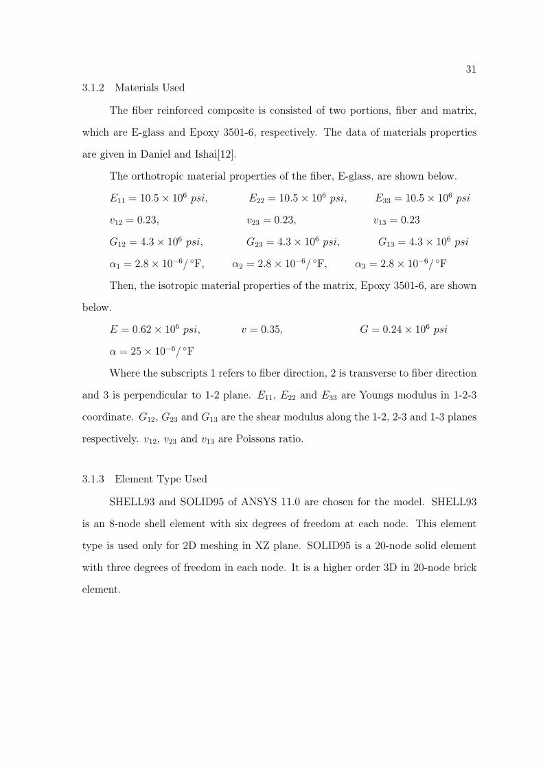
3.1.2 Materials Used

The fiber reinforced composite is consisted of two portions, fiber and matrix,

which are E-glass and Epoxy 3501-6, respectively. The data of materials properties

are given in Daniel and Ishai[12].

The orthotropic material properties of the fiber, E-glass, are shown below.

E11 = 10.5× 106 psi, E22 = 10.5× 106 psi, E33 = 10.5× 106 psi

v12 = 0.23, v23 = 0.23, v13 = 0.23

G12 = 4.3× 106 psi, G23 = 4.3× 106 psi, G13 = 4.3× 106 psi

α1 = 2.8× 10−6/ ◦F, α2 = 2.8× 10−6/ ◦F, α3 = 2.8× 10−6/ ◦F

Then, the isotropic material properties of the matrix, Epoxy 3501-6, are shown

below.

E = 0.62× 106 psi, v = 0.35, G = 0.24× 106 psi

α = 25× 10−6/ ◦F

Where the subscripts 1 refers to fiber direction, 2 is transverse to fiber direction

and 3 is perpendicular to 1-2 plane. E11, E22 and E33 are Youngs modulus in 1-2-3

coordinate. G12, G23 and G13 are the shear modulus along the 1-2, 2-3 and 1-3 planes

respectively. v12, v23 and v13 are Poissons ratio.

3.1.3 Element Type Used

SHELL93 and SOLID95 of ANSYS 11.0 are chosen for the model. SHELL93

is an 8-node shell element with six degrees of freedom at each node. This element

type is used only for 2D meshing in XZ plane. SOLID95 is a 20-node solid element

with three degrees of freedom in each node. It is a higher order 3D in 20-node brick

element.

32

3.1.4 Modeling and Mesh Generation

The modeling and mesh generation is done using ANSYS 11.0 preprocessor tool.

The procedure used to develop a square array model is described below.

1. Define SHELL93 as element type 1 and SOLID95 as element type 2.

2. Define the material properties of E-glass as material model 1 and the material

properties of Epoxy 3501-6 as material model 2.

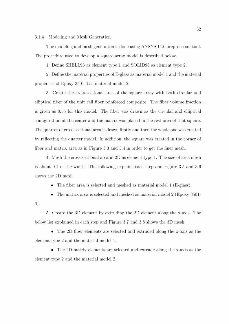
3. Create the cross-sectional area of the square array with both circular and

elliptical fiber of the unit cell fiber reinforced composite. The fiber volume fraction

is given as 0.55 for this model. The fiber was drawn as the circular and elliptical

configuration at the center and the matrix was placed in the rest area of that square.

The quarter of cross sectional area is drawn firstly and then the whole one was created

by reflecting the quarter model. In addition, the square was created in the corner of

fiber and matrix area as in Figure 3.3 and 3.4 in order to get the finer mesh.

4. Mesh the cross sectional area in 2D as element type 1. The size of area mesh

is about 0.1 of the width. The following explains each step and Figure 3.5 and 3.6

shows the 2D mesh.

• The fiber area is selected and meshed as material model 1 (E-glass).

• The matrix area is selected and meshed as material model 2 (Epoxy 3501-

6).

5. Create the 3D element by extruding the 2D element along the x-axis. The

below list explained in each step and Figure 3.7 and 3.8 shows the 3D mesh.

• The 2D fiber elements are selected and extruded along the x-axis as the

element type 2 and the material model 1.

• The 2D matrix elements are selected and extrude along the x-axis as the

element type 2 and the material model 2.

33

• The all 2D elements are deleted and the all 3D elements are merged all

nodes.

3.1.5 Boundary and Loading Conditions

To determine the mechanical properties in this model, a mechanical load is

applied. The yz-plane at the edge of the model is coupled to ensure the uniform

deformation in x-direction because of the perfect bonding assumption. The corre-

sponding boundary conditions are listed below.

1. All the nodes at x=0 are constrained along x-axis (loading axis) i.e. Ux=0.

2. All the nodes at y=0 are constrained along y-axis (loading axis) i.e. Uy=0.

3. All the nodes at z=0 are constrained along z-axis (loading axis) i.e. Uz=0.

4. All the nodes at end of the unit cell (x=L) are coupled along x-axis to get

the uniform deformation in x-direction.

5.All the nodes at top and bottom of the unit cell in y-direction (y=W/2,-W/2)

are coupled along y-axis to get the uniform deformation in y-direction.

6.All the nodes at top and bottom of the unit cell in z-direction (z=W/2,-W/2)

are coupled along z-axis to get the uniform deformation in z-direction.

7. Apply the longitudinal load, Fx = 1, at x = L, y = 0 and z = 0.

3.2 Finite Element Model for Thermal Load

Due to the same configuration, material and element type, this model can use

all steps in longitudinal load model except the boundary condition.

For thermal load application only, the boundary conditions of the model is

different from the previous case.

34


The boundary conditions of this model do not have the mechanical load because

it was created to study the coefficient of thermal expansion. Hence, only uniform

temperature was applied in all nodes. The list below shows all boundary conditions

of this model.

1. All the nodes at x=0 are constrained along x-axis (loading axis) i.e. Ux=0.



4. All the nodes at end of the unit cell (x=L) are coupled along x-axis to get

the uniform deformation in x-direction.

5.All the nodes at top and bottom of the unit cell in y-direction (y=W/2,-W/2)

are coupled along y-axis to get the uniform deformation in y-direction.

6.All the nodes at top and bottom of the unit cell in z-direction (z=W/2,-W/2)


7. All nodes are added the temperature reference and the uniform temperature

to get ∆T .

3.3 Finite Element Model for Transverse Load

3.3.1 Geometric Description

The model used in this case is not different from the previous case. To reduce

the size of model, a shorter length of the model is used. The length in this model

is only 0.1 of the width. Therefore, only the 3D mesh of this models are shown in

Figure 3.9 and 3.10.

35


Boundary conditions of this model are given below:

1. All the nodes at x=L/2 are constrained along x-axis (loading axis) i.e. Ux=0.



4. All the nodes at end of the unit cell (y=W/2) are coupled along x-axis to

get the uniform deformation in x-direction.

5.All the nodes at top and bottom of the unit cell in x-direction (x=0,L) are

coupled along y-axis to get the uniform deformation in y-direction.

6.All the nodes at top and bottom of the unit cell in z-direction (z=W/2,-w/2)


7. Apply the transverse load, Fy = 1, at x = 0, y = W/2 and z = 0.

3.4 Method of Obtaining the Effective Properties

The effective moduli, E1 and E2, and coefficients of thermal expansion, α1 and

α2, can not be directly obtained from the finite element output. These properties can

be calculated as described below.

For the longitudinal and transverse load models,

E1 =Px

Axεx(3.1)

E2 =Py

Ayεy(3.2)

Where εx is the strain of the model in x-direction at x = L and εy is the strain

of this model in y-direction at y = W/2.

36

εx is directly obtained in finite element output like in Figure 3.11 and 3.12.

Unlikely, εy has to be calculate from the deformation at y = W/2 over W/2 which is

shown in Figure 3.13 and 3.14. Px, Py, Ax and Ay are the applied force and the areas

of the model in the x- and y-directions (or yz- and xz-plane), respectively.

For the thermal load model,

α1 =εTx∆T

(3.3)

α2 =εTy∆T

(3.4)

Where εTx is the total strain of the model in x-direction at x = L and εTy is the

total strain of this model in y-direction at y = W/2 or y = −W/2.

εTx is directily obtained in finite element output as in Figure 3.11 and 3.12.

Unlikely, εTy has to be calculate from the deformation at y = W/2 over W/2 which is

also shown in Figure 3.13 and 3.14. ∆T is the difference between the reference and

applied temperature which are applied in the model.

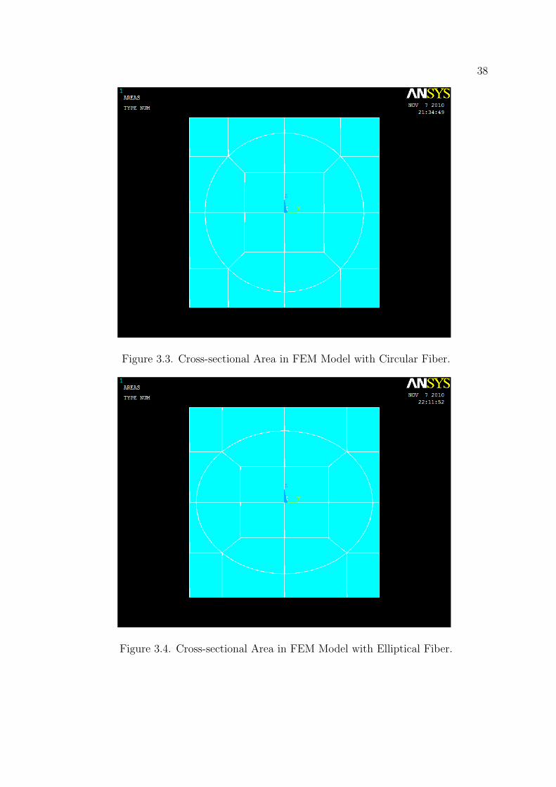
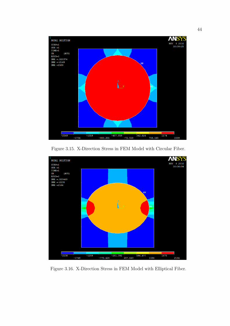
Moreover, the stresses components in x-direction due to the temperature effect

are also directly obtained from FEM result. Figure 3.15 and 3.16 show the stress

contour in FEM model. However, the stresses components can be obtained in the

specific nodes.

With the symmetry model, the quarter model can be determined as the whole

model. Therefore, the quarter FEM model is used to analyze in order to reduce the

time consuming.

37

Figure 3.1. Unit Cell with Circular Fiber.

Figure 3.2. Unit Cell with Elliptical Fiber.

38

Figure 3.3. Cross-sectional Area in FEM Model with Circular Fiber.

Figure 3.4. Cross-sectional Area in FEM Model with Elliptical Fiber.

39

Figure 3.5. 2D-Mesh in FEM Model with Circular Fiber.

Figure 3.6. 2D-Mesh in FEM Model with Elliptical Fiber.

40

Figure 3.7. 3D-Mesh in FEM Model with Circular Fiber.

Figure 3.8. 3D-Mesh in FEM Model with Elliptical Fiber.

41

Figure 3.9. 3D-Mesh in Transverse Load Model with Circular Fiber.

Figure 3.10. 3D-Mesh in Transverse Load Model with Elliptical Fiber.

42

Figure 3.11. X-direction Total Strain in FEM Model with Circular Fiber.

Figure 3.12. X-direction Total Strain in FEM Model with Elliptical Fiber.

43

Figure 3.13. Y-Direction Deformation in FEM Model with Circular Fiber.

Figure 3.14. Y-Direction Deformation in FEM Model with Elliptical Fiber.

44

Figure 3.15. X-Direction Stress in FEM Model with Circular Fiber.

Figure 3.16. X-Direction Stress in FEM Model with Elliptical Fiber.

CHAPTER 4

NUMERICAL RESULTS AND DISCUSSIONS

A unit cell that contains a single E-glass fiber surrounded by the Epoxy 3501-6

matrix was used for this study. The material properties of fiber and matrix con-

stituents are already shown in Chapter 3. The properties of y and z direction are

assumed to be the transverse properties in the case of orthogonal fiber. The width

and thickness of the unit cell are selected as 0.005 inch. In the fiber volume fraction

(Vf ) study, the fiber configuration is considered as the circular and then Vf is varied.

On the other hand, Vf is fixed and the major and minor axis (a and b) are varied in

the axial ratio study. The detail of all studies is described in the each section.

4.1 Effects of Fiber Volume Fraction on Effective Properties

In this section, the effects of the fiber volume fraction (Vf ) on the effective

moduli and Coefficients of Thermal Expansion (CTEs) are discussed. With this

specified geometry of the model, Vf can be varied from 0 to 0.78. Figure 4.1 shows

the size of circular fiber that is affected by increasing Vf . In both analytical solution

and Rule of Mixture (ROM), the result can be accurately obtained by increasing 0.01

of Vf . However, the Finite Element Analysis (FEA) has to solve in each case of Vf .

The number of analysis are 78 which is used too much time to proceed. Therefore,

the 0.05 increase of Vf is used to reduce the time consuming.

Figures 4.2, 4.3, 4.4 and 4.5 separately display the variation of the effective

moduli and CTEs with respect to Vf . In these figures, there are three different meth-

ods which are the analytical solution, ROM and FEA in each figure. The comparative

45

46

Figure 4.1. Fiber Size Varies with Fiber Volume Fraction.

data of these figures are also provided in Appendix D. Figures 4.2 and 4.3 show the

comparison of E1 and E2 caculated by three different methods. Figures 4.4 and 4.5

show the same comparison of α1 and α2 as in the previous figures. As indicated in

these figures, E1 and α1 agree very well among these three methods. The calculated

values of E2 and α2 are different among all the methods. However, the present results

of α2 is closer to the finite element results. The difference of both transverse properties

is depended increasingly on the fiber volume fraction. For the transverse properties,

the difference between analytical solution and FEA reach a maximum about 16% at

Vf=0.65. However, the difference between ROM and FEA is a maximum of 50%

and 37% for E2 and α2, respectively. Therefore, the results between the analytical

solution and FEA are closer than the ones between the ROM and FEA. In addition,

there is a significant difference between in the presented and FEA results when the

radius, r, is close to the width in E2 variation because of the bad mesh in FEM.

47

0 0.1 0.2 0.3 0.4 0.5 0.6 0.7 0.80

2

4

6

8

10

12

14

Vf

E1/

Em

Analytical SolutionRule of MixtureFEM

Figure 4.2. Longitudinal Modulus Respect with Fiber Volume Fraction.

0 0.1 0.2 0.3 0.4 0.5 0.6 0.7 0.81

2

3

4

5

6

7

8

Vf

E2/

Em

Analytical SolutionRule of MixtureFEM

Figure 4.3. Transverse Modulus Respect with Fiber Volume Fraction.

48

0 0.1 0.2 0.3 0.4 0.5 0.6 0.7 0.80.1

0.2

0.3

0.4

0.5

0.6

0.7

0.8

0.9

Vf

CT

E1/

CT

Em

Analytical SolutionSchaperyFEM

Figure 4.4. Longitudinal CTE Respect with Fiber Volume Fraction.

0 0.1 0.2 0.3 0.4 0.5 0.6 0.7 0.80.2

0.3

0.4

0.5

0.6

0.7

0.8

0.9

1

1.1

1.2

Vf

CT

E2/

CT

Em

Analytical SolutionSchaperyFEM

Figure 4.5. Transverse CTE Respect with Fiber Volume Fraction.

49

4.2 Effects of Fiber Configuration on the Effective Properties

The effects of fiber configuration on the effective moduli and CTEs are shown

and discussed in this section, respectively. In the axial ratio (a/b) study, Vf is given

as 0.55. Figure 4.6 illustrated the fiber configuration change with respect to the ratio

of a/b. The detail of each approach is shown in Sec. 4.2.1 and 4.2.2.

Figure 4.6. Fiber Shape Varies with Axial Ratio.

4.2.1 Effects of Fiber Configuration in Analytical Solution

The effects of fiber configurations on the stiffness were studied in the previous

analytical solution by Wang and Chan[8]. Similarly, the effects of the fiber configu-

rations on the effective moduli and CTEs are considered in this analytical solution.

The radius, r, is firstly calculated from the fiber volume fraction and the width. The

sizes of a and b are restricted by the width and thickness of the unit cell layer due to

the specified fiber volume fraction. However, a and b can be obtained by assumed a

and then calculate b from each a. For example, the major axis, a, is defined as 0.84

and gradually increased 0.01 until 1.19 in term of r and then the minor axis, b, can

50

be calculated for each value of a. For this example, the ratios of a/b are varying from

0.70 to 1.42.

The variations of the effective moduli and CTEs with respect to the a/b ratios

for the analytical solution are presented in Figure 4.7 and 4.8. In addition, the

comparative data are listed in appendix C. At the circular fiber, the results are

normalized. When the a/b is increased, the fiber portion in z-direction is extended

while the width of area does not change. The ratios of E1 and α1 slightly change in

this results which agree with assumption that the longitudinal properties will not be

significantly affected by the configuration of fiber. This is because the fiber volume

fraction is fixed as the fiber configuration is changed. Unlikely, the E2 is decreased as

the axial ratio is increased. However, the transverse coefficient of thermal expansion,

α2, is increased for the increasing axial ratio. When the a/b is at the minimum

and maximum, the cross sectional area of the unit cell fiber reinforced composite is

more likely to the sanwich laminate. With the b is close to the width, the transverse

properties will be gradually adjusted to be close to the longitudinal ones. ROM

method is created to estimate the transverse properties of the sanwich composite.

Therefore, the transverse properties is close to the ones from the ROM when the a is

close to the width.

4.2.2 Effects of Fiber Configurations in Finite Element Analysis

Like the analytical solution, the finite element model is also designed in variation

of the axial ratio. However, the finite element model is analyzed for each the axial

ratio. Therefore, the numbers of the result in this study for FEA is less than for

the analytical solution for reduce time consuming. The major axis, a, is gradually

increased 0.02 of radius per the model for the finite element analysis. The example of

51

0.7 0.8 0.9 1 1.1 1.2 1.3 1.4 1.50.8

0.9

1

1.1

1.2

1.3

1.4

1.5

1.6

1.7

1.8

Ratio (a/b)

Ei*

/Ei

E1*/E1E2*/E2

Figure 4.7. Moduli Ratio Respect with Axial Ratio in Analytical Solution.

0.7 0.8 0.9 1 1.1 1.2 1.3 1.40.8

0.9

1

1.1

1.2

1.3

1.4

1.5

1.6

Ratio (a/b)

Ei*

/Ei

E1FEM*/E1FEME2FEM*/E2FEM

Figure 4.8. Moduli Ratio Respect with Axial Ratio in FEM.

52

0.7 0.8 0.9 1 1.1 1.2 1.3 1.4 1.50.5

0.6

0.7

0.8

0.9

1

1.1

1.2

1.3

Ratio (a/b)

CT

Ei*

/CT

Ei

CTE1*/CTE1CTE2*/CTE2

Figure 4.9. CTE Ratio Respect with Axial Ratio in Analytical Solution.

0.7 0.8 0.9 1 1.1 1.2 1.3 1.40.5

0.6

0.7

0.8

0.9

1

1.1

1.2

1.3

1.4

Ratio (a/b)

CT

Ei*

/CT

Ei

CTE1FEM*/CTE1FEMCTE2FEM*/CTE2FEM

Figure 4.10. CTE Ratio Respect with Axial Ratio in FEM.

53

0.7 0.8 0.9 1 1.1 1.2 1.3 1.4 1.50.8

0.9

1

1.1

1.2

1.3

1.4

1.5

1.6

1.7

1.8

Ratio (a/b)

Ei*

/Ei

E1*/E1E2*/E2E1FEM*/E1FEME2FEM*/E2FEM

Figure 4.11. Moduli Ratio Respect with Axial Ratio in Both Solutions.

0.7 0.8 0.9 1 1.1 1.2 1.3 1.4 1.50.5

0.6

0.7

0.8

0.9

1

1.1

1.2

1.3

1.4

Ratio (a/b)

CT

Ei*

/CT

Ei

CTE1*/CTE1CTE2*/CTE2CTE1FEM*/CTE1FEMCTE2FEM*/CTE2FEM

Figure 4.12. CTE Ratio Respect with Axial Ratio in Both Solutions.

54

the different model that change the a is already shown in Chapter 3, Figure 3.3 and

3.4.

The variations of the effective modul CTE with respect to the a/b ratios for the

finite element analysis are shown in Figure 4.9 and 4.10. Similar to the variation from

the analytical solution, the ratios of E1 and α1 is close to 1.00 (or 100%) as expect.

For the ratios of E2 and α2 the curve is also similar to the one from analytical solution.

However, the slopes of curves are greater. In addition, the E2 result from FEA shows

an error in the low axial ratio because the minor axis, b, is really close to the width.

Finally, the variations of the same property respect to the a/b from both ana-

lytical solution and FEA is also shown in the same figure for a comparison. Figure

4.11 and 4.12 are shown the variations of the effective moduli, E1 and E2, and the

coefficients of thermal expansion, α1 and α2, respectively.

4.3 Stress Component Due to Thermal Expansion

Typically, the stress components can be evaluated at the specific nodes in FEM

result. The certain position in x-y-z coordinate system of nodes is required to de-

termine the stress components. However, the present method can also estimate the

stress component in the specific z-position.

The stress components of the FEM result and present method in the various

fiber configuration models are showed in Figure 4.13, 4.14 and 4.15. Figure 4.8

and 4.10 present the stress component in the elliptical fiber models while Figure 4.9

presents the result in the circular fiber model. Due to the difference of CTEs in fiber

and matrix, the stress components are in both tension and compression. The fiber

that is the lower CTE component is in tension while the matrix that is the higher

CTE component is in compression.

55

0 0.5 1 1.5 2 2.5

x 10−3

−2500

−2000

−1500

−1000

−500

0

500

1000

1500

2000

Thickness (z)

Str

ess

in x

−di

rect

ion

Fiber in this solutionMatrix in this solutionFiber in FEMMatrix in FEM

Figure 4.13. Stress Components for a/b < 1.

0 0.5 1 1.5 2 2.5

x 10−3

−2500

−2000

−1500

−1000

−500

0

500

1000

1500

2000

Thickness (z)

Str

ess

in x

−di

rect

ion


Figure 4.14. Stress Components for a/b = 1.

56

0 0.5 1 1.5 2 2.5

x 10−3

−2500

−2000

−1500

−1000

−500

0

500

1000

1500

2000

2500

Thickness (z)

Str

ess

in x

−di

rect

ion


Figure 4.15. Stress Components for a/b > 1.

CHAPTER 5

CONCLUSION

A micromechanics model of a unit cell that contains a fiber and matrix was

developed to evaluate the coefficients of thermal expansion (CTE) for fiber reinforced

composite lamina. The model takes the fiber configuration into consideration in

evaluation of the CTEs. Both circular and elliptical cross-sections of the fiber in the

unit cell were considered in this study. The stress components of the fibers and the

matrix in the unit cell under a temperature environment can also be obtained from

the present model. An ANSY finite element model was used to validate the results of

CTEs and the stress components of the fiber and the matrix in the unit cell obtained

from the present method.

Effect of CTEs due to the fiber volume fraction (Vf ) and the fiber configuration

(a/b, semi-major axis to semi-minor axis ratio of elliptical cross-section) are studied.

In Vf study, the results of the longitudinal CTE obtained by the present method

are in excellent agreement with the results from finite element (FEA) and the Rule-

of-Mixture (ROM) methods. However, the present results of the CTE along the

transverse direction show a significant difference from the ROM results but close to

the finite element results. The difference in the results is also dependent on the

fiber volume fraction. In the fiber configuration study, the results of the longitudinal

CTE for both elliptical and circular cross-sections of the fiber indicate no difference.

However, the results in the transverse direction of CTE are significantly different from

each other. It is found that the CTE along the transverse direction increases as the

ratio of a/b increases.

57

58

It should be mentioned that the present model is applicable to the study of

hygroscopic expansion coefficients since the similarity of the hygroscopic and thermal

behavior.

APPENDIX A

THE INTEGRALS USED IN ANALYTICAL SOLUTIONS

59

60

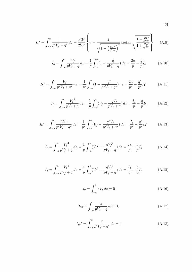
The follow integrals are used for solving the analytical solution. The parameters

p, p∗, q and q∗ are used in the integrals also listed below.

p = Q22m −Q22f (A.1)

q = Q22f (A.2)

p∗ = Q66m −Q66f (A.3)

q∗ = Q66f (A.4)

For Composite Materials

The below list is presented the Ii parameters in composite materials.

I1 =

∫ a

−a

Vf dz =abπ

W(A.5)

I2 =

∫ a

−a

Vf2 dz =

16ab2π

3W 2(A.6)

I3 =

∫ a

−a

Vf3 dz =

3ab3π

W 3(A.7)

I4 =

∫ a

−a

1

pVf + qdz =

aW

2bp

π − 4√1−

(2bpqW

)2arctan

√√√√1− 2bpqW

1 + 2bpqW

(A.8)

61

I4∗ =

∫ a

−a

1

p∗Vf + q∗dz =

aW

2bp∗

π − 4√1−

(2bp∗

q∗W

)2arctan

√√√√1− 2bp∗

q∗W

1 + 2bp∗

q∗W

(A.9)

I5 =

∫ a

−a

Vf

pVf + qdz =

1

p

∫ a

−a

(1− q

pVf + q) dz =

2a

p− q

pI4 (A.10)

I5∗ =

∫ a

−a

Vf

p∗Vf + q∗dz =

1

p∗

∫ a

−a

(1− q∗

p∗Vf + q∗) dz =

2a

p∗− q∗

p∗I4

∗ (A.11)

I6 =

∫ a

−a

Vf2

pVf + qdz =

1

p

∫ a

−a

(Vf −qVf

pVf + q) dz =

I1p− q

pI5 (A.12)

I6∗ =

∫ a

−a

Vf2

p∗Vf + q∗dz =

1

p∗

∫ a

−a

(Vf −q∗Vf

p∗Vf + q∗) dz =

I1p∗

− q∗

p∗I5

∗ (A.13)

I7 =

∫ a

−a

Vf3

pVf + qdz =

1

p

∫ a

−a

(Vf2 − qVf

2

pVf + q) dz =

I2p− q

pI6 (A.14)

I8 =

∫ a

−a

Vf4

pVf + qdz =

1

p

∫ a

−a

(Vf3 − qVf

3

pVf + q) dz =

I3p− q

pI7 (A.15)

I9 =

∫ a

−a

zVf dz = 0 (A.16)

I10 =

∫ a

−a

z

pVf + qdz = 0 (A.17)

I10∗ =

∫ a

−a

z

p∗Vf + q∗dz = 0 (A.18)

62

I11 =

∫ a

−a

zVf

pVf + qdz = 0 (A.19)

I12 =

∫ a

−a

zVf2

pVf + qdz = 0 (A.20)

I13 =

∫ a

−a

z2Vf dz =a3bπ

W(A.21)

I14 =

∫ a

−a

z2

pVf + qdz =

∫ a

−a

a2(1− Vf2)

pVf + qdz = a2(I4 − I6) (A.22)

I14∗ =

∫ a

−a

z2

p∗Vf + q∗dz =

∫ a

−a

a2(1− Vf2)

p∗Vf + q∗dz = a2(I4

∗ − I6∗) (A.23)

I15 =

∫ a

−a

z2Vf

pVf + qdz =

∫ a

−a

a2(1− Vf2)Vf

pVf + qdz = a2(I5 − I7) (A.24)

I16 =

∫ a

−a

z2Vf2

pVf + qdz =

∫ a

−a

a2(1− Vf2)Vf

2

pVf + qdz = a2(I6 − I8) (A.25)

For Isotropic Materials

There is no different between [Q] in the fiber and matrix. Hence, p = 0 and

p∗ = 0. Therefore, some parameters have to be revised.

The below list is presented the revised I parameters for the isotropic materials.

I4 =

∫ a

−a

1

pVf + qdz =

∫ a

−a

1

qdz =

2a

q(A.26)

I4∗ =

∫ a

−a

1

p∗Vf + q∗dz =

∫ a

−a

1

q∗dz =

2a

q∗(A.27)

63

I5 =

∫ a

−a

Vf

pVf + qdz =

∫ a

−a

Vf

qdz =

I1q

(A.28)

I5∗ =

∫ a

−a

Vf

p∗Vf + q∗dz =

∫ a

−a

Vf

q∗dz =

I1q∗

(A.29)

I6 =

∫ a

−a

Vf2

pVf + qdz =

∫ a

−a

Vf2

qdz =

I2q

(A.30)

I6∗ =

∫ a

−a

Vf2

p∗Vf + q∗dz =

∫ a

−a

Vf2

q∗dz =

I2q∗

(A.31)

I7 =

∫ a

−a

Vf3

pVf + qdz =

∫ a

−a

Vf3

qdz =

I3q

(A.32)

I8 =

∫ a

−a

Vf4

pVf + qdz =

∫ a

−a

Vf4

qdz =

256ab4

15qW 4(A.33)

I14 =

∫ a

−a

z2

pVf + qdz =

∫ a

−a

a2(1− Vf2)

qdz =

a2

q(2a− I2) = a2(I4 − I6) (A.34)

I14∗ =

∫ a

−a

z2

p∗Vf + q∗dz =

∫ a

−a

a2(1− Vf2)

q∗dz =

a2

q∗(2a− q∗) = a2(I4

∗ − I6∗) (A.35)

I15 =

∫ a

−a

z2Vf

pVf + qdz =

∫ a

−a

a2(1− Vf2)Vf

qdz =

a2

q(I1 − I3) = a2(I5 − I7) (A.36)

I16 =

∫ a

−a

z2Vf2

pVf + qdz =

∫ a

−a

a2(1− Vf2)Vf

2

qdz =

a2

q(I2 − qI8) = a2(I6 − I8) (A.37)

APPENDIX B

FEM CODES FOR ANSYS 11.0 PROGRAMS

64

65

B.1 ANSYS 11.0 Program for Thermal Expansion Case in Quarter Model

!!!!!!!!!!!!!!!!!!!!!!!!!!!!!!!!!!!!!!!!!!!!!!!!!!!!!!!!!!!!!!!!!!!!!!!!!!!!!!!!!!!!!!!!!!!!!!!!!!!!!!!!!!!!!

/UNITS,BIN

/PREP7

!

! Define Parameter (in)

!

W=5

Pi=3.141592653589793

Vf=0.55

R=(sqrt(Vr/Pi))*W

a=1.00*R

b=Vf*W*W/(Pi*a)

L=10*W

!

! Define Keypoints

!

K,1,0,0,0

K,2,0,R/2,0

K,3,0,R,0

K,4,0,W/2,0

K,5,0,R/2,R/2

K,6,0,R/(sqrt(2)),R/(sqrt(2))

K,7,0,W/2,W/2

K,8,0,0,R/2

K,9,0,0,R

66

K,10,0,0,W/2

K,11,0, b/(sqrt(2)),W/2

K,12,0,W/2, a/(sqrt(2))

!

! Define Lines and Area !

L,1,2

L,2,3

L,5,6

L,1,8

L,8,9

L,2,5

L,5,8

L,4,12

L,12,7

L,7,11

L,11,10

LARC,3,6,1,R

LARC,6,9,1,R

FLST,2,4,4

FITEM,2,2

FITEM,2,12

FITEM,2,6

FITEM,2,3

AL,P51X

FLST,2,4,4

FITEM,2,3

67

FITEM,2,13

FITEM,2,7

FITEM,2,5

AL,P51X

FLST,2,4,4

FITEM,2,6

FITEM,2,1

FITEM,2,4

FITEM,2,7

AL,P51X

FLST,2,3,5,ORDE,2

FITEM,2,1

FITEM,2,-3

ARSCALE,P51X, , ,1,b/R,a/R, ,1,1

L,6,11

L,6,12

L,3,4

L,9,10

FLST,2,4,4

FITEM,2,8

FITEM,2,16

FITEM,2,12

FITEM,2,15

AL,P51X

FLST,2,4,4

FITEM,2,9

68

FITEM,2,15

FITEM,2,10

FITEM,2,14

AL,P51X

FLST,2,4,4

FITEM,2,11

FITEM,2,14

FITEM,2,13

FITEM,2,17

AL,P51X

!

! Element Definition

!

ET,1,SHELL93

ET,2,SOLID95

! material property number 1 E-glass

MP,EX,1,10.5e6

MP,EY,1,10.5e6

MP,EZ,1,10.5e6

MP,PRXY,1,0.23

MP,PRYZ,1,0.23

MP,PRXZ,1,0.23

MP,GXY,1,4.3e6

MP,GYZ,1,4.3e6

MP,GXZ,1,4.3e6

MP,CTEX,1,2.8e-6

69

MP,CTEY,1,2.8e-6

MP,CTEZ,1,2.8e-6

! material property number 2 Epoxy 3501-6

MP,EX,2,0.62e6

MP,EY,2,0.62e6

MP,EZ,2,0.62e6

MP,PRXY,2,0.35

MP,PRYZ,2,0.35

MP,PRXZ,2,0.35

MP,GXY,2,0.24e6

MP,GYZ,2,0.24e6

MP,GXZ,2,0.24e6

MP,CTEX,2,25e-6

MP,CTEY,2,25e-6

MP,CTEZ,2,25e-6

/VIEW,1,1,1,1

/ANG,1

/REP,FAST

APLOT

!

! Meshing 2-D

!

AESIZE,ALL,W/10

FLST,5,3,5,ORDE,2

FITEM,5,1

FITEM,5,-3

70

CM, Y,AREA

ASEL, , , ,P51X

CM, Y1,AREA

CMSEL,S, Y

!*

CMSEL,S, Y1

AATT, 1, , 1, 0,

CMSEL,S, Y

CMDELE, Y

CMDELE, Y1

!*

MSHAPE,0,2D

MSHKEY,1

!*

FLST,5,3,5,ORDE,2

FITEM,5,1

FITEM,5,-3

CM, Y,AREA

ASEL, , , ,P51X

CM, Y1,AREA

CHKMSH,’AREA’

CMSEL,S, Y

!*

AMESH, Y1

!*

CMDELE, Y

71

CMDELE, Y1

CMDELE, Y2

!*

FLST,5,3,5,ORDE,2

FITEM,5,4

FITEM,5,-6

CM, Y,AREA

ASEL, , , ,P51X

CM, Y1,AREA

CMSEL,S, Y

!*

CMSEL,S, Y1

AATT, 2, , 1, 0,

CMSEL,S, Y

CMDELE, Y

CMDELE, Y1

!*

FLST,5,3,5,ORDE,2

FITEM,5,4

FITEM,5,-6

CM, Y,AREA

ASEL, , , ,P51X

CM, Y1,AREA

CHKMSH,’AREA’

CMSEL,S, Y

!*

72

AMESH, Y1

!*

CMDELE, Y

CMDELE, Y1

CMDELE, Y2

!*

/UI,MESH,OFF

!

! 3D Mesh Generation by Extruding

!

TYPE, 2

EXTOPT,ESIZE,80,0,

EXTOPT,ACLEAR,0

!*

EXTOPT,ATTR,0,0,0

MAT,1

REAL, Z4

ESYS,0

!*

FLST,2,3,5,ORDE,2

FITEM,2,1

FITEM,2,-3

VEXT,P51X, , ,L,0,0,,,,

TYPE, 2

EXTOPT,ESIZE,80,0,

EXTOPT,ACLEAR,0

73

!*

EXTOPT,ATTR,0,0,0

MAT,2

REAL, Z4

ESYS,0

!*

FLST,2,3,5,ORDE,2

FITEM,2,4

FITEM,2,-6

VEXT,P51X, , ,L,0,0,,,,

!

!* Deleting 2D Mesh

!

FLST,2,92,5,ORDE,2

FITEM,2,1

FITEM,2,-92

ACLEAR,P51X

NUMMRG,NODE

!

! Boundary Conditions

!

! Ux = 0 @ x = 0

NSEL,S,LOC,X,0,

D,ALL,UX,0

ALLSEL

! Uy = 0 @ y = 0

74

NSEL,S,LOC,Y,0,

D,ALL,UY,0,

ALLSEL

! Uz = 0 @ z = 0

NSEL,S,LOC,Z,0,

D,ALL,UZ,0,

ALLSEL

! Coupling in X-direction @ X=L, in Y-direction @ Y=W/2 and in Z-direction @

Z=W/2

NSEL,S,LOC,X,L,

CP,3,UX,ALL

NSEL,S,LOC,Y,W/2,

CP,4,UY,ALL

NSEL,S,LOC,Z,W/2,

CP,5,UZ,ALL

ALLSEL

!

! Load Conditions

!

! Tref = 70 and T = 170. Therefore, ∆T = 100

ANTYPE,0

TREF,70,

BFUNIF,TEMP,170

75

B.2 ANSYS 11.0 Program for Longitudianl Load Case in Quarter Model (Only Load

Conditions)

! Load Conditions

!

NSEL,S,LOC,X,L,

NSEL,R,LOC,Y,0,

NSEL,R,LOC,Z,0,

F,all,Fx,1

ALLSEL

B.3 ANSYS 11.0 Program for Transverse Load Case in Quarter Model (Only Load

Conditions)

! Load Conditions

!

NSEL,S,LOC,X,0,

NSEL,R,LOC,Y,W/2,

NSEL,R,LOC,Z,0,

F,all,FY,1

ALLSEL

APPENDIX C

THE COMPARATIVE DATA

76

77

Table C.1. Comparison of the Longitudinal Modulus Respect with the Fiber VolumeFraction

Fiber Volume FractionThe Longitudinal Modulus, E1/Em from

Analytical Solution Rule of Mixture FE Analysis

0.05 1.7969 1.7968 1.7971

0.10 2.5940 2.5935 2.5953

0.15 3.3910 3.3903 3.3928

0.20 4.1881 4.1871 4.1901

0.25 4.9852 4.9839 4.9875

0.30 5.7822 5.7806 5.7846

0.35 6.5792 6.5774 6.5818

0.40 7.3761 7.3742 7.3788

0.45 8.1730 8.1710 8.1757

0.50 8.9699 8.9677 8.9727

0.55 9.7667 9.7645 9.7696

0.60 10.5635 10.5613 10.5665

0.65 11.3603 11.3581 11.3635

0.70 12.1571 12.1548 12.1608

0.75 12.9538 12.9516 12.9589

78

Table C.2. Comparison of the Transverse Modulus Respect with the Fiber VolumeFraction

Fiber Volume FractionThe Transverse Modulus, E2/Em from

Analytical Solution Rule of Mixture FE Analysis

0.05 1.1182 1.0494 1.1362

0.10 1.2212 1.1039 1.2576

0.15 1.3291 1.1643 1.3873

0.20 1.4486 1.2318 1.5338

0.25 1.5839 1.3076 1.7029

0.30 1.7390 1.3933 1.9001

0.35 1.9186 1.4911 2.1316

0.40 2.1288 1.6035 2.4046

0.45 2.3777 1.7344 2.7286

0.50 2.6771 1.8885 3.1158

0.55 3.0442 2.0726 3.5845

0.60 3.5060 2.2966 4.1618

0.65 4.1078 2.5748 4.8932

0.70 4.9326 2.9297 5.8620

0.75 6.1546 3.3981 7.2454

79

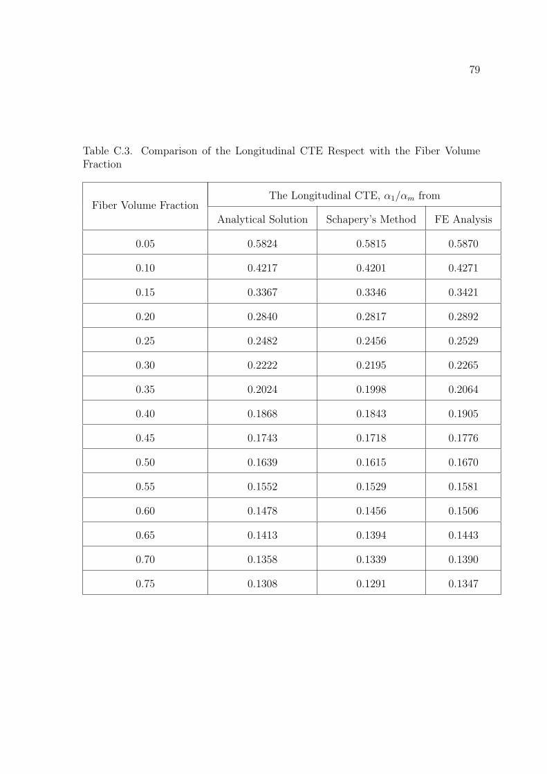
Table C.3. Comparison of the Longitudinal CTE Respect with the Fiber VolumeFraction

Fiber Volume FractionThe Longitudinal CTE, α1/αm from

Analytical Solution Schapery’s Method FE Analysis

0.05 0.5824 0.5815 0.5870

0.10 0.4217 0.4201 0.4271

0.15 0.3367 0.3346 0.3421

0.20 0.2840 0.2817 0.2892

0.25 0.2482 0.2456 0.2529

0.30 0.2222 0.2195 0.2265

0.35 0.2024 0.1998 0.2064

0.40 0.1868 0.1843 0.1905

0.45 0.1743 0.1718 0.1776

0.50 0.1639 0.1615 0.1670

0.55 0.1552 0.1529 0.1581

0.60 0.1478 0.1456 0.1506

0.65 0.1413 0.1394 0.1443

0.70 0.1358 0.1339 0.1390

0.75 0.1308 0.1291 0.1347

80

Table C.4. Comparison of the Transverse CTE Respect with the Fiber Volume Frac-tion

Fiber Volume FractionThe Transverse CTE, α2/αm from

Analytical Solution Schapery’s Method FE Analysis

0.05 1.0785 1.0891 1.0731

0.10 1.0583 1.0862 1.0571

0.15 1.0087 1.0564 1.0161

0.20 0.9473 1.0150 0.9655

0.25 0.8809 0.9675 0.9104

0.30 0.8128 0.9166 0.8535

0.35 0.7447 0.8634 0.7957

0.40 0.6777 0.8087 0.7376

0.45 0.6123 0.7529 0.6794

0.50 0.5489 0.6963 0.6209

0.55 0.4873 0.6392 0.5616

0.60 0.4277 0.5816 0.5009

0.65 0.3696 0.5236 0.4377

0.70 0.3127 0.4653 0.3702

0.75 0.2561 0.4068 0.2958

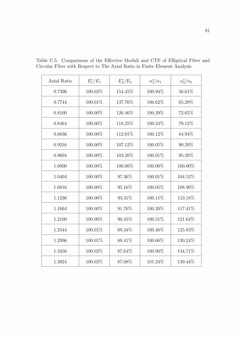
81

Table C.5. Comparisons of the Effective Moduli and CTE of Elliptical Fiber andCircular Fiber with Respect to The Axial Ratio in Finite Element Analysis

Axial Ratio E∗1/E1 E∗

2/E2 α∗1/α1 α∗

2/α2

0.7396 100.02% 154.45% 100.94% 56.61%

0.7744 100.01% 137.76% 100.62% 65.29%

0.8100 100.00% 126.46% 100.39% 72.65%

0.8464 100.00% 118.25% 100.24% 79.12%

0.8836 100.00% 112.01% 100.12% 84.94%

0.9216 100.00% 107.12% 100.05% 90.29%

0.9604 100.00% 103.20% 100.01% 95.28%

1.0000 100.00% 100.00% 100.00% 100.00%

1.0404 100.00% 97.36% 100.01% 104.52%

1.0816 100.00% 95.16% 100.05% 108.90%

1.1236 100.00% 93.31% 100.11% 113.18%

1.1664 100.00% 91.76% 100.20% 117.41%

1.2100 100.00% 90.45% 100.31% 121.64%

1.2544 100.01% 89.34% 100.46% 125.83%

1.2996 100.01% 88.41% 100.66% 130.24%

1.3456 100.02% 87.64% 100.90% 134.71%

1.3924 100.02% 87.08% 101.24% 139.44%

82

Table C.6. Comparisons of the Effective Moduli and CTE of Elliptical Fiber andCircular Fiber with Respect to The Axial Ratio in Analytical Solution

Axial Ratio E∗1/E1 E∗

2/E2 α∗1/α1 α∗

2/α2

0.7396 100.02% 154.04% 101.60% 65.78%

0.7744 100.02% 138.70% 101.27% 72.78%

0.8100 100.02% 127.79% 100.99% 78.79%

0.8464 100.01% 119.56% 100.75% 84.04%

0.8836 100.01% 113.12% 100.53% 88.69%

0.9216 100.01% 107.91% 100.33% 92.85%

0.9604 100.00% 103.61% 100.16% 96.60%

1.0000 100.00% 100.00% 100.00% 100.00%

1.0404 100.00% 96.91% 99.85% 103.11%

1.0816 100.00% 94.24% 99.72% 105.96%

1.1236 99.99% 91.91% 99.60% 108.59%

1.1664 99.99% 89.85% 99.48% 111.02%

1.2100 99.99% 88.02% 99.38% 113.27%

1.2544 99.99% 86.38% 99.28% 115.37%

1.2996 99.99% 84.91% 99.19% 117.34%

1.3456 99.99% 83.57% 99.10% 119.17%

1.3924 99.98% 82.36% 99.02% 120.90%

REFERENCES

[1] R. Kulkarni and O. Ochoa, “Transverse and longitudinal cte measurements of

carbon fibers and their impact on interfacial residual stresses in composite,”

Journal of Composite Materials, vol. 40, 8.

[2] H. G. Kia, “Thermal expansion of sheet molding compound materials,” Journal

of Composite Materials, vol. 42(7), pp. 681–695, 2008.

[3] R. A. Schapery, “Thermal expansion coefficient of composite materials based on

energy principles,” Journal of Composite Materials, vol. 2(3), pp. 380–404, 1968.

[4] B. W. Rosen and Z. Hashin, “Effective thermal expansion coefficients and specific

heats of composite materials,” International Journal of Engineering Science,

vol. 8, pp. 157–173, 1970.

[5] G. P. Tandon and A. Chatterjee, “The transverse coefficient of thermal expansion

of a unidirection composite,” Journal of Material Science, vol. 26, pp. 2759–2764,

1991.

[6] T. Ishikawa, K. Koyama, and S. Kobayashi, “Thermal expansion coefficients of

unidirectional composites,” Journal of Composite Materials, vol. 12, pp. 153–168,

1978.

[7] J. D. D. Melo and D. W. Radford, “Determination of the elastic constants of a

transversely isotropic lamina using laminate coefficients of thermal expansion,”

Journal of Composite Materials, vol. 36(11), pp. 1321–1329, 2002.

[8] J. S. Wang and W. S. Chan, “Effects of defects on the buckling load of rodpack

laminates,” Journal of American Helicopter Society, vol. 45, pp. 216–221, 2000.

83

84

[9] W. Yu and T. Tang, “A variational asymptotic micromechanics model for pre-

dicting thermoelastic properties of heterogeneous materials,” International Jour-

nal of Solids and Structures, vol. 44, pp. 7510–7525, 2007.

[10] M. R. Islam, S. G. Sjolind, and A. Pramila, “Finite element analysis of linear

thermal expansion coefficients of unidirectional cracked composite,” Journal of

Composite Materials.

[11] Z. H. Karadeniz and D. Kumlutas, “A numerical study on the coefficients of

thermal expansion of fiber reinforced composite materials,” Composite Struc-

tures, vol. 78, pp. 1–10, 2007.

[12] I. M. Daniel and O. Ishai, Engineering Mechanics of Composite Materials. New

York: Oxford University Press, 2006.

BIOGRAPHICAL STATEMENT

Nittapon Srisuk was born in Nakhon Nayok, Thailand, in August 1983. He

received his B.S. degree in Aeronautical Engineering from Royal Thai Air force

Academy, Thailand, in 2005. From 2005 to 2008, he was in the Air Technical Divi-

sion, Directorate of Aeronautical Engineering as an engineer. In 2008, he pursued his

master degree in Aerospace Engineering at The University of Texas at Arlington.

85

Documents

A MICROMECHANICS MODEL OF THERMAL EXPANSION …