A micro-powered model of mortgage default risk for full … · · 2016-04-25A micro-powered model of mortgage default risk for full recourse economies, with an application to the

IFC workshop on “Combining micro and macro statistical data for financial stability analysis. Experiences, opportunities and challenges”

Warsaw, Poland, 14-15 December 2015

A micro-powered model of mortgage default risk for full recourse economies, with an application to the

case of Chile1

Diego Avanzini, Juan Francisco Martínez and Víctor Pérez, Central Bank of Chile

1 This paper was prepared for the meeting. The views expressed are those of the authors and do not necessarily reflect the views of the BIS or the central banks and other institutions represented at the meeting.

A micro-powered model of mortgage default risk for

full recourse economies, with an application to the case

of Chile�

Diego Avanziniy

Central Bank of Chile

Juan Francisco Martínez


Víctor Pérez


October 21, 2015

Abstract

This paper develops a customized model of mortgage loans default for a full recourse

economy. We combine the more usual analysis for nonrecourse economies, adding a

non-pecuniary cost for defaulting in order to account for possible loss of utility due to

the full-recourse framework. This model applies to economies such as Spain, Australia,

and Chile, where defaulters can be prosecuted until their debts are completely settled.

Under the proposed model, we obtain an analytical expression involving default de-

terminants for mortgage loans, both micro and macro. As a case study, we estimate

�This paper has been prepared for the Workshop on Housing, Santiago, April 25, 2014, at the CentralBank of Chile. The views and conclusions presented in this paper are exclusively those of the authors and donot necessarily re�ect the position of the Central Bank of Chile or of the Board members. We are gratefulto Natalia Gallardo for helping us and contributing in a preliminary stage of this work. All errors are ourown.

yCorresponding author: [email protected], Statistical Division, Central Bank of Chile.

1

this relationship for the Chilean economy using information from the Chilean Survey

of Household Finance (EFH). As stated by our micro-macro model, we �nd that house-

hold �nancial conditions and their interactions with systemic determinants account for

an important part of the cross sectional probability of mortgage default.

Keywords: Default, Mortgage loan, Survey data, Full recourse economy, Rare

events, Credit market

JEL Classi�cation Number: C35, D53, E44, G21

2

1 Introduction

The recent �nancial crisis has tested the academics and regulators in their ability to anticipate

possible sources of instability. Some of the lessons that can be learnt from the latest �nancial

crisis is that policy models and their estimates should take into account factors that might

have been at some point overlooked. The recent experience suggests the existence of a

mortgage channel that acts as an accelerator or ampli�er element of �nancial instability.

This is why, for central banks and policy makers, it is crucial to understand the mechanisms

at place, and to use richer sources of data to measure them. Hence, in this work we contribute

to the existing literature by presenting a theoretical model that incorporates both micro and

macro �nancial determinants and their interactions for a full recourse economy. We apply

the framework to the Chilean economy as a case study, and test it empirically using using a

rich source of micro-data coming from the Chilean Survey of Household Finance.1

It is widely accepted in the current economic literature, that �in aggregate terms� a

mortgagor facing a negative equity is prone to default. In this case, when the value of debt

is higher than the value of the collateral, there are incentives to optimally decide not to

repay, since it is cheaper to give up the property and to stop repaying. This mechanism

is in the heart of various recent crisis related papers such as those of Fostel and Geanako-

plos (2008) and Goodhart et al. (2011). Other in�uential papers that model a collateral

�nancial economy are Kiyotaky and Moore (1997) and Bernanke et al. (1999), but instead

of households, these works model �rms dynamics under the presence of a credit market af-

fected by asymmetric information. In their settings, the risk premium depends on the �rms�

probabilities of default, which in turn are related to the value of net worth.

The model that inspires our treatment of the default phenomenon is developed in Geanako-

plos and Zame (2013).2 They abstract from the explicit modeling of asymmetric information,

1From now on "EFH", for its name in Spanish ("Encuesta Financiera de Hogares"). The survey isconducted by the Central Bank of Chile (BCCh) since 2007.

2Note that this is a published version of a working paper that was �rst issued in 1997.

3

but allow for an equilibrium with endogenous default. To do this, they base their model �

as all the theoretical literature in this �eld� on a non-recourse credit regulation policy.

Non-recourse regulatory frameworks state that the lender gets the collateral only after the

occurrence of a default and it is not allowed to prosecute other payments or compensations

from the debtor. In this way, modelers avoid the imposition of deadweight losses associated

to other punishments in case of default.3

However, when modeling the determinants of mortgage default for economies such as

Australia, Chile, and Spain, we need to introduce the case of full recourse regulation. Under

this type of regulation, agents can be prosecuted until their debts are completely settled. This

implies that the incentives to repay should be enhanced, since in a full recourse framework,

the incentive to default due to negative equity is counteracted by the fact that if the collateral

is not su¢ cient to cover the promises, the creditor has the right of going after other assets of

the debtor. There is also a reputational e¤ect given that the prosecuted debtors are publicly

listed. All these issues motivate us to develop a modeling alternative that adapts the seminal

framework of Geanakoplos and Zame (2013).

Economic intuition indicates that our model should incorporate a mechanism that ad-

ditionally discourages mortgagors from defaulting. This is consistent with the idea that

mortgagors do not always default when they face negative equity on their homes as in Har-

rison et al. (2004) or Ellul et al. (2010). In fact, Foster and Van Order (1984) and Bhutta

et al. (2010) �nd that many borrowers with negative equity do not default; and, conversely,

default is often associated with shocks, such as unemployment. Also, the cost of continuing

to repay a mortgage also depends on the agent�s idiosyncratic discount factor and thus on

his liquidity position, as Elmer and Seelig (1999), Gerardi et al. (2007), and Bajari et al.

(2010) explain.

Our model formulation closely follows part of the Goodhart et al. (2011) work, which

3As Geanakoplos and Zame (2013) state, the only seizure of collateral "[...] avoids the moral and ethicalissues of imposing penalties in the event of bad luck." Although, they recognize that in practice, the seizureof collateral implies deadweight losses on its own.

4

is a recent application based in the Geanakoplos and Zame (2013, and the earlier work

dated 1997) model. Yet, in order to modify the mortgage default incentives, we add a non-

pecuniary cost that arises as a reputational loss because of the burden of being enforced to

repay the debt and other possible losses of utility (e.g. being blacklisted from the credit

market or being banned for future credit opportunities). Natural references that we consult

to address this type of default cost are those of Shubik and Wilson (1977) and Dubey et

al. (2005). Together with Geanakoplos and Zame (2013), these works lie within the general

equilibrium literature. Our contribution consists in combining both frameworks to generate

a full recourse economy, such as that of Spain, Australia and Chile.

To test our framework, we apply it to the Chilean case. The literature that models default

decisions in the Chilean economy is rather brief. One of the recent investigations appears in

Alfaro and Gallardo (2012). These authors estimate an empirical characterization using the

EFH 2007 survey. They �nd that income and income-related variables are the only signi�cant

and robust factors that explain default for both types of debt (consumer and mortgage).

Additionally, demographic variables can help to further explain default probabilities.

Empirical evidence suggests that there is some rich information hidden away in aggregated

(or macro) data. Thus, the use of micro-data seems a promising research avenue. That is why,

instead of using �nancial aggregates of credit and macro-�nancial conditions to determine

default dynamics through time, we follow Alfaro and Gallardo (2012) in the sense that we

use micro-information coming from the EHF survey. As compared to the latter, beyond

contributing with a theoretical modeling framework, in this work we are able to pro�t from

the additional information that the EFH survey has gathered through the years since it was

launched in 2007.

The main objective of this work is to improve the identi�cation and estimation of default

determinants in the mortgage market. Our results can contribute to support credit policy

measures and also enhance the analysis and application of mortgage banking stress tests. In

particular, we apply this methodology to the Chilean economy, but it may be relevant to

5

other countries, such those already mentioned.

In recent years, theoretical advances and economic necessity have stimulated the study

of the default decision specially on mortgage loans. Since Kau et al. (1994) and Capozza

et al. (1997), theoretical models and empirical testing have being integrated in the search

for a better understanding of the phenomenon. Following those e¤orts we elaborate on the

theoretical modeling of mortgage default and estimate the resulting model using microdata

from households in Chile.

The rest of the work is organized as follows. Section 2 introduces the theoretical model.

Section 3 highlights the role of the determinants as they emerge from the model. In Section

4 we describe the empirical methodology as well as the dataset we use for the estimations.

All the results are presented in Section 5. Some �nal remarks are in Section 6. The Appen-

dix contains derivations and proofs from the model, a supporting glossary, and some data

description.

2 A theoretical model of the determinants of default

To provide a general view of the mortgage default mechanism at play, in this section we

introduce and describe a partial equilibrium model that motivates our empirical estimations.

We describe the economy, agents, �nancial structure, transactions and its timing.

Our model considers a two-period setup. The beginning (t = 0) is deterministic, but the

second period (t = 1) is stochastic. In the latter, there are s possible states of nature that

occur with probability �s.4 To help notation, we also de�ne S = f0; sg, a t�uple that groups

both periods and consider the possible states at the second period.

The economy is composed by one representative household. There are two goods traded

in this economy: a consumption commodity and housing. We also have two types of �nan-

cial assets: one short-term (intra-period) unsecured loan and one long-term (inter-period)

4Later we will specify that state variables are in our case represented by commodity endowments andliquidity conditions (i.e. interest rates and monetary endowments).

6

collateralized loan.

The household is endowed with a perishable commodity that consumes and sells, and

money. The endowment is deterministic in the �rst period, and depends on the realized

state of nature in the second period. The agent also consumes housing in both periods

that has to be purchased. There are two di¤erences between commodities and housing. On

the one hand, commodities are perishable (they only provide utility in the period they are

available) while durable goods (house) purchased at the initial period (t = 0) also give utility

at the �nal one (t = 1). On the other hand, housing also serves as collateral when contracting

a long term loan.

2.1 Financial intermediation

The �nancial intermediation in this model is assumed to be exogenous and it is treated

in a stylized manner. However, it can be thought of as a representative bank (or banking

system) that lends short-term to the representative household,5 as well as an inter-period

collateralized mortgage loan. The latter is only available at t = 0. An exogenous amount of

liquidity is pumped into the system and it is re�ected in the short- and long-term interest

rates (rS and �r; respectively).6 Nominal �ows of the economy are depicted in Figure 1.

2.2 Timing

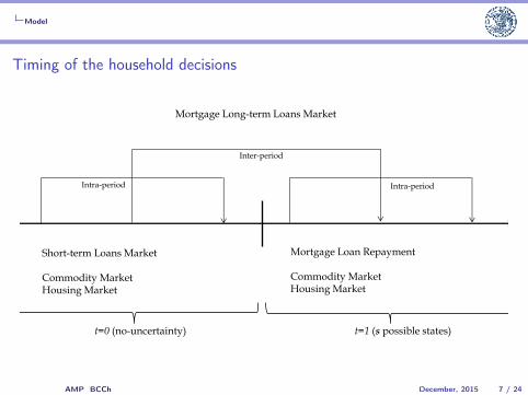
At the initial period (t = 0) short-term liquidity borrowing plus long-term mortgage bor-

rowing from the representative household occur. Provided the �nancing, transactions in

commodity and mortgage markets take place. The representative agent sells part of his

endowment of the consumption commodity and uses the revenues to repay the short-term

loan obligations. Under the current setup, short-term obligations arise as a consequence of

5To help the focus of the analysis and without loss of generality, this type of loan is assumed to bedefault-free.

6It can be thought of as the monetary authority that injects certain amount of resources in the moneymarket, in�uencing the short-term rates (e.g. through MS) and long-term interest rates (e.g. through �M).

7

the assumption of a cash-in-advance �nancial economy. The agent also purchases housing,

which is �nanced with a collateralized long-term mortgage loan. Finally, consumption of

housing and commodity takes place.

During the second period (t = 1) the nature realizes and reveals s, which mainly a¤ects

endowments �including monetary� and monetary supply, as we observed before. At this

period, the intra-period transactions work in a similar manner than at the beginning. How-

ever, there are slight, but signi�cant di¤erences. First, it is easy to see that the long-term

interest rate is already �xed (e.g. because the long-term money market does not open at

every period). Second, the mortgage loan is settled by the representative household, given

by his delivery (or default) decision. At this period, he uses the short-term money market

to repay the long-term loans and �nances his housing consumption.

2.3 Economy and budget set

The economy is composed by a positive endowment of the perishable commodity, eS1;

positive monetary endowment mS; preferences U ; �nancial assets consisting of long

and short-term loans at rates �r and rS, respectively. We assume that in this economy

preferences are monotonic and utility is quasi-concave.

Given a set of securities (i.e. short and long-term loans) �; commodity price pS1; housing

price pS2; rate of return of the short and long-term credit market rS and �r, respectively; the

mortgagor with commodity endowment eS1 makes consumption plans, credit demand, sales

of commodity, and deliveries against promises.7 Following Geanakoplos and Zame (2013), in

the case of mortgages, optimal deliveries will be always the minimum of promises (i.e. credit

demand) and the value of the collateral. Thus, we de�ne the budget set for the representative

household as B (p1; p2; rS; �r; eS1;�) to be the set of plans (�; ��; qS1; bS2), where � stands for

the short term borrowing, �� is the mortgage borrowing, qS1 represents the commodity sales

7Our notation for prices, quantities and monetary expenditures contains a subindex with two components.The �rst one is the period (or state at t = 1), while the second term indicates the type of good, 1 forcommodities and 2 for housing.

8

and bS2 stands for housing expenditure.

We have that at the initial date (t = 0), the agent is subject to three budget constraints.

First, the short term loans must not exceed the revenues from commodity sales. Second,

the housing expenditure must be lower than or equal to its long and short term credits and

monetary endowment. Finally, the third constraint considers an element of mortgage credit

regulation. There is a �xed portion of collateral (i.e. �) required for a mortgage loan.8

Formally, we have that, at t = 0 :

�0 � p01q01

b02 � �01 + r0

+��

1 + �r+m0

��

1 + �r� �b02

Conversely, at the �nal date (t = 1), the agent is subject to two budget constraints.

The �rst constraint re�ects the fact that the short term loans must not exceed the revenues

from commodity sales. The second budget constraint depends on the state of nature that is

realized. Thus, under a good state of nature (i.e. s 2 SG, where no default is exerted), the

constraint states that the repayment of the mortgage loans plus the new housing consumption

of the household (i.e. a type of housing top-up) must not exceed the agent�s short-term

borrowing and monetary endowment. Under a bad state of nature (i.e. s 2 SB, there is

default), the constraint accounts for the fact that there is no mortgage repayment.

Formally, at t = 1; the constraints are:

�S � ps1qs1

bs2 + �� s1 + rs

+ms 8s 2 SG

bs2 � �s1 + rs

+ms 8s 2 SB

8Without loss of generality, we assume that this constraint is always binding in equilibrium.

9

2.4 Preferences

At the beginning of the time (t = 0), the representative household maximizes his expected

utility subject to the budget constraints previously described. The agent�s utility in our

case has the particularity that default incentives are mitigated by seizing the collateral of

the mortgagor.9 However, to adequate the problem to a full recourse economy, we also

introduce a non-pecuniary default penalty proportional to the defaulted amount, similar to

Shubik and Wilson (1977) and Dubey et al. (2005). Thus �subject to his budget set�, the

agent solves the following program:

max�s;��;bs2;qs1

U = u (e01 � q01) + u�b02p02

�+Xs2S

�s fu (es1 � qs1)g+

+Xs2SG

�s

�u

�b02p02

+bs2ps2

��+Xs2SB

�s

�u

�bs2ps2

��

��Xs2S

�smax

��1� b02ps2

p02��

�; 0

�

That is, the agent optimizes his utility function, by solving his plan of short and long-

term borrowing, housing expenditure (in monetary terms) and commodity sales (quantity),

subject to his budget constraints. At the �rst period (t = 0), the agent obtains utility

from consuming the commodity that remains from his sales and the housing units that he

purchases. At the �nal period (t = 1), the representative household faces the two possible sets

of states of nature, good or bad. If a good state realizes, there is no default. Thus, the agent

enjoys from consuming his initial date housing consumption plus the additional housing

he buys in the �nal period. Conversely, if the household faces a bad state of nature, he

(optimally) defaults.10 In such cases, the (non-modelled) banking sector seizes the collateral,

so the agent cannot bene�t from consuming the initial period housing and he is subject to

9We interpret this as an exogenous commercial banking sector that is compensated by receiving thecollateral. In turn, it sells it back into the market to cash-in.10As we previously mentioned, the optimal delivery is the minimum between the current value of collateral

and the promises (i.e. min f��; (b02ps2=p02)g).

10

a default penalty (linearly) proportional to the defaulted amount. It has to be noted that

in this model, the agent is not expelled from the market. He is still allowed to obtain short

term credit.11

2.5 Equilibrium

This section provides a brief note on equilibrium. From the problem formulation, we have

that this economy is composed only by the representative household. Here we assume that

he behaves in a competitive manner, so takes prices as given.

The competitive collateral equilibrium (CCE) in this economy consists of a set of com-

modity prices (pS1), security prices (interest rates rS, �r) and consumption plans (�; ��; qS1; bS2),

such that short-term commodity market clears, durable housing market clears, security mar-

kets clear, plans are budget feasible and consumers optimize.

There are important particularities to be highlighted in this type of economy. On the one

hand �in this partial equilibrium model�, we abstract from a housing pricing ampli�cation

mechanism �rst described by Fisher (1933) and, more recently, by Goodhart et al. (2011).

In these works, if a bad state is attained and there is mortgage default, the representative

household will have to give-up the collateral and the housing goes back to the market. In

such a situation, the housing market clearing condition incorporates that there is a decrease

in prices that further increase default incentives, given that collateral losses value, and the

debt face value remains. This spiral-type mechanism is called debt-de�ation.

Another issue to be considerer concerns to rational expectations. In this work we also

abstract from explicitly modelling the �nancial (banking) sector. Thus, we do not need to

consider the rational expectations of the lending activity. Nevertheless, in cases where the

banking sector appears (e.g. Goodhart et al., 2011), and to incorporate the default possibility

under rational expectations, the e¤ective return on the mortgage will be the ratio between:

(i) the minimum between the collateral value at t = 1 and the mortgage promise, ��; and (ii)

11The agent�s program �rst order conditions appear in the Appendix.

11

the initial mortgage extension (credit supply). That is, a bank should rationally anticipate

the optimal household delivery and account for this into the risk premium.

Theorem 1 Existence: Assuming rational expectations, a well-behaved (e.g. normally dis-

tributed) state probability space, monotonic preferences, quasi-concave utility (quasi-concavity

is assumed to be maintained in the presence of linear penalties) and convex budget sets, and

provided that all the markets clear, this economy admits a competitive equilibrium.

Proof. It appears in Geanakoplos and Zame (2013).

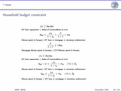
3 Determinants of mortgage default

Proposition 2 Existence of full-recourse determinants of mortgage default: From the house-

hold optimization problem solution, and assuming without loss of generality that there are

only two possible states of nature (the good G, where there is full delivery, and the bad B,

where there is default) we can obtain an equation that represents the mortgage default deter-

minants. Furthermore, the default depends on idiosyncratic and systemic factors as well as

their interactions. The explicit equation is given by:

1� b02pB2��p02

= !0 + !1��u0�b02p02

�+ !2��u

0�b02p02

+bG2pG2

�+ !3��u

0 (e01 � q01) (1)

where

!0 = 1� ��BpB2p02(1 + �r)�

!1 = � 1

p02��B (1 + �r)�

!2 =�G (�p02 (1 + �r)� pG2)pG2p02��B (1 + �r)�

!3 = � (1 + r0) (1� �)p01��B (1 + �r)�

12

Proof. See the Appendix.

Notice that the left hand side of equation (1) corresponds to the expected default fre-

quency on the mortgage loans (i.e. the complement of the expected repayment). The right

hand side is composed by systemic and idiosyncratic factors, and their interactions. All of

them constitute the determinants of mortgage default.

Remark 3 Systemic factors: Notice that !0, the �rst term at the RHS of equation (1)

accounts for the banking regulation and �nancing standards faced by the household. This

is a systemic factor that a¤ects households independently from their idiosyncracies (i.e. it

is exogenous to them). It is easy to see that the default frequency decreases with: (i) a

higher default penalty, (ii) a lower LTV (�), (iii) a higher interest rate, and (iv) a decrease

in housing prices. Our interpretation is consistent with Ja¤ee and Stiglitz (1990) that the

higher the screening, the lower the default incentives. On the other hand, a tighter regulation

provides lower incentives to default, as in OECD (2011). Additionally, the terms !1, !2 and

!3 depend only on exogenous variables or parameters. Thus, they also work as exogenous

systemic factors that interact with agent�s idiosyncracies.

Remark 4 Systemic and idiosyncratic interaction �housing and mortgage demand in the

�rst period: The second term at the RHS of equation (1) shows a systemic factor interacted

with credit demand and marginal utility of housing at t = 0. Given that !1 is always nega-

tive, we interpret that the higher the marginal utility of housing consumption and mortgage

demand, the lower the incentives to default. Alternatively, given that we assume that pref-

erences are quasi-concave, the higher the preference for housing consumption, the higher the

expected mortgage default.

Remark 5 Systemic and idiosyncratic interaction �housing and mortgage demand in the

second period: The third term at the RHS of equation (1) also contains the systemic factor

interacted with the marginal utility, but in this case it is in the good state at t = 1. The

systemic factor !2 in this case has an ambiguous sign. It is easy to see that if prices are in

13

a growing phase12 (i.e. p02 < pG2) and credit supply standards are su¢ ciently relaxed (i.e.

� (1 + �r) > 1), then the dynamics of mortgage default and housing demand work in the same

direction than in the second term of (1).13 To sum up, under the speci�ed conditions, higher

mortgage or housing demands are associated to greater expected defaults.

Remark 6 Systemic and idiosyncratic interaction - income: The fourth term at the RHS of

equation (1) works in a similar fashion with regard to the systemic component. There is a

negative relationship between tighter (short-term) credit standards and mortgage default prob-

abilities. The e¤ect is proportional to the ratio between the housing and commodity current

prices.14 This result is conditioned on the marginal utility of consumption. Assuming risk

aversion (e.g. logarithmic utilities), we have that �for a given mortgage credit standard and

prices ratio�the higher the commodity endowment, the lower the mortgage default frequency.

In this case, we interpret endowments as the availability of resources. Thus, it expresses the

importance of housing income in this context. Our conjecture is that the combination of

systemic credit standards and household income (or a related variable) is key to determine

mortgage default frequency.

From the �ndings that our theoretical model provides, we conjecture that mortgage

default determinants are associated to credit cost and/or regulation standards and its inter-

action with idiosyncratic factors, such as the demand for housing and income. At this point,

it is important to notice the interaction that we found. This will be key in our empirical

speci�cation which will be based on our theoretical model results.

4 Estimation Methodology and Data

In this section we brie�y describe the problems that we face to obtain unbiased and e¢ cient

estimators, and the characteristics of the data used in the estimations.

12This ensures that the good state is attained.13This is straightforward if we notice that !2 = !1pG2�G.14This is easy to see if we notice that !3 = !1 (p02=p01) (1 + r0) (1 + �) :

14

4.1 Estimation Methodology

In this work we explain the default decision of households on their mortgage loans based on

idiosyncratic and systemic variables. For doing this, we use logistic regressions to estimate

the behavior of a discrete variable representing the fact that some households in our sample

have defaulted their mortgages.

Our data on mortgage delinquency present two important features we need to account

for in the estimation. First, defaulting a loan (specially mortgages) is not an usual event.

Futhermore, it can be considered as a rare event when compared with the occurrence of the

contrary. Thus, if we take into account the whole population of outstanding mortgage loans

in an economy, delinquency is highly underrepresented in any sample. However, our sample

captures an important mass of delinquent loans in order to better appreciate its behavior.

This means that the sample is intentionally biased to account for the phenomenon. This

is known in econometrics as choice-based or endogenous strati�ed sampling. This sampling

method is often supplemented with known or estimated prior knowledge of the population

fractions of the rare event (as in our case).

Second, popular statistical procedures including the logistic regression, can sharply un-

derestimate the probability of rare events. As King and Zeng (2002) point out, that logit

coe¢ cients are biased in small samples is well documented in the literature, but that in rare

events data the biases in probabilities can be substantively meaningful is less known and un-

derstood. In particular, �nite sample, rare event data have at least three features we should

account for: (i) increasing the size of the sample does not alleviate the bias, because the rare

events do not increase their share of the sample more quickly than the growth rate of the

sample; (ii) the bias of the coe¢ cients estimated using logistic regression when rare events

are present is known to underestimate the probability of the rare event; (iii) the computation

of probabilities of events in logit analysis is suboptimal in �nite samples of rare events data,

leading to errors in the same direction as biases in the coe¢ cients.

15

To deal with these features together, we follow the developments of King et al. (2000) and

King and Zeng (2001, 2002). Assume that we have a dataset of i = 1; :::; n observations for

which we have gathered information on the variable Yi and a set of k� 1 variables recorded

in xi: The variable Yi is a dicothomous variable that represents an underlying continuous

variable Y �i following Yi = 1 if Y �i > 0 and Y i = 0 if Y �i � 0: Yi follows a Bernoulli

distribution, while Y �i follows a Logistic distribution. The behavior of Y�i can be adequately

inferred from the maximum likelihood estimation of the behavior of Yi.

We assume that the ones (Yi = 1) are the rare outcome, representing those households

that hold a delinquent mortgage loan. The prior population information refers to the fraction

of ones in the population, � , while the observed fraction of ones in the sample refers to the

sampling probability, y.

To compensate for di¤erences in the sample (y) and population (�) fractions of ones

induced by choice-based sampling we use a weighting procedure. The procedure maximizes

the weighted log-likelihood:

lnLw(�jy) = w1XfYi=1g

ln(�i) + w0XfYi=0g

ln(1� �i)

= �nXi=1

wi ln (1 + exp [(1� 2Yi)xi�]) (2)

where the weights are w1 = �=y and w0 = (1� �)=(1� y), and where

wi = w1Yi + w0(1� Yi)

The resulting �̂ is the weighted exogenous sampling maximum-likelihood estimator, due to

Manski and Lerman (1977). One of the advantages of this method is that weighting can

outperform other approaches (e.g. prior correction) when both a large sample is available

and the functional form is misspeci�ed (see Xie and Manski, 1988). However, weighting

is asymptotically less e¢ cient in small samples (see Scott and Wild, 1986; Amemiya and

16

Vuong, 1987).

When information about � is available, we can remedy these problems using an analytical

approximation to the bias based on McCullagh and Nelder (1989). The bias in �̂ can be

estimated by the following weighted least-squares expression:

bias��̂�= (X0WX)

�1X0W�

where �i = 0:5Qii[(1 + w1)�̂i � w1], Qii are the diagonal elements of Q = X(X0WX)�1X0,

and W = diagf�̂i(1� �̂i)wig. The bias-corrected estimate is then

~� = �̂ � bias��̂�:

Notice that this correction a¤ects the constant term directly, but also the other coe¢ cients

primarily as a consequence (King and Zeng, 2001).

The variance of the approximately unbiased estimate of �; ~�; is approximated by a

multiple of the usual variance matrix,

V�~��=

�n

n+ k

�2V��̂�:

A key point is that since (n=(n + k))2 < 1, V�~��< V

��̂�. Thus, reducing the bias also

reduces the variance.

4.2 Data Description

The primary source of information for our estimations is the Chilean Survey of Household

Finance (EFH). The EFH is an initiative of the Central Bank of Chile to collect information

about the household�s �nance including socioeconomic characteristics, information about

assets holdings, and detailed information on the debts of each household member. We use

the �ve available waves of the EFH: the �rst wave (2007) collected information from 3828

17

urban households at the national level; the second (2008), third (2009), and fourth (2010)

waves accounted for 1154, 1190, and 2037 urban households in the Metropolitan Region of

Chile, respectively; �nally, the �fth wave (2011-12) collected information from 4059 urban

households at the national level.

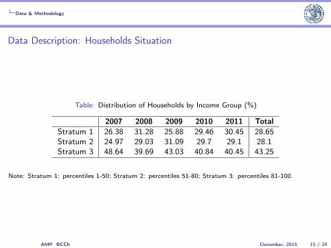
For each wave, higher income households have been oversampled in order to obtain a

better insight of the indebtedness. In Table 1 we show the percentage of households per

income stratum.15

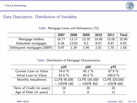
Table 2 shows information about mortgage holdings and delinquency as it comes from

the EFH. However, to correct the bias induced by rare events, we also incorporate some prior

information coming from the delinquency reported by the banks to the Superintendency of

Banks and Financial Institutions (SBIF, for its name in Spanish) every month. Ideally we

would use the number of delinquent loans versus the total number of outstanding loans.

However, that information is not available. Instead, we use the amounts of loans. Thus,

the prior information for us is given by the average ratio of the amount of nonperforming

mortgage loans to the total amount of outstanding mortgage loans in the Chilean �nancial

system, during the months each wave of the EFH was collected. Although imperfect, this

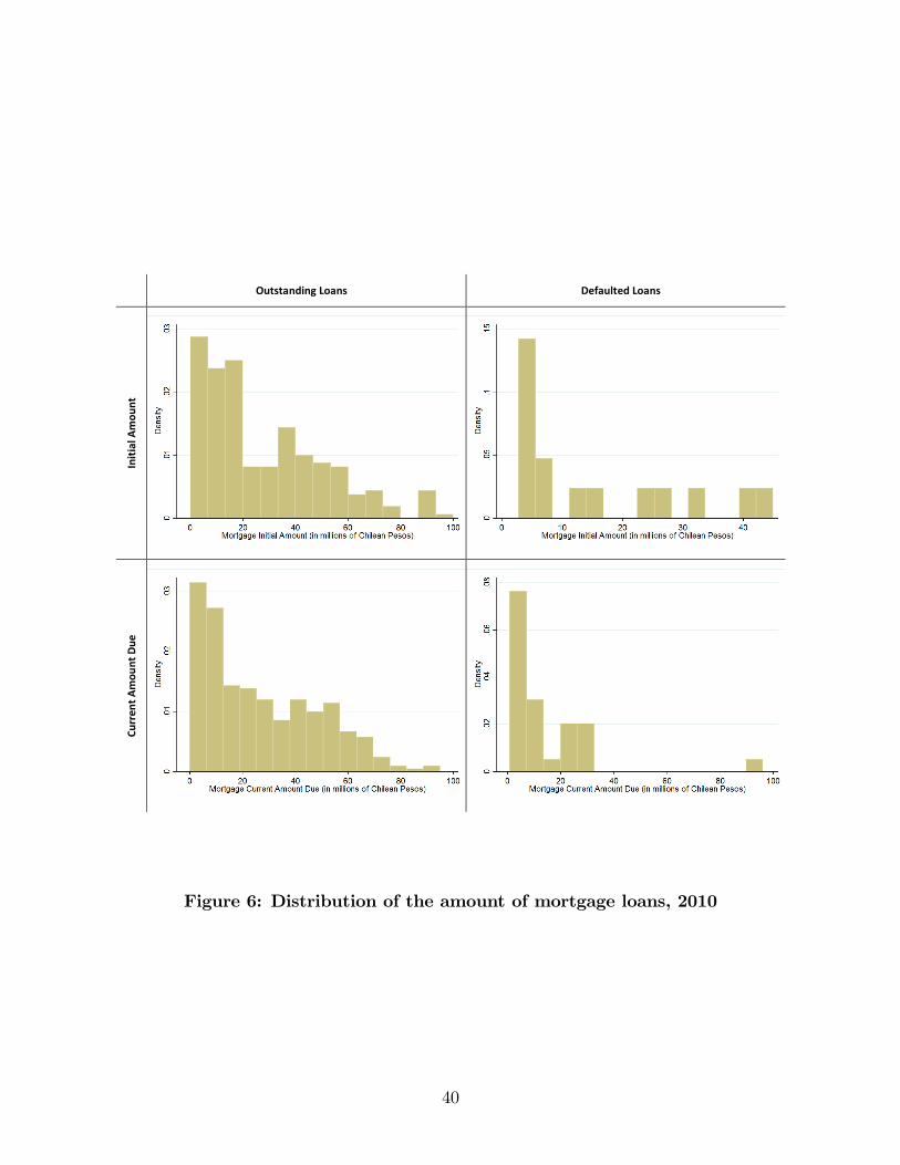
measure is a good approximation given the almost even distribution of the amount of credits

in delinquency in each wave of the EFH (see the Appendix for charts showing the distribution

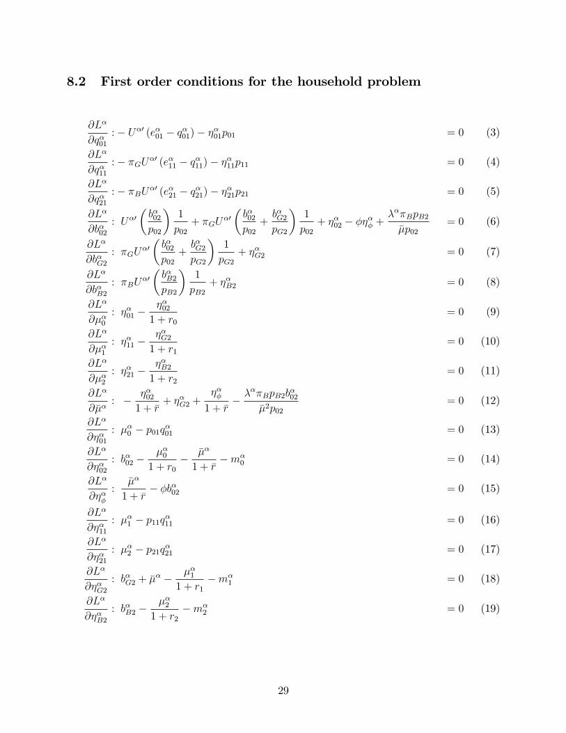
for each year). Notice that while the oversampling of defaulted loans is similar in the EFH,

the delinquency rate (as reported by the SBIF) changes over time following the impact of

the global crisis in Chile.

The EFH collects information on various aspects of the credits, but speci�c variables for

our estimations must be constructed. For each mortgage loan, we constructed the loan-to-

value ratio (LTV) for both initial loan amount and current outstanding debt. While most

of the analysis uses the initial LTV (eg. Kau et al., 1994; Harrison et al., 2004; Bajari et al.,

2010, 2012; Bhutta et al., 2010; Campbell and Cocco, 2010; Elul et al., 2010; Paniza Bontas,

15Stratum 1: percentiles 1-50; Stratum 2: percentiles 51-80; Stratum 3: percentiles 81-100.

18

2010; Hatchondo et al., 2012), we are more prone to use the current LTV (as in Capozza

et al., 1997, 1998; Ambrose and Capone, 1998; Wong et al., 2004). Our perspective is that

the current LTV better re�ects the �nancial burden for the household and is the appropiate

measure for the household to include in his optimization problem to evaluate the default

decision. The initial LTV is useful when the loan is in its �rst stages of payment, or when we

want to evaluate the risk involved at the time of granting the loan. However, for long-term

credits such as mortgages, the changing nature of the economic context and the household

�nancial balancesheet hinder the usefulness of the initial LTV. Nevertheless, in our analysis

we tested the role of both measures, as shown in the next section.

In Table 3 we present information on the quartiles of the current and initial LTV, and

the monthly installment. The median mortgage loan in our sample was granted to cover the

85% of the home value, and the current due amount represents the 45% of the current home

value. The median monthly installment is about $185,000 (around US$ 350). Also notice

that the median term of the credit is 20 years, while the median age of the credit (the time

period elapsed from the granting of the mortgage) is 6 years. As it can be seen, most of

the credits are granted for a term of around 20 years, while in more advanced economies the

usual term is around 30 years.

We make a �nal note on the situation of renegotiated mortgages to have some insight on

the behavior of those mortgagors that might be observed as defaulting but have renegotiated

the loans to avoid default. In our complete sample (12,268 households) we have that 15.9%

of them have an outstanding mortgage loan. Of them, the 19.5% have renegotiated the

conditions of their loans at some point. Table 4 shows default situation of mortgagors that

have renegotiated their loans. It is important to notice that there is a di¤erence between

households that are defaulting and those that are paying their debts after renegotiating a

mortgage: the main motivation to renegotiate for defaulters was "to decrease the mortgage

payment by increasing the term"; for those who kept paying their loan after renegotiation,

19

the main motivation was "a decrease in the interest rate".16

5 Results

In this section we present estimation results using the method described in the previous

section.17 There are two sets of estimations in the following tables. In Table 5, each idio-

syncratic and systemic variable enters directly in the regressions to explain the decision of

defaulting. In Table 6, there are interactions between these variables included as regressors

in the estimation, as suggested by our theoretical model.

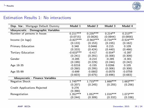
In Table 5, we show four di¤erent models that di¤er in the inclusion of �nancial idiosyn-

cratic variables and systemic variables. The set of demographic variables remain the same

for all estimated models. Notice that the sign, magnitude, and signi�cance of the coe¢ cients

accompanying the latter set of variables is stable through model speci�cations. Income is

an important determinant of the probability of default, and it enters the regressions with

the expected negative sign. Contrary to popular intuition, the number of persons in the

household impacts positively in the probability of default. This result may be associated

with the fact that in most cases at hand, a more densely populated household is not directly

associated with higher household total income (for example, because the increased number

of members of the household is due to the presence of children).

Regarding the �nancial variables, we �nd that su¤ering a negative shock in the recent

past signi�cantly increases the probability of defaulting a mortgage loan.18 Households that

renegotiated the conditions of their loans also are more likely to default them. Having

rejected credit applications appears not to be signi�cant to explain default behavior.16The distinction of motivations is based on an speci�c question for mortgagors that have renegotiated

their loans conditions, as collected by the EFH.17We have performed a complete set of estimations including a wide range of variables that were included in

previous empirical analysis of mortgage default. We also tried single step and two step estimations to correctfor possible endogeneity in the decision of getting a loan and then defaulting, as in Alfaro and Gallardo (2012).We did not �nd any technical or empirical reason to keep the track of the two step estimation procedure.However, all the additional results are available from the authors upon request.18The EFH collects information on a speci�c question that inquires about the occurrence of an event that

signi�cantly lowered the income o increased the expenditure and that was not planned.

20

We included three variables capturing systemic impact on household default behavior.

The current loan to value (CLTV) implies that a bigger CLTV increases the probability

of default all other things equal. Our results indicate that a higher amount due (higher

long-term �nancial burden) may impact positively the decision of defaulting (as in Elul et

al., 2010). On the other hand, higher price houses (usually associated with higher amounts

of loans) lessen the probability of default. The LTV of origination does not have major

impact on the decision of default. This result supports our argument that CLTV is the

relevant information for the household, specially if the relatively more defaulted loans are

the older ones. The systemic variables as a whole tell us that bigger mortgage loans are less

likely to default. These credits have being predominantly granted since 2005, accompanying

important aggregate phenomena of the Chilean economy: a sustained high growth period

(even during the global crisis), and a real estate boom. These two aspects require more

detailed analysis in terms of the risk-taking decision of the �nancial system and the aggregate

push-pull e¤ect of commodity prices and other macro determinants, all of them far beyond

the scope of this paper.19

The second set of results is presented in Table 6. Idiosyncratic demographic and �nancial

variables, as well as systemic variables, play a similar role to that of the results in Table 5.

The novel results come from the interaction between systemic and idiosyncratic variables, as

our theoretical model suggested. We �nd that the interaction between income and current

loan to value positively impact the chances of making default, as well as the interaction

between the price of the home at the origination moment and the fact that the household

su¤ered an unexpected negative shock. In the �rst case, even when the income has a negative

e¤ect on the default probability, the CLTV dominates in the overall. In the second case,

the e¤ect of the negative shock dominates the scene. These results emphasize that shocks

a¤ecting income (expenditure) or the remaining (long term) �nancial burden are key aspects

when analyzing default probabilities. For example, sustained high unemployment rates may

19Our general equilibrium framework incorporates these two levels of analysis together with the partialequilibrium we are presenting in this paper.

21

impact income level con�guring at the same time an unexpected shock that aggravates the

�nancial burden.

As we have analyzed above �and in contrast to Alfaro Gallardo (2012), which also analyze

the Chilean mortgage market�, the current LTV (CLTV) as a systemic factor is statistically

and economically signi�cant, as well as the house price at origination. This suggests that

both idiosyncratic and systemic factors (and its interactions) are simultaneously determining

the mortgage defaults.

6 Final Remarks

In this paper we propose a theoretical framework to model mortgage default in full re-

course economies. In such framework, it is possible to derive an analytical expression for

the household�s default decision that involves idiosyncratic and systemic factors, and their

combinations.

To empirically test this framework, we take into account two important issues of the

type of phenomenon we are studying: �rst, its occurrence is rare; and second, the sampling

framework favored the collection of data on default cases but contributes to worsen the

statistical properties of estimators. Overall, traditional logistic regression provides biased and

ine¢ cient estimators. We overcome this problem adopting appropiate adjustments suggested

by the literature.

Following our theoretical default description and the empirical strategy, we estimate the

default decision determinants for the representative Chilean household, using information

from the EFH survey.

According to our theoretical model, we �nd empirically that systemic and idiosyncratic

factors are statistically important to determine the default decision. Moreover, the systemic

and idiosyncratic interactions play a key role in determining default probability.

Our results suggest that aggregated macro�nancial variables �such as prices and loan to

22

value ratios�and its interaction with microeconomic information, can contribute to explain

an important portion of mortgage risks. This in turn implies that, when assessing the qual-

ity of a mortgage, or any other credit portfolio, the use of microeconomic or demographic

information is not enough. Accordingly, �nancial regulators and supervisors should invest

in developing aggregated measures that can act as early warning indicators, as well as incor-

porating market trends information into the analysis of risks. Furthermore, this constitutes

another rationale that reinforces the idea that monetary and banking authorities should in-

form the market about this type of �nancial developments in a consistent and integrated

report, that uses macro and micro �nancial information. Financial stability reports appear

as natural channel to issue this information.20.

7 References

Alfaro, R., and N. Gallardo (2012). �The Determinants of Household Debt Default,�Re-

vista de Análisis Económico �Economic Analysis Review, Ilades-Georgetown Univer-

sity, Universidad Alberto Hurtado/School of Economics and Bussines, 27(1)55-70.

Ambrose, B. W., and C. A. Capone (1998). �Modeling the conditional probability of

foreclosure in the context of single-family mortgage default resolutions,�Real Estate

Economics 26(3):391-429.

Amemiya, T., and Q. H. Vuong (1987). �A Comparison of Two Consistent Estimators in the

Choice-Based Sampling Qualitative Response Model.�Econometrica 55(3):699�702.

Bajari, P., S. Chu, and M. Park (2010). �An Empirical Model of Subprime Mortgage

Default from 2000 to 2007,�mimeo.

20Although the �nancial stability reports were developed and published �rst in the mid 2000�s, theyincreased their importance after the global �nancial crisis in 2008. Various central banks have developedtheir own periodic reports, such as UK, US, Spain, Australia, and Chile.

23

Bajari, P., S. Chu, D. Nekipelov, and M. Park (2012). �A Dynamic Model of Subprime

Mortgage Default: Estimation and Policy Implications,�mimeo.

Bernanke, B. S., M. Gertler, and S. Gilchrist (1999). �The �nancial accelerator in a quan-

titative business cycle framework,� Handbook of Macroeconomics, chapter 21, pp.

1341-1393.

Bhutta, N., J. Dokko, and H. Shan (2010). �The depth of negative equity and mortgage

default decisions,�Finance and Economics Discussion Series (FEDS) 2010-35, Divisions

of Research & Statistics and Monetary A¤airs, Federal Reserve Board (USA).

Campbell, J. Y., and J. F. Cocco (2010). �A Model of Mortgage Default,�mimeo.

Capozza, D. R., D. Kazarian, and T. A. Thomson (1997). �Mortgage default in local

markets,�Real Estate Economics, 25(4):631-655.

Capozza, D. R., D. Kazarian, and T. A. Thomson (1998). �The conditional probability of

mortgage default,�Real Estate Economics, 26(3):359-389.

Dubey, P., J. Geanakoplos, and M. Shubik (2005). �Default and Punishment in General

Equilibrium,�Econometrica, 73(1):1-37.

Elmer, P. J., and S. A. Seelig (1999). �Insolvency, trigger events, and consumer risk posture

in the theory of single-family mortgage default.�Journal of Housing Research 10:1-25.

Elul, R., N. S. Souleles, S. Chomsisengphet, D. Glennon, and R. Hunt (2010). �What

�Triggers�Mortgage Default?� American Economic Review: Papers & Proceedings

100(May 2010):490�494.

Fisher, I. (1933). �The Debt-De�ation Theory of Great Depressions,�Econometrica, 1(4):337-

357.

Foster, C., and R. Van Order (1984). �An Option-based Model of Mortgage Default,�

Housing Finance Review, 3(4): 351�72.

24

Geanakoplos J. and A. Fostel, (2008). �Leverage Cycles and the Anxious Economy,�Amer-

ican Economic Review, American Economic Association, vol. 98(4), pages 1211-44,

September.

Geanakoplos, J., and W. Zame (2013). �Collateral Equilibrium: A Basic Framework,�

Cowles Foundation Discussion Paper No. 1906 (forthcoming, Economic Theory).

Gerardi, K., A. H. Shapiro, and P. S. Willen (2007). �Subprime outcomes: risky mortgages,

homeownership experiences, and foreclosures,�Working Papers 07-15, Federal Reserve

Bank of Boston.

Goodhart, C. A. E., D. P. Tsomocos, and A. P. Vardoulakis (2011). �Modeling a Housing

and Mortgage Crisis,� in Rodrigo Alfaro (ed.), Financial Stability, Monetary Policy,

and Central Banking, Vol. 15, chapter 8, pp. 215-253, Central Banking, Analysis, and

Economic Policies Book Series, Central Bank of Chile.

Goodhart, C. A. E., P. Sunirand, and D. Tsomocos (2006). �A model to analyse �nancial

fragility,�Economic Theory, 27:107-142.

Harrison, D. M., T. G. Noordewier, and A. Yavas (2004). �Do Riskier Borrowers Borrow

More?�Real Estate Economics 32(2):385-411.

Hatchondo, J. C., L. Martinez, J. M. Sanchez (2012). �Mortgage Defaults,�IMF Working

Paper WP/12/26.

IMF (2005). �The treatment of nonperforming loans,� Eighteenth Meeting of the IMF

Committee on Balance of Payments Statistics, BOPCOM-05/29.

Ja¤ee, D. and Stiglitz, J. (1990). �Credit Rationing,�Handbook of Monetary Economics,

Vol. 2:837-888.

Kau, J. B. , D. C. Keenan, and T. Kim (1994). �Default probabilities for mortgages,�

Journal of Urban Economics 35:278-296.

25

King, G., and L. Zeng (2001). �Logistic regression in rare events data.�Political Analysis

Seminar, 9(2):137�163.

King, G., and L. Zeng (2002). �Estimating risk and rate levels, ratios and di¤erences in

case-control studies.�Statistics in Medicine, 21:1409-1427.

King, G., M. Tomz, and J. Wittenberg (2000). �Making the most of statistical analyses:

improving interpretation and presentation,� American Journal of Political Science,

44(2):341�355.

Kiyotaki, N., and J. Moore (1997). �Credit Cycles,�Journal of Political Economy, 105(2):211-

248.

Manski, C. F., and S. R. Lerman (1977). �The Estimation of Choice Probabilities from

Choice Based Samples.�Econometrica 45(8):1977�1988.

McCullagh, P., and J. A. Nelder (1989). Generalized Linear Models, 2nd ed. New York:

Chapman and Hall.

OECD (2011). �Housing and the Economy: Policies for Renovation,� Economic Policy

Reforms 2011: Going for Growth, chapter 4.

Paniza Bontas, J. (2010). �Combined LTV at Origination and Household Default Proba-

bilty,�mimeo, University of Chicago.

Scott, A. J., and C. J. Wild (1986). �Fitting Logistic Models Under Case-Control or Choice

Based Sampling.�Journal of the Royal Statistical Society, B 48(2):170�182.

Shubik M., and C. Wilson (1977). �The Optimal Bankruptcy Rule in a Trading Economy

Using Fiat Money,�Zeitschrift fur Nationalokonomie, 37(3-4):337-354.

Tsomocos, D. (2003). �Equilibrium Analysis, Banking, and Financial Instability,�Journal

of Mathematical Economics, 39(5-6):619-655.

26

Wong, J., L. Fung, T. Fong and A. Sze (2004). �Residential mortgage default risk and the

loan-tovalue Ratio,�Hong Kong Monetary Authority Quarterly Bulletin, December,

pp. 35-45.

Xie, Y., and C. F. Manski (1989). �The Logit Model and Response-Based Samples.�

Sociological Methods and Research 17(3):283�302.

27

8 Appendix

8.1 Glossary

Non-performing loans: A loan is nonperforming when payments of interest and/or principal

are past due by 90 days or more, or interest payments equal to 90 days or more have been

capitalized, re�nanced, or delayed by agreement, or payments are less than 90 days overdue,

but there are other good reasons � such as a debtor �ling for bankruptcy� to doubt that

payments will be made in full. After a loan is classi�ed as nonperforming, it (and, possibly,

replacement loan(s)) should remain classi�ed as such until written o¤or payments of interest

and/or principal are received (IMF, 2005).

Default : it essentially means a debtor has not paid a debt which he or she is required to

have paid. Debt service default occurs when the borrower has not made a scheduled payment

of interest or principal.

Reputational E¤ects of Default: A loan becomes delinquent the �rst day after the bor-

rower misses a payment. The delinquency will continue until all payments are made to bring

the loan current. Loan servicers report all delinquencies of at least 90 days to the SBIF and

other credit bureaus (e.g. SINACOFI, DICOM). This information is used by the �nancial

market agents to evaluate risk and grant credit. In particular, being in listed in DICOM

implies that the debtor also may have trouble getting a job, signing up for utilities or leas-

ing, getting home owner�s insurance, getting a cellphone plan, or getting approval to rent an

apartment (credit checks usually are required for renters).

28

8.2 First order conditions for the household problem

@L�

@q�01:� U�0 (e�01 � q�01)� ��01p01 = 0 (3)

@L�

@q�11:� �GU�0 (e�11 � q�11)� ��11p11 = 0 (4)

@L�

@q�21:� �BU�0 (e�21 � q�21)� ��21p21 = 0 (5)

@L�

@b�02: U�0

�b�02p02

�1

p02+ �GU

�0�b�02p02

+b�G2pG2

�1

p02+ ��02 � �� +

��BpB2��p02

= 0 (6)

@L�

@b�G2: �GU

�0�b�02p02

+b�G2pG2

�1

pG2+ ��G2 = 0 (7)

@L�

@b�B2: �BU

�0�b�B2pB2

�1

pB2+ ��B2 = 0 (8)

@L�

@��0: ��01 �

��021 + r0

= 0 (9)

@L�

@��1: ��11 �

��G21 + r1

= 0 (10)

@L�

@��2: ��21 �

��B21 + r2

= 0 (11)

@L�

@��: � ��02

1 + �r+ ��G2 +

��1 + �r

� ��BpB2b

�02

��2p02= 0 (12)

@L�

@��01: ��0 � p01q�01 = 0 (13)

@L�

@��02: b�02 �

��01 + r0

� ��

1 + �r�m�

0 = 0 (14)

@L�

@��:

��

1 + �r� �b�02 = 0 (15)

@L�

@��11: ��1 � p11q�11 = 0 (16)

@L�

@��21: ��2 � p21q�21 = 0 (17)

@L�

@��G2: b�G2 + ��

� � ��11 + r1

�m�1 = 0 (18)

@L�

@��B2: b�B2 �

��21 + r2

�m�2 = 0 (19)

29

8.3 Proof of Proposition 1

From (5),

U�0�b�02p02

�1

p02+ �1U

�0�b�02p02

+b�G2pG2

�1

p02� �� +

��2pB2��p02

= ��02

From (2), we have that�U�0(e�01�q�01)

p01= ��01, from (7) ��01(1 + r0) = �

�02. Combining these results,

U�0 (e�01 � q�01)p01

(1 + r0) = U�0�b�02p02

�1

p02+ �1U

�0�b�02p02

+b�G2pG2

�1

p02� ��

�U�0 (e�01 � q�01)p01�

(1 + r0) +1

p02�

�U�0

�b�02p02

�+ �1U

�0�b�02p02

+b�G2pG2

�+��2pB2

��

�= ��

On the other hand, using (6),��1U�0�b�02p02+

b�G2pG2

�1pG2

= ��G2, we can replace this expres-

sion with (5) in (11) and it yields,

�1p02(1� �)

�U�0

�b�02p02

�+ �1U

�0�b�02p02

+b�G2pG2

�+��2pB2

��

�+��2pB2b

�02(1 + �r)

��2p02(1� �)+

�1(1 + �r)U�0�b�02p02

+b�G2pG2

�1

pG2(1� �)= ��

Equating for ��, we have,

�U�0 (e�01 � q�01)p01�

(1 + r0) =�1

p02(1� �)�

�U�0

�b�02p02

�+ �1U

�0�b�02p02

+b�G2pG2

�+��2pB2

��

�+

��2pB2b�02(1 + �r)

��2p02(1� �)+ �1(1 + �r)U

�0�b�02p02

+b�G2pG2

�1

pG2(1� �)

30

�U�0 (e�01 � q�01)p01

(1 + r0) =1

p02(1� �)

��U�0

�b�02p02

�+�1(�p02(1 + ��)� pG2)

pG2U�0

�b�02p02

+b�G2pG2

��

��2pB2��

�+

��2pB2b�02(1 + �r)�

��2p02(1� �)

�b�02pB2��p02

=��

p02��2(1 + �r)�

��U�0

�b�02p02

�+�1(�p02(1 + ��)� pG2)

pG2U�0

�b�02p02

+b�G2pG2

��

��2pB2��

�+

�U�0 (e�01 � q�01)p01

(1 + r0)(1� �)��2(1 + �r)�

Adding 1 and regrouping, we have:

1� b�02pB2��p02

= !0 + !1��u�0

�b�02p02

�+ !2��

�u�0�b�02p02

+b�G2pG2

�+ !3��

�u�0 (e�01 � q�01) (20)

Where, !0 = 1� ��BpB2p02(1+�r)�

, !1 = �1p02�

��B(1+�r)�, !2 =

�G(�p02(1+�r)�pG2)pG2p02�

��B(1+�r)�, !3 =

�(1+r0)(1��)p01�

��B(1+�r)�

Q.E.D

31

8.4 Tables and Figures

Table 1: Distribution of Households by Income Group (%)2007 2008 2009 2010 2011 Total

Stratum 1 26.38 31.28 25.88 29.46 30.45 28.65Stratum 2 24.97 29.03 31.09 29.7 29.1 28.1Stratum 3 48.64 39.69 43.03 40.84 40.45 43.25

Table 2: Mortgage Loans and Delinquency (%)2007 2008 2009 2010 2011 Total

Mortgage holders 16.77 13.17 13.70 18.85 15.00 15.90Defaulted mortgages 8.26 13.82 9.2 8.07 8.87 8.92

Delinquent mortgages (SBIF) 0.97 1.29 1.95 2.01 1.70 1.58

Table 3: Distribution of Mortgage Characteristicsp25 p50 p75

Current Loan to Value 24.6 % 45.1 % 67.9 %Initial Loan to Value 63.6 % 85.0 % 100.0 %Monthly Intallment $ 95,000 $ 185,000 $ 320,000

Term of Credit (in years) 19 20 20Age of Debt (in years) 3 6 11

Table 4: Default and Renegotiation in the Sample

Did not renegotiated RENEGOTIATED TotalPaying 74.5 % 16.6 % 91.1 %DEFAULTED 6.0 % 2.9 % 8.9 %Total 80.5 % 19.5 % 100 %

Note: Percentages are calculated over the complete group of mortgagors in the sample.

32

Table 5: Estimation Results 1: No interactions

Dep. Var.: Mortgage Default Dummy Model 1 Model 2 Model 3 Model 4Idiosyncratic - Demographic VariablesNumber of persons in house 0.211*** 0.235*** 0.214** 0.213**

(0.0715) (0.0826) (0.0844) (0.0856)Income (in logs) -0.827*** -0.563*** -0.734*** -0.524***

(0.133) (0.153) (0.155) (0.162)Primary Education 0.348 0.0446 0.215 0.109

(0.333) (0.424) (0.440) (0.466)Tertiary Education -0.633*** -0.417 -0.554* -0.397

(0.241) (0.291) (0.308) (0.309)Gender -0.285 -0.214 -0.285 -0.301

(0.199) (0.229) (0.244) (0.242)Age 18-35 -0.0218 -0.155 0.0266 0.105

(0.260) (0.295) (0.306) (0.308)Age 55-99 -0.699 -0.0802 -0.0578 -0.0759

(0.603) (0.675) (0.696) (0.683)Idiosyncratic - Finance Variables

Negative Shock 1.745*** 1.715*** 1.668*** 1.683***(0.207) (0.245) (0.255) (0.256)

Credit Applications Rejected 0.276(0.398)

Renegotiation 1.352*** 1.052*** 1.016*** 1.073***(0.244) (0.309) (0.332) (0.336)

Systemic VariablesCurrent Loan to Value 0.253**

(0.117)Initial House Price (in logs) -0.416*** -0.450***

(0.113) (0.152)Initial Loan to Value 0.0407 -0.0835

(0.0249) (0.0794)Constant 6.125*** 9.095*** 4.663** 9.413***

(1.761) (2.302) (2.074) (2.631)Observations 1,894 1,446 1,301 1,337

Note: Robust standard errors in parentheses. Signi�cance: *** p<0.01, ** p<0.05, * p<0.1

33

Table 6: Estimation Results 2: Including Interactions

Dep. Var.: Mortgage Default Dummy Model 1 Model 2Idiosyncratic - Demographic VariablesNumber of persons in house 0.237*** 0.231***

(0.0820) (0.0819)Income (in logs) -0.578*** -0.582***

(0.150) (0.149)Primary Education 0.0564 0.0804

(0.421) (0.414)Tertiary Education -0.423 -0.425

(0.290) (0.290)Gender -0.260 -0.247

(0.228) (0.227)Age 18-35 -0.189 -0.195

(0.298) (0.298)Age 55-99 -0.0714 -0.0950

(0.675) (0.675)Idiosyncratic - Finance Variables

Negative Shock 1.678***(0.245)

Credit Applications Rejected 0.687 0.677(0.437) (0.439)

Renegotiation 1.319*** 1.325***(0.277) (0.276)

Systemic VariablesInitial House Price (in logs) -0.417*** -0.443***

(0.112) (0.111)Interaction Variables

Income and current loan to value 0.0199** 0.0195**(0.00810) (0.00814)

Initial House Price and Negative shock 0.102***(0.0147)

Constant 9.326*** 9.817***(2.265) (2.243)

Observations 1,446 1,446Note: Robust standard errors in parentheses. Signi�cance: *** p<0.01, ** p<0.05, * p<0.1

34

Figure 1: Nominal �ows

35

Figure 2: Timing of markets and transactions.

36

Outstanding Loans Defaulted Loans

Initi

al A

mou

ntCu

rren

t Am

ount

Due

Figure 3: Distribution of the amount of mortgage loans, 2007

37


Initi

al A

mou

ntCu

rren

t Am

ount

Due


38


Initi

al A

mou

ntCu

rren

t Am

ount

Due


39


Initi

al A

mou

ntCu

rren

t Am

ount

Due


40


Initi

al A

mou

ntCu

rren

t Am

ount

Due

Figure 7: Distribution of the amount of mortgage loans, 2011-12

41

IFC workshop on “Combining micro and macro statistical data for financial stability analysis. Experiences, opportunities and challenges”

Warsaw, Poland, 14-15 December 2015

A micro-powered model of mortgage default risk for full recourse economies, with an application to the case of Chile1

Diego Avanzini, Juan Francisco Martínez and Víctor Pérez, Central Bank of Chile

1 This presentation was prepared for the meeting. The views expressed are those of the authors and do not necessarily reflect the views of the BIS or the central banks and other institutions represented at the meeting.

A micro-powered model of mortgage default risk forfull recourse economies, with an application to the case of Chile1

D. Avanzini, J. F. Martínez and V. Pérez


December, 2015

1DISCLAIMER: The views expressed here are my own and do not necessarily represent thoseof the Central Bank of Chile or its Board.

AMP BCCh December, 2015 1 / 24

Summary

The paper in a nutshell

The question:Which are the determinants of mortgage default in a full-recourse economy?

Full-recourse vs. non-recourse regulatory frameworks

Systemic vs. idiosyncratic factors

Application: the case of Chile

What we do:1 A theoretical model of the determinants of mortgage default under a full-recourse

credit regulation2 A suitable estimation strategy for mortgage default3 Results from a micro-powered model estimation


Motivation

Context for the questionReal estate prices are growing fast in ChileThese prices follow economic growth and fundamentalsHowever, advanced economies had difficulties keeping up with high growth levels inthe past...

0

20

40

60

80

100

120

140

160

180

1995 2000 2005 2010

Real Housing Price Index Ad. Ec.(2002=100)

Spain

UK

US

Quarterly data. Source: Own calculations based on Dallas FED International Housing Prices database.

Monthly data. Source: CChC database for houses.

40

60

80

100

120

140

160

180

2004 2006 2008 2010 2012

Real Housing Price Index Chile (2004=100)

HPI (Metropolitan)

HPI (Metropolitan, Eastern)


Background

Theory

AMP (2014)

Geanakoplos and Zame (2013) Economic Theory

Dubey, Geanakoplos and Shubik (2005) Econometrica


Background

Empirics

AMP (2014)

Elul, Souleles, Chomsisengphet, Glennon and Hunt (2010) Journal of Housing Research

Foster and Van Order (1984) Housing Finance Review

Harrison, Noordewier, and Yavas (2004) ”Real Estate Economics

Alfaro and Gallardo (2012) Economic Analysis Review

Bhutta, Dokko and Shan (1999) Finance and Economics Discussion Series, Federal Reserve (USA)


Model

Nominal Flows of the Household

$ housing expenditure $ commodity sales

Household

ST loan (non defaultable)

pS1 pS2

rS r $ $

Commodity Market

Housing Market

Mortgage LT loan (defaultable)

Financial Market


Model

Timing of the household decisions

t=0 (no-uncertainty) t=1 (s possible states)

Short-term Loans Market Commodity Market Housing Market

Mortgage Loan Repayment Commodity Market Housing Market

Mortgage Long-term Loans Market

Inter-period

Intra-period Intra-period


Model

Household optimization problem

maxµs ,µ̄,bs2,qs1

U (e01 − q01) + U(

b02p02

)t = 0

+EG

{U (eG1 − qG1) + U

(b02p02

+ bG2pG2

)}t = 1, s ∈ G

+EB

{U (eB1 − qB1) + U

(bB2pB2

)− λ

(1− b02pB2

p02µ̄

)}t = 1, s ∈ B


Model

Household budget constraint

Period 0 (Deterministic):

The short term loans must not exceed the revenues from commodity sales

The housing expenditure must be lower than or equal to its long and short termcredits and monetary endowment

There is a LTV limit (i.e. φ) required for a mortgage loan

Period 1 (Stochastic):

The short term loans must not exceed the revenues from commodity sales

Good state: The repayment of the mortgage loans plus the new housingconsumption of the household must not exceed the agent’s short-term borrowingand monetary endowment

Bad state: The new housing consumption of the household must not exceed theagent’s short-term borrowing and monetary endowment


Model

Household budget constraint

µ0 ≤ p01q01

ST loan repayment ≤ Sales of commodities at t=0.

b02 ≤µ0

1 + r0+

µ̄

1 + r̄+ m0

Money spent in houses≤ ST loan + mortgage + monetary endowment.

µ̄

1 + r̄≤ φb02

Mortgage Money spent in houses≤ LTV*Money spent in houses.

µs ≤ ps1qs1

ST loan repayment ≤ Sales of commodities at t=0.

bs2 + µ̄ ≤µs

1 + rs+ ms /∀s ∈ S1

Money spent in houses≤ ST loan + mortgage + monetary endowment.

bs2 ≤µs

1 + rs+ ms /∀s ∈ S2

Money spent in houses ≤ ST loan + mortgage + monetary endowment.


Model

In a non-recourse mortgage economy we would only have that defaulters areenforced to repay by the threat of their collateral being confiscated. This approachincludes three modelling devices within the framework:

1 Utilities: ∑s∈S1

α

πs

{U(

b02

p02+

bs2

ps2

)}+∑

s∈S2α

πs

{U(

bs2

ps2

)}

2 Budget constraintbs2 + µ̄ ≤

µs

1 + rs+ ms /∀s ∈ S1

bs2 ≤µs

1 + rs+ ms /∀s ∈ S2

3 Interest rates (hence expectations)

1 + r̄s =min

{b02p02

ps2, µ̄}

l̄θ

In a full-recouse economy, we propose to add a reputational cost that furtherdiscourages default

− λ∑s∈S

πs max{(

1− b02ps2

p02µ̄

), 0}


Model

Household’s Default Decision

1−b02p22

µ̄p02︸︷︷︸ = ω0 + ω1µ̄U′α(

b02

p02

)︸︷︷︸+ω2µ̄U′α

(b02

p02+

b12

p12

)︸︷︷︸+ω3µ̄U′α (e01 − q01)︸︷︷︸

Default Ut.Mg Houses t = 0 Ut.Mg Houses s = 1 Ut.Mg Commodities

Where,

ω0 = 1−λπ2p22

p02(1 + r̄)φ

ω1 =−1

p02λπ2(1 + r̄)φ

ω2 =π1(φp02(1 + r̄)− p12)

p12p02λπ2(1 + r̄)φ

ω3 =−(1 + r0)(1− φ)

p01λπ2(1 + r̄)φ


Model


Default = ω0 +3∑

i=1

ωiU ′i

Where Ui for i = 1, 2, 3 are Idiosyncratic Default Incentives

U ′1 = µ̄U ′

(b02

p02

)

U ′2 = µ̄U ′

(b02

p02+

bG2

pG2

)U ′

3 = µ̄U ′ (e01 − q01)

And ωi stand for Systemic factors


Model


Default = F(λ, φ, πs , p0, ps , r , r0︸︷︷︸, µ, e0, q0︸︷︷︸

)Systemic Idiosyncratic

Factors Factors

(Regulation, (Income,

Prices, Indebtedness)

Expectations) (U ′’s)

(ω′s)


Data & Methodology

Data Description: Households Situation

Table: Distribution of Households by Income Group (%)

2007 2008 2009 2010 2011 TotalStratum 1 26.38 31.28 25.88 29.46 30.45 28.65Stratum 2 24.97 29.03 31.09 29.7 29.1 28.1Stratum 3 48.64 39.69 43.03 40.84 40.45 43.25

Note: Stratum 1: percentiles 1-50; Stratum 2: percentiles 51-80; Stratum 3: percentiles 81-100.


Data & Methodology

Data Description: Distribution of Variables

Table: Mortgage Loans and Delinquency (%)

2007 2008 2009 2010 2011 TotalMortgage holders 16.77 13.17 13.70 18.85 15.00 15.90

Defaulted mortgages 8.26 13.82 9.2 8.07 8.87 8.92Delinquent mortgages (SBIF) 0.97 1.29 1.95 2.01 1.70 1.58

Table: Distribution of Mortgage Characteristics

p25 p50 p75Current Loan to Value 24.6 % 45.1 % 67.9 %Initial Loan to Value 63.6 % 85.0 % 100.0 %Monthly Installment CLP$ 95,000 CLP$ 185,000 CLP$ 320,000

∼ USD$ 180 ∼ USD$ 350 ∼ USD$ 600Term of Credit (in years) 19 20 20Age of Debt (in years) 3 6 11


Data & Methodology

Data Description: Distribution of Variables

Table: Default and Renegotiation in the Sample

Did not renegotiated RENEGOTIATED TotalPaying 74.5 % 16.6 % 91.1 %DEFAULTED 6.0 % 2.9 % 8.9 %Total 80.5 % 19.5 % 100 %

Note: Percentages are calculated over the complete group of mortgagors in the sample.


Data & Methodology

Estimation Methodology

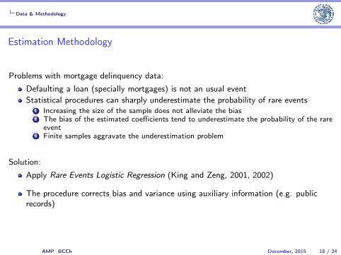
Problems with mortgage delinquency data:

Defaulting a loan (specially mortgages) is not an usual eventStatistical procedures can sharply underestimate the probability of rare events

1 Increasing the size of the sample does not alleviate the bias2 The bias of the estimated coefficients tend to underestimate the probability of the rare

event3 Finite samples aggravate the underestimation problem

Solution:

Apply Rare Events Logistic Regression (King and Zeng, 2001, 2002)

The procedure corrects bias and variance using auxiliary information (e.g. publicrecords)


Results

Estimation Results 1: No interactions

Dep. Var.: Mortgage Default Dummy Model 1 Model 2 Model 3 Model 4Idiosyncratic - Demographic VariablesNumber of persons in house 0.211*** 0.235*** 0.214** 0.213**

(0.0715) (0.0826) (0.0844) (0.0856)Income (in logs) -0.827*** -0.563*** -0.734*** -0.524***

(0.133) (0.153) (0.155) (0.162)Primary Education 0.348 0.0446 0.215 0.109

(0.333) (0.424) (0.440) (0.466)Tertiary Education -0.633*** -0.417 -0.554* -0.397

(0.241) (0.291) (0.308) (0.309)Gender -0.285 -0.214 -0.285 -0.301

(0.199) (0.229) (0.244) (0.242)Age 18-35 -0.0218 -0.155 0.0266 0.105

(0.260) (0.295) (0.306) (0.308)Age 55-99 -0.699 -0.0802 -0.0578 -0.0759

(0.603) (0.675) (0.696) (0.683)Idiosyncratic - Finance Variables

Negative Shock 1.745*** 1.715*** 1.668*** 1.683***(0.207) (0.245) (0.255) (0.256)


Renegotiation 1.352*** 1.052*** 1.016*** 1.073***(0.244) (0.309) (0.332) (0.336)


Results

Estimation Results 1: No interactions

Dep. Var.: Mortgage Default Dummy Model 1 Model 2 Model 3 Model 4Idiosyncratic - Finance Variables

Negative Shock 1.745*** 1.715*** 1.668*** 1.683***(0.207) (0.245) (0.255) (0.256)


Renegotiation 1.352*** 1.052*** 1.016*** 1.073***(0.244) (0.309) (0.332) (0.336)

Systemic VariablesCurrent Loan to Value 0.253**

(0.117)Initial House Price (in logs) -0.416*** -0.450***

(0.113) (0.152)Initial Loan to Value 0.0407 -0.0835

(0.0249) (0.0794)Constant 6.125*** 9.095*** 4.663** 9.413***

(1.761) (2.302) (2.074) (2.631)Observations 1,894 1,446 1,301 1,337

Note: Robust standard errors in parentheses. Significance: *** p<0.01, ** p<0.05, * p<0.1


Results

Estimation Results 2: Including Interactions

Dep. Var.: Mortgage Default Dummy Model 1 Model 2Idiosyncratic - Demographic VariablesNumber of persons in house 0.237*** 0.231***

(0.0820) (0.0819)Income (in logs) -0.578*** -0.582***

(0.150) (0.149)Primary Education 0.0564 0.0804

(0.421) (0.414)Tertiary Education -0.423 -0.425

(0.290) (0.290)Gender -0.260 -0.247

(0.228) (0.227)Age 18-35 -0.189 -0.195

(0.298) (0.298)Age 55-99 -0.0714 -0.0950

(0.675) (0.675)


Results

Estimation Results 2: Including Interactions

Dep. Var.: Mortgage Default Dummy Model 1 Model 2Idiosyncratic - Finance Variables

Negative Shock 1.678***(0.245)

Credit Applications Rejected 0.687 0.677(0.437) (0.439)

Renegotiation 1.319*** 1.325***(0.277) (0.276)

Systemic VariablesInitial House Price (in logs) -0.417*** -0.443***

(0.112) (0.111)Interaction Variables

Income and current loan to value 0.0199** 0.0195**(0.00810) (0.00814)

Initial House Price and Negative shock 0.102***(0.0147)

Constant 9.326*** 9.817***(2.265) (2.243)

Observations 1,446 1,446

Note: Robust standard errors in parentheses. Significance: *** p<0.01, ** p<0.05, * p<0.1


Final remarks

Final remarksWe are able to estimate a micro-powered model of mortgage default determinantsContrary to the existing literature, we find that interaction between macro and microfactors is key

Income is an important determinant of the probability of defaultA negative shock in the recent past significantly increases the probability ofdefaulting a mortgage loanHigher housing prices lessen the probability of default (the contrary is problematic)

A higher value of the interaction between income and current LTV is associated tohigher mortgage defaultAlso, a higher value of the interaction between origination housing prices andnegative budget shocks is associated with higher default rates

We propose to extend this framework to analyze further financial issues in a moregeneral setting


Appendix

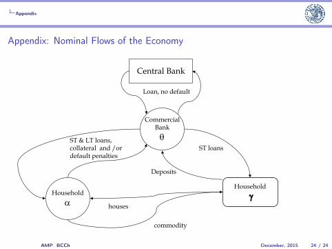
Appendix: Nominal Flows of the Economy

Household

Commercial Bank

Central Bank

ST & LT loans, collateral and /or default penalties

Loan, no default

Household

houses

Deposits

commodity

ST loans


Documents

A micro-powered model of mortgage default risk for full … · · 2016-04-25A micro-powered model of mortgage default risk for full recourse economies, with an application to the