Embed Size (px)
Citation preview

A Methodology for identifying and improving occupant
behavior in residential buildings
Zhun (Jerry) Yu1, Fariborz Haghighat
1, Benjamin C. M. Fung
2, Edward Morofsky
3,
Hiroshi Yoshino4
1Department of Building, Civil and Environmental Engineering, Concordia University,
Montreal, Quebec, H3G 1M8, Canada 2Concordia Institute for Information Systems Engineering, Concordia University,
Montreal, Quebec, H3G 1M8, Canada 3Real Property Branch, Public Works and Government Services Canada, Place du Portage III,
8B1, Gatineau, Québec, K1A 0S5 Canada 4Department of Architecture and Building Science, Tohoku University, Japan
Abstract
This paper reports the development of a methodology for identifying and improving
occupant behavior in existing residential buildings. In this study, end-use loads were
divided into two levels (i.e. main and sub-category), and they were used to deduce
corresponding two-level user activities (i.e. general and specific occupant behavior)
indirectly. The proposed method is based on three basic data mining techniques:
cluster analysis, classification analysis, and association rules mining. Cluster analysis
and classification analysis are combined to analyze the main end-use loads, so as to
identify energy-inefficient general occupant behavior. Then, association rules are
mined to examine end-use loads at both levels, so as to identify energy-inefficient
specific occupant behavior. In order to demonstrate its applicability, this methodology
was applied to a group of residential buildings in Japan, and one building with the
most comprehensive household appliances was selected as the case building. The
results show that, for the case building, the method was able to identify the behavior
which needs to be modified, and provide occupants with feasible recommendations so
that they can make required decisions. Also, a reference building can be identified for
the case building to evaluate its energy-saving potential due to occupant behavior
modification. The results obtained could help building occupants to modify their
behavior, thereby significantly reducing building energy consumption. Moreover,
given that the proposed method is partly based on the comparison with similar
buildings, it could motivate building occupants to modify their behavior.
Keywords: Occupant behavior; Building energy consumption; Data mining;
Evaluation; Identification

Nomenclature
SHW Supply hot water load
LIGHT Lighting load
KITCH Kitchen load
REFRI Refrigeration load
E&I Entertainment & Information load
H&S Housework & Sanitary load
OTHER Others load
T Outdoor temperature (annual average) (°C)
RH Outdoor relative humidity (annual average)
V Outdoor air velocity (annual average) (m/s)
RA Outdoor solar radiation (annual average) (MJ/m2)
NO Number of occupants
FA Floor area (m2)
HLC Heat loss coefficient (W/m2K)
ELA Equivalent leakage area (cm2/m
2)
CO Construction
SH Space heating
WH Water heating
KIT Kitchen
HT House type

1. Introduction
Currently, residential sector building energy consumption forms a large part of the
total national energy consumption (TNEC) in both developed and developing
countries. For example, in the US and Japan, residential building energy consumption
accounts for 25% and 26% of TNEC, respectively [1]. In China and Thailand, the
proportion of residential building energy consumption to TNEC is 11.3% and 15.4%,
respectively [2-3]. Furthermore, with the rapid growth of the economy and rising
living standards, there is a rapid increase in energy consumption in the residential
sector worldwide [4-6]. The high energy demand in residential buildings, which is
also growing rapidly, necessitates a better understanding of its major influence factors.
At the same time, it is necessary to develop a methodology for reducing energy
consumption. For instance, to combat this rapid increase in energy use some utility
companies and government organizations provide building owners with a “booklet”
which gives tips on reducing the building energy consumption. These tips are general
in nature and are not specific.
Among various factors influencing residential building energy consumption, occupant
behavior plays an essential role and is difficult to investigate analytically due to its
complicated characteristics [7]. Note that here occupant behavior refers to activities
that have a direct or indirect impact upon building energy consumption. For example,
occupants turn on/off lights, TV sets, computers, microwave ovens, and so on.
Commonly such behavior is associated with various household appliances and thus
can be deduced indirectly from corresponding end-use loads. For example, the total
daily (or monthly, annual) lighting energy consumption in a residential building
qualitatively indicates the duration of lighting usage in this day (or month, year).
Accordingly, any improvement in the occupant behavior leads to the reduction of the
residential building energy consumption.
Recently, there has been increasing interest in studying occupant behavior and
developing a methodology for identifying the corresponding energy-saving potential.
Ouyang and Hokao [8] investigated the energy-saving potential by improving user
behavior in 124 households in China. In this study, these houses were divided into two
groups: one group received an energy-saving education and was encouraged to put
energy-conscious behavior into effect, while the other group was required to keep
behavior intact. Comparisons were made between monthly household electricity uses
in July 2007 and July 2008 for both groups. It was found that, on average, effective
promotion of energy-conscious behavior could reduce household electricity
consumption by more than 10%. Al-Mumin et al. [9] simulated occupant behavior
improvement (i.e. simulation of occupant behaviour before and after modification)
and corresponding annual electricity consumption reduction by using the energy
simulation program ENERWIN. They first collected data and information on
occupancy patterns and operation schedules of electrical appliances in 30 selected
residences in Kuwait. This data and information were then used in ENERWIN to

replace the default value. A house then was selected as a case study and the simulation
results showed that the annual electricity consumption in this house was increased by
21%. The results also indicated that the ENERWIN’s default parameters (i.e.
parameters taken from the software manual) are probably more appropriate for the
Western living lifestyle. Moreover, it was found that a reduction of energy
consumption by 39% can be achieved by improving occupant behavior such as
turning off the lights when rooms were empty and setting the air conditioner
thermostat to a higher temperature (but still within the comfort level).
Basically, two approaches (i.e., energy-saving education and building simulation),
were used to improve building occupant behavior and identify the corresponding
energy-saving potential. These two approaches can help to modify occupant behavior
and have an immediate effect on building energy consumption reduction. However,
both of the approaches have certain limitations. With regard to the energy-saving
education approach, commonly detailed energy-saving measures and tips on efficient
use of various household appliances should be provided for occupants. Considering
that a family normally has a number of appliances and that each appliance may have
various tips (e.g. for the usage of refrigerators, various tips can be given: reduce door
open times, keep its coils and filters clean, keep it far from other heat sources,etc),
there could be a large number of energy-saving measures and tips for an individual
family. For example, one family may have 30 household appliances, with each
appliance having an average of 8 energy-saving tips. Accordingly, the occupants need
to understand and remember 240 tips, which may be quite impractical. Although a
booklet of these tips can be prepared for building occupants, it is very difficult for
occupants to remember distinctly all these tips and implement them for a long time in
practice. Furthermore, occupants may not fully understand and have confidence in
these tips’ effects as they only provide qualitative information. In addition, some
energy-saving opportunities can only be initiated by building occupants. For example,
when occupants realize they have consumed too much energy on both computers and
TVs, they can avoid using both devices simultaneously when they can only focus on
one of them, or make a conscious effort to reduce usage time.. Therefore, instead of
simply providing occupants with a number of general energy-saving
recommendations, it is more rational and efficient to help them modify the behaviour
in two steps. First, it is necessary to identify the behaviour that needs to be modified.
This can be achieved by analyzing measured data. Second, feasible recommendations
to improve the identified behaviour can be presented with the goal of reducing energy
consumption in the home. With regard to the building simulation approach, current
simulation tools can only imitate some typical activities such as the control of
sun-shading devices in a rigid way, while realistic building occupant behavior patterns
are more complicated.
This paper reports the development of a rational methodology for identifying and
improving occupant behavior in existing residential buildings, based on an analysis of
collected data and information. In particular, feasible recommendations are made for

assisting occupants to modify their behaviour so as to reduce energy consumption.
2. Methodology
A new methodology is proposed for efficiently improving occupant behavior in
existing residential buildings, and evaluating the energy-saving potential resulting
from these modifications. As mentioned previously, end-use loads are used to deduce
user activities indirectly. Specifically, these loads are used to map onto occupant
behavior at two levels, as shown in Fig. 1.
End-use loads in residential buildings
Level 1
Main end-use loads
1) water heater...
2) lamp, table lamp...
3) rice cooker, dishwasher...
4) refrigerator
5) television, computer...
6) washing machine, dryer...
7) unclear items
1) Hot water supply
2) Lighting
3) Kitchen
4) Refrigerator
5) Entertainment & Information
6) Housework & Sanitary
7) Others
Level 2
Sub-category end-use loads
General occupant behavior Specific occupant behavior
Fig.1. Two-level end-use loads
Level 1 loads are divided into seven main end-use loads), , each of which can be
further divided into various end-users in level 2. The seven end-use loads in level 1
are assumed to be non-weather-dependent [10], due to the fact that the usage of these
appliances (i.e. lighting, refrigerators, etc.) is mainly determined by occupants’
presence and their behaviour, though it may also be partly impacted by weather
conditions. At the same time, given that HVAC loads in the investigated buildings are
primarily determined by weather conditions (especially outdoor air temperature), the
HVAC load is not taken into consideration in this study though it may also partly be
impacted by occupant behaviour. It should be mentioned that, the level 2 end-users
are not fixed in different residential buildings since commonly different families have
different household appliances. The level 1 and level 2 loads are mapped onto general
occupant behavior, such as activities associating with lighting and hot water supply,
and specific occupant behavior, such as the use of computers and washing machines.

For demonstration purposes, a group of buildings is used to show the practical
application of this methodology. Recommendations for improving occupant behaviour
are provided for a selected building (case building) within this group.
The methodology is briefly described as follows.
(1) Identify energy-inefficient general occupant behavior in the case building.
(2) Identify a reference building for the case building to evaluate its energy-saving
potential, and further determine its energy-inefficient general occupant behavior
by comparison with the reference building.
(3) Identify energy-inefficient specific occupant behavior in the case building.
The proposed methodology can be demonstrated in a five-step process, as shown in
Fig. 2.
Provide recommendations for modifying occupant behavior for the
case building occupants
Case building
(data measurement)
Database development
(related buildings)
Clustering-then-classification
Reference building identification
for the case building
Association rule mining in the case building
Fig.2. Methodology of evaluating and efficiently improving occupant behavior in the
case building
Each step in this methodology is briefly explained as follows:
(1) First, a database should be developed based on the collection of measured data for
the case building and other related buildings (e.g. buildings selected in the same city
or country). The daily (or hourly) level 2 end-use loads should be measured, and the
level 1 end-use loads can be accumulated based on the level 2 data. The database

should also contain information about building-related parameters, such as floor area
and number of occupants.
(2) Through clustering analysis, all the related buildings in the database are clustered
into different groups in terms of the level 1 loads (for each main end-use load, the
annual per capita end-use loads is used for comparison). Accordingly, general
occupant behavior in different buildings in the same group has a high similarity, but is
quite different from that in other groups. Specifically, comparing with occupants in
other clusters, on average each occupant in the same cluster consumes similar
amounts of energy each year in terms of the seven level 1 end-use loads. Note that
these seven loads are taken into consideration separately but simultaneously.
Consequently, by comparing with other clusters, the characteristics of occupant
behavior in each cluster can be identified. Such information can help building
occupants to evaluate their own behavior among all the building owners in the
database, thereby identifying general occupant behaviour which results in inefficient
use of energy. Then, data classification based on the generated clusters is performed,
and specifically, a decision tree [11] is developed. By using the generated decision
tree, a building can be assigned to a specific cluster, provided its level 1 loads are
available. In particular, once the case building has been assigned to a cluster, its
general energy-inefficient occupant behaviour can be determined. It should be
mentioned that, the decision tree was selected and used in this study due to the fact it
can provide useful information which can help to understand the role of building
occupant behavior in improving energy saving [12].
(3) Among the related buildings in the database, a reference building (RB) is
identified for the case building to evaluate its energy-saving potential due to the
occupant behavior modification. The RB is selected from the same cluster as the case
building so that both of them have similar holistic occupant behavior patterns. The
comparison with the RB also shows the case building occupants which general
occupant behavior still need to be modified.
(4) After identifying the energy-inefficient general occupant behavior through
clustering analysis and RB identification, it is necessary for the case building owner
to know which specific activities and corresponding appliances deserve extra attention.
Therefore, association rules are mined to identify the associations and correlations
between various user activities in the case building, in order to highlight
energy-saving opportunities.
(5) Recommendations for energy-efficient activities are provided for the case building
occupants, so that they can modify their behavior.
In the following section, various data mining techniques employed in this
methodology are first introduced. Then the steps in identifying a RB for the case
building are explained.

2.1. Clustering-then-classification
2.1.1. Cluster analysis
Cluster analysis is the process of grouping data objects into clusters so that objects in
the same cluster have high similarity, while objects in different clusters have low
similarity. Fig. 3 shows a clustering schema based on a hypothetical residential
building data table. It contains various end-use loads such as supply hot water and
lighting.
Attribute 1
(supply hot water)
Unit: MJ per capita per year
...Attribute m
(lighting)
Unit: MJ per capita per yearInstance 1
…
Instance i
Instance j
...
Instance n
x ... x
... ... ...
x ... x
x ... x
... ... ...
x ... x
Cluster 1
Cluster w
... ... ... ...
Instance
...
Fig.3. Clustering schema
This table consists of m attributes and n instances. Each attribute represents a variable
and each instance denotes a building. All the instances are grouped into w clusters.
Accordingly, these w clusters are homogeneous internally and heterogeneous between
different clusters [11]. Such internal cohesion and external separation are based upon
the various end-use loads, which can be mapped onto corresponding building
occupant behavior. It implies that buildings in the same cluster have similar holistic
occupant behavior patterns; while the patterns are significantly distinct for the
buildings in different clusters.
The dissimilarity between data objects in the database is calculated using the distance
between them in the cluster analysis. In this study, the most popular distance measure,
Euclidean distance, was used [11]:
𝑑(𝑘, 𝑙) = √(𝑥𝑘1 − 𝑥𝑙1)2 + (𝑥𝑘2 − 𝑥𝑙2)2 + ⋯ + (𝑥𝑘𝑛 − 𝑥𝑙𝑛)2
where k = (xk1, xk2, …, xkn) and l = (xl1, xl2, …, xln) are buildings. xk1, …, xkn are n
parameters of k and xl1, …, xln are n parameters of l.
Commonly used clustering algorithms include K-means, K-medoids, and CLARANS
[11]. In this study, we employ the K-means, along with the open-source data mining
program RapidMiner [13], to perform cluster analysis due to its efficiency and wide

applicability.
The K-means algorithm is one of the simplest partition methods to solve clustering
problems. Given a dataset (D) containing w objects, the K-means algorithm aims to
partition these w objects into k clusters with two restraints: 1) the center of each
cluster is the mean position of all objects in that cluster, 2) each object is assigned to
the cluster with the closest center. The algorithm consists of five steps: 1) Randomly
select k observations from D as the initial cluster centers, 2) Calculate the distance
between each remaining observations and each initially chosen center, 3) Assign each
remaining observation to the cluster with the closest center, 4) Recalculate the mean
values, i.e., the cluster centers, of the new clusters, and 5) Repeat Steps 2 to 4 until the
algorithm converges, meaning that the cluster centers do not change.
In RapidMiner, the performance of clustering algorithms is evaluated by using the
Davies Bouldin index (DBI) [14]. This index is defined as the ratio of the sum of
average distance inside clusters to distance between clusters.
𝐷𝐵𝐼 =1
𝑛∑ 𝑚𝑎𝑥
𝑖≠𝑗[𝑅𝑖 + 𝑅𝑗
𝑀𝑖,𝑗]
𝑛
𝑖=1
where
n: number of clusters,
Ri, Rj: average distance inside cluster i and cluster j by averaging the distance between
each cluster object and the cluster center,
Mi,j: distance between cluster centers.
DBI is small if each cluster is comparatively dense; while different clusters are far
from each other. Consequently, a smaller DBI indicates better performance of the
clustering algorithm. It should be mentioned that the K-means is quite sensitive to
initial cluster centers. Therefore, different values should be tried so as to obtain the
minimum DBI. At the same time, the number of clusters should be specified in
advance.
2.1.2. Classification analysis
Among various classification algorithms, decision tree was selected and used in this
study. The decision tree methodology is one of the most commonly used data mining
methods [11, 15]. It uses a flowchart-like tree structure to segregate a set of data into
various predefined classes, thereby providing the description, categorization, and
generalization of given datasets. As a logical model, decision tree shows how the
value of a target variable can be predicted by using the values of a set of predictor
variables.

Root node
Outdoor air temperature ≤ - 6 °C ?
Leaf node
SHW is HIGH
(60)
Internal node
Empty room ?
Yes No
Yes No
Leaf node
SHW is LOW
(10)
Leaf node
SHW is HIGH
(30)
Fig.4. Schematic illustration of a simple hypothetical decision tree
Fig. 4 gives a simple decision tree indicating whether the supply hot water load (SHW)
in a residential building is high or low in winter. For this example, assume 100 data
records are used to build this decision tree, and that each record has three attributes:
outdoor air temperature, occupant presence, and the level of SHW.
The target variable for the above decision tree is the level of SHW, with potential
states being classified as either HIGH or LOW. The predictor variables are outdoor air
temperature (≤ - 6°C or > - 6°C) and occupant presence (empty or occupied). As
shown in Fig. 4, the decision tree consists of three kinds of nodes: root node, internal
node, and leaf node. Root nodes and internal nodes denote a binary split test on an
attribute while leaf nodes represent an outcome of the classification (i.e. a categorical
target label). By using this decision tree, the SHW level classification (‘i.e HIGH or
LOW) can be predicted. For example, if the outdoor air temperature is higher than -
6 °C and the room is empty, SHW is LOW; otherwise it is HIGH.
Decision tree generation is in general a two-step process, namely learning and
classification, as shown in Fig. 5. In the learning process, the collected data is split
into two subsets: a training set and a testing set. Creation of training sets and testing
sets is an important part of evaluating data mining models. Usually, most of the data
records in the database are arbitrarily selected for training and the remaining data
records are used for testing. Note that training sets and testing sets should come from
the same population but should be disjoint. Then, a decision tree generation algorithm
takes the training data as an input, with the corresponding output being a decision tree.
Commonly used decision tree generation algorithms include ID3 [15], classification
and regression trees (CART) [16], and C4.5 [17]. In this study, we employ C4.5, along
with the open-source data mining software RapidMiner [13], to build a decision tree.
This software is selected due to its flexibility and wide applicability to different types
of data. In the classification process, the accuracy of the obtained decision tree is first
evaluated by making predictions against test data. The accuracy of a decision tree is
measured by comparing the predicted target values with the true target values of the
test data. If the accuracy is considered acceptable, the decision tree can be applied to
new datasets for classification and prediction; otherwise, the reason for any

inaccuracies should be identified and corresponding solutions should be adopted to
address these problems.
Accuracy is considered acceptable ?
Analyzing training data by a decision tree
algorithm and generating decision tree
Estimating the accuracy of obtained
decision tree using test data
Splitting dataset into
training data and test data
Applying decision tree to future data
Y
NIdentifying reasons
and finding solutions
Learning
Classfication
Fig.5. Procedure of decision tree generation
The procedure of generating a decision tree from the training data is as follows.
Initially, all records in the training data are grouped together into a single partition. At
each iteration, the algorithm chooses a predictor attribute that can “best” separate the
target class values in the partition. The ability of a predictor attribute to separate the
target class values is measured based on an attribute selection criterion, which was
introduced in [12]. After a predictor attribute is chosen, the algorithm splits the
partition into child partitions such that each child partition contains the same value of
the chosen selected attribute. The decision tree algorithm iteratively splits a partition
and stops when any one of the following terminating conditions is met:
All records in a partition share the same target class value. Thus, the class
label of the leaf node is the target class value.
There are no remaining predictor attributes that can be used to further split a
partition. In this case, the majority target class values become the label of the
leaf node.
There are no more records for a particular value of a predictor variable. In this
case, a leaf node is created with the majority class value in the parent partition.
2.1.3. Reference Building (RB) identification
RB is normally utilized as a benchmark for comparison and the method of defining a

RB depends on the purpose of study. In this study, the RB was defined to evaluate the
energy-saving potential due to occupant behavior modification in the case building,
and identify occupant behavior needing to be improved. Therefore, the definition of
RB for the case building should comply with the following two rules:
Rule 1: The holistic occupant behavior patterns in RB and the case building should be
as similar as possible. Different residential building occupants normally have different
lifestyles and behavior patterns. In general, it is very difficult for building occupants
to make dramatic lifestyle changes in order to reduce energy consumption. Hence,
among the related buildings in the database, buildings with more similar occupant
behavior patterns should be considered when evaluating the energy-saving potential
for the case building. This implies that potential RB candidates should be chosen from
buildings in the same cluster as the case building, since occupant behavior in the same
cluster has a high similarity in comparison to one another, but is quite dissimilar to
that in the other clusters.
Rule 2: Among all the potential RB candidates, the selected RB should have the
highest similarity to the case building in terms of building-related parameters, such as
outdoor temperature and floor area. This can also improve the reliability of
comparative results between the two buildings. Euclidean distance can be used to
define the similarity.
With consideration of the two rules, RB identification for the case building consists of
the following steps:
Step 1: Assign the ‘case building’ to a cluster according to the level 1 loads and the
generated decision tree;
Step 2: calculate the total energy consumption (i.e. the sum of the seven main end-use
loads) in the case building and other buildings in the same cluster. Rank the total
energy consumption in all these buildings;
Step 3: Identify the RB. Buildings in the same cluster with lower total energy
consumption than the case building are used as potential RB candidates. Then, based
on building-related parameters and Euclidean distance, the most similar building to
the case building among the candidates can be found. This building is identified as
RB for the case building.
2.1.4 Association rule mining
In data mining, association rules are often used to represent patterns of parameters
that are frequently associated together. An example is given to illustrate the concept of
association rules. Assume that 100 occupants live in 100 different rooms in the same
building and each room has both a window and a door. Moreover, 40 occupants open
the windows and 20 occupants open the doors. If 10 occupants open both the
windows and doors simultaneously, it can be calculated that these 10 occupants
account for 10% of all the building occupants (10/100 = 10%), and 25% of the

occupants who open windows (10/40 = 25%). Then, the information that occupants
who open windows also tend to open doors at the same time can be represented in the
following association rule:
open_windows → open_doors [𝑠𝑢𝑝𝑝𝑜𝑟𝑡 = 10%, 𝑐𝑜𝑛𝑓𝑖𝑑𝑒𝑛𝑐𝑒 = 25%]
In this statement, support and confidence are employed to indicate the validity and
certainty of this association rule. Different users or domain experts can set different
thresholds for support and confidence according to their own requirements, in order to
discover useful knowledge eventually. Accordingly, the association rule mining
(ARM) can be defined as finding out association rules that satisfy the predefined
minimum support and confidence from a given database.
Mathematically, support and confidence can be calculated by probability, P(X∪Y),
and conditional probability, P(Y|X), respectively (X denotes the premise and Y
denotes the consequence in the sequence). That is,
𝑠𝑢𝑝𝑝𝑜𝑟𝑡(X → Y) = P(X ∪ Y)
𝑐𝑜𝑛𝑓𝑖𝑑𝑒𝑛𝑐𝑒(X → Y) = P(Y|X)
Another concept, lift, which is similar to confidence, is commonly used to
demonstrate the correlation between the occurrence of X and Y when conducting the
ARM. Mathematically,
𝑙𝑖𝑓𝑡(X → Y) =P(X ∪ Y)
P(X)P(Y)=
P(Y|X)
P(Y)
Particularly, a lift value greater than 1 represents a positive correlation (the higher this
value is, the more likely that X coexists with Y, and there is a certain relationship
between X and Y [18]) while a lift value less than 1 represents a negative correlation.
If the value is equal to 1, i.e. P(X ∪ Y) = P(X)P(Y) , the occurrence of X is
independent of the occurrence of Y, and there is no correlation between X and Y.
Commonly used ARM algorithms include the Apriori algorithm and the
frequent-pattern growth (FP-growth) algorithm [11]. In this study, we employ the
FP-growth algorithm, along with the open-source data mining software RapidMiner
[13], to mine association rules due to its high efficiency and wide applicability. For
the specific algorithm of FP-growth the reader can refer to [11].
Additionally, in order to perform the ARM, the value of quantitative attributes
generally needs to be classified into categorical values. Considering that most
attributes used in the ARM in this study are end-use electricity loads, a two-interval
scale (i.e., HIGH and LOW) was applied to represent high and low energy

consumption. Such high and low energy consumption can then be qualitatively
mapped onto energy-inefficient and energy-efficient occupant behavior. It should be
mentioned that HIGH and LOW quite possibly, but do not necessarily, correspond to
energy-inefficient and energy-efficient occupant behaviour in practice. For example,
less energy efficient appliances will also cause higher energy consumption. However,
given that energy-inefficient behaviour will waste energy and normally cause high
energy consumption, such mapping was still used in this study. Consequently, the
results need to be carefully analyzed and energy-inefficient behaviour should be
eventually identified based on practical occupant behaviour patterns. Specifically, for
each quantitative attribute, data ranged from the average of the maximum and
minimum to the maximum value is ‘HIGH’, and data ranged from the minimum value
to the average of the maximum and minimum is ‘LOW’.
3. Data collection and pre-processing
3.1. Data collection
To evaluate and improve the energy performance of residential buildings, a project
entitled “Investigation on Energy Consumption of Residents All over Japan” was
carried out by the Architecture Institute of Japan from December 2002 to November
2004 [19]. For this project, field surveys on energy-related data and other relevant
information were carried out in 80 residential buildings located in six different
districts in Japan: Hokkaido, Tohoku, Hokuriku, Kanto, Kansai, and Kyushu. Table 1
shows the survey items and corresponding investigation methods. Fig. 6 shows the
measuring instruments which were used to monitor temperature and consumptions of
electricity, gas, and/or kerosene. As mentioned previously, the collected data can be
divided into two levels. However, for the level 2 data, currently only daily data is
available (instead of data at 1 or 5 minute time steps).
Table 1
Investigation items and methods
Method Survey items Measuring time
Field
measurement
Different end-use loads of all
kinds of fuel
Electricity Measured every minute
Gas Measured every 5 minutes
Kerosene Measured every 5 minutes
Indoor air temperature (1.1m above floor) Measured every 15 minutes
Questionnaire
survey
Lifestyle, Utilization of equipment, Annual
income, etc. Once only
Inquiring survey Other issues, such as basic building information Once only

Fig.6. Measuring instruments (from left to right: electricity, gas, kerosene and air
temperature)
3.2. Data pre-processing
3.2.1. Data integration and reduction
Scrutinizing the data from the 80 buildings, it was found that only 67 sets were
complete, while 13 sets had missing values of energy consumption data. Data
integration was carried out for the detection and resolution of data value conflicts. For
example, diverse energy units of different kinds of primary energy sources used by
the various buildings (including electricity, natural gas, and kerosene) were converted
to MJ based on conversion coefficients in Table 2. After conversion, they could be
added directly. Then, data reduction was performed to obtain a smaller representation
of the original data. For example, readings of each main end-use load at different
intervals (e.g., 1 or 5 minutes) were averaged over one year. The resulting data was
stored in a database.
Table 2
Conversion coefficients of different fuels
Fuel Conversion coefficient Unit
Electricity 3.6 MJ/kWh
City gas (4A-7C) 20.4 MJ/Nm3
City gas (12A-13C) 45.9 MJ/Nm3
Liquefied petroleum gas (LPG) 50.2 MJ/Nm3
Kerosene 36.7 MJ/L
3.2.2 Case building selection
As mentioned earlier, for demonstration purposes, one building with the most
comprehensive household appliances should be selected as the case building, and the
remaining 66 buildings are used for both clustering-then-classification and RB
identification. Data inspection indicates that a building located in Hokkaido has the
most appliances, as shown in Table 3. Table 3 also shows some measured
environmental parameters of this building such as indoor air temperature and
humidity. These parameters will also be used in the ARM to analyze the associations
between them and occupant behaviour.
Table 3
Appliances in the case building and environmental parameters used in ARM
No. Appliances/ No. Appliances/ No. Appliances/
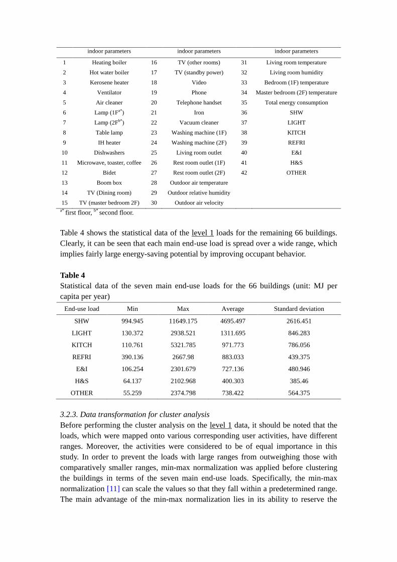
indoor parameters indoor parameters indoor parameters
1 Heating boiler 16 TV (other rooms) 31 Living room temperature
2 Hot water boiler 17 TV (standby power) 32 Living room humidity
3 Kerosene heater 18 Video 33 Bedroom (1F) temperature
4 Ventilator 19 Phone 34 Master bedroom (2F) temperature
5 Air cleaner 20 Telephone handset 35 Total energy consumption
6 Lamp (1Fa*) 21 Iron 36 SHW
7 Lamp (2Fb*) 22 Vacuum cleaner 37 LIGHT
8 Table lamp 23 Washing machine (1F) 38 KITCH
9 IH heater 24 Washing machine (2F) 39 REFRI
10 Dishwashers 25 Living room outlet 40 E&I
11 Microwave, toaster, coffee 26 Rest room outlet (1F) 41 H&S
12 Bidet 27 Rest room outlet (2F) 42 OTHER
13 Boom box 28 Outdoor air temperature
14 TV (Dining room) 29 Outdoor relative humidity
15 TV (master bedroom 2F) 30 Outdoor air velocity
a* first floor,
b* second floor.
Table 4 shows the statistical data of the level 1 loads for the remaining 66 buildings.
Clearly, it can be seen that each main end-use load is spread over a wide range, which
implies fairly large energy-saving potential by improving occupant behavior.
Table 4
Statistical data of the seven main end-use loads for the 66 buildings (unit: MJ per
capita per year)
End-use load Min Max Average Standard deviation
SHW 994.945 11649.175 4695.497 2616.451
LIGHT 130.372 2938.521 1311.695 846.283
KITCH 110.761 5321.785 971.773 786.056
REFRI 390.136 2667.98 883.033 439.375
E&I 106.254 2301.679 727.136 480.946
H&S 64.137 2102.968 400.303 385.46
OTHER 55.259 2374.798 738.422 564.375
3.2.3. Data transformation for cluster analysis
Before performing the cluster analysis on the level 1 data, it should be noted that the
loads, which were mapped onto various corresponding user activities, have different
ranges. Moreover, the activities were considered to be of equal importance in this
study. In order to prevent the loads with large ranges from outweighing those with
comparatively smaller ranges, min-max normalization was applied before clustering
the buildings in terms of the seven main end-use loads. Specifically, the min-max
normalization [11] can scale the values so that they fall within a predetermined range.
The main advantage of the min-max normalization lies in its ability to reserve the

relationships between the initial data, since it carries out a linear normalization.
Assume that xmax and xmin are the original maximum and minimum values of a
numerical attribute (i.e. the level_1 end-use loads in this study). By using the
min-max normalization, a value of this attribute (e.g. x) can be transformed to x’ in
the new specified range [x’min, x’max] by calculating
𝑥′ =𝑥 − 𝑥𝑚𝑖𝑛
𝑥𝑚𝑎𝑥 − 𝑥𝑚𝑖𝑛(𝑥′
𝑚𝑎𝑥− 𝑥′
𝑚𝑖𝑛) + 𝑥′𝑚𝑖𝑛
In this study, the new range is defined as [0, 1]. Table 5 shows the statistical data of
the level 1 loads for the remaining 66 buildings after min-max normalization.
Table 5
Statistical data after normalization
End-use load Min Max Average Standard deviation
SHW 0 1 0.347 0.246
LIGHT 0 1 0.421 0.301
KITCH 0 1 0.165 0.151
REFRI 0 1 0.216 0.193
E&I 0 1 0.283 0.219
H&S 0 1 0.165 0.189
OTHER 0 1 0.295 0.243
3.2.4. Removal of outliers for conducting ARM in the case building
Outliers are data objects whose values are grossly different (i.e. much higher or lower)
from others in the database. Outliers regularly occur in building energy
consumption measurement. They are often indicative of measurement errors, and thus
must be removed. Removal of outliers plays a crucial role in preparing for the ARM,
since outliers produce a large measure of skewness and have a significant influence on
the partition of attribute values into different intervals. For example, suppose an
attribute ranges from 0 to 10, and can be discretized into two intervals, [0, 5) and [5,
10] (or LOW and HIGH), by using the methods mentioned previously. If there exists
an outlier (e.g. 30), then the two intervals are [0, 15) and [15, 30] (or LOW and HIGH)
by using the same method. Accordingly, all the data are defined as LOW except the
outlier, which is not actually true.
Various methods can be used for effective detection and removal of outliers. In this
study, a method based on the lower quartile (Q1) and the upper quartile (Q3) of the
standard boxplot was used due to its simplicity [20]. Specifically, outlying values can
be distinguished using the following two rules:
Rule 1: data values that are less than Q1 – 1.5 × (Q3 – Q1) are defined as outliers
Rule 2: data values that are larger than Q3 + 1.5 × (Q3 – Q1) are defined as outliers
With consideration of the seasonality of occupant behavior, the ARM was performed

based on seasonal data instead of annual data in this study for demonstration purposes.
Given that the case building is located in Hokkaido, the coldest area in Japan, the
winter data in 2003 was mined to generate association rules. Fig. 7 shows the
distribution of two intervals of all the ARM attributes after the removal of outliers.
Note that the numbers in the abscissa represent the ARM attributes, and correspond to
the number in Table 3. Clearly, it can be observed that most of the percentages range
from 30% to 70%, indicating a roughly uniform distribution.
Fig.7. Distribution of two intervals of all ARM attributes after the removal of outliers
4. Results and discussion
4.1. Clustering-then-classification
4.1.1. Clustering results
After data pre-processing, the cluster analysis was conducted for the 66 buildings
using the RapidMiner. With consideration of the size of the database, four clusters
were determined by the K-means algorithm and the performance vector (Davies
Bouldin index, DBI). The results of the cluster analysis are given in Table 6. Cluster
centroid, which represent the mean value for each dimension, were used to
characterize building occupant behavior in the four clusters. For example, in
comparison with building occupant behavior in the other clusters, user activities in
cluster_2 caused medium energy consumption in supply hot water (the cluster
centroid of SHW in this cluster is 0.440, which is of medium value among the four
clusters), high energy consumption in lighting, medium energy consumption in
kitchen, etc. Moreover, cluster_2 has significantly higher energy consumption for
lighting; this indicates that, in general, building owners in cluster_2 should give
primary consideration to the activities related to lighting in order to save energy.
Similarly, other clusters can be explained. It should be noted that nearly half of the
data records (44%) were grouped into cluster_1, which represents low energy
consumption in most of the main end-use loads. A possible explanation for this is that
0%
10%
20%
30%
40%
50%
60%
70%
80%
90%
100%
1 4 7 10 13 16 19 22 25 28 31 34 37 40
Pro
po
rtio
n (
%)
ARM attributes
HIGH
LOW

a good portion of Japanese families have a high degree of awareness regarding
energy-savings. In addition, among the seven attributes and four clusters, H&S has
the largest maximum/minimum ratio (0.509/0.088 = 6.5), while KITCH has the
lowest maximum/minimum ratio (0.268/0.144 = 1.91). This indicates that occupant
behavior related to H&S differs significantly between the four clusters; and deserves
extra attention in occupant behavior improvement; on the contrary, the total energy
consumption caused by KITCH-related user activities has a narrow gap between
different clusters, which implies relatively small energy-saving potential for
modifying such kind of activities.
Table 6
Centroid of each cluster and statistics on the number and percentage of instances
assigned to different clusters
Attribute Cluster_1 Cluster_2 Cluster_3 Cluster_4
SHW 0.266 0.440 0.738 0.215
LIGHT 0.262 0.881 0.291 0.288
KITCH 0.144 0.181 0.268 0.140
REFRI 0.119 0.255 0.372 0.296
E&I 0.218 0.169 0.572 0.403
H&S 0.088 0.167 0.509 0.150
OTHER 0.136 0.430 0.231 0.500
Clustered buildings and proportion 29 (44%) 16 (24%) 7 (11%) 14 (21%)
Table 7 shows the number of buildings in various districts in each cluster. Clearly, the
distribution of buildings in various districts is roughly even, especially in cluster_1
and cluster_4. Such a distribution indicates that the attributes in the cluster analysis
are not dependent on weather (otherwise buildings in the same districts would tend to
be grouped together), which is consistent with the assumption that the seven main
end-use loads in clustering analysis are non-weather-dependent components.
Table 7
The number of buildings in various districts in each cluster
cluster Hokkaido Tohoku Hokuriku Kanto Kansai Kyusyu
cluster_1 6 3 7 3 5 5
cluster_2 0 4 0 8 2 2
cluster_3 1 2 4 0 0 0
cluster_4 3 2 1 1 5 2
4.1.2. Classification by decision tree
4.1.2.1. Generation of decision tree
After the four clusters were generated, a decision tree was constructed to assign
buildings to a specific cluster provided their main end-use loads are available, as
shown in Fig.8. C4.5 algorithm was used in RapidMiner to build the decision tree.
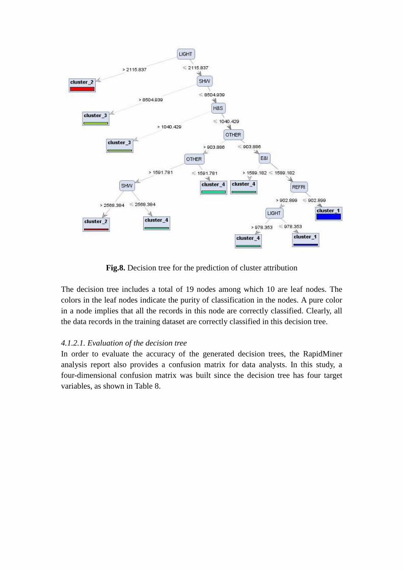
Fig.8. Decision tree for the prediction of cluster attribution
The decision tree includes a total of 19 nodes among which 10 are leaf nodes. The
colors in the leaf nodes indicate the purity of classification in the nodes. A pure color
in a node implies that all the records in this node are correctly classified. Clearly, all
the data records in the training dataset are correctly classified in this decision tree.
4.1.2.1. Evaluation of the decision tree
In order to evaluate the accuracy of the generated decision trees, the RapidMiner
analysis report also provides a confusion matrix for data analysts. In this study, a
four-dimensional confusion matrix was built since the decision tree has four target
variables, as shown in Table 8.

Table 8
Confusion matrix
Predicted data records
Cluster_1 Cluster_2 Cluster_3 Cluster_4
Actual
data
records
Cluster_1 7 0 0 0
Cluster_2 1 4 0 0
Cluster_3 1 0 1 0
Cluster_4 2 0 0 4
In this table, the rows indicate the number of actual data records used for testing in
each cluster; and the columns represent the number of predicted data records
generated by applying the decision tree to the actual data records. For example, the
first column shows that 7 records in cluster_1 were correctly classified; while one
record in cluster_2, one record in cluster_3, and two records in cluster_4 were
misclassified into cluster_1. Therefore, the accuracy of this decision tree, which is
also called ‘recall’ in the data mining domain, can be calculated as
(7+4+1+4)÷(7+4+1+4+1+1+2) = 80%, which is basically acceptable though
relatively low. This may be partly ascribed to the small size of database. Moreover,
data records in cluster_2, cluster_3, and cluster_4 are misclassified into cluster_1 (at
least one record in each cluster and four records totally), while data records in
cluster_1 are not misclassified into the other clusters. Such information indicates that
cluster_1 is more prone to be misclassified than the other clusters. This may have
occurred since nearly half of the data records in the database are in cluster_1, which
makes the decision tree more sensitive to this cluster. An even distribution among the
four clusters in the database would possibly improve the accuracy. In addition, the
sum of values in the matrix corresponds to the number of data records used for model
testing. Clearly 20 records in the database were randomly selected by RapidMiner for
testing, which also implies that 46 data records were used to establish the decision
tree.
4.1.2.3. Utilization of the decision tree
The decision tree can be utilized to predict the cluster attribution of new buildings
according to the main end-use loads. Such predictions can be easily made by
traversing a path from the root node to a leaf node. Take the node in the lower left
corner in Fig. 8 as an example. The prediction can be made as follows: for a building,
if LIGHT ≤ 2115.837 and SHW ≤ 8504.939 and H&S ≤ 1040.429 and
OTHER > 903.886 and OTHER > 1591.781 and SHW > 2568.384, then this building
belongs to cluster_2.
Besides the prediction of cluster attribution, useful information can also be extracted
from the decision tree so as to help understand building occupant behavior
improvement. For example, various attributes are selected by the decision tree

algorithm to split the nodes; and their degrees of closeness to the root node determines
the number of records impacted. Therefore, the closer an attribute is to the root node,
the more significant it affects the cluster attribution. Clearly the attribute significance
in the decision tree can be ranked as: LIGHT > SHW > H&S > OTHER > E&I >
REFRI. Such information indicates a general descending order of occupant behavior
deserving attention when modifying user activities in Japanese residential buildings.
Moreover, among the seven end-use loads, KITCH does not appear in the decision
tree. This may have occurred due to the narrow gap between energy consumption
caused by KITCH-related occupant behavior among the four clusters (see section
4.1.1), and thus KITCH has the weakest influence on the cluster attribution.
4.2. RB identification
In order to demonstrate the methodology, a case building with the most
comprehensive household appliances was selected for case study. Table 9 shows the
level 1 loads in this case building.
Table 9
End-use data in the case building (unit: MJ per capita per year)
SHW LIGHT KITCH REFRI E&I H&S OTHER Sum
3882.699 582.052 250.600 1541.394 1799.530 621.743 336.592 9014.610
Based on the decision tree, the cluster attribution of the case building can be predicted
as follows:
Step 1: Examine the value of LIGHT, i.e., the attribute in the root node. Since LIGHT
= 582.052, the node test in the right branch LIGHT ≤ 2115.837 is satisfied, then go
to the right-side child node;
Step 2: Examine the value of SHW. Since SHW = 3882.699, the node test in the right
branch SHW ≤ 8504.939 is satisfied, then go to the right-side child node;
Step 3: Examine the value of H&S. Since H&S = 621.743, the node test in the right
branch H&S ≤ 1040.429 is satisfied, then go to the right-side child node;
Step 4: Examine the value of OTHER. Since OTHER = 336.592, the node test in the
right branch OTHER ≤ 903.886 is satisfied, then go to the right-side child node;
Step 5: Examine the value of E&I. Since E&I = 1799.530, the node test in the left
branch E&I ≤ 1589.182 is satisfied, then go to the left-side child node, which is a
leaf node. As a result, the decision tree in Fig. 8 predicts that the case building
belongs to cluster_4.
Comparing with the other three clusters, cluster_4, as shown in Table 6, can be
characterized as the building group with high energy consumption in OTHER,
medium high energy consumption in REFRI and E&I. Therefore, the case building
occupants should manage to improve their behavior related to OTHER, REFRI, and
E&I.

After the prediction of cluster attribution, the sum of the seven main end-use loads in
the buildings in cluster_4 was calculated and ranked. Table 10 shows these loads and
their sum in the 14 buildings in cluster_4 in ascending order.
Table 10
The main end-use loads in the 14 buildings in cluster_4 (Unit: MJ per capita per year)
No. SHW LIGHT KITCH REFRI E&I H&S OTHER Sum
1 1691.656 744.428 1141.730 898.208 468.707 83.617 1670.297 6698.644
2 2757.408 981.880 662.657 645.977 388.737 317.828 1100.376 6854.487
3 1464.821 287.523 936.880 924.793 1958.911 504.171 845.352 6922.450
4 2471.123 865.524 1065.978 879.398 608.810 162.782 942.645 6996.259
5 1782.779 1099.852 322.597 1773.017 2092.484 142.018 556.186 7768.933
6 3337.796 558.252 411.807 1013.407 1060.430 360.339 1253.659 7995.690
7 3123.892 1094.065 1418.592 1055.741 803.612 160.549 1288.371 8944.821
8 2694.449 1758.554 621.970 1170.580 1109.116 503.125 1220.652 9078.446
9 3348.343 1407.656 1474.419 1046.065 768.032 550.396 739.591 9334.501
10 5224.677 617.440 724.771 565.889 498.162 186.758 1530.789 9348.487
11 4801.992 1080.952 994.315 909.184 870.845 202.665 818.539 9678.492
12 5192.053 982.723 768.211 777.985 363.490 923.699 1129.407 10137.568
13 5685.900 598.837 752.744 660.163 1007.248 269.102 1526.953 10500.947
14 2366.639 1089.153 451.300 2585.726 1878.995 817.197 2374.798 11563.808
A RB needs to be identified for the case building for the evaluation of energy-saving
potential and the improvement of occupant behavior. The buildings with less total
energy consumption (i.e. the sum of the seven main end-use loads) than the case
building in cluster_4 were considered to be RB candidates. In order to provide reliable
information for the case building occupants, the RB was defined as the most similar
building to the case building in terms of building-related parameters. The Euclidean
distance was used to determine the similarity. Various building-related parameters
were captured from the database to calculate the Euclidean distance. Among these
parameters, five are categorical parameters and are transformed into [0, 1], as shown
in Table 11.
Table 11
Transformation of categorical parameters
Categorical parameters CO HT Energy sources by usage
(SH, WH, KIT)
Value wood non-wood apartment detached house Electric non-electric
Transformation value 0 1 0 1 0 1
Table 12 shows the building-related parameters of the RB candidate buildings and the
case building.
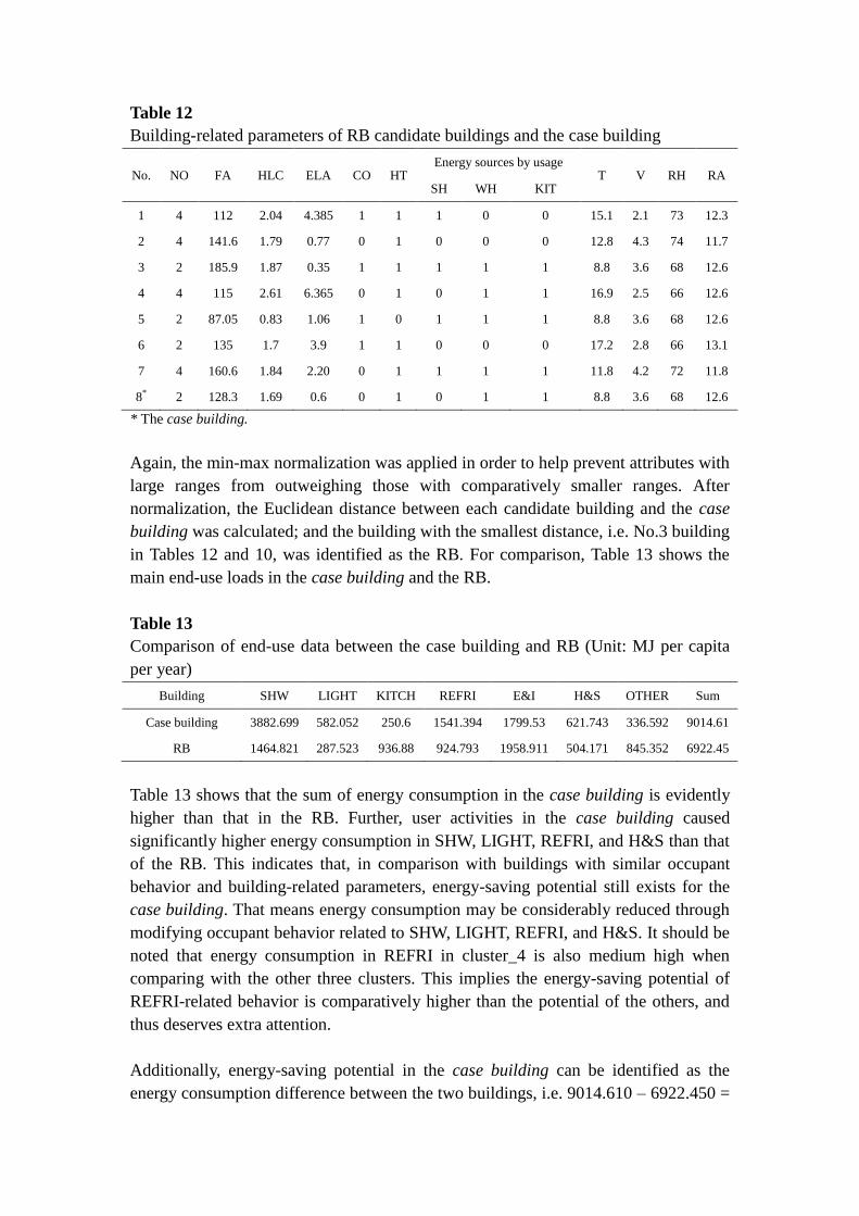
Table 12
Building-related parameters of RB candidate buildings and the case building
No. NO FA HLC ELA CO HT Energy sources by usage
T V RH RA SH WH KIT
1 4 112 2.04 4.385 1 1 1 0 0 15.1 2.1 73 12.3
2 4 141.6 1.79 0.77 0 1 0 0 0 12.8 4.3 74 11.7
3 2 185.9 1.87 0.35 1 1 1 1 1 8.8 3.6 68 12.6
4 4 115 2.61 6.365 0 1 0 1 1 16.9 2.5 66 12.6
5 2 87.05 0.83 1.06 1 0 1 1 1 8.8 3.6 68 12.6
6 2 135 1.7 3.9 1 1 0 0 0 17.2 2.8 66 13.1
7 4 160.6 1.84 2.20 0 1 1 1 1 11.8 4.2 72 11.8
8* 2 128.3 1.69 0.6 0 1 0 1 1 8.8 3.6 68 12.6
* The case building.
Again, the min-max normalization was applied in order to help prevent attributes with
large ranges from outweighing those with comparatively smaller ranges. After
normalization, the Euclidean distance between each candidate building and the case
building was calculated; and the building with the smallest distance, i.e. No.3 building
in Tables 12 and 10, was identified as the RB. For comparison, Table 13 shows the
main end-use loads in the case building and the RB.
Table 13
Comparison of end-use data between the case building and RB (Unit: MJ per capita
per year)
Building SHW LIGHT KITCH REFRI E&I H&S OTHER Sum
Case building 3882.699 582.052 250.6 1541.394 1799.53 621.743 336.592 9014.61
RB 1464.821 287.523 936.88 924.793 1958.911 504.171 845.352 6922.45
Table 13 shows that the sum of energy consumption in the case building is evidently
higher than that in the RB. Further, user activities in the case building caused
significantly higher energy consumption in SHW, LIGHT, REFRI, and H&S than that
of the RB. This indicates that, in comparison with buildings with similar occupant
behavior and building-related parameters, energy-saving potential still exists for the
case building. That means energy consumption may be considerably reduced through
modifying occupant behavior related to SHW, LIGHT, REFRI, and H&S. It should be
noted that energy consumption in REFRI in cluster_4 is also medium high when
comparing with the other three clusters. This implies the energy-saving potential of
REFRI-related behavior is comparatively higher than the potential of the others, and
thus deserves extra attention.
Additionally, energy-saving potential in the case building can be identified as the
energy consumption difference between the two buildings, i.e. 9014.610 – 6922.450 =

2092.161 MJ per capita per year.
4. 3. Association rule mining (ARM) in the case building
Based on the information obtained from cluster-then-classification and RB
identification, the ARM was then performed to find all the associations among the
end-use loads at both levels. Accordingly, energy-inefficient specific occupant
behavior will be determined and then energy-saving recommendations for modifying
activities can be provided for the case building occupants.
After experimenting with various combinations of support and confidence values, a
support of 50% and a confidence of 80% were set as minimum thresholds. Such
thresholds mean that, for each generated association rule, at least 50% of all the data
records under analysis contain both premise and conclusion; and the probability that a
premise’s emergence leads to a conclusion’s occurrence is 80% or more. In addition,
the minimum threshold of lift value was set 1 to find positive correlations. Such
mining generated 756 rules, many of which are obvious and uninteresting; and truly
interesting rules need to be further identified based on domain knowledge. Fifteen
association rules between household appliances were selected for demonstration
purposes, as shown in Table 14. It should be mentioned that most obtained
associations are between attributes in the LOW range (i.e. low energy consumption),
while clearly the associations in the HIGH range (i.e. high energy consumption) may
provide more useful information on energy conservation. This also indicates that the
attributes involved in the obtained rules have a skewed distribution toward the LOW
range, and may be ascribed to the high degree of building occupants’ energy-saving
consciousness. Moreover, due to the availability of the data source, daily data was
used for ARM instead of hourly data; and thus the obtained rules do not necessarily
indicate that user activities in the premises and conclusions occur simultaneously.
Therefore, the actual occupant behavior patterns should also be taken into
consideration when using these rules in practice.
Table 14
Selected association rules (min_supa*
= 50%, min_conf b*
= 80%, min_liftc*
=1)
No. Premise Conclusion Sup. Conf. Lift
Rule 1 Living room outlet [LOW] OTHER [LOW] 54% 98% 1.49
Rule 2 Heating boiler [HIGH] REFRI [HIGH] 51% 94% 1.12
Rule 3 Lamp 1F [LOW] LIGHT [LOW] 59% 96% 1.33
Rule 4 Washing machine 2F [LOW] H&S [LOW] 76% 97% 1.25
Rule 5 Dishwasher [LOW] KITCH [LOW] 74% 99% 1.26
Rule 6 Vacuum cleaner [LOW] H&S [LOW] 67% 84% 1.07
Rule 7 Microwave, toaster, coffee [LOW] KITCH [LOW] 66% 81% 1.04
Rule 8 TV (master bedroom 2F) [LOW] Lamp 2F [LOW] 66% 87% 1.10
Rule 9 TV (other rooms) [LOW] LIGHT [LOW] 51% 81% 1.11

Rule 10 Video [LOW] Table lamp [LOW] 52% 84% 1.02
Rule 11 Lamp 1F [LOW] Table lamp [LOW] 52% 84% 1.02
Rule 12 TV (Standby Power) [HIGH] Ventilator [HIGH] 55% 100% 1.82
Rule 13 Phone [LOW] Boom box [LOW] 57% 90% 1.06
Rule 14 TV (dining room) [LOW] Boom box [LOW] 51% 85% 1.01
Rule 15 TV (other rooms) [LOW] Boom box [LOW] 54% 86% 1.02
a* Minimum support, b* Minimum confidence, and c* Minimum lift.
The results of the cluster analysis show that the case building was grouped into
cluster_4, which was characterized as the building group with high energy
consumption in OTHER, medium high energy consumption in REFRI and E&I.
Hence, association rules involving OTHER, REFRI and E&I are the most important
and deserve more attention. Accordingly, two rules, i.e. Rule 1 and Rule 2 in Table 14,
were found among all the obtained rules and discussed as follows:
Rule 1 shows that living room outlet and OTHER have a strong positive association
with a confidence of 98% and a lift of 1.49. From this rule, it can be inferred that, in
this building, the electricity load increase in living room outlet would quite possibly
lead to the increase in OTHER. This indicates that, among all the unclear items
included in OTHER, removable electrically-operated devices connecting to the
living-room power plugs deserve more attention than other devices. Therefore,
building owners could easily identify these devices and then manage to modify their
usage to reduce energy consumption.
Rule 2 shows that heating boiler has a strong positive association with REFRI with a
confidence of 94% and a lift of 1.12. Given that the daily energy consumption of the
heating boiler is mainly impacted by occupant presence and outdoor air temperature,
this rule implies that, two factors (i.e. both a longer stay time of occupants and a
lower outdoor air temperature) possibly cause a higher energy consumption of
refrigerators. With regard to the first factor, it sounds reasonable since a longer stay
time of occupants tends to increase the refrigerator usage, thereby increasing the
energy consumption. With regard to the second factor, it seems unreasonable since a
low outdoor air temperature normally causes a relatively low indoor air temperature in
a detached house without central HVAC systems, thereby decreasing the energy
consumption of refrigerators. A possible explanation for this is that the building
occupants had high thermal comfort requirements in cold days; and preferred to a
high indoor air temperature by increasing the boiler thermostat setting or using
kerosene space-heaters. In order to justify the assumption, the pattern relating mean
daily kitchen air temperature1 to mean daily outdoor air temperature was plotted, as
shown in Fig. 9. A trend line was then drawn to find out whether the kitchen air
1In this building, both the kitchen and the living room are in the first floor, and there are no partitions between
them. Hence, they have the same indoor air temperature and the living room air temperature was used in this
figure.

temperature increased or decreased in relation to outdoor air temperature. Clearly, a
downward trend in mean daily kitchen air temperature following the increase of mean
daily outdoor air temperature can be observed, which is in accordance with the
assumption.
Fig.9. Mean daily air temperature in kitchen vs. mean daily outdoor air temperature
(winter, 2003)
Therefore, a trade-off between human thermal comfort and building energy
consumption is necessary for the owners, since an appropriate decrease of indoor
thermostat settings in cold days results in an energy-consumption reduction in both
space heating and refrigerators.
Further, the comparison between the RB and the case building shows that user
activities in the case building caused significantly higher energy consumption in SHW,
LIGHT, REFRI, and H&S than those in the RB. Hence, rules associating with these
four attributes also deserve extra attention. At the same time, in order to provide more
comprehensive recommendations for energy-efficient behavior, rules associating with
other end-use loads were also analyzed in this study. Eventually, thirteen interesting
rules (i.e. Rules 3 to 15 in Table 14) were selected and discussed as follows.
Similar to Rule 1, Rules 3, 4, and 5 show that lamp 1F, washing machine 2F and
dishwasher have a strong positive association with LIGHT, H&S, and KITCH,
respectively. Rules 6 and 7 show that vacuum cleaner, and microwave, toaster, coffee
have a positive association with H&S and KITCH, respectively. Therefore, comparing
with other appliances associating with LIGHT, H&S, and KITCH, the building
occupants should pay more attention to the use of lamps in the first floor, washing
machines in the second floor, and dishwashers, since activities related to these
appliances could have a major influence on the corresponding main end-use loads. At
the same time, the use of vacuum cleaners, microwave ovens, toasters, and coffee
machines also deserve some attention, though their associations with H&S and
KITCH are weaker than washing machine 2F and dishwasher.
Rule 8 shows that TV (master bedroom 2F) has a positive association with lamp 2F
20
20.5
21
21.5
22
22.5
23
23.5
24
-6 -5 -4 -3 -2 -1 0 1 2 3 4 5 6
Kit
chen
air
tem
pea
rtu
re (°C
)
Outdoor air temperature (°C)
with a confidence of 87% and a lift of 1.10. From this rule, it can be inferred that the
usage of TV (master bedroom 2F) would quite possibly lead to the usage of lamp 2F.
This may have occurred since the building occupants always turned the lights on
when they were watching TV. An effective way of reducing energy consumption in
this building is to watch TV with dim light.
Rules 9 to 11 can be explained in the same way as Rule 8 and similar
recommendations can be provided.
An unexpected result was that TV (Standby Power) and Ventilator have a strong
positive association with a confidence of 100% and a lift of 1.82, as shown in Rule 12.
Clearly the standby power of TVs and ventilators have the same trend of variation.
This may have occurred since the building occupants would turn off the TVs and
switch off the ventilators when the building was empty. However, standby power is
commonly unnecessary and still accounts for energy cost. Therefore, TVs should be
completely turned off or unplugged when they are not used. Furthermore, the wasted
standby power of TVs is very small, but the sum of standby use consumed by all
house appliances, such as microwave ovens, air conditioners, power adapters for
laptop computers and other electronic devices, becomes significant. Standby power
accounts for around 5-10% of residential electrical energy use in most developed
countries; and continues to increase in developing countries [21]. Hence, it is
meaningful to help building owners to realize the importance of reducing standby
power consumption, and feasible recommendations should also be provided for them.
For example, a switchable power strip can be used for multiple devices, such as VCRs,
DVD players, TVs, and computers, so that these appliances can be unplugged
conveniently with one action.
Rules 13 to 15 show that phone, TV (dining room) and TV (other rooms) have a
positive association with boom box. This indicates that, among all the appliances
included in E&I, boom boxes was used in comparatively high frequency and deserve
extra attention.
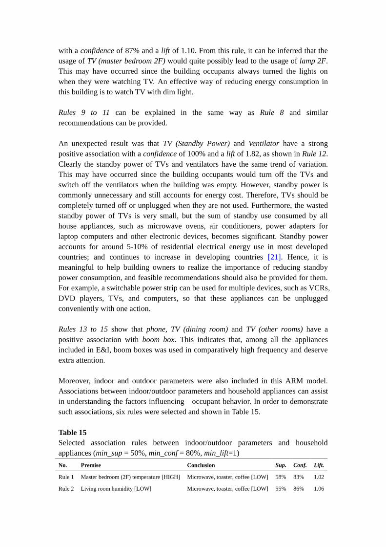
Moreover, indoor and outdoor parameters were also included in this ARM model.
Associations between indoor/outdoor parameters and household appliances can assist
in understanding the factors influencing occupant behavior. In order to demonstrate
such associations, six rules were selected and shown in Table 15.
Table 15
Selected association rules between indoor/outdoor parameters and household
appliances (min_sup = 50%, min_conf = 80%, min_lift=1)
No. Premise Conclusion Sup. Conf. Lift.
Rule 1 Master bedroom (2F) temperature [HIGH] Microwave, toaster, coffee [LOW] 58% 83% 1.02
Rule 2 Living room humidity [LOW] Microwave, toaster, coffee [LOW] 55% 86% 1.06

Rule 3 Outdoor relative humidity [LOW] Microwave, toaster, coffee [LOW] 57% 87% 1.07
Rule 4 Outdoor air temperature [LOW] H&S [LOW] 54% 88% 1.12
Rule 5 Outdoor air velocity [LOW] H&S [LOW] 59% 82% 1.05
Rule 6 Living room humidity [LOW] H&S [LOW] 57% 90% 1.15
Rules 1 to 3 show that master bedroom (2F) temperature (HIGH), living room
humidity, and outdoor relative humidity have a positive association with microwave,
toaster and coffee. This indicates that a high master bedroom temperature, as well as a
low living room or outdoor relative humidity, tends to decrease the usage of
microwave ovens, toasters, and coffee machines. A possible explanation for this is
that the increase in indoor air temperature, or the decrease in indoor/outdoor relative
humidity, causes the occupants to lose their appetite to some extent.
Rules 4 to 6 show that outdoor air temperature, outdoor air velocity, and living room
humidity have a positive association with H&S. This indicates that the decrease in
outdoor air temperature/velocity, and living room humidity tends to reduce the
likelihood that occupants do housework such as cleaning and washing. It can be
inferred that both local climatic conditions and indoor microclimate may have an
impact on occupant behavior relating to housework. For example, the increase of
outdoor air velocity may deteriorate indoor sanitary conditions (dust accumulation),
thereby increasing the usage of vacuum cleaners and other sanitary appliances.
In addition, based on all the generated rules, it was found that six attributes, as shown
in Table 16, have no association with the remaining attributes.
Table 16
Attributes without associations with the remaining attributes
No. Appliances Indoor parameters
1 Total energy consumption Living room temperature
2 I&E Bedroom (1F) temperature
3 Bidet
4 IH heater
The fact that these attributes have no association with the other attributes implies that,
in this building, they are independent. There are two possible reasons for these
attributes’ independence: for total energy consumption and I&E, they may be decided
by the holistic effects of various user activities, instead of associating with some
certain activity. For the other four attributes, their values may be purely random or
remain relatively stable in the whole winter and thus no association with other
attributes can be found. Such information can help building owners to make
intelligent decisions when modifying their behavior.

5. Conclusions
A methodology for identifying and improving occupant behavior in existing
residential buildings is developed. End-use loads of various household appliances
were mapped onto corresponding occupant behavior, and were used to deduce user
activities indirectly in this study. Specifically, these end-use loads were divided into
two levels (main and sub-category), and thus correspond to two-level activities, i.e.
general and specific occupant behavior.
In order to demonstrate its applicability, this methodology was applied to a group of
residential buildings located in six different districts of Japan. Field surveys on
energy-related data and other relevant information were carried out, and then a
database was developed. A building with the most comprehensive household
appliances was selected as the case building and the remaining buildings were used as
related buildings. Data pre-processing was performed for the related buildings and
they were grouped into four clusters by using K-means algorithm. The characteristic
of occupant behavior in each cluster was analyzed. Base on these clusters, a decision
tree was generated and its accuracy was evaluated as 80%. In terms of the decision
tree, the case building was predicted to belong to cluster_4. A reference building was
identified in the same cluster as the case building. Consequently, the case building
was compared with buildings in the other clusters and the reference building to
determine energy-inefficient general behavior. Also, its energy-saving potential was
identified as 2092.161 MJ per capita per year. Moreover, association rules were mined
based on the data of the case building in winter in 2003, given the seasonality of
occupant behavior. A number of interesting rules were found, and associations and
correlations between different user activities were discovered. According to these
rules, specific recommendations for highlighting energy-saving opportunities were
provided for the building occupants.
Considering the diversity of specific occupant behavior, the determination of
energy-inefficient general occupant behavior can narrow down the scope of
identification of energy-inefficient specific occupant behavior, and thus can help
occupants to quickly find the generated association rules, as well as specific behavior,
which deserve more attention. Also, such information is extracted from the real
measured data and covers almost all energy-related behavior. With such information,
building occupants can then clearly understand their actual behavior patterns, and
easily focus on the energy-inefficient behavior needing to be modified. Therefore, the
main advantage of the proposed methodology lies in its high efficiency of occupant
behavior improvement. Moreover, the identification of energy-inefficient general
behavior in this study is mainly based on the comparison with other similar buildings;
this can help building owners to be aware of avoidable energy waste caused by their
behavior, and motivate them to modify their activities accordingly.
The application of this proposed methodology to Japanese residential buildings in this

paper has clearly proved that this methodology is more efficient and rational than the
traditional methods, i.e. energy saving education method and building simulation
method. However, further study is still necessary and the main focus of future
research should be placed on identifying appropriate database sizes and the number of
clusters, improving the accuracy of generated decision tree. These measures have a
strong influence on characterizing the occupant behavior in all the investigated
buildings and cluster attribution of the case building. In addition, it is noted that using
daily end-use loads in the case building to mine associaton rules and provide
recommendations for occupants is not sufficient. This is because user activities in the
premises and conclusions of association rules may not occur simultaneously. In order
to overcome this limitation, hourly (or less than one hour, such as 15 minutes) end-use
loads of various household appliances should be measured and used in association
rule mining.
Acknowledgements
The authors would like to express their gratitude to the Public Works and Government
Services Canada, and Concordia University for the financial support. The authors also
wish to thank the reviewers for their valuable comments.
References
[1] Swan LG, Ugursal VI. Modeling of end-use energy consumption in the residential sector: A
review of modeling techniques. Renewable and Sustainable Energy Reviews 2009; 13(8):
1819–1835.
[2] Chen SQ, Li NP, Guan J, Xie YQ, Sun FM, Ni J. A statistical method to investigate national
energy consumption in the residential building sector of China. Energy and Buildings 2008; 40(4):
654–665.
[3] Tanatvanit S, Limmeechokchai B, Chungpaibulpatana S. Sustainable energy development
strategies: implications of energy demand management and renewable energy in Thailand.
Renewable and Sustainable Energy Reviews 2003; 7(5): 367–395.
[4] Ruijven BV, Vries BD, Van Vuuren DP, Van der Sluijs JP. A global model for residential energy
use: Uncertainty in calibration to regional data. Energy 2010; 35(1): 269–282.
[5] Shimoda Y, Asahi T, Taniguchi A, Mizuno M. Evaluation of city-scale impact of residential
energy conservation measures using the detailed end-use simulation model. Energy 2007; 32(9):
1617–1633.
[6] Kenisarin M, Kenisarina K. Energy saving potential in the residential sector of Uzbekistan.
Energy 2007; 32(8): 1319–1325.[7] Yu Z, Fung BCM, Haghighat F, Yoshino H, Morofsky E. A
systematic procedure to study the influence of occupant behavior on building energy consumption.
Energy and Buildings 2011; 43(6): 1409–1417
[8] Ouyang JL, Hokao K, Energy-saving potential by improving occupants' behavior in urban
residential sector in Hangzhou City, China. Energy and Buildings 2009; 41(7): 711–720.
[9] Al-Mumin A, Khattab O, Sridhar G. Occupants' behavior and activity patterns influencing the
energy consumption in the Kuwaiti residences. Energy and Buildings 2003; 35(6): 549–559.
[10] Zmeureanu R, Fazio P, DePani S, Calla R. Development of an energy rating system for

existing houses. Energy and Buildings 1999; 29(2): 107–119.
[11] Han JW, Kamber M. Data Mining Concepts and Techniques. 2nd ed. San Francisco: Elsevier
Inc; 2006.
[12] Yu Z, Haghighat F, Fung BCM, Yoshino H. A decision tree method for building energy
demand modeling, Energy and Buildings (2010); 42(10): 1637–1646.
[13] Rapid – I – RapidMiner. http://rapid-i.com/content/view/181/190/
[14] Davies DL, Bouldin DW. A cluster separation measure, IEEE Trans Pattern Anal Mach
Intelligence 1979; 1: 224–227.
[15] Quinlan JR. Induction of decision trees. Machine Learning 1986; 1: 81-106.
[16] L.Breiman, J.H.Friedman, R.A.Olshen, C.J.Stone, Classification and Regression Trees. 2nd
ed. Belmont: Wadsworth Inc.; 1984.
[17] J.R. Quinlan. C4.5 Programs for Machine Learning. 1st ed. San Mateo: Morgan Kaufmann;
1993.
[18] Association Rule Mining with WEKA.
http://maya.cs.depaul.edu/~Classes/Ect584/Weka/associate.html
[19] Murakami S, Akabayashi S, Inoue T, Yoshino H, Hasegawa K, Yuasa K, Ikaga T, Energy
consumption for residential buildings in Japan, Architectural Institute of Japan, Maruzen Corp.,
2006 (http://tkkankyo.eng.niigata-u.ac.jp/HP/HP/database/index.htm).
[20] Helsel DR, Hirsch RM. Statistical methods in water resources. U.S. department of the interior
2002
[21] Standby Power, Frequently Asked Questions (FAQs). http://standby.lbl.gov/faq.html