A Methodology for Capturing the Impacts of Bleed Flow ... · A Methodology for Capturing the Impacts of Bleed Flow Extraction on Compressor Performance and Operability in Engine Conceptual

A Methodology for Capturing the Impacts of Bleed Flow Extraction on

Compressor Performance and Operability in Engine Conceptual Design

A Thesis

Presented to

The Academic Faculty

By

JOSHUA DANIEL BROOKS

In Partial Fulfillment

Of the Requirements for the Degree

Master of Science

School of Aerospace Engineering

Georgia Institute of Technology

May 2015

Copyright © Joshua D Brooks 2015

A Methodology for Capturing the Impacts of Bleed Flow Extraction on

Compressor Performance and Operability in Engine Conceptual Design

Approved by:

Professor Dimitri Mavris, Avisor



Dr. Jeff Schutte



Dr. Jimmy Tai



Mr. Russell Denney



Date Approved: April 17, 2015

DEDICATION

I would like to dedicate this thesis and all of the work herein to my family, my

soon to be bride, Jessica, my two loving sisters, Ashley and Amy, and my incredible

parents, Robert and Katherine, who have provided me with consistent encouragement and

unconditional support throughout the duration of this endeavor.

Additionally I would like to dedicate this work to my family in Atlanta, Conrad,

Jessica, Joanna, Molly, and William Brooks, who selflessly provided for me in care,

fellowship, support, guidance, friendship, and above all else, love. Love like this can only

come from one place, which leads me to my most important dedication of all.

It brings me the greatest joy to dedicate, and fully credit this work to my Lord and

Savior, Jesus Christ.

“Whatever you do, do your work heartily, as for the Lord rather than for men…it is the

Lord Christ whom you serve” – Colossians 3:23

Through his blessings alone, I was able to attend this institution, and through his

blessings alone I was able to produce this work.

“But in all these things we overwhelmingly conquer through Him who loved us. For I am

convinced that neither death, nor life, nor angels, nor principalities, nor things present,

nor things to come, nor powers, nor height, nor depth, nor any other created thing, will

be able to separate us from the love of God, which is in Christ Jesus our Lord.”

– Romans 8:37-39

iv

ACKNOWLEDGEMENTS

I would like to thank Dr. Dimitri Mavris for his guidance and support as my

committee chairman throughout the course of this work. His provision for this

experience, from believing in me enough to bring me into the ASDL, to encouraging me

to complete this research, has been a wonderful blessing in my life.

I would like to thank Dr. Jeff Schutte, Dr. Jimmy Tai, and Mr. Russell Denney for

serving on my committee, and for their continued encouragement and technical support

throughout the completion of this endeavor.

I would like to thank my friends at the ASDL, especially Andrew Miller for his

technical advice and fellowship in this work.

Finally, I would like to thank my many mentors from my undergraduate work

until now, who have inspired my research interests and who stand as role models for my

technical work. These include, amongst others, Dr. Jeffrey Moore, Dr. Jason Wilkes, Dr.

Luis San Andres, Dr. Devesh Ranjan, Dr. Brian Kestner, and Dr. Simon Briceno.

v

TABLE OF CONTENTS

DEDICATION ................................................................................................................................ iii

ACKNOWLEDGEMENTS ............................................................................................................ iv

LIST OF TABLES ......................................................................................................................... vii

LIST OF FIGURES ...................................................................................................................... viii

LIST OF ABBREVIATIONS AND SYMBOLS ........................................................................... xi

SUMMARY ................................................................................................................................... xii

CHAPTER 1: INTRODUCTION .................................................................................................... 1

Motivation .................................................................................................................................... 2

CHAPTER II: BACKGROUND ................................................................................................... 11

Axial Compressor System.......................................................................................................... 11

SFTF Engine System ................................................................................................................. 22

Compressor Performance Map Genesis ..................................................................................... 26

Research Questions .................................................................................................................... 30

CHAPTER III: METHODOLOGY ............................................................................................... 34

Experiment 1 .............................................................................................................................. 34

Experiment 2 .............................................................................................................................. 41

Experiment 3 .............................................................................................................................. 46

Experiment 4 .............................................................................................................................. 50

CHAPTER IV: RESULTS ............................................................................................................. 54

Experiment 1 .............................................................................................................................. 54

Experiment 2 .............................................................................................................................. 64

Model Construction ............................................................................................................... 65

Model Implementation and Assessment ................................................................................ 79

Experiment 3 .............................................................................................................................. 82

Design of Experiments ........................................................................................................... 83

Response Surface Equations .................................................................................................. 87

RSE Implementation and Assessment ................................................................................... 94

Experiment 4 ............................................................................................................................ 100

Engine Cycle Analysis ......................................................................................................... 101

RSE Integration .................................................................................................................... 103

vi

Full System Assessment ...................................................................................................... 104

CHAPTER V: CONCLUSIONS ................................................................................................. 113

Research Questions .............................................................................................................. 113

Recommendations ................................................................................................................ 118

APPENDIX A: ERROR AND UNCERTAINTY ANALYSES .................................................. 119

APPENDIX B: DoE and RSE TABLES AND FIGURES .......................................................... 120

REFERENCES ............................................................................................................................ 131

vii

LIST OF TABLES

Table 1: Parameter variation for design of experiments ................................................... 48

Table 2: Operating conditions for assessment one of experiment one. ............................ 55

Table 3: Operating conditions for assessment two of experiment one. ............................ 57

Table 4: Comparison of variable to fixed geometry prediction performance. .................. 59

Table 5: Sample of full LHD DoE. ................................................................................... 85

Table 6: Surrogate evaluation cases. ................................................................................. 98

Table 7: Experiment 3: Design of Experiments .............................................................. 120

Table 8: Summary of R2 values ...................................................................................... 122

viii

LIST OF FIGURES

Figure 1: Simple diagram of a separate flow turbofan engine. (SFTF) .............................. 2

Figure 2: Specific Fuel Consumption Reduction with Engine Bypass Ratio. [5] .............. 4

Figure 3: New engine BPR increase over time. [62] .......................................................... 5

Figure 4: Physical implications of increased BPR engines. [7] .......................................... 7

Figure 5: Operability impact of bleed flow extraction on the axial compressor. [27] ........ 9

Figure 6: Axial Compressor with two bleed extraction ports. .......................................... 12

Figure 7: Photograph of an axial compressor rotor. [78] .................................................. 13

Figure 8: Full compressor pressure ratio performance mapping. ..................................... 15

Figure 9: Full compressor efficiency performance mapping. ........................................... 15

Figure 10: Initiation of boundary layer separation as mass flow is reduced. ................... 18

Figure 11: Pressure ratio variation with VSV settings...................................................... 21

Figure 12: Efficiency variation with VSV settings. .......................................................... 22

Figure 13: Notional cycle analysis component organization for a SFTF. ........................ 23

Figure 14: Compressor map traverse with bleed variation. .............................................. 26

Figure 15: Axial compressor broken into individual stages. ............................................ 27

Figure 16: Flow deflection through a single compressor stage. ....................................... 36

Figure 17: Radial cross section of the full E3 compressor. ............................................... 37

Figure 18: VSV schedule used during the B1 testing of the E3 B1 testing. ...................... 38

Figure 19: Full compressor performance map from B1 testing of E3 ............................... 39

Figure 20: Bleed extraction at the full compressor level. ................................................. 42

Figure 21: Bleed extraction at the interstage level. ........................................................... 43

Figure 22: VSV schedule utilized by the E3 B2 compressor testing................................. 44

Figure 23: Full compressor mapping constructed from the E3 B2 testing. ....................... 44

Figure 24: Parameterized map updated in the engine cycle analysis................................ 51

Figure 25: Example of VSV angle amendment with increased rotation. ......................... 54

Figure 26: Pressure ratio mapping for the fixed geometry model condition. ................... 56

Figure 27: Efficiency mapping for the fixed geometry model condition. ........................ 56

Figure 28: Pressure ratio mapping for the variable geometry model condition. .............. 58

ix

Figure 29: Efficiency mapping for the variable geometry model condition. .................... 58

Figure 30: NACA 8 Stage performance mapping for VSV impact exploration. .............. 61

Figure 31: Performance mapping for VSV impact exploration using the E3 B1 model. .. 62

Figure 32: Pressure ratio mapping of the E3 B1 model. ................................................... 63

Figure 33: Efficiency mapping of the E3 B1 model. ......................................................... 64

Figure 34: Expansion of a single streamline in OTAC. .................................................... 66

Figure 35: Bleed flow extraction from a modeling standpoint. ........................................ 68

Figure 36: Thermodynamic response to bleed flow extraction. ....................................... 69

Figure 37: Predicted bleed flow extraction in a two stage compressor. ........................... 71

Figure 38: Stage stacking of performance mappings in the presence of bleed. ................ 73

Figure 39: Tip stream bleed profile. ................................................................................. 74

Figure 40: Equal division bleed profile. ........................................................................... 75

Figure 41: Bleed profile trade study at 1% and 3% bleed. ............................................... 76

Figure 42: Static drop comparison at 3% bleed flow extraction. ...................................... 77

Figure 43: Static pressure drop comparison at 1% bleed flow extraction. ....................... 78

Figure 44: Empirical data from the E3 B1 and B2 testing. ............................................... 80

Figure 45: E3 B1 compressor pressure ratio under the B2 conditions. ............................. 81

Figure 46: E3 B1 compressor efficiency under the B2 conditions. ................................... 82

Figure 47: DoE design space coverage. ............................................................................ 85

Figure 48: OTAC point to point solver behavior. ............................................................. 86

Figure 49: Flow establishment for RSE operation. ........................................................... 90

Figure 50: Actual by predicted plot for the 97.5% PR surrogate. ..................................... 93

Figure 51: Residual by predicted plot for the 97.5% PR surrogate. ................................. 93

Figure 52: Model Fit Error (left) Model Representation Error (Right) ............................ 94

Figure 53: Surrogate predicted pressure ratio comparison. .............................................. 96

Figure 54: Surrogate Predicted efficiency comparison. .................................................... 97

Figure 55: evaluation of surrogate pressure ratio across extreme operating conditions. .. 98

Figure 56: evaluation of surrogate efficiency across extreme operating conditions. ....... 99

Figure 57: Core component representation of SFTF engine cycle analysis. .................. 102

Figure 58: User ability to select bleed handling method. ............................................... 104

Figure 59: Pressure ratio mapping impact with the addition of bleed. ........................... 106

x

Figure 60: Efficiency mapping impact with the addition of bleed. ................................ 107

Figure 61: Pressure ratio performance predictions from both bleed handling methods. 108

Figure 62: Efficiency performance predictions from both bleed handling methods. ..... 109

Figure 63: Comparison of TSFC for all three cases. ...................................................... 110

Figure 64: Stall margin comparison for each of the three cases. .................................... 112

Figure 65: Stall Flow at 97.5% design speed. ................................................................. 123

Figure 66: Stall Flow at 95% design speed. .................................................................... 123

Figure 67: Stall Flow at 92.5% design speed. ................................................................. 124



Figure 70: Pressure Ratio at 97.5% design speed. .......................................................... 125

Figure 71: Pressure Ratio at 95% design speed. ............................................................. 126

Figure 72: Pressure Ratio at 92.5% design speed. .......................................................... 126



Figure 75: Efficiency at 97.5% design speed.................................................................. 128

Figure 76: Efficiency at 92.5% design speed.................................................................. 128

Figure 77: Efficiency at 95% design speed..................................................................... 129



Figure 80: Full range of VSV schedule settings. ............................................................ 130

xi

LIST OF ABBREVIATIONS AND SYMBOLS

ASDL Aerospace Systems Design Laboratory

BPR Engine Bypass Ratio

B5 Fifth Stage Bleed Location

B7 Seventh Stage Bleed Location

DoE Design of Experiments

𝐹𝐶𝐶𝐶𝐷 Face Centered Central Composite Design

𝐹𝑃𝑅 Fan Pressure Ratio

𝐼𝐺𝑉 Inlet Guide Vane

𝐿𝐻𝐷 Latin Hypercube Design

𝑂𝑃𝑅 Overall Pressure Ratio

𝑂𝑇𝐴𝐶 Object-oriented Turbomachinery Analysis Code

𝑆𝐹𝐶 Specific Fuel Consumption

𝑇𝑆𝐹𝐶 Thrust Specific Fuel Consumption

𝑇𝐸𝑇 Turbine Entrance Temperature

𝑉𝑆𝑉 Variable Stator Vane

𝐹𝐻𝑉 Fuel Heating Value

𝑉𝑂 Ambient Air Velocity [ft/s]

𝛼1 Absolute flow angle at compressor inlet

𝛼2 Absolute flow angle at compressor outlet

𝛽1 Relative flow angle at compressor inlet

𝛽2 Relative flow angle at compressor outlet

𝜂𝑇 Thermal Efficiency

𝜂𝑃 Propulsive Efficiency

xii

SUMMARY

The commercial aviation industry continually faces the challenge of reducing fuel

consumption for the next generation of aircraft. This challenge rests largely on the

shoulders of engine design teams, who push the boundaries of the traditional design

paradigm in pursuit of more fuel efficient, cost effective, and environmentally clean

engines. In order to realize these gains, there is a heightened requirement of accounting

for engine system and subsystem level impacts from a wide range of variables, earlier in

the design process than ever before. One of these variables, bleed flow extraction, or

simply bleed, plays an especially greater role; due to the approach engine designers are

taking to combat the current state of fuel efficiency. For this reason, this research

examined the current state of bleed handling performed during the engine conceptual

design process, questioned its adequacy with regards to properly capturing the impacts of

this mechanism, and developed a bleed handling methodology designed to replace the

existing method.

The traditional method of handling bleed in the engine cycle design stage relies

on a variety of engine level impacts stemming from zero dimensional thermodynamic

analysis, as well as the utilization of a static performance characterization of the engine

compression component, the axial flow compressor. The traditional method operates

under the assumption that the introduction of additional bleed to the compressor system

has created no additional compressor level impact. The methodology developed in this

work challenges this assumption in two parts, first by creating a way to evaluate the

compressor level impacts caused by the introduction of bleed, and second by

xiii

implementing the knowledge gained from this compressor level evaluation into the

engine cycle design, where the engine level impacts could be compared to those predicted

by the traditional method of bleed handling.

The compressor level impacts from the addition of bleed were quantified using a

low fidelity, multi-stream, meanline analysis. Here, an innovative approach was

developed which cross pollinated existing methods used elsewhere in the analysis

environment, to account for the bleed impact in the object oriented modeling

environment. Implementation of this approach revealed that the addition of bleed

negatively and significantly impacts the compressor level performance and operability.

With the completion of the above analyses, this newly acquired capability to

quantify, or at least qualify, the compressor level bleed impacts was tied into the engine

level cycle analysis. This form of component zooming, allows the user to update the

bleed flow rate from a number of locations along the compressor, as well as the

compressor variable stator vain orientation, within the existing cycle analysis. Utilization

of this ability provided engine level performance and operability analyses which revealed

a disparity between the traditional and herein developed bleed handling methodology’s

predictions. The found results reveal a need for more stringent handling of bleed during

the engine conceptual design than the traditional method provides, and suggests that the

developed methodology provides a positive step to the realization of this need.

1

CHAPTER 1: INTRODUCTION

The World’s most common propulsive mechanism used for powering modern

aircraft is the gas turbine engine. The gas turbine engine is a complex mechanical device

that converts the chemical energy in fuel into useful shaft work, accelerating large

amounts of air to propel an aircraft [26]. The separate flow turbofan (SFTF), shown in

Figure 1, is a type of gas turbine engine which utilizes two main air streams, one

traveling through the core of the machine and the other through a bypass duct around the

core, driven by a fan at the front of the engine. This configuration allows for a large

increase in thrust, provided by the addition of the fan, at the cost of a small increase in

fuel, equating to a gain in propulsive efficiency, and a net gain in overall engine

efficiency [74]. Because of the efficiency of the SFTF, as well as its operating range with

respect to performance and airspeed, it has become the most common engine of choice in

the commercial aviation industry. Due to this reputation, the SFTF will be the type of

engine analyzed in this thesis.

Although the central purpose of a gas turbine engine is to generate the thrust

necessary for a specific aircraft mission, these machines are also utilized for bleed flow

and shaft work extraction [30]. Bleed flow extraction is the process of drawing air from

the engine compressor for use elsewhere in the engine or onboard the aircraft, and shaft

work (horse power) extraction converts shaft work from the engine to be used onboard

the aircraft. Both of these processes draw energy away from that which would be

otherwise available for thrust generation, which impacts the performance of the core of

the engine [6]. Of particular interest to this work, is the qualification of specific impacts

2

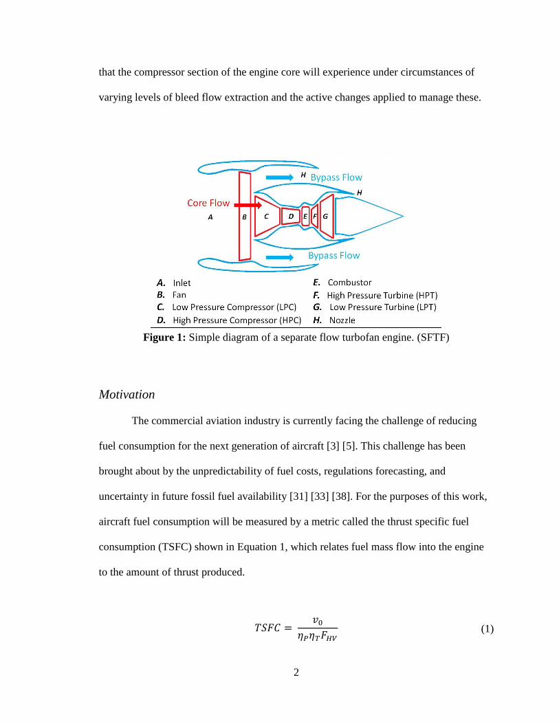
that the compressor section of the engine core will experience under circumstances of

varying levels of bleed flow extraction and the active changes applied to manage these.

Figure 1: Simple diagram of a separate flow turbofan engine. (SFTF)

Motivation

The commercial aviation industry is currently facing the challenge of reducing

fuel consumption for the next generation of aircraft [3] [5]. This challenge has been

brought about by the unpredictability of fuel costs, regulations forecasting, and

uncertainty in future fossil fuel availability [31] [33] [38]. For the purposes of this work,

aircraft fuel consumption will be measured by a metric called the thrust specific fuel

consumption (TSFC) shown in Equation 1, which relates fuel mass flow into the engine

to the amount of thrust produced.

𝑇𝑆𝐹𝐶 = 𝑣0

𝜂𝑃𝜂𝑇𝐹𝐻𝑉 (1)

3

Both the engine and the airframe of the aircraft are responsible for inefficiencies

in fuel consumption. However, since the engine is directly consuming the fuel, there is an

arguably larger burden placed on the shoulders of engine designers to reduce the overall

fuel consumption, or at the engine level, the TSFC. In pursuit of realizing this reduction,

there are three approaches historically available to engine cycle designers.

The first two approaches require either increasing the overall pressure ratio

(OPR) or increasing the turbine entrance temperature (TET) [4]. The OPR is a measure of

the total pressure rise between the air entering the engine and the combustor, while the

TET is the temperature of the air when it enters the turbine section. The associated TSFC

improvement is generated from the fact that the thermal efficiency (𝜂𝑇) of the engine is

increased when increasing the OPR or the TET, shown in Equation 2 [83]. This increase

in thermal efficiency, as Equation 1 shows, results in a reduction of the engine TSFC [1].

𝜂𝑇 ≈ 1 − 1

𝑂𝑃𝑅 ≈ 1 −

1

𝑇𝐸𝑇 (2)

Unfortunately, these two approaches for improving engine TSFC are constrained

by blade cooling requirements, blade materials, and component performance [3]. Of

particular challenge in these is finding materials with improved temperature capabilities,

which still possess the strength, creep resistance, and fatigue qualities required for the

extreme environment of a gas turbine engine [3]. These constraints direct this work to the

third and final approach for decreasing engine TSFC, performed through an increase of

the engine bypass ratio (BPR), which is the ratio of airflow in the bypass stream to the

airflow in the core stream, shown in Equation 3 [4].

4

BPR =

Bypass Mass Flow

Core Mass Flow (3)

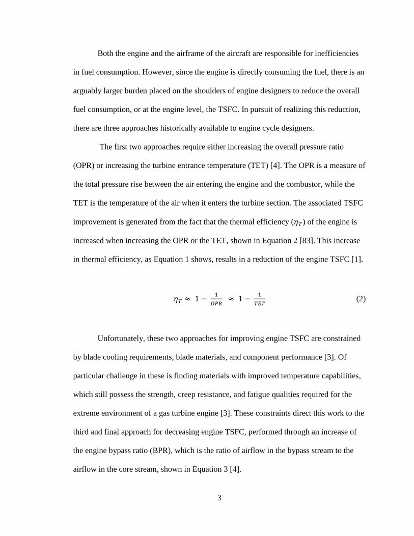
Increasing the BPR is performed in order to increase the propulsive efficiency

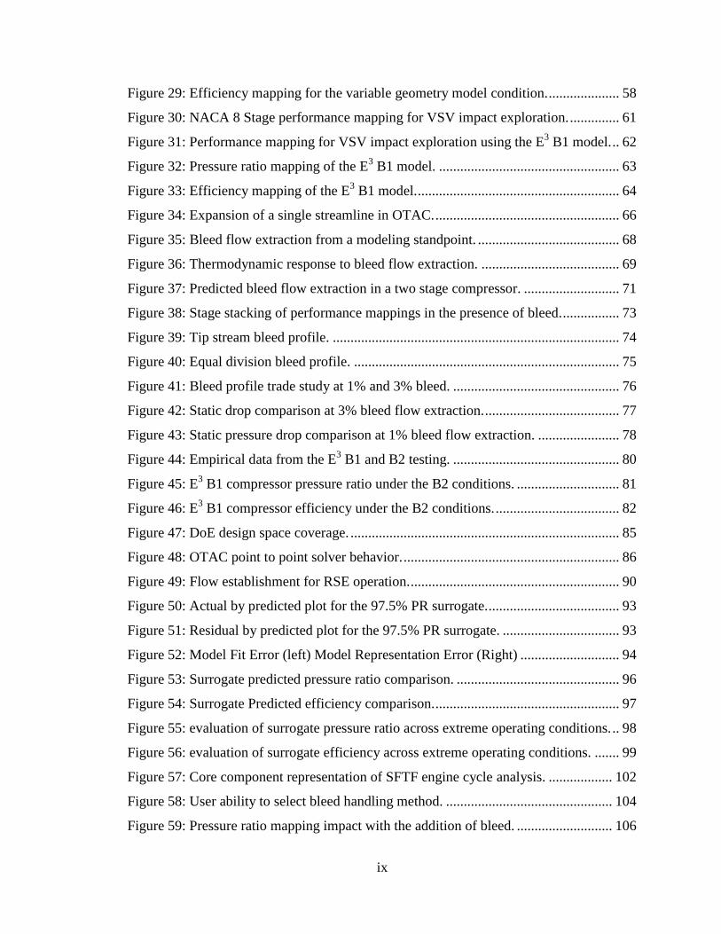
(𝜂𝑃) of the engine, shown in Equation 4 [4]. This increase in propulsive efficiency, as

Equation 1 shows, results in a reduction of the engine TSFC [1]. Additionally, this

reduction of TSFC produced by an increase in BPR is shown in Figure 2 [5].

𝜂𝑃 =

𝑐0 ∗ (𝑐1 + 𝐵𝑃𝑅 (𝑐2) − (1 + 𝐵𝑃𝑅) ∗ 𝑐0)𝑐12

2+ 𝐵𝑃𝑅 ∗

𝑐22

2− (1 + 𝐵𝑃𝑅) ∗

𝑐02

2

(4)

Figure 2: Specific Fuel Consumption Reduction with Engine Bypass Ratio. [5]

JT3D JT8D - 1

JT8D-200 JT9D - 3A

JT9D - 7A

JT9D - 7R4G

PW4168 PW4084

V2500

PW2000 PW4000

0.5

0.55

0.6

0.65

0.7

0.75

0.8

0.85

0 2 4 6 8

TS

FC

Bypass Ratio

5

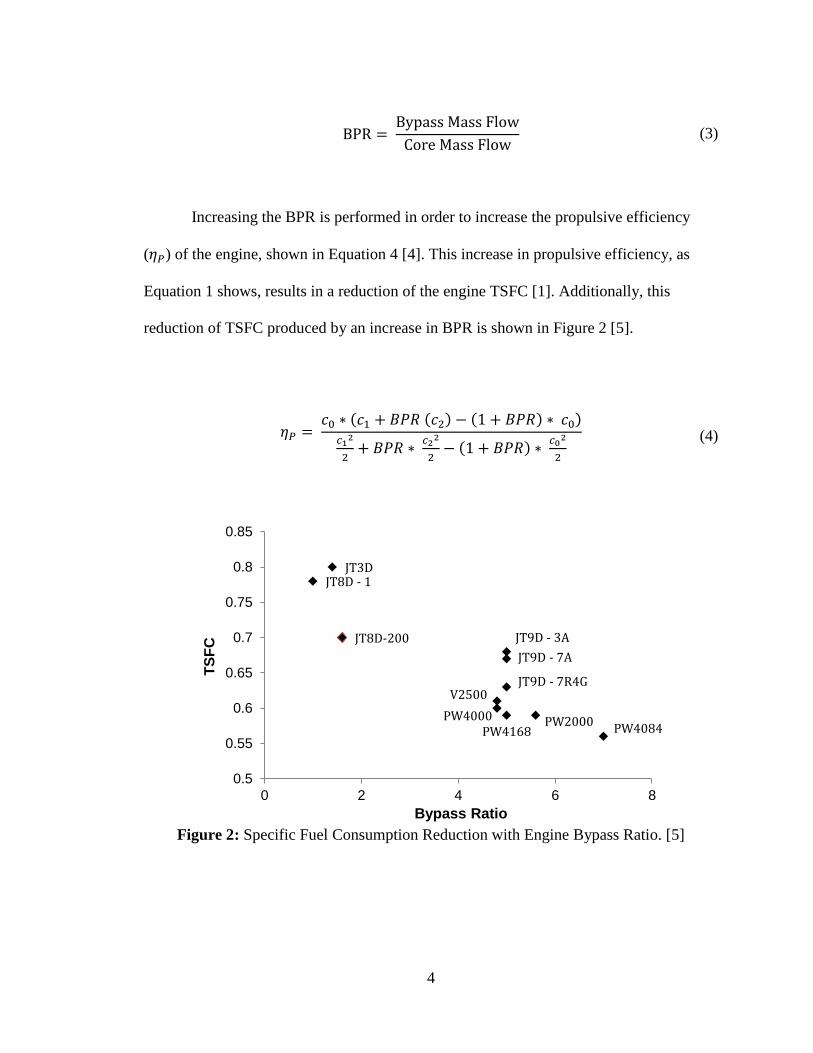
The effectiveness of this approach for reducing engine TSFC has historically

made it a popular choice of engine designers [1]. This trend is apparent in the historical

data for production of higher BPR engines over time, displayed in Figure 3 [62]. Due to

the proven success of this approach and the consistently increasing trend that can be seen

in Figure 3, it is assumed that the popularity of this approach will continue to grow, with

engine manufacturers producing higher and higher bypass ratio engines in the foreseeable

future.

Figure 3: New engine BPR increase over time. [62]

0

2

4

6

8

10

12

1950 1970 1990 2010 2030

En

gin

e B

yp

as

s

Rati

o

Service Entry (Year)

Today

6

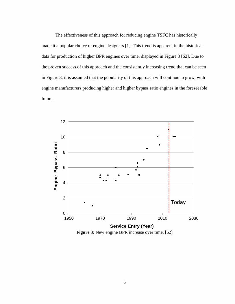
Increasing the engine BPR introduces a new set of multidisciplinary challenges.

These challenges include stability and control issues as well as drag and weight penalties

caused by a larger and likely heavier engine, as well as the geometrical constraints to the

maximum size of the fan diameter [7] [71]. Shown in Equation 3, there are two ways to

increase the engine bypass ratio: increase the flow through the bypass duct, or decrease

the flow through the core. Increasing the flow through the bypass duct requires a larger

fan, the size of which being constrained by installation issues among the other challenges

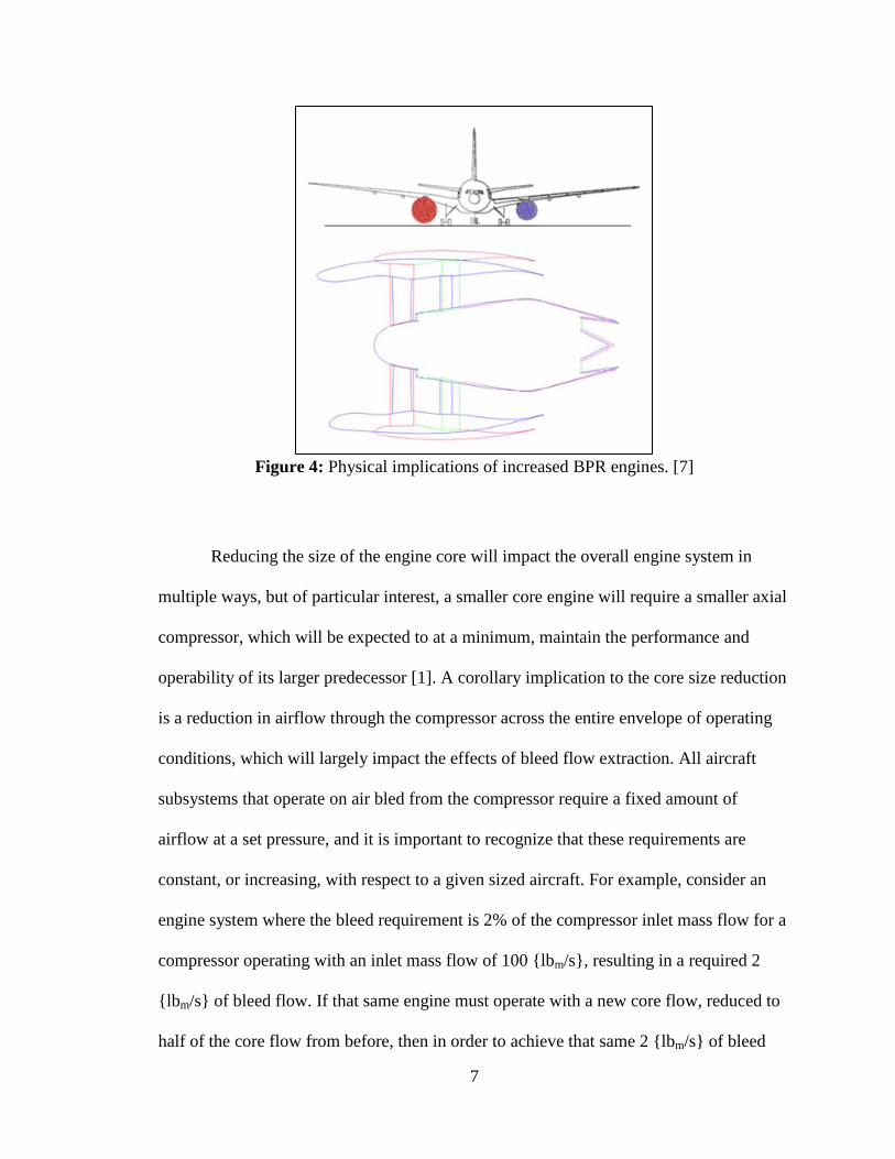
from before [7]. Figure 4 shows a notional engine cross section with an increased BPR,

accomplished through a larger fan diameter, and the implication this change would have

on the engine installation due to ground clearance regulations [7]. There simply is not

enough space to expand, given the current airframe configuration, and because of this

constraint on maximum fan diameter, increases in BPR will likely need to be achieved

through the opposite approach. This means engine designers will need to trade engine

core flow for increased bypass flow, resulting in a net reduction in airflow through the

engine core [1] [7]. This reduction in core flow allows for an increase in BPR,

constrained to a maximum fan diameter, at the cost of a reduced engine core size.

7

Figure 4: Physical implications of increased BPR engines. [7]

Reducing the size of the engine core will impact the overall engine system in

multiple ways, but of particular interest, a smaller core engine will require a smaller axial

compressor, which will be expected to at a minimum, maintain the performance and

operability of its larger predecessor [1]. A corollary implication to the core size reduction

is a reduction in airflow through the compressor across the entire envelope of operating

conditions, which will largely impact the effects of bleed flow extraction. All aircraft

subsystems that operate on air bled from the compressor require a fixed amount of

airflow at a set pressure, and it is important to recognize that these requirements are

constant, or increasing, with respect to a given sized aircraft. For example, consider an

engine system where the bleed requirement is 2% of the compressor inlet mass flow for a

compressor operating with an inlet mass flow of 100 {lbm/s}, resulting in a required 2

{lbm/s} of bleed flow. If that same engine must operate with a new core flow, reduced to

half of the core flow from before, then in order to achieve that same 2 {lbm/s} of bleed

8

flow, a now greater 4% of the compressor inlet mass flow is required. This means that the

core flow available for bleed flow extraction is considerably more expensive than before,

necessitating a more intensive evaluation of this mechanism at both the compressor level

and the engine level.

Bleed extraction has multiple impacts on the performance and operability of both

the compressor and the engine system [6]. For a given engine and inter-stage bleed

location, increasing the inter-stage bleed flow rate (the amount of air extracted), results in

a lower specific thrust and pressure rise across the engine, and a higher engine TSFC [6]

[42]. In addition, increasing the bleed flow rate results in the operating point of the

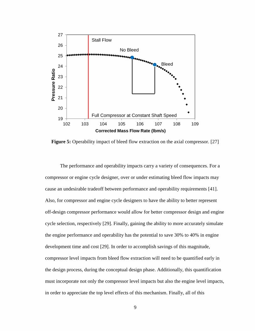
compressor moving further away from the point of stall shown in Figure 4, which is a

notional representation that may be found from a compressor rig test conducted at a

constant rotational speed [40].

9

Figure 5: Operability impact of bleed flow extraction on the axial compressor. [27]

The performance and operability impacts carry a variety of consequences. For a

compressor or engine cycle designer, over or under estimating bleed flow impacts may

cause an undesirable tradeoff between performance and operability requirements [41].

Also, for compressor and engine cycle designers to have the ability to better represent

off-design compressor performance would allow for better compressor design and engine

cycle selection, respectively [29]. Finally, gaining the ability to more accurately simulate

the engine performance and operability has the potential to save 30% to 40% in engine

development time and cost [29]. In order to accomplish savings of this magnitude,

compressor level impacts from bleed flow extraction will need to be quantified early in

the design process, during the conceptual design phase. Additionally, this quantification

must incorporate not only the compressor level impacts but also the engine level impacts,

in order to appreciate the top level effects of this mechanism. Finally, all of this

19

20

21

22

23

24

25

26

27

102 103 104 105 106 107 108 109

Pre

ss

ure

Ra

tio

Corrected Mass Flow Rate (lbm/s)

Stall Flow

No Bleed

Bleed

Full Compressor at Constant Shaft Speed

10

information must be collected into a form capable of answering the overarching issue

driving this research.

Problem Statement: In the conceptual design phase, how does one determine the

minimum core size to meet compressor performance and operability while accounting

for subsystem bleed requirements?

11

CHAPTER II: BACKGROUND

The intention of this research is to produce a greater capability to capture the

impacts of bleed extraction at the engine level. This will be performed by first addressing

the problem at the compressor level, and then progressing to the engine cycle analysis

where engine conceptual design takes place. It is of importance first, to explain each of

the major pieces of the systems analyzed in this work, and the appropriate metrics

defining each.

Axial Compressor System

Introduced briefly before, bleed flow extraction is the process of drawing air from

the compressor within an aircraft engine. This bleed air can be used onboard the engine

for turbine inlet and turbine blade cooling as well as active clearance control, or onboard

the aircraft for a variety of purposes including the environmental control systems (cabin

pressurization and air conditioning), anti-icing, and avionics cooling [6]. A simple

depiction of the bleed flow extraction process is shown in Figure 6. Here the bleed air is

extracted from the rest of the core flow through ports at the outer wall, at various axial

locations along the length of the compressor. During the engine design process, all bleed

flow locations and flow rates are determined based on the aircraft (customer)

requirements, engine blade cooling needs, and startup operability. Any amount of bleed

flow may be extracted from anywhere along the length of the machine, but the location of

the bleed is most dependent on the pressure required by these systems. For example,

systems which require air at a higher pressure would need the bleed air to be extracted

from a later point in the machine than systems requiring less pressure. Due to mechanical

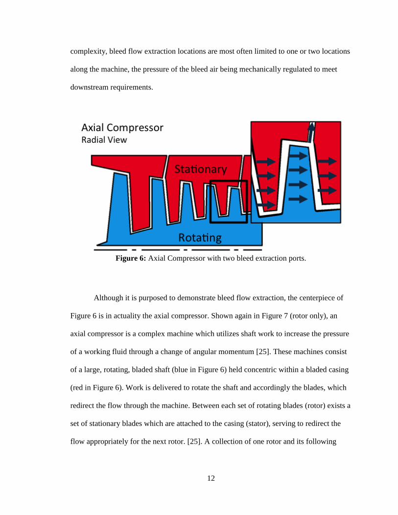
12

complexity, bleed flow extraction locations are most often limited to one or two locations

along the machine, the pressure of the bleed air being mechanically regulated to meet

downstream requirements.

Figure 6: Axial Compressor with two bleed extraction ports.

Although it is purposed to demonstrate bleed flow extraction, the centerpiece of

Figure 6 is in actuality the axial compressor. Shown again in Figure 7 (rotor only), an

axial compressor is a complex machine which utilizes shaft work to increase the pressure

of a working fluid through a change of angular momentum [25]. These machines consist

of a large, rotating, bladed shaft (blue in Figure 6) held concentric within a bladed casing

(red in Figure 6). Work is delivered to rotate the shaft and accordingly the blades, which

redirect the flow through the machine. Between each set of rotating blades (rotor) exists a

set of stationary blades which are attached to the casing (stator), serving to redirect the

flow appropriately for the next rotor. [25]. A collection of one rotor and its following

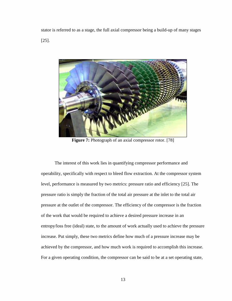
13

stator is referred to as a stage, the full axial compressor being a build-up of many stages

[25].

Figure 7: Photograph of an axial compressor rotor. [78]

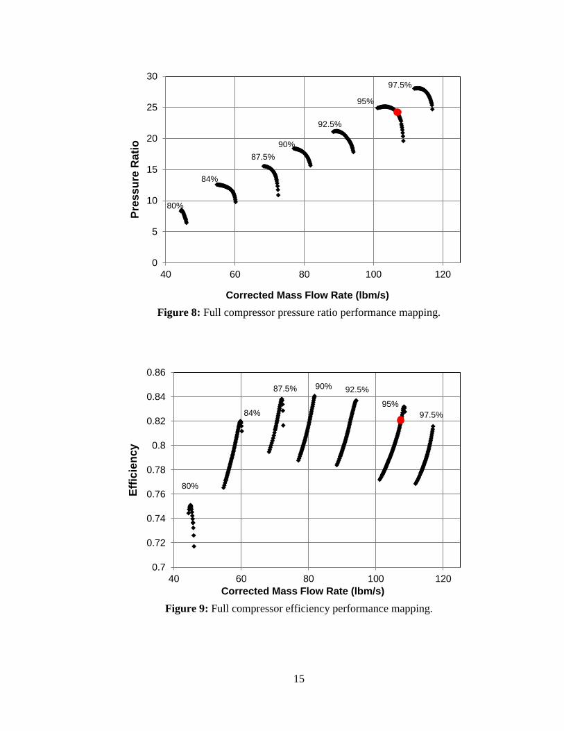
The interest of this work lies in quantifying compressor performance and

operability, specifically with respect to bleed flow extraction. At the compressor system

level, performance is measured by two metrics: pressure ratio and efficiency [25]. The

pressure ratio is simply the fraction of the total air pressure at the inlet to the total air

pressure at the outlet of the compressor. The efficiency of the compressor is the fraction

of the work that would be required to achieve a desired pressure increase in an

entropy/loss free (ideal) state, to the amount of work actually used to achieve the pressure

increase. Put simply, these two metrics define how much of a pressure increase may be

achieved by the compressor, and how much work is required to accomplish this increase.

For a given operating condition, the compressor can be said to be at a set operating state,

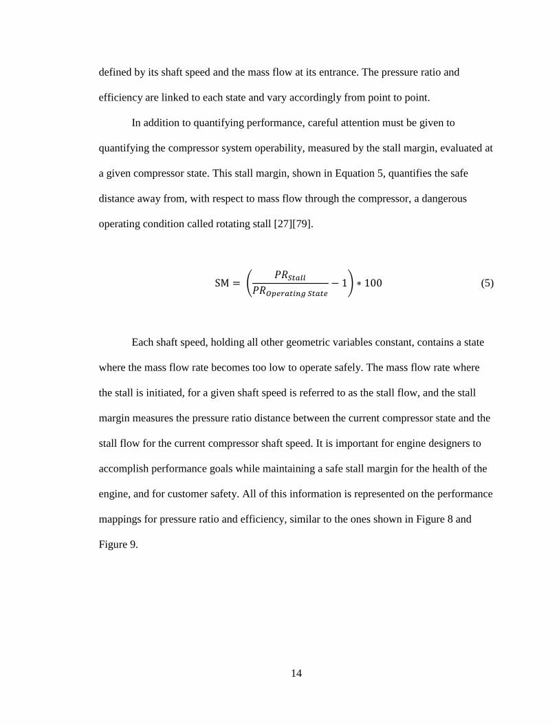
14

defined by its shaft speed and the mass flow at its entrance. The pressure ratio and

efficiency are linked to each state and vary accordingly from point to point.

In addition to quantifying performance, careful attention must be given to

quantifying the compressor system operability, measured by the stall margin, evaluated at

a given compressor state. This stall margin, shown in Equation 5, quantifies the safe

distance away from, with respect to mass flow through the compressor, a dangerous

operating condition called rotating stall [27][79].

SM = (

𝑃𝑅𝑆𝑡𝑎𝑙𝑙𝑃𝑅𝑂𝑝𝑒𝑟𝑎𝑡𝑖𝑛𝑔 𝑆𝑡𝑎𝑡𝑒

− 1) ∗ 100 (5)

Each shaft speed, holding all other geometric variables constant, contains a state

where the mass flow rate becomes too low to operate safely. The mass flow rate where

the stall is initiated, for a given shaft speed is referred to as the stall flow, and the stall

margin measures the pressure ratio distance between the current compressor state and the

stall flow for the current compressor shaft speed. It is important for engine designers to

accomplish performance goals while maintaining a safe stall margin for the health of the

engine, and for customer safety. All of this information is represented on the performance

mappings for pressure ratio and efficiency, similar to the ones shown in Figure 8 and

Figure 9.

15

Figure 8: Full compressor pressure ratio performance mapping.

Figure 9: Full compressor efficiency performance mapping.

0

5

10

15

20

25

30

40 60 80 100 120

Pre

ss

ure

Rati

o


0.7

0.72

0.74

0.76

0.78

0.8

0.82

0.84

0.86

40 60 80 100 120

Eff

icie

ncy


97.5%

97.5%

95%

95%

92.5%

92.5% 90%

90%

87.5%

87.5%

84%

84%

80%

80%

16

A compressor performance map allows one to quantify the pressure ratio,

efficiency, and stall margin of the compressor at any given operating state [22]. On a

performance map, a compressor state is defined by corrected parameters, namely

corrected mass flow at the compressor entrance and corrected shaft speed, shown in

Equation 6 and Equation 7, respectively. These corrected quantities are used to relate the

compressor operating conditions in the sea level static environment to those at all other

altitudes and temperatures [70]. Corrected quantities more appropriately capture

compressor performance and operability since the machine will experience a wide variety

of operating conditions not experienced during ground testing.

𝑊𝑐 = W ∗

√𝑇/𝑇𝑆𝑇𝐷𝑃/𝑃𝑆𝑇𝐷

(6)

𝑁𝐶 =

N

√𝑇/𝑇𝑆𝑇𝐷 (7)

The behavior of the compressor is captured in its performance map, and it is

useful to understand the general relationship between the compressor state points, or

movement from one state point to another on a compressor map, and the resultant

efficiency and pressure ratio. The compressor is designed and sized for a certain pressure

ratio and efficiency, accomplished at a specific corrected state, named the “on design”

operating state. Outside of the “on design” state, the efficiency will very often drop off

from its maximum [25]. Additionally, the shaft speed where the “on design” state is

operating will often contain the higher efficiency potential than all other speeds falling

17

short of this. However, with respect to pressure ratio, as the shaft speed increases, the

flow deflection through the compressor increases, causing an increase.

The relationship between mass flow and pressure ratio is slightly more complex.

At the lowest flow state of interest, near the stall flow, the compressor is achieving its

highest possible pressure ratio for a given shaft rotational speed. As the flow increases,

the operating point moves away from the stall flow, and reduces in pressure ratio, until a

state of choke is encountered. Choke is the point at which the mass flow through the

compressor is too high to effectively increase the pressure at the given shaft speed [49].

As an example, consider the red point on Figure 8 and Figure 9, which defines the

compressor operating state at a corrected mass flow rate of 107 {lbm/s} and a corrected

shaft speed of 95% of the design speed. At this point, it can be seen that the compressor is

achieving a pressure ratio of 24 and an efficiency of 82%. In addition, the compressor is

operating with a stall margin of 4.1%, as the pressure ratio at stall is equal to 25.

Aerodynamic Instability

The stall margin to this point has been used to define the pressure ratio difference

between the operating state and the point of stall. Stall is a phenomenon that occurs in

rotating compressors, where the mass flow across a blade is low enough to cause

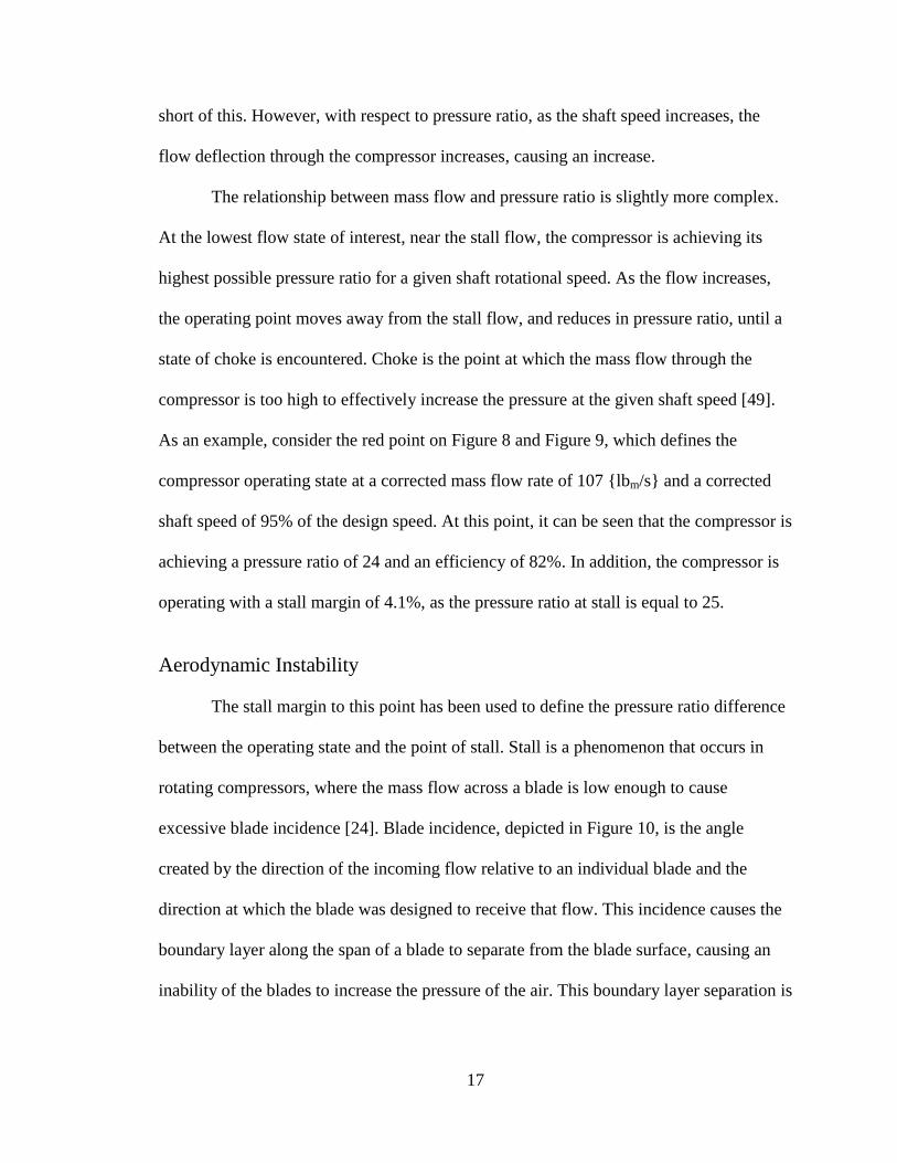
excessive blade incidence [24]. Blade incidence, depicted in Figure 10, is the angle

created by the direction of the incoming flow relative to an individual blade and the

direction at which the blade was designed to receive that flow. This incidence causes the

boundary layer along the span of a blade to separate from the blade surface, causing an

inability of the blades to increase the pressure of the air. This boundary layer separation is

18

the point at which the compressor is no longer properly performing, and is typically the

point at which a dangerous phenomenon called surge is initiated [24].

Figure 10: Initiation of boundary layer separation as mass flow is reduced.

As the flow through a compressor is reduced even further than the point of

boundary layer separation and the corresponding inability to increase the pressure,

explained before, the machine is left susceptible to violent flow reversal. This is due to

the compressor operating across an adverse pressure gradient, meaning the air pressure at

the outlet of any stage is higher than the air pressure at the inlet [27]. When the

pressurization of the air is suddenly halted inside the machine, the higher pressure air

reverses in the direction of the lower pressure air. This reversal in effect unloads the

compressor, allowing for the re-pressurization of the machine at the same mass flow as

before, causing the cycle to repeat violently until more mass flow is allowed through the

machine. A simple diagram of the flow separation along the blade suction surface is

shown in Figure 10, where the blades are experiencing various flow rates beginning with

the design flow on the left, and reducing to the initial stall flow on the right.

Design Flow Separation Begins Stall Occurs

Incidence = 4° Incidence = 0° Incidence = 8°

19

As discussed before, rotating stall is initiated by severely large amounts of blade

incidence, which in actuality is a consequence of operating the compressor at too low of a

mass flow rate. A natural aid in avoiding this issue is found in giving the

machine/operator the freedom to actively reduce the level of blade incidence [14]. This is

accomplished through the implementation of variable stator vanes (VSV) [64]. These are

blades, rotatable about each individual blade’s radial axis, which are fixed to the casing

(red in Figure 6), including inlet guide vanes (IGV) and stators. Controlled by actuators,

VSV blade rows operate at various angular settings throughout the compressor

operational envelope to maintain operability requirements while maximizing performance

potential [27]. Most compressor systems which employ VSVs do so by constraining the

motion of each blade row to the other rows, through a mechanical device. This means

that the rotated angles experienced by each row are not independent of the rotational

angle of the other rows, constraining the utilization of the VSVs to a set schedule, once

assembled.

Each of the features of an axial compressor, specifically bleed flow extraction and

VSV settings have an impact on the performance and operability of the machine [68]

[69]. This means that the performance map for any compressor is not only a function of

the fixed geometry of the machine, but also bleed flow rate, location, and VSV

orientation. A compressor map speed line is the collection of all the compressor operating

states for a fixed shaft speed between the stall flow and the choked flow. Inherent to each

speed line is the bleed flow rate and bleed flow location, as well as the orientation of each

VSV [49] [59]. The compressor map used to represent a full compressor operating

envelope is a collection of speed lines, each speed line representing only the performance

20

of the machine under one specific bleed and VSV setting [49] [59]. All of that to say, in

order to capture the performance impacts of bleed and VSV across a range of settings,

using traditional methods, it would require an individual map for each bleed and VSV

setting of interest, as any of these settings will produce a collection of speed lines, and

performance and operability metrics which are different for the same envelope of

operating states.

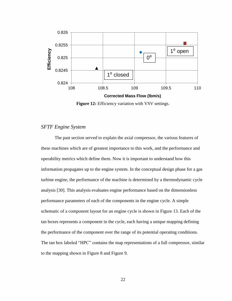
An example of this change may be seen in Figure 11 and Figure 12, where

speedlines have been constructed from the condition where the IGV is rotated to deflect

the flow one degree closed and then one degree open, offsetting the flow into the first

rotating stage of an axial compressor, while holding all of the other parameters constant.

Figure 9 shows only a slight variation in the IGV angle having a meaningful impact on

the pressure ratio at each state along the speed line. For example, if the compressor was

rotating at this speed, and at a flow rate of 107 {lbm/s}, and the IGV was rotated 1 degree

open or 1 degree closed, the pressure ratio achieved by this machine would drop from

26.5 to 25.7 or rise from 26.5 to 26.9 respectively, exhibiting a very high sensitivity to

this variation. As could be expected, these impacts are at least in part, due to the effects

this variation has on the efficiency of the compressor. Figure 10 shows the maximum

efficiency achieved by each speed line, and shows the same trend as before, where

slightly closing and opening the IGV largely impacted the system performance. This

parameter is scheduled specifically to a given compressor, and as such, this simple

example does not hold true for all compressors at all operating states.

The rotational orientation of the IGV, as well as all of the VSVs, does not only

impact the pressure ratio and efficiency of the compressor, but also affects its flow

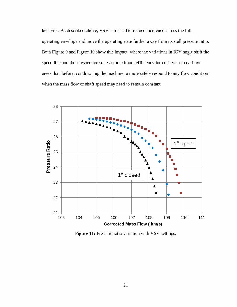
21

behavior. As described above, VSVs are used to reduce incidence across the full

operating envelope and move the operating state further away from its stall pressure ratio.

Both Figure 9 and Figure 10 show this impact, where the variations in IGV angle shift the

speed line and their respective states of maximum efficiency into different mass flow

areas than before, conditioning the machine to more safely respond to any flow condition

when the mass flow or shaft speed may need to remain constant.

Figure 11: Pressure ratio variation with VSV settings.

21

22

23

24

25

26

27

28

103 104 105 106 107 108 109 110 111

Pre

ss

ure

Rati

o

Corrected Mass Flow (lbm/s)

1⁰ open

1⁰ closed

22

Figure 12: Efficiency variation with VSV settings.

SFTF Engine System

The past section served to explain the axial compressor, the various features of

these machines which are of greatest importance to this work, and the performance and

operability metrics which define them. Now it is important to understand how this

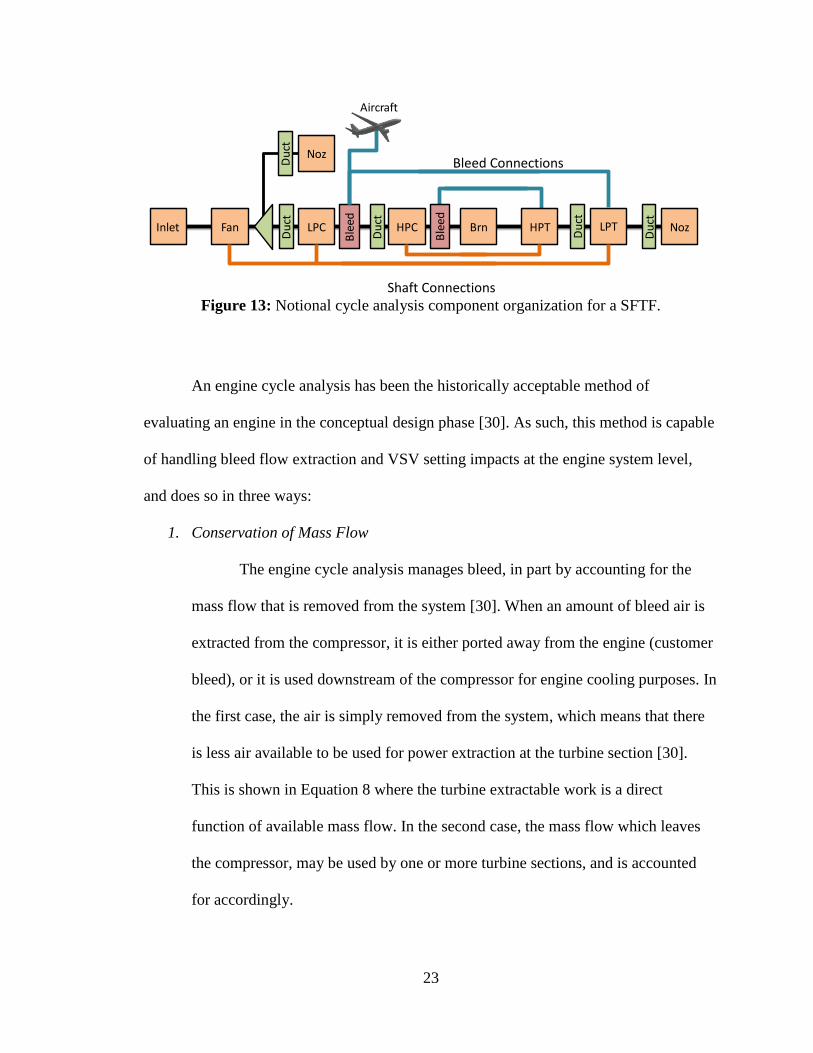
information propagates up to the engine system. In the conceptual design phase for a gas

turbine engine, the performance of the machine is determined by a thermodynamic cycle

analysis [30]. This analysis evaluates engine performance based on the dimensionless

performance parameters of each of the components in the engine cycle. A simple

schematic of a component layout for an engine cycle is shown in Figure 13. Each of the

tan boxes represents a component in the cycle, each having a unique mapping defining

the performance of the component over the range of its potential operating conditions.

The tan box labeled “HPC” contains the map representations of a full compressor, similar

to the mapping shown in Figure 8 and Figure 9.

0.824

0.8245

0.825

0.8255

0.826

108 108.5 109 109.5 110

Eff

icie

ncy


1⁰ closed

1⁰ open

0⁰

23

Figure 13: Notional cycle analysis component organization for a SFTF.

An engine cycle analysis has been the historically acceptable method of

evaluating an engine in the conceptual design phase [30]. As such, this method is capable

of handling bleed flow extraction and VSV setting impacts at the engine system level,

and does so in three ways:

1. Conservation of Mass Flow

The engine cycle analysis manages bleed, in part by accounting for the

mass flow that is removed from the system [30]. When an amount of bleed air is

extracted from the compressor, it is either ported away from the engine (customer

bleed), or it is used downstream of the compressor for engine cooling purposes. In

the first case, the air is simply removed from the system, which means that there

is less air available to be used for power extraction at the turbine section [30].

This is shown in Equation 8 where the turbine extractable work is a direct

function of available mass flow. In the second case, the mass flow which leaves

the compressor, may be used by one or more turbine sections, and is accounted

for accordingly.

Inlet Fan LPC

Ble

ed HPC

Ble

ed

Brn HPT LPT Noz

Noz

Du

ct

Du

ct

Du

ct

Du

ct

Du

ct

Aircraft

Bleed Connections

Shaft Connections

24

𝑇𝑢𝑟𝑏𝑖𝑛𝑒 𝑊𝑜𝑟𝑘 = 𝑊 ∗ (∆𝐻𝑇𝑢𝑟𝑏𝑖𝑛𝑒) (8)

2. Balance of Work

Bleed flow extraction is also managed by means of the work balance

maintained throughout the engine [30]. In the case where the bleed air is ported

away from the engine for customer use, there is an amount of work that must be

expended by the compressor to simply prepare it for the customer. This wasted

work must be provided by the turbine section and will require a greater amount of

fuel burned by the engine. This relationship is shown in Equation 9. Bleed air

which is returned downstream of the compressor will also impact the cycle

performance, as it requires work to achieve a certain pressure, but can later

contribute to the cycle performance by means of non-chargeable cooling, and

active clearance control.

𝑇𝑢𝑟𝑏𝑖𝑛𝑒 𝑊𝑜𝑟𝑘 = 𝐶𝑜𝑚𝑝𝑟𝑒𝑠𝑠𝑜𝑟 𝑊𝑜𝑟𝑘 + 𝐵𝑙𝑒𝑒𝑑 𝐴𝑖𝑟 𝑊𝑜𝑟𝑘 (9)

3. Utilization of Component Maps

The final method that the cycle analysis utilizes for handling bleed flow

extraction and VSV settings is through the proper management of the compressor

performance map [69]. As explained before, the compressor performance map is

unique for any bleed flow and VSV setting. The cycle analysis includes this map,

and given that the analysis is being performed with the same bleed and VSV

settings as were used to construct the compressor performance map, this will

25

provide acceptable results [49]. That being said, any variations in bleed or VSV

setting will require the addition of a map constructed under the new bleed and

VSV setting in order to maintain the same level of uncertainty.

Regardless of whether or not the cycle analysis includes a map for every

configuration (bleed and VSV setting), the engine operating point will shift on the map

from the operating point before changing the configuration, to the point after the change

[27]. This is because the bleed handling methods discussed above require the cycle

analysis to rebalance as the work and mass conservation account for the bleed. An

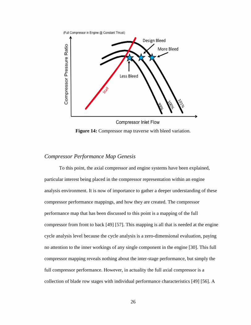
example of this is shown in Figure 14, where the engine customer bleed is perturbed from

a baseline value at a constant thrust condition. This engine was sized for the customer

bleed at the baseline condition. It can be seen here that for a given bleed location and

VSV setting, increasing bleed flow rate will move the compressor away from stall, while

reducing this flow rate will bring the engine closer to stall. This behavior is utilized by

engine operators during the engine startup, where large amounts of air are bled off in

order to maintain a safe stall margin [27].

26

Figure 14: Compressor map traverse with bleed variation.

Compressor Performance Map Genesis

To this point, the axial compressor and engine systems have been explained,

particular interest being placed in the compressor representation within an engine

analysis environment. It is now of importance to gather a deeper understanding of these

compressor performance mappings, and how they are created. The compressor

performance map that has been discussed to this point is a mapping of the full

compressor from front to back [49] [57]. This mapping is all that is needed at the engine

cycle analysis level because the cycle analysis is a zero-dimensional evaluation, paying

no attention to the inner workings of any single component in the engine [30]. This full

compressor mapping reveals nothing about the inter-stage performance, but simply the

full compressor performance. However, in actuality the full axial compressor is a

collection of blade row stages with individual performance characteristics [49] [56]. A

27

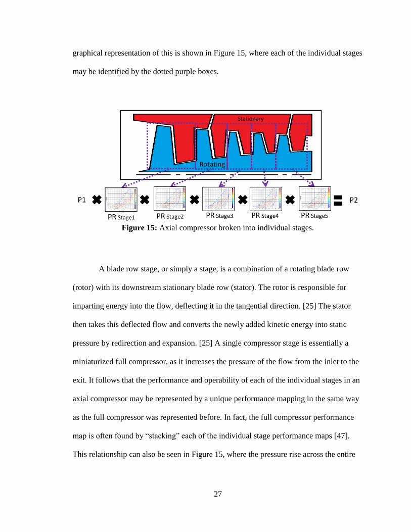
graphical representation of this is shown in Figure 15, where each of the individual stages

may be identified by the dotted purple boxes.

Figure 15: Axial compressor broken into individual stages.

A blade row stage, or simply a stage, is a combination of a rotating blade row

(rotor) with its downstream stationary blade row (stator). The rotor is responsible for

imparting energy into the flow, deflecting it in the tangential direction. [25] The stator

then takes this deflected flow and converts the newly added kinetic energy into static

pressure by redirection and expansion. [25] A single compressor stage is essentially a

miniaturized full compressor, as it increases the pressure of the flow from the inlet to the

exit. It follows that the performance and operability of each of the individual stages in an

axial compressor may be represented by a unique performance mapping in the same way

as the full compressor was represented before. In fact, the full compressor performance

map is often found by “stacking” each of the individual stage performance maps [47].

This relationship can also be seen in Figure 15, where the pressure rise across the entire

P1 P2

PR Stage1 PR Stage2 PR Stage3 PR Stage4 PR Stage5

Stationary

Rotating

28

machine is found by multiplying the pressure ratio across each of the subsequent stages

[47].

There are many ways to create full compressor mappings, the differences lying in

the desired fidelity, time and cost available, and knowledge about the final design [13].

Broadly speaking, compressor maps can be created from the following methods, starting

at the lowest fidelity and working up: (It must be noted that many other methods of

varying fidelity exist, not explained here.)

1. 1D Meanline Analysis

The meanline analysis is often the first step in the compressor design process,

allowing the engineer to find a first approximation of the compressor’s geometry

and subsequent performance mapping [44]. Stage by stage flow characteristics are

found based on the fundamental aerodynamics and thermodynamics behind these

devices [67]. A meanline analysis is the tool used by compressor designers in the

conceptual design phase, because very little is known about the final design aside

from the intended performance [66]. This analysis may be performed strictly

across the mean radial line of each compressor row, or may be applied in the same

way across multiple radial sections of the machine (multi-stream meanline).

Utilizing a multi-stream meanline approach allows one to more fully characterize

the radial flow profile throughout the machine without sacrificing the speed and

computational cost savings that are forfeited with greater fidelity analyses.

29

2. 2D Streamline Curvature

The streamline curvature (SLC) or more generally, all two dimensional

turbomachinery analyses evaluate the compressor performance based on an

approach which uses a large number of streamlines [44]. SLC analyses take into

account actual airfoil data with respect to the blade, revealing information about

flow behavior at the blade edges [44]. This differs from the multi-stream meanline

analysis from before in the particular attention to the lift generation and spanwise

pressure distribution across the full blade surface which was previously neglected

[73]. This analysis requires more knowledge about the final design than what is

usually available in the conceptual design phase.

3. 3D Computational Fluid Dynamics

An even higher fidelity available to compressor designers currently stands as the

state of the art in computer aided design: Computational fluid dynamics (CFD)

[19]. CFD is used to simulate the full three dimensional environment inside of an

axial compressor, attempting to handle complex flow behavior between blades

and blade rows at a large number of radial positions along each blade. [19] This is

a computationally effort and time expensive activity that requires nearly full

knowledge about the geometry of the final compressor design, which is certainly

not available in the conceptual design phase. [13]

30

4. Full Compressor Experimental Rig Test

The highest fidelity available for constructing a full compressor performance map

is found by means of an experimental rig test. In a rig test, the full compressor is

physically produced and placed on a test stand. Driven by a motor or turbine, the

compressor is operated to a set speed under a choked condition (full mass flow)

[65]. Data is collected at this point before closing a throttling valve, often located

downstream of the compressor exit, in order to decrease the mass flow through

the machine. This is continued, all the while collecting data, until the compressor

approaches stall, at which point the flow is opened back up to full, and the process

is repeated for another rotational speed. [65] This allows for the full

characterization of the compressor performance within its expected operating

range.

Research Questions

The central aim of this work is to develop the ability to, in the conceptual design

phase, determine the minimum engine core size to meet compressor performance and

operability while accounting for subsystem bleed requirements. Traditional gas turbine

cycle analysis methodology has delivered the ability to account for customer subsystem

bleed requirements at the engine level, but either neglects the compressor level impacts of

this bleed extraction, or requires an individual compressor map for every bleed

configuration of interest, making design space exploration difficult. Therefore, there is a

need to develop a modeling approach to account for bleed flow extraction in the context

of an engine cycle design, with particular intention to capturing the compressor level

31

impacts in an engine level environment. In order to accomplish this, the following

research questions must be answered:

1. How can the compressor level impacts be sufficiently captured using a meanline

analysis, and how big of an impact exists?

As explained before, in the conceptual design phase of an axial

compressor, meanline analyses are utilized to establish the initial geometry and

system configuration. In order to capture the impact of bleed at the compressor

level, a multi-stream meanline analysis will be applied to estimate the individual

performance of each stage. Once all of the individual stage performance mappings

are created, a stage stacking method will be utilized to construct a full compressor

performance map, combining the performance of each of its individual stages.

Bleed flow extraction may then be accounted for by drawing the desired amount

of flow out of the compressor at any inter-stage location and flow rate. This will

reduce the flow into the downstream stages, impacting only the operating point

and incoming flow conditions of each. By accounting for bleed in this way, the

physics behind the full compressor are maintained while the individual stage

performance maps are unaffected by the bleed flow extraction.

Once this modeling method is implemented it may be utilized to quantify

the impacts of varying bleed flow rate and bleed flow location on the full

performance map. In addition, this modeling environment will need to be able to

capture the impacts of each VSV setting on the full performance map, since these

two features interact to maintain operability and performance [27] [66]. Each of

32

the variables above will impact the full compressor pressure ratio, efficiency, and

stall flow, across the entire range of operating conditions.

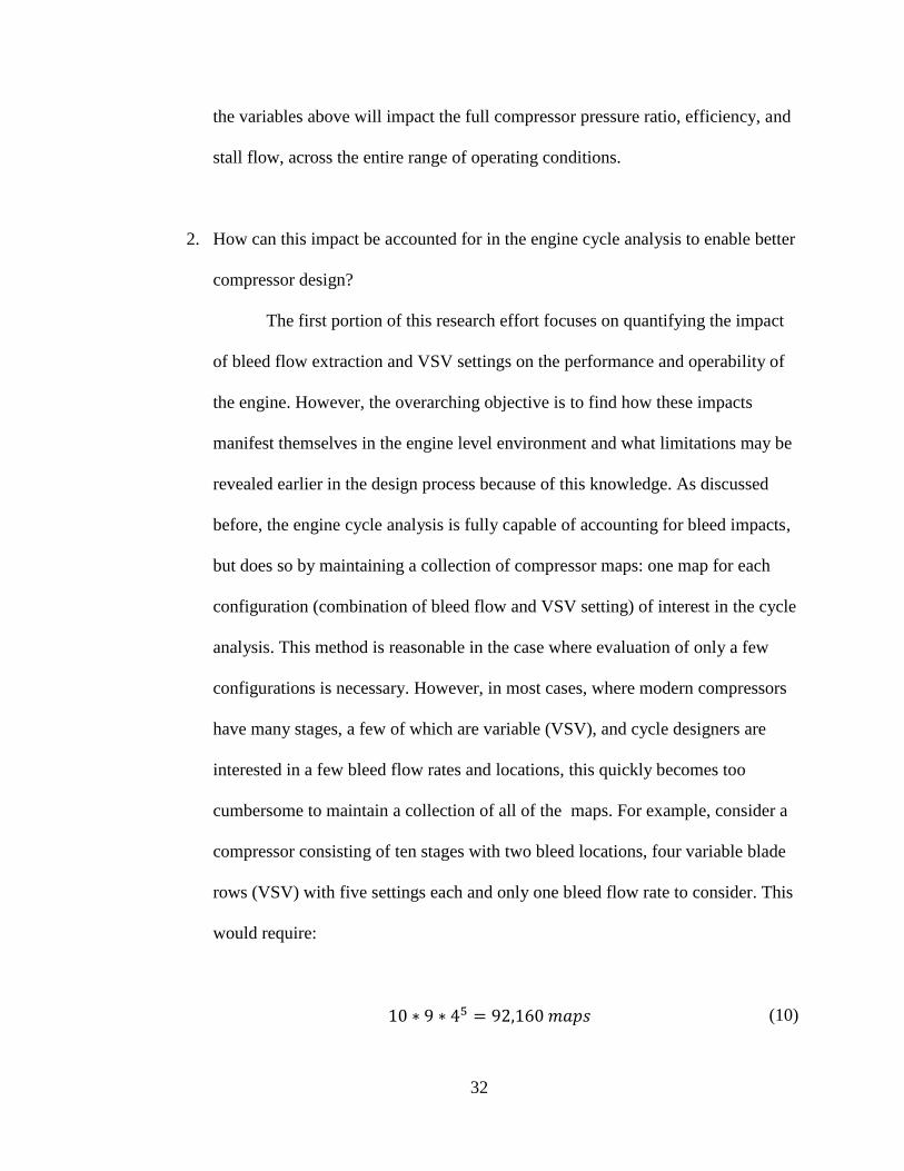
2. How can this impact be accounted for in the engine cycle analysis to enable better

compressor design?

The first portion of this research effort focuses on quantifying the impact

of bleed flow extraction and VSV settings on the performance and operability of

the engine. However, the overarching objective is to find how these impacts

manifest themselves in the engine level environment and what limitations may be

revealed earlier in the design process because of this knowledge. As discussed

before, the engine cycle analysis is fully capable of accounting for bleed impacts,

but does so by maintaining a collection of compressor maps: one map for each

configuration (combination of bleed flow and VSV setting) of interest in the cycle

analysis. This method is reasonable in the case where evaluation of only a few

configurations is necessary. However, in most cases, where modern compressors

have many stages, a few of which are variable (VSV), and cycle designers are

interested in a few bleed flow rates and locations, this quickly becomes too

cumbersome to maintain a collection of all of the maps. For example, consider a

compressor consisting of ten stages with two bleed locations, four variable blade

rows (VSV) with five settings each and only one bleed flow rate to consider. This

would require:

10 ∗ 9 ∗ 45 = 92,160 𝑚𝑎𝑝𝑠 (10)

33

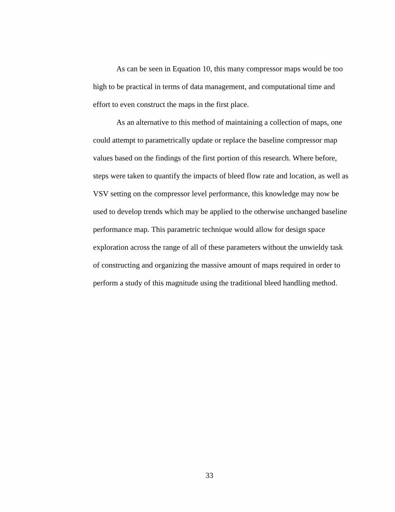
As can be seen in Equation 10, this many compressor maps would be too

high to be practical in terms of data management, and computational time and

effort to even construct the maps in the first place.

As an alternative to this method of maintaining a collection of maps, one

could attempt to parametrically update or replace the baseline compressor map

values based on the findings of the first portion of this research. Where before,

steps were taken to quantify the impacts of bleed flow rate and location, as well as

VSV setting on the compressor level performance, this knowledge may now be

used to develop trends which may be applied to the otherwise unchanged baseline

performance map. This parametric technique would allow for design space

exploration across the range of all of these parameters without the unwieldy task

of constructing and organizing the massive amount of maps required in order to

perform a study of this magnitude using the traditional bleed handling method.

34

CHAPTER III: METHODOLOGY

With the goal of developing a modeling approach to account for bleed flow

extraction in the context of both compressor and engine cycle design, with particular

intention to capturing the compressor level impacts, two central tasks have emerged:

1) Sufficiently capture and quantify the compressor level impacts, using a multi-

stream, meanline analysis.

2) Account for these impacts in the engine cycle analysis to enable better compressor

design by analysis of the compressor’s operating line, stall margin, and engine

TSFC.

Upon successful completion of these tasks, a compressor designer should be equipped

with the knowledge and tools necessary to be able to determine the minimum engine core

size to meet compressor performance and operability, given the customer bleed flow

extraction requirements.

Experiment 1

The first task requires capturing the performance and operability impacts of bleed

flow extraction at the compressor level. As discussed before, bleed flow extraction and

VSVs are often utilized simultaneously and their impacts are coupled, especially with

respect to compressor operability. [27] For that reason, special care will be taken to first

model the impacts of VSV settings at the compressor level.

Modeling the impact of VSVs, using a meanline analysis requires only a slight

change to what would be required to model a compressor without VSVs. To understand

35

this change, one must first understand how a compressor physically works to increase the

pressure of a fluid. Figure 16 shows the velocity triangles for a single compressor stage.

The flow enters the compressor at the absolute inlet flow angle 𝛼1, having been oriented

in this direction from the upstream stage or an IGV. The rotor deflects this flow further,

which departs the blade row at the new absolute flow angle 𝛼2 before entering the stator.

The stator then deflects the flow back a certain amount, repositioning it for the next stage.

Since the rotor is traveling through space, it receives and releases the flow at relative flow

angles, 𝛽1 and 𝛽2. For this reason, the actual blade metal angles for the rotor are

constructed to match these relative flow angles, with the assumption that no incidence is

experienced at the design condition. The stator blades are not moving, and as such are

designed with their physical blade metal angles equivalent to the absolute flow angles

experienced, with the same assumption of zero incidence as before, at the on-design

condition. In addition to this, both the rotor and stator blades are designed with a certain

“stagger angle” which is simply the angle between the blade chord (line connecting blade

leading edge tip to trailing edge tip) and the axial direction. In order to model VSV

orientation, one can simply vary the stagger angle of any variable stator blade row in the

machine.

36

Figure 16: Flow deflection through a single compressor stage.

The Object-oriented Turbomachinery Analysis Code (OTAC) is a turbomachinery

meanline analysis, modeling environment used by the Aerospace Systems Design

Laboratory (ASDL) which takes a given compressor geometry, mass flow, and shaft

speed characteristic, and estimates the compressor performance. [71] This code is used to

produce a performance map, created from first evaluating the performance of each stage

in the compressor and then stacking these stages to evaluate the total compressor

performance. OTAC is capable of implementing shock, profile, and end wall loss models,

detecting stall, predicting incidence and deviation, and implementing viscous blockage

effects. OTAC also has the ability to incorporate a meanline analysis across multiple

𝐶𝑦

𝛼3

Stator

Blade Row

𝐶𝑥

𝛼1 𝛽1 Stage

Entrance

Rotor

Blade Row

𝑊1

𝛽2 𝐶2 𝛼2

𝐶𝑥 𝑊2

U

U

Stage Exit 𝐶𝑥

𝐶1

37

streamlines, varying radially and allowing for a more two dimensional analysis with

similar computational load to that of what would be expected of a one dimensional

meanline analysis.

As stated before, VSV impacts will be incorporated into the compressor modeling

environment by updating the individual variable blade row’s inlet and outlet blade angles,

equivalent to updating the blade stagger angle, allowing for less incidence to occur at off-

design conditions. The model will be evaluated using the NASA E3 compressor, which

was part of one of the largest aeronautical research and development programs in history,

where NASA aimed to develop technologies necessary to achieve greater fuel efficiency

for future gas turbine engines [64]. The E3, shown in Figure 17, is a ten stage compressor,

utilizing six rows of VSVs, and in its completed form allows for bleed flow extraction at

two axial locations.

Figure 17: Radial cross section of the full E

3 compressor.

The E3 compressor was tested in two phases of interest. The “Build 1” (B1)

testing was conducted upon the compressor with the first set of bladeing, the VSV setting

schedule shown in Figure 18, and no bleed flow extraction applied. [64] Testing was

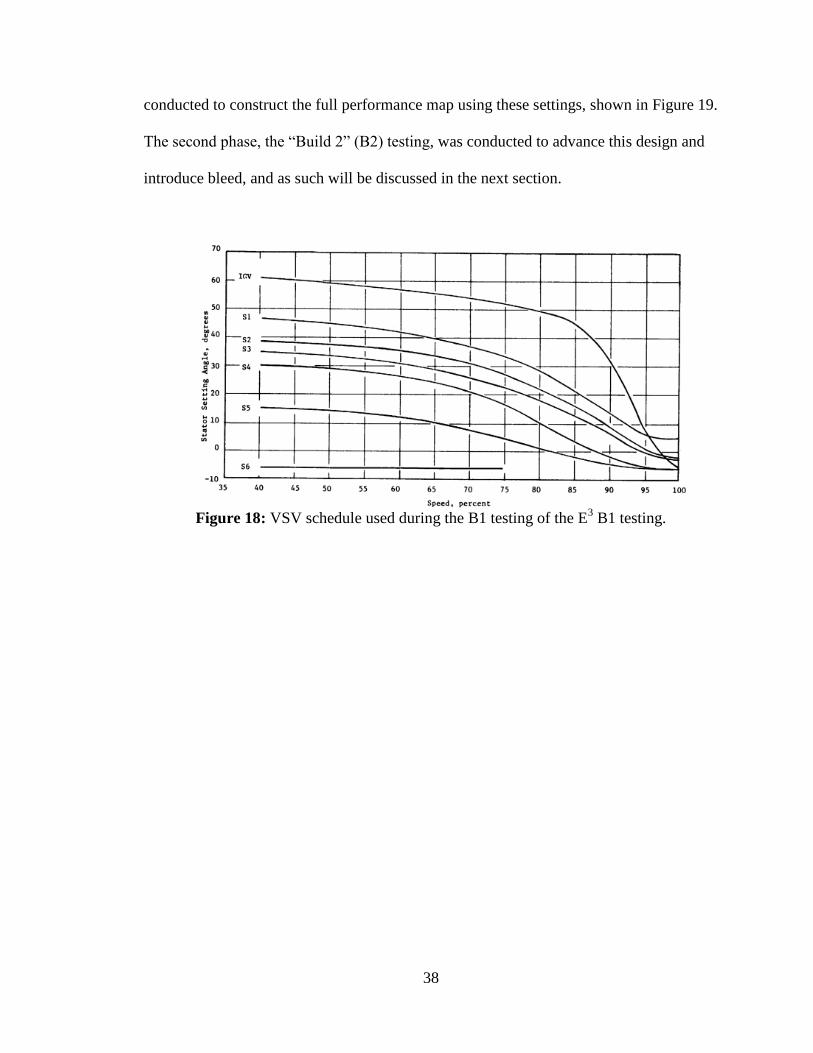
38

conducted to construct the full performance map using these settings, shown in Figure 19.

The second phase, the “Build 2” (B2) testing, was conducted to advance this design and

introduce bleed, and as such will be discussed in the next section.

Figure 18: VSV schedule used during the B1 testing of the E

3 B1 testing.

39

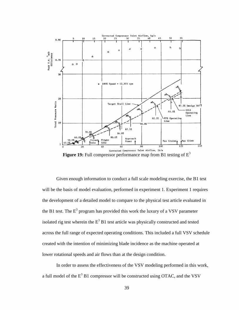
Figure 19: Full compressor performance map from B1 testing of E

3

Given enough information to conduct a full scale modeling exercise, the B1 test

will be the basis of model evaluation, performed in experiment 1. Experiment 1 requires

the development of a detailed model to compare to the physical test article evaluated in

the B1 test. The E3 program has provided this work the luxury of a VSV parameter

isolated rig test wherein the E3 B1 test article was physically constructed and tested

across the full range of expected operating conditions. This included a full VSV schedule

created with the intention of minimizing blade incidence as the machine operated at

lower rotational speeds and air flows than at the design condition.

In order to assess the effectiveness of the VSV modeling performed in this work,

a full model of the E3 B1 compressor will be constructed using OTAC, and the VSV

40

schedule will be varied to explore the impact of this on the compressor’s operating range.

The model will first be performed using the design speed (100%) VSV angles for the

compressor speeds most nearly matching the maximum climb (97.5%), maximum cruise

(95%), and approach (90%) engine flight conditions. This will establish the baseline,

representing an engine with a fixed operating range, constrained to excessive incidence as

the compressor operates further away from design. Following this, the model will be

operated with the VSV orientations set to the prescribed operating schedule for the E3 B1

rig testing. To this point, it is expected that the second performance mapping will closely

match the empirical test data, with respect to the useful operating range of each of the

speedlines, where in the first mapping this should not be the case.

To further assess the effectiveness of the VSV modeling performed here, the

model will be operated once more, but with the VSVs opened, and then closed an

additional 10% of their effective range at each speedline discussed above. The VSVs are

modeled to be adjustable by a percentage of their useful range, because the relationship

between these VSVs and the rest of the machine is unique, and there is a rotational

constraint between each VSV and the rest of the VSVs. Additionally, this mirrors the

behavior of a physical compressor, which often uses a single shaft driven by a single

actuator, which is mechanically constrained to the VSVs through proportional

transmission. The trends of this final testing will be compared to the NACA 8 stage

compressor program, which analyzed similar impacts.

41

Experiment 2

The first experiment will be conducted with the intention of isolating the impacts

of VSVs within the modeling environment, and also serves to establish the baseline

model with respect to a compressor of the E3

performance and operating range. By

isolating the impacts of VSVs, the previous testing will enable the opportunity for better

isolation of the bleed flow extraction impacts for subsequent evaluations. The final step

in developing the capability to evaluate the impact of bleed flow extraction, coupled with

VSV utilization, on the compressor system is the integration of the bleed flow extraction

modeling, based on the physics of the process.

Explained before, the full axial compressor is in actuality a collection of many

single stage compressors stacked one after the other. [49] It is also true that the

performance and operability of each of these single stages can be represented by a single

stage performance map, similar to that of a full compressor. This fact may be utilized in

the modeling approach for bleed flow extraction in the following way:

1. Each stage will be characterized by an individual stage performance map.

2. Flow will then be extracted from the stations between any two compressors.

3. The individual stage maps will then be used in a stage stacking process to find the

full compressor performance mapping by combining the individual stage

performances, accounting for the flow condition into each individual stage.

This method isolates the bleed flow extraction to impact only the boundary conditions

entering the stages downstream of the bleed extraction location. It also creates

independence for the individual stage mappings, impacting only the individual stage

operating conditions and the full compressor performance mapping. Figure 20 and Figure

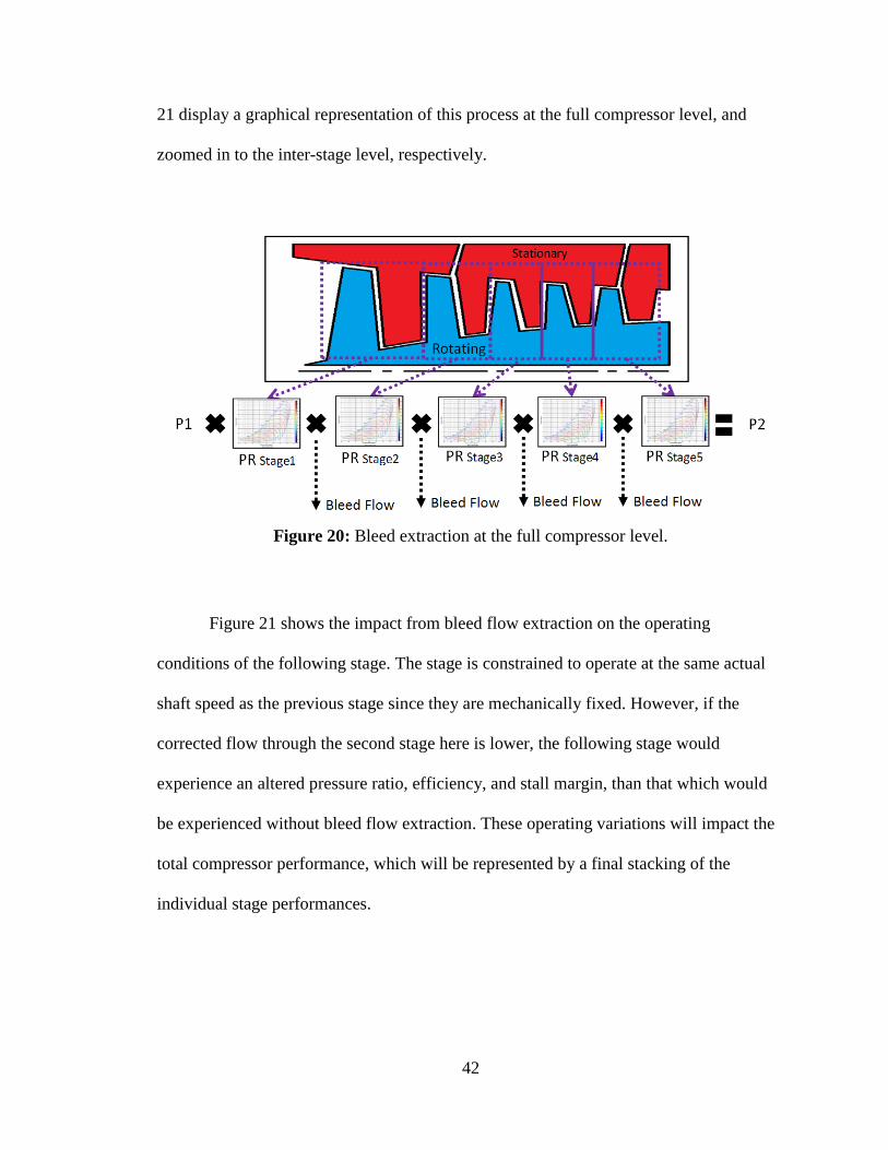
42

21 display a graphical representation of this process at the full compressor level, and

zoomed in to the inter-stage level, respectively.

Figure 20: Bleed extraction at the full compressor level.

Figure 21 shows the impact from bleed flow extraction on the operating

conditions of the following stage. The stage is constrained to operate at the same actual

shaft speed as the previous stage since they are mechanically fixed. However, if the

corrected flow through the second stage here is lower, the following stage would

experience an altered pressure ratio, efficiency, and stall margin, than that which would

be experienced without bleed flow extraction. These operating variations will impact the

total compressor performance, which will be represented by a final stacking of the

individual stage performances.

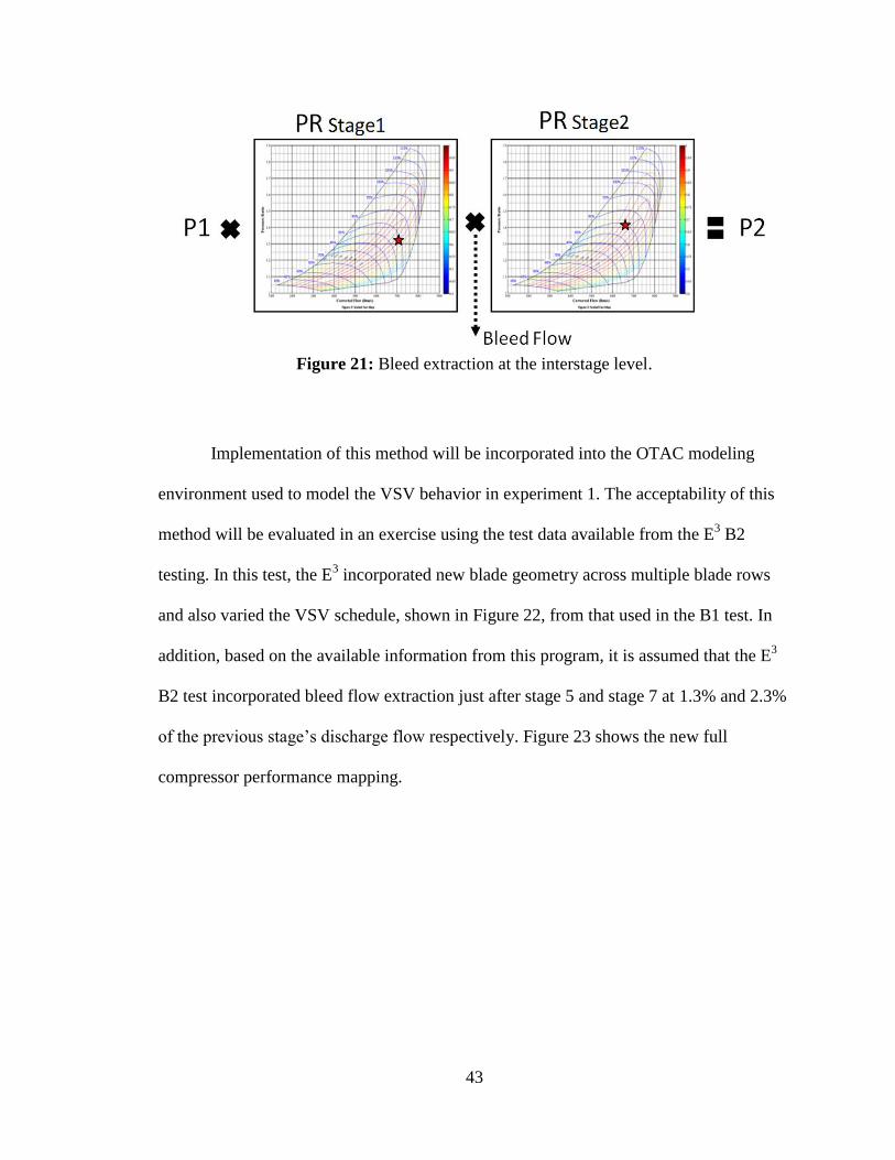
43

Figure 21: Bleed extraction at the interstage level.

Implementation of this method will be incorporated into the OTAC modeling

environment used to model the VSV behavior in experiment 1. The acceptability of this

method will be evaluated in an exercise using the test data available from the E3 B2

testing. In this test, the E3 incorporated new blade geometry across multiple blade rows

and also varied the VSV schedule, shown in Figure 22, from that used in the B1 test. In

addition, based on the available information from this program, it is assumed that the E3

B2 test incorporated bleed flow extraction just after stage 5 and stage 7 at 1.3% and 2.3%

of the previous stage’s discharge flow respectively. Figure 23 shows the new full

compressor performance mapping.

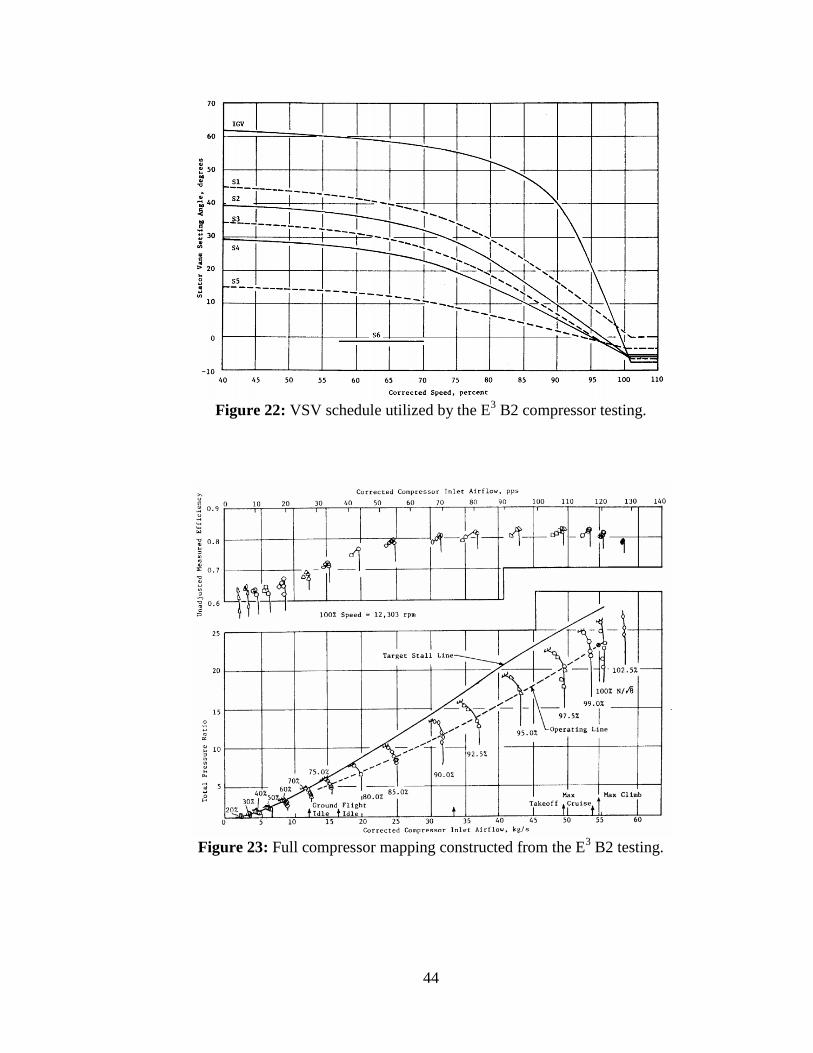
44

Figure 22: VSV schedule utilized by the E

3 B2 compressor testing.

Figure 23: Full compressor mapping constructed from the E

3 B2 testing.

45

Given enough information to conduct a full scale modeling exercise, the B2 test

will be the basis of model comparison performed in experiment 2. Experiment 2 requires

the extension of the OTAC model, evaluated in experiment 1, to compare with the

physical test article used in the B2 test. In order to perform this test, the full E3 B1

compressor, constructed in the OTAC modeling environment for experiment 1, will be

amended to include the addition of the bleed flow extraction model. The model will first

be operated without any bleed flow extraction, but including the VSV schedule

developed for the B1 experimental testing. This will establish the baseline, representing

an engine with variable geometry but without the capability for bleed flow extraction.

Following this, the model will be operated with the same VSV schedule as in the

first condition, but with the addition of the design bleed, with 1.3% and 2.3% of the

previous stage’s discharge flow being extracted at a location aft of the fifth and seventh

stages, respectively. This operating case represents the full variable geometry compressor

with the capability to include bleed flow extraction from either or both of the two

locations along the axial length of the compressor. It will be possible to qualify the

effectiveness of the bleed flow modeling based on the performance reduction found

between the E3 B1 and B2 full compressor experimental testing.

This exercise is subject to error from the blade geometry and VSV changes which

disallow the ability to isolate the bleed impacts alone. Additionally, the expected

remaining uncertainty from the first experiment, the change in bladeing, and the addition

of the bleed flow extraction, prevent the bleed modeling from being compared on a single

variable isolation basis. For this reason, the E3

B1 model should sufficiently capture the

trends that are expected, but will not be able to be calibrated against the empirical test

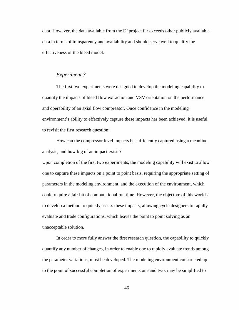
46

data. However, the data available from the E3 project far exceeds other publicly available

data in terms of transparency and availability and should serve well to qualify the

effectiveness of the bleed model.

Experiment 3

The first two experiments were designed to develop the modeling capability to

quantify the impacts of bleed flow extraction and VSV orientation on the performance

and operability of an axial flow compressor. Once confidence in the modeling

environment’s ability to effectively capture these impacts has been achieved, it is useful

to revisit the first research question:

How can the compressor level impacts be sufficiently captured using a meanline


Upon completion of the first two experiments, the modeling capability will exist to allow

one to capture these impacts on a point to point basis, requiring the appropriate setting of

parameters in the modeling environment, and the execution of the environment, which

could require a fair bit of computational run time. However, the objective of this work is

to develop a method to quickly assess these impacts, allowing cycle designers to rapidly

evaluate and trade configurations, which leaves the point to point solving as an

unacceptable solution.

In order to more fully answer the first research question, the capability to quickly

quantify any number of changes, in order to enable one to rapidly evaluate trends among

the parameter variations, must be developed. The modeling environment constructed up

to the point of successful completion of experiments one and two, may be simplified to

47

the form of Equation 11. This equation isolates the variables of interest to this work,

establishing the parametric definition of this modeling environment.

𝑃𝑅, 𝐸𝑓𝑓𝑖𝑐𝑖𝑒𝑛𝑐𝑦, 𝑆𝑡𝑎𝑙𝑙 𝐹𝑙𝑜𝑤 = 𝑓(𝑋1…𝑋5)

𝑋1 = 𝐶𝑜𝑟𝑟𝑒𝑐𝑡𝑒𝑑 𝑀𝑎𝑠𝑠 𝐹𝑙𝑜𝑤

𝑋2 = 𝐶𝑜𝑟𝑟𝑒𝑐𝑡𝑒𝑑 𝑆ℎ𝑎𝑓𝑡 𝑆𝑝𝑒𝑒𝑑

𝑋3 = 𝐵𝑙𝑒𝑒𝑑 𝐹𝑙𝑜𝑤 𝐿𝑜𝑐𝑎𝑡𝑖𝑜𝑛

𝑋4 = 𝐵𝑙𝑒𝑒𝑑 𝐹𝑙𝑜𝑤 𝑅𝑎𝑡𝑒

𝑋5 = 𝑉𝑆𝑉 𝑂𝑟𝑖𝑒𝑛𝑡𝑎𝑡𝑖𝑜𝑛𝑠

(11)

In order to evaluate trends among the parametric variations, a fairly encompassing

design space exploration is required. This may be accomplished through a design of

experiments (DoE) procedure which systematically varies the parameters of the

compressor model across a wide range of experiments. This allows for the design space

to be explored based on the design requirements and specific details of any given system.

In the case of the axial compressor model used in this work, one is interested in the

variation of these parameters across the entire design space, and particularly at the

extremes of the design space as the engine core size gets smaller. There are a variety of

DoE designs available to meet these requirements, two promising options including a

face centered, central composite design (FCCCD) and a Latin hypercube design. (LHD)

A face centered, central composite design (FCCCD) would allow for coverage of

the extremes of the design space, which would minimize the need for the model to

extrapolate responses. This would be ideal for the purposes of this work, but

unfortunately the modeling environment has exhibited poor convergence behavior at the

most extreme design space conditions in past work, which presents the potential issue of

48

the same happening here. The OTAC modeling environment used here exhibits poor

convergence behavior under extreme conditions, in large part due to the manual nature of

the flow initialization during each experiment. The model requires an initial estimate of

the starting flow, stall flow, and choke flow. An incorrect estimation of the starting flow

will yield an unconverged solution. On the other hand, an incorrect estimation of the stall

and choke flows yields either an overly bounded compressor line, limiting the availability

of valuable information, or causes the model to crash. As these effects have shown

themselves to be most aggressive at the extremes of the design space, the more

conservative, Latin hypercube design (LHD) will be used.

The LHD is a space filling design, which balances maximum spacing and

uniformity [45]. The LHD achieves a high level of accuracy in the interior of the design

space and is considered a robust DoE selection, managing most design spaces well. The

downside of this DoE, is that it achieves poor coverage at the corners of the design space,

although, for the purposes of this work, the LHD should be sufficient [45]. In order to

cover the design space using the LHD, each parameter will need to be able to be varied

by their individual resolutions, displayed in Table 1.

Table 1: Parameter variation for design of experiments

Variable Units Low High Resolution

Mass Flow (lbm/s) 30 140 0.1

Shaft Speed (% Design Speed) 80 100 2.5

VSV (Percent Open) -50 150 0.1

Bleed Rate (B5) (% Stage Incoming W) 1.3 10.3 0.1

Bleed Rate (B7) (% Stage Incoming W) 2.3 11.3 0.1

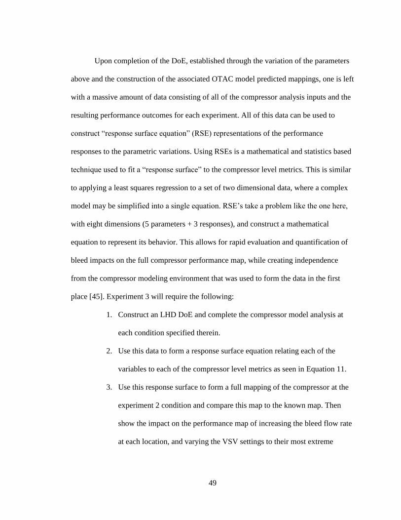
49

Upon completion of the DoE, established through the variation of the parameters

above and the construction of the associated OTAC model predicted mappings, one is left

with a massive amount of data consisting of all of the compressor analysis inputs and the

resulting performance outcomes for each experiment. All of this data can be used to

construct “response surface equation” (RSE) representations of the performance

responses to the parametric variations. Using RSEs is a mathematical and statistics based

technique used to fit a “response surface” to the compressor level metrics. This is similar

to applying a least squares regression to a set of two dimensional data, where a complex

model may be simplified into a single equation. RSE’s take a problem like the one here,

with eight dimensions (5 parameters + 3 responses), and construct a mathematical

equation to represent its behavior. This allows for rapid evaluation and quantification of

bleed impacts on the full compressor performance map, while creating independence

from the compressor modeling environment that was used to form the data in the first

place [45]. Experiment 3 will require the following:

1. Construct an LHD DoE and complete the compressor model analysis at

each condition specified therein.

2. Use this data to form a response surface equation relating each of the

variables to each of the compressor level metrics as seen in Equation 11.

3. Use this response surface to form a full mapping of the compressor at the

experiment 2 condition and compare this map to the known map. Then

show the impact on the performance map of increasing the bleed flow rate

at each location, and varying the VSV settings to their most extreme

50

conditions to assess the RSE’s ability to properly predict the expected

trends.

The final step functions as a use case to evaluate the effectiveness of the

capability developed in the first two steps. This simulates the use of the developed

capability in its intended environment, determining the full compressor impacts in the

presence of stricter bleed flow requirements.

Experiment 4

Experiments one, two, and three were designed to sufficiently capture and quantify the

compressor level impacts of bleed flow extraction and VSV orientations, as well as to

deliver the capability to quickly quantify these impacts parametrically, and independently

of the original compressor analysis tool. The final task required in this work, is to take the

knowledge and capabilities acquired from these previous tasks and apply them in the

engine cycle design environment. This must be performed in order to account for the

impacts of bleed flow rate and location, as well as VSV orientation, in the engine cycle

analysis, with the intention of enabling better cycle design.

The parametric relationship found in experiment 3 through the development of the

RSEs may be utilized at the engine cycle level in the following way:

1. Construct an engine cycle analysis using the baseline full compressor mapping

constructed at the normal conditions of bleed flow and VSV orientation.

2. Include the RSEs as an additional object in line with the base compressor object

to replace the performance outputs from this with the RSE outputs. These RSE

outputs will be calculated from an extra set of bleed and VSV inputs, provided by

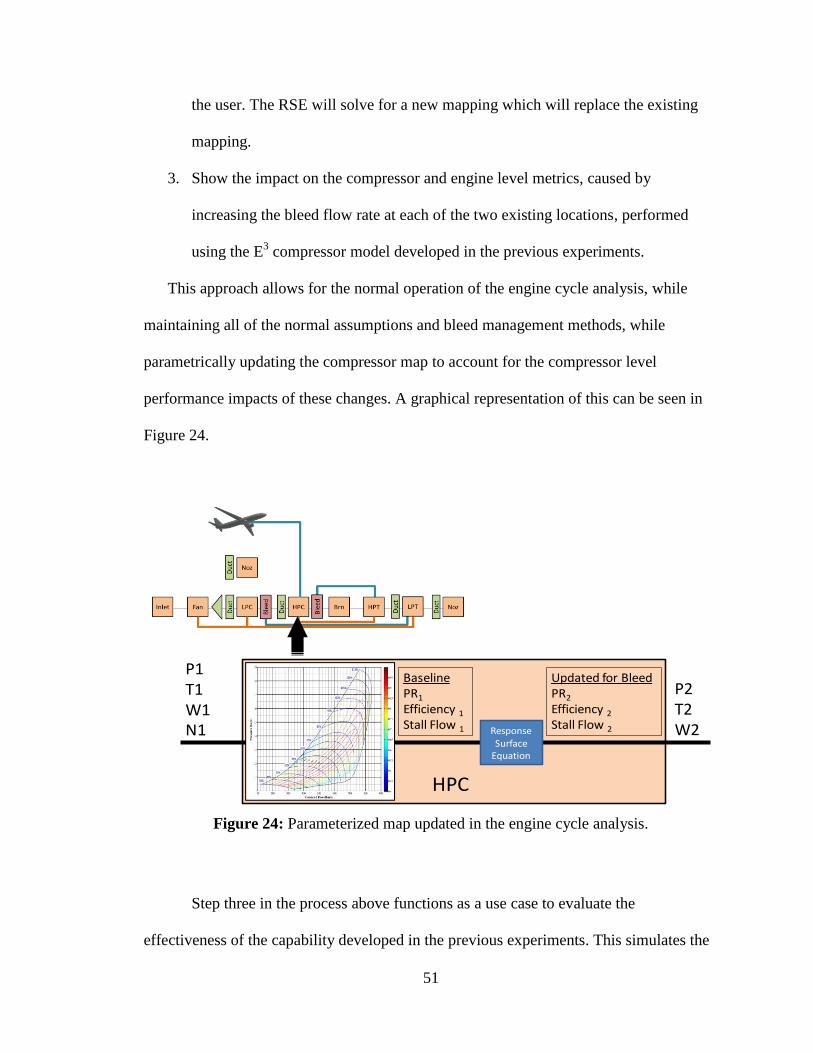
51

the user. The RSE will solve for a new mapping which will replace the existing

mapping.

3. Show the impact on the compressor and engine level metrics, caused by

increasing the bleed flow rate at each of the two existing locations, performed

using the E3 compressor model developed in the previous experiments.

This approach allows for the normal operation of the engine cycle analysis, while

maintaining all of the normal assumptions and bleed management methods, while

parametrically updating the compressor map to account for the compressor level

performance impacts of these changes. A graphical representation of this can be seen in

Figure 24.

Figure 24: Parameterized map updated in the engine cycle analysis.

Step three in the process above functions as a use case to evaluate the

effectiveness of the capability developed in the previous experiments. This simulates the

P1T1W1N1

P2T2W2Response

Surface Equation

BaselinePR1

Efficiency 1

Stall Flow 1

Updated for BleedPR2

Efficiency 2

Stall Flow 2

HPC

52

use of this capability in its intended environment, determining the full engine level

impacts in the presence of stricter bleed flow requirements. Additionally, utilization of

this developed capability in the engine design environment will reveal compressor level

impacts that are only visible in this environment. An example of this, includes the case

where the stall margin, a quality which is unique to an individual operating state, may be

found to be unsatisfactorily low at a point on the operating line, only visible through an

engine cycle analysis.

The engine model used for this experiment is of a similar performance class to the

GE90 [80]. This model will be performed under a condition representative of the

maximum takeoff rating, where the turbine entrance temperature and altitude will be held

constant at 3300 ⁰ F and 5000ft respectively. This model, the same as is depicted in

Figure 24, will be evaluated under 3 conditions, with regards to engine level performance

and operability, measured here by TSFC and stall margin, respectively. In addition, these

three conditions will be compared on the basis of their operating line, considered both a

performance and an operability metric, which effectively maps the operating state of the

compressor throughout the duration of any flight segment.

The first condition evaluated will stand as a baseline case. Here, the bleed flows

needed for turbine cooling are extracted from the compressor, without the extraction of

any additional customer bleed. Following this, the model will be operated under the same

bleed conditions but with the addition of 5% of the fifth stage discharge flow being

extracted for customer purposes. This will be conducted using the traditional cycle design

methodology, where the bleed extraction impacts the engine cycle, but the compressor

map remains identical to the map used in the first condition. Finally the validity of this

53

assumption will be assessed by performing the engine model under the same conditions

as in the previous condition, where cooling bleed and the additional 5% of the fifth stage

discharge bleed were extracted. The only difference is that the compressor performance

mapping will be replaced with the mapping which more appropriately fits this bleed

condition, using the RSEs developed in the previous experiment.

This final experiment is intended to reveal the capability of this design tool once

implemented in an engine level design environment. It is expected that large

discrepancies in performance and operability will appear when comparing the method of

updating maps, to the static mapping engine analysis method. This comparison between

the existing and the proposed methodologies will be the cornerstone of this research

endeavor. Upon successful completion, given reasonable results, this methodology will

be proven adequate in the case of providing a tool to answer the overarching question

fueling this research endeavor:

In the conceptual design phase, how does one determine the minimum core size to

meet engine performance and operability while accounting for subsystem bleed

requirements?

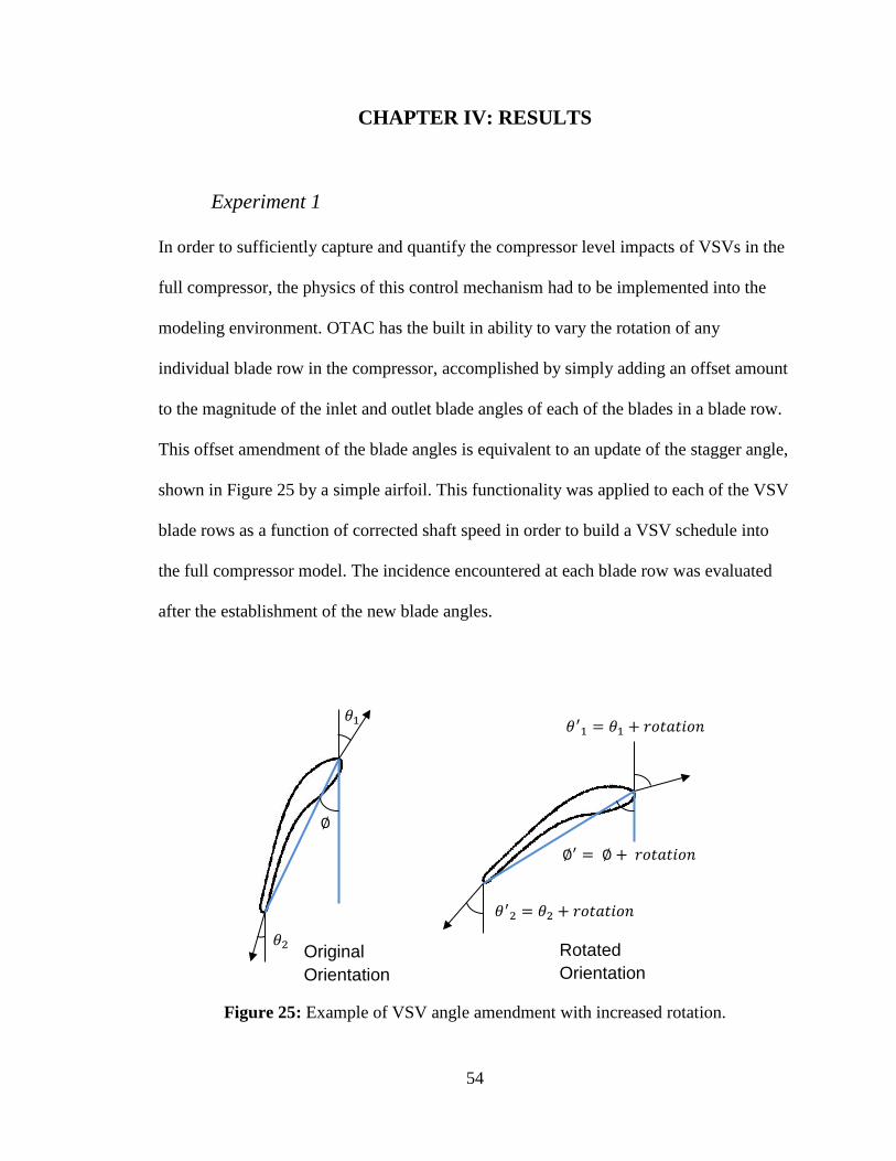
54

CHAPTER IV: RESULTS

Experiment 1

In order to sufficiently capture and quantify the compressor level impacts of VSVs in the

full compressor, the physics of this control mechanism had to be implemented into the

modeling environment. OTAC has the built in ability to vary the rotation of any

individual blade row in the compressor, accomplished by simply adding an offset amount

to the magnitude of the inlet and outlet blade angles of each of the blades in a blade row.

This offset amendment of the blade angles is equivalent to an update of the stagger angle,

shown in Figure 25 by a simple airfoil. This functionality was applied to each of the VSV

blade rows as a function of corrected shaft speed in order to build a VSV schedule into

the full compressor model. The incidence encountered at each blade row was evaluated

after the establishment of the new blade angles.

Figure 25: Example of VSV angle amendment with increased rotation.

𝜃2

∅′ = ∅ + 𝑟𝑜𝑡𝑎𝑡𝑖𝑜𝑛

𝜃′1 = 𝜃1 + 𝑟𝑜𝑡𝑎𝑡𝑖𝑜𝑛

𝜃′2 = 𝜃2 + 𝑟𝑜𝑡𝑎𝑡𝑖𝑜𝑛

𝜃1

∅

Rotated

Orientation

Original

Orientation

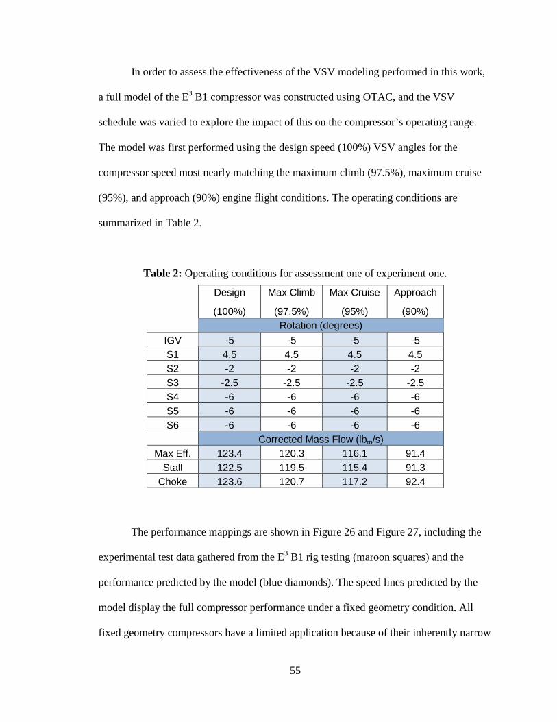
55

In order to assess the effectiveness of the VSV modeling performed in this work,

a full model of the E3 B1 compressor was constructed using OTAC, and the VSV

schedule was varied to explore the impact of this on the compressor’s operating range.

The model was first performed using the design speed (100%) VSV angles for the

compressor speed most nearly matching the maximum climb (97.5%), maximum cruise

(95%), and approach (90%) engine flight conditions. The operating conditions are

summarized in Table 2.

Table 2: Operating conditions for assessment one of experiment one.

Design

(100%)

Max Climb

(97.5%)

Max Cruise

(95%)

Approach

(90%)

Rotation (degrees)

IGV -5 -5 -5 -5

S1 4.5 4.5 4.5 4.5

S2 -2 -2 -2 -2

S3 -2.5 -2.5 -2.5 -2.5

S4 -6 -6 -6 -6

S5 -6 -6 -6 -6

S6 -6 -6 -6 -6


Max Eff. 123.4 120.3 116.1 91.4

Stall 122.5 119.5 115.4 91.3

Choke 123.6 120.7 117.2 92.4

The performance mappings are shown in Figure 26 and Figure 27, including the

experimental test data gathered from the E3 B1 rig testing (maroon squares) and the

performance predicted by the model (blue diamonds). The speed lines predicted by the

model display the full compressor performance under a fixed geometry condition. All

fixed geometry compressors have a limited application because of their inherently narrow

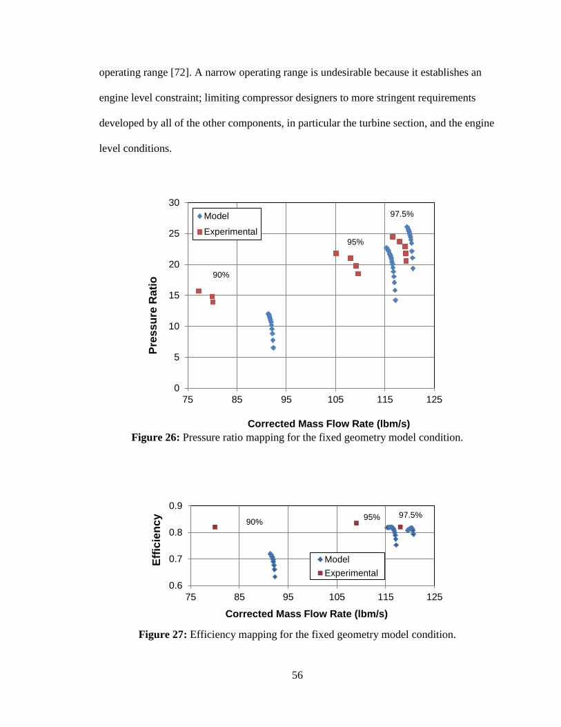
56

operating range [72]. A narrow operating range is undesirable because it establishes an

engine level constraint; limiting compressor designers to more stringent requirements

developed by all of the other components, in particular the turbine section, and the engine

level conditions.

Figure 26: Pressure ratio mapping for the fixed geometry model condition.

Figure 27: Efficiency mapping for the fixed geometry model condition.

0

5

10

15

20

25

30

75 85 95 105 115 125

Pre

ss

ure

Rati

o


Model

Experimental

0.6

0.7

0.8

0.9

75 85 95 105 115 125

Eff

icie

ncy


Model

Experimental

97.5%

95%

90%

97.5% 95% 90%

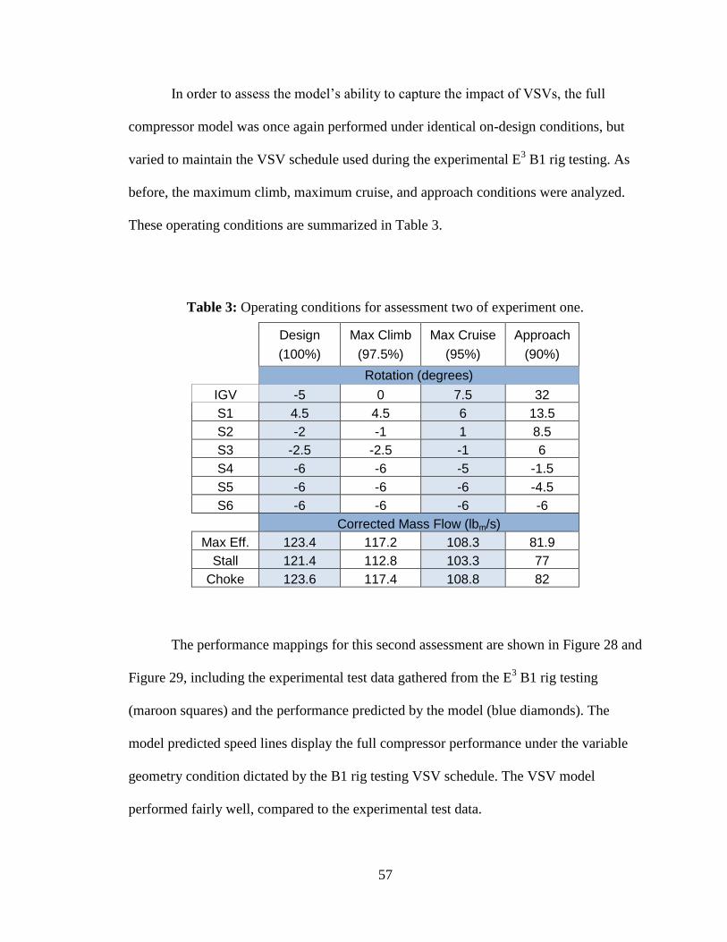
57

In order to assess the model’s ability to capture the impact of VSVs, the full

compressor model was once again performed under identical on-design conditions, but

varied to maintain the VSV schedule used during the experimental E3 B1 rig testing. As

before, the maximum climb, maximum cruise, and approach conditions were analyzed.

These operating conditions are summarized in Table 3.

Table 3: Operating conditions for assessment two of experiment one.

Design

(100%)

Max Climb

(97.5%)

Max Cruise

(95%)

Approach

(90%)

Rotation (degrees)

IGV -5 0 7.5 32

S1 4.5 4.5 6 13.5

S2 -2 -1 1 8.5

S3 -2.5 -2.5 -1 6

S4 -6 -6 -5 -1.5

S5 -6 -6 -6 -4.5

S6 -6 -6 -6 -6


Max Eff. 123.4 117.2 108.3 81.9

Stall 121.4 112.8 103.3 77

Choke 123.6 117.4 108.8 82

The performance mappings for this second assessment are shown in Figure 28 and

Figure 29, including the experimental test data gathered from the E3 B1 rig testing

(maroon squares) and the performance predicted by the model (blue diamonds). The

model predicted speed lines display the full compressor performance under the variable

geometry condition dictated by the B1 rig testing VSV schedule. The VSV model

performed fairly well, compared to the experimental test data.

58

Figure 28: Pressure ratio mapping for the variable geometry model condition.

Figure 29: Efficiency mapping for the variable geometry model condition.

Table 4 displays a comparison of the first (fixed geometry) and the second (VSV)

case to the experimental data, with respect to flow characteristics and operating range.

The implementation of the VSV modeling proved to predict the flow range variables

more effectively than the case without VSV modeling. Substantial improvement at

operating conditions further away from the design condition add confidence to the

0

5

10

15

20

25

30

75 85 95 105 115 125

Pre

ss

ure

Ra

tio


Model

Experimental

0.6

0.7

0.8

0.9

75 85 95 105 115 125

Eff

icie

ncy


Model

Experimental

95% 97.5%

90%

95% 97.5% 90%

59

models capability to properly capture the physics of the problem, reducing the error in

approach speed stall flow from 18.1% to 0.4% for example. Additionally, the second

case, utilizing VSVs, remained within an average point to point error of 1.5% with a

maximum error of 3.3%, lending confidence to the model for the purposes of this study.

It is important to note that there are many parameters impacting this model. The

magnitude of the performance shows clear discrepancies between the model and the test

data, which are likely the result of a variety of parameters, not essential to the goal of this

study, including loss, incidence (with respect to total magnitude), deviation, blockage,

and clearance modeling, amongst others. These parameters were defaulted within reason,

or utilized basic models, including a collection of loss models that may not be ideal for

such a highly loaded compressor.

Table 4: Comparison of variable to fixed geometry prediction performance.

Max Climb

(97.5%)

Max Cruise

(95%)

Approach

(90%)

Experimental B1 Test Rig Data (lbm/s)

Max Eff. 118 109 80

Stall 116.6 105.1 77.3

Choke 119.3 109.6 80.1

Case 1 : Fixed Geometry (% Error)

Max Eff. 1.9 6.5 14.3

Stall 2.5 9.8 18.1

Choke 1.2 6.9 15.4

Case 2 : VSV (% Error)

Max Eff. 0.7 0.6 2.4

Stall 3.3 1.7 0.4

Choke 1.6 0.7 2.4

60

The first two cases served to assess the model’s ability to predict the flow

performance of the full compressor using the geometry, flow conditions, and VSV

schedule of the experimental rig testing. A final study to assess the VSV modeling

proficiency was performed by varying the full VSV model by 10% of its total range in

each direction from the orientations used in case 2, for the same operating ranges. The

behavior of the speedlines should follow the trends found in the NACA 8 Stage study,

with respect to flow performance. The NACA 8 Stage study was performed in 1944 with

interest in the performance impacts of VSVs. Various VSV orientations were

experimentally tested under different loading conditions, on a compressor which is

significantly different from the E3, with respect to pressure and flow performance. [72]

Three tests conducted during the NACA 8 Stage project are of particular use in

determining whether or not the VSV model used in this work is properly predicting the

correct flow trends. The first test operated the full compressor test article at 75% of the

design speed, fixed geometry selected for the design condition, and an inlet Mach number

of 0.5. After empirically constructing the performance mapping for this condition, the

compressor was operated under the same condition as before, but with the VSVs re-

oriented to create an aerodynamic loading of 0.48. This required the VSVs to be closed as

much as 20 degrees in the front stages, and opened as much as 6 degrees in the rear

stages. After empirically constructing the performance mapping for this condition, the

compressor was once again varied, operating under the same conditions as before but

with the VSVs re-oriented to achieve an aerodynamic loading of 0.68. This required the

VSVs to be closed slightly in the front stages, up to 7 degrees, and to be opened in the

back stages to as much as 23 degrees. As a generalization, the speedlines are expected to

61

shift to lower operating flows, or left on the map, when closed, such as in the .48 loading

case. The opposite is also true that the speedlines are expected to shift to higher operating

flows when opened, such as in the .68 loading case. These trends are apparent in figure

30, showing the digitized performance mapping of the three cases discussed.

Figure 30: NACA 8 Stage performance mapping for VSV impact exploration.

In order to assess the capability of the VSV model to capture these trends, the

compressor model used in the previous cases was operated with the VSV settings

changed to first 10% opened, and then 10% closed from the design VSV settings. The

VSV settings range from -50% to 150% of the normal design VSV schedule. This means

that VSV orientations still vary with the corrected shaft speed, but that the variation is

proportionally ranged across all of the speeds, shown in Figure 80, in Appendix B. The

1

1.1

1.2

1.3

1.4

1.5

1.6

1.7

1.8

3000 3400 3800 4200 4600 5000

Pre

ss

ure

Rati

o

Volumetric Flow Rate (Ft3 /rev)

Design

Loading : .65

Loading : .48

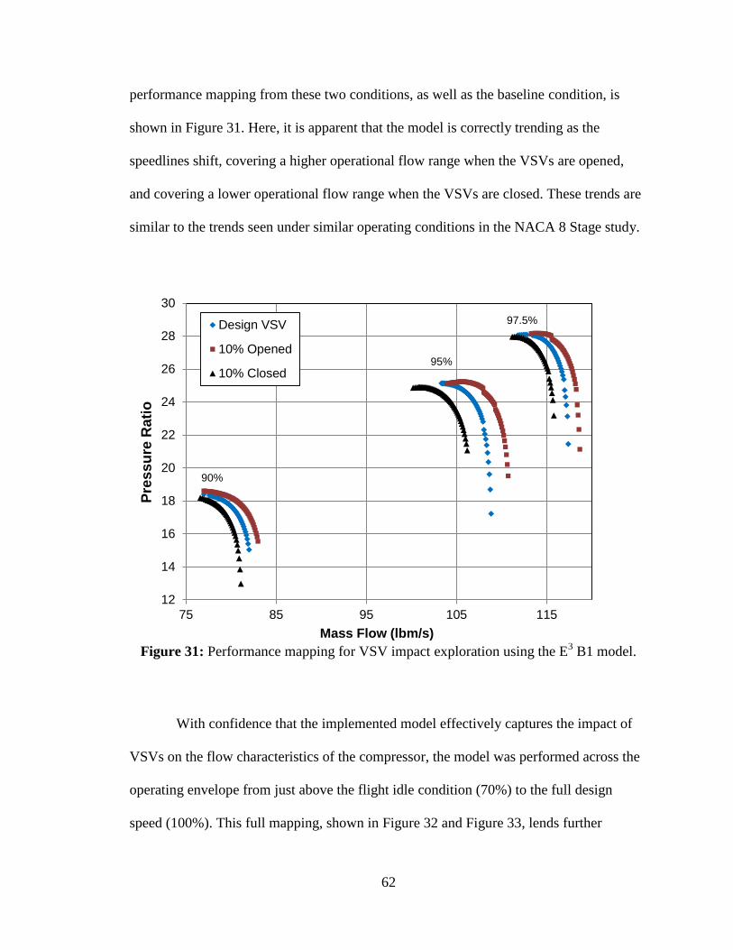
62

performance mapping from these two conditions, as well as the baseline condition, is

shown in Figure 31. Here, it is apparent that the model is correctly trending as the

speedlines shift, covering a higher operational flow range when the VSVs are opened,

and covering a lower operational flow range when the VSVs are closed. These trends are

similar to the trends seen under similar operating conditions in the NACA 8 Stage study.

Figure 31: Performance mapping for VSV impact exploration using the E

3 B1 model.

With confidence that the implemented model effectively captures the impact of

VSVs on the flow characteristics of the compressor, the model was performed across the

operating envelope from just above the flight idle condition (70%) to the full design

speed (100%). This full mapping, shown in Figure 32 and Figure 33, lends further

12

14

16

18

20

22

24

26

28

30

75 85 95 105 115

Pre

ss

ure

Ra

tio

Mass Flow (lbm/s)

Design VSV

10% Opened

10% Closed

97.5%

95%

90%

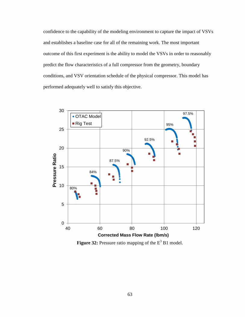
63

confidence to the capability of the modeling environment to capture the impact of VSVs

and establishes a baseline case for all of the remaining work. The most important

outcome of this first experiment is the ability to model the VSVs in order to reasonably

predict the flow characteristics of a full compressor from the geometry, boundary

conditions, and VSV orientation schedule of the physical compressor. This model has

performed adequately well to satisfy this objective.

Figure 32: Pressure ratio mapping of the E

3 B1 model.

0

5

10

15

20

25

30

40 60 80 100 120

Pre

ss

ure

Rati

o


OTAC Model

Rig Test 95%

97.5%

92.5%

90%

87.5%

84%

80%

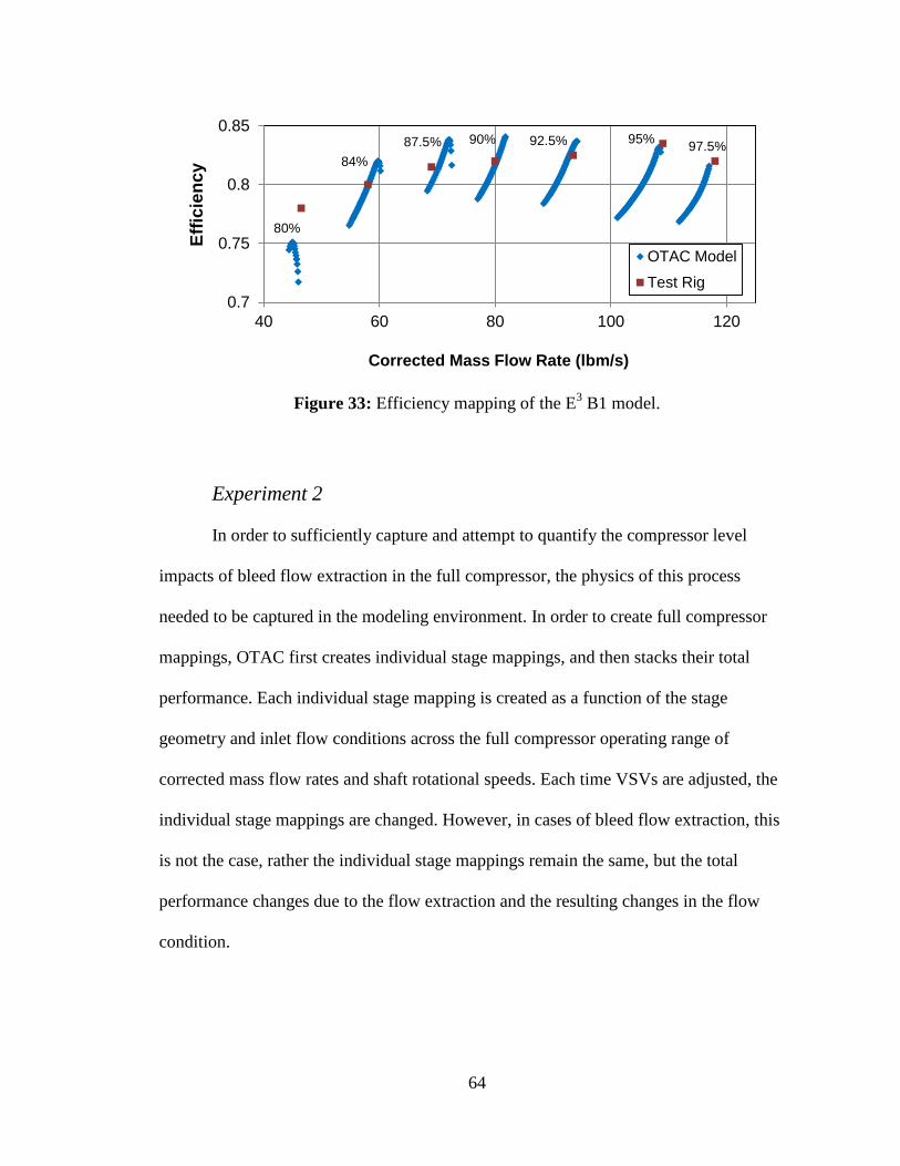
64

Figure 33: Efficiency mapping of the E

3 B1 model.

Experiment 2

In order to sufficiently capture and attempt to quantify the compressor level

impacts of bleed flow extraction in the full compressor, the physics of this process

needed to be captured in the modeling environment. In order to create full compressor

mappings, OTAC first creates individual stage mappings, and then stacks their total

performance. Each individual stage mapping is created as a function of the stage

geometry and inlet flow conditions across the full compressor operating range of

corrected mass flow rates and shaft rotational speeds. Each time VSVs are adjusted, the

individual stage mappings are changed. However, in cases of bleed flow extraction, this

is not the case, rather the individual stage mappings remain the same, but the total

performance changes due to the flow extraction and the resulting changes in the flow

condition.

0.7

0.75

0.8

0.85

40 60 80 100 120

Eff

icie

ncy


OTAC Model

Test Rig

97.5% 95% 92.5% 90% 87.5%

84%

80%

65

Model Construction

When bleed flow is extracted, there are a variety of thermodynamic and

aerodynamic impacts on the remaining flow in the compressor. These can be explained

comprehensively in the context of a walkthrough of the modeling approach used to

capture the bleed flow extraction process. As explained before, the compressor model

constructed in OTAC utilizes five individual streamlines to capture a higher fidelity

response than would be available in a single streamline analysis. This is managed by

establishing the compressor entrance boundary conditions which define a single, mid-

radius streamline, and breaking this streamline into the five new streamlines of interest,

shown in figure 34. These streamlines are sized to maintain equal mass flow rate, and to

maintain all of the thermodynamic total properties, as well as the meridional flow angle

of the original streamline. In order to preserve continuity between the individual streams,

the mean radius of each stream is varied. Finally, any swirl in the single stream results in

the variation of the tangential flow angle and Mach number of each of the individual

streams to establish a free vortex flow condition [76]. Upon completion of this expansion,

there remain five individual flow streams exhibiting qualities more closely paralleling the

actual flow qualities which would be expected in a physical compressor than those

captured by a single, mid radius streamline.

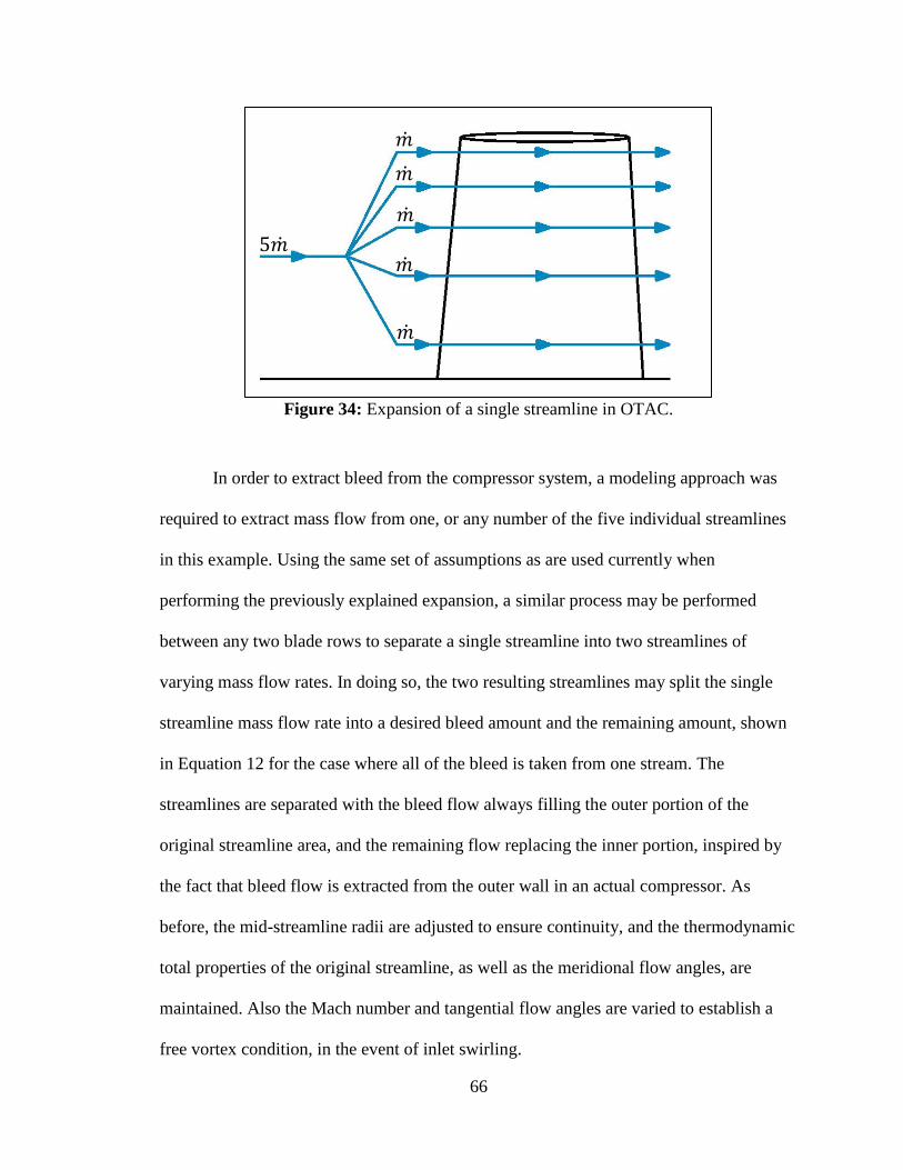
66

Figure 34: Expansion of a single streamline in OTAC.

In order to extract bleed from the compressor system, a modeling approach was

required to extract mass flow from one, or any number of the five individual streamlines

in this example. Using the same set of assumptions as are used currently when

performing the previously explained expansion, a similar process may be performed

between any two blade rows to separate a single streamline into two streamlines of

varying mass flow rates. In doing so, the two resulting streamlines may split the single

streamline mass flow rate into a desired bleed amount and the remaining amount, shown

in Equation 12 for the case where all of the bleed is taken from one stream. The

streamlines are separated with the bleed flow always filling the outer portion of the

original streamline area, and the remaining flow replacing the inner portion, inspired by

the fact that bleed flow is extracted from the outer wall in an actual compressor. As

before, the mid-streamline radii are adjusted to ensure continuity, and the thermodynamic

total properties of the original streamline, as well as the meridional flow angles, are

maintained. Also the Mach number and tangential flow angles are varied to establish a

free vortex condition, in the event of inlet swirling.

𝑚

𝑚

𝑚

𝑚

𝑚

5𝑚

67

𝑊𝐵𝑙𝑒𝑒𝑑 = 5 ∗ 𝑊 ∗ (%𝐵𝑙𝑒𝑒𝑑)

𝑊𝑅𝑒𝑚𝑎𝑖𝑛𝑖𝑛𝑔 = 𝑊 −𝑊𝐵𝑙𝑒𝑒𝑑 (12)

The separation of the original streamline results in the creation of two new

streamlines, sized to the desired bleed flow and to the remaining flow, respectively. The

streamline which is sized for the desired bleed flow may be terminated at this point, by

connection to a “FlowEnd” element, which establishes a sink for a single fluid

streamline. The remaining streamline must then be expanded to fill the space left by the

extracted bleed flow streamline, which may be accomplished by similar means to those

used to reduce the five streamlines at the back end of the compressor. This reduction

maintains the mass flow rate, stagnation enthalpy, tangential momentum, and through

flow impulse, and recalculates a new mid-streamline radius and area. In addition, the

streamline’s tangential flow angle, Mach number, and stagnation pressure are varied to

match the existing angular momentum, impulse, and area [77]. Upon completion of this

process, shown in Figure 35, the full compressor will maintain five streamlines, one of

the five containing less mass flow from bleed extraction, before entering the next blade

row in the system.

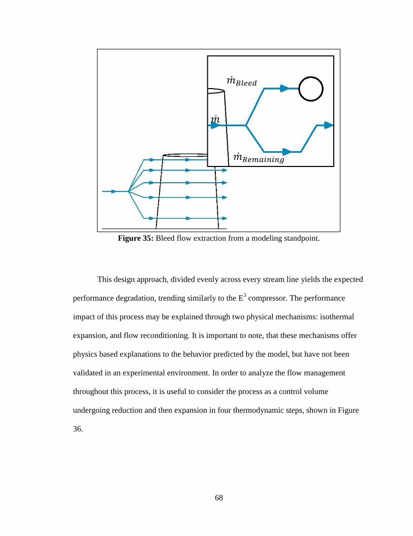
68

Figure 35: Bleed flow extraction from a modeling standpoint.

This design approach, divided evenly across every stream line yields the expected

performance degradation, trending similarly to the E3 compressor. The performance

impact of this process may be explained through two physical mechanisms: isothermal

expansion, and flow reconditioning. It is important to note, that these mechanisms offer

physics based explanations to the behavior predicted by the model, but have not been

validated in an experimental environment. In order to analyze the flow management

throughout this process, it is useful to consider the process as a control volume

undergoing reduction and then expansion in four thermodynamic steps, shown in Figure

36.

𝑚

𝑚 𝐵𝑙𝑒𝑒𝑑

𝑚 𝑅𝑒𝑚𝑎𝑖𝑛𝑖𝑛𝑔

69

Figure 36: Thermodynamic response to bleed flow extraction.

First, the control volume maintains all of the properties of the pre-separated

streamline, including the volumetric flow rate (𝑄 ), the static pressure (𝑃𝑠), and the static

temperature (𝑇𝑆). Next, the control volume is divided into two separate control volumes

containing the bleed flow and the remaining flow respectively. Following this, the bleed

air is removed from the system, vacating the control volume which contained the bleed

flow. Finally, the partition between the two control volumes is instantaneously removed,

leaving the remaining flow to completely fill the control volume. In doing so, the

temperature of the flow remains constant, which considering air to be a nearly ideal gas,

conforms to Boyle’s Law for isothermal expansion, shown in Equation 13. In addition,

the control volume expands, and the static pressure of the flow is reduced, shown in

Equation 14 and Equation 15. This final step accounts for the overall performance

degradation in the system.

𝑇𝑆𝐹𝑖𝑛𝑎𝑙 = 𝑇𝑆𝑅 (13)

𝑄 𝐼𝑛𝑖𝑡𝑖𝑎𝑙

𝑃𝑆𝐼𝑛𝑖𝑡𝑖𝑎𝑙

𝑇𝑆𝐼𝑛𝑖𝑡𝑖𝑎𝑙

𝑄 𝐵𝑙𝑒𝑒𝑑

𝑃𝑆𝐵𝑙𝑒𝑒𝑑

𝑇𝑆𝐵𝑙𝑒𝑒𝑑

𝑄 𝑅𝑒𝑚𝑎𝑖𝑛

𝑃𝑆𝑅𝑒𝑚𝑎𝑖𝑛

𝑇𝑆𝑅𝑒𝑚𝑎𝑖𝑛 𝑄 𝑅𝑒𝑚𝑎𝑖𝑛

𝑃𝑆𝑅𝑒𝑚𝑎𝑖𝑛

𝑇𝑆𝑅𝑒𝑚𝑎𝑖𝑛

𝑄 𝐵𝑙𝑒𝑒𝑑

𝑃𝑆𝐵𝑙𝑒𝑒𝑑

𝑇𝑆𝐵𝑙𝑒𝑒𝑑

𝑄 𝐹𝑖𝑛𝑎𝑙

𝑃𝑆𝐹𝑖𝑛𝑎𝑙

𝑇𝑆𝐹𝑖𝑛𝑎𝑙

Step 1 Step 2 Step 3 Step 4

70

𝑄 𝐹𝑖𝑛𝑎𝑙 = 𝑄 𝑅 + 𝑄 𝐵

(14)

𝑃𝑆𝐹𝑖𝑛𝑎𝑙 =

𝑃𝑆𝑅 ∗ 𝑚 𝑅

𝜌𝑆𝑅 (𝑚𝑅

𝜌𝑆𝑅+

𝑚𝐵

𝜌𝑆𝐵)

(15)

Three steps were developed as a method for capturing the impact of bleed flow

extraction on a compressor’s performance and operability:

1. Characterize each stage by an individual performance map.

2. Extract the desired bleed from the stations between any two stages.

3. Construct the full compressor performance mapping by combining each individual

stage performance map in a stage stacking process, accounting for the flow condition

into each individual stage.

OTAC is already designed to perform step 1 and step 3 above, so the construction

of the extraction model described above, in conjunction with the normal OTAC modeling

environment, sufficiently accomplishes these tasks. In order to assess the proper

operation of the bleed flow model, two small studies were performed using a simple two

stage compressor, incorporating bleed extraction after the first stage stator. For the sake

of these studies, the efficiency mapping has not been included since the pressure ratio and

efficiency will be coupled via the work input into the system as defined by Equation 16.

𝑃𝑅 = [𝜂𝐶 ∗ ∆𝐻

𝐶𝑝 𝑇𝑇1 ∗ 𝑔𝐽+ 1]

𝛾

𝛾−1

(16)

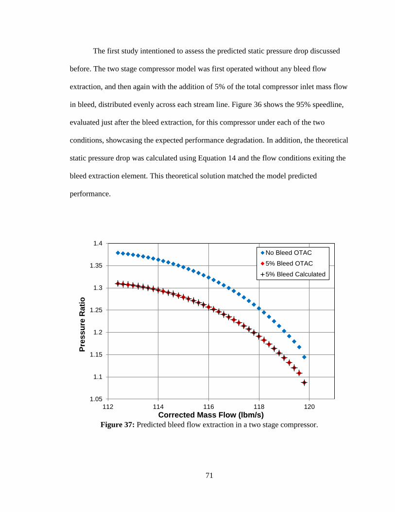
71

The first study intentioned to assess the predicted static pressure drop discussed

before. The two stage compressor model was first operated without any bleed flow

extraction, and then again with the addition of 5% of the total compressor inlet mass flow

in bleed, distributed evenly across each stream line. Figure 36 shows the 95% speedline,

evaluated just after the bleed extraction, for this compressor under each of the two

conditions, showcasing the expected performance degradation. In addition, the theoretical

static pressure drop was calculated using Equation 14 and the flow conditions exiting the

bleed extraction element. This theoretical solution matched the model predicted

performance.

Figure 37: Predicted bleed flow extraction in a two stage compressor.

1.05

1.1

1.15

1.2

1.25

1.3

1.35

1.4

112 114 116 118 120

Pre

ss

ure

Rati

o


No Bleed OTAC

5% Bleed OTAC

5% Bleed Calculated

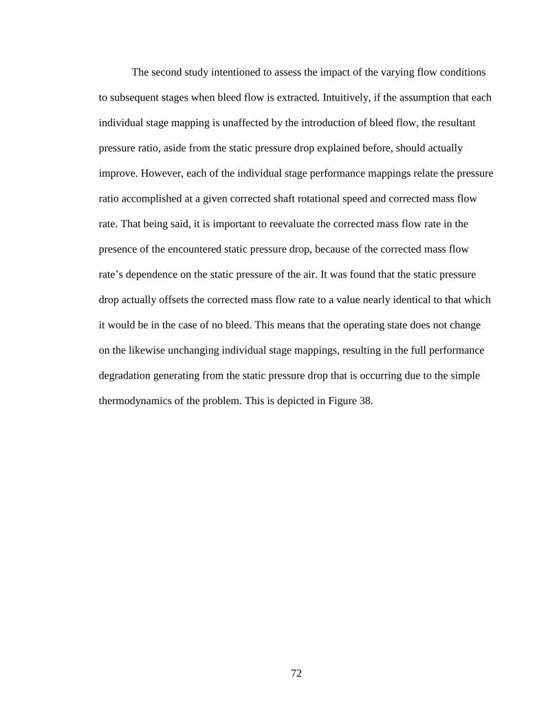
72

The second study intentioned to assess the impact of the varying flow conditions

to subsequent stages when bleed flow is extracted. Intuitively, if the assumption that each

individual stage mapping is unaffected by the introduction of bleed flow, the resultant

pressure ratio, aside from the static pressure drop explained before, should actually

improve. However, each of the individual stage performance mappings relate the pressure

ratio accomplished at a given corrected shaft rotational speed and corrected mass flow

rate. That being said, it is important to reevaluate the corrected mass flow rate in the

presence of the encountered static pressure drop, because of the corrected mass flow

rate’s dependence on the static pressure of the air. It was found that the static pressure

drop actually offsets the corrected mass flow rate to a value nearly identical to that which

it would be in the case of no bleed. This means that the operating state does not change

on the likewise unchanging individual stage mappings, resulting in the full performance

degradation generating from the static pressure drop that is occurring due to the simple

thermodynamics of the problem. This is depicted in Figure 38.

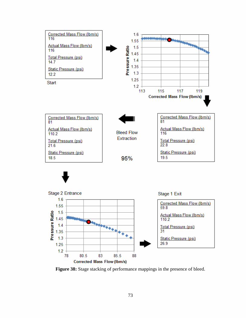
73

Figure 38: Stage stacking of performance mappings in the presence of bleed.

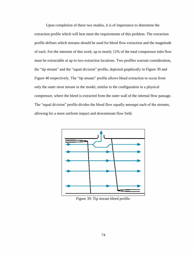
74

Upon completion of these two studies, it is of importance to determine the

extraction profile which will best meet the requirements of this problem. The extraction

profile defines which streams should be used for bleed flow extraction and the magnitude

of each. For the interests of this work, up to nearly 12% of the total compressor inlet flow

must be extractable at up to two extraction locations. Two profiles warrant consideration,

the “tip stream” and the “equal division” profile, depicted graphically in Figure 39 and

Figure 40 respectively. The “tip stream” profile allows bleed extraction to occur from

only the outer most stream in the model, similar to the configuration in a physical

compressor, where the bleed is extracted from the outer wall of the internal flow passage.

The “equal division” profile divides the bleed flow equally amongst each of the streams,

allowing for a more uniform impact and downstream flow field.

Figure 39: Tip stream bleed profile.

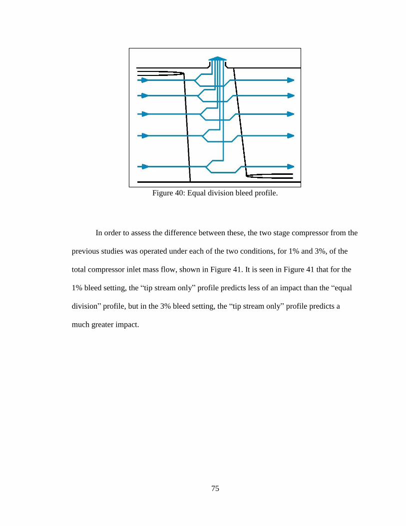
75

Figure 40: Equal division bleed profile.

In order to assess the difference between these, the two stage compressor from the

previous studies was operated under each of the two conditions, for 1% and 3%, of the

total compressor inlet mass flow, shown in Figure 41. It is seen in Figure 41 that for the

1% bleed setting, the “tip stream only” profile predicts less of an impact than the “equal

division” profile, but in the 3% bleed setting, the “tip stream only” profile predicts a

much greater impact.

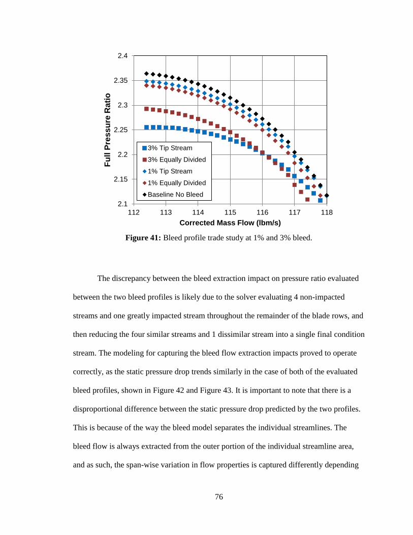
76

Figure 41: Bleed profile trade study at 1% and 3% bleed.

The discrepancy between the bleed extraction impact on pressure ratio evaluated

between the two bleed profiles is likely due to the solver evaluating 4 non-impacted

streams and one greatly impacted stream throughout the remainder of the blade rows, and

then reducing the four similar streams and 1 dissimilar stream into a single final condition

stream. The modeling for capturing the bleed flow extraction impacts proved to operate

correctly, as the static pressure drop trends similarly in the case of both of the evaluated

bleed profiles, shown in Figure 42 and Figure 43. It is important to note that there is a

disproportional difference between the static pressure drop predicted by the two profiles.

This is because of the way the bleed model separates the individual streamlines. The

bleed flow is always extracted from the outer portion of the individual streamline area,

and as such, the span-wise variation in flow properties is captured differently depending

2.1

2.15

2.2

2.25

2.3

2.35

2.4

112 113 114 115 116 117 118

Fu

ll P

res

su

re R

ati

o


3% Tip Stream

3% Equally Divided

1% Tip Stream

1% Equally Divided

Baseline No Bleed

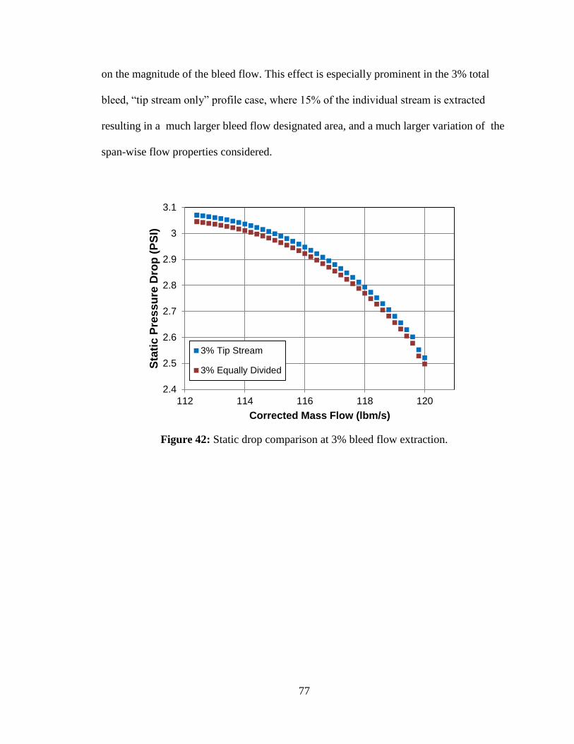
77

on the magnitude of the bleed flow. This effect is especially prominent in the 3% total

bleed, “tip stream only” profile case, where 15% of the individual stream is extracted

resulting in a much larger bleed flow designated area, and a much larger variation of the

span-wise flow properties considered.

Figure 42: Static drop comparison at 3% bleed flow extraction.

2.4

2.5

2.6

2.7

2.8

2.9

3

3.1

112 114 116 118 120

Sta

tic

Pre

ss

ure

Dro

p (

PS

I)


3% Tip Stream

3% Equally Divided

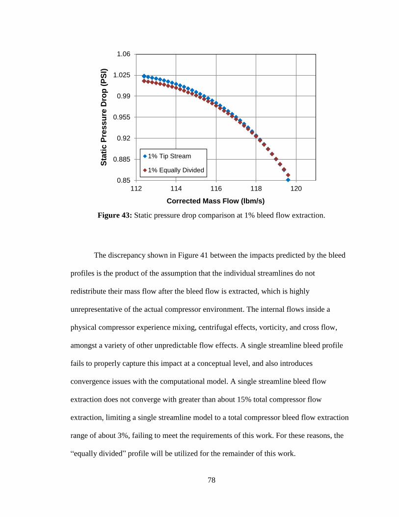
78

Figure 43: Static pressure drop comparison at 1% bleed flow extraction.

The discrepancy shown in Figure 41 between the impacts predicted by the bleed

profiles is the product of the assumption that the individual streamlines do not

redistribute their mass flow after the bleed flow is extracted, which is highly

unrepresentative of the actual compressor environment. The internal flows inside a

physical compressor experience mixing, centrifugal effects, vorticity, and cross flow,

amongst a variety of other unpredictable flow effects. A single streamline bleed profile

fails to properly capture this impact at a conceptual level, and also introduces

convergence issues with the computational model. A single streamline bleed flow

extraction does not converge with greater than about 15% total compressor flow

extraction, limiting a single streamline model to a total compressor bleed flow extraction

range of about 3%, failing to meet the requirements of this work. For these reasons, the

“equally divided” profile will be utilized for the remainder of this work.

0.85

0.885

0.92

0.955

0.99

1.025

1.06

112 114 116 118 120

Sta

tic

Pre

ss

ure

Dro

p (

PS

I)


1% Tip Stream

1% Equally Divided

79

Model Implementation and Assessment

The E3 B2 compressor incorporated design decisions made after the completion of

the B1 testing, developed to improve the existing performance and operating flow range.

The B2 testing consisted of the new compressor with changed bladeing, utilized a new

VSV schedule, and it is assumed to have operated with the addition of bleed. This design

condition incorporates the minimum bleed setting, wherein the necessary amount of

turbine blade cooling flow, 1.3% and 2.3% of the previous stage’s discharge flow was

extracted from two locations, placed just after the 5th

and 7th

stages respectively. The

changes made between the B1 and the B2 testing were concerned primarily with

extending the high speed stall margin. The performance remained relatively unchanged,

and as such, the assumption that the bleed addition is the main performance impact driver

will be carried for the purpose of assessing the model’s effectiveness, by comparing the

model to the experimental (empirical) test rig performance. The experimental test data

from both the B1 and B2 testing is shown in Figure 44, where the B2 test data has been

shifted to account for the VSVs being closed further during the B2 testing than in the B1

testing.

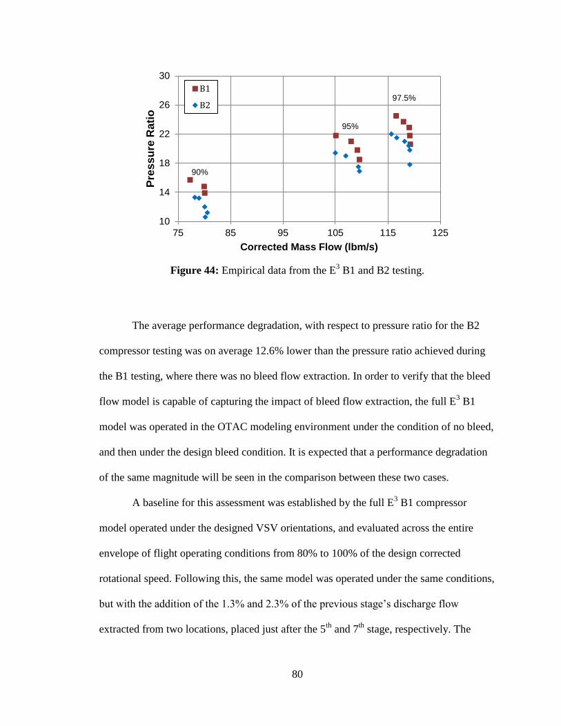
80

Figure 44: Empirical data from the E

3 B1 and B2 testing.

The average performance degradation, with respect to pressure ratio for the B2

compressor testing was on average 12.6% lower than the pressure ratio achieved during

the B1 testing, where there was no bleed flow extraction. In order to verify that the bleed

flow model is capable of capturing the impact of bleed flow extraction, the full E3 B1

model was operated in the OTAC modeling environment under the condition of no bleed,

and then under the design bleed condition. It is expected that a performance degradation

of the same magnitude will be seen in the comparison between these two cases.

A baseline for this assessment was established by the full E3 B1 compressor

model operated under the designed VSV orientations, and evaluated across the entire

envelope of flight operating conditions from 80% to 100% of the design corrected

rotational speed. Following this, the same model was operated under the same conditions,

but with the addition of the 1.3% and 2.3% of the previous stage’s discharge flow

extracted from two locations, placed just after the 5th

and 7th

stage, respectively. The

10

14

18

22

26

30

75 85 95 105 115 125

Pre

ss

ure

Rati

o


B1

B297.5%

95%

90%

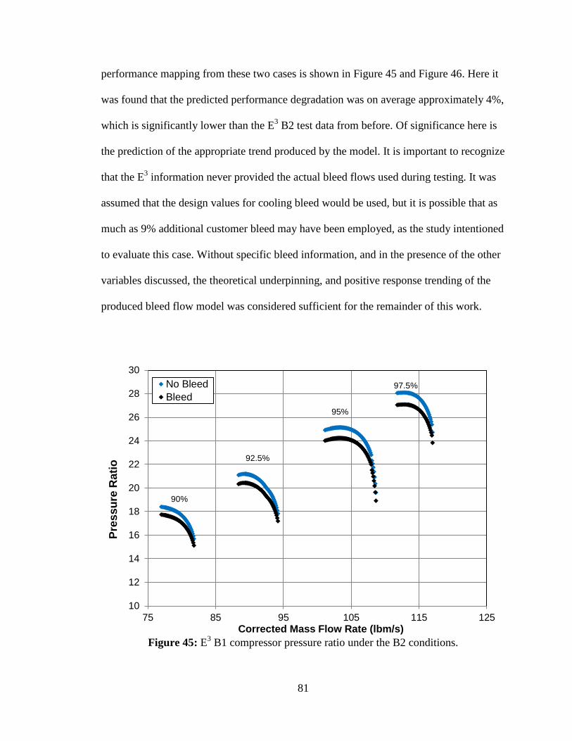
81

performance mapping from these two cases is shown in Figure 45 and Figure 46. Here it

was found that the predicted performance degradation was on average approximately 4%,

which is significantly lower than the E3 B2 test data from before. Of significance here is

the prediction of the appropriate trend produced by the model. It is important to recognize

that the E3 information never provided the actual bleed flows used during testing. It was

assumed that the design values for cooling bleed would be used, but it is possible that as

much as 9% additional customer bleed may have been employed, as the study intentioned

to evaluate this case. Without specific bleed information, and in the presence of the other

variables discussed, the theoretical underpinning, and positive response trending of the

produced bleed flow model was considered sufficient for the remainder of this work.

Figure 45: E

3 B1 compressor pressure ratio under the B2 conditions.

10

12

14

16

18

20

22

24

26

28

30

75 85 95 105 115 125

Pre

ss

ure

Rati

o


No Bleed

Bleed

90%

92.5%

95%

97.5%

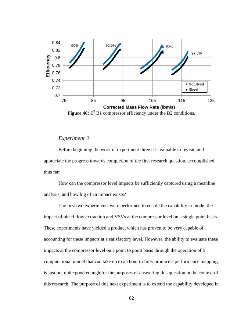
82

Figure 46: E

3 B1 compressor efficiency under the B2 conditions.

Experiment 3

Before beginning the work of experiment three it is valuable to revisit, and

appreciate the progress towards completion of the first research question, accomplished

thus far:

How can the compressor level impacts be sufficiently captured using a meanline


The first two experiments were performed to enable the capability to model the

impact of bleed flow extraction and VSVs at the compressor level on a single point basis.

These experiments have yielded a product which has proven to be very capable of

accounting for these impacts at a satisfactory level. However, the ability to evaluate these

impacts at the compressor level on a point to point basis through the operation of a

computational model that can take up to an hour to fully produce a performance mapping,

is just not quite good enough for the purposes of answering this question in the context of

this research. The purpose of this next experiment is to extend the capability developed in

0.7

0.72

0.74

0.76

0.78

0.8

0.82

0.84

75 85 95 105 115 125

Eff

icie

ncy


No Bleed

Bleed

90% 92.5% 95%

97.5%

83

the first two experiments to allow a compressor designer to quickly quantify any number

of compressor level changes in bleed flow and VSV setting, enabling them to rapidly

evaluate trends among the parameter variations. This experiment is designed to be

performed in three parts:

1. Construct an LHD DoE and complete the compressor model analysis at

each condition specified therein.

2. Use this data to form a response surface equation relating each of the

variables to each of the compressor level metrics as seen in Equation 11.

3. Use this response surface to form a full mapping of the compressor at the

experiment 2 condition and compare this map to the known map. Then

show the impact on the performance map of increasing the bleed flow rate

at each location, and varying the VSV settings to their most extreme

conditions to assess the RSE’s ability to properly predict the expected

trends.

Design of Experiments

The first of the prescribed tasks calls for the construction of an LHC DoE. This

was performed using a statistical software package named JMP, which allows for the

systematic variation of a large number of variables into a wide variety of DoE designs

[81]. The DoE contains fifty cases, where the VSV setting, the 5th stage bleed flow rate

(B5), and the 7th stage bleed flow rate (B7) are each varied. Additionally, based on the

fact that the E3 compressor operates with customer bleed from only one location, either

the B5 or B7, only one of the two bleed flow locations was allowed to exceed their

respective cooling requirement per case. Since the actual E3 compressor extracts

84

customer bleed from only the B5 location, 80 percent of the DoE varied the B5 bleed

while the B7 bleed remained constant, while only 20% of the DoE varied the B7 bleed

while the B5 bleed remained constant. This was performed to increase the fidelity of the

RSEs with respect to the B5 bleed, at the expense of the B7 bleed fidelity, intended to

better capture the realistic conditions of the physical compressor. A small portion of this

DoE is shown in Table 5, while the full DoE may be found in Table B1 in Appendix B. A

graphical representation of this DoE is shown in Figure 47, where it is seen that the B5

bleed is varied uniformly with the VSV setting, as is true of the B7 bleed variation. The

B5 bleed vs VSV plane displays the greatest design space, created in this manner to

provide the highest fidelity to the variation of the B5 bleed flow. It is important to note

that the VSV parameter is in terms of the percent schedule change across the

aforementioned range of -50% to 150%. Each VSV changes according to the schedule of

all of the VSVs for each shaft speed, shown in Figure 80. Additionally, it is important to

note that the B5 and B7 bleed parameters are in terms of the percentage of the previous

stage discharge flow being extracted.

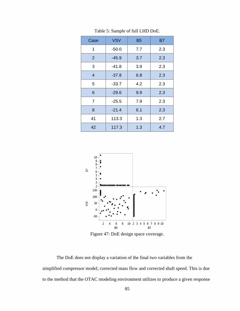
85

Table 5: Sample of full LHD DoE.

Case VSV B5 B7

1 -50.0 7.7 2.3

2 -45.9 3.7 2.3

3 -41.8 3.9 2.3

4 -37.8 6.8 2.3

5 -33.7 4.2 2.3

6 -29.6 9.9 2.3

7 -25.5 7.9 2.3

8 -21.4 6.1 2.3

41 113.3 1.3 2.7

42 117.3 1.3 4.7

Figure 47: DoE design space coverage.

The DoE does not display a variation of the final two variables from the

simplified compressor model; corrected mass flow and corrected shaft speed. This is due

to the method that the OTAC modeling environment utilizes to produce a given response

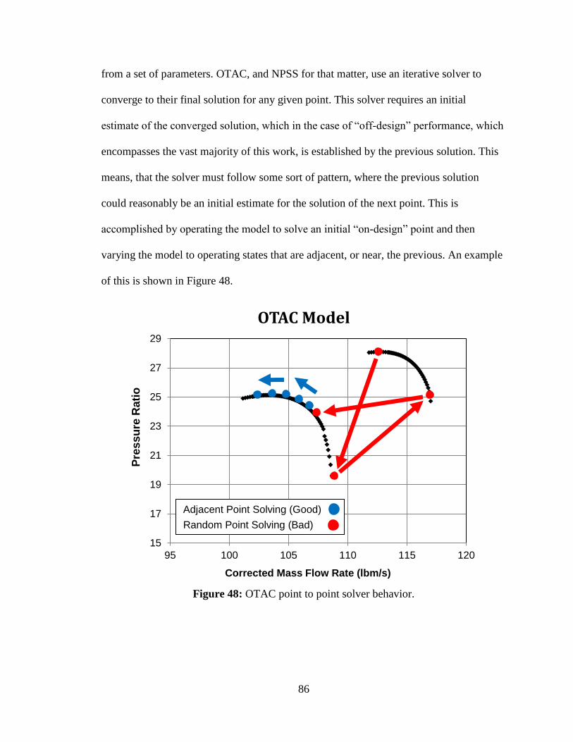
86

from a set of parameters. OTAC, and NPSS for that matter, use an iterative solver to

converge to their final solution for any given point. This solver requires an initial

estimate of the converged solution, which in the case of “off-design” performance, which

encompasses the vast majority of this work, is established by the previous solution. This

means, that the solver must follow some sort of pattern, where the previous solution

could reasonably be an initial estimate for the solution of the next point. This is

accomplished by operating the model to solve an initial “on-design” point and then

varying the model to operating states that are adjacent, or near, the previous. An example

of this is shown in Figure 48.

Figure 48: OTAC point to point solver behavior.

15

17

19

21

23

25

27

29

95 100 105 110 115 120

Pre

ss

ure

Rati

o


OTAC Model

Adjacent Point Solving (Good)

Random Point Solving (Bad)

87

The behavior of the solver imposes a constraint on the design space exploration,

where any corrected mass flow and corrected shaft speed variation must be linked and

performed in a predictable way. The constraint was managed by operating the model to

construct an entire performance mapping, through adjacent point to point solving, for

each of the individual cases defined by the DoE. This method produces 50 unique, full

compressor performance mappings, and approximately 11,000 unique point solutions.

Response Surface Equations

The second part of experiment three involves the simplification of the massive

collection of data found through the evaluation of the DoE. As discussed before, the

parameter variations and their associated responses may be represented by RSEs, also

called surrogate models here, producing simple mathematical formulas to represent the

behavior of the cumbersome and time consuming modeling environment. In order to

recreate a compressor mapping, a minimum of three surrogate models needed to be

developed, the first to predict the operating flows, and the rest to create the associated

pressure ratio and efficiencies.

To create the surrogate models a method called neural network modeling was

employed. This approach is identical for the purposes of this work to using response

surface methodology, and offers a very good method for forming the necessary surrogate

models. Neural networks are structured to find solutions by emulating the way that a

human brain solves problems, and are used to model multi-dimensional, highly nonlinear

systems [82]. Neural networks will be used in this experiment as the data is highly

nonlinear and contains many interactions that the surrogate models will need to

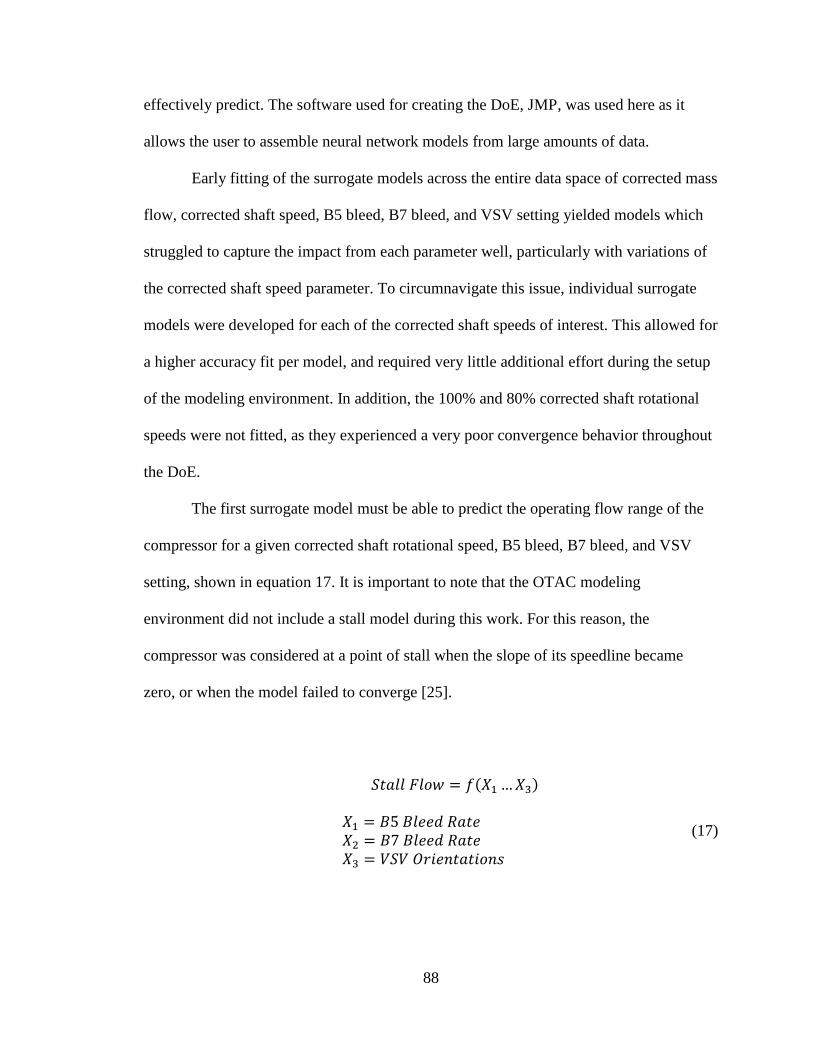
88

effectively predict. The software used for creating the DoE, JMP, was used here as it

allows the user to assemble neural network models from large amounts of data.

Early fitting of the surrogate models across the entire data space of corrected mass

flow, corrected shaft speed, B5 bleed, B7 bleed, and VSV setting yielded models which

struggled to capture the impact from each parameter well, particularly with variations of

the corrected shaft speed parameter. To circumnavigate this issue, individual surrogate

models were developed for each of the corrected shaft speeds of interest. This allowed for

a higher accuracy fit per model, and required very little additional effort during the setup

of the modeling environment. In addition, the 100% and 80% corrected shaft rotational

speeds were not fitted, as they experienced a very poor convergence behavior throughout

the DoE.

The first surrogate model must be able to predict the operating flow range of the

compressor for a given corrected shaft rotational speed, B5 bleed, B7 bleed, and VSV

setting, shown in equation 17. It is important to note that the OTAC modeling

environment did not include a stall model during this work. For this reason, the

compressor was considered at a point of stall when the slope of its speedline became

zero, or when the model failed to converge [25].

𝑆𝑡𝑎𝑙𝑙 𝐹𝑙𝑜𝑤 = 𝑓(𝑋1…𝑋3)

𝑋1 = 𝐵5 𝐵𝑙𝑒𝑒𝑑 𝑅𝑎𝑡𝑒



(17)

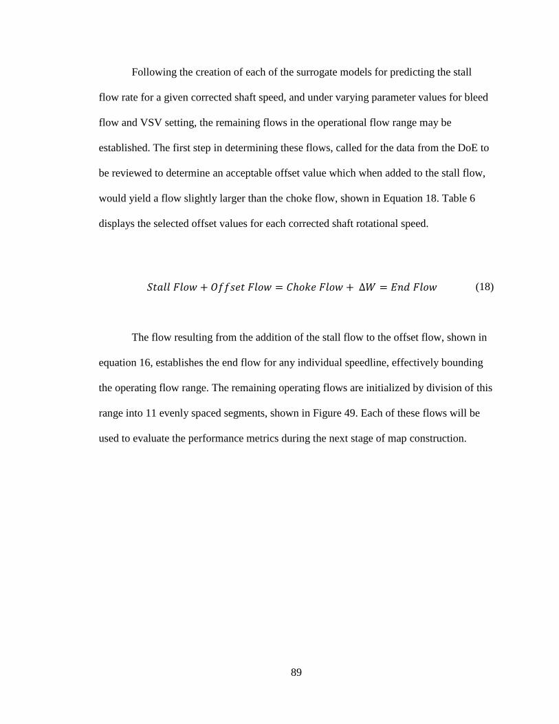
89

Following the creation of each of the surrogate models for predicting the stall

flow rate for a given corrected shaft speed, and under varying parameter values for bleed

flow and VSV setting, the remaining flows in the operational flow range may be

established. The first step in determining these flows, called for the data from the DoE to

be reviewed to determine an acceptable offset value which when added to the stall flow,

would yield a flow slightly larger than the choke flow, shown in Equation 18. Table 6

displays the selected offset values for each corrected shaft rotational speed.

𝑆𝑡𝑎𝑙𝑙 𝐹𝑙𝑜𝑤 + 𝑂𝑓𝑓𝑠𝑒𝑡 𝐹𝑙𝑜𝑤 = 𝐶ℎ𝑜𝑘𝑒 𝐹𝑙𝑜𝑤 + ∆𝑊 = 𝐸𝑛𝑑 𝐹𝑙𝑜𝑤 (18)

The flow resulting from the addition of the stall flow to the offset flow, shown in

equation 16, establishes the end flow for any individual speedline, effectively bounding

the operating flow range. The remaining operating flows are initialized by division of this

range into 11 evenly spaced segments, shown in Figure 49. Each of these flows will be

used to evaluate the performance metrics during the next stage of map construction.

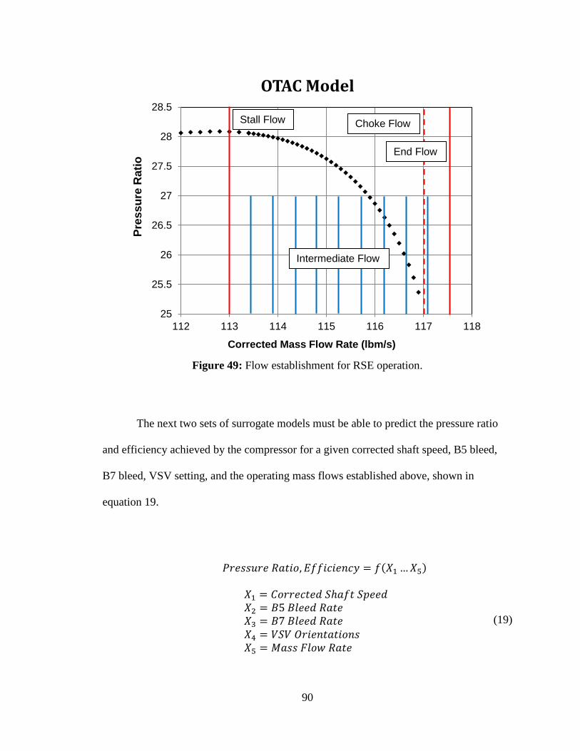
90

Figure 49: Flow establishment for RSE operation.

The next two sets of surrogate models must be able to predict the pressure ratio

and efficiency achieved by the compressor for a given corrected shaft speed, B5 bleed,

B7 bleed, VSV setting, and the operating mass flows established above, shown in

equation 19.

𝑃𝑟𝑒𝑠𝑠𝑢𝑟𝑒 𝑅𝑎𝑡𝑖𝑜, 𝐸𝑓𝑓𝑖𝑐𝑖𝑒𝑛𝑐𝑦 = 𝑓(𝑋1…𝑋5)

𝑋1 = 𝐶𝑜𝑟𝑟𝑒𝑐𝑡𝑒𝑑 𝑆ℎ𝑎𝑓𝑡 𝑆𝑝𝑒𝑒𝑑




𝑋5 = 𝑀𝑎𝑠𝑠 𝐹𝑙𝑜𝑤 𝑅𝑎𝑡𝑒

(19)

25

25.5

26

26.5

27

27.5

28

28.5

112 113 114 115 116 117 118

Pre

ss

ure

Rati

o


OTAC Model

Stall Flow Choke Flow

End Flow

Intermediate Flow

91

Upon completion of the surrogate modeling described to this point, a total of fifteen

surrogate models have been created, five each predicting the stall flow, pressure ratio,

and efficiency, of the compressor for corrected shaft speeds of 84%, 90%, 92.5%, 95%,

and 97.5% of the design corrected shaft speed. It is now necessary to investigate the

adequacy of each of the newly created surrogate models, in order to add credibility to the

performance, and to identify potential issues, of the model [45]. There are five key

metrics which define the adequacy of a surrogate model:

R2

Actual by Predicted Plot

Residual by Predicted Plot

Model Fit Error

Model Representation Error

These metrics may be best explained alongside the presentation of a surrogate

model which represents the average surrogate model constructed in this work. To this

end, the surrogate model created to predict the pressure ratio of the compressor at a

corrected shaft speed of 97.5% of the design shaft speed will be analyzed. The R2 value

represents the measure of the amount of variability accounted for by the model [45]. In

the case where a model perfectly captures all of the variability in a system, the associated

R2 value would be 1.0, however, the acceptable minimum for this value is 0.8 [45]. This

surrogate performed very well, achieving an R2 value of 0.9994, indicating a very good

fit thus far.

Following this, the actual by predicted and residual by predicted plots must be

evaluated, shown in Figure 50 and Figure 51. The actual by predicted plot displays the

92

known responses, found through the execution of the DoE, as compared to the responses

predicted by the surrogate model. An ideal fit is represented by the diagonal line, and it is

necessary for the test data to line up tightly along this line, as is seen in Figure 50. The

residual by predicted plot displays the error between the DoE responses used to generate

the surrogate model, and the responses predicted by the surrogate model. An adequate fit

should show a spattering of data, with no distinguishable patterns, and centered on zero.

The surrogate model performs well to accomplish this in Figure 51. It must be noted that

there are certain patterns observable in both of these plots which is an unavoidable

consequence of the adjacent point mapping constraint imposed by the modeling

environment used to produce the DoE data. Nonetheless, the surrogate model performs

well enough for the purposes of this work, with respect to these surrogate adequacy

metrics.

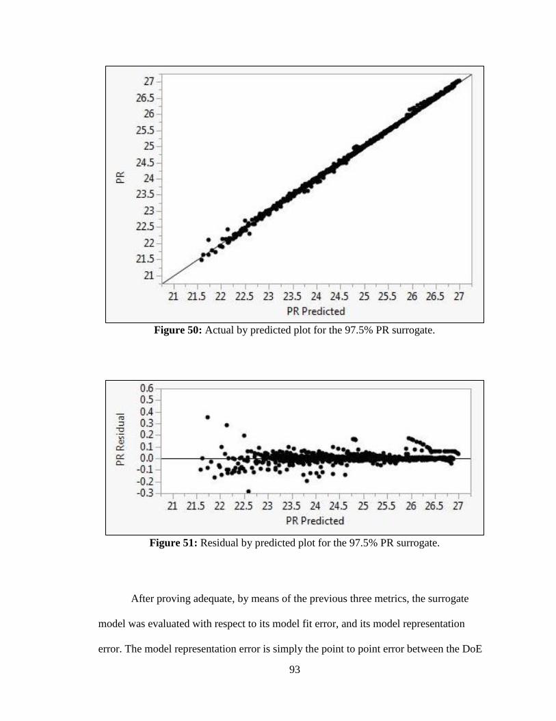
93

Figure 50: Actual by predicted plot for the 97.5% PR surrogate.

Figure 51: Residual by predicted plot for the 97.5% PR surrogate.

After proving adequate, by means of the previous three metrics, the surrogate

model was evaluated with respect to its model fit error, and its model representation

error. The model representation error is simply the point to point error between the DoE

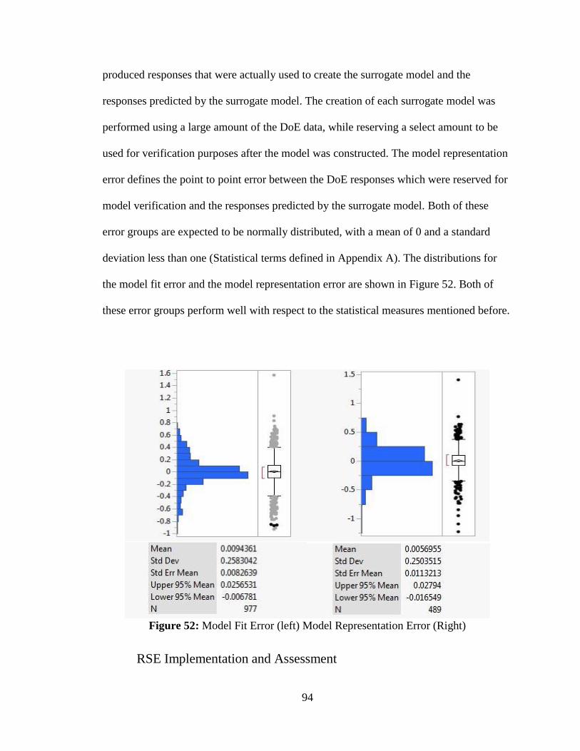
94

produced responses that were actually used to create the surrogate model and the

responses predicted by the surrogate model. The creation of each surrogate model was

performed using a large amount of the DoE data, while reserving a select amount to be

used for verification purposes after the model was constructed. The model representation

error defines the point to point error between the DoE responses which were reserved for

model verification and the responses predicted by the surrogate model. Both of these

error groups are expected to be normally distributed, with a mean of 0 and a standard

deviation less than one (Statistical terms defined in Appendix A). The distributions for

the model fit error and the model representation error are shown in Figure 52. Both of

these error groups perform well with respect to the statistical measures mentioned before.

Figure 52: Model Fit Error (left) Model Representation Error (Right)

RSE Implementation and Assessment

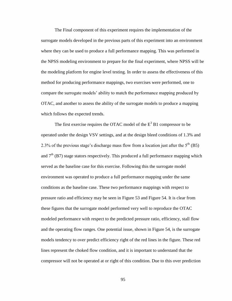
95

The Final component of this experiment requires the implementation of the

surrogate models developed in the previous parts of this experiment into an environment

where they can be used to produce a full performance mapping. This was performed in

the NPSS modeling environment to prepare for the final experiment, where NPSS will be

the modeling platform for engine level testing. In order to assess the effectiveness of this

method for producing performance mappings, two exercises were performed, one to

compare the surrogate models’ ability to match the performance mapping produced by

OTAC, and another to assess the ability of the surrogate models to produce a mapping

which follows the expected trends.

The first exercise requires the OTAC model of the E3 B1 compressor to be

operated under the design VSV settings, and at the design bleed conditions of 1.3% and

2.3% of the previous stage’s discharge mass flow from a location just after the 5th

(B5)

and 7th

(B7) stage stators respectively. This produced a full performance mapping which

served as the baseline case for this exercise. Following this the surrogate model

environment was operated to produce a full performance mapping under the same

conditions as the baseline case. These two performance mappings with respect to

pressure ratio and efficiency may be seen in Figure 53 and Figure 54. It is clear from

these figures that the surrogate model performed very well to reproduce the OTAC

modeled performance with respect to the predicted pressure ratio, efficiency, stall flow

and the operating flow ranges. One potential issue, shown in Figure 54, is the surrogate

models tendency to over predict efficiency right of the red lines in the figure. These red

lines represent the choked flow condition, and it is important to understand that the

compressor will not be operated at or right of this condition. Due to this over prediction

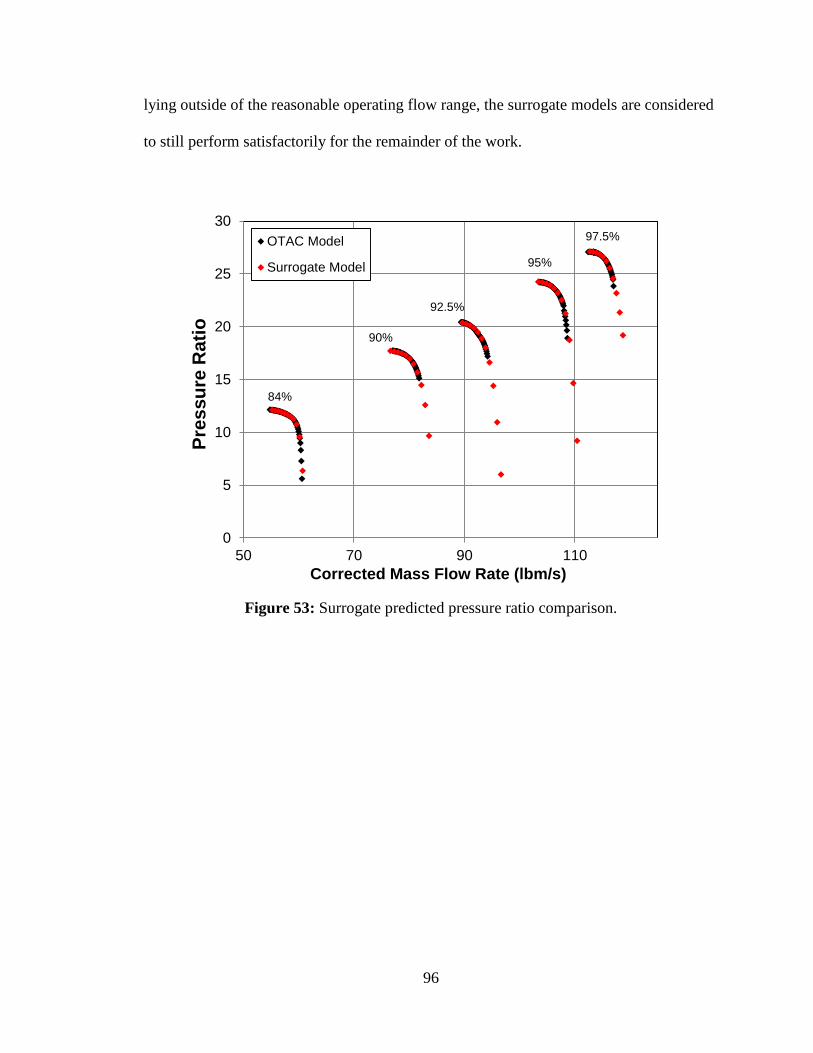
96

lying outside of the reasonable operating flow range, the surrogate models are considered

to still perform satisfactorily for the remainder of the work.

Figure 53: Surrogate predicted pressure ratio comparison.

0

5

10

15

20

25

30

50 70 90 110

Pre

ss

ure

Ra

tio


OTAC Model

Surrogate Model

84%

90%

92.5%

95%

97.5%

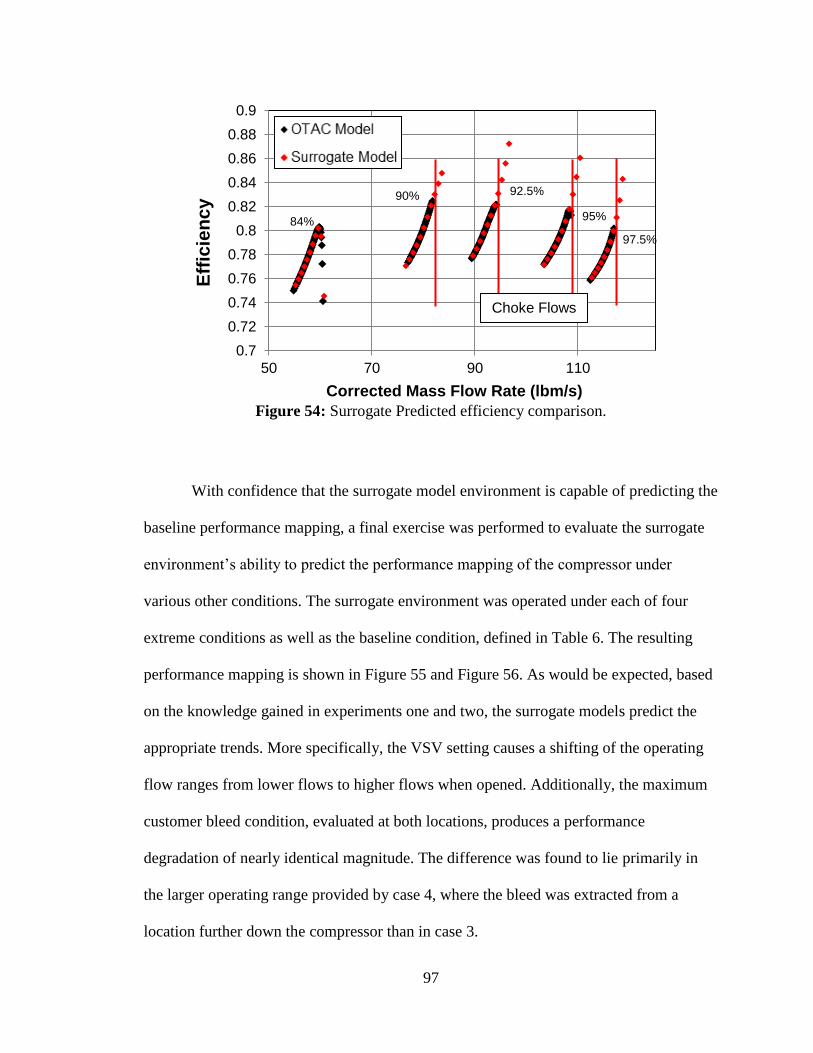
97

Figure 54: Surrogate Predicted efficiency comparison.

With confidence that the surrogate model environment is capable of predicting the

baseline performance mapping, a final exercise was performed to evaluate the surrogate

environment’s ability to predict the performance mapping of the compressor under

various other conditions. The surrogate environment was operated under each of four

extreme conditions as well as the baseline condition, defined in Table 6. The resulting

performance mapping is shown in Figure 55 and Figure 56. As would be expected, based

on the knowledge gained in experiments one and two, the surrogate models predict the

appropriate trends. More specifically, the VSV setting causes a shifting of the operating

flow ranges from lower flows to higher flows when opened. Additionally, the maximum

customer bleed condition, evaluated at both locations, produces a performance

degradation of nearly identical magnitude. The difference was found to lie primarily in

the larger operating range provided by case 4, where the bleed was extracted from a

location further down the compressor than in case 3.

0.7

0.72

0.74

0.76

0.78

0.8

0.82

0.84

0.86

0.88

0.9

50 70 90 110

Eff

icie

nc

y


Choke Flows

84%

90% 92.5%

95%

97.5%

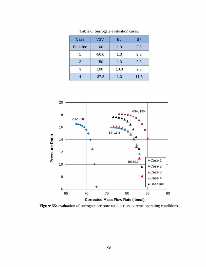
98

Table 6: Surrogate evaluation cases.

Case VSV B5 B7

Baseline 100 1.3 2.3

1 -50.0 1.3 2.3

2 150 1.3 2.3

3 100 10.3 2.3

4 -37.8 1.3 11.3

Figure 55: evaluation of surrogate pressure ratio across extreme operating conditions.

6

8

10

12

14

16

18

20

65 70 75 80 85 90

Pre

ss

ure

Rati

o


Case 1

Case 2

Case 3

Case 4

Baseline

VSV: -50

B7: 11.3

B5:10.3

VSV: 150

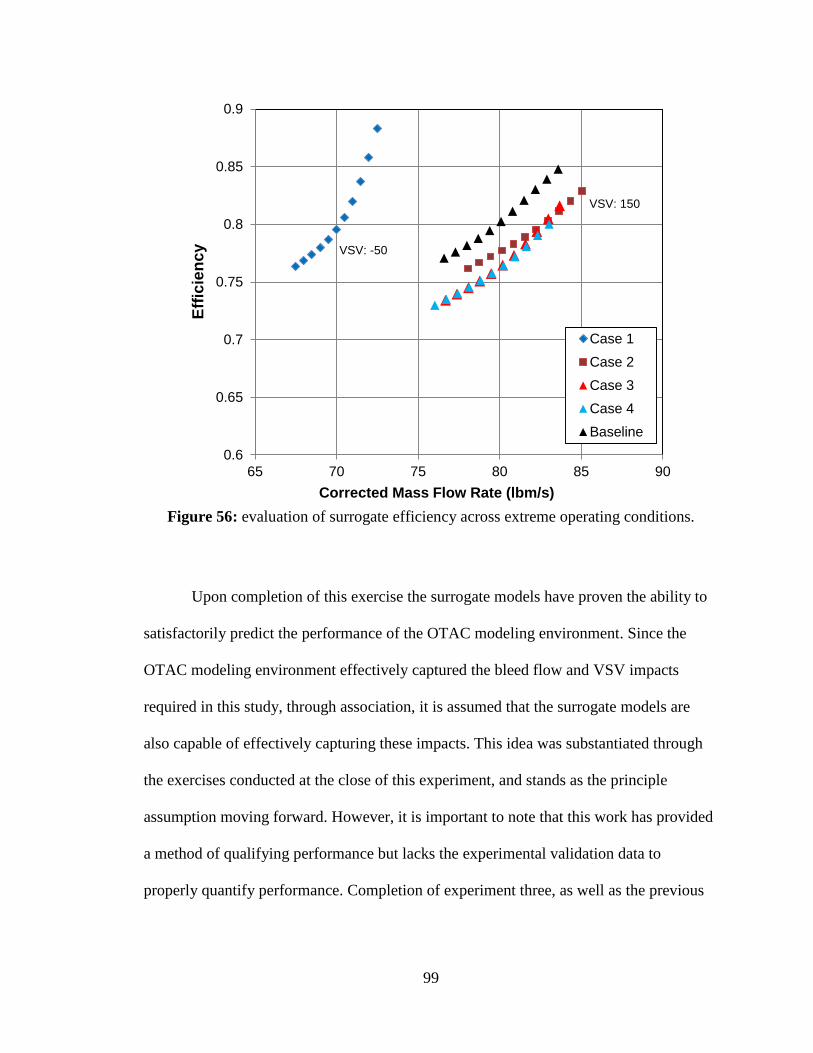
99

Figure 56: evaluation of surrogate efficiency across extreme operating conditions.

Upon completion of this exercise the surrogate models have proven the ability to

satisfactorily predict the performance of the OTAC modeling environment. Since the

OTAC modeling environment effectively captured the bleed flow and VSV impacts

required in this study, through association, it is assumed that the surrogate models are

also capable of effectively capturing these impacts. This idea was substantiated through

the exercises conducted at the close of this experiment, and stands as the principle

assumption moving forward. However, it is important to note that this work has provided

a method of qualifying performance but lacks the experimental validation data to

properly quantify performance. Completion of experiment three, as well as the previous

0.6

0.65

0.7

0.75

0.8

0.85

0.9

65 70 75 80 85 90

Eff

icie

ncy


Case 1

Case 2

Case 3

Case 4

Baseline

VSV: -50

VSV: 150

100

two experiments, has yielded a powerful tool capable of answering the first research

question in a quick and effective manner:



Experiment 4

Experiments one, two, and three served to sufficiently capture and quantify the

compressor level impacts, as well as to deliver the capability to quickly quantify these

impacts parametrically, and independently of the original compressor analysis tool. The

final experiment was designed to answer the second research question:


compressor design?

Experiment four was designed to answer this question, and to do so, required the

completion of the following three tasks:

1. Construct an engine cycle analysis using the baseline full compressor mapping

constructed at the normal conditions of bleed flow and VSV orientation.

2. Include the RSE as an additional object in line with the base compressor object to

replace the performance outputs from this base compressor object with the RSE

outputs, based on an extra set of bleed and VSV inputs provided by the user. The

RSE will solve for a new mapping which will replace the existing mapping.

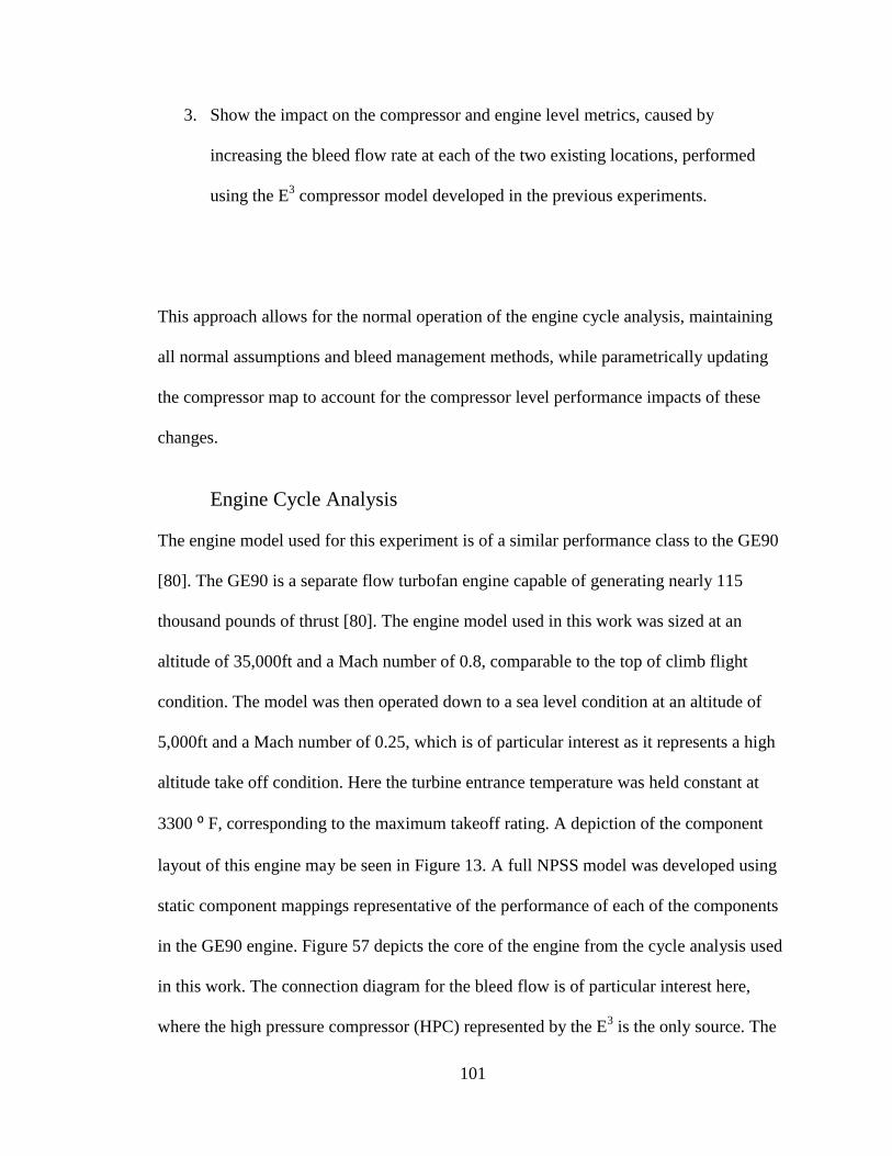
101

3. Show the impact on the compressor and engine level metrics, caused by

increasing the bleed flow rate at each of the two existing locations, performed

using the E3 compressor model developed in the previous experiments.

This approach allows for the normal operation of the engine cycle analysis, maintaining

all normal assumptions and bleed management methods, while parametrically updating

the compressor map to account for the compressor level performance impacts of these

changes.

Engine Cycle Analysis

The engine model used for this experiment is of a similar performance class to the GE90

[80]. The GE90 is a separate flow turbofan engine capable of generating nearly 115

thousand pounds of thrust [80]. The engine model used in this work was sized at an

altitude of 35,000ft and a Mach number of 0.8, comparable to the top of climb flight

condition. The model was then operated down to a sea level condition at an altitude of

5,000ft and a Mach number of 0.25, which is of particular interest as it represents a high

altitude take off condition. Here the turbine entrance temperature was held constant at

3300 ⁰ F, corresponding to the maximum takeoff rating. A depiction of the component

layout of this engine may be seen in Figure 13. A full NPSS model was developed using

static component mappings representative of the performance of each of the components

in the GE90 engine. Figure 57 depicts the core of the engine from the cycle analysis used

in this work. The connection diagram for the bleed flow is of particular interest here,

where the high pressure compressor (HPC) represented by the E3 is the only source. The

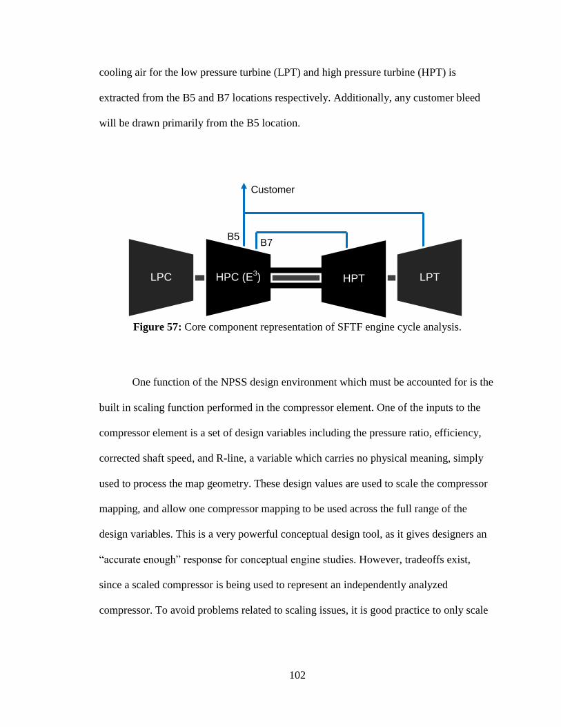
102

cooling air for the low pressure turbine (LPT) and high pressure turbine (HPT) is

extracted from the B5 and B7 locations respectively. Additionally, any customer bleed

will be drawn primarily from the B5 location.

Figure 57: Core component representation of SFTF engine cycle analysis.

One function of the NPSS design environment which must be accounted for is the

built in scaling function performed in the compressor element. One of the inputs to the

compressor element is a set of design variables including the pressure ratio, efficiency,

corrected shaft speed, and R-line, a variable which carries no physical meaning, simply

used to process the map geometry. These design values are used to scale the compressor

mapping, and allow one compressor mapping to be used across the full range of the

design variables. This is a very powerful conceptual design tool, as it gives designers an

“accurate enough” response for conceptual engine studies. However, tradeoffs exist,

since a scaled compressor is being used to represent an independently analyzed

compressor. To avoid problems related to scaling issues, it is good practice to only scale

HPC (E3) LPC HPT LPT

B5 B7

Customer

103

a compressor mapping a small amount from the original performance and operating

range.

RSE Integration

The second piece of experiment four calls for the integration of the surrogate

environment developed in experiment three into the engine cycle analysis constructed in

the previous part of this experiment. Fortunately, the original development of the

surrogate environment was completed in the NPSS modeling system, so the remaining

challenge was determining a way to successfully update the existing HPC map with the

responses predicted by the surrogate models. The first approach to updating the HPC map

was simple: replace all of the static numeric values in the mapping with variables which

could be linked to the solutions of the surrogate models. Unfortunately, the compressor

mapping element manages its performance mapping data in a collection of tables, and

NPSS will not allow the tables to contain variables. To circumnavigate this, the main

operating file for the engine cycle analysis, which also contains the surrogate

environment, was amended to allow for the creation of a replacement compressor object

each time the cycle analysis was operated. This replacement compressor object is an

exact replica of the existing object, only containing the updated mappings which are

recalculated by the surrogate models at the beginning of every cycle analysis, and saved

under a different name. Additionally, the logic was added to enable the user to toggle this

process on or off, depending on whether or not the designer wishes to utilize updated

maps or the existing static map. This process is depicted by Figure 58.

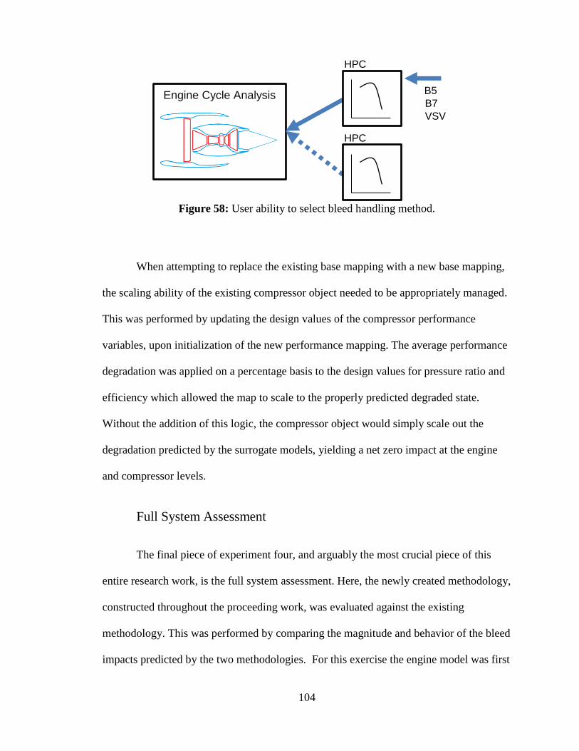
104

Figure 58: User ability to select bleed handling method.

When attempting to replace the existing base mapping with a new base mapping,

the scaling ability of the existing compressor object needed to be appropriately managed.

This was performed by updating the design values of the compressor performance

variables, upon initialization of the new performance mapping. The average performance

degradation was applied on a percentage basis to the design values for pressure ratio and

efficiency which allowed the map to scale to the properly predicted degraded state.

Without the addition of this logic, the compressor object would simply scale out the

degradation predicted by the surrogate models, yielding a net zero impact at the engine

and compressor levels.

Full System Assessment

The final piece of experiment four, and arguably the most crucial piece of this

entire research work, is the full system assessment. Here, the newly created methodology,

constructed throughout the proceeding work, was evaluated against the existing

methodology. This was performed by comparing the magnitude and behavior of the bleed

impacts predicted by the two methodologies. For this exercise the engine model was first

B5

B7 Engine Cycle Analysis

VSV

HPC

HPC

105

evaluated, case one, using the E3 B1 performance mapping, under the design bleed and

VSV settings, where the VSV orientation was set to 100% open, and 1.3% and 2.3% of

the previous stage discharge flow was extracted just after the 5th

(B5) and 7th

(B7) stage

stators, respectively. Following this, case two, the traditional bleed handling methodology

was applied, where the same performance mapping as in the previous case was used, but

an additional customer bleed air was added, at a magnitude of 5% of the previous stage

discharge flow, extracted from the B5 location, while the cooling bleed and VSV settings

remained the same as before. The final case, case three, was operated under the exact

settings as case two, but with the replacement of the static map with an updated map,

constructed by the surrogate models to account for the additional customer bleed.

It is expected that the variable map bleed management will predict a greater

performance and operability impact than that which would be predicted by the traditional

bleed management method. In order to assess this hypothesis, it is important to evaluate

the impact that is predicted by the traditional method of bleed management (case two)

compared to case one, where no bleed flow was extracted. The compressor level impact

that the additional bleed flow extraction had on both the pressure ratio and efficiency may

be seen in Figure 59 and Figure 60, respectively. Seen here, the base compressor,

identical for both cases, has been mass flow scaled to meet the additional flow

requirements of the engine system. The operating line shifts to a higher flow range as

well, once again due to the additional flow requirements of the system. The system is

requiring more flow because it is working to maintain the same thrust, which is

proportion to the mass flow through the engine, before and after the addition of the

106

customer bleed requirement. No compressor level performance degradation is observable

in the case of the fixed map bleed handling.

Figure 59: Pressure ratio mapping impact with the addition of bleed.

5

10

15

20

25

40 50 60 70 80 90 100 110

Pre

ss

ure

Rati

o


Case 1

Case 2

Case 1 Opline

Case 2 Opline

97.5%

95%

92.5%

90%

84%

107

Figure 60: Efficiency mapping impact with the addition of bleed.

In order to evaluate the difference in the performance predictions produced by the

two bleed handling methods, the performance mappings from case two and case three are

shown for pressure ratio and efficiency in Figure 61 and Figure 62 respectively. The first

clear impact was found in the compressor performance. As would be expected from all of

the proceeding work, the compressor performance degradation is apparent, where the

predicted pressure ratio and efficiency are much lower than in the case where the

mapping neglects the bleed flow impacts. Additionally, the operating line of the

compressor is negatively impacted. The operating line determined under the variable map

bleed handling method utilized in case three predicts both a performance degradation,

which should be expected to manifest itself at the engine level, as well as a shifting to a

higher operating flow range due to the additional corrected shaft speed and corrected

flow requirements for achieving the desired pressure increase. Based off of these

0.7

0.72

0.74

0.76

0.78

0.8

0.82

0.84

0.86

0.88

0.9

40 50 60 70 80 90 100 110

Pre

ss

ure

Rati

o


Case 1

Case 2

Case 1 Opline

Case 2 Opline

84%

90%

92.5%

95%

97.5%

108

mappings, the traditional method for handling bleed flow is under-predicting the

performance impact from bleed flow extraction at the compressor level.

Figure 61: Pressure ratio performance predictions from both bleed handling methods.

5.0

10.0

15.0

20.0

25.0

40.0 50.0 60.0 70.0 80.0 90.0 100.0 110.0

Pre

ss

ure

Rati

o


Case 2

Case 3

Case 2 Opline

Case 3 Opline

97.5%

95%

92.5%

90%

84%

109

Figure 62: Efficiency performance predictions from both bleed handling methods.

Now that the compressor level impacts have been evaluated, it is of particular

interest to assess these impacts at the engine level, with the same attention to the

variations in predicted performance produced by the two bleed management methods

explored here. The thrust specific fuel consumption (TSFC) introduced before, was the

metric of interest used to compare these impacts on the predicted engine level

performance. A comparison of the three cases, evaluated at the same conditions as before,

is shown in Figure 63. Case one exhibits the lowest TSFC, which is to be expected since

there is no bleed flow extraction present. Following this, case two exhibits a higher

TSFC, which should once again be expected. Based on the unaffected compressor level

performance between case one and case two, it is reasonable to assume that any impact

0.700

0.720

0.740

0.760

0.780

0.800

0.820

0.840

0.860

0.880

0.900

45.0 55.0 65.0 75.0 85.0 95.0 105.0 115.0

Eff

icie

ncy


Case 1

Case 3

Case 1 Opline

Case 3 Opline

84%

90% 92.5%

95% 97.5%

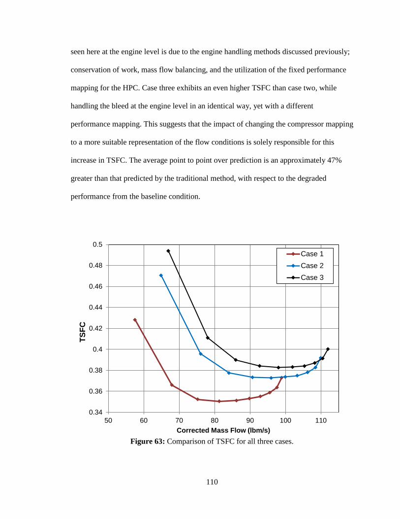
110

seen here at the engine level is due to the engine handling methods discussed previously;

conservation of work, mass flow balancing, and the utilization of the fixed performance

mapping for the HPC. Case three exhibits an even higher TSFC than case two, while

handling the bleed at the engine level in an identical way, yet with a different

performance mapping. This suggests that the impact of changing the compressor mapping

to a more suitable representation of the flow conditions is solely responsible for this

increase in TSFC. The average point to point over prediction is an approximately 47%

greater than that predicted by the traditional method, with respect to the degraded

performance from the baseline condition.

Figure 63: Comparison of TSFC for all three cases.

0.34

0.36

0.38

0.4

0.42

0.44

0.46

0.48

0.5

50 60 70 80 90 100 110

TS

FC


Case 1

Case 2

Case 3

111

The final assessment was conducted to evaluate the predicted engine level

operability impact. Generated from the same testing conducted before, the stall margin

across the operating line performed is plotted for each of the three cases, in figure 64.

Here it is apparent that the cases where customer bleed is applied manage to achieve a

larger stall margin than in the baseline case, which is to be expected. Of greater

importance here, is the fact that the newly developed bleed handling case predicts a

higher stall margin than in the traditional bleed handling case. The positive impact of this

is that engine designs using the traditional method would be more conservative.

However, a potentially negative impact may be found where engine designers make

unnecessary compromises to meet overly conservative, and potentially incorrectly

predicted stall margins. This aside, these results are in line with what would be expected,

based on the former analyses of this experiment and the more stringent manner with

which the new methodology handles bleed.

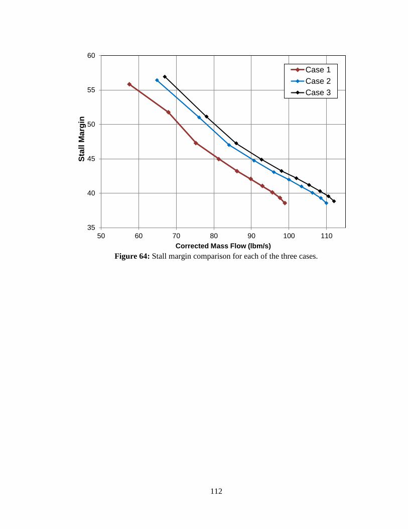
112

Figure 64: Stall margin comparison for each of the three cases.

35

40

45

50

55

60

50 60 70 80 90 100 110

Sta

ll M

arg

in


Case 1

Case 2

Case 3

113

CHAPTER V: CONCLUSIONS

The commercial aviation industry is currently facing the challenge of reducing

fuel consumption for the next generation of aircraft. The most likely approach to

accomplishing this will be through the pursuit of higher bypass ratio engines. Since the

size of the fan at the front of the engine is constrained to nearly its current size, this

increase in bypass ratio must be accomplished through a decrease in the core size. This

reduced core size, and associated reduced air flow, makes bleed flow extracted from the

engine more costly than before, necessitating a way to measure the impacts of this

extraction in the engine conceptual design environment.

Problem Statement: In the conceptual design phase, how does one determine the

minimum core size to meet compressor performance and operability while accounting for

subsystem bleed requirements?

Research Questions

Two research questions were developed, which upon successful completion,

would provide a valid solution to the above stated problem. The completed work

revolved around answering these questions as effectively as necessary for the scope of

the problem statement.



114

This work answered this question by means of a three part approach, the platform

for which being a multi-stream meanline modeling environment. The first piece of this

approach called for the sufficient modeling of the variable stator vanes (VSVs), as they

carry a large impact on the compressor flow conditioning and operability management.

This was completed by amending the mechanism for maintaining blade metal angles in

the modeling environment to appropriately account for the geometric change caused by

rotating the blades. A full model was created with the inclusion of these changes and

compared well against experimental test data.

The second piece of the approach required the prediction of bleed impacts at the

compressor level, and was manifested through the same modeling environment used to

model the VSVs. A simple modeling structure was developed to utilize the multiple

streamline characteristic of the model. This structure allowed the streamlines to be

systematically separated, before being reconditioned or removed, to directly simulate the

mechanism of bleed flow extraction in the compressor. This structure was implemented

across each of the streams with success, and this full span extraction structure was

included in the full compressor model from before. The resultant model exhibited all of

the expected trends, and fared well to sufficiently capture the impacts of bleed.

Upon completion of the first two pieces of this approach, the first research

question can be successfully answered. However, the answer requires the operation of the

compressor model developed before, which is computationally and time expensive,

requiring up to an hour to develop a single full compressor mapping. Part three

intentioned to develop a rapid approach to producing the response predictions provided

by parts one and two. This was proven to be accomplishable through the implementation

115

of response surface equations (RSEs), which are mathematical models capable of

replacing the modeling environment required in the first two pieces. This method of

replacement required a large amount of strategically gathered data from the modeling

environment, specifically a design of experiments (DoE) consisting of approximately

11,000 cases. The collection of RSEs was implemented into a modeling environment,

where it was used to produce performance predictions for comparison to the original

modeling environment prediction. Here the surrogate environment performed well,

successfully defining a way to answer the first research question in a time and

computationally inexpensive way. This step was necessary for engine level analyses,

where rapid response times at the component level are essential for conceptual design

decisions.

The combination of these three pieces effectively yielded a simple environment

which leveraged fifteen equations to replace a massive amount of data. Without this

capability, the design space exploration would be too cumbersome to be practical at the

engine level, possibly disallowing designers from recognizing more preferable design

solutions. The second research question was designed to take the information gathered in

the successful fulfillment of the first question and to apply it at the engine level:


compressor design?

The traditional method for answering this question requires the handling of bleed

at the engine system level, with no regard for the lower level impacts of the compressor

116

within the system. It assumes that the performance of the compressor is so negligibly

impacted by bleed, that a static performance mapping is sufficient for capturing the

engine level impacts. On the contrary, this work challenges this method by proposing a

more stringent answer to the question.

This work answered this question by integrating the surrogate environment,

developed before, into an engine modeling environment capable of isolating and

evaluating the prediction disparity between the existing and developed bleed handling

methodologies. This engine modeling environment took the form of a thermodynamic

cycle analysis of a separate flow turbofan engine (SFTF). The integration of the surrogate

environment allowed for the rapid updating of the previously static compressor

performance mappings in the engine modeling environment based on user specified bleed

and VSV settings. This “zooming” capability allows engine designers to evaluate engine

level impacts from sub-engine level component configurations.

Engine level studies reveled a performance trend where the newly developed

bleed handling method predicted a consistently more negative response then that

predicted by the traditional method. This was evidenced by a greater TSFC prediction, as

well as by a predicted operating line which displayed a need for the compressor to work

harder to accomplish the same engine level conditions, produced by the newly developed

methodology. With regards to operability, the newly developed methodology predicted a

consistently larger stall margin than the traditional method.

The main take away from the totality of this research is the existence of the

discrepancy between the two engine level bleed handling methods. The traditional

method operates on the assumption that the engine sub-level compressor performance

117

impacts due to the introduction of bleed are negligible. This is clearly not the case. The

first portion of this research served to provide a qualification for the extent to which

bleed impacts the compressor level, and yielded significant impacts. The final portion of

this research applied this qualification at the engine level, and found that the significant

engine sub-level (compressor) impacts propagated up to the engine level and remained

significant. This result necessitates a more stringent handling of bleed at the engine level

than the traditional method provides, and the results of this research suggest that the

newly developed methodology provides an effective means to further the realization of

this goal.

The problem statement fueling this research required a means to assess the

minimum core size to meet the performance and operability requirements of the

compressor, specifically in the conceptual design phase. This may be currently

accomplished through the engine cycle analysis, where engine performance drives the

compressor level requirements. Additionally, the problem statement required the

determination of the minimum core size in the presence of bleed. To provide a solution,

the engine level analysis was amended to allow the bleed driven impacts at the

compressor level to propagate up to the engine. This capability to assess both the

compressor and engine level impacts of bleed in an interactive way, has given engine

designers the ability to determine the minimum core size to meet compressor

performance and operability while accounting for subsystem bleed requirements.

118

Recommendations

This work has introduced a very positive methodology for capturing the

compressor and engine level impacts, with respect to both performance and operability,

from bleed flow extraction. However, there are multiple pieces of this work which upon

further improvement would greatly benefit future work. The first of these includes the

introduction of point to point solving in OTAC, with respect to pattern free design space

exploration. OTAC’s lack of capability to operate on a pattern free basis has greatly

limited the abilities of various DoEs to encompass the design space. Additionally, it

would be a great benefit to automate the mapping construction process within OTAC.

The current method requires an initial estimate of design flow which must be fairly close

the converged design flow, making mapping construction a very iterative and

cumbersome task. It would also be wise to implement a stall and choke model into the

OTAC modeling environment. This would allow for the removal of the “offset flow”,

which is fairly subjective in nature, and would also increase the accuracy of the stall flow

surrogate models, as more successfully converged stall flows would be included in their

formation. Finally, it would be of great use to the motivation fueling this research, and

any subsequent work to experimentally validate the bleed flow extraction model

developed here. The physics of the problem is well captured in the provided solution, but

validation would enable a greater utilization of the developed methodology.

119

APPENDIX A: ERROR AND UNCERTAINTY ANALYSES Point to Point error for compressor point:

𝐸𝑟𝑟𝑜𝑟 (%) = (𝑃𝑜𝑖𝑛𝑡𝑀𝑜𝑑𝑒𝑙 − 𝑃𝑜𝑖𝑛𝑡𝐸𝑚𝑝𝑖𝑟𝑖𝑐𝑎𝑙

𝑃𝑜𝑖𝑛𝑡𝐸𝑚𝑝𝑖𝑟𝑖𝑐𝑎𝑙) ∗ 100

Total average point to point error:

𝑓𝑜𝑟 𝑛 = 1 𝑡𝑜 𝑛 … 𝐴𝑣𝑒𝑟𝑎𝑔𝑒 𝐸𝑟𝑟𝑜𝑟 (%) = ∑(𝑝𝑜𝑖𝑛𝑡 𝑡𝑜 𝑝𝑜𝑖𝑛𝑡 𝑒𝑟𝑟𝑜𝑟)

𝑛

Mean of a statistical distribution: The average

�̅� = ∑ 𝑥𝑖𝑛

Standard Deviation of a statistical distribution: The square root of the variance. (Variance: defines

the spread of a data set)

𝑆 = √∑(𝑥 − �̅�)2

𝑛 − 1

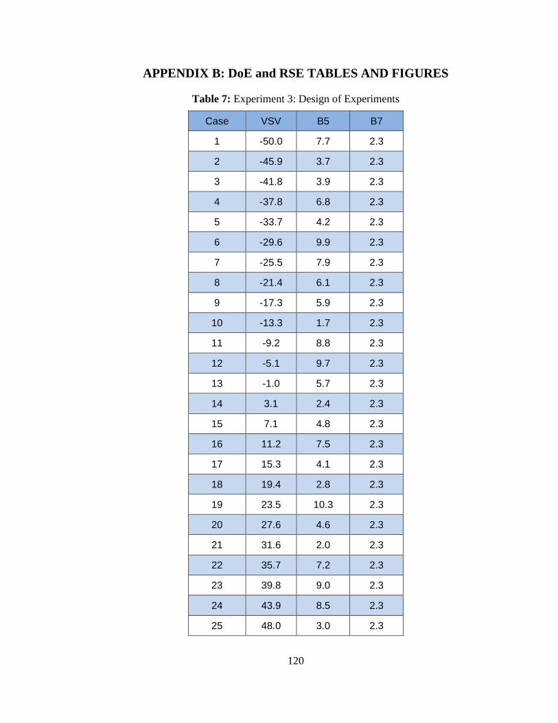
120

APPENDIX B: DoE and RSE TABLES AND FIGURES

Table 7: Experiment 3: Design of Experiments

Case VSV B5 B7

1 -50.0 7.7 2.3

2 -45.9 3.7 2.3

3 -41.8 3.9 2.3

4 -37.8 6.8 2.3

5 -33.7 4.2 2.3

6 -29.6 9.9 2.3

7 -25.5 7.9 2.3

8 -21.4 6.1 2.3

9 -17.3 5.9 2.3

10 -13.3 1.7 2.3

11 -9.2 8.8 2.3

12 -5.1 9.7 2.3

13 -1.0 5.7 2.3

14 3.1 2.4 2.3

15 7.1 4.8 2.3

16 11.2 7.5 2.3

17 15.3 4.1 2.3

18 19.4 2.8 2.3

19 23.5 10.3 2.3

20 27.6 4.6 2.3

21 31.6 2.0 2.3

22 35.7 7.2 2.3

23 39.8 9.0 2.3

24 43.9 8.5 2.3

25 48.0 3.0 2.3

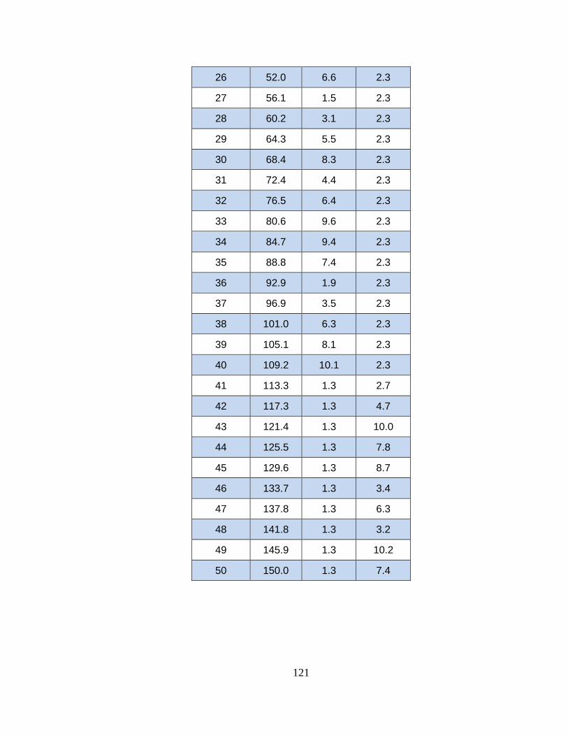
121

26 52.0 6.6 2.3

27 56.1 1.5 2.3

28 60.2 3.1 2.3

29 64.3 5.5 2.3

30 68.4 8.3 2.3

31 72.4 4.4 2.3

32 76.5 6.4 2.3

33 80.6 9.6 2.3

34 84.7 9.4 2.3

35 88.8 7.4 2.3

36 92.9 1.9 2.3

37 96.9 3.5 2.3

38 101.0 6.3 2.3

39 105.1 8.1 2.3

40 109.2 10.1 2.3

41 113.3 1.3 2.7

42 117.3 1.3 4.7

43 121.4 1.3 10.0

44 125.5 1.3 7.8

45 129.6 1.3 8.7

46 133.7 1.3 3.4

47 137.8 1.3 6.3

48 141.8 1.3 3.2

49 145.9 1.3 10.2

50 150.0 1.3 7.4

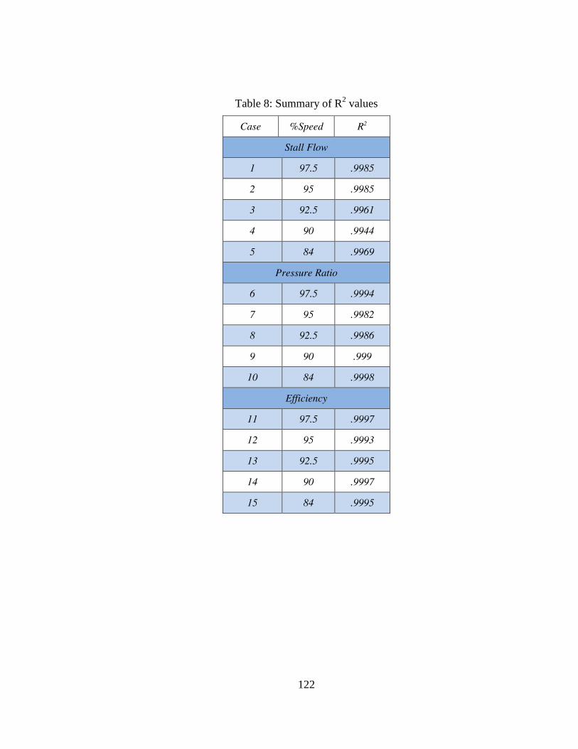
122

Table 8: Summary of R2 values

Case %Speed R2

Stall Flow

1 97.5 .9985

2 95 .9985

3 92.5 .9961

4 90 .9944

5 84 .9969

Pressure Ratio

6 97.5 .9994

7 95 .9982

8 92.5 .9986

9 90 .999

10 84 .9998

Efficiency

11 97.5 .9997

12 95 .9993

13 92.5 .9995

14 90 .9997

15 84 .9995

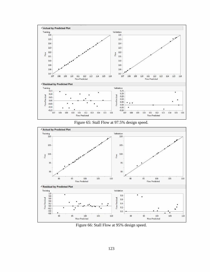
123

Figure 65: Stall Flow at 97.5% design speed.

Figure 66: Stall Flow at 95% design speed.

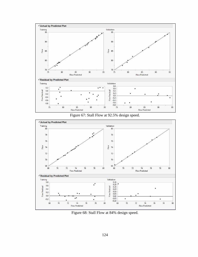
124

Figure 67: Stall Flow at 92.5% design speed.


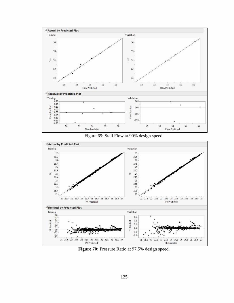
125


Figure 70: Pressure Ratio at 97.5% design speed.

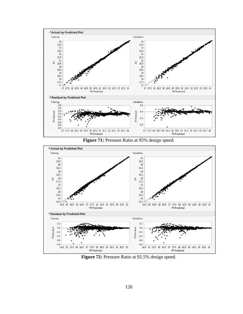
126

Figure 71: Pressure Ratio at 95% design speed.

Figure 72: Pressure Ratio at 92.5% design speed.

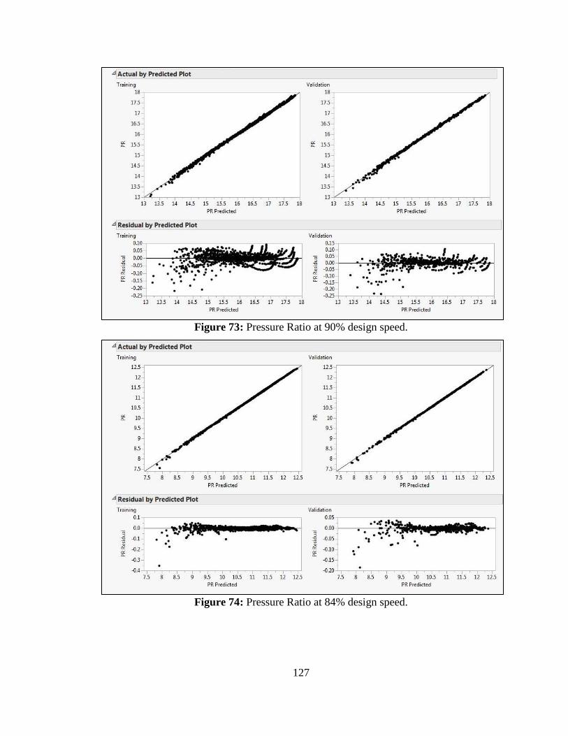
127



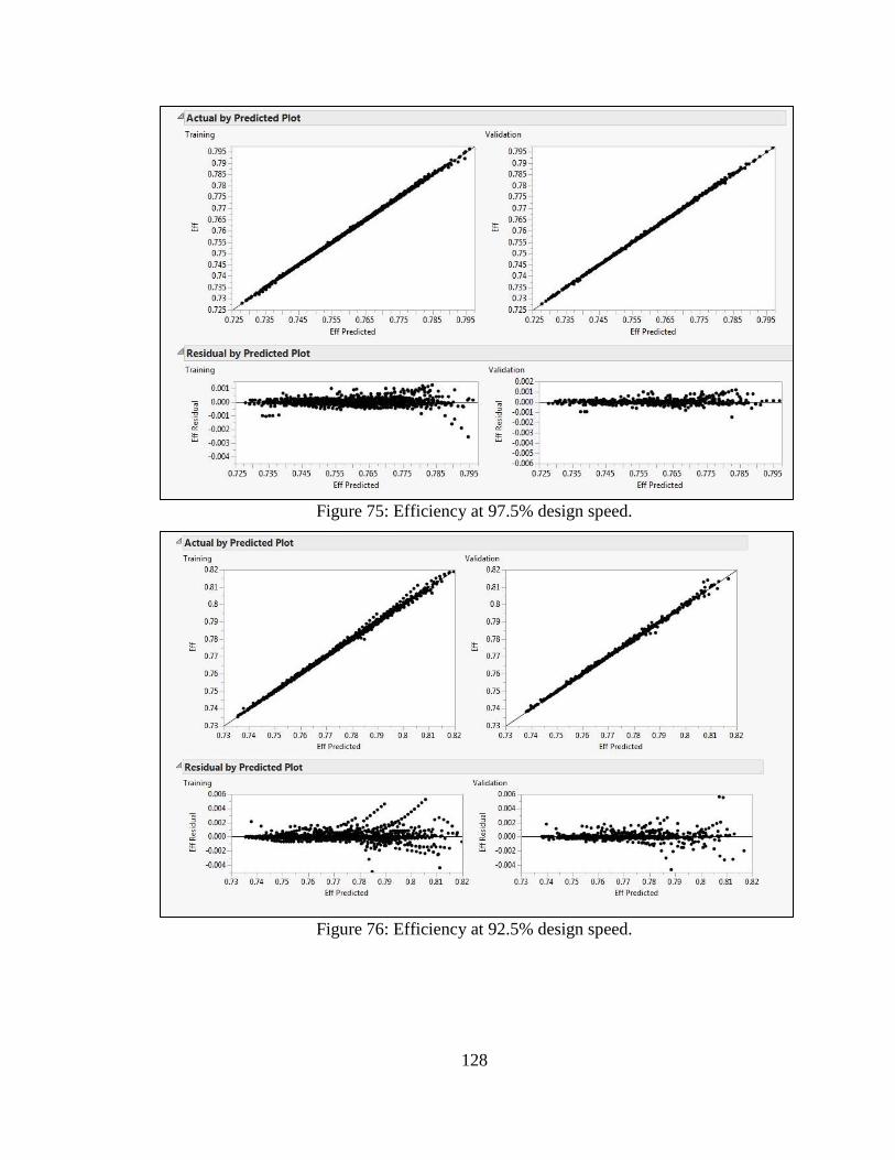
128

Figure 75: Efficiency at 97.5% design speed.

Figure 76: Efficiency at 92.5% design speed.

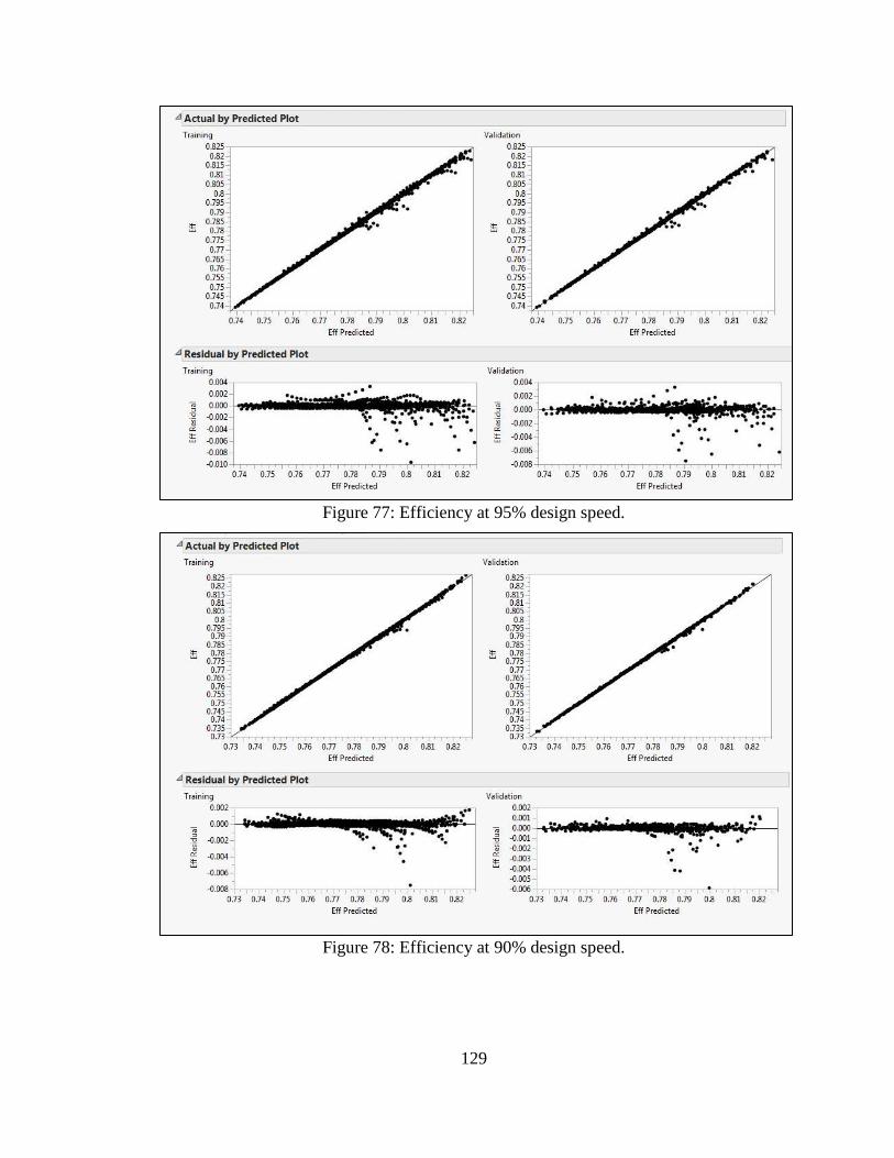
129

Figure 77: Efficiency at 95% design speed.


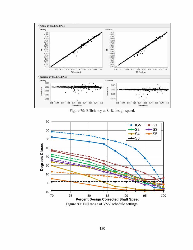
130


Figure 80: Full range of VSV schedule settings.

-10

0

10

20

30

40

50

60

70

70 75 80 85 90 95 100

Deg

ree

s C

los

ed

Percent Design Corrected Shaft Speed

IGV S1S2 S3S4 S5S6

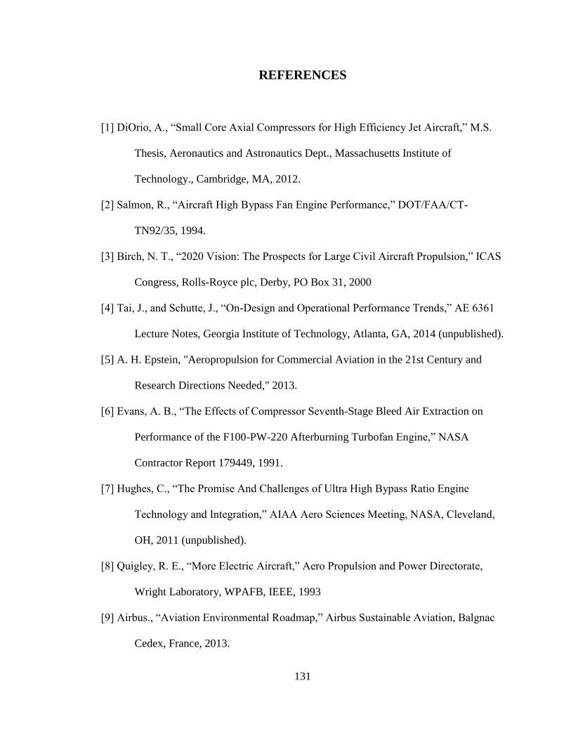
131

REFERENCES

[1] DiOrio, A., “Small Core Axial Compressors for High Efficiency Jet Aircraft,” M.S.

Thesis, Aeronautics and Astronautics Dept., Massachusetts Institute of

Technology., Cambridge, MA, 2012.

[2] Salmon, R., “Aircraft High Bypass Fan Engine Performance,” DOT/FAA/CT-

TN92/35, 1994.

[3] Birch, N. T., “2020 Vision: The Prospects for Large Civil Aircraft Propulsion,” ICAS

Congress, Rolls-Royce plc, Derby, PO Box 31, 2000

[4] Tai, J., and Schutte, J., “On-Design and Operational Performance Trends,” AE 6361

Lecture Notes, Georgia Institute of Technology, Atlanta, GA, 2014 (unpublished).

[5] A. H. Epstein, "Aeropropulsion for Commercial Aviation in the 21st Century and

Research Directions Needed," 2013.

[6] Evans, A. B., “The Effects of Compressor Seventh-Stage Bleed Air Extraction on

Performance of the F100-PW-220 Afterburning Turbofan Engine,” NASA

Contractor Report 179449, 1991.

[7] Hughes, C., “The Promise And Challenges of Ultra High Bypass Ratio Engine

Technology and Integration,” AIAA Aero Sciences Meeting, NASA, Cleveland,

OH, 2011 (unpublished).

[8] Quigley, R. E., “More Electric Aircraft,” Aero Propulsion and Power Directorate,

Wright Laboratory, WPAFB, IEEE, 1993

[9] Airbus., “Aviation Environmental Roadmap,” Airbus Sustainable Aviation, Balgnac

Cedex, France, 2013.

132

[10] National Aeronautics and Space Administration., “Energy, Efficiency, and

Emissions,” NF200908488HQ, 2009.

[11] International Air Transport Association., “Operational Fuel Efficiency,” IATA

Programs, URL: http://www.iata.org/whatwedo/ops-infra/Pages/fuel-

efficiency.aspx [cited 3 June 2014].

[12] Mavris, D.N., DeLaurentis, D.A., Bandte, O., Hale, M.A., "A Stochastic Approach

to Multi-disciplinary Aircraft Analysis and Design", AIAA 98-0912.

[13] Mavris, D., “A “Paradigm Shift” in Complex System Design,” AE 6373 Lecture

Notes, Georgia Institute of Technology, Atlanta, GA, 2014 (unpublished).

[14] Mavris, D., “Requirements Analysis,” AE 6343 Lecture Notes, Georgia Institute of

Technology, Atlanta, GA, 2011 (unpublished).

[15] N. U. Rahman, J. F. Whidborne, “A numerical investigation into the effect of engine

bleed on performance of a single-spool turbojet engine," Journal of Aerospace

Engineering, Volume 222, Number 7, 939-949, 2008.

[16] Turner, M. G., Reed, J. A., Ryder, R., Veres, J. P., “Multi-Fidelity Simulation of a

Turbofan Engine With Results Zoomed Into Mini-Maps for a Zero-D Cycle

Simulation,” NASA/TM - 2004-213076, 2004.

[17] Reed, J. A., Turner, M. G., Norris, A., Veres, J. P., “Towards an Automated Full-

Turbofan Engine Numerical Simulation,” NASA/TM - 2003-212494, 2003.

[18] Pachidis, V., Pilidis, P., Texeira, J., Templalexis, I., “A Comparison of Component

Zooming Simulation Strategies Using Streamline Curvature,” Journal of

Aerospace Engineering, Volume 221 Part G, 2007.

133

[19] Pachidis, V., Pilidis, J., Templalexis, I., Barbosa, J. B., Nantua, N., “A De-Coupled

Approach to Component High-Fidelity Analysis Using Computational Fluid

Dynamics,” Journal of Aerospace Engineering, Volume 221 Part G, 2007.

[20] Pachidis, V., Pilidis, J., Templalexis, I., Guindeuil, G., Kalfas, A., “A Partially

Integrated Approach to Component Zooming Using Computational Fluid

Dynamics,” ASME Turbo Expo 2005, GT2005-68457, 2005.

[21] Pachidis, V., Pilidis, J., Templalexis, I., Talhouarn, F., Kalfas, A., “A Fully

Integrated Approach to Component Zooming Using Computational Fluid

Dynamics,” ASME Turbo Expo 2005, GT2005-68457, 2005.

[22] Tai, J., and Schutte, J., “Off-Design Introduction,” AE 6361 Lecture Notes, Georgia

Institute of Technology, Atlanta, GA, 2014 (unpublished).

[23] Cengel, Y., Turner, R., Fundamentals of Thermal-Fluid Sciences, 2nd

ed., McGraw

Hill, New York, 2005, Chaps. 8.

[24] Schobeiri, M., Turbomachinery Flow Physics and Dynamic Performance, 1st ed.,

Springer, Verlag Berlin Heidelberg, 2004, Chaps. nnnnnnnnnn.

[25] Aungier, R., Axial Flow Compressors, A Strategy for Aerodynamic Design and

Analysis, 1st ed., ASME Press, New York, 2003, Chaps. nnnnnnn.

[26] Cohen, H., Rogers, G.F.C., Saravanamuttoo, H.I.H., Gas Turbine Theory, 4th

ed.,

Longman House, Harlow, 1996, Chaps. nnnnnnn.

134

[27] Cumpsty, N., Jet Propulsion, A Simple Guide to the Aerodynamic and

Thermodynamic Design and Performance of Jet Engines, 2nd

ed., Cambridge

University Press, New York, 2003, Chaps. 11.

[28] Moeckel, C., Multi-Stage Axial Compressor, Photo, MIT Gas Turbine Laboratory,

MA, 2006

[29] Follen, G., auBuchon, M., “Numerical Zooming Between a NPSS Engine System

Simulation and a One-Dimensional High Compressor Analysis Code,”

NASA/TM - 2000-209913, 2000.

[30] Tai, J., and Schutte, J., “Thermodynamic Cycle Analysis – On Design,” AE 6361


[31] Annual Crude oil and Jet Fuel Prices. (2014, January 1). . Retrieved June 12, 2014,

from http://www.airlines.org/Pages/Annual-Crude-Oil-and-Jet-Fuel-Prices.aspx

[32] Fuel Price Analysis. (2014, January 1). . Retrieved June 12, 2014, from

http://www.iata.org/publications/economics/fuel-monitor/Pages/price-

analysis.aspx

[33] “Aviation and Emissions, A Primer,” Federal Aviation Administration, Office of

Environment and Energy, January 2005.

[34] Bruner, S., Baber, S., Harris, C., Caldwell, N., Keding, P., Rahrig, K., Pho, L.,

Wlezian, R., “NASA N+3 Subsonic Fixed Wing Silent Effi cient Low-Emissions

Commercial Transport (SELECT) Vehicle Study,” NASA/CR - 2010-216798,

2010.

[35] Environment, Health and Safety. (2014). . Retrieved June 12, 2014, from

http://www.geaviation.com/ourcommitment/ehs/ehscommitment.html

135

[36] FAA Emblem Photo. (n.d.). . Retrieved June 12, 2014, from

http://registry.faa.gov/aircraftinquiry/nnum_inquiry.aspx

[37] ICAO Assembly reaches aviation emissions accord. (2013, October 7). . Retrieved

June 12, 2014, from http://www.flytobarcelona.org/?p=9650

[38] Zecca, A., Chiari, L., “Fossil Fuel Constraints on Global Warming”, Elsevier,

University of Trento, Povo, Italy, 2010

[39] Shafiee, S., Topal, E., “When Will Fossil Fuel Reserves Be Diminished”, Elsevier,

University of Queensland, St. Lucia Qld, Australia, 2008

[40] B. de Jager, “Rotating Stall and Surge Control: A Survey," Proceedings of the 34th

Conference on Decision and Control, December, 1995.

[41] “FAR Guidance: Surge and Stall Characteristics of Aircraft Turbine Engines,” US

DOT FAA Advisory Circular – AC No 33.65-1, 1985.

[42] Yuhas, A., Ray, R., “Effects of Bleed Air Extraction on Thrust Levels of the F404-

GE-400 Turbofan Engine,” AIAA-92-3092, Nashville, TN, 1992.

[43] Lytle, J., Follen, G., Naiman, C., Evans, A., Veres, J., Owen, K., Lopez, I.,

“Numerical Propulsion System Simulation (NPSS) 1991 Industry Review,”

NASA/TM - 2000-209795, 2000.

[44] Tomita, J. T., Barbosa, J. R., Dubitsky, O., “The Use and Comparison of Available

Design Tools for a 3-Stage Axial Flow Compressor: Meanline, Streamline

Curvature, and CFD,” Proceedings of COBEM, 2009.

[45] Mavris, D., “Design of Experiments for Practical Applications in Modeling,

Simulation, and Analysis, Introduction to Response Surface Methods,” AE 6373


136

[46] Tucker, P. G., “Computation of Unsteady Turbomachinery flows: Part 1- Progress

and Challenges,” Elsevier, University of Cambridge, England, 2011.

[47] Steinke, R., “STGSTK A Computer Code for Predicting Multistage Axial Flow

Compressor Performance by a Meanline Stage Stacking Method,” NASA/TP -

2020, 1982.

[48] Mavris, D., “Advanced Technology Identification, Evaluation, and Selection (TIES)

Method, Including Technology Frontiers and Uncertainty Representation,” AE

6373 Lecture Notes, Georgia Institute of Technology, Atlanta, GA, 2014

(unpublished).

[49] Kurzke, J., “Correlations Hidden In Compressor Maps,” GT2011-45519, 2011.

[50] Tu, J. V., “Advantages and Disadvantages of Using Artificial Neural Networks

versus Logistic Regression for Predicting Medical Outcomes,” Journal of Clinical

Epidemiol, Vol 49, No 11, pp 1225-1231, 1996.

[51] Anjum, M. F., Tasadduq, I., Al-Sultan, K., “Response Surface Methodology: A

Neural Network Approach,” European Journal of Operational Research, 101, pg

65-73, 1997.

[52] Cundy, M., “Introduction to Response Surface Metamodels of Dynamic Structural

Systems,” Masters Thesis, Virginia Institute of Technology, 2003.

[53] Malik, Z., Rashid, K., “Comparison of Optimization by Response Surface

Methodology with Neurofuzzy Methods,” IEEE Transactions on Magnetics, Vol

36, No 1, 2000.

[54] Moghaddam, M. G., Khajeh, M., “Comparison of Response Surface Methodology

and Artificial Neural Network in Predicting the Microwave-Assisted Extraction

137

Procedure to Determine Zinc in Fish Muscles,” Food and Nutrition Sciences, Vol

2, pg 803-808, 2011.

[55] Eftekhar, B., Mohammad, K., Ardebili, H. E., Ghodsi, M., Ketabchi, E.,

“Comparison of artificial neural network and logistic regression models for

prediction of mortality in head trauma based on initial clinical data,” BMC

Medical Informatics and Decision Making, 2005.

[56] MacIsaac, B., Langton, R., “Gas Turbine Propulsion Systems,” Appendix A:

Compressor Stage Performance, John Wiley and Sons Ltd, 2011.

[57] MacIsaac, B., Langton, R., “Gas Turbine Propulsion Systems,” Appendix C:

Thermodynamic Modeling of Gas Turbines, John Wiley and Sons Ltd, 2011.

[58] MacIsaac, B., Langton, R., “Gas Turbine Propulsion Systems,” Appendix B:

Estimation of Compressor Maps, John Wiley and Sons Ltd, 2011.

[59] Yarlagadda, S., “Performance Analysis of J85 Turbojet Engine Matching Thrust

with Reduced Inlet Pressure to the Compressor”, Masters Thesis, University of

Toledo, 2010.

[60] Kulkarni, S., Adamczyk, J. J., Celestina, M. L.,“Development and Applications of a

Stage Stacking Procedure”, GT2012-69115, 2012.

[61] Giampaolo, T.,“Compressor Handbook Principles and Practice”, Fairmont Press,

GA, 2010.

[62] EASA. (n.d.). ICAO Aircraft Engine Emissions Databank. Retrieved July 18, 2014,

from http://easa.europa.eu/document-library/icao-aircraft-engine-emissions-

databank

[63] Hand in hand, Photo, MROManagement.com, Vol 15, June 2013

138

[64] Cline, S., J., Fesler, W., Liu, H., S., Lovell, R., C., Schaffer, S., J., “High Pressure

Compressor Performance Report”, NASA/CR-168245, 1983.

[65] Axial and Centrifugal Compressors and Expander-compressors for Petroleum,

Chemical and Gas Industry Services, API Standard 617, 7th

Ed. 2002

[66] Veres, J., P., “Axial and Centrifugal Compressor Mean Line Flow Analysis

Method”, NASA/TM—2009-215585, 2009.

[67] Falck, N., “Axial Flow Compressor Mean Line Design”, Masters Thesis, Lund

University, 2008.

[68] Tomita, J.T. and Barbosa, J.R., 2003b, “A Model for Numerical Simulation of

Variable Stator Axial Flow Compressors”, COBEM 2003, paper COB01-0239.

[69] Tomita, J.T. and Bringhenti, C. and Barbosa, J.R., 2003, “Study of the Air Bleed

Influence in the Industrial Gas Turbine Performance”, COBEM 2005, paper

COBEM2005-1344.

[70] Tai, J., and Schutte, J., “Thermodynamic Cycle Analysis – On Design,” AE 6361


[71] Sinnette, J., T., Jr., Schey, O., W., King, J., A., “Performance of NACA Eight-Stage

Axial-Flow Compressor Designed on the Basis of Airfoil Theory”, NACA

No.758, 1945.

[72] Sinnette, J., T., Jr., Voss, W., J., “Extension of Useful Operating Range of Axial

Flow Compressors by Use of Adjustable Stator Blades”, NACA No. 915, 1945.

[73] Barger, R., L., Brooks, C., W., Jr., “A Streamline Curvature Method For Design of

Supercritical and Subcritical Airfoils”, NASA TN D-7770, 1945.

139

[74] NASA. (n.d.). Turbofan Engine. Retrieved April 15, 2015, from

http://www.grc.nasa.gov/WWW/k-12/airplane/Animation/turbtyp/etft.html

[75] McNally, W.D. and Sockol, P.M., 1985, “Review-Computational Methods for

Internal Flows with Emphasis on Turbomachinery”, ASME 1985, paper

ASME1985-Vol 107-7.

[76] Gray, J.S., Jones, S.M. and Lavelle, T.M. Expander Object (Version 1.0) [NPSS-

OTAC].

[77] Gray, J.S., Jones, S.M. and Lavelle, T.M. Reducer Object (Version 1.0) [NPSS-

OTAC].

[78] Photo of Axial Flow Compressor. (n.d.). Retrieved April 15, 2015, from

http://www.jsme-fed.org/newsletters/2013_4/img/03/004.jpg

[79] GSP 11 User Manual. (n.d.). Retrieved April 15, 2015, from

http://www.gspteam.com/GSPsupport/OnlineHelp/index.html?surge_margin.htm

[80] The GE90 Engine. (n.d.). Retrieved April 15, 2015, from

http://www.geaviation.com/commercial/engines/ge90/

[81] JMP 11. Cary, NC: SAS Institute Inc., 2013. Computer software.

[82] Myers, R., & Montgomery, D. (2009). Response surface methodology: Process and

product optimization using designed experiments. (3rd ed.). Hoboken, N.J.:

Wiley.

[83] 3.7 Brayton Cycle. (n.d.). Retrieved April 15, 2015, from

http://web.mit.edu/16.unified/www/FALL/thermodynamics/notes/node28.html

Documents

A Methodology for Capturing the Impacts of Bleed Flow ... · A Methodology for Capturing the Impacts of Bleed Flow Extraction on Compressor Performance and Operability in Engine Conceptual