Chapter 24

A Methodology for Calibrating SWMM Models

Suresh K. Sangal, Ph.D., P.E., and Stephen R. Bonema, P.E. McNamee, Porter & Seeley, Inc. 3131 South State St. Ann Arbor, MI 48108

Computer simulation models of storm water systems have become estab­lished tools for predicting the hydrologic response of a watershed and evaluating the capacities of associated hydraulic conveyance systems. Their usefulness extends from the capacity to model complicated drainage systems to the ability to quickly analyze the impact of various storms and land use conditions. Obtaining maximum value from a computer analysis depends to a large degree on the quality of available data and the calibration techniques employed to relate the response of the computer model with the watershed and drainage system. Invariably, predicted :flood flows are extrapolated beyond available measured watershed response data. However, a well-planned model calibration effmt can result in a simulation model that is verifiable and truly representative of the physical system.

Calibration techniques, presented herein, have been developed and applied to a large number of urban and urbanizing watersheds in the United States over the last 25 years, utilizing several mathematical models. This paper summarizes the most recent application to several watersheds within the City of Grand Rapids, Michigan. The methodology emphasizes the following:

Sangal, S. and S.R. Bonema. 1994. "A Methodology for Calibrating SWMM Models." Journal of Water Management Modeling R176-24. doi: 10.14796/JWMM.Rl76-24. ©CHI 1994 www.chtjournal.org ISSN: 2292-6062 (Formerly in Current Practices in Modelling the Management of Stormwater Impacts. ISBN: 1-56670-052-3)

375

376 A Methodology for Calibrating SWMM Models

1) sequential calibration, 2) utilization of specific parameters in each sequence, 3) utilization of appropriate storm events for each sequence, 4) careful selection of monitoring sites, and 5) taking the necessary steps to collect 'good' data.

24.1 Calibration Process

The surface runoff process can be conceptually divided into two parts: 1) the conversion of precipitation and/or snowmelt into a surface runoff volume and, 2) the conversion of this surface runoff volume into a hydrograph shape with associated timing parameters and peak runoff rate. Because different watershed characteristics affect the two processes, model calibration is performed in the following sequence:

1) calibrate for runoff volume from the impervious area, 2) calibrate for flow response timing and peak (hydrograph shape), 3) calibrate for runoff volume from pervious area, and 4) fine tune, if necessary.

It is very important to select storm events that are appropriate for a particular calibration (it is also important to have good data).

24.1.1 Calibration of Runoff Volume for Impervious Area

The appropriate watershed parameters calibrated are percent impervi­ous area and initial abstraction. A storm is selected which occurs after a prolonged dry period, in which the rainfall intensity does not exceed the infiltration capacity of the pervious areas. Therefore, all of the runoff in this storm results from impervious areas (really from hydrologically significant impervious areas). In this calibration, the total volume of the observed hydrograph is compared with the theoretical volume of the runoff resulting from the impervious areas only after adjusting for initial abstraction. The two parameters (percent impervious area and initial abstraction) are adjusted to get a good match between the two values.

24.1.2 Calibration of Flow Response Timing

The appropriate watershed parameters are subcatchment width, Man­ning's roughness, ground slopes and channel slopes. We recommend use of primarily subcatchment width for this calibration. The same storm is used as in the first calibration.

The subcatchment width is changed to get a good match between

24.2 Good Data 377

hydrograph peaks and time of peaks. It is important to ensure beforehand that the rain gauge time clock and the flow monitor time clock are synchronized.

24.1.3 Calibration of Soil Infiltration Capacity Coefficients

The remaining important model parameters that require calibration are the initial and final soil infiltration capacities. The key to proper calibration of these parameters is to simulate rainfall events that have rainfall intensities greater than infiltration capacity of the soil in the watershed. If the model produces less runoff volume than the measured volume, the initial and fmal infiltration capacities (f and f) are decreased; on the other hand, f and f are increased, if o c 0 C

the model produces more runoff volume than the increased volume. It must be borne in mind that antecedent moisture conditions signifi­

cantly affect values offo' A degree of judgment is needed to use a suitable value of fo for a particular model run, depending upon the factors affecting antecedent moisture conditions.

24.1.4 Fine Tuning

Having calibrated various model parameters through the sequential process, discussed above, some fine tuning can be done, if measured flow data is available for further storms.

24.2 Good Data

The importance of obtaining good field data cannot be overemphasized. Spending a little extra time to evaluate and select good flow-monitoring sites can save hours of effort during the calibration process. Besides utilizing available data in the form of maps, aerial photos, and "as-built" drawings, much can be learned by simply driving or walking within the watershed and making observa­tions regarding the conveyance system and terrain. Frequent inspection and checking of flow-monitoring equipment after installation can help ensure that the equipment will function properly. Steps should be taken to verify flow data that is being collected. A visit to flow-monitoring sites during a storm can provide valuable information on the wet-weather flow response. Steps that were employed in obtaining good model and calibration data for the Grand Rapids project are summarized in the tables below.

24.2.1 Flow Monitoring Site Selection Criteria

1) good rainfall data 2) safety/access

hazards

378

. high flows 3) security 4) site suitability

Manning's equation

A Methodology for Calibrating SWMM Models

depth and velocity measurements open channels culverts

24.2.2 Flow Monitors Inspection

I) on-site review of data data drifts

· indication of equipment problems · timing

2) uploading of data 3) inspection of probe

· debris · algae growth

4) battery inspection temperature dependent charge

· wet weather preparation

24.2.3 Flow Data Checks

1) wet weather checks 2) point velocity and depth measurements 3) multi-point velocity and area measurements 4) Manning's equation

24.3 Examples

24.3.1 Sample Calibration

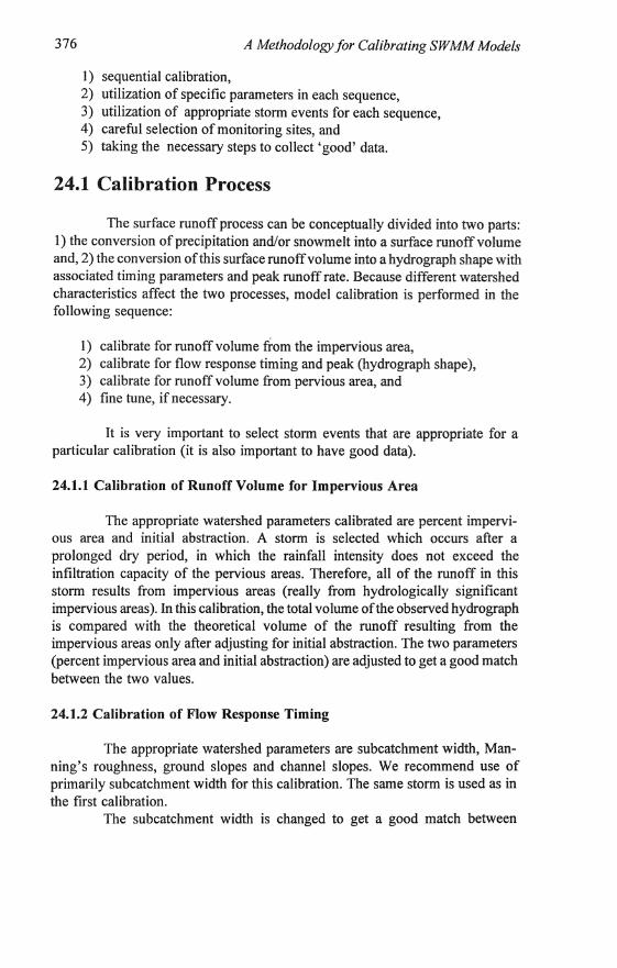
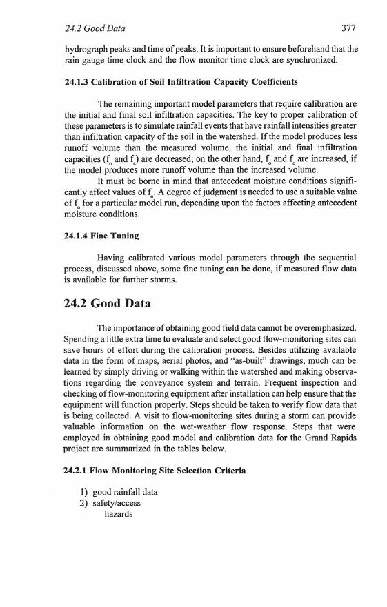
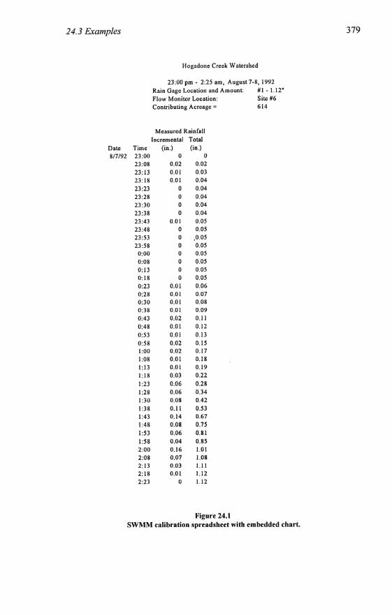
Upon the completion of a SWMM input file, a tedious, yet worthwhile, value-by-value comparison of the input data was made against system data shown on the model schematic and the project notes. Microsoft EXCEL spreadsheets with an embedded chart, provide an organized means of archiving the calibration data, rainfall data, and SWMM simulation results. Figure 24.1 is a sample spreadsheet. At the top of the spreadsheet, the title block identifies the watershed, the calibration data monitoring site, the date and time of the rain event, and the total rainfall amount. The second section in the spreadsheet is rainfall (total rainfall and incremental rainfall for the entire rain event). The third section summarizes the calibration adjustments made to the original SWMM

24.3 Examples 379

Hogadone Creek Watershed

23:00 pm - 2:25 am, August 7-8,1992 Rain Gage Location and Amount: #1 - 1.12" Flow Monitor Location: Site #6 Contributing Acreage = 614

Measured Rainfall

Incrementa' Total

Date Time (in.) (in.) 817192 23:00 0 0

23:08 0.02 0.02

23:13 O.O! 0.03 23:18 0.01 0.04

23:23 0 0.04 23:28 0 0.04 23:30 0 0.04

23:38 0 0.04

23:43 0.01 0.05 23:48 0 0.05 23:53 0 ,0.05 23:58 0 0.05

0:00 0 0.05 0:08 0 0.05 0:13 0 0.05 0:18 0 0.05

0:23 0.01 0.06 0:28 0.01 0.07 0:30 0.01 0.08 0:38 0.01 0.09 0:43 0.02 O.ll

0:48 0.01 0.12

0:53 0.01 0.13 0:58 0.01 0.15 1:00 0.D2 0.17 I:OB O.ol 0.18

1:13 Ooll! 0.19 !:IS 0.03 0.22

1:23 0.06 0.28 1:28 0.06 0.34 1:30 0.08 0.42 1:38 0.1\ 0.53 1:43 0.14 0.67 1:48 0.08 0.75 1:53 0.06 0.81

1:58 0.04 O.gS 2:00 0.16 1.01 2:08 0.07 /.08 2:13 0.03 !.II 2:18 0.01 1.12 2:23 0 1.12

Figure 24.1 SWMM calibration spreadsheet with embedded chart.

380

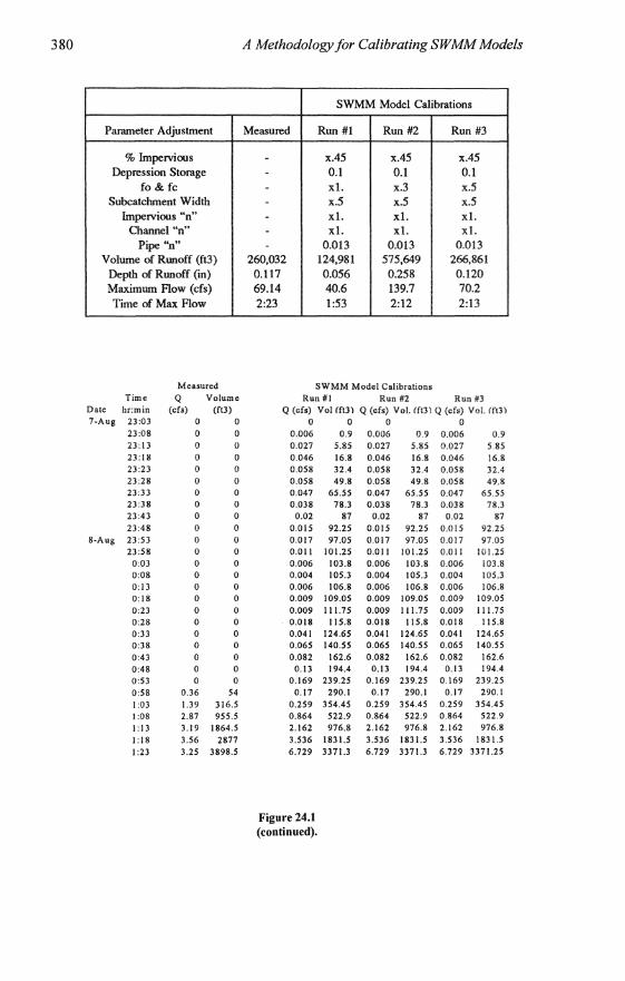
Parameter Adjustment

% Impervious Depression Storage

focftfc Subcatchment Width

Impervious "n" Oiannel "n"

Pipe "n" Volume of Runoff (ft3)

Depth of Runoff (m) Maximum Flow (cfs) Time of Max Flow

Measured Time Q Volume

Dale hr:min (crs) (ft3) 7·Aug 23:03 0 0

23:08 0 0 23:13 0 0 23:18 0 0 23:23 0 0 23:28 0 0 23:33 0 0 23:38 0 0 23:43 0 0 23:48 0 0

8-Aug 23:53 0 0 23:58 0 0 0:03 0 0 O:OS 0 0 0:13 0 0 0:18 0 0 0:23 0 0 0:28 0 0 0:33 0 0 0:38 0 0 0:43 0 0 0:48 0 0 0:53 0 0 0:S8 0.36 54 1:03 1.39 316.S 1:08 2.87 9SS.S 1:13 3.19 1864.S 1:18 3.56 2877 1:23 3.25 389S.S

A Methodology for Calibrating SWMM Models

SWMM Model Calibrations

Measured Run #1 Run #2 Run ##3

- x.45 x.45 x.45 - 0.1 0.1 0.1 - xl. x.3 x.s - x.s x.s x.s - xl. xl. xl. - xl. xl. xl. - 0.013 0.013 0.013

260,032 124,981 575,649 266,861 0.117 0.056 0.258 0.120 69.14 40.6 139.7 70.2 2:23 1:53 2:12 2:13

SWMM Model Calibration. Run'l Run til Run'3

Q (crs) Vol (ft3) Q (crs) Vol. (fill Q (crs) Vol. (ft))

0 0.006 0.027 0.046 0.058 0.058 0.047 0.038

0.02 0.015 0.017 0.011 0.006 0.004 0.006 0.009 0.009

. 0.018 0.041 0.065 0.082

0.13 0.169

0.17 0.2S9 0.864 2.162 3.536 6.729

Figure 24.1 (continued).

0 0 0.9 0.006

5.85 0.027 16.8 0.046 32.4 0.058 49.8 0.058

6S.S5 0.047 78.3 0.D38

87 0.02 92.25 0.015 97.05 0.017

101.25 0.011 103.8 0.006 105.3 0.004 106.8 0.006

109.05 0.009 11I.7S 0.009

115.8 0.018 124.65 0.041 140.55 0.065

162.6 0.082 194.4 0.\3

239.25 0.169 290.1 0.17

354.45 0.259 522.9 0.864 976.8 2.162

1831.S 3.536 3371.3 6.729

0 0.9 0.006 0.9

5.85 0.027 S.8S 16.8 0.046 16.8 32.4 0.058 32.4 49.8 0.OS8 49.8

65.SS 0.047 65.55 78.3 0.038 78.3

87 0.02 87 92.25 om5 92.25 97.05 0.017 97.05

101.25 0.011 101.25 103.8 0.006 103.8 105.3 0.004 105.3 106.8 0.006 106.8

109.0S 0.009 109.0S 111.75 0.009 111.75

115.8 0.018 115.8 124.65 0.041 124.65 140.55 0.06S 140.55

162.6 0.082 162.6 194.4 0.13 194.4

239.25 0.169 239.2S 290.1 0.17 290.1

354.4S 0.259 354.45 522.9 0.864 S22.9 976.8 2.162 976.8

1831.S 3.536 1831.5 3371.3 6.729 3371.25

24.3 E:>:amp/es 381

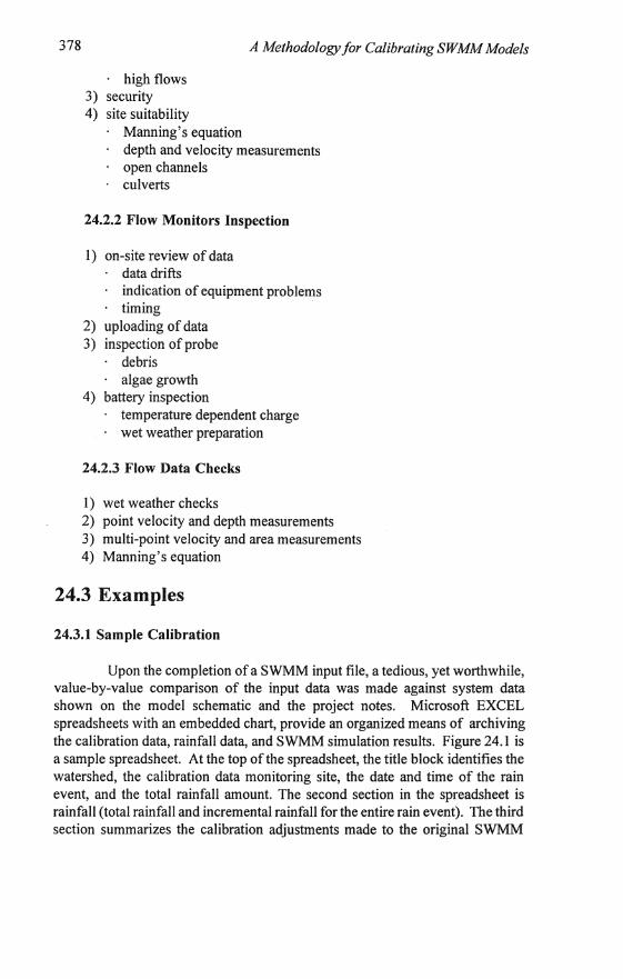
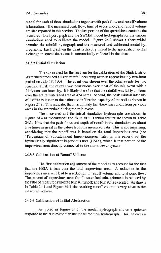
model for each of three simulations together with peak flow and runoff volume information. The measured peak flow, time of occurrence, and runoff volume are also reported in this section. The last portion ofthe spreadsheet contains the measured flow hydrograph and the SWMM model hydrographs for the various simulations used to calibrate the model. Figure 24.2 shows a chait which contains the rainfall hyetograph and the measured and calibrated model hy­drographs. Each graph on the chart is directly linked to the spreadsheet so that a change in spreadsheet data is automatically reflected in the chart.

24.3.2 Initial Simulation

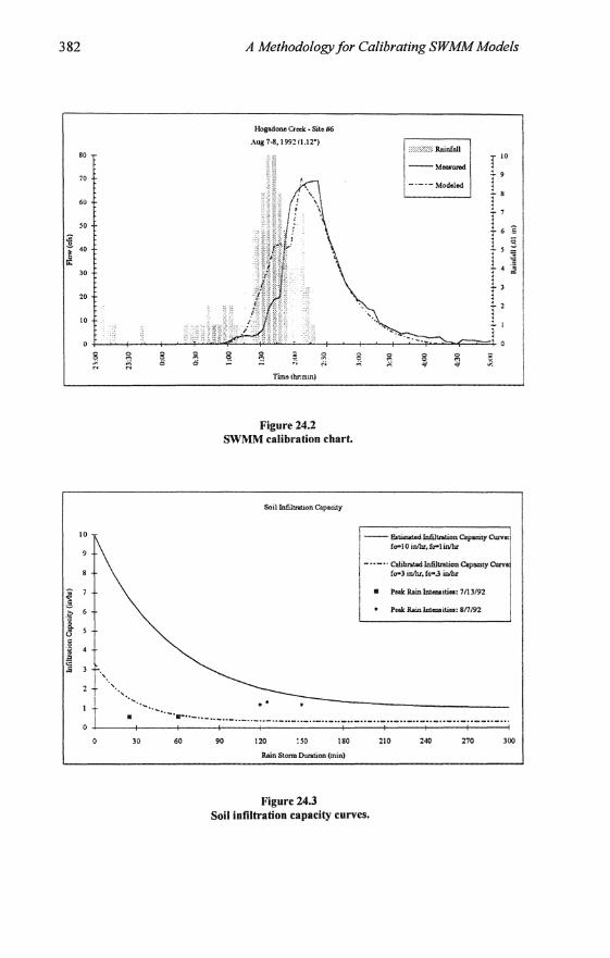
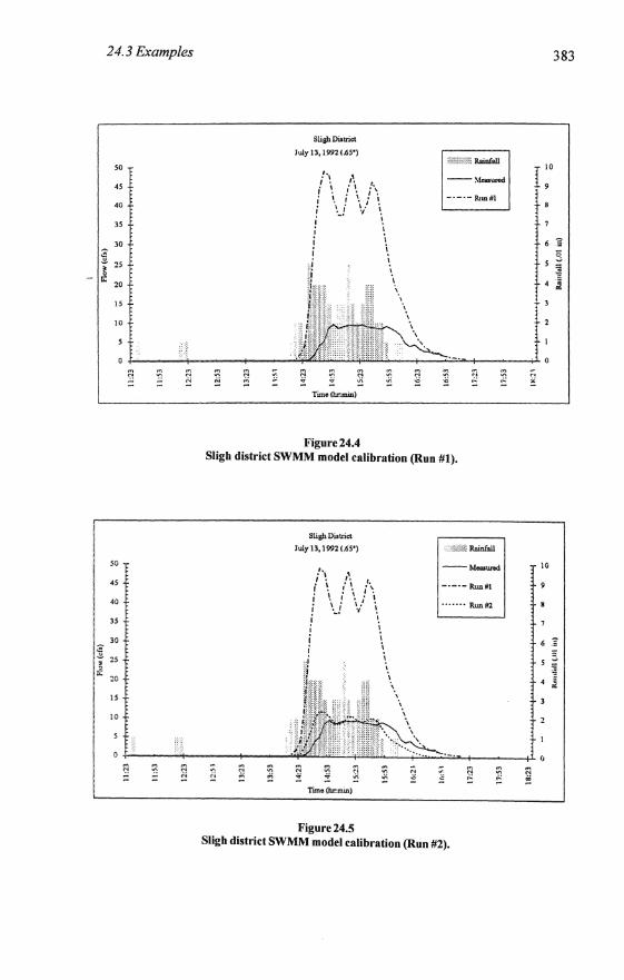
The storm used for the first run for the calibration of the Sligh District Watershed produced a 0.65" rainfall occurring over an approximately two-hour period on July 13, 1993. The event was chosen over the other events for two reasons. First, the rainfall was continuous over most of the rain event with a fairly constant intensity. It is likely therefore that the rainfall was fairly uniform over the entire watershed area of 424 acres. Second, the peak rainfall intensity of O.6"lhr is less than the estimated infiltration capacity of the soil as shown in Figure 24.3. This indicates that it is unlikely that there was runoff from pervious areas in the watershed during the rain event.

The measured and the initial simulation hydrographs are shown in Figure 24.4 as "Measured" and "Run #1." Tabular results are shown in Table 24.1. Note that the peak flows and depth of runoff in the simulation are about five times as great as the values from the measured data. This is not surprising, considering that the runoff area is based on the total impervious area (see "Percentage of Subcatchment Imperviousness" later in this paper), not the hydraulically significant impervious area (HSIA), which is that portion of the impervious area directly connected to the storm sewer system.

24.3.3 Calibration of Runoff Volume

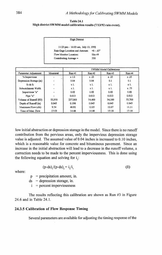
The first calibration adjustment of the model is to account for the fact that the HSIA is less than the total impervious area. A reduction in the impervious area will lead to a reduction in runoff volume and total peak flow. The percent of impervious areas for all watershed subcatchments is reduced by the ratio of measured runoffto Run # I runoff; and Run #2 is executed. As shown in Table 24.1 and Figure 24.5, the resulting runoff volume is very close to the measured volume.

24.3.4 Calibration of Initial Abstraction

As noted in Figure 24.5, the model hydrograph shows a quicker response to the rain event than the measured flow hydrograph. This indicates a

382

80

70

60

so

i 00

~ 30

20

10

10

-'-.

A Methodology for Calibrating SWMM Models

HopeI .... en •. Site 116

Aug 7-8. 1992 II .12')

Figure 14.2 SWMM calibration chart.

Soilloli\lnwm.Cq>ociily

g'M$I'liRaiDl'Aill

--Moaound

- ._.- MedoIecI

--EstiamdlaliJbMiaoaCapocity ( ... 10_ .... 1_

- •• - •• CaIihroIod laliJbMiaoa eapa=y r .. 3illillr .... .3_

' .. '~' .. , .. , .. , ..... -.. -.. -.. -.. -.. -~.~ .. -.. -.. -.-.. -.. -.. -.. -.. -"-"-"-"-"-"-"--"-'" 30 60 120 :so 180 210 240 270 300

Figure 24.3 Soil infiltration capacity curves.

24.3 Examples

so

45

40

35

30

i 25

~ 20

10

so

45

40

35

IS

10

... ~ ~ '" ~

~

... g ~

B

S1ishDillri<>t

July 13,19921.65')

f~~ I~ i ~ " I. {\

i '. i \ i ' ',' ~_f \; ,

i 1 i i i i \

~ ... g '" :

T .... Ou:min)

Figure 24.4

\ \ \

... '" =

--~

-·---R.nn.l

~ ~ ..

~ .. :!! ;.:

Sligh district SWMM model calibratiou (Run #1).

~ ~ '" t!

SlishDillri<>t July 13,1992 (.65')

" • , r.

, ; \ i\ ~\' \' . .... 1 'I' \

~ :;: ... .. :! :!

T_Ihr.min)

Figure24.S

i i i \ \

i

... '" ~

"-., .. i ..

Ea;;;ilWllillaiDfaU ----'-'-Ruaill

.. ..... Rualll

~ ! g ~

Sligh districtSWMM model calibration (Run #2).

383

10

9

6 :s

0 .. ,.

10

0

~

384 A Methodology for Calibrating SWMM Models

Table 24.1 Sligh district SWMM model calibration results (7/13/92 rain event).

Sligh District

11:23 pm - 16:03 am, July 13, 1992 Rain Gage Location and Amoum: =6 - .6S·

Flow Monitor Location: Site fI9

Couiributing A<nage - 330

SWMM Model Calibnlioas

Parameter Adjusiment Measured Run .. 1 Run1J2 Run .. 3 Run 114 % Impervious - x 1.0 - x.23 x.25 x.2S

Depression Storage (in) - 0.04 0.04 0.1 0.1

fo8tfc - xl. x I. xl. xl. SubcatchmelJl Width - xl. xl. xl. x.7S

Impervious -n° - 0.02 0.02 0.02 0.02

Pipe "n" - 0.013 0.013 0.013 0.013

Volwne of Runolf (ftJ) S3,9~ 237,000 54,-100 54,100 53,700 Depth of Runolf (in) 0.045 0.198 0.045 O.04S 0.045

~mumFlow(cf.) 9.54 48.92 12.0S 12.07 lUI

Time of Max. Flow 15:03 14:48 14:48 15:18 15:18

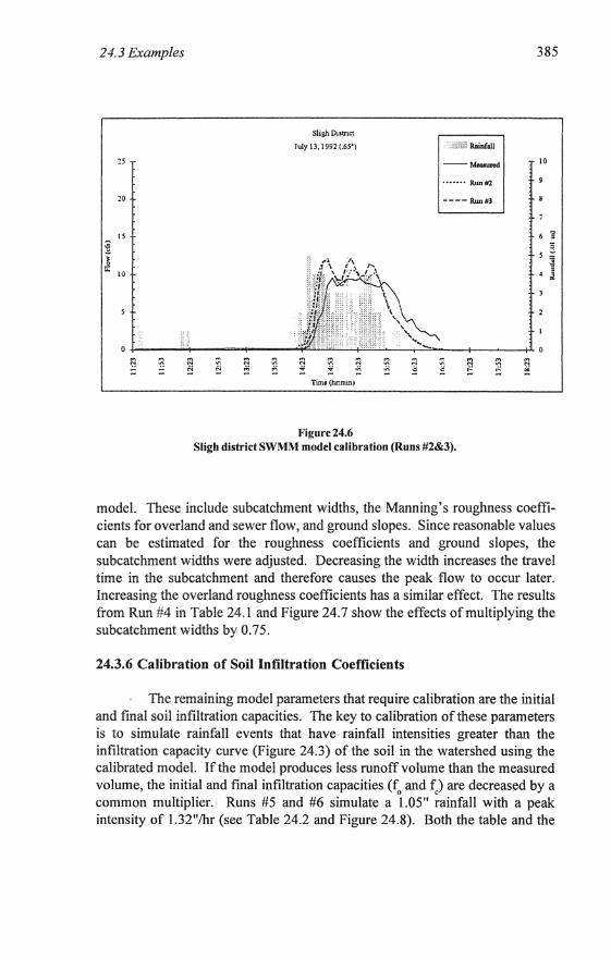
low initial abstraction or depression storage in the model. Since there is no runoff contribution from the pervious areas, only the impervious depression storage value is adjusted. The assumed value of 0.04 inches is increased to 0.10 inches, which is a reasonable value for concrete and bituminous pavement. Since an increase in the initial abstraction will lead to a decrease in the runoff volume, a correction needs to be made to the percent imperviousness. This is done using the following equation and solving for i2:

where: p = precipitation amount, in.

ds = depression storage, in. = percent imperviousness

(1)

The results reflecting this calibration are shown as Run #3 in Figure 24.6 and in Table 24.1.

24.3.5 Calibration of Flow Response Timing

Several parameters are available for adjusting the timing response of the

24.3 Examples

2S

20

IS

~ Ii: 10

0

g ~ ~ ~

.., 3 ::! ~

~ .;;

SlithDutnct

July 13.1992 (.65')

::l ::! .... N

! :! Vi

r .... (hr. .... '

Figure 24.6

- .... -·······111111112

---- Runf13

... .., ~ ::l ~ ~ N ~

Vi ~ :!! ~

Sligb district SWMM model calibration (Runs #2&3).

385

10

9

~

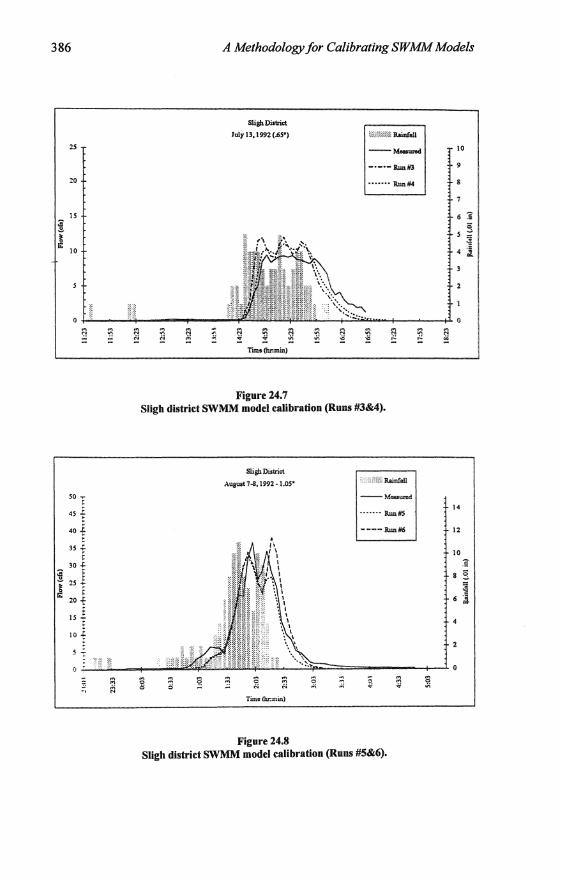
model. These include subcatchment widths, the Manning's roughness coeffi­cients for overland and sewer flow, and ground slopes. Since reasonable values can be estimated for the roughness coefficients and ground slopes, the subcatchment widths were adjusted. Decreasing the width increases the travel time in the subcatchment and therefore causes the peak flow to occur later. Increasing the overland roughness coefficients has a similar effect. The results from Run #4 in Table 24.1 and Figure 24.7 show the effects of multiplying the subcatchment widths by 0.75.

24.3.6 Calibration of Soil Infiltration Coefficients

The remaining model parameters that require calibration are the initial and tmal soil infiltration capacities. The key to calibration of these parameters is to simulate rainfall events that have rainfall intensities greater than the infiltration capacity curve (Figure 24.3) of the soil in the watershed using the calibrated model. If the model produces less runoff volume than the measured volume, the initial and final infiltration capacities (fo and fc) are decreased by a common multiplier. Runs #5 and #6 simulate a 1.05" rainfall with a peak intensity of 1.32"/hr (see Table 24.2 and Figure 24.8). Both the table and the

386

25

:0

15 .. .!'-

~ fi:

10

0

§ ~ ::l t!

A Methodology for Calibrating SWMM Models

-. 3 ~

f.! ~

Sligh Di.trict

luIy 13.1992(.65')

~ ~

~ ~ '_(hr.""")

Figure 24.7

S'@}?';-;'_oll

--Meoau...:l

-'---lImN3

, •••••.• lim'" ,

~ ~ ~ ::l ~ N

~ g v; :! ~

Sligh district SWMM model calibration (RUDS #3&4).

a ~ 9. ~

a a

SlighDatri<t

Auguot 1-8,1992. 1.0S·

~ ::l ~ N N

Timclhr.min)

Figure 24.8

< ,';'; ltullfoll I -!~I ••.•••• lImll5 !

----1Wn1i6

0 ::l .0:; "' 'i v

Sligh district SWMM model calibration (Runs #5&6).

~

~

12

10

.5

24.3 Examples

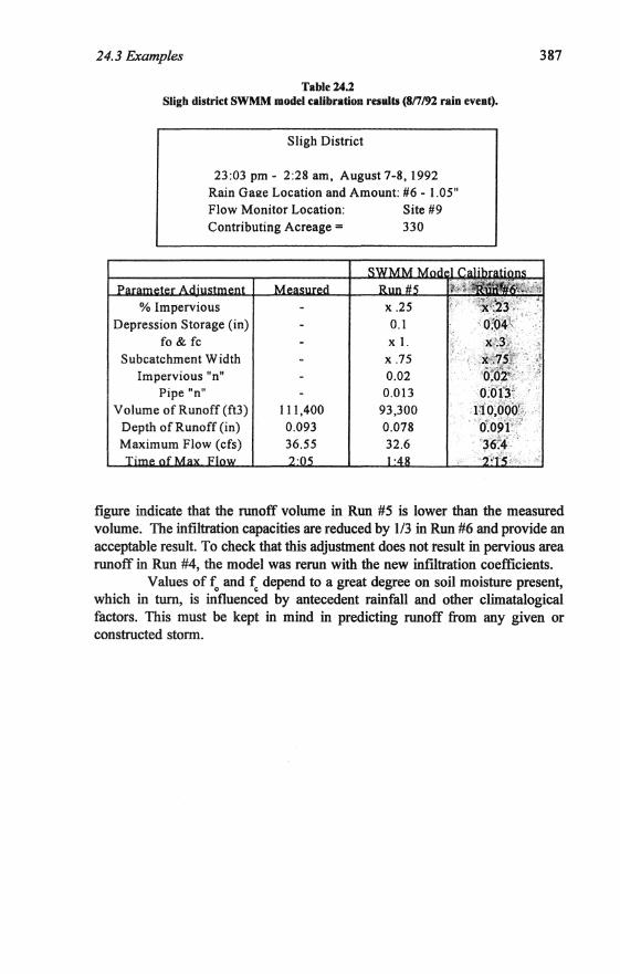
Table 24.2 Sligh district SWMM model calibration results (Sn 192 rain event).

Sligh District

23:03 pm - 2:28 am, August 7-8,1992 Rain Gage Location and Amount: #6 - l.OS" Flow Monitor Location: Site #9 Contributing Acreage = 330

% Impervious Depression Storage (in)

fo & fc Subcatehment Width

Impervious "n" Pipe "n"

Volume of Runoff (ft3) Depth of Runoff (in) Maximum Flow (efs)

111.400 0.093

xl. x.75 0.02

0.013 93,300 0.078

387

figure indicate that the runoff volume in Run #5 is lower than the measured volume. The infiltration capacities are reduced by 1/3 in Run #6 and provide an acceptable result. To check that this adjustment does not result in pervious area runoff in Run #4, the model was rerun with the new inftltration coefficients.

Valnes of t;, and ft depend to a great degree on soil moisture present, which in tum, is influenced by antecedent rainfall and other climatalogical factors. This must be kept in mind in predicting runoff from any given or constructed storm.