A method to include directional spreading of waves into

November 2003

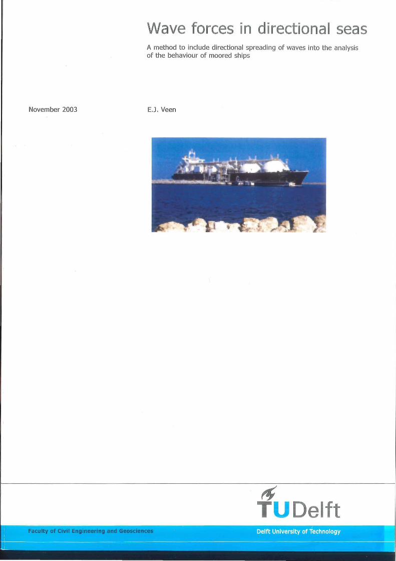
Wave forces in directional seas A method to include directional spreading of waves into the analysis of the behaviour of moored ships

E.J. Veen

~ T U Delft

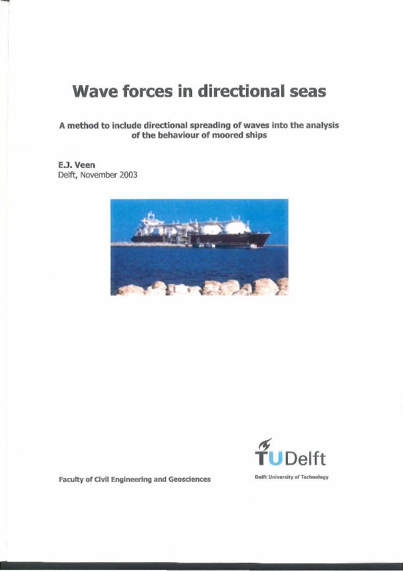
Wave forces in directional seas

A method to include directional spreading of waves into the analysis of t he behaviour of moored ships

E.J. Veen Delft, November 2003

tf T Delft

Faculty of Civil Engineering and Geosciences Delft University of Technology

~ TUDelft Wave forces in directional seas


A method to include directional spread ing of waves into the analysis of the behaviour of moored ships

Author: ir. E.J.Veen TU Delft

Delft, November 2003

'A method to include directiona l spread ing of waves into the analysis of the behaviour of moored ships' Page 1

~ TUDelft

Abstract


When studying the behaviour of moored sh ips under the influence of environmental conditions time domain simulation programmes can be very useful. Termsim 11 1 is a time domain simulation program to analyze the dynamic behaviour of a moored tanker subject to wind, waves and current. The mooring system can be a single point mooring, a multi buoy mooring or a jetty terminal. The program predicts the mooring loads and tanker motions when the system is exposed to operational environmental conditions. However, Termsim 11 is not capable of taking directional spreading of waves into account.

Since in practice the waves do not tend to come from one specific direction it seems wise to include this directional spreading effect into the calculations. To make this possible for calculations made with Termsim 11, a separate -Matlab based- program has been developed , that generates time series of wave forces in which the designer can specify the wave spectrum as a function of frequency and direction .

This program, developed with Matlab, consists of several parts. First of all the desired spectrum has to be specified. Secondly the hydrodynamic file has to be read by Matlab in order to store the first order and second order transfer functions. Now the wave forces can be calculated. Matlab starts with the first order wave forces and subsequently calculates the force due to the set down (bound long wave force) and the second order drift force. Finally all three forces are superimposed.

To visualise the results for the designer all forces are saved as a figure Upeg format) in a user-specified directory. The time series of wave forces are stored as text files in the same directory.

1 MARIN , Termsim 11, Wageningen , 1998

'A method to include directional spread ing of waves into the analysis of the behaviour of moored ships' Page 2

T

~ TUDelft

Index


Abstract .................................................................. ........................ ......... ................................. 2

List of figures ........................................................................................................................... 3

1 Introduction ....................................................................................................................... 4 2 Problem analysis .............................................................................................................. 5

2.1 Problem defin ition ........... .. ......... ........ .. .. .. ...... ........ ........ ............................ .... .. ............ 5 2.2 Research objective ... .. ........................... ... .... ......... .................. ... .. .... ..... ................... ... 5

3 Theoretical background ................................................................................................... 6 3.1 lntroduction .. .. ... ... ..... ... ..... ........ ... ..... .. ... ..... .. ............ ....................... ..... .... ..... ..... ....... .. 6 3.2 Directional spreading ...... ... .. .. ... ...... ... ..... .. .. .... ............... ...... ....... ................................. 6

3.2.1 The Jonswap spectrum ... ...... .... .. ...... ..... .. ............................. .. .. .. ......................... 7 3.2.2 The Pierson-Moskowitz spectrum .......... ... ............. ........ ....... .......................... ..... 8 3.2.3 The Gaussian spectrum ....... .. ......... ... ......... ... .............................. ............... .. .. ... .. 9

3.3 Transfer functions (RAO's) .. ... .................................. ..... .. .......................................... 10 3.4 First order wave forces ........... ...... ... ........... ................................ ..... .......................... 10 3.5 Second order wave drift forces ...... ................................... .. .. .................................... 12 3.6 Wave set down .. ...... ......... .... .... ...... .... ................. ... .... ..... ... ......... ..... ...... ......... .... ... ... 14 3.7 Total wave force .. .......... .. .......................................................................................... 16

4 Users manual for the matlab wave force computation scripts .................................. 17 4.1 lntroduction ............. ..... .. .. ...... ... .................... ..... ......................... .. .. .... .... ........... .. ...... 17 4.2 How to change the input parameters .... ......... .. ....... ....... .. ..... ..... .. ............................. 18 4.3 Hydrodynamic files .............. .. ... ..... .. ... ............. .. ...... ........ .. .. .... .. ....... .................. ....... 19

Appendix 1: Structure of the saved parameters by matlab

List of figures

Figure 3-1: Jonswap wave energy spectrum ........ ................ .. .... .. .. ........................................... 7 Figure 3-2: Piersson-Moskowitz wave energy spectrum ...... .. .. ............................................. .. .. 8 Figure 3-3: Gaussian wave energy spectrum ...... .... .............................. ... .... ............................. 9 Figure 3-4: Time series of first order wave forces ........ .......... ... ............ .. ................. .. ...... ....... 11 Figure 3-5: Time series of second order wave drift forces .... ......................... ...... ................. . 13 Figure 3-6: First order waves and the correspond ing wave set-down .................. .......... ......... 15 Figure 3-7: Wave forces due to wave set-down .. ... .. .................... .. .. ....................................... 15 Figure 3-8: Time series of total wave forces ........ .. .......................... ........................................ 16


~ TUDelft

1 Introduction


A method of including the effect of directional spreading of waves into the analysis of the behaviour of moored ships using the time domain simulation program Termsim 11 has been developed which has resulted in a matlab-based software tool.

This report gives the problem analysis in chapter 2 after which in chapter 3 the theoretical background of this study is treated. Finally chapter 4 gives a users manual for the developed software tool.

'A method to include directional spreading of waves into the analysis of the behaviour of moored ships' Page 4

-

~ TUDelft

2 Problem analysis

2.1 Problem definition


Termsim 11, a time domain simulation programmes for the analysis of the behaviour of moored LNG carriers is not capable of taking directional spread ing of waves into account.

2.2 Research objective

The development of a computer program that produces input files with time series of wave forces for the computation of motions in which the directional spread ing of waves is taken into account. The hydrodynamic properties of the vessel, such as the transfer functions for wave forces, are available from the resu lts of a frequency domain diffraction model.

'A method to include directiona l spread ing of waves into the analysis of the behaviour of moored sh ips' Page 5


3 Theoretical background

3.1 Introduction

When a vessel is berthed it may be under the influence of either sea or swell waves. lt is possible to take a different direction for the sea and swell spectrum. However, it is not possible to include directional spreading within the same spectrum. The sea or swell are considered to be long-crested waves. For a better consideration of wave forces, directional spread ing of the wave spectrum shou ld be taken into account when studying the behaviour of moored ships.

3.2 Directional spreading

When considering directional spreading, a wave spectrum can be formulated in terms of direction and frequency. Two options are available for that purpose.

Option 1: S(oo) and 8(8), with the directional spread ing independent of the wave frequency.

A formulation, which is often used in practice, is the "cosine-squared rule" .

S(w ,B) = S(w) ·A · COS111 (B-B)

In which : ~IT

A = scaling parameter: A- 1 = f cos111 B dB -~11"

m = spread ing parameter e = mean wave direction

Option 2: S(oo,8), with the directional spreading dependent of the wave frequency.

The first option is sufficiently accurate and widely used in practice and will therefore be used for this project.

'A method to incl ude directional spreading of waves into the analysis of the behaviour of moored ships' Page 6

(3.1)


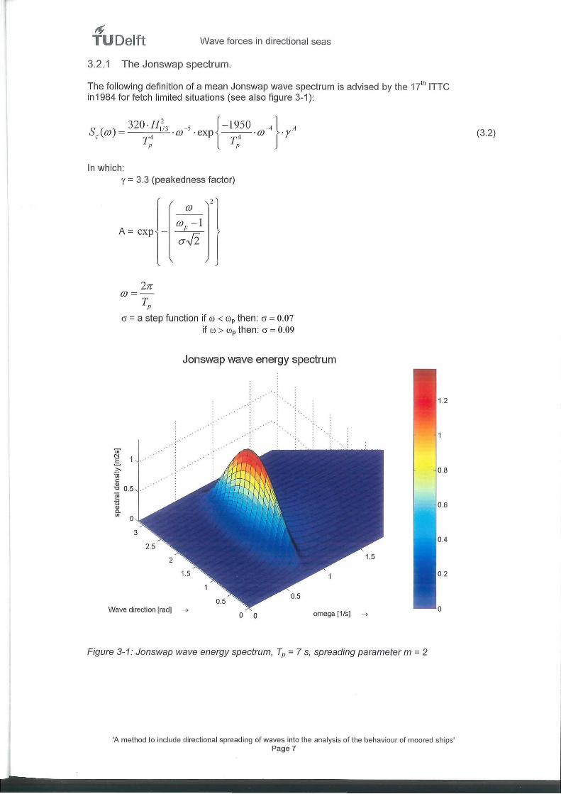
3.2.1 The Jonswap spectrum.

The following definition of a mean Jonswap wave spectrum is advised by the 17'h ITTC in1984 for fetch limited situations (see also f igure 3-1 ):

S ( ) 320·H,~3 -5 {-1950 -4} A OJ = . OJ . exp . OJ . r ' T4 T4

p p

In which: y = 3.3 (peakedness factor)

OJ

OJP-} A = exp - CJ.fi

27r OJ=-

~)

2

cr = a step function if w < wp then: cr = 0.07 if w > wp then : cr = 0.09

Jonswap wave energy spectrum

7ii' ~ 1 ..

£;"iii c:: Q)

-o 0.5 ~ u Q) 0. If) 0

Wave direction [rad] ~ 0 0 omega [1/s] ~

Figure 3-1: Jonswap wave energy spectrum, Tp = 7 s, spreading parameter m = 2

0. 8

0.6


(3.2)

tf TUDelft Wave forces in directional seas

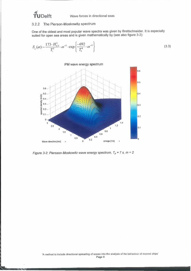
3.2.2 The Pierson-Moskowitz spectrum

One of the oldest and most popular wave spectra was given by Brettschneider. it is especially suited for open sea areas and is given mathematically by (see also figure 3-2):

S ( ) 173 · H1~3 _5 {-692 _4 } OJ = ·OJ ·exp --·OJ

' T4 T4 I I

PM wave energy spectrum

0.5

0.6 ,

_ O.S v· 0.4 "' N

.s 0.4 z. ·v; c 0.3 , . ., 0.3 '0

~ 0.2 ,. 0 ., Q_

"' 0.1 .2

0

Wave direction [rad] ---> 0 omega [1/s] --->

Figure 3-2: Piersson-Moskowitz wave energy spectrum, Tp = 7 s, m = 2

'A method to include directional spreading of waves into the analysis of the behaviour of moored sh ips' Page 8

(3.3)


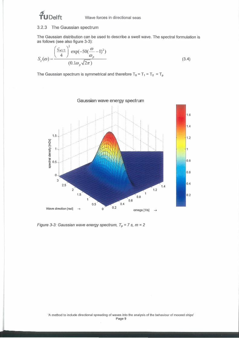
3.2.3 The Gaussian spectrum

The Gaussian distribution can be used to describe a swel l wave. The spectral formulation is as fol lows (see also figure 3-3):

( ''~13 )' exp( -50(: -I)') S, (w) = r (3.4)

(O.Iwp.fi;)

The Gaussian spectrum is symmetrical and therefore T0 = T1 = T2 = Tp

(jj' N

E. z. ·u; c <!) '0

1.5

1'! t> 0.5 <!) c. (/)

0

Gaussian wave energy spectrum

··: ..

Wave direction [rad] --? 0 omega [1/s] --?

Figure 3-3: Gaussian wave energy spectrum, Tp = 7 s, m = 2

1.2

0.8


~ TUDelft

Transfer functions (RAO 's)


The coupling between wave height and wave period on the one hand and the wave force on the other hand is determined by the transfer functions (Response Amplitude Operators, RAO's). These parameters are available in the so-called hydrodynamic files, which contain the hydrodynamic properties of a vessel for a specific waterdepth. We can distinguish first order and second order transfer functions.

3.3 First order wave forces

After splitting up the wave energy spectrum into a series of cosines we have a mathematical equation that gives us a time series of wave elevations as a function of wave frequency (m) and wave direction (8).

11 111

r (t) = "" r . COS((JJ . t + & .) ~-~ ~~ ~IJ I J IJ i=] J=l

The hydrodynamic file provides us with the RAO's for the 1st order wave height and the 1st

order wave force: FCil

c;( l )

~(I) =I" Ill/ F ( t ) - c; . k • cos (J) + & . + lp . k I,J, i.j 1,) 1,) ,

W=i !J=j c; i ,j ,k

k=l,2 .. ,6

F = RAO for (J) and k-mode

c; i,j ,k i. J

c;i,k = Wave amplitude

(J) = Frequency i.j

t = Time

&i,j = Random phase angle

(/Ji ,j,k = Phase angle for wave exciting forces (with (1)1

and k-mode)

The first order RAO's are taken from the hydrodynamic file . When no RAO is available for a specific combination of wave frequency and direction, a linear interpolation will be made between the four closest points (two for the frequency and two for the direction) .

If the wave frequency is higher than the highest frequency from the hydrodynamic file, no interpolation is possible. In that case the value of the RAO from the highest frequency will be used .

By now multiplying each element of the wave height time series with the corresponding RAO and superimposing them we obtain the total first order wave force.

For the surge, sway and heave motion we get time series of wave forces (kN). For the pitch, roll and yaw motion we get time series of wave moments (kNm). Figure 3-4 gives an example of the matlab output of such a first order wave signal.

'A method to include directiona l spreading of waves into the analysis of the behaviour of moored sh ips' Page 10

-

(3.5)

(3.6)

If TUDelft Wave forces in directional seas

First order wave forces X 104

t t 2 z z

~ ~ <1J 0 E ~ ~ -2 3: (f)

0 600 1200 1800 2400 3000 3600 0 600 1200 1800 2400 3000 3600 X 10

4 Time [s] ~ X 105 Time[s] ~

t t

z 5 E'

~ z <1J 0 ~ 0

~ <1J E

<1J ~ -1 ~ -5 .c

u <1J 8: -2 I

0 600 1200 1800 2400 3000 3600 0 600 1200 1800 2400 3000 3600 X 106 Time[s] ~ X 106 Time [s] ~

t 2 t

E' 1 E' 0.5 z z ~ 0 ~ 0 <1J <1J

E -1 u

~ ~ -0.5

'5 -2 '5 -1 0:: 0::

0 600 1200 1800 2400 3000 3600 0 600 1200 1800 2400 3000 3600 Time[s] ~ Time [s] ~

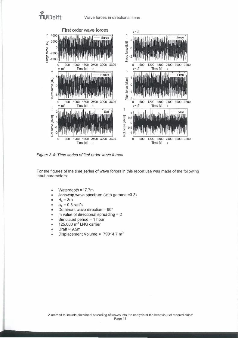
Figure 3-4: Time series of first order wave forces

For the figures of the time series of wave forces in this report use was made of the following input parameters:

• • • • • • • • • •

Waterdepth =17.7m Jonswap wave spectrum (with gamma =3.3) Hs = 3m mp = 0.8 rad/s Dominant wave direction = 90° m value of directional spreading = 2 Simulated period = 1 hour 125.000 m3 LNG carrier Draft= 9.5m Displacement Volume= 79014.7 m3

'A method to include directiona l spreading of waves into the analysis of the behaviour of moored sh ips' Page 11


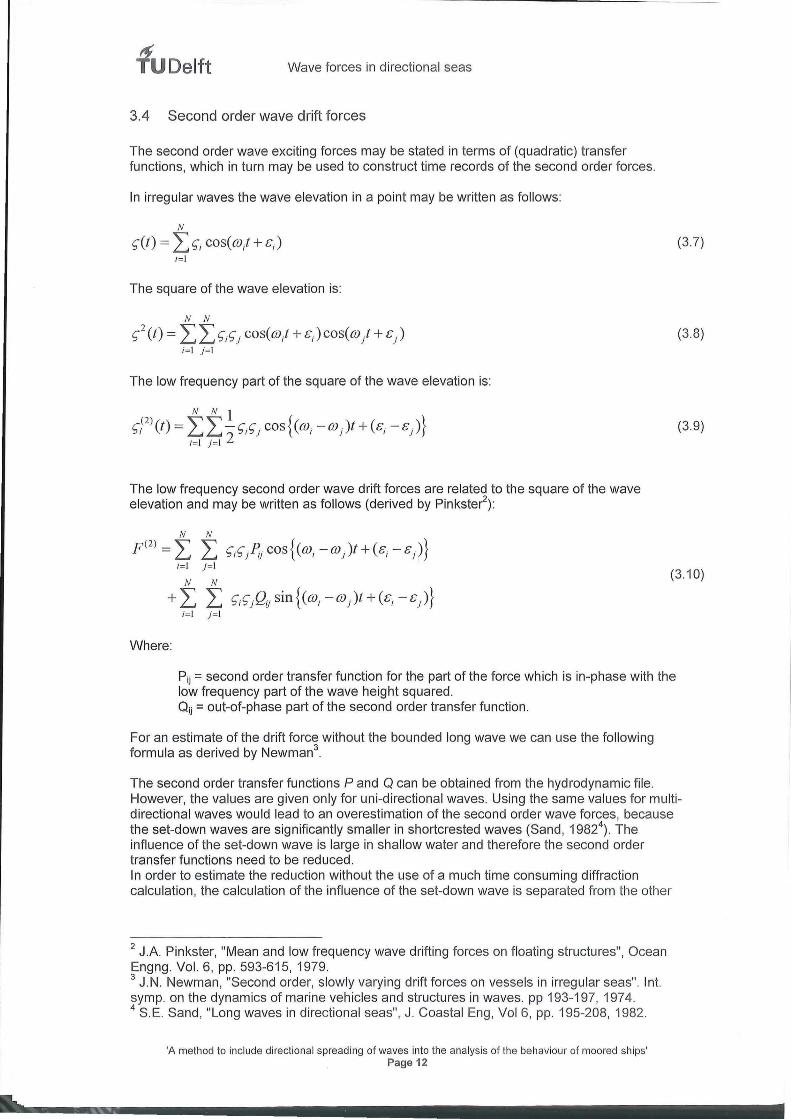
3.4 Second order wave drift forces

The second order wave exciting forces may be stated in terms of (quadratic) transfer functions, which in turn may be used to construct time records of the second order forces .

In irregular waves the wave elevation in a point may be written as follows:

N

~(t) = I ~i cos(mJ+tJ i=i

The square of the wave elevation is:

N N

~2 (t) = I I ~i~J cos( mJ + &i) cos( m l + &1 )

i=i J= i

The low frequency part of the square of the wave elevation is:

The low frequency second order wave drift forces are related to the square of the wave elevation and may be written as follows (derived by Pinkste~) :

N N

F (2) =I I ~i~/~1 cos{ (mi -m;)t + (&i- &;)}

(3.7)

(3.8)

(3.9)

i=i J= i

N N (3 .1 0)

+I I ~i~JQ!i sin { (mi -m;)t + (&i -&;)}

Where:

i=i J=i

P1i = second order transfer function for the part of the force which is in-phase with the low frequency part of the wave height squared. Q1i = out-of-phase part of the second order transfer function.

For an estimate of the drift force without the bounded long wave we can use the following formula as derived by Newman3

.

The second order transfer functions P and Q can be obtained from the hydrodynamic file. However, the values are given only for uni-directional waves. Using the same values for multidirectional waves would lead to an overestimation of the second order wave forces, because the set-down waves are significantly smaller in shortcrested waves (Sand, 1982\ The influence of the set-down wave is large in shallow water and therefore the second order transfer functions need to be reduced . In order to estimate the reduction without the use of a much time consuming diffraction calculation, the calculation of the influence of the set-down wave is separated from the other

2 J.A. Pinkster, "Mean and low frequency wave drifting forces on floating structures", Ocean Engng. Vol. 6, pp. 593-615, 1979. 3 J. N. Newman, "Second order, slowly varying drift forces on vessels in irregular seas" . lnt. symp. on the dynamics of marine vehicles and structures in waves. pp 193-197, 1974. 4 S.E. Sand, "Long waves in directional seas", J. Coastal Eng, Vol 6, pp. 195-208, 1982.


tf TUDelft Wave forces in directional seas

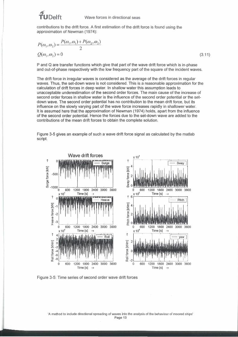
contributions to the drift force. A first estimation of the drift force is found using the approximation of Newman (1974):

(3.11)

P and Q are transfer functions which give that part of the wave drift force which is in-phase and out-of-phase respectively with the low frequency part of the square of the incident waves.

The drift force in irregular waves is considered as the average of the drift forces in regular waves. Thus, the set-down wave is not considered. This is a reasonable approximation for the calculation of drift forces in deep water. In shallow water this assumption leads to unacceptable underestimation of the second order forces. The main cause of the increase of second order forces in shallow water is the influence of the second order potential or the setdown wave. The second order potential has no contribution to the mean drift force, but its influence on the slowly varying part of the wave force increases rapidly in sha llower water. lt is assumed here that the approximation of Newman (1974) holds, apart from the influence of the second order potential. Hence the forces due to the set-down wave are added to the contributions of the mean drift forces to obtain the complete solution.

Figure 3-5 gives an example of such a wave drift force signal as calculated by the matlab script.

t

z ~ -1

Wave drift forces

1200 1800 2400 3000 3600 Time[s] ~

0 600 1200 1800 2400 3000 3600 x 10' Time [s] ~

t 4~~~~~~u=~~~

600 1200 1800 2400 3000 3600 Time [s] ~

t ~4 z ~ <!)

~ 2 .E ~ ~o~~~~~~~~~rr=~

0 600 1200 1800 2400 3000 3600 x 105 Time [s] ~

t 6 r-~--~~--~~c=~~

E4 z ~ <!)

~ 2 .E .r::. 0 a: 0 """'-.E!.!lw:.!L..!.!!.

t

'E 2 z ~

~ 0 .E '5

0 600 1200 1800 2400 3000 3600 x 10' Time [s] ~

~ -2 L_~_L~--~~~--~~

0 600 1200 1800 2400 3000 3600 Time[s] ~

Figure 3-5: Time series of second order wave drift forces

'A method to include directional spreading of waves into the ana lysis of the behaviour of moored ships' Page 13

~ TUDelft

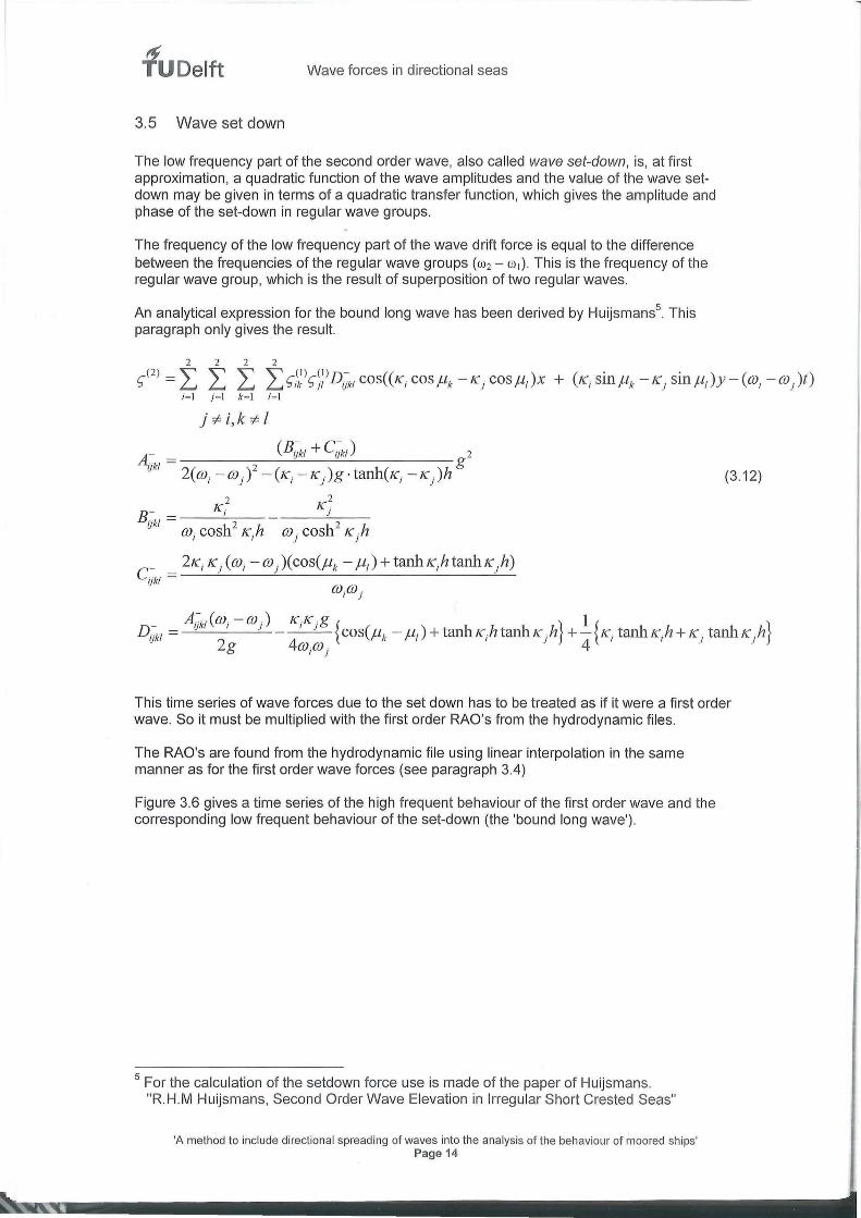
3.5 Wave set down


The low frequency part of the second order wave, also called wave set-down, is, at first approximation, a quadratic function of the wave amplitudes and the value of the wave setdown may be given in terms of a quadratic transfer function, which gives the amplitude and phase of the set-down in regular wave groups.

The frequency of the low frequency part of the wave drift force is equal to the difference between the frequencies of the regular wave groups (ro2 - ro 1). This is the frequency of the regular wave group, which is the result of superposition of two regular waves.

An analytical expression for the bound long wave has been derived by Huijsmanss This paragraph only gives the result.

2 2 2 2

C2l -" " " " Cll CllD- (( ) ( . . ) ( )t) ; - L... L... L... L... ;;k ;JI ijkt cos K; cos Jik - K i cos Ji1 x + K; sm Jik - KJ sm p1 y- OJ; - OJJ . i= J j=J k= l 1=1

(3.12)

2

B- K; "kl-I) OJ cosh 2

K h I I

_ 2K; K j ( OJ; - OJ j )( COS(Jik - j.11) + tanh K;h tanh K jh) cijkl = --""------"-------------"--

OJ;OJ j

This time series of wave forces due to the set down has to be treated as if it were a first order wave. So it must be multiplied with the first order RAO's from the hydrodynamic files.

The RAO's are found from the hydrodynamic file using linear interpolation in the same manner as for the first order wave forces (see paragraph 3.4)

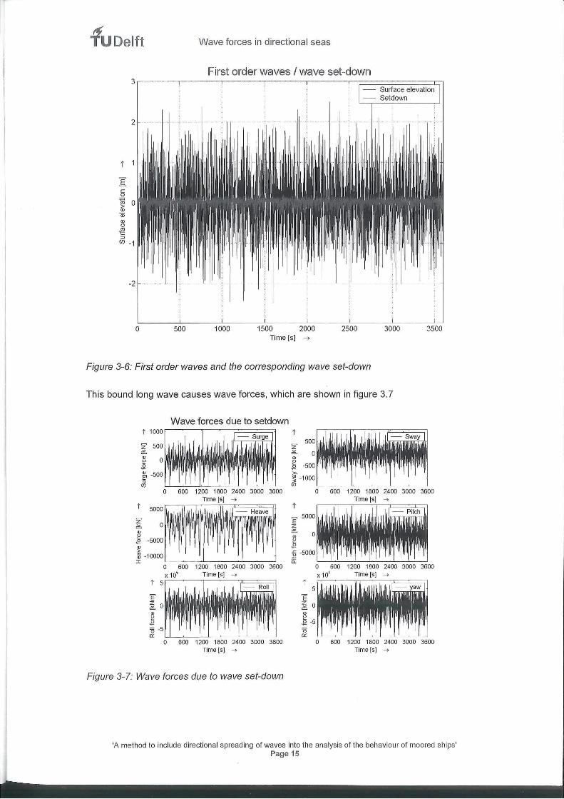
Figure 3.6 gives a time series of the high frequent behaviour of the first order wave and the corresponding low frequent behaviour of the set-down (the 'bound long wave').

5 For the calculation of the setdown force use is made of the paper of Hu ijsmans. "R.H.M Huijsmans, Second Order Wave Elevation in Irregular Short Crested Seas"

'A method to include directiona l spread ing of waves into the analysis of the behaviour of moored ships' Page 14

~ TUDelft

t

I c 0

~ Qj Q) u

~ ::J (f) -1

0 500


First order waves I wave set-down

1000 1500 2000 2500 Time[s] ~

Figure 3-6: First order waves and the corresponding wave set-down

3000

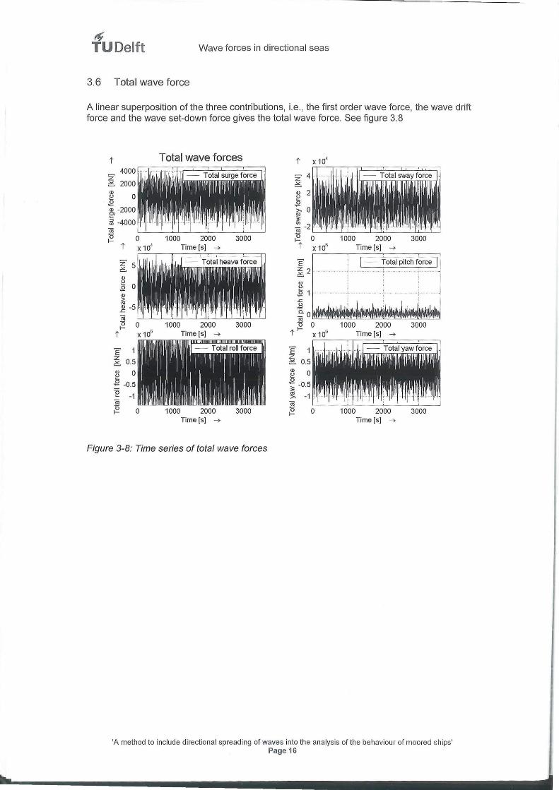
This bound long wave causes wave forces, which are shown in figure 3.7

z 500 =. ~ 0 .g ~ -500

Wave forces due to setdown i

500 z =. 0

" " ~ -500 ,., ~ -1000

3500

::J (J) (J) L_~ __ _h __ ~ __ _L __ ~--~

0 600 1200 1800 2400 3000 3600 --> Time Is) -->

t 5000 t

z E' 5000

=. 0 z

" =. 0 ~ " .g -5000 ~ " > :§ -5000 lll -10000 I 0::

0 600 1200 1800 2400 3000 3600 0 600 1200 1800 2400 3000 3600 X 10

5 Time Is) --> X 104

-->

t 5 t 5

E' E' z 0

z 0 =. =. " " ~ ~ -5 '5 -5 0 0:: 0::

0 600 1200 1800 2400 3000 3600 Time Is) --> -->

Figure 3-7: Wave forces due to wave set-down


tf TU Delft Wave forces in directional seas

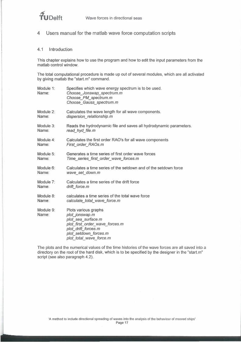
3.6 Total wave force

A linear superposition of the three contributions, i.e., the first order wave force, the wave drift force and the wave set-down force gives the total wave force. See figure 3.8

t Total wave forces

z ~ 2000 <1J u 0 .8

<1J -2000 ~ ~ -4000 (ii

~ 0 1000 2000 t x 10' Time [s] ~

z 5 ~ <1J ~ Q 0

~ "' ~ -5 (ii

~ 0 1000 2000 t x 106 Time (s] ~

3000

3000

E' B. 0.5

<1J 0 ~ Q -0.5

=e -1

[1111 1 11~~/l 'll ,r l/ I '111j' I :i;:;·i;: ;;;;;:!

j ,llt~.~L~Ii.lllhll!lil~l~ll] ii~JJIJi ll .IJ ~~~Ill 0 1000 2000 3000

Time[s] ~

Figure 3-8: Time series of total wave forces

t X 104

z 4 ~ <1J 2 ~ Q >- 0 "' ~ -2 "' ~t 0 1000

X 106

2000 3000 Time[s] ~

E' I - Total pitch force I g2 ················· ....

E' z ~ 0.5

~ 0 .8 5 ~ -0.

~ -1

0

. . . . . . . . . . . . . . . . . . . . . . . . . .

1000 2000 3000 Time[s] ~

'A method to include directiona l spreading of waves into the analysis of the behaviour of moored ships' Page 16

h~------------------........... ~

I I I


4 Users manual for the matlab wave force computation scripts

4 .1 Introduction

This chapter explains how to use the program and how to ed it the input parameters from the matlab control window.

The total computational procedure is made up out of several modules, which are all activated by giving matlab the "start.m" command.

Module 1: Name:

Module 2: Name:

Module 3: Name:

Module 4: Name:

Module 5: Name:

Module 6: Name:

Module 7: Name:

Module 8: Name:

Module 9: Name:

Specifies which wave energy spectrum is to be used. Choose_ Jonswap _spectrum. m Choose_PM_spectrum.m Choose_ Gauss_spectrum.m

Calculates the wave length for all wave components. dispersion _relationship. m

Reads the hydrodynamic file and saves all hydrodynamic parameters. read_hyd_file.m

Calculates the first order RAO's for all wave components First_ order_RA Os, m

Generates a time series of first order wave forces Time_series_first_order_wave_forces.m

Calculates a time series of the setdown and of the setdown force wave_ set_ down. m

Calculates a time series of the drift force drift_ force. m

calculates a time series of the total wave force calculate_total_wave_force.m

Plots various graphs plot_jonswap.m plot_ sea_ surface. m plot_ first_ order_ wave_ forces. m plot_ drift_ forces. m plot_ setdown_ forces. m plot_total_wave_force.m

The plots and the numerical values of the time histories of the wave forces are all saved into a directory on the root of the hard disk, which is to be specified by the designer in the "start. m" script (see also paragraph 4.2).



4 .2 How to change the input parameters

The input parameters that can be edited are listed in the main matlab script: 'start.m'. After opening this file with the matlab ed itor, one can ed it the fo llowing features:

• The waterdepth, Since the calculation is performed for a certa in waterdepth th is must be defined in the main script. Be sure that the used waterdepth is the same as the one for which the hydrodynamic file was developed!

• The total calculation time (defined as "timespan")

• The significant wave height: (defined as "H_sig")

• The peak frequency of the wave spectrum: (defined as "omega_p")

• The dominant wave direction: (defined as "dom_wave_d ir")

• The desired wave energy spectrum This is defined in module 1. The three options are:

• "Choose_Jonswap_spectrum.m" • "Choose_PM_spectrum.m" • "Choose_Gauss_spectrum.m"

• The desired number of frequency and directional intervals into which the spectrum is split up. Be aware that the system might get unstable when one chooses this number to high. Eight intervals (default value) is a recommended value.

• The " y value" for the Jonswap spectrum.

• The "m value" for the directional spreading.

• The folder on your hard drive in which the plots and text files with time series are saved.

• The name of the hydrodynamic file.



4.3 Hydrodynamic files

The hydrodynamic files contain the hydrodynamic properties of a specific vessel in a certain water depth . Coefficients such as the added mass and the damping parameters are all listed in the files.

Each time simulation program (Termsim, BAS, SHIP-MOORINGS, etc) specifies this file in a different manner. The consequence of this is that for each different "hydrodynamic file format" a different matlab module has to be written to read the files and to use the data for the subsequent calculations.

This research program has used the Termsim format. This paragraph explains how to save the file in order for matlab to be able to read the data. Appendix I gives more information on how the parameters in the hydrodynamic file are stored by matlab.

Saving the hydrodynamic file for use by matlab

• Open the hydrodynamic file in MS Excel. • When opening the file, excel will ask you how to separate the variables.

• Choose the option " Fixed width" • Subsequently insert the so-called "breaklines" on those places where the variables

have to be separated. • At this point the hydrodynamic file has been converted into an excel file . • Save using "save as csv file" . This causes the text file to be saved with commas as

separation sign in between the columns. • Now open the file with a text editor and make sure that all the variables are separated

with only one comma. • Now scroll to the part of the file where the 2nd order RAO's are given and look at the part

that gives the OMEGA2 parameters. • At the end of the last line of the OMEGA2 record there could be one or more

commas. • If so, delete them. • If not, the file is ready to be used.

• Save the file as a text file


tf TUDelft

Literature


[1] R.H.M. Huijsmans, "Second Order Wave Elevation in Irregular Short Crested Seas", technical report, MARIN, 2002

[2] J.M.J. Journee and W.W. Massie, "Offshore Hydromechanics", Lecture notes, Delft University of Technology, January 2001

[3] J.N. Newman, "Second order, slowly varying drift forces on vessels in irregular seas". lnt. symp. on the dynamics of marine vehicles and structures in waves. pp 193-197, 1974.

[4] J.A. Pinkster, "Mean and low frequency wave drifting forces on floating structures", Ocean Engng. Vol. 6, pp. 593-615, 1979.

[5] S.E. Sand, "Long waves in directional seas", J. Coastal Eng, Vol 6, pp. 195-208, 1982


Appendix 1: Structure of the saved parameters by matlab

This appendix describes which parameters are saved by matlab and which names they are given in the matlab workspace.

Part 1: General information on the hyd. file.

1. The IDENT data is omitted.

2. The following REFS data is stored:

• REFS.keyword REFS

• REFS.waterdepth Waterdepth

• REFS.vesseldraft Draft of the ship

• REFS.Z_coordinate z coordinate of the waterline

3. The following SPRING data is stored :

• SPRING.keyword SPRING

• SPRING.vessel_displacement In m3

• SPRING.water line area In m2 - -

• SPRING.centre_of_flotation X coordinate van 'centre of floatation'

• SPRING.centre_of_buoyancy X coordinate of the centre of buoyancy

• SPRING.transverse_metacentric_height Transversal metacentre height, measured from the keel (KMT)

• SPRING.Iongitudinal_metacentric_height Longitudinal metacentre height, measured from the keel (KML)

4. The following PARA data is stored:

• PARA.keyword PARA

• PARA.number_of_frequencies The number of frequencies for which 1st order RAO's have been developed.

• PARA.number of wave directions The number of wave directions for which 1st order RAO's have been

developed. • PARA.number_of_symmetry_planes

The number of symmetry planes

Part 2:added mass and damping coefficients

-------- -- ---- ---- -------- -- -------- ----Since these parameters are not used for the calculation of the wave forces they are NOT included in the 'read_hyd_ file" script. However, they ARE included in the 'read_hyd_file2" script.

-------------------- - ----- ------ --------

• ADMASS(i ,ii,degree of freedom) • Added mass coefficients • i and ii have values between 1 t/m 6. • Degree of freedom has a value between 1 t/m 6. • 1 =surge

2 =sway 3 = heave 4 = roll 5 = pitch 6 = yaw

• BDAMP(i,jj,degree of freedom) • Damping coefficients • i and ii have values between 1 t/m 6. • Degree of freedom has a value between 1 t/m 6.

1 =surge 2 = sway 3 = heave 4 = roll 5 =pitch 6 = yaw

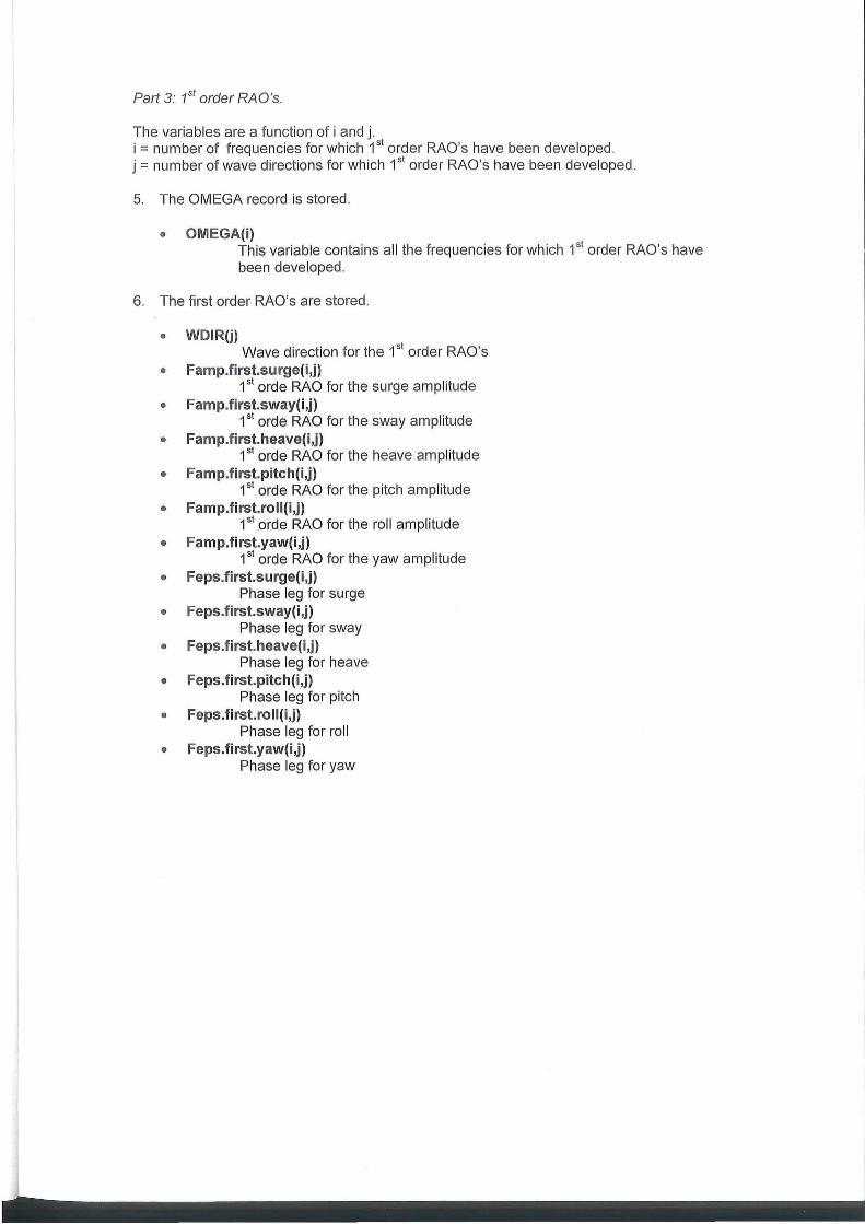
Part 3: 1st order RAO's.

The variables are a function of i and j. i = number of frequencies for which 1st order RAO's have been developed. j = number of wave directions for which 1st order RAO's have been developed.

5. The OMEGA record is stored.

6.

• OMEGA(i) This variable contains all the frequencies for which 1st order RAO's have been developed.

The first order RAO's are stored.

• WDIR(j) Wave direction for the 1st order RAO's

• Famp.first.surge(i,j) 1st orde RAO for the surge amplitude

• Famp.first.sway(i,j) 1st orde RAO for the sway amplitude

• Famp.first.heave(i,j) 1st orde RAO for the heave amplitude

• Famp.first.pitch(i,j) 1st orde RAO for the pitch amplitude

• F amp. first. roll(i,j) 1st orde RAO for the roll amplitude

• Famp.first.yaw(i,j) 1st orde RAO for the yaw amplitude

• Feps.first.surge(i,j) Phase leg for surge

• Feps.first.sway(i,j) Phase leg for sway

• Feps.first.heave(i,j) Phase leg for heave

• Feps.first.pitch(i,j) Phase leg for pitch

• Feps.first.roll(i,j) Phase leg for roll

• Feps.first.yaw(i,j) Phase leg for yaw

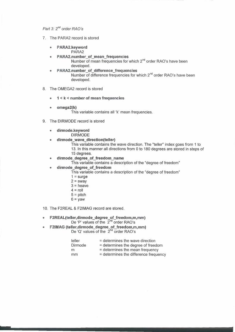
Part 3: 2nd order RAO's

7. The PARA2 record is stored

• PARA2.keyword PARA2

• PARA2.number_of_mean_frequencies Number of mean frequencies for which 2nd order RAO's have been developed.

• PARA2.number_of_difference_frequencies Number of difference frequencies for which 2nd order RAO's have been developed.

8. The OMEGA2 record is stored

• 1 < k < number of mean frequencies

• omega2(k) This variable contains all 'k' mean frequencies.

9. The DIRMODE record is stored

• dirmode.keyword DIRMODE

• dirmode_wave_direction(teller) This variable contains the wave direction. The "teller" index goes from 1 to 13. In this manner all directions from 0 to 180 degrees are stored in steps of 15 degrees.

• dirmode_degree_of_freedom_name This variable contains a description of the "degree of freedom"

• dirmode_degree_of_freedom This variable contains a description of the "degree of freedom" 1 =surge 2 =sway 3 =heave 4 =roll 5 =pitch 6 = yaw

10. The F2REAL & F21MAG record are stored .

• F2REAL(teller,dirmode_degree_of_freedom,m,mm) De 'P' values of the 2nd order RAO's

• F21MAG (teller,dirmode_degree_of_freedom,m,mm) De 'Q' values of the 2nd order RAO's

teller Dirmode m mm

= determines the wave direction = determines the degree of freedom = determines the mean frequency = determines the difference frequency

Documents

A method to include directional spreading of waves into