H O S T E D B Y The Japanese Geotechnical Society

Soils and Foundations

Soils and Foundations 2016;56(1):33–43

http://d0038-0

E-mPeer

x.doi.org/806/& 201

ail addrereview un

ncedirect.comw.elsevier.com/locate/sandf

www.sciejournal homepage: ww

A method to compute the non-linear behaviour of piles underhorizontal loading

Gianpiero Russo

Department of Civil, Architectural and Environmental Engineering (D.I.C.E.A), Federico II University, Via Claudio 21, Naples, Italy

Received 24 September 2014; received in revised form 28 July 2015; accepted 16 September 2015Available online 20 February 2016

Abstract

The empirical evidence for vertical piles under horizontal or lateral loading is firstly reviewed. The load–deflection relationship is nonlinearfrom the early stages of loading, while the load–moment relationship is nearly linear. Moving from the available experimental evidence, typicaldesign issues are addressed and a validation of the widespread Broms’ method is then carried out. To predict the pile–soil interaction, a computercode, NAPHOL, based on a hybrid BEM approach, is fully presented and discussed. A limiting pressure profile, coupled with a cut-off procedure,allows the method to cope with the nonlinear behaviour. Simple guidelines and equations, to calibrate the model parameters, are derived on thebasis of the back-analysis of a significant number of case histories. The program is finally used to throw light on the mechanism of the pile–soilinteraction under horizontal loading.& 2016 The Japanese Geotechnical Society. Production and hosting by Elsevier B.V. All rights reserved.

Keywords: Analysis; Computer code; Horizontal load; Piles; BEM

1. Introduction

The behaviour of piles under horizontal loading is different fromthat under vertical loading. When axially loaded, the structuralsection of the piles does not have a large influence on the pile–soilinteraction, as the compression stress is generally very low com-pared to the strength of the pile material (wood, steel or concrete).With an increasing load, failure may occur, if at all, at the interfacebetween the pile and the soil where the limiting values of theavailable shaft friction are attained. Under horizontal loading, onthe contrary, the piles are primarily subjected to bending momentand shear, and their structural section has a large influence on thepile response both at the serviceability limit state (SLS) and at theultimate limit state (ULS).

10.1016/j.sandf.2016.01.0036 The Japanese Geotechnical Society. Production and hosting by

ss: pierusso@unina.itder responsibility of The Japanese Geotechnical Society.

Furthermore, the behaviour of a vertical axially loaded piledepends essentially on the properties of the soil immediatelyadjacent to the shaft and below the base, which are the zoneslargely affected by the pile installation process. Accordingly, thebehaviour of a vertically loaded pile, particularly its bearingcapacity, is markedly affected by the installation process and thetechnology adopted (Poulos et al., 2001; Mandolini et al., 2005).Under horizontal loading, the pile–soil interaction is confined to avolume of soil which has a different shape and location (Ng et al.,2001; Rollins et al., 2005). Such a volume is typically confined tothe upper part of the pile shaft, close to the ground surface, andit develops at a larger distance from the pile shaft. For this rea-son, a major part of this volume of soil is not affected by thepile installation. However, the available full-scale experimentalevidence on piles tested under horizontal loading is less exhaustivethan for vertical loading. Furthermore, most of the availablehorizontal loading tests have been conducted on piles whoseheads were free to rotate even though pile heads in actual

Elsevier B.V. All rights reserved.

050

100150200250300350400

0,000 0,020 0,040 0,060 0,080

Load

(kN

)

displacement (m)

Vibration PileTsubasa Pile

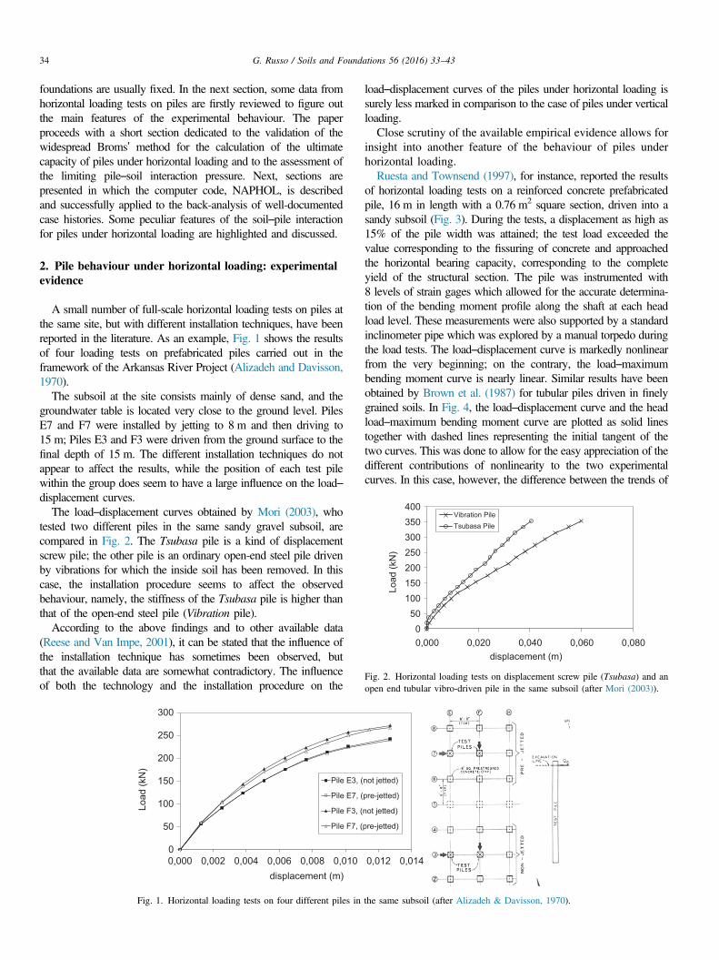
Fig. 2. Horizontal loading tests on displacement screw pile (Tsubasa) and anopen end tubular vibro-driven pile in the same subsoil (after Mori (2003)).

G. Russo / Soils and Foundations 56 (2016) 33–4334

foundations are usually fixed. In the next section, some data fromhorizontal loading tests on piles are firstly reviewed to figure outthe main features of the experimental behaviour. The paperproceeds with a short section dedicated to the validation of thewidespread Broms’ method for the calculation of the ultimatecapacity of piles under horizontal loading and to the assessment ofthe limiting pile–soil interaction pressure. Next, sections arepresented in which the computer code, NAPHOL, is describedand successfully applied to the back-analysis of well-documentedcase histories. Some peculiar features of the soil–pile interactionfor piles under horizontal loading are highlighted and discussed.

2. Pile behaviour under horizontal loading: experimentalevidence

A small number of full-scale horizontal loading tests on piles atthe same site, but with different installation techniques, have beenreported in the literature. As an example, Fig. 1 shows the resultsof four loading tests on prefabricated piles carried out in theframework of the Arkansas River Project (Alizadeh and Davisson,1970).

The subsoil at the site consists mainly of dense sand, and thegroundwater table is located very close to the ground level. PilesE7 and F7 were installed by jetting to 8 m and then driving to15 m; Piles E3 and F3 were driven from the ground surface to thefinal depth of 15 m. The different installation techniques do notappear to affect the results, while the position of each test pilewithin the group does seem to have a large influence on the load–displacement curves.

The load–displacement curves obtained by Mori (2003), whotested two different piles in the same sandy gravel subsoil, arecompared in Fig. 2. The Tsubasa pile is a kind of displacementscrew pile; the other pile is an ordinary open-end steel pile drivenby vibrations for which the inside soil has been removed. In thiscase, the installation procedure seems to affect the observedbehaviour, namely, the stiffness of the Tsubasa pile is higher thanthat of the open-end steel pile (Vibration pile).

According to the above findings and to other available data(Reese and Van Impe, 2001), it can be stated that the influence ofthe installation technique has sometimes been observed, butthat the available data are somewhat contradictory. The influenceof both the technology and the installation procedure on the

0

50

100

150

200

250

300

0,000 0,002 0,004 0,006 0,008 0,010

Load

(kN

)

displacement (m)

Pile E3, (

Pile E7, (

Pile F3, (

Pile F7, (

Fig. 1. Horizontal loading tests on four different piles in

load–displacement curves of the piles under horizontal loading issurely less marked in comparison to the case of piles under verticalloading.Close scrutiny of the available empirical evidence allows for

insight into another feature of the behaviour of piles underhorizontal loading.Ruesta and Townsend (1997), for instance, reported the results

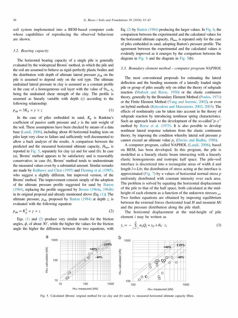
of horizontal loading tests on a reinforced concrete prefabricatedpile, 16 m in length with a 0.76 m2 square section, driven into asandy subsoil (Fig. 3). During the tests, a displacement as high as15% of the pile width was attained; the test load exceeded thevalue corresponding to the fissuring of concrete and approachedthe horizontal bearing capacity, corresponding to the completeyield of the structural section. The pile was instrumented with8 levels of strain gages which allowed for the accurate determina-tion of the bending moment profile along the shaft at each headload level. These measurements were also supported by a standardinclinometer pipe which was explored by a manual torpedo duringthe load tests. The load–displacement curve is markedly nonlinearfrom the very beginning; on the contrary, the load–maximumbending moment curve is nearly linear. Similar results have beenobtained by Brown et al. (1987) for tubular piles driven in finelygrained soils. In Fig. 4, the load–displacement curve and the headload–maximum bending moment curve are plotted as solid linestogether with dashed lines representing the initial tangent of thetwo curves. This was done to allow for the easy appreciation of thedifferent contributions of nonlinearity to the two experimentalcurves. In this case, however, the difference between the trends of

0,012 0,014

not jetted)

pre-jetted)

not jetted)

pre-jetted)

the same subsoil (after Alizadeh & Davisson, 1970).

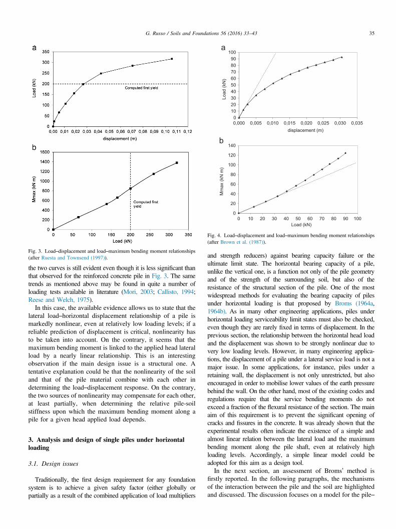
Fig. 3. Load–displacement and load–maximum bending moment relationships(after Ruesta and Townsend (1997)).

0102030405060708090

100

0,000 0,005 0,010 0,015 0,020 0,025 0,030 0,035

Load

(kN

)

displacement (m)

0

20

40

60

80

100

120

140

0 10 20 30 40 50 60 70 80 90 100M

max

(kN

m)

Load (kN)

Fig. 4. Load–displacement and load–maximum bending moment relationships(after Brown et al. (1987)).

G. Russo / Soils and Foundations 56 (2016) 33–43 35

the two curves is still evident even though it is less significant thanthat observed for the reinforced concrete pile in Fig. 3. The sametrends as mentioned above may be found in quite a number ofloading tests available in literature (Mori, 2003; Callisto, 1994;Reese and Welch, 1975).

In this case, the available evidence allows us to state that thelateral load–horizontal displacement relationship of a pile ismarkedly nonlinear, even at relatively low loading levels; if areliable prediction of displacement is critical, nonlinearity hasto be taken into account. On the contrary, it seems that themaximum bending moment is linked to the applied head lateralload by a nearly linear relationship. This is an interestingobservation if the main design issue is a structural one. Atentative explanation could be that the nonlinearity of the soiland that of the pile material combine with each other indetermining the load–displacement response. On the contrary,the two sources of nonlinearity may compensate for each other,at least partially, when determining the relative pile-soilstiffness upon which the maximum bending moment along apile for a given head applied load depends.

3. Analysis and design of single piles under horizontalloading

3.1. Design issues

Traditionally, the first design requirement for any foundationsystem is to achieve a given safety factor (either globally orpartially as a result of the combined application of load multipliers

and strength reducers) against bearing capacity failure or theultimate limit state. The horizontal bearing capacity of a pile,unlike the vertical one, is a function not only of the pile geometryand of the strength of the surrounding soil, but also of theresistance of the structural section of the pile. One of the mostwidespread methods for evaluating the bearing capacity of pilesunder horizontal loading is that proposed by Broms (1964a,1964b). As in many other engineering applications, piles underhorizontal loading serviceability limit states must also be checked,even though they are rarely fixed in terms of displacement. In theprevious section, the relationship between the horizontal head loadand the displacement was shown to be strongly nonlinear due tovery low loading levels. However, in many engineering applica-tions, the displacement of a pile under a lateral service load is not amajor issue. In some applications, for instance, piles under aretaining wall, the displacement is not only unrestricted, but alsoencouraged in order to mobilise lower values of the earth pressurebehind the wall. On the other hand, most of the existing codes andregulations require that the service bending moments do notexceed a fraction of the flexural resistance of the section. The mainaim of this requirement is to prevent the significant opening ofcracks and fissures in the concrete. It was already shown that theexperimental results often indicate the existence of a simple andalmost linear relation between the lateral load and the maximumbending moment along the pile shaft, even at relatively highloading levels. Accordingly, a simple linear model could beadopted for this aim as a design tool.In the next section, an assessment of Broms’ method is

firstly reported. In the following paragraphs, the mechanismsof the interaction between the pile and the soil are highlightedand discussed. The discussion focuses on a model for the pile–

G. Russo / Soils and Foundations 56 (2016) 33–4336

soil system implemented into a BEM-based computer codewhose capabilities of reproducing the observed behaviourare shown.

3.2. Bearing capacity

The horizontal bearing capacity of a single pile is generallyevaluated by the widespread Broms’ method, in which the pile andthe soil are assumed to behave as rigid–perfectly plastic bodies andthe distribution with depth of ultimate lateral pressure pult on thepile is assumed to depend only on the soil type. The ultimateundrained lateral pressure in clay is assumed as a constant profilein the case of a homogeneous soil layer with the value of 9su, subeing the undrained shear strength of the clay. The profile isassumed as linearly variable with depth (z) according to thefollowing relationship:

pult ¼ 3Kp � γ � z ð1ÞIn the case of piles embedded in sand, Kp is Rankine’s

coefficient of passive earth pressure and γ is the unit weight ofthe soil. These assumptions have been checked by means of a database (Landi, 2006), including about 40 horizontal loading tests onpiles kept very close to failure and sufficiently well documented toallow a back analysis of the results. A comparison between thepredicted and the measured horizontal ultimate capacity, Hlim, isreported in Fig. 5, separately for clay (a) and for sand (b). In case(a), Broms’ method appears to be satisfactory and is reasonablyconservative; in case (b), Broms’ method tends to underestimatethe measured values even by a substantial amount. Similar remarksare made by Kulhawy and Chen (1995) and Fleming et al. (1985),who suggest a slightly different, but improved version, of theBroms’ method. The improvement consists simply of the adoptionof the ultimate pressure profile suggested for sand by Barton(1984), replacing the profile suggested by Broms (1964a, 1964b)in its original proposal and already mentioned above (Eq. (1)). Theultimate pressure, pult, proposed by Barton (1984) at depth z, isevaluated with the following equation:

pult ¼K2p � γ � z ð2Þ

Eqs. (1) and (2) produce very similar results for the frictionangles, ϕ, of about 301, while the higher the values for the frictionangle the higher the difference between the two equations, with

10

100

1000

10 100 1000

Hlim

calc

ulat

ed (k

N)

Hlim measured (kN)

+40%±20%

-40%

Fig. 5. Calculated (Broms’ original method for (a) clay and (

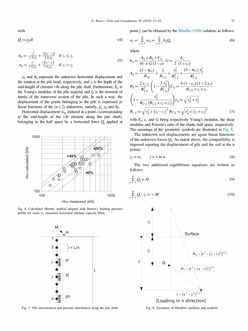
Eq. (2) by Barton (1984) producing the larger values. In Fig. 6, thecomparison between the experimental and the calculated values forthe horizontal ultimate capacity, Hlim, is repeated only for the caseof piles embedded in sand, adopting Barton’s pressure profile. Theagreement between the experimental and the calculated values isevidently improved as it emerges by the comparison between thediagram in Fig. 6 and the diagram in Fig. 5(b).

3.3. Boundary element method – computer program NAPHOL

The most conventional proposals for estimating the lateraldeflection and the bending moments of a laterally loaded singlepile or group of piles usually rely on either the theory of subgradereaction (Matlock and Reese, 1956) or the elastic continuumtheory, generally by the Boundary Element Method (Poulos, 1971)or the Finite Element Method (Yang and Jeremic, 2002), or evenon hybrid methods (Kitiyodom and Matsumoto, 2002; 2003). Theeffects of nonlinearity can be taken into account in the theory ofsubgrade reaction by introducing nonlinear spring characteristics.Such an approach leads to the development of the so-called”p–y”method by Reese et al. (1975). It is also possible to developnonlinear lateral response solutions from the elastic continuumtheory, by imposing the condition whereby lateral soil pressure pcannot exceed an ultimate value py (Davies and Budhu, 1986).A computer program, called NAPHOL (Landi, 2006), based

on BEM, has been developed. In this program, the pile ismodelled as a linearly elastic beam interacting with a linearlyelastic homogeneous and isotropic half space. The pile–soilinterface is discretized into n rectangular areas of width d andlength l¼L/n; the distribution of stress acting at the interface isapproximated (Fig. 7) by n values of horizontal normal stress puniformly distributed with constant intensity over each area.The problem is solved by equating the horizontal displacementof the pile to that of the half space, both calculated at the mid-height of each element as a function of the unknown stresses pi.Two further equations are obtained by imposing equilibriumbetween the external forces (horizontal load H and moment M)and the pressure distribution along the pile shaft.The horizontal displacement at the mid-height of pile

element i may be written as

yi ¼ � Σn

j ¼ 1αijQjþy0þθ0 Uzi ð3Þ

100

1000

100 1000

Hlim

calc

ulat

ed (k

N)

Hlim measured (kN)

+40%

-40%

±20%

b) sand) vs. measured horizontal ultimate capacity Hlim.

G. Russo / Soils and Foundations 56 (2016) 33–43 37

with

Qj ¼ pjdl ð4Þ

αij ¼ z3i3 EpIp

þ z2i zj� zið Þ2 EpIp

if zirzj

αij ¼ z3j3 EpIp

þ z2j zi� zjð Þ2 EpIp

if zi4zjð5Þ

y0 and θ0 represent the unknown horizontal displacement andthe rotation at the pile head, respectively, and zi is the depth of themid-height of element i-th along the pile shaft. Furthermore, Ep isthe Young's modulus of the pile material and Ip is the moment ofinertia of the transverse section of the pile. In such a way, thedisplacement of the points belonging to the pile is expressed aslinear functions of the (nþ2) unknowns, namely, pj, y0 and θ0.

Horizontal displacement wij, induced at a point i (correspondingto the mid-height of the i-th element along the pile shaft),belonging to the half space by a horizontal force Qj applied at

100

1000

100 1000

Hlim

calc

ulat

ed (k

N)

Hlim measured (kN)

+40%

±20%

-40%

Fig. 6. Calculated (Broms’ method adapted with Barton’s limiting pressureprofile for sand) vs. measured horizontal ultimate capacity Hlim.

MH

L

l = L/n

1

2

i

j

n

pi

pj

pn

Fig. 7. Pile discretisation and pressure distribution along the pile shaft.

point j, can be obtained by the Mindlin (1936) solution, as follows:

wi ¼ Σn

j ¼ 1wij ¼ Σ

n

j ¼ 1bijQj ð6Þ

where

bij ¼AijþBijþCij

16 π G 1�νð Þ G¼ Es

2 1þνsð Þ

Aij ¼3�4νsð ÞR1ij

þ 1R2 ij

þ x2ijR31 ij

þ 3�4νsð Þ x2ijR32 ij

Bij ¼ 2 cj ziR32 ij

1� 3 x2ijR22 ij

!Cij ¼ 4 1�νsð Þ 1�2 νsð Þ

R2 ijþziþcj

1� x2ijR2 ij R2 ijþcjþzi

� � !

rij ¼ffiffiffiffiffiffiffiffiffiffiffiffiffiffix2ijþy2ij

q

R1 ij ¼ffiffiffiffiffiffiffiffiffiffiffiffiffiffiffiffiffiffiffiffiffiffiffiffiffiffir2ijþ zi�cj

� �2qR2 ij ¼

ffiffiffiffiffiffiffiffiffiffiffiffiffiffiffiffiffiffiffiffiffiffiffiffiffiffir2ijþ ziþcj

� �2qð7Þ

with Es, νs and G being respectively Young’s modulus, the shearmodulus and Poisson’s ratio of the elastic half space, respectively.The meanings of the geometric symbols are illustrated in Fig. 8.The unknown soil displacements are again linear functions

of the unknown forces Qj. As stated above, the compatibility isimposed equating the displacement of pile and the soil at the npoints:

yi ¼ wi i¼ 1 to n ð8ÞThe two additional equilibrium equations are written as

follows:

Σn

j ¼ 1Qj ¼H ð9Þ

Σn

j ¼ 1Qj Uzj ¼ �M ð10Þ

Fig. 8. Geometry of Mindlin’s problem and symbols.

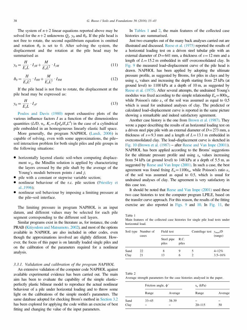
Table 1Main features of the collected case histories for single pile load tests underhorizontal load.

Soil type Number ofcases

Field test Centrifuge test ymax/D(range)

Steel pipepiles

R.C.piles

Sand 22 8 9 5 4–12%

G. Russo / Soils and Foundations 56 (2016) 33–4338

The system of nþ2 linear equations reported above may besolved for the nþ2 unknowns Qj, y0 and θ0. If the pile head isnot free to rotate, the second equilibrium equation is omittedand rotation θ0 is set to 0. After solving the system, thedisplacement and the rotation at the pile head may besummarised as

y0 ¼H

EsLU IyHþ M

EsL2U IyM ð11Þ

ϑ0 ¼ H

EsL2U IϑHþ M

EsL3U IϑM ð12Þ

If the pile head is not free to rotate, the displacement at thepile head may be expressed as:

y0 ¼H

EsLU IyF ð13Þ

Poulos and Davis (1980) report exhaustive plots of thevarious influence factors I as a function of the dimensionlessquantities (L/D, υs, Kr¼EpIp/EsL

4) in the case of a cylindricalpile embedded in an homogeneous linearly elastic half space.

More generally, the program NAPHOL (Landi, 2006) iscapable of solving, even with some approximations, the pile–soil interaction problem for both single piles and pile groups inthe following situations:

� horizontally layered elastic soil-when computing displace-ment wij, the Mindlin solution is applied by characterizingthe layers crossed by the pile shaft by the average of theYoung’s moduli between points i and j;

� pile with a constant or stepwise variable section;� nonlinear behaviour of the r.c. pile section (Priestley et

al.,1996);� nonlinear soil behaviour by imposing a limiting pressure at

the pile–soil interface.

The limiting pressure in program NAPHOL is an inputdatum, and different values may be selected for each pilesegment corresponding to the different soil layers.

Similar programs exist in the literature as, for instance, the codePRAB (Kitiyodom and Matsumoto, 2002), and most of the optionsavailable in NAPHOL are also included in other codes, eventhough the approximations involved are slightly different. How-ever, the focus of this paper is on laterally loaded single piles andon the calibration of the parameters required for a nonlinearanalysis.

Clay 21 13 6 2 3.5–16%

Table 2Average strength parameters for the case histories analysed in the paper.

Friction angle, ϕ1 su (kPa)

Range Average Range Average

Sand 33–45 38-39 – –

Clay – – 20–115 50

3.3.1. Validation and calibration of the program NAPHOLAn extensive validation of the computer code NAPHOL against

available experimental evidence has been carried out. The mainaim has been to evaluate the capability of the simple elastic–perfectly plastic bilinear model to reproduce the actual nonlinearbehaviour of a pile under horizontal loading and to throw somelight on the calibrations of the simple model’s parameters. Thesame database adopted for checking Brom’s method in Section 3.2has been explored for applying the code within an exercise of bestfitting and changing the value of the input parameters.

In Tables 1 and 2, the main features of the collected casehistories are summarised.Just two examples out of the many back analyses carried out are

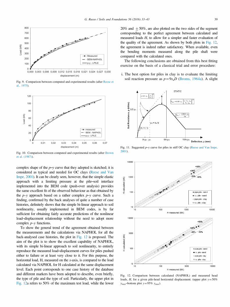
illustrated and discussed. Reese et al. (1975) reported the results ofa horizontal loading test on a driven steel tubular pile with anexternal diameter of D¼641 mm, a thickness of s¼12 mm and alength of L¼15.2 m embedded in stiff overconsolidated clay. InFig. 9 the measured load–displacement curve of the pile head isdrawn. NAPHOL has been applied by adopting the ultimatepressure profile, as suggested by Broms, for piles in clays and byusing su values and increasing the depth starting from 25 kPa (atground level) to 1100 kPa at a depth of 10 m, as suggested byReese et al. (1975). After several attempts, the undrained Young’smodulus was fixed according to the simple relationship Eu¼800su,while Poisson’s ratio νs of the soil was assumed as equal to 0,5which is usual for undrained analyses of clay. The predicted orcalculated load–displacement curve is reported in the same pictureshowing a remarkable and indeed satisfactory agreement.Another case history is the one from Brown et al. (1987). They

wrote a paper describing the results of an horizontal loading test ona driven steel pipe pile with an external diameter of D¼273 mm, athickness of s¼9.3 mm and a length of L¼13.1 m embedded inoverconsolidated clay. The load–displacement curve is sketched inFig. 10 (Brown et al. (1987) – after Reese and Van Impe (2001)).NAPHOL has been applied according to the Broms’ suggestionsfor the ultimate pressure profile and using su values increasingfrom 54 kPa (at ground level) to 148 kPa at a depth of 5.5 m, assuggested by Reese and Van Impe (2001). In such a case, the bestagreement was found fixing Eu¼1100su, while Poisson’s ratio νsof the soil was assumed as equal to 0.5, which is usual forundrained analyses of clay. The agreement is very satisfactory inthis case too.It should be noted that Reese and Van Impe (2001) used these

two case histories to test the computer program LPILE, based onthe transfer curve approach. For this reason, the results of the fittingexercise are also reported in Figs. 9 and 10. In Fig. 11, the

0

100

200

300

400

500

600

700

800

0,000 0,003 0,006 0,009 0,012 0,015 0,018 0,021 0,024 0,027 0,030

Load

(kN

)

displacement (m)

MeasuredBEM-NAPHOLp-y - LPILE

Fig. 9. Comparison between computed and experimental results (after Reese etal., 1975).

0

20

40

60

80

100

120

0 0,01 0,02 0,03 0,04 0,05 0,06 0,07

Load

(kN

)

displacement (m)

measuredBEM - NAPHOLp-y - LPILE

Fig. 10. Comparison between computed and experimental results (after Brownet al. (1987)).

Fig. 11. Suggested p–y curve for piles in stiff OC clay (Reese and Van Impe,2001).

Fig. 12. Comparison between calculated (NAPHOL) and measured headloads, H, for a given pile-head horizontal displacement. (upper plot y¼50%ymax–bottom plot y¼95% ymax).

G. Russo / Soils and Foundations 56 (2016) 33–43 39

complex shape of the p–y curve that they adopted is sketched; it isconsidered as typical and needed for OC clays (Reese and VanImpe, 2001). It can be clearly seen, however, that the simple elasticapproach with a limiting pressure at the pile–soil interfaceimplemented into the BEM code (push-over analysis) providesthe same excellent fit of the observed behaviour as that obtained bythe p–y approach based on a rather complex p–y curve. Such afinding, confirmed by the back analyses of quite a number of casehistories, definitely shows that the simple bi-linear approach to soilnonlinearity, usually implemented in BEM codes, is by farsufficient for obtaining fairly accurate predictions of the nonlinearload–displacement relationship without the need to adopt morecomplex p–y functions.

To show the general trend of the agreement obtained betweenthe measurements and the calculations via NAPHOL for all theback-analysed case histories, the plot in Fig. 12 is proposed. Theaim of the plot is to show the excellent capability of NAPHOL,with its simple bi-linear approach to soil nonlinearity, to entirelyreproduce the measured load–displacement curves for piles pushedeither to failure or at least very close to it. For this purpose, thehorizontal load, H, measured on the x-axis, is compared to the loadcalculated via NAPHOL for H calculated at the same displacementlevel. Each point corresponds to one case history of the databaseand different markers have been adopted to describe, even briefly,the type of pile and the type of soil. Particularly, the upper plot inFig. 12a refers to 50% of the maximum test load, while the lower

20% and 750%, are also plotted on the two sides of the segmentcorresponding to the perfect agreement between calculated andmeasured loads H, to allow for a simpler and faster evaluation ofthe quality of the agreement. As shown by both plots in Fig. 12,the agreement is indeed rather satisfactory. When available, eventhe bending moments measured along the pile shaft werecompared with the calculated ones.The following conclusions are obtained from this best fitting

exercise on the basis of a classical trial and error procedure:

i. The best option for piles in clay is to evaluate the limitingsoil reaction pressure as p¼9suD (Broms, 1964a). A slight

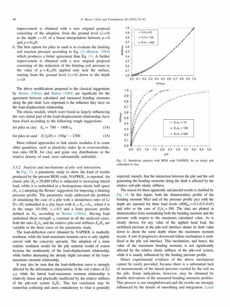
Fig. 13. Sensitivity analysis with BEM code NAPHOL for an elastic pileembedded in clay.

G. Russo / Soils and Foundations 56 (2016) 33–4340

improvement is obtained with a new original proposalconsisting of the adoption, from the ground level (z¼0)to the depth z¼D, of a linear interpolation between p¼0and p¼9suD;

ii. The best option for piles in sand is to evaluate the limitingsoil reaction pressure according to Eq. (2) (Barton, 1984)which produces a better agreement than Eq. (1). A furtherimprovement is obtained with a new original proposalconsisting of the reduction of the limiting soil pressure tothe value of p¼KpγDz applied only near the surface,starting from the ground level (z¼0) down to the depthz¼D.

The above modifications proposed to the classical suggestionsby Broms (1964a) and Barton (1984) are significant for theagreement between calculated and measured bending momentsalong the pile shaft. Less important is the influence they have onthe load–displacement relationship.

The elastic moduli, which were found as largely influencingthe very initial part of the load–displacement relationship, havebeen fixed according to the following rough suggestions:

for piles in clay Eu ¼ 700� 1400 su ð14Þ

for piles in sand E= γDð Þ ¼ 150φ1� 2300 ð15ÞMore refined approaches to link elastic modulus E to some

other quantities, such as plasticity index Ip or overconsolida-tion ratio OCR, for clay and grain size distributions or therelative density of sand, were substantially unfruitful.

3.3.2. Analysis and mechanisms of pile–soil interaction.In Fig. 13, a parametric study to show the kind of results

produced by the present BEM code, NAPHOL, is reported. Anelastic pile (Ep¼28,000 GPa) is subjected to increasing lateralload, while it is embedded in a homogenous elastic half space(Es, νs) adopting the Broms’ suggestion for imposing a limitingpressure profile. The parametric study addressed the problemof simulating the case of a pile with a slenderness ratio of L/D¼20, embedded in a clay layer with Es¼Eu¼ksu, where k isin the range 10–500, vs¼0.5 and a limit pressure profiledefined as 9su according to Broms (1964a). Having keptundrained shear strength su constant in all the analysed cases,both the ratio Eu/su and the relative pile–soil stiffness Ep/Eu arevariable in the three cases of the parametric study.

The load–deflection curve obtained by NAPHOL is markedlynonlinear, while the load–maximum moment curve is only slightlycurved with the concavity upwards. The adoption of a morerealistic nonlinear model for the pile material would of courseincrease the nonlinearity of the load–displacement relationship,while further attenuating the already slight curvature of the load–maximum moment relationship.

It may also be seen that the load–deflection curve is stronglyaffected by the deformation characteristic of the soil (values of Es/su), while the lateral load–maximum moment relationship isrelatively linear and practically unaffected by the relative stiffnessof the pile–soil system Ep/Es. This last conclusion may besomewhat confusing and seem contradictory to what is generally

expected, namely, that the interaction between the pile and the soilgenerating the bending moments along the shaft is affected by therelative soil–pile elastic stiffness.The reason for these apparently unexpected results is clarified by

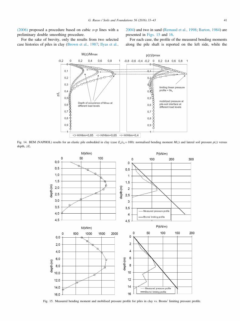
Fig. 14. In this figure, both the dimensionless profile of thebending moment M(z) and of the pressure profile p(z) with thedepth are reported for three load levels (H/Hlim¼0.3–0.5–0.65)and refer to the case of Es/su¼100. The data are plotted indimensionless form normalising both the bending moment and thepressure with respect to the maximum calculated value. As isclearly shown, for any value of the applied head load, themobilised pressure at the pile–soil interface attains its limit valuedown to about the same depth where the maximum momentoccurs. A sort of progressive downward failure mechanism is mob-ilised at the pile soil interface. This mechanism, and hence, thevalue of the maximum bending moment, is not significantlyaffected by the relative elastic stiffness of the pile–soil system,while it is mainly influenced by the limiting pressure profile.Direct experimental evidence of the above mechanism

cannot be easily provided, because there is a substantial lackof measurements of the lateral pressure exerted by the soil onthe pile. Some indications, however, may be obtained bydouble derivations of the measured bending moments profiles.This process is not straightforward and the results are stronglyinfluenced by the details of smoothing and integration. Landi

G. Russo / Soils and Foundations 56 (2016) 33–43 41

(2006) proposed a procedure based on cubic s–p lines with apreliminary double smoothing procedure.

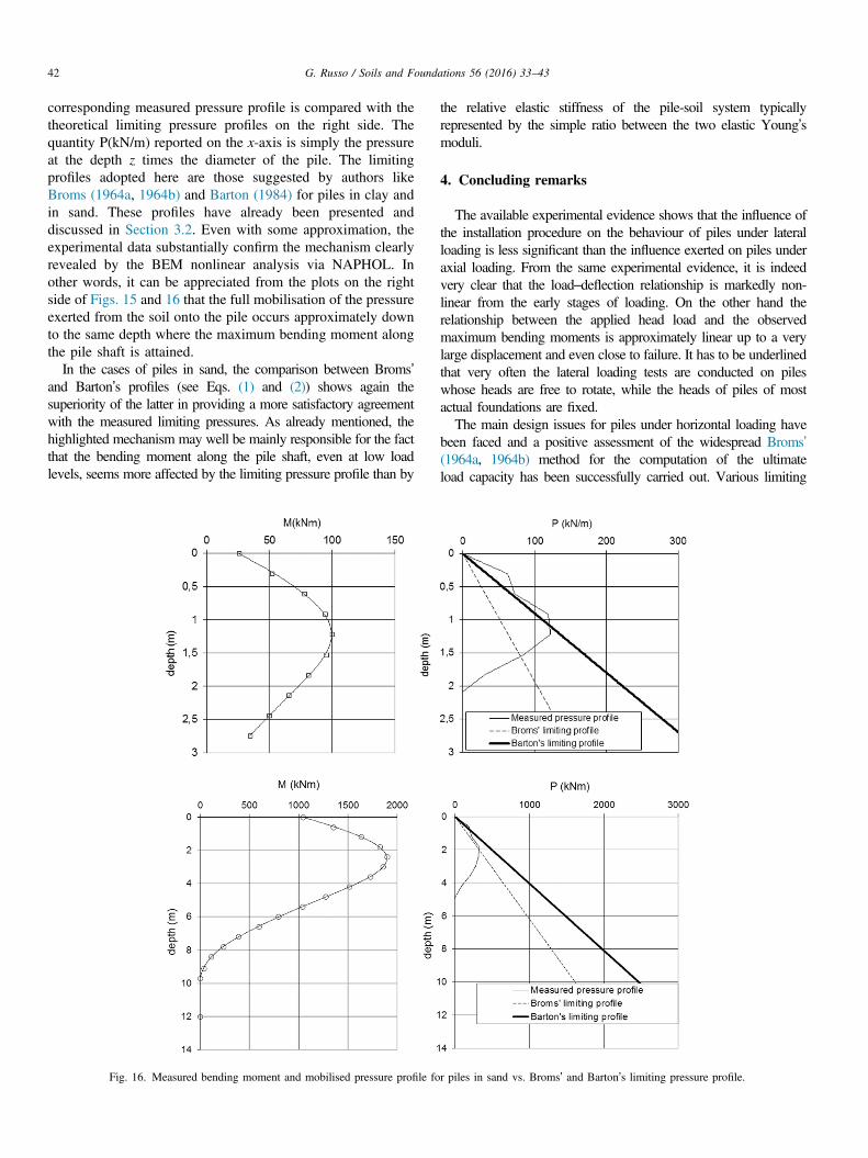
For the sake of brevity, only the results from two selectedcase histories of piles in clay (Brown et al., 1987; Ilyas et al.,

Fig. 14. BEM (NAPHOL) results for an elastic pile embedded in clay (case Eu/sudepth, z/L.

Fig. 15. Measured bending moment and mobilised pressure pr

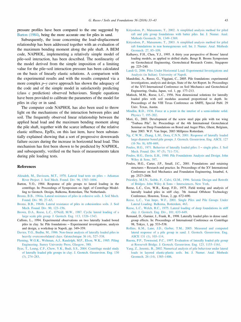
2004) and two in sand (Remaud et al., 1998; Barton, 1984) arepresented in Figs. 15 and 16.For each case, the profile of the measured bending moments

along the pile shaft is reported on the left side, while the

¼100): normalised bending moment M(z) and lateral soil pressure p(z) versus

ofile for piles in clay vs. Broms’ limiting pressure profile.

G. Russo / Soils and Foundations 56 (2016) 33–4342

corresponding measured pressure profile is compared with thetheoretical limiting pressure profiles on the right side. Thequantity P(kN/m) reported on the x-axis is simply the pressureat the depth z times the diameter of the pile. The limitingprofiles adopted here are those suggested by authors likeBroms (1964a, 1964b) and Barton (1984) for piles in clay andin sand. These profiles have already been presented anddiscussed in Section 3.2. Even with some approximation, theexperimental data substantially confirm the mechanism clearlyrevealed by the BEM nonlinear analysis via NAPHOL. Inother words, it can be appreciated from the plots on the rightside of Figs. 15 and 16 that the full mobilisation of the pressureexerted from the soil onto the pile occurs approximately downto the same depth where the maximum bending moment alongthe pile shaft is attained.

In the cases of piles in sand, the comparison between Broms’and Barton’s profiles (see Eqs. (1) and (2)) shows again thesuperiority of the latter in providing a more satisfactory agreementwith the measured limiting pressures. As already mentioned, thehighlighted mechanism may well be mainly responsible for the factthat the bending moment along the pile shaft, even at low loadlevels, seems more affected by the limiting pressure profile than by

Fig. 16. Measured bending moment and mobilised pressure profile fo

the relative elastic stiffness of the pile-soil system typicallyrepresented by the simple ratio between the two elastic Young’smoduli.

4. Concluding remarks

The available experimental evidence shows that the influence ofthe installation procedure on the behaviour of piles under lateralloading is less significant than the influence exerted on piles underaxial loading. From the same experimental evidence, it is indeedvery clear that the load–deflection relationship is markedly non-linear from the early stages of loading. On the other hand therelationship between the applied head load and the observedmaximum bending moments is approximately linear up to a verylarge displacement and even close to failure. It has to be underlinedthat very often the lateral loading tests are conducted on pileswhose heads are free to rotate, while the heads of piles of mostactual foundations are fixed.The main design issues for piles under horizontal loading have

been faced and a positive assessment of the widespread Broms’(1964a, 1964b) method for the computation of the ultimateload capacity has been successfully carried out. Various limiting

r piles in sand vs. Broms’ and Barton’s limiting pressure profile.

G. Russo / Soils and Foundations 56 (2016) 33–43 43

pressure profiles have been compared to the one suggested byBarton (1984), being the more accurate one for piles in sand.

Subsequently, the issue concerning the load–displacementrelationship has been addressed together with an evaluation ofthe maximum bending moment along the pile shaft. A BEMcode, NAPHOL, implementing a relatively simple model ofpile–soil interaction, has been described. The nonlinearity ofthe model derived from the simple imposition of a limitingvalue for the pile–soil interaction pressure has been calculatedon the basis of linearly elastic solutions. A comparison withthe experimental results and with the results computed via amore complex p–y curve approach has shown the adequacy ofthe code and of the simple model in satisfactorily predicting(class c prediction) observed behaviours. Simple equationshave been provided to calibrate the parameters of the model forpiles in clay or in sand.

The computer code NAPHOL has also been used to throwlight on the mechanisms of the interaction between piles andsoil. The frequently observed linear relationship between theapplied head load and the maximum bending moment alongthe pile shaft, together with the scarce influence of the relativeelastic stiffness, Ep/Es, on this last item, have been substan-tially explained showing that a sort of progressive downwardsfailure occurs during the increase in horizontal head load. Thismechanism has first been shown to be predicted by NAPHOL,and subsequently, verified on the basis of measurements takenduring pile loading tests.

References

Alizadeh, M., Davisson, M.T., 1970. Lateral load tests on piles – ArkansasRiver Project. J. Soil Mech. Found. Div. 96, 1583–1604.

Barton, Y.O., 1984. Response of pile groups to lateral loading in thecentrifuge. In: Proceedings of Symposium on Appl. of Centrifuge Model-ling to Geotech. Design, Balkema, Rotterdam, The Netherlands.

Broms, B.B., 1964a. Lateral resistance of piles in cohesive soils. J. Soil Mech.Found. Div. 90, 27–63.

Broms, B.B., 1964b. Lateral resistance of piles in cohesionless soils. J. SoilMech. Found. Div. 90, 123–156.

Brown, D.A., Reese, L.C., O’Neill, M.W., 1987. Cyclic lateral loading of alarge scale pile group. J. Geotech. Eng. 113, 1326–1343.

Callisto, L., 1994. Experimental observations on two laterally loaded boredpiles in clay. In: Pile foundations – Experimental investigations, analysisand design, a workshop in Napoli, pp. 349–359.

Davies, T.G., Budhu, M., 1986. Non-linear analysis of laterally loaded piles inheavily overconsolidated clays. Géotechnique 36 (4), 527–538.

Fleming, W.G.K., Weltman, A.J., Randolph, M.F., Elson, W.K., 1985. PilingEngineering. Surrey University Press, Glasgow, 380.

Ilyas, T., Leung, C.F., Chow, Y.K., Budi, S.S., 2004. Centrifuge model studyof laterally loaded pile groups in clay. J. Geotech. Geoenviron. Eng. 130(3), 274–283.

Kitiyodom, P., Matsumoto, T., 2002. A simplified analysis method for piledraft and pile group foundations with batter piles. Int. J. Numer. Anal.Methods Geomech. 26, 1349–1369.

Kitiyodom, P., Matsumoto, T., 2003. A simplified analysis method for piledraft foundations in non homogeneous soil. Int. J. Numer. Anal. MethodsGeomech. 27, 85–109.

Kulhawy, F.H., Chen, Y.J., 1995. A thirty year perspective of Broms’ lateralloading models, as applied to drilled shafts. Bengt B. Broms Symposiumon Geotechnical Engineering, Geotechnical Research Centre, Singaporepp. 225–240.

Landi G, 2006. Piles Under Horizontal Load: Experimental Investigations andAnalysis (in Italian). University of Napoli.

Mandolini, A., Russo, G., Viggiani, C., 2005. Pile foundations: experimentalinvestigations, analysis and design, State of the Art Report. In: Proceedingsof the XVI International Conference on Soil Mechanics and GeotechnicalEngineering, Osaka, Japan, vol. 1, pp. 177–213.

Matlock, M.M., Reese, L.C., 1956. Non dimensional solutions for laterallyloaded piles with soil modulus assumed proportional to depth. In:Proceedings of the VIII Texas Conference on SMFE, Special Publ. 29Univ. Texas, Austin.

Mindlin, R.D., 1936. Force at a point in the interior of a semi-infinite solid.Physics 7, 195–202.

Mori, G., 2003. Development of the screw steel pipe pile with toe wing“Tsubasa Pile”. In: Proceedings of the 4th International GeotechnicalSeminar on Deep Foundations on Bored and Auger Piles, Ghent, Belgium,June 2003. W.F. Van Impe, 2003 Millpress Rotterdam.

Ng, C.W.W., Zhang, L.M., Dora, C.N.N, 2001. Response of laterally loadedlarge-diameter bored pile groups. J. Geotech. Geoenviron. Eng. ASCE. 127(16 No. 8), 658–669.

Poulos, H.G., 1971. Behavior of laterally loaded piles: I – single piles. J. SoilMech. Found. Div. 97 (5), 711–731.

Poulos, H.G., Davis, E.H., 1980. Pile Foundations Analysis and Design. JohnWiley & Sons, 397.

Poulos, H.G., Carter, J.P., Small, J.C., 2001. Foundations and retainingstructures – Research and practice. In: Proceedings of the XV InternationalConference on Soil Mechanics and Foundation Engineering, Istanbul, 4,pp. 2527–2606.

Priestley, M.J.N., Seible, F., Calvi, Gl.M., 1996. Seismic Design and Retrofitof Bridges. John Wiley & Sons – Intersciences, New York.

Reese, L.C., Cox, W.R., Koop, F.D., 1975. Field testing and analysis oflaterally loaded piles in stiff clay. 7th Annual Offshore TechnologyConference, Houston, Texas, 2, pp. 672–690.

Reese, L.C., Van Impe, W.F., 2001. Single Piles and Pile Groups UnderLateral Loading. Balkema, Rotterdam, 463.

Reese, L.C., Welch, R.C., 1975. Lateral loading of deep foundations in stiffclay. J. Geotech. Eng. Div., 101; 633–649.

Remaud, D., Garnier, J., Frank, R., 1998. Laterally loaded piles in dense sand:group effects. In: Proceedings of International Conference on Centrifuge98, Tokyo, 1, pp. 533–538.

Rollins, K.M., Lane, J.D., Gerber, T.M., 2005. Measured and computedlateral response of a pile group in sand. J. Geotech. Geoenviron. Eng.ASCE 131 (1), 103–114.

Ruesta, P.F., Townsend, F.C., 1997. Evaluation of laterally loaded pile groupat Roosevelt Bridge. J. Geotech. Geoenviron. Eng. 123, 1153–1161.

Yang, Z., Jeremic, B., 2002. Numerical analysis of pile behaviour under lateralloads in layered elastic-plastic soils. Int. J. Numer. Anal. MethodsGeomech. 26 (14), 1385–1406.