Embed Size (px)
Citation preview

A METHOD OF DECOUPLING OF RADIOFREQUENCY COILS IN MAGNETIC
RESONANCE IMAGING: APPLICATION TOMRI WITH ULTRA SHORT ECHO TIMEAND CONCURRENT EXCITATION AND
ACQUISITION
a thesis
submitted to the department of electrical and
electronics engineering
and the graduate school of engineering and science
of bilkent university
in partial fulfillment of the requirements
for the degree of
master of science
By
Ali Caglar Ozen
May, 2013

I certify that I have read this thesis and that in my opinion it is fully adequate,
in scope and in quality, as a thesis for the degree of Master of Science.
Prof. Dr. Ergin Atalar(Advisor)
I certify that I have read this thesis and that in my opinion it is fully adequate,
in scope and in quality, as a thesis for the degree of Master of Science.
Prof. Dr. Yusuf Ziya Ider
I certify that I have read this thesis and that in my opinion it is fully adequate,
in scope and in quality, as a thesis for the degree of Master of Science.
Prof. Dr. Murat Eyuboglu
Approved for the Graduate School of Engineering and Science:
Prof. Dr. Levent OnuralDirector of the Graduate School
ii
ABSTRACT
A METHOD OF DECOUPLING OF RADIOFREQUENCY COILS IN MAGNETIC RESONANCEIMAGING: APPLICATION TO MRI WITH ULTRA
SHORT ECHO TIME AND CONCURRENTEXCITATION AND ACQUISITION
Ali Caglar Ozen
M.S. in Electrical and Electronics Engineering
Supervisor: Prof. Dr. Ergin Atalar
May, 2013
In this thesis, it was both experimentally and theoretically shown that decoupling
of transmit and receive coils can be achieved by using a transmit array system
such that individual currents induced from transmit coils will cancel each other
resulting in a significantly reduced coupling. A novel method for decoupling of
radio frequency (RF) coils was developed and implemented in a transmit array
system with multiple transmit coil elements driven by RF current sources of differ-
ent amplitude and phase. It was shown that this method for decoupling provides
isolation over 70dB between transmit and receive coils. Decoupling procedure
was described and its performance was analyzed in terms of obtained isolation.
It was shown that MR signal can be detected during RF excitation with the
achieved amount of decoupling. NMR spectroscopy and MRI with concurrent
excitation and acquisition (CEA) was implemented. As an alternative to existing
CEA methods, this method reduces dynamic range requirements so that CEA
sequences can be applied in standard MRI scanners with minimal hardware mod-
ification. It was also demonstrated that this method can be used to implement
ultra-short echo time (UTE) imaging with shorter acquisition delay. For CEA
approach, acquired raw data was formulated as convolution of the free induction
decay (FID) signal and the input B1 field. First proof of concept images were re-
constructed from nonuniformly sampled k space data using both UTE and CEA
sequences. UTE and CEA were shown to be feasible to implement using the
same custom made decoupling setup in a clinical 3T MRI scanner. Significance
of imaging of samples with ultra short T2* values was discussed.
Keywords: MRI, Continuous-wave NMR, CEA, UTE, transmit array, decoupling.
iii

OZET
MANYETIK REZONANS GORUNTULEMEDE RADYOFREKANS SARGILARININ IZOLASYONU ICIN BIR
YONTEM: ES ZAMANLI RF UYARIMI VE COK KISAYANKI SURELI MRG’YE UYGULANMASI
Ali Caglar Ozen
Elektrik ve Elektronik Muhendisligi, Yuksek Lisans
Tez Yoneticisi: Prof. Dr. Ergin Atalar
Mayıs, 2013
Bu tezde, alıcı ve verici sargılar arasındaki izolasyonun verici dizisi kullanılarak,
dizi elemanlarının olusturdugu akımlar birbirini yok edecek sekilde surulmesiyle
gercklestirilebilecegi deneysel ve teorik olarak gosterildi. Bu izolasyon yontemi,
paralel verici dizisi kullanılarak dizi elemanlarının farklı genlik ve fazlara sahip
radyo frekans (RF) akımlarıyla surulmesiyle gerceklestirilmistir. Bu yontemle
alıcı ve verici sargılar arasında 70dB uzerinde izolasyon elde edilebilecegi
gosterildi. Izolasyon yontemi ayrıntılı bir sekilde anlatılarak elde edilen izo-
lasyon uzerinden performans analizi yapıldı. Elde edilen izolasyon ile MR
sinyalinin RF uyarımı sırasında gozlenebilecegi gosterildi. Nukleer manyetik re-
zonans spektroskopi ve manyetik rezonans goruntuleme es zamanlı uyarım ve
sinyal kaydı yontemiyle gerceklestirildi. Bu sayede dinamik erim gereksinim-
leri azaltılarak standart MRG cihazlarında es zamanlı uyarım ve data alımının
gerceklestirilebilecegi gosterildi. Bu izolasyon yonteminin, cok kısa yankı sureli
MRG tekniklerinin uygulanmasındaki data kayıt erteleme suresinin azaltılması
icin de kullanılabilecegi gosterildi. Es zamanlı uyarım MRG teknigi icin
kaydedilen sinyal, goruntulenen nesnenin izdusumu ile RF sinyalinin evrilmesi
olarak formule edildi. Isınsal k uzayı tarama yontemi ile elde edilen goruntulerle,
es zamanlı uyarım ve cok kısa yankı sureli MRG tekniklerinin tasarlanan izo-
lasyon duzenegi ile gerceklestirilebilecegi gosterildi. Cok kısa T2* sureli dokuların
goruntulenmesinin onemi MRG teknikleri uzerinden tartısıldı.
Anahtar sozcukler : MRG, Surekli-uyarım NMR, es zamanlı uyarım ve data kaydı,
cok kısa yankı sureli goruntuleme, verici dizisi, izolasyon.
iv

Acknowledgement
Apart from my own efforts, existence of this thesis depends largely on the en-
couragement and guidelines of many others:
First of all, I would like to express my deep gratitude to Prof. Dr. Ergin Atalar
who made this thesis, and many other valuable works, possible by providing ex-
cellent supervision and a great research opportunity being the founder and the
director of the National Magnetic Resonance Research Center (UMRAM). And I
would like to thank him for giving a great deal of trust in my research capabilities,
encouraging me at every step and for his endless enthusiasm and patience.
I thank Prof. Dr. Yusuf Ziya Ider and Prof. Dr. Murat Eyuboglu for showing
interest in my work and allocating their precious time to read and giving critical
comments on this thesis.
I would also like to mention my colleagues in UMRAM and my friends Taner
Demir, Volkan Acıkel, Ugur Yılmaz, Can Kerse, Emre Kopanoglu, Esra Abacı
Turk, Aydan Ercingoz, Yigitcan Eryaman, Ibrahim Mahcicek, Yıldıray Gokhalk,
Koray Ertan, Umut Gundogdu, Cemre Arıyurek, Dr. Oktay Algın for their men-
tal and physical supports during my graduate school adventure. Especially Burak
Akın, for sitting up together almost all the summer nights studying in UMRAM.
Finally, I will always be grateful for the unconditional supports of Semra, Hidayet
and my little brother Hasan. They have always been a friendly, and understand-
ing family whatever the choices I make in life.
I am also indebted to Ugur Erdem, my lifelong mentor for even his existence
makes me a stronger person.
v

Contents
1 Introduction 1
2 Material and Methods 6
2.1 Decoupling of RF Coils . . . . . . . . . . . . . . . . . . . . . . . . 6
2.2 Application to UTE . . . . . . . . . . . . . . . . . . . . . . . . . . 13
2.3 Application to CEA . . . . . . . . . . . . . . . . . . . . . . . . . . 16
3 Results 28
3.1 Decouping of RF Coils . . . . . . . . . . . . . . . . . . . . . . . . 28
3.2 Application to UTE . . . . . . . . . . . . . . . . . . . . . . . . . . 33
3.3 Application to CEA . . . . . . . . . . . . . . . . . . . . . . . . . . 35
4 Discussions 44
5 Conclusions 48
A Measurement of Dielectric Properties 56
A.1 Introduction . . . . . . . . . . . . . . . . . . . . . . . . . . . . . . 57
vi

CONTENTS vii
A.2 Theory . . . . . . . . . . . . . . . . . . . . . . . . . . . . . . . . . 58
A.3 Material and Methods . . . . . . . . . . . . . . . . . . . . . . . . 58
A.4 Results . . . . . . . . . . . . . . . . . . . . . . . . . . . . . . . . . 62
A.5 Conclusions . . . . . . . . . . . . . . . . . . . . . . . . . . . . . . 64

List of Figures
2.1 Visual presentation of magnetic field lines for geometrical decou-
pling of two coils and the rotation setup we have built to implement
such an orthogonal placement by rotating receive coil around the
one of the transmit array coils conveniently with fine precision. . . 8
(a) Magnetic field lines . . . . . . . . . . . . . . . . . . . . . . . 8
(b) Rx coil rotation setup . . . . . . . . . . . . . . . . . . . . . 8
2.2 Visualization of decoupling process. First, Tx coil-1 and receive
coil are placed orthogonally which reduces the B1 induced current
on the receive coil as well as the transmit noise coupled current. Tx
coil-1 is driven by a current ITx1 inducing IRx1 on the receive coil.
Amplitude and phase of Tx coil-2 is adjusted such that IRx2 cancels
IRx1 out which reduces the total B1 induced voltage VRx by a
significant amount. Since ITx1 is greater than ITx2 by the amount of
the geometrical decoupling, the spins of the sample excited mostly
due to magnetic field produced by Tx coil-1. . . . . . . . . . . . 9
viii

LIST OF FIGURES ix
2.3 Schematic for the system setup. Transmit Array control unit con-
trols the amplitude and phase as well as the envelopes of the RF
waveforms via modulator. One of the outputs of the modulators
are amplified by an LNA while the other one is attenuated by an
RF attenuator in order to make B1 induced amplitudes of two
transmit coils comparable to each other. Oscilloscope is used to
check voltage levels at the modulator outputs and at the receive
coil output real time. Once the signal voltage level at the receive
coil output reduced to a value that would not saturate the receiver
circuitry of the scanner, we connect our receive coil to the scanner
via an ultra low noise amplifier. . . . . . . . . . . . . . . . . . . . 10
2.4 Circuit diagram and s parameters with noise figure and stability
factor of the amplifier used in the experiments. Single stage am-
plifier is built with a BFG135 bipolar transistor with input and
output matchings are performed. . . . . . . . . . . . . . . . . . . 21
(a) Circuit diagram of the LNA . . . . . . . . . . . . . . . . . . 21
(b) S parameters, Noise figure and Stability Factor . . . . . . . 21
2.5 Distortions on the output waveforms of the original 4kW system
RF power amplifiers measured with oscilloscope. System RFPAs
are driven by input RF signal amplitude of which is set to zero
from MR console. Nonlinear effects of the amplifiers are observed
as 400mVpp fluctuation signals. . . . . . . . . . . . . . . . . . . . . 22
2.6 The peaks are observed at the end of signal envelope due to a delay
about 10µs between transmit channels. This effect is eliminated in
the CEA experiments by starting acquisition 100µs later than RF
starts. . . . . . . . . . . . . . . . . . . . . . . . . . . . . . . . . . 23
2.7 System with a thermal noise source, and two active components. . 23
2.8 Experimental setup with a 8 channel birdcage transmit and a re-
ceive loop coil. A rubber phantom is placed on the receive coil. . . 23

LIST OF FIGURES x
2.9 Demonstration of decoupling when B1 induced voltage signal has
a time dependence. Transmit sinc pulse with a single side lobe
(a). Spectrum of the sinc pulse (b). Frequency response of the
decoupling system in 1024Hz range (c). Required transmit pulse
for better decoupling than decoupling using the same pulse trans-
mitted from both sources (d). . . . . . . . . . . . . . . . . . . . . 24
2.10 Calculation of the sampling density for a projection raw data set. 24
2.11 Nonuniformly sampled data is transformed into Cartesian grid
points. Value of a grid point is assigned by interpolation. . . . . . 25
2.12 Pulse sequence diagram for CEA with 128 radial projections and
a single time of repetition (TR) interval. . . . . . . . . . . . . . . 25
(a) UTE pulse sequence diagram for radial k space trajectory . 25
(b) Pulse sequence diagram for a single TR . . . . . . . . . . . . 25
2.13 T2* correction combined with apodization correction and addi-
tional constant. The correction function was determined experi-
mentally by trial and error method once we measure the T2* of the
sample as 450µs with a UTE relaxation sequence. Each raw FID
signal is multiplied with this correction function for enhancement
of high frequency information. . . . . . . . . . . . . . . . . . . . . 26
2.14 Transverse magnetization during rectangular B1 excitation calcu-
lated from Bloch equation under small tip angle assumption for a
sample with T2 of 1ms. . . . . . . . . . . . . . . . . . . . . . . . . 26
2.15 Sample pulse sequence diagram representing excitation, acquisi-
tion and encoding timings and magnitudes for a single TR inter-
val. Gradients along with the sweep range determine the FOV
and resolution. Changing the orientation of the gradients means
acquiring projections along various directions. . . . . . . . . . . . 27

LIST OF FIGURES xi
3.1 B1 induced voltage is measured for rotation of the receive coil
plane with respect to one of the transmit coils covering 180o. Ideal
linearly polarized field is calculated and both normalized to 0o to
impress the effect of getting closer to ideal condition. The limi-
tation in this task is that individual polarizations of the transmit
coils are slightly elliptically polarized. One should also consider
physical dimension of the coils and the distance between them be-
cause receive coil can affect the loading of transmit coil when they
are placed too close to each other and their physical dimensions
are similar, due to strong mutual coupling. . . . . . . . . . . . . 29
3.2 Decoupling versus Phase of an RF generator unit. Two-port decou-
pling is represented by changing the phase of one port in uniform
steps covering 360o. Data are normalized to 0o. Limitations of
decoupling using this procedure arises from the precision of the
phase control unit. Stability of the RF generator unit is also a
key factor for the achieved decoupling to be preserved during the
experiment. Addition of a third coil could increase the amount
of total decoupling which could be used to cancel remaining B1
current on the receive coil. . . . . . . . . . . . . . . . . . . . . . 30
3.3 B1 induced voltage signal in the receive coil after decoupling. Mul-
tiport decoupling without geometric decoupling (a), Multiport de-
coupling with 10dB geometric decoupling (b), Multiport decou-
pling with 20dB geometric decoupling (c). . . . . . . . . . . . . . 31
3.4 B1 induced voltage signals in the receive coil for single channel
transmission with varying input levels by changing the amplitude
scale of a chirp RF signal spanning -8kHz to 8kHz over 8ms from
Tx array user interface (a). Estimated system response for actual
input level (b). Estimated RF waveform to be transmitted from
the decoupling coil i.e. Tx coil-2 (c). . . . . . . . . . . . . . . . . 32

LIST OF FIGURES xii
3.5 B1 induced voltage signal in the receive coil after decoupling with
the same RF waveform transmitted from both transmit channels
(a), and a different RF waveform transmitted from the decoupling
coil as shown in Figure 3.4c (b). . . . . . . . . . . . . . . . . . . 33
3.6 Rubber phantom with holes (a). UTE image for 128 projections
and 30V peak RF input voltage (b). . . . . . . . . . . . . . . . . . 34
3.7 Demonstration of the T2* correction effects on the UTE signal of
a rubber sample: FID (a) and projection (b) enhancement using
T2* correction as defined in Chapter 2. . . . . . . . . . . . . . . . 35
3.8 UTE image of a rubber sample for 768 projections, 240V peak RF
input voltage and acquisition delay of 20µs without (a) and with
T2* correction (b). . . . . . . . . . . . . . . . . . . . . . . . . . . 36
3.9 UTE image for 768 projections, 240V peak RF input voltage and
acquisition delay of 20µs (a), 80µs (b), 120µs (c) and 200µs (d) . . 37
3.10 B1 map generated with Bloch-Siegert shift method for 20Vpeak
Fermi RF pulse with 4kHz off resonance. Decoupling setup is used
with a rubber inside the glass of tap water phantom. Average B1
value is calculated as 4µT. Phase image out of the Gradient Echo
based Bloch-Siegert shift sequence (a), phase image after unwrap-
ping process (b), and calculated |B1| map with masking applied
(c). . . . . . . . . . . . . . . . . . . . . . . . . . . . . . . . . . . . 38
3.11 Concurrent MR signal acquired using 3T transmit array system
with TR=1000 ms, Resolution =512, Acquisition BW: 50Hz/Px.
This data is unprocessed raw data including B1 induced voltage
signal remaining after decoupling. If leakage is higher the oscilla-
tions due to magnetization induced signal would be invisible. Since
there is no gradient applied, the signal is accumulated all over the
sample volume. . . . . . . . . . . . . . . . . . . . . . . . . . . . . 39

LIST OF FIGURES xiii
3.12 Concurrent MR signal acquired with 20mT/m slice selection gra-
dient turned on at t=4ms. Turn on of gradient causes the signal
level to drop immediately. The space encoded information can be
extracted with weaker gradients and higher B1 applied. In this
experiment, the input RF power was 0.8mW . . . . . . . . . . . 40
3.13 Raw data out of a CEA experiment for chirp B1 excitation of
±500Hz over 40ms observed in water phantom. . . . . . . . . . . 40
3.14 Acquired raw data from a water sample (a). Input B1 waveform as
a chirp function (b). Acquired signal after the leakage subtraction
(c). Fourier transform of the estimated FID signal after deconvo-
lution (d) and single-sided FID signal which is an approximation
of the actual FID (e). . . . . . . . . . . . . . . . . . . . . . . . . . 41
3.15 Raw data acquired from ethanol sample (a). Chemical shift spec-
trum obtained after deconvolution (b). . . . . . . . . . . . . . . . 42
3.16 Rubber phantom of T2 of 500µs with holes (a). CEA image (b). . 42
3.17 Rubber phantom of T2 of 500µs with holes (a). CEA image with
improved imaging parameters and gridding with Keiser-Bessel in-
terpolation (b), and T2* correction applied (c). . . . . . . . . . . 42
3.18 B1 induced leakage signal variation over subsequent measurements
after decoupling is preceeded. The measurements are taken subse-
quently with 1min intervals while keeping everything unchanged. . 43
A.1 Schematic of coaxial fixture. The transmission line is modeled
as two series lumped element model of a coaxial line one which
has a lossy medium inside while the other one is filled with air.
Dimensions are given. The length vector of pouring the sample
inside the fixture is calculated and entered in the optimization
program as input along with the measured reflection coefficient data. 59

LIST OF FIGURES xiv
A.2 Realistic model of the fixture is created using ADS R©. Physical
dimensions are measured with high precision micrometers. The
part of the fixture that is filled with derlin is also considered in this
model. Test for the optimization program written in MATLAB R© is
done using s-parameter simulations out of the ADS R© using realistic
model. . . . . . . . . . . . . . . . . . . . . . . . . . . . . . . . . . 60
A.3 Picture of experimental setup. The collection of data is done as
follows. First the network analyzer is calibrated properly in a
desired frequency range taking the impedance of the empty fixture
into account. Test phantom is prepared and samples are gathered
using a pipette and poured into the fixture in desired amount.
At each step the reflection coefficients are recorded. In recent
measurements an automatic pipette is used which is found to be
very convenient and time efficient. . . . . . . . . . . . . . . . . . . 61
A.4 Results for dielectric measurements of some ionic solutions. . . . . 62
A.5 Frequency versus conductivity is plotted using real measurements
for 6 different concentrations of NaCl and water solutions. Data
is acquired between 60MHz and 140MHz. The bottom line shows
conductivity of pure water. Conductivity and permittivity for a
wide range of frequencies can be measured at one experiment. This
is a very important facility since there will be no need for interpo-
lation of the data due to lack of data at needed frequencies. Inter-
polation can result in computation errors because the assumption
linear dependence to the frequency can be problematic specially if
the interpolation range is long. . . . . . . . . . . . . . . . . . . . 63
A.6 Frequency vs. conductivity for CuSO4 and water solution of differ-
ent concentrations. It is critical to form a data base for frequency
and concentration dependent dielectric properties of materials that
one can use this data base to produce a phantom of desired dielec-
tric properties which could be used in safety experiments resulting
in more reliable outputs. . . . . . . . . . . . . . . . . . . . . . . . 63

Chapter 1
Introduction
Magnetic Resonance Imaging (MRI) is known as a biomedical imaging modality
that allows for obtaining soft tissue contrast. The term soft tissue has a rather
vague definition and it can be inferred that it excludes tissue types such as bone,
cartilage, ligaments and tendons. The main reason for low signal level from such
tissues is low number of free 1H protons in the tissue. 1H protons bounded to
large molecules has much smaller coherence when exposed to B1 field which is
observed as low T2* relaxation [1]. Lungs are also difficult to obtain detailed
images with MRI [2] due to susceptibility differences of tissue/air interfaces in
the corous tissue resulting in a short T2* value. The problem with low T2* is
basically a hardware problem, where modern MRI techniques are limited with a
certain time delay between excitation and acquisition which cause signal loss in
case of short T2* samples [3].
There are many special techniques developed to acquire high quality images of
such short T2 samples with MRI, yet there is much to to do in this field to adapt
to the clinical practice. In this thesis, we propose a method which could be used
for improving MRI of ultra short T2* samples with an alternative approach. An
isolation method is presented and it is claimed to be useful for applications which
use information about spin dynamics in presence of RF excitation field (B1) as
in the continuous-wave nuclear magnetic resonance (CWNMR) methods [4] and
applications of ultra short echo time (UTE) imaging [5].
1

Nuclear magnetic resonance (NMR) spectroscopy is a widely used measurement
technique that reveals resonance information extracted by quantum mechanical
interactions describing the molecular structure of a sample. It was in 1973 when
this technique was first used to generate images that map some NMR properties
of a sample by a spatial encoding technique called zeugmatography [6], inherited
from the back projection method commonly used in computerized tomography
(CT). It took a while until the term magnetic resonance imaging (MRI) become a
common use. However, apart from imaging, NMR field experienced another sig-
nificant change which is related to data acquisition method. In modern applica-
tions of MRI, pulsed NMR techniques have been used since late 1970s. Whereas,
the first NMR images published in a paper of P. C. Lauterbur measured the ab-
sorption of continuous-wave (CW) RF energy by the test sample as projections
along specified directions using concurrent excitation and acquisition (CEA) ap-
proach [6].
In the late 1970s pulse NMR imaging techniques adopting time interleaved sepa-
ration of excitation and acquisition are proposed and became more popular with
the increase in the computational speed of the digital computers and the inven-
tion of fast Fourier transform algorithms. Since then, research effort is mostly
focused on pulse NMR where RF is applied in short time intervals with high
power instead of CW excitation with peak RF power on the order of a few hun-
dred milliwatts. The main reasons for such a transition are that CWNMR fails to
reach the signal to noise ratio levels of pulsed NMR measurements due to inher-
ent nonlinearities of the spin systems and distortions caused by rapid frequency
sweep [7]. There were efforts to improve alternative CWNMR techniques such as
rapid scan correlation spectroscopy technique where undistorted high-resolution
NMR spectrum is obtained from a rapidly swept RF by cross correlation with
the spin response [8]. CWNMR techniques have been extensively used in NMR
of solid materials with ultra short T2 values where CWNMR is able to obtain
all the signal with no acquisition delay even from samples with short coherence
times [9]. However, after invention of magic angle spinning method which is based
on a pulse NMR approach, it has been more popular in solid state NMR. Spin-
ning of the sample at an angular rotation rate corresponding to ’the magic angle’
with respect to the direction of the magnetic field during data acquisition makes
2

normally broad bands of the solids narrower. Hence, resolution of the spectrum
of the solid material increases [10, 11].
Although it is an old and outmoded technique, CWNMR still remains an open
research area and has advantages over pulse NMR methods such as broadening
the signal bandwidth and absence of a coil ring down time due to concurrent
excitation and acquisition strategy. Therefore, even the structures with short co-
herence time could be observed without loss of information. Another significant
advantage is that peak RF power is reduced into hundreds of milliwatts range in
CEA approach. Although, CEA methods have been applied to industrial prod-
ucts and solid state materials, it has its applications in vivo where UTE and
SWIFT [12] (Sweep Imaging with Fourier Transform) has their limitations such
as tightly bounded water in bone minerals that is not visible using pulse NMR
approaches. It is possible to investigate new contrast mechanisms and novel se-
quences if research effort focuses on CEA.
For in vivo applications of MRI there are methods developed with pulse NMR ap-
proach specifically for imaging tissues with ultra short T2* such as bones, tendons
and cartilage [13]. Most common and popular of such methods include UTE and
recently, SWIFT. UTE sequences minimize the duration between the RF pulse
and the time to start data acquisition which is limited by the time needed for
the energy stored in RF coils to ring down, transmit/receive switching time, and
preparation time for the filters in the receive path. Duration of the RF pulse is
also minimized which is of minimum 70µs for excitations of small flip angle [14].
In SWIFT, frequency modulated RF pulses are divided into segments of excita-
tion and acquisition pairs of very short durations allowing larger flip angles for
limited RF amplitude. However, lower SNR efficiency compared to UTE due to
gapping and longer scan times are major drawbacks of the SWIFT method [15].
Recent studies endeavored to demonstrate the advantages and clinical appli-
cations of CW approach where MRI signal is acquired in virtually simultane-
ous with frequency modulated B1 excitation in SWIFT [16–21]. More recent
studies demonstrated the feasibility of replacing gapped SWIFT with true CEA
schemes [22]. Methods proposed for true concurrent excitation and acquisition
include sideband excitation and hybrid coupler isolation. Sideband excitation
3

technique uses off-resonant excitation on the order of a few megahertz and filter-
ing in time domain provides the necessary decoupling [23]. However, off resonant
excitation increases RF power requirements to achieve a flip angle comparable
with resonant excitation. In addition, the spins of a sample will experience
Bloch-Siegert shift during off-resonant excitation. Besides, hardware to imple-
ment sideband excitation could be complex and expensive. In continuous SWIFT
with hybrid coupler, decoupling enough to achieve the dynamic range is achieved
by using a hybrid coupler system connected to RF coils. In this system, there is
a phase difference of 180o between the RF input port and the output port which
is the input to the receiver circuitry of high dynamic range. The hybrid coupler,
basically subtracts the acquired signal which is additive combination of MR signal
and RF excitation from the input RF excitation signal. Due to non-idealities in
the coupler circuit and frequency dependence of the performance of the coupler,
RF excitation signal leaks through the receiver. Then the MR signal is extracted
from the acquired data which is modeled as an additive combination of RF in-
duced voltage and cross-correlation of the input B1 field and the FID. The needs
for high dynamic range receiver electronics and extremely accurate tuning of iso-
lator which is sensitive to the changes in coil impedance which present a difficulty
for in vivo applications, along with the received signal being highly contaminated
by the B1 induced imperfections are major drawbacks of the continuous SWIFT
method with hybrid coupler isolation [24].
In production of this thesis, concurrent excitation and acquisition (CEA) is imple-
mented by use of a novel method we have developed for decoupling of transmit
and receive coils. This method of decoupling provides isolation over 70dB be-
tween B1 induced voltage signal on the receive coil and MR signal. This method
is based on cancellation of B1 induced currents on the receive coil with appropri-
ate adjustment of amplitudes and phases of transmit coil array inputs. Magnetic
field decoupling is achieved by adjusting amplitudes and phases of the currents
that drive the transmit coils. This approach is advantageous over other methods
in the sense of providing higher on resonant isolation, flexibility of applied RF
waveforms, and reduced dynamic range requirements. Use of transmit arrays to
cancel B1 induced currents stands for an alternative decoupling method. It can
4

also be applied as an additional procedure to provide extra decoupling which in-
creases MRI signal level proportionally, by reducing B1 induced voltage signal in
CEA experiments [25].
The decoupling setup, we have designed, has the advantage of flexibility in data
acquisition methods. The same setup and the system can also be used for pulse
NMR sequences such as UTE. Using this method, acquisition delay in UTE can
be reduced and CEA can be implemented in standard MRI scanners with mini-
mal hardware modification [26]. This method makes on resonant RF excitation
and concurrent reception of MRI signal possible even with standard MRI scan-
ners without a need for increase in the dynamic range of the receiver circuitry.
Reduction of B1 induced voltages on receive coil by decoupling can be useful for
decreasing the ring down time which might be useful for UTE experiments. This
work is partially presented in ISMRM and TMRD annual meetings as well as in
CIMST summer school [25–29].
In Chapter 2, decoupling procedure is described and its performance is analyzed
in terms of obtained isolation for a CEA setup composing of two transmit and
a receive coil. Acquired raw data is described in terms of B1 induced voltage,
response of the spins, and noise induced by transmit circuits and thermal sources.
MR signal is formulated as convolution of FID and the input B1 which is a chirp
signal. In Chapter 3, first proof-of-concept 2D images are reconstructed from
nonuniformly sampled k space data obtained with radial inside out trajectory for
both UTE and CEA. Rubbers are used in the experiments as short T2* sam-
ples. In addition, spectrum of ethanol is obtained by CEA. In Chapter 4, our
decoupling method is evaluated and further improvements as well as future clin-
ical applications are discussed. Finally, in Chapter 5, outcomes of this study are
briefly recited.
5

Chapter 2
Material and Methods
2.1 Decoupling of RF Coils
In this section, the idea of decoupling is explained and details of implementation
of this method in Siemens (Erlangen, Germany) Magnetom 3T Tx Array system
are shown. Transmit RF pulse applied from a set of transmitting RF coils induce
a current in the receive coil which is observed at the output of the receive coil
as B1 induced voltage. Using another set of transmit coils which are called as
decoupling coils driven by a certain phase, amplitude and frequency modulation
characteristics such as to cancel B1 induced current generated by the set of trans-
mitting coils. The idea of decoupling is first presented in [25].
In a concurrent excitation and acquisition experiment, acquired signal can be
considered in four parts: B1 induced voltage, MR signal induced from change of
total magnetization of the excited spins, transmit noise induced voltage, and the
thermal noise. The signal is analyzed in terms of the weightings of its components
which are B1 induced voltage, spin magnetization induced signal, and noise. MRI
signal is too weak compared to RF signal. Receive circuits are designed to detect
MRI signal which is on the order of tens of micro volts and the receiver system
dynamic range is much lower than the B1 induced voltage level which is on the
6

order of volts. There is a difference roughly about 120 dB between the B1 in-
duced voltage and the magnetization induced signal level in a typical pulse NMR
experiment. This gives us a hint about the required isolation between receive
and transmit coils. Initial requirement is to reduce B1 induced voltage down the
receiver dynamic range. With increasing reduction in B1 induced voltage, mag-
netization induced signal is better quanitized which is significant for obtaining
information from the spins. Therefore, decoupling enough to reduce B1 induced
voltage down to the noise level is needed to acquire MRI signal directly during
RF excitation with a reasonable signal to noise ratio. However, because of the
imperfections of the system in use, we are not able to achieve an isolation level
that would make a direct detection possible. Therefore, we need to insert a B1
induced voltage leakage in the formulation of the acquired raw data. Before re-
construction, background signal due to B1 induced RF leakage is needed to be
eliminated by appropriate subtraction methods.
Decoupling procedure helps reduce B1 induced voltage. For a transmit array sys-
tem with N elements some of which are used as transmitting coils and some are
used as decoupling coils, we can express the decoupling task in terms of individual
B1 induced currents as in Equation 2.1.
I =N∑n=1
anIn = 0 (2.1)
where I is the total current induced in a receiver coil due to transmitting coils,
while In and an are B1 induced current and arbitrary complex coupling coefficient
for nth transmit coil. The simplest version of the described decoupling system can
be implemented by two transmit coils one of which is used as the transmitting coil
while the other one is the decoupling coil, and a third coil as the receive coil. An
individual transmit coil, driven by an RF current I1, induces a certain amount of
current a1I1 on the receive coil, where a1 is a position dependent complex coupling
coefficient. A second transmit coil, driven by I2, induces a2I2 in the receive coil.
Amplitude and phase of the second transmit coil is adjusted such that a1I1 +
a2I2 =0, meaning that the total induced current in the receive coil is zero. One
can solve for position dependent magnetic field component by B1 mapping of
each element of the transmit array, but for our problem it is enough to know
voltages induced by transmit coils individually and in total to solve Equation 2.2
7

for individual amplitude and phase values of transmit channels. Using individual
B1 induced voltages V1 and V2, amplitude scale c is determined such as to set V1
ans cV2 equal. Using the B1 induced voltage measurement when both channels
transmit, relative phase value that will provide zero total B1 induced voltage is
calculted.
V1 + cV2ejθ = 0 (2.2)
Additional decoupling is obtained by adjusting a transmit coil and a receive
coil orthogonal to each other. Such a geometrical decoupling is realized simply
by rotating the receive coil with respect to the transmitting coil to reduce the
RF signal coupled on the receive coil as shown in Figure 2.1. By setting the
(a) Magnetic field lines (b) Rx coil rotation setup
Figure 2.1: Visual presentation of magnetic field lines for geometrical decouplingof two coils and the rotation setup we have built to implement such an orthogonalplacement by rotating receive coil around the one of the transmit array coilsconveniently with fine precision.
coil planes orthogonal the magnetic flux in the receiver coil would be zero in
ideal case of planar coils with homogenous field distributions. In practice, field
polarizations are not ideally linear but slightly elliptical which puts a limitation
on the maximum achievable decoupling by geometrical means. Remaining B1
induced current due to the orthogonal transmit coil i.e. Tx coil-1 is cancelled
by applying a weaker B1 from the second transmit coil with an input power
accounting for the reduction achieved by geometrical decoupling and appropriate
phase value. Since the B1 induced current on the receive coil due to Tx coil-1
will be reduced by geometrical decoupling, Tx coil-2 should be driven at an input
power level that is lower by the geometrical decoupling amount. As a result of
such an RF power level difference between the Tx coils, excitation of the spins will
8
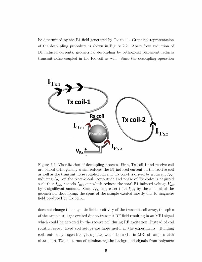
be determined by the B1 field generated by Tx coil-1. Graphical representation
of the decoupling procedure is shown in Figure 2.2. Apart from reduction of
B1 induced currents, geometrical decoupling by orthogonal placement reduces
transmit noise coupled in the Rx coil as well. Since the decoupling operation
Figure 2.2: Visualization of decoupling process. First, Tx coil-1 and receive coilare placed orthogonally which reduces the B1 induced current on the receive coilas well as the transmit noise coupled current. Tx coil-1 is driven by a current ITx1inducing IRx1 on the receive coil. Amplitude and phase of Tx coil-2 is adjustedsuch that IRx2 cancels IRx1 out which reduces the total B1 induced voltage VRxby a significant amount. Since ITx1 is greater than ITx2 by the amount of thegeometrical decoupling, the spins of the sample excited mostly due to magneticfield produced by Tx coil-1.
does not change the magnetic field sensitivity of the transmit coil array, the spins
of the sample still get excited due to transmit RF field resulting in an MRI signal
which could be detected by the receive coil during RF excitation. Instead of coil
rotation setup, fixed coil setups are more useful in the experiments. Building
coils onto a hydrogen-free glass plates would be useful in MRI of samples with
ultra short T2*, in terms of eliminating the background signals from polymers
9
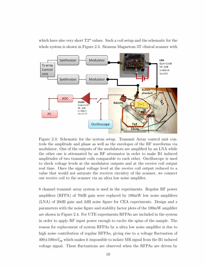
which have also very short T2* values. Such a coil setup and the schematic for the
whole system is shown in Figure 2.3. Siemens Magnetom 3T clinical scanner with
Figure 2.3: Schematic for the system setup. Transmit Array control unit con-trols the amplitude and phase as well as the envelopes of the RF waveforms viamodulator. One of the outputs of the modulators are amplified by an LNA whilethe other one is attenuated by an RF attenuator in order to make B1 inducedamplitudes of two transmit coils comparable to each other. Oscilloscope is usedto check voltage levels at the modulator outputs and at the receive coil outputreal time. Once the signal voltage level at the receive coil output reduced to avalue that would not saturate the receiver circuitry of the scanner, we connectour receive coil to the scanner via an ultra low noise amplifier.
8 channel transmit array system is used in the experiments. Regular RF power
amplifiers (RFPA) of 70dB gain were replaced by 100mW low noise amplifiers
(LNA) of 20dB gain and 2dB noise figure for CEA experiments. Design and s
parameters with the noise figure and stability factor plots of the 100mW amplifier
are shown in Figure 2.4. For UTE experiments RFPAs are included in the system
in order to apply RF input power enough to excite the spins of the sample. The
reason for replacement of system RFPAs by a ultra low noise amplifier is due to
high noise contribution of regular RFPAs, giving rise to a voltage fluctuation of
400±100mVpp which makes it impossible to isolate MR signal from the B1 induced
voltage signal. These fluctuations are observed when the RFPAs are driven by
10

zero input power. The resulting oscilloscope measurements are shown in Figure
2.5 for various zoom-in levels. In addition, there are time delays between the
transmit array channels due to software sychronization problems or some other
inherent nonlinearities of the synthesizers. An oscilloscope screen shot is shown
in Figure 2.6, displaying the signal induced in the receive coil after decouling
when two transmit coils are driven by modulator outputs via system RFPAs. //
Even with the use of an LNA at the output of the modulator transmit noise could
still affect the acquired signal out of a CEA experiment. It could be significant
to know the limits of the transmit noise for some applications. In case of analog
signal transmission, RF sources of very low noise, mixers and amplifiers with very
low noise could be helpful yet the existing noise would still be amplified by the
gain of the amplifiers in the transmit pathway. In Equation 2.3 total noise output
power is calculated [30] for the system shown in Figure 2.7.
Ni = kToB
No = F12G1G2Ni (2.3)
F12 = F1 +F2 − 1
G1
where Ni and No are input and output noise powers, respectively. k is the Boltz-
mann constant, To is the ambient temperature in Kelvin, and B is the system
bandwidth. Fn and Gn are noise figure and gain, respectively, of the component
n, and F12 is total noise figure of the system. It is shown in Equation 2.3 that
output noise is determined by the gain and noise figure of the system components,
thus it is significant to use low noise figure components and low noise sources in
the transmission circuits.
Another noise reduction technique would be to monitor the RF during excitation
by another receive channel and acquire the transmit signal alone in order to use
in signal processing as a reference line. In the experimental setup described in
this work, an LNA is included and also orthogonal placement of a transmit and
receive coil which is called geometrical decoupling help reduce transmit noise by
the amount of the geometrical decoupling.
For the first imaging experiments transmit coils were chosen as two channels of a
custom made 8 channel birdcage transmit coil of 35cm diameter with loop dimen-
sions of 8x16cm. Receive coil was a single loop coil of 6cm diameter tuned with
11

three distributed capacitors, matched to 50Ω, and the loaded quality factor is
measured as 130. Connections are made with 50Ω coaxial cables. The coil setup
is shown in Figure 2.8. This setup is later replaced by the glass coil setup as
shown in Figure 2.3. Following steps are to be followed to achieve the decoupling
task by decreasing the B1 induced voltage in the receive coil:
1. Using a rotation setup and transmitting RF from the transmit channel
amplified with the LNA, maximum amount of geometrical decoupling is
achieved by rotating the receive coil manually in angular direction while
measuring the B1 induced voltage with a digital oscilloscope (DSO6104A
Agilent). It is also possible to use a fixed coil setup where Rx coil and Tx
coil-1 are orthogonally placed and fixed at those positions.
2. Weaker RF was applied to the second transmit coil in order to remove the
remainder of the B1 induced voltage. B1 induced voltage at the receive
coil output is measured and recorded for single-channel and multi-channel
transmission cases. Amplitudes are adjusted such that both channel induces
the same amount of voltage in the receive coil. Using individual B1 induced
voltages V1 and V2, amplitude scale c is determined such as to set V1 and
cV2 equal. Using the B1 induced voltage measurement when both channels
transmit, relative phase value that makes total B1 induced voltage zero is
calculated by solving Equation 2.2 for θ.
3. Once the voltage induced on the receiver was reduced down the measure-
ment level of oscilloscope (2mVpp) the receive coil output is connected to
the scanner receive circuitry via a home made ULNA. Fine tuning of de-
coupling was proceeded by further adjustment of amplitude and phase of
transmit coils iteratively from the transmit array control CPU.
A special but common case about the decoupling is the time varying pulses.
The system response to the time varying frequency must be utilized in order to
determine the appropriate decoupling signal. For example, if the system has a fre-
quency response as shown in Figure 2.9b, the decoupling pulse can be calculated
with respect to the original transmit pulse and the systems frequency response
12

as shown in Figure 2.9d. Such an adjustment that allows for transmitting differ-
ent RF pulse shapes from different transmit coils would increase the decoupling
performance.
2.2 Application to UTE
The idea of using reduction of B1 induced currents in UTE sequences is first
presented in the literature [26] as a potential solution to the acquisition delay
problem in UTE sequences due to coil ring down time. For UTE sequence, ra-
dial inside out k space trajectory with 128 radial projections of a rubber sample
onto xy plane are acquired with RF pulse duration 100us and peak voltage 30V,
maximum gradient amplitude 24mT/m, and acquisition bandwidth 980Hz/pixel.
In radial inside-out k space trajectory, each spoke from center of the k space to
the end is the Fourier transform of the projection of the sample along the cor-
responding gradient direction. This approach is quite similar to the projection
reconstruction methods applied in CT, yet backprojection reconstruction algo-
rithms are not preferred in MRI since they are time consuming. Gridding the
projection data onto Cartesian coordinates, and then applying inverse Fourier
transformation is much more popular in MRI with non-Cartesian k space trajec-
tories [31]. Step by step description of the gridding process is stated below.
1. k space is covered in radial inside-out trajectory where each projection is
a single spoke from center to the outermost point of the k space. We first
define k space as a single vector and normalize the real and imaginary parts
of it to scale in [-0.5,0.5]. Normalized k space coordinates are assigned to
a vector named knorm which is the first parameter of the reconstruction
program and has a length of 128×128 in the first experiments and 256×768
in final experiments.
2. Raw data is averaged over all the averaging acquisitions (=10 in our experi-
ments) and arranged in a singe vector named rmean in the order of acquired
projections to match the knorm vector. rmean is the second parameter of
13

the reconstruction and has a length of 128× 128 or 256× 768 where there
are 128 or 256 data points for each projection spoke, respectively; and there
are 128 or 768 spokes, respectively covering a two dimensional circle.
3. Density correction function is calculated according to k space sampling
properties. Samples are located along radii at multiples of ∆kx =∆ky=∆kr.
The weighting to be applied during the gridding will be the inverse of the
sample density w(kx, ky) = 1/ρ(kx, ky). For Np radial projections, sample
at the center is acquired Np times. Therefore, the weighting for the samples
is 1Np
times the area of the central disk closest to the origin. Figure 2.10
shows the geometry used in calculation of the density correction function.
In Equation 2.4 formula for sample weightings is shown.
ωo =1
Np
π
(∆kr
2
)2
ω1 =1
Np
π
(3∆kr2
)2
−(
∆kr2
)2 (2.4)
ωn =2π
Np
(∆kr)2n
4. As calculated in Equation 2.4, density correction function for a projection
data set is simply a ρ filter.
5. Another parameter of the reconstruction funciton is cartesian grid matrix,
which is assigned a square matrix for ease of calculation. It is a 128× 128
or 256× 256 matrix for our case.
6. Finally, we define the interpolation kernel to be used in gridding task which
assigns each cartesian grid point to its value determined by convolution of
the interpolation function with nonuniformly sampled data. Keiser-Bessel
function is used as the interpolation kernel as shown in Equation 2.5.
kerneltable =1
W
[β√
1− (2u/W )2]
(2.5)
The function is defined over |u| < W/2, with parameters W being kernel
width and β as a free design parameter.
14

7. Once we form all the parameters, we calculate the gridded data points
by running the grid(rmean,knorm,dcf,gridmatrix,kerneltable) function we
developed using MATLAB R© (version 7.10.0, Mathworks Inc., Natick, MA).
This function calculates the value of each grid point based on the result
of the convolution of the raw data with the gridding kernel. Raw data is
multiplied by the density correction function.
8. Output of this funciton is inverse Fourier transformed and the image is
formed. In Figure 2.11 gridding operation is schematically presented.
Pulse sequence diagram is shown in Figure 2.12. In the first experiments ac-
quired raw data is mapped onto a Cartesian grid of size 128x128 for using a zero
order gridding algorithm which assigns the average value of 8 closest samples in
nonuniformly sampled k space data to a point on the Cartesian grid. Inverse 2D
Fourier transformation is applied afterwards. Increasing the number of projec-
tions would help increasing the field of view and eliminating aliasing artifacts of
high frequncy components. In order to obtain images with better signal to noise
ratio, peak RF voltage should be increased. Gridding operation can also be im-
proved by applying higher order interpolations such as Keiser-Bessel interpolation
before assigning the values for cartesian grid points as stated previously. Blurring
due to fast T2* decay in the acquired raw data should be corrected before grid-
ding operation. The basic signal formulation derived for regular MRI sequences
does not account for T2* decay. However, if we include this effect in the formula-
tion [32], it is obvious that we need to deconvolve the acquired projections with
reciprocal of an exponential decay determined by T2* of the sample as shown in
Equation 2.6. However, multiplication of FID with T2* decay correction function
results in noise amplification at high frequency regions of the k space. Such a
noise enhancement can be eliminated with an apodization correction. The effect
of an apodization will be observed as a gain in signal to noise ratio compared
to the case with only T2* decay correction applied. These corrections can be
combined in a single function with an additional constant value that prevents
loss of the low frequency information. The resulting correction function is shown
15

in Figure 2.13.
s(t) =∫m(x)e−j2πkx(t)xe−t/T
∗2 dx
kx(t) = γ∫ t
0Gx(t
′)dt′ (2.6)
s(t)et/T∗2 =
∫m(x)e−j2πkx(t)xdx = M(kx)
where s(t) is the complex FID signal in rotating frame, Gx is the gradient along
x direction, m(x) is the spin density distribution along x direction, and M(kx)
is the Fourier transform of the spin density distribution which is T2* corrected
FID signal. As an alternative to such a correction function with sharp transi-
tions, a function having more smooth transitions can be more useful for certain
applications. One such example is given in Equation 2.7.
f(t) = et− t
an
T∗2 (2.7)
where a and n are free design parameters describing sharpness and cut-off of the
filter depending on T2* decay. Advantages of such parametric funcitons include
being suitable to be used in optimization programs and eliminating artifacts due
to sharper transitions in frequency domain.
In case of imaging of a sample that is a mixture of long and short T2* values, it is
possible to excite only the spins with short T2* value by off-resonant excitation.
Since the spins of short T2* value have broader resonance bandwidth, excitation
bandwidth can be shifted such that spins with long T2* value are not excited.
Note that off resonance shift must account for the existence of spatial encoding
gradients as well.
2.3 Application to CEA
The expected signal for a concurrent excitation and acquisition experiment with
rectangular RF is simulated in MATLAB R© as the magnitude of the transversal
magnetization vector during excitation [33]. Bloch equation is solved numerically
using rotation matrices and the transverse magnetization is calculated under the
small-tip angle approximation [34] as shown in Figure 2.14. Simulation results
16

show that a decaying oscillation should be observed out of a CEA experiment,
where the decay and oscillation characteristics determined by B1 field magnitude
and relaxation parameters of the sample . Time constant of the decay is deter-
mined by the T2* value of the sample. Peak amplitude of the decaying oscillation
depends on the B1 field magnitude. The magnetic field strength will determine
the received signal magnitude. Note that in the simulation, noise sources and
any other influences of experimental complications such as imperfections in de-
coupling are ignored.
In NMR theory spins are described as linear systems with the impulse response
being the free induction decay (FID) behavior of the spins under relaxation. A
CWNMR experiment is modeled as a linear system operation where the input
is B1 excitation signal and the output is the convolution of the system response
(FID) and the input B1 which is a chirp signal covering a certain frequency
range [35]. Detailed formulation is also given in literature [8] for short T2*
and small tip angle approximation in order to account for linearity condition of
spins during CW excitation. Acquired raw data in a CEA experiment can be
formulated as additive combination of such a convolution signal and a frequency
dependent leakage component which is the remaining B1 induced voltage due to
limited decoupling as shown in Equation 2.8.
s(t) = FID ⊗B1(t) + A(t)
s(t) = FID ⊗B1(t) + h(t)⊗B1(t) (2.8)
B1(t) = e−jπfs/tacqt2
In Equation 2.8, A(t) is the frequency/time dependent leakage signal due to insuf-
ficient decoupling. We can model this leakage by an experimentally determined
system response h(t), which is the time dependent response of the data acquisi-
tion system against the B1 induced voltage. Since the frequency is swept linearly
through time, the leakage response can also be treated in frequency domain which
is an intrinsic property of the chirp signal. h(t) can be measured separately in a
CWNMR experiment provided that no MR signal exists in the acquired signal.
The ratio of frequency sweep range fs and the total RF duration tacq is regarded as
the frequency sweep rate. In literature [36], the leakage signal for hybrid coupler
systems used in classical CWNMR systems with lock-in detection is formulated
17

as in Equation 2.9.
A(w) =Rcoil
1 + ∆w2τ 2+ j
Rcoil∆wτ
1 + ∆w2τ 2(2.9)
It is reported in [24] that a second order fitting is sufficient to approximate A(w)
(We use A(t) analogically to A(w) due to linear sweep of frequency over time)
instead of solving equation 2.9 analytically. Another method is to measure the
received signal when the receive coil is unloaded [37]. In the CEA experiments,
two subsequent data are acquired, one with the regular experiment setup and the
other with the sample is removed. The difference of two cases is considered to
be the raw MR signal that is to be deconvolved with B1 to get FID response.
The measurement data when the sample is removed is used as B1 signal. Note
that the amplitude of the B1 induced leakage signal may differ for subsequent
measurements due to instabilities occurring in Tx-Array control unit. Therefore,
we take averages of repetitive measurements to account for a better fitting.
It should be noted that position dependence of B1 is ignored in Equation 2.8. B1
inhomogeneities were not taken into account during experiments, as well. In fu-
ture studies, in order to make position dependence of B1 ineffective, adiabaticity
of the applied B1 waveform should be increased since adiabatic pulses rotate the
magnetization vector at constant flip angle, even when B1 is extremely inhomo-
geneous [38].
We drive Tx coil-1 from a Tx array modulator output via an LNA, while Tx coil-2
is driven directly from the modulator output without amplification. Orthogonal
placement of Tx coil-1 and Rx coil is significant to reduce transmit noise coupled
on the receive coil in CEA applications. Decoupling is done by adjusting ampli-
tude scales and relative phases of Tx coil-1 and Tx coil-2 so that individual B1
induced currents on the Rx coil cancel each other. Tx coil-1 is driven with RF
input power of 8mW and Tx coil-2 with 0.4mW. After the decoupling is achieved,
B1 induced voltage is reduced to 0.5mV including the preamplifier gain of 35dB
with 0.8dB noise figure. First experiments are conducted with a rectangular re-
ceive loop coil loaded with a plastic bottle of 7cm diameter and 15cm height full
of tap water solution of 1gr/l saline and 1gr/l CuSO4 (εr=60, σ=0.2 S/m). See
Apendix A for measurement of dielectric constant and conductivity values. For
the recent imaging experiments a glass coil setup is used instead of the plastic
18

one in order to prevent background signals formed by ultra short T2* substances.
Liquid samples used for loading of small loop coil are put in a cylindrical glass cup
with 6cm diameter and 5cm height. 50% ethanol and water solution is the liquid
sample used for spectroscopy experiment. Chirp pulses with certain frequency
sweep range and pulse durations are calculated in MATLAB R© and inserted in
pulse sequence executive files using pulse programming environment IDEA of
Siemens Medical Systems. Zero gradient case and gradients corresponding to ra-
dial k space trajectory are also programmed using IDEA as shown in the pulse
sequence diagram of a single TR duration in Figure 2.15. Raw data is read and
saved with a MATLAB R© program and average of 10 acquisitions for each case is
assigned to vector variables. Reconstruction formula is inserted in a MATLAB R©
function and 1-D projections are calculated along each gradient direction as well
as the spectrum of the sample.
|B1| value is also calculated using Bloch-Siegert shift method in order to estimate
the flip angle. In B1 mapping with Bloch-Siegert shift method, an off resonant
RF is applied which results in spins to experience an additional phase shift. Using
the fact that the additional phase is proportional to |B1|2 it is possible to get
B1 map from the phase images [39]. B1 maps are generated for reference input
voltage level of 20V with a Fermi pulse of 8ms duration and 4kHz off resonance
from the center frequency using the Equation 2.10 after unwrapped phase maps
are obtained [40]. This reference value is used to approximate the flip angle and
B1 values achieved in CEA experiment by assuming that the flip angle and B1
value are linearly dependent on the input voltage level and the RF duration.
φ ≈∫ T
0
|γB1(t)|2
2ωOFF (t)dt. (2.10)
where φ is the phase value and ωOFF is the off resonance of the RF pulse from the
center frequency. Note that this equation for |B1| is an approximation and can
be corrected with a modification that includes higher order terms [41]. However,
for the small flip angle values as in our case, it should be a valid approximation
to use Equation ??
Chirp RF pulse of 0.5V with 4.2ms duration and 4.2kHz sweep range is applied
and acquisition is started 100µs after RF starts. Reconstruction of CEA data
starts with subtracting the remaining RF leakage induced in the receive coil from
19

the acquired raw data. Deconvolution of the raw MR signal with the measured
B1 field is done afterwards for each projection line. The rest is the same gridding
approach as in the UTE reconstruction. It should be noted that no filters or any
other signal processing is applied to the raw data except the RF leakage subtrac-
tion, deconvolution, and the zero-order gridding operations unless specified.
20

(a) Circuit diagram of the LNA
(b) S parameters, Noise figure and Stability Factor
Figure 2.4: Circuit diagram and s parameters with noise figure and stability factorof the amplifier used in the experiments. Single stage amplifier is built with aBFG135 bipolar transistor with input and output matchings are performed.
21

Figure 2.5: Distortions on the output waveforms of the original 4kW system RFpower amplifiers measured with oscilloscope. System RFPAs are driven by inputRF signal amplitude of which is set to zero from MR console. Nonlinear effectsof the amplifiers are observed as 400mVpp fluctuation signals.
22

Figure 2.6: The peaks are observed at the end of signal envelope due to a delayabout 10µs between transmit channels. This effect is eliminated in the CEAexperiments by starting acquisition 100µs later than RF starts.
Figure 2.7: System with a thermal noise source, and two active components.
Figure 2.8: Experimental setup with a 8 channel birdcage transmit and a receiveloop coil. A rubber phantom is placed on the receive coil.
23

Figure 2.9: Demonstration of decoupling when B1 induced voltage signal has atime dependence. Transmit sinc pulse with a single side lobe (a). Spectrum ofthe sinc pulse (b). Frequency response of the decoupling system in 1024Hz range(c). Required transmit pulse for better decoupling than decoupling using thesame pulse transmitted from both sources (d).
Figure 2.10: Calculation of the sampling density for a projection raw data set.
24

Figure 2.11: Nonuniformly sampled data is transformed into Cartesian gridpoints. Value of a grid point is assigned by interpolation.
(a) UTE pulse sequence diagram for radial k space trajectory
(b) Pulse sequence diagram for a single TR
Figure 2.12: Pulse sequence diagram for CEA with 128 radial projections and asingle time of repetition (TR) interval.
25
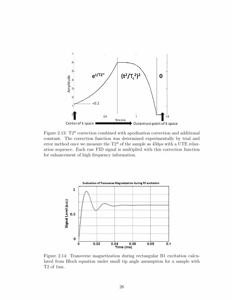
Figure 2.13: T2* correction combined with apodization correction and additionalconstant. The correction function was determined experimentally by trial anderror method once we measure the T2* of the sample as 450µs with a UTE relax-ation sequence. Each raw FID signal is multiplied with this correction functionfor enhancement of high frequency information.
Figure 2.14: Transverse magnetization during rectangular B1 excitation calcu-lated from Bloch equation under small tip angle assumption for a sample withT2 of 1ms.
26

Figure 2.15: Sample pulse sequence diagram representing excitation, acquisitionand encoding timings and magnitudes for a single TR interval. Gradients alongwith the sweep range determine the FOV and resolution. Changing the orienta-tion of the gradients means acquiring projections along various directions.
27

Chapter 3
Results
3.1 Decouping of RF Coils
We achieved decoupling of 70dB which corresponds to total of 20dB geometrical
decoupling and 50dB multiport decoupling. In the beginning, the receive coil
loaded by a sample of copper sulfate solution is attached to the rotation setup
and placed in the scanner. Then, coil plane is rotated counter clockwise with
a step size of 5o. The voltage induced in the receiver coil, which is measured
80 ± 5mVpp at its maximum, is recorded by the oscilloscope. The rotation step
size is reduced to 0.5o when needed in order to observe the induced voltage to be
decreased. Resulting plot for geometric decoupling simulation and experimental
data are shown in Figure 3.1. Geometric decoupling is done for one RF generator
unit connected to one of the channels of the birdcage coil with an LNA of 20dB
gain and 2dB noise figure connected at the modulator output. Then, the other
channel of the modulator output of the RF generator unit is connected directly
to another channel of the birdcage coil with an attenuator enough to adjust indi-
vidual B1 induced voltages close to each other, in this case 6dB attenuator was
used with the initial setup. For the glass coil setup, tuning of the Tx coi-2l is
shifted from on resonant in order to reduce the coupling instead of using atten-
uators. Once a second RF generator unit is connected to the second transmit
28

Figure 3.1: B1 induced voltage is measured for rotation of the receive coil planewith respect to one of the transmit coils covering 180o. Ideal linearly polarizedfield is calculated and both normalized to 0o to impress the effect of getting closerto ideal condition. The limitation in this task is that individual polarizations ofthe transmit coils are slightly elliptically polarized. One should also considerphysical dimension of the coils and the distance between them because receivecoil can affect the loading of transmit coil when they are placed too close to eachother and their physical dimensions are similar, due to strong mutual coupling.
coil, we record the voltages induced by single channel transmissions and multi-
channel transmission. Using the recorded data, the phase value that minimizes
total B1 induced current is calculated. Observing the induced voltage, phase of
one of the RF generator units is adjusted within possible precision via transmit
array control unit. Initial voltage of 8 ± 1mVpp that corresponds to the voltage
induced after the geometrical decoupling is reduced further to 6 ± 4µVpp with
multiport decoupling after phase adjustment. Induced voltage is recorded for a
range of relative phase values of the RF generator units with step size of 10o.
Step size is reduced when required. The resulting plot for achieved decoupling is
shown in Figure 3.2. Orthogonal placement of transmit and receive coils helps
reduce transmit noise induced voltage signal as well as the B1 induced voltage.
We expected that the transmit noise induced voltage would be a dominant factor
in the acquired signal. However, we observed that acquired signal voltage levels
were the same for two cases: when the transmit system is driven by zero input
29

Figure 3.2: Decoupling versus Phase of an RF generator unit. Two-port decou-pling is represented by changing the phase of one port in uniform steps covering360o. Data are normalized to 0o. Limitations of decoupling using this procedurearises from the precision of the phase control unit. Stability of the RF generatorunit is also a key factor for the achieved decoupling to be preserved during theexperiment. Addition of a third coil could increase the amount of total decouplingwhich could be used to cancel remaining B1 current on the receive coil.
power; when the transmit system is turned off. Therefore we concluded that
the transmit noise induced voltage is lower than the receive noise floor, whereas
calculation of transmit noise could be needed for extreme conditions with higher
transmit noise. The effect of geometrical decoupling on reduction of transmit
noise is demonstrated in Figure 3.3 where B1 induced signals are shown from an
experiment with multiport decoupling applied alone, and various levels of geomet-
ric decoupling applied with multiport decoupling. It is shown that increasing the
amount of geometrical decoupling, noise fluctuations in the receive coil decreases.
The problem with multiport decoupling is that when the transmit fields are of
different sources, they have different noise characteristics and it is not possible
to decouple noise with B1 induced current cancellation technique when the noise
has uncorrelated sources. However, orthogonal placement simply eliminates the
B1 induced current by all means whether it is noise or the signal itself. // An-
other experiment is conducted to demonstrate the feasibility of decoupling with
30

Figure 3.3: B1 induced voltage signal in the receive coil after decoupling. Mul-tiport decoupling without geometric decoupling (a), Multiport decoupling with10dB geometric decoupling (b), Multiport decoupling with 20dB geometric de-coupling (c).
transmit RF pulses of different shapes. One such example is shown in Figure 3.4
where the system frequency response is used to obtain optimum RF waveform to
be transmitted from second transmit channel for better decoupling. The result-
ing B1 induced voltage signals after decoupling are compared for the same RF
and different RF waveorm cases in Figure 3.5. It is observed that, estimating
the RF waveform to be transmitted from the decoupling coil based on the sys-
tem response reduces the deviation of leakage level with respect to the frequency.
The amount of achieved decoupling is also increased when two transmit coils are
driven by different RF waveforms. However, the system stability prevented us
from using this approach in imaging experiments. The system response shows
31

variability among the experiments and also it is time consuming to update the
estimated RF waveform each time. Therefore, in this study we only show the
feasibility of this approach in decoupling procedure which could be improved and
further utilized when system stability problems are resolved by designing more
reliable system components.
Figure 3.4: B1 induced voltage signals in the receive coil for single channel trans-mission with varying input levels by changing the amplitude scale of a chirp RFsignal spanning -8kHz to 8kHz over 8ms from Tx array user interface (a). Esti-mated system response for actual input level (b). Estimated RF waveform to betransmitted from the decoupling coil i.e. Tx coil-2 (c).
32

Figure 3.5: B1 induced voltage signal in the receive coil after decoupling with thesame RF waveform transmitted from both transmit channels (a), and a differentRF waveform transmitted from the decoupling coil as shown in Figure 3.4c (b).
3.2 Application to UTE
2D image for UTE is shown in Figure 3.6. There are artifacts based on the
projection reconstruction method employed here is not being so powerful. Center
of k space is missed in the UTE data which result in center brightening artifact.
However, the dots and the edges as high frequency information are represented
in the image clearly. It is expected that the time delay between the RF turn off
and acquisition start would be decreased with increasing amount of decoupling
yet this could not be demonstrated in the imaging experiments because we had
to include RFPAs in our setup. RFPAs induce high levels of fluctuation signal
due to blanking of the RFPAs before transmission starts and this prevents us
from decreasing the acquisition delay further than 20µs. In fact, a time delay
of 10µs between the transmit channels which resulted in spikes at the end of
the RF pulse is observed and we had to put a 20µs time delay at the end of
the RF before starting the acquisition in UTE sequence. Increasing the input
RF peak voltage to 240V and the number of k space lines to 768, we observe
33

Figure 3.6: Rubber phantom with holes (a). UTE image for 128 projections and30V peak RF input voltage (b).
in Figure 3.8a that the signal level increases, yet there are still artifacts in
the image. Another improvement is the use of Kesier-Bessel interpolation and
sampling density correction for gridding operation. Sampling density correction
matrix is formed by calculating the sampling density along the angular direction
from inside out. The samples become less dense when we move away from center.
For the k space trajectory used for 768 lines with max gradient level of 14mT/m
the density correction over each projection is included in the gridding process.
T2* correction is also applied to the acquired data which enhances the edges of
the image of the rubber as shown in Figure 3.8b. The effects of T2* correction on
the FID signal and a single projection are shown in Figure 3.7. In Figure 3.9 the
effect of acquisition delay on the image quality is demonstrated as well. Increasing
the time between excitation and acquisition we start to lose information which
becomes even more obvious for samples with short coherence time. We observe
that image quality increases with increased number of projections. The effect
of T2* correction is observed as sharpness in the projections which explains the
reason for edge enhancement of the image. There are some other artifacts in
the image that should be eliminated before advancing to a clinical application of
these sequences.
34

Figure 3.7: Demonstration of the T2* correction effects on the UTE signal of arubber sample: FID (a) and projection (b) enhancement using T2* correction asdefined in Chapter 2.
3.3 Application to CEA
B1 map for 20V reference input is shown in Figure 3.10. Using the average B1
value of this experiment we can estimate the achieved flip angle with linearity
approximation between input transmit voltage and the B1 value. For a rectangu-
lar RF with 1V amplitude and 8ms duration, the resulting flip angle is estimated
as 6o. Note that the B1 map is generated for only the transmit channel with the
higher input voltage i.e. Tx coil-1. Therefore, we must expect the magnetization
to be deviated from its intended orientation depending on the RF transmitted
from the second transmit channel with a lower input voltage. However, the
amount of this deviation must be smaller than 10% since there is a 20dB differ-
ence between the input voltages of the transmit channels. Concurrent MRI signal
is obtained by using a transmit array system to achieve the decoupling task. In
the first experiments transmit coils are driven by on resonant RF waveform with
rectangular envelope and 0.8mW RF input power is transmitted. In Figure 3.11,
the raw data is acquired with all the gradients are turned off, meaning that signal
is acquired from the whole sample. Turning on the slice selection gradient in the
data acquisition chain, the MRI signal decreases in magnitude as shown in Fig-
ure 3.12. These results showing that we are able to detect MR signal during RF
excitation are presented in [25,27,28]. The fluctuation voltage level observed at
35

Figure 3.8: UTE image of a rubber sample for 768 projections, 240V peak RFinput voltage and acquisition delay of 20µs without (a) and with T2* correction(b).
the receive coil is reduced to 30µV with the aid of geometrical decoupling. Delay
of 10µs is observed between RF generator units which results in degradation of
decoupling at the beginning and at the end of the RF envelope. Therefore, data
acquisition is started 100µs after the RF is turned on. B1 value is estimated as
0.2µT using Bloch-Siegert shift method assuming B1 is proportional to the input
RF peak to peak voltage level.
In order to increase the signal level we have inserted a 100mW LNA of 20dB gain
and 2dB noise figure after the modulator output of one of the transmit channels.
Figure 3.13 corresponds to the raw data for the case that small circular loop is
loaded with tap water and CEA experiment is conducted for ±500Hz sweep over
40ms. We observe that when the RF passes through spins are excited and they
lock into the B1 field and precess around the effective B1 as in an adiabatic slow
passage experiment . For visualization of the deconvolution process Figure 3.14
shows the acquired raw data processed through leakage subtraction, a smoothing
filter, and deconvolution. Deconvolution results in the FID signal in rotating
frame which can be transformed either into a projection if any gradients exist
during excitation or frequency spectrum containing chemical shift resonance and
scalar coupling information. Figure 3.15 shows the spectrum for ethyl alcohol
36

Figure 3.9: UTE image for 768 projections, 240V peak RF input voltage andacquisition delay of 20µs (a), 80µs (b), 120µs (c) and 200µs (d) .
and water solution produced for -1kHz sweep over 40ms. The acquired raw sig-
nal is difficult to interpret, yet applying deconvolution and low pass filters we
could observe the chemical shift spectrum of separated hydrogen components of
ethanol. This spectoscopy result is first presented in [26, 29]. 2D images for
CEA sequence are shown in Figure 3.16. K space trajectories and the gridding
algorithm is the same as the UTE image shown in Figure 3.6. We can observe
the epoxy plate on which the Rx coil is built. Different from UTE image, here
the center of k-space is not missed since the spins are not dephasing during RF
excitation. Therefore, we observe a smoother image and the holes are distinc-
tive, but the edges are lost.It should be noted that no filters or any other linear
37
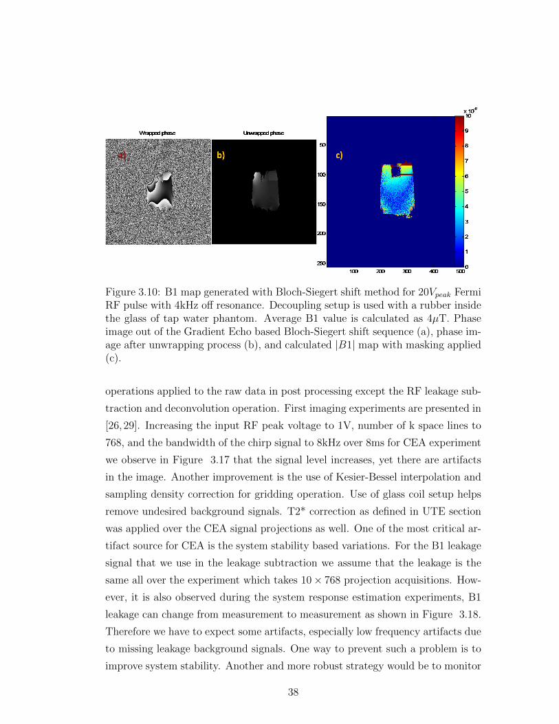
Figure 3.10: B1 map generated with Bloch-Siegert shift method for 20Vpeak FermiRF pulse with 4kHz off resonance. Decoupling setup is used with a rubber insidethe glass of tap water phantom. Average B1 value is calculated as 4µT. Phaseimage out of the Gradient Echo based Bloch-Siegert shift sequence (a), phase im-age after unwrapping process (b), and calculated |B1| map with masking applied(c).
operations applied to the raw data in post processing except the RF leakage sub-
traction and deconvolution operation. First imaging experiments are presented in
[26, 29]. Increasing the input RF peak voltage to 1V, number of k space lines to
768, and the bandwidth of the chirp signal to 8kHz over 8ms for CEA experiment
we observe in Figure 3.17 that the signal level increases, yet there are artifacts
in the image. Another improvement is the use of Kesier-Bessel interpolation and
sampling density correction for gridding operation. Use of glass coil setup helps
remove undesired background signals. T2* correction as defined in UTE section
was applied over the CEA signal projections as well. One of the most critical ar-
tifact source for CEA is the system stability based variations. For the B1 leakage
signal that we use in the leakage subtraction we assume that the leakage is the
same all over the experiment which takes 10× 768 projection acquisitions. How-
ever, it is also observed during the system response estimation experiments, B1
leakage can change from measurement to measurement as shown in Figure 3.18.
Therefore we have to expect some artifacts, especially low frequency artifacts due
to missing leakage background signals. One way to prevent such a problem is to
improve system stability. Another and more robust strategy would be to monitor
38

Figure 3.11: Concurrent MR signal acquired using 3T transmit array system withTR=1000 ms, Resolution =512, Acquisition BW: 50Hz/Px. This data is unpro-cessed raw data including B1 induced voltage signal remaining after decoupling.If leakage is higher the oscillations due to magnetization induced signal would beinvisible. Since there is no gradient applied, the signal is accumulated all overthe sample volume.
the RF waveform real time thorughout the experiment and use the monitored RF
signal in all of the calculations that use B1 field. There is much to do for signal
processing part, yet the purpose of this study is to demonstrate the feasibility
of MRI with CEA and UTE techniques with the method of decoupling we have
developed.
39

Figure 3.12: Concurrent MR signal acquired with 20mT/m slice selection gradientturned on at t=4ms. Turn on of gradient causes the signal level to drop imme-diately. The space encoded information can be extracted with weaker gradientsand higher B1 applied. In this experiment, the input RF power was 0.8mW
Figure 3.13: Raw data out of a CEA experiment for chirp B1 excitation of±500Hzover 40ms observed in water phantom.
40

Figure 3.14: Acquired raw data from a water sample (a). Input B1 waveform asa chirp function (b). Acquired signal after the leakage subtraction (c). Fouriertransform of the estimated FID signal after deconvolution (d) and single-sidedFID signal which is an approximation of the actual FID (e).
41

Figure 3.15: Raw data acquired from ethanol sample (a). Chemical shift spectrumobtained after deconvolution (b).
Figure 3.16: Rubber phantom of T2 of 500µs with holes (a). CEA image (b).
Figure 3.17: Rubber phantom of T2 of 500µs with holes (a). CEA image withimproved imaging parameters and gridding with Keiser-Bessel interpolation (b),and T2* correction applied (c).
42
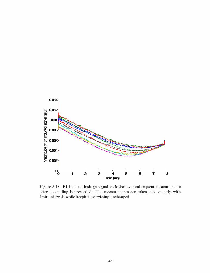
Figure 3.18: B1 induced leakage signal variation over subsequent measurementsafter decoupling is preceeded. The measurements are taken subsequently with1min intervals while keeping everything unchanged.
43

Chapter 4
Discussions
Decoupling performance depends strictly on the sensitiveness of the rotation setup
and the degree of precision of the RF generator phase adjustment unit. Transmit
noise has become a significant factor in our system. In the experiments we ex-
cluded RF power amplifiers from the setup because the amplifiers add noise during
transmission. Our aim is to implement spectroscopy and imaging of samples with
ultra-short T2* using CEA without being limited to gapped pulse sequences or
frequency sweep approaches. Using the method presented in this study both RF
excitation and signal acquisition can be set on resonant. This method provides
wide range flexibility for the applied RF field. As long as multiple transmit ele-
ments with controllable phase and amplitude are used, magnetic field decoupling
can be achieved. Dynamic range requirement is also lower compared to other
isolation methods.
Use of more than two transmit coils would help further reduction of remaining B1
induced voltage after multiport decoupling. However, coupling between transmit
coils should also be considered carefully before such an advancement. Decoupling
with two transmit coils is proceeded with experimental methods. However, some
preliminary studies using numerical simulations or approximate analytical solu-
tions that would help us to understand decoupling problem including more than
two transmit coil elements.
The methods for isolation between the MR signal and the B1 induced voltage
44
signal suffer from being too much motion sensitive, in general. Object motion
during acquisition does not only cause motion artifacts but also the decoupling
performance changes due to the changes in coil impedance. Therefore, the ob-
ject motion should be minimized in CEA applications. Object motion can be
observed as changes in coil impedances. Variation of coil impedances results in
variations of B1 induced voltage between subsequent acquisitions. Therefore,
real-time recording of excitation RF field is necessary for an automatic recon-
struction process suitable to pre-clinical and clinical applications.
The current system is to be optimized and modified to make its use convenient in
research and for clinical purposes. For in vitro measurements and spectroscopy
studies, a motor controlled rotation mechanism receiving a feedback about the
magnetic fields can be used. However, for clinical use and in vivo measurements,
it is not feasible to rotate patients and therefore the system design must be mod-
ified appropriately. For that purpose, transmit coils can be rotated around the
patient. More feasible transmit coil design would be using a transmit array of N
channels where N small coils are driven by embedded RF generator units which
can be FPGA controlled. Geometrical decoupling could be achieved by selection
of appropriate coil sets and multiport decoupling can easily be achieved using the
remaining elements of the transmit coil array. This design has advantages over
others for not having a moving part inside the scanner. Besides, small transmit
coils upgrades linearity of the transmit field and the multiport decoupling in-
creases the amount of decoupling compared to decoupling with two transmitting
coils.
The effect of transmit coil with weaker B1 field on the MRI signal can be ob-
served as a residual in the magnitude of the magnetization. We did not include
this effect in our analysis assuming that it is a minor effect. However, the effect
of multiple coil transmission on the magnetization vector must be analyzed in
detail for a more rigorous treatment of the acquired signal.
Gradients forming the radial k-space trajectory can be designed such that instead
of switching gradients on and off to acquire projections along different radial di-
rections, by changing gradient levels only, the same projections could be acquired.
If the gradient level is changed immediately after one projection is acquired and
kept on for a certain time interval until the next acquisition starts, spins that
45
are excited will be spoiled and the effect of the previous excitation will not last
during the next excitation. This continuous gradient approach can be applied to
2D and 3D imaging with k space trajectories that do not necessitate switching
the gradients on and off. Such a gradient design would eliminate the acoustic
noise in MRI scans significantly.
Other than thermal noise, there may be some other interference causing distor-
tions in the transmitted RF signal that we are not able to point out explicitely.
Some of the distortion sources might be voltage fluctuations, modulator based
frequency shifts, phase noises based on oscillator infidelities, and cable interfer-
ences. Such distortions and noise are hard to deal with when they are emitted
from independent sources. Different RF sources have different noise characteris-
tics implying that although we reduce the induced voltage through decoupling,
we may not be able to reduce the noise, but increase the noise. As a result, the
system introduced in this work is hard to implement using standard MRI systems
and needs particular design considerations addressing all these challenges. Use of
a single RF generator unit with a power splitter is a useful approach that cancels
RF generator unit based abnormalities. For example, field of two transmit coils
fed up by one RF generator unit with a power splitter will cancel the abnor-
malities as well as magnetic fields coupled in the receiver coil because identical
abnormalities are delivered to both coils. Such a system would allow to work
with higher RF input powers with our system being more tolerated to the noise
introduced by the transmit sources.
We have demonstrated the UTE and CEA sequences using a transmit array sys-
tem and the decoupling over 70dB is achieved which eliminates the need for a
detuning diode in the receive coil. Subtraction of MRI signal and B1 induced
voltage is still required for image reconstruction of CEA. Advantages of CEA
sequence are that it has much lower peak power and true zero echo time. Use of
very low RF input powers could also be significant for some applications. The
isolation method presented in this work is a potential solution to receiver dynamic
range problems in implementation of CEA. Further isolation between MR signal
and RF is achieved compared to other methods.
Improving the decoupling, signal level in CEA experiments will be increased sig-
nificantly. The system introduced in this work stands for a promising system
46

for implementation of NMR applications such UTE, CWNMR; and a powerful
alternative for recently proposed CEA methods such as sideband excitation and
continuous SWIFT.
Time interleaved approach in MRI results in limitations in echo time due to gradi-
ent and RF coil switching times, coil ring down times and acquisition bandwidth.
The idea of concurrent excitation and acquisition overcomes these problems due
to its intrinsic property of zero echo time. CEA using magnetic field decoupling
with transmit array enables the detection of on resonant MRI signal during on
resonant excitation. Therefore, there will be no need for RF coils to be turned
off but the receiver unit can acquire signal at any time point and acquisition
bandwidth is not limited. In addition, CEA provides us with the knowledge of
spin properties during excitation. Since excitation lasts much shorter than the
relaxation, imaging using spin parameters identifying excitation characteristics
will take shorter in time.
47
Chapter 5
Conclusions
In this study, a new method for decoupling of coils is introduced and the use of this
method in concurrent radio frequency (RF) excitation and MRI signal reception
is demonstrated. This study shows that RF signal coupled in the receive coils can
be reduced by more than 70dB using a transmit array system of two transmit
elements. MR signal can be detected directly independent from the shape of
RF. Subtraction of MRI signal and the B1 induced voltage is still required for
image reconstruction. Preliminary results indicate that this isolation method
is potentially useful in MRI and spectroscopy applications requiring concurrent
excitation and acquisition (CEA) and/or zero echo time as well as it can be used
as an additional decoupling procedure to the existing decoupling methods. The
isolation method presented in this work is a potential solution to the receiver
dynamic range problems in implementation of CEA. Further reduction of on
resonant B1 induced voltage is achieved compared to that is achieved using other
methods. It is also demonstrated that the acquisition delay in ultra short echo
time (UTE) techniques can be reduced using this method of decoupling.
Significance of CEA reveals itself in the limits where UTE methods are insufficient
such as solids and tightly bounded water in bones. Currently, MRI field is seeking
for the best short T2* imaging method. There are many short T2* imaging
methods suggested such as UTE [5], ZTE [15], SWIFT [12], WASPI [42], SPI [43]
and so on. CEA is supposed to be an alternative to these despite its challenges
48

in implementation some which are stated in this thesis and few are resolved.
The decoupling method we have developed is not restricted to use in CEA or the
potential use in UTE. It presents a novel approach to get benefit from transmit
array opportunity in MRI where we have transmit set of coils, decoupling set
of coils and receive coils. This method can find other applications where B1
induced currents are needed to be decreased without changing the sensitivity of
the transmit field.
49

Bibliography
[1] P. Gatehouse and G. Bydder, “Magnetic resonance imaging of short T2 com-
ponents in tissue,” Clinical radiology, vol. 58, no. 1, pp. 1–19, 2003.
[2] M. A. Schmidt, G.-Z. Yang, P. D. Gatehouse, and D. N. Firmin, “FID-based
lung mri at 0.5 T: Theoretical considerations and practical implications,”
Magnetic resonance in medicine, vol. 39, no. 4, pp. 666–672, 1998.
[3] D. J. Tyler, M. D. Robson, R. M. Henkelman, I. R. Young, and G. M. Bydder,
“Magnetic resonance imaging with ultrashort TE (UTE) pulse sequences:
technical considerations,” Journal of Magnetic Resonance Imaging, vol. 25,
no. 2, pp. 279–289, 2007.
[4] D. Lurie, S. McCallum, J. Hutchison, and M. Alecci, “Continuous-wave NMR
imaging of solids.,” MAGMA, vol. 4, no. 1, pp. 77–81, 1996.
[5] M. D. Robson, P. D. Gatehouse, M. Bydder, and G. M. Bydder, “Magnetic
resonance: an introduction to ultrashort TE (UTE) imaging,” Journal of
computer assisted tomography, vol. 27, no. 6, p. 825, 2003.
[6] P. C. Lauterbur et al., “Image formation by induced local interactions: ex-
amples employing nuclear magnetic resonance,” Nature, vol. 242, no. 5394,
pp. 190–191, 1973.
[7] R. R. Ernst, G. Bodenhausen, A. Wokaun, et al., Principles of nuclear mag-
netic resonance in one and two dimensions, vol. 14. Clarendon Press Oxford,
1987.
50

[8] R. K. Gupta, J. A. Ferretti, and E. D. Becker, “Rapid scan Fourier transform
NMR spectroscopy,” Journal of Magnetic Resonance (1969), vol. 13, no. 3,
pp. 275–290, 1974.
[9] D. E. Demco and B. Blumich, “Solid-state NMR imaging methods. Part
1: Strong field gradients,” Concepts in Magnetic Resonance, vol. 12, no. 4,
pp. 188–206, 2000.
[10] I. J. Lowe, “Free Induction Decays of Rotating Solids,” Physical Review
Letters, vol. 2, pp. 285–287, Apr. 1959.
[11] D. Cory, J. De Boer, and W. Veeman, “Magic-angle spinning proton NMR
imaging of polybutadiene/polystyrene blends,” Macromolecules, vol. 22,
no. 4, pp. 1618–1621, 1989.
[12] D. Idiyatullin, C. Corum, J.-Y. Park, and M. Garwood, “Fast and quiet MRI
using a swept radiofrequency,” Journal of Magnetic Resonance, vol. 181,
no. 2, pp. 342–349, 2006.
[13] J. Du, “Imaging bone water compartments,” in International Society of Mag-
netic Resonance in Medicine 21.
[14] J. Rahmer, P. Bornert, J. Groen, and C. Bos, “Three-dimensional radial
ultrashort echo time imaging with T2 adapted sampling,” Magnetic resonance
in medicine, vol. 55, no. 5, pp. 1075–1082, 2006.
[15] M. Weiger, K. P. Pruessmann, and F. Hennel, “MRI with zero echo time:
hard versus sweep pulse excitation,” Magnetic Resonance in Medicine,
vol. 66, no. 2, pp. 379–389, 2011.
[16] C. Corum, A. Babcock, D. Idiyatullin, A. L. Snyder, D. Hutter, L. Everson,
M. Nelson, and M. Garwood, “The utility of sweep imaging with fourier
transform ( SWIFT ) in breast cancer,” in Proceedings International Society
of Magnetic Resonance in Medicine 20.
[17] R. Chamberlain, S. Moeller, C. Corum, D. Idiyatullin, and M. Garwood,
“Quiet T1 and T2-weighted brain imaging using SWIFT,” in Proceedings
International Society of Magnetic Resonance in Medicine 19.
51

[18] S. Mangia, R. Chamberlain, F. Martino, S. Moeller, C. Corum, T. Kim,
C. Kalavagunta, S. Michaelli, M. Garwood, S. Kim, and K. Ugurbil, “Func-
tional MRI with SWIFT,” in Proceedings International Society of Magnetic
Resonance in Medicine 20.
[19] L. Lehto, A. Sierra, C. Corum, D. Idiyatullin, A. Pitkanen, M. Garwood, and
O. Grohn, “SWIFT imaging of myelin loss in traumatic brain injury in rats,”
in Proceedings International Society of Magnetic Resonance in Medicine 20.
[20] L. Lehto, C. Corum, D. Idiyatullin, P. A, M. Garwood, O. Grohn, and
A. Sierra, “Iron imaging using SWIFT in a rat model of traumatic brain
injury,” in Proceedings International Society of Magnetic Resonance in
Medicine 20.
[21] R. Chamberlain, M. Etheridge, D. Idiyatullin, C. Corum, C. Bischof, and
M. Garwood, “Measuring T1 in the presence of very high iron concentrations
with SWIFT,” in Proceedings International Society of Magnetic Resonance
in Medicine 20.
[22] D. Idiyatullin, S. Suddarth, C. Corum, G. Adriany, and M. Garwood, “Con-
tinuous SWIFT,” in Proceedings International Society of Magnetic Reso-
nance in Medicine 19.
[23] O. Brunner, B. E. Dietrich, M. Pavan, and K. Pruessmann, “MRI with
sideband excitation: Application to continuous SWIFT,” in Proceedings In-
ternational Society of Magnetic Resonance in Medicine 20.
[24] D. Idiyatullin, S. Suddarth, C. Corum, G. Adriany, and M. Garwood, “Con-
tinuous SWIFT,” Journal of Magnetic Resonance, 2012.
[25] A. C. Ozen, N. K. Ertan, and E. Atalar, “Detection of MR signal during
RF excitation using a transmit array system,” in Proceedings International
Society of Magnetic Resonance in Medicine 20.
[26] A. C. Ozen and E. Atalar, “Decoupling of transmit and receive coils using
a transmit array system: Application to UTE and CEA,” in Proceedings
International Society of Magnetic Resonance in Medicine 21.
52

[27] A. C. Ozen and E. Atalar, “Verici dizisi kullanılarak manyetik rezonans
sinyalinin RF uyarımı sırasında saptanması,” in Turk Manyetik Rezonans
Dernegi Yıllık Toplantısı 17.
[28] A. C. Ozen and E. Atalar, “Magnetic resonance imaging and spectroscopy
with concurrent excitation and acquisition using a transmit array system,”
in International Summer School on Biomedical Imaging 6.
[29] A. C. Ozen and E. Atalar, “Implementation of MRI and NMR spectroscopy
with concurrent excitation and acquisition using a transmit array system,”
in Proceedings Experimental Nuclear Magnetic Resonance Conference 54.
[30] R. Ludwig, RF Circuit Design: Theory & Applications, 2/e. Pearson Edu-
cation India, 2000.
[31] J. I. Jackson, C. H. Meyer, D. G. Nishimura, and A. Macovski, “Selection of a
convolution function for Fourier inversion using gridding,” Medical Imaging,
IEEE Transactions on, vol. 10, no. 3, pp. 473–478, 1991.
[32] S. Ljunggren, “A simple graphical representation of Fourier-based imaging
methods,” Journal of Magnetic Resonance (1969), vol. 54, no. 2, pp. 338 –
343, 1983.
[33] J. D. Roberts, “The Bloch equations. How to have fun calculating what hap-
pens in NMR experiments with a personal computer,” Concepts in Magnetic
Resonance, vol. 3, no. 1, pp. 27–45, 1991.
[34] J. Pauly, D. Nishimura, and A. Macovski, “A k-space analysis of small-tip-
angle excitation,” Journal of Magnetic Resonance (1969), vol. 81, no. 1,
pp. 43–56, 1989.
[35] J. Dadok and R. F. Sprecher, “Correlation NNW spectroscopy,” Journal of
Magnetic Resonance (1969), vol. 13, no. 2, pp. 243–248, 1974.
[36] R. A. De Graaf, In vivo NMR spectroscopy: principles and techniques. Wiley-
Interscience, 2008.
53

[37] A. J. Fagan, G. R. Davies, J. Hutchison, F. P. Glasser, and D. J. Lurie, “De-
velopment of a 3-D, multi-nuclear continuous wave NMR imaging system,”
Journal of Magnetic Resonance, vol. 176, no. 2, pp. 140–150, 2005.
[38] A. Tannus and M. Garwood, “Adiabatic pulses,” NMR in Biomedicine,
vol. 10, no. 8, pp. 423–434, 1997.
[39] L. I. Sacolick, F. Wiesinger, I. Hancu, and M. W. Vogel, “B1 mapping
by Bloch Siegert shift,” Magnetic Resonance in Medicine, vol. 63, no. 5,
pp. 1315–1322, 2010.
[40] A. E. Turk, Y. Z. Ider, A. S. Ergun, and E. Atalar, “Fourier domain ap-
proximation for Bloch Siegert shift,” in Proceedings International Society of
Magnetic Resonance in Medicine 21.
[41] A. E. Turk, Y. Z. Ider, and E. Atalar, “Analysis of B1 mapping by Bloch
Siegert shift,” in Proceedings International Society of Magnetic Resonance
in Medicine 20.
[42] Y. Wu, J. L. Ackerman, D. A. Chesler, L. Graham, Y. Wang, and M. J.
Glimcher, “Density of organic matrix of native mineralized bone measured
by water-and fat-suppressed proton projection MRI,” Magnetic resonance in
medicine, vol. 50, no. 1, pp. 59–68, 2003.
[43] S. Beyea, B. Balcom, T. Bremner, P. Prado, A. Cross, R. Armstrong, and
P. Grattan-Bellew, “The influence of shrinkage-cracking on the drying be-
haviour of white portland cement using single-point imaging (SPI),” Solid
state nuclear magnetic resonance, vol. 13, no. 1, pp. 93–100, 1998.
[44] Y. Eryaman, “Design and implementation of internal MRI coils using ulti-
mate intrinsic SNR,” Master’s thesis, Bilkent University.
[45] B. Akin, Y. Eryaman, and E. Atalar, “A method for phantom conductivity
and permittivity measurements,” in Proceedings European Society of Mag-
netic Resonance in Medicine and Biology 26.
54

[46] A. C. Ozen, B. Akin, and E. Atalar, “Fantomların dielektrik ozelliklerinin
belirlenmesi icin pratik bir olcum teknigi ve baglantı duzenegi,” in Turk
Manyetik Rezonans Dernegi Yıllık Toplantısı 16.
[47] V. Acikel, O. Ulutan, A. C. Ozen, B. Akin, Y. Eryaman, and E. Atalar, “A
novel MRI based electrical properties measurement technique,” in Interna-
tional Society of Magnetic Resonance in Medicine 21.
[48] V. Acikel and E. Atalar, “Modeling of radio-frequency induced currents on
lead wires during MR imaging using a modified transmission line method,”
Medical Physics, vol. 38, no. 12, p. 6623, 2011.
[49] C. Gabriel, S. Gabriel, and E. Corthout, “The dielectric properties of biolog-
ical tissues: 1. literature survey,” Physics in medicine and biology, vol. 41,
no. 11, p. 2231, 1996.
[50] M. A. Stuchly and S. S. Stuchly, “Coaxial line reflection methods for mea-
suring dielectric properties of biological substances at radio and microwave
frequencies-a review,” Instrumentation and Measurement, IEEE Transac-
tions on, vol. 29, no. 3, pp. 176–183, 1980.
[51] T. W. Athey, M. A. Stuchly, and S. S. Stuchly, “Measurement of radio
frequency permittivity of biological tissues with an open-ended coaxial line:
Part 1,” Microwave Theory and Techniques, IEEE Transactions on, vol. 30,
no. 1, pp. 82–86, 1982.
[52] M. D. Janezic and J. A. Jargon, “Complex permittivity determination from
propagation constant measurements,” Microwave and Guided Wave Letters,
IEEE, vol. 9, no. 2, pp. 76–78, 1999.
[53] G. Giovannetti, F. Frijia, L. Menichetti, V. Hartwig, V. Viti, and L. Lan-
dini, “An efficient method for electrical conductivity measurement in the
RF range,” Concepts in Magnetic Resonance Part B: Magnetic Resonance
Engineering, vol. 37B, no. 3, pp. 160–166, 2010.
[54] D. M. Pozar, Microwave engineering. John Wiley Sons, 2009.
55

Appendix A
Measurement of Dielectric
Properties
In this section, dielectric measurement device we built and the measurement
method we developed for accurate measurement of dielectric properties of liquid
and gel materials within radio frequency range up to 500MHz will be described
along with some sample measurement results. This project is started by the efforts
of my former colligues in UMRAM and partly presented in master’s thesis work
of Yigitcan Eryaman [44], an abstract submitted to ESMRMB annual meeting
by Burak Akın [45], an abstract submmitted to TMRD annual meeting [46],
and finally an abstract submitted to ISMRM annual meeting [47] where our work
on dielectric measurement device is compared with another method developed
in UMRAM by Volkan Acıkel called MOTLiM [48]. In this section I will be
mostly pointing out my contributions to this research project. The theory and
the measurement fixture was already developed when I started working on the
project. I have contributed to develop a better model of the fixture by modeling
the parts of the fixture which are not included in the previous formulation as
lumped elements so that the estimations get closer to the measurements. I have
also develop a software in MATLAB R© based on optimization algorithms so that
more precise estimations are obtained within a shorter time interval compared to
the old for-loop based estimation algorithm. I have conducted many measurement
56

experiments and also attempted to measure dielectric properties of in vitro blood
sample obtained from a lab rat.
A.1 Introduction
Measurement of permittivity and conductivity in RF range is significant for elec-
tromagnetic dosimetry studies where realistic models for in-vivo electromagnetic
energy exposures are simulated and internal fields within animals are calculated.
There has been a considerable research effort on accurate measurement methods
of complex relative permittivity as well on formation of a reliable data base for
in-vivo and in-vitro measurement results [49].
There are measurement techniques for complex permittivity calculations mostly
relying on open-ended coaxial line structures. However, the approach to the prob-
lem shows diversity [50]. One of the techniques is based on capacitive modeling
of the coaxial line and measures the change in the fringing field due to sample
contact [51]. There are also calculations based propagation constant measure-
ments [52]. A recently proposed method for conductivity measurement in RF
range looks at the change in the impedance seen by an RF coil in loaded condi-
tion [53].
We have developed reflection coefficient based measurement technique for lossy
transmission line models to determine relative permittivity and conductivity si-
multaneously. We constructed a coaxial line fixture that is optimized to provide
maximum sensitivity to changes in permittivity and conductivity at 123MHz.
Our measurement method employs a fitting and optimization process based on
multiple measurements of various amount of samples put in the fixture ensuing a
better accuracy compared to single measurement based methods. We describe our
setup, permittivity and conductivity calculation program, and finally we present
some measurement results.
57

A.2 Theory
The dielectric properties of materials are expressed by complex relative permit-
tivity as in equation A.1
ε = ε′ − jε′′ (A.1)
ε′′
=σ
εoω(A.2)
where ε’ is the relative permittivity of the material and ε” is the out-of-phase
loss factor associated with its total electrical conductivity σ with frequency de-
pendence.
We employed lossy transmission line model with a series inductance and a resis-
tance and a parallel capacitance and a conductance which relates the character-
istic impedance of the transmission line to relative permittivity and conductivity.
We think of filled and empty parts of the coaxial line as if they are separate lines
connected in series as shown in Figure A.1. We can express the impedance and
the reflection coefficients as in equation A.3 [54].
Z2 =Zo
j tan(βι1)
Z1 = Zo2Z2 + Zo2 tanh(βι2)
Zo2 + Z2 tanh(βι2)(A.3)
β = ω√LC
where Zo is the characteristic impedance of the empty part of the transmission
line and Zo2 is that of the filled part of the line.
Measured reflection coefficient is shown in equation A.4 assuming that the input
impedance of the network analyzer is 50 Ω.
Γ =Z1 − 50
Z1 + 50(A.4)
A.3 Material and Methods
We constructed a coaxial line fixture and generated a realistic model of it using
Advanced Design Systems R© (ADS) including connection points and conductor
58

Figure A.1: Schematic of coaxial fixture. The transmission line is modeled as twoseries lumped element model of a coaxial line one which has a lossy medium insidewhile the other one is filled with air. Dimensions are given. The length vector ofpouring the sample inside the fixture is calculated and entered in the optimizationprogram as input along with the measured reflection coefficient data.
59

Figure A.2: Realistic model of the fixture is created using ADS R©. Physicaldimensions are measured with high precision micrometers. The part of the fixturethat is filled with derlin is also considered in this model. Test for the optimizationprogram written in MATLAB R© is done using s-parameter simulations out of theADS R© using realistic model.
resistance as shown in Figure A.2. We have included third part into the model
which accounts for 1cm length the fixture section with Delrin inside (εr = 3).
Dimensions were optimized for sensitivity of the measured reflection coefficient to
the changing liquid length. This model with realistic parameters is introduced to
MATLAB R© as a function that yields the reflection coefficient as an output given
relative permittivity, conductivity and the liquid length as inputs. An additional
series inductance is included in the model to account for the extension of the
inner conductor reaching towards the BNC connector. Calibration of the network
analyzer is a significant component for the accuracy of the measurements. Using
port extension option in the network analyzer (Agilent E5061A) the impedance
seen through the empty fixture is set to the same value as the realistic model
result for a better fit of the data. Liquid is filled in the fixture using a pipette
by 0.5ml samples where the experimental setup is shown in Figure A.3. With
each sample is filled in, measured reflection coefficient is saved for the desired
frequency range and then this data is read by a MATLAB R© routine. Using the
optimization tool inherent in MATLAB R©, measured reflection coefficients are fit
to appropriate relative permittivity and conductivity values that minimizes the
60
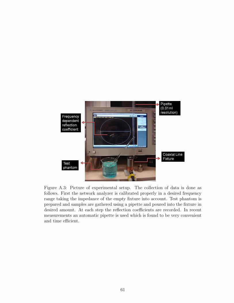
Figure A.3: Picture of experimental setup. The collection of data is done asfollows. First the network analyzer is calibrated properly in a desired frequencyrange taking the impedance of the empty fixture into account. Test phantom isprepared and samples are gathered using a pipette and poured into the fixture indesired amount. At each step the reflection coefficients are recorded. In recentmeasurements an automatic pipette is used which is found to be very convenientand time efficient.
61

Figure A.4: Results for dielectric measurements of some ionic solutions.
difference between the experimental and theoretical reflection coefficient values
at the desired frequency.
A.4 Results
Water solutions of different concentrations of NaCl and CuSO4 are measured
for their dielectric properties at two different frequencies: 123.5MHz and 64MHz
corresponding to Larmour frequencies at 3T and 1.5T static magnetic field, re-
spectively. The results are shown in Figure A.4. In-vitro rat blood sample
measurements are also done. At 123.5MHz εr=46.2 and σ=1.05S/m; at 64MHz
εr=67.5 and σ=0.955S/m.
Frequency dependence of the conductivity can be observed in Figure A.5 for
different concentrations of NaCl-water solutions and in Figure A.6 for varying
concentrations of CuSO4-water solutions. Subsequent measurement of the same
samples produced less than 0.3”%” error in εr and σ values.
62

Figure A.5: Frequency versus conductivity is plotted using real measurementsfor 6 different concentrations of NaCl and water solutions. Data is acquiredbetween 60MHz and 140MHz. The bottom line shows conductivity of pure water.Conductivity and permittivity for a wide range of frequencies can be measured atone experiment. This is a very important facility since there will be no need forinterpolation of the data due to lack of data at needed frequencies. Interpolationcan result in computation errors because the assumption linear dependence tothe frequency can be problematic specially if the interpolation range is long.
Figure A.6: Frequency vs. conductivity for CuSO4 and water solution of differentconcentrations. It is critical to form a data base for frequency and concentrationdependent dielectric properties of materials that one can use this data base toproduce a phantom of desired dielectric properties which could be used in safetyexperiments resulting in more reliable outputs.
63

A.5 Conclusions
In this study a measurement technique for determination of dielectric properties
is implemented with a cheap and practical setup. We have shown that solutions
of various relative permittivity and conductivity can be prepared by adjusting
the type and concentrations of the solutes inside. This property can be used for
preparation of MRI test phantoms that mimics dielectric properties of human
tissue and organs. Accurate knowledge of dielectric properties play significant
role in MRI safety studies.
64