Embed Size (px)
Citation preview
::t~tJA '#=-$' D '7
UILU-ENG-83-2010
~. I CIVIL ENGINEERING STUDIES STRUCTURAL RESEARCH SERIES NO. 507
ISSN: 0069-4274
A METHOD FOR THE COMBINATION OF STOCHASTIC TIME VARYING LOAD EFFECTS
By H. T. Pearce
Y. K. Wen
Technical Report of Research
Supported by the
NATIONAL SCIENCE FOUNDATION
Division of Civil & Environmental Engineering
(Under Grants CME 79-1S053 and CEE 82-07590)
UNIVERSITY OF ILLINOIS
at URBANA-CHAMPAIGN
URBANA, ILLINOIS
JUNE 1983


i 50272 ·101 REPORT DOCUMENTATION l,l.,~REPORT NO.
PAGE I UILU-ENG-83-2010 4. Title and Subtitle
12. Sponsorln" O'1lanlzatlon Name and Addr •••
I~ 3. Reclplent'a Accesalon No.
5. Repo'rt Date
JUNE 1983
(C) NSF CME 79-18053 ~)NSF CEE 82-07590
13. Type of Report & Period Covered ~ !
National Science Foundation ~
Washington, D.C. 1~ Ii
1----------'-------"-'-------'1
1
: 15. Supplemen"", No'.' .
·16. Abstract (Limit: 200 words)
The problem of evaluating the probability that a structure becomes unsafe under a combination of loads, over a given time period, is addressed. The loads and load effects are modeled as either pulse (static problem) processes with random occurrence time, inten~ sity and a specified shape or intermittent continuous (dynamic problem) processes which are zero mean Gaussian processes superimposed 'on a pulse process. The load coincidence method is extended to problems with both nonlinear limit states and dynamic responses, including the case of correlated dynamic responses. The technique of linearization of a nonlinear limit state commonly used in a time-invariant problem is investigated for timevarying combination problems, with emphasis on selecting the linearization point. Results are compared with other methods, namely the method based on upcrossing rate, simpler combination rules such as Square Root of Sum of Squares and Turkstra's rule. Correlated effects among dynamic loads are examined to see how results differ from correlated static loads and to demonstrate which types of load dependencies are most important, i.e., affect' the exceedance probabilities the most.
Application of the load coincidence method to code development is briefly discussed.
17. Document Analysis •. o.t.c:r1prOA
Load Combination, Extreme Values, Nonlinear Systems, Dynamic Effects, Random Processes, Random Vibration, Structural Reliability, Stochastic Dependencies
b. Identifiers/Open-Ended Terml
c. CQSATI Field/Group
18. Availability Statement
(See ANSI-Z39.18)
19. Security Class (This Report) 21. No. of Page:.
~UN~C~L~A~S_S __ I_F_I_E_D ________ ~ _____ 1_4_2 _______ ~ 20. Security Class (This Page)
UNCLASSIFIED See Instructions on Reverse
22. Price
OPTIONAL FORM 272 4-77) (Formerly NTIS-35) Department of Commerce


ii
ACKNOWLEDGMENT
This report is based on the doctoral thesis of H. T. Pearce
submitted in partial fulfillment of the requirements for the Ph.D.
in Civil Engineering at the University of Illinois. The study is
supported by the National Science Foundation under Grants
CME 79-18053 and CEE 82-07590. Their support is very much appre
ciated. Any opinions, findings and conclusions or recommendations
expressed in this report are "those of the authors and do not
necessarily reflect the reviews of the National Science Foundation.

CHAPTER
iii
TABLE OF CONTENTS
Page
INTRODUCTION •••••••••••••••••••••••••••••••••••••••••••••
1 • 1 1 .2 1 .3 1 .4 1 .5
Load Combination ••••••••••••••••••••••••••••••.••••• Problem Statement' Objectives of the Study Organization •••••••••••••••••••••••••••••••••••••••• Notation ........................................... .
1 4 4 5 6
2 MODELING AND LINEAR COMBINATION OF STATIC
3
LOAD EFFECT PROCESSES •••••••••••••••••••••••••••••••••••• 8
2. 1 The Poisson Pulse Process ••••••••• ,. • • • • • • • • • • • • • • • •• 8 2.2 Linear Combination of Load Effects
Modeled as Poisson Pulse Processes ••.•••••••••••••• 11 2.2.1 Exact Solutions •••.••••••••••••••••••••••••• 11 2.2.2 Approximate Methods ••••••.•••••••••••••••••• 13
2.3 The Method of Load Coincidence ••••••••••• '. • • • • • • • •• 16
NONLINEAR COMBINATIONS 'OF STATIC LOAD EFFECTS ........... 3. 1 3.2 3.3 3.4 3.5 3.6 3.7 3.8
3.9
In troduction ••.••••••••••••••••••••••••••••••••••.• The Load Effect Model •••••••.•••••••.•.•••.•••••... Mean Number of Outcrossings as Upper Bound ••••••••• Exact Crossing Rate for Poisson Pulse Processes Approximation by Linearization •••••••••••••••••.•.• Load Coincidence Method •••••••••••••••••••••••••••• Examples and Comparisons ••••••••••••••••••••••••.•• Other Methods for Calculating p .. ••••••••••••••••• 3.8.1 Multiple Checking POints1J
and Systems Approach •••••••.•••••••••••••••• 3.8 • 2 PNET Method ••••••••••••••••••••••••••••••••• Conclusions
20
20 21 21 22 23 27 29 32
32 32 33
4 MODELING AND COMBINATION OF DYNAMIC LOAD AND LOAD EFFECT PROCESSES ••••••••• e •••••••••••••••• 34
4.1 Introduction ••••••••••••••••••••••••••••••••••••••• 34 4.2 Intermittent Continuous Process
for Loads and Load Effects ••••••••••••••••.•••••••• 35 4.3 The Load Coincidence Formulation ••••.•••••••••••••• 37
4.3.1 Load Coincidence Solution as Upper Bound •••• 37 4.3.2 Computation of the Conditional Probabilities 38
4.4 Crossing Rate Methods •••••••••••••••••••••••••••••• 45 4.4.1 Point Crossing Method •••••••••••••.••••••••• 45 4.4.2 Shinozuka ' s Bound ••••••••••••••••••••••••.•• 46
4.5 Other Rules for Load Combination ••••••.•••••••••••• 51 4.5. 1 SRSS Rule ••••••••••••••••••••••••••••••••••• 51 4.5.2 Load Reduction Factor ••••••••••••••••••••••• 52

5
4.6
4.7 4.8
iv
Page
4.5.3 Turkstra's Rule •••••••••• m •••••••••••••••••• 52 4.5.4 Conclusions ••••••••••••••••••••••••••••••••• 53 Accuracy of the Conditional Failure Probability •.•• 54 4.6.1 First Passage Studies ••••••••••••••••••••••• 54 4.6.2 Errors in the 'Poisson Assumption •••••••••••• 56 4.6.3 Effects of the Mean Duration Approximation •• 58 Nonlinear Failure Surfaces ••••••••••••••••••••••••• 59 Inelastic Material Behavior •••••••••••••••••••••••• 60
CORRELATED LOAD EFFECTS 61
5.1 5.2 5. 3'
5.4
5.5
Introduction ••••••••••••••••••••••••••••••••••••••• Correlated Processes Within-Load Dependence •••••••••••••••••••••••••••••
Duration-Intensity Correlation •••••••••••••• Intensity Dependence •••••••••••••••••••••••• Occurrence Dependence (Clustering) .......... .
Between'Load Dependence •••.••••••••••••••••••••••••• 5.4.1 Intensity Dependence •••••••••••••••••••••••• 5.4.2 Occurrence Clustering among Loads ••••••••••• Conclusions ••••••••••••••••••••••••••••••••••••••••
61 62 64 64 66 68 69 69 71 74
6 APPLICATION TO STRUCTURAL CODES ••••••••••••••••••••••••• 75
7
6. 1
6.2 6.3
Introduction ••••••••••••••••••••••••••••••••••••••• 6. 1 • 1 6. 1 .2 6.1.3
Code Formats and Load Combinations Code Calibration •••••••••••••••••••••••••••• Adolescence •••••••••••••••••••••••••••••••••
Code Optimization •••••••••••••••••••••••••••••••••• Choice of the Target Reliability ..•.•••..........••
SUMMARY AND CONCLUSIONS
Summary ••••••••••••••••••••••••••••••••••••••••••••
Conclusions
75 75 78 78 79 84
87
87 88
FIGURES ••••...•.••...••..•• 0 •• G ••••• G • • • • • • • • • • • • • • • • • • • • • • • • • •• 93
APPENDIX
A TIME INVARIANT RELIABILITY MEASURES •••••••••••••••••••• 130 B THE RACKWITZ/FIESSLER ALGORITHM •••••••••••••••••••••••• 135
LIST OF REFERENCES ••••••••••••••••••••••••••••••••••••••••••••• 137

v
LIST OF TABLES
Table Page
Reliability Index for Different Load Ratios and Combinations •••••••••••••••••••••••••••• 82

vi
LIST OF FIGURES
Figure Page
2.1 Poisson Rectangular Pulse Processes ••••••••••••••••••••• 94
2.2 Combination of Ferry-Borges Processes .••••••••••••••••••• 95
2.3 Combined Sparse Poisson Pulse Processes ••••••••••••••••• 96
3.1 Vector Pulse Process with Nonlinear Domain •••••••••••••• 97
3.2 Crossing Rate Comparisons for 3 Linearization Points •••• 98
3.3 Vector Poisson Square Wave - Circular Domain •••••••••••• 99
3.4
3.5
Sparse Poisson Process - Circular
Interaction Curve for Beam Column
Domain •••••• ~ •••••••• 100
...................... 101
3.6 Crossing Rates for Beam Column ••••••••••••••••••••••••• 102
4.1 Intermittent Continuous Process •••••••••••••••••••••••• 103
4.2
4.3
4.4
4.5
4.6
4.7
~.8
4.9
4. '0
4.11
4 .. 12
Combined Nonstationary Processes ....................... Point Crossing Method - Direct and Conditional ......... Design Life Exceedance Probabilities · .................. Design Life Exceedance Probabilities · .................. Design Life Exceedance Probabilities · .................. Design Life Exceedance Probabilities · .................. Design Life 'Exceedance Probabilities · .................. Design Life Exceedance Probabilities · .................. Design Life Exceedance Probabilities · .................. Design Life Exceedance Probabilities · .................. Design Life Exceedance Probabilities · ..................
104
105
106
107
108
109
110
111
112
113
114
vii
Page
4.13 Conditional Failure Probability Pf(y) and Density fy(Y) •••••••••••••••••••••••••••••••••••• 115
4.14 First Passage Probability Solutions •••••••••••••••••••• 116
4.15 Errors in Overall Failure Probabilities using the Poisson Assumption ••••••••••••••••••••••••••• 117
4.16 Simulation Checking Mean Duration Assumption ••••••••••• 118
5.1 Between Process Intensity. Correlation Model •••••••••••• 119
5.2
5.3
5.4
5.5
5.6
5.7
5.8
Design Life Non-exceedan~e Probabilities
Design Life Non-exceedance Probabilities
Design Life Non-exceedance Probabilities
Design Life Non-exceedance Probabilities
Design Life Non-exceedance Probabilities
Design Life Non-exceedance Probabilities
Design Life Non-exceedance Probabilities
· ............. . · ............. . · ............. . · ............. .
· ............. .
120
121
122
123
124
125
126
5.9 Model for Occurrence Clustering •••••••••••••••••••••••• 127
5.10 Combined Nonstationary Earthquake and SRV Response ••••• 128
6.1 Exceedance Probabilities of LRF and Load Coincidence ••• 129

1
CHAPTER 1
INTRODUCTION
1.1 Load Combination
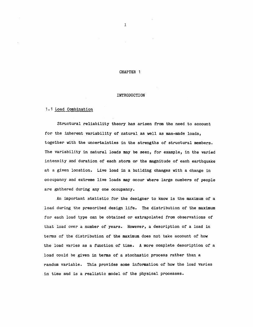
structural reliability theory has arisen from the need to account
for the inherent variability of natural as well as man-made loads,
together with the uncertainties in the strengths of structural members.
The variability in natural loads may be seen, for example, in the varied
intensity and duration of each storm or the magnitude of each earthquake
at a given location. Live load in a building changes with a change in
occupancy and extreme live loads may occur where large numbers of people
are gathered during anyone occupancy.
An important statistic for the designer to know is the maximum of a
load during the prescribed design life. The distribution of the maximum
for each load type can be obtained or extrapolated from observations of
that load over a number of years. However, a description of a load in
terms of the distribution of the maximum does not take account of how
the load varies as a function of time. A more complete description of a
load could be given in terms of a stochastic process rather than a
random variable. This provides some information of how the load varies
in time and is a realistic model of the physical processes.

2
The problem of "load combination" occurs when a number of different
loads, all of which are time varying, act on a structure during the same
time period. Design of a structure to withstand all the loads requires
the estimation of the maximum of the combined load process. When the
loads are modeled as stOChastic processes the solution is desired in
terms of the probability distribution of the maximum.
If the individual maxima were added, an extremely conservative
estimate of the maximum load would result because it is highly unlikely
that the maxima of all the processes occur simultaneously. Calculating
the distribution of the maximum of the combination of the stochastic
load (effect) processes is, however, complicated, particularly. for the
types of processes needed to model realistic loads.
Engineers in the design office generally rely on a code of practice
when designing civil structures under the combined action of loads. In
the past, probabilistic concepts were only used directly in codes to
specify characteristic loads for use in the analysis, the value of the
load being one which has only a small chance of being exceeded. Safety
factors incorporated in the allowable stress were used to provide the
margin of safety to ensure that the structure did not fail under the
wide range of loads. For cases where the design required a combination
of loads, a simple summation of the characteristic loads would result in
a very conservative design. The code writing committees therefore
provided simple rules (equations) to be followed in order to decrease
the combined maximum. These safety factors and combination rules were
based primarily on judgement. In a sense, the personalist concept
(Bunge, 1982) of probability was indirectly being used as a basis for
3
the safety factors in the codes. That is, the safety factors were based
largely on the beliefs (subjective as they may be, although attained
through much experience) of the members of the committee.
New codes are being proposed (e.g., Ellingwood, Galambos, MacGregor
and Cornell, 1980), using the concept of limit states design, which have
rational bases for obtaining load and resistance factors through the use
of the mathematical theory of probability. Of course, much data is
needed to compute the probability distributions of the random variables
and due to a scarcity of some data it is sometimes' necessary to use good
judgement in making certain assumptions. As more data becomes available
the distributions may be updated. The load and resistance factors will
reflect more accurately the relative uncertainty associated with each of
the variables.
Although buildings have generally behaved very well in the past
(designed using allowable stress), new materials are becoming available
and new facilities are being built with which we have little experience.
Knowledge gained from present studies on probability based design and
used in a rational way may help us to bUild, with confidence, these
innovative structures, as well as economizing by improving the design in
those situations where safety has been provided by ultra-conservatism.
A word of caution seems to be appropriate here. As in other
complex techniques in the engineering diSCipline, the use of probability
theory and the interpretation of the results should be accomplished with
insight and as much understanding of the problem as possible. We should
not attempt to get out of the analysis more than the input information
and model allow us.
4
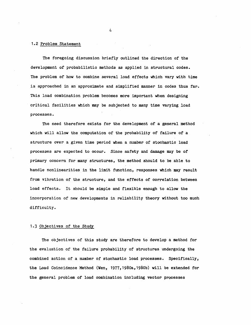
1.2 Problem Statement
The foregoing discussion briefly outlined the direction of the
development of probabilistic methods as applied in structural codes.
The problem of how to combine several load effects which vary with time
is approached in an approximate and simplified manner in codes thus far.
This load combination problem becomes more important when designing
critical facilities which may be subjected to many time varying load
processes.
The need therefore exists for the development of a general method
which will allow the computation of the probability of failure of a
structure over a given time period when a number of stochastic load
processes are expected to occur. Since safety and damage may be of
primary concern for many structures, the method should to be able to
handle nonlinearities in the limit function, responses which may result
from vibration of the structure, and the effects of correlation between
load effectsc It should be simple and flexible enough to allow the
incorporation of new developments in reliability theory without too much
difficulty.
1.3 Objectives of the Study
The objectives of this study are therefore to develop a method for
the evaluation of the failure probability of structures undergoing the
combined action of a number of stochastic load processes. Specifically,
the Load Coincidence Method (Wen, 1977,1980a,1980b) will be extended for
the general problem of load combination including vector processes
5
crossing out of nonlinear safe domains, dynamic load combinations, and
correlated effects.
The rules often suggested for combining stochastic loads for use in
developing structural codes or in the design of nuclear power plants are
compared with the results obtained from the load coincidence method to
evaluate the type of error being introduced when using these rules for
different risk levels.
A further objective is to give an appraisal and suggestions for
improvements of present practice in structural codes with regard to
reliability levels and internal consistency. Also the risk implications
of the load and resistance factor format will be studied~
1.4 Organization
Chapter 2 summarizes the methods of modeling of static loads or
load effects as random pulse processes and gives a review of results for
the linear combination of stochastic load processes. The Load
Coincidence method is briefly formulated.
Chapter 3 considers the problem of nonlinear combination, i.e., the
crossing of vector pulse processes out of nonlinear safe domains. As in
the case of time-invariant variables, an approximate method is to
linearize the failure surface at a suitably chosen point. Exact
crossing rates out of the linearized domain may be calculated. However,
computational effort may be excessive. The load coincidence method on
the other hand, is shown to be suitably versatile to handle efficiently
nonlinear combinations for various limit states and load types.
8
CHAPTER 2
MODELING AND LINEAR COMBINATION OF STATIC
LOAD EFFECT PROCESSES
2.1 The Poisson Pulse Process
The seemingly random occurrence of natural phenomena likely to
cause stresses in a structure suggests that arrival times of these loads
be points in a random point process. Beginning with the modeling of
floor live loads (Peir and Cornell, 1973) most reported load models for
loads which take on different magnitudes at different times (time
varying) assume the form of a filtered Poisson process. The Poisson
pulse process is a special form of this process and an efficient model
for static load effects in combination studies. It is a convenient
process for modeling a variety of loads which have independent arrival
times within one process. The occurrence times of the loads are given
by the points of a Poisson process having a mean rate of arrival of
-1 wh #l d' ere IJ. d is the mean duration of a load.
The load pulses occur between two renewal points and may assume a
number of shapes depending on the type of load being modeled. The most
widely used shape is the rectangular pulse, but triangles, house shapes
and sine waves have also been suggested. (Madsen, Kilcup and Corn~ll,

i 50272 -JOI REPORT DOCUMENTATION l.l ... k.
REPORT NO. PAGE UILU-ENG-83-20l0
4. Title and Subtitle
A HETROD FOR THE COMBINATION 9F STOCHASTIC TIME VARYING LOAD
3. Recipient'. Acce .. ion No.
5. RepOrt Date
JUNE 1983
i EFFECTS ~7-.-A-u-t-hO-~-S-)----------------------------------------·--~------------------------T-a--p-erl-o-nm--,n-&--o-~-a-n-,z-at-,o-n--Re-p-t-'-N-o'--~l!
H. T. Pearce, Y. K. Wen SRS No. 507 9. Perfonnlng O""anlzatlon Name and Address 10. Project/Task/Work Unit No. I
j
Department of Civil Engineering ~
University of Illinois 208 N. Romine Urbana, IL 61801
12. Sponsoring Organization Name and Add,....
National Science Foundation Washington, D.C.
15. Supplementary Notes
-16. Abstract (Limit: 200 words)
11. Contract(C) or Grant(G) No.
(C) NSF CME 79-18053 (mNSF CEE 82-07590
13. Type of Report & Period Covered
~----------------------------~ 14.
The problem of evaluating the probability that a structure becomes unsafe under a combination of loads, over a given time period, is addressed. The loads and load effects are modeled as either pulse (static pro·blem) processes wi th random occurrence time, intensity and a specified shape or intermittent continuous (dynamic problem) processes which are zero mean Gaussian processes superimposed ·on a pulse process. The load coincidence method is extended to problems with both nonlinear limit states and dynamic responses, including the case of correlated dynamic responses. The technique of linearization of a nonlinear limit state commonly used in a time-invariant problem is investigated for timevarying combination problems, with emphasis on selecting the linearization point. Results are compared with other methods, namely the method based on upcrossing rate, simpler I
combination rules such as Square Root of Sum of Squares and Turkstra's rule. Correlated effects among dynamic loads are examined to see how results differ from correlated static loads and to demonstrate which types of load dependencies are most important, i.e., affect' the exceedance probabilities the most.
Application of the load coincidence method to code development is briefly discussed.
~--------------------------------------------------------------------------------------------------------~ 17. Document Analysis B. Descriptors
Load Combination, Extreme Values, Nonlinear Systems, Dynamic Effects, Random Processes, Random Vibration, Structural Reliability, Stochastic Dependencies
b. Identifiers/Open-Ended Terms
c. COSATI Field/Group
18. Availability statement
(See ANSI-Z39.IS)
19. Security Class (This Report) 21. No_ of Page5
~UN~C~L=A=S~S~IF~I_E_D ________ ~_~~14_2 ______ ___ 20. Security Class (This Page) 22. Price
UNCLASSIFIED See Instructions on Reverse OPTIONAL FORM 272 (4-77)
(Formerly NTIS-35) Department of Commerce

ii
ACKNOWLEDGMENT
This report is based on the doctoral thesis of H. T. Pearce
submitted in partial fulfillment of the requirements for the Ph.D.
in Civil Engineering at the University of Illinois. The study is
supported by the National Science Foundation under Grants
CME 79-18053 and CEE 82-07590. Their support is very much appre
ciated. Any opinions, findings and conclusions or recommendations
expressed in this report are 'those of the authors and do not
necessarily reflect the reviews of the National Science Foundation.

CHAPTER
iii
TABLE OF CONTENTS
Page
INTRODUCTION •••••••••••••••••••••••••••••••••••••••••••••
1 • 1 1.2 1 .3 1.4 1 .5
Load Combination •••••••••••••••••••••••••••••••••••• Problem Statement' .................................... Objectives of the study Organization •••••••••••••••••••••••••••••••••••••••• Notation •••••••••••••••••••••••• , ••••••••••••••••••••
1 4 4 5 6
2 MODELING AND LINEAR COMBINATION OF STATIC
3
LOAD EFFECT PROCESSES ••••••••••••••••• 4 •••••••••••••••••• 8
2. 1 The Poisson Pulse Process ••••••••• ,. • • • • • • • • • • • • • • • •• 8 2.2 Linear Combination of Load Effects
Modeled as Poisson Pulse Processes ••••••••••••••••• 11 2.2.1 Exact Solutions ••••••••••••••••••••••••••••• 11 2.2.2 Approximate Methods •••••••.••••••••••••••••• 13
2.3 The Method of Load Coincidence ••••••••••••••••••••• 16
NONLINEAR COMBINATIONS ·OF STATIC LOAD EFFECTS
3. 1 3.2 3.3 3.4 3.5 3.6 3.7 3.8
3.9
Introduction ••••••••••••••••••••••••••••••••••••••• The Load Effect Model •••••••••••••••••••••••••••••• Mean Number of Outcrossings as Upper Bound ••••••••• Exact Crossing Rate for Poisson Pulse Processes Approximation by Linearization ••••••••••••••••••••• Load Coincidence Method •••••••••••••••••••••••••••• Examples and Comparisons ••••••••••••••••••••••••••• Other Methods for Calculating p.. • •••••••••••••••• 3.8.1 Multiple Checking Points~J
and Systems Approach •••••••••••••••••••••••• 3.8 .2 PNET Method ••••••••••.•••••••••••••••••••.•• Conclusions
20
20 21 21 22 23 27 29 32
32 32 33
4 MODELING AND COMBINATION OF DYNAMIC LOAD AND LOAD EFFECT PROCESSES •••••••••••••••••••••••••• 34
4.1 Introduction ••••••••••••••••••••••••••••••••••••••• 34 4.2 Intermittent Continuous Process
for Loads and Load Effects ••••••••••••••••••••••••• 35 4.3 The Load Coincidence Formulation ••••••••••••••••••• 37
4.3.1 Load Coincidence Solution as Upper Bound •••• 37 4.3.2 Computation of the Conditional Probabilities 38
4.4 Crossing Rate Methods •••••••••••••••••••••••••••••• 45 4.4.1 Point Crossing Method •••••••••••••••••••.••• 45 4.4.2 Shinozuka ' s Bound ••••••••••••••••••••••••••• 46
4.5 Other Rules for Load Combination ••••••••••••••••••• 51 4. 5. 1 SRSS Rule ••••••••••••••••••••••••••••••.•••• 51 4.5.2 Load Reduction Factor ••••••••••••••••••••••• 52
5
4.6
4.7 4.8
iv
4.5.3 Turkstra's Rule 4.5.4 Conclusions ••••••••••••••••••••••••••••••••• Accuracy of the Conditional Failure Probability •••• 4.6.1 First Passage Studies ••••••••••••••••••••••• 4.6.2 Errors in the 'Poisson Assumption •••••••••••• 4.6.3 Effects of the Mean Duration Approximation •• Nonlinear Failure Surfaces ••••••••••••••••••••••••• Inelastic Material Behavior ••••••••••••••••••••••••
Page
52 53 54 54 56 58 59 60
CORRELATED LOAD EFFECTS 61
5. 1 5.2 5.3
5.4
5.5
Introduction ••••••••••••••••••••••••••••••••••••••• 61 Correlated Processes ••••••••••••••••••••••••••••••• 62 Within-Load Dependence ••••••••••••••••••••••••••••• 64 5.3.1 Duration-Intensity Correlation •••••••••••••• 64 5.3.2 Intensity Dependence •••••••••••••••••••••••• 66 5.3.3 Occurrence Dependence (Clustering) ••••••.•••• 68 Between'Load Dependence •••••••••••••••••••••••••••• 69 5.4.1 Intensity Dependence •••••••••••••••••••••••• 69 5.4.2 Occurrence Clustering among Loads ••••••••••• 71 Conclusions •••••••••••••••••••••••••••••••••••••••• 74
6 APPLICATION TO STRUCTURAL CODES ••••••••••••••••••••••••• 75
7
FIGURES
APPENDIX
6. 1
6.2 6.3
Introduction ••••••••••••••••••••••••••••••••••••••• 6. 1 • 1 6. 1 .2 6.1.3
Code Formats and Load Combinations Code Calibration •••••••••••••••••••••••••••• Adolescence •••••••••••••••••••••••••••••••••
Code Optimization •••••••••••••••••••••••••••••••••• Choice of the Target Reliability
SUMMARY AND CONCLUSIONS
7 • 1 7.2
Su.mmary ••••••••••••••••••••••••••••••••••••••••••••
Conclusions
•••••••••••••••••••• O •• O ••••• G •••••••••••••••••••••••••••
75 75 78 78 79 84
87
87 88
93
A TIME INVARIANT RELIABILITY MEASURES •••••••••••••••••••• 130 B THE RACKWITZ/FIESSLER ALGORITHM •••••••••••••••••••••••• 135
LIST OF REFERENCES ••••• 0 • • • • • • • • • • • • • • • • • • • • • • • • • • • • • • • • • • • • • •• 137

v
LIST OF TABLES
Table Page
Reliability Index for Different Load Ratios and Combinations •••••••••••••••••••••••••••• 82

vi
LIST OF FIGURES
Figure Page
2G1 Poisson Rectangular Pulse Processes ••••••••••••••••••••• 94
2.2 Combination of Ferry-Borges Processes ,................... 95
2.3 Combined Sparse Poisson Pulse Processes ••••••••••••••••• 96
3.1 Vector Pulse Process with Nonlinear Domain •••••••••••••• 97
3.2 Crossing Rate Comparisons for 3 Linearization Points •• ~. 98
3.3 Vector Poisson Square Wave - Circular Domain •••••••••••• 99
3.4
3.5
Sparse Poisson Process - Circular
Interaction Curve for Beam Column
Domain •••••• ' ••••••••• 100
...................... 101
3.6 Crossing Rates for Beam Column ••••••••••••••••••••••••• 102
4.1 Intermittent Continuous Process •••••••••••••••••••••••• 103
4.2
4.3
4.4
4.5
4.6
4.7
~}. 8
4.9
4.10
4.11
lL 12
Combined Nonstationary Processes ....................... Point Crossing Method - Direct and Conditional ......... Design Life Exceedance Probabilities · .................. Design Life Exceedance Probabilities · .................. Design Life Exceedance Probabilities · .................. Design Life Exceedance Probabilities · .................. Design Life -Exceedance Probabilities · .................. Design Life Exceedance Probabilities · .................. Design Life Exceedance Probabilities · .................. Design Life Exceedance Probabilities · .................. Design Life Exceedance Probabilities · ..................
104
105
106
107
108
109
110
111
112
113
114
vii
Page
4.13 Conditional Failure Probability Prey) and Density fy(Y) •••••••••••••••••••••••••••••••••••• 115
4.14 First Passage Probability Solutions •••••••••••••••••••• 116
4.15 Errors in Overall Failure Probabilities using the Poisson Assumption ••••••••••••••••••••••••••• 117
4.16 Simulation Checking Mean Duration Assumption ••••••••••• 118
5.1 Between Process Intensity Correlation Model •••••••••••• 119
5.2
5.3
5.4
5.5
5.6
5.7
5.8
Design Life Non-exceedan~e Probabilities
Design Life Non-exceedance Probabilities
Design Life Non-exceedance Probabilities
Design Life Non-exceedance Probabilities
Design Life Non-exceedance Probabilities
Design Life Non-exceedance Probabilities
Design Life Non-exceedance Probabilities
· ............. . · ............. . · ............. .
· ............. .
120
121
122
123
124
125
126
5.9 Model for Occurrence Clustering •••••••••••••••••••••••• 127
5.10 Combined Nonstationary Earthquake and SRV Response ••••• 128
6.1 Exceedance Probabilities of LRF and Load Coincidence ••• 129
1
CHAPTER 1
INTRODUCTION
1.1 Load Combination
Structural reliability theory has arisen from the need to account
for the inherent variability of natural as well as man-made loads,
together with the uncertainties in the strengths of structural members.
The variability in natural loads may be seen, for example, in the varied
intensity and duration of each storm or the magnitude of each earthquake
at a given location. Live load in a building changes with a change in
occupancy and extreme live loads may occur where large numbers of people
are gathered during anyone occupancy.
An important statistic for the designer to know is the maximum of a
load during the prescribed design life. The distribution of the maximum
for each load type can be obtained or extrapolated from observations of
that load over a number of years. However, a description of a load in
terms of the distribution of the maximum does not take account of how
the load varies as a function of time. A more complete description of a
load could be given in terms of a stochastic process rather than a
random variable. This provides some information of how the load varies
in time and is a realistic model of the physical processes.

2
The problem of "load combination" occurs when a number of different
loads, all of which are time varying, act on a structure during the same
time period. Design of a structure to withstand all the loads requires
the es timation of the maximum of the combined load process. When the
loads are modeled as stochastic processes the solution is desired in
terms of the probability distribution of the maximum.
If the individual maxima were added, an extremely conservative
estimate of the maximum load would result because it is highly unlikely
that the maxima of all the processes occur simultaneously. Calculating
the distribution of the maximum of the combination of the stochastic
load (effect) processes is, however, complicated, particularly. for the
types of processes needed to model realistic loads.
Engineers in the design office generally rely on a code of practice
when designing civil structures under the combined action of loads. In
the past, probabilistic concepts were only used directly in codes to
specify characteristic loads for use in the analysis, the value of the
load being one which has only a small chance of being exceeded. Safety
factors incorporated in the allowable stress were used to provide the
margin of safety to ensure that the structure did not fail under the
wide range of loads. For cases where the design required a combination
of loads, a simple summation of the characteristic loads would result in
a very conservative design. The code writing committees therefore
provided simple rules (equations) to be followed in order to decrease
the combined maximum. These safety factors and combination rules were
based primarily on judgement. In a sense, the personalist concept
(Bunge, 1982) of probability was indirectly being used as a basis for

3
the safety factors in the codes. That is, the safety factors were based
largely on the beliefs (subjective as they may be, although attained
through much experience) of the members of the committee.
New codes are being proposed (e.g., Ellingwood, Galambos, MacGregor
and Cornell, 1980), using the concept of limit states design, which have
rational bases for obtaining load and resistance factors through the use
or the mathematical theory of probability. Of course, much data is
needed to compute the probability.distributions of the random variables
and due to a scarcity of some data it is sometimes necessary to use good
judgement in making certain assumptions. As more data becomes available
the distributions may be updated. The load and resistance factors will
reflect more accurately the relative uncertainty associated with each of
the variables.
Although buildings have generally behaved very well in the past
(designed using allowable stress), new materials are becoming available
and new facilities are being built with which we have little experience.
Knowledge gained from present studies on probability based design and
used in a rational way may help us to bUild, with confidence, these
innovative structures, as well as economizing by improving the design in
those situations where safety has been provided by ultra-conservatism.
A word of caution seems to be appropriate here. As in other
complex techniques in the engineering discipline, the use of probability
theory and the interpretation of the results should be accomplished with
insight and as much understanding of the problem as possible. We should
not attempt to get out of the analysis more than the input information
and model allow us.
4
1.2 Problem Statement
The foregoing discussion briefly outlined the direction of the
development of probabilistic methods as applied in structural codes.
The problem of how to combine several load effects which vary with time
is approached in an approximate and simplified manner in codes thus far.
This load combination problem becomes more important when designing
critical facilities which may be subjected to many time varying load
processes.
The need therefore exists for the development of a general method
which will allow the computation of the probability of failure of a
structure over a given time period when a number of stochastic load
processes are expected to occur. Since safety and damage may be of
primary concern for many structures, the method should to be able to
handle nonlinearities in the limit function, responses which may result
from vibration of the structure, and the effects of correlation between
load effects. It should be simple and flexible enough to allow the
incorporation of new developments in reliability theory without too much
difficulty.
1.3 Objectives of the Study
The objectives of this study are therefore to develop a method for
the evaluation of the failure probability of structures undergoing the
combined action of a number of stochastic load processes. Specifically,
the Load Coincidence Method (Wen, 1977,1980a,1g80b) will be extended for
the general problem of load combination including vector processes
5
crossing out of nonlinear safe dom~ins, dynamic load combinations, and
correlated effects.
The rules often suggested for combining stochastic loads for use in
developing structural codes or in the design of nuclear power plants are
compared with the results obtained from the load coincidence method to
evaluate the type of error being introduced when using these rules for
different risk levels.
A further objective is to give an appraisal and suggestions for
improvements of present practice in structural codes with regard to
reliability levels and internal consistency. Also the risk implications
of the load and resistance factor format will be studied~
1.4 Organization
Chapter 2 summarizes the methods of modeling of static loads or
load effects as random pulse processes and gives a review of results for
the linear combination of stochastic load processes. The Load
Coincidence method is briefly formulated.
Chapter 3 considers the problem of nonlinear combination, i.e., the
crossing of vector pulse processes out of nonlinear safe domains. As in
the case of time-invariant variables, an approximate method is to
linearize the failure surface at a suitably chosen point. Exact
crossing rates out of the linearized domain may be calculated. However,
computational effort may be excessive. The load coincidence method on
the other hand, is shown to be suitably versatile to handle efficiently
nonlinear combinations for various limit states and load types.
6
Chapter 4 develops the method for combinations of processes
consisting of dynamic structural responses and compares results with the
"crossing rate" methods together with approximate combination rules used
in structural codes.
Correlated dynamic effects are examined in Chapter 5. Correlation
may exist between load events within one process or between two
processes. Both these situations may be considered within the general
framework of the load coincidence method.
Chapter 6 comments on present code formats for load combination and
important considerations in developing new probability-based codes. An
optimized design technique with reliability constraints is suggested,
using the load coincidence method, for developing optimized codes and as
a design decision tool.
1.5 Notation
d
fX(x)
FX(x)
g(x)
L(t)
N+
P12
p[ ]
q
Q
duration of response
probability density function
probability distribution function
limit state (performance) function
reliability in (O,t)
number of crossings
conditional failure probability given coincidence
probability of [ ]
probability that a load is "on"
varying loads in the ANSI code
7
r threshold level So spectral density of white noise excitation
t time
Y random mean dynamic response
Z total dynamic response given occurrence
a load coincidence crossing rate
# reliability index
Y load factors
t percent critical damping
A mean arrival rate of loads in process i
~ mean load duration
v crossing rate
e lag time
p correlation coefficient
~ standard deviation
~ standard normal density
~ standard normal distribution
w frequency of structure
8
CHAPTER 2
MODELING AND LINEAR COMBINATION OF STATIC
LOAD EFFECT PROCESSES
2.1 The Poisson Pulse Process
The seemingly random occurrence of natural phenomena likely to
cause stresses in a structure suggests that arrival times of these loads
be points in a random point process. Beginning with the modeling of
floor live loads (Peir and Cornell, 1973) most reported load models for
loads which take on different magnitudes at different times (time
varying) assume the form of a filtered Poisson process. The Poisson
pulse process is a special form of this process and an efficient model
for static load effects in combination studies. It is a convenient
process for modeling a variety of loads which have independent arrival
times within one process. The occurrence times of the loads are given
by the points of a Poisson process having a mean rate of arrival of
-1 wh Il d' ere Il d is the mean duration of a load.
The load pulses occur between two renewal points and may assume a
number of shapes depending on the type of load being modeled. The most
widely used shape is the rectangular pulse, but triangles, house shapes
and sine waves have also been suggested. (Madsen, Kilcup and Corn~ll,

9
1979; Madsen, 1979). Successive loads have magnitudes (pulse heights)
which are independent and identically distributed random variables. The
pulse magnitude may, however, have a finite probability of being zero.
The magnitude, in this case, has a mixed probability density function,
with a discrete mass at zero and a continuous density for the other
values of the variate.
The density and distribution functions for a rectangular pulse
process are
f (s) s
F (s) s (1 - q) R(s) + qFX(s)
in which 6(s) = Dirac delta function, H(s) = step function, f and x
(2.1)
FX are the conditional density and distribution functions given the
magnitude is not zero. The real pulses (those with non-zero magnitude)
have a mean occurrence rate given by A = q I-L d 1 and the duration of the
load pulse has an exponential distribution. Consecutive "on lf or "off"
times are possible with this model, which is completely characterized by
the mean arrival rate It. of the pulses, the mean duration J.L d and the
conditional density function fX(x). To include effects of load
cor~elation the independence assumptiOns related to the occurrence time,
intensity, and duration may be relaxed. This has been the subject of
research in the reference by Wen and Pearce (1981), and is also
considered in Chapter 5 of this study.
10
Some loads, such as live loads in buildings, are always "on". For
such cases q = 1 and A = IJ. d 1 which means that A. IJ. d = 1. As the
product A I-Ld becomes smaller the process becomes more sparse, i.e., the
loads are infrequent or of shor~ duration or both. If IJ d tends to zero
while A remains finite, the pulses become "spikes" and the result is a
Poisson shock process (compound Poisson process). Sample functions of
the Poisson rectangular pulse process are shown in Fig. 2.1.
Derivations of the distribution functions of the magnitude at any time
for other pulse shapes may be found in the references by Madsen, Kilcup
and Cornell (1979) and Madsen (1979).
Other models which have been proposed result in similar sample
functions to those above, but lack a certain flexibility. Ferry-Borges
and Castanheta (1971) proposed a model in which each load history is
described as a sequence of rectangular pulses of fixed duration. The
pulse amplitudes are again independent and identically distributed. The
durations of such are required to be either a multiple or a factor of
one another, as shown in Fig. 2.2.
Madsen and Ditlevsen (1981) proposed an "on-off" Markov rectangular
pulse process. It consists of independent exponentially distributed
periods with constant random load, alternating with periods without
load. The "off" periods are also exponentially distributed with the
mean not necessarily the same as the "on" periods. The computation of
the crossing rate of sums of these Markov processes is given in the
above reference and is seen to be analytically complex.
11
2.2 Linear combination of Load Effects
Modeled as Poisson Pulse Processes
Prior research has been concerned mainly with the linear
combination of load processes. Some results of this research will be
reviewed briefly here, while extensions to nonlinear limit states and
dynamic loads will be examined in more detail later in the text.
The distribution of the load magnitude is denoted FX(xi) for the
ith load process (see Eq. 2.1). The pulse process. has a mean occurrence
rate A i and the mean duration of a load pulse will be J.L i. For a
Poisson square wave Ai J.l i = 1, whereas for a sparse process the magnitude
of the probability mass at zero will be 1 - Ai J.l i. FR (1", t) is the m
distribution of the maximum of the combined processes during the
interval O,t.
2.2.1 Exact Solutions
Few exact solutions for the combination of stochastic load
processes exist and these are limited to the linear combination of the
simplest load types. As described briefly in Section 1.1, the maximum
combined load usually determines the design load and therefore is the
one of interest to the engineer or the code writing committee. In
probabilistic terms, "solution" here means the computation of the
distribution of the maximum of the combined process.
12
The study of the time dependent nature of floor live loads (Peir
and Cornell, 1973) suggested they be modeled as a superposition of a
shock process and a Poisson square wave (PSW) process. Hasofer (1974)
obtained the distribution of the maximum of the sum of these processes
in the form
FR (r,T) m
-A T 2 e y(r,T) (2.2)
Y(r,T) is obtained as the solution to the Volterra integral equation
t
F(r,t) + '2 J F(r,t-u) y(r,u) du = y(r,t)
o (2.3)
where F(r,t) is the·distribution of the maximum during one pulse of the
PSW process
r
F(r,T) E f o
The subscript 1 denotes the shock process and 2 the PSW process.
(2.4)
Bosshard (1975) used a Markov process model to compute the maximum
of the sum of two PSW processes. The result is given in the form of an
infinite sum which requires significant numerical computation.
Gaver and Jacobs (1981) make use of the Laplace. transform method to
get the transform of the maximum of the sum of a shock and PSW process.
13
The Laplace transform of the maximum distribution is given by
(2.5)
where
r
M (~) x I (2.6)
o
Mean times to first passage are obtained as E[Tr ] = hx(O). Results are
given for specific distributions of the load magnitudes •.
George (1981) uses the same· technique to give results for shock and
PSW processes whose occurrences are dependent on those of the other
process.
The difficulties associated with computation·of these exact
solutions, together with their limitations as models for real loads
makes them less attractive in analysis or design of real structures
under combined loads. They do serve as good means of making comparisons
for approximate solutions.
2.2.2 ApprOXimate Methods
The maximum of the sum of N stochastic pulse processes wherein
coincidence between processes may be neglected (e.g., shock processes or
very sparse pulse processes) has the known distribution
FR (r,t) = exp _r-¥ A.t{l - FX (r)~ ~ FX (r) m ~=l 1. i J j=l j
(2.7)
14
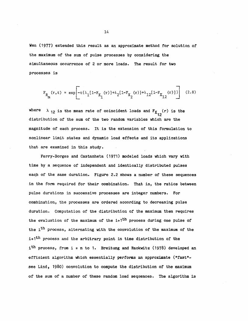
Wen (1977) extended this result as an approximate method for solution of
the maximum of the sum of pulse processes by considering the
simultaneous occurrence of 2 or more loads. The result for two
processes is
FR (r,t) m
where A 12 is the mean rate of coincident loads and FX (1") is the 12
distribution of the sum of the two random variables which are the
(2.8)
magnitude of each process. It is the extension of this formulation to
nonlinear limit states and dynamic load effects and its applications
that are examined in this study.
Ferry-Borges and Castanheta (1971) modeled loads which vary with
time by a sequence of independent and identically distributed pulses
eacp of the same duration. Figure 2.2 shows a number of these sequences
in the form required for their combination. That is, the ratios between
pulse durations in successive processes are integer numbers. For
combination, the processes are ordered according to decreasing pulse
duration. Computation of the distribution of the maximum then requires
the evaluation of the maximum of the i+1th process during one pulse of
the ith process, alternating with the convolution of the maximum of the
i+1th process and the arbitrary point in time distribution of the
ith process, from i = n to 1. Breitung and Rackwitz (1978) developed an
efficient algorithm which essentially performs an approximate (HfastH-
.see Lind, 1980) convolution to compute the distribution of the maximum
of the sum of a number of these random load sequences. The algorithm is
15
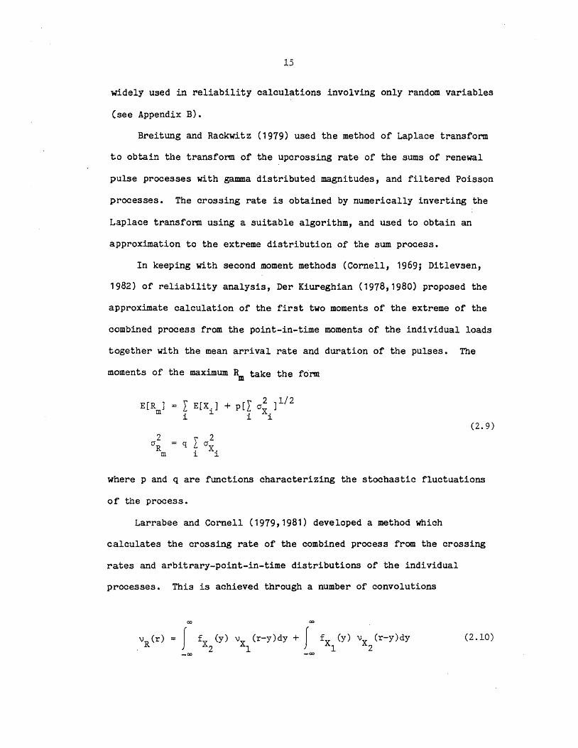
widely used in reliability calculations involving only random variables
(see Appendix B).
Breitung and Rackwitz (1979) used the method of Laplace transform
to obtain the transform of the upcrossing rate of the sums of renewal
pulse processes with gamma distributed magnitudes, and filtered Poisson
processes. The crossing rate is obtained by numerically inverting the
Laplace transfo~ using a suitable algorithm, and used to obtain an
approximation to the extreme distribution of the sum process.
In keeping with second moment methods (Cornell, 1969; Ditlevsen,
1982) of reliability analysis, Der Kiureghian (1978,1980) proposed the
approximate calculation of the first two moments of the 'extreme of the
combined process from the point-in-time moments of the individual loads
together with the mean arrival rate and duration of the pulses. The
moments of the maximum R take the form m
E[R ] I E[X. ] + p[~ 0"~.]1/2 m
i ~
~ ~
2 I 2 O"R q ax.
m i ~
(2.9)
where p and q are functions characterizing the stochastic fluctuations
of the process.
Larrabee and Cornell (1979,1981) developed a method which
calculates the crossing rate of the combined process from the crossing
rates and arbitrary-point-in-time distributions of the individual
processes. This is achieved through a number of convolutions
co co
f fxz (y) VX1
(r-y)dy + f fX (y) Vx (r-y)dy 1 2
(2.10)
-co -co
16
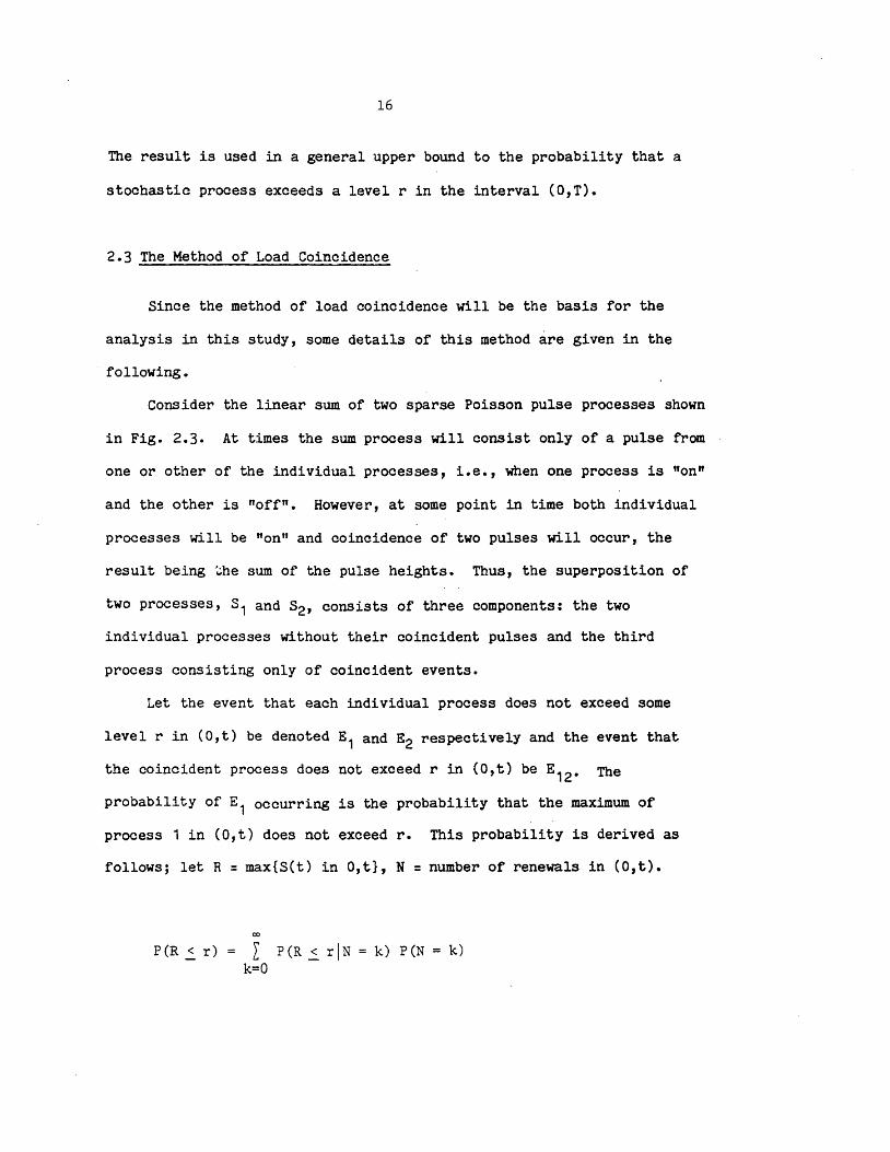
The result is used in a general upper bound to the probability that a
stochastic process exceeds a level r in the interval (O,T).
2.3 The Method of Load Coincidence
Since the method of load coincidence will be the basis for the
analysis in this study, some details of this method are given in the
following.
Consider the linear sum of two sparse Poisson pulse processes shown
in Fig. 2.3. At times the sum process will consist only of a pulse from
one or other of the individual processes, i.e., when one process is "on"
and the other is "off". However, at some point in time both individual
processes will be "on" and coincidence of two pulses will occur, the
result being ~he sum of the pulse heightse Thus, the superposition of
two processes, S1 and S2' consists of three components: the two
individual processes without their coincident pulses and the third
process consisting only of coincident events.
Let the event that each individual process 'does not exceed some
level r in (O,t) be denoted E1 and E2 respectively and the event tha~
the coincident process does not exceed r in (O,t) be E12e The
probability of E1 occurring is the probability that the maximum of
process 1 in (O,t) does not exceed r. This probability is derived as
follows; let R = max{S(t) in O,t}, N = number of renewals in (O,t).
peR 2 r) I peR ~ rJN k) peN k) k=O
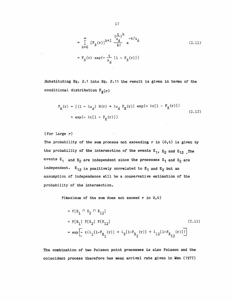
17
(2.11)
Substituting Eq. 2.1 into Eq. 2.11 the result is given in terms of the
conditional distribution FX(r)
(2.12)
= exp{- At[l - Fx(r)]}
(for large r)
The probability of the sum process not exceeding r in (O,t) is given by
the probability of the intersection of the events E1, E2 and E12 .The
events E1 and E2 are independent since the processes 31 and 32 are
independent. E12 is positively correlated to E1 and E2 but an
assumption of independence will be a conservative estimation of the
probability of the intersection.
P(maximum of the sum does not exceed r in O,t)
(2.13)
The combination of two Poisson point processes is also Poisson and the
coincident process therefore has mean arrival rate given in Wen (1977)
18
as
(2. 14)
Monte Carlo simulation in the above reference has verified this
occurrence rate for the coincident process. The occurrence rate of the
individual processes should be modified to account for the coincidences
The mean duration of the coincident pulses is also given by Wen as
l1d l1d 1 2
l1d + l1d 1 2
(2.15)
(2.16)
FX (r) is the distribution function of the sum of the amplitudes of the 12
two pulses, given the coincidence.
The load coincidence formulation for the combination of n
independent load effect processes may be written in the general form
1. - exp[- at]
n n n n n n
a. = I K.Pi
+ I L K. ,P. ,+ L L L AijkPijk i=l 1 i=l j=i+l 1J 1J i=l j=i+l k=j+l (2.17)
K A. A .. - Aik + A"k i 1 1J 1J
K •• A .. A"k 1J 1J 1J
where;
Pi = conditional probability of failure given
19
the structure is subjected to load i only = conditional probability of failure given
the coincidence of loads i and j
Ai = mean arrival rate of loads in process i
A. • = mean rate of co·incidence of loads in ~J
processes i and j
Aijk = mean rate of coincidence of loads in
processes i,j and k
Ki = mean occurrence rate of individual loads
without coincidence events
~j = mean duration of load in process j
The load coincidence method for linear combination of static load
effects has been shown to provide good results for a wide range of
parameters of the load processes (Wen, 1977,1980a). It is a
conservative approximation under certain conditions as shown in Section
4.3. The effect of the coincidence term is dominant at low risk (high
threshold) levels and therefore neglecting this term would introduce
significant error. Results have also been very favorably compared with
an exact solution for the combination of a Poisson square wave and a
Poisson spike process. The point crossing method of Larrabee and
Cornell (1978) generally gives results which are indistinguishable from
those of the load coincidence method for static load effects.
3.1 Introduction
20
CHAPTER 3
NONLINEAR COMBINATIONS
OF STATIC LOAD EFFECTS
The majority of the studies in load combinations thus far have
dealt with linear limit states; i.e.,. the limit (performance) function
g(X) is a linear function of the basic design variables (load effects
and resistance). This implies a linear response of the structure and a
linear resistance threshold. However, in many structural applications
the limit state function is a nonlinear function of these variables. A
nonlinear limit state may result for an elastic response of the
structure as in the case of lateral torsional buckling of a steel
beam-column. Nonlinear structural response must of course produce a
nonlinear limit state function.
If we consider a given resistance and plot the limit surface as a
function of the load effect variables, the problem may be visualized as
an n-component stochastic pulse process crossing out of a nonlinear
domain. This is the problem we will approach in this chapter without
specific regard to the way in which the nonlinearity arises.
21
3.2 The Load Effect Model
Consistent with the model described in Section 2.1, each component
process is modeled by one of the pulse processes used in linear
combinations. To visualize the·problem, Fig. 3.1a shows a perspective
sketch of two component samples of a vector process and the time
invariant limit surface. The mean arrival rate of the jth component
process is A j and the mean pulse duration is IJ. j •
3.3 Mean Number of OUtcrossings as Upper Bound
The probability that a ~neral stochastic process exceeds a
threshold in (O,t) (first excurs·ion problem) has not yet been obtained
analytically. An upper bound to this probability which provides a close
bound at high threshold levels may be derived as follOWS
Pf
P (at least one crossing occurs in O,t)
+ P[N (r,t) j]
< + j P[N (r,t) j]
+ - E(N (r,t)]
+ - \l (r)t
for a stationary process.
N+(r,t) = number of crossings in (O,t)
v+(r) = mean stationary crossing rate.
22
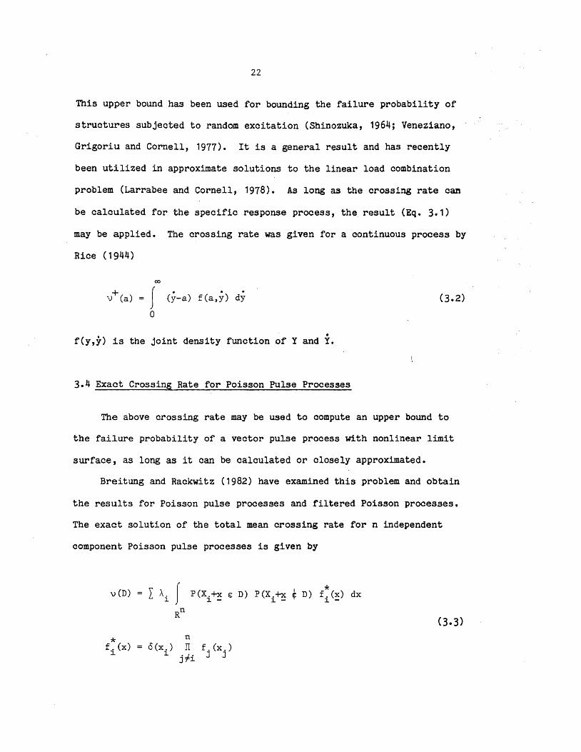
This upper bound has been used for bounding the failure probability of
structures subjected to random excitation (Shinozuka, 1964; Veneziano,
Grigoriu and Cornell, 1977). It is a general result and has recently
been utilized in approximate solutions to the linear load combination
problem (Larrabee and Cornell, 1978). As long as the crossing rate can
be calculated for the specific response process, the. result (Eq. 3.1)
may be applied. The crossing rate was given for a continuous process by
Rice (1944)
+ V (a)
00
J (y-a) f(a,y) dy
o
. f(y,y) is the joint density function of Y and Y.
3.4 Exact Crossing Rate for Poisson Pulse Processes
The above crossing rate may be used to compute an upper bound to
the failure probability of a vector pulse process with nonlinear limit
surface, as long as it can be calculated or closely approximated.
Breitung and Rackwitz (1982) have examined this problem and obtain
the results for Poisson pulse processes and filtered Poisson processes.
The exact solution of the total mean crossing rate for n independent
component Poisson pulse processes is given by
\) CD) I A. J P(X.+X E D) PCX.+x ~ D) * f. (x) dx
~ J. - J. - J. -
Rn (3.3)
* n
f. (x) cS (x. ) II f. (x.) 1 ~
j #i J J
23
where fj(Xj) is the probability density of the amplitude of the jth
component process and 0 the Dirac delta. The first term in the
integral is the conditional probability that the vector sum of the
components remains inside the safe domain D at a renewal of component i,
given the values of the other n-1 components. The second term is the
complement of the first. When n is larger than 2 this multiple integral
can become very costly. Under these circumstances an approximate
solution of the crossing rate becomes necessary.
3.5 Approximation by Linearization
Consider first the problem of calculating the probability content
of a nonlinear domain in time invariant reliability analyses. Hasofer
and Lina (1974) first suggested a solution in the form of a reliability
index which is defined as the smallest distance from the origin to the
failure surface in some normalized space. This is a purely second
moment solution.
When the distributions of the basic variables are known, an
approximate solution is obtained by linearizing the safe domain at a
suitable point on the failure surface. The success of this
linearization suggests a similar technique for approximately estimating
the crossing rate for a time varying load effect process. Linearizing
the failure surface permits the relatively easy calculation of the mean
crossing rate of the hyperplane rather than the complex nonlinear limit
surface.
24
The crossing rate given by Eq. 3.3 is simplified for the case of
Poisson renewal processes, with standard normal height distribution,
• crossing out of the hyperplane
n I a.i Xi - B = 0
i=l (3.4)
where ~ i are the direction cosines and (3 is the shortest distance from
the origin to the plane. The mean crossing rate becomes
n
L i=l
2 A.[~(S) - ~(S,S,l - a.)]
1 . 1
As in the time invariant case it is necessary to know at which
point the limit surface should be linearized in order to obtain as good
an approxima~ion as possible (Pearce and Wen, 1983). Breitung and
Rackwitz (1982) have addressed this problem by investigating points in
the time varying problem which are in several ways analogous to the
linearization point used in the time independent problem (see
Appendix A).
The first of these points is the point closest to the origin in a
transformed space. Tbe usual transformation is to a unit normal space.
In the time dependent problem the analogous pOint is still that point
closest to the origin. For time independent resistance variables and
stationary load processes, this point will remain unchanged with time.
The second 1s the point of maximum mean rate of crossing the
tangent hyperplane, suggested as being analogous to the pOint of maximum
likelihood (Shinozuka, 1983) or maximum probability content outside the
linearized safe domain in the time invariant case.
25
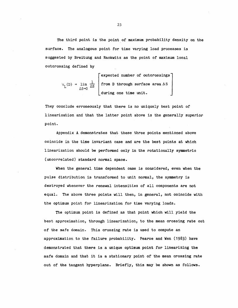
The third point is the point ,of maximum probability density on the
surface. The analogous pOint for time varying load processes is
suggested by Breitung and Rackwitz as the point of maximum local
outcrossing defined by
1. 1 ~m ~S
~S~ [
expected number of outcrOSSings]
from D through surface area AS
during one time unit.
They conclude erroneously that there is no uniquely best point of
linearization and that the latter point above is the generally superior
point.
Appendix A demonstrates that these three pOints mentioned above
coincide in the time invariant case and are the best points at which
linearization should be performed only in the rotationally symmetric
(uncorrelated) standard normal space.
When the general time dependent case is considered, even when the
pulse distribution is transformed to unit normal, the symmetry is
destroyed whenever the renewal intensities of all components are not
equal. The above three points will then, in general, not coincide with
the optimum point for linearization for time varying loads.
The optimum point is defined as that point which will yield the
best approximation, through linearization, to the mean crossing rate out
of the safe domain. This crossing rate is used to compute an
approximation to the failure probability. Pearce and Wen (1983) have
demonstrated that there is a unique optimum point for linearizing the
safe domain and that it is a stationary point of the mean crossing rate
out of the tangent hyperplane. Briefly, this may be shown as follows.
26
Let pU be the exact crossing rate out of the safe domain and v(XO)
the crossing rate out of the approximating hyperplane tangent at xc.
The error in the linearization is then given by
(3.6)
It is apparent that for largely convex safe domains ~those in which the
portion of the surface closest to the origin is convex and smooth), the
crossing rate out of the tangent plane. must be maximized for the error
to be minimized, because the tangent approximation will underestimate
the actual outcrossing rate. Conversely, when the limit surface of the
safe domain is largely concave, the crossing rate out of the tangent
plane overestimates the real crossing. rate and must therefore be
minimized for the error to be minimized.
The task of obtaining the local stationary points of the mean
crossing rate is a nonlinear programming problem which may be costly for
large dimensions. It also becomes increasingly difficult to locate the
best point when there are more than two stationary points. In this caae
it seems that the stationary pOint of the mean crossing rate closest to
the point of maximum local outcrossing will be the best point at which
to linearize the domain. The programming problem for this case becomes
increasingly difficult especially as the dimension increases.
Breitung and Rackwitz suggest that the point closest to the origin
(Hasofer/Lind point) may produce sufficiently accurate results for the
kind of limit surfaces found in structural mechanics. The examples in
Fig. 3.2 show results of the crossing rate out of the approximating
tangent hyperplane at the Hasorer/Lind point together with the point of
27
stationary mean crossing rate and the point of maximum local crossing
rate. For the convex safe domain in (a) (an ellipse), linearization of
the surface will obviously yield a poor approximation to the mean
crossing rate. However, as stated previously, the point of maximum mean
outcrossing rate provides the sharpest lower bound, i.e., it is the
optimum linearization point. In the special case of the ellipse,
wherein the process on the minor axis experiences the smaller renewal
intensity, and whose linearization at the point closest to the origin
(Hasofer/Lind) is, of course, parallel to the major axis, only crossings
by process 1 are possible. This explains the constant crossing rate
with increasing renewal intensity rate in (a). This linearization is
therefore very poor, but is certainly not generally so for all convex
safe domains.
For the concave safe domain in"(b) (a hyperbola) the point of
minimum mean outcrossing rate gives the closest upper bound as expected.
The point of maximum mean outcrossing rate does, of course, give results
which are extremely conservative as found by Breitung and Rackwitz. The
Hasofer/Lind point actually gives better results in this example than
the point of maximum local outcrossing.
3.6 Load Coincidence Method
The general formulation of the load coincidence method given in Eq.
2.17 is not restricted to linear limit states. For nonlinear limit
states and processes of the ki~d shown in Fig. 3.1 the occurrence and
coincidence rates are the same as in Eq. 2.17. The calculation of the
conditional failure probabilities becomes more difficult. For some
28
regularly shaped domains and certain load distributions the closed form
solution of the conditional probabilities may be possible. However,
where this is not possible some approximation to these probabilities is
necessary, as is currently the practice for time invariant reliability
problems.
The load coincidence method uses the Hasorer/Lind point in a
slightly different way from that suggested by Breitung and Rackwitz to
calculate the crossing rate. The term for the crossing rate is given as
for two load processes. The occurrence rates of the individual pulses
alone are given by K, and K 2 ; and of the coincident pulses by A12.
The -term Pi is the conditional probability that a single pulse will
exceed the limit state in the direction of· that component while no other
load is present. The conditional probability that the vector sum of two
component pulses, given coincidence, exceeds the limit state is P12.
The calculation of this probability is generally achieved, for
large dimensional nonlinear safe domains, through use of the Rackwitz-
Fieasler algorithm (Appendix B). The algorithm locates the optimum
linearization point (Hasorer/Lind point in unit normal apace) and the
approximate conditional probability of failure is given by
1. - <I>(B) (3.8)
where {3 is the dis tance of the point from the origin.
29
For sparse load processes the Hasofer/Lind point will give very
satisfactory results because it is unlikely that two pulses from one
process coincide with one pulse from another, destroying the symmetry of
the problem. The unsymmetrical nature arises when the renewal intensity
of one process is very different from that of another and the process is
dense. Many renewals of the one process may occur during just one
occurrence of the other.
For processes which are always on, the coincidence rate for the
load coincidence method is given by the sum of the individual renewal
intensities. The conditional failure probability may be calculated at
any instant of time as there is always coincidence. Calculation of the
crossing rate by the product of ·the coincidence rate and the conditional
failure probability implies that this probability at each.renewal of the
process with larger renewal intensity is independent of that at the
previous renewal. Clearly this is not true if no renewal of the other
process has occurred because its value is perfectly correlated until the
next renewal point. The approximation by independent pulses is a
conservative one and it retains the simplicity of the load coincidence
method.
3.7 Examples and Comparisons
The first example is a very nonlinear, but not really practical,
example. A two component renewal pulse process with unit normal pulse
height distribution crosses out of a centered circular domain. In this
particular example it is obvious that a single tangent hyperplane
approximation will yield results very different from the actual circular
30
domain. However, for this example, the exact probabilities are easily
calculated because of the fact that the sum of squares of normal
variates has a chi-squared distribution. The crossing rate obtained by
the load coincidence method is then given by
a.
where r is the radius of the circle and X2 is the chi-squared
probability distribution function.
Results for All =1 (always on) and All = 0.5 and 0.1 are shown in
figs. 3.3 and 3.4, respectively, together with the exact crossing rates
computed using Eq. 3.3. The load coincidence method gives increasingly
better results as the threshold increases and as the processes become
more sparse. When the radius is 3.0 and· A J.L = O. 1 no difference is
visible between the exact result and that of the load coincidence method
even for the very unsymmetrical case where A2» A1"
A second, more practical, example is given wherein a beam-column is
subjected to an axial load and end moments, both of which are modeled as
Poisson pulse processes. The interaction curve for buckling is shown in
Fig. 3.5 together with section sizes and properties. The curve (i.e.,
failure surface) is generally very close to linear, becoming noticeably
nonlinear only when the column is very slender.
The pulse amplitudes are assumed log-normal and the
Rackwitz/Fiessler algorithm using the prinCiple of normal tail
approximation is employed in order to estimate the conditional
probability of failure given that pulses from the two load effect
31
processes coincide. The safe domain in the original space is concave
which leads us to expect a conservative estimate of the conditional
probability of failure. However, the results show an unconservative
value which is due to the transformation of the failure surface to unit
normal space. The conservatism of the load coincidence method at low
thresholds and less sparse processes is greater than the unconservative
values of the probabilities and the overall effect is to give a
conservative result for the crossing rate. This can be seen in Fig. 3.6
where the exact crossing rates are also plotted for comparison. For
slightly higher thresholds and sparser processes the results become
unconservative but still compare well with the exact crossing rates.
The error on the unconservative -side will not be greater than that
produced by the transformation to normal space.
More complex examples with larger numbers of random components
(load and resistance) are more easily handled with the load coincidence
method. The conditional probabilities Pi' Pij are calculated without
much difficulty using the fast convolution technique of the Rackwitz
Fiessler algorithm or some method of nonlinear programming.
Random resistances are incorporated easily at the conditional
failure probability level, using the above technique, rather than
requiring the numerical integration of the total conditional probability
over the distribution of the resistance. This does however imply that
the resistance is independent tram occurrence to occurrence of a pulse,
which is an incorrect, but conservative, implication. Correlated load
effeots may aleo be considered and calculatior~ of Pij performed by
making use of a suitable transfo~tion as shown by Hohenbichler and
32
Rackwitz (1981).
3.8 Other Methods for Calculating Pij
3.8.1 Multiple Checking Points and Systems Approach
Linearization at just one point on the failure ~urface may not
approximate the safe domain sufficiently well for certain moderately
curved domains or when a large number of failure modes have to be
considered.
It is possible then to approximate the failure surface by the
intersection of a number of tangent hyperplanes enclosing a polyhedral
safe domain. The difficulty is to es·tablish the points at which the
planes are to be made tangential.
Ditlevsen (1982a) suggests this multiple point approximation for
systems with more than one mode of failure, each mode being linearized.
The reliability of the system is then given in the form of upper and
lower bounds obtained from system reliability techniques. The
hyperplanes are made tangent at the locally most dangerous point of each
mode, i.e., the stationary point of the distance of the orthogonal
projection point on the plane, from the origin.
3.8.2 PNET Method
Structures which fail in a ductile manner by forming plastic hinges
may be analysed by the PNET method developed by Ang and Ma (1979). The
method consists of two parts,
1. Identification of all significant modes
33
of collapse (failure mechanisms) 2. Synthesis of the probabilities of the
individual collapse mode to obtain the
system collapse probability.
In an earlier paper Wen (1980b) demonstrated the use and accuracy
of this method incorporated in the load coincidence formulation.
3.9 Conclusions
The load coincidence method provides a relatively simple extension
of some methods for time invariant reliability analysis to the very
complex problem of vector pulse processes crossing out of nonlinear
domains. Accuracy of the method is good especially for sparse
processes, but does depend on the accuracy of the conditional failure
probabilities and therefore on the shape of the domain.
Recently Grigoriu (1983) has proposed a method which approximates
the limit surface by some polynomial function of the basic variables.
Optimal estimates of the distribution of a control variable are obtained
to compute necessary probabilities. A linearization approach is also
proposed and said to be good for extension to time variant problems
using Turkstra's rule (see Section 4.5.3). The methods have not yet
been tested.
4.1 Introduction
34
CHAPTER 4
MODELING AND COMBINATION OF DYNAMIC
LOAD AND LOAD EFFECT PROCESSES
The forces of nature have challenged the engineer sinoe the first
structures were erected. The dynamic loads applied by these foroes
have, in the extreme, caused havoc and destroyed whole oommunities. But
the extreme loads are not the only ones causing damage. Combinations of
leas severe loads may be just as harmful.
Though predictions of environmental forces suoh as those due to
earthquakes and storms are subjects of ourrent research, the occurre~ce,
intensity and fluotuation of such forces are largely random. The
mathematical modeling of these loads is therefore best achieved by
probabilistic means, and the variation in time requires the use of the
theory of stochastio processes.
35
4.2 Intermittent Continuous Process for Loads and Load Effects
Dynamic loads are those loads which fluctuate with a time scale
close to the natural period of the structure causing severe changes in
the deformations and stresses. Examples of this type of loads are:
ground motion caused by earthquakes; wind; water waves; pressure
transients in nuclear reactors; shock or blast loads. Loads of this
type which occur in nature do so intermittently with long periods where
no such excitation, or excitation of such a low level to be unimportant,
will occur. Therefore the sparse Poisson process is suitable for
modeling the occurrence of such loads. However, in addition the loads
also fluctuate within each occurrence and therefore a more complex model
behavior than a rectangular pulse is required.
This is achieved by introducing a fluctuating process within the
duration of the pulse. This is done differently for two load types: the
zero-mean loads and the non-zero-mean loads.
Those loads, such as earthquakes and water waves, which have zero
mean are modeled by a continuous stochastic process whose expected value
is zero and variance function which is a measure of the magnitude of the
random fluctuation. During the total load process, the intensity of the
load will, in general, vary at each occurrence. The intenSity is
therefore a random variable. The spectral density of the random
process, which is related to the mean square value, thus has a random
fluctuation from occurrence to occurrence.
36
Loads such as wind pressure are composed of a mean or "static"
component and a gusting or fluctuating component. The mean component,
denoted Y and shown in Fig. 4.1, is allowed to vary at each load
occurrence and is therefore a random variable. The fluctuating
component is related to the mean component through its mean square
value. That is, it is proportional to the mean. The total load is thus
a superposition of a zero-mean continuous stochastic process X and a
rectangular pulse of magnitude Y. Such a composite random process is
hereafter referred to as an intermittent continuous process.
Any convenient process may be used to model the dynamic effect.
The processes used in this study are the Gaussian processes. "Many
physical processes, such as a steady sea state, turbulence in wind, as
well as ground acceleration can be approximately modeled by Gaussian
processes. Without loss of generality, in this study excitation is
modeled by Gaussian white noise for computational ease. More realistic
models can be introduced without analytical difficulty. For example, a
filtered white noise using a filter of the Kanai-Tajimi type is more
representative of earthquake motion than a modulated white noise and can
be used when analysing the response of a specific design to real ground
motion.
37
4.3 The Load Coincidence Formulation
4.3.1 Load Coincidence Solution as Upper Bound
The exact solution of the failure probability ,in (O,t) of a system
subjected to a stochastic load process requires a first passage
probability formulation and is very difficult to compute. The upper
bound in the form (see Eq. 3.1)
may be utilized in the reliability analysis. Consider a general Poisson
pulse process; let Pc be the probability of failure during one
occurrence, and A the rate of occurrence. The probability of failure
in (O,t) is then
Pf(t) ~ PfCD) + P Cat least one crossing in O,t)
(4.2)
This can be repeated for a combination of loads assuming the coincident
process to be independent of the others. The condition for the
inequality to hold is that A12 must be a conservative mean coincidence
rate, which it is (Wen, 1977).
38
The crossing rate (K,p + K2PC + A12P ) given by the load c 1 2 c 12 coincidence for.mulation therefore provides an upper bound to the failure
probability in unit time, so long as the conditional probabilities
Pc are computed exactly or estimated conservatively. i
In fact, the Poisson nature of the pulse process implies that the
Eq. 4.2(d) is a conservative value of the probability of failure in
(O,t). For combined dynamic load effects modeled as intermittent
continuous processes the load coincidence crossing rate is stated again
as
where now the Pi and Pij are conditional probabilities that the maximum
response during one load Occurrence or coincidence will exceed the
failure threshold. It is this probability, the probability of first
passage during the excitation, that we need to compute.
4.3e2 Computation of the Conditional Probabilities
The failure (first passage) probability during one load occurrence
or coincidence may be conservatively approximated from the crossing rate
of the failure threshold by assuming crossings occur independently and
are points in a Poisson process. Then the probability that no crossing
ooours in (O,t) is
L(t) exp[- v(r)t] (4.4)
and the failure probability Pr(t) = 1.-L(t). This result has been shown
39
to be asymptotically exact as r increases to infinity. Use of this
expression will be made because of its simplicity. Its accuracy will be
investigated later. If the process is nonstationary then Eq. 4.4
becomes
L(t)
t
exp[- J v(r,T)dTj
o (4.5)
For loads which can be represented as essentially stationary during one
occurrence a Gaussian white noise is used to model the excitation. The
spectral density So is constant over the frequency domain but is random
from load to load.
The stationary variance of -the response is
(4.6)
in which
t is the percent of critical damping.
w is the natural frequency.
The response of a linear system to a Gaussian input is also Gaussian,
and the crossing rate of level r is given by
v; J x fxi(r,~)d~ o
which for a stationary Gaussian process becomes
a· 2 + 1 x -r v = -- exp[-] r 2~ a 2 2 x (J
x
(4.7)
(4.8)
40
The stationary variance of the derivative of the response is
so that the crossing rate may be written
2 3 + = ~ e [-r ~w ]
'V r 271" xp 'ITS o
(4.9)
(4.10)
When the load may be more closely approximated by a modulated white
noise this is represented by
z(t) = <P(t) net)
in which, net) is a white noise process, ~(t) is a multiplier function.
The mean of z(t) is zero and its autocorrelation is given by
(4.11)
The statistics of the response, its variance and the variance of the
derivative function may be obtained in closed form, through lengthy
integrations, for certain multiplier functions (Lin, 1965). From the
above information, the rate of crOSSing a given threshold r at time t is
obtained as (Cramer and Leadbetter, 1967)
o. 2 1 x -r
'V ( r , t) :I: r:::- -;- exp [-2 ] {F } "2iT X 20 x
{F} n 4>(_n_) + h_p2
exp[ _n2
1 --i 12 & 2(1_0 2 )
pr n =
cr x
o o (t)
v1-0
Cov[x(t) x(t)] cr- (t) 0 (t)
x x
(4.12)
41
Then the probability of failure during the response of duration d is
given by
PI (r,d)
d
1. - exp[- J v(r,t)dt]
o (4.'3)
At each occurrence of a pulse in one load process the "intensity"
of the excitation, measured by the spectral density So, may differ from
the previous or any other occurrence. Therefore, in the model, the
measure of intensity is considered to be a random variable. In the case
of a non-zero mean process the static component may be modeled by a
random variable with the measure of intensity of the dynamic response in
some way related to the static value. Therefore p,(r,d) as given above
is a conditional probability, dependent on the spectral density S (which o
is related to the static component Y). For the non-zero mean case the
unconditional probability of failure during a pulse of mean duration
J.L d is
co ~d
[1 - exp{- J v;(t) [y=y dt}] fy(y)dy (4.14) J o o
which for the stationary response is
co
J (4.15)
o
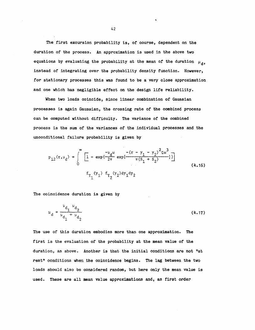
42
The first excursion probability is, of course, dependent on the
duration of the process. An approximation is used in the above two
equations by evaluating the probability at the mean of the duration ~d'
instead of integrating over the probability density function. However,
for stationary processes this was found to be a very close approximation
and one which has negligible effect on the design life reliability.
When two loads oOincide, since linear combination of Gaussian
processes is again Gaussian, the crossing rate of the combined process
can be computed without difficulty. The variance of the combined
process is the sum of the variances of the individual processes and the
unconditional failure probability is given by
(4.16)
The coincidence duration is given by
~d ~d 1 2
(4.17) ud ~d + ~d 1 2
The use of this duration embodies more than one approximation. The
first is the evaluation of the probability at the mean value of the
duration, as above. Another is that the initial conditions are not "at
rest" conditions when the coincidence begins. The lag between the two
loads should also be considered random, but here only the mean value is
used. These are all mean value approximations and, as first order
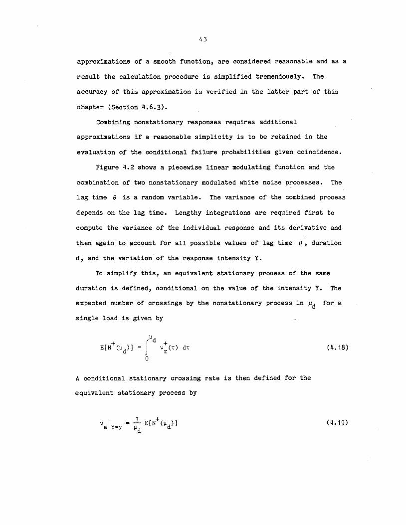
43
approximations of a smooth function, are considered reasonable and as a
result the calculation procedure is simplified tremendously. The
accuracy of this approximation is verified in the latter part of this
chapter (Section 4.6.3).
Combining nonstationary responses requires additional
approximations if a reasonable simplicity is to be retained in the
evaluation of the conditional failure probabilities given coincidence.
Figure 4.2 shows a piecewise linear modulating function and the
combination of two nonstationary modulated white noise processes. The
lag time () is a random variable. The variance of the combined process
depends on the lag timee Lengthy integrations are required first to
compute the variance of the individual response and its derivative and
then again to account for all possible values of lag time (), duration
d, and the variation of the response intensity Y.
To simplify this, an equivalent stationary process of the same
duration is defined, conditional on the value of the intensity Y. The
expected number of crossings by the nonstationary process in ~d for a
single load is given by
+ 'J ('r) dT
r
A conditional stationary crossing rate is then defined for the
equivalent stationary process by
'J I =.-l..E[N+C1.l)] e Y=y 1.ld d
(4.18)
(4.19)
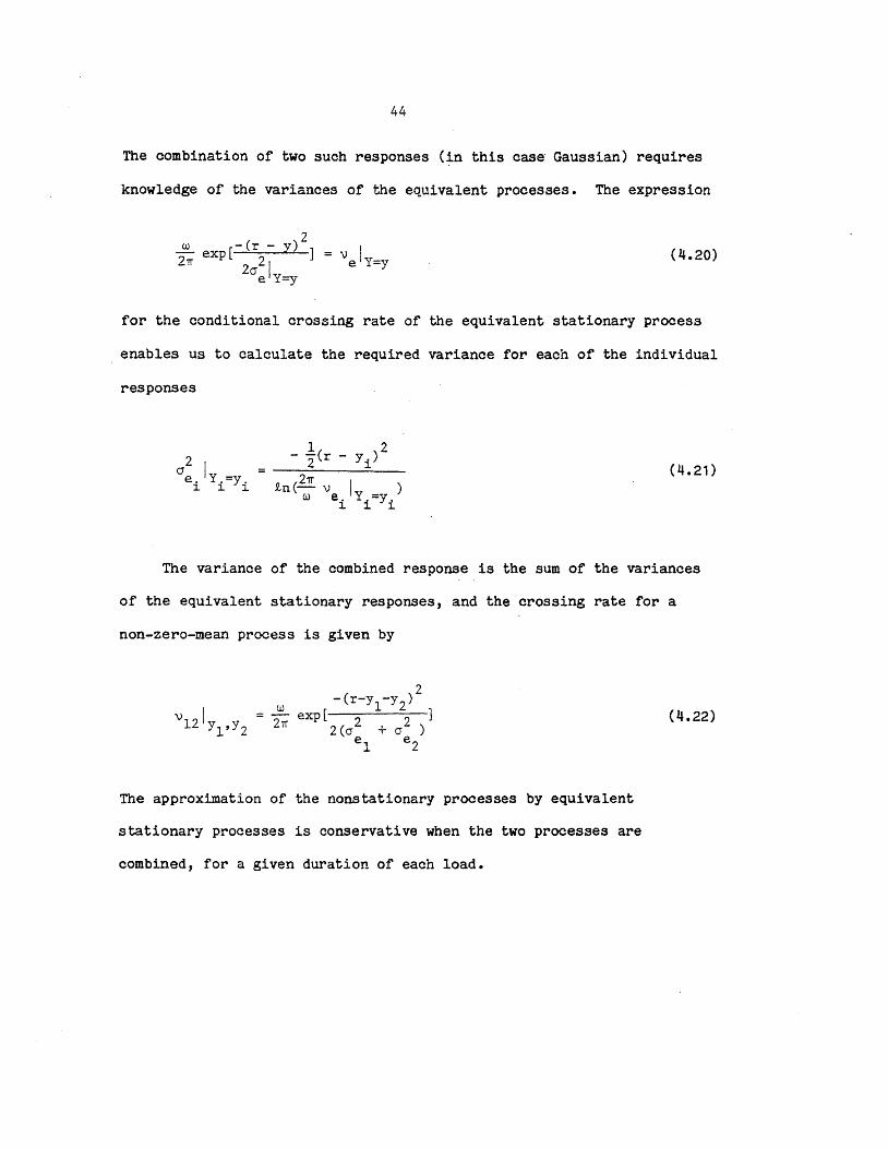
44
The combination of two such responses (~n this case' Gaussian) requires
knowledge of the variances of the equivalent processes. The expression
2 ~ exp[-(r - y) ] 2'Tr 2cr21
eY=y
(4.20)
for the conditional crossing rate of the equivalent stationary process
enables us to calculate the required variance for each of the individual
responses
02 I -e. Y.-y. ~ ~ ~
(4.21)
The variance of the combined response is the sum of the variances
of the equivalent stationary responses, and the crossing rate for a
non-zero-mean process is given by
(4.22)
The approximation of the nonstationary processes by equivalent
stationary processes is conservative when the two processes are
combined, for a given duration of each load.
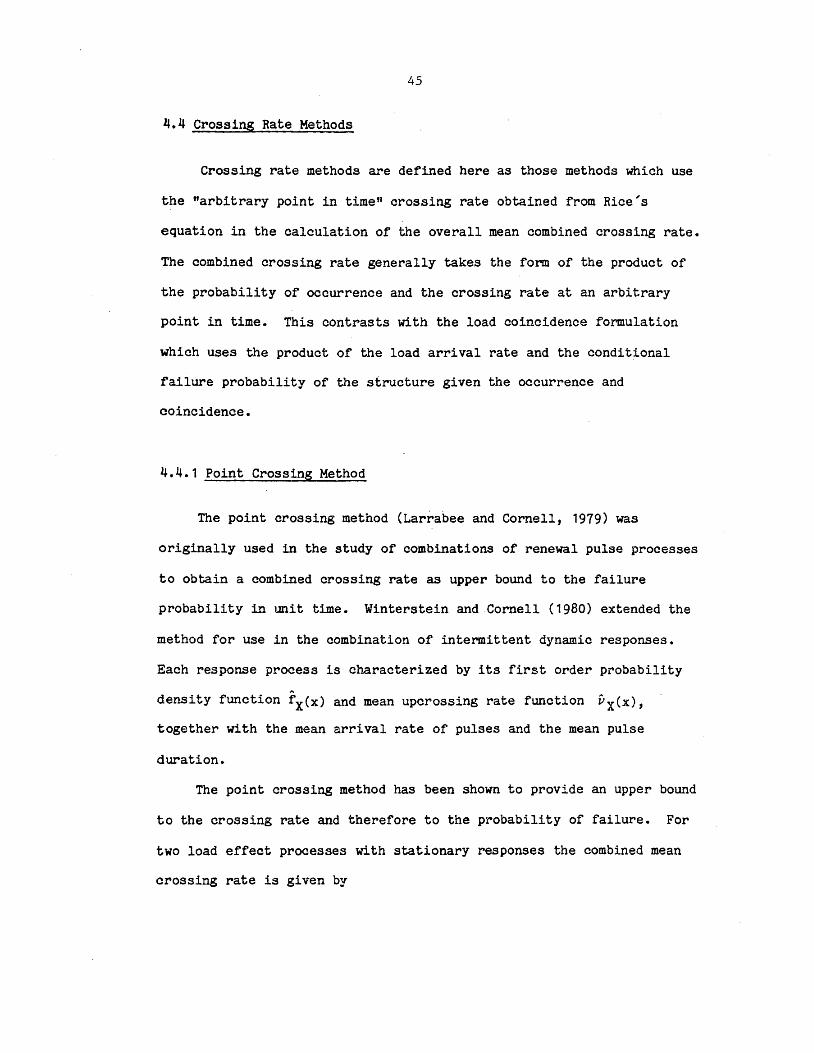
45
~.4 Crossing Rate Methods
Crossing rate methods are defined here as those methods which use
the "arbitrary pOint in time" crossing rate obtained from Rice's
equation in the calculation of the overall mean combined crossing rate.
The combined crossing rate generally takes the form of the product of
the probability of occurrence and the crossing rate at an arbitrary
pOint in time. This contrasts with the load coincidence formulation
which uses the product of the load arrival rate and the conditional
failure probability of the structure given the occurrence and
coincidence.
4.4.1 Point Crossing Method
The point crossing method (Larrabee and Cornell, 1979) was
originally used in the study of combinations of renewal pulse processes
to obtain a combined crossing rate as upper bound to the failure
probability in unit time. Winterstein and Cornell (1980) extended the
method for use in the combination of intermittent dynamiC responses.
Each response process is characterized by its first order probability
density function fX(x) and mean upcrossing rate function vX(x),
together with the mean arrival rate of pulses and the mean pulse
duration.
The point crossing method has been shown to provide an upper bound
to the crossing rate and therefore to the probability of failure. For
two load effect processes with stationary responses the combined mean
crossing rate is given by
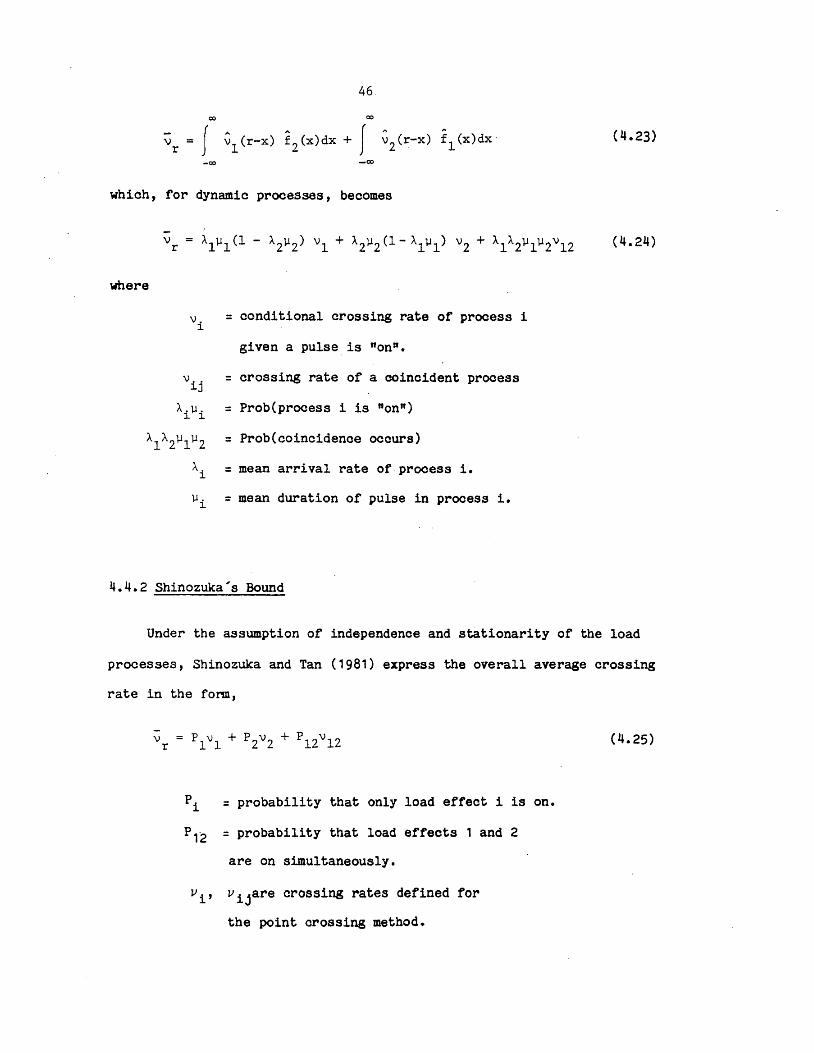
which,
where
46
co co
-J ~l(r-x) f2 (x)dx + J ~2(r-x) f1(x)dx· \)
r -co -co
for dynamic processes, becomes
-\)
r
Vi = conditional crossing rate of process i
given a pulse is "on".
Vij
= crossing rate of a coincident process
Ailli = Prob(process i is nonn)
AIA2111112 = Prob(coinc1dence occurs)
Ai = mean arrival rate of·prooess i.
lli = mean duration of pulse in process i.
4.4.2 Shinozuka's Bound
(4.23)
(4.24)
Under the assumption of independence and stationarity of the load
processes, Shinozuka and Tan (1981) express the overall average crossing
rate in the form,
(4.25)
Pi = probability that only load effect i is on.
P12 = probability that load effects 1 and 2
are on simultaneously.
vi' v ijare crossing rates defined for
the point orossing method.
47
Pi and Pij are calculated, for different load duration
distributions, from queueing theory. For two load processes wherein the
interarrival time between renewals and the load duration is
exponentially distributed, the above two methods arrive at the same mean
crossing rate, given in Eq. 4.24~
The combined mean crossing rate is conditional on the value of the
measure of intensity (spectral density) of the load processes. When
this intensity is uncertain,Wintersteln models the processes as the
product of a rectangular pulse process with constant (in time), but
random (from sample to sample), intensity A, and a stationary continuous
process Xet).
Both Winterstein and Shinozuka suggest the use of the Poisson
assumption, with crossing rate given in the form of Eq. 4Q24, to
approximate the first passage probability for the combined p~ocess.
Winterstein describes two ways in which the condition on the crossing
rate is removed by integration over the distribution of the intensity A.
The "direct" method removes the condition on the crossing rate (computes
expected crossing rate with respect to A) and uses the expected rate as
the crossing rate in the Poisson assumption for first passage
probability. The "conditional" method calculates a conditional failure
probability given the crossing rate and then evaluates the expected
probability by integration. The conditional method was found to give
better results for the situation modeled by Winterstein, in which A
remains constant throughout the process, but for the purpose of
comparison with the load coincidence formlation, the direct method is
48
used here since a realistic model should allow intensity variation from
occurrence to occurrence. The difference between the direct and
conditional methods is shown in Fig. 4.3.
The shortcoming of the crossing rate (Shinozuka, or Winterstein)
model is that, although the pulse intensity (or mean value) may be
considered random, the way it is modeled only allows. variation from
process to process and not from pulse to pulse within one process. For
example, an earthquake load process and a wind load process may have
different intensities but each occurrence within the earthquake process
will have the same intensity as the others using this model. The random
variable A controls the value of all the pulses within one process.
The load coincidence model does allow variation of the pulse
intensity within each process and is therefore a more physically
satisfying model.
If the upper bound to the conditional failure probability is used
in the load coincidence formulation (as the terms Pi' Pij) the point
crossing method (together with that of Shinozuka) and the load
coincidence method give similar results. However, when the crossings
occurring during each response pulse are assumed to be Poisson, and the
conditional failure probability is computed using this assumption,
considerable differences may arise for low thresholds and long load
durations, and also for high frequency oscillators (Figs. 4.4 through
4.12). The methods converge for high threshold levels and short load
duration when the period of the oscillator is large, say greater than
1.25 seconds. It may be worthwhile here to point out that the load
coincidence method generally yields conservative results indicating that

49
unde~ these circumstances the crossing rate method may yield results
which are unduly conservative.
Results are shown for stationary excitation in Figs. 4.4 through
4.12 for oscillators having natural frequencies of 3, 5 and 10 rad/sec
and 5% of critical damping. Implied probabilities of failure given by
use of the SRSS and Turkstra rule are also plotted. The methods of
calculating these probabilities are briefly described in the following
section. The Poisson assumption was used when evaluating the CDF of the
maximum for use in the above two methods. Comparisons are made
therefore, based on the relative magnitude of the probability given by
each method, acknowledging that the Poisson assumption yields a
conservative result in each case.
The graphs show how much more conservative the point crossing
method may be. In fact, only for the shorter durations and lowest
frequency considered is it less conservative than the SRSS value.
The differences between the methods may be explained by considering
the level at which the Poisson assumption i~ made. The point crossing
method calculates the mean crossing rate of the whole intermittent
dynamic response process and then assumes crossings occur as a Poisson
process over the whole design life. The load coincidence method assumes
that crossings during one pulse or coincidence occur as a Poisson
process and calculates the conditional probability of failure. Then,
using the fact that the pulses do indeed arrive in Poisson fashion, it
uses the conditional failure probability and the mean arrival rates to
evaluate the crossing rate of this process.
50
In addition to the Poisson assumption being used at different
times, two effects contribute to the sometimes significant difference
between the methods. The first is that for a given mean response the
difference between the methods increases as the threshold decreases.
The difrerence may be very large at small thresholds because the
orossing rate is large and if the duration is large ~ well, the upper
bound to the oonditional failure probability may be much greater than
unity 0 The use of the Poissonassumptlon in calculating the conditional
failure probability in the load coincidence method limits this
probability to being less than unity. At large thresholds the two
methods converge fairly rapidly.
The second effect is that the mean response level is a random
variable, in this case modeled by a gamma variate. The unconditioning
of the crossing rate or conditional failure probability is done by
weighting the conditional value by the probability density at that
level.
Figure 4.13 shows the conditional failure p,robability as a function
of the mean Y of the response. The probability density of Y is also
shown. The effeot of the weighting of the failure probability by the
density is to "spread" the differences between the two methods for the
case where only a single value of the mean response 1s considered. The
resulting differences are those shown in the Figs. 4.4 through 4.12.
51
4.5 Other Rules for Load Combination
Structural codes or recommendations use simpler and more
approximate methods to account for the fact that it is unlikely that the
maximum values of a number of loads will occur simultaneously. These
methods of evaluating the maximum design load take the form of a set of
rules to be applied by the designer. Essentially these rules reduce the
problem of the combination of random processes to that of random
variables. As a result, inaccuracies are introduced. The probability
of failure implied by these rules is examined here for comparison with
the results based on the more complete stochastic process models.
4.5.1 SRSS Rule
The square root of the sum of the squares (SRSS) rule has been
extensively studied and recommended (e.g., by Mattu and Nureg committee)
for combining two dynamic responses which coincide, but with random lag
time. The rule states that for two load processes S1 and S2;
where
R1 = max[S1(t)]
R2 = max[S2(t)]
(4.26)
It apears to give reasonably conservative results for a wide range of
combination situations. It is compared here with the load coincidence
method for use in computing the design life maximum of a number of
combined load processes.
52
For two processes the implied probability that the maximum Rm of
the combined process exceeds a level r is given by
where, for the case of dynamic response, we use
FR (r.) . J J
4.5.2 Load Reduction Factor
(4.27)
(4.28)
Some codp.s use a load reduction factor to reduce the total maximum
of two or more combined time varying loads. For example, in the ACI-318
concrete code, a factor of 0.75 is used when two loads such as live and
wind are together in a combination equation. It was found that a load
reduction factor of 0.7 has a safe domain very s'imilar to the SRSS
domain for two loads and any necessary conclusions will be drawn from
the results of the SRSS (Wen and Pearce, 1981b).
4.5.3 Turkstra's Rule
The developers of the new ANSI A58.1-1982 Minimum Design Loads have
applied Turkstra's rule when considering combinations of time varying
loads; i.eo, other than dead load.
53
The rule states that the maximum of the sum of two or more random
load processes is approximated by the sum of the maximum of process k
and the arbitrary point-in-time values of the other processes, with k
chosen to give the maximum of all n such combinations, n being the"
number of load processes. The advantage of this approximation is that
it uses only a random variable representation or the load processes.
However, the result is always an unconservative estimate of the maximum
combined load. As the maximum value and the arbitrary point in time
value are correlated, the evaluation of the implied probability is more
involved. Some details of the calculations for static load effects are
found in the paper by Wen (1980a).
4.5.4 Conclusions
It can be seen from Figs. 4.4 through 4.12 that, in general, the
type of load combination rules used in codes and described above are not
capable of giving consistent estimates of the combined maximum of a
number of intermittent continuous processes.
The SRSS rule is generally a conservative method for large risk
levels (low thresholds) but becomes an unconservative estimate at low
risk (high threshold) levels due to the failure to properly account for
the coincident load effect which dominates at high thresholds.
Turkstra's rule always gives an unconservative estimate of the
combined maximum, the accuracy of which depends more on the load
occurrence and duration characteristics than on the structural
parameters.
54
4.6 Accuracy of the Conditional Failure Probability'
In this chapter and the next, mention is often made of the
conditional probability of failure during the occurrence or coincidence
of dynamic loads. This may be stated as the probability that the
maximum of the response'process in (O,d) the duration of the response,
exceeds the limit state; or, the probability that the time to first
passage of the limit surface is less than d. Since the probability is
an important element in the combination analysis, it is of importance to
examine the accuracy of the method'used in this study and its effect on
the overall probability of combined load.
4.6.1 First Passage Studies
This problem of the time to first passage (crossing) of some level
by a linear oscillator experiencing random vibration has been
extensively addressed in the literature. Most studies have considered
the case of a Gaussian white noise excitation because the response (x,x)
is governed by a vector Markov process of dimension two. The joint
transition density function is obtained as the solution of the
Fokker-Planck equation (Lin, 1965).
Both numerical and approximate analytic approaches to the solution
of the failure probability have been attempted with varying degrees of
complexity and success. Simulation studies have also been undertaken
for comparison purposes. A discussion of these solutions and a good
list of references may be found in the works by Bergman (1979,1982) and
Yang and Shinozuka (1971,1972).
55
No simple approximate analytical procedure exists whereby
reasonably accurate results are achieved for a broad range of problems.
Bergman (1979) points out that a solution is available for the case
where the boundary conditions to the Fokker-Planck equation are natural,
i.e., no finite bounds on the displacement are prescribed. Then, for an
approximate solution to the first passage problem, the failure process
is modeled as an intersection between an unbounded distribution and a
deterministic threshold. Rice (1944) formulated the general equation
for the rate of upcrossing of a threshold by a random process, the
solution of which is easiest for the Gaussian process.
v(a) f (y-a) fYi(a,y)dy
o (4.29)
This result may be used in the simplest approximation to the first
passage distribution function by assuming that crossings of the level
occur independently and are therefore points in a Poisson process. This
solution is asymptotically exact as the threshold increases but for
small thresholds is very conservative.
In a narrow-band response the peaks of the process tend to occur in
clumps and are therefore not independent. It has thus been suggested
that the first passage probability would be estimated more accurately if
the crossings of the envelope of the process are considered independent.
Using the crossing rate of the envelope process given in Cramer and
Leadbetter (1967), the first passage probability thus obtained is still
a conservative estimate, but less so than the Poisson assumption.
Vanmarcke (1975) gives a slight improvement on the envelope crossing

56
rate by noting that there can be envelope crossings that are not
fOllowed by process crossings.
Bergman (1979) has recently solved the Pontriagin-Vitt equation for
the moments of time to first passage of the linear, and some nonlinear,
oscillators subject to a white noise excitation, using a finite element
technique. In subsequent studies (1982) he has obtained the numerical
solution to the transient problem of the probability of failure of the
oscillator subject again to white (or modulated white) noise excitation.
The reciprocal of the expected time to first passage isa good
approximation to the crossing rate though the probability so obtained
using an exponential distribution is generally unconservative."
The results for dynamic combination in this study are all obtained
using the assumption of Poisson crossings for the approximate
conditional first passage probability, given the occurrence or
coincidence of a load pulse. This is done because the probability is
simply expressed in analytic form and because the probabilities of
interest are connected with high threshold levels. The probability
density function of the first passage time is also obtainable and is
required for the calculations of the probabilities implied by the SRSS
and Turkstra methods.
4.6.2 Errors in the Poisson Assumption
It is necessary to try to evaluate the errors which might occur for
the design life failure probability when the Poisson assumption is used
in the conditional first passage probabilities.
57
It is, at present, not feasible to incorporate the finite element
solution in the load combination problem because of the number of times
a solution is required for the case where the intensity and lag times
are random variables.
A very close (and conservative) approximation to the first passage
probability has been obtained empirically by Lutes, Chen and Tzuang
(1980) by fitting curves to simulation results for different values of
the percent of critical damping. The form of the solution for the
failure probability is
t
1. - exp[- f n(T)dT]
o (4.30)
With thp results obtained by Bergman, avoiding the need for simulation
and providing a much broader data base, a still better empirical fit is
now possible.
However, the result given by Lutes is used in this study to examine
the overall effect of the Poisson assumption. Figure 4.14 shows a
comparison of the failure probability of a linear structure subjected to
a white noise excitation, for low thresholds, given by the Poisson
assumption, Vanmarcke's approximation, Lutes' empirical fit, and
Bergman's finite element solution.
Both Vanmarcke's approximation and Lutes' result have been used for
the conditional probability in the load coincidence calculations and the
comparison with the Poisson assumption is shown in Fig. 4.15. For the
design life failure probability the difference between Vanmarcke's and
Lutes' methods is not visible and the Poisson assumption provides
58
sufficiently close yet conservative results.
4.6.3 Effects of the Mean Duration Approximation
In Section 4.3.2 mention was made of the use of the mean duration
in calculating the conditional failure probabilities. It can be shown
analytically that for a given mean (static) component, the use of the
mean duration in the evaluation of the probability is conservative for
exponentially distributed duration. The same can be done for the
coincident loads assuming a gamma distribution for the coincident
duration as it is no longer exponential.
To support this statement, without details of the analysis, a Monte
Carlo simulation was perfonmed. Two Poisson processes of mean
occurrence r?tes A1 and A2 are first simulated. For each load
occurrence (point in the Poisson process) an exponentially distributed
duration, and a gamma distributed static component are generated. Due
to the excessive cost of simulating continuous processes at each
occurrence, the assumption of Poisson crossings is used to simulate the
maximum of the dynamic response for the actual load and coincident
durations. The maximum of the combined process is found and the
procedure repeated for the required sample size. The simulation results
(circles) are plotted in Fig. 4.16 together with the results obtained
analytically (solid line) using the load coinCidence method. The good
comparison provides validity for the use ot the mean duration (a first
order approximation) in the computations.
59
4.7 Nonlinear Failure Surfaces
For failure surfaces defined by some nonlinear function of the
basic variables the problem becomes one of a multi-dimensional
continuous process exiting the safe domain. The conditional probability
or failure given occurrence and coincidence can be evaluated using the
Poisson approximation, if the outcrossing rate can be obtained.
The crossing rate out of the safe domain may be given by a
generalization of the result given by Rice (1944)
00
(Belyaev, 1969).
x f • (x.,~ )d~ n ~,xn - n n (4.31)
Veneziano, Grigoriu and Cornell (1911) have utilized this result
and specialized the problem to Gaussian processes crossing out of
certain regularly shaped domains.
The simplest approximation for the general nonlinear surface is to
linearize it at just one point and approximate the real crossing rate by
the rate of crossing the tangent hyperplane. The result for Gaussian
processes is
(4.32)
The point at which the linearization should be performed is the point on
the surface at which vn becomes stationary (either maximum or minimum,
depending on the shape of the domain) and is found by an appropriate

60
nonlinear programming technique.
If the domain is known to be better approximated by other shapes
such as rectangles or circles, similar results are given for the
crossing rates in Veneziano, et al., (1977).
4.8 Inelastic Material ·Behavior
Structures which undergo inelastic deformations (eg. hysteretic
behavior) while subjected to random vibration have been treated by using
the method of equivalent linearization (Wen, 1980a). Calculation of the
first passage probability is achieved by use of the above-mentioned
approximations for the equivalent linear systems. Accuracy of the
results of the load coincidence formulation will depend on the accuracy
obtainable th~ough the linearization technique and the first passage I
approximation.
61
CHAPTER 5
CORRELATED LOAD EFFECTS
5.1 Introduction
The loads considered thus far have been modeled by independent
processes. Many loads may show correlation between occurrence times,
duration and intensity. An earthquake of large magnitude is usually
longer than one of lesser magnitude. The same may be said for a storm.
The wave height in a storm at sea is dependent on the intensity of the
wind. In the design of nuclear power plants there has been much
discussion as to whether a design basis accident load such as a large
LOGA could be caused by an earthquake, thereby introducing dependence of
the LOCA on earthquake occurrence and intensity. For example, Stevenson
(1980) argues that the present practice of allowing only one pipe break
to occur for a given earthquake is a non-rational constraint. For if
the earthquake could cause a pipe break, even when the piping is
specifically designed to resist seismic movements, then it would be
quite possible for more than one break to occur considering the amount
of piping present in the plant. If no dependence is considered and the
LOCA and earthquake are assumed independent then the probability of
simultaneous occurrence is so small as to be ignored for usual deSign
62
basis extreme loads.
We note that even for piping designed to resist an earthquake,
there is still a small probability of a break occurring and that this
probability and the resulting combined loads ought to be examined.
An event which certainly can be triggered by an earthquake is the
release of pressure from a Safety Relief Valve (SRV).in a Boiling Water
Reactor (BWR), producing a high probability of the effects of the two
loads being combined.
This type of dependent load effect may be modeled with correlated
stochastic processes in order to solve for the maximum of combined
processes.
Motivation for proposing correlated models is given by the need for
a realistic treatment of the dynamic effects experienced by important
structures under natural hazards, in particular, Nuclear Power plants
(Schwartz, Ravlndra, Cornell and Chou, 1980; Ravindra, 1980).
5.2 Correlated Processes
Correlation amongst static load effect processes, in terms of
occurrence time, duration and intensity, has been considered for linear
combinations of rectangular pulse processes in Wen and Pearce (1981).
For dynamiC load effects the correlation between individual responses is
considered here by assuming that the mean values Y of the response
processes exhibit dependent behavior. When the process has a mean of
zero, dependence is assumed between the measures of intensity (spectral
density) of the loads.
63
In the following, the additional modeling required for dynamic load
e~fect processes is described. The models describing the correlation
structure, and much of the analysis, generally follows that in Wen and
Pearce (1981). Two general types of dependence will be considered; (1)
Within-load dependence in which correlation exists only between the
parameters of one load type, (2) Between-load dependence in which the
parameters of one load process are correlated with those of another.
The form of the load coincidence equation remains essentially the
same as in Eq. 2.17 though now the occurrence rates and conditional
probabilities will be modified to account for the correlation. They
will not always be separable as in the independent case.
It is convenient to define the conditional distribution of the
maximum response during the pulse of duration d, given the mean value Y,
as
S(rly) 2 3
{ dw [-(r-y) ~w ]} exp - 21l" exp 1l"S
o
and for the coincident loads
2 3 -(r-y -y ) ~w dw 1 2 ] }
exp{- 21l" exp[ 1l"(5l
+ 52)
Except for the case of individual pulses with duration-intensity
(5.1)
(5.2)
dependence, the expected value of S(rly) with respect to the duration d,
will be approximated by S(rly) evaluated at the expected duration.
64
5.3 Within-Load Dependence
Loads from two simultaneously occurring processes are assumed to be
statistically independent of each other, but occurrence times, duration
and intensity of loads within one proCess may be correlated.
5.3.1 Duration-Intensity Correlation
Certain natural loads exhibit correlation between their duration
and intensity, e.g., intense storms will last longer than minor ones.
The occurrence times are assumed independent and therefore the
individual occurrence rates Ki remain unchanged from Eq. 2.17~
However, since a longer duration implies a larger coincidence rate and a
higher probability of maximum response, the coincident crossing rate
AijPij will change, but the two terms may not be considered separately.
The maximum dynamic response depends on the duration and therefore the
individual conditional failure probability will also be altered.
The duration and intensity of the static component are assumed to
be jointly normal, for computational ease, although the duration is
usually assumed exponential. This approximation should have negligible
effect when sparse processes are considered.
The failure probability, given the occurrence, for a load without
coincidence is
65
The mean crossing rate for the coincident pulses is given, for bivariate
normal duration and intensity, by
00
(5.4) 00
in which
00
L(r/Y1) f S(r/ y1
,y2) fy (Y2) dY2 0
2
(5.5) aD Y1 - lly
M1 1 + p 1 ( 1)
D1 'Y1 ay II .
1 DI
Pd,y is the correlation coefficient between D and Y.
The results of this dependence on the.non-exceedence probability
(NEP) are plotted on type-I extreme probability paper together with the
independent case (Figs. 5.2 through 5.8). The values of the parameters
used are E[Y] = 1. and ~y = 0.3
The duration-intensity dependence yields a probability, of not
exceeding a certain level, smaller than the independent case, ie., a
higher maximum combined response is expected. Use of an independent
assumption means that an unconservative estimate of the maximum is
obtained. However, this difference is small, e.g., at high thresholds
the ratio of the dependent failure probability to the independent is
66
only about 1.3 for an almost perfect correlation ( p = 0.99) Therefore
this correlation may not affect a design significantly.
5.3.2 Intensity Dependence
For example, the intensity of pressure transients, in nuclear
systems, caused by discharge of a relief valve due to buildup of
pressure may depend on the intensity of the previous transient.
This dependence between load pulses in a single process is achieved
by imbedding a Gauss- Markov sequence in the pulse process. The value
of the mean component of one pulse is dependent on the value of the mean
of the previous pulse as follows
Y k+ 1 p Yk + h - p 2
V k (5.6)
Yk is the mean of the kth pulse in the process. Vk 1s an independent
normal variate with E[V] = E[Y] /(1-p )/(1+p) and (Iv = (Iy.The
correlation structure is completely specified by the coefficient p.
Let the maximum response in a single pulse, the sum of the static
and dynamic components, be Zi for the ith pulse. Then the conditional
probability distribution of Z2 given Z1 is
in which
J o
GO
FZ Z (r,r) 2 1 (5.7)
FZ Z (r,r) 2 1
co co
J J o 0
67
(5.8)
where S(rly) is the probability 'that the maximum response is less than r
given that the load intensity is y (Eq. 5.1).
The joint density is derived from the product of a conditional
density and a marginal density. The conditional density is obtained
from the relationship given in Eq. 5.6
Y - Y f (2 1)
VI ~ 2 1 - P
1 11:2 - PY1 - (1-P)~l2 --- exp{- -L J } /2; cry 2 / 2
(1 - P cry (5.9)
Considering the Poisson character of the occurrence of load pulses,
the probability of the maximum in T years of a single process of
non-coincident pulses not exceeding a threshold r, is given
approximately by (Wen and Pearce, 1981)
FZ (r)
peRl ~ r) ~ L(z~IZ1) exp{- Klt[l - L(Z2IZ1)]} (5.10)
68
The coincident pulse sequence is also treated as Markovian and an
equivalent one-step correlation coefficient is computed from the
parameters of the individual processes and the coincidence rate.
The non-exceedance probability P(R12 ~ r) of the coincident process
is then obtained in a manner similar to that above and the combined NEP
may then be given by the product
NEP = peRl ~ r) P(Rz ~ r) P(RI2 ~ r)
For correlation coefficients less than 0.9 there is no visible
difference between the dependent and independent cases. As the
(5.11)
coefficient goes from 0.9 towards 1.0 the difference increases at low
thresholds but the independent results are always conservative. For
perfect correlation ( p = 1.0) all the pulses in the process have the
same static component and the exceedance 'probability is greatly reduced
at low thresholds (Figs. 5.2 to 5.8).
5.3.3 Occurrence Dependence (Clustering)
For example, safety relief valves are triggered in clusters in
order to discharge the pressure buildup in a BWR containment. Clusters
of tornadoes may be spawned by a single storm.
Such clustered processes are modeled by a point process of the
Bartlett-Lewis type in Wen and Pearce (1981). In that study the loads
were considered to be static rectangular pulses. However, the addition
of a dynamic response will have no effect on the relative results since
clustering has significant effect only on the coincidence rate and
therefore the conclusions may be drawn from that first study. These are
69
that the overall effect of clustering is slight and produces a lower
lifetime combined maximum.
5.4 Between Load Dependence
Times of occurrence or the intensity of a load may be affected by a
load of a different type producing dependence effects between load
processes.
5.4.1 Intensity Dependence
The intensity of natural dynamic loads such as wind, wave and
surge, or wind and snow in a single storm, may be quite correlated for
short times after their arrival. For such loads their occurrence may
also be highly correlated, but in this first section the occurrence
times and durations are assumed to be independent.
The correlation structure of the intensity of the loads,
considerindg two processes, is described by conditional auto- and cross-
correlation functions given the occurrence of a load pulse. The
intensities of the pulses are then sampled from a continuous vector
process (see Fig. 5.1) with correlation matrix (for stationary
processes)
e.g., R12( ) = cross-corrrelation function betweeen the processes;
T = occurrence time difference.
(5.12)
70
The within-load intensity correlation is accounted for
approximately using the Gauss-Markov result given in section 5.3.2 with
an equivalent correlation coefficient
(5.13)
Since the maxima of the individual processes are now correlated, a
Gumbel type B bivariate extreme value distribution is utilized to find
the distribution of the combined non-coincident maximum.
Using Eq. 5.13 and the joint distribution of Y1 and Y2 (a bivariate
Gausian is used here) one can obtain the conditional exceedance
probability of the maximum response given coincidence as
co co
J J (5.14)
o 0
in which s(r!Y"Y2) = probability of maximum response given Y1 and Y2.
The distribution of the maximum response due to the coincident process
is
(5.15)
The maximum due to the noncoincident and the coincident parts of the
combined process are then assumed independent to compute the overall
maximum.
71
Between-load intensity correlation can have a large effect on the
maximum of combined intermittent dynamic load processes, as shown in
Figs. 5.2 through 5.8. For extremely sparse processes A~ very small)
the coincidence term is negligible and the main effect is that of
within-load correlation, which causes a lower combined maximum at medium
and low threshold levels (Figs. 5.2 and 5.3).
As the product A~ increases (the processes are less sparse),
coincidence is more likely to occur and the coincident term begins to
become dominant. The exceedance probability in turn is greatly
increased, as compared to independent loads, to the extent that at high
thresholds it is larger by a factor of 65 (Figs. 5.7 and 5.8).
5.4.2 Occurrence Clustering among Loads
This type of clustering is usually due to some type of causal
effect that one "parent" load may have. The loads will be clustered
around some common point in time (Fig. 5.9) therefore significantly
increasing the likelihood of coincidence. In this section, to examine
this clustering effect, the intensity and duration of the loads are
assumed to be independent and only occurrence times are correlated. It
is recognized that for loads such as wind and wave there may well be
correlation between the intensities and durations of the two processes
and this can be incorporated in the model (Wen and Pearce, 1981).
The derivation of the coincidence rate analysis is achieved through
use of a conditional occurrence rate function details of which may be
round in Cox and Lewis (1972) (therein called "cross intenSity"). To
show the effect of the correlation an example is given here of an
72
idealized transient load due to discharge of a pressure buildup from a
safety relief valve in a Boiling Water Reactor. The SRV load may occur
independently as pressure builds up in the vessel or may be triggered by
an earthquake with a random delay (lag) time. The SRV load effect is
idealized as an impulse response of random amplitude while the
earthquake is modeled as a Gaussian shot noise (modulated white noise).
The probability that an earthquake triggers an SRV load is P which s'
will depend on the intensity distribution of the earthquake.
For exponentially distributed earthquake duration and lag time the
probability of coincidence of the SRY with the earthquake is
P (6 < d ) - e (5.16)
~e and ~e are the mean values of the earthquake duration and SRV lag
time. The total coincidence rate of the two processes (including the
independent SRY) is
A es
~
A A (~ + ~ ) + A P ( e ) e s e s e s ~e + ~6
(5.17)
A e' A s = occurrence rate of earthquakes and independent SRY loads.
~s is the mean SRV load duration. The first term is the coincidence
rate due to the independent SRY and the second term is that triggered by
the earthquake. Depending on the parameters considered, the second term
may dominate the coincidence rate.
The failure probability conditional on coinciding events is the
probability that the sum of a Gaussian random process and an impulse
response of random amplitude exceeds a threshold r. This may be
interpreted as the probability of the random process exceeding a
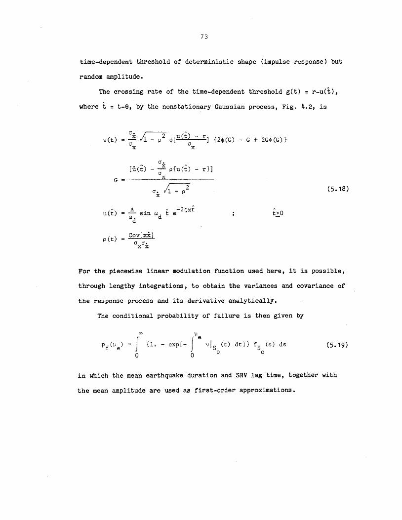
73
time-dependent threshold of deterministic shape (impulse response) but
random amplitude.
The crossing rate of the time-dependent threshold get) = r-u(t),
where t = t-9, by the nonstationary Gaussian process, Fig. 4.2, is
vet)
G
u(t)
p (t)
cr. =~
o x
0.
[u(t) x .....
- - p{u(t) 0 x
h 2 cr. - p x
A -2l,;wt = - sin w t e wd d
Cov[xx] cr o-x x
- r}]
(5.18)
t>O
For the piecewise linear modulation function used here, it is possible,
through lengthy integrations, to obtain the variances and covariance of
the response process and its derivative analytically.
The conditional probability of failure is then given by
CD
f {l. - exp[
o vis (t) dt]} fS (s) ds
o 0
(5.19)
in which the mean earthquake duration and SRV lag time, together with
the mean amplitude are used as first-order approximations.
The probabilities of lifetime maximum combined earthquake and SRV
response are compared in Fig. 5.10 for independent processes and for the
correlated processes. The exceedance probability increases
significantly due to the clustering effects. When both the intensity
and the occurrence times are correlated among load processes, the effect
may produce very much higher failure probabilities at high thresholds.
5.5 Conclusions
We have shown that the load coincidence method is well suited for
the treatment of correlated load processes of the intermittent
continuous type. Results of the non-exceedence probability of
combinations of these processes show similar trends to those found for
static Poisson pulse processes. Serious consequences may arise if
certain correlated effects are neglected in a design, the most important
ones being those due to intensity dependence between loads and also
occurrence clustering between loads.
75
CHAPTER 6
APPLICATION TO STRUCTURAL CODES
6.1 Introduction
6.1.1 Code Formats and Load Combinations
There is agreement amongst a growing number of engineers that
because of the random nature of loads and the scatter in the data of
material strengths, a probabilistic treatment provides a consistent
means whereby new structural codes may be developed. The trend is to
propose a limit states design methodology with load and resistance
factors provided to ensure a specified level of component reliability.
The main reason for this proposal is that a code should account for all
design situations including different types and numbers of loads,
geographical location, intended structural use, and different materials
and this is best accomplished by a number of factors rather than by one
global factor.
The selected formats in two codes are shown here as examples of
partial factor limit states checking equations. The designer is given a
number of load combinations (checking equations) together with the load
factors and characteristic values of the loads. These loads are
substituted, in turn, into the load combination equations and the most
76
severe load combination is the one that governs the design.
The National Building Code of Canada (NBCC) has adopted the format
(6. ,)
where D,L,Q,T are the dead, live, wind or earthquake, and deformation
loads respectively. The O! are the load factors, (/>. is the resistance
factor, Y the importance factor (usually = 1.0), and ¢ is the
combination factor.
1.0 for one load 0.7 for two loads 0.6 for three loads
The proposed format for the Load and Resistance Factor Design of
steel structures in the U.S.A. is;
(6.2)
where the "Yare the load factors, ~ is the dead load, Qi is the
maximum lifetime value of one of the variable loads and the Qj
are the
arbitrary pOint in time values of the other variable loads.
Both of these formats recognize the fact that when loads which vary
with time act on a structure, it 1s extremely improbable that their
maximum values will occur simultaneously.
When the nominal values of the loads are obtained from the
statistics of the maxima it is necessary to apply a load combination
factor to reduce the combined load. This is what is done 1n the NBCC
wi th the faotor ~.
77
The approach taken by the developers of the LRFD specifications is
to make use of Turkstra's rule (section 4.5.3) (Turkstra, 1970).
Combination of the loads requires summation of the maximum value of one
load with the arbitrary point in time value of the other loads. In the
actual design process only the characteristic (usually a percentile)
values of the maxima will be used so that the load factor on a load
which should take on its point in time value in a combination will be
less than 1.0 while that on a load taking its maximum value will be
greater than one.
These two methods of dealing wih the combination of loads which
vary with time are simplified methods thought necessary for use in
structural codes due to the way in which design loads are specified in
today's codes. In the first case the designer actually applies the
reduction factor, whereas in the second Turkstra's rule is used by the
code-writing committee and the designer merely applies the partial load
factor specified.
An extensive study was undertaken by Ellingwood, Galambos,
MacGregor and Cornell (1980) in developing the latest code reqUirements
for minimum loads in buildings (ANSI A58.1-1982). We remark here on
some observations and questions raised in that study in light of the
methodology developed herein and the findings obtained so far.
78
6.1.2 Code Calibration
The purpose of code calibration (Siu, Parimi and Lind, 1975) could
be described as avoiding the introduction of levels of reliability less
than the least aoceptable in current practice.
This requires the evaluation, through probabilistic modeling and
analysis, of the current implied reliability (termed notional
reliability because it is not absolute) present in the codes.
Ellingwood, et al., obtained these values, for different load
combinations, in the form of reliability indices.
It was found that the reliability indices implied by current design
equations for combinations including earthquake loads were lower than
those including wind loads, which in turn were lower than those
including just live loads. It was decided to retain this practice in
the new specifications.
6.1.3 Adolescence
We should note that, although probabilistic methods have been used
throughout the development of the new specifications (ANSI A58), in the
end, compromises were deemed necessary to ensure a smooth transition for
engineers and for the safety of the structures.
This may, in part, be put down to the fact that, though structural
reliability theory has been termed a healthy adolescent, (Cornell,
1982), it still is in its adolescence. The new specifications are a
natural step along the way to becoming an adult.

79
We believe that the load coincidence method of combining time
varying loads will provide understanding and a tool for growth.
6.2 Code Optimization
The objective of a design is twofold; (1) to achieve an acceptable
level of safety, and (2) to do so at the least possible cost. Ravindra
and Lind (1973) wrote that "structural code optimization is the search
for a rational balance between society's investment in structures and
the reliability achieved." Ideally, this can be done by considering
costs associated with construction and the consequence of failure, with
the design variables being chosen such that an optimum can be reached in
terms of risk-benefit trade-off.
Optimization over the whole data (design) space is an enormous
task. One of the major difficulties is, of course, putting a value on
the loss of a human life due to structural failure. At the next level,
a design can be based on an acceptable level of probability of failure
(limit state being exceeded)~ For example, what has been attempted by
the ANSI study is such a risk-based code without direct consideration of
cost. However, an allowable risk of failure can be satisfied by an
infinite number of designs, but the desired one is the one which is an
optimum in terms of yielding minimum cost. Calibration with present
practice may put some constraint on cost and therefore may not be an
optimum.
80
The present format in structural codes (Section 6.1.1) obviously
has limitations in achieving the target reliability in all the designs
because one equation attempts to take account of a wide range of
structural types and loads. For a given design situation (structure
type, geographic area) one of the combination equations is meant to
dictate what resistance is required. That is, knowing the loading
situation one should be able to recognize which will be the determining
equation for the design. This combination equation carries with it an
implied reliability which the component should attain. This certainly
is true when one combination clearly dominates the others, e.g., wind is
the major force to consider and there is little earthquake risk.
However, when two combinations give similar results (e.g., D+L+W
and D+L+E) the implied reliability is undefined in the current procedure
and is obviously lower than under any particular load combination. We
say this because one combination gives a value of 2.5 for the
reliability index while the other gives a value of 1.75, yet the design
is the same for both.
No combination including both wind and earthquake appears in the
specifications because, though both may occur at one site during the 50
year design life, they have small likelihood of occurring simultaneously
at combined values exceeding the maximum of one load (Turkstra and
Madsen 1980). However, the exclusion of the one load is necessarily an
unconservative step, most significant when the two combinations are
similar in value.
81
This is demonstrated by making use of the load coincidence method
in the design of a member and the evaluation of the consequent
reliability for different combinations. The procedure first requires
the stochastic process modeling ,of the loads (D,L,W,E) at a given
location so that the extreme value distributions match those given in
the ANSI study (Ellingwood, et al., 1980) for the design life of 50
years.
In reality, of course, a structure (member) will be subjected to
all the load processes over the design life, rather than a given code
specified load combination. The reliability of a member with given
resistance is therefore calculated for the total combined process using
the load coincidence method. To'obtain the best design which satisfies
the reliability constraint, a simple one dimensional search is utilized
until the minimum resistance is obtained. Having obtained the required
deSign, its reliability for different combinations of the loads is again
calculated using the load coincidence method.
Results of the reliability indices for the different combinations
are shown in Table 6.1 for different ratios of the varying loads (L,W,E)
to the dead load CD). The optimum (minimum) resistance, R, is also
given as a ratio of the dead load. The target reliability index for the
total load combination is 2.33 (failure probability = 0.01). The index
implied by each combination differs most from the target index when two
combinations show similar design requirements. This effect may be
serious for situations where many combinations of numerous loads are
prescribed, such as in the design of nuclear power plants.
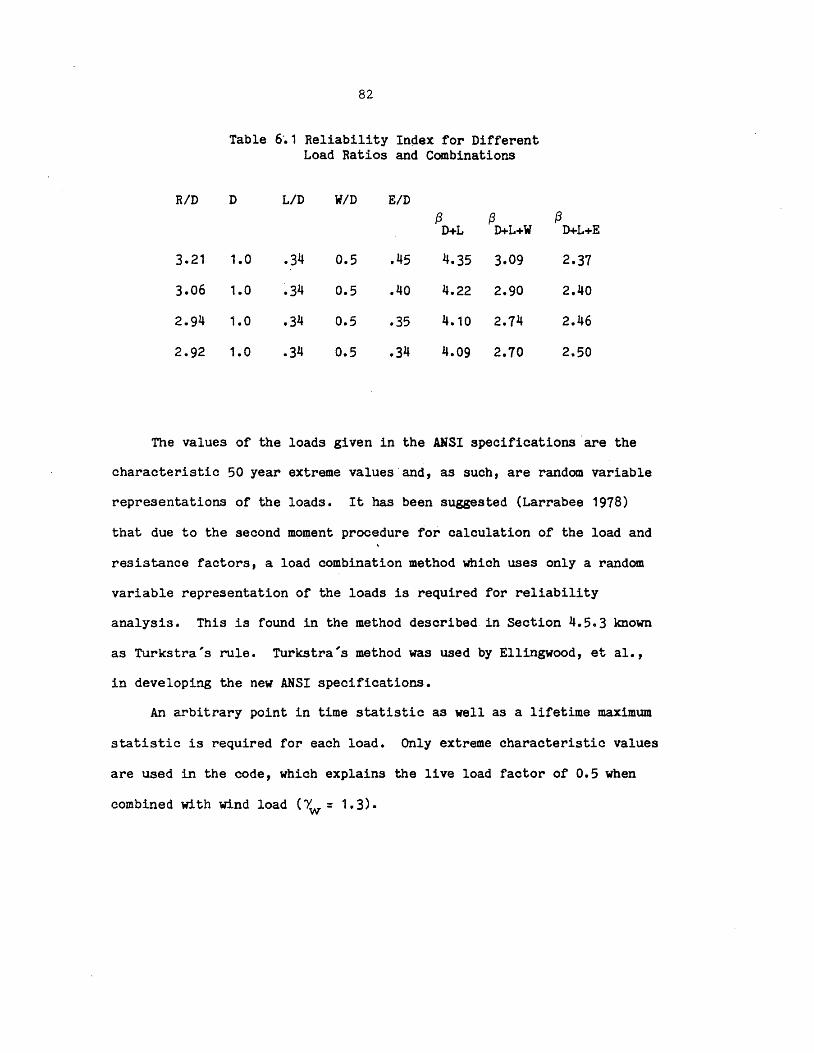
82
Table 6'.1 Reliability In~ex for Different Load Ratios and Combinations
RID D LID WID E/D {3 {3 {3
D+L D+L+W D+L+E
3.21 1.0 .34 0.5 .45 4.35 3.09 2.37
3.06 1.0 .34 0.5 .40 4.22 2.90 2.40
2.94 1.0 ,34 0.5 .35 4.10 2.74 2.46
2.92 1.0 .34 0.5 .34 4.09 2.70 2.50
The values of the loads given in the ANSI specifications "are the
characteristic 50 year extreme values "and, as such, are random variable
representations of the loads. It has been suggested (Larrabee 1978)
that due to the second moment procedure for calculation of the load and
resistance factors, a load combination method which uses only a random
variable representation of the loads is required for reliability
analysis, This is found in the method described in Section 4.5.3 known
as Turkstra's rule. Turkstra's method was used by Ellingwood, et al.,
in developing the new ANSI specifications.
An arbitrary point in time statistic as well as a lifetime maximum
statistic is required for each load. Only extreme characteristic values
are used in the code, which explains the live load factor of 0.5 when
combined with wind load (Y'w = 1.3).

83
However, as has been found in this study as well as in Wen (1980a),
Turkstra's rule yields unconservative results for the maximum in (O,t)
of the combined process and for certain load types and probability
levels this unconservatism can be quite serious. The load coincidence
method gives a more realistic treatment of the problem yet
computationally is still efficient. Therefore it can be used in the
formulation of a risk-based building code as exemplified in the
foregoing. This can be ~one so that the optimum resistance is obtained
for the given loads and desired reliability. Having obtained the
required reSistance, the load and resistance factors, consistent with
current code formats, can then be evaluated. These nominal loads are
taken from the distribution of the maxima in the 50 year design period.
Therefore, second moment methods (togeher with some full distribution
information) may be applied, using the extreme distributions of the
loads (as in ANSI) to calculate the load factors.
Summarizing: given a design life target reliability, the load
coincidence method enables the calculation of the required reliability
for any given combination of loads; and combined with a second moment
analysis, permits the computation of load factors which are more
internally consistent than the current formulation and yield a design of
prescribed reliability against all loads.
84
6.3 Choice of the Target Reliability
The discrepancies between the reliability indices implied by
current practice for combinations of dead and live loads, and those
including either wind or earthquake loads have been mentioned earlier.
The question is how are these differences to be interpreted and can we
tolerate such low reliability for members subjected ~o earthquakes?
The committee developing the new specifications decided to retain
these values of the reliability index for the new codes so as not to
upset present practice when insufficient data is available to suggest
radical changes. This seems to be the prudent thing to do right now.
However there are some pressing questions in light of this which do need
attention.
One statistic given to back up this decision is that buildings
appear to be surviving well thus far. It is true that successes are
documented but it should be pointed out that statistically speaking we
do not have sufficient experience with earthquake loads to back up the
statement.
It has been suggested that the computed reliability is an apparent
reliability due to mitigating effects which do not occur due to live
loads, e.g., live loads act directly on the members, whereas the lateral
forces of earthquake and wind act on the whole structure. The way the
analysis was performed in the study by the NBS would not allow these
differences to affect the final result unless the statistics of the
earthquake forces were erroneous. The study took no account of how the
load was applied, but considered only a number of ratios of the load
effects.
85
Another suggested reason for the lower reliability is the use of
the load reduction factor of 0.75 when combining D+L+W or D+L+E
(Galambos, et al., refer to this as the one third increase in allowable
stress). The implication is that the resulting value of the load is an
unconservative estimate of the maximum of the combined loads, and the
~actor would have to be increased. To demonstrate that this is not so,
we compare the failure probability implied by using the LRF and the load
coincidence methods. The loads considered are the combination of dead,
live and wind. The extreme (50 year maximum) statistics are those used
in the ANSI study~ The stochastic process models are computed such that
the extreme values match those of the 50 year maximum used above. The'
mean occupancy for the live load'process is 8 years and the m~an
occurrence rate of significant wind is 10 per year. The result is
plotted in Fig. 6Q1 showing the conservative use of the LRF of 0.75.
Numerical integration was used with full distribution information, for
the computation of the probabilities. The SRSS rule for three loads
gives similar results to the load reduction factor procedure with a
factor of about 0.6. A factor of 0.75 will therefore always be more
conservative than the SRSS. The conservatism depends on the mean
occurrence rate A of each of the loads when the conditional failure
probability given occurrence is independent of the duration (i.e.,
static loads). For dynamic loads the LRF is conservative for all A at
medium and large failure probabilities.
86
It is important that research is continued to evaluate the accuracy
of the earthquake statistics and the reliability calculated in the ANSI
study before an optimizing risk-benefit study can be initiated.
A quite plausible explanation for tne reduced reliability ia our
willingness to accept damage due to rare natural events such as extreme
winds and earthquakes. We are not, however, willing. to accept the same
kind of damage due only to some excessive live load. This is evidenced
by the public reaotion to failures due to both of these causes.
87
CHAPTER 7
SUMMARY AND CONCLUSIONS
7.1 Summary
The problem of evaluating the probability that a structure becomes
unsafe under a combination of loads, over a given time period, is
addressed. The loads are modeled by stochastic pulse processes,
characterized by the mean occurrence rate and the mean duration of the
pulses and by a description of the variation of the load within a pulse.
Static loads (effects) are represented by pulses with some specified
shape. Dynamic loads are modeled by a zero-mean Gaussian process,
superimposed on a rectangular static component for those loads with
non-zero mean.
Exact solutions to the load combination problem are, in general,
difficult rare and an upper bound solution given by the mean number of
crossings in (O,t) is usually sought.
The load coincidence method (Wen 1977) is extended to problems with
both nonlinear limit states and to dynamic responses, including the case
of correlated dynamic responses.
88
Linearizing a nonlinear limit state is a commOn way of obtaining
reliability estimates for time invariant problems. This same technique
is investigated for time-varying combination porblems, with emphasis on
selecting the linearization pOint.
The load coincidence method is formulated also for dynamic
combinations and compared with other methods, namely the upcrossing rate
methods. Use of simpler rules (SRSS and Turkstra) for load combination
is also compared with the results from the more complete stochastic
process models.
Correlated effects amongst dynamic loads are examined to see how
results differ from correlated static loads, and to demonstrate which
types of load dependencies are most important, i.e., affect the
exceedance probabilities the most.
Application of the load coincidence" method to code development is
briefly discussed.
7.2 Conclusions
Conclusions from this study may be summarized as follows;
1. There is a uniquely optimum point at which a nonlinear limit
state should be linearized for approximate evaluation of the
crossing rate out of the domain. The point is the stationary
point of the mean crossing rate out of the tangent hyperplane,
and is found by a suitable nonlinear programming algorithm.
For a concave safe domain the point is a local minimum, whereas
89
for a convex safe domain it is a local maximum.
2. The load coincidence method may be easily applied to the case
of a nonlinear limit state. When the conditional failure
probabilities can be obtained exactly the results are very good
especially for sparse processes, i.e, they give close,
conservative estimates of the overall failure probability.
When the exact conditional failure probabilities are
unobtainable, approximate convolution by the Rackwitz/Fiessler
algorithm may yield sufficiently accurate results. However,
depending on the shape of the domain and the probability
distributions of the basic variables, it is not always possible
to say whether the estimate is conservative or not.
3. New techniques (e.g., the multiple checking point approach;
polynomial fitting) for evaluating the probability content of a
nonlinear domain can be easily incorporated in the load
coincidence method.
4. The "crossing rate" methods, which use the crossing rate of the
dynamically fluctuating process to calculate the expected
number of crossings in (O,t), tend to be overly conservative in
the evaluation of the failure probability over the prescribed
design life, particularly for long load duration, short period
structures, and low to medium failure thresholds.

90
5. Use of the conservative "Poiss~n approximation", for the
conditional first passage probability given occurrence or
coincidence of a load, does not have significant effect on the
overall lifetime failure pr~bability.
6. Use of the mean duration in the computation of the conditional
failure probability is a reasonable first order approximation
and greatly reduoes computation time and effort. Its accuracy
has been carefully examined by analysis as well as Monte Carlo
Simulation and found to be very good.
7. The load combination rules (SRSS, LRF, Turkstra) applied in
codes and code development are not consistent in their
estimation of the combined maximum load for intermittent
oontinuous processes. The sass is affected more by the
structural parameters and is generally conservative for the
high and medium risk levels, while Turkstra's rule is always
unconservatlve and is affected more by the load process
characteristics ( A , SJ. ).
8. The dynamic process model used is suited for modeling
correlated effects both within and between loads. The analysis
is more involved than for correlated static loads but the
trends in the results, for the non-exceedance probability of
combined loads, are similar.

91
9. The most significant correlation effects are seen for loads
which have intensity dependence between processes and for
occurrence clustering between processes. At medium to high
thresholds these effects are especially important, and a
combination of the two could be even more serious.
10. The present practice of neglecting certain loads in combination
equations because of the small probability of their
simultaneous occurrence with other loads in the combination, is
unconservative. However, the unconservatism is only
significant when the two loads are equally important in causing
load effects on the structure or when a large number of loads
needs to be considered.
11. The load coincidence method can be well utilized in the
development of probability based structural codes, by obtaining
an optimum design for a given target reliability constraint
under a set of real loads. Reliability indices may then be
calculated for any given combination of loads and advanced
second moment methods used to obtain load and resistance
factors.
12. The questions arising from the difference in the reliability of
members designed only for live loads and those designed for a
combination of live and earthquake loads seems to imply that
more research is needed on the accuracy of the earthquake data
92
before we can be sure that present practice is as it appears.
13. The load coincidence formulation has proved to be a relatively
simple, versatile and accurate method for the evaluation of the
failure probability of a structure under the combined action of
a number of time varying loads.

93
FIGURES
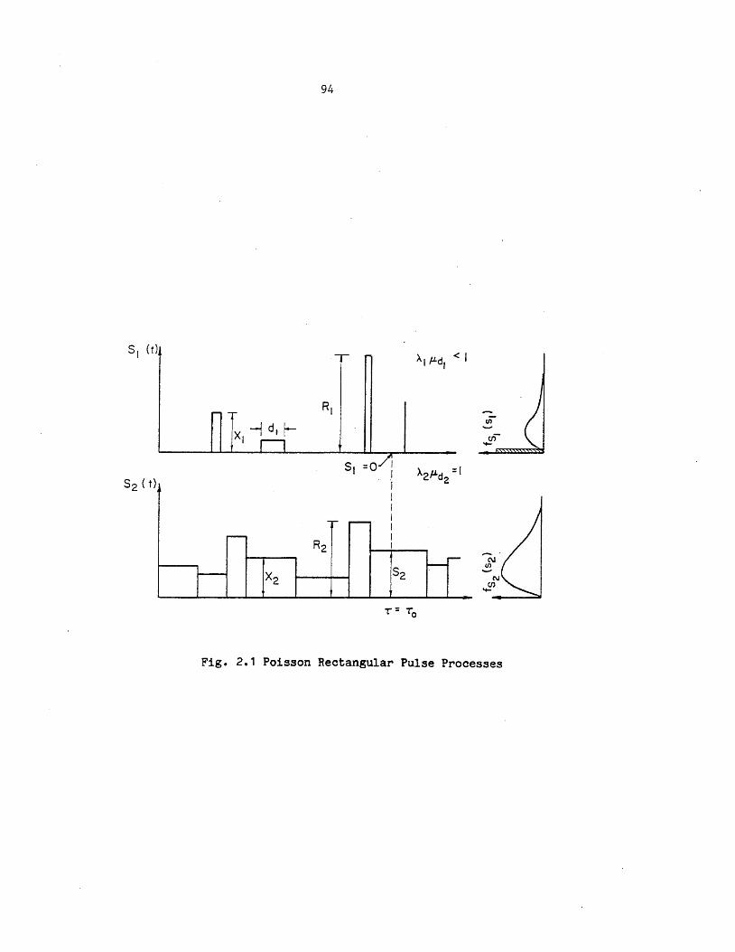
94
-r-
I"""" -RI
X -1 d t f-I 11
-.-
......-R2
r- X2
- . ./1
I I t
r0- I I I
52
A I ,ud,
-
<I
r--
N en ~
Fig. 2.1 Poisson Rectangular Pulse Processes
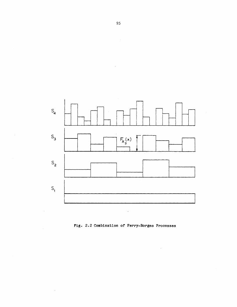
95
...-
~ (x) 3 1
I I
Fig. 2.2 Combination of Ferry-Borges Processes
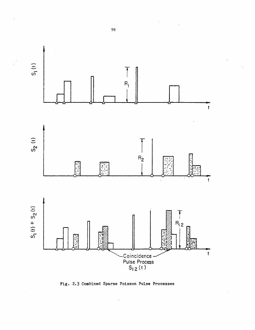
--
---C\J en
C\J Cf)
+ -..=. Cf)
:.:-: ... .. : ..
.. :~. "." .,.1
.......
. ?~:~: \: 1'-: .._:- • I •
96
T
T
Coincidence Pulse Process
512 (t )
. ~ .... "''' , ~ ~ ~".~,:".-. , .
J • ; ...
Fig. 2.3 Combined Sparse Poisson Pulse Processes
t
t
T
t
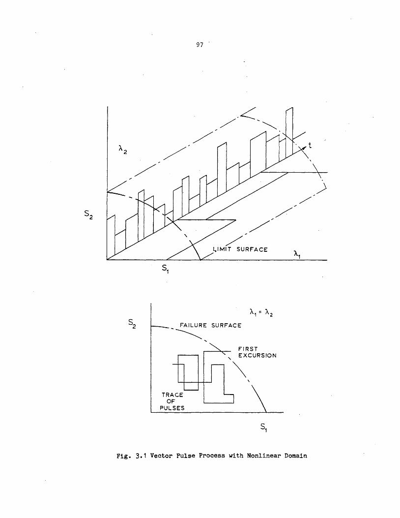
97 .
, /
L,IMIT SURFACE
FAILURE SURFACE
~
TRACE OF
PULSES
FIRST " EXCURSION
'\ ,
Fig. 3.1 Vector Pulse Process with Nonlinear Domain
t
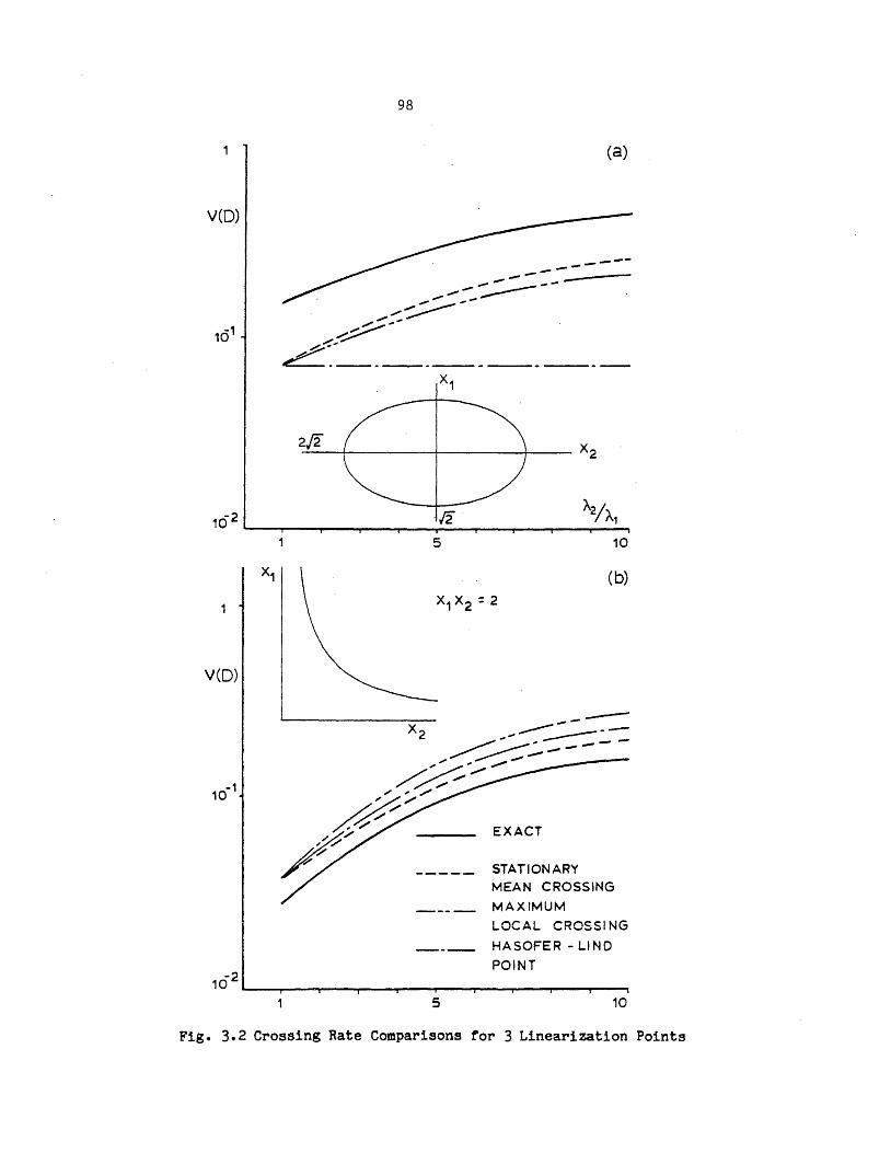
V(O)
102
x1
V(O)
98
(a)
... --------- .~--.,...""'" ----~
....... - --------_ ...... --- ...... /~
/ ~~ -
~ ./:.~ ... L ___________ _
2/2
><1
X2
-./2 "'A2/A1
5 10
(b)
x1 x2 = 2
5
EXACT
STATIONARY MEAN CROSSING
MAXIMUM
LOCAL CROSSI NG
HASOFER - LI ND
POINT
10
Fig. 3.2 Crossing Rate Comparisons for 3 Linearization Points
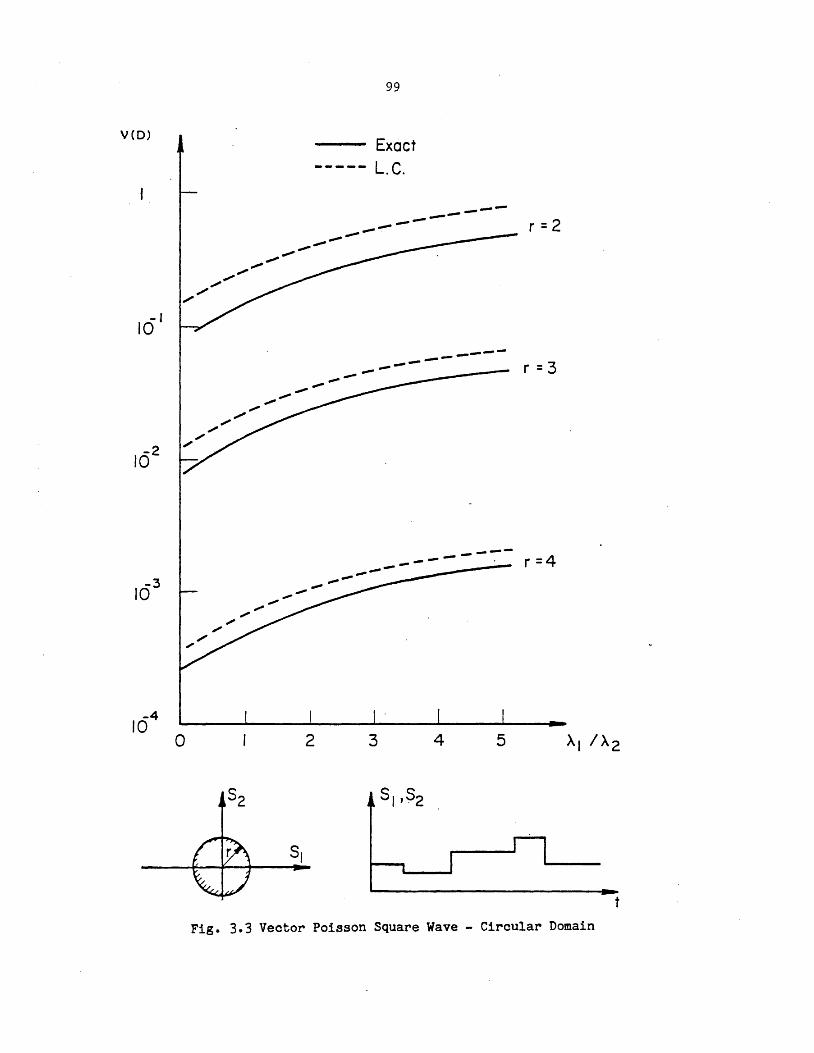
V(O)
o 2
99
Exact L.C.
r=2
r = 3
_ .... ----- r=4
3 4 5
Fig. 3.3 Vector Poisson Square Wave - Circular Domain
t
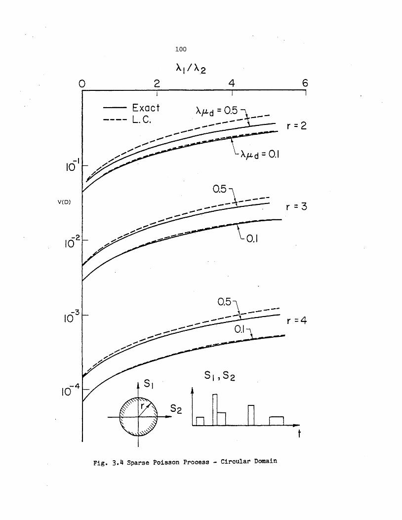
o
V(D)
2
Exact ---- L C . .
100
4
AfLd = 0.5
0.5
0.5
6
r = 2
AfLd = 0.1
---r=3
0.1
r=4
D D ... t
Fig. 3.4 Sparse Poisson Process - Circular Domain
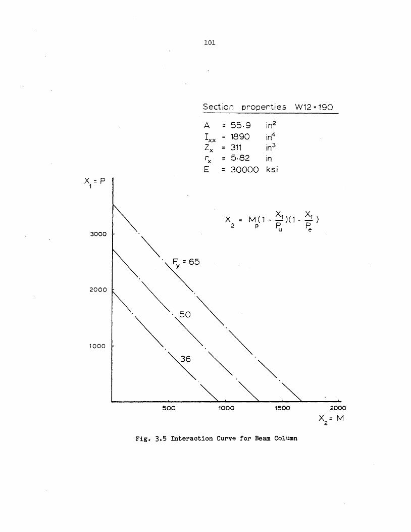
3000
2000
1000
101
x = M (1 - X1) (1 _ X1 )
2 p ~ ~
500 1000 1500
Fig. 3.5 Interaction Curve for Beam Column
2000
X=M 2
102
Exact· crossing rate "-
10 '\ ----- Load coinc idence
'\ '\
'\ (1) A =10 u1 =0.1
\ 1 \
\ A=20 U =.05 \ 2. 2
\ ( 2) i\ =10 u =.01
\ \ 1 1 \
\ A=20 U =.025 \ 2. 2.
\ , \ (3) i\ = 10 u1 =.01 1
~ \ 4
~ ~ ~
\: '\ ~ " =10 U2.=.01 ~ ~
2. '\
V(D) '\ ~ \
'\ '\ \ '\ \ \
" \ \' '\ \ \
'\ \
\ \ -1 \
\ .~ 10 \
\ \ ~
\ \ ~ \ \ '\
\ \ '\
\ '\ \ \
\ \ \ \ \ \ 1 \ \ \ \ \ \ \
-2 \ \ 10 \ \
\ \ \ \ 2
\ \
\ \
\
-31 \ "'" , ...)
10 30 40 50 60 70
Fig. 3.6 Crossing Rates for Beam Column Fy
103
0, x Occurrence Time Point Process
x(t), SXX(W)
I .. ..I Fig. 4.1 Intermittent Continuous Process
lOL~
1.0
d MODULATOR FUNCTION
e
Fig. 4.2 Combined Nonstationary Processes
105
THRESHOLD r
3 4 5 6 7
, "- '\ " " \
"-
'\ -1 ' \
10 '\ ~
/DIRECT \\\ \ ,
-2 \'\ 10 ' \ \\"
\ , \'\
163
CONDITIONV\.\,
\ ~ \\ -4 \'\ 10
\ \ LOAD COINCIDENCE -\ '\
-5 \ 10 \\
\ ~
\\ -6
\ , 10 \
\
Fig. 4.3 Point Crossing Method - Direct and Conditional
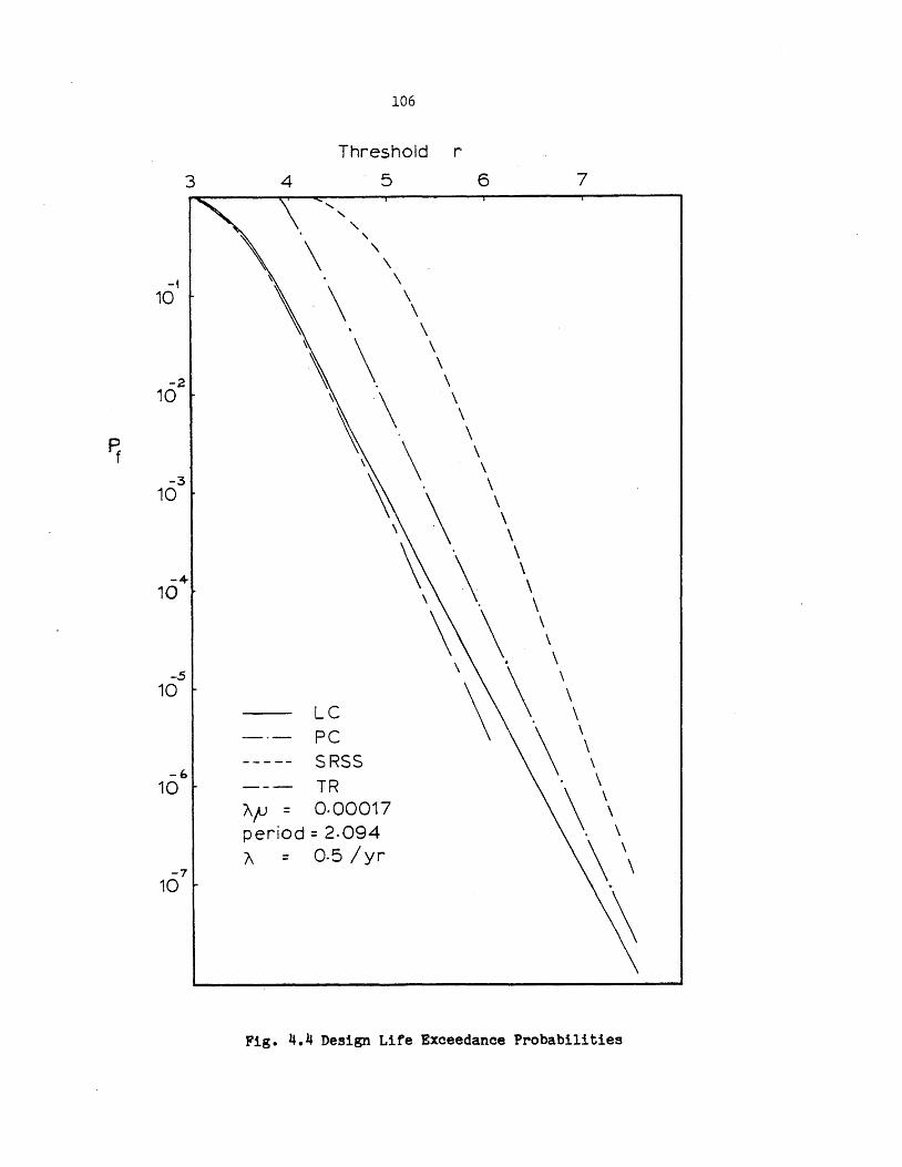
106
Threshold r
3 4 5 6 7 "-
" "-
\ ,
\ '\ \
-1 ~ \ 10 \ \ \
\ \
~ \ \
\ \ -2 \
10 ~\ \ \
~ \ . \
\ \ \ \
-3 ,. \ 10 \ \\ \
\
~ . \ \
-4 \\ \ 10 \
'\ \ \ \
\ . \
-5 \ \. \ 10 LC
-.- PC \\ --- -- SRSS -b
10 --- TR \
"fJ = 0·00017 \ \ period = 2.094 . \
" = 0.5/yr \\ -7 10 .
\
Fig. 4.4 Design Life Exceedance Probabilities
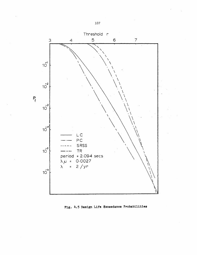
107
Threshold r
3 4 5 6 7
"-, '\. . \
\\ -1 10 \ \
\\ -2 \ \\ 10 \ . \
~ \ \\ .\
-3
\ \\ 10
\ . \
\ \\ -4- . \
10 \ \\ LC \ _.- PC . \
\ --- -- SRSS -5
\ \
10 --- TR \ period = 2.094 sees '\ I\fJ = 0·0027
1\ = 2/yr -0 \"
10 \~ ~
Fig. 4.5 Design Life Exoeedance Probabilities
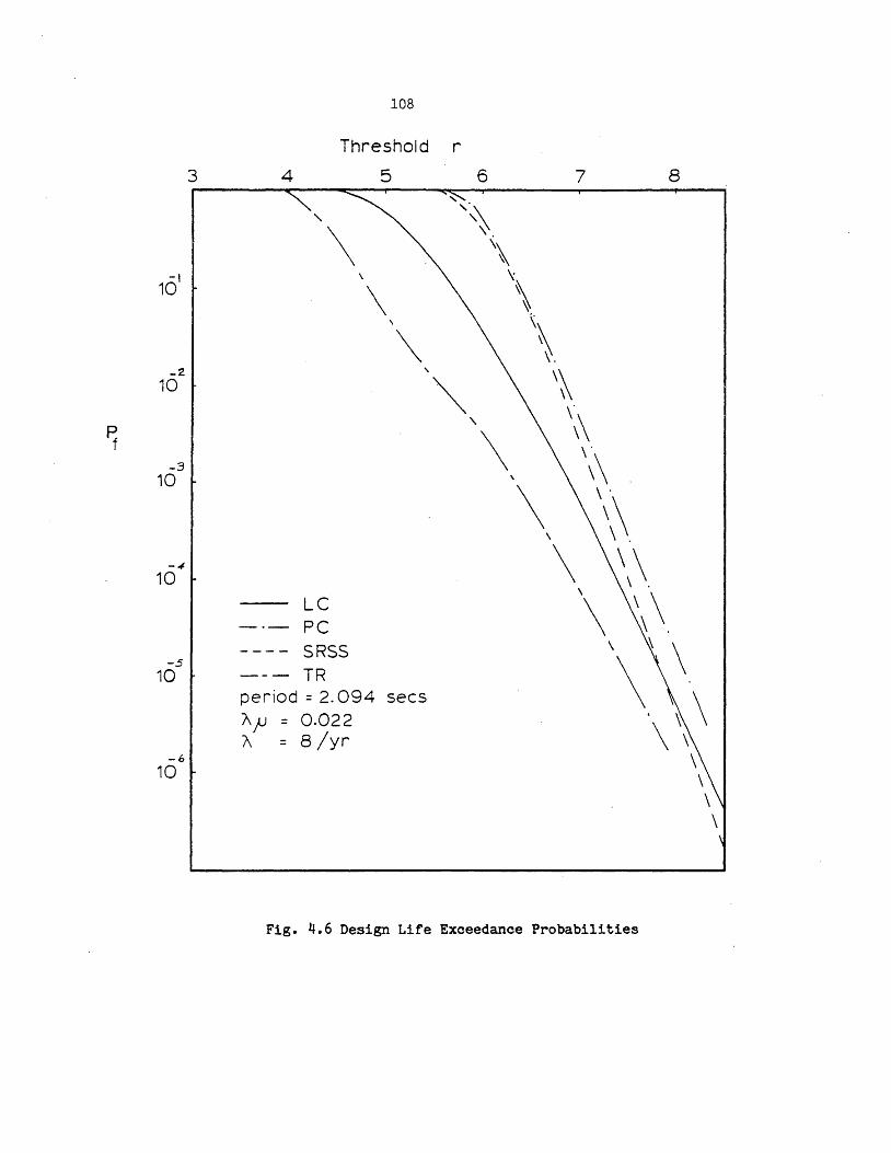
108
Threshold r
3 4 5 6 7 8 "-
" '~\ \ "\
-I \ \' 10 \ \
\
\ \ \. -2
, '\ 10 ~ \\ " ~ \ \'
-3 \\ 10
\ \ .
\\ \ \ ,
-.f. \ \\ 10 \ .
\
\ \ LC \ -0- PC ~ . --- - SRSS \ ~
\ -5
\ 10 --- TR period = 2.094 sees
. ~ \ "jJ = 0.022 A = 8 /yr \ \
-6 \ 10 \
\ \
Fig. 4.6 Design Life Exceedance Probabilities
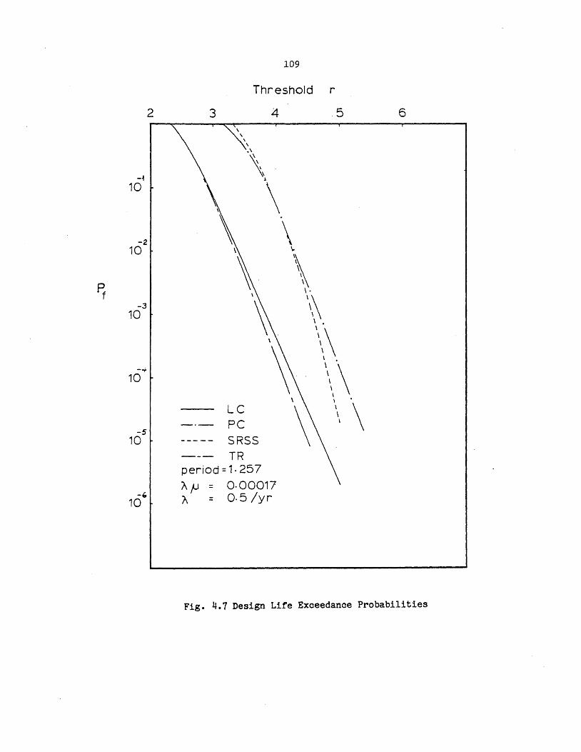
109
Threshold r
2 3 4 5 6 \
\ , \ .\
-~ \
l
10 \ -2 \ \
10 \.
~ \ '\ \ .
-3
~ \\ 10 \ .
\\ ~.
\ . -.... \\ 10
\ \
LC
\ \ \ \ _.- PC \
-5 10 ----- SRSS
--- TR period = 1· 257
"fJ = 0·00017 -, 0.5/yr 10 " =
Fig. 4.7 Design Life Exceedance Probabilities
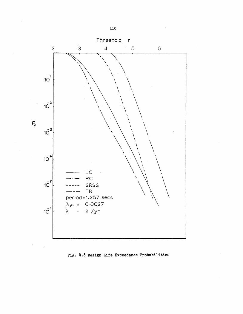
110
Threshold r
2 3 4 5 6
" , " \
\ \ \
\
-1 \ 10 \ 0\ \
\ \ \
\ \ -2 \
10 \ \
\ \ \ \ \
~ \
\ \ -3 \
10 \
\ \ \
\ \ \
\ \ 104- \
\
\ \ \
LC \ \ _.- PC \ \
\ -5 \ \ \ 10 ----- SRSS
--- TR period:1.257 sees \
"fJ = 0·0027 -6
10 " = 2 /yr
Fig. 4.8 Design Life Exceedance Probabilities
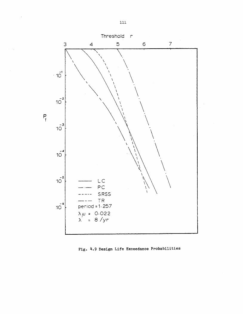
~
3
-1 ·10
-2 10
-3 10
--' 10
-5 10
-6 10
\
III
Threshold r
4 5 6 ,
\ \
\ \ \ \ \
\
\ \ \
\ \
~ \
\ \ \
\ \
\ \\ \ \ \ \
\\ \ \
\~ ~
LC _.- PC ----- SRSS --- TR period = 1· 257
"fJ = 0.022 " : 8 /yr
\
\
~
7
\
\ \ \
Fig. 4.9 Design Life Exceedance Probabilities
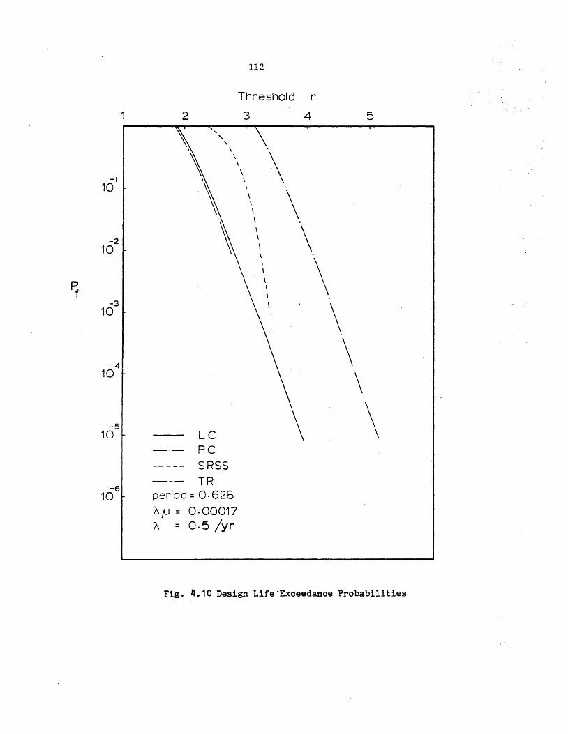
112
Threshold r
1 2 3 4 5
" " '\
\
\ \
\ \
\ -I \
10 \ \
\ \ \
\ \
\ \ \ -2 \
10 \ \ \
\ \
~ \ I
\ -3 \
\ 10
-4 \ 10
\ -5 \ 10 LC
-'- PC ----- SRSS
--- TR -6
period = O· 628 10
"fJ = 0·00017
" = 0.5/yr
Fig. 4.10 Design Life " Exceedance Probabilities
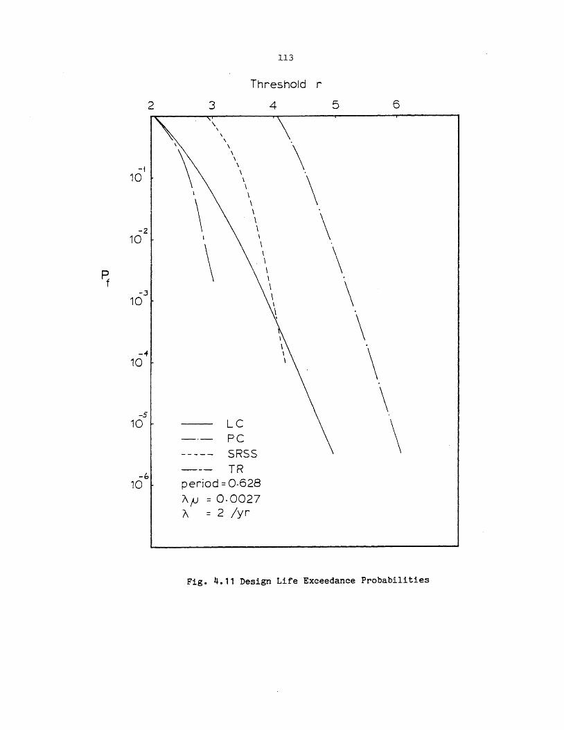
113
Threshold r
2 3 4 5 6
\ \
\ \
\
\ \ \
\
-i \
10 \ \
\ \ \
\ \ \
\ \ -2 \
10 \
\ \ \ \ \
~ \ \
-,3 \ \ 10 \
\
\
\ \ \
\ -4f , 10 \
-5 \
10 LC \ _0- PC ----- SRSS
--- TR -b
10 period = 0·628
AfJ = 0.0027 A = 2 /yr
Fig. 4.11 Design Life Exceedance Probabilities
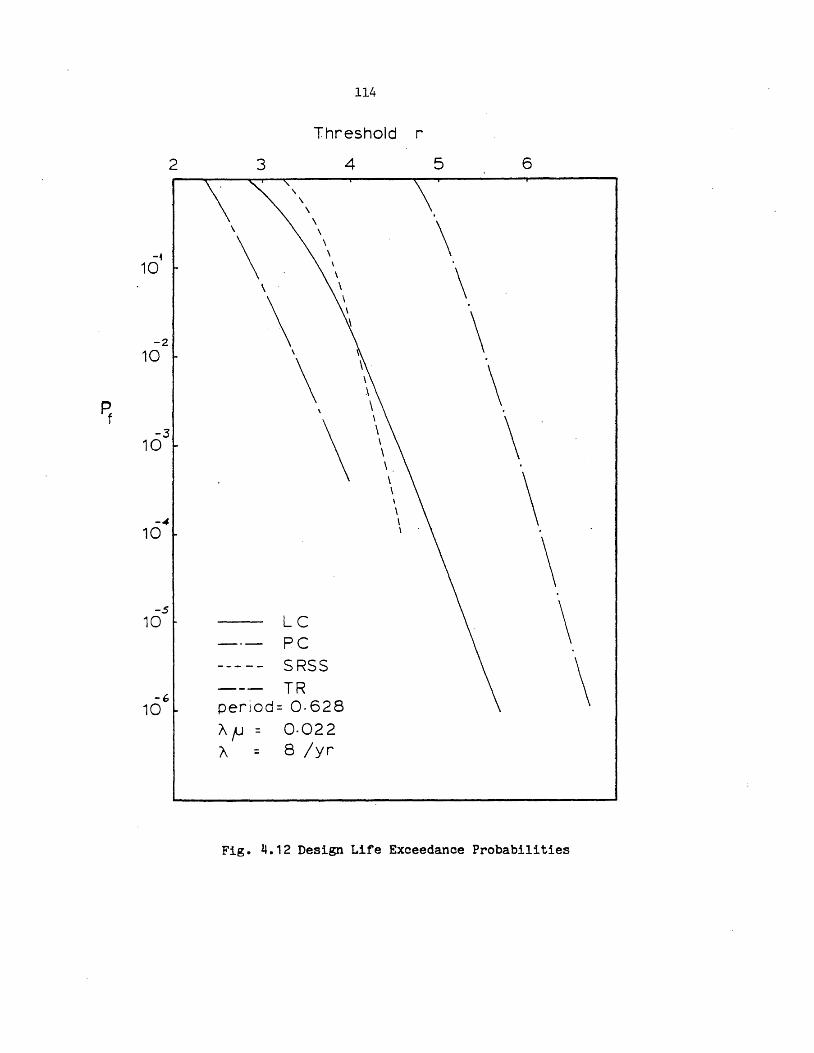
114
Threshold r
2 3 4 5 6
\ , \
\
\ \ \
\ \
-1 \
10 \
\ \ \ \
\ \
\ ~
-2 10 ~
\ \ .
\ \
.\
~ \
\ \
\ -3 \ 10 \
\ \ \ \ \
\
\ -4- \
10 \
\ -5 \ 10 LC
_.- PC --- -- SRSS \ --- TR
-6 period= 0·628 10
"fJ = 0·022
" = 8 /yr
Fig. 4.12 Design Life Exceedance Probabilities
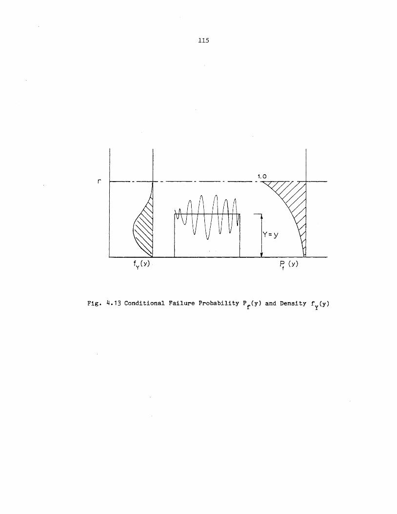
115
1.0 r
Y=y
~ (y)
Fige 4.13 Conditional Failure Probability Prey) and Density fy(Y)
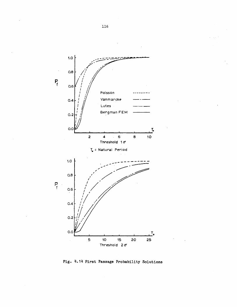
116
1.0 -- .- -- - - -- -, .. ..::--- -, .. / ,
;'
, I , 0.8 It' ;/ , I
~ .I I
" I 0.6 I j I
I Poisson --------I
" , I Vanmarcke ----0.4 I
# I Lutes -----, , Bergman FEM 0.2 I
I I
2 4 - 6- 8 10
Threshold 1 a'
T. = Natural Period
1.0 --- -----------,,' ,~ ~ 0.8 /" / .......
/ ' ,/ 0.6 :' / ~ ••
I I //
04 // /
·t;! 0.2 i/,
" , I I
I
0.0 To
5 10 15 20 25 Threshold 2 (1'
Fig. 4.14 First Passage Probability Solutions
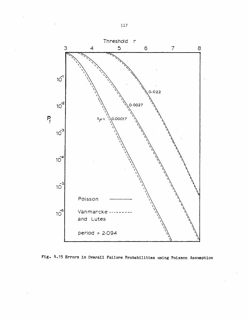
117
Threshold r
3 4 5 6 7 8 .... ,
" " .... .... .... .....: .... "
.... .... .... ....
.... \
" .... , .... " \ .... " \ ,
'\ -1 \ ....
\ " 10 \ \ \ \ \ \ ,
\ ~ \ \ \ '\ 0.022 ,
\
'\ \ '\
\ \
102 \ \ 0·0027 \ \ \ \ '\
\ \ " \
~ "'f1 = \ \ 0·00017
\ \ \ \ \ '\ '\
-3 '\ '\
10 \ '\ \ '\ \ \
'\ \ \ \ ,
\ ,
\ \ ~
\ '\l \ \
\ \ \
104 \ '\
\ '\ \ \
\ \ ~
\ \ ~ \
\ '\ \ \
\ \:
-5 \ \
10 '\ , \ \
Poisson \ \
~
\ '\
\ '\ -6 Vanmarcke --------- \ 10 \ ,
and Lutes \ \
\ ~
\ \ \
\ '\ \ period = 2·094 \ \
~
Fig. 4.15 Errors in Overall Failure Probabilities using Poisson Assumption
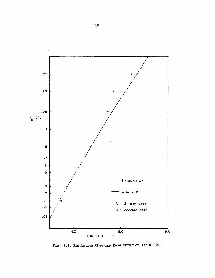
.99
.98
.95
.9
.8
.7
.6
.5
.4
.3
.2
.1
.05
.01
0
0
4.0
118
o
o
o
o
o SIMULATION
-- ANALYSIS
THRESHOLD r
A = 2 p~r y~ar
~ = 0.00137 y~ar
5.0
Fig. 4.16 Simulation Checking Mean Duration Assumption
6.0
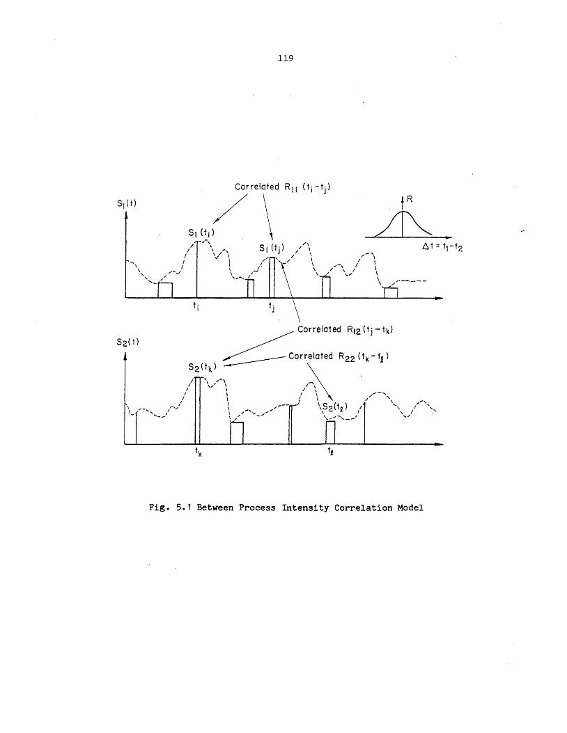
119
Correlated RII (t· - t· ) I . j
SI( t) / \ A S, OJ) .. /
.... .,-, S I (tj)
..... , D. t = t,-t2 \ .I \ I \ ".,
/ \ I \/ \ ..... -.... I ,,' .1/ \ I \ .....
I I \ .... -, I \ \ I ,. \ /,./ \ ,.J \ .- .I \ I \ , \ .- \ .... " \
"- , " ' ... -... / \ '- \ "
,,------
Fig. 5.1 Between Process Intensity Correlation Model
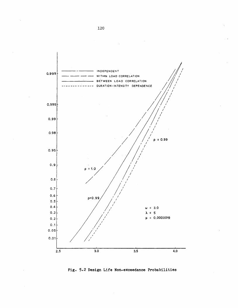
0.999
0.995
0.99
0.98
0.95
0.9
0.8
0.7
0.6
0.5
0.4
0.3
0.2
0.1
0.05
0.01
2.5
120
INDEPENDENT
WITHIN LOAD CORRELATION
BETWEEN LOAD CORRELATION
DURATION -INTENSITY DEPENDEN.CE
3.0 3.5
w = 3.0
A = 5
Il = 0.0000019
4.0
Fig. 5.2 Design Life Non-exceedance Probabilities
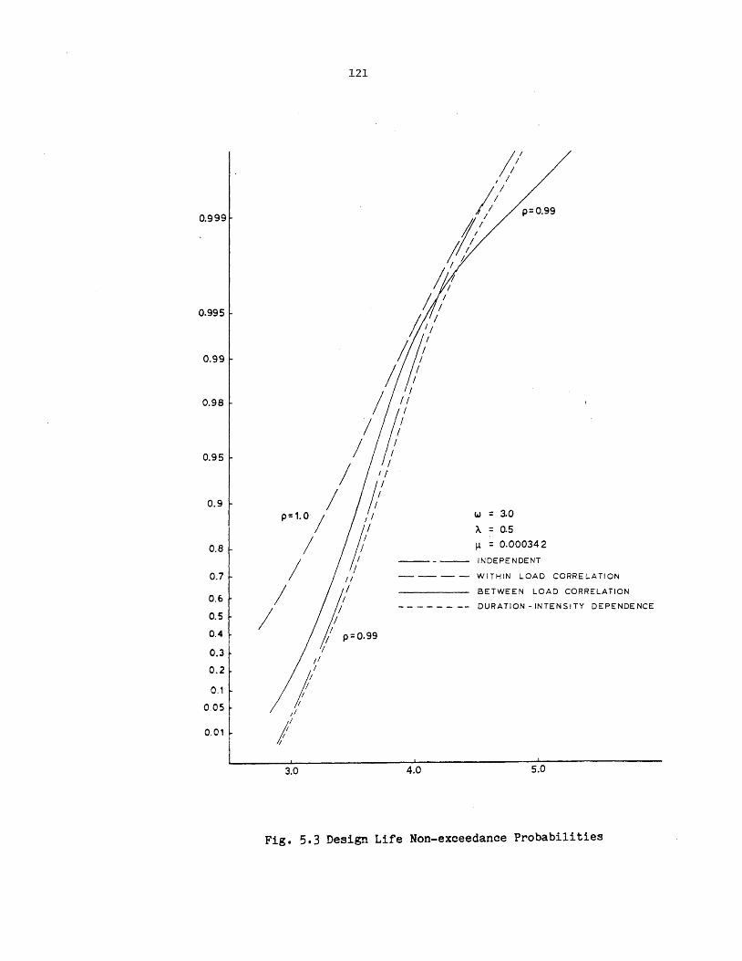
0.999
0.995
0.99
0.98
0.95
0.9
0.8
0.7
O.b
0.5
0.4
0.3
0.2
0.1
0.05
0.01
121
3.0 4.0
w = 3.0
A = 0.5
~ = 0.000342
INDEPENDENT
WITHIN LOAD CORRELATION
BETWEE N LOAD CORRELATION
DURATION -INTENSITY DEPENDENCE
5.0
Fig. 5.3 Design Life Non-exceedance Probabilities
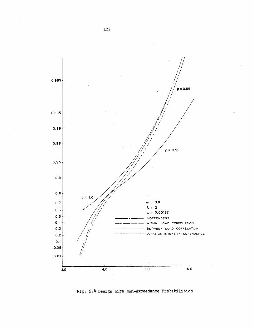
0.999
0.995
0.99
0.98
0.95·
0.9
0.8
0.7
0.6
0.5
0.4
0.3
0.2
0.1
0.05
0.01
3.0
122
-------
4.0
I
// I I
1/ I I I
I P = 0.99 I
I I
P : 0.99
W : 3.0
A : 2
J.L = 0.00137
INDEPENDENT
WITHIN LOAD CORRELATION
BETWEEN LOAD CORRELATION
DURATION-INTENSITY DEPENDENCE
5.0 6.0
Fig. 5.4 Design Life Non-exceedance Probabilities
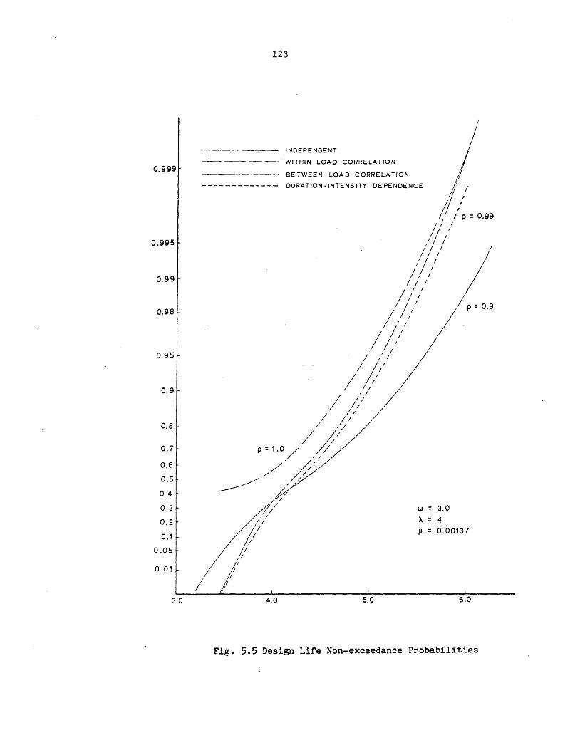
0.999
0.995
0.99
0.98
0.95
0.9
0.8
0.7
0.6
0.5
0.4
0.3
0.2
0.1
0.05
0.01
3.0
123
INDEPENDENT
WITHIN LOAD CORRELATION
BETWEEN LOAD CORRELATION
DURATION-INTENSITY DEPENDENCE
/
'7 /
/
, I
f' , I /1
4.0 5.0
w = 3.0
A = 4
p = 0.9
~ = 0.00137
6.0
Fig. 5.5 Design Life Non-exceedance Probabilities
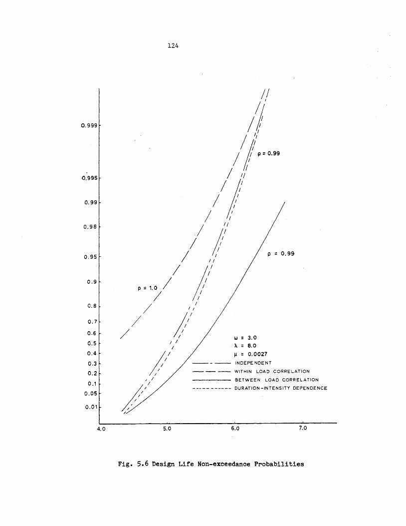
0.999
0.995
0.99
0.98
0.95
0.9
0.8
0.7
0.6
0.5
0.4
0.3
0.2
o. , 0.05
0.01 t 4.0
124
II
/J' // / I! p = 0.99
1;1 / / ,/
/ ;'
/ / / II / It' / !/
p = 1.0 / /
/ / / '/
/ // / //
w = 3.0 . h = B.O
p = 0.99
J.l = 0.0027
----- INDEPENDENT
- - -- WITHIN LOAD CORRELATION
5.0
BETWEEN LOAD CORRELATION
----- ------ DURATION-INTENSITY DEPENDENCE
6.0 7.0
Fig. 5.6 Design Life Non-exceedance Probabilities
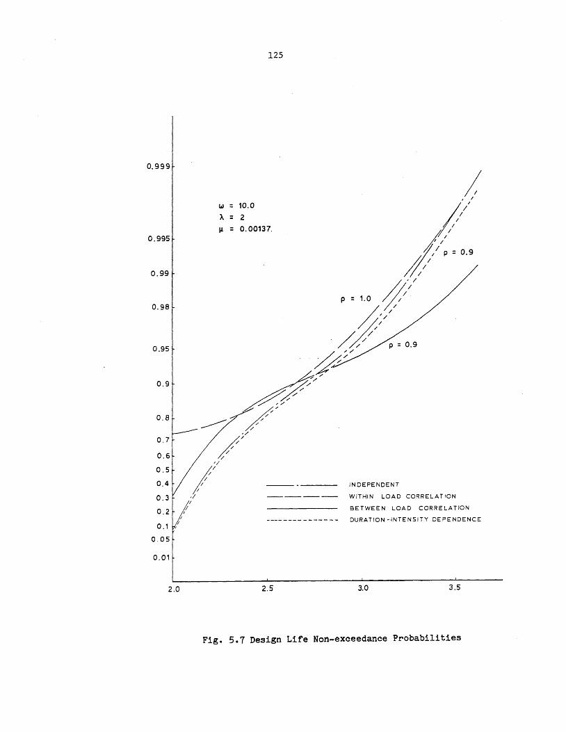
0.999
0.995
0.99
0.98
0.95
0.9
0.8
0.7
0.6
0.5
0.4
0.3
0.2
0.1 /
0.05
0.01
2.0
I
I
I
'I
w = 10.0
A = 2
125
~ = 0.00137.
--------
2.5
INDEPENDENT
WITHIN LOAD CORRELATION
BETWEEN LOAD CORRELATION
DURATION -INTENSITY DEPENDENCE
3.0 3.5
Fig. 5.7 Design Life Non-exceedance Probabilities
0.999
0.995
0.99
0.98
0.95
0.9
0.8
0.7
0.6
0.5
0.4
0.3
0.2
o. , 0.05
0.0'
2.5
126
INDEPENDENT
-- -- - -- WITHIN LOAD CORRELATION
BETWEEN LOAD CORRELATION
DURATION-IN TENSITY DEPENDENCE
/
/ /
p = 1.0/ /
/
,/ yo
/
tAl = 10.0
A = 8
~ = 0.0027
/ /
3.0
/ /
/ /
/
3.5
/ /
0.9
p = 0.9
4.0
Fig. 5.8 Design Life Non-exceedance Probabilities
S2( t)
127
Lo-t:::. X,
0
1 id'i L
------0-0-6 x_ j ~ ~ T,
t Cluster ing
\
I
I I I f
I . I
I I I I I I ·1
----; T, ~ I \ : Clustering I I I I I
I A I X2
I I
;0 I I I
X--O-t:::. O-l:::. ~--LlL[l--L-------" -J ~ ~ ~
o Parent (generating) point process
6 Delayed point process
x T.
1 X. ,
Noise process
(Random) delay time Intensity given occurrence
d; duration given occurrence
~~
Fig. 5.9 Model for Occurrence Clustering
CLUSTERING
IN DEPENDENT
w = 3.0 0.05
Ae = /YR
As = 4 /YR
~e = 20.0 5
~a = 10.0 s
128
/ /
/ I
I I
I I I
/// I I
/// I I
// I I
/// I I
// I / e
/ I
/ I
I I
I
I I
/
/ I
/ I
/ / I r ·1 /
'1/ / / ~ QUA K E '---~~ - .~~ 'H+A f-t-Ptl\ "-+i-I~ H-HA A++-+D 01AAPt"· 0 ~ .. ~"'-"'"-. • AvJv vV ITVVVV U V "YO y'
/ 5 R V l'--+I_-----l(\I....4-+!\4-+-f'\.\--,A-.... _ \[VV
I. e .1. 5 .1
5.0 6.0 7.0 r
Fig. 5.10 Combined Nonstationary Earthquake and SRV Response
129
THRESHOLD r
3 4 5
-------LRF
C = 0.75
-1 10 ~
103 LOAD COl NCIDENCE
Fig. 6.1 Exceedance Probabilities of LRF and Load Coincidence
130
APPENDIX A
TIME INVARIANT RELIABILITY MEASURES
The well known Hasofer/Lind reliability index is a measure of the
reliability of a component when only second moment information of the
basic design variables is available.
The failure surface (limit state) of the compnoent is given in the
form
(A.1)
This surface divides the design space into two regions; a safe region in
which g(X»O and a failure region in which g(X)<O. To obtain the
Hasofer/Lind reliability index ~HL' the limit surface is transformed
into a space of standardized variates
(A.2)
In this transformed space ~HL is the minimum distance from the origin
to the limit surface
. Ff m~n/u'" u
131
For those cases in which the probability distribution of the basic
variables is known or may be assumed, a more formal approach may be
taken. If the limit state is linear and the variables are Gaussian, the
reliability may be calculated exactly
s * L ct. u. ~ ~
i
(A.4)
... ai are the direction cosines; ui are the coordinates of a point on the
surface in standardized space.
In general, the limit surface will be a nonlinear function of the
load and resistance variables, and the variables will not necessarily be
Gaussian. For systems with high reliability or for relatively flat
failure surfaces, a linearization of the surface will allow computation
of the reliability with good approximation.
Let the basic variables Xi have distributions Fi and be
independent. For correlated variables the reader should see
Hohenbichler and Rackwitz (1981). Transform the variables and the limit
surface to unit normal space.
Transformation: <I> (y .) = F. (x. ) ~ ~ ~
g(F-l[<I>(Yi)]) = 0 (A.S)
Limit surface :
Consider the point yO = (y~, Y2, ... ,y~) on the surface and
linearize the surface at this pOint. The plane, tangent to the limit
surface at this pOint has the equation
where (A.6)
132
The tangent plane approximates the true failure surface and also divides
the space into a safe and a failure region as shown in Fig. A.1. Define
the distance from the origin to the orthogonal projection pOint on the
plane as {3(yO), Fig. A.2. The approximate r,eliability given by the
linearization is
Define the true reliability as R. The error produced by the
linearization is
(A.8)
This error represents the integral of the probability density over the
shaded region in Fig. A.1. The optimum linearization point is that
point which minimizes the error €. Note that this is true for any
distribution functions for which L(yO) may be readily calculated, and
not necessarily only for Gaussian variables.
From Eqs. A.7 and A.8 we deduce that the optimum point is obtained
by finding the minimum of the local stationary points of {3(yo), where
S(yO) L ° Cl. Yi i
l.
c. (A.9) l.
a.. c~]1/2 l. [L
j J

133
In the rotationally symmetric unit normal space it can be shown
(CIRIA, 1977) that the optimum linearization point will coincide with
the point on the surface closest to the origin (Hasofer/Lind point). It
is easy to see that this pOint is also the point of maximum probability
denSity on the surface.
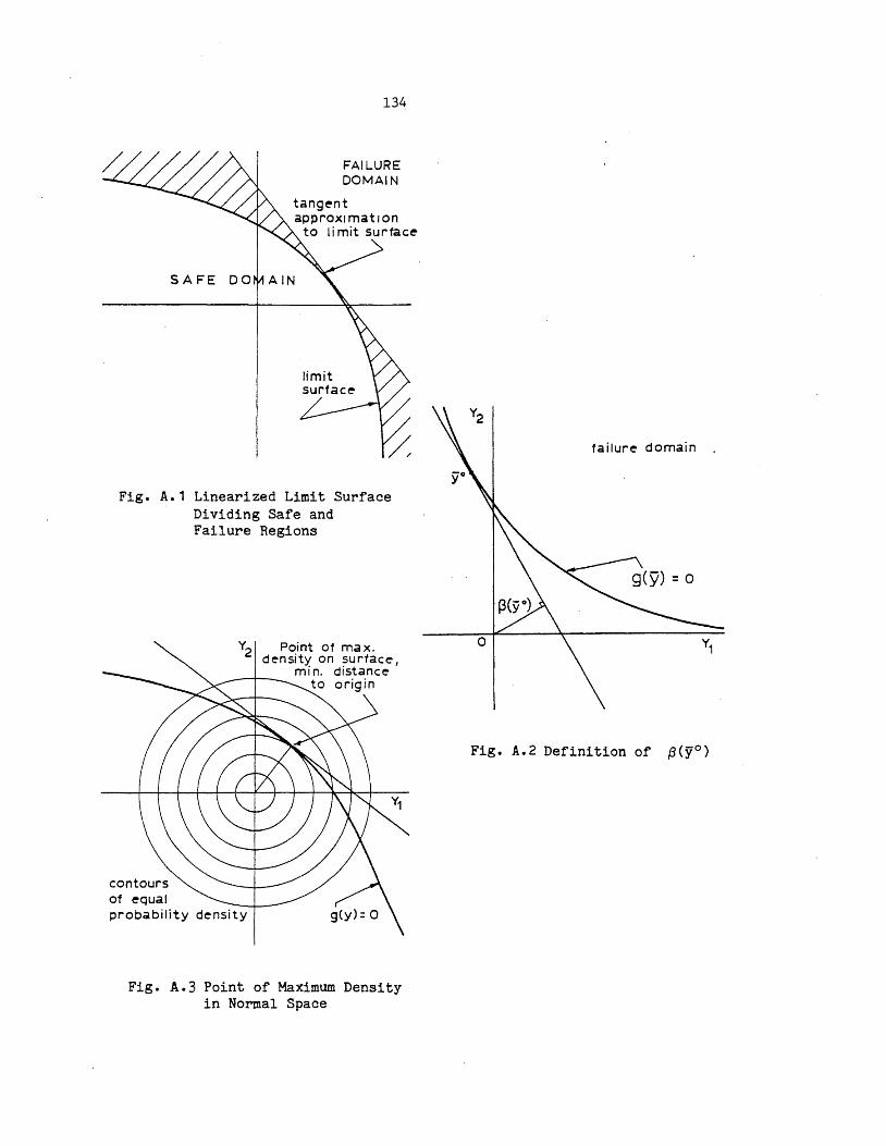
134
FAILURE DOMAIN
tangent approXImation
to I i mit surface
Fig. A.1 Linearized Limit Surface Dividing Safe and Failure Regions
Y2 Point of ma x. density on surface I
contours of equal probability density
min. distance to origin
Fig. A.3 Point of Maximum Density in Normal Space
failure domain
9(9) = 0
o
Fig. A.2 Definition of ~(yO)
135
APPENDIX B
THE RACKWITZ/FIESSLER ALGORITHM
For an n-dimensional reliability problem it is necessary to
evaluate an n-dimensional integral of the joint density function of the
basic variables over the safe domain. The transformation to normal
space and the approximation of the n-dimensional integral over the safe
domain by a single integral for a linearized domain has been termed fast
convolution (Lind, 1980; Dit1evsen, 1980). The procedure used in fast
convolution is the Rackwitz/Fiessler algorithm.
The basic variables, generally non-normal, and the limit state
function are as described in Appendix A.
The algorithm takes advantage of the fact that, in normal space,
the optimum linearization point coincides with the point on the surface
closest to the origin.
Instead of transforming the total space of basic variables into
normal space (not an easy task), the linearized safe set of the
transformed formulation space may be determined by calculations in the
original space by using the prinCiple of normal tail approximation
(Ditlevsen, 1982; Hohenbichler and Rackwitz, 1981).
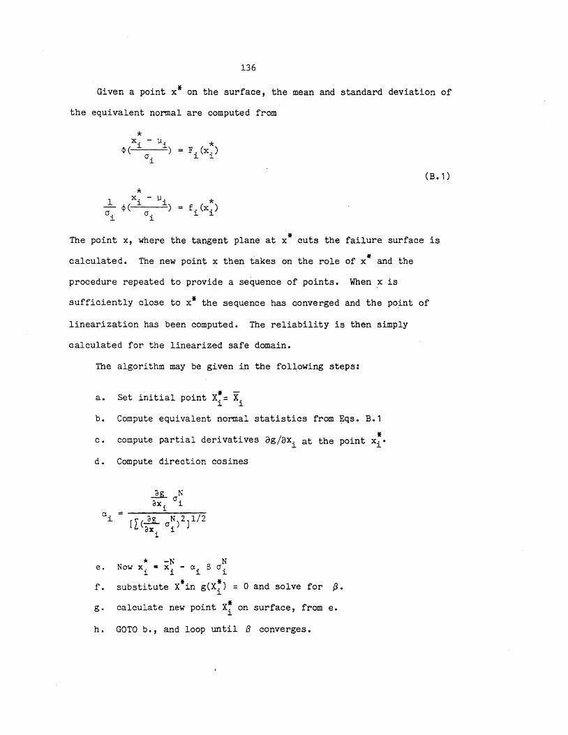
136
Given a point x* on the surface, the mean and standard deviation of
the equivalent normal are computed from
* x. - ll. <l>( ~ ~)
0. 1.
* F . ex.) ~ 1.
* f. (x.) ~ 1.
(B. 1 )
* The point x, where the tangent plane at x cuts the failure surface is
calculated. The new point x then takes on the role of x· and the
procedure repeated to provide a sequence of points. When x is
* sufficiently close to x the sequence has converged and the po~nt of
linearization has been computed. The reliability is then simply
calculated for the linearized safe domain.
The algorithm may be given in the following steps:
a.
b.
c.
d.
a.. 1.
e.
f.
g.
h.
Set initial point X~= X. ~ ~
Compute equivalent normal statistics from ~qs. B.1
* compute partial derivatives ag/axi at the point xi·
Compute direction cosines
* -N N Now xi - xi - 0.1 8 0i
substitute X·in g(X~) = 0 and solve for ~. ~
calculate new point X~ on surface, from e. ~
GOTO b., and loop un til 8 converges.
137
LIST OF REFERENCES
Ang A.H-S and Ma H.F.,"On the Reliability of structural Systems", Proc. 3rd Int. Conf. on Structural Safety and Reliability, Trondheim, Norway, June 23-25, 1981.
Belyaev Y.K., "On the Number of Exits across the Boundary of a Region by a Vector Stochastic Process" Theory of Probability with Applications, Vol. 13, 1968, pp 320-324.
Bergman L.A. "Moments of Time to First Passage of the Linear Oscillator", Ph.D Thesis, Dept. of Civil Engineering, 'Case Western Reserve University, Cleveland, OhiO, 1979.
Bergman L.A. and Heinrich J.C., "On the Reliability of the Linear Oscillator and Systems of Coupled Oscillators" Int. Jour. for Numerical Methods in Engineering, Vol. 18 (1982), pp 1271-1295
Bosshard W., "On Stochastic Load Combination" John Blume Earthquake Engineering Center, Stanford University, Report No. 16, July 1975.
Breitung K. and Rackwitz R., "Structural Reliability under Combined Random Load Sequences" Computers and Structures, Vol. 9, 1978, pp 489-494.
Breitung K. and Rackwitz R., "Upcrossing Rates for Rectangular Pulse Load Processes" Laboratory for Structural Engineering, Technical University of Munich, SFB 96, Report No. 42, 1979.
Breitung K. and Rackwitz R., "Nonlinear Combination of Load Processes" Journal of Structural Mechanics 10(2), 1982 pp 145- 1 66.
Bunge M., "Four Concepts of Probability" Applied Mathematical Modeling Vol. 5, Oct 1981, pp 306-312.
Coleman J.J., "Reliability of Aircraft Structures in Resisting Chance Failure" Operations Research 7(1959) pp 639-645.
Cornell C.A., "A Probability Based Structural Code" Jour. American Concrete Institute, Vol. 66, No. 12

138
Cornell C.A., "structural Safety: Some Historical Evidence that it is a Healthy Adolescent" Proc. ICOSSAR 1981 Trondheim, Norway. Published by Elsevier "Developments in Civil Engineering 4"
Cox D.R. and Lewis P.A.W., "Multivariate Point Processes" Proc. 6th Berkeley Symposium on Mathematical Statistics, 1912 vol. 3 pp 401-448.
Cramer H. and Leadbetter M.R., Stationary and Related Stochastic Processes Wiley, 1961.
Der Kiureghian A., "Second Moment Combination of Stochastic Loads" Journal of the Structural Div., ASCE, Vol. 104 No. ST10 Oct. 1918, pp 1551-1561.
Der Kiureghian A., "Reliability Analysis under Stochastic Loads" Jour. Structural Div., ASCE, Vol. 106, No. ST2, Feb. 1980, pp 411-429.
Ditlevsen o. and Madsen H.O., Discussion of "Optimal Reliability Analysis by Fast Convolution" Jour. Engineering' Mechanics Div., ASCE, Vol. 106, No. EM3, 1980, pp 519-583.
Ditlevsen 0., "Principal of Normal Tail Approximation" Jour. Engineering Mechainics Div., ASCE, Vol. 101, No. EM6, Dec. 1981, pp 1191-1207.
Ditlevsen O. and Madsen H.O., "Transient Load Modeling 1: Clipped Normal Processes" DCAMM, Report No. 205, March 1981, Technical University of Denmark, Lyngby, Denmark.
Ditlevsen o. and Madsen H.O., "Probabilistic Modeling of Man-made Load Processes and their Individual and Combined Effects" Proc. ICOSSAR 1981, Trondheim, Norway, June 23-25, 1981.
Ditlevsen 0., "Model Uncertainty in Structural Reliability" structural Safety, Vol. 1(1), 1982.
Ditlevsen 0., "Extended Second Moment Algebra as an Efficient Tool in Structural Reliability" Nuclear Engineering and Design 11(1982) pp 317-323.
Ellingwood B., Galambos T.V., MacGregor J.G. and Cornell C.A., "Development of a Probability Based Load Criterion for American National Standard A58" National Bureau of Standards, NBS Special Publication 577, Washington D.C. (June 1980).
Ellingwood B., "Safety Checking Formats for Limit States Design" Jour. Structural Div., ASCE, Vol. 108, No. ST7, July 1982, pp 1481-1493.
139
Ferry-Borges J. and Castanheta M., "Structural Safety" National Laboratory of Civil Engineering, Lisbon, Portugal, March 1971.
Fiessler B., Neumann H-J. and Rackwitz R., "Quadratic Limit States in structural Reliability" Jour. Engineering Mechanics Div., ASCE, Vol. 107, No. EM6, 1981, pp 1227-1238.
Galambos T.V., "Load and Resistance Factor Design" Engineering Journal, AISC, 3rd Quarter, 1981.
Galambos T.V., Ellingwood B., MacGregor J.G. and Cornell C.A., "Probability Based Load Criteria: Assessment of Current Design Practice" Jour. Structural Div., ASCE, Vol. 108, No. ST5, May 1982, pp 959-977.
Gaver D.P. and Jacobs P.A., "On Combinations of Random Loads" SIAM Jour. of Applied Mathematics, Vol. 40, No.3, June 1981, pp 454-466.
George L.L., "A Comparison of some Probability Distributions of Peak Combined Responses" 7th SMiRT, Paris, France, 1981.
Grigoriu M., "Methods for Approximate Reliability Analysis" Strutural Safety, 1(1982/1983) pp 155-165, Elsevier.
Hasofer A.M. and Lind N.C., "An Exact and Invariant First Order Reli:::bility Format" Jour. Engineering Mechanics Div., ASCE, Vol. 1 ° ° , No • EM 1, 1 974 , p p 111 - 1 2 1 •
Hasofer A.M., "Time Dependent Maximum of Floor Live Loads" Jour. Engineering Mechanics Div., ASCE, Vol. 100, No. EM5, Oct. 1974, pp 1086-1091.
Hohenbichler M. and Rackwitz R., "Non-normal Dependent Vectors in Structural Safety" Jour. Engineering Mechanics Div., ASCE, Vol. 107, No. EM6, Dec. 1981, pp 1227-1238.
Ingles O.G., "Safety in Civil Engineering - its perception and promotion" Reliability Engineering 1(1980) pp 15-27.
Larrabee R.D., "Approximate Stochastic Analysis of Combined Loading" Research Report CER 78-28, M.I.T., Sept. 1978.
Larrabee R.D. and Cornell C.A., "Upcrossing Rate Solution for Load Combinations" Jour. Structural Div., ASCE, Vol. 105, No. 3T1, Jan. 1979, pp 125-132.
Larrabee R.D. and Cornell C.A., "Combination of Various Load Processes" Jour. Structural Div., ASCE, Vol. 107, No. ST1, Jan. 1981, pp 223-239.
Lin Y.K., Probabilistic Theory of Structural Dynamics Krieger Publishing Co., Huntington, New York, 1976.

140
Lind N.C., "Optimal Reliability Analysis by Fast Convolution" Journal of the Engineering Mechanics Division, ASCE, Vol 105, No EM3, June 1979, pp 447-452.
Lutes L.D., Chen Y-T. and Tzuang S-H., "First Passage Approximations for Simple Oscillators" Jour. Engineering Mechanics Div., ASCE, Vol. 107, No. EM6, Dec. 1980, pp 1111-1124.
Madsen H., Kilcup R. and Cornell CoA., "Mean Upcrossing Rate for Sums of Pulse-type Stochastic Load Processes" Proc. Specialty Conf. on Probabilistic Mechanics and Structural Reliability, Tucson, Arizona, Jan. 1979.
Madsen H.O., "Load Models and Load Combinations" Report No R113, Feb1979, Structural Research Laboratory, Technical University of Denmark, Lyngby.
Madsen H.D. and Ditlevsen 0., "T~ansient Load Modeling II: Markov Rectangular Pulse Processes" DCAMM Report, 1981, Technical University of Denmark, Lyngby, Denmark.
Mattu R.K., "Methodology for Combining Dynamic Responses" Nureg-0484, U.S. NRC (May 1980).
Pearce H.T. and Wen Y-K., "On Linearization Points for Nonlinear Combination of Stochastic Load Processes" submitted to Structural Safety, Elsevier Publishirig Co.
Peir J.C. and Cornell C.A., "Spatial and Temporal Variability of Live Loads" Jour. Structural Div., ASCE, Vol. 99, No. ST5, May 1913, pp 903-922.
Rackwitz R. and Fiessler B., "Structural Reliability under Combined Random Load Sequences" Computers and Structures Vol. 9, 1918, pp 489-494.
Ravindra H.K. and Lind N.C., "Theory of Structural Code Optimization" Jour. Structural Div., ASCE, Vol. 99, ST7, July 1913, pp 1541-1553.
Ravindra H.K., "Probability Based Design Criteria for Nuclear Structures" Nuclear Engineering and Design, 59(1980), pp 197-204.
Rice S.O., "Mathematical Analysis of Random Noise" in Selected Papers on Noise and Stochastic Processes N. Wax (Ed.), Dover Publications.
Schwartz M.W., Ravindra M.K., Cornell C.A. and Chou C.K., "Load Combination Methodology Development" Project II Final Report, NuregCR-2081, ucrl-53025, Sept. 1981.
141
Shinozuka M., "Probability of Structural Failure under Random Loading" Jour. Engineering Mechanics Div., ASCE, Vol. 90, No. EMS, Dec. 1964, pp 147-171.
Shinozuka M. and Tan R., "Probabilistic Load Combination and Crossing Rates" Proc. Symp. on Probabilistic Methods in Structural Engineering, ASCE, St. Louis, Missouri, Oct. 26-27, 1981.
Shinozuka M. "Basic Analysis of Structural Safety" Jour. of Structural Engineering, ASCE, Vol. 109, No.3, March 1983, pp 721-740.
Siu W.W.C., Parimi S.R. and Lind N.C., "Practical Approach to Code Calibration" Jour. Structural Di v., ASCE, Vol. 101, No. ST7, July 1975, pp 1469-1480.
Stevenson J.D., "Current Summary of International Extreme Load Design Requirements for Nuclear Power Plant Facilities" Nuclear Engineering and DeSign, 60(1980), pp 197-209.
Turkstra C.J., "Theory of Structural DeSign Decision"· UniverSity of Waterloo, Waterloo, Ontario, Canada 1970.
Turkstra C. and Madsen H.O., "Load Combination in Codified Structural Design" Jour. Structural Div., ASCE, Vol. 106, No. 3T12, Dec. 1980.
Vanmarcke E.H., "On the Distribution of the First Passage Time for Normal Stationary Random Processes" Trans. of ASME Vol. 42, Series E, Journal of Applied Mechanics, No.1, March 1975.
Veneziano D., Grigoriu M. and Cornell C.A., "Vector-process Models for System Reliability" Jour. Engineering Mechanics Div., ASCE, Vol. 103, No. EM3, June 1977, pp 441-460.
Wen Y-K., "statistical Combination of Extreme Loads" Jour. Structural Div., ASCE, Vol. 103, No. ST5, May 1977, pp 1079-1093.
Wen Y-K., "Equivalent Linearization for Hysteretic System under Random Excitation" Journal of Applied Mechanics, Trans. ASME, Vol. 47, No.1, March 1980.
Wen Y-K., "Methods for Reliability of structures under Multiple Time Varying Loads" Nuclear Engineering and Design, 60(1980), pp 61-71.
Wen Y-K., "Reliability Analysis under the Combination of Stochastic Loads" Proc. Int. Specialty Conf. on the Probabilistic Safety of Structures, Sept. 1980, Paris, France.
Wen Y-K. and Pearce H.T., " Stochastic Models for Dependent

142
Load Processes" Structural Research Series No. 489, UILU-ENG-81-2002, Civil Engineering Studies, University of Illinois, Urbana, Illinois, March 1981.
Wen Y-K. and Pearce H.T., "Recent Developments in Probabilistic Load Combination" Proc. Symp. on Probabilistic Methods in Structurual Engineering, ASCE, St. Louis, Missouri, Oct. 26-27, 1981.
Wen Y-k., "A Clustering Model for Correlated Load Processes" Jour. Structural Div., ASCE, Vol. 107, No. ST5, May 1981, pp 965-983.
Wen Y-k. and Pearce H.T., "Combined Dynamic Effects of Correlated Load Processes" to appear in Nuclear Engineering and DeSign, 1983.
Winterstein S.R., "Combined Dynamic Response: Extremes and Fatigue Damage" Dept. of Civil Engineering, M.I.T., Report R80-46, Dec. 1980.
Yang J.N. and Shinozuka M., "On the First Excursion Probability in Stationary Narrow-Band Random Vibration" ASME, Journal of Applied Mechanics, Vol. 38, Dec. 1971, pp 1017-1022.
Yang J.N. and Shinozuka M., "On the First Excursion Probability in Stationary Narrow-Band Random Vibration II" ASME, Journal of Applied Mechanics, Vol. 39, Sept. 1972, pp 733-738.


![A Stochastic Optimization Method for Energy-Based …deepakns/PDF/Subramani_etal_DyDESS2015.pdfA Stochastic Optimization Method ... safety or a combination of these [12,16]. ... by](https://img.pdfslide.us/doc/110x75/5af372b57f8b9a8b4c9185aa/a-stochastic-optimization-method-for-energy-based-deepaknspdfsubramanietal.jpg)