Embed Size (px)
Citation preview

IISF/RA 800015UILU-ENG 80-2004
Technical Report of ResearchSupported by the
National Science Foundationunder
Grant ENV 77-09090
by
J. Mohammadi
and
A. H-S. Ang
EAS 1NFORMATION RESOURCES; NATIONAL SCIENCE FOUNOATION
DEPARTMENT OF CIVIL ENGINEERING
UNIVERSITY OF IlliNOIS
AT URBANA-CHAMPAIGN
FEBRUARY 1980
~ ,> J
A METHOD FOR THE ANALYSIS OFSEISMIC RELIABILITY OF LIFELINE SYSTEMS
CIVIL ENGINEERING STUDIESStrudural Research Series No. 474

ii
ACKNOWLEDGMENTS
This report is based on the doctoral dissertation of J. Mohammadi
submitted to the Graduate College of the University of Illinois at
Urbana-Champaign in partial fulfillment of the requirements for the
Ph.D. degree. The study was directed by Dr. A. H-S. Ang, Professor of
Civil Engineering as part of a research program on the evaluation of
safety of structures to earthquakes and other natural hazards, and is
supported by the National Science Foundation under Grant ENV 77-09090.
This support is gratefully acknowledged.
Any opinions, findings, conclusionsor recommendations expressed in thispublication are those of the author(s)and do not necessarily reflect the viewsof the National Science Foundation.

------~------~-----~------------~---

CHAPTER
1
2
3
4
iii
TABLE OF CONTENTS
INTRODUCTION .
1.1 Introductory Remarks . . ...1. 2 Review of Re1 ated Work. ..1.3 Objective and Scope of Study ...•.1.4 Notation .
ATTENUATION EQUATION FOR NEAR-SOURCE REGIONS.
2.1 Introductory Remarks .2.2 Effect of Earthquake Magnitude .2.3 Wave Propagation in Half-Space Solids..2.4 Acceleration, Velocity, and Displacement
in Vertical and Horizontal Motions ..2.5 Variation of Intensity in Near-Source
Regions. . . . . . . . . .2.5.1 The Strike-Slip Case..•.....•2.5.2 The Dip-Slip Case .
2.6 Comparison with Existing AttenuationEquations. . . . . . . . . . . . . .
RELATIONSHIPS NEEDED IN SEISMIC RISK ANALYSIS
3.1 Earthquake Mechanism .3.2 Earthquake Magnitude and Slip Length.3.3 Modeling Potential Earthquake Sources...
MODELS FOR SEISMIC HAZARD ANALYSIS OFLIFELINE SYSTEr4S....
4.1 Introductory Remarks .4.2 Fault-Rupture Hazard . . . . . .. • •..4.3 Determination of P(LjIEi) ....
4.3.1 Type 1 Source (Well-definedfaults system) .
4.3.2 Type 2 Source (Dominant faultdirection known) .
4.3.3 Type 3 Source (Unknown faults).4.4 Hazard from Severe Ground Shaking.4.5 Critical Section of a Link .
Page
1
1246
8
89
12
15
16
1719
23
26
262730
32
323336
37
39404345
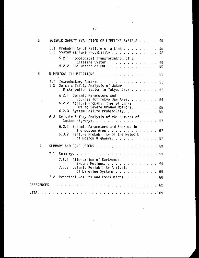
6.1 Introductory Remarks . . . . . . . 536.2 Seismic Safety Analysis of Water
Distribution System in Tokyo, Japan. . 536.2.1 Seismic Parameters and
Sources for Tokyo Bay Area. . 546.2.2 Failure Probabilities of Links
Due to Severe Ground Motions. . 556.2.3 System Fa i 1ure Probabi 1i ty. . . . . 55
6.3 Seismic Safety Analysis of the Network ofBoston Highways. . . . . . . . . . . . 57
6.3.1 Seismic Parameters and Sources inthe Boston Area . . . . . . .. .... 57
6.3.2 Failure Probability of the Networkof Boston Highways. . 57
REFERENCES. .
VITA....
4950
53
• 46
59
59
59
59
60
62
. . 109
. . . 46. 48
Summary .7.1.1 Attenuation of Earthquake
Ground Motions. . . . .7.1.2 Seismic Reliability Analysis
of Lifeline Systems ...Principal Results and Conclusions.•
iv
7.1
NUMERICAL ILLUSTRATIONS . . . . .
SEISMIC SAFETY EVALUATION OF LIFELINE SYSTEMS
5.1 Probability of Failure of a Link .5.2 System Failure Probability .
5.2.1 Topological Transformation of aLifeline System ...
5.2.2 The Method of PNET.· .
7.2
SUM~~RY AND CONCLUSIONS7
5
6

TABLE
2. 1
2.2
2.3
2.4
2.5
4. 1
6.1
6.2
6.3
6.4
6.5
v
LIST OF TABLES
SUM~~RY OF VERTICAL TO HORIZONTALACCELERATION RATIOS . . . . . .
SUM~~RY OF VERTICAL TO HORIZONTAL viaRATIOS .
SUMt~RY OF AVERAGE ad/v2 VALUES
SUMMARY OF AVERAGE vIa . . . . .
GROUND MOTION ATTENUATION EQUATIONS. .
VALUES OF e FOR TYPE 3 SOURCE.....
ANNUAL PROBABILITY OF FAILURE IN A PATH(TOKYO) .
ANNUAL PROBABILITY OF FAILURE OF SUPPLYNETWORK (TOKYO) .
IDEALIZATION OF SOURCES FOR BOSTON AREA..
ANNUAL FAILURE PROBABILITY OF LINK . . .
EQUIVALENT PARALLEL PATHS FOR BOSTON HIGHWAYS
Page
67
67
68
69
70
71
72
73
74
75
76

---------------~-------------------------
vi
LIST OF FIGURES
VARIATION OF a 10 WITH 0 FOR DIFFERENT Wz z - . .(h = 15 km, y = 900 ) • . . • • • • • • • • • • • • • • 79
VARIATION OF az/Dz WITH 0 FOR DIFFERENT W(h = 20 km, y ::: 900 ) . . . . . . . . ... • . . . 80
VARIATION OF a IDz WITH WFOR h = 15AN 0 y ::: 900 z. . . . . . . . . . .. .. . . . . . 81
VARIATION OF az/Dz WITH 0 FOR DIFFERENT h(y = 900
, W= 4 km). • . . • • . • • • • • • • • • • • 82
VARIATION OF a 10 WITH 0 FOR DIFFERENT h° z z
(y ::: 90 • W::: 10 km) •.•..•••....•.•.. 83
VARIATION OF az/Dz WITH D FOR DIFFERENT y
(h ::: 15, W ::: 4 km ) . • • . • • • . . • • . . . • • . • 84
VARIATION OF az/Dz WITH 0 FOR DIFFERENT y
(h ::: 15, W= 20 km). . . . • . . . . . . . . . . • . . 85
VARIATION OF a 10 WITH D FOR DIFFERENTWy x(h ::: 15, y = 900 , vp/vS ::: 1.75) 86
VARIATION OF a ID WITH 0 FOR DIFFERENT Wy x °
(h ::: 20 km, y = 90 , vp/vS ::: 1.75) . . . . . . . . . . 87
VARIATION OF a lOx WITH D FOR DIFFERENT hy °(w ::: 4 km, y ::: 90 , vp/vS ::: 1.75). . . . . . . . . . . 88
VARIATION OF a 10 WITH D FOR DIFFERENTy x °vp/vS (h = 15, W= 4 km, y ::: 90) . . . . . . . . . . 89
77
78
78
Page
. . . . . . . .t4AGNITUDE VERSUS 01 N FOR M2. 4 ...
TWO-DIMENSIONAL FAULT r·10DEL (DIP-SLIP)
TWO-DIMENSIONAL FAULT MODEL (STRIKE-SLIP).
FIGURE
2.1
2.2
2.3
2.4
2.8a
2.5
2.12
2.7a
2.9
2.6
2.7b
2. 11
2.8b
2.10

--- - ~ --- ~ ----------------------
vii
105
104
102
103
98
98
98
99
99
100
101
. . . . . . .
Page
VARIATION OF a 10 WITH 0 FOR DIFFERENT,yy x(h = 15, W = 4 km, vp/vS = 1.75). . .. 90
VARIATION OF a 10 WITH D FOR DIFFERENT Wx x(h = 15 km, y = 90°, vp/vS =.1. 75). • • • • • . . .. 91
VARIATION OF a 10 WITH 0 FOR DIFFERENT Wx x °
(h = 20 km, y = 90 , vp/vS
= 1.75). • • • . • • • .• 92
VARIATION OF a/ox WITH D FOR DIFFERENT h(W = 4 km, y = 90°, vp/vS = 1.75) . . . . . . . . .. 93
VARIATION OF a ID WITH 0 FOR DIFFERENTx xvp/vS (W = 4, h = 15 km, y = 90°) .. 94
VARIATION OF a /0 WITH 0 FOR DIFFERENT yx x
(W = 4, h = 15 km, vp/vS = 1.75). . . . . . . . . .. 95
ATTENUATION OF MAXIMUM GROUND ACCELERATION(m = 7.0) . . . . . . . . 96
SIMPLE LIFELINE NETWORKS. . 97
TYPE 1 SOURCE .
TYPE 2 SOURCE
TYPE 3 SOURCE
ANNUAL PROBABILITY OF EXCEEDANCE.
PDF OF LINK RESISTANCE. . .
A NETWORK OF PARALLEL PATHS . .
WATER SUPPLY NETWORK FOR TOKYO.
EPICENTER MAP OF TOKYO BAY AREA(1961-1970). . . . . . . . .
MAGNITUDE RECURRENCE CURVE. . . .
EQUIVALENT PARALLEL NETWORKS FOR TOKYO. .
FAILURE PROBABILITY, NETWORKS A + 9 ANDB + 9 (HAZARD OF GROUND SHAKING)....
2. 19
2.16
2.15
2.14
2.17
2.18
FIGURE
2.13
4. 1
4.2
4.3
4.4
5.1
5.2
5.3
6.1
6.2
6.3
6.4
6.5

FIGURE
6.6
6.7
6.8
viii
FAILURE PROBABILITY, NEnJORK C+ 9(HAZARD OF GROUND SHAKING). . ...
BOSTON ~~JOR HIGHWAYS . . . . . . .
IMPORTANT EARTHQUAKES IN BOSTON AREA . . . •.
Page
106
107
108


1
CHAPTER 1
INTRODUCTION
1.1 Introductory Remarks
The reliability of a lifeline system against earthquake hazards, in
an area of high seismic activity, is one of the most important factors
that need to be considered in its design. The term "lifeline system,"
as used here, refers to networks of man-made or engineered systems covering
vast surface areas. By this definition, oil pipelines, water distribution
systems, communication, or transportation networks are all considered as
lifeline systems.
In a seismically active region, the time of occurrence, location,
and size as well as other characteristics of future earthquakes are not
predictable. Therefore, the analysis of earthquake effects on a lifeline
system requires probability consideration. More specifically, the design
of a lifeline system, in an area of earthquake activity, properly requires
the probabilistic assessment of the destructive potentials of future
earthquakes and the risk associated with the damage that could conceivably
befall the system. The damages may be either because of the fault rupture
striking on one or more links of a lifeline system or the failure of the
links caused by high intensity ground motions exceeding the resistance
capacity of the links.
In the case of a building or nuclear power plant, the spatial
dimension of the structure is negligible, and may be assumed to be a
point structure. The seismic risk analysis of a point structure, therefore

2
may be limited to the probabilistic assessment of future ground motion
intensities at the point. In other words, the probability that the
maximum ground motion of a given site will exceed a specified intensity
within a given time interval is considered; the results may be expressed
in terms of the annual exceedance probability, or its inverse, the
average return period in years. In this case the chance of a fault
rupture striking the point is extremely remote.
In contrast to a point system, the significant areal coverage or
vast spatial expanse of a·lifeline system requires a different approach
from that of a point system. In this case, the risk associated with a
fault-rupture intersecting one or more links of the system can be signifi
cant and must be considered in addition to the failure of the links
caused by high seismic intensity exceeding the resistance of the links.
In other words, in the case of a lifeline system, two modes of seismic
hazards may be involved.
1.2 Review of Related Work
Seismic risk analysis has been mainly restricted to point systems,
and it has been only in recent years that the subject is extended to
lifeline systems (e.g. Campbell, et al ,1978; Duke and Moran, 1975;
Shinozuka, et al , 1978; and Taleb-Agha, 1977). In one of the first
studies on the reliability of lifeline systems, a system was modeled as
a network of interconnected links and the probability that the network
will function properly after the occurrence of an earthquake of random
magnitude and location was evaluated. Later, Taleb-Agha (1977) assumed the
resistance of each link as an independent random variable and extended
the above model so that it can be used in networks of larger size. Recently,

3
Shinozuka, et 01. (1978) considered the free-field strains as the resistance
and developed a method for seismic risk analysis of underground pipeline
systems. This model was used for the water distribution system of the
city of Tokyo, Japan.
Among the recent studies, Duke and Moran (1975), and Campbell,
et al (1978) discussed the problem of the seismic risk analysis of a
lifeline system and gave guidelines for evaluating the reliability of
lifelines against earthquakes. The importance of organizing design
procedures for lifelines similar to those for buildings was stressed.
In the analysis of seismic risk, a major source of uncertainty is in
the attenuation equation (Der-Kiureghian and Ang, 1977). This is
particularly true for the near-source regions. The problem of the near
source regions is particularly important in the case of the seismic risk
analysis of lifeline systems; because of the vast areal coverage of a
lifeline system, some links may be very close to the fault-rupture of an
earthquake. In such cases, because of uncertainty in the available
attenuation equations for close-in regions, a suitable relation may be
derived based on analytical models of wave propagation. Among the recent
developments of wave propagation in half-space solids (e.g. Refs. 6,
44) is the study of Seyyedian and Robinson (1975). In this model, the
three-dimensional problem of wave propagation initiated by a fault
rupture in a half-space is idealized as two two-dimensional problems, as
follows: (i) a plane-strain problem; and (ii) an antiplane problem.
The complete state of displacement for the close-in regions may then be
obtained by properly combining the solutions to the above two problems.

-~-----~_.~-~~-----
4
The information thus obtained may be useful for establishing an intensity
distance-magnitude relationship especially applicable for the near-source
regions.
1.3 Objective and Scope of Study
Tectonic earthquakes originate as ruptures along geologic faults,
Housner (1975) and Newmark and Rosenblueth (1971). The length of the
rupture depends on the size of a quake and may be several hundred kilometers
long for a large earthquake; the destructive force during an earthquake is
released along the entire length of the break.
In the case of a lifeline system located in a region of seismic
activity, there is always the possibility that the rupture may strike one
or more links of the system. This mode of failure could be important in
the design of lifeline systems, especially in regions where earthquakes
are of shallow foci. Of course, the links may also fail as a result of
the effect of the destructive force released during an earthquake exceeding
the resistance of the links.
The primary objective of this study is to apply the fault-rupture model
of Der-Kiureghian and Ang (1977) to the seismic risk analysis of a lifeline
system, and also to develop a companion model for evaluating the hazard
offaLilt-rupture strike on a lifeline system. Because of the importance of
the near-source regions in the seismic risk analysis of a lifeline system,
an attenuation equation for the near-source region is also developed based
on an analytical study.
In Chapter 2, the basic theory and assumptions related to the wave
propagation model used in this study is described; and the variation of

5
intensity versus distance for different geometrical and geological para
meters, associated with an earthquake source, is studied. The development
of a model for the attenuation of intensity and the comparisons with
existing attenuation equations are also presented in this chapter.
The basic assumptions regarding the proposed method of seismic risk
analysis of lifeline systems are discussed in Chapter 3 along with the
description of the three types of potential sources used in this study.
In Chapter 4, the description of a lifeline system is presented; and
the possible modes of failure of a system are introduced and discussed.
Also in this chapter the methods of evaluating the risk associated with the
fault-rupture strike of a link and the probability of failure of a link
due to ground shaking during an earthquake are presented. The probabilities
associated with the failure of individual links are the basic information
used to determine the failure probability of a lifeline system in either
mode of failure; these are presented in Chapter 5.
Numerical examples and illustrations are presented in Chapter 6.
The first example pertains to the probabilities of failure of the water
distribution system of the city of Tokyo, Japan. The results are presented
for the ground shaking hazards in terms of the annual probabilities of
failure for different mean resistances.
In the second example problem, the safety of the network of highways
around Boston, Massachusetts against fault-rupture hazard and ground
shaking is analyzed.
Chapter 7 presents the summary and major conclusions of the present
study.
6
1.4 Notation
= maximum ground acceleration;
= a seismically active area;
= surface distance from a site to an earthquake source,
also distance between ~Ai and 1ink j;
= di stan ce terms in type 1 source;
= fault di spl acement in dip-slip;
= fault displacement in strike-slip;
= maximum ground displacement;
= occurrence of an earthquake in source i;
or slip length s;
= occurrence of an earthquake in source i with magnitude m,
= a function of m and r.
= a function of x;
= probabi 1ity density function of X;
= probabi 1ity distribution function of X;
= depth of an earthquake source;
= rupture length;
= the 1ength of link j;
= occurrence of a fault-rupture strike on link j;
= upper-bound magnitude;
= a random variable describing earthquake magnitude;
= earthquake magnitude;
= lower-bound magnitude;
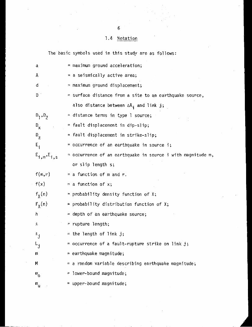
The basic symbols used in this study are as follows:
a
A
d
°°1,°2
Ox
°zE.
1
E. ,E.l,m 1, S
f(m,r)
f(x)
fX(n)
FX(n)
h
M
Q, •J
L.J
m

N(m)
PF
PF.J
r
s
S
ux,uy,uzIT
ux,uy,uzv
W
y
Y
Yr
Yr
S
Q
Y
It
~
v, vA' v.1
0, 0.1
p. .1 ,J
1/J
ep
7
= number of earthquakes with magnitude m or greater;
= system failure probability;
= failure probability of link j;
= distance of a point from a ruptured area;
= rupture length;
= a random variable describing the length of the rupture;
= components of displacement at a point;
= a vector describing the displacement at a point;
= complex functions defining u , u and u .x y z'
maximum ground velocity;
= fault width;
= intensity of the ground shaking;
= a random variable describing y;
= an intensity level for a link;
= mean intensity resistance of a link;
= regional seismicity parameter;
= C.O.v. of a link resistance;
= angle of fault orientation, also stress drop;-"
= Lame constant;
= modulus of rupture;
= earthquake occurrence rates;
= standard deviations;
= correlation coefficient between two paths i and j;
= a vector potential function; and,
= a scalar potential function, also standard normal distri-
but i on function.

~ - ---~---- ~--~- -~ - ~~~~
8
(2.1)b m -b
y = b1e 2 [f(r)] 3
2.1 Introductory Remarks
CHAPTER 2
ATTENUATION EQUATION FOR NEAR-SOURCE REGIONS
developed by several authors (e.g. Donovan, 1973, 1974; Esteva, 1970;
Kanai, 1961, 1966; McGuire, 1974; and Trifunac and Brady, 1975). These are
In the seismic risk analysis of structures and lifeline systems, a
relationship between intensity and distance and magnitude is required to
define the intensity at a point; i.e. a structure or any point of a lifeline
system. Equations in this form, known as "attenuation equations," have been
generally in the form of,
where y is the ground motion intensity at an observation point, m is the
earthquake magnitude in the Richter scale, r is the distance (epicentral,
focal, or the distance from the causative fault), bl , b2, and b3 are
constant parameters, and f(r) is a function of the distance r.
The eXisting empirical attenuation equations are mainly based on
historical earthquake data; such data are almost entirely for points
relatively far from the earthquake sources. For close-in (or near-source)
regions there is virtually no empirical data to establish the needed
intensity-distance-magnitude relation. Strictly speaking, therefore, the
available attenuation equations are applicable only for sites that are far
from the earthquake sources. In the case of the seismic risk of lifeline
systems, the near-source regions are important because the possibility of
some sections of the lifeline being close to an earthquake source exists.
9
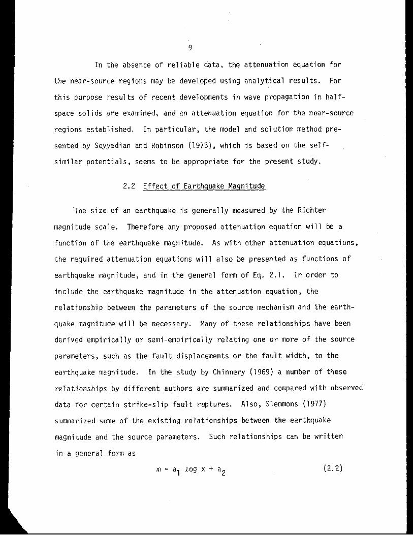
In the absence of reliable data, the attenuation equation for
the near-source regions may be developed using analytical results. For
this purpose results of recent developments in wave propagation in half
space solids are examined, and an attenuation equation for the near-source
regions established. In particular, the model and solution method pre
sented by Seyyedian and Robinson (1975), which is based on the self
similar potentials, seems to be appropriate for the present study.
2.2 Effect of Earthquake Magnitude
The size of an earthquake is generally measured by the Richter
magnitude scale. Therefore any proposed attenuation equation will be a
function of the earthquake magnitude. As with other attenuation equations,
the required attenuation equations will also be presented as functions of
earthquake magnitude, and in the general form of Eq. 2.1. In order to
include the earthquake magnitude in the attenuation equation, the
relationship between the parameters of the source mechanism and the earth
quake magnitude will be necessary. Many of these relationships have been
derived empirically or semi-empirically relating one or more of the source
parameters, such as the fault displacements or the fault width, to the
earthquake magnitude. In the study by Chinnery (1969) a number of these
relationships by different authors are summarized and compared with observed
data for certain strike-slip fault ruptures. Also, Slemmons (1977)
summarized some of the existing relationships between the earthquake
magnitude and the source parameters. Such relationships can be written
in a general form as
(2.2)
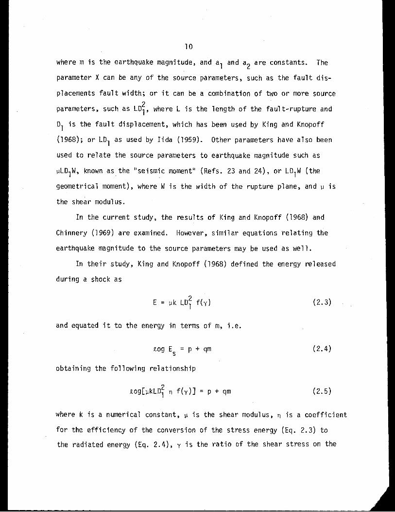
10
(2.5)
(2.3)
(2.4)
2E = 11k LDl f(y)
tog E = P + qms
during a shock as
and equated it to the energy in terms of m, i.e.
In the current study, the results of King and Knopoff (1968) and
Chinnery (1969) are examined. However, similar equations relating the
earthquake magnitude to the source parameters may be used as well.
In their study, King and Knopoff (1968) defined the energy released
for the efficiency of the conversion of the stress energy (Eq. 2.3) to
the radiated energy (Eq. 2.4), y is the ratio of the shear stress on the
obtaining the following relationship
where k is a numerical constant, 11 is the shear modulus, n is a coefficient
where m is the earthquake magnitude, and al and a2 are constants. The
parameter Xcan be any of the source parameters, such as the fault dis
placements fault width; or it can be a combination of two or more source
parameters, such as LD~, where L is the length of the fault-rupture and
Dl is the fault displacement, which has been used by King and Knopoff
(1968); or LDl as used by Iida (1959). Other parameters have also been
used to relate the source parameters to earthquake magnitude such as
11LD1W, known as the "seism~c moment" (Refs. 23 and 24), or LD1W (the
geometrical moment), where Wis the width of the rupture plane, and 11 is
the shear modulus.
11
(2.9)
(2.10)
(2.8)01 = exp (1.78m - 12.31)
m= 0.79 £og L01W - 4.74
m = 1.67 £og LW - 14.51
as
rupture surface after and before a shock (i.e. the stress drop), and
p and q are constants. Assuming an appropriate function for f(y), King
and Knopoff (1968) showed that Eq. 2.5 can be written in a general form
£og LO~ = 2.24m - 4.99 (2.7)
with n = 2 being an appropriate value for this relation. Based on observed
data, Eq. 2.6 is evaluated as (for 8.5 > m > 5.5)
The above equation can be written in a simpler form in terms of the fault
displacement only. This can be done by substituting the appropriate
equation relating L to the earthquake magnitude, e.g. L = exp (1.596m -7.56)
which is based on world-wide data. In this form, Eq. 2.7 becomes
where 01 is in meters.
Other equations, relating source parameters to the earthquake magnitude
are due to Chinnery (1969). Based on historical earthquake data for some
strike-slip fault movements, Chinnery has proposed a number of relationships
between source parameters and the earthquake magnitude. Among these, two
equations which are of importance to the present study are as follows.
These equations indicate the importance of combining different source

12
(2.11)
(2.12)
(2. 13a)
(2. 13b)
°WO. S= exp (2.47m - 15.97),
2
) a~ 2 a Ux(ic +]l -+ 1J V' u =P--2ax x at
2a~ 2 a u
(A + ]l) -- + ]l V' U = p --Y...ay y at2
In general, the problem of motion of a point at the ground surface
2.3 Wave Propagation in Half-Space Solids
parameters in determining their relationships with the earthquake magnitude.
Also, based on the data given by Chinnery and a statistical analysis, a
particular relation between m and 0lwO. 5 may be derived. This relationship
for m > 4 is shown in Fig. 2.1 and indicates a linear relation between m
and tog (0,wO. 5) as follows
or alternatively
where 01 = Dz is the fault displacement in meters and Wis in kilometers.
due to an earthquake of fault-rupture origin is a three-dimensional wave
propagation problem. In order to simplify the procedure, Seyyedian and
Robinson (1975) idealized the three-dimensional problem as two two
dimensional problems and solved the wave propagation equations on the basis
The wave propagation equations of small magnitude for a homogeneous,
isotropic solid can be written as
of the method of self-similar potentials. The solution method may be
summarized as follows.
where ~ is a scalar potential function, whereas wis a vector potential
function. The problem, then, involves finding the two potential function
~ and ~ in order to define the complete state of displacement at a given
point. To do this Seyyedian and Robinson (1975) considered the following
(2.13c)
(2.14)
(2.15)
(2.16)
(2. 17b)
(2.17a)
132
(A + ~)3L\ + ~ ,iu
a uzaz z
=pa 2t
aux au aut!.=_+-"'y+_Z
ax ay 3z
IT = grad ~ + curl ~
Applying Helmotz's theorem to the displacement vector U,
where x, y and z are cartesian coordinates, p is the mass density of the
solids, u , U , and u are the components of the displacement vector IT, tx Y z
is time, and A and ~ are the Lame constants. In Eqs. 2.13, L\ and also
the operator v2 are defined by the following expressions:
potenti a1 ~ for this case are zero.
shown that
(v2 1 a2- -d)~ = a
v2 ap
(v2 1 a2a- --)w =
i 3t2s
two-dimensional problems:
(i) Plain-Strain Problem -- This is the case corresponding to a
dip-slip motion (see Fig. 2.2). The x and y components of the vector
From Eqs. 2.13 and 2.16, it can be

(2.18)
14
where vp = ~ 2~)/p and Vs = I~/p are, respectively, the speeds of
the P- and S-waves, and ~z is the z-component of ~.
(ii) Antiplane problem -- This case corresponds to a strike-slip
motion. The displacement vector consists only of component Uz (see
Fig. 2.3). Combining Eqs. 2.13 and 2.16 we obtain
2 1 d2
(v - v2 -;t2) uz = as
The combination of the above two problems, therefore, defines the three
components of the displacement vector IT at a given point. For a general
case of a half-space solid, the above problems are solved in a complex
domain by considering: (i) the effect of reflected waves at the free
surface of the half-space; (ii) the boundary conditions at the free surface
and at the rupture surface; and (iii) the possibility of the formation
of a head-wave and the effect of head-wave disturbances when an S-wave
reaches the free surface.
The displacement components u ,u and u are given as the real partsx y z
of the complex functions u ,u and u , which are, in turn, functions ofx y zthe potential functions introduced earlier. Other assumptions and comments
with regard to this model are as follows:
(i) In the above two-dimensional problems, the length of the fault-
rupture is assumed to be infinite. This assumption seems to be reasonable
for the near-source region, since for major earthquakes (magnitude greater
than 5 or 6) and sites close to the fault, only that portion of the rupture
which is in the vicinity of the site has a dominant effect on the maximum
motion at the site; i.e. the contributions from the end portions of the
fault-rupture may be much less significant. Thus, the rupture may be
15
assumed to be infinitely extended on both sides of the focus. However,
for sites that are far from the earthquake source, this assumption would
be inadequate, as the three-dimensional effects become more important.
(ii) The different source parameters associated with this model
are as follows:
1. Parameters Ox and Dz--These are fault displacements in dip-slip
and strike-slip rupture, respectively, as shown in Figs. 2.2 and 2.3.
2. Geometrical dimensions--These parameters are shown in Figs. 2.2
and 2.3 and include the focal depth h (depth of earthquake source), angle y
representing the orientaiton of the rupture surface relative to the free
surface, and width of the rupture surface W.
3. Geological parameters--These parameters are the speed of the P
and S-waves which are, respectively, vp = I(A+2~)/p and vs = I~/p , and
also the speed of rupture propagation.
2.4 Acceleration, Velocity, and Oiselacement inVertical and Horizontal Motlons
The term "intensity" is used as a measure of the severity and de-
structiveness of the ground shaking at a site. By this definition, there
fore, the maximum ground acceleration (a), maximum velocity (v), maximum
displacement (d), or the Modified Merecalli scale (MM) are all measures
of ground motion intensity.
Seyyedian and Robinson (1975) developed their results in terms of
displacements at a given point on the surface. Although an attenuation
equation may be derived for maximum ground displacements, the maximum
acceleration is usually used as a measure of earthquake intensity for
engineering purposes. The maximum acceleration components ax' ay , and az

----------------------------------------
16
may be found by differentiating the respective displacement functions.
Alternatively, the maximum acceleration may be found using the ratios
via and ad/v2, in which a, v and d are, respectively, the maximum ground
acceleration, velocity and displacement. Newmark, Hall, and Mohraz (1973)
obtained values of via and ad/v2 for both horizontal and vertical earth-
quake on the basis of an extensive study of horizontal and vertical earth
quake spectra. Such results may be appropriate for converting the maximum
displacements to maximum acceleration at a point. In the present study the
average of the values proposed in Newmark, Hall, and Mohraz (1973), reproduced
in Tables 2.1 to 2.4, will be used for this purpose.
The analytical method of Seyyedian and Robinson (1975) yields the
maximum displacements components at a point; these may be given in non-
dimensional terms as dx/Ox' dy/Ox and dz/Oz ' where dx' dy and dz are the
respective maximum ground displacements in the x, y, and z directions, and
Ox and Oz are, r~spectively, the fault displacements in dip-slip and strike
slip. The corresponding accelerations are obtained using the intensity
ratios of Table 2.1 through 2.4 in terms ofax/Dx' ay/Dx and az/Oz , where
ax and ay
are the acceleration components in the vertical and horizontal
directions, respectively, in a dip-slip rupture; whereas az is the horizontal
component of acceleration in a strike-slip rupture. The variation of these
accelerations with the horizontal distance 0 of a point from an earthquake
source (epicentral distance) are examined in this section including the
effects of the individual source parameters.
17
2.S.1 The Strike-Slip Case
The two-dimensional problem in this case is an anti-plane problem
which results in the horizontal component of motion in the z direction.
The maximum acceleration is given as az/Dz in this case, which has units
of g/m.
Analytical results appear to show that intensity is not much affected
by a change in the material properties of the half-space; the variation of
az/Dz are mainly affected by the geometrical parameters such as the depth
of the focus, h, the angle of fault orientation, y, and the fault width W.
The specific effects of these parameters may be described as follows.
The Fault-Width W--The variation of az/Dz with 0 highly depends on W.
Typical results indicating this are shown in Figs. 2.4 and 2.S for a variable
Wand constants y and h (y = 90 0 and h = lS and 20 kilometers). It can be
seen that the dependence of az/Dz on Wis reduced for values of W/h close
to or equal to 1. This can also be seen in Fig. 2.6 where the variation
of az/Dz against Wfor h = 15 kilometers and y = 90 0 is shown. An
examination of the results of Figs. 2.4 through 2.6 shows that for values
of W< h, the effect of Won the intensity may be represented as WO. S;
whereas, for W> h, the intensity may be represented as independent of W.
The Focal Depth h--For a variable h and constants Wand y the variation
of az/Dz against 0 shows that for sites very close to an earthquake source,
the intensity increases with a decrease in the focal depth h; whereas,
for points with distances greater than about 10 kilometers from the source
(0 > 10 km.) the intensity decreases for a shallow source (see Figs. 2.7).
Fault Orientation y--The variation of az/Dz with 0 is shown in Figs. 2.8
for different fault orientations y. In particular, the effect of y on the
variation of a 10 with 0 is shown for W= 4 and h =15 (W < h). and W= 20z z
18
(w > h). It appears that with y = 900 the average effect of y would be
obtained. Also for points very close to the earthquake source, the
intensity becomes approximately independent of y.
A change in any of the source parameters, therefore will alter the
result for the intensity. This fact, perhaps, verifies the large scatter
observed in available historical data which have been used to establish
most existing attenuation equations. Thus, the effect of the source
parameters is important and must be included in any proposed attenuation
equation. In the present study, on the basis of above discussion, the
effect of the source parameters in the proposed attenuation equation
for a strike-slip case is considered.
1. The intensity depends on the fault width Wespecially for cases
where Wis smaller than h; this dependence is proportional to the square
root of the fault width. For cases in which Wis larger than h, the
intensity tends to be independent of the fault width.
2. The focal depth, h, has a decreasing effect on the intensity
at a point close to an earthquake source; and an increasing effect on
the intensity at a farther site (0 > 10 km). For cases in which h is
between 10 to 20 kilometers (common values for most earthquakes in
California) and for points close to the source, the intensity stays
approximately constant (see Figs. 2.7).
3. The proposed attenuation equation may be obtained for a specific
fault orientation; or the effect of y can be represented in the equation
by the average for all values of y. In the current study, the case at
which y = 900, i.e. vertical fault, will be considered.

-- --- -- ----
(2.20b)
(2.19a)
(2. 19b)
(2.20a)w<h
w<h
w>h
w>h
a /0 = 0.8 hl . 08 WO. 50 (0.7 0+h)-1.62z z
a /0 = 0.45 hl .08 WO. 50 R- l . 523z z
used:
where R is in kilometers.
of the S-wave; i.e. v /v = I(A+2~)/~. However, this effect is not veryp s
2.5.2 The Dip-Slip Case
19
half space as represented by the ratio of the speed of the P-wave to that
the results in this case are also affected by the type of material in the
This is the case corresponding to a plane-strain problem; and the
results are the displacements in the x and y directions (see Fig. 2.2).
The maximum acceleration components in this case are a /0 and a /0 .y x x xAgain, in this case, the variation of a /0 and a /0 with epicentraly x x xdistance 0 has been examined with regard to the effects of different
source parameters. Aside from the effects of the parameters W, handY,
?where az is the horizontal acceleration in g's, Oz is 'the fault displace-
ment in a strike-slip rupture, in meters, and W, h, and 0 are in kilometers.
Also, in terms of the focal distance, R, the following equations may be
Based on the above discussion, the following equations are proposed
for the horizontal motion in a strike-slip case.

20
(2.21)
These results show that the effect of Wis not very pronounced,
Effects on Horizontal Component a /D -- Figs. 2.9 and 2.10- y-x
variation of ay/Dx with epicentral distance Dfor different W.
values of hand y were used, with h = 15 and 20 kilometers, and
(i)
parameters may be summarized as follows.
Accordingly, the following equation is proposed:
attenuation equation may be obtained, using the average values obtained
where ay, the horizontal acceleration, is in gis, Dx in meters and 0
in kilometers.
especially at the close-in regions. Other parameters examined are the
with W=4 to 10 and h=lO to 25 kilometers, and a specific fault orientation.
focal depth, h, the ratio v /v , and the angle y. The results obtained. p s
in this case indicated that for points close to the source, the effects
show the
of the parameters h and v /v are also not very pronounced; these can bep sseen in Figs. 2.11 and 2.12. However, the intensity in this case depends
highly on the fault orientation y. The effect of y can be seen in Fig. 2.13,
where for the case of W=4 and h=15 kilometers the variation of a /D versusy x
D is shown. On the basis of the results described above, a suitable
(ii) Effects on Vertical Component ax/Ox -- The results for the
vertical acceleration, ax/Ox are shown in Figs. 2.14 to 2.18. The
parameter which affects a /0 significantly is, again, the rupture anglex xy (see Fig. 2.18). However, other parameters such as W, v /v and h
p s
Constant
y = 900.
significant on the y-component of motion. The effects of the various

21
(2.22a)
(2.22b)
= 17.3 WO. 80 (v Iv )-1.54°(0+15)-1.80P s
a 10 = 17.3 WO. 80 (2+A/~)-O. 77 (0+15)-1.80x x
The analytical results presented herein for both the horizontal and
vertical accelerations, show that the maximum ground motion at a given
1. The attenuation equation may be obtained by fitting a curve to
position. Here, an attenuation equation is presented for the case of a
vertically oriented rupture (y = 900 ).
epicentra1 distance from the source is a function of several parameters
to a greater degree than the corresponding effects on a 10. Based ony x
a detailed examination of the results for this case, the following are
Based on the above discussion, the following attenuation equation is
proposed for the vertical acceleration arising from earthquakes of dip-
of the source. In particular, the rupture angle y appears to have the
that part of the results corresponding to points close to the source.
2. The effect of the rupture width, W, and the ratio of wave
speeds, Vplvs' may be represented as WO. S and (VpIVs)-1.54.
3. The attenuation equation ought to be given explicitly as a
function of y; because of the irregularity in the effect of y (see
Fig. 2.18), a single parameter cannot represent the effect of the fault
or alternatively
suggested:
where a is in gis, 0 in meters and Wand 0 in kilometers.
slip origin.
(Figs. 2.14 through 2.17) also affect the vertical acceleration; generally

22
where 0 is the epicentra1 distance in kilometers, R is the focal distance
w<h (2.24a)
w>h (2.23b)
w>h (2.24b)
a = 3.6x10⁻⁶ h1. 58 e1. 78m (O.70+h)-1.62z
a = 2.02xlO-6 hl . 08 WO. 50 e1. 78m R- l . 523z
a = 2.02x10⁻⁶ hl . 58 el . 78m R- l . 523z
(ii) For Dip-slip
magnitude with the aid of Eqs. 2.8 through 2.12. After performing the
a = 5.59xlO-4 el . 78m (0+12.5)-1.95 (2.25)Y
a = 7.80xlO-5 WO. 8 (2+A/~)-O.77 el . 78m (0+15)-1.8 (2.26)x
az = 3.6x10⁻⁶ h1. 08 WO. 50 el . 78m (O.70+h)-1.62 w~h (2.23a)
largest effect on the maximum motion. Consequently, unless an attenuation
equation is expressed as a function of these parameters (particularly y),
it would not be surprising to see significant scatter in the observed
motions around the given attenuation equations.
The attenuation equations may be presented in terms of the earthquake
necessary calculations and replacing 01 by 0 or 0 wherever necessary,x zthe following equations ar~ obtained by virtue of Eq. 2.8.
(i) For strike-slip
and in terms of the focal distance R,
in kilometers, and ax' ay and az are maximum accelerations in gls.
region.
equations may then be obtained based on Eqs. 2.19 through 2.22 for that
(2.27)
(2.28)
a = 9.26xlO-8 hl .08 e2. 47m (O.7D+h)-1 .62z
a = 5.21xlO-8 hl . 08 e2. 47m R- l . 523z
and in terms of R,
2.6 Comparison with Existing Attenuation Equations
Eqs. 2.8 through 2.12 have been used here, other appropriate equations
Although, the magnitude-source parameters relations specified by
23
The proposed attenuation equations for the strike-slip case may
also be given in a simpler form and independent of the parameter W. This
can be done by applying Eq. 2.12, which relates D1WO. 5 to m, which yields
the following equations
is enough information available in a specific region, suitable attenuation
relating m to W, Dz or Dx may be used also to develop the attenuation
equations in terms of the earthquake magnitude. In this regard, if there
A number of existing attenuation equations proposed by different
authors are summarized in Table 2.5. In these equations the maximum
ground acceleration is given in terms of the magnitude m and distance R.
However, the distance R has different interpretations in different
equations. Comparison of results from these equations with those of the
present study has been made for a strike-slip motion and specific source
parameters appropriate for earthquakes in the Western United States.

24
Based on the data given by Chinnery (1969) regarding different
values of Wfor a number of important earthquakes in California, a W
equal to 5-6 kilometers will be used with Eqs. 2.23; also a depth, h,
equal to 20 kilometers will be considered. These values appear to be
equivalent to California earthquakes with magnitudes 6 ~ 7 in the Richter
scale. The epicentral distance is used here for the purpose of comparison.
Wherever necessary, a suitable transformation was made to define the
results in terms of epicentral distance. The results are then compared
with those proposed in the present study as described below.
Equations 2.23 and 2.27 are shown in Fig. 2.19 along with results
from the attenuation equations given in Table 2.5 for m = 7. As it can be
seen, for sites close to an earthquake source the equation by Donovan
(1974) gives lower values for maximum acceleration than the values from
the present study. For sites with D~ 10 kilometers, the situation is
reversed. Comparing with Esteva's equation (Ref. 17), it can be seen
that the maximum accelerations from the equations proposed in the current
study are generally higher. With regard to the equation by McGuire (1974)
a better agreement is observed; and as it can be seen in Fig. 2.19, for
sites close to the source, the ground accelerations predicted by the
present study are slightly higher than those obtained with McGuire's
equation. Finally the attenuation equation of Trifunac and Brady (1975),
with the appropriate values for the parameters in their model, is shown
in Fig. 2.19. In contrast to the attenuation equations of Donovan and
McGuire, results obtained with the Trifunac and Brady relation are
consistently higher than those of the present study. As it can be seen,
the difference becomes significant for sites that are close to the
earthquake source.

25
In summary, according to the present study, for California earthquakes,
the existing attenuation equations generally underestimate the ground
accelerations for close-in or near-source regions. However, this is not
always the case and a number of existing equations (e.g. that of Trifunac
and Brady) would consistently predict higher ground accelerations particu
larly at points close to the earthquake sources.
The differences in the calculated intensities based on different
attenuation equations (see Fig. 2.19) become critical in the design of
important structures, such as nuclear power plant; in the sense that some
of the attenuation equations may under-estimate the site intensities
whereas others may tend to over-estimate the true intensity at a site.

motions are not significant to engineering.
ate with distance such that at locations far from the breaks the ground
(3.1)S = exp(am-b);
3.1 Earth~ake Mechanism
26
CHAPTER 3
RELATIONSHIPS NEEDED IN SEISMICRISK ANALYSIS
The length, S, of the rupture zone is related to the total energy
released, to the type of fault, and to other geological and regional
tude, m. Such a relation can also be shown as
release of stored energy through the rupture of the earth's crust, along
lines or zones of weakness, known as "faults." The point where the rupture
factors and may be several hundred kilometers long for a large-magnitude
earthquake. Generally, a linear relationship between magnitude and the
logarithm of the fault length is given to relate s to the Ricter magni-
Most earthquakes of significance to engineering are believed to be
of tectonic origin. A tectonic earthquake is the result of the sudden
of rupture, but at any given instant the earthquake origin would lie in
a small volume of the crust (practically a point) and would travel along
the fault (Ref. 39). The intensity of the earthquake shocks will attenu-
quake, a chain reaction would take place along the entire length or area
first occurs is the focus of the earthquake. In a strong-motion earth-
where a and b are constants. For example, based on world-wide data,

27
3.2 Earthquake Magnitude and Slip Length
(3.3)
(3.2)
log N(m) = p - qm
s = exp(l .596m - 7.56)
Based on the Richter's law of earthquake magnitude, the probability
density function of magnitude, i.e. fM(m), may be derived. According to
this law, in a certain zone of the crust and during a given period of time,
the occurrence of earthquakes can be approximated by the relationship
where N(m) is the number of occurrences with magnitude m or greater, and
p and q are constants (Richter, 1958). Alternatively, Eq. 3.3 can be
Despite the large uncertainty in the rupture length-magnitude re
lationship, such relationships are useful for seismic risk analyses.
It has been shown by Der-Kiureghian and Ang (1975) that the effect of
this uncertainty is much less than that from the uncertainty in the
attentuation equation.
Equations similar to Eq. 3.2 may also be derived based onfue study
of the availabel data for a specific region. Due to the smaller scatter,
which is expected for data available in a specific region, the correspond
ing rupture length-magnitude relation, therefore, involves less uncertainty.
However, such relations are not available for many regions because of the
lack of adequate data.
Eq. 3.1 is evaluated to be

28
(3.5)
(3.7)
(3.4)
(3.6)m < m < mo - u
el sewhere
-8(m-mo)() 1 - eF
Mm = --'--"----,----..,....
-8(m -m )1 _ e u 0
fM(m) = t exp[-8(m-mo)];
= a
In the seismic risk analysis of lifeline systems, sometimes it is
Considering a lower bound magnitude, mo' and an upper bound magnitude,
mu
' it can be shown that the cumulative distribution function of magnitude
may be derived from Eq. 3.4 in the following form:
N(m) = exp(a - 8m)
The corresponding probability density function will, then, be
where a = 2.3p and 8 = 2.3q.
more convenient to use the probability density function of rupture length,
written in the following form:
s, instead of that of earthquake magnitude, m. The probability density
function of s can be easily obtained from Eq. 3.6 by considering the re-
which is in the form of a shifted exponential distribution function with
constant k being equal to

Substituting Eqs. 3.6 and 3.9 in Eq. 3.8 and carrying out the differentia-
(3.11)
(3.13)
(3.12)
(3.10)
(3.9)
(3.8)
s < s < so - - u
elsewhere
c = Sa(s -s/a s -s/a)
o u
Su = exp(amu - b);
So = exp(amo - b);
- 1 )g (s = m = [In(s) - b]/a
-(s/a + 1)fS(s) = c s
= 0
where rupture 1ength So and Su correspond to the lower-bound and upper
bound magnitudes, respectively.
and
in which
where g-l(s) is the inverse of function s = g(m), i.e.
tion, the probability density function of s becomes
29
lationship between m and s (EC]. 3.1) and the following general equation
- ------------
30
In the study by Der-Kiureghian and Ang (1975,1977), the influences
of parameters mo and mu and S on the calculated risk were examined.
Among the major conclusions are the following:
(i) The parameter S, which is the slope of the magnitude-recurrence
curve (Eq. 3.3), should be chosen carefully for a region, since the calcu
lated probabilities are sensitive to this parameter.
(ii) The lower-bound magnitude mo should be such that earthquakes of
magnitudes equal to mo and smaller do not produce damaging intensities.
Generally, a value of mo = 4 is appropriate.
(iii) The upper-bound magnitude mu need not be greater than 9.
Even if earthquakes of magnitude greater than 9 are possible, the contri
butions to the calculated risk would not be significant.
3.3 Modeling Potential Earthquake Sources
As discussed earlier, geologic faults are believed to be the main
potential sources of destructive earthquakes. However. for many regions,
the fault system may not be known or well surveyed. For this reason, in
order to permit the modeling of all conceivable seismic sources, three
types of idealized models are introduced and will be used in the evaluation
of the earthquake hazards to lifeline systems. These seismic sources are
designated as Types 1, 2, and 3 and defined respectively as follows:
(i) Type 1 Source--A well-defined fault or fault system. The length,
direction, and position of the fault relative to the site are assumed to be
known in this case. This model would be appropriate if the potential seis
mic activity is expected from a well-defined fault or fault system. such as
the San Andreas fault in California.

31
(ii) Type 2 Source--Fault direction known. The exact location of a
fault with respect to a site is not known, but the dominant orientation of
the fault or fault system is known. This case would arise when a certain
zone of the crust contains numerous active faults with a common orienta
tion, or where the location of the fault-rupture may occur in a dominant
direction.
(iii) Type 3 Source--Unknown faults. The fault location as well as
their directions are unknown. This model is appropriate for modeling of
those areas in which a potential zone of the crust contains numerous active
faults with no dominant direction, or the locations and the orientations
of the faults are completely unknown.
In order to model the fault system in a region of seismic activity,
one or more of the three types of seismic source models, as described
above, may be used. In the following chapters, the calculation of the
risk for all three types are introduced and described. In all cases, the
effect of rupture length is included in this study.

32
CHAPTER 4
MODELS FOR SEISMIC HAZARDANALYSIS OF LIFELINE SYSTEMS
4. 1 Introductory Remarks
A lifeline system is composed of a number of elements (e.g. pipelines,
segments of a highway) linked together to carry out a certain level of
service for the benefit of the public. Simple lifeline networks, as
shown in Fig. 4~1, consist of several links in series or parallel, with
an entry point and a final point. In a water distribution system, the
entry point is usually a water supply station, whereas the final point
can be any point for which water is needed. The objective in this system
is to maintain the flow of water from the water supply to any given point
in the system. Large lifeline systems cover vast spatial areas and are
composed of links each of which may be several kilometers long. In
general the objective in a lifeline system is to maintain the flow of a
certain quantity, such as water in the case of a water distribution system;
or the flow of traffic in the case of a transportation network, between any
two points of the system.
The purpose of seismic risk analysis of a lifeline system is to
evaluate the reliability of the system against earthquake hazards to carry
out its objective. The results of such analysis will be useful in the
design and planning of a lifeline system in a region of potential earth-
quake activity.
Aside from the potential for seismic damage caused by the strong
shaking of the ground, a lifeline system may also be subjected to the

33
This case concerns the possibility that during an earthquake the
(4.1)v.1
nv = I
i=l
Suppose that in a region, n potential earthquake sources were
Given an earthquake with origin (hypocenter) located at source i,
the probability of a fault-rupture strike on a given link j is P(L}IE i ),
4.2 Fault-Rupture Hazard
In this chapter the methods for evaluating the probabilities of
mode of failure is especially important in regions where shallow-focus
identified. If the average number of earthquakes per year with magnitude
greater than or equal to m in the i th source is v., the average numbero 1
of earthquakes in a year for the entire region then will be
presented for individual links. The respective probabilities of failure
permit modeling of all possible potential sources in the region.
earthquakes are likely to occur, such as the Western United States.
are possible.
lifeline system and, therefore, will cause the failure of the links. This
possibility of a fault-rupture strike on one or more links of the system.
rupture, initiating at the focus, will strike one or more links of a
of the system involves a detailed correlation analysis which is described
encountering either of the above two modes of earthquake hazards are
This case is particularly of concern in the regions where surface ruptures
in the next chapter. In the evaluation of probabilities in both modes of
failure, the three types of source models will be considered in order to
34
(4.3)
(4.2a)
(4.2b)
(4.2c)
-n. P(L.)J
U L~rJ
P(L~ E.) P(E.)]J 1 1
= 1 - P([~ [~ ~ )J J J
n= 1 - 1T [1
i=l
\).
= -'\)
P(L.) = 1 P([~) P([~)J J J
nP(L
J.) ~ I P(L . IE.) P(Ei )
i=l J'
P(E i )
j becomes
Assuming the average occurrence rate in source i relative to that
in which L~ = a rupture strike on link j due to an earthquake in source iJ
and Ei is the occurrence of an earthquake in source i. Thus the probability
of a fault-rupture strike on link j due to an earthquake in the i th
source is P(L~) = P(L~IE.) P(E.). Considering n potential earthquakeJ J 1 1
sources in the region, the probability of a fault-rupture strike on link
-iwhere Lj is the event of no fault-rupture strike on link j due to an
earthquake in source i. It is reasonable to assume that L~ are statisticallyJ
independent; hence,
For small probabilities, P(L~ E.) and P(E.), Eq. 4.2b can be given as,J 1 1
where the superscript i is dropped for simplicity.
over the entire region remains constant with time, the probability of
occurrence of the event Ei may be expressed as,
35
Substituting Eq. 4.3 in Eq. 4.2c,
Poisson process is an acceptable and useful occurrence model in seismic
(4.5)
(4.4)
(4.6)
1 n= - I P(L·IE.) v.
Vi=l J 1 1
nP(L.) =l-exp[- I P( IE) ]J one yea r . 1 L. . v. •
1= J 1 1
nP(L.) = I P(L./E.) v.
J one year i=l J 1 1
n v.P(L.) = L P(L.IE.) 1
J i=l J 1 v
The Poisson process, which assumes temporal and spatial independence
The future occurrence of earthquakes in a region may be assumed to
constitute a homogeneous Poisson process, with the average occurrence
rate v per year. During each occurrence, there is a constant probability
of fault-rupture strike on link j; it follows then that the occurrence ofn
a Poisson process with activity rate v P(LJ.) or I P(L.IE.) v ..
i=l J 1 1
the probability of a fault rupture strike on link j in one year
is
L. is alsoJ
Therefore,
For small values of this probability (cases of practical interest)
the above result can be approximated by
of earthquake events, may not be consistent with the elastic rebound
theory of earthquakes; and this process is unable to portray earthquakes
as the release of gradually accumulated strains in the earth's crust or to
describe foreshocks and aftershocks. In spite of these shortcomings, the
36
risk analysis, especially for moderate and large earthquakes (Rosenblueth,
1973).
From the above formulations, it can be observed that the main task
involves the determination of the conditional probability P(LjIEi). This
conditional probability will depend on the three idealized types of
sources, described earlier.
4.3 Determination of P(L. IE.)J..1....'::.,-
The term P(LjIEi) is defined as the probability of a fault-rupture
strike on link j of a lifeline system, given an occurrence of an earth
quake in source i. The magnitude and location of this earthquake within
source i is random. In general the following are assumed.
i. The random magnitude of a given earthquake has the density
function given by Eq. 3.6. Alternatively it may be defined that the
random rupture length of a given earthquake has the density function
given by Eq. 3.10.
ii. The distribution of the focal location is uniform over the
source.
iii. An earthquake originates as a rupture propagating symmetrically
on each side of the focus along the fault. The length of the fault
rupture (slip) is related to the random magnitude through Eq. 3.1.
On the basis of above assumptions, the methods to evaluate the
conditional probability P(LjIEi) for each of the three source types are
as foll ows.

or
(4.9)
(4.7)P(L. IE.) = JP(L ·1 E. ) f S(s) ds;J 1 '1., J 1,S
s/ Q,; if 5/2 ~ °~ ° (4.8a)
P{L.!E. ) = (5/2+°1 )/ if D ~ s/2 < ° (4.8b)J 1, S
O. ; otherwise (4.8c)
Using the results of Eqs. 4.8 in Eq. 4.7 and carrying out the integration,
the conditional probability P{LjIEi) becomes
201 s2
Js ( s+201
P{LjIE i ) = i fS{s)ds + 2'1.,
So 20i
For an earthquake with magnitude m from a Type 1 source, the
conditional probability P{LjIEi) can be written as
where E. = an earthquake in source i with rupture length s in which1 ,S
S = exp{am-b); and '1., indicates the length of the fault.
Denoting 01 and O2, respectively, as distances from the intersection
point to link j with the fault to the nearest and farthest ends of the
fault, as shown in Fig. 4.2, and considering that the rupture is extended
by s/2 at each side of the focus, the conditional probability P{L.IE. )J 1, S
can be obtained in terms of s, Q, and Dl . It is observed that:
If O2 ~ Q" with uniform probability distribution along the fault,
we have
374.3.1 Jype 1 Source (Well-defined faults system)

(4.llb)
(4.l1a)
(4.1 Ob)
(4.10c)
(4.10a)
- - -----------------~
otherwi se.0;
38
= c [(20l
)1-B/a + s2l-B/a-2S0l-B/aJ2dl-B/a)
cOla -o/a 01- ---- [s p - (201
)-P a];9,13 2
= c [l-B/a l-S/aJ2£(1-s/a) s2 -so
cD a+ 1_ [s-B/a _ (20 )-B/a J9,13 2 1
----------------
P(l·IE.)J 1
P(l·IE.)J 1
p(l·lE. ) =J 1, S
( I ) - c 1-sla )1- 131 aP lj Ei - 29,(1-B/a) [s2 -(201 ]
Similarly if O2 > 9, ,
where s2 = the smaller of 202 and suo
For certain exceptional cases So may become larger than 201, in
which case 201 in Eq. 4. lOa should be replaced by So and therefore,
Eq. 4.10a becomes
Substituting Eqs. 4.11 in 4.7 and performing the integration, the
conditional prObability P(ljIEi ) becomes

39
(4.13)
(4.12)
occurrences within ~Ai per year t vi may be obtained directly.
For an earthquake of magnitude m in the ith source (~Ai)' the rupture
will extend s/2 at each side of the focus parallel to ox direction. De
noting D as the distance from ~Ai with the link jt in this case the rupture
will strike link j only if s/2 is greater than D. Therefore t the conditional
probability P{Lj/Ei ) in this case
Consider a seismically active zone of the earth's crust as shown in
(i) Assume uniform activity rate over A; then
where vA is the activity rate for area A.
(ii) From statistical data t i.e. the average number of earthquake
By dividing the shaded area t Alt into smaller areas ~Ai with coordi
nates x and y with respect to axes ox and 0Yt each ~Ai can be considered
as a single source with occurrence rate vi which can be defined in either
of the following ways.
earthquake of magnitude m occurs within the shaded area t Alt shown in
Fig. 4.3.
by ox making an angle a with respect to link j. In this case t reference
Fig. 4.3 denoted by A. The dominant direction of the faults is denoted
to Fig. 4.3 will show that a fault-rupture strike will occur only if an
4.3.2 ~2 Source (Dominant fault direction known)
40
(4.16)
(4.15)
(4.14)
P(L·IE. m) fM(m)dmJ "
p(L·IE.)J ,
The seismically active area, A, is again divided into smaller areas
As shown in Fig. 4.4, for an earthquake of magnitude m originating in
~Ai' the possible positions of a fault-rupture will form a circular area
with diameter s. The rupture will strike the link j when the circle inter
sects the link. From the total probability theorem, the conditional proba
bility P(LjIEi) can be shown to be,
in the region is not uniform, vi can be obtained directly from statistical
data.
~Ai each of which considered as a single potential source with an occur
rence rate equal to vi. Also in this case, if the seismic activity appears
to be uniform over an area A, the occurrence rate vi for the ith source
within the area can be obtained from Eq. 4.12; whereas if the seismicity
m1 = [In(2D) + bJ/a
For a type 3 source, an earthquake may occur anywhere in an area,
and the fault-rupture may propagate in any direction with equal probability;
i.e. uniformly distributed in (O,2n).
o = Ix-y tan(a)!
4.3.3 Type 3 Source (Unknown faults)
and
where,

41
llds
(4 .18b)
(4.18a)
(4.17)p(L·IE. ) = ~J 1 ,m 1T
1p(L·IE.) --J 1 1T
mufM(m) + f
m3
Note that e is a function of s and, therefore, a function of m.
ml is the larger of mi and mo' where m' is found from the condition
D= s/2, or equivalently
where x and yare the coordinates of small area ~Ai' s = exp(am-b), and
£j is the length of link j.
The magnitudes ml , m2 and m3 are found from the governing conditions,
given in Table 4.1 as follows:
in Table 4.1.
rupture s; the different cases and corresponding values of e are summarized
Substituting els from Table 4.1 in Eq. 4.18a we obtain"
The value of e in Eq. 4.18 depends on the distance D and the length of the
Therefore, Eq. 4.16 becomes
where Ei,m = the occurrence of an earthquake in source i with magnitude m.
Denoting e as the agn1e of intersection of the circle with diameter sand
1ink j, it appears that
cas~s:
The following modification may be necessary for certain exceptional
(4.19)
(4.20)
(4.21 )
42
[In(20) +b]/aml
1
m2 = [In(20 ' ) + b]/a
m3 = [In(20") +b]/a
m2 is found from the condition 0' = s/2 or
where 0 = the closest distance between link j and bA ..1
where 01 = distance from AAi to the nearest end of the link.
m3 is found from the condition Oil = s/2 or
where Oil = distance from bAi to the farthest end of the 1ink.
Once m1, m2 and m3 are found from Eqs. 4.19 to 4.21, P(LjIEi) can
be evaluated numerically from Eq. 4.18b.
For sources that are far from the link, m may be larger than mu' In
such cases P(LjIEi) = 0; whereas for sources that are very close to link j,
o may be equal to zero and, therefore, P(LjIEi) = 1.
The choice of the dimensions of bAi should depend on the distance from
the link. On the basis of a number of example problems analyzed, it appears
that for sources with distances up to 20 kilometers from the link, bAi = 1.5
to 2 sq. kilometers is adequate and for farther sources bAi may be increased
gradually.

43
v. ,1
(4.24a)
(4.23)
(4.22)
P(Y>y E.) v· .r 1 1
n= 1-exp [1- I P(Y>YrIEi)vi ]
i=l
P(Y>y IE.) P(E.)r 1 1
nI
i=l
nI
i=l
1= -v
P(Y>y )r one year
P(Y>y )r
Again, assuming a homogeneous Poisson process, with activity rate
for the occurrence of future earthquakes, Eq. 4.23 becomes
4.4 Hazard from Severe Ground Shaking
This mode concerns the maximum ground motion intensity exceeing
where Y is the maximum intensity (from n potential sources) at a point
along the link j; and E. is the occurrence of an earthquake in source i.1
Using Eq. 4.3, Eq. 4.22 becomes (Der-Kiureghian and Ang, 1977)
a common material and the same fabrication process are used in construction
of a link may be assumed to be at the point of maximum ground motion along
the link. If there are n potential earthquake sources in a region, then
the probability that the maximum ground motion will exceed some specified
intensity Yr at any point along a link,
a lifeline system, it is reasonable to assume that the resistances along
a link are perfectly correlated, even though the correlation between any
two links may be weak. On this basis, the location of potential failure
the resistance capacity of one or more links in a lifeline system. If
44
(4.24b)
(4.25)
p(Y> y IE.) \!. •r 1 1
nI
i=lp(Y> y ) -
r one year
P(Y>y IE.)r 1
Type 2 source model--appropriate for earthquake sources originating
Type 1 source model--appropriate for modeling potential sources origi-
Type 3 source model--appropriate for modeling regions or areas in which
Eq. 4.25 must be evaluated for all potential sources in the region.
The main problem, therefore, involves the determination of the con-
ditional probability P(Y>y IE.). From the total probability theorem,r 1
Essentially, the three types of source models of Der-Kiureghian and
Ang (1977) are similar to those described earlier for fault-rupture hazard;
and for small probabilities
this can be evaluated as
namely:
permit the modeling of all conceivable seismic sources. These have been
developed by Der-Kiureghian and Ang (1977), and may be used to evaluate
the hazard to the present mode of failure of a lifeline system.
nating from well-defined faults;
the fault system is not known.
In this case, also, three types of source models are necessary in order to
in areas where the fault locations are not known, but the dominant orienta-
tion of the fault system is known; and
where E. = the occurrence of an earthquake with magnitude m somewhere in1,m
source i.

45
4.5 Critical Section of a Link
As indicated earlier, under quite reasonable assumptions, the safety
of a lifeline system to the hazard of high-intensity motions may be con
fined to the consideration of the critical section of each link, where the
probability of exceedance is the highest along the link. The location of
the critical section along a given link, however, may not be determined a
priori. In general, the probabil ity of exceedance for several points along
a link may have to be calculated, considering the effects from all n
potential earthquake sources in the region. The point corresponding to the
highest probability, under the assumptions indicated earlier, determines
the critical section along the link.
The number of points for which the probabilities of exceedance may
have to be calculated along link j will depend on the length of the link
and its location relative to the potential sources in the region. On the
basis of a number of example problems analyzed, it appears that for most
cases, the critical section is located at either ends of a link; however,
this is not always the case, especially for links that are quite long
(e.g. > 20 kilometers).

46
CHAPTER 5
SEISMIC SAFETY EVALUATION OFLI FELINE SYSTEMS
5.1 Probability of Failure of a Link
The methods introduced and presented in the previous chapter
provides information about the probability of a fault-rupture strike
on a link and the probability that the ground motion intensity will
exceed the resistance capacity of a link in a lifeline system. This
information is needed to evaluate the probability of failure of a
given link as described below.
In the case of fault-rupture strike, the occurrence of such an
event for a given link would be tantamount to the complete failure of
the link. Therefore, the occurrence of a fault-rupture strike, as
described in Chapter 4, is also the probability of failure of the link.
For the severe ground motion hazard, the resistance of a link
relative to the maximum motion-induced force or strain must be con-
sidered in evaluating its probability of failure. More precisely, in
this case, convolution of the probabilities associated with all possible
values of resistance and maximum ground moiton will be necessary. The
annual probabilities of exceeding given levels of ground moiton intensities
may be obtained by using the method given in Chapter 4. Such probabilities
for different intensities may be portrayed graphically as shown in Fig. 5.1,
whereas the probability distribution of the resistance of a link may be
described with the probability density function (PDF) of Fig. 5.2. The
annual probability of a link failure (caused by high ground moiton), there-

(5.3)
(5.1)
(5.2)
t-.yFR(Yr - 2r ) is the probability that the
00
00
47
resistance will be in a small interval t-.Yr' as presented by the incremental
area shown in Fig. 5.2.
The probability distribution for the resistance R may be predicted to
be lognormal (Newmark, 1974). Therefore,
where FR(r) = the probability distribution function of intensity resistance,
and fy(y) = the probability density function of ground motion intensity.
However, for the present study, Eq. 5.1 is preferred over Eq. 5.2 as the
ordinates of the curve in Fig. 5.1 gives directly [l-FY(Yr)]'
Numerically, Eq. 5.1 can be evaluated as
of 1ink j is
where PF
. = the annual failure probability of a link, such as j; Yr is anJ
intensity level of ground shaking corresponding to the resistance capacity
of link j, and l-FY(Yr) is the exceedance probability of ground motion
intensity as given by the curve of Fig. 5.1.
An alternative but equivalent expression for the failure probability
fore, may be calculated from

Available data, of course, must be used in assessing Q. However, since
(5.5)
--------------_._-------
48
in whi ch </> (x) is the standard normal probabil ity, and ,
5.2 System Failure Probability
where Yr is the mean intensity resistance; and Q is the coefficient of
variation representing the uncertainty in the resistance of link j.
The coefficient of variation, Q, represents the degree of uncertainty
underlying the prediction of the resistance of link j. This must include
all the uncertainties underlying the predicted or estimated resistance for
the link. Therefore, the determination of the various sources of uncer
tainty associated with the prediction of the resistance is, perhaps, the
most important task in the evaluation of the safety of a lifeline system.
available data may not be sufficient to provide completely objective bases
for assessing the underlying degree of uncertainty, this may be augmented
with engineering judgments. The necessary judgments, however, may have to
be expressed in probability terms in order to derive the appropriate co
efficient of variation (Ang and Newmark, 1977).
The failure probabilities described above applies to individual
links, where FR(Yr) is evaluated for suitable increment of Yr' The
failure probability (in either mode of failure) of individual links
comprise the information necessary to determine the respective probability
of failure of a complete lifeline system.
------------------------------------------

· 49
In a simple lifeline system of links in series, the failure of any
link in the system will cause the complete failure of the entire system.
The problem becomes much more complicated in the case of a real lifeline
(5.6)
n.1
PF. = 1 - II1 j=l
system. In this case the failure of any possible path between the entry
point and the final point must be considered, taking into account the effect
of possible correlations between the different paths.
where n. is the number of links (in series) in path II.; PF = the1 1 •
Jprobability of the jth link in path 7T i in either mode of failure; and
PF. is the probability of failure of path 7T i (in any of the two modes1
of fa i 1ure) .
In this form, the network shows all possible paths to the final point
from the entry point in the lifeline system (see Fig. 5.3).
Assume that a lifeline system, after transformation, is composed of
5.2.1 Topological Transformation of a Lifeline System
For the purpose of evaluatingits failure probability, a lifeline
system may be modeled topologically as a network of parallel "paths" each
of which is composed of several links in a series (Shinozuka et al, 1978).
N parallel paths; and the ith path is ni links in series. If the failure
of a link in a path, such as TI i, is assumed to be satistically independent
from the failure of other links in the same path, the probability of fail
ure of path 7T. in the system wi 11, then be1
50
5.2.2 The Method of PNET
(5.7)
This correlation can be shown to be
0.0.1 J
and TIj.2I Ok
ks( TI i TI.)= __,--..><.J_
p •.lJ
any two paths TI i
of a path, such as TI i , is
-where ok = the standard deviation of those links that are common to paths
TI i and TIj; and 0i and OJ are, respectively, standard deviations of paths
TIi and TIj . If standard deviations for all links are equal (e.g. ° for
each link), and assuming statistical independence t the standard deviation
of lifeline systems.
The correlation between paths can be calculated by assigning a
standard deviation to each link. Such standard deviation is only for
the purpose of determining the correlation coefficient t Pij' between
links, as indicated earlier, may be uncorrelated. Such correlations be-
The failure probability of a complete lifeline system is much more
complicated in the sense that some paths have links in common and, for
this reason, are partially correlated, even though the failures of the
tween the path could be significant in the evaluation of the failure
probability of the entire system. In order to include the effects of such
correlations, the method of PNET (Ang, Abdelnour and Chaker, 1975) is
appropriate. The probabilistic network evaluation technique (PNET) has
. been previously developed for the analysis of activity networks (Ref. 3).
The technique is applicable also for the approximate analysis of safety
51
(5.10)
(5.9)nk
Pi j = --=-=-In. n.
1 J
where, r stands for the representative paths.
(5.8)
system, PF, is approximated as
The demarcating correlation Po' which defines the transition between
high and low correlations, has been previously taken as 0.5 in the analysis
with their mutual correlations as evaluated in Eq. 5.9, such that with
in each group the paths are mutually highly correlated. Therefore, the
paths within each group can be "represented" by the single path having
the highest probability of failure in the group, i.e. max(P F.); whereas,1
the "representative" paths between the different groups may be assumed to
be statistically independent. Then the failure probability of the complete
this basis, the paths can be divided into several groups in accordance
The PNET method, applied to the system failure probability of a
complete lifeline system, is based on the premise that those paths
that are hi gh ly correlated (e. g. with Pij > po) may be assumed to be per
fectly correlated; whereas, those with low correlations (i .e. Pij 2.Po)
may be assumed to be statistically independent (Ang, et al, 1975). On
where n. = the number of links in path TI.. If there are nk links in1 1
common to paths TI i and TI j , Eq. 5.7 becomes

52
of activity networks (Ang et al, 1975). For the purpose of the present
study, the same value, i.e. p = 0.5, appears to be also appropriate ando
will be used.
In order to examine the adequacy of the method of PNET, evaluating
the probability of failure of lifeline systems, a number of example problems
were analyzed also with Monte Carlo simulations. All possible combinations
of links, in a lifeline system, which cause the failure of the entire system
were considered. Using the failure probabilities of individual links,
the probability of failure of the entire system was obtained by the method
of Monte Carlo. In both modes of failure, the adequacy of the PNET was
confirmed.

53
CHAPTER 6
NUMERICAL ILLUSTRATIONS
6.1 Introductory Remarks
In order to demonstrate the applicability of the methods developed
and introduced in the previous chapters, the seismic safety analyses of
two different lifeline systems were performed. The first one is for the
water distribution system in the city of Tokyo, Japan. The seismic
hazard of this system to ground motion intensities has been examined
previously by Shinozuka, et a1 (1978). The second analysis is for the
highway network around Boston, t~assachusetts. For this latter network,
the seismic hazard to ground shaking has been analyzed as an example
problem in Ref. 49. In order to compare the results of the present study
with those of Refs. 47 and 49, where appropriate, the same parameters in
Ref. 47 and 49 will be used with the present study.
6.2 Seismic Safety Analysis of WaterDistribution System in Tokyo, Japan
The water for the city of Tokyo is supplied through a network of
pipelines from three supply stations A, Band C as shown in Fig. 6.1.
The system consists of twenty three links and fourteen nodes including the
three supply stations A, Band C. For the prupose of the present analysis,
the pipelines are idealized to consist of straight segments (dash lines)
as shown in Fig. 6.1. In this idealized form, the network is composed of
thirty two 1inks and twenty two nodes. In this problem the re1 iabi1ity of
the system to maintain the water flow from each of the three supply stations
to point 9 against ground shaking is studied.

at point 9; these annular areas are as follows.
54
Radius (km)
10.
40.
90.
160.
250.
1
2
3
4
5
Annul ar Area
The entire area is divided into five annular areas with a common center
based on the data available for this area, the entire region may be
Records of past earthquakes within 300 kilometers from Tokyo and with
magnitudes of 4 and greater are given in Refs. 28 and 47. An area with
In this example problem, an attenuation equation in the form of-b
y = bl (R+b4) 3 exp(b2m) is used with bl = 1.1, b2 = 0.5, b3 = 1.32, and
b4 = 25. However, any other attenuation equation that may be appro
priate for the Tokyo bay region may be used instead.
a 300-kilometer radius from Tokyo is considered for the analysis. Also,
6.2.1 Seismic Parameters and Sources forTokyo Bay Area
The epicenter map of the Tokyo bay area is shown in Fig. 6.2.
modeled as Type 3 sources.
The magnitude-recurrence curve is shown in Fig. 6.3; on this basis,
an occurrence rate equal to 3.6xlO-4 per year per square kilometer and
values a = 1.576, and b = 7.560, which are values based on world-wide
a slope B = 1.94 are obtained. Furthermore, for the Tokyo bay region
mo = 4.0, and mu = 8.0 appear to be reasonable. Also, in the absence of
information that may be more appropriate for the Tokyo bay area, the
data, will be used in the rupture length-magnitude relation.

55
Finally, an average depth, h, equal to 25 kilometers is assumed for
the entire area. The assumed average depth is only for the purpose of
illustration of the methods given herein; and in areas such as Tokyo,
where earthquakes of deep-focus are likely to occur, the average depth may
have to be revised based on information regarding the history of the im
portant earthquakes in the region.
6.2.2 Failure Probabilities of LinksDue to Severe Ground Motions
It is assumed that the intensity resistance of each link follows a
log-normal density function with a mean Yr and a coefficnet of variation Q.
In this example problem, different mean resistances ranging from 0.15g
to 0.6g are considered. Furthremore, a coefficient of variation equal to
20% is assumed. The assumed coefficient of variation is, again, for the
purpose of illustration and for a better estimation of the risk the
coefficient of variation must be evaluated based on available data and
engineering judgments in probability terms (Ang and Newmark, 1977).
Based on above assumptions, the risk, i.e. probability of failure due
to the ground shaking, is calculated for all links indicated in Fig. 6.1.
6.2.3 System Failure Probability
The risk associated with the failure of individual links in the second
mode of failure is the basic information necessary for the calculation of
the system failure probability. As shown in Fig. 6.4, the system is modeled
topologically as networks of parallel paths with links in series. The
failure probability of paths 1 to 14 (numbered from top to bottom) are cal
culated; the results are given in Table 6.1. Applying the method of PNET,
the effect of correlations between paths can be included in the calculation
of the failure probability of the complete lifeline system.
56
The paths in each of the networks A-to-9 and B-to-9 are arranged in
order of decreasing failure probabilities. The correlation coefficient
between path 2 (with largest failure probability in the network A-to-9) and
other paths, i.e. paths 1, 3 and 4, are P2,1 = .29, P2,3 = .33, and 02,4 = o.
Similarly for the remaining paths the correlation coefficient are Pl,3 = .29
and 01,4 = .57. Only path 4 ( 01,4 larger than 0.5) can be represented by
path 1; and, therefore, the representative paths in the network A-to-9 are
paths 1, 2 and 3. The network failure probability for the case Yr = 0.15g,
then, can be approximated as
PF (A-to-9) = 3.33 x 10- 3
Similarly, for the network B-to-9, the paths are arranged in order of
decreasing probabilities; the correlation coefficients in this case are:
P5,6 = .67, P5,7 = .8, P5,10 = P5,8 = .63, P5,9 = .47, P5,13 = .43, 05,12 = .41,
and P5,11 = .35. It appears that paths 6, 7, 10, and 8 are represented by
path 5. Similarly, 09,13 = .33, P9 ,11 = .45, P9,12 = .0, and 013,11 = .61,
P13,12 = .24. Therefore, the failure probability of the network B-to-9 is
represented by the failure probabilities of paths 5,12, 13, and 9, i.e. for
the case Yr = 0.15 g,
-3PF(B-to-9) = 1.21 x 10
The similar procedure is repeated for other mean resistances. The
final results--the probabilities of failure given in Table 6.2 and por-
trayed graphically in Figs. 6.5 and 6.6.
57
6.3 Seismic Safety Analysis of theNetwork of Boston Highways
Major highways around Boston ffid vicinities are shown schematically
in Fig. 6.7; the highways are idealized as straight lines (dash lines in
Fig. 6.7). The network in this idealized form is composed of 22 links
and 18 nodes. It is assumed in Ref. 49 that the safety of the network
against earthquake hazards to maintain the traffic flow from point 1 to
point 5 (Fig. 6.7) is the major concern.
6.3.1 Seismic Parameters and Sourcesin the Boston Area
The map of important earthquakes in the region is given in Ref. 49
and reproduced in Fig. 6.8. The entire area is divided into 8 different
sources; the parameters related to each source are given in Table 6.3.
Furthermore, all sources in the area are modeled as type 3 sources. Also,
the seismic parameter S ~ 1.65 is proposed in Ref. 49 and will be used here
for the entire region.
The same attenuation equation, used in Ref. 49, i.e.
a = 1.183[exp(l.15m)]/D, will be used here. Also, in the absence of
information which may be more appropriate for the Boston area, the values
a ~ 1.576 and b = 7.560 are used with Eq. 3.1.
6.3.2 Failure Probability of theNetwork of Boston Highways
The failure probability of the network due to the hazards of fault
rupture strikes and severe ground motions are considered in this problem.
In Ref. 49 the failure probability of the network to ground shaking is cal
culated for a resistance capacity of 75 cm/sec2 (e.g. 0.076g); the same
value will be used here as the mean resistance for the links. Furthermore,
Q is assumed to be 30%.
58
The failure probabilities of individual links are then obtained and
given in Table 6.4. The method of PNET is, again, applied to the problem
in order to include the effect of correlations between different paths.
A total of 14 different parallel paths can be observed in the network
between nodes 5 and 1, as given in Table 6.5 along with the failure prob
abilities of the respective paths. In both modes of failure the method of
PNET indicates that paths 1 and 7 are the representative ones. On this
basis the probability of a fault-rupture strike on the network is
and the probability of failure of the network due to the severe ground
shaking is
PF(5-to-l) = 2.9901 x 10⁻⁴
The corresponding failure probability calculated in Ref. 49 was. -4
PF = 1.853 x 10 .
59
CHAPTER 7
SUMMARY AND CONCLUSIONS
7.1 Summary
7.1.1 Attenuation of Earthquake Ground Motions
The attenuation of the maximum ground moiton intensity with distance
is examined, with emphasis on the motions in the near-source regions.
The study is based on the analytical calculations of wave propagations
in a semi-infinite elastic half-space subjected to a plane of rupture at
a given depth. The effects of earthquake source parameters on the maxi
mum ground motion intensity is studied; results of this parametric study
are reported and correlated with available empirical data. Specific
attenuation relations are then developed, with emphasis on such relations
for the near-source regions. The proposed attenuation equations are com
pared with some of the empirical data for the far-field regions and are
invariably given as functions of magnitude and distance.
The results of this study should be particularly useful for the
near-source regions as there is little or no data to develop reliable
empirical attenuation equations for such regions.
7.1.2 Seismic Reliability Analysis of Lifeline Systems
Methods for assessing the seismic safety of a lifeline system are
developed and introduced based on the following assumptions:
1- Earthquakes originate as ruptures along geologic faults.
2- The rupture length is a funciton of earthquake magnitude.
3- The relative frequency of earthquake magnitudes in a region of
interest follows the Richter's law of magnitudes.

60
4- The occurrence of future earthquakes constitute a Poisson process.
Two types of hazards from earthquakes are considered; namely, the
hazard of fault-rupture strike on one or more links of a lifeline system
and the hazard of damage caused by strong ground shaking during an earth
quake. The calculated probability of a fault-rupture strike on a link is
also the failure probability of the link; whereas for the case of hazard
of severe ground shaking the convolution of the probabilities associated
with all possible values of resistance and the maximum ground motion will
be necessary in order to calculate the failure probability of a given link.
In order to find its failure probability, a lifeline system is
transformed topologically into a network of parallel II paths ll each of
which composed of several links in series. The failure probabilities of
individual links, in either mode of failure, are used for the purpose of
defining the failure probability of the entire system. Through the ap
plication of the method of PNET, the effects of correlations between
different paths, because of having links in common, are considered in
evaluating the failure probability of the system.
Specific application of the methods presented herein are demonstrated
for the seismic risk analyses of the water distribution system of the city
of Tokyo, Japan, and for the network of Boston metropolitan highways.
7.2 Principal Results and Conclusions
Wi th rega rd to the study of the ground mot ion i ntens ity in near-source
regions and the attenuation equations, the following conclusions can be made:
1- The intensity depends on various geological and seismological
parameters of the source mechanism such as the depth of the focus, the width
61
of the fault, the fault displacement, and the orientation of the fault
with respect to the free surface. In the case of the vertical motion, the
intensity also depends on the type of material in the half-space; whereas
for the horizontal motions, this dependence appears to be weak and can be
neglected for engineering purposes.
The effect of earthquake magnitude can be included in the proposed
equations by considering the relations between the source parameters and
earthquakes magnitudes in the Richter scale. These relations are based on
empirical data and relate the magnitude of an earthquake to the area
(or width) of the rupture plane. For points which are located in the
vicinity of an earthquake source, the intensity tends to be rather inde
pendent of earthquake magnitude.
2- Wide variation in the attenuation of ground motion with distance
and magnitude can be expected, because the attenuation of motions depends
also on the parameters of the source mechanism as mentioned earlier.
On the basis of the seismic risk analysis of lifeline systems, the
following observations may be made:
1 - The method, presented herein, for evaluating seismic safety of
lifeline systems in two modes, is useful and necessary for a risk-based
approach to the design of lifelines against earthquake hazards.
2 - In evaluating the seismic reliability of the entire lifeline system,
the correlations between different paths is important and must be considered.
The method of PNET has been used for this purpose in the present study.

------------ --_.. - --
62
REFERENCES
1. Ang, A. H-S., IIProbabi 1ity Concepts in Earthquake Engineeri ng,.1in Applied Mechanics in Earthquake Engineering, Ed. W.O. Iwan,ASME, AMD-Vo1ume 8, 1974, pp. 225-259.
2. Ang, A. H-S., IIStructura1 Risk Analysis and Reliability-Based Design,1IJournal of Structural Division, ASCE, Volume 99, ST9, September1973, pp. 1891-1910.
3. Ang, A. H-S., Abde1nour, J., and Chaker, A.A., IIAna1ysis of ActivityNetworks under Uncertainty,1I Journal of Engineering MechanicsDivision, ASCE, Vol. 101, EM4, August 1975, pp. 373-387.
4. Ang, A. H-S., and Newmark, N.M., IIA Probabilistic Seismic SafetyAssessment of the Diablo Canyon Nuclear Power P1ant,.1 N.M.Newmark Consulting Engineers Services, Urbana, Illinois,Report to the U.S. Nuclear Regulatory Commission, November 1977.
5. Ang, A. H-S., and Tang, W.H., Probability Concepts in EngineeringPlanning and Design, Vol. 1-Basic Principles, John Wiley and Sons,New York, 1975.
6. Archuleta, R.J., and Frazier, G.A., IIThree-Dimensional Numerical Simulations of Dynamic Faulting in a Ha1f-Space,1I Bulletin of theSeismological Society of America, Vol. 68, No.3, pp. 541-572,June 1978.
7. Blume, J.A., IIEarthquake Ground Motion and Engineering Procedures ofImportant Installations near Active Faults," Third World Conferenceon Earthquake Engineering, New Zealand, Vol. IV., pp. 53-67, 1965.
8.. Brune, J.N., and Allen, R.C., IIA Low-Stress-Drop, Low-Magnitude Earthquake with Surface Faulting, the Imperial, California Earthquakeof March 4, 1966," !3ulletin of the Seismological Society of America,Vol. 57, No.3, pp. 501-514, June 1967.
9. Campbell, K.W., Eguchi, R.T., and Duke, C.M., "Re1iability in LifelineEarthquake Engineering,1I Preprint 3427, paper presented at theASCE Convention and Exposition, Chicago, October 1978.
10. Chinnery, M.A., IIEarthquake Magnitude and Source Parameters,1I Bulletinof the Seismological Society of America, Vol. 59, No.5, pp. 19691982, October 1969.
11. Cornell, C.A., "Engineering Seismic Risk Ana1ysis,1I Bulletin of theSeismological Society of America, Vol. 58, No.5, pp. 1583-1606,Odober 1968.
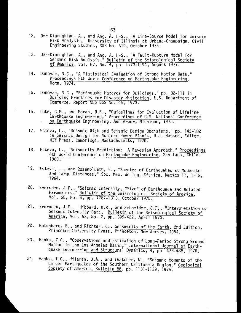
6312. Der-Kiureghian, A., and Ang, A. H-S., IIA Line-Source Model for Seismic
Risk Analysis,1I University of Illinois at Urbana-Champaign, CivilEngineering Studies, SRS No. 419, October 1975.
13. Der-Kiureghian, A., and Ang, A. H-S., "A Fault-Rupture Model forSeismic Risk Analysis,1I Bulletin of the Seismological Societyof America, Vol. 67, No.4, pp. 1173-1194, August 1977.
14. Donovan, N.C., IIA Statistical Evaluation of Strong Motion Data,"Proceedings 5th World Conference on Earthquake Engineering,Rome, 1974.
15. Donovan, N.C., "Earthquake Hazards for Buildings," pp. 82-111 inBuilding Practices for Disaster Mitigation, U.S. Department ofCommerce, Report NBS BSS No. 46, 1973.
16. Duke, C.M., and Moran, D.F., "Guidelines for Evaluation of LifelineEarthquake Engineering," Proceedings of U.S. National Conferenceon Earthquake Engineering, Ann Arbor, Michigan, 1975.
17. Esteva, L., IISeismic Risk and Seismic Design Decisions," pp. 142-182in Seismic Design for Nuclear Power Plants, R.J. Hansen, Editor,MIT Press, Cambridge, Massachusetts, 1970.
18. Esteva, L., "Seismicity Prediction: A Bayesian Approach,1I Proceedings4th World Conference on Earthquake Engineering, Santiago, Chile,1969.
19. Esteva, L., and Rosenblueth, E., "Spectra of Earthquakes at Moderateand Large Distances," Soc. Mex. de Ing. Sismica, Mexico 11, 1-18,1964.
20. Evernden, J.F., "Seismic Intensity, "Size" of Earthquake and RelatedParameters'" Bulletin of the Seismological Society of America,Vol. 65, No.5, pp. 1287-1313, October 1975.
21. Evernden, J.F., Hibbard, R.R., and Schneider, J.F., "Interpretation ofSeismic Intensity Data,1I Bulletin of the Seismological Society ofAmerica, Vol. 63, No.2, pp. 399-422, April 1973.
22. Gutenberg, B., and Richter, C., Seismicity of the Earth, 2nd Edition,Princeton University Press, Princeton, New Jersey, 1954.
23. Hanks, T.C., "0bservations and Estimation of Long-Period Strong GroundMotion in the Los Angeles Basin," International Journal of Earthquake Engineering and Structural Dynamics, 4, pp. 473-488, 1976.
24. Hanks, LC., Hileman, J.A., and Thatcher, W., "Seismic Moments of theLarger Earthquakes of the Southern California Region,1I GeologicalSociety of America, Bulletin 86, pp. 1131-1139, 1975.

--------
64
25. Housner, G.W., "Measures of Severity of Earthquake Ground Shaking,"Proceedings of U.S. National Conference on Earthquake Engineering,Ann Arbor, Michigan, 1975.
26. Iida, K., "Earthquake Energy and Earthquake Fault," Nagoya University,Journal of Earth Science, Vol. 7, No.2, pp. 98-107, 1959.
27. Johnson, J.J., and Robinson, A.R., "Wave Propagation in a Half Spacedue to an Interior Point Load Parallel to the Surface," Universityof Illinois at Urbana-Champaign, Civil Engineering Studies, SRS,No. 388, July 1972.
28. Japan Road Association, "Research on Earthquake Protection of PetroleumPipelines," Tokyo, Japan.
29. Kagan, Y., and Knopoff, L., "Earthquake Ri sk Predi cti on as a Stochasti cProcess," fbisics of the Earth and Planetory Interiors, 14 (1977),pp. 97-108.
30. Kanai, K., "An Empirical Formula for the Spectrum of Strong EarthquakeMoti ons," Bulleti n, Earthquake Research Institute, 39, pp. 85-95,1961.
31. Kanai, K., "Improved Empirical Formula for the Characteristics ofStrong Earthquake Motions," Proceedings Japan Earthquake EngineeringSymposium, Tokyo, Japan, pp. 1-4, October 1966.
32. King, Y., and Knopoff, L., "Stress Drop in Earthquakes," Bulletin ofSeismological Society of America, Vol. 58, No.1, pp. 249-257,February 1968.
33. Lin, Y.K., Probabilistic Theory of Structural Dynamics, R.E. KriegerPublishing Co., Huntington, New York, 1976.
34. McGuire, R.K., "Seismic Structural Response Risk Analysis, IncorporatingPeak Response Regressions on Earthquake Magnitude and Distance,"MIT Department of Civil Engineering, Research Report R74-51, 1974.
35. Milne, W.G., "Measures of Severity of the Earthquake Ground Shaking,"Proceedings of U.S. National Conference on Earthquake Engineering,Ann Arbor, Michigan, 1975.
36. Newmark, N.M., "Comments on Conservatism in Earthquake Resistant Design,"Report to U.S. Nuclear Regulatory Commission, September 1974.
37. Newmark, N.M., Hall, W.J., and Mohraz, B., "A Study of Vertical andHorizontal Earthquake Spectra," Directorate of Licensing U.S. AtomicEnergy Commission, Report WASH-1255, April 1973.
38. Newmark, N.M., and Hall, W.J., "Pipeline Design to Resist Large FaultDisplacement," Proceedings U.S. National Conference on EarthquakeEngineering, Ann Arbor, Michigan, 1975.
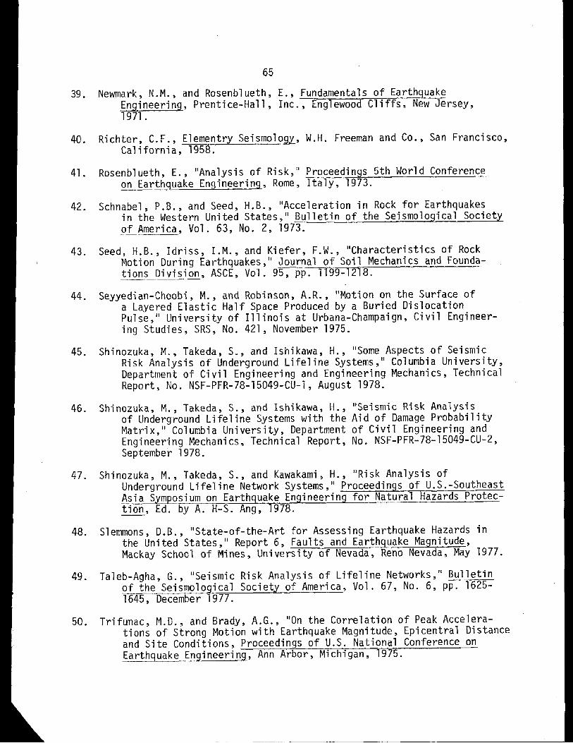
-- -- - ~- --~--~~-
65
39. Newmark, N.M., and Rosenblueth, E., Fundamentals of EarthquakeEngineering, Prentice-Hall, Inc., Englewood Cliffs, New Jersey,1971.
40. Richter, C.F., Elementry Seismology, W.H. Freeman and Co., San Francisco,California, 1958.
41. Rosenblueth, E., IIAnalysis of Risk," Proceedings 5th World Conferenceon Earthquake Engineering, Rome, Italy, 1973.
42. Schnabel, P.B., and Seed, H.B., "Acceleration in Rock for Earthquakesin the Western United States,1I Bulletin of the Seismological Societyof America, Vol. 63, No.2, 1973.
43. Seed, H.B., Idriss, I.M., and Kiefer, F.W., "Characteristics of RockMotion During Earthquakes,1I Journal of Soil Mechanics and Foundations Division, ASCE, Vol. 95, pp. 1199-1218.
44. Seyyedian-Choobi, M., and Robinson, A.R., IIMotion on the Surface ofa Layered Elastic Half Space Produced by a Buried DislocationPulse,.1 University of Illinois at Urbana-Champaign, Civil Engineering Studies, SRS, No. 421, November 1975.
45. Shinozuka, M., Takeda, S., and Ishikawa, H., lI$ome Aspects of SeismicRisk Analysis of Underground Lifeline Systems,1I Columbia University,Department of Civil Engineering and Engineering Mechanics, TechnicalReport, No. NSF-PFR-78-15049-CU-l, August 1978.
46. Shinozuka, M., Takeda, S., and Ishikawa, H., IISeismic Risk Analysisof Underground Lifeline Systems with the Aid of Damage ProbabilityMatrix,1I Columbia University, Department of Civil Engineering andEngineering Mechanics, Technical Report, No. NSF-PFR-78-15049-CU-2,September 1978.
47. Shinozuka, M., Takeda, S., and Kawakami, H., IIRisk Analysis ofUnderground Lifeline Network Systems,1I Proceedings of U.S.-SoutheastAsia Symposium on Earthquake Engineering for Natural Hazards Protection, Ed. by A. H-S. Ang, 1978.
48. Slemmons, D.B., IIState-of-the-Art for Assessing Earthquake Hazards inthe United States, II Report 6, Faults and Earthquake Magnitude,Mackay School of Mines, University of Nevada, Reno Nevada, May 1977.
49. Ta1eb-Agha, G., IISeismic Risk Analysis of Lifeline Networks,1I Bulletinof the Seismological Society of America, Vol. 67, No.6, pp. 16251645, December 1977.
50. Trifunac, ~1.D., and Brady, A.G., liOn the Correlation of Peak Accelerations of Strong Motion with Earthquake Magnitude, Epicentral Distanceand Site Conditions, Proceedings of U.S. National Conference onEarthquake Engineering, Ann Arbor, Michigan, 1975.

-----
66
51. Weidlinger, P., and Nelson, 1., "Seismic Analysis of Pipeline withInterference Response Spectra," Weidlinger Associates, ConsultingEngineers, Grant Report, No.7, June 1978.
52. Whitman, R.V., Cornell, C.A., and Taleb-Agha, G., "Analysis of Earthquake Risk for Lifeline Systems," Proceeding~_of the U.S. Nationa_lCo_n!eren~~~_ Eart~.9-~Js~_Engi!l~~ri!1.9, Ann Arbor, Mi chi gan, 1975.

TABLE 2.2 SUMMARY OF VERTICAL TO HORIZONTALvIa RATIOS (REF. 37)
* Actually alluvium values only since all rock components had peak groundaccelerations> O.lg (horizontal) and 0.059 (vertical) (Ref. 37).
* Actually ·a1luvium values only since all rock components had peak groundaccelerations> O.lg (horfzontal) and 0.059 (vertical) (Ref. 37).
No. of Average vIa - verticalrecords vIa - horizontal
28 0.92
22 0.92
6 0.91
15 0.85
9 0.81
*13 0.99
No. of Average a - verticalrecords a - horizontal
28 0.53
22 0.53
6 0.54
15 0.65
9 0.72
*13 0.40
a11 uvi urn & rockah > O.lg, av > 0.05g
alluvium,ah > O.lg, av > 0.05g
alluvium &rock,ah < O.lg, av < 0.05g
rock
alluvium
67TABLE 2.1 SUMMARY OF VERTICAL TO HORIZONTAL
ACCELERATION RATIOS (REF. 37)
Site
a11 uvium & rock
Site
all uvi urn
all uvi urn & rock
rock
alluvium & rock,ah > O.lg, av > 0. 05 9
alluvium alone,ah > O. 19, av > O. 05g I
alluvium &rock,ah <0.19, av <0.05g

------- - ~--~~~~--~~~~~~~~~~~~-
68
TABLE 2.3 SUMMARY OF AVERAGE ad/v2 VALUES (REF. 37)
No. of 2Site Direction Records ad/v
alluvium & rock horizontal 28 5.6all uviLm horizonta1 22 5.7rock horizontal 6 5.4
alluvium & rock, horizontal 20 5.7a > o. 19
alluvium, horizonta1 14 5.9a > o. 19
rock, a > 0.1 9 hori lontal 6 5.4(same as above)
alluvium, horizontal 8 5.3a < O.lg
all uvi urn & rock* vertical 14 10.7alluvium &rock vertical 13 9. 1all uvi um* verti ca1 11 10.0all uvi urn vertical 10 7.9rock vertical 3 13.0
all uvi urn & rock, vertical 8 12.4f1 > 0.05g
all uvi urn, vert i ca1 5 12.0a > 0.05g
all uvi urn, vertical 4 7.3*a > 0.05g
rock, a > 0.05g verti ca1 3 13.0(same as above)
alluvi urn, vertical 6 8.4a < 0.05g
* Not including the one extreme value, El Centro, 5-18-40, 2037 PST,vertical component ad/v2 = 30.58 (Ref. 37)
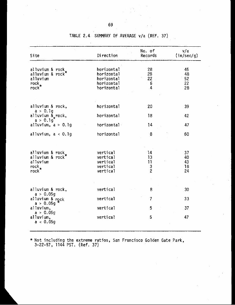
~- -~-_._---~--------
* Not including the extreme ratios, San Francisco Golden Gate Park,3-22-57, 1144 PST. (Ref. 37)
3740431824
14131132
No. of viaDirection Records (in/sec/g)
horizontal 28 45horizontal 28 48horizontal 22 52horizontal 6 22horizontal 4 28
verticalverticalverti ca1verticalvertical
TABLE 2.4 SUMMARY OF AVERAGE via (REF. 37)
69
alluvium & rock, vertical 8 30a > 0.05g
alluvi urn &r~ck vertical 7 33a > 0.05g
all uvi urn, verti cal 5 37a > 0.05g
alluvium, verti cal 5 47a < 0.059
alluvium & rock, horizontal 20 39a > O.lg
all uvi urn &*rock, horizontal 18 42a>O.lg
alluvium, a > 0.19 horizontal 14 47
all uvi urn, a < 0.19 horizontal 8 60
alluvium & rockalluvium & rock*alluviumrock*rock
all uvi urn & rockalluvium & rock*all uvi urnrock*rock
Site
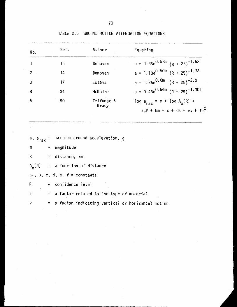
70
TABLE 2.5 GROUND MOTION ATTENUATION EQUATIONS
No. Ref. Author Equation
15 Donovan a = 1.35eO. 58m (R + 25)-1.52
2 14 Donovan a = 1.10eO. 50m (R + 25)-1.32
3 17 Esteva a = 1. 26eO. 8m (R + 25) -2.°4 34 McGui re a = O.48eO.64m (R + 25)-1.301
5 50 Trifunac & log a = m+ log Ao(R) +Brady max
a,P + bm + c + ds + ev + fm2
a, amax = maximum ground acceleration, g
m = magnitude
R = distance, km.
Ao(R) = a function of distance
a1' b, c, d, e, f = constants
P = confidence level
s = a factor related to the type of material
v = a factor indicating vertical or horizontal motion

71
TABLE 4.1 VALUES OF e FOR TYPE 3 SOURCE
Case Governing Inequality 8
1 o > s/2 O.
2 011 > 0 1 > s/2-1 21yl
2cos --s
-1 21yl x3 D" > s/2 > 0 I cos --+ tan- l -
s Iyl
-1 2. - xtan- l xx
4 s/2 > 011 > 0 1 tan J +Iyl Iyl
In table 5.1, x and yare coordinates of ~A; and 2j is the length of
1ink j; and,
01 = distance from ~A; to the nearest end of the link;
~I = distance from ~A; to the farthest end of the link.

TABL
E6.
1AN
NUAL
PRO
BABI
LITY
OFFA
ILU
REIN
APA
TH(T
OK
YO
)
Mea
nL
ink
Res
ist.
ing
's
Pat
h·1
50.2
25.3
00
.375
.45
0.5
25.6
00
1.1
603
.79
x10
-21.
17x
10-2
3.9
3x
10-3
1.4
x10
-35.
15x
10-4
1.95
x10
-4
2.1
603
.79
x10
-21.
17x
10-2
3.9
3x
10-3
1.4
x10
-35.
15x
10-4
1.95
x10
-4
3.1
30-2
9.3
2x
10-3
3.1
4x
10-3
1.1
2x
10-3
4.12
x10
-41.
56x
10-4
3.0
4x
10
4·1
303
.04
x10
-29
.32
x10
-33
.14
x10
-31.
12x
10-3
4.12
x10
-41.
56x
10
5.2
957.
43x
10-2
2.3
3x
10-2
7.8
6x
10-3
2.81
x10
-31.
03x
10-3
3.8
9x
10-4
6.2
455
.99
x10
-21.
86x
10-2
6.29
x10
-32
.25
x10
-38
.24
x10
-43.
11x
10-4
-...J
N
7.2
455
.99
x10
-21.
86x
10-2
6.29
x10
-32
.25
x10
-38
.24
x10
-43.
11x
10-4
8·1
603
.79
x10
-21
.17
x10
-23
.93
x10
-31
.4x
10-3
5.15
x10
-41.
95x
10-4
9.2
205.
26x
10-2
1.63
x10
-25
.5x
10-3
1.97
x10
-37.
21x
10-4
2.7
2x
10-4
10.2
205.
26x
10-2
1.63
x10
-25
.5x
10-3
1.9
7x
10-3
7.21
x10
-42
.7x
x10
-4
11·1
603
.79
x10
-2-2
3.9
3x
10-3
1.40
x10
-35
.15
x10
-41.
95x
10-4
1.17
x10
12.0
992
.29
x10
-26.
99x
10-3
2.3
6x
10-3
8.4
3x
10-4
3.0
9x
10-4
-41.
17x
10
13.1
89-2
1.40
x10
-24.
72x
10-3
1.6
9x
10-3
-42
.33
x10
-44.
53x
106
.18
x10
14·1
303
.04
x10
-29.
32x
10-3
3.1
4x
10-3
1.1
2x
10-3
-41.
56x
10-4
4.12
x10

TABL
E6.
2AN
NUAL
PROB
ABIL
ITY
OFFA
ILUR
EOF
SUPP
LYNE
TWOR
K(T
OKYO
)
Mea
nLi
nkR
esis
t.in
g's
.150
.225
.300
.375
.450
.525
.600
A+9
3.33
x10
-3-5
1.28
x10
-64.
85x
10-8
4.37
x10
B~9
1.21
x10
-3-6
3.72
x10
-84.
05x
10
C~9
.130
-29.
32x
10-3
3.1
4x
10
-31.
12x
10-3
-4-4
3.04
x10
4.12
x10
1.56
x10
...... w

74
TABLE 6.3 IDEALIZATION OF SOURCES FOR BOSTON AREA
Number Type Occurrence Mu MoRate
1 3 0.024 6. 1 4.3
2 3 0.008 6.8 4.3
3 3 0.004 5.5 4.3
4 3 0.028 5.9 4.3
5 3 0.020 5.2 3.7
6 3 0.0125 5.5 4.3
7 3 0.032 5.5 4.3
8 3 0.0375 5.9 4.3

75
TABLE 6.4 ANNUAL FAILURE PROBABILITY OF LINK
Fault-Rupture Ground Shaking,Link Strike Yr ;:: 0. 0769
1 0.000012 0.000678
2 0.000015 0.001226
3 0.000024 0.000660
4 0.000013 0.001226
5 0.000086 0.001572
6 0.000083 0.004469
7 0.000094 0.004469
8 0.000055 0.000465
9 0.000123 0.001252
10 0.000185 0.001957
11 0.000096 0.001957
12 0.000084 0.001961
13 0.000117 0.000315
14 0.000029 0.000531
15 0.000077 0.000994
16 0.000069 0.000995
17 0.000043 0.002226
18 0.000043 0.000678
19 0.000118 0.000680
20 0.000017 0.004469
21 0.000029 0.000405
22 0.000087 0.000405

76
TABLE 6.5 EQUIVALENT PARALLEL PATHS FOR BOSTON HIGHWAYS"-
No. of Annual Fail. Prob.Path Links Links Rupture Ground
Str; ke Shaking
1 12 15-21-13-l1-10-9-8-7-20-18-2-5 0.00103 0.02094
2 12 15-21-13-10-9-16-17-19-18-20-6 0.00091 0.02024
3 10 15-22-14-9-8-7~20-18-2-5 0.00068 0.01598
4 . 9 15-21-13-11-10-9-5-7-6 0.00065 0.01581
5 10 15-22-14-9-16-17-19-18-20-6 0.00065 0.01538
6 9 3-4-2-19-17-16-8-7-6 0.00045 0.01519
7 6 3-4-2-18-20-6 0.00021 0.01428
8 7 1-19-17-1 6- 8- 7- 6 0.00021 0.01275
9 11 15-21-13-11-10-9-16-17-19-2-5 0.00086 0.01187
10 4 1-18-20-6 0.00016 0.01185
11 7 15-22-14-9-8-7-6 0.00055 0.01095
12 9 15-22-14-9-16-17-19-2-5 0.00065 0.00701
.13 3 1-2-5 0.00011 0.00490
14 3 3-4-5 0.00012 0.00350

o
oQ
II)
0 0~ .......c u..C' w0 0:::
~C\I
Q0
ro - 0:::en
~u..
d o::r:+ I-
o::r:<D E
0..........
10 -'If: <;;t
<D
~AIII
E ::E
0:::C 0u..
'0 ~r-
0
V)
=:JV)0:::l.J..J::::-W0:::JI-.......Zc.!J
N ;E• '0
N.c.!J• .......l.J...
77
•
•
•
'- ~ _J. I_ ~----..L----..... 't'loro

FIG. 2.2 TWO-DIMENSIONAL FAULT MODEL (DIP-SLIP)
z
o
Fault Plane
Fault Plane
x
x
,e::..---""'~f------Y
78
h
Free Surface
h
FIG. 2.3 TWO-DIMENSIONAL FAULT-MODEL (STRIKE-SLIP)
Free Surface

y
x
... ..".Iult. in the far- r.gionare not r.'.... becauseof 2-D a",roximotion
W=2
IO-J....__...._ ......._L-......."""-I.-'-....... ......_ .....__...... ~
I 10
Epicentrol DiltOftCe D. km
FIG. 2.4 VARIATION OF az/Dz WITH D FOR DIFFERENT W(h = 15 km, Y = 900 )
1.0,....--~-~....,.-.,-.,...,..."T""'I".,....--..,..--r---,r-~...,."T"T,
79
- 10
24,20km
E.......at
.5N
o.......
No
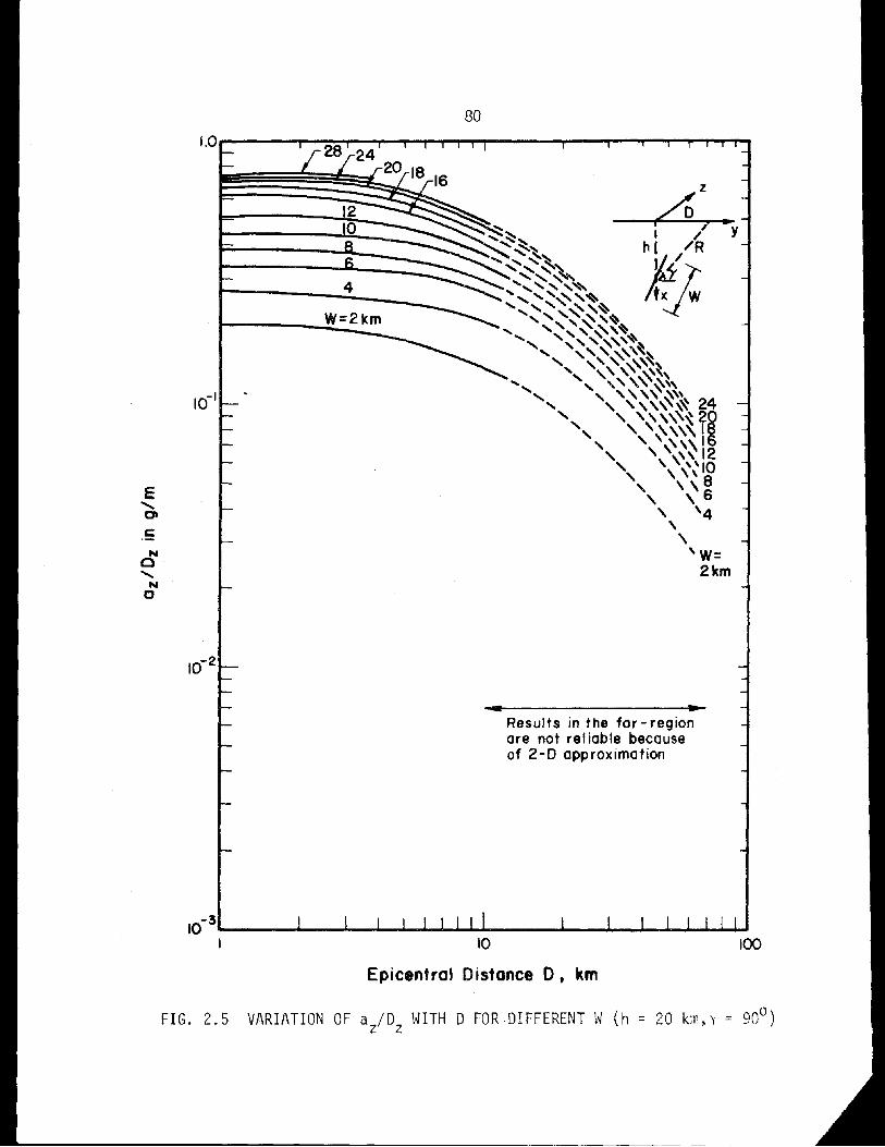
z
A
Results in the for-regionore not reliable becauseof 2-D approximation
80
W=2km
- -~ -- ----------------------------
1.0_----,.-=-r--..,...~....,......._.,...,._,_---..._-.,..__,.__r~_,......_,...
IO-3....__-.l....._""--.-...--'I...-I~_I_~ _I__.....,I,_~~~...t_...I...I.~
I ~ 00
Epicentral Distance D t km
FIG. 2.5 VARIATION OF az/Dz WITH D FOR·DIFFERENT W(h = 20 km,Y = 900)
E"Cl
.scS"...o

20
killR =15
81
8 10 12 14 16 18 20 22 24
W, km
246
FIG. 2.6 VARIATION OF a /D WITH WFOR h = 15 AND y = 90°z z
I.0 r----,r---"T--r"-..,..-,.....--r-~-~-----...----
0.010
E30
.......01
c: 40
N 0.1c 50.......
N 600
70
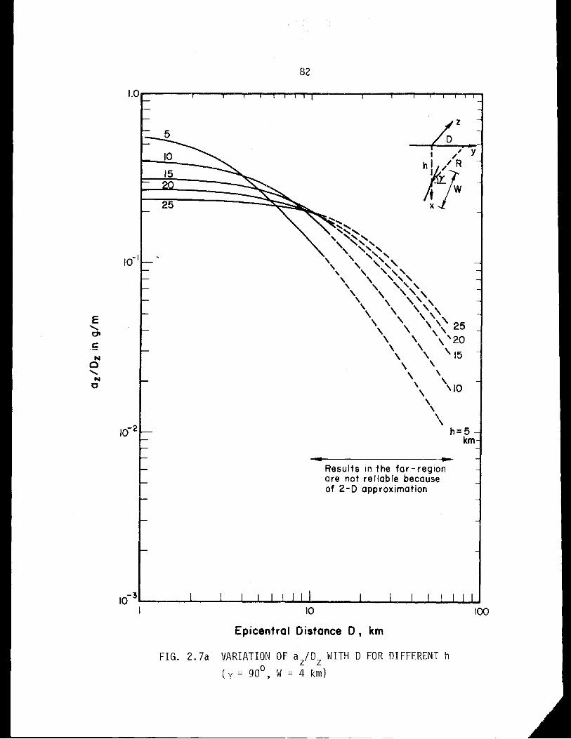
100
I / Y
~}:"00.,~~,, ,,~,, '", ""\. '\ '~,~," , ",, , ,,'" , ',','" " ,,', ' ",,", , ",
, " " ,,, 25, \ "\ , , '20\ \
\ , '15\ \, \
\\ \10
\\
\
\h=5
km
Results in the far- regionare not reliable becauseof 2-D approximation
... -
82
--------------------------
10
Epicentral Distance 0 1 km
15
10
25
FIG. 2.7a VARIATION OF az/Dz WITH 0 FOR DIFFERENT h(y = 90°, W = 4 km)
1.0 r------r-~r__...,.......,......,......,....,...,....,...--.......,r__-,...___.____r'....,.....,.. ........._.
10-3 .......__......--'-........................."""'-J. ......._--l._...l-....L-....L-...L..~
I
E......Cl
.£N
o......
NC

~~':'-",~"~, '"",, ""," '" ,~~~," ,',,~,, ' ",'" " ',,~,, ' "',, ", , ,'~25
, , , 20',\ , 15, ', \
, '10,,'h=5km
R.,ult, in the 1ar- r'Qionare not rill." becauseof 2-0 approximation
83
/~, •• y, /~
1 /.
~- ..
FIG. 2.7b VARIATION OF a /0 WITH 0 FOR DIFFERENT ho z z
( y = 90 , W= 10 km)
to-S'-__......._'""'-........L..........~.J-_-~_...I---J_w..J....L.J.J
I 10 100
Epicentral Distance D t km
1.0.....---r--r-..,......,....,..,-,-,...,..--...,.-...,.........,......,-.......,.---
e......'".f:N
o......
No
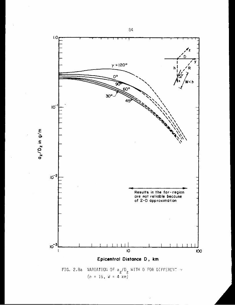
1.0,..-----r--,.....--r--r--r--r-r-T"'I"'----r--.....,..-...,..--r--r-...,...,...,....
tlz"/
" 0, ,.I / 'I
/
h~(R
jt~<h
Results in the for - regionore not re Iiab Ie becauseof 2-D approximation
~-- ------------~----- ----------- ---- ~--------------
.... ....
84
y =1200
VARIATIOn OF a /0 WITH 0 FOR DI FFEREIH "(z z(h = 15, W= 4 km)
FIG. 2. 8a
10-3~____I._ ___I_-'-......L........L.._'_.I_I.~_____JI._..__"'____l..__l.__J.....L...J_U
I ~ 00
Epicentral Distance D t km
E"01
c::...
o"...o

Results in the 1ar- regionare not reliable becauseof 2-D approximation
85
IO-3"-__......._ ......._'--"'--~-6-,&"",I,., '--_oI...............................
I ~ 100
Epic."trol Oistonce 0, km
FIG. 2.8b VARIATION OF az/Dz WITH D FOR DIFFERENT y
(h = 15, W= 20 km)
e........Ot
.5
tS...........o

100
Results In the far - regionare not re I iab Ie becauseof 2-D appro)(Imation
- ...
116
10
Epicentral Distance D 1 km
-- -~---~_.~- --~ -------------------
E,01
C
)(
o,>.
o
FIG. 2.9 VARIATIOil OF a /0 ~/ITH D FOP. DIFFEREnT viy x
(h = 15, O( = 90°, vp/vs = 1.75)

.... ..Re.ulfs in the far-reQionare not reliable becauseof 2-0 approximation
87
FIG. 2. 10 VARIATION OF ay/Dx WITH D FOR DIFFERENT W(h = 20 km, y = 90°, vp/vS = 1.75)
IO-3~__......._....,I,_""-""''''''''''''''-'''"",,,-''--__-'-_'''''_'''--''''-''''''I...oI.'''''''I ~ 00
Epicentrol Oistonce 0, km
e......at
.5)(
o......
>o

y
z
Results in the far- regionare not reliable becauseof 2-D approximation
,,\, ,, ,
\ \\ \,\ \ \'-o\--\- ...
\ \ "\ \ ,\ \ \\ \ " ....,, \ ,
''-\ 1'\-~ / "\'...... \~h=IOk
\ "" 15\ I,\ I ,
\, ' ... 20\ J...
... ...
88
-- --~- ~---~-------------------------
10-3L-__.....L_---i~....L-....L.....I-...J...J_I..J___._L__.L._.....J.___L........l......J...J_u
I 10 100
Epicentral Distance D, km
FIG. 2.11 VARIATION OF ay/Dx WITH D FOR DIFFERENT h(W = 4 km, y = 900, Vp/vs = 1.75)
E.......0'
.s)(
o.......
>o
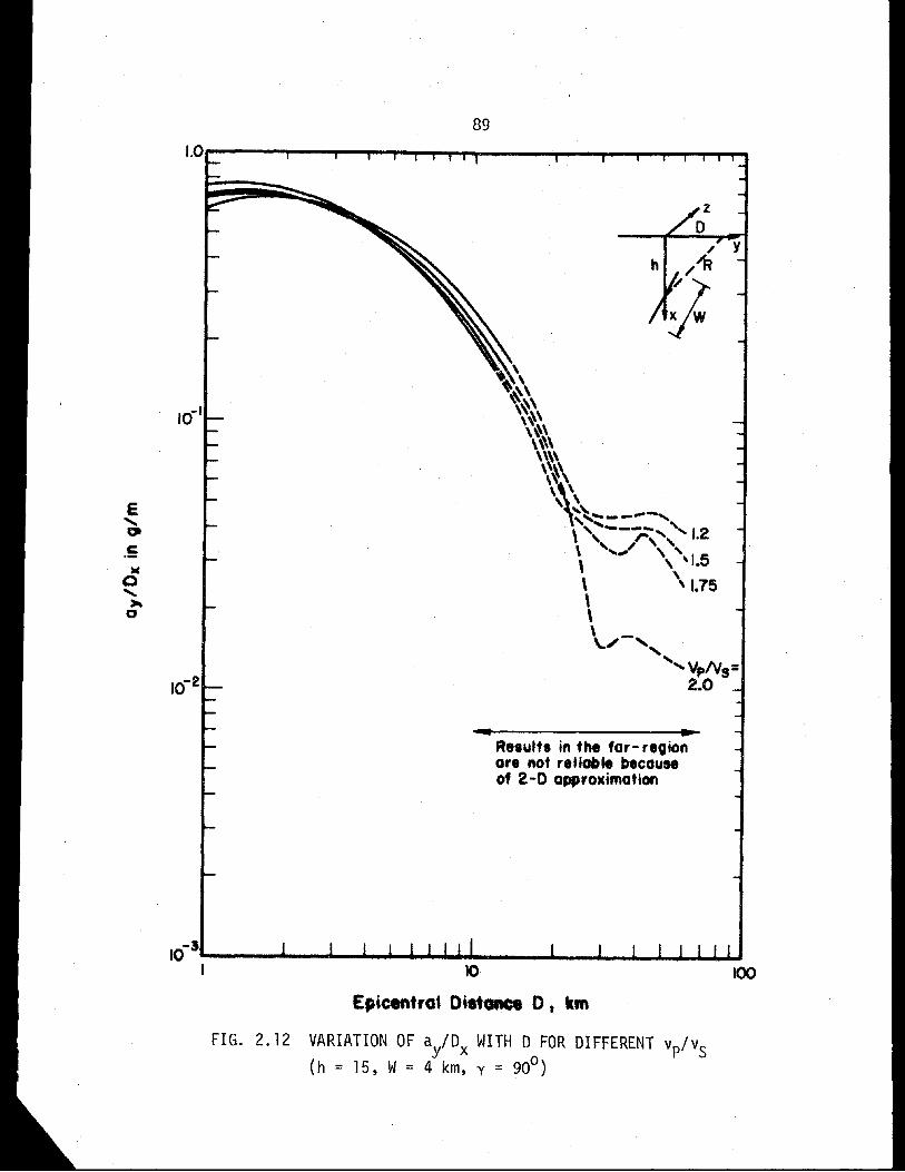
.... ...Retultt in the for- regionare not reUable becauseof 2 -0 approximation
89
IO-3"-__....._ ..._~......'-"__........ ~_................................,I to 100
E,icentral DistClNe 0 t km
FIG. 2.12 VARIATION OF ay/Dx WITH D FOR DIFFERENT vp/vs(h = 15, W= 4 km, y = 90°)
e......at
.5M
Q......>lo
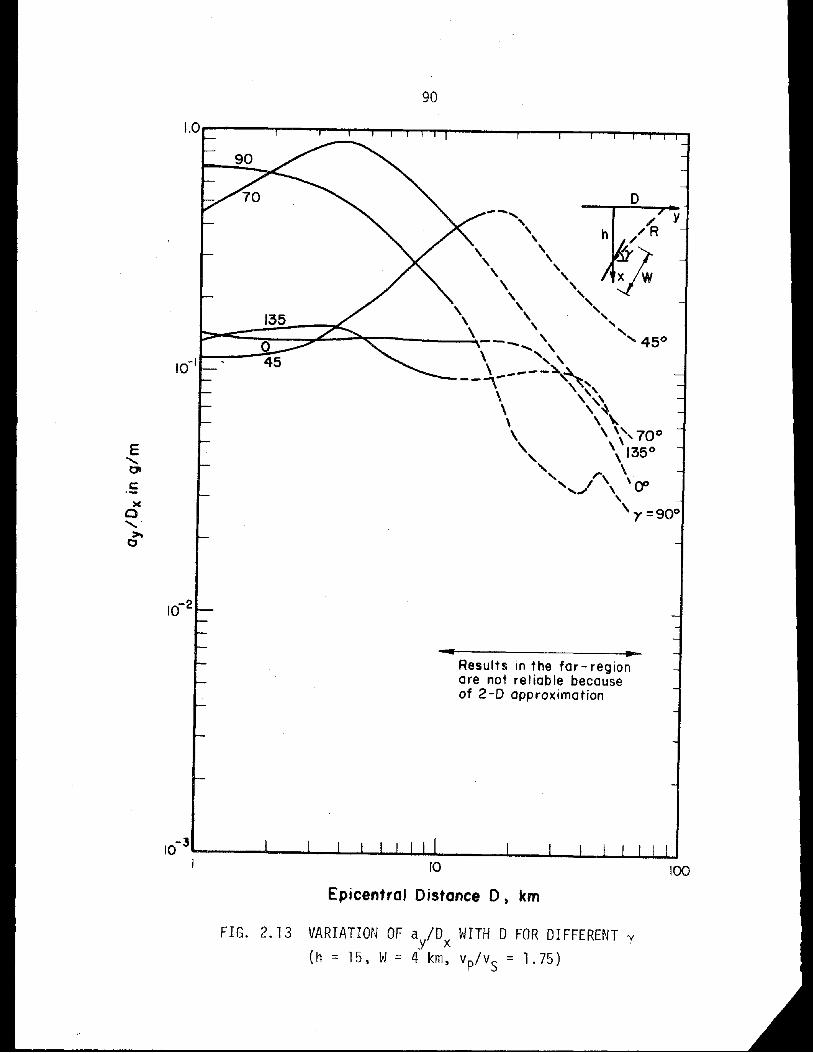
yD
h--....,
\\
\\
\\.
\.
'""", , 450
,,,\ ,,,
~c:::::::;==:::::~~~ ~\.__ \,F _ ..... ,
\ '"\ ---~~-- ...---, '" "
\ \. \.'
\. "\ , ~
\ \ \.\ \ \~, 10°
" \ 1350
, r \" I \ \ rD...."'" , v-,
'y =900
FIG. 2.13 VARIATION OF ay/Dx
WITH 0 FOR DIFFERENT y
(h = 15, W= 4 km, vp/vS = 1.75)
Results in the far- regionare not re Iiab Ie becauseof 2-D approximation
90
- ...
10-3'----....&.-.....'--....l-....l-....l-...J-..L..J...J- l..-_J.--J..--L-J.-J....L.U
I 10 100
EpicentraJ Distance D J km
E......Ol
c:)(
o......>o

)(
.",.----- .......---- "::---" '\---- " \, ",,-,:-," \"" ,''\ \, '\" '\--- \~\. \'",'" ',\ \\ \ '\
'\ \ ~ \ '18, \"~ \\ \ ~~ 14\ \ ~\ ,+10\ "8
\ \ 6\\ W =4km
o
Results in the for-regionor' not reflable becauseof 2 -0 approximation
- ..
91
1.0r----r--..,..-----r--r...,...,..T"?'-r-----...,..---.~,........-.......-
10-3.....__..._ ....--a.....,/,.........L....L.J"...l.-__..L._..J.......J~L...J...J...u.J
I ~ 00
Epic.trat Distance D I km
FIG. 2.14 VARIATION OF a /0 WITH D FOR DIFFERENT Wx xo(h = 15 km, y = 90 , vp/vS = 1.75)
e......o.5•c......•o
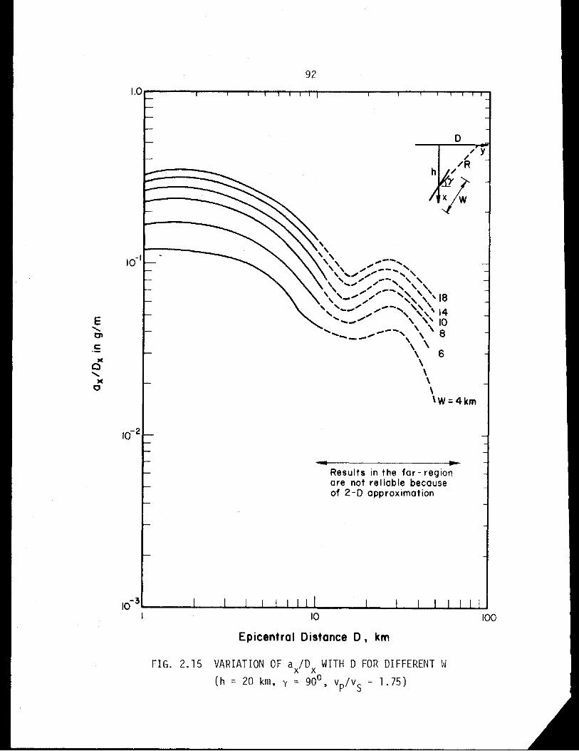
yo
Results in the far- regionare not reliable becauseof 2-D approximation
... ...
,,",, , "',,--...." '" -- ', ,.... ",'" , ", ' -, " ", " "'" '" ....--,,,,,,,, -'" ........ '" , ' 18" '--'" ",--, ,,, \ 14, .... " ",........_..... , " 10
..... ---, ' \ 8...._--- \ \\ \\ 6\\\\\W =4km
92
VARIATION OF a /0 WITH 0 FOR DIFFERENT Wx x(h = 20 km, y = 90°, vp/vS = 1.75)
FIG. 2.15
1.0,.---....,.----,r---r---r-,-..,.....,....,...,----r---or--"-""T".......,.--r"-""T"..,....,....,
10-3~----.l._--'_...l---'---'-...l-.L...I.....L- __......II.-_J.-....J...--l......L....J...-UU
I 10 100
Epicentral Distance D, km
E"'0'c:)(
o"'
)(
o
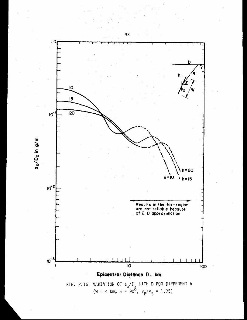
E.......01
.sMo
.......M
o
931.0,.....--...,....--r-....,..-.,..-r.,...,....,..,r----..,....-or--~ ......._
y
20
-...." \
;,,"~';" \ ",; ,,;Jr~,..._... \ \ \
\ \ \\ '\\ \ \\ \ \\ \ \\ \ \ h=20
\ \
h =10 'h=15
.. ..Results in the 1ar- regionare not reliable becauseof 2-DapproICimation
to-I~-_"'-_L...-.J-...L.-w....L..J.J....--...l--..l.-..L...L....Lu.lJI ~ 00
Epic.trol Dittonce 0, km
FIG. 2.16 VARIATION OF ax/Ox WITH 0 FOR DIFFERENT h(W = 4 km, y = 900
, vp/vs = 1.75)

100
Results in the 10r- regionare not re Iiab Ie becauseof 2-D approximation
...-....~--,',
..........., "~.".....- .....~, "
\' \\,\ \,\\ \,\\ '\\\ \\\\ \\\\ \\\~\ \~ 1.5
" \1.75\ 1.2\
Vp/VS =2.0
- ...
94
0
/ Y
1.2
h~1.5 x W
10
Epicentral Distance D, km
FIG. 2.17 VARIATION OF ax/Ox WITH 0 FOR DIFFERENT vp/vS(W = 4, h = 15 km, y = 90°)
)(
c........
)(
o

95
o
..Resultl in the for- regionore not r.Haole becauseof 2-D approximation
...
FIG. 2.18 VARIATION OFax/Dx WITH D FOR DIFFERENT y(W = 4, h = 15 km, vp/vS = 1.75)
1.0----w--...,..-.....,..-,...,....,..,...,..---.....- .....-r--r-..,.....,..,r-r-1
1O-3L..__......_....L.-......Io--"--"-'-...........__....._ ..........,j...........................I ~
Epicentral Oi,tClftCe 0, km
E
"01
.E)C
o")C
o

Donovan
96
Esteva
---- Eq. 2.23 (W=5. y =90. h=20)_.- Eq. 2.27 (y= 90. h =20)
FIG. 2.19 ATTENUATION OF MAXIMUM GROUND ACCELERATION(m = 7.0)
------'-'--."""-.",----- ~-- "'t:=------------.-,;:-::::.-..,-=:--___ -"'-...._:::::"
10-2.....----I.-.......L._.................L...J.....&....I~__....L.._ __L._"'__..I_.J.......J~...L.J
f ~ 00
Epicentral Distance D. km
1.0
0-
s:.2-0~
Q)
G>00<t'"0s:::30~
(!)
~0:E 10-1

-EnteringPoint
97
Final Point
N1........---....-...;;...----~ ..........Entering Final
Point Point
FIG. 4.1 SIMPLE LIFELINE NETWORKS

8Fault
Link j
b
___D=..2_J. J
FIG. 4.4 TYPE 3 SOURCE
98
a
Fault 8
FIG. 4.2 TYPE 1 SOURCE
a
y
b
A
FIG. 4.3 TYPE 2 SOURCE

.c
.&ot-
o.-~
Q)>0/\C0>-0Q)Q..Q)o)(
W
o;:,cc«
99
Yr
Ground Motion Intensity, y
FIG. 5.1 ANNUAL PROBABILITY OF EXCEEDANCE
Yr
FIG. 5.2 PDF OF LINK RESISTANCE
Yr

Final
Point
100
1)-----.0- - - --O- +-...JJ
FIG. 5.3 A NETWORK OF PARALLEL PATHS
P-----"C- - - - - -0----"0
~----o()--- --.- - 0-_---0..
,---_ ...... _.-_--
-- -------_ ... _------- -- -----~~. -_.~-----------
Point
Entery

101
D Wat.r Supply Station... Direction of Flowo Node of Pipeline
5 kmo
FIG. 6.1 WATER SUPPLY NETWORK FOR TOKYO
CD -e=:_13 -

t.
••
'"• ° .i-6/' /."....
• •••j,-
102
•• •
~--.
+
Ii.: 4
• & .~ • • ,1..........A~ AJa,
••• ••••• A. <DO••••
•• • ~Jj .0OC'• -I" _: I. •• +••• '! • .i.: ~... 60! , ~.~~
• •• 660
•• ~ ? ... 6 (.",fa$, 1>~1.:~ 6
0 !. .':'~ ••" 6 ~ • \t'00·.,61 • , I , ••••
• • • 0 CI.. .. lO. 0 I e4 •I ._!l.~A'" f~~.ll.-J....... !'. q, , ...;. • 0 4ia~'" ~ ··JII~~·O '-: 1-•• : • •I" .lio... &1>0.~. 'QI?-. ct.- .,;:,. "'1 c.••I : ~ ot- ~ I cfl'1~'•• - • 'l.'. ~.'
• 0 .. L> ~ .• ~~cY ,... • ..'t •• ,•,'" ..6 O~: o~~~i. • ....0". "" oj •••••6 ,0.. ,.,_it •• ~ .._~ •No ... 0,; • • /~ • • 0
.+ • :';JL:. "'~6+.~}.~;'" · o~,;:i+ ..'6·: '1·. ::-.... 8.;'.... .... P. •••• ::rl~•. 0.· .~I..Q)•• '. • ~O!i' .01..0· .
0' t":'.. 0 f46660_~'O.. ..••• j.. •• I .0. ~. •• • •• 'Il ~ • o. ~:. o.~ .
• .,., n ...• ° 6'D •..... \°0 •
•••"'.. • •• A~. ... .,..
6.2 EPICENTER ~~P OF TOKYO BAY AREA(1961-1970) -- FROM REF. 28
---4----1----+---~----+_---+---__I .. J7·..
(:\

9816
MaQnitude
103
4
FIG. 6.3 MAGNITUDE RECURRENCE CURVE
-
3.6xlO-4\.."------~
\ ., .3.6 x10-4Per Yeor / km2
\ Ii • 1.94
4
~.,\\\
15 \I
\.\.\ Ii\
• \"\.
"\.
\Data Add'd~~
7
From ref. 4
10 5
...o
..l.I..g 10-E..10LrJ
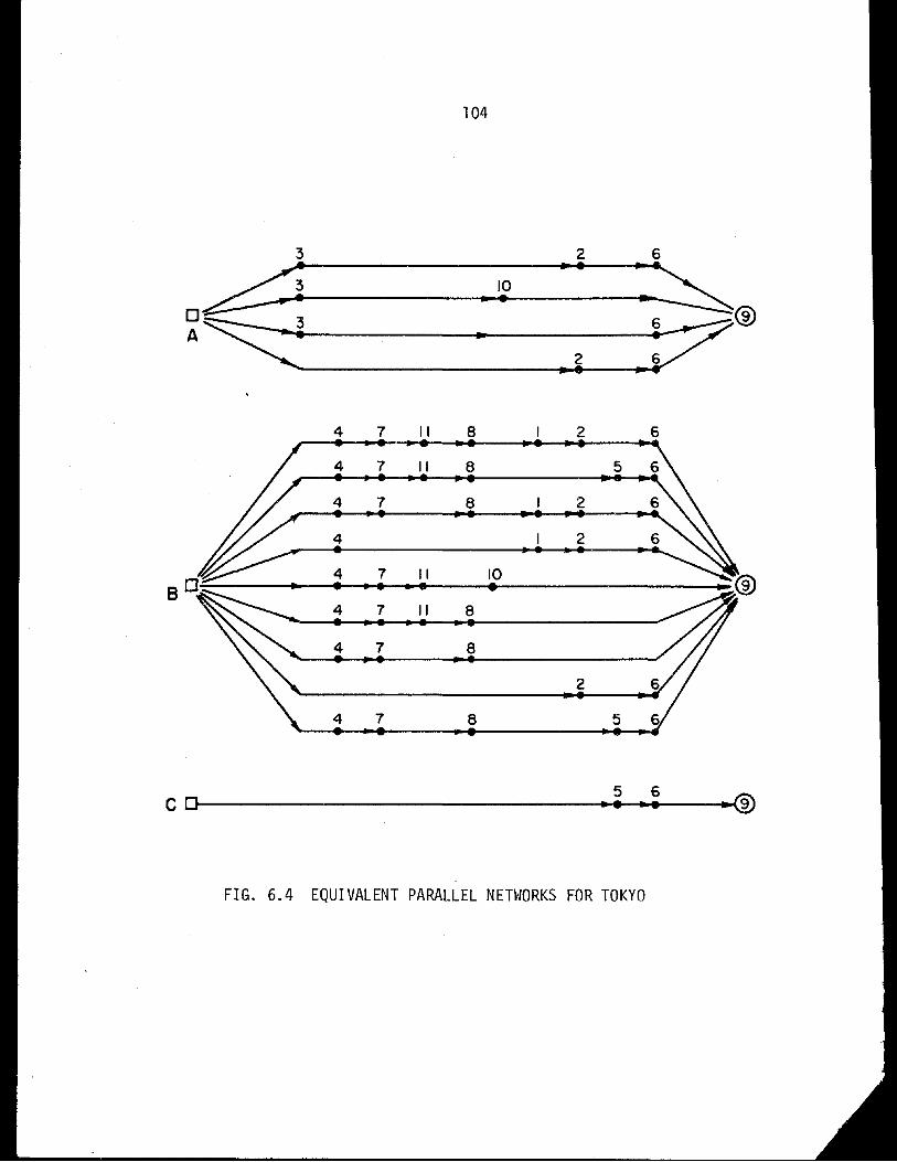
4 7 II 8 2 6
4 7 II 8 5
4 7 8 2
4 I 2• • • ....4 7 II 10• ... • • •4 7 II 8
4 7 8
2
4 7 8 5
104
FIG. 6.4 EQUIVALENT PARALLEL NETWORKS FOR TOKYO
3 2 6
d,., .~10...
~~ ... .~®2....
5 6c O~-----------------""''''''''.-'''''4.'''''---''''''®
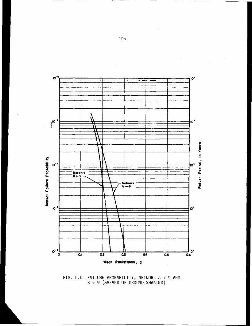
-----------
lit...i>-.5
c...:II..•a::
o'
10·
10'
0.50."0.5
105
Mecm Rni'tanco, 9
0.20.1
FIG. 6.5 FAILURE PROBABILITY, NETWORK A~ 9 ANDB ~ 9 (HAZARD OF GROUND SHAKING)
~
\\\\\,'\
N.twork8-9 ......... \
""" \
"" \ NetworkA-I
V
\I
I\\\\\
\ ~ I
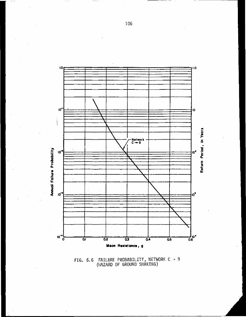
1.0
o'
10
.KJa ~
l-e:~•a:
0.50.4
106
0.30.20.1
FIG. 6.6 FAILURE PROBABILITY, NETWORK C ~ 9(HAZARD OF GROUND SHAKING)
J:)
I • \,~
"-\.
\\
N.tworky C-9
"""-
'"'\
"" I
""-
"''""10-'
°
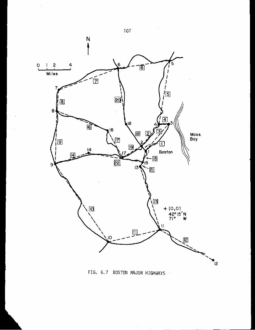
FIG. 6.7 BOSTON MAJOR HIGHWAYS
',,12
Mass.Bay
+ (0,0)42° 15
1N
71° W
I 5
II1Il[IDII
107
N
t
\\ [lg\
\\
\
\, ITJL ---\ 10 _----
4!
Miles
012I ! !

! ._. -
--··'7-----..:,",(7/"lIL •'''~
,
I
,,- 30'
FIG. 6.8 IMPORTANT EARTHQUAKES IN BOSTON AREA(REF. 49)
108
--------- -------------------------
cu.J,S-it ....
J ~.
41-30'_.._..._-- -_.__._-I
I '• , 4 i
~-+-_....-._--- ',1
IJ