A method for smoke marker measurements and its potential ... · of branches > straw > needles > leaves. ... populated areas, residential wood combustion, another form of biomass burning,

A method for smoke marker measurements and its potential

application for determining the contribution of biomass

burning from wildfires and prescribed fires to

ambient PM2.5 organic carbon

A. P. Sullivan,1 A. S. Holden,1 L. A. Patterson,1 G. R. McMeeking,1 S. M. Kreidenweis,1

W. C. Malm,2 W. M. Hao,3 C. E. Wold,3 and J. L. Collett Jr.1

Received 2 April 2008; revised 28 August 2008; accepted 5 September 2008; published 20 November 2008.

[1] Biomass burning is an important source of particulate organic carbon (OC)in the atmosphere. Quantifying this contribution in time and space requires a meansof routinely apportioning contributions of smoke from biomass burning to OC.Smoke marker (for example, levoglucosan) measurements provide the most commonapproach for making this determination. A lack of source profiles for wildfiresand prescribed fires and the expense and complexity of traditional smoke markermeasurement methods have thus far limited routine estimates of these contributionsto ambient aerosol concentrations and regional haze. We report here on the collectionof source profiles for combustion of numerous wildland fuels and on the developmentof an inexpensive and robust technique for routine smoke marker measurements.Hi-Volume filter source samples were collected during two studies at the FireScience Laboratory in Missoula, MT in 2006 and 2007. Levoglucosan (and othercarbohydrates) were measured in these samples using high-performance anion-exchangechromatography with pulsed amperometric detection. Results of this analysisalong with water-soluble potassium, OC, and elemental carbon are presented. The resultsshow that emissions of levoglucosan are fairly correlated with OC with an averageratio of 0.031 mg C/mg C. Further, there was a definite pattern that emergedbased on fuel component burned with the typical levoglucosan/OC ratioof branches > straw > needles > leaves. Additionally, this carbohydrate measurementmethod appears to provide fingerprint information about the type of fuel burnedthat could help constrain profiles chosen for aerosol source apportionment and leadto a better determination of source contributions from biomass burning.

Citation: Sullivan, A. P., A. S. Holden, L. A. Patterson, G. R. McMeeking, S. M. Kreidenweis, W. C. Malm, W. M. Hao, C. E. Wold,

and J. L. Collett Jr. (2008), A method for smoke marker measurements and its potential application for determining the contribution

of biomass burning from wildfires and prescribed fires to ambient PM2.5 organic carbon, J. Geophys. Res., 113, D22302,

doi:10.1029/2008JD010216.

1. Introduction

[2] One of the major sources of organic carbon aerosol isbiomass burning. Biomass burning smoke from wildfiresand prescribed fires can have a significant impact on PM2.5

concentrations, affecting air quality from local to regionaland global scales. This smoke can also be a significantcontributor in causing visibility impairment and affectingthe Earth’s radiation balance. In addition, there is evidence

in the Western U.S. for increased wildfires since the 1970sbecause of increased temperatures during the spring andsummer [Westerling et al., 2006]. The use of prescribedfire has also grown in recent decades in order to reducelarge accumulations of wildland fuel resulting from manydecades of an active fire suppression policy. In morepopulated areas, residential wood combustion, anotherform of biomass burning, can also be an important sourceof PM2.5. This all suggests that it is important to be able toroutinely apportion the contribution of biomass burning tothe total organic carbon aerosol concentrations.[3] One common approach to quantify the contribution

of biomass burning to the total organic carbon aerosol isthrough the use of smoke marker measurements. In thisapproach, a compound produced as part of the smokeemitted is monitored as the plume is transported down-wind and diluted. If the mass ratio of the marker to the

JOURNAL OF GEOPHYSICAL RESEARCH, VOL. 113, D22302, doi:10.1029/2008JD010216, 2008ClickHere

for

FullArticle

1Department of Atmospheric Science, Colorado State University, FortCollins, Colorado, USA.

2National Park Service/CIRA, Colorado State University, Fort Collins,Colorado, USA.

3USDA Forest Service, Fire Sciences Laboratory, Missoula, Montana,USA.

Copyright 2008 by the American Geophysical Union.0148-0227/08/2008JD010216$09.00

D22302 1 of 14

http://dx.doi.org/10.1029/2008JD010216

total organic carbon is known at the source and the markeris conserved during transport, then a measurement of themarker’s concentration at a downwind location can beused to determine the contribution of primary biomasssmoke to the total organic carbon.[4] This marker approach has been used by many inves-

tigators to apportion contributions of residential woodcombustion [e.g., Rogge et al., 1998] to urban particleconcentrations [e.g., Schauer et al., 1996; Schauer andCass, 2000; Fraser et al., 2003; Rinehart et al., 2006].However, few studies [e.g., Hays et al., 2002; Engling et al.,2006; Mazzoleni et al., 2007] have attempted to characterizeemissions by fuel types involved in wildfires or prescribedfires. Because of the lack of information available onemissions from wildfires and prescribed fires and the focusof most studies on urban settings, the results determined forthe contribution of biomass burning are generally moreskewed toward residential wood burning.[5] One of the most commonly used smoke markers is

levoglucosan, a sugar anhydride produced during the com-bustion of cellulose [Simoneit et al., 1999]. Water-solublepotassium has also been used as a less specific indicator ofbiomass burning contributions to ambient aerosols[Andreae, 1983]. While water-soluble potassium is oftenroutinely measured in aqueous extracts of filter-based aero-sol samples using cation-exchange chromatography, analy-sis of levoglucosan can be much more challenging.[6] Traditionally, levoglucosan in aerosol samples is

extracted and analyzed using a multi-step, labor-intensiveprocedure [Nolte et al., 2001; Hays et al., 2002; Zdrahal etal., 2002; Simpson et al., 2004]. In the first steps, the filtersare typically extracted in one or two organic solvents andthen the extracts are concentrated. The concentrated extractis next chemically derivatized by use of a silylating reagentto create silylesters for levoglucosan and other compoundsrelated to biomass burning (for example, mannosan andgalactosan). In the final step, the derivatized sample isanalyzed by Gas Chromatography/Mass Spectrometry(GC/MS). Overall, this analysis is quite labor intensiveand expensive because of the solvents, reagents, and instru-mentation needed. Therefore these analyses are generallyconducted only for selected filter samples from specialstudies or on composited filter samples.[7] All this information suggests there is a need for two

things in order to be able to obtain a better determination forthe contribution of wildfires and prescribed fires to the totalorganic carbon aerosol. One is an inexpensive and robustway to measure smoke marker compounds. Basically, thereis a need for a method to measure smoke markers that couldbe applied on a routine basis. The second is source profileinformation about smoke markers from relevant fire types(i.e., emission information from fuels known to be involvedin prescribed fires and wildfires).[8] In order to address the first need, an inexpensive and

robust technique that could be used for routine sampling hasbeen developed for measuring concentrations of levogluco-san and other carbohydrates in collected aerosol samples.This technique couples high-performance anion-exchangechromatography with pulsed amperometric detection(HPAEC-PAD). This approach offers numerous advantages,including extraction of the filter directly in water, the abilityto directly analyze the filter extract for levoglucosan, and

the use of ion chromatography (IC), an analytical platformalready in widespread use by aerosol monitoring networksfor analysis of the major inorganic aerosol species. UnlikeGC/MS this method does not detect other classes of biomassburning tracers such as resin acids or methoxyphenols orprovide mass spectra that can identify other known sourcemarkers. This technique has previously been applied tostudies of biomass combustion contributions to fine particlesin urban and rural settings as well as to source samples [Gaoet al., 2003;Gorin et al., 2006; Engling, 2006; Engling et al.,2006; Puxbaum et al., 2007].[9] The second need was addressed in the Fire Lab

at Missoula Experiment (FLAME). This was a multi-investigator study designed to collect chemical, physical,and optical property information about smoke by conductinga series of burn experiments at the United States ForestService Fire Science Laboratory (FSL) in Missoula, MT.The goal was to generate smoke source profiles that can beused to assess the contribution of wildfires and prescribedfires to the total organic carbon aerosol concentrations.With this in mind, fuels from key fire-prone areas, suchas the Western and Southeastern U.S., were tested duringFLAME I (May–June 2006) and FLAME II (May–June 2007).[10] In this paper, the application of an alternative

method to measure levoglucosan, along with measurementsof water-soluble potassium, organic carbon (OC), andelemental carbon (EC), to the source samples collectedduring FLAME I and II will be shown (i.e., the emissioninformation). Additional analysis of this data will bediscussed to show how these measurements can inform abetter determination of the impact of biomass burning.

2. Methods

2.1. Particulate Collection

[11] To collect ambient particles onto quartz filters foroff-line analysis a Thermo Anderson Hi-Volume AirSampler was used. A Hi-Volume Sampler was used so thatthe filter samples collected could be shared among multipleinvestigators. All samples were collected during the FLAMEI and II experiments conducted at the FSL in Missoula, MT.The FSL has a 12.5-m width� 12.5-m length� 22-m heightcombustion chamber where test burns of fuels relevant toprescribed fires and wildfires can be performed. More detailsabout the facility itself can be found in Christian et al.[2004].[12] Two different types of burns were conducted during

both FLAME campaigns: stack and chamber burns. In stackburns, the Hi-Volume Sampler was located on a measure-ment platform approximately 16 m above the ground, wherethe Hi-Volume Sampler was connected directly to the stackvia a sampling port designed by FSL. The fuel was burneddirectly under the 1.5-m diameter stack, and the emissionswere forced up the stack because of the positive air pressureinside the chamber that was vented through the stack. Stackburns were generally short in duration and lasted anywherefrom a few to 30 minutes. Therefore stack burns weregenerally conducted in duplicate or triplicate for a particularfuel and one Hi-Volume filter sample was collected acrossthe whole series of replicates.[13] For chamber burns, the fuel bed was placed about 5 m

from the stack and the smoke was allowed to completely fill

D22302 SULLIVAN ET AL.: A METHOD FOR SMOKE MARKER MEASUREMENTS

2 of 14

D22302

the entire burn chamber (i.e., there was no stack flow duringthese burns). The Hi-Volume Sampler was placed on thefloor of the chamber and collected a sample directly fromthe smoke that filled the entire burn chamber. Chamberburns were generally longer in duration than the stack burns,lasting anywhere from 1.5 to 2 hours. One Hi-Volume filtersample was collected across each chamber burn.[14] For both types of burns the fuel bed continuously

sat on top of a balance, allowing for determination of thetotal amount of fuel consumed. During FLAME I the burnswere ignited by either a butane lighter or propane torch. Totry and allow for more even heating during FLAME II, thiswas switched to having the fuel itself sit on top of heatingtapes wetted with ethanol. At the beginning of a burn avariac, which controlled the heating of the tapes, wasturned on until the fuel was ignited. No noticeable differ-ences were observed in parameters reported here as a resultof making this switch and therefore data collected fromboth ignition methods will be presented.[15] The Hi-Volume Sampler used for both the stack and

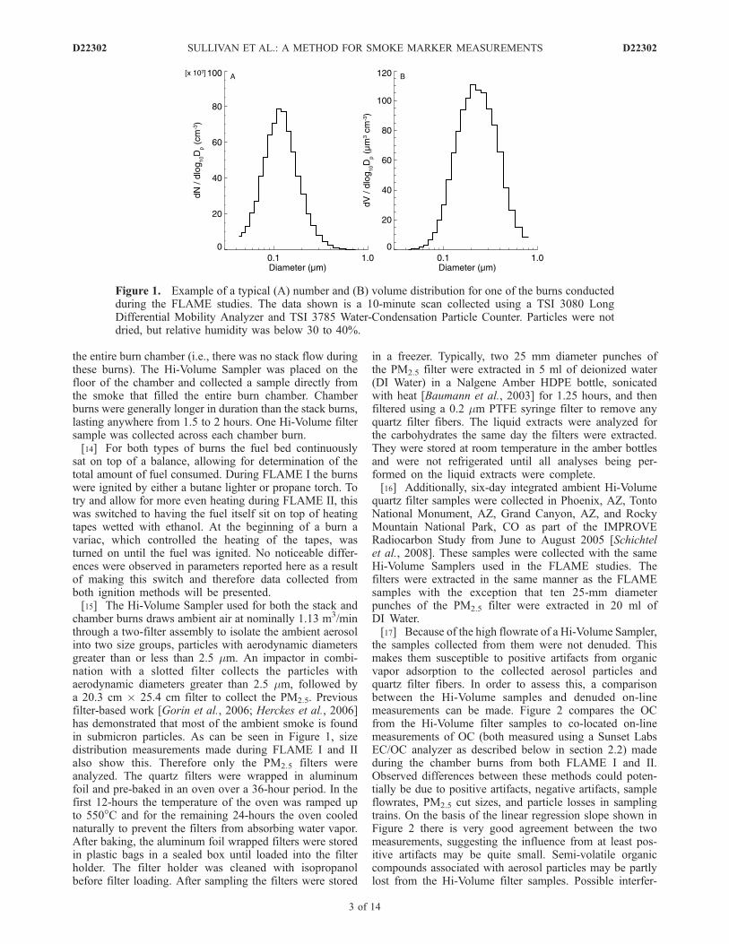
chamber burns draws ambient air at nominally 1.13 m3/minthrough a two-filter assembly to isolate the ambient aerosolinto two size groups, particles with aerodynamic diametersgreater than or less than 2.5 mm. An impactor in combi-nation with a slotted filter collects the particles withaerodynamic diameters greater than 2.5 mm, followed bya 20.3 cm � 25.4 cm filter to collect the PM2.5. Previousfilter-based work [Gorin et al., 2006; Herckes et al., 2006]has demonstrated that most of the ambient smoke is foundin submicron particles. As can be seen in Figure 1, sizedistribution measurements made during FLAME I and IIalso show this. Therefore only the PM2.5 filters wereanalyzed. The quartz filters were wrapped in aluminumfoil and pre-baked in an oven over a 36-hour period. In thefirst 12-hours the temperature of the oven was ramped upto 550�C and for the remaining 24-hours the oven coolednaturally to prevent the filters from absorbing water vapor.After baking, the aluminum foil wrapped filters were storedin plastic bags in a sealed box until loaded into the filterholder. The filter holder was cleaned with isopropanolbefore filter loading. After sampling the filters were stored

in a freezer. Typically, two 25 mm diameter punches ofthe PM2.5 filter were extracted in 5 ml of deionized water(DI Water) in a Nalgene Amber HDPE bottle, sonicatedwith heat [Baumann et al., 2003] for 1.25 hours, and thenfiltered using a 0.2 mm PTFE syringe filter to remove anyquartz filter fibers. The liquid extracts were analyzed forthe carbohydrates the same day the filters were extracted.They were stored at room temperature in the amber bottlesand were not refrigerated until all analyses being per-formed on the liquid extracts were complete.[16] Additionally, six-day integrated ambient Hi-Volume

quartz filter samples were collected in Phoenix, AZ, TontoNational Monument, AZ, Grand Canyon, AZ, and RockyMountain National Park, CO as part of the IMPROVERadiocarbon Study from June to August 2005 [Schichtelet al., 2008]. These samples were collected with the sameHi-Volume Samplers used in the FLAME studies. Thefilters were extracted in the same manner as the FLAMEsamples with the exception that ten 25-mm diameterpunches of the PM2.5 filter were extracted in 20 ml ofDI Water.[17] Because of the high flowrate of a Hi-Volume Sampler,

the samples collected from them were not denuded. Thismakes them susceptible to positive artifacts from organicvapor adsorption to the collected aerosol particles andquartz filter fibers. In order to assess this, a comparisonbetween the Hi-Volume samples and denuded on-linemeasurements can be made. Figure 2 compares the OCfrom the Hi-Volume filter samples to co-located on-linemeasurements of OC (both measured using a Sunset LabsEC/OC analyzer as described below in section 2.2) madeduring the chamber burns from both FLAME I and II.Observed differences between these methods could poten-tially be due to positive artifacts, negative artifacts, sampleflowrates, PM2.5 cut sizes, and particle losses in samplingtrains. On the basis of the linear regression slope shown inFigure 2 there is very good agreement between the twomeasurements, suggesting the influence from at least pos-itive artifacts may be quite small. Semi-volatile organiccompounds associated with aerosol particles may be partlylost from the Hi-Volume filter samples. Possible interfer-

Figure 1. Example of a typical (A) number and (B) volume distribution for one of the burns conductedduring the FLAME studies. The data shown is a 10-minute scan collected using a TSI 3080 LongDifferential Mobility Analyzer and TSI 3785 Water-Condensation Particle Counter. Particles were notdried, but relative humidity was below 30 to 40%.


3 of 14

D22302

ences from the filter’s background were found to benegligible on pre-baked Hi-Volume quartz filters set asideas blanks during both types of burns.

2.2. Measurement Approach

[18] Each of the Hi-Volume filters collected was analyzedindividually for PM2.5 levoglucosan, water-soluble potassium(K+), OC, and EC. These analyses are described below.The levoglucosan method is described in detail since amodified version of the original method discussed inEngling et al. [2006] is being used here. The modificationsmade to the levoglucosan method were done to help inshortening the run time and had no effect on the responsefor levoglucosan.[19] After each filter was extracted the aqueous sample

was analyzed for levoglucosan (and various other carbohy-drates) using high-performance anion-exchange chromatog-raphy with pulsed amperometric detection (HPAEC-PAD)and for K+ using IC.[20] The levoglucosan measurement was made using a

Dionex DX-500 series ion chromatograph with a DionexGP-50 gradient pump and Dionex ED-50 electrochemicaldetector operating in integrating amperometric mode usingwaveform A. The electrochemical detector is connected to aDionex ED-50/ED-50A electrochemical cell, which con-tains a ‘‘standard’’ gold working electrode and pH-Ag/AgCl(silver/silver chloride) reference electrode.[21] In HPAEC-PAD once the analytes are eluted from

the column they enter an electrochemical cell where they areelectroanalytically oxidized on the surface of a gold work-ing electrode by applying a positive potential. However, ifthis continued to happen, the electrode surface would bepoisoned by the oxidation products. To prevent this fromhappening, an entirely different potential is applied to cleanthe surface of the electrode. PAD is essentially the repeatedapplication of this whole series of potentials, referred to as awaveform.

[22] The eluents are DI Water and 200 mM sodiumhydroxide (NaOH). In order to minimize carbonate ions inthe eluents, which can be a potential interference, theeluents are continuously degassed with ultra high purityhelium. In addition, the 200 mM NaOH is made from50% w/w NaOH and allowed to equilibrate overnightbefore using for analysis.[23] Separation was completed on Dionex CarboPac

PA-10 guard (4 � 50 mm) and analytical (4 � 250 mm)columns. Each run has an eluent flowrate of 0.5 ml/minand takes approximately 54 minutes. For the first 10 minutesisocratic elution with 18 mM NaOH is performed to detectanhydrosugars such as levoglucosan and mannosan. Next,a linear gradient from 18 to 60 mM NaOH is run for14 minutes to detect sugars such as galactose, mannose, andglucose. Since carbonate ions can bind to the active sites ofthe resin and affect the chromatography, the column iscleaned for 14 minutes with 180 mM NaOH. Finally, a16-minute re-equilibration step is performed to return to thestarting conditions. Generally a sample volume of 50 mL isinjected onto the column.[24] The method is capable of readily separating a mix of

common carbohydrates, including sugars glucose and man-nose along with the anhydrosugars that are recognized asimportant chemical constituents of wood smoke. We wouldpoint out that this method is not capable of separating thesugar alcohols (for example, arabitol and mannitol) from theanhydrosugars. This means that arabitol can potentiallyoverlap with levoglucosan and mannitol with mannosan.However, for these source samples this was found not to bean issue as we have additionally run them on a DionexCarboPac PA-1 column which can completely resolvemannitol and mannosan and partially resolve arabitol andlevoglucosan [Caseiro et al., 2007]. Sugar alcohols could bea factor in ambient samples as both have been detected asindicators of fungal spores for samples collected in Vienna,Austria [Bauer et al., 2008a, 2008b].[25] A sample calibration chromatogram using the

CarboPac PA-10 column method described is shown inFigure 3. The anhydrosugars are detected in the first tenminutes and the sugars at around 25 minutes. Calibrationsare linear over a wide concentration range and the methodis extremely sensitive. Measurements of levoglucosan bythis approach have been compared with measurements byboth GC/MS and LC/MS (liquid chromatography/massspectroscopy) with good results [Engling et al., 2006].The limit of detection (LOD) for the various carbohydratesis less than approximately 0.10 mg/m3 (or 2.26 mg). Itshould be noted that all the LODs listed in this section arefor only this particular data set and were calculatedassuming a flowrate of 1.13 m3/min and sampling timeof 20 min, the average sampling time during stack burns.Lower LODs have easily been achieved for all the meas-urements with an increased integration time more typical ofambient filter samples.[26] Water-soluble potassium was measured in the liquid

extract using a Dionex DX-500 series ion chromatographwith a Dionex CD-20 conductivity detector, Dionex IP-20isocratic pump, and self-regenerating cation SRS-ULTRAsuppressor. A Dionex IonPac CS12A analytical (3 �150 mm) column, with a sample volume injection of 25 mL,was used to achieve separation of the common inorganic

Figure 2. Comparison of the non-denuded Hi-Volumefilter OC and the denuded on-line OC. Both measurementswere made using a Sunset EC/OC analyzer. Uncertaintieswith the least square regression are one standard deviation.


4 of 14

D22302

cations in 15 minutes. A 20-mMmethanesulfonic acid eluentat a flowrate of 0.5 ml/min was used. The LOD for water-soluble potassium is about 0.36 mg/m3.[27] Organic and elemental carbon were determined

using a Sunset Labs EC/OC semi-continuous analyzer(Forest Grove, Oregon). It quantifies OC and EC carbonmass by thermal/optical transmission (TOT) [Birch andCary, 1996]. The instrument was operated following theNIOSH Method 5040 [Eller and Cassinelli, 1996]. Eachfilter was analyzed by running the analyzer in off-linemode. The average concentration determined from two1.4 cm2 filter punches was used. The LODs for OC andEC in a 20 minute Hi-Volume sample are approximately6.0 mg C/m3 and 1.0 mg C/m3, respectively. For the on-linemeasurements, the instrument was run continuously with a20-minute collection time. The LODs for the on-linemeasurements are 0.2 mg C/m3 and 0.5 mg C/m3 for OCand EC, respectively.

3. Results and Discussion

[28] During FLAME I and II approximately 252 burnsinvolving 30 different fuels were tested. These experimentsincluded either burning a single component of a fuel (forexample, branches only), a mixture of components of a fuel(for example, leaves and branches together), or a mixture ofmore than one type of fuel. The data analysis presented insections 3.1 and 3.2 focuses mainly on the experimentsinvolving the burning of a single fuel component.[29] Table 1 lists the various burn experiments performed

along with the observed carbohydrate, water-soluble potas-sium, OC, and EC concentrations. Levoglucosan wasmeasured in all the fuels tested. The anhydrosugars appearin higher concentrations than the sugars, with levoglucosanbeing the dominant carbohydrate observed. Water-solublepotassium was observed in most of the burns. At timeswater-soluble potassium could be found in higher concen-trations than levoglucosan. OC was observed in all the fuelstested; however, EC was not. Although generally OCconcentrations were much higher than EC concentrations,there were some fuels that emitted considerable amounts ofEC (for example, Chamise). Although the absolute concen-trations are being shown, it should be noted that the focus

should be on the relative amounts of the different speciessince the absolute concentration can depend on the amountof fuel burned, the burn rate, and for stack burns potentiallythe flowrate of air up the stack. Therefore Table 1 alsocontains data for the total mass of fuel burned, the stack andHi-Volume Sampler flowrates, and sampling time for eachof the burns so the ratios of any of the measured species tothe fuel burned could be examined. The work presentedhere in the next section will, however, focus on the ratios oflevoglucosan to OC and water-soluble potassium.

3.1. Correlation of Levoglucosan to OCand Water-Soluble Potassium

[30] Figure 4a shows levoglucosan vs. OC on a carbonmass basis for the individual fuel component burnspresented in Table 1. Table 2 lists the levoglucosan toOC ratios for this subset of data. This subset of data includes73 burns, 7 of which are for grasses, 10 for branches, 7 forduffs, 10 for needles, 7 for straw, and 32 for leaves.[31] There is an overall correlation between levoglucosan

and OC (R2 = 0.68) as can be seen in Figure 4a. Althoughthese two measurements are correlated, the fraction of OCmade up of levoglucosan is actually small, as indicated bya slope forced through zero of 0.023 mg C/mg C (0.052 mglevoglucosan/mg OC).[32] The data are segregated by fuel component burned in

Figure 4b. A pattern in the levoglucosan to OC ratioemerges. The levoglucosan and OC are highly correlatedfor branches, straw, needles, and leaves, with branchesgenerally having the highest average ratio. However, forduffs and grasses the levoglucosan is poorly correlated withthe OC.[33] The observed pattern in levoglucosan to OC ratios

for fuel components is similar to the cellulose to hemicel-lulose ratio presented in a review paper by Hoch [2007](see Figure 1 of this reference). While hemicellulosecontents of these biomass components are similar, cellulosecontents vary. Components with higher cellulose content(for example, branches) are found to yield higher levoglu-cosan to OC ratios. This is not surprising since levoglu-cosan is a product of thermal degradation of cellulose.[34] Although there is a pattern in the levoglucosan to OC

ratio based on fuel component, as can be seen in Figure 5

Figure 3. Calibration chromatogram for the injection of a mixed carbohydrate standard using theHPAEC-PAD method, where Tr is retention time.


5 of 14

D22302

Table

1.Carbohydrate

Concentrations,Water-Soluble

Potassium

Concentration,OC

Concentration,EC

Concentration,Stack

Flowrate,Hi-VolumeSam

plerFlowrate,Sam

plingTim

e,and

MassofFuelBurned

fortheVariousBurn

Experim

ents,WhereND=ConcentrationnotDetectedorStack

FlowrateCould

notbeDetermined,I=MeasuredDuringFLAMEI,II=Measured

DuringFLAMEII,s=Stack

Burn,c=Cham

ber

Burn,G

=Grass,B=branches,D

=Duff,N

=Needles,S=Straw

,L=Leaves,andNL=Needle

Littera

Fuel

Levoglucosan

(mg/m

3)

Mannosan

(mg/m

3)

Galactosan

(mg/m

3)

Galactose

(mg/m

3)

Glucose

(mg/m

3)

Mannose

(mg/m

3)

Water-Soluble

Potassium

(mg/m

3)

OC

(mgC/m

3)

EC

(mgC/m

3)

Stack

Flowrate

(m3/m

in)

Hi-Volume

Flowrate

(m3/m

in)

Sam

pling

Tim

e(m

in)

Mass

Burned

(g)

Commentb

IndividualComponent

Alaskan

Duff

12.59

11.60

7.07

ND

ND

ND

2.20

126.42

ND

1.13

118.00

58.0

II,c,

D14.67

6.32

2.11

ND

ND

ND

ND

95.89

ND

1.10

88.00

19.4

II,c,

D23.71

17.79

10.46

ND

ND

ND

1.09

182.14

ND

414.6

1.08

38.88

181.7

II,s,D

14.46

14.64

8.04

ND

ND

ND

1.12

166.45

ND

1.22

120.00

96.1

I,c,

DBlack

Needle

Rush

(FL)

6.66

0.51

0.50

ND

ND

ND

12.21

83.57

3.27

1.10

88.00

45.5

II,c,

GBlack

Spruce

(AK)

5.64

1.35

0.42

ND

ND

ND

1.05

77.29

24.11

1.08

118.00

62.5

II,c,

NBlack

Spruce,dried

(AK)

25.53

8.32

2.89

ND

0.12

ND

4.66

309.40

26.87

336.0

1.15

28.00

438.8

II,s,N

Black

Spruce,fresh(A

K)

28.32

6.72

2.80

ND

0.19

ND

4.37

359.43

3.67

339.0

1.15

18.00

469.7

II,s,N

Ceanothus(CA)

9.95

0.68

0.75

ND

0.20

ND

75.65

184.15

29.06

436.8

1.18

14.00

442.3

II,s,L

7.64

0.34

0.65

ND

ND

ND

20.10

147.69

5.75

1.25

119.00

181.4

I,c,

LCham

ise(CA)

1.60

0.22

0.17

ND

ND

ND

19.86

43.60

43.98

ND

1.10

88.00

95.4

II,c,

L8.16

0.79

0.84

ND

0.17

ND

56.77

189.76

49.16

1.16

15.00

328.0

II,s,L

Cham

ise,

dried

(CA)

20.32

0.81

2.89

ND

0.19

ND

46.36

320.15

5.18

397.8

1.03

30.35

684.0

I,s,L

1.97

0.34

0.19

ND

ND

ND

26.92

44.66

61.98

1.22

125.00

186.2

I,c,

LCham

ise,

dried

(CA)

6.81

0.97

0.61

ND

ND

ND

1.67

64.90

ND

375.6

1.03

60.97

506.9

I,s,B

Cham

ise,

fresh(CA)

21.98

0.93

3.48

0.06

ND

ND

35.37

380.53

ND

395.4

1.03

36.04

630.1

I,s,L

Cham

ise,

fresh(CA)

6.19

1.00

0.60

ND

ND

ND

2.36

60.22

ND

387.0

1.03

59.19

571.1

I,s,B

Fir,dried

(MT)

4.76

1.64

1.24

ND

ND

ND

0.70

180.22

ND

ND

1.19

36.00

99.2

II,s,N

Fir,dried

(MT)

12.51

2.96

3.34

ND

0.12

ND

1.78

172.83

ND

437.4

1.16

16.00

196.0

II,s,B

Fir,fresh(M

T)

30.84

8.94

7.44

ND

0.69

0.10

2.95

631.78

ND

337.2

1.16

46.00

325.0

II,s,N

Gallberry

(MS)

1.53

ND

0.13

ND

ND

ND

8.69

52.43

51.89

337.8

1.10

88.00

44.7

II,c,

L13.52

0.62

1.13

ND

0.17

ND

57.08

370.70

425.20

1.02

12.50

401.2

II,s,L

Grass,dried

(MT)

8.73

0.62

0.74

ND

ND

ND

29.34

219.77

10.89

417.6

0.98

16.42

126.2

I,s,G

Grass,fresh(M

T)

4.77

0.52

0.51

ND

0.11

ND

58.51

225.44

ND

404.4

0.98

32.70

243.6

I,s,G

Hickory

(NC)

10.83

1.14

2.21

ND

0.18

ND

27.22

290.35

12.38

336.0

1.13

11.00

193.9

II,s,L

Juniper

(UT)

0.78

0.23

0.16

ND

ND

ND

14.56

52.70

182.06

1.13

112.00

197.3

I,c,

LKudzo

(GA)

18.04

7.57

1.72

ND

0.23

ND

16.04

711.31

ND

331.2

1.10

11.00

173.4

II,s,L

Lodgepole

PineNeedle

Duff(M

T)

9.87

5.86

2.25

ND

ND

ND

ND

73.55

ND

404.4

1.01

88.61

455.9

I,s,D

Lodgepole

Pine,

dead/small(M

T)

9.74

2.68

1.34

ND

ND

ND

0.70

52.39

54.60

433.8

1.01

42.75

675.2

I,s,B

Lodgepole

Pine,

fresh(M

T)

12.70

8.97

4.88

ND

0.26

ND

5.53

240.20

1.14

430.2

1.01

94.47

504.3

I,s,N

Longleaf

Pine(M

S)

25.01

14.25

5.19

ND

0.13

ND

7.19

345.94

14.67

353.4

1.12

43.00

401.9

II,s,N

Manzanita(CA)

27.54

1.13

2.27

ND

0.20

ND

26.02

315.27

21.06

436.2

1.16

16.00

471.2

II,s,L

4.74

0.38

0.38

ND

ND

ND

15.46

59.14

47.70

1.26

110.00

192.8

I,c,

LManzanita,

dried

(CA)

15.08

0.28

5.16

ND

0.17

ND

6.90

476.74

2.16

377.4

1.01

87.45

685.5

I,s,L

Manzanita,

fresh(CA)

14.49

0.30

3.15

ND

0.13

ND

7.28

294.83

ND

ND

1.03

73.67

547.2

I,s,L

Manzanita,

fresh(CA)

24.03

3.72

4.25

ND

0.16

ND

6.21

213.46

ND

398.4

1.03

30.13

673.1

I,s,B

Oak

(NC)

24.57

1.98

4.53

ND

0.17

ND

24.80

394.18

14.99

353.4

1.13

11.50

218.2

II,s,L

Palmetto

(FL)

3.35

0.34

0.39

ND

ND

ND

126.30

86.69

27.72

393.6

1.03

26.57

693.5

I,s,L

5.03

0.48

0.27

ND

ND

ND

14.02

75.17

16.75

1.22

125.00

187.0

I,c,

LPalmetto

(FLcoastal)

24.00

1.39

1.03

ND

0.18

ND

37.89

323.26

38.27

338.4

1.10

14.50

469.6

II,s,L

0.62

0.12

ND

ND

ND

ND

6.85

25.78

34.53

1.13

118.00

91.0

II,c,

LPalmetto

(FLinland)

19.31

1.37

1.50

ND

0.14

ND

22.66

417.91

63.66

ND

1.08

15.50

451.4

II,s,L

Palmetto

(MS)

28.83

1.73

1.80

ND

0.17

ND

18.81

361.24

23.02

345.6

1.13

120.00

458.5

II,s,L

2.35

0.18

0.11

ND

ND

ND

4.86

40.55

13.49

1.09

14.00

87.5

II,c,

LPhragmites

(LA)

16.85

0.92

1.59

ND

0.33

0.14

4.44

224.08

4.29

355.2

1.13

10.50

101.8

II,s,G


6 of 14

D22302

Table

1.(continued)

Fuel

Levoglucosan

(mg/m

3)

Mannosan

(mg/m

3)

Galactosan

(mg/m

3)

Galactose

(mg/m

3)

Glucose

(mg/m

3)

Mannose

(mg/m

3)

Water-Soluble

Potassium

(mg/m

3)

OC

(mgC/m

3)

EC

(mgC/m

3)

Stack

Flowrate

(m3/m

in)

Hi-Volume

Flowrate

(m3/m

in)

Sam

pling

Tim

e(m

in)

Mass

Burned

(g)

Commentb

Ponderosa

PineDuff

8.41

4.37

2.27

ND

ND

ND

0.37

110.24

1.40

404.4

1.01

82.53

456.0

I,s,D

11.94

11.97

4.49

ND

ND

ND

0.70

195.98

1.12

1.30

119.00

107.2

I,c,

DPonderosa

Pine,

dead/large(M

T)

6.35

1.80

1.41

ND

ND

ND

0.57

49.86

38.05

359.4

1.01

64.19

706.3

I,s,B

Ponderosa

Pine,

dead/small(M

T)

5.41

1.26

1.09

ND

ND

ND

0.61

69.92

57.11

385.2

1.01

50.38

385.5

I,s,B

Ponderosa

Pine,

fresh(M

T)

8.73

2.10

1.44

ND

ND

ND

1.66

100.60

ND

362.4

1.01

124.03

612.1

I,s,N

Ponderosa

Pine,

fresh/large(M

T)

7.80

1.84

1.06

ND

ND

ND

0.78

87.58

ND

345.6

1.00

44.67

212.2

I,s,B

Ponderosa

Pine,

fresh/small(M

T)

11.80

11.12

5.04

ND

0.18

ND

2.04

334.00

ND

356.4

1.00

57.00

497.3

I,s,B

Puerto

Rican

Fern

10.13

9.17

1.46

ND

ND

ND

7.46

144.63

8.34

1.27

127.00

173.9

I,c,

LPuerto

Rican

Mixed

Woods

7.30

0.62

0.26

ND

ND

ND

1.47

56.79

5.88

1.25

130.00

83.8

I,c,

BRhododendron(N

C)

6.89

0.57

0.55

ND

ND

0.01

3.94

68.38

6.88

1.10

118.00

94.8

II,c,

LRiceStraw

(Taiwan)

1.97

0.16

0.15

ND

0.02

ND

6.84

33.34

ND

1.13

118.50

79.6

II,c,

S28.76

1.53

2.30

0.12

0.25

0.11

39.49

550.67

ND

429.6

1.10

13.73

438.0

II,s,S

33.02

0.60

3.43

ND

0.16

ND

36.29

363.69

ND

400.2

1.01

23.79

514.3

I,s,S

12.02

0.85

1.00

ND

0.13

0.11

25.26

182.01

10.04

435.0

1.03

13.00

202.0

I,s,S

25.69

0.76

1.77

ND

0.17

0.13

21.09

290.97

ND

ND

1.03

11.58

164.3

I,s,S

25.05

0.81

1.84

ND

0.16

0.14

38.58

321.74

ND

413.4

1.03

10.50

215.8

I,s,S

7.44

0.15

0.40

ND

ND

ND

25.66

74.59

1.63

1.32

116.00

172.9

I,c,

SSage(M

T)

28.33

6.51

4.59

0.11

0.28

0.11

96.33

690.01

19.73

398.4

1.08

19.03

452.7

II,s,L

Sage(U

T)

4.57

1.23

0.77

ND

ND

ND

26.20

308.32

5.27

471.6

1.16

9.00

122.0

II,s,L

Saw

Grass

(LA)

18.88

1.64

1.81

ND

0.17

ND

301.98

462.45

57.45

407.4

1.12

11.25

273.2

II,s,G

SouthernPine,

dried

10.53

6.42

1.34

ND

ND

ND

1.07

107.42

7.29

1.27

117.00

72.8

I,c,

NTiti(FL)

6.40

0.62

0.55

ND

0.13

ND

26.84

126.61

43.37

ND

1.15

16.00

255.8

II,s,L

Turkey

Oak

(NC)

52.87

3.60

12.48

ND

0.18

ND

60.72

1124.38

50.07

427.2

1.08

20.00

485.6

II,s,L

Wax

Myrtle

(FL)

7.07

1.59

1.23

ND

ND

ND

24.93

126.79

16.60

1.30

125.00

152.9

I,c,

LWax

Myrtle

(MS)

18.92

1.34

2.16

ND

0.16

ND

41.27

320.92

12.29

351.6

1.13

18.50

336.1

II,s,L

WhiteSpruce

(AK)

7.31

1.35

0.43

ND

ND

ND

3.14

55.07

ND

1.13

88.00

36.9

II,c,

NWiregrass

(FL)

7.98

0.36

0.21

ND

ND

ND

0.84

39.75

2.62

1.10

88.00

44.7

II,c,

GWiregrass

(MS)

20.36

0.52

0.41

ND

0.12

ND

2.25

118.48

11.59

328.2

1.10

19.00

207.6

II,s,G

ComponentMixtures

Cham

ise(CA)

2.66

0.24

0.42

ND

ND

ND

29.85

73.42

35.16

403.8

1.01

32.47

690.5

I,s,L,B

1.61

0.12

0.15

ND

ND

ND

20.82

31.60

64.11

1.30

114.83

282.4

I,c,

L,B

Fir,dried

(MT)

3.68

1.00

0.83

ND

ND

ND

0.46

98.58

ND

436.2

1.13

103.00

82.6

II,c,

N,B

2.23

0.61

0.36

ND

ND

ND

1.96

86.66

ND

1.13

88.00

23.5

II,c,

N,B

6.34

1.90

1.87

ND

ND

ND

0.79

131.44

ND

1.13

56.00

201.0

II,s,N,B

Fir,fresh(M

T)

2.53

0.51

0.30

ND

ND

ND

6.84

57.03

27.46

388.2

1.08

126.00

95.7

II,c,

N,B

45.64

9.32

7.85

ND

0.84

0.12

9.50

675.45

2.95

1.16

24.00

433.6

II,s,N,B

Lodgepole

Pine(M

T)

13.40

12.32

6.03

ND

ND

ND

0.45

160.83

9.75

ND

1.03

105.96

610.9

I,s,NL

Lodgepole

Pine,

dried

(MT)

15.72

11.28

4.53

ND

ND

ND

0.58

212.63

14.33

1.25

93.00

147.5

I,c,

N,B

Ponderosa

Pine(M

T)

21.05

14.15

6.17

ND

0.12

ND

1.20

312.11

6.11

405.0

1.00

52.77

682.8

I,s,NL

41.52

40.15

14.98

ND

0.17

ND

1.91

678.81

ND

420.6

1.01

30.34

634.9

I,s,NL

23.48

17.62

6.23

ND

0.11

ND

1.35

285.23

6.39

415.2

1.01

44.44

655.3

I,s,NL

25.15

18.22

8.13

ND

0.10

ND

1.12

335.40

1.55

ND

1.01

52.02

636.2

I,s,NL

25.74

18.13

8.11

ND

ND

ND

0.93

364.61

2.69

412.8

1.01

50.45

668.0

I,s,NL

Ponderosa

Pine,

dried

(MT)

10.48

5.58

1.54

ND

ND

ND

0.61

143.42

8.39

1.33

117.25

103.9

I,c,

N,B

19.41

23.20

9.66

ND

0.18

ND

0.71

541.06

45.38

1.30

94.67

184.6

I,c,

N,B


7 of 14

D22302

and Table 2, the majority of the ratios for all fuels fallbetween 0.005 and 0.060 mg C/mg C (0.011 and 0.135 mglevoglucosan/mg OC), with an average ratio and standarddeviation of 0.031 ± 0.017 mg C/mg C (0.070 ± 0.038 mglevoglucosan/mg OC). When comparing this range of ratiosto literature values, it appears that a larger range in ratios isgenerally observed for residential wood burning. For exam-ple, Schauer et al. [2001], which focused on residentialwood burning, found a range of ratios for the three fuelstested of 0.060 to 0.230 mg C/mg C (0.135 mg levoglucosan/mg OC). Fine et al. [2004], which also focused on residen-tial wood burning, found ratios that ranged from 0.004 to0.148 mg C/mg C (0.010 to 0.334 mg levoglucosan/mg OC)when testing 10 fuels. However, for a study more similar to

Table

1.(continued)

Fuel

Levoglucosan

(mg/m

3)

Mannosan

(mg/m

3)

Galactosan

(mg/m

3)

Galactose

(mg/m

3)

Glucose

(mg/m

3)

Mannose

(mg/m

3)

Water-Soluble

Potassium

(mg/m

3)

OC

(mgC/m

3)

EC

(mgC/m

3)

Stack

Flowrate

(m3/m

in)

Hi-Volume

Flowrate

(m3/m

in)

Sam

pling

Tim

e(m

in)

Mass

Burned

(g)

Commentb

Fuel

Mixtures

Black

Needle

Rush

andSaltMarsh

Grass

(NC)

57.59

3.07

7.49

ND

0.36

ND

151.08

684.55

11.08

424.8

1.10

16.02

458.9

II,s,G,G

Hickory

andOak

(NC)

4.96

0.51

0.84

ND

ND

ND

15.21

115.03

10.52

ND

1.16

125.00

93.2

II,c,

L,L

17.17

1.23

3.06

0.20

0.22

ND

15.43

334.19

ND

1.15

13.00

236.7

II,s,L,L

Longleaf

PineandWiregrass

12.50

10.10

2.75

ND

ND

ND

8.39

189.75

8.84

1.13

133.00

114.0

II,c,

N,G

Longleaf

PineandWiregrass

(MS)

18.45

4.19

1.79

ND

0.11

ND

2.54

137.62

ND

317.4

1.14

58.50

399.6

II,s,N,G

Palmetto

andGallberry

(MS)

36.17

2.87

3.61

0.21

0.28

ND

17.48

500.02

ND

336.6

1.13

28.50

443.4

II,s,L,L

Rabbitbrush

andSage(U

T)

2.10

0.40

0.21

ND

ND

ND

58.52

53.01

111.70

1.23

60.00

182.8

I,c,

L,L

aThetableisseparated

into

threesections:individualcomponentburns,burnsinvolvingamixtureofcomponents,andburnsinvolvingamixture

ofdifferenttypes

offuels.Ifavailable,in

parenthesisbythefuelnam

eisthelocationfrom

wherethefuel

was

obtained.

bFortheindividualcomponentburnsthereareatotalof7forgrasses,10forbranches,7forduffs,10forneedles,7forstraw,and32forleaves.Fortheburnsinvolvingamixture

ofcomponentsthereareatotalof2

forleaf

andbranch

mixtures,8forneedleandbranch

mixtures,and6forneedlelitter.Fortheburnsinvolvingamixtureofdifferentfuelsthereareatotalof1withtwotypes

ofgrasses,4withtwotypes

ofleaves,and2

withneedlesmixed

withgrasses.

Figure 4. Correlation between levoglucosan and OC on acarbon mass basis forced through zero for (a) all the data and(b) with the data segregated by fuel component for all theexperiments involving the burning of a single component offuel. Branches are in purple, straw in black, duffs in pink,needles in red, leaves in green, and grasses in blue.Uncertainties with the least square regression are onestandard deviation. N indicates the number of samplesanalyzed for each of the six different fuel components burned.


8 of 14

D22302

FLAME, conducted by Hays et al. [2002] using a burnenclosure, a range of ratios from 0.016 to 0.025 mg C/mg C(0.036 to 0.056 mg levoglucosan/mg OC) was found whentesting six different fuels.[35] The levoglucosan to OC ratios obtained for Ponder-

osa Pine from FLAME can also be compared to literaturevalues. Schauer et al. [2001], who did not specify the type

of pine burned, and Fine et al. [2004] found ratios of0.115 mg C/mg C (0.259 mg levoglucosan/mg OC) and0.032 mg C/mg C (0.072 mg levoglucosan/mg OC) respec-tively. The study of Hays et al. [2002] using a burnenclosure, found a ratio of 0.019 mg C/mg C (0.043 mglevoglucosan/mg OC). Mazzoleni et al. [2007], who alsoburned fuels at FSL, found an average ratio of 0.020 ±

Table 2. Levoglucosan to OC Ratios for all the Experiments Involving the Burning of an Individual Component of a Fuela

Fuel

StackLevoglucosan/OC

(mg levoglucosan/mg OC)

ChamberLevoglucosan/OC

(mg levoglucosan/mg OC)

StackLevoglucosan/OC

(mg C/mg C)

ChamberLevoglucosan/OC

(mg C/mg C) Comment

Alaskan Duff 0.131 0.099, 0.153, 0.0878 0.058 0.044, 0.068, 0.039 DBlack Needle Rush (FL) 0.079 0.035 GBlack Spruce (AK) 0.072 0.032 NBlack Spruce, dried (AK) 0.083 0.037 NBlack Spruce, fresh (AK) 0.079 0.035 NCeanothus (CA) 0.054 0.052 0.024 0.023 LChamise (CA) 0.043 0.036, 0.045 0.019 0.016, 0.020 LChamise, dried (CA) 0.063 0.028 LChamise, dried (CA) 0.106 0.047 BChamise, fresh (CA) 0.059 0.026 LChamise, fresh (CA) 0.104 0.046 BFir, dried (MT) 0.027 0.012 NFir, dried (MT) 0.072 0.032 BFir, fresh (MT) 0.050 0.022 NGallberry (MS) 0.036 0.029 0.016 0.013 LGrass, dried (MT) 0.041 0.018 GGrass, fresh (MT) 0.020 0.009 GHickory (NC) 0.038 0.017 LJuniper (UT) 0.016 0.007 LKudzo (GA) 0.025 0.011 LLodgepole Pine Needle Duff (MT) 0.135 0.060 DLodgepole Pine, dead/small (MT) 0.187 0.083 BLodgepole Pine, fresh (MT) 0.054 0.024 NLongleaf Pine (MS) 0.072 0.032 NManzanita (CA) 0.088 0.081 0.039 0.036 LManzanita, dried (CA) 0.032 0.014 LManzanita, fresh (CA) 0.050 0.022 LManzanita, fresh (CA) 0.113 0.050 BOak (NC) 0.063 0.028 LPalmetto (FL) 0.038 0.068 0.017 0.030 LPalmetto (FL coastal) 0.074 0.025 0.033 0.011 LPalmetto (FL inland) 0.047 0.021 LPalmetto (MS) 0.079 0.059 0.035 0.026 LPhragmites (LA) 0.074 0.033 GPonderosa Pine Duff 0.077 0.061 0.034 0.027 DPonderosa Pine, dead/large (MT) 0.128 0.057 BPonderosa Pine, dead/small (MT) 0.076 0.034 BPonderosa Pine, fresh (MT) 0.036 0.016 NPonderosa Pine, fresh/large (MT) 0.090 0.040 BPonderosa Pine, fresh/small (MT) 0.088 0.039 BPuerto Rican Fern 0.070 0.031 LPuerto Rican Mixed Woods 0.128 0.057 BRhododendron (NC) 0.101 0.045 LRice Straw (Taiwan) 0.052, 0.090, 0.065,

0.088, 0.0790.059, 0.099 0.023, 0.040, 0.029,

0.039, 0.0350.026, 0.044 S

Sage (MT) 0.041 0.018 LSage (UT) 0.016 0.007 LSaw Grass (LA) 0.041 0.018 GSouthern Pine, dried 0.099 0.044 NTiti (FL) 0.050 0.022 LTurkey Oak (NC) 0.047 0.021 LWax Myrtle (FL) 0.056 0.025 LWax Myrtle (MS) 0.059 0.026 LWhite Spruce (AK) 0.133 0.059 NWiregrass (FL) 0.200 0.089 GWiregrass (MS) 0.171 0.076 G

aThe ratios are presented in units of mg levoglucosan/mg OC and mg C/mg C. The latter is presenting the ratio on a carbon mass basis (i.e., thelevoglucosan concentrations in the top part of Table 1 have been multiplied by both the ratio of the molecular weight of carbon to levoglucosan and thenumber of carbons in a molecule of levoglucosan). The ratios have been separated into stack and chamber burns. Comments indicating fuel componentburned are the same as listed in Table 1. If available, in parenthesis by the fuel name is the location from where the fuel was obtained.


9 of 14

D22302

0.004 mg C/mg C (0.045 ± 0.069 mg levoglucosan/mg OC)for sticks and 0.019 ± 0.015 mg C/mg C (0.043 ± 0.034 mglevoglucosan/mg OC) for needles. The ratios measuredduring FLAME (see Table 2) are fairly similar to thoseof Hays et al. [2002] and Mazzoleni et al. [2007].Although for this particular fuel the results of Fine et al.[2004] agree pretty well with the FLAME results, a muchlarger range of ratios was often observed in their work.[36] Interestingly, as can be seen in Table 2, a similar

ratio was generally observed regardless of whether the fuelcomponent was burned in the stack or chamber burnapproach. In addition, fairly good reproducibility wasobserved as indicated by a pooled standard deviation,based on the four burns with replicates in Table 2, of0.010 mg C/mg C (0.023 mg levoglucosan/mg OC).[37] There also appears to be a less prominent pattern in

the levoglucosan to OC ratio based on the type of fuelburned. The highest levoglucosan to OC ratios seem togenerally occur for fuels such as Manzanita and Ceanothus.Fuels with the lowest levoglucosan to OC ratios, likeGallberry and Chamise, generally had the highest ECconcentrations (see Table 1).[38] The effect of combustion efficiency on the levoglu-

cosan to OC ratio can also be examined by calculating the

modified combustion efficiency (MCE) for each burn.MCE is determined from the ratio (on a carbon massbasis) of the change in carbon dioxide to the sum of thechanges in carbon monoxide and carbon dioxide (DCO2/(DCO + DCO2)) [Ward and Radke, 1993]. CO wasmeasured during FLAME I and II using a variable rangegas filter correlation analyzer (Model 48C, Thermo Envi-ronmental, Franklin, MA). Carbon dioxide was measuredusing a non-dispersive infrared gas analyzer (Model 6262,Li-Cor, Lincoln, NE). Both measurements were providedby FSL at approximately a 2 s time resolution. Prior toeach burn both analyzers were calibrated with a low andhigh concentration of CO or CO2 standard.[39] A higher MCE value indicates the burn likely under-

goes a more intense or extended flaming phase. Consistentwith this pattern, EC concentrations tend to be higher inburns with higher MCE values. Many gas phase speciesmeasured in the burns (not reported here) changed stronglywith MCE as well. As can be seen in Figure 6 especially forthe burns involving leaves, generally the levoglucosan toOC ratios, however, show no clear dependence on MCE.This result suggests again that the levoglucosan to OC ratioreally is more dependent on the fuel component (forexample, branches or leaves) being burned rather than thetype of fuel or combustion efficiency.[40] The correlation of levoglucosan with water-soluble

potassium, an inorganic biomass burning tracer, is examinedin Figure 7. In contrast to the situation for OC, there is nooverall correlation between levoglucosan and water-solublepotassium. If the data are again segregated by fuel compo-nent, levoglucosan shows a correlation with water-solublepotassium for straw and branches (Figure 7). It can also beseen that duff and needle burns emit very little water-solublepotassium, but varying amounts of levoglucosan. Interest-ingly, these results are very similar to those of water-soluble

Figure 5. Frequency distribution for the levoglucosan toOC ratios on a carbon mass basis for the experimentsinvolving the burning of a single component of a fuel. Thebins are 0.005 mg C/mg C wide.

Figure 7. Correlation between levoglucosan on a carbonmass basis and water-soluble potassium with the datasegregated by fuel component for all the experimentsinvolving the burning of a single component of fuel.Uncertainties with the least square regression are onestandard deviation.

Figure 6. Levoglucosan to OC ratio on a carbon mass basisvs. the calculated modified combustion efficiency (MCE) withthe data segregated by fuel component for all the experimentsinvolving the burning of a single component of fuel.


10 of 14

D22302

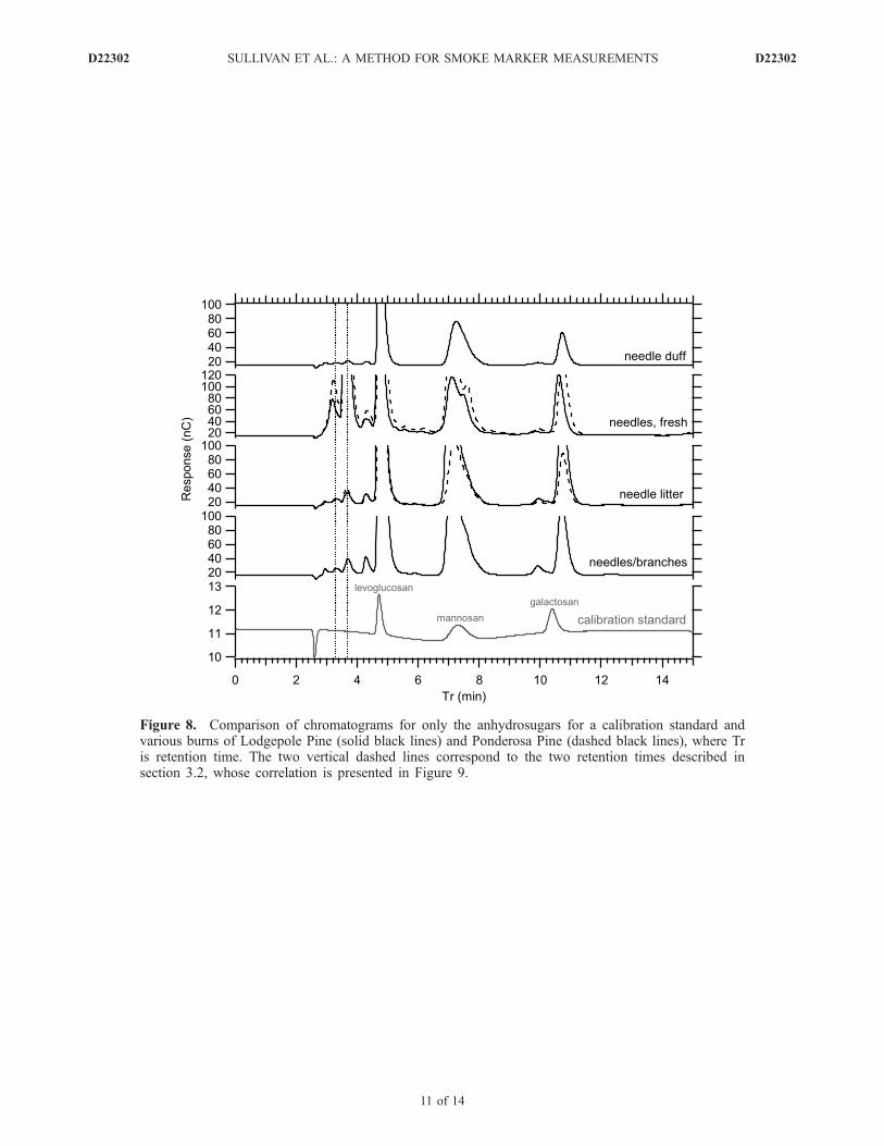
Figure 8. Comparison of chromatograms for only the anhydrosugars for a calibration standard andvarious burns of Lodgepole Pine (solid black lines) and Ponderosa Pine (dashed black lines), where Tris retention time. The two vertical dashed lines correspond to the two retention times described insection 3.2, whose correlation is presented in Figure 9.


11 of 14

D22302

potassium versus OC (not shown), which are correlated forbranches, straw, and grasses.

3.2. Potential Fingerprint Information

[41] It appears that information contained in the HPAEC-PAD chromatogram may provide insight about the type offuel component burned. Figure 8 shows a comparison oftypical chromatograms from a calibration standard and

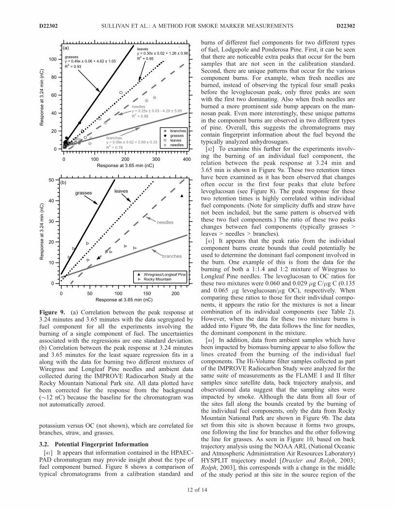
burns of different fuel components for two different typesof fuel, Lodgepole and Ponderosa Pine. First, it can be seenthat there are noticeable extra peaks that occur for the burnsamples that are not seen in the calibration standard.Second, there are unique patterns that occur for the variouscomponent burns. For example, when fresh needles areburned, instead of observing the typical four small peaksbefore the levoglucosan peak, only three peaks are seenwith the first two dominating. Also when fresh needles areburned a more prominent side bump appears on the man-nosan peak. Even more interestingly, these unique patternsin the component burns are observed in two different typesof pine. Overall, this suggests the chromatograms maycontain fingerprint information about the fuel beyond thetypically analyzed anhydrosugars.[42] To examine this further for the experiments involv-

ing the burning of an individual fuel component, therelation between the peak response at 3.24 min and3.65 min is shown in Figure 9a. These two retention timeshave been examined as it has been observed that changesoften occur in the first four peaks that elute beforelevoglucosan (see Figure 8). The peak response for thesetwo retention times is highly correlated within individualfuel components. (Note for simplicity duffs and straw havenot been included, but the same pattern is observed withthese two fuel components.) The ratio of these two peakschanges between fuel components (typically grasses >leaves > needles > branches).[43] It appears that the peak ratio from the individual

component burns create bounds that could potentially beused to determine the dominant fuel component involved inthe burn. One example of this is from the data for theburning of both a 1:1.4 and 1:2 mixture of Wiregrass toLongleaf Pine needles. The levoglucosan to OC ratios forthese two mixtures were 0.060 and 0.029 mg C/mg C (0.135and 0.065 mg levoglucosan/mg OC), respectively. Whencomparing these ratios to those for their individual compo-nents, it appears the ratio for the mixtures is not a linearcombination of its individual components (see Table 2).However, when the data for these two mixture burns isadded into Figure 9b, the data follows the line for needles,the dominant component in the mixture.[44] In addition, data from ambient samples which have

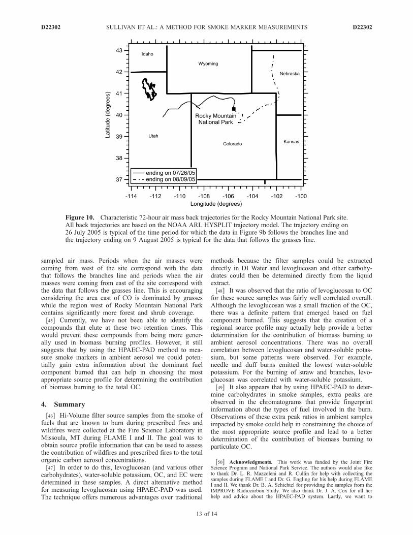
been impacted by biomass burning appear to also follow thelines created from the burning of the individual fuelcomponents. The Hi-Volume filter samples collected as partof the IMPROVE Radiocarbon Study were analyzed for thesame suite of measurements as the FLAME I and II filtersamples since satellite data, back trajectory analysis, andobservational data suggest that the sampling sites wereimpacted by smoke. Although the data from all four ofthe sites fall along the bounds created by the burning ofthe individual fuel components, only the data from RockyMountain National Park are shown in Figure 9b. The dataset from this site is shown because it forms two groups,one following the line for branches and the other followingthe line for grasses. As seen in Figure 10, based on backtrajectory analysis using the NOAA ARL (National Oceanicand Atmospheric Administration Air Resources Laboratory)HYSPLIT trajectory model [Draxler and Rolph, 2003;Rolph, 2003], this corresponds with a change in the middleof the study period at this site in the source region of the

Figure 9. (a) Correlation between the peak response at3.24 minutes and 3.65 minutes with the data segregated byfuel component for all the experiments involving theburning of a single component of fuel. The uncertaintiesassociated with the regressions are one standard deviation.(b) Correlation between the peak response at 3.24 minutesand 3.65 minutes for the least square regression fits in aalong with the data for burning two different mixtures ofWiregrass and Longleaf Pine needles and ambient datacollected during the IMPROVE Radiocarbon Study at theRocky Mountain National Park site. All data plotted havebeen corrected for the response from the background(�12 nC) because the baseline for the chromatogram wasnot automatically zeroed.


12 of 14

D22302

sampled air mass. Periods when the air masses werecoming from west of the site correspond with the datathat follows the branches line and periods when the airmasses were coming from east of the site correspond withthe data that follows the grasses line. This is encouragingconsidering the area east of CO is dominated by grasseswhile the region west of Rocky Mountain National Parkcontains significantly more forest and shrub coverage.[45] Currently, we have not been able to identify the

compounds that elute at these two retention times. Thiswould prevent these compounds from being more gener-ally used in biomass burning profiles. However, it stillsuggests that by using the HPAEC-PAD method to mea-sure smoke markers in ambient aerosol we could poten-tially gain extra information about the dominant fuelcomponent burned that can help in choosing the mostappropriate source profile for determining the contributionof biomass burning to the total OC.

4. Summary

[46] Hi-Volume filter source samples from the smoke offuels that are known to burn during prescribed fires andwildfires were collected at the Fire Science Laboratory inMissoula, MT during FLAME I and II. The goal was toobtain source profile information that can be used to assessthe contribution of wildfires and prescribed fires to the totalorganic carbon aerosol concentrations.[47] In order to do this, levoglucosan (and various other

carbohydrates), water-soluble potassium, OC, and EC weredetermined in these samples. A direct alternative methodfor measuring levoglucosan using HPAEC-PAD was used.The technique offers numerous advantages over traditional

methods because the filter samples could be extracteddirectly in DI Water and levoglucosan and other carbohy-drates could then be determined directly from the liquidextract.[48] It was observed that the ratio of levoglucosan to OC

for these source samples was fairly well correlated overall.Although the levoglucosan was a small fraction of the OC,there was a definite pattern that emerged based on fuelcomponent burned. This suggests that the creation of aregional source profile may actually help provide a betterdetermination for the contribution of biomass burning toambient aerosol concentrations. There was no overallcorrelation between levoglucosan and water-soluble potas-sium, but some patterns were observed. For example,needle and duff burns emitted the lowest water-solublepotassium. For the burning of straw and branches, levo-glucosan was correlated with water-soluble potassium.[49] It also appears that by using HPAEC-PAD to deter-

mine carbohydrates in smoke samples, extra peaks areobserved in the chromatograms that provide fingerprintinformation about the types of fuel involved in the burn.Observations of these extra peak ratios in ambient samplesimpacted by smoke could help in constraining the choice ofthe most appropriate source profile and lead to a betterdetermination of the contribution of biomass burning toparticulate OC.

[50] Acknowledgments. This work was funded by the Joint FireScience Program and National Park Service. The authors would also liketo thank Dr. L. R. Mazzoleni and R. Cullin for help with collecting thesamples during FLAME I and Dr. G. Engling for his help during FLAMEI and II. We thank Dr. B. A. Schichtel for providing the samples from theIMPROVE Radiocarbon Study. We also thank Dr. J. A. Cox for all herhelp and advice about the HPAEC-PAD system. Lastly, we want to

Figure 10. Characteristic 72-hour air mass back trajectories for the Rocky Mountain National Park site.All back trajectories are based on the NOAA ARL HYSPLIT trajectory model. The trajectory ending on26 July 2005 is typical of the time period for which the data in Figure 9b follows the branches line andthe trajectory ending on 9 August 2005 is typical for the data that follows the grasses line.


13 of 14

D22302

acknowledge M. Chandler, J. Chong, D. Davis, Dr. G. Engling, E. Garrell,Dr. G. Gonzalez, S. Grace, J. Hinkley, R. Jandt, R. Moore, S. Mucci,R. Olson, Dr. K. Outcalt, J. Reardon, Dr. K. Robertson, P. Spaine, andDr. D. Weise for providing the fuels used during FLAME I and II.

ReferencesAndreae, M. O. (1983), Soot carbon and excess fine potassium: Long-rangetransport of combustion-derived aerosols, Science, 220, 1148–1151.

Bauer, H., M. Claeys, R. Vermeylen, E. Schueller, G. Weinke, A. Berger,and H. Puxbaum (2008a), Arabitol and mannitol as tracers for the quan-tification of airborne fungal spores, Atmos. Environ., 42, 588–593.

Bauer, H., E. Schueller, G. Weinke, A. Berger, R. Hitzenberger, I. L. Marr,and H. Puxbaum (2008b), Significant contributions of fungal spores tothe organic carbon and to the aerosol mass balance of the urban atmo-spheric aerosol, Atmos. Environ., doi:10.1016/j.atmosenv.2008.03.019.

Baumann, K., F. Ift, J. Z. Zhao, and W. L. Chameides (2003), Discretemeasurements of reactive gases and fine particle mass and compositionduring the 1999 Atlanta Supersite Experiment, J. Geophys. Res.,108(D7), 8416, doi:10.1029/2001JD001210.

Birch, M. E., and R. A. Cary (1996), Elemental carbon-based method formonitoring occupational exposures to particulate diesel exhaust, AerosolSci. Technol., 25, 221–241.

Caseiro, A., I. L. Marr, M. Claeys, A. Kasper-Giebl, H. Puxbaum, andC. A. Pio (2007), Determination of saccharides in atmospheric aerosolusing anion-exchange high-performance liquid chromatography andpulse-amperometric detection, J. Chromatogr. A, 1171, 37–45.

Christian, T. J., B. Kleiss, R. J. Yokelson, R. Holzinger, P. J. Crutzen,W. M. Hao, T. Shirai, and D. R. Blake (2004), Comprehensive laboratorymeasurements of biomass-burning emissions: 2. First intercomparison ofopen-path FTIR, PTR-MS, and GC-MS/FID/ECD, J. Geophys. Res.,109, D02311, doi:10.1029/2003JD003874.

Draxler, R. R., and G. D. Rolph (2003), HYSPLIT (HYbrid Single-ParticleLagrangian Integrated Trajectory) Model access via NOAA ARLREADY Website (Available at http://www.arl.noaa.gov/ready/hysplit4.html), NOAA Air Resources Laboratory, Silver Spring, Md.

Eller, P. M., and M. E. Cassinelli (Eds.) (1996), NIOSH Manual of Analy-tical Methods, 4th Edition (1st Supplement), National Institute for Occu-pational Safety and Health, Cincinnati, Ohio.

Engling, G. (2006), Characterizing biomass combustion emission contribu-tions to ambient aerosol concentrations, Ph.D. thesis, Colorado StateUniversity, Colo.

Engling, G., C. M. Carrico, S. M. Kreidenweis, J. L. Collett Jr., D. E. Day,W. C. Malm, E. Lincoln, W. M. Hao, Y. Iinuma, and H. Herrmann(2006), Determination of levoglucosan in biomass combustion aerosolby high-performance anion-exchange chromatography with pulsed am-perometric detection, Atmos. Environ., 40, S299-311.

Fine, P. M., G. R. Cass, and B. R. T. Simoneit (2004), Chemical character-ization of fine particle emissions from the fireplace combustion of woodtypes grown in the Midwestern and Western United States, Environ. Eng.Sci., 21, 387–409.

Fraser, M. P., Z. W. Yue, and B. Buzcu (2003), Source appointment of fineparticulate matter in Houston, TX, using organic molecular markers,Atmos. Environ., 37, 2117–2123.

Gao, S., D. A. Hegg, P. V. Hobbs, T. W. Krirchstetter, B. I. Magi, andM. Sadilek (2003), Water-soluble organic components in aerosols asso-ciated with savanna fires in southern Africa: Identification, evolution, anddistribution, J. Geophys. Res., 108(D13), 8491, doi:10.1029/2002JD002324.

Gorin, C. A., J. L. Collett Jr., and P. Herckes (2006), Wood smoke con-tribution to winter aerosol in Fresno, CA, J. Air Waste Manage. Assoc.,56, 1584–1590.

Hays, M. D., C. D. Geron, K. J. Linna, N. D. Smith, and J. J. Schauer(2002), Speciation of gas-phase and fine particle emissions from burningof foliar fuels, Environ. Sci. Technol., 36, 2281–2295.

Herckes, P., G. Engling, S. M. Kreidenweis, and J. L. Collett Jr. (2006),Particle size distributions of organic aerosol constituents during the 2002Yosemite Aerosol Characterization Study, Environ. Sci. Technol., 40,4554–4562.

Hoch, G. (2007), Cell wall hemicelluloses as mobile carbon stores in non-reproductive plant tissues, Funct. Ecol., 21, 823–834.

Mazzoleni, L. R., B. Zielinska, and H. Moosmuller (2007), Emissions oflevoglucosan, methoxy phenols, and organic acids from prescribed burns,laboratory combustion of wildland fuels, and residential wood combus-tion, Environ. Sci. Technol., 41, 2115–2122.

Nolte, C. G., J. J. Schauer, G. R. Cass, and B. R. T. Simoneit (2001), Highlypolar organic compounds present in wood smoke and in the ambientatmosphere, Environ. Sci. Technol., 33, 3313–3316.

Puxbaum, H., A. Caseiro, A. Sanchez-Ochoa, A. Kasper-Giebl, M. Claeys,A. Gelencser, M. Legrand, S. Preunkert, and C. Pio (2007), Levoglucosanlevels at background sites in Europe for assessing the impact of biomasscombustion on the European aerosol background, J. Geophys. Res., 112,D23S05, doi:10.1029/2006JD008114.

Rinehart, L. R., E. M. Fujita, J. C. Chow, K. Magliano, and B. Zielinska(2006), Spatial distribution of PM2.5 associated organic compounds incentral California, Atmos. Environ., 40, 290–303.

Rogge, W. F., L. M. Hildemann, M. A. Mazurek, G. R. Cass, and B. R. T.Simoneit (1998), Sources of fine organic aerosol. 9. Pine, oak, and syn-thetic log combustion in residential fireplaces, Environ. Sci. Technol., 32,13–22.

Rolph, G. D. (2003), Real-time Environmental Applications and DisplaysYstem (READY) Website (Available at http://www.arl.noaa.gov/ready/hysplit4.html), NOAA Air Resources Laboratory, Silver Spring, Md.

Schauer, J. J., and G. R. Cass (2000), Source apportionment of wintertimegas-phase and particle-phase air pollutants using organic compounds astracers, Environ. Sci. Technol., 34, 1821–1832.

Schauer, J. J., W. F. Rogge, L. M. Hildemann, M. A. Mazurek, andG. R. Cass (1996), Source apportionment of airborne particulate matterusing organic compounds as tracers, Atmos. Environ., 30, 3837–3855.

Schauer, J. J., M. J. Kleeman, G. R. Cass, and B. R. T. Simoneit (2001),Measurement of emissions from air pollution sources. 3. C1–C29 organiccompounds from fireplace combustion of wood, Environ. Sci. Technol.,35, 1716–1728.

Schichtel, B. A., W. C. Malm, G. Bench, S. Fallon, C. E. McDade,J. C. Chow, and J. G. Watson (2008), Fossil and contemporary fineparticulate carbon fractions at 12 rural and urban sites in the UnitedStates, J. Geophys. Res., 113, D02311, doi:10.1029/2007JD008605.

Simoneit, B. R. T., J. J. Schauer, C. G. Nolte, D. R. Oros, V. O. Elias,M. P. Fraser, W. F. Rogge, and G. R. Cass (1999), Levoglucosan, atracer for cellulose in biomass burning and atmospheric particles,Atmos. Environ., 33, 173–182.

Simpson, C. D., R. L. Dill, B. S. Katz, and D. A. Kalman (2004), Deter-mination of levoglucosan in atmospheric fine particulate matter, J. AirWaste Manage. Assoc., 54, 689–694.

Ward, D. E., and L. F. Radke (1993), Emission measurements from vegeta-tion fires: a comparative evaluation of methods and results, in Fire in theEnvironment: The Ecological, Atmospheric, and Climatic Importance ofVegetation Fires, edited by P. J. Crutzen and J. G. Goldammer, pp. 53–76, Wiley, Chichester, U.K.

Westerling, A. L., H. G. Hidalgo, D. R. Cayan, and T. W. Swetnam (2006),Warming and earlier spring increase Western U. S. forest wildfire activity,Science, 313, 940–943.

Zdrahal, Z., J. Oliveira, R. Vermeylen, M. Claeys, and W. Maenhaut (2002),Improved method for quantifying levoglucosan and related monosacchar-ide anhydrides in atmospheric aerosols and application to samples fromurban and tropical locations, Environ. Sci. Technol., 36, 747–753.

��J. L. Collett Jr., A. S. Holden, S. M. Kreidenweis, G. R. McMeeking,

L. A. Patterson, and A. P. Sullivan, Department of Atmospheric Science,Colorado State University, 1371 Campus Delivery, Fort Collins, CO80523, USA. ([email protected])W. M. Hao and C. E. Wold, USDA Forest Service, Fire Sciences

Laboratory, RWU 4404, 5775 West Highway 10, Missoula, MT 59808,USA.W. C. Malm, National Park Service/CIRA, Colorado State University,

1371 Campus Delivery, Fort Collins, CO 80523, USA.


14 of 14

D22302

Documents

A method for smoke marker measurements and its potential ... · of branches > straw > needles > leaves. ... populated areas, residential wood combustion, another form of biomass burning,