Embed Size (px)
Citation preview

A Method for Optical Measurement of Urea in Effluent Hemodialysate
by
Rebecca Kupcinskas
A Dissertation
Submitted to the faculty
of the
WORCESTER POLYTECHNIC INSTITUTE
in partial fulfillment of the requirements for the
Degree of Doctor of Philosophy
in
Biomedical Engineering
May 10, 2000
APPROVED:
Professor Robert A. Peura, Major Advisor
Professor Stevan Kun, Co-Advisor
Professor Len Polizzotto, Co-Advisor
Hannu Harjunmaa, Ph.D., Co-Advisor
Professor Ross D. Shonat, Co-Advisor
Professor Fred J. Looft, Co-Advisor Professor Christopher Sotak, Co-Advisor

ii
ABSTRACT
The addition of urea clearance monitoring to the care regimen of renal failure patients provides a dramatic decrease in complications due to improper or inadequate dialysis. Present methods of monitoring urea clearance are computationally complex and expensive to perform, resulting in poor rates of clinical acceptance of this measurement. Dialysate-side urea levels have been shown to relate to traditional measures of dialysis adequacy without the need for complex calculations. The requirements for photometric reagents or electrodes make determination of the urea level expensive and time consuming. This research is focused on the development of an optical measurement system to determine the sample urea level without the need for reagents. An algorithm was developed to predict the urea concentration of the sample from a set of optical transmission parameters recorded from the sample using a specially developed instrument. This instrument records the difference in sample transmission at two different wavelengths. Energy at the first wavelength is absorbed by urea, and the second wavelength is selected such that the matrix of the sample absorbs energy at both wavelengths equally. This effectively nulls out the absorbance of the background matrix, significantly improving the urea detection sensitivity. The algorithm was developed from an analysis of the instrument data and factors causing variations in the data. Calibration, bench study, and clinical protocols were designed, and performed using these protocols. Using a partial least squares approach, the algorithm was fit to a set of training data. The resulting algorithm was used to predict the urea content of patient hemodialysis samples. Compared to a reference standard (Beckman CX7, standard error <1 mg/dl), the standard error of prediction for this algorithm was 0.47 mg/dl (N = 34 patients). The algorithm was able to predict dialysate urea at clinically relevant levels in samples collected from hemodialysis patients. Qualitative relationships were developed between the sample urea level and the data recorded from the sample. This system has the potential to provide a method that clinicians can use to efficiently and effectively monitor urea removal over the course of a dialysis session.

iii
ACKNOWLEDGEMENTS I’d like to thank: My dad, mom, and Rachel for all of their moral support, and encouragement. Extra special thanks to dad for his help and countless hours in the machine shop. Dr. Robert Black and the nursing staff at the Worcester Medical Center for providing access to patients and information. Dr. Tom Ukena for analyzing the patient samples. My advisors – Dr. Peura, Dr. Polizzotto, Dr. Kun , Dr. Harjunmaa, Dr. Looft, Dr. Shonat, and Dr. Sotak for their professional and personal advice. Jamie for his friendship, advice, expertise, and company during long lab hours. Kim for her long distance advice. Leslie for her short distance advice. Chris for helping me remember where I left my sense of humor. Bryant for helping me remember where I left my sanity, and other things too numerous to mention.

iv
TABLE OF CONTENTS Chapter 1 INTRODUCTION – PROBLEM IDENTIFICATION .......................................... 1
1.1 Chronic Kidney Failure ................................................................................................................. 2 1.2 Acute Kidney Failure ..................................................................................................................... 2 1.3 Monitoring of Dialysis Efficiency .................................................................................................. 3 1.4 Summary ......................................................................................................................................... 3
2 THE SPECIFIC AIMS OF THE RESEARCH....................................................... 4 2.1 Project Statement ........................................................................................................................... 4 2.2 General System Requirements ...................................................................................................... 5
3 HYPOTHESES AND RESEARCH METHODS .................................................... 7 3.1 Hypotheses....................................................................................................................................... 7 3.2 Research Methods .......................................................................................................................... 7
4 BACKGROUND ...................................................................................................... 13 4.1 Kidney Function and Failure....................................................................................................... 13 4.2 Dialysis........................................................................................................................................... 19 4.3 Dialysate-Side vs. Blood-Side Measurements: A history of dialysis adequacy monitoring.... 33 4.4 Comparison with Presently Available Technology.................................................................... 35 4.5 Classical Absorption Spectrometry – The Beer-Lambert Law ................................................ 36 4.6 The Optical Bridge ....................................................................................................................... 37 4.7 The Near-IR Absorbance Characteristics of Urea and Water ................................................. 44 4.8 Analysis of Potential Interfering Substances.............................................................................. 47 4.9 Multiple Linear Regression ......................................................................................................... 52 4.10 Summary of Background Information ................................................................................. 54
5 DIALYSIS EFFICIENCY MONITORING SYSTEM DESIGN OVERVIEW 55 5.1 Design Overview ........................................................................................................................... 55 5.2 Description of Measurement Principles...................................................................................... 57 5.3 Measurement Procedure .............................................................................................................. 59 5.4 Measurement Implementation .................................................................................................... 61 5.5 Summary ....................................................................................................................................... 66
6 DESCRIPTION OF TESTING METHODOLOGY ............................................ 67 6.1 Baseline Studies ............................................................................................................................ 67 6.2 Urea Studies .................................................................................................................................. 68 6.3 Hemodialysis Patient Studies....................................................................................................... 70
7 ALGORITHMS FOR MONITORING DIALYSIS PERFORMANCE ............. 71 7.1 Linear Model with Correction Parameters ................................................................................ 71 7.2 Multiple Linear Regression Approach ....................................................................................... 76 7.3 MLR fitting concerns ................................................................................................................... 77 7.4 Choosing the Model Factors – The Evolution of the MLR Algorithm..................................... 79 7.5 Dialysis Efficiency Monitoring Algorithm.................................................................................. 83
8 EXPERIMENTAL RESULTS................................................................................ 85 8.1 Summary of Experiments ............................................................................................................ 85 8.2 Results of Proof of Principle Studies........................................................................................... 86 8.3 Baseline (no urea) studies............................................................................................................. 87 8.4 Results of the Urea Level Estimation Studies: Urea in Water Studies .................................... 97 8.5 Results of the Urea Level Estimation Studies: Hemodialysis Patient Studies ....................... 104 8.6 Results of Phantom Model Testing ........................................................................................... 109 8.7 Medical Interpretation of Estimated Urea Level Results and Projected Use for Dialysis Efficiency Monitoring ...................................................................................................................... 110

v
9 DISCUSSION ......................................................................................................... 111 9.1 Urea Monitoring System Instrument Design ........................................................................... 111 9.2 Urea Monitoring Algorithm Design .......................................................................................... 112 9.3 Proof of Principle Studies .......................................................................................................... 112 9.4 Hemodialysis Patient Testing..................................................................................................... 114 9.5 Significance of Results................................................................................................................ 115 9.6 Dialysis Monitoring System Testing Results ............................................................................ 116
10 CONCLUSION.................................................................................................. 117 11 FUTURE WORK .............................................................................................. 120 12 DISCLAIMER................................................................................................... 121 13 REFERENCES.................................................................................................. 122
vi
LIST OF FIGURES Figure 3.2.1: Schematic diagram of a differential spectrophotometer. .......................................................... 9 Figure 3.2.2: Schematic diagram of an optical bridge instrument ................................................................. 9 Figure 3.2.3: Flowchart of the research approach....................................................................................... 12 Figure 4.1.1: Gross anatomy of the normal human kidneys. ........................................................................ 14 Figure 4.1.2: Highly magnified diagram of a single nephron ...................................................................... 15 Figure 4.2.1: Diagram of Hemodialysis Set-up ............................................................................................ 20 Figure 4.2.2: Exchange of toxins occurs between various fluid compartments during dialysis as a function of concentration and potential gradients ...................................................................................................... 23 Figure 4.2.3: The chemical structure of urea ............................................................................................... 24 Figure 4.2.4: NH3 is converted to carbamoyl phosphate in the first step of the Kreb's cycle....................... 31 Figure 4.2.5: The TCA cycle links together with the urea cycle to form the Kreb’s bicycle......................... 31 Figure 4.2.6: The urea cycle takes place in the cytosol and mitochondria of the liver cell.......................... 32 Figure 4.6.1: The Reference and Principal wavelengths are selected according to the criteria stated in §4.4.1. ........................................................................................................................................................... 39 Figure 4.6.2: The Optical Bridge input signal during three phases of the measurement. ............................ 41 Figure 4.6.3: Light intensity at the entrance and exit of the sample is represented for each wavelength phase by the length of the arrow................................................................................................................... 42 Figure 4.7.1: Absorbance spectrum for water in the mid-IR. ....................................................................... 45 Figure 4.7.2: Absorbance spectrum for water in the Near-IR. ..................................................................... 46 Figure 4.7.3: Reflectance spectrum for dry urea in the Near-IR. ................................................................. 47 Figure 4.8.1: This bar graph shows the unit absorbance (per mg/dl) of many potential interferents in the spent dialysate fluid. ..................................................................................................................................... 50 Figure 4.8.2: This graph shows the logarithm of the sensitivity factor of each compound. ......................... 51 Figure 4.8.3: This graph shows the location of harmonics bands of potential interferents.......................... 52 Figure 5.1.1: Signal block diagram of the system ........................................................................................ 56 Figure 5.3.1: Simulated data showing that the residual AC signal in each of the balancing positions (intensity and wavelength) is extrapolated out to an induced error in the measurement position................ 61 Figure 5.4.1: Urea monitoring system software block diagram. .................................................................. 62 Figure 5.4.2: The measurement fluid is contained in a Teflon bag .............................................................. 63 Figure 5.4.3: The measurement cuvette has two chambers, each of which contains a teflon bag................ 63 Figure 5.4.4: Diagram of fluid control unit.................................................................................................. 64 Figure 5.4.5: Dimensions of the measurement head of the NIV Prototype................................................... 65 Figure 5.4.6: Transmission of two layers of 0.01" silicon membrane. ......................................................... 65 Figure 5.4.7: Assembly drawing and picture of the measurement cuvette. .................................................. 66 Figure 7.1.1: The residual AC signal in the 00 and 0 position is projected into the 1 position.................... 73 Figure 7.1.2: The residual AC signal after balancing must be partitioned into a shift term and a slope term...................................................................................................................................................................... 74 Figure 8.2.1: Estimated vs. Actual Urea for the dissertation prototype. ...................................................... 86 Figure 8.2.2: Estimated vs. Actual Urea, dissertation prototype.................................................................. 87 Figure 8.3.1: Offset is strongly related to (left) sample temperature ........................................................... 90 Figure 8.3.2: AC00 and AC0 are strongly correlated .................................................................................. 91 Figure 8.3.3: Sample thickness is strongly related to DC values at the sample detector ............................. 91 Figure 8.3.4: Plot of the correlation matrix for a baseline study ................................................................. 89 Figure 8.3.5: The light transmission through the sample is an increasing function of temperature ............ 93 Figure 8.3.6: The sensitivity of the AD to increasing sample temperature is an order of magnitude lower than that of the SD and shows a dependence on wavelength........................................................................ 94 Figure 8.3.7: The R_INT voltage also increases linearly with sample temperature..................................... 94 Figure 8.3.8: The offset voltage that was required to balance the bridge decreased as a function of sample temperature................................................................................................................................................... 95 Figure 8.3.9: Response of the signal to temperature variations ................................................................... 96 Figure 8.3.10: Variation of the AC signal with sample temperature at three wavelengths .......................... 97 Figure 8.4.1: Urea Estimation Calibration curve for algorithm 1 ............................................................... 98

vii
Figure 8.4.2: These 40 AC measurements were recorded from the same sample. ....................................... 98 Figure 8.4.3: These two figures demonstrate the variation of AC1 with sample temperature...................... 99 Figure 8.4.4: These four graphs show how the drift in AC1 is related to drift in the offset and reference wavelength .................................................................................................................................................. 100 Figure 8.4.5: Variation of AC1 with sample thickness ............................................................................... 101 Figure 8.4.6: AC1 and K, the transparency ratio, follow inverse trends to each other.............................. 101 Figure 8.4.7: Calibration curve for urea in water studies: estimated urea vs. actual urea........................ 104 Figure 8.5.1: Urea Estimation Calibration curve for algorithm 1 ............................................................. 105 Figure 8.5.2: Calibration curve of measured urea vs. estimated urea ....................................................... 107 Figure 8.5.3: Scatter diagram for the hemodialysis patient study.............................................................. 108

viii
LIST OF TABLES Table 3.2.1: Experimental Design Matrix..................................................................................................... 10 Table 4.1.1: Partial list of substances that may be responsible for symptoms of uremia ............................. 27 Table 4.2.2: Factors influencing solute removal during dialysis [68]. ........................................................ 29 Table 4.4.1: Cost comparison of proposed system vs. existing technology. ................................................. 35 Table 4.8.1: List of potential interferents in spent dialysate......................................................................... 48 Table 4.9.1: Analysis of Variation (ANOVA) Table...................................................................................... 53 Table 5.2.1: List of system parameters and their symbols. ........................................................................... 58 Table 7.4.1: List and description of data items obtained from each measurement....................................... 79 Table 7.4.2: Weighting coefficients for the MLR algorithm.......................................................................... 83 Table 8.1.1 : Overview of the performed experiments and measurements. .................................................. 86 Table 8.3.1: Groupings of variables showing possible dependencies........................................................... 89 Table 8.3.2: Rate of change of various signals with temperature................................................................. 92 Table 8.3.3: ANOVA table for the temperature study. .................................................................................. 92 Table 8.3.4: The rate of change of AC vs. temperature depends on wavelength. ......................................... 96 Table 8.4.1: MLS Result Table: urea in water study. ................................................................................. 103 Table 8.4.2: Results of Urea Estimation Study ........................................................................................... 103 Table 8.5.1: MLS Result Table: Hemodialysis sample study. ..................................................................... 106 Table 8.5.2: Results of the MLS urea estimation algorithm: hemodialysis study ....................................... 108 Table 8.5.3: ANOVA table comparing the urea results obtained with the MLS algorithm to the clinical standard instrument. ................................................................................................................................... 109

1
1 INTRODUCTION – PROBLEM IDENTIFICATION Kidney dialysis is a lifesaving procedure that is used to sustain the health of patients who have experienced renal failure. Patients require dialysis for a variety of reasons. The most common reason is chronic kidney failure due to scarring or necrosis of kidney tissue as a complication of diabetes. A second cause of chronic kidney failure is uncontrolled high blood pressure. Other reasons for requiring dialysis treatment include acute cessation of kidney function caused by poisoning or drug overdose. Certain diseases, including urinary tract infection, polycystic kidney disease, and acute glomerulonephritism may temporarily shut down kidney function sufficiently to require dialysis. In the year 2000, there are approximately 250,000 patients undergoing dialysis treatment in the United States [1]. While dialysis is a simple process, many of its effects on the body are not fully understood. This lack of knowledge translates to questions about whether or not the therapy patients receive is being delivered in an optimal fashion. Articles appear in the literature relating to methods of quantifying and optimizing dialysis efficiency [2-48]. These methods generally propose mathematical models relating the results of blood tests and parameters of the dialysis machine to the expected outcome, namely a measure of the patient’s total toxin clearance at the end of the session. These methods are not widely used, ostensibly because of their computational complexity. Most practicing physicians choose to ignore these models, relying instead on empirical calculations of therapy requirements and subjective evaluations of the patient’s progress. Since many of the effects of dialysis on the body are subtle, and insufficiently understood at the present time, quantifying the effectiveness of dialysis is a significant problem for the clinical practitioner. A few instruments have been developed to calculate certain dialysis parameters, but they generally require regular maintenance and significant additional work from the caregivers [2-11]. In recent years, the technology used in dialysis machines has changed, reducing the amount of time that patients must spend in dialysis. At the same time, the mortality rate of these patients has increased significantly [12-16, 49]. The mortality data seems to suggest that newer dialysis methods are failing to adequately cleanse the patient’s blood of toxins. To complicate the problem, the effects of inadequate dialysis are not immediately apparent. It may take weeks, months, or even years for the effects of sub-optimal therapy to appear. For this reason, it seems imperative that the patient’s progress be monitored during every dialysis session, and that an automatic method that can more accurately describe the effects of the dialysis process on the patient is needed to ensure that these patients receive the best possible care. This method must be easy to use, and provide information that a physician would consider useful if it is to gain clinical acceptance.
2
1.1 Chronic Kidney Failure
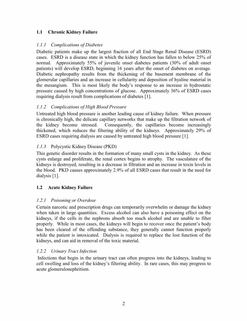
1.1.1 Complications of Diabetes Diabetic patients make up the largest fraction of all End Stage Renal Disease (ESRD) cases. ESRD is a disease state in which the kidney function has fallen to below 25% of normal. Approximately 55% of juvenile onset diabetes patients (30% of adult onset patients) will develop ESRD, beginning 16 years after the onset of diabetes on average. Diabetic nephropathy results from the thickening of the basement membrane of the glomerular capillaries and an increase in cellularity and deposition of hyaline material in the mesangium. This is most likely the body’s response to an increase in hydrostatic pressure caused by high concentrations of glucose. Approximately 36% of ESRD cases requiring dialysis result from complications of diabetes [1].
1.1.2 Complications of High Blood Pressure Untreated high blood pressure is another leading cause of kidney failure. When pressure is chronically high, the delicate capillary networks that make up the filtration network of the kidney become stressed. Consequently, the capillaries become increasingly thickened, which reduces the filtering ability of the kidneys. Approximately 29% of ESRD cases requiring dialysis are caused by untreated high blood pressure [1].
1.1.3 Polycystic Kidney Disease (PKD) This genetic disorder results in the formation of many small cysts in the kidney. As these cysts enlarge and proliferate, the renal cortex begins to atrophy. The vasculature of the kidneys is destroyed, resulting in a decrease in filtration and an increase in toxin levels in the blood. PKD causes approximately 2.9% of all ESRD cases that result in the need for dialysis [1].
1.2 Acute Kidney Failure
1.2.1 Poisoning or Overdose Certain narcotic and prescription drugs can temporarily overwhelm or damage the kidney when taken in large quantities. Excess alcohol can also have a poisoning effect on the kidneys, if the cells in the nephrons absorb too much alcohol and are unable to filter properly. While in most cases, the kidneys will begin to recover once the patient’s body has been cleared of the offending substance, they generally cannot function properly while the patient is intoxicated. Dialysis is required to replace the lost function of the kidneys, and can aid in removal of the toxic material.
1.2.2 Urinary Tract Infection Infections that begin in the urinary tract can often progress into the kidneys, leading to cell swelling and loss of the kidney’s filtering ability. In rare cases, this may progress to acute glomerulonephritism.

3
1.2.3 Acute Glomerulonephritism This disease is often caused by a streptococcal infection. The infection causes a rapid swelling of the kidney and a corresponding loss of function. The tissues of the kidney become choked with leukocytes, and are unable to perform their filtering function. Dialysis is required to compensate for the kidney function while the infection is treated. Once the infection is clear, the kidneys are generally able to resume normal function. Approximately 11% of the patients who require dialysis have experienced glomerulonephritis [1].
1.3 Monitoring of Dialysis Efficiency There are many factors that can be monitored during dialysis with the goal of quantifying dialysis effectiveness and efficiency. These factors include, but are not limited to: toxin removal rate, protein catabolic rate, estimation of residual kidney function, and kinetics of fluid compartment shifts. All of this information can be useful to the physician when deciding how well the prescribed treatment is helping the dialysis patient. In monitoring dialysis, it is necessary to solve one problem – how to quantify dialysis efficiency in a non-invasive, automatic, accurate, and continuous manner. While many techniques exist to quantify some of these requirements, none exists which satisfies them all. A general solution to this problem has not yet been developed. Development of a technique for monitoring dialysis efficiency would be a tremendous value to both clinical practitioners and dialysis patients. The complications from inadequate dialysis could be reduced or prevented altogether. In addition, such a technique could reduce the incidence of over-dialysis, which can be detrimental to the patient both mentally and physically. In the case of chronic renal insufficiency, keeping toxin levels low could reduce further system failure. In acute cases, monitoring could speed recovery time by ensuring that toxins are removed as quickly and completely as possible.
1.4 Summary The lack of a method for assessing dialysis efficiency that is simple to use, non-invasive, continuous, accurate, and efficient, presents an important clinical problem. The problem is original, and its solution requires application of the principles of scientific analysis and synthesis to develop new measurement systems. However, major improvements can and must be made evident compared to other techniques in order for the new technique to find clinical acceptance.

4
2 THE SPECIFIC AIMS OF THE RESEARCH
2.1 Project Statement The long-term goal of this research is to develop a clinical instrument that can be used to quantify the efficiency and effectiveness of a dialysis session in a non-invasive, automatic, and accurate manner for any patient undergoing dialysis. To address this goal, we will develop a prototype instrumentation system that is able to measure the amount of urea that is being removed by dialysis from a patient with ESRD. Based on the use of this instrument, an algorithm will be developed that can produce an estimate of the urea content of an aqueous sample based on data obtained from this system. We do not intend to directly interface this system to a dialysis machine during this phase of research. Rather, the development of this demonstration system represents a major advance in the field of renal failure therapy by providing a ‘closed loop’ approach to determining adequacy of therapy and eliminating the guesswork involved in current methods. The automatic, low maintenance nature of this system provides a high potential for clinical acceptance of the technology and the possibility of saving lives by reducing complications from poor dialysis. In order to achieve the goals stated above, the specific aims that must be completed are to; 1) Develop and build an instrument that is based on the principles of an Optical Bridge –
an instrument that measures the difference in energy absorbance between two wavelengths of light. The wavelengths of light are selected such that urea preferentially absorbs energy at the first, but not at the other. a) Design and build a completely automatic system that can deliver light at
appropriate wavelengths and measure the light transmittance through a fluid sample, transferring the results to an IBM compatible personal computer. The system should satisfy normal safety requirements for a medical instrument.
b) Develop software for controlling the delivered light intensity and wavelength, controlling the operation of the prototype hardware, and collecting, storing, analyzing, and displaying the urea level measurements.
2) Perform preliminary studies with this new system using samples of fluid spiked with
urea and water. Urea studies will also be done on an existing prototype instrument originally developed for non-invasive glucose monitoring, and compared to the results obtained with the new system.
3) Using the data obtained in Specific Aim 2, develop an algorithm for correlating the
measurements with the urea concentration; a) Develop a mathematical model relating the instrument output to urea
concentration.

5
b) Develop a mathematical model based on experimental data that describes how the instrument reading can be affected by variations in the environment (including temperature) and other major interferences.
c) Determine which of these variations may prove significant, and propose and develop methods to compensate for them.
d) Develop an algorithm for urea level monitoring.
4) Perform preliminary clinical studies with the system using the algorithm developed in Specific Aim 3. a) Perform a pilot study using samples of spent dialysate from human subjects. b) Compare the predicted urea concentration of these samples to a clinically standard
reference method. c) Compare the predicted vs. measured sample urea content statistically. We
propose that the difference in mean should be zero to a significance level of 0.01. Additionally, find a 95% confidence interval for the true difference in sample mean. Find a 95% confidence interval for the variance ratio between the two measurements.
2.2 General System Requirements There is no general agreement as to what the exact requirements and specifications of a dialysis monitoring system should be. In order to ensure that this instrument provides useful and accurate estimates of dialysis accuracy, performance specifications must be developed, and it must be shown that the instrument meets these specifications. First, we need to know the expected ranges of the dialysate urea concentration, and to have an idea of how accurately we need to be able to determine its value. We then need to know how often we need to measure this parameter in order to obtain a true representation of its time dependence. We must also know how long the instrument must be stable for: In other words, for how long must a calibration be valid? Finally, it is necessary to know how the instrument responds in the presence of other interfering inputs, or how specific its response is to the dialysate urea level in the presence of other analytes. We will now discuss the requirements that this instrument must meet:
• = Range – Dialysate urea levels generally fall between 6 and 180 mg/dl [6]. • = Accuracy/Precision – Standard clinical analysis tools provide an accuracy of ±1-2
mg/dl for urea measurements. Clinical practitioners indicate that an accuracy of 10 mg/dl or better is acceptable [50].
• = Frequency of measurement – The main advantage of an automated technique is that it provides information on the patient’s urea level as a function of time, rather than an indirect interpolation from start to finish Blood Urea Nitrogen (BUN) levels. Most researchers agree that urea follows a double exponential removal profile in the body that is mirrored in the dialysate. The measurement sampling frequency must be high enough to capture this profile. The stream must be sampled at a rate fast enough to capture the time constant for each pool. The results can then be plotted logarithmically and the time constant obtained from this graph. In general, results should be taken for this measurement every fifteen to thirty minutes [6]. A second parameter that may be useful to the clinician is the

6
total amount of urea removed during the session. This can be calculated by measuring the area under the curve of urea concentration versus time. This measurement can be done every ten minutes or so.
• = Stability – The measurement should be accurate without need for recalibration over a weekly cycle. Most patients are dialyzed three times per week, and it is necessary to compare the results between sessions.
• = Specificity – There are a myriad of other substances in the dialysate that can potentially interfere with the urea measurement.
Finally, from an economic viewpoint, our approach has the potential to solve many of the problems with the existing technology in that the cost per test would be far lower due the lack of need for reagents and electrodes. The final cost of the system is projected to be around $3000-$5000, compared to $1000 for existing technology (such as Baxter Healthcare’s Biostat 1000). (Future research involving the use of tunable diode lasers as light sources could bring the cost of this device into the $300-$500 range). The extra cost of the instrument could be easily offset by considering the cost of disposables items that are required by existing devices. Assuming that one machine can support 10 patients, who are each dialyzed three times per week, 52 weeks per year, at $3.50 per test, three tests per session, the disposable cost for existing technology per machine per year is approximately $16,380. This figure only includes electrodes and reagents, no extra supplies such as tubing, syringes, or extra laboratory tests.

7
3 HYPOTHESES AND RESEARCH METHODS The primary goal of this research is to develop a method to optically measure the concentration of urea in effluent dialysate without the need for reagents. To date, no one has reported success in using optical techniques to measure urea in aqueous solutions.
3.1 Hypotheses The central hypotheses of this research are: 1) A method based on differences in transmission of near infrared light energy can be employed in the development of an instrument that could provide information related to biologically relevant levels of urea in a strongly absorbing background matrix composed primarily of water. This urea information can be extracted amidst interferences such as temperature variations and the presence of other analytes (proteins and amino acids, sugars, electrolytes, metabolic wastes, etc.). 2) It is possible to develop an algorithm using the information obtained from the instrument to quantitatively and qualitatively estimate the amount of urea in an effluent stream of dialysate, and from this to evaluate the effectiveness of the dialysis session. 3) A list of major factors affecting the system response can be developed. While it is possible to obtain a first-guess list of factors from the non-invasive glucose measurement research, it is unlikely that the same set of factors will fit the urea measurement. We propose to determine how changes in temperature and dialysate composition affect the measurements, develop a list of parameters to represent these effects, and then perform a statistical analysis to determine the significance of each parameter to the overall measurements. 4) A mathematical model and corresponding algorithm can be developed which approximates the expected response of the system to changing urea concentration in the presence of interferences (such as other metabolic analytes) and modifying factors (such as temperature changes). This model will be based on a mathematical analysis of experimental data. A linear model based on a Multiple Linear Regression (MLR) or Partial Least Squares (PLS) approach can be used to correlate the output of the system with the expected urea concentration in dialysate. This will involve the development of an algorithm to relate system data to urea concentration.
3.2 Research Methods A method based on differences in transmission of near-IR light energy was chosen to solve the main research problem (see Chapter 1) for the following reasons: • = Optical measurements are well suited for this type of measurement. Other
possibilities in terms of measuring substances levels in a fluid stream such as

8
ultrasound and electromagnetic flowmeters are unable to distinguish between analytes, which prevents their use for this application. Optical measurements can be made specific to urea by selecting appropriate analysis wavelengths.
• = This is a non-invasive measurement method and is therefore not harmful to the patient. The measurement can be done on the spent (effluent) dialysis stream, which is normally sent to a waste drain, and therefore does not interfere with the normal operation of the dialysis machine or other clinical devices. The measurement is also automatic and easy to set up. In addition, spent dialysate is not considered a biohazard, so no special handling protocols are required.
• = Our preliminary results show that such wavelengths exist at which it is possible to measure urea with this “Optical Bridge” method [51]. Harjunmaa [52-56] has proposed that this method can be used in vivo for accurately measuring glucose levels in diabetic patients. Preliminary testing results with that application have been promising. Urea levels and glucose levels are of the same order of magnitude.
• = No one has reported results on using this method for measuring urea levels. The application of this method for monitoring urea levels, and consequently dialysis efficiency is a novel approach, and will improve upon existing knowledge in the field of dialysis patient monitoring.
In order to develop a system that is capable of monitoring urea, it is first necessary to establish a relationship between the signal and the dialysate urea concentration. The overall relationship is expected to be a linear function, since equations relating the Optical Bridge signal to concentration have been developed previously and hypothesized to show a linear relationship [52]. In order to improve the algorithm, it may be necessary to include other factors and correction parameters into the overall system equation. These parameters are also expected to relate to the original model in a linear fashion. It will be necessary to determine how each of the factors found in testing the third main hypothesis correlate to the overall signal in order to determine how an appropriate correction can be made. Our goal is to develop an instrument that is capable of monitoring the dialysate-side urea concentration without the need for electrodes or reagents. This has not been achieved by others. (See §4.4 for a discussion of existing technology for dialysate urea monitoring.) A specially developed algorithm should relate optical transmission parameters to the urea content of the sample. The proposed instrument directs a beam of light through a sample consisting of both spent and clean dialysate. The light beam alternates between two wavelengths. The first wavelength is one at which urea preferentially absorbs energy. The second wavelength is selected at measurement time so that the transmission through the clean dialysate is the same as at the first wavelength. The urea level of the sample is then proportional to the difference in sample transmission between the two wavelengths. Because the measurement is in a differential rather than an absolute mode, a large gain can be applied to the signal, which overcomes dynamic range limitations of conventional optical measurements. At first glance, this system may seem unnecessarily complicated. It would be simpler to measure the difference in transmission between the clean and spent dialysate at some

9
wavelength that is sensitive to urea, and then amplify this resulting signal. An instrument based on this method is shown in Figure 3.2.1. This instrument requires two optical detectors, one for the clean dialysate and one for the spent dialysate. The outputs of the two detectors are then fed into a differential amplifier.
Figure 3.2.1: Schematic diagram of a differential spectrophotometer.
In contrast, our design is shown in Figure 3.2.2. Here, the two samples are juxtaposed and only one detector is required. The light beam entering the samples consists of light energy two different wavelengths alternating at approximately 1 kHz. The signal coming from the detector is then AC coupled into a phase sensitive detector, and is then amplified. The AC coupling is necessary to eliminate DC drift that occurs in the detector and associated electronics with temperature changes and over time.
Figure 3.2.2: Schematic diagram of an optical bridge instrument
The main problem with the first instrument is the existence of two light and signal paths. To date, no one has reported success using this method. No matter how closely matched the detectors are, if they are at different temperatures, they will experience drift at different rates. Since the detectors are physically separated, it is not possible to keep them at exactly the same temperature. There is no mechanism with this circuit to cancel this drift. Our approach is to adopt the “Optical Bridge” configuration to address these issues. In the single detector approach, temperature related drift may still occur, but it is largely eliminated by the AC coupling which is made possible by the fact that the signal is biphasic. Early research with the dual beam spectrophotometer approach using available technology was only accurate to 20 g/dl, which is not clinically acceptable. While it is possible that further research on this path would have yielded acceptable results, we did not perform further testing with this method. This “Optical Bridge” method was invented by Harjunmaa [52] as a method for monitoring blood glucose in diabetic patients. While it has always been assumed that it is possible to measure other analytes with this method, no research has been done in this area to date. Traditional optical measurements of biologic analytes involve the use of reagents to convert the analyte in the sample to a visibly colored reaction product that can
Clean
Spent
λ=
=
λ=
D
D
+ -
Clean
Spent===λ1==λ2=
D + -

10
be measured photometrically. Alternatively, enzymes may be used to cleave the analyte and create ions, which can than be measured potentiometrically. Two main problems arise when attempting to measure biologically relevant levels of toxin without reagents or enzymes. First, the signal to noise ratio of the measurement is poor. There is about 1000 times more solvent (water) than there is solute (urea). Second, the dynamic range required for the measurement cannot be achieved. The water absorbance signal, normalized for concentration, is still much larger than that of urea. Our proposed approach eliminates these problems by optically nullifying the background signal from the overall measurement. The basic mathematical model equations for this method have been determined, which leads us to believe that it is possible to perform an analysis to estimate the accuracy of the method using a mathematical model [52-56]. We intend to establish the accuracy of this method for measuring urea using two different instruments. The first instrument was developed specifically for this research according to the principles described in this chapter, and in the rest of this document. This instrument was located at WPI. The second instrument was developed separately, originally for the purpose of non-invasive (NIV) glucose monitoring of diabetic patients by VivaScan Corporation, a private company. Testing performed using this NIV instrument was completed at VivaScan in Worcester, MA. Table 3.2.1 shows the experimental design matrix of this compare and contrast study. The cells in the matrix indicate the proposed measurement material. The NIV instrument was originally designed to measure glucose in human ear tissue. For this study, a special cuvette will be designed that fits into both instruments that hold an aqueous fluid sample.
Table 3.2.1: Experimental Design Matrix.
Clinical Dialysis Based Instrument
Dissertation Instrument (first prototype)
NIV Instrument (NIV or 2nd prototype)
Projected accuracy of urea data in a dialysis machine.
Urea data obtained using cuvette
Urea data obtained using cuvette
Figure 3.2.3 shows the flowchart of the approach to this research. It can be grouped into three major divisions: design of the instrument, urea in dialysate studies, and urea monitoring and measurement algorithm development. These three tasks must be performed in parallel, since they all are very closely dependent on each other. The starting point for this research is the design of the instrument, both hardware and system software. This process involves many tasks, including: • = Consideration of the requirements of performing optical measurements; • = Definition of system requirements; • = Hardware, software, and optical design of the system; • = Development of the Optical Bridge based prototype; • = Building the physical platform; • = Integration of the hardware, system software, and optical system; and

11
• = Testing the performance of the instrument. Once the instrument has been designed and built, the testing phase can begin. In order to establish the baseline performance of the instrument, it will first be tested with samples containing no urea, only water or dialysis fluid. Ideally, the system will show no response to these tests. Next, the instrument will be tested with samples of urea in water. This will provide data that will be used to develop the algorithm. Finally, the performance of the instrument and algorithm will be verified by testing actual samples of post-patient hemodialysis fluid. By analyzing the data after the test, it will be possible to reach some conclusions about the performance of the instrument. These conclusions may suggest some improvements that can be made in the design of the instrument, the design of the algorithm, or the design of the experiment. At this point, there are two major paths in the research plan. The first is involved with refinements to the instrument itself. As trends are discovered in the data that result from the design of the instrument, it may be possible to redesign the instrument to compensate for the trend. This process also includes the definition of new requirements for the instrument as they become apparent. This process will continue until the performance of the system is deemed satisfactory. At the same time, the experimental data will be used to develop the algorithm for urea monitoring and measurement. This is a multi-step process. Using the results of the sensitivity analysis, it will be possible to obtain a projected sensitivity coefficient, which relates the output signal of the system to the urea content of the sample. An analysis can then be performed to see how well the actual data fits this projection. This step also involves definition of the optimum running parameters of the instrument. The results of the steps above will allow us to establish a numerical algorithm for converting the system data into a urea concentration measurement. Once this algorithm has been established, it will then be possible to establish a method to monitor the effectiveness of the dialysis session. This is the final step in the process, which represents the development of a single, integrated algorithm for converting an optical signal into a method of monitoring the effectiveness of a dialysis session for a particular patient.

12
Figure 3.2.3: Flowchart of the research approach.
Integration of Previous Work
System Software Hardware Design Optical Design
In vitro urea and clean dialysatestudies
In vitro spent dialysate studies ofurea and other interfering
substances
Development of mathematical modelsof the system sensitivity
Instrument or experiment designimprovements
Recognition of modifying factorsaffecting the reading
Establishment of mathematicalrelationship between modifyingfactors and the system output
Development of an algorithm for ureaconcentration monitoring
Development of an algorithm fordialysis efficiency monitoring

13
4 BACKGROUND In this chapter, six basic concepts are presented that are central for this research. These topics are:
1) kidney function and failure; 2) dialysis and dialysis adequacy monitoring; 3) classical absorption spectroscopy; 4) the “Optical Bridge”; 5) energy absorbance characteristics of urea and water; and, 6) multiple linear regression.
We present these concepts, which have been investigated by many different researchers, in such a way that they form a basis for the scientific research that must be done to successfully complete this project.
4.1 Kidney Function and Failure The main functions of the human kidney are to remove toxic wastes and to maintain the water balance of the body. This is accomplished by selectively retaining and excreting various substances by diffusion across a semi-permeable membrane. Low molecular weight wastes and water are allowed to pass across the membrane, while proteins are not. In this section, the structure and function of normal kidneys are described, along with metabolic and hereditary conditions that can lead to kidney failure. Finally, the physiological manifestations of renal failure are discussed.
4.1.1 Function of Normal Kidneys The normal human kidney is pictured in Figure 4.1.1. The kidneys are located dorsally in the lower abdominal cavity, one on either side of the spine. The kidneys play many roles in the regulation of the environment of the body. They accomplish these functions primarily through the formation of urine. The tasks performed by the kidney include:
• = Regulation of blood volume, and therefore blood pressure. • = Regulation of the level of waste products in the blood. • = Regulation of the concentration of electrolytes in the blood. • = Regulation of the pH of plasma.
In Figure 4.1.1, several triangular regions that ring the outer surface of the kidney are visible. These regions are called the renal pyramids. The renal pyramids terminate into the minor calyxes, which in turn join to form a major calyx. Urine formed in the renal pyramids collects in the major calyxes, and is emptied through the ureter into the bladder. The functional unit of the kidney is called a nephron. Each kidney contains more than one million of these tiny filtration units. A nephron consists of five main parts: The

14
glomerular (Bowman’s) capsule and glomerulus, the proximal convoluted tubule, the descending limb of the loop of Henle, the ascending limb of the loop of Henle, and the distal convoluted tubule. These five structures will now be described in terms of their form and function in the removal of metabolic wastes. The general structure of a nephron appears in Figure 4.1.2.
Figure 4.1.1: Gross anatomy of the normal human kidneys. On the left, the external anatomy is shown. On the right, the kidney is shown in cross section [1].
Once the Bowman’s capsule and glomerulus (collectively known as the renal corpuscle) have accomplished the primary filtration of wastes into the glomerular filtrate, the filtrate then enters the proximal convoluted tubule. This structure is lined with microvilli, in order to increase the surface area for reabsorption. Here, water, salt, and other important molecules are transported out of the tubules into a capillary network that surround the tubule for use in the body. This capillary network is known as the peritubular capillaries. The osmolarity of the filtrate is basically the same as that of plasma, since all plasma solutes (except proteins) can enter the glomerular filtrate. A mechanism is therefore needed to draw the water out of the glomerular filtrate and back into the plasma. This is done by the active transport of sodium into the space surrounding the proximal tubule. The cells that make up the proximal tubule have sodium/potassium pumps that use ATP to create a concentration gradient of sodium. Chloride passively follows the sodium by electrical attraction, creating an osmotic gradient. The water is then free to follow into the interstitial fluid surrounding the proximal convoluted tubule, and is then picked up by
Renal Pyramid
Cortex

15
the peritubular capillaries. Approximately 85% of water reabsorption occurs in the proximal tubule.
Figure 4.1.2: Highly magnified diagram of a single nephron. Important structures are labeled on the diagram. Blood flows from the vessels on the left, into the glomerulus, through the peritubular capillaries, and exits by the intelobular vein. Filtrate is produced in the Bowman’s capsule, and is concentrated as it passes through the convoluted tubules, loop of Henle, and into the collecting duct.
After exiting the proximal convoluted tubule, the concentrated filtrate enters the descending limb of the loop of Henle. The loop of Henle is located in the renal medulla, rather than the cortex. The cells in the loop of Henle also excrete sodium actively into the interstitium, but they also absorb sodium, potassium, and chloride. Chloride follows the sodium by electrical attraction, and potassium re-enters the filtrate. However, the cells of the loop of Henle are not permeable to water, so the filtrate becomes increasingly less concentrated as it moves down the ascending limb. At the same time, the surrounding fluid becomes more concentrated. The descending limb of the loop of Henle has opposite properties. It is permeable to water, and does not actively transport salt. The water in the descending limb diffuses out in response to the high concentration of salt in the interstitium that was created by the ascending loop. This concentrates the filtrate and reduces its volume. This concentration action is known as the countercurrent multiplier system [57]. This concentrated filtrate then enters the distal convoluted tubule for passage to the collecting duct. Depending on the body’s need for water, the permeability of the
Cortex
Renal Pyramid
Collecting Duct
Distal Convoluted Tubule
Peritubular capillaries
Loop ofHenle
Bowman’s Capsule
Glomerulus
Proximal Convoluted Tubule
Descending
Ascending
Arcuate Artery
Interlobular

16
collecting duct to water can be modulated under the influence of anti-diuretic hormone (ADH). When ADH is present, the walls of the tubule are more water permeable, and more water is reabsorbed. A decrease in ADH reduces permeability, resulting in the excretion of a larger volume of urine. ADH is secreted by the hypothalamus in response to osmoreceptors in the hypothalamus. The hormone aldosterone is responsible for regulating the balance of Na+ and K+ in the plasma. The renal cortex secretes rennin, which triggers the release of aldosterone from the adrenal cortex. When no aldosterone is present, 80% of the sodium and all of the potassium in the filtrate is reabsorbed in the distal convoluted tubule. When aldosterone is present, all of the sodium present in the filtrate is reabsorbed in the distal convoluted tubule. Potassium is actually secreted from the peritubular capillaries into the distal convoluted tubule under the influence of aldosterone. The kidneys are also responsible for acid base regulation in the blood. This is accomplished by excreting H+ in the urine and by reabsorbing bicarbonate. Reabsorption of bicarbonate occurs in the proximal convoluted tubule under the direction of the enzyme carbolic anhydrase. Since bicarbonate is almost totally reabsorbed in the nephron, it cannot buffer H+ in the urine. Instead, phosphates such as HPO4
2- and ammonia (NH3) are used. Certain molecules, such as glucose and amino acids, can be filtered by the glomeruli, but are not present in urine. These molecules are therefore completely reabsorbed during passage through the nephron. This is accomplished by carrier-mediated active transport. Since the number of carriers in the cells is finite, and their action occurs at a finite rate, it is possible to saturate these receptors. When this occurs, the molecule to be transported appears in the urine. This is one indication of a metabolic disturbance. For example, glucose in the urine (glucosuria) is one indicator of diabetes, since the blood sugar has become too high for the carrier proteins to completely reabsorb all of the glucose from the glomerular filtrate [57].
4.1.2 Kidney Failure There are many causes of kidney failure. It may be acute or chronic. In the case of acute kidney failure, degradation of kidney function occurs rapidly. Symptoms may begin to appear in as little as a few hours after the onset of failure. Acute kidney failure may be brought on by low blood pressure caused by trauma, septic shock or infection, hemorrhaging, burns, dehydration, or exposure to certain metals, solvents, or chronic overuse of pain relievers such as aspirin, acetaminophen, or NSAIDS. It is usually reversible if treatment is started quickly. Chronic kidney failure shows a much slower rate of degradation, often taking months or even years before symptoms begin to show. Complications of diabetes, high blood pressure, or certain genetic diseases of the kidney, such as polycystic nephritis may cause chronic kidney failure. System lupus erythmatosus (SLE) may also cause chronic kidney failure. Unlike acute kidney failure, patients afflicted with chronic kidney failure do not experience recovery, and unless treatment is started promptly, their disease will ultimately lead to death. In this section,

17
the metabolic disturbances associated with kidney failure are described, along with the physiological manifestations that are seen with the disease.
4.1.3 Metabolic Changes Induced by Kidney Failure The most common metabolic changes that occur during kidney failure are elevated levels of serum creatinine and blood urea nitrogen (BUN). With acute kidney failure, serum creatinine levels are known to rise as much as 2 mg/dl in two weeks. Creatinine clearance also slows dramatically in both acute and chronic cases. Clearance is defined as the amount of substance removed from the blood stream in a given time period (clearance is usually expressed in mg/min). Blood analysis may also indicate that the patient is experiencing metabolic acidosis, which indicates a loss of bicarbonate ions in the blood and an increased production of acid, such as occurs during diabetic ketoacidosis [1]. The effects of kidney disease are collectively grouped under the term uremia. Due to the kidney’s declining performance, toxins begin to build up in the bloodstream. Two of these molecules, urea and creatinine, have already been mentioned. Some of the metabolic disturbances associated with kidney failure are more difficult to quantify. There has been no definitive answer to the question of what actually causes the effects of uremia seen in kidney patients. It is known that uremic patients also experience a buildup of larger protein fragments and metabolic wastes in their blood. A partial list of these substances is given in Table 4.1.1. The toxicity of urea has not been established, and indeed many researchers believe that it is not toxic to the body until concentrations are unreasonably high. Many of these researchers believe that one or several of the substances listed in Table 4.1.1 is responsible for producing the symptoms of uremia [28,47,48,58-70]. There is much research currently underway concerning the effect of these so-called “middle molecules” on patients experiencing kidney failure. In addition to the buildup of toxins in the blood, water also begins to accumulate in the patient’s tissue. The kidneys can no longer adequately reabsorb water and salts in the nephrons, and the water/salt balance in the body is therefore thrown off. This situation must be rectified if the patient is to live, and is actually a more immediate danger than the buildup of uremic toxins.

18
Table 4.1.1: Partial list of substances that may be responsible for symptoms of uremia [28,47,48,59-70].
Urea Middle Molecules Guanidines Ammonia Methylguanidine Alkaloids Guanidine Trace metals (bromine a.o.) β-Guanidinopropionic acid Uric acid Guanidinosuccinic acid Cyclic AMP γ-Guanidinobutryic acid Amino acids Taurocyamine Myoinisitol Creatinine Mannitol Creatine Oxalate Arginic Acid Glucuronate Homoarginine Glycols N-α-acetylarginine Lysozyme Phenols Hormones O-cresol Parathormone P-cresol Natriuretic Factor Benzylalcohol Glucagon Phenol Growth Hormone Tyrosine Gastrin Phenolic acids Prolactin P-hydroxyphenylacetic acid Catecholamines β-(m-hydroxyphenyl)-hydracrylic acid
Xanthine
Hippurates Hypoxanthine P- (OH) hippuric acid Furanproprionic acid O- (OH) hippuric acid Amines Hippuric acid Putrescine Benzoates Spermine Polypeptides Spermidine ββββ2-microglobulin Dimethylamine Indoles Polyamines Indol-3-acetic acid Endorphins Indoxyl sulfate Pseudouridine 5-Hydroxyindol acetic acid Potassium Indol-3-acrylic acid Phosphorus 5-Hydroxytryptophol Calcium N-acetyltryptophan Sodium Tryptophan Water
4.1.4 Physiological Manifestations of Kidney Failure The symptoms of kidney failure are diverse and far-reaching. Since the main function of the kidney is to cleanse the blood, there is no system that remains unaffected by inadequate removal of uremic toxins. Despite this widespread effect, chronic cases of

19
kidney failure often remain undiagnosed for years. The symptoms are generally not externally apparent until kidney function falls below 25% of normal. The main physiological changes seen in uremia are a decreased ability to excrete waste, concentrate urine, or conserve electrolytes [1]. Other symptoms may include:
• = Decreased or absent urination. • = Swelling of the ankles, feet, and legs. • = Generalized edema (fluid retention). • = Decrease in sensation in the extremities. • = Mental disturbances such as agitation, drowsiness, hallucination, or delirium. • = Coma. • = Severe itching (pruritis). • = Nausea.
There are also several calcium-related diseases that tend to appear as uremia progresses. These include hyperparathyroidism, hypocalcemia, and renal osteodystrophy, all of which result from a loss of production of calcitriol by the kidneys. This loss of calcitriol generally results from an overall decrease in the amount of kidney tissue as decay progresses [1]. The symptoms are very similar for both acute and chronic cases of kidney failure. Often further tests such as Magnetic Resonance Imaging (MRI) or Computed Tomography (CT) scans of the kidney are required to provide a definitive diagnosis. The end result of chronic kidney failure is known as End Stage Renal Disease (ESRD). When the kidneys fail, there are two options for treatment. The most common treatment is dialysis, which shall be described in the following section. The other treatment option is a kidney transplant, which has serious drawbacks, but is often preferred for chronic renal failure cases. The availability of donor kidneys is extremely limited. Once a match has been made, and a transplant has been performed, the patient must continue to take powerful, expensive drugs for the rest of his or her life to prevent the body from rejecting the donor kidney. There is also a large risk of infection from the transplant itself. Dialysis is often performed as a “bridge to transplant” for chronic kidney patients, in order to sustain their life and health until a suitable donor kidney can be found. Acute kidney patients are also given dialysis to substitute for the function of their kidneys until they recover normal renal function.
4.2 Dialysis The most common form of treatment for kidney failure is dialysis. While a kidney transplant is the preferred, long-term solution, most renal failure patients spend some time on dialysis while waiting for a donor kidney. Dialysis is a procedure that is performed periodically in order to remove excess water from a patient and to cleanse the blood of metabolic toxins. The procedure is done by placing the patient’s blood in contact with a dialysate solution across a semipermeable membrane. There are two main methods of performing dialysis. The first is hemodialysis, in which a shunt or fistula is

20
installed into the patient’s arm to prevent to need for repeated puncture with large bore needles. A fistula is the surgical joining of an artery and a vein. Hemodialysis then proceeds by taking toxic blood out of an artery, running it through the dialyzer, and then putting it back into the patient via a vein.
4.2.1 Hemodialysis Figure 4.2.1 presents a diagram of the basic components of a hemodialysis system. A dialysis machine consists of a set of pumps, mixing chambers, and alarms (not shown) that are designed to pump blood and dialysis fluid into an artificial kidney so that filtration can occur. Once the blood has been filtered and the toxins removed to the dialysis fluid, the used dialysis fluid is sent down the drain, and the cleaned blood is returned to the patient.
Figure 4.2.1: Diagram of Hemodialysis Set-up. The hemodialysis machine consists of equipment in which water and concentrated dialysis solution are mixed in the proper proportions, and pumped into the artificial kidney. The patient’s arterial blood is pumped into the other chamber of the dialyzer, and waste exchange takes place across the semipermeable membrane. The cleaned blood is then returned to the patient’s vein, and the spent dialysate is discarded.
The blood exiting the body and sent to the dialyzer contains high concentrations of certain harmful waste products such as urea and creatinine. The job of the dialyzer is to remove these waste products and leave behind proteins, glucose, and other necessary nutrients in the patient’s blood. This is done by passive diffusion of toxins across the semipermeable membrane. This membrane is usually made of cellulose, but often other synthetic materials such cuprophan may be employed. Small molecules such as urea, creatinine, and uric acid are small enough to fit through the pores in the membrane. They diffuse from the blood into the dialysate driven by a strong concentration gradient. Larger molecules, such as glucose and proteins cannot pass through the dialysis membrane, and are therefore conserved in the patient’s blood. Amino acids and vitamins can pass the membrane at a slower rate. For this reason, dialysis patients are often given protein and vitamin supplements to prevent nutritive deficiencies. The second function of dialysis is to restore the water balance of the patient’s body by removing extra water from the blood. Water moves across the membrane in a process called ultrafiltration.
Uremic blood in
cleaned blood out
Dialyzer (Artificial kidney)
Pump
Pump
Mixing chamber
Water Dialysis Concentrate
To Drain

21
Driven by osmotic pressure, water leaves the patient’s blood and diffuses across the membrane into the dialysate. As much as two to three liters of fluid may be removed from a dialysis patient during a three-hour session. There are three different types of artificial kidneys. They are: • = Flat plate, in which stacks of membranes are sandwiched together. Blood and
dialysate flow through the dialyzer in alternating layers. This design provides a large amount of surface area over which waste exchange can take place.
• = Coil, which is made of a tube of semipermeable membrane wound into a coil. The number of turns in the coil must be large to ensure adequate surface area, and therefore a pump is needed for both the dialysate and the blood in order to overcome the high resistance to flow of this design. Ultrafiltration properties of this design are good because of the high pressure.
• = Hollow fiber, in which approximately 10,000 thin fibers run longitudinally through the dialyzer. The blood runs inside the fibers, and the dialysate circulates outside. The fibers have an inner diameter of about 0.2 mm, and a length of 150 mm [71].
The dialyzer component of hemodialysis machines was originally designed to be single-use device. However, these components are expensive, as manufacturing costs are high. Many dialysis centers therefore re-use dialyzers. For reasons that are not fully understood, many patients display what is termed a ‘first-use’ syndrome, which means that they tend to feel worse after the session when a brand new dialyzer is used. They may complain of nausea, headache, cramps, or other symptoms. While these are all potentially normal side effects of dialysis, many patients claim that their occurrence is reduced when using recycled dialyzers. The most likely explanation for this phenomenon is that certain chemicals are residual on the dialyzers after the manufacturing process that contribute to the patient’s post-session discomfort [71]. The length and amount of dialysis delivered is very important. If dialysis is delivered too quickly, the side effects mentioned previously tend to be more pronounced. If dialysis is delivered too slowly, the patient’s quality of life suffers because of excess time spent at the center. If too much dialysis is delivered, the patient may lose more nutrients and become malnourished. If not enough dialysis is delivered, the patient becomes uremic and builds up too much water. Most patients receive dialysis three times per week, usually 2-3 hours per session. The length of treatment is calculated by the physician based on the patient’s body weight and residual kidney function. A discussion of the failings of this method follows in the next section. The dialysis fluid is a mixture of water, electrolytes, and either bicarbonate or acetate to act as a buffering medium. At the site where dialysis is delivered, a concentrate of dialysis fluid is mixed by a proportioning pump with degassified water. It is imperative that no air bubbles be present in the fluid, since these bubbles could enter the patient’s bloodstream, causing a life-threatening embolus. All dialysis machines are equipped with alarms to warn of blood leaks or air bubbles in a line. The mixed solution is then

22
warmed to body temperature, to prevent overheating or cooling the patient, and introduced into the artificial kidney [71].
4.2.2 Peritoneal dialysis The second type of dialysis is peritoneal dialysis, in which the patient’s own body supplies the dialyzer in the form of the peritoneal membrane. The peritoneal cavity contains the various abdominal organs. The organs and the cavity itself are all lined by a highly vascularized layer of peritoneal membrane. This membrane is made of a layer of flattened mesothelial cells that lie over a loose fibrocellular interstitium that contains the blood capillary network. The area covered by this membrane in an adult is 1-2 m2, and the diffusion distance into the capillaries is short. This membrane is ideal for a natural dialyzer. By introducing fluid into the peritoneal cavity, solutes in the blood will be equilibrated with the fluid in a matter of hours. The peritoneal membrane will allow those solutes to pass whose molecular weights are below 30 kDa. The fluid can then be removed and with it the waste materials. The materials that are removed include uremic wastes, excess water, and excess minerals. Since it is not possible to maintain useful hydrostatic pressure across the peritoneal membrane, the dialysate must be hypertonic in order to remove excess water. Glucose, mannitol, or amino acids are usually used for this purpose. The composition of the dialysate is such that balance of bicarbonate and other biologically important ions is restored. Usually, exchanges of 2 L of fluid are made every 30 minutes [71]. This can be done by machine, which removes the tediousness of doing it by hand and helps preclude the possibility of infection by reducing the number of interruptions in the sterile circuit. There are three different ways to perform peritoneal dialysis. The first, intermittent peritoneal dialysis (IPD), is usually done three times per week in ten hour sessions. The second, continuous ambulatory peritoneal dialysis (CAPD) is done daily for periods of 6-8 hours, and the third, continuous cycling peritoneal dialysis (CCPD) is performed as IPD, except that 2 L of fluid are left in the abdomen between sessions. There are many advantages to peritoneal dialysis (PD) over hemodialysis. PD is simple to perform and does not require much training. It is often performed at the patient’s home by his or her spouse, and the patient can often continue to hold a full time job. The equipment required is much simpler. The removal of fluid and solutes is much gentler on the patient. Direct vascular access is not required, nor are anticoagulatory drugs. Many of the other dangers of hemodialysis such as rapid drop in blood potassium do not occur with peritoneal dialysis [71]. The most serious disadvantage associated with peritoneal dialysis is a risk of bacterial infection called peritonitis. While usually not life-threatening, it is a painful condition for the patient, and repeated occurrences are the number one cause of drop out in PD programs. One other problem with PD is the need for peritoneal access. Once the catheter is surgically implanted, it usually remains clear to get fluid into the cavity, but can often be blocked when trying to remove fluid. This problem is caused by the omentum, a loose sheet of mesothelial tissue that floats freely in the peritoneal cavity. It can wrap around a catheter and block outflow. This often must be corrected with surgery, but can occasionally correct itself spontaneously. A final complication is that

23
repeated episodes of peritonitis may diminish the permeability of the peritoneal membrane to water and solutes.
4.2.3 Practical Issues Regarding Hemodialysis The major problem with hemodialysis is maintaining adequate vascular access. Large bore needles must be used to get an adequate blood flow. For patients who have received a vascular graft or a fistula, approximately 6 weeks must be taken for the graft to be ready to use. These grafts also have a tendency to close or weaken with time [71].
4.2.4 Modeling the Effects of Hemodialysis It is important to note that dialysis is not a procedure that can be done quickly. It would seem that once the blood has passed through the dialyzer, it is cleaned, and the patient should be able to go home. However, most of the toxins to be removed do not reside solely in the blood. Instead, they are distributed in several ‘compartments’. The system may be modeled so that the distribution of these toxins has three such compartments. The first is the blood itself, called the extracellular compartment. The second is the interstitial compartment, which is comprised of the fluid that bathes the cells of the body. The final compartment is the intracellular compartment, which is made up of all the fluid inside the cells. When blood passes through the dialyzer, the extracellular compartment is cleaned at a fast rate. The blood then re-enters the body, and picks up more toxins via exchange with the interstitial fluid compartment. This also occurs at a relatively fast rate, though it is slower than the extracellular/dialysate exchange. The interstitial compartment also exchanges toxins with the intracellular compartment. This exchange is by far the slowest of the three, and limits the rate at which dialysis may be performed. The slowness of the exchange is a function of how much passive diffusion of the molecule is impeded by its size or electrical charge when traversing the cellular membrane. The exchange of toxins between these three compartments is necessary in order to remove the toxins that have built up in the body. When these models are used, a major assumption is made. The assumption is that there is instantaneous uniform distribution between compartments. That is, as a substance diffuses between compartments, it is assumed to be completely mixed throughout the compartment immediately. This is obviously impossible in reality, but is a necessary approximation that is required to maintain a linear mathematical model. Figure 4.2.2 shows a diagram of the exchanges that go on between these three compartments.
Figure 4.2.2: Exchange of toxins occurs between various fluid compartments during dialysis as a function of concentration and potential gradients. The relative speed of exchange is represented by the width of the arrow.
4.2.5 Markers of Dialysis Performance There is much debate about how to provide the best care for dialysis patients. Dialysis patients are among the fastest growing medical population in America today. In the year
Dialyzer
Extracellular compartment
Interstitial
compartment
Intracellular
Compartment

24
2000, they numbered about 250,000, a figure which is growing rapidly [1]. This is due to the fact that the US population is aging rapidly, and older patients have far more renal problems than younger ones. The number of diabetes patients, who make up the largest subpopulation of dialysis patients, is also growing. While the technology for dialysis has improved markedly in the past 10-15 years, the mortality rate of these patients has also increased dramatically. In 1970, the yearly mortality rate was 12-16%. In 1990, this number jumped to 20-25%. This data suggests that the improvements in dialysis technology are not necessarily benefiting the patients. Routine testing of dialysis performance is performed on only 2% of dialysis patients, with the most common measure of performance being urea clearance levels [14]. It is important to know if the dialyzer is properly removing the wastes from the patient’s blood, since chronically high levels of urea and other toxins can lead to serious health problems. Urea is the chief nitrogenous waste product of protein catabolism that results from the removal of the α-amino groups in order to detoxify NH3. It is produced in the liver and is normally excreted by the kidneys in urine. The chemical structure of urea is shown in Figure 4.2.3.
O || C / \
NH2 NH2
Figure 4.2.3: The chemical structure of urea. Urea has a diamide functional group attached to a single carbon atom.
An early attempt to introduce a quantitative scale to measure dialysis efficiency was done by Babb et al. in 1971 [17]. The scale relied on the product of surface area of the dialyzer and length of treatment. Other studies have shown a non-linear relationship between length of the dialysis treatment and survival rates, but did not show a clear threshold level for inadequate dialysis. However, the National Cooperative Dialysis Study did show that patients whose time-averaged BUN (blood urea nitrogen) was near 50 mg/dl were better off than those with a BUN near 90 mg/dl [14]. BUN has become the chief measure of kidney function. BUN levels are affected by protein metabolism, renal secretion, and kidney mass. An elevated BUN may indicate urinary tract infection, chronic nephritis, tubular necrosis, nephrosclerosis, acute glomerulonephritism, and polycystic disease of the kidney. A uremic patient is also at a higher risk for hypertension, since higher blood pressure is required to bring down the urea levels in blood. Higher blood pressure is required to increase the glomerular filtration rate, resulting in decreased urea levels. Urea clearance has become the chief indicator of the adequacy of dialysis. The concentration of urea in blood (in mg/dl) is measured at the inlet (arterial side) of the dialyzer and the outlet (venous side) of the dialyzer. Clearance is calculated as the difference in concentration from the inlet to the outlet divided by the concentration at the inlet. It is then expressed as a percent. Mathematically, the clearance is expressed as;

25
%100⋅−
in
outin
BUNBUNBUN
( 4.1 )
Dialysis is considered adequate if the urea clearance ratio is between 60% and 65%. For an uremic patient, the BUN level at the inlet of the dialyzer may be as high as 150 mg/dl. (A normal BUN would be around 20 mg/dl). For adequate dialysis of this patient, the dialyzer must remove at least 90 mg/dl of urea. The adequacy threshold is determined by using another dialysis parameter known as the kT/V index, where k is the urea clearance rate (ml/min), T is the length of dialysis (min), and V is the volume of water in the body in which urea is assumed to be distributed (ml). kT/V is the total clearance normalized by the body water distribution of urea. V is usually considered to be 58% of the body weight, but may be higher in patients with a large amount of lean muscle mass. This assumption is a frequent source of error when dialysis prescriptions are calculated, as this variability in V is rarely taken into account. kT/V is a dimensionless quantity. Gotch and Sargent found that if a patient’s kT/V index was greater than 1, the patients were generally being adequately dialyzed [14]. This was determined by comparing the number of hospitalization days for a multicenter dialysis patient population with the patient kT/V index. This ratio can be approximated to the natural logarithm of the initial urea concentration divided by the final urea concentration. Solving this equation for the final concentration of urea results in finding that the final urea concentration should be less than 36% of the initial concentration. In this way, it is related to the percent removal equation (4.1). Therefore, kT/V can be expressed as:
off
o CCCC
VkT 36.0;1)ln( <>= ( 4.2 )
A second method of measuring the performance of dialysis is to find the concentration of urea in spent effluent dialysate. Mathematical models have been developed which relate the concentration of urea and other solutes in dialysate to the concentration of the solutes in plasma. This has the advantage of only requiring one measurement rather than two. It also does not interrupt the dialysis process, since the measurement is taken from the waste stream rather than from the active dialyzing pathway. It is also advantageous because the measurement is taken non-invasively and could be done automatically.
4.2.6 Urea Kinetic Modeling There are many models that have been presented in the literature to predict the performance of the dialysis process. These models generally fall into two distinct categories: One Pool models and Two Pool models. We shall describe these two model categories in detail here. The most basic one pool model has already been described. It involves the use of the kT/V parameter. This model is very widely used, and is considered a clinical standard at the present time. The model basically tries to predict an exchange rate between the

26
intracellular compartment and the dialysate. These models usually take no account of the effects of ultrafiltration, urea generation during the course of the session, or residual kidney function on the amount of urea present in the body. Nonetheless, they are simple estimators of dialysis performance than have been shown to correlate at a reasonable level with expected patient prognosis [9,24,27,43]. Many authorities reject these models as being oversimplified. Indeed, they do ignore much information about the process, and cannot fully model the kinetics of urea removal. However, they serve as a first approximation of the process. There are several other equations that physicians use to gain information about the level of toxin removal that has been achieved during dialysis. These equations are given in Table 4.2.1. Some investigators choose instead to use the Two Pool modeling approach. This assumes a second “pool”, or collective area of urea distribution. It is possible to use higher order models, such as the three pool model presented in the previous section, but the inclusion of these other compartments provides a diminishing return in the complexity of the model. As one would expect, the inclusion of two compartments in the model provides a double exponential character in terms of the expected removal curve. Each exponential represents the exchange rate between various compartments. The models presented in the literature usually differ from each other in the assumptions that are made about urea generation, ultrafiltration, dialyzer recirculation, etc. While these models are generally more accurate and descriptive than the One Pool models, it is doubtful if they will ever find wide clinical acceptance, due to their computational complexity. A final method of quantifying dialysis performance is the Direct Dialysate Quantization (DDQ) method, in which all of the spent dialysate is collected and analyzed after the session. It is the most accurate method of quantifying how much toxin was removed from the patient, but it is time consuming, expensive, and impractical for large-scale operations [14, 15]. Some researchers are beginning to dispute that urea should be used as a marker for dialysis performance at all [28,47,48,58-70]. They point to several facts in making this claim:
• = Urea has no known toxicity. • = Urea is a small molecule, and can pass through the dialysis membrane relatively
unhindered. • = Other molecules, such as the examples given in Table 4.1.1, are known to be far
more toxic than urea, and are therefore better indicators of expected patient prognosis.
• = These molecules are often larger, charged protein fragments that are somewhat hindered at crossing the dialysis membrane. Their removal characteristics are likely to be quite different from that of urea.

27
Table 4.2.1: Equations for calculating solute removal during dialysis. Symbols: CD: dialysate concentration. CMB: mean concentration in blood. Co: blood side concentration at dialyzer outlet. CI: blood side concentration at dialyzer inlet. Cp: concentration in peripheral blood. CPRE: concentration before dialysis. CPOST: concentration after dialysis. (subscripts 1 and 2 refer to the particular session of a weekly cycle). G: generation per minute. GU: generation per 24 hrs. KR: residual clearance. KT: total clearance (residual plus dialyzer). PCR: protein catabolic rate. QB: dialyzer blood flow. QF: ultrafiltration rate. T: dialysis time. θθθθ: interdialytic time interval. V: distribution volume. VD: dialysate volume. Adapted from [46].
Percentage removal 1001 ⋅
���
����
���
−−=
PRE
POSTPREP C
CCR
( 4.3 )
Blood compartment clearance
���
�⋅��
�
���
−= B
I
OOB Q
CCC
K ( 4.4 )
Clearance corrected for ultrafiltration ( ) FFB
I
OIF QQQ
CC
CK +�
��
�−⋅��
�
���
−=
( 4.5 )
Recirculation )()(
OP
IP
CCCCR
−−
= ( 4.6 )
Clearance corrected for recirculation
( )[ ]�
��
����
���
−⋅−
⋅−=
B
F
FR
QKR
KRK11
1
( 4.7 )
Dialysate clearance [ ]MB
DDD C
VCK ⋅=
( 4.8 )
Clearance based on distribution volume T
VCC
KPRE
POSTV ⋅
����
�−= ln
( 4.9 )
Urea kinetics: Generation rate of solute per minute Distribution volume of solute
�
����
�
�
��
��
⋅−−
��
��
⋅−⋅−⋅=
VKR
VKRC
CKRGPOST
PRE θ
θ
exp1
exp1
2 ,
�
����
�
�
−
−⋅−=
TPRE
TPOST
T
KGC
KGC
TKV
2
2
ln
( 4.10 )
( 4.11 )
Protein Catabolic Rate [ ]154.0
7.1+= U
DGK
( 4.12 )
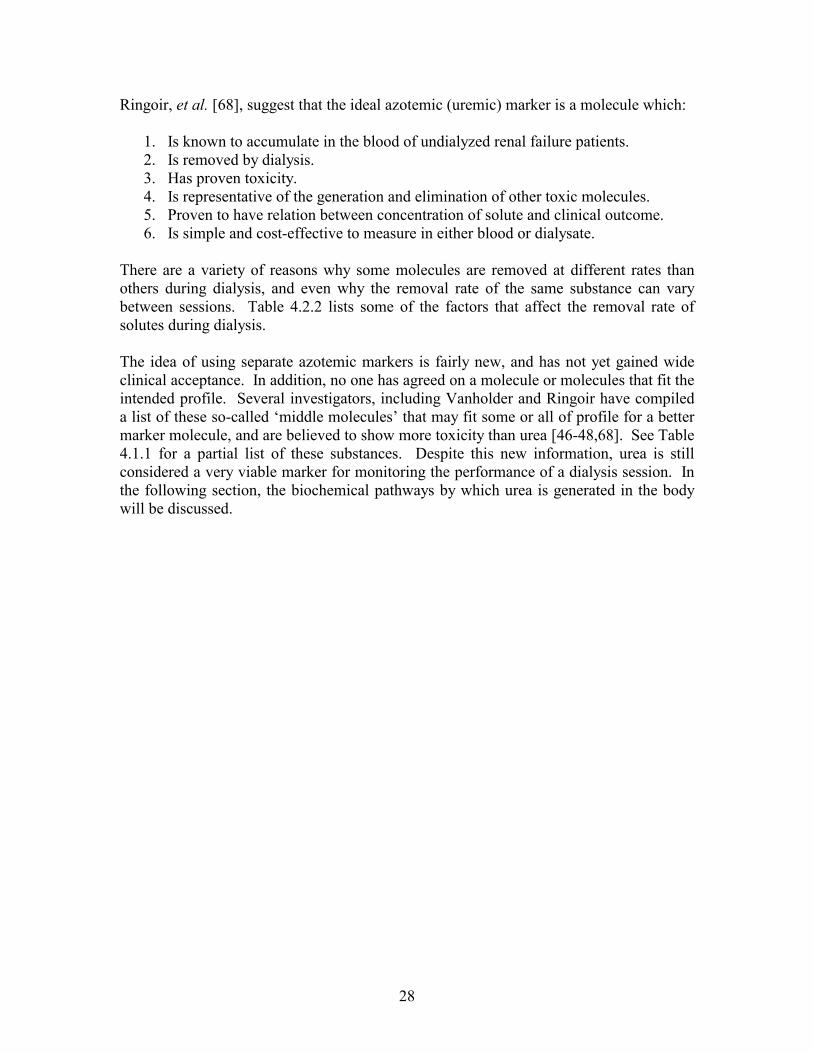
28
Ringoir, et al. [68], suggest that the ideal azotemic (uremic) marker is a molecule which:
1. Is known to accumulate in the blood of undialyzed renal failure patients. 2. Is removed by dialysis. 3. Has proven toxicity. 4. Is representative of the generation and elimination of other toxic molecules. 5. Proven to have relation between concentration of solute and clinical outcome. 6. Is simple and cost-effective to measure in either blood or dialysate.
There are a variety of reasons why some molecules are removed at different rates than others during dialysis, and even why the removal rate of the same substance can vary between sessions. Table 4.2.2 lists some of the factors that affect the removal rate of solutes during dialysis. The idea of using separate azotemic markers is fairly new, and has not yet gained wide clinical acceptance. In addition, no one has agreed on a molecule or molecules that fit the intended profile. Several investigators, including Vanholder and Ringoir have compiled a list of these so-called ‘middle molecules’ that may fit some or all of profile for a better marker molecule, and are believed to show more toxicity than urea [46-48,68]. See Table 4.1.1 for a partial list of these substances. Despite this new information, urea is still considered a very viable marker for monitoring the performance of a dialysis session. In the following section, the biochemical pathways by which urea is generated in the body will be discussed.

29
Table 4.2.2: Factors influencing solute removal during dialysis [68].
Solute Related Factors Compartmental distribution Intracellular concentration (resistance of cell membrane) Protein binding Electrostatic charge Steric configuration Molecular weight Patient Related Factors Distribution volume and body weight Intake and generation Solute Metabolic precursors Residual renal function Vascular access quality Absorption from the intestine Hematocrit Blood viscosity Dialysis Related Factors Dialysis time Interdialytic intervals Blood flow (overall and extremity) Concentration gradient Dialysate flow rate Dialyzer surface area Dialyzer volume Dialyzer membrane resistance Dialyzer pore size Adsorption (deposition of proteins or other constituents) On the membrane On other parts of the dialyzer circuit Ultrafiltration rate Intradialytic changes in efficiency Changes with indirect effect on solute related factors Blood pH Heparinization Free fatty acid concentration
4.2.7 Biochemical Pathways for the Generation of Urea The biochemical pathway by which urea is generated in the liver is well understood. When amino acids are deaminated, the resulting NH3 is cytotoxic. It must therefore be converted to another product before the process is complete. Urea is a by-product of a cyclic pathway known as the urea cycle. Most of the early work in understanding this set of reactions was done by Krebs and Henseleit in the early 1930’s. The overall stoichiometry of the urea cycle is given by the following reaction [72]:

30
CO2 + NH4
+ + 3 ATP + aspartate + 2 H2O →→→→ (4.13) urea + 2 ADP + 2 Pi + AMP + PPi + fumarate + 5 H+
The production of urea occurs from the amino acid arginine as it is regenerated to ornithine. For each turn of the urea cycle, two nitrogens are eliminated, and four high-energy phosphates are consumed. This includes the PPi group, which is subsequently hydrolyzed. Five enzymes are required, three of which are present in the cell matrix, and two of which are found in the inner mitochondrial membrane. Also associated with the process are several membrane transport proteins for ferrying the intermediates and reagents across the mitochondrial membrane [72]. A diagram of the overall urea cycle is shown in Figure 4.2.6. In the first step of the pathway, the free NH3 that is produced is converted into carbamoyl phosphate by the following reaction: NH4
+ + HCO3- + H2O + 2ATP →→→→ carbamoyl phosphate + H2PO4
- + 2ADP (4.14) Most of the energy used in the urea cycle is consumed in this step. Carbamoyl phosphate is a molecule that starts out as bicarbonate, and is phosphorylated through the action of ATP, forming carbonyl phosphate. The carbonyl phosphate is then attacked by an ammonia ion, which results in the formation of carbamate plus a phosphate ion. The carbamate is then acted upon again by a second ATP molecule. This results in the phosphorylation of the carbamate molecule, forming carbamoyl phosphate. The above reaction is completely catalyzed by the enzyme carbamoyl phosphate synthase. The reaction is shown schematically in Figure 4.2.4. The entire reaction is shown in Figure 4.2.6. Once the carbamoyl phosphate is formed in the mitochondria, it is able to interact with L-Ornithine, which is transported across the mitochondrial membrane by a carrier protein. The carbamoyl group is transferred to L-Ornithine, forming L-Citrulline. This reaction is catalyzed by the enzyme ornithine transcarbamoylase. This process also releases an inorganic phosphate molecule. L-Citrulline then combines with L-Aspartate and ATP to form Argininosuccinate. Argininosuccinate synthase is the enzyme responsible for this conversion. The ATP is converted to AMP + PPi. The high-energy phosphate is subsequently broken down, resulting in a net cost of two ATP molecules. At this point, Argininosuccinate is broken down into L-Arginine and fumarate under the influence of Argininosuccinate lyase. The L-Arginine is then hydrolyzed into urea and L-Ornithine, thereby returning to the beginning of the cycle.
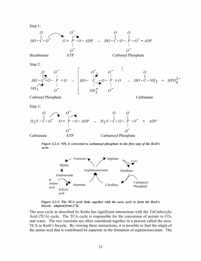
31
Step 1:
ADPO
O
O
PO
O
CHOADPO
O
O
POO
O
CHO +−−
−
−−−→−−
−
−
=−−−||
|
|||
|
||
Bicarbonate ATP Carbonyl Phosphate Step 2:
−+−−→
�
������
�
�
=
−
−
−−
−
+
−→=
−
−
−−− 242
|||
|
|
3
|
|
|
||
3
HPONH
O
CHOO
O
O
PO
O
NH
CHOO
O
O
PO
O
C
NH
HO
Carbonyl Phosphate Carbamate Step 3:
ADPO
O
O
PO
O
CNHADPO
O
O
POO
O
CNH +−−
−
−−−→−−
−
−
=−−−||
|
||2
|
|
||2
Carbamate ATP Carbamoyl Phosphate
Figure 4.2.4: NH3 is converted to carbamoyl phosphate in the first step of the Kreb's cycle.
Figure 4.2.5: The TCA cycle links together with the urea cycle to form the Kreb’s bicycle. Adapted from [72].
The urea cycle as described by Krebs has significant interactions with the TriCarboxylic Acid (TCA) cycle. The TCA cycle is responsible for the conversion of acetate to CO2 and water. The two reactions are often considered together in a process called the urea-TCA or Kreb’s bicycle. By viewing these interactions, it is possible to find the origin of the amino acid that is contributed by aspartate in the formation of argininosuccinate. The
α-Amino acid
Aspartate
Oxaloacetate
Malate
Fumarate
Argininosuccinate
Citrulline
Ornithine
ArginineUrea
Carbamoyl Phosphate
α-Keto acid

32
fumarate released by the breakdown of argininosuccinate also plays a part in this cycle. Figure 4.2.5 shows how TCA cycle and the urea cycle interact.
Figure 4.2.6: The urea cycle takes place in the cytosol and mitochondria of the liver cell. Urea is produced from the hydrolysis of Arginine. The cycle uses five enzymes (shown in italics) and consumes 4 ATP. Adapted from [72].
H COO - \ / C || C / \ - OOC H
H2N \ C=O /H2N
Fumarate
Arginino-succinate lyase
NH2|C=NH2
+
|NH|CH2|CH2|CH2|
HCNH3+
| COO-
NH3+
|CH2|CH2|CH2|
HCNH3+
| COO-
NH2|C=O|NH|CH2|CH2|CH2|
HCNH3+
| COO-
NH 3 + COO - | | C=N CH | | NH CH 2 | | CH 2 COO - | CH 2 | CH 2 |
HCNH 3 + |
COO -
Cytosol
NH 2 | C=O | O | - O P=O | O -
P i
COO -
|+ H3NCH | CH2 | COO-
AMP + PPi ATP
Argininosuccinatesynthase
Arginase
HCO3-
+NH4
+
HCO3-
+NH4
+
2 ATP 3 H + +2 ADP + P i
L-Arginine
Urea
L- Ornithine
Ornithinetranscarbamoylase
Carbamoyl phosphate
Carbamoyl phosphate synthase
L-Citrulline
Argininosuccinate
L- Aspartate
Inner mitochondrialmembrane

33
4.3 Dialysate-Side vs. Blood-Side Measurements: A history of dialysis adequacy monitoring
Since the early 1970’s, there has been a flurry of activity in the renal therapy research community aimed at finding the optimal way to dialyze a patient. Most notably, the search has focused on finding a universal parameter that tells whether or not the patient is receiving adequate therapy. A landmark study completed in 1985 by Gotch and Sargent showed that a parameter relating the clearance of the dialyzer, the time spent on dialysis, and the urea distribution volume of the patient’s body provided a strong predictor of the adequacy of dialysis [14]. This study showed that when this dimensionless parameter, known as kT/V, was greater than or equal to 1, complications from renal failure were dramatically reduced. There are many problems with making kT/V measurements in the clinical setting however. First, there is little widespread agreement on how to make the measurements, mainly stemming from differences in how to calculate the urea distribution volume. Some researchers use a constant value of 58% of body weight (55% for women). This is a simple approach, which can lead to large errors in persons with non-ideal body types [26,31,32,36-38,46,73] Other researchers use a single pool, variable volume model (VVSP), which assumes that urea is distributed only in one body compartment, but that the volume of this compartment is changing over time. The distribution volume is found using bioimpedance methods. More complicated models also exist, notably the double pool variable volume model, but these have not found widespread clinical use due to their increased complexity [20]. A third modeling method is the DDQ, direct dialysate quantification, in which all of the spent dialysate is collected over the course of a session. Since the volume can easily top 100 L per patient per session, this is impractical for large-scale operations [3,18,31,41]. A second problem involves calculation of the dialyzer clearance. This involves knowledge of many parameters, including the exact blood flow rate at the dialyzer, volume of water removed from the patient, and several measurements of the patient’s BUN (Blood Urea Nitrogen) level. The BUN level is determined from blood samples which generally must be analyzed away from the patient, preventing real time estimation of the progress of the session. This also can introduce errors due to recirculation at the fistula or urea rebound after dialysis treatment [25]. Experience has shown however that this measurement is prone to sampling errors. When blood samples are taken, they are generally taken from the same site as the blood being sent to the dialyzer. Since blood access is achieved with a two bore needle, some recirculation of blood occurs between needles, which results in mixing of the uremic vs. clean blood. The true urea value may be higher that what is obtained from the sample in this case. Another sampling problem is the timing of the sample. One sample is taken at the beginning of the session, one at the halfway point, and one at the end. The timing of the end sample is critical, because of two periods of urea rebound that are known to occur. The first occurs rapidly, within 20 seconds to 1 minute after dialysis is stopped. The second occurs more slowly, and is generally complete within 30 minutes after dialysis is stopped [25]. Ideally, the last sample should be taken after this period of time, but this is

34
a serious inconvenience to the patient and the dialysis center. This method is also expensive, both in terms of laboratory sample analysis and technician/nurse time associated with collecting the samples. For this reason, this procedure is generally only done once per week or even once per month for a given patient. This may lead to further errors if the session monitored is not typical of the rest [6]. Modeling the solution is complicated by the fact that the patient’s body is also generating new urea at all times. Measuring all of these parameters becomes a significant workload issue for the dialysis unit personnel. Once all of the important parameters have been recorded, the work is not yet done. In order to arrive at a solution, a set of equations must be solved iteratively to obtain the desired result. This must generally be done off line via computer. The complexity, work, and expense involved in obtaining these results have prevented urea kinetic modeling from finding widespread use in the clinical setting [27,37]. In recent years, two alternate parameters known as the Solute Removal Index (SRI) and the Urea Reduction Ratio (URR) have been developed. The URR is simply a ratio of pre vs. post dialysis BUN values. This is a simplified measure that can be easily calculated at bedside and requires no blood sampling. It is often considered to be inaccurate, because of the urea rebound [25]. For this reason, measurements that require blood-side BUN measurements tend to overestimate the adequacy of dialysis. The SRI is a removal rate parameter calculated from the dialysate side urea content. Experimentally, the SRI shows a double exponential characteristic, lending support to a double pool urea distribution model [5]. In addition, several authors have shown that kT/V can be calculated from dialysate-side urea measurements from the following equation:
hr
dry
D
TBW
BWTtC
VkT
01786.01
3)(ln
−
∆+∂
∂−= (4.15)
∆BW refers to the amount of fluid removed from the patient during dialysis, BWdry refers to the patient’s weight when no edema is present, CD represents the dialysate side urea concentration, and T represents the length of the dialysis session in hours. This model was developed by Garred, et al., and relies on the fact that dialysate urea has been seen to be a constant fraction of the blood urea concentration [25]. (CD = effective clearance/dialysate flow rate). The dependence of the equation on rate indicates that a semi-continuous measurement of CD is required. Minor corrections are applied to correct for change in body water and urea generation during dialysis [6,25,27]. Results of these studies are generally good for anuric (advanced renal failure) patients, but they may underestimate the value of kT/V for patients with some residual renal function [2]. The SRI is gaining widespread clinical acceptance as the method of choice for quantifying dialysis efficiency. It is subject to fewer errors than conventional blood side methods, and the calculations and measurements involved are far less involved. The method lends itself well to on-line automatic measurements.
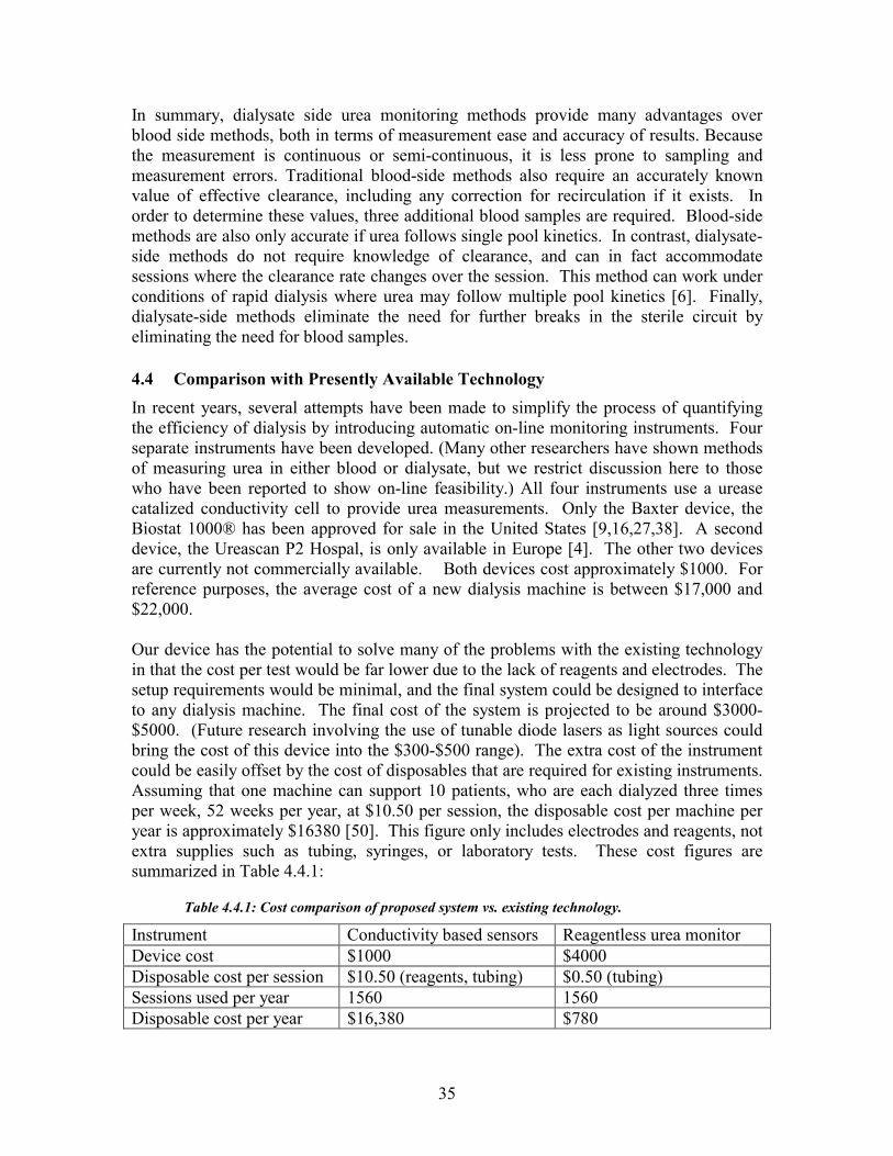
35
In summary, dialysate side urea monitoring methods provide many advantages over blood side methods, both in terms of measurement ease and accuracy of results. Because the measurement is continuous or semi-continuous, it is less prone to sampling and measurement errors. Traditional blood-side methods also require an accurately known value of effective clearance, including any correction for recirculation if it exists. In order to determine these values, three additional blood samples are required. Blood-side methods are also only accurate if urea follows single pool kinetics. In contrast, dialysate-side methods do not require knowledge of clearance, and can in fact accommodate sessions where the clearance rate changes over the session. This method can work under conditions of rapid dialysis where urea may follow multiple pool kinetics [6]. Finally, dialysate-side methods eliminate the need for further breaks in the sterile circuit by eliminating the need for blood samples.
4.4 Comparison with Presently Available Technology In recent years, several attempts have been made to simplify the process of quantifying the efficiency of dialysis by introducing automatic on-line monitoring instruments. Four separate instruments have been developed. (Many other researchers have shown methods of measuring urea in either blood or dialysate, but we restrict discussion here to those who have been reported to show on-line feasibility.) All four instruments use a urease catalized conductivity cell to provide urea measurements. Only the Baxter device, the Biostat 1000® has been approved for sale in the United States [9,16,27,38]. A second device, the Ureascan P2 Hospal, is only available in Europe [4]. The other two devices are currently not commercially available. Both devices cost approximately $1000. For reference purposes, the average cost of a new dialysis machine is between $17,000 and $22,000. Our device has the potential to solve many of the problems with the existing technology in that the cost per test would be far lower due to the lack of reagents and electrodes. The setup requirements would be minimal, and the final system could be designed to interface to any dialysis machine. The final cost of the system is projected to be around $3000-$5000. (Future research involving the use of tunable diode lasers as light sources could bring the cost of this device into the $300-$500 range). The extra cost of the instrument could be easily offset by the cost of disposables that are required for existing instruments. Assuming that one machine can support 10 patients, who are each dialyzed three times per week, 52 weeks per year, at $10.50 per session, the disposable cost per machine per year is approximately $16380 [50]. This figure only includes electrodes and reagents, not extra supplies such as tubing, syringes, or laboratory tests. These cost figures are summarized in Table 4.4.1:
Table 4.4.1: Cost comparison of proposed system vs. existing technology.
Instrument Conductivity based sensors Reagentless urea monitor Device cost $1000 $4000 Disposable cost per session $10.50 (reagents, tubing) $0.50 (tubing) Sessions used per year 1560 1560 Disposable cost per year $16,380 $780

36
While these devices have all been shown to provide acceptable accuracy in the clinical setting, they have not found widespread use. First, they are expensive to use due to the need for disposables. Second, the devices require extra maintenance and setup by the clinical personnel. Finally, the devices are often machine-specific, preventing their use in centers that do not own compatible hemodialysis equipment [50]. A summary of each device and any relevant clinical studies performed to evaluate them is given here. Baxter Healthcare, Inc. – Biostat 1000. This device, approved for use by the FDA in 1995, uses a urease-immobilized cap in a flow-through design to measure urea in spent dialysate. The sensor provides a near-continuous measure of dialysate urea content, allowing for good curve fitting, early estimation of intradialytic kT/V, and an increased precision calculation of total urea removal. The instrument also includes a bacterial filter that prevents loss of dialysate urea caused by urease producing bacteria. Independent studies using this instrument have found that it agrees well with results of traditional methods of urea kinetic monitoring such as DDQ and VVSP models [2]. Garred et al. – This sensor is also based on a flow-through cell, but instead of immobilized urease it uses a liquid form that is filled through a port with a syringe. An ammonia sensor with a calomel reference electrode is used to provide a conductivity measurement. This urea sensor provided kT/V values that were reasonably well related to blood-side kT/V measurements for four dialysis patients [26]. Jacobs et al. – In this research, the group developed a screen printed planar urea sensor. The sensor displayed acceptable accuracy of approximately 1.2 mg/dl, but its linear range was only up to 90 mg/dl, which is not enough to accurately reproduce the 6-180 mg/dl expected range. The sensor is also complicated to produce and displays a limited shelf life of five days [7]. Calzavara et al. – Ureascan P2 Hospal. This European device also utilized a standard urease flow-through cell. Its accuracy is approximately 1.3 to 2.5 mg/dl. The authors of the study note that they were unable to relate the output of their dialysis sensor to the plasma urea content [4].
4.5 Classical Absorption Spectrometry – The Beer-Lambert Law The underlying principle for using light transmission to measure analyte concentration is the Beer-Lambert Law. This law states that equal thicknesses of an absorbing medium will absorb an equal amount of light. Stated differently, the amount of light absorbed when traversing through a medium is linearly dependent on the concentration of the absorbing substance, the thickness of the sample, and a characteristic parameter called the extinction coefficient that depends on wavelength. In equation form, A(λ) = a(λ)⋅C⋅x, where A(λ) is the absorbance, a(λ) is the absorbance coefficient in units of dl/cm⋅mg, C is the concentration in mg/dl, and x is the distance in cm. Note that absorbance is the logarithm of transmittance, which is the fraction of light transmitted through the sample. Transmittance can therefore be defined as Io/Ii, or 10-a(λ)⋅C⋅x, where Ii is the transmitted

37
light intensity in Watts and Io is the light intensity at the exit of the sample. The product of the absorbance coefficient a(λ) and the concentration C is a value known as the extinction coefficient (k) of the sample, which has units of 1/cm. The transmittance of the sample can therefore be written as 10-kx. The extinction coefficient for a given molecule is a complex function of wavelength. The shape of the function depends on the vibrational, translational, and rotational characteristics of the particular molecule. Just as the mechanical systems represented by mass, spring, and dashpot models have preferred frequencies at which they will vibrate when excited, so do all molecules. These molecules will absorb some frequencies more than others as the chemical bonds become excited by the addition of light energy. This excitation will cause the bonds to stretch, twist, or vibrate, then relax. Since frequency and energy are proportional, and inversely related to wavelength, we obtain a spectrum by looking at this characteristic absorbtion over a range of wavelengths. Each molecule has its own characteristic “fingerprint” that can be used to identify it. By identifying certain characteristic bands, it is possible to discriminate one molecule from another. Optical instruments have been developed that can detect the presence of a given substance in a sample, and detect the concentration of that substance by using the Beer-Lambert Law.
4.6 The Optical Bridge When performing conventional optical measurements of physiological analytes in the near infrared, two main problems exist. First, the analyte to be measured is usually found in concentrations several orders of magnitude smaller than that of water. Second, the extinction coefficient (and hence the absorbance) of water is often several orders of magnitude larger than that of the analyte. In a conventional system, the information that relates to analyte concentration is far below the noise level of the measurement system. The problem is the extreme dynamic range of signal: In biologic samples, there is an abundance of water (that strongly absorbs in the spectral region of interest), and traces of analytes (that absorb weakly in the spectral region of interest). The result is that both the optical signal and its transduced electrical equivalent posses a huge “quasi DC” component (“background”), and a tiny variable component (“signal”). The limiting factor of the optical measurements is the present level of technology: existing measurement systems do not possess the dynamic range that would enable sufficiently accurate measurement of the “signal” in the presence of the “background”. As we would say, the information about the analyte content of the sample lies below the noise level of the system. This problem is currently solved by adding special reagents to the sample to amplify the response. These reagents react with the analyte, producing a visible color-change reaction. The new sample is then analyzed with a conventional absorption spectrophotometer. This method, while relatively simple, has several drawbacks. First, these reagents are expensive, and often quite toxic. Second, it is an added task for the personnel operating the instrument to change reagent packs every time a measurement is to be made.

38
We wish to make an automated urea measurement without the need for reagents, so we must find a way to null out the complex near-IR background spectrum that arises mainly from the water in the dialysis fluid. The Optical Bridge is a method that can be used to solve this problem. In the following section, we describe the basic principles and define the basic terms associated with its operation.
4.6.1 Definition and Principles With the technology existing in the year 2000, reagentless absorption measurements cannot be used to make determinations of biological analyte levels. For example, after the optical signal is transduced into an electrical signal, and digitized, the “background” will use approximately ¾ of the analog-to-digital converter’s full scale, e.g. 10 V. At the same time, the analyte’s contribution is only a few tens of microvolts (for urea, the extinction coefficient is 100,000 times smaller and the concentration 5000 times smaller than that of water). In order to resolve and measure 1% variations of the analyte concentration, this would require the A/D convert’s effective resolution to be over 32 bits, which is, with the existing technology, practically impossible to achieve. Therefore, mathematical manipulation of the digitized data cannot be used to extract the signal from the background, or yield any other useful information. To solve the problem, signal processing must be implemented that removes the unwanted background component at the front end, before the signal enters the section of the signal path that cannot handle the extreme dynamic range – before the optical signal is digitized. In other words, the intrinsic optical properties of the sample must be used to reduce the level of background signal inherent in the system. What we must do is to make the background optically “transparent” to the system; make it contribute little or not at all to the overall signal. This way, the resultant AC signal can now be sufficiently amplified, so that the required resolution can be achieved.
The Optical Bridge is similar to the well-known Wheatstone bridge, which is often used to make strain gauge and other measurements. A strain gauge has a static resistance distributed evenly across the four “arms” of the bridge. The output of the Wheatstone bridge is fed to a differential amplifier. When no load is applied, the Wheatstone bridge is “balanced” – all four arms have the same resistance, and therefore the Wheatstone bridge amplifier has a zero output voltage, regardless of the size of the resistance per arm. When a load is applied across one pair of the arms, their resistance changes slightly, yielding an output from the bridge amplifier that is directly proportional to the resistance change. A conventional amplifier cannot readily detect this small change in resistance when it is accompanied by a large common mode signal, but the Wheatstone bridge output only produces differential signals caused by changes in the resistance of the arms of the bridge. The Optical Bridge is designed to overcome a similar problem. As explained previously, it is not possible to detect a small signal caused by a change in urea concentration in the presence of the large background water signal. Therefore, a null balanced method is applied. While the Wheatstone bridge uses a differential amplifier to measure small changes in resistance across the arms of the strain gauge, the Optical Bridge measures the difference in light transmission between two wavelengths across the sample. To continue

39
the analogy to the Wheatstone bridge, the absorbance at each measurement wavelength of the Optical Bridge can be likened to the resistance of each arm of the Wheatstone bridge. Small changes in absorption caused by the addition of analyte cause a proportional change in the output signal, regardless of the overall absorbance of the system. The measurement wavelengths are selected to fulfill two criteria:
1. The analyte should have a different absorption at each wavelength, preferably strong at the principal wavelength and weaker at the reference wavelength.
2. The background must have the same absorption at both wavelengths.
The output AC signal is proportional to the difference in the intensity of the transmitted light recorded at the two wavelengths. When the wavelengths are selected according to the listed criteria, the output signal is proportional to the analyte concentration only. If there is no analyte in the optical path, the signal is zero. As the analyte concentration increases, so does the AC signal. Figure 4.6.1 illustrates this principle.
Figure 4.6.1: The Reference and Principal wavelengths are selected according to the criteria stated in §4.4.1. With no analyte present, the output signal, represented by the line connecting the absorbance at the two wavelengths is zero. This is true even when the sample thickness changes. When the analyte is present, the absorbance at the Principal wavelength changes, causing a change in the output signal. This change is shown greatly magnified in the figure.
We have stated that the Optical Bridge is capable of nulling out a background signal from the sample by measuring the difference in light transmission at pair of wavelengths. The measurement is more than a simple subtraction of two absorbance measurements, since this would involve analog to digital conversion of the entire sample. (background + analyte). This would result in a large quantization noise, effectively obscuring the desired signal. Instead, the background component is eliminated prior to data acquisition, so that a larger gain can be used and therefore a larger signal to noise ratio can be achieved. Since the composition of the background is variable, the best wavelengths for effectively “balancing out” the background are selected in real time during each measurement.
Wavelength
Transmittance
Reference Principal
No Analyte
Analyte Present

40
The first major problem is due to the fact that the exact composition of a physiological sample is unknown. For this reason, it is impossible to select, either theoretically or empirically, the best pair of wavelengths to use for any one measurement. The best solution to this problem is to design the system such that it selects its own wavelengths in order to “balance out” the absorbance of the undesired background. This indicates that the system must also have some means of performing measurements separately on the background (without the presence of the analyte being measured). (The method for doing this will be described in §5.2). First, the Principal wavelength is chosen empirically by using known absorbance peaks for the analyte. Then, with only the background fluid in the optical path, the system performs a series of measurements to select the ideal Reference wavelength (while the Principal wavelength is held constant). When the optimal Reference Wavelength has been identified (thus balancing out the background), the analyte is allowed to re-enter the optical path, and the analysis takes place. In this way, the large undesired background absorbance is removed from the signal, allowing a large degree of AC amplification to be applied to the desired signal without saturating the system. This measurement technique has two distinct stages. The first stage is called balancing, and the second stage is measuring. During balancing, as described previously, the optical path only contains clean dialysis fluid, the “background” for the measurement. A beam of nearly monochromatic light, alternating between the Principal and Reference wavelengths, is directed into the sample. See Figure 4.6.3. This beam is generated using an Acousto Optical Tunable Filter (AOTF), which is manufactured by Brimrose Corporation (Baltimore, MD). Appendix F includes a description of AOTF’s. This device acts as a rapidly tunable narrow bandpass filter for a light source, which is a 100 W halogen lamp. A radio-frequency signal is applied to the AOTF that controls both the intensity and the wavelength of the light. The light is amplitude and frequency modulated at 60 Hz producing, a two-phase beam at the Reference and Principal wavelengths. During the first phase, the transmitted light consists of the Principal wavelength, and during the second phase, it consists of the Reference wavelength. At the entrance to the sample, the light intensity of the two phases of the beam is equal. Initially, at the exit of the sample, one phase of the beam will be attenuated more than the other. See Figure 4.6.2. During the balancing stage, the Principal wavelength (which is absorbed by urea) is held constant, and the reference wavelength is adjusted until the exit intensities are the same for both phases (or wavelengths). This can be explained graphically by examining

41
Figure 4.6.1. The bottom curve represents a typical spectrum of dialysate in water. The balancing process can be represented graphically by the shifting of the reference wavelength left or right until the line connecting the two wavelengths is parallel to the x axis. When this is achieved, the system is considered balanced, and the measurement stage can begin. The real time nature of this procedure accounts for possible changes in the composition of the fluid or temperature of the fluid from measurement to measurement, rather than relying on a fixed set of wavelengths. At the end of this balanced stage, the output signal is approximately zero. At this point, we introduce a notation convention. Data that is recorded from the instrument during the balancing phase of the measurement is given the suffix 00. Data that is recorded from the instrument during the measuring phase is given the suffix 1. Therefore, the AC signal during the balancing phase is represented by AC00, while the AC signal during the measuring phase is represented by AC1. Additionally, the term position 00 is used to represent the compressed state of the sample during the balancing phase. The term position 1 is used to represent the uncompressed state of the sample during the measuring phase. The output signal itself is actually obtained from a lock in amplifier (LIA) that is tuned to the wavelength chopping frequency. A LIA consists of a phase sensitive detector that is followed by a low-pass filter. The LIA outputs a signal that is proportional to the difference between the two phases of its input. During balancing, the system adjusts the reference wavelength to minimize this signal. The input to the LIA at the beginning of the balancing phase is roughly a small amplitude square wave. At the end of balancing, the amplitude of the square wave is very small. (Ideally, it is zero, but this cannot be achieved in practice due to noise). Once the analyte is allowed to enter the path, the sample absorbance at the principle wavelength, which responds to the presence of urea, increases, and the AC signal becomes large. This signal is then recorded. This process is demonstrated in Figure 4.6.2.
Figure 4.6.2: The Optical Bridge input signal during three phases of the measurement.
When the measurement process begins, the optical path is changed, allowing the spent dialysate into the sample path. The mechanism for this operation is described in Appendix E. The addition of this “incremental sample” causes a change in the output signal that is proportional to the analyte concentration. The term incremental sample refers to the addition of the portion of the sample that contains the analyte.
prior to balancing balancing complete urea added, bridge unbalanced

42
Geometrically, the incremental sample is located next to the background sample that contains no analyte – see Figure 4.6.3. Once the measuring stage begins, the optical path contains both the background and incremental analyte sample. At this point, the light intensity exiting the background is equal for both wavelengths, because the wavelengths have been selected so that the background attenuates both phases of the transmitted light equally. So, the intensity of light at the entrance to the incremental sample is the same for both wavelengths. The only thing that can contribute to an unequal attenuation of either wavelength phase is the presence of the analyte in the optical path. While it is true that certain substances can interfere with this measurement, it should be possible to avoid this effect by careful selection of wavelength pairs and possibly by using multiple wavelength pairs. The measurements resulting from the use of other wavelength pairs could be used to extract the urea signal from the undesired analyte by regression analysis, deconvolutions, or other similar techniques. This would involve careful studies of how the interfering analyte affects the measurement at both sets of wavelengths, and the development of a mathematical model based on the analysis of the experimental data. §4.8 discusses the possible effects of interfering substances on the measurement. Figure 4.6.3 shows a schematic diagram of the balancing and measurement stages and the light intensity at each position in the sample.
Figure 4.6.3: Light intensity at the entrance and exit of the sample is represented for each wavelength phase by the length of the arrow. It is always equal entering the sample. In (a), prior to balancing; the light intensity at the exit is unequal. At (b), after balancing, the light intensity for both phases is the same. In (c), the measurement stage has begun, and the spent dialysate sample is included. The light intensity exiting the clean sample is equal, but it is different after exiting the spent “incremental sample”.
4.6.2 Ideal Mathematical Model for the Optical Bridge The Optical Bridge signal, S, is equal to the difference between the signal power at the two measurement wavelengths. During balancing, where the sample is most tightly compressed, the analyte has been squeezed from the sample. Since there is no analyte in the optical path, the AC signal will be zero:
S00 = ∆P = Pλ1 – Pλ2 = 0 ( 4.16 ) During the measuring phase, where the sample has been uncompressed, and the analyte has re-entered the optical path, there is a non-zero signal. The absorption coefficient k over the sample has now changed by some ∆k due to the resulting addition of analyte when the sample is uncompressed. The signal can now be represented by:
Clean
Clean
Clean
Spent
(a) (b) (c)

43
S1 ≠ 0 = P0 [10-(k-∆k)⋅x – 10-k⋅x] = P0 10-k⋅x [10∆k⋅x - 1] ( 4.17 )
=
∆k·x « 1, so it is possible to use a well-known Taylor series approximation: 10∆k⋅x = 1 + ∆k⋅x ( 4.18 )
So, in the final form, the signal is represented by:
S1 = P0⋅∆k⋅x⋅10-k⋅x ( 4.19 )
The ∆k term is directly related to the analyte concentration, and Equation 4.19 demonstrates that the signal obtained from this system is directly related to this term. The signal is also affected by the power incident on the sample, the pathlength traversed in the sample, and the logarithmic reduction in signal power due to Beer’s law. Equation 4.19 can be solved for ∆k to obtain the following result:
xkxPSk ⋅−⋅⋅
=∆101
0
( 4.20 )
In order to obtain a concentration estimate from ∆k, a two-point calibration may be used. This involves the linear fit of two sample concentrations to obtain slope and intercept information. The slope should be related to the difference in extinction coefficients for the analyte in question between λ1 and λ2. This mathematical model is for an ideal system, and it therefore has somewhat limited application in practice. Chapters 5 and 7 describe this system in greater detail, and propose compensations for this algorithm that are required for it to function in the presence of noise and other complicating factors.
4.6.3 Application of the Optical Bridge to Urea Measurements in Dialysate The Optical Bridge technique has undergone several years of development in the area of non-invasive monitoring of blood glucose for diabetics. For this measurement, a capillary-rich site such as the earlobe is used. The glucose is assumed to reside mainly in the blood, and the system is balanced by gently squeezing the tissue to displace blood and glucose from the measurement site. Once balancing is complete, the squeeze is relaxed, and the measurement takes place. While it has been assumed, since the inception of this approach that it is possible to measure other analytes with this method, only glucose research has been done in that area with the exception of this thesis. Two major obstacles must be overcome when attempting to measure a new analyte with this method. First, a method of separating the background from the analyte must be determined, similar to the technique of squeezing blood out of the tissue to displace glucose. For in vivo measurements, this involves determining whether or not tissue squeezing displaces the substance in question. For our application, this measurement is performed on spent dialysate, rather than tissue, thus we have a natural background in the clean dialysis fluid.

44
Second, a pair of measurement wavelengths must be found that satisfies the wavelength criteria. This can be done by dissolving high concentrations of urea in water or dialysis fluid, and analyzing them with a conventional spectrophotometer. By making a series of measurements on increasingly diluted samples, it is possible to find wavelengths at which the absorbance is strongly dependent on urea concentration. These wavelengths become the potential Principal wavelengths. By looking only at clean dialysate, we then attempt to find other wavelengths where the absorbance is equal (isoabsorbance) to the Principal wavelength. These wavelengths become the Reference wavelengths. It should be noted that the Reference wavelength selected by this method is only a starting point for the adaptive balancing algorithm. As has been described in this section, the Reference wavelength is actually selected automatically each time during the balancing stage of the measurement.
4.7 The Near-IR Absorbance Characteristics of Urea and Water In this section, we will discuss the IR absorption spectrum of urea in terms of its functional groups, in order to support our hypothesis that energy at 1486 nm can be used to measure urea. Urea (CN2H4O) is a single carbon molecule that is derived from the breakdown of protein. It consists of two amide (R-CONH2) functional groups. There are two main absorptions due to the amide groups. The first is a carbonyl (C=O) stretching vibration occurring at 5945 nm (1682.1 cm-1), known as the amide I band. This frequency is slightly higher than for other carbonyls due to resonance effects with the NH2 group. The second band, known as the amide II band, is derived from N-H bending, and occurs at 6254 nm (1599.1 cm-1). A weaker absorption band occurs at 6640 nm (1506.1 cm-1) due to an interaction between the N-H bending and the C-N stretching. The C-N stretch itself gives rise to a very weak band near 7143 nm (1400 cm-1). Finally, a broad, medium strength band between 16 and 23 nm (660 and 440 cm-1) occurs due to out-of-plane N-H wagging. The amine group shows two bands due to N-H stretching vibrations. The first occurs at 2906 nm (3440.6 cm-1), and the second occurs at 2914 nm (3234.2 cm-1). The first is due to a symmetrical stretch, and the second is due to an asymmetrical stretch of the N-H bond. The amine group also gives rise to an N-H bending vibration at approximately 6173 nm (1620 cm-1), but this peak is almost completely merged with the N-H bending band of the amide group. N-H wagging also occurs in this group, but it is blended with the N-H wagging of the amide group. Finally, a C-N stretching vibration also gives rise to a band at 8658 nm (1155 cm-1). We have determined that urea is sensitive to energy at 1486 nm. This is the fourth harmonic of the carbonyl band at 5945 nm. The carbonyl band was chosen because it is a characteristically strong, stable peak. In addition, this peak is shifted to a relatively unique position due to the N-H resonances on either side of the C=O bond, which is an important consideration in the specificity of the measurement. The fourth harmonic was chosen for a number of reasons, mainly having to do with optical hardware considerations. We require a source of radiation which:

45
• = Has a narrow linewidth • = Is rapidly tunable • = Preferably has no moving parts • = Can be acquired at a reasonable cost
As has been discussed elsewhere, the device that best fits these requirements is an AOTF. The upper range of AOTF operation is approximately 4500 nm. As the operating range increases, the spectral resolution becomes worse. The operating range of the AOTF used in this research is 1200-1800 nm, where the spectral resolution is approximately 2 nm. Indium Gallium Arsenide (InGaAs) detectors have a fairly low noise level and function in the same spectral region. Urea still has a reasonable absorption at the fourth harmonic (it decreases by approximately a factor of four from the primary band), so this represents the ideal tradeoff in terms of available hardware. The chosen urea peak lies on the side of a steep water peak that is the third harmonic of an O-H bending band. In dialysate, the nearest balance point to the 1486 nm occurs at approximately 1393 nm. This wavelength will vary with sample composition at measurement time.
4.7.1 Optical Characteristics of Absorbing Substances in the near-IR Here we explore how overtone bands in the near-IR arise from fundamental absorption bands in the mid-IR. Using water as an example, we will show how the magnitude and bandwidth of the relevant bands are changed as the wavelength decreases into the near-IR. The fundamental water absorption band (caused by an OH stretch) occurs at approximately 3500 cm-1 (2891 nm). It has a bandwidth of approximately 340 nm. This curve can be seen below in Figure 4.7.1.
Figure 4.7.1: Absorbance spectrum for water in the mid-IR.
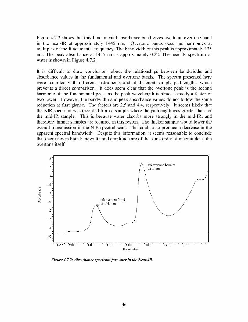
46
Figure 4.7.2 shows that this fundamental absorbance band gives rise to an overtone band in the near-IR at approximately 1445 nm. Overtone bands occur as harmonics at multiples of the fundamental frequency. The bandwidth of this peak is approximately 135 nm. The peak absorbance at 1445 nm is approximately 0.22. The near-IR spectrum of water is shown in Figure 4.7.2. It is difficult to draw conclusions about the relationships between bandwidths and absorbance values in the fundamental and overtone bands. The spectra presented here were recorded with different instruments and at different sample pathlengths, which prevents a direct comparison. It does seem clear that the overtone peak is the second harmonic of the fundamental peak, as the peak wavelength is almost exactly a factor of two lower. However, the bandwidth and peak absorbance values do not follow the same reduction at first glance. The factors are 2.5 and 4.4, respectively. It seems likely that the NIR spectrum was recorded from a sample where the pathlength was greater than for the mid-IR sample. This is because water absorbs more strongly in the mid-IR, and therefore thinner samples are required in this region. The thicker sample would lower the overall transmission in the NIR spectral scan. This could also produce a decrease in the apparent spectral bandwidth. Despite this information, it seems reasonable to conclude that decreases in both bandwidth and amplitude are of the same order of magnitude as the overtone itself.
Figure 4.7.2: Absorbance spectrum for water in the Near-IR.

47
4.7.2 Reflectance spectrum of urea in the NIR Figure 4.7.3 shows a curve of the reflectance of dry urea in the near-IR. Note the absorbance band centered at 1485 nm, which is an overtone of the fundamental carbonyl stretch band at 5945 nm. The aqueous spectrum displays similar features.
Figure 4.7.3: Reflectance spectrum for dry urea in the Near-IR.
4.8 Analysis of Potential Interfering Substances In this section, we will discuss the potential effects of other organic solutes on the measurement of urea in dialysate by optical means. A list of potential interferences will be identified and grouped by category. Whenever possible, the identifying IR characteristics of these molecules will be presented. Molecules or groups of molecules that have similar absorbance characteristics to urea will then be identified. If they are present in dialysate at a significant concentration level, they will be considered to be potential interferents. Note that inorganic ions will not be considered, as they do not vibrate strongly in the region of interest. The first step in this analysis is to determine what the composition of spent dialysate is. Many of the molecules making up spent dialysate are well known to physicians and researchers. Others have simply been termed “middle molecules”. Their molecular weights have been determined by mass spectrometry or gas chromatography [64,67,70]. These middle molecules have not been structurally identified, but are widely believed to be protein fragments and amino acid chains. Table 4.8.1 shows a listing of the categories of substance contained in dialysate, and examples of compounds in each category where appropriate. IR Spectra of most of these compounds were obtained from the Aldrich FT-IR Spectral Library [74]. In some cases, spectra were not available. These compounds appear in

48
italic type in Table 4.8.1. For those compounds, the spectral characteristics were estimated from principles of IR analysis [75,76]. For each compound, the following data was recorded:
• = Name • = Chemical structure • = Molecular weight • = Maximum absorbance value at each significant peak • = Absorbance value at 5945 nm (since this wavelength is hypothesized to be urea-
sensitive). We are using the primary absorbtion wavelength rather than the overtone absorbtion wavelength because it is not possible to measure the absorbance of many of these compounds at the overtone wavelength.
• = Unit absorbance value: Defined as the absorbance value per mg/dl (Calculated from the spectrum on the basis of solute/solvent mole fraction and Beer’s Law)
• = Mean concentration in dialysate. While mean concentrations of many of these substances vary widely among uremic patients, the values should be appropriate to an order of magnitude at least.
From this information, a sensitivity factor was derived. This number is the unit absorbance value multiplied by the mean dialysate concentration. From this, we can determine which molecules or categories of molecules are likely to interfere with our measurement. Figure 4.8.2 shows the relative magnitude of the sensitivity factor of possible interfering substances to that of urea. This graph is plotted logarithmically, since the sensitivity factors for all other substances are orders of magnitude smaller than that of urea. The data used to arrive at the sensitivity factors for these compounds can be found in Appendix E.
Table 4.8.1: List of potential interferents in spent dialysate. Compounds for which spectra are not available are in italics.
Substance/Category Example (if applicable) Urea Guanidines Methylguanidine, guanidine, β-guanidinopropionic acid,
Guanidinosuccinic acid, γ-guanidinobutyric acid, Taurocyamine, Creatinine, Creatine, Arginic acid, Homoarginine, N-α-acetylarginine
Phenols o-cresol, p-cresol, benzyl alcohol, phenol, tyrosine Phenolic acids P-Hydroxyphenylacetic acid, β-(m-Hydroxyphenyl)-Hydracrylic
acid Hippurates p-Hydroxyhippuric acid, o-Hydroxhippuric acid, Hippuric acid Benzoates Benzoic acid Polypeptides β2-microglobulin Indoles Indol-3-acetic acid, Indoxyl sulfate, 5-Hydroxyindol acetic acid,
Indol-3-acrylic acid, 5-Hydroxtryptophol, N-acetyltryptophan, Tryptophan
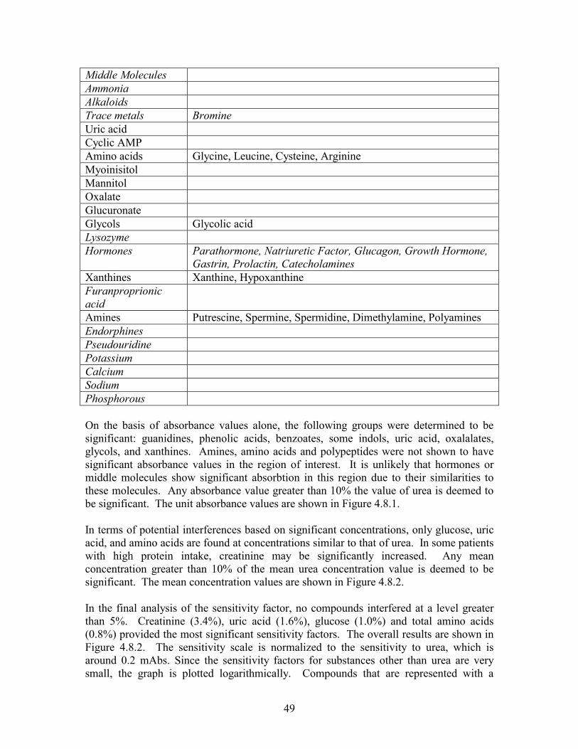
49
Middle Molecules Ammonia Alkaloids Trace metals Bromine Uric acid Cyclic AMP Amino acids Glycine, Leucine, Cysteine, Arginine Myoinisitol Mannitol Oxalate Glucuronate Glycols Glycolic acid Lysozyme Hormones Parathormone, Natriuretic Factor, Glucagon, Growth Hormone,
Gastrin, Prolactin, Catecholamines Xanthines Xanthine, Hypoxanthine Furanproprionic acid
Amines Putrescine, Spermine, Spermidine, Dimethylamine, Polyamines Endorphines Pseudouridine Potassium Calcium Sodium Phosphorous On the basis of absorbance values alone, the following groups were determined to be significant: guanidines, phenolic acids, benzoates, some indols, uric acid, oxalalates, glycols, and xanthines. Amines, amino acids and polypeptides were not shown to have significant absorbance values in the region of interest. It is unlikely that hormones or middle molecules show significant absorbtion in this region due to their similarities to these molecules. Any absorbance value greater than 10% the value of urea is deemed to be significant. The unit absorbance values are shown in Figure 4.8.1. In terms of potential interferences based on significant concentrations, only glucose, uric acid, and amino acids are found at concentrations similar to that of urea. In some patients with high protein intake, creatinine may be significantly increased. Any mean concentration greater than 10% of the mean urea concentration value is deemed to be significant. The mean concentration values are shown in Figure 4.8.2. In the final analysis of the sensitivity factor, no compounds interfered at a level greater than 5%. Creatinine (3.4%), uric acid (1.6%), glucose (1.0%) and total amino acids (0.8%) provided the most significant sensitivity factors. The overall results are shown in Figure 4.8.2. The sensitivity scale is normalized to the sensitivity to urea, which is around 0.2 mAbs. Since the sensitivity factors for substances other than urea are very small, the graph is plotted logarithmically. Compounds that are represented with a

50
diamond symbol in Figure 4.8.2 were determined to have absorbance peaks near that of urea.
0
20
40
60
80
100
120U
rea
Glu
cose
1-M
ethy
lgua
nidi
neG
uani
dine
Cre
atin
ine
Cre
atin
eAr
gini
neH
omoa
rgin
ine
Phen
olo-
Cre
sol
p-C
reso
lBe
nzyl
alc
ohol
Tyro
sine
3-H
ydro
xyph
enyl
acet
ic a
cid
o-H
ydro
xyhi
ppur
ic a
cid
Hip
puric
aci
dBe
nzoi
c ac
idIn
dol-3
-ace
tic a
cid
5-H
ydro
xyin
dol-3
- ace
tic a
cid
Indo
l-3-a
cryl
ic a
cid
5-H
ydro
xytry
ptop
hol
N-a
cety
ltryp
toph
anTr
ypto
phan
Uric
aci
dC
yclic
AM
PAm
ino
acid
s (e
.g. g
lyci
ne)
Man
nito
lO
xala
teG
lucu
rona
mid
eG
lyco
lsXa
nthi
neH
ypox
anth
ine
Putre
scin
eSp
erm
ine
Sper
mid
ine
Dim
ethy
lam
ine
conc
entr
atio
n, m
g/dl
0.0E+00
5.0E-07
1.0E-06
1.5E-06
2.0E-06
2.5E-06
3.0E-06
3.5E-06
4.0E-06
unit
abso
rban
ce, A
bs/m
g/dlUnit absorbance (per 1 mg/dl)
average concentration (mg/dl)
Figure 4.8.1: This bar graph shows the unit absorbance (per mg/dl) of many potential interferents in the spent dialysate fluid. The mean concentration of each substance in dialysate is superimposed on the graph as a line plot. The mean concentration figures are those for a typical dialysis patient.
Since we are actually using harmonics of the 5945 nm band, it is necessary to check if the interfering substances may also have harmonics occurring at or near 1485 nm. In the Figure 4.8.3, the desired urea measurement wavelength is marked with large square symbol. Harmonics of bands attributed to other compounds are represented as triangular symbols (2nd harmonic) and diamond symbols (4th harmonic). There are a few bands within a ±5 nm range of 1485 nm. These bands can be attributed to: o-cresol, benzyl alcohol, benzoic acid, and cyclic AMP. None of these compounds appear at a high enough concentration relative to urea to significantly affect the measurement, and their sensitivity factors are at least 10,000 times below that of urea. For this reason, the analysis was not repeated at the reference wavelength. The effects of water absorbance will overshadow all other absorbers at that point.

51
Sensitivity Factor
-10
-9
-8
-7
-6
-5
-4
-3
-2
-1
0U
rea
Glu
cose
1-M
ethy
lgua
nidi
neG
uani
dine
Cre
atin
ine
Cre
atin
eA
rgin
ine
Hom
oarg
inin
ePh
enol
o-C
reso
lp-
Cre
sol
Ben
zyl a
lcoh
olTy
rosi
ne3-
Hyd
roxy
phen
ylac
etic
aci
do-
Hyd
roxy
hipp
uric
aci
dH
ippu
ric a
cid
Ben
zoic
aci
dIn
dol-3
-ace
tic a
cid
5-H
ydro
xyin
dol-3
- ace
tic a
cid
Indo
l-3-a
cryl
ic a
cid
5-H
ydro
xytry
ptop
hol
N-a
cety
ltryp
toph
anTr
ypto
phan
Uric
aci
dC
yclic
AM
PA
min
o ac
ids (
e.g.
gly
cine
)M
anni
tol
Oxa
late
Glu
curo
nam
ide
Gly
cols
Xan
thin
eH
ypox
anth
ine
Putre
scin
eSp
erm
ine
Sper
mid
ine
Dim
ethy
lam
ine
Log
of S
ens.
Fact
or
Figure 4.8.2: This graph shows the logarithm of the sensitivity factor of each compound. All compounds not listed have sensitivity factors that are more than an order of magnitude lower than urea. Compounds that have harmonic absorption bands near that of urea are marked with diamonds on the figure.

52
1400
1410
1420
1430
1440
1450
1460
1470
1480
1490
1500
Ure
aG
luco
se1-
Met
hylg
uani
dine
Gua
nidi
neC
reat
inin
eC
reat
ine
Arg
inin
eH
omoa
rgin
ine
Phen
olo-
Cre
sol
p-C
reso
lB
enzy
l alc
ohol
Tyro
sine
3-H
ydro
xyph
enyl
acet
ico-
Hyd
roxy
hipp
uric
aci
dH
ippu
ric a
cid
Ben
zoic
aci
dIn
dol-3
-ace
tic a
cid
5-H
ydro
xyin
dol-3
- ace
ticIn
dol-3
-acr
ylic
aci
d5-
Hyd
roxy
trypt
opho
lN
-ace
tyltr
ypto
phan
Tryp
toph
anU
ric a
cid
Cyc
lic A
MP
Am
ino
acid
s (e.
g. g
lyci
ne)
Man
nito
lO
xala
teG
lucu
rona
mid
eG
lyco
lsX
anth
ine
Hyp
oxan
thin
ePu
tresc
ine
Sper
min
eSp
erm
idin
eD
imet
hyla
min
eW
ater
wav
elen
gth
4th harmonic3rd harmonic2nd harmonic
Figure 4.8.3: This graph shows the location of harmonics bands of potential interferents. These Near-IR harmonic bands are derived from fundamental bands in the IR. Several compounds show peaks near the desired urea peak, (those that appear within the band on the figure) but do not appear in dialysate at a concentration that could interfere with the measurement. These compounds are also identified on the sensitivity graph, Figure 4.8.2.
4.9 Multiple Linear Regression MLR is a powerful tool that requires careful application. It assumes that a linear relationship exists between a dependent variable Y and k independent variables X1, X2, …, Xk [77]. Stated differently:
yj = β0 + β1x1j + β2x2j + ⋅⋅⋅ + βkxkj + ej, (4.21) Here, ej is the deviation of the regression from the actual value of yj and βj are the individual weighting coefficients for the independent variables. In order to obtain the partial regression coefficients β0:βk, the method of partial least squares is used. The sum of the squared deviations of the observed Y vs. the value obtained from the regression equation is minimized [77]. In equation form, this means that we select β0:βk such that the following expression is minimized:
( )−−−−= 22110
2kjkjjjj xxxye βββ � (4.22)

53
This quantity is referred to as the sum of squares of the residuals (SSR). It is written in short form as: − 2)ˆ( yy j (4.23) This equation can then be solved by any convenient means to obtain the partial regression coefficients [77]. Once the partial regression coefficients have been obtained, they must be evaluated for significance to the data both individually and collectively. We need to know if each individual variable makes a statistically significant contribution to the overall model, and whether or not the overall model is not only a good fit of the data, but is also statistically significant. To test the goodness of fit, we calculate the coefficient of multiple determination according to the following formula [77]:
−
−= 2
22
)()ˆ(
..1 yyyy
Rj
y k (4.24)
The quantity in the numerator of equation 4.24 is known as the explained sum of squares. It represents the sum of squares of the deviation of the calculation from the mean value of y (SSE). The quantity in the denominator is called the total sum of squares (SST). It represents the sum of squares of the deviation of each individual y from the mean value of y. Therefore, the quantity Ry1…k
2 is a measure of what percent of the variation in the data can be explained by the regression. In order to evaluate the significance of the model, a hypothesis test is performed. The null hypothesis, H0, is that β0 = β1 = … = βk = 0, or that none of the variables are of value in explaining the variation in Y. The alternate hypothesis, HA, is that not all βk = 0. An ANOVA (Analysis of Variance) table can then be constructed for the regression1:
Table 4.9.1: Analysis of Variation (ANOVA) Table
SOURCE SS d.f. MS V.R. Due to Regression
SSR k MSR = SSR / k MSR / MSE
About Regression
SSE n – k – 1 MSE = SSE / (n – k – 1)
Total SST n – 1 H0 should be rejected if the value of the variance ratio (V.R.) is greater than the critical value of the F statistic for k and n-k-1 degrees of freedom. If H0 is rejected, then we can conclude that the regression model is a good fit to the data. The individual variables can
1 (SS = Sum of Squares, d.f. is the degrees of freedom, k is the number of variables, n is the number of data points, MS is mean square, V.R. is variance ratio, SSR is the regression (explained) sum of squares, SSE is the error (unexplained) sum of squares.

54
also be checked for goodness of fit with a student’s T test. The computer program that does the analysis (in this case Microsoft Excel™) returns both the coefficient (βk) and the standard error (sek) for each variable. The t statistic is βk/sek. The variable is significant if t is greater than tcritical at the chosen level of significance [77]. When developing a model based on the MLR approach, there are several pitfalls that must be approached carefully. First, it would be very easy to “overfit” the data. Obviously, if a large number of variables are fit to a small amount of data, the model carries very little statistical weight. A general rule of thumb is that the number of data points should be at least three times greater than the number of variables [77]. Second, it is important that the variables that are fit to the data “make sense” given the functioning of the system. In other words, the selection of a variable for inclusion in the model should have logical reasoning behind it. This reduces the risk of developing a statistically insignificant model. Finally, the regression statistics must be considered carefully. Each variable should be checked for significance to the model using a student’s t test, and the significance of the overall regression should be tested using analysis of variance (ANOVA).
4.10 Summary of Background Information It is possible to draw a number of conclusions from the material presented in the previous sections of this chapter, and from the literature. These include: • = There are a number of physiological manifestations of kidney failure, and a number
of metabolic causes. Kidney failure may be acute or chronic. Cases of acute kidney failure may often be cured, while chronic kidney failure is usually degenerative and permanent. Both types of kidney failure are eventually fatal if not treated promptly.
• = Dialysis is a viable method of substituting or assisting the function of ailing or diseased kidneys. Hemodialysis and peritoneal dialysis are two of the most common methods of renal function replacement therapy.
• = When dialysis is used to replace the function of failed kidneys, changes in urea concentration are the most obvious physiological change.
• = Presently, there is no dialysis monitoring technique that satisfies the major requirements for a clinically accepted and useful instrument.
• = Many investigators have shown that urea concentrations in blood and spent dialysis fluid correlate with the expected prognosis of dialysis patients.
• = The Optical Bridge presents a viable method of monitoring concentrations of physiological analytes without reagents or user intervention.
• = It is possible to develop a mathematical model relating the output of the instrument to the concentration of urea in spent dialysate.
• = Urea levels in spent dialysate present a good estimator of the performance of the dialysis session

55
5 DIALYSIS EFFICIENCY MONITORING SYSTEM DESIGN OVERVIEW
In this chapter, we begin by introducing the design process that was undertaken in the construction of this Optical Bridge based system. Some of the more advanced topics concerning the operational principles of this technique are discussed as well. At the most basic level, the dialysis monitoring instrument must direct a beam of light into the dialysate sample and record the amount of light exiting the sample. This light signal must be converted to an electrical signal, amplified and filtered, and converted to a digital signal so that it may be processed by a special software algorithm. The block diagram of the system is shown in Figure 5.1.1. The details of these subsystems are described in the Appendices.
5.1 Design Overview In order to obtain a sufficiently accurate measure of urea concentration using an optical method, it is necessary to balance out the much larger absorbance signal that arises from the rest of the sample matrix (background) - See §4.6. This section describes a measurement that relies on the selection of two wavelengths. The absorption at one of these wavelengths, the Principal wavelength, is sensitive to the presence of urea. The other wavelength, the Reference wavelength, is automatically tuned during the measurement to achieve exactly the same absorbance (isoabsorbance) in the background as with the Principal wavelength. The system output signal, which is proportional to the difference in sample absorbance between the two wavelengths, is therefore able to nullify the contribution of the background signal. All that is left is the signal from the desired analyte, urea, which can then be amplified and processed sufficiently to yield an accurate measurement. Refer to §4.6 for a more complete discussion of the Optical Bridge. It is necessary to decide upon a starting point in the explanation of the system. Since we have stated that the main function of the system, at its most basic level, is to monitor light transmission, we will begin at that point. The light that has passed through the sample (i.e. the light that was not absorbed by the sample) hits a photodetector and is converted to an electrical signal. It must be processed in several steps by the system hardware to obtain the desired information, namely the Optical Bridge signal. A discussion of the hardware subsystems and components of this system can be found in the Appendix. (This material appears in the Appendix since the focus of this research is on algorithm development rather than instrument design.) The general signal processing and control tasks performed by the hardware include:
• = Generating intensity and wavelength control signals for modulating the light output of the system.
• = Transducing the received light into an electrical signal. • = Amplifying and filtering the resulting signal.

56
• = Demodulating the signal into two component parts, one for each phase of the beam (Reference and Principal).
• = Producing an analog signal that is proportional to the difference in light transmission between the Principal and Reference wavelength beam phases.
• = Converting the analog signals to digital signals and transferring the results to the PC.
• = Protecting the patient from possible harmful currents and the instrument from noise from the PC.
• = Generating the movements of the position control system.
Figure 5.1.1: Signal block diagram of the system. Symbols used in the diagram are defined in Table 5.2.1.
The hardware is responsible for measuring the transmitted light and controlling its intensity and wavelength. There are several important considerations in how this light is delivered to the sample. The physical and optical layout of the system is discussed in
AOTF
PC
DC
IP D
CIR
D
CSP
DC
SR
AC
D
ETTEMP
SAM
TEMP
DIS
OFFSET
R_IN
T R
EF_WL
P_INT
PRI
WL
Intensity and Wavelength Coding
PIC
Clean
Spent
SD
AD
Lock in Amplifier
Interface
Modulation
57
Appendix E. This layout includes the optical components required to focus the light, component mounting hardware, a measurement cuvette for holding the dialysis fluid, the interface to the dialysis machine, and the position control system. We also discuss how the light is filtered and the desired wavelengths are generated, and calculate the expected light throughput. This system requires control software that is responsible for both controlling the hardware and analyzing the data. Appendix B gives a description of the special control software that was developed to complete the system design. This software is responsible for several tasks, including: • = Managing data flow between the PC and the hardware via the PC’s parallel port. • = Overseeing data acquisition operations. • = Sending the intensity and wavelength control information to the hardware. • = Automatic Reference wavelength selection during the balancing phase of a
measurement. • = Applying the signal processing algorithm to the acquired data to yield a urea
concentration measurement and a measure of dialysis efficiency. • = Directing the movements of the position control system.
5.2 Description of Measurement Principles In §4.6, the Optical Bridge principle was introduced. It was noted that the measurement involves balancing out the strong absorbance of the background by automatic selection of the Reference wavelength. In addition to balancing the background signal by changing this wavelength, the system may also vary the intensity of the beam. The light beam alternates between energy at the Principal wavelength and energy at the Reference wavelength with a 50% duty cycle. The intensity of the Principal wavelength phase, known as P_INT, of the beam is held constant throughout the measurement, just like the Principal wavelength itself. The intensity of the Reference wavelength phase of the beam (R_INT) is a slave control to the intensity of the Principal wavelength phase. A proportional-integral controller (PIC) is used for this purpose. (Note that although we speak of intensities here, we are really dealing with voltages that result from the conversion of the light intensity to an electrical signal). The system has the ability to automatically and precisely control the intensity difference between the Principal and Reference phases of the beam. This is done by summing a control signal into the PIC. This control signal is called OFFSET. Stated differently, the PIC sets the Reference intensity (R_INT) equal to the Principal intensity minus a value that is proportional to the offset. The offset control is also used to balance the output signal during the first stage of a measurement. The Principal wavelength and intensity are held constant throughout the measurement, so the PIC is used to turn the beam intensity at the Reference wavelength intensity into a slave to the intensity at the Principal wavelength. If both controls were independent, variations in the sample or system during the measurement could affect the measurement. This approach minimizes

58
the number of variables due to transmitted, rather than received intensity. Note that P_INT and R_INT are electrical signals that set the transmitted intensity incident on the sample. The system also records received intensity signals. The first is DCIP, which is proportional to the incident radiation on the optical detector at the principal wavelength. The second is DCIR, which is related to the incident radiation on the optical detector at the reference wavelength. These two signals are recorded by an auxiliary detector (AD) that receives a portion of the transmitted light via a beam splitter. The third signal, DCSP, indicates the amount of power at the principal wavelength received at the detector after the beam traverses the sample. The final signal, DCSR, is related to the received intensity of energy at the reference wavelength. The differential transmission signal is derived from the signals DCSP and DCSR. These two signals are AC coupled (to remove drift) into a phase sensitive detector (PSD). The PSD output is a signal that is equal to the difference between the two phases of the beam. This signal is then amplified and low pass filtered. The resulting signal is known as AC. Three other signals are recorded by the system. Two are temperature measurements. The first is the temperature of the optical detector, DETTEMP, and the second is the temperature of the sample, SAMTEMP. The final parameter is the pathlength through the sample, DIS. A summary of the relevant parameters and their symbols is given in Table 5.2.1.
Table 5.2.1: List of system parameters and their symbols.
AC Electrical signal proportional to the difference in transmission through the sample between the principal and reference wavelengths.
P_INT Electrical control signal used to set the intensity of the principal wavelength phase of the light beam.
R_INT Electrical signal used to set the intensity of the reference wavelength phase of the light beam.
OFFSET Electrical control signal used to set the difference between P_INT and R_INT.
DCSP Electrical signal proportional to the intensity of light received at the principle wavelength after the beam traverses the sample.
DCSR Electrical signal proportional to the intensity of light received at the reference wavelength after the beam traverses the sample.
DCIP Electrical signal proportional to the intensity of light incident on the auxiliary detector (AD) at the principal wavelength. Related to transmitted signal power.
DCIR Electrical signal proportional to the intensity of light incident on the auxiliary (AD) detector at the reference wavelength. Related to transmitted signal power.
DETTEMP Electrical signal proportional to the temperature of the optical detector. SAMTEMP Electrical signal proportional to the temperature of the sample. DIS Electrical signal proportional to the thickness of the sample

59
These parameters can be related to the mathematical model proposed in §4.6.2. This model stated that the analyte concentration was proportional to the following formula:
xkxPSk ⋅−⋅⋅
=∆100
1 (5.1)
=
∆k is the differential transmission, S1 is the measured signal, P0 is the incident signal power, x is the pathlength, and k is the extinction coefficient of the medium. Using the symbols described in this section, Equation 5.1 could be re-written as
DISSPDC
ACGk⋅
⋅=∆_
(5.2)
The proportionality constant, G, can be determined experimentally by calibrating against a known standard.
5.3 Measurement Procedure Now that we have described the hardware capabilities of this instrument, we must discuss how this measurement is made. During the balancing stage of the measurement, only clean dialysis fluid is in the optical path, without the presence of the analyte being measured. At this time, two sets of adjustments are made to try to null the background as completely as possible. First, the system software adjusts the offset in an attempt to equilibrate the amount of light received through the sample at the Principal wavelength and at the Reference wavelength. The system attempts to minimize the AC signal by adjusting the OFFSET control, and thus the intensity of the Reference wavelength phase of the beam (R_INT). See Figure 4.6.2. The change in offset results in a change in the Reference intensity. This in turn causes a change in the AC signal depending on the properties of the sample. When this signal is sufficiently close to zero (usually less than 10 mV), the second part of the balancing stage begins. This involves adjusting the Reference wavelength, again trying to zero the AC signal. Stated differently, both the frequency and the intensity of the energy transmitted during the Reference wavelength phase of the beam are adjusted in an attempt to minimize the AC signal. These two adjustments are repeated in an iterative fashion until the background is sufficiently balanced out, and the signal effectively minimized. Note that each of the parameters listed in Table 5.2.1 may appear alone or with a numeric suffix. The suffix may be 00, 0, or 1. The suffix is used to denote the particular phase of the measurement. For example, AC1 is the differential signal recorded during the measurement phase (after balancing when the spent dialysate has been returned to the optical path). AC00 refers to the same signal, but recorded at the completion of the intensity-balancing portion of the measurement. AC0 is then equal to the differential transmission signal after the completion of the wavelength-balancing phase of the measurement.

60
Practically, it is not possible to perfectly balance the system (null the background) using either the wavelength or intensity adjustment. This is due to noise, both optical and electrical that is present in the system. The balancing process is completed at some acceptable level, and the residual signal is recorded. This residual signal from the incomplete balancing will contribute to errors once the urea-laden dialysate enters the optical path during the measurement. If we know how large the error is during the balancing stage, it will be possible to correct for the error in the final analysis, since the error should project linearly with distance through the sample. (This claim results from the application of Beer’s Law). We shall now attempt a mathematical explanation of this claim. We have two sources of error, (intensity balance residual signal: εi, and wavelength balance residual signal: εw). The final induced error will also depend on the overall pathlength through the sample. The two error sources also depend on the thickness of the sample (DIS). If both steps of the balancing process were done at the same pathlength, it would be impossible to determine the effect these errors have on the overall result, (AC after the urea laden dialysate re-enters the path.) This is because the sample transmission depends on both the extinction coefficient of the sample and the sample pathlength. Therefore, we have two variables and only one data point. This problem is solved by performing the two balancing steps at different sample pathlengths, from which a second data point is obtained. See Figure 5.3.1. We can perform a “triangulation” to determine how much the residual signals have affected the measurement. This triangulation is illustrated in Figure 5.3.1. The abscissa of the graph is the sample pathlength. The ordinate is the log of the received light intensity through the sample. The first two sets of highlighted points are measured during the balancing stage, when only clean dialysate was in the path. The first set is measured during the intensity balancing procedure. The second set is measured during the wavelength balancing procedure. The final set of points was taken during the measuring stage, when both clean and spent dialysate (urea present) are in the path. The residual error signals εi and εw are the differences between intensities on the two curves for each set of points. The AC signal is represented by the difference between the Principal Intensity and the Reference Intensity at the third set of points located to the right of the first two. (and therefore at a longer pathlength) Two straight lines have been drawn to extrapolate these readings to the measurement stage. The final point on the Principal Intensity curve is lowered because the addition of urea into the measurement path causes an increased light absorbance. The residual signal in the balancing stage has affected the AC signal, and therefore would affect the urea reading. This can be further explained by referring again to Figure 4.6.2. In this figure, the middle curve still shows a small signal. This signal would add into the final measurement, which should only depend on urea in the ideal case. This error must be corrected as part of the concentration determination algorithm. Figure 5.3.1 can also be used to illustrate the two-step iterative balancing process. During the intensity balancing step, the Y-intercept of the Reference Intensity line would

61
be shifted up or down to match to Principal Intensity. During the wavelength balancing step, the slope of the Reference Intensity line would be changed until the Reference Intensity matches the Principle Intensity at that point. (Recall that Beer’s Law states that absorption is proportional to the extinction coefficient, which is a function of wavelength. A change in wavelength causes a change in extinction coefficient, and therefore a change in the slope of the absorbance curve. Since the process is iterative, the system alternates between shifting the slope of the Reference Intensity line and Y-intercept of the line until it matches (has the same slope and intercept) the Principal Intensity line satisfactorily. The position control system changes the pathlength back and forth between the Intensity Balancing position and the Wavelength balancing position.
Figure 5.3.1: Simulated data showing that the residual AC signal in each of the balancing positions (intensity and wavelength) is extrapolated out to an induced error in the measurement position.
5.4 Measurement Implementation In order to perform urea measurements in the manner described in the previous section, special software has been developed, along with two generations of measurement cuvettes. These will be described in general terms here; a more detailed description can be found in the appendices. The data recorded by the system software that results from the use of these cuvettes is then input to the urea-estimation algorithm. This software system allows the operator to control the urea level measurements and the overall operation of the instrument. The program can change the operating parameters, perform near-continuous urea level measurements, present both measured and calculated data, and store obtained results. A simplified block diagram of the software system is presented in Figure 5.4.1.
Log Intensity
Distance (pathlength)
Principal
Reference εi
εw
induced error
True AC signal

62
Figure 5.4.1: Urea monitoring system software block diagram.
The operator interacts with the software system through a GUI (Graphical User Interface) within the MS-Windows environment. The operator can select one of several options in the main interface window, and the software activates a corresponding function to handle the event. See Appendix B for more details about the GUI operation. The general functions that can be performed with this software system through the GUI are:
• =Read current system parameters; • =Set new system parameters; • =Initiate a urea concentration measurement, save the output data and plot the results. • =Calibrate the urea measurement system and change, load, or save calibration data
files.
5.4.1 Measurement Cuvette A special measurement cuvette (see Figure 5.4.3) was designed to fulfill these requirements. The measurement cuvette has two compartments. The cuvette itself is manufactured from a block of Delrin. It has two drainage holes in the bottom, and a keyway that holds a moveable piece of 1/8” thick acrylic. The movements of the slider control the degree of compression of both bags. These movements are under user control through the PC interface. At the front of the cuvette, a piece of ¼” thick acrylic is attached. A slider made from another Delrin block fits into the keyway cut into the back face. The Sample Light Detector is mounted inside this slider. The thin acrylic piece floats in the center of the cuvette, and is held in place by two leaf springs made from ¼” thick spring steel. This forms a two-chamber cuvette. A clear bag made of Teflon is placed in each chamber. (see Figure 5.4.2). The bag closest to the front face contains the clean dialysate. The second bag contains the spent dialysate. During the balancing stage of the measurement, the slider is moved into the cuvette, and it displaces the spent fluid from the spent dialysate bag, leaving only the clean dialysis fluid in the optical path. A limit switch is used to stop the mechanism when the bag is sufficiently compressed. When the measurement stage begins, the slider
GUI
Result Storage
Urea Measurements
Dialysis Efficiency
Measurements
model parameter
calculation/ application
Result Presentation
User

63
moves out of the compartment, which allows the spent fluid back into the bag, and therefore into the optical path. Figure 5.4.3 is an isometric drawing of the measurement cuvette.
Figure 5.4.2: The measurement fluid is contained in a Teflon bag. Figure adapted from [78]. Dimensions are in inches (due to machinist conventions).
Figure 5.4.3: The measurement cuvette has two chambers, each of which contains a teflon bag (not shown.) A slider moves in and out of the cuvette to change the pathlength and occlude the spent dialysate from the optical path. Figure adapted from [78].
In order to get the sample fluid into the Teflon bags, several sub-systems were required. First, a motor controlled pump was used to transfer the fluid into the bags. A heating control system was used to keep the fluid temperature stable. Finally, a set of four solenoid pinch valves was used to control the flow of fluid into or out of the bag. These solenoids, one on the inlet of each bag and one on the outlet were used to alternately trap or expel fluid from the bag depending on the current stage of the measurement. For example, during the measurement stage, no spent fluid should be in the bag. Therefore, the inlet valve of the spent dialysate bag is closed to prevent fluid from flowing in, and the outlet valve is open to allow any residual fluid to drain out. For the clean dialysate bag, the opposite is true. The outlet valve is closed to hold fluid in the bag, and the inlet valve is open to allow the bag to fill. For a more complete description of the operation of

64
the pump system, solenoid valves, and temperature control system, please see the Appendices. The block diagram of this control system is shown in Figure 5.4.4.
Figure 5.4.4: Diagram of fluid control unit. Figure adapted from [78]
5.4.2 Measurement Cuvette for Use in NIV Instrument One of our goals was to compare the performance of our instrument to that of a second Optical Bridge system. The second system is a prototype instrument designed for the non-invasive (NIV) monitoring of blood glucose levels in diabetic patients. To compare the performance of our instrument with the NIV instrument, it was necessary to design and build a measurement cuvette that would fit into the NIV instrument. This presented somewhat of a practical challenge, as the NIV instrument was designed to measure a human earlobe rather than an aqueous sample. The cuvette had the following design requirements:
• = Two compartments, one of which contains the sample and the other contains the background fluid
• = The sample compartment must be completely compressible • = The background fluid compartment must be slightly compressible • = The cuvette must transmit adequate light at the measurement wavelengths
MeasurementCuvette
Heating Tape
Temp Control Unit
Peristaltic Pump w/ inlet Solenoid
Inlet forbackground
Outlet
Inlet for Spent
To Drain
Heating tapecontrol leads
light energy from optical system

65
• = The cuvette must be thermally conductive in order to keep both samples at or near the same temperature
• = The cuvette must fit into the measurement head of the NIV instrument, shown in Figure 5.4.5.
Figure 5.4.5: Dimensions of the measurement head of the NIV Prototype. Dimensions are in inches.
The final design of the tissue simulator is shown in an assembly drawing in Figure 5.4.7. It consists of three 1” square copper plates with holes in the middle. Copper was chosen to maximize the transfer of heat between the two compartments, thus minimizing the temperature difference between them. The bottom plate contains a piece of 1 mm thick optical glass that has been fixed to the copper plate with optical adhesive. The background fluid is inserted into the resulting well. A sheet of 0.010” silicon membrane (Allied Biomedical, Santa Clara, CA) is placed over this compartment. Earlier tests had used a piece of latex as a barrier. It was determined that the latex could be easily punctured when stretched, and did not have uniform transmission characteristics. The silicon membrane was much more resilient and uniform, and transmitted more light. Figure 5.4.6 shows the transmission of two layers of the silicon sheeting as a function of wavelength.
Transmittance through 2 layers of membrane
0%
20%
40%
60%
80%
100%
1200 1400 1600 1800
nm
%T
Figure 5.4.6: Transmission of two layers of 0.01" silicon membrane.

66
A second copper plate is then placed over the sheeting, and the sample fluid is placed into the top well. This compartment is also covered with a piece of silicon membrane, and the final copper plate is placed on top. The copper plates have grooves and ridges that help to position them properly and keep the fluid from leaking. The entire cuvette is held together with machine screws. The assembly of this cuvette is somewhat tedious by hand, and would not be suitable for clinical use. The concept could be easily adapted to a more automated design. For dimensioned drawings, see Appendices. In order to perform measurements using the NIV system, the assembled cuvette was placed into the measurement head of the device. (See Figure 5.4.5). The measurement head of this device can open and close under user control. The head is opened wide enough to insert the cuvette, and then closed. A constant-force limit switch is used to stop the closure mechanism. The cuvette was designed so that the limit switch stopped the closure mechanism at a point where the spent dialysate compartment was totally compressed. Results obtained using the NIV instrument with this cuvette are described in Chapters 7 and 8.
Figure 5.4.7: Assembly drawing and picture of the measurement cuvette.
5.5 Summary In this chapter, we have described the principles of operation of the urea estimation system. We have also described how this measurement is implemented using two different prototype systems. While the details of hardware and software design have been left to the appendices, the information presented here should give the user sufficient information about these prototype systems to understand the algorithm development and studies undertaken in subsequent chapters.

67
6 DESCRIPTION OF TESTING METHODOLOGY In order to evaluate the performance of the system, several series of tests were performed. This chapter describes the experimental protocols that were used in this research. Three basic types of tests were performed:
• = Baseline (pure water) studies • = Urea studies • = Hemodialysis patient studies
The urea studies were done on two separate instruments: First, on the experimental prototype described in this document, and second on the NIV prototype. The other two studies were performed exclusively on the NIV instrument. At an early stage of testing, it became apparent that temperature control is a critical factor in the design of the instrument. The prototype developed in this research conducted too much heat in an uncontrolled manner to the sample, preventing us from obtaining accurate results. In addition, the NIV prototype was designed with higher quality optical components and provided a much more accurate testing apparatus.
6.1 Baseline Studies A series of 50 measurements were performed using the NIV prototype. The following protocol was used to obtain these measurements:
1. The measurement cuvette (See Chapter 5) was filled with 400 µl of distilled water in each compartment with a Finpipette digital micropipette.
2. The simulator was then placed in the machine by opening the device head manually to 10 mm.
3. The device head was then closed until the limit switch opened. At this point, measurement was ready to begin. The following set of parameters was used:
• = P_WL: 1485 nm• = R_WL: 1393 nm• = P_INT: 5.0 V• = R_INT: 0.0 V• = DETTEMP: 30.0ºC• = Balancing distance: 0.1 mm• = Measuring distance: 0.5 mm
Data was obtained using the following protocol:
1. Move in until limit switch opens, compressing sample compartment. 2. Balance intensity. 3. Move out 0.1 mm.

68
4. Balance wavelength. 5. Move in 0.1 mm. 6. Re-balance intensity and record 00 data. 7. Move out 0.1 mm and record 0 data. 8. Move out 0.5 mm, uncompressing sample compartment. 9. Record 1 position data and check for errors.
This protocol was repeated 50 times to obtain 50 data sets. A second series of baseline experiments were also performed to gain information about the response of the instrument to temperature. In this experiment, full measurements were not performed. The tissue simulator was filled with 400 µl of fluid in each compartment again, and placed in the instrument. The AC signal was balanced manually by adjusting the OFFSET to obtain a near-zero starting point. The sample was originally heated to 32 ºC, and increased by to 0.5 ºC increments to 38 ºC using a resistive heating element. The set temperature was increased as soon as the sample temperature reached the set point. The data was recorded to a file every 20 seconds. Once the sample temperature reached 38 ºC, the set point was then decreased in equal steps back to 32 ºC to determine if the measurements are affected by drift. This experiment was repeated three times at three different principal wavelengths: 1600, 1620, and 1640 nm. The reference wavelength was held constant at 1379.6 nm.
6.2 Urea Studies
6.2.1 Dissertation Prototype The prototype developed for this research is capable of performing a measurement automatically. As a result, it was only necessary to determine the best way to use the capabilities of the instrument for making a series of measurements of dialysis fluid. Considerations included:
• = How much fluid should be pumped into the Teflon bags, • = In what order should the solenoid valves be opened and closed, • = How fast to run the pump.
An iterative approach was taken to sort out many of the particulars concerning the measurement protocol. Most of this optimization was performed by Jamie Murdock for his Master’s Thesis [78]. The resulting final protocol is presented below:
1. Open all solenoid valves. 2. Pump 8 ml of fluid at maximum pump speed. 3. Wait 30 seconds for temperature equalization in temperature control system 4. Pump 1 ml @ maximum speed to remove air from tubing connecting the
temperature control system to Teflon bags. 5. Close inlet valve of the measurement fluid line and outlet valve of the background
bag.

69
6. Pump 1.5 ml into background bag. 7. Move photodetector to balancing position. 8. Close all valves. 9. Balance signal. 10. Move photodetector to 3 mm from balancing position. 11. Open inlet and outlet valves of the measurement fluid line. 12. Pump 2 ml of measurement fluid at maximum pump speed to remove air from
tubing. 13. Pump 1.5 ml of measurement fluid into measurement bag. 14. Move photodetector to 1 mm from balancing position. 15. Close all valves. 16. Measure light intensity and calculate analyte concentration. 17. Open all valves and pump 10 ml of fluid to clear tubing of measurement fluids.
The protocol can be divided into two sections. The first encompasses steps 1-9 and reflects the balancing portion of the measurement. The second encompasses steps 10-17 and represents the steps necessary to add the measurement analyte into the light path to determine analyte concentration.
Five solutions were prepared at concentrations of 1250 mg/dl, 625 mg/dl, 312 mg/dl, 162 mg/dl, and 81 mg/dl by performing serial dilutions. Approximately 30 measurements were performed on each sample in a randomly chosen order.
6.2.2 NIV Prototype This was a series of measurements taken over two days, the first of which was used as a training (calibration) set, and the second of which was used as a prediction data set. Eight urea solutions were prepared at concentrations of 50 mg/dl, 75 mg/dl, 100 mg/dl, 125 mg/dl, 150 mg/dl, 175 mg/dl, 200 mg/dl and 225 mg/dl. For each concentration, the bottom compartment of the tissue simulator was filled with 400 µl of distilled water, and the top compartment was filled with 400 µl of the chosen urea solution. Forty measurements were performed at each concentration. On the first day of testing, the 50, 100, and 200 mg/dl solutions were used to create a training/calibration data set. On the subsequent testing day, the other five solutions were chosen at random and used as prediction data sets. The measurement procedure is the same as given in §6.1. The parameter list for these measurements is:
• = P_WL: 1485 nm• = R_WL: 1393 nm• = P_INT: 5.0 V• = R_INT: 0.0 V• = DETTEMP: 30.0ºC• = Balancing distance: 0.1 mm• = Measuring distance: 0.5 mm.

70
6.3 Hemodialysis Patient Studies A limited pilot study was undertaken in the hemodialysis units of Saint Vincent’s Hospital, and the Worcester Medical Center (Worcester, MA). The hemodialysis unit services the thrice weekly needs of about 60 patients at the present time. The study was done in accordance with the Human Subjects protocol found in Appendix C. One 50 ml sample of effluent dialysate was collected from each of 35 patients in the center over a period of four days. The patients were chosen randomly, and the samples were taken at varying times over the course of a treatment session. The samples were then sealed and frozen, and marked with an identifying number. The samples were first thawed and allowed to reach room temperature. They were then analyzed using the NIV instrument. Three samples were randomly selected as calibrators. Each was measured 20 times with the instrument according to the protocol in §6.1 in order to obtain training data for the MLR algorithm described in §7.2. The reference (background) solution was clean dialysate obtained from the dialysis centers. The parameter list for the measurement is:
• = P_WL: 1485 nm• = R_WL: 1393 nm• = P_INT: 5.0 V• = R_INT: 0.0 V• = DETTEMP: 30.0ºC• = Balancing distance: 0.1 mm• = Measuring distance: 0.5 mm.
In order to validate the urea content of the samples, they were independently analyzed using a Beckman CX7 instrument (stated accuracy: <1 mg/dl). The results of all tests except the three calibrator samples were hidden until after data processing of the NIV instrument data.

71
7 ALGORITHMS FOR MONITORING DIALYSIS PERFORMANCE
It has been stated that the instrument responds linearly to an increase in analyte concentration. In theory, a simple transformation of the form y = ax + b could be used to obtain the analyte concentration from a measurement. Preliminary results have shown that this type of approach does not yield acceptable results for in vitro measurements. Certain non-linear effects and the presence of noise complicate the simple linear relationship. In this chapter, we shall attempt to explain some of these effects and propose means to compensate for them. In particular, two different algorithms will be presented. The first is a linear model with correction factors. While this algorithm has been shown to work well for in vivo glucose testing, its performance for in vitro application has been poor due to noise variations. We then present a second algorithm that is statistically optimized for characterizing the urea content of a sample in the presence of large variability in the operating state of the instrument and in the sample data.
7.1 Linear Model with Correction Parameters The application of a linear model assumes that the independent variable can be fit to the dependent variable with a simple y = ax + b relationship. The slope a represents the sensitivity of the system to the analyte, while b represents a shift, or blanking signal. Before these coefficients can be determined, there are four corrections that are applied to the data: • = Projection – Corrects for the residual signal that remains after balancing by
determining how the residual error can be extrapolated over the change in distance. • = Sample Transparency – As the overall extinction coefficient of the sample changes
due to variations in the composition of the dialysis fluid or the geometric characteristics of the sample, the sensitivity of the system to urea will vary.
• = Temperature – The optical spectrum of the sample changes with temperature. This will cause drift in the optical signal, along with changes in sensitivity of the measurement.
• = Reference Intensity – In a noise free environment, the reference intensity would remain constant once balancing is complete. Small fluctuations do occur however, causing further drift of the optical signal.
7.1.1 Projection Correction Balancing involves iterating both the reference wavelength and signal intensity to minimize the AC signal. This is done with only the background sample (clean dialysate) in the path. The residual AC signal that remains after balancing will be projected into the overall measurement. It is therefore necessary to correct for this effect. In other words, given a residual signal after balancing, we must attempt to find a measure of what the AC
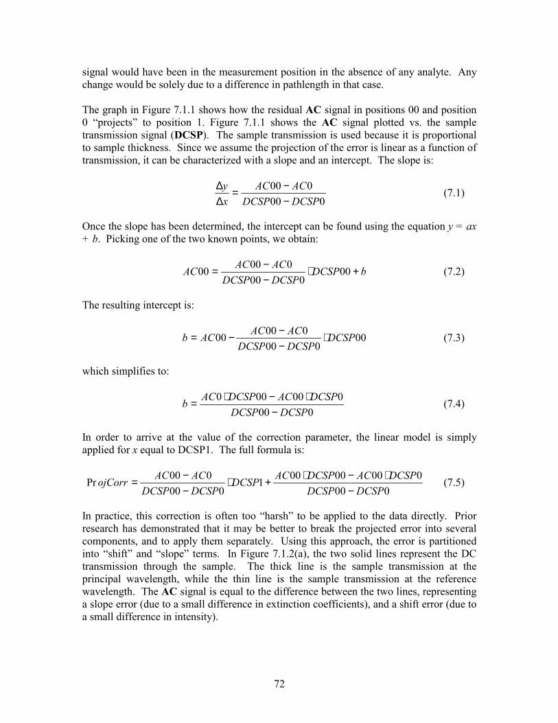
72
signal would have been in the measurement position in the absence of any analyte. Any change would be solely due to a difference in pathlength in that case. The graph in Figure 7.1.1 shows how the residual AC signal in positions 00 and position 0 “projects” to position 1. Figure 7.1.1 shows the AC signal plotted vs. the sample transmission signal (DCSP). The sample transmission is used because it is proportional to sample thickness. Since we assume the projection of the error is linear as a function of transmission, it can be characterized with a slope and an intercept. The slope is:
000000
DCSPDCSPACAC
xy
−−=
∆∆ (7.1)
Once the slope has been determined, the intercept can be found using the equation y = ax + b. Picking one of the two known points, we obtain:
bDCSPDCSPDCSPACACAC +⋅
−−= 00
00000000 (7.2)
The resulting intercept is:
00000
00000 DCSPDCSPDCSPACACACb ⋅
−−−= (7.3)
which simplifies to:
000000000
DCSPDCSPDCSPACDCSPACb
−⋅−⋅= (7.4)
In order to arrive at the value of the correction parameter, the linear model is simply applied for x equal to DCSP1. The full formula is:
000
00000001000
000PrDCSPDCSP
DCSPACDCSPACDCSPDCSPDCSPACACojCorr
−⋅−⋅+⋅
−−= (7.5)
In practice, this correction is often too “harsh” to be applied to the data directly. Prior research has demonstrated that it may be better to break the projected error into several components, and to apply them separately. Using this approach, the error is partitioned into “shift” and “slope” terms. In Figure 7.1.2(a), the two solid lines represent the DC transmission through the sample. The thick line is the sample transmission at the principal wavelength, while the thin line is the sample transmission at the reference wavelength. The AC signal is equal to the difference between the two lines, representing a slope error (due to a small difference in extinction coefficients), and a shift error (due to a small difference in intensity).

73
Figure 7.1.1: The residual AC signal in the 00 and 0 position is projected into the 1 position.
When partitioning the error into the slope and shift terms, a reference point is needed. The 00 position is chosen. The shift at this point is equal to AC00, which is proportional to the difference in intensity of the two phases of the light beam. Therefore, the shift error term is proportional to AC00. The remaining “rotation” of the AC signal (see Figure 7.1.2) is due to the slope error. If the slope error were zero, the AC signal at positions 00 and 0 would be the same. (In this case, the extinction coefficients for both wavelengths would be identical, and the only change over distance would be in intensity.) By extension, the slope error must therefore be proportional to the difference between AC00 and AC0, since this represents the rate of change of the intensity difference over thickness. A graphical representation of this phenomenon is shown in Figure 7.1.2. The preceding analysis showed that the calculated shift and slope terms are proportional to the error. The question remains as to how to find the proportionality constants. In terms of the shift error, we can assume that a relationship based on Beer’s Law holds. This would suggest that a logarithmic correction is required. In practice however, we are working over very small distances, and therefore we can approximate the curve to be linear in the region of interest. We therefore use a proportionality constant of DCSP1/DCSP00. This number approximates the transparency of the sample, or the attenuation over distance. Therefore, the final form of the shift error correction is
10000
DCSPDCSPAC ⋅ (7.6)
The slope error term also receives a correction factor of DCSP1/DCSP00, but an extra coefficient is added to account for the fact that the error changes with distance. Therefore, the constant should be approximately equal to the ratio between the balance distance and the measurement distance (usually about eight). It is often smaller than this
DCSP00 DCSP0 DCSP1 [Volts]
[Volts] AC00 AC0
AC1

74
in practice, generally having a value of two. The final form of the slope error term is then:
001)000(2
DCSPDCSPACAC ⋅−⋅ (7.7)
The overall projection correction formula is given by:
001))000(200(
DCSPDCSPACACAC ⋅−⋅− (7.8)
Figure 7.1.2: The residual AC signal after balancing must be partitioned into a shift term and a slope term. In the top part of the figure, the thicker line represents the transmitted intensity at the principal wavelength through the sample, while the reference intensity is the thinner line. In the bottom left figure, the shift term, which is proportional to AC00 has been extracted by constructing a line parallel to the principal intensity at the 00 position. In the bottom right figure, the slope term has been extracted by finding the “rotation” around the constructed line found while calculating the shift error. This “rotation” is proportional to the slope error.
7.1.2 Transparency Correction In the previous section, the slope and shift error terms were normalized by the transparency of the sample, which was represented by DCSP1/DCSP00. The bridge value itself should also be corrected for the sample transparency, as this will have an effect on the magnitude of AC. Again, a linear correction is used here rather than a
00 0 1
AC00
AC0
AC1
DC
Intensity
position
00 0 1
AC00 DC
Intensityposition 00 0 1
DC
Intensity
position
Shift ErrorSlope Error ∝ AC00-AC0

75
logarithmic correction due to the small distances involved in the measurement. The proportionality constant here is simple, and again it should be equal to the ratio between the measurement distance and the balance distance. Experience has shown that this constant has a value of approximately 5. The transparency correction is therefore:
0015
DCSPDCSP⋅ (7.9)
7.1.3 Temperature Correction It is well known that temperature affects the optical spectrum of a sample, drastically affecting the outcome of a measurement. While the design of the system includes measures to control temperature, it cannot be controlled tightly enough to prevent this effect. Fortunately, simple corrections can be applied here as well. The AC signal increases linearly with sample temperature. This has been verified through experimentation. Therefore, the appropriate correction is of the form:
AC1 –α⋅SAMPTEMP1 (7.10)
where α is the proportionality constant. This constant has been found experimentally to be approximately 0.004.
7.1.4 Reference Intensity Fluctuation Correction
Once the intensity-balancing portion of the reading is complete, the reference intensity (R_INT) should remain the same over the course of the measurement. Minor fluctuations do occur however, and they do have an effect on the measurement. A correction parameter can be found for this as well. Since the DC signals appearing at the auxiliary detector (AD) are immune to sample variations, they are solely affected by the R_INT variations. After the intensity balancing, the DC signals at the AD are DCIP00 and DCIR00.
After the measurement is complete, the measured signals are DCIP1 and DCIR1. The variation between DCIP1 and DCIP00, known as DDCIP1, represents drift in the intensity of the principal wavelength phase over the course of the measurement. Drift also occurs in the reference wavelength phase of the beam, and is represented by the difference between DCIR1 and DCIR00, known as DDCIR1. This drift includes effects from the principal wavelength of the beam as well as from drift in the reference intensity, since the R_INT voltage is a slave control.
We wish to find the variation that is only due to the changes in the R_INT voltage. The R_INT variation is actually proportional to the difference in drift (that is to say, it is the difference of the difference) between Sample Detector (SD) and the Auxiliary Detector (AD). (Recall that R_INT is a slave control to the Principal Intensity (P_INT)). Before the two drift values can be subtracted, they must be scaled. The AD gain is different from the SD gain. Since we are trying to correct the AC signal, which is derived from SD signals, we must normalize to this value. Therefore, the DCIP drift is scaled by a

76
factor known as DCRATP1, which has a value of DCSP1/DCIP1, while the DCIR drift is scaled by a factor known as DCRATR1, which has a value of DCSR1/DCIR1. The resulting factor, called CORR1 is therefore proportional to:
( ) ( )00111001
111 DCIRDCIR
DCIRDCSRDCIPDCIP
DCIPDCSPCORR −⋅−−⋅= (7.11)
A similar expression can be found for the 0 (wavelength balancing) position by replacing the 1 suffixes with 0’s. This expression is known as CORR0. Before this correction can be used, a final proportionality constant is required however. Since we are dealing with measurements on the DC channel, the extra gain in the AC channel over the DC channels is the appropriate correction value. This number is 35.
7.1.5 Putting It All Together – The Algorithm The correction factors discussed in the previous sections are subtracted from the Optical Bridge signal, AC1, and the resulting value is then normalized by DCSP1. A simple linear model is then applied (i.e. the number is multiplied by a sensitivity coefficient, and a shift term is added.) The sensitivity and shift terms are experimentally determined, but can be calculated from the absorbance of the analyte and the electrical gains in the system. The final equation is therefore:
( ) ( )
( )( )
shiftDCSP
SAMPTEMPACACACDCSPDCSP
DCIRDCIRDCIRDCSRDCIPDCIP
DCIPDCSPAC
ySensitivitConc
+
�
����
�
�
⋅−−−⋅−⋅−
���
� −⋅−−⋅⋅−
⋅=1
1004.05000200001
001(11001
11351
.
(7.12)
7.2 Multiple Linear Regression Approach In the past, analyte concentration levels have been obtained from Optical Bridge data using the simple linear model described in the previous section. The signal was normalized, certain correction parameters were applied, and finally a slope and intercept were used to arrive at the final concentration estimate. While this linear model has yielded good in-vivo results, it has shown limited applicability to recent in-vitro tests using a tissue simulator. We hypothesized that certain factors, temperature especially, have a detrimental effect on the quality of our in-vitro results, and therefore began to look for a more descriptive model. When the original model was applied to our data, the results were extremely poor. To start, the data was noisy. The standard deviation for repeated measurements of the same sample was generally over 50 mg/dl and significant drift was seen to occur in the measurements, sometimes as much as 100 to 200 mg/dl per hour. It became clear that a new algorithm was needed to obtain accurate urea results.

77
One solution to this problem would have been to take all of the available data from the instrument and apply a neural network or other type of data fitting algorithm to obtain a model for the desired output. This type of blind approach is very dangerous, and rarely takes into account the physical basis for variations in data. In addition, neural networks and other types of non-linear models do little to explain the variation in a system in a physical sense. Much of the processing involved in these algorithms is hidden from the user, in many cases preventing a true picture of the system from emerging. It is very easy to generate false correlations with this type of blind modeling. In order to develop a model that accurately represents the system in a predictable way, it is necessary to understand how the individual data items relate, (at least in an empirical sense), to each other and to the system as a whole. When modeling data, there are two possible approaches to take. The first approach assumes that all physical effects can be explained and modeled mathematically, and that by including them in the model, they can be compensated for. The linear model presently in use is an example of this approach. The second approach assumes that observed effects on the system can be explained heuristically, and mathematical information about them can be extracted by statistical methods. While we are able to derive a mathematical model for the ideal operation of this system (see §4.6.2), the presence of noise and uncontrollable variations like temperature induce some non-linear effects on the system that prevents the development of an analytical model. Therefore, the parameters will have to be selected from empirical knowledge of the system, and analysis of data, and new models will be developed using least-squares fitting techniques. When developing this algorithm, we had several performance goals in mind, representing major improvements over existing algorithms. (See Chapter 2). First, the algorithm needs to be robust enough to accurately predict dialysate urea concentration for any patient without the need for frequent recalibration. Second, measurements recorded with the existing algorithm require a tight set of operating parameters. The algorithm developed here must be valid for all patients and to any operating state of the instrument other than extreme failure (catastrophic failure of the instrument, such as loss of RF or light power). It is therefore necessary to understand and characterize how the instrument operates, and to then develop models based on this understanding, rather than blind applications of mathematical/statistical computing techniques. Developing a model based on this approach involves making a list of factors based on causative relationships that are hypothesized to produce variation in the data recorded by the instrument, and then attempting to fit the data to the desired output. This fitting is accomplished using a Multiple Linear Regression (MLR) analysis. (See §4.9) Here we discuss the evolution of our MLR algorithm and the pitfalls of applying this type of algorithm to our data, and how we avoided them.
7.3 MLR fitting concerns The first concern when using an MLR approach is to make sure that the problem is well-specified, and not over-fit. The predictive power of a model is poor when a large number

78
of variables are fitted to a small amount of data. In addition, if the range of the model data is small, it may not be possible to adequately predict the full range of the output variable when the model is applied. It is therefore important that the data be normally distributed and that an adequate amount of data is used to construct the model. Urea values in dialysate can be assumed to follow a normal distribution, since they are linearly related to blood urea concentration, which follows a normal distribution [79]. In many cases, the definition of “adequate amount” follows a rule of thumb rather than hard and fast numerical formulas. In general, data should outnumber model variables by a factor of at least three [77]. We will use no more than 16 MLR variables, so we need at least 48 tests. Our calibration set consists of 60 measurements that were derived from repeated measurements on three different samples. Because the sample data contains information about variation in the instrument that is unrelated to the sample, and because the number of modifying factors is large, the repeated measurements can be assumed to be independent [80]. The size of the data set thus exceeds the requirement that the number data points be greater than three times the number of variables [80]. In addition, several tests can be done using the ANOVA to check for significance of the model. The R2 value of the model is a good starting point for determining whether or not the chosen variables can be used to fit to the desired output. This value alone carries little weight however. The significance of the model can be determined using an F-test. The value of the F-test is related to the probability that the observed relationship between the observed value of the output and the model value occurred by chance [81]. This value can then be converted to a significance level by considering the degrees of freedom in the model. The F distribution is used to compare the variances of two sets of data. Here, the degrees of freedom are related to the ratio of regression variables to total data points. A second rule of thumb is that the value of the F distribution obtained from the regression should exceed the value of R2 by a factor of 10. (i.e. if R2 = 0.75, then F should have a value of at least 7.50. If these conditions are met, then the probability that the data set occurred by chance is low [82]. Arnold et al. [83] recently demonstrated that they were able to produce a phantom glucose calibration model using a multivariate model when the data was collected in a time dependent manner. This study used tissue simulators that contained no glucose, only water and bovine albumin in a phosphate buffer. First, the authors tried to predict the “glucose” level of the tissue simulator using a randomly assigned glucose concentration for each sample. They were unable to predict glucose concentration, with standard errors over 110 mg/dl and an R2 of 0.13. The samples were then reassigned a different glucose concentration that resembled one of three daily glucose profiles as reported in other studies. These glucose profiles were obtained by patients who were undergoing either an oral glucose tolerance test or injecting insulin. The authors were then able to predict the assigned glucose concentration, (standard error 24 to 66 mg/dl, R2 =0.54 to 0.84) even though there was no actual glucose in the sample. They concluded that an uncontrolled experimental parameter is responsible for the apparent good fit of the model. It was necessary to keep these results in mind when designing the experiment and interpreting the results of this multivariate approach.

79
Since we designed our experiments and were aware of these potential problems in applying the MLR algorithm, we can be confident that our algorithm will be able to produce predicted urea levels that are not correlated by chance to the actual urea concentration.
7.4 Choosing the Model Factors – The Evolution of the MLR Algorithm For each measurement, a large amount of data encompassing many variables is saved to a file. In total, 36 individual data items are saved for each measurement. With MLR, the objective is to determine which variables are the most important to the model. We expect that the signal will be strongly related to factors such as sample temperature and sample transmission. There are two possible reasons to discount a variable. First, the variable may be redundant if it is strongly correlated to one or more other variables in the data set. Second, the variable may not show a strong correlation to the resulting AC signal, and is therefore deemed to be unrelated to the urea concentration. In order to perform the task of parameter reduction in a systematic way, we evaluate the partial correlation of each variable with the others in a “correlation matrix”. The correlation matrix gives us an easy way of viewing the relative strength of relationships between variables. It is important not to completely rely on statistical correlation however. Inclusion of a particular factor in the model must “make sense” from our knowledge of how the Optical Bridge works. In order to develop a robust algorithm, we must combine the statistical data with our physical knowledge to arrive at a model that can accurately predict the sample urea content. The 36 variables that are saved to the file after each measurement are listed in Table 7.4.1. Variables that are used in the model are shown in bold type.
Table 7.4.1: List and description of data items obtained from each measurement. (Bolded variables are used in MLR model).
PRI_WL Principal wavelength REF_WL Reference wavelength PRI_INT Intensity of principal wavelength phase of the light beam OFFSET Used to set difference between P_INT and R_INT AC00 Differential sample transmission signal after intensity balancing AC0 Differential sample transmission signal after wavelength balancing AC1 Differential sample transmission signal with spent dialysate in optical path DCSP00 Sample transmission at principal wavelength after intensity balancing DCSP0 Sample transmission at principal wavelength after wavelength balancing DCSP1 Sample transmission at principal wavelength with spent dialysate in optical path DCSR00 Sample transmission at reference wavelength after intensity balancing DCSR0 Sample transmission at reference wavelength after wavelength balancing DCSR1 Sample transmission at reference wavelength with spent dialysate in optical path R_INT00 Intensity of reference wavelength beam phase after intensity balancing R_INT0 Intensity of reference wavelength beam phase after wavelength balancing R_INT1 Intensity of reference wavelength beam phase with spent dialysate in optical path

80
DCIP00 Incident power at AD at principal wavelength after intensity balancing DCIP0 Incident power at AD at principal wavelength after wavelength balancing DCIP1 Incident power at AD at principal wavelength with spent dialysate in optical path DCIR00 Incident power at AD at reference wavelength after intensity balancing DCIR0 Incident power at AD at reference wavelength after wavelength balancing DCIR1 Incident power at AD at reference wavelength with spent dialysate in optical path SAMPLET00 Temperature of the sample after intensity balancing SAMPLET0 Temperature of the sample after wavelength balancing SAMPLET1 Temperature of the sample with spent dialysate in optical path DETT00 Temperature of the SD after intensity balancing DETT0 Temperature of the SD after wavelength balancing DET1 Temperature of the SD with spent dialysate in optical path DIS00 Sample thickness after intensity balancing DIS0 Sample thickness after wavelength balancing DIS1 Sample thickness with spent dialysate in optical path K Ratio of DCSP1 to DCSP00 ACC1 AC1 corrected for residual balance signals DELK00 ACC1/DCSP00 DELK0 ACC1/DCSP0 DELK1 ACC1/DCSP1 In general, we attempted to find an optimal set of parameters that explain both the variation in the data due to changes in urea content and instrumental fluctuations. We needed a method to reduce the number of variables in the analysis from 36 to something more reasonable. Sets of variables that contained the same basic information (redundant variables) were the first to be eliminated. Redundant variables were considered to be those that were more than 99% correlated with another variable in the set. The correlation data was derived from the results of the baseline (water only) study data. The relationships were analyzed using a correlation matrix, which is a tool used to graphically represent the degree to which a set of variables relate to each other (See §8.1). Physically, these variables generally have direct relationships with each other as a consequence of hardware design. Only one variable of any related set was included. The following variables were eliminated on the basis of redundancy:
��DCSP00, DCSP0, DCSP1, DCSR00, DCSR0, DCSR1, DCIP00, DCIP0, DCIP0, DCIP1, DCIR00, DCIR0, DCIR1, R_INT00, R_INT0, R_INT1 – all of these are strongly correlated with OFFSET;
��DIS00, DIS0 – both of these are directly related to DIS1; ��SAMPLET0 – strongly related to SAMPLET00.
After this first step, 17 variables remain. The detector temperature variables (DETT00, DETT0, and DETT1) in the baseline study correlation matrix showed little or no relationship to the signal variations. They can be omitted, reducing the count to 14. Next, there are certain variables that are held constant or rarely change. These are PRI_WL and P_INT. This step reduces the variable count to 12.

81
It is not only necessary to determine which variables can be excluded, but also to determine which variables must be included. To do this, we must determine which of the remaining variables have the strongest power in estimating sample urea content. These may be variables that relate to urea information, or to variations in the instrument, or both. This involved analysis of both the baseline studies and preliminary urea/water studies. The results of these measurements were analyzed for significant relationships by the development of a correlation matrix to determine how strongly each variable relates to the others. Most importantly, we were interested in how each of the remaining signals correlated to the measured signal, AC1. Results of these preliminary tests had shown that the most significant non-urea related variations in the data were caused by:
a) sample temperature b) fluctuations in transparency of the sample c) residual signal after balancing
The preliminary tests also showed that the most significant variations in the data caused by urea were related to: AC1, ACC1, DELK00, DELK0, and DELK1. It was therefore necessary to include variables that would compensate for these effects. The possibilities are:
a) sample temperature variations: SAMPLET0, SAMPLET1, OFFSET, REF_WL. The offset and reference wavelength data are indirectly related to temperature, because the spectrum of the sample shifts as temperature changes. Therefore, the values of these two items can be useful in predicting temperature shifts.
b) Sample transparency: K, DIS1. The transmission data that results from the measurement must be normalized for sample thickness and how well the sample transmits light. K is related to the extinction coefficient at the principal wavelength, and DIS1 is an indication of the thickness of the sample.
c) Residual signals: AC00, AC0. These signals indicate how well the system was able to balance out the background sample.
In order to select the optimal set of parameters for the algorithm from this sub-set, several regressions were performed on the remaining variables, bearing in mind the results of the baseline studies. First, each of the variables that were observed to correlate with urea concentration (AC00, AC0, ACC1, DELK00, DELK0, and DELK1) was included. None was significantly correlated with any other variable enough to warrant exclusion. AC00, AC0, and ACC1 are un-normalized differential transmission signals. AC00 is the residual signal in the thinnest sample position after intensity balancing. AC0 is the residual signal in the middle sample position after wavelength balancing. These two signals are therefore included in the algorithm because they form a starting basis for the rest of the measurement. ACC1 is the differential transmission signal in the thickest sample position, after the urea-laden dialysate has entered the path.

82
Using Equation 4.19, we know that the analyte signal should be proportional to the value of ∆k. The combination of temperature and geometry-related variations on the data obscures this relationship, and possibly introduces some non-linear effects. DELK00 is normalized by the starting thickness and corrected for the transparency of the sample and residual signal after balancing. DELK0 is a similar parameter, but its normalization is by the middle sample thickness, while DELK1 is normalized by the final sample thickness. Inclusion of all three parameters gives the algorithm a truer picture of how the transmission of the sample changes with sample and thickness composition. Next we need to determine which of the temperature related factors to include. Here again, we decided that all factors are important to the analysis, because they each provide different information. REF_WL is included as a measure of the temperature stability at the actual measurement wavelength. As the wavelength shifts, the temperature sensitivity changes. This is because the reference wavelength is located on a steep slope of the water peak, resulting in large changes in the transmission signal. The slope also changes as a function of temperature. The two sample temperatures SAMPLET0 and SAMPLET1 are both included because they give not only a measure of what the sample temperature is, but also a measure of how fast it is changing through the course of the measurement. Finally, OFFSET is included because it gives a measure of how the AC signal is drifting as a function of temperature. This phenomenon is explained more fully in §8.3.1. Both variables relating to sample transparency were included as well. The extinction coefficient of the measurement and the sample thickness are both important to the goal of establishing a universal calibration for all patients and all instrumental variations. Therefore the DIS1 and K variables are also included. After analyzing the correlation matrices for the baseline and urea studies, the following twelve variables and functions of variables were selected for inclusion in the model: REF_WL, OFFSET, SAMPLET0, SAMPLET1, DIS1, K, AC00, AC0, ACC1, DELK00, DELK0, and DELK1. These variables have been found to be the most significant to the overall result. Once the factors for the algorithm had been identified, the next task was to determine a “weight” for each variable according to the regression equation. This was done by giving the algorithm a set of training data consisting of several measurements repeated on the same sample. In this way, data related to both instrumental variations and urea level variations was presented to the algorithm. Using Microsoft Excel, we then performed a linear fit on the data to obtain the weight for each variable in the algorithm. Once this was accomplished, we needed to determine if each variable was actually significant to the algorithm. The algorithm was then used to predict the urea content of a number of other samples recorded on different days and under different conditions. The results of this process are described in Chapter 8. We were able to conclude that all variables are significant and provide a useful contribution to the algorithm, and that the algorithm was able to accurately predict sample urea content for all tested samples.

83
The resulting algorithm is therefore: ⋅=
kkk xdlmgUrea β)/( (7.13)
The weights (βk) of each variable (xk) in the algorithm are given in Table 7.4.2.
Table 7.4.2: Weighting coefficients for the MLR algorithm.
k Variable Name (xk) Coefficients (βk)0 Intercept -3793.048861 1 REF_WL 2.738386369 2 OFFSET 11.78231559 3 SAMPLET0 -15.08450145 4 SAMPLET1 8.278386882 5 DIS1 21.1473092 6 K 17.11947157 7 AC00 8.097130604 8 AC0 20.2117165 9 ACC1 266.3492255 10 DELK00 -40175.72805 11 DELK0 39278.75765 12 DELK1 -5.857607611
7.5 Dialysis Efficiency Monitoring Algorithm Once the estimate of urea level has been obtained using the algorithm described in the previous section, it is possible to arrive at a measure of dialysis efficiency. This measure of efficiency is related to the total urea removed during the dialysis session, and is therefore a simple integration. Due to the fact that the measurement is semi-continuous, a Riemann sum type of approximation can be used: Utot = ∆⋅= ttUUtot )( , where U(t) is the estimated urea concentration and ∆t is the time interval between samples. The sample urea content can also be used to estimate more traditional dialysis efficiency parameters such as kT/V. kT/V is related to the slope of the dialysate urea curve, as shown by Garred et al. [25]. kT/V can be expressed as:
hr
dry
D
TBW
BWTtC
VkT
01786.01
3)(ln
−
∆+∂
∂−
= (7.14)
The second term in Equation 7.14 relating to changes in body water is required to correct for changes in the urea distribution volume. This does not require any extra measurement, as these parameters are measured for all dialysis patients to determine the

84
required amount of fluid lost. Use of this formula can provide a projection of the value of kT/V that will be obtained during the session at an early time in the process, allowing the physician to change the patient’s treatment course if goals will not be met. In general, the dialysis session is considered accurate if kT/V is above 1. See §4.2.6 for a discussion of kT/V. Now that time dependent information concerning the urea content of the dialysate is available, future research may lead to the development of more efficiency parameters related to this measurement.

85
8 EXPERIMENTAL RESULTS The experimental portion of this research consisted of several stages: • = Preliminary studies measuring urea in water using the first generation prototype; • = Preliminary studies measuring pure water and urea in water using the NIV prototype; • = Analysis of the measured data, modeling, and extraction of urea estimation
parameters; • = Development of an algorithm based on multiple linear regression for urea estimation
and dialysis efficiency monitoring; and, • = Performance testing of the urea estimation algorithm with hemodialysis patient
studies. In this chapter, a summary of all experiments is presented first. Then, results from each set of measurements are presented and some specific characteristics of the measurements are described. The results of the algorithm development process are then shown. Finally, the results of applying this algorithm to samples of patient dialysate are presented.
8.1 Summary of Experiments During the course of three years, over 2000 optical measurements were performed using three different prototypes. Approximately 1000 of these measurements were performed with the prototype instrument used in this research to measure urea. Almost 600 measurements were performed using the NIV prototype to measure the effects of temperature on the optical measurement in the absence or urea. 50 measurements were done to obtain data about the system variability in the absence of urea. 160 measurements were performed on samples of urea in water using the NIV prototype. Finally, 154 measurements were performed on samples of spent dialysis fluid using a new prototype of the NIV system. The results of the studies using the prototype developed for this research are extremely poor. They will be described in the next section. Subsequent sections will detail the results of testing using the NIV prototypes. At first, results with these instruments were poor as well. However, after the development of the new algorithm, the results were greatly improved, and shown potential for clinical success. The final set of measurements recorded with the newest NIV system are extremely good, and show accuracy near that of standard reagent/electrode based instruments.
Table 8.1.1 is a record of the studies performed during the course of this research. It indicates the type of study, the instrument used to obtain the data, the algorithm used to process the data, the number of measurements recorded, and whether or not the study was successful. A CD-ROM with all of the recorded data is available from WPI – Biomedical Engineering Department Library.

86
Table 8.1.1 : Overview of the performed experiments and measurements.
Experiment Description
Prototype Algorithm Number Results
Urea in water Dissertation 1 1000 not successful Temperature NIV1 N/A (training data) 600 successful Baseline NIV1 N/A (training data) 50 successful Urea in water NIV1 1 160 not successful Urea in water NIV1 2 160 successful Spent dialysate NIV2 1 154 not successful Spent dialysate NIV2 2 154 successful
8.2 Results of Proof of Principle Studies As has been stated before, the results of the preliminary studies using the prototype developed for this research were very poor. Two independent sets of measurements were done. For the first, the temperature of the instrument and sample was allowed to vary freely. Figure 8.2.1 shows the results for this test. No sensitivity to urea is seen, and in reality the calibration graph is merely an average of the actual urea concentrations used in this study.
Figure 8.2.1: Estimated vs. Actual Urea for the dissertation prototype. Actual urea content was determined by weight (accurate to 0.1 mg) when samples were prepared. Temperature was allowed to vary freely. The graph shows that the correlation between the two measurements is almost non-existent (R2 = 0.0012). The standard error for this measurement series was over 500 mg/dl.
0.7900.7950.8000.8050.8100.8150.8200.8250.8300.8350.840
0.0 0.5 1.0 1.5 2.0
Actual urea [g/dl]
Estim
ated
ure
a [g
/dl]

87
A second study was performed after adding better temperature control to the measurement. The temperature variation was now kept to within ±1°C. After this modification, some dependence on the actual urea level was seen. As seen in Figure 8.2.2, the R2 value has improved to 0.94, but the system still had errors of over 100 mg/dl that could not be compensated for. In addition, the system had noise levels in hardware of well over 5 mV, which translated to approximately 25 mg/dl. The remaining error was attributed to temperature variations, and sample thickness variations. The sample thickness variations were thought to cause air bubbles and other types of sampling effects that degraded measurement accuracy. Even if these could be sufficiently modeled, the hardware noise alone would prevent adequate measurement accuracy. At this point, the decision was made to perform the rest of the studies with the NIV prototype.
Figure 8.2.2: Estimated vs. Actual Urea, dissertation prototype. Actual urea content was determined by weight (accurate to 0.1 mg) when samples were prepared. For this experiment, temperature variations were controlled to within ±±±± 1°°°° C. Standard error is still over 100 mg/dl. Approximately ¼ of the measurements were rejected for instrumental variations.
Despite the apparently poor results of these preliminary studies, important information about the effects of uncontrolled temperature and position variation on the data came to light. Compounding the problem was that the prototype could not reliable measure either sample temperature or sample thickness due to design considerations. For this reason, it is difficult to gain a true picture of the exact variation due to these factors. The results of testing with the NIV instrument were able to provide this information, however, which is described in the following sections.
8.3 Baseline (no urea) studies One of the most important results of this research is a set of baseline data. The baseline studies were performed exclusively with the NIV prototype instrument, since it was deemed to be the more accurate and stable of the two. This baseline data was used to
0.00.20.40.60.81.01.21.41.6
0 0.5 1 1.5Actual urea [g/dl]
Estim
ated
ure
a [g
/dl]

88
show relationships between different parameters and variables in the measurements. This data was then used to establish factors that were used in the development of the algorithm. One of the first steps in this procedure was to determine the extent to which certain variables correlate with each other. This is useful for several reasons. First, it may reduce the number of variables that must be used to characterize the system by pointing out which variables depend strongly on the others. For example, the R_INT signals and the DCIR would be expected to correlate strongly, and it would be unnecessary to include both of them as part of an algorithm. Second, it can suggest possible sources of error. For example, if the AC signal were found to depend strongly on temperature, a correction could be applied. Since there is a large amount of data, (approximately 36 variables), finding these relationships can be somewhat tedious. In an attempt to simplify the task, a graphical approach was taken. A “correlation matrix” was developed in Microsoft Excel as a starting point for determining which variables where strongly related. This correlation matrix was then plotted as a contour map in order to ease the task of identifying strong correlations. Once regions of high correlation values were identified, a list of factors to use in developing the algorithm was made. Figure 8.3.1 shows this contour plot. Areas of high correlation are shown in red and yellow. Areas of high negative correlation are shown in gray and black. Note that this graph is symmetrical about the diagonal. Any correlation over ±0.50 was deemed to be of interest. If no position (i.e. 00, 0, or 1) is given, then the relationship held true over all positions. (In other words, R_INT includes R_INT00, R_INT0, and R_INT1, for example). These groupings are listed in Table 8.3.1. These relationships will be explored in more detail in this section. (Basic definitions can be found in Table 5.2.1 and Table 7.4.1). Parameters such as K, ACC1, and DELK1 are not listed in the table because they are calculated, rather than measured. The overall signal value (DELK1) is listed in the table however because it may help to illustrate how several factors that do not correlate significantly to any of the raw data may combine to affect the calculated concentration value. In other words, it can lend validity to some of the correction factors discussed in §7.1, and possibly suggest new ones as well. This correlation matrix shown in Figure 8.3.1 was also used as a starting point for statistically optimized variable selection for the MLR algorithm, along with the results of the urea in water studies described in §8.4 and our knowledge of how this system works.

89
Figure 8.3.1: Plot of the correlation matrix for a baseline study. Red and yellow indicate strong positive correlations, while gray and black indicate strong negative correlations.
Table 8.3.1: Groupings of variables showing possible dependencies. The strength of the relationship between the variables in gray and the listed parameters is given by the correlation coefficient.
Strong Correlations (± 0.75 to 1.0) Correlation Coeff. Offset sample temperature -0.944 to -0.955 all DC and R_INT Signals -0.787 to -0.984 AC00 AC0 0.914 DC signals (DCSP, DCSR, DCIP, DCIR) All other DC signals 0.753 to 0.998 R_INT signals 0.753 to 0.995 sample temperature 0.752 to 0.973 Sample thickness DCSP 0.809 to 0.856 DCSR 0.805 to 0.853
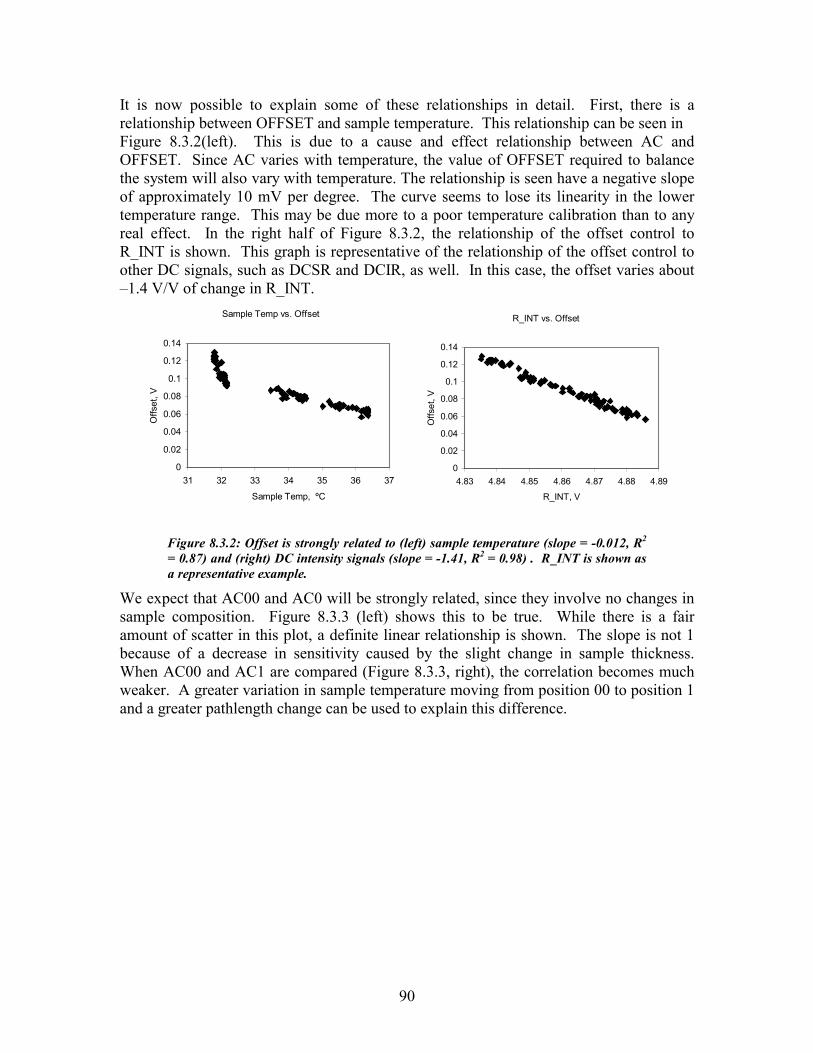
90
It is now possible to explain some of these relationships in detail. First, there is a relationship between OFFSET and sample temperature. This relationship can be seen in Figure 8.3.2(left). This is due to a cause and effect relationship between AC and OFFSET. Since AC varies with temperature, the value of OFFSET required to balance the system will also vary with temperature. The relationship is seen have a negative slope of approximately 10 mV per degree. The curve seems to lose its linearity in the lower temperature range. This may be due more to a poor temperature calibration than to any real effect. In the right half of Figure 8.3.2, the relationship of the offset control to R_INT is shown. This graph is representative of the relationship of the offset control to other DC signals, such as DCSR and DCIR, as well. In this case, the offset varies about –1.4 V/V of change in R_INT.
Sample Temp vs. Offset
0
0.02
0.04
0.06
0.08
0.1
0.12
0.14
31 32 33 34 35 36 37
Sample Temp, ºC
Offs
et, V
R_INT vs. Offset
0
0.02
0.04
0.06
0.08
0.1
0.12
0.14
4.83 4.84 4.85 4.86 4.87 4.88 4.89
R_INT, V
Offs
et, V
Figure 8.3.2: Offset is strongly related to (left) sample temperature (slope = -0.012, R2 = 0.87) and (right) DC intensity signals (slope = -1.41, R2 = 0.98) . R_INT is shown as a representative example.
We expect that AC00 and AC0 will be strongly related, since they involve no changes in sample composition. Figure 8.3.3 (left) shows this to be true. While there is a fair amount of scatter in this plot, a definite linear relationship is shown. The slope is not 1 because of a decrease in sensitivity caused by the slight change in sample thickness. When AC00 and AC1 are compared (Figure 8.3.3, right), the correlation becomes much weaker. A greater variation in sample temperature moving from position 00 to position 1 and a greater pathlength change can be used to explain this difference.

91
AC00 vs. AC1
-1.2
-1
-0.8
-0.6
-0.4
-0.2
0-0.6 -0.5 -0.4 -0.3 -0.2 -0.1 0
AC00, V
AC1,
V
AC00 vs. AC0
-0.7
-0.6
-0.5
-0.4
-0.3
-0.2
-0.1
0-0.6 -0.5 -0.4 -0.3 -0.2 -0.1 0
AC00, V
AC0,
V
Figure 8.3.3: AC00 and AC0 are strongly correlated (slope = 0.89, R2 = 0.72) with each other (left). AC00 and AC1 do not have a strong relationship(slope = 0.55, R2 = 0.08) (right).
A final strong relationship can be seen between the sample thickness and the DC transmission parameters such as DCSP and DCSR. A representative relationship is shown in Figure 8.3.4 between sample thickness and DCSP. DCSP changes by about 117 mV per mm of change in sample thickness.
DCSP00 vs. DIS00
0
0.5
1
1.5
2
4.2 4.7 5.2 5.7 6.2
DIS00, mm
DC
SP00
, V
Figure 8.3.4: Sample thickness is strongly related (slope = 0.12, R2 = 0.47) to DC values at the sample detector. DCSP is shown as a representative example.
Many of these relationships that are seen to exist from analyzing Figure 8.3.1 can be explained from direct hardware principles. Direct hardware relationships like DCSR vs. R_INT are not of interest here, but some of the other less direct relationships presented in this section are of interest. The most important of these variations is that of temperature. A separate study involving over 570 optical spectra was performed to characterize the temperature response of the system. In addition, the 50 baseline measurements were analyzed for temperature dependence of data. The following sections present an explanation of some of the results of these studies.
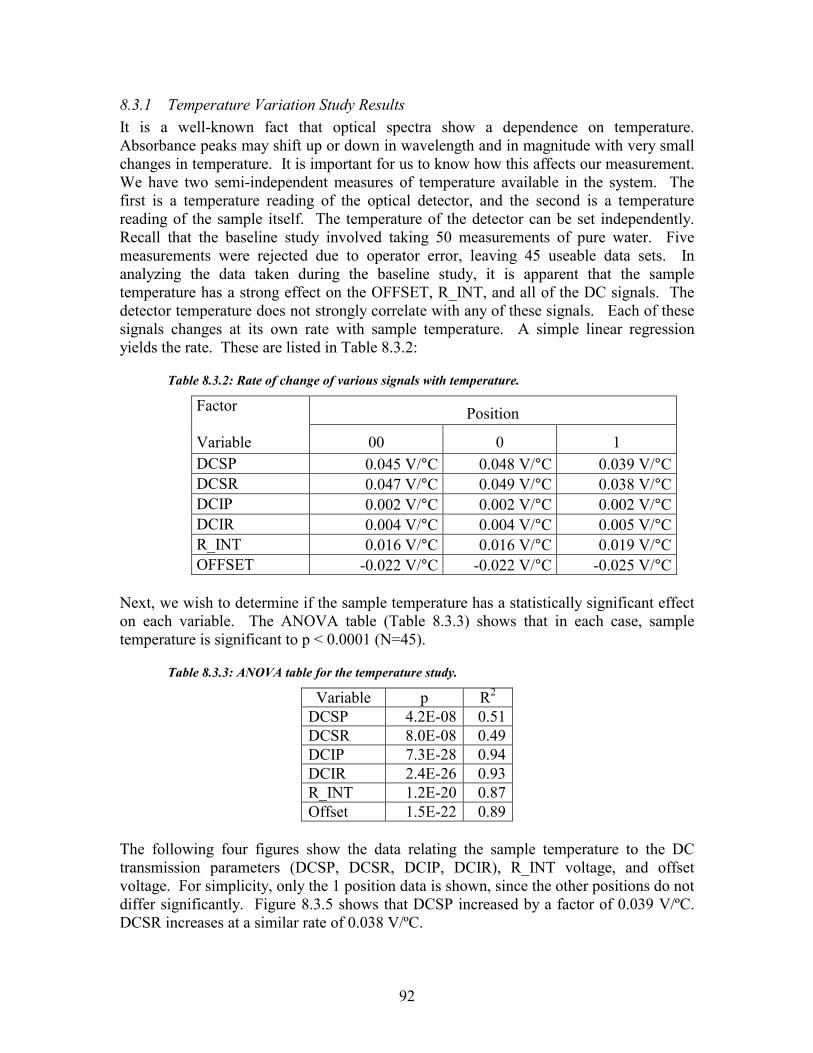
92
8.3.1 Temperature Variation Study Results It is a well-known fact that optical spectra show a dependence on temperature. Absorbance peaks may shift up or down in wavelength and in magnitude with very small changes in temperature. It is important for us to know how this affects our measurement. We have two semi-independent measures of temperature available in the system. The first is a temperature reading of the optical detector, and the second is a temperature reading of the sample itself. The temperature of the detector can be set independently. Recall that the baseline study involved taking 50 measurements of pure water. Five measurements were rejected due to operator error, leaving 45 useable data sets. In analyzing the data taken during the baseline study, it is apparent that the sample temperature has a strong effect on the OFFSET, R_INT, and all of the DC signals. The detector temperature does not strongly correlate with any of these signals. Each of these signals changes at its own rate with sample temperature. A simple linear regression yields the rate. These are listed in Table 8.3.2:
Table 8.3.2: Rate of change of various signals with temperature.
Position Factor Variable 00 0 1 DCSP 0.045 V/°C 0.048 V/°C 0.039 V/°CDCSR 0.047 V/°C 0.049 V/°C 0.038 V/°CDCIP 0.002 V/°C 0.002 V/°C 0.002 V/°CDCIR 0.004 V/°C 0.004 V/°C 0.005 V/°CR_INT 0.016 V/°C 0.016 V/°C 0.019 V/°COFFSET -0.022 V/°C -0.022 V/°C -0.025 V/°C
Next, we wish to determine if the sample temperature has a statistically significant effect on each variable. The ANOVA table (Table 8.3.3) shows that in each case, sample temperature is significant to p < 0.0001 (N=45).
Table 8.3.3: ANOVA table for the temperature study.
Variable p R2 DCSP 4.2E-08 0.51DCSR 8.0E-08 0.49 DCIP 7.3E-28 0.94DCIR 2.4E-26 0.93R_INT 1.2E-20 0.87Offset 1.5E-22 0.89
The following four figures show the data relating the sample temperature to the DC transmission parameters (DCSP, DCSR, DCIP, DCIR), R_INT voltage, and offset voltage. For simplicity, only the 1 position data is shown, since the other positions do not differ significantly. Figure 8.3.5 shows that DCSP increased by a factor of 0.039 V/ºC. DCSR increases at a similar rate of 0.038 V/ºC.

93
Sample Temperature vs. DCSP and DCSR
0.630.640.650.660.670.680.690.7
0.71
28 28.5 29 29.5 30 30.5
Sample Temp, ºC
DC
SP, V
0.610.620.630.640.650.660.670.680.690.7
DC
SR, V
Figure 8.3.5: The light transmission through the sample is an increasing function of temperature (DCSP vs Temperature: slope = 0.04, R2 = 0.49, DCSR vs. Temperature: slope = 0.04, R2 = 0.51). DCSP is plotted with diamonds, DCSR is plotted with squares.
It is important to note that the rate of change of signals with respect to temperature is not the same for the SD and the AD. The increase in the factor between DCSP and DCIP is approximately 17.7, which is far greater than the actual gain of 6 between the SD and the AD. See Figure 8.3.6. This suggests that the temperature effects arise mainly from the physical properties of the sample, rather than the properties of the instrument. The data also shows that the temperature effects are more significant at the reference wavelength for the AD. The increased sensitivity of the reference wavelength is to be expected, since it lies on the edge of a strong water absorbance peak. The slope of the absorbance curve is steeper there, leading to a greater change with temperature. This data suggests that any correction based on temperature may be related to the slope of the spectrum around the reference wavelength. The fact that the SD did not show this dependency on wavelength can be explained by the fact that the data was recorded after the balancing phase of a measurement, causing the system to adjust to the spectral changes in the sample.

94
Sample Temperature vs. DCIP and DCIR
0.16150.162
0.16250.163
0.16350.164
0.16450.165
0.16550.166
28 28.5 29 29.5 30 30.5
Sample Temperature, ºC
DC
IP, V
0.15
0.152
0.154
0.156
0.158
0.16
DC
IR, V
Figure 8.3.6: The sensitivity of the AD (DCIP vs. Temperature: slope = 0.002, R2 = 0.94, DCIR vs. Temperature: slope = 0.005, R2 = 0.93) to increasing sample temperature is an order of magnitude lower than that of the SD and shows a dependence on wavelength. DCIP is plotted with diamonds, DCIR is plotted with squares.
While the R_INT and OFFSET voltages both appear to respond to temperature, in fact, neither is directly affected. Instead, it is the AC signal that is affected. As the temperature rises, so does the AC signal. This causes the offset required to balance the system during measurement to decrease. It changes with a slope of –0.025 V/ºC. As the OFFSET decreases, the R_INT voltage increases with a slope of 0.019 V/ºC. The only question is whether or not the R_INT is independently temperature sensitive. It does not appear so, as the ratio of temperature sensitivity factors is –1.35, which is very close to the OFFSET/R_INT gain of –1.30. The plots of R_INT voltage and OFFSET voltage vs. Sample Temperature during measurement are shown in Figure 8.3.7 and Figure 8.3.8.
Sample Temperature vs. R_INT
4.854.855
4.864.865
4.874.875
4.884.885
4.89
28 28.5 29 29.5 30 30.5
Sample Temp, ºC
R_I
NT,
V
Figure 8.3.7: The R_INT voltage also increases linearly with sample temperature (slope = 0.019, R2 = 0.87) .

95
Sample Temperature vs. Offset
0
0.02
0.04
0.06
0.08
0.1
0.12
28 28.5 29 29.5 30 30.5
Sample Temp, ºC
Off
set,
V
Figure 8.3.8: The offset voltage that was required to balance the bridge decreased as a function of sample temperature (slope = -.025, R2 = 0.89).
Since we have determined that the fluctuations in the Offset and R_INT voltages are in fact induced by changes in the AC signal, the question remains of what is the true sensitivity of the instrument to temperature. Since any changes are balanced out during the measurement, this sensitivity must be measured separately. The water-filled tissue simulator was tested at three different wavelength pairs: 1600.0/1379.6, 1620.0/1379.6, 1640.0/1379.6. These wavelengths were selected because they could all be balanced with the same reference wavelength, thus reducing the number of variables. We were not able to find similar pairs in the range of urea measurements. The system was initially balanced manually, and then the system temperature was adjusted. The system data was then recorded every 20 seconds. The temperature was adjusted both up and down to eliminate variations due to drift. The results of this test are shown in Table 8.3.4. The AC signal tracked the temperature variations very closely. The results of this study are shown in Figure 8.3.9. The larger difference in the first part of the data can be accounted for by a poor initial balanced condition.

96
Sample Temperature with AC
31.5
32
32.5
33
33.5
34
34.5
35
35.5
36
36.5
37
Sam
ple
Tem
p (C
)
-0.5
0
0.5
1
1.5
2
2.5
AC
(V)
Sample Temp AC
Figure 8.3.9: Response of the signal to temperature variations. The three groupings represent data taken at 1600 (left data group), 1620 (middle data group), and 1640 nm (right data group).
Using this data, we can attempt to find a rate of change of the AC signal with temperature. A simple linear regression is used here as well. Table 8.3.4 shows that the slope does vary with wavelength, and that temperature is has a statistically significant effect at all of the test wavelengths to p < 0.0001. The slope effect is on the order of 400 mV/ºC, which is very significant considering the magnitude of changes that are generally induced by the presence of an analyte in the signal. (On average, this change is a few tens of millivolts at physiological concentrations. The results of this testing are shown in Figure 8.3.10
Table 8.3.4: The rate of change of AC vs. temperature depends on wavelength.
Wavelength Slope Factor p value N 1600 0.43 3.1 E-119 190 1620 0.42 1.9 E-198 190 1640 0.49 2.1 E-208 191

97
AC vs. Sample Temp - Linear Fit
-0.5
0
0.5
1
1.5
2
2.5
31 32 33 34 35 36 37Sample Temp, ºC
AC, V
Figure 8.3.10: Variation of the AC signal with sample temperature at three wavelengths. At 1620 nm (squares), the sensitivity is 0.42V/ºC (R2 = 0.99). At 1640 nm (triangles), the sensitivity is 0.49 V/ºC (R2 = 0.99)
In analyzing the results of the baseline study, we have gained significant understanding in the effects of temperature and other system variations such as sample thickness on the data. It shows that sample temperature must certainly be included in any kind of MLR algorithm, as well as the offset. This analysis has also allowed us to determine which parameters are redundant in the analysis and can therefore be omitted in favor of others in the MLR algorithm. The extraction of the remaining parameters will be accomplished by analyzing the results of the urea in water studies.
8.4 Results of the Urea Level Estimation Studies: Urea in Water Studies This section explains the results of the urea in water measurements that were performed using the NIV prototype. First, the results of the measurements using algorithm 1 will be presented. As was stated in the introduction to this chapter, this algorithm could not be used to successfully estimate the urea level of the samples. The remainder of this section will then show how algorithm 2 evolved from the results of these studies. We will show how successfully this algorithm is able to estimate the sample urea concentration when applied to the data. Finally, we will show that the results indicate that the algorithm is able to fulfill the performance goals laid out in Chapter 2.
8.4.1 Results of application of Algorithm 1 It is not possible to use algorithm 1 to estimate urea concentration using this method. The results of this study when algorithm 1 is applied to the data are shown in Figure 8.4.1. The calibration line shows no sensitivity to the presence of urea.

98
Estimated vs. Actual Urea
020406080
100120140160
0 50 100 150 200 250
Actual Urea, [mg/dl]Es
timat
ed U
rea,
[mg/
dl]
Figure 8.4.1: Urea Estimation Calibration curve for algorithm 1. Actual urea content was determined by weight (accurate to 0.1 mg) when samples were prepared. The algorithm shows no predictive power for this study (R2 = 0.04).
We have not yet provided an explanation from the data as to why the mathematical model developed in §4.6.2 cannot be used here. We have hypothesized that temperature and sample thickness variations prevent sufficient measurement stability. The graph in Figure 8.4.2 shows a plot of 40 measurements that were recorded from the same sample. In addition to a fairly significant noise level, there is a large drift happening in the AC1 plot. The noise in AC1 appears to be directly related to the noise in AC00 and AC0. These two factors are therefore useful in explaining variation in AC1, and will be included as parameters in the development of algorithm 2.
AC signals
-0.5
-0.4
-0.3
-0.2
-0.1
0
0.1
0.2
AC
, V
AC00 AC0 AC1
Figure 8.4.2: This graph shows a series of 40 measurements taken over a 4 hour period using the same sample. The figure shows that significant drift occurs in the baseline level of AC1 over the course of the measurement series.

99
The inclusion of DELK00, DELK0, and DELK1 in the model is based on similar reasoning. These are really just normalized versions of AC00, AC0, and AC1. The graphs of these variables look very similar to that of Figure 8.4.2. The graph in Figure 8.4.3 demonstrates that the signal AC1 does indeed vary strongly with sample temperature. The right hand plot in the figure shows a strong linear relationship with the sample temperature. Several outliers can be seen in this plot that are the result of other types of variations. The left hand side of the figure shows the time course of both the temperature measurement and AC1. Visual inspection of the course indicates that the drift in AC1 is strongly related to the sample temperature.
-0.5
-0.4
-0.3
-0.2
-0.1
0
0.1
AC
1, V
32.8
33
33.2
33.4
33.6
33.8
34
34.2
Sam
ple
Tem
p, ºC
AC1 SAMPLET1
Sample Temp vs. AC1
-0.5
-0.4
-0.3
-0.2
-0.1
0
0.1
33.0 33.5 34.0 34.5Sample Temp, ºC
AC
1, V
Figure 8.4.3: These two figures demonstrate the variation of AC1 with sample temperature. The right hand side of the figure shows a scatter plot of temperature vs. AC1 (slope = 0.39, R2 = 0.60), while the left hand side shows the time course of both variables.
Two other system variables also show this drift characteristic during repeated measurements of the same sample: OFFSET and REF_WL. Since the value of these parameters are set by balancing, in order to minimize AC00 and AC0, it makes sense that the drift would be seen in the offset and reference wavelength, rather than in AC00 and AC0. The four graphs pictured in Figure 8.4.4 show how the drift in AC1 is mimicked by drift in OFFSET and REF_WL. So the results of this study indicate that OFFSET, REF_WL, and SAMPLE_TEMP are all useful parameters in explaining drift that occurs in the optical signal. Further characterization of the data is required to sufficiently explain rest of the variation in the data.

100
AC1 vs Offset
-0.5
-0.4
-0.3
-0.2
-0.1
0
0.1A
C1,
V
0
0.02
0.04
0.06
0.08
0.1
0.12
0.14
Off
set,
V
AC1 OFFSET
AC1 vs Reference wl
-0.5
-0.4
-0.3
-0.2
-0.1
0
0.1
AC
1, V
1379
1379.5
1380
1380.5
1381
Ref
eren
ce w
l, nm
AC1 REF_WL
AC1 vs. Offset
-0.5
-0.4
-0.3
-0.2
-0.1
0
0.1
0 0.05 0.1 0.15
Offset, V
AC
1, V
AC1 vs Reference wl
-0.5
-0.4
-0.3
-0.2
-0.1
0
0.1
1379.5 1380 1380.5 1381
Reference wl, nm
AC
1, V
Figure 8.4.4: These four graphs show how the drift in AC1 is related to drift in the offset (slope = -3.5, R2 = 0.64) and reference wavelength (slope = 0.28, R2 = 0.74).
We have also suggested that the pathlength of the sample has an affect on AC1. The graph in Figure 8.4.5 shows that this relationship only holds true some of the time. For certain portions of the study, the two graphs tend to follow a trend. At times however, the two graphs diverge. The reason for the divergence is probably temperature related again. It appears that temperature has a stronger effect on the data than sample thickness. Regardless, it seems that sample thickness is also an important parameter to include the MLR based algorithm.
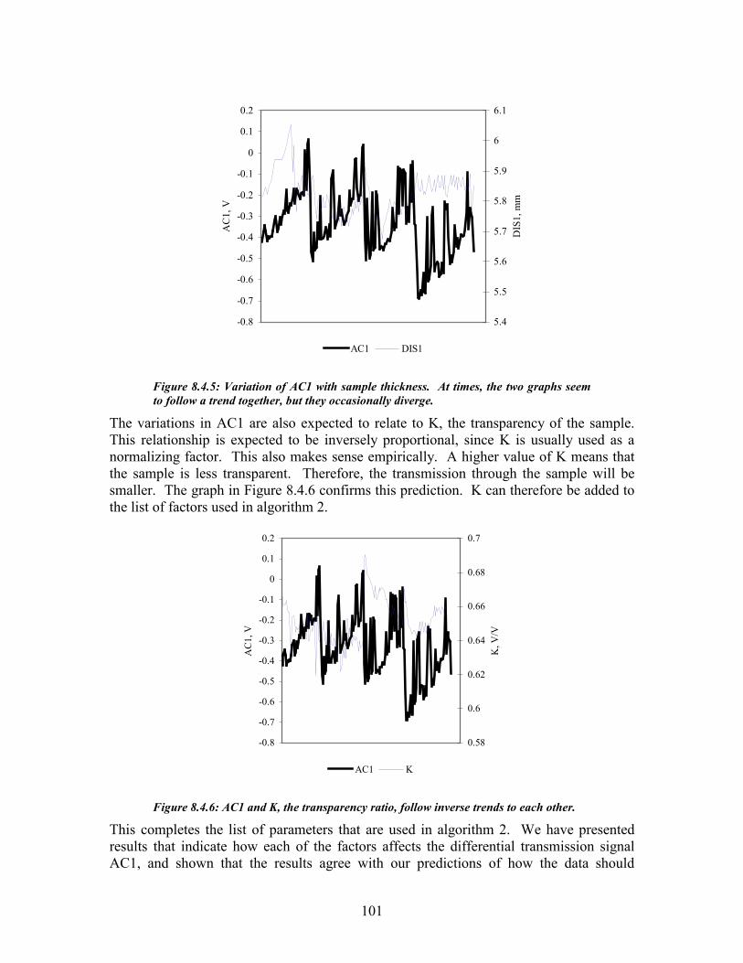
101
-0.8
-0.7
-0.6
-0.5
-0.4
-0.3
-0.2
-0.1
0
0.1
0.2
AC
1, V
5.4
5.5
5.6
5.7
5.8
5.9
6
6.1
DIS
1, m
m
AC1 DIS1
Figure 8.4.5: Variation of AC1 with sample thickness. At times, the two graphs seem to follow a trend together, but they occasionally diverge.
The variations in AC1 are also expected to relate to K, the transparency of the sample. This relationship is expected to be inversely proportional, since K is usually used as a normalizing factor. This also makes sense empirically. A higher value of K means that the sample is less transparent. Therefore, the transmission through the sample will be smaller. The graph in Figure 8.4.6 confirms this prediction. K can therefore be added to the list of factors used in algorithm 2.
-0.8
-0.7
-0.6
-0.5
-0.4
-0.3
-0.2
-0.1
0
0.1
0.2
AC
1, V
0.58
0.6
0.62
0.64
0.66
0.68
0.7
K, V
/V
AC1 K
Figure 8.4.6: AC1 and K, the transparency ratio, follow inverse trends to each other.
This completes the list of parameters that are used in algorithm 2. We have presented results that indicate how each of the factors affects the differential transmission signal AC1, and shown that the results agree with our predictions of how the data should

102
behave. In the following section, we present results of the MLR fitting of these parameters to develop algorithm 2.
8.4.2 Model Development Results The results described in the previous section were used to arrive at a list of twelve parameters that will be fit by a least-squares algorithm to the data to obtain a urea concentration estimate. Forty measurements were performed on each of three different samples. This data was then used as a training set, with the actual urea content of the sample being used as the desired output. The least-square fitting is a computation intensive technique, but it can be easily handled for this many variables by MS-Excel. The results of the least-square fit are given in Table 8.4.1. The results of the fit are given in several parts. First, we wish to know how strongly the urea estimate obtained from the algorithm relates to the actual value for this training data set. This is given by the R2 value, which is 0.982. Second, we need a measure of how significant the regression equation is. The information can be determined from the ANOVA table that is given in the second part of Table 8.4.1. The important values are F and the significance of F. Note that the value of F, 444.8 satisfies the rule of F=10R described in the previous chapter. The significance value is the probability that a similar data set could have occurred by chance. The value of 2.4⋅10-87 means that this probability is very low. The final part of Table 8.4.1 gives the relative weights for each parameter used in the algorithm, along with a standard error for the weight, a student’s T statistic, and a p-value for the parameter. Not all of the variables in the algorithm are significant (to a level of 0.05) according to the p-value. The inclusion of insignificant variables in the model is not wrong, but they may not have a strong effect on the quality of the model [80]. We have chosen to leave them in because they provide a modest improvement in the accuracy of the model, and because we have reason to include them based on our knowledge of the system.

103
Table 8.4.1: MLS Result Table: urea in water study.
Regression Statistics R Square 0.980 Observations 121 ANOVA
df SS MS F Significance FRegression 13 440306.7 33869.8 444.8 2.4E-87 Residual 108 8908.2 82.5 Total 121 449214.96
Variable Name Coefficients Standard Error
(mg/dl) t Stat P-value Intercept -193676.3587 15117.9 -12.8 2.1E-23 REF_WL 135.9786546 10.8 12.5 8.5E-23 OFFSET 2462.927493 212.8 11.6 1.3E-20 SAMPLET0 -297.1233721 18.1 -16.4 4.6E-31 SAMPLET1 419.3035103 19.6 21.3 1.5E-40 DIS1 -107.9165421 18.6 -5.8 6.7E-08 K 827.21904 18.6 44.5 2.9E-71 AC0 -63.45139936 106.3 -0.6 5.5E-01 AC1 -1353.567637 1251.3 -1.1 2.8E-01 ACC1 3456.430981 3772.5 0.9 3.6E-01 DELK00 17651.44236 8053. 1 2.2 3.1E-02 DELK0 -8667.813973 3803. 9 -2.3 2.5E-02 DELK1 -5371.793321 4707.1 -1.1 2.6E-01 The standard error of calibration for this model is 8.7mg/dl.
8.4.3 Results of urea estimation model application Now that algorithm 2 has been developed, we need to test it to see if it is able to predict urea values from new samples. A new test was run approximately 1 week later with a new sample. The algorithm accurately predicted the urea concentration of the sample. The standard error of prediction was found to be 9.2 mg/dl. The standard error for all of the tests that were run using this instrument are summarized in Table 8.4.2.
Table 8.4.2: Results of Urea Estimation Study
Model Std Error
8.7 mg/dl (1.4 mM) Prediction Std Error
9.2 mg/dl (1.5 mM) The number of samples tested for this study is admittedly small, since the true test of the system is in measuring hemodialysis samples, as described in the following section. The real purpose of this part of the study was to obtain data with which to generate the algorithm, rather than to test the prediction capabilities of this algorithm. We shall now describe the results of the hemodialysis patient studies and the application of algorithm 2

104
to the resulting data. The resulting calibration curve (estimated urea vs. true urea) is shown in Figure 8.4.7.
Estimated vs. Actual Urea
0
50
100
150
200
250
0 50 100 150 200 250
Actual Urea, mg/dl
Estim
ated
Ure
a, m
g/dl
Figure 8.4.7: Calibration curve for urea in water studies: estimated urea vs. actual urea (R2 = 0.97). Actual urea content was determined by weight (accurate to 0.1 mg) when samples were prepared.
8.5 Results of the Urea Level Estimation Studies: Hemodialysis Patient Studies This section is intended to explain the results of the hemodialysis sample studies that were performed using the second generation NIV prototype. First, the results of the measurement using algorithm 1 will be presented. As was stated in the introduction to this chapter, this algorithm could not be used to successfully estimate the urea level of the samples. The remainder of this section will then show how algorithm 2 (described in the previous section and in Chapter 7) was applied to this data. We will show how successfully this algorithm is able to estimate the sample urea concentration when applied to the data, even in the presence of multiple other analytes. Finally, we will show that the results indicate that the algorithm is able to fulfill the performance goals laid out in Chapter 2.
8.5.1 Results of Application of Algorithm 1 As with the urea in water studies, it is not possible to use algorithm 1 to estimate the urea concentration of a dialysate sample using this method. The results of this study when algorithm 1 is applied to the data are shown in Figure 8.5.1. The calibration line shows no sensitivity to urea.

105
0
2
4
6
8
10
0 10 20 30 40
Measured Urea, mg/dlPr
edic
ted
Ure
a, m
g/dl
Figure 8.5.1: Urea Estimation Calibration curve for algorithm 1. Urea content of the samples was measured using a Beckman CX7 autoanalyzer. The algorithm shows no predictive power for this study (R2 = 0.002).
8.5.2 Model Development Results Because this study was performed on an instrument with different hardware characteristics than the urea in water studies, it was necessary to recalibrate the algorithm. The parameter list developed in this chapter and in Chapter 7 does not change, since the basic operating characteristics of the instrument have not changed. However, as some gains in the hardware have changed significantly, the weight of each parameter in the algorithm should be adjusted. In order to recalibrate the algorithm we selected three patient samples at random from all of the samples obtained at the dialysis center. These three samples were each measured twenty times, and the data recorded. These 60 data sets were then used to train the least-squares algorithm in the same manner as the urea in water study. The actual value of the urea level of the sample was assessed by a standard Biuret method using a Beckman CX7 autoanalyzer. We were able to produce a significant model from this data as well. A summary of the regression statistics for this model is given in Table 8.5.1. The R2 value was 0.986, and the F value is far greater than 10R. We can conclude that this model has a high degree of statistical significance. In the parameter list, all variables are highly statistically significant except for AC00, ACC1 and DELK1. This is to be expected, since they were highly corrupted with noise and other variations to start with. Including them in the model is not wrong, it is simply unlikely that they cause significant improvement in the accuracy of the model [80]. They are allowed to remain in the algorithm because there is physical and mathematical basis for including them (see §7.4). The standard error of the model was 0.4 mg/dl. This represents a significant (over 20 times) improvement from the urea in water studies. This can be attributed to an improved sample handling technique, and higher signal to noise

106
ratio in the prototype version of the instrument used for this study than the previous study. Note that removing the non-significant parameters from the algorithm changes the standard error to 0.9 mg/dl. This result is still within the limits of acceptable clinical accuracy, but does justify the inclusion of the extra factors. Conversely, if even one of the significant parameters (such as SAMPLET0) is removed, the model loses a great deal of accuracy. By removing SAMPLET0, for example, the standard error of prediction rose to 10.7 mg/dl.
Table 8.5.1: MLS Result Table: Hemodialysis sample study.
Regression Statistics R Square 0.986 Observations 154 ANOVA
Df SS MS F Significance F Regression 13 644.3 49. 6 278.8 7.6-40 Residual 47 9.1 0.2 Total 60 653.3
Variable Name Coefficients Standard Error t Stat P-value Intercept -3793.048861 186.68 -20.3 6.4E-25 REF_WL 2.738386369 0.14 19.6 2.9-24 OFFSET 11.78231559 0.82 14.3 9.4E-19 SAMPLET0 -15.08450145 2.73 -5.5 1.4E-06 SAMPLET1 8.278386882 2.90 2.9 0.0064 DIS1 21.1473092 1.89 11.2 7.0E-15 K 17.11947157 1.89 9.1 6.6E-12 AC00 8.097130604 6.03 1.3 0.19 AC0 20.2117165 5.95 3.4 0.0014 ACC1 266.3492255 253.97 1.0 0.30 DELK00 -40175.72805 15445.25 -2.6 0.012 DELK0 39278.75765 15406.57 2.5 0.014 DELK1 -5.857607611 458.60 -0.01 0.99 The resulting calibration curve is shown below in Figure 8.5.2.

107
Urea Estimation Algorithm Model Fit
0
2
4
6
8
10
12
14
0 5 10 15Measured urea (mg/dl)
mod
el u
rea
(mg/
dl)
Figure 8.5.2: Calibration curve of measured urea vs. estimated urea. Measured urea content of the samples was determined using a Beckman CX7 autoanalyzer. Data resulted from repeated analysis of three randomly selected patient samples (R2 = 0.99, N=60).
8.5.3 Results of urea estimation model application Once the system was recalibrated using the training data set, it was necessary to test whether or not the algorithm could fulfill its goal of remaining valid for any patient sample over a period of at least one week. In order to make sure that the study was statistically significant, we needed to ensure that we measured an appropriate number of samples. The required sample size for a given study is given by the following formula:
2�
��
� ⋅=d
zn σ , (8.1)
where z is computed from the normal distribution for a desired p value, σ is an estimate of the standard deviation, and d is the number of units that we are willing to accept on either side of σ. Urea values in dialysate have been previously shown to be normally distributed. From the urea in water studies, we expected σ to be approximately 9 mg/dl. (The true value is lower, but we are really looking for a ratio of σ to d, so the number is still valid.) We want d to be no more than this on either side, so d = 4.5 mg/dl. We wish to establish significance at the 0.01 level, so z = 2.58. (The value of z is obtained from a normal distribution table). Substituting these numbers into the formula gives n=26.6. Therefore, at least 27 samples are required. We actually measured 34 samples, three of which were used in the calibration. Each sample was measured three times to allow for repeated measurements if necessary. The independently measured urea concentration was not known at the time the algorithm was applied to prevent bias in the results. It was important to establish whether or not the algorithm would remain valid without recalibration over time. Therefore, the samples were analyzed in two batches

108
approximately one week apart. No degradation of performance was seen over that time. In addition, the algorithm was able to successfully predict the urea concentration of all samples. No sample was rejected or yielded a result that was outside of acceptable accuracy limits. The standard error of prediction for the algorithm over all of the remaining samples was 0.5 mg/dl. The overall standard error including both calibration and prediction was 0.4 mg/dl. These figures are summarized in Table 8.5.2.
Table 8.5.2: Results of the MLS urea estimation algorithm: hemodialysis study
Model Std Error
0.4 mg/dl (0.07 mM) Prediction Std Error
0.5 mg/dl (0.08 mM) Overall Std Error
0.4 mg/dl (0.07 mM) Figure 8.5.3 shows the results of this study in the form of a scatter diagram. Estimated urea values produced by algorithm 2 are shown plotted against the measured urea values obtained from the standard instrument. The plot is highly linear and has a very strong correlation coefficient.
Estimated vs. Measured Dialysate Urea
0
5
10
15
20
25
30
35
40
0 10 20 30 40
measured urea (mg/dl)
pred
icte
d ur
ea (m
g/dl
)
Figure 8.5.3: Scatter diagram for the hemodialysis patient study. The plot shows that the algorithm could be used to accurately predict the urea concentration of the sample (R2 = 0.997, N=154).

109
Once these results were obtained, several other statistical pieces of information should be determined in order to further evaluate the performance of the instrument. First, we wish to determine if there is any mean difference between the values given by our instrument and the conventional instrument. This can be done with a simple hypothesis test. The null hypothesis is that the mean difference between the results given by the two instruments is less than 0.05 mg/dl. We choose α = 0.01. Therefore, using a student’s t test, the critical value of t for α =0.01 and 153 degrees of freedom is -2.4. The test statistic here is the mean of the errors (0.03) – the hypothesized difference (0.05) divided by the square root of the standard deviation (0.4) multiplied by n (154). The value of the test statistic is -0.4. Since this is in the acceptance region, we can conclude that the true mean difference between the two instruments is less than 0.05 mg/dl, with a p value of 0.001. Next, we can determine a 95% confidence interval for the variance ratio of the two instruments using an F-test. The result of this analysis is the conclusion that the true variance ratio between our method and the standard method is between 0.7 and 1.5 with 95% confidence. The final test of the data is the linear regression analysis between the standard method and algorithm 2. The summary of this analysis appears in Table 8.5.3.
Table 8.5.3: ANOVA table comparing the urea results obtained with the MLS algorithm to the clinical standard instrument.
Regression Statistics R Square 0.996 Standard Error 0.4 Observations 153 ANOVA
df SS MS F Significance FRegression 1 6658.5 6658.5 33575.4 2.9E-179 Residual 151 29.9 0.2 Total 152 6688.5
Coefficients Standard Error
(mg/dl) t Stat P-value Intercept -0.05495066 0.06 -0.9 0.37 Slope 1.010141649 0.006 183.2 2.9E-179 The results of this analysis allow us to conclude that this algorithm is able to fulfill its goals of providing a stable, universal means of estimating the urea content of a hemodialysis sample over the clinically expected range of urea values.
8.6 Results of Phantom Model Testing To prevent phantom modeling, we took precautions to ensure that our data did not contain any profiling information. Each sample was taken from a different patient, and the samples were taken at random times during the dialysis process. In addition, the

110
samples were analyzed in a random order. This precludes any time-dependent variable from affecting the results. In addition, we repeated the Arnold experiment [83] by applying our algorithm to: a) randomly assigned urea values; and, b) time dependent profiles (linearly increasing and decreasing). For the randomly assigned urea profiles, the R2 value for the model ranged from 0.04 to 0.38. The standard error of prediction (SEP) was usually about 30 mg/dl. For the linearly increasing profile, the R2 value for the model was 0.96. However, when the model was applied to the data, the calibration no longer held, and the R2 value was approximately 0.05. The SEP was 44 mg/dl. For the linearly decreasing profile, similar results were obtained, with an R2 value of 0.04 and an SEP of 44 mg/dl. For the model alone, the R2 value was 0.989, but the F-value was only 7.0, which does not satisfy the F=10R rule. Therefore, we can conclude that this model holds little predictive power when applied this type of linear profile. For the random case, ratio of F to R was usually about 0.04, showing that this model has extremely low significance. We can then conclude that if the model holds higher predictive power compared to the true urea values of the patient samples, the correlation is not due to some time-dependent phenomenon.
8.7 Medical Interpretation of Estimated Urea Level Results and Projected Use for Dialysis Efficiency Monitoring
The estimated urea content of the dialysate over time is a good parameter for estimating the efficiency of dialysis. This parameter can be used to estimate the urea removal rate, or to calculate the total urea removed over the course of a dialysis session. There is little widespread agreement as to what constitutes the optimum urea removal rate or how much total urea is removed, so the decision of what constitutes adequate therapy from these numbers is widely left to the discretion of the physician.

111
9 DISCUSSION In this chapter, a discussion of the urea monitoring system development is presented, as well as an analysis of the results achieved from testing of the instrument. The development process and the final version of the instrument and urea monitoring algorithm are described. Next, the testing protocol and results are discussed, including difficulties encountered during the testing process. Finally, the performance of the instrument and accompanying algorithm are discussed and analyzed.
9.1 Urea Monitoring System Instrument Design The Urea Monitoring Instrument developed during the course of this research was tested and evaluated with a series of in vitro studies. During this process, important conclusions concerning the performance of the instrument were made that provided direction for future improvements in the system. This information will lead towards development of future generations of the instrument. This first generation instrument did not possess sufficient capabilities to accurately measure urea levels in solution. It was capable of generating light at the appropriate wavelengths for measuring urea, but the instrument had several insurmountable problems. First, the quality of the optical components used in the design was not high enough to provide adequate light intensity to the sample. (High quality optical components could not be obtained due to the limited budget of the project). For this reason, a high gain was required, leading to a poor signal to noise ratio. The SNR for this system was on the order of 15 dB. In addition, the covered channel design of the system conducted too much heat in an uncontrolled manner to the sample, resulting in a high degree of drift in the measurement. Drift values as high as 100 mg/dl per hour were often observed when testing this system. The high degree of drift made it difficult to establish whether or not the system was responding to the presence of urea. The instrument fulfilled the design goals in terms of light generation, control, and measurement, but the effect of uncontrolled temperature variations on the instrument were stronger than expected, preventing the system from achieving the desired accuracy. Once the problems with this instrument were identified, it became apparent that the necessary modifications were not feasible. Further testing therefore continued with an existing prototype that possessed higher quality optical components and better temperature stability. The existing prototype (referred to as the NIV instrument), originally developed for a separate research project was designed to measure glucose levels in earlobe tissue. Modifications were made to this instrument to permit in-vitro testing of urea by the development of a special fluid cuvette. Preliminary tests with this instrument also showed significant drift, although the noise level was significantly lower. The SNR for this system is closer to 60 dB. The drift seemed to be caused by temperature changes in the sample and in differences in sample thickness caused by variations in the way the cuvette was assembled for each measurement. Despite these

112
improvements, the standard error of the measurements was still extremely high, and baseline shifts prevented any calibration from holding true for more than one sample. It became apparent that temperature variations had a large effect on the in-vitro measurements and they prevented accurate determination of urea levels.
9.2 Urea Monitoring Algorithm Design At this point, the focus of our experiments shifted towards developing a new algorithm that would be able to correct for these and other variations in the data. This new algorithm provided the means to extract information about the urea content of the sample from data obtained from the NIV prototype instrument. Using this algorithm, a significant improvement in performance was achieved with this instrument over both the old algorithm and the first generation prototype. Level shifting and baseline drift were completely eliminated, and measurements and calibrations remained stable for several months. The standard error of the measurements was reduced from well above 30 mg/dl to less than 0.5 mg/dl. The algorithm completely met the stated goal of being able to estimate the urea level of a hemodialysis sample from the instrument data. This algorithm represents significant advances over previous versions. For the first time, a stable, universal calibration was achieved. Previous versions of the algorithm required a strict set of operating conditions for the instrument that often were not met. This resulted in a large number of rejected measurements. The older versions of the algorithm did not remain valid as the sample was changed. The new algorithm is able to function over the full set of operating conditions for the instrument, and remains accurate for sample changes. In addition, this algorithm also compensates for temperature variations in the sample that cause large changes in the signals obtained from the instrument. In short, the algorithm developed during the course of this research makes possible the accurate reagentless monitoring of dialysate urea level where previous algorithms have failed.
9.3 Proof of Principle Studies These experiments were performed using the NIV prototype in conjunction with a specially designed in vitro cuvette. This presented some challenges and difficulties in the experimental procedure. In this section, these difficulties are explained, and in some cases solutions for overcoming them are presented. Any features of the measurements that yielded interesting results are also discussed.
9.3.1 Baseline Studies Protocol The baseline studies provided a large amount of useful data in determining how variations in the system affected the measurement. This data was then analyzed to arrive at the urea monitoring algorithm. Some difficulties were encountered when performing these measurements however. The NIV instrument was originally designed to measure on a human ear lobe. Designing a cuvette that could hold two separate fluid and displace one presented a serious design challenge in terms of space and shape considerations. The resulting cuvette was adequate for the job, but was not very user-friendly. A stepwise

113
assembly procedure had to be completed each time the sample was changed, and the quality of the results were somewhat dependent on the assembly technique. If the screws holding the cuvette together were not adequately tightened, fluid could leak out of the cuvette. Also, if the membrane surfaces separating the two fluids were not in contact with the sample, air bubbles occurred that degraded the quality of the results. Finally, due to the irregular geometry of the measurement head, it was impossible to place the cuvette in the same location each time. Improper placement of the cuvette could lead to poor compression of the sample, which also worsens the measurement accuracy. The algorithm is generally able to detect and compensate for these problems, but they do still contribute to errors. Most notably the transparency ratio approaches 1 when an air bubble or improper placement occurs. The instrument then warns the user to replace the sample. After a bit of practice, we gained significant experience in proper assembly and placement of the cuvette. This experience helped to improve the accuracy of the measurement over the course of this research. Future work with this method should include a redesign of the measurement head and cuvette to automate sample filling, along with a snap fit design to ensure exact placement.
9.3.2 Baseline Studies Testing Results These studies yielded several important results that aided in the development of the urea estimation algorithm. First, the responses of several system variables to fluctuations in temperature were quantified. Temperature was found to have a very large effect on the magnitude of the optical transmission signals recorded from the instrument. Almost all of the baseline drift that occurred in the measurements could be attributed to temperature variations in the sample. Thickness of the sample was also determined to have an effect on the measurement. The baseline studies also allowed us to extract a set of parameters that could be used to model variations in the instrument that are unrelated to the presence of urea in the sample, and to eliminate factors that were redundant from the analysis. Factors such as the reference wavelength and offset required to balance the system prior to measurement are also related to the temperature variations due to the dependence of optical spectra on temperature. The baseline studies also showed how the transmission signal varies with sample transparency. Finally, a set of parameters that identified how the residual AC signals after balancing affected the outcome of the measurement. The identification of parameters explaining variation in the instrument data provided by the baseline study was a crucial step in the development of the urea estimation algorithm. Previously, the information contained in the data related to urea content of the sample was mixed with that of the instrumental variation. This study provided a successful means of deconvolving the urea information from the instrumental variations. In addition, the added knowledge of how the instrumental variations affected the data allowed for a wider range of operating parameters for the measurement. This reduces some of the performance demands on the instrument, and also significantly reduces the number of rejected measurements. Using the old algorithm, 10-20% of all measurements
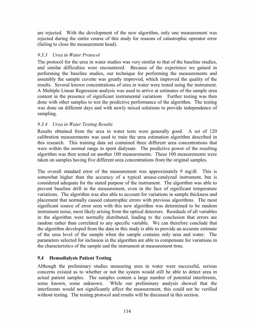
114
are rejected. With the development of the new algorithm, only one measurement was rejected during the entire course of this study for reasons of catastrophic operator error (failing to close the measurement head).
9.3.3 Urea in Water Protocol The protocol for the urea in water studies was very similar to that of the baseline studies, and similar difficulties were encountered. Because of the experience we gained in performing the baseline studies, our technique for performing the measurements and assembly the sample cuvette was greatly improved, which improved the quality of the results. Several known concentrations of urea in water were tested using the instrument. A Multiple Linear Regression analysis was used to arrive at estimates of the sample urea content in the presence of significant instrumental variations Further testing was then done with other samples to test the predictive performance of the algorithm. The testing was done on different days and with newly mixed solutions to provide independence of sampling.
9.3.4 Urea in Water Testing Results Results obtained from the urea in water tests were generally good. A set of 120 calibration measurements was used to train the urea estimation algorithm described in this research. This training data set contained three different urea concentrations that were within the normal range in spent dialysate. The predictive power of the resulting algorithm was then tested on another 100 measurements. These 100 measurements were taken on samples having five different urea concentrations from the original samples. The overall standard error of the measurement was approximately 9 mg/dl. This is somewhat higher than the accuracy of a typical urease-catalyzed instrument, but is considered adequate for the stated purpose of the instrument. The algorithm was able to prevent baseline drift in the measurement, even in the face of significant temperature variations. The algorithm was also able to account for variations in sample thickness and placement that normally caused catastrophic errors with previous algorithms. The most significant source of error seen with this new algorithm was determined to be random instrument noise, most likely arising from the optical detectors. Residuals of all variables in the algorithm were normally distributed, leading to the conclusion that errors are random rather than correlated to any specific variable. We can therefore conclude that the algorithm developed from the data in this study is able to provide an accurate estimate of the urea level of the sample when the sample contains only urea and water. The parameters selected for inclusion in the algorithm are able to compensate for variations in the characteristics of the sample and the instrument at measurement time.
9.4 Hemodialysis Patient Testing Although the preliminary studies measuring urea in water were successful, serious concerns existed as to whether or not the system would still be able to detect urea in actual patient samples. The samples contain a large number of potential interferents, some known, some unknown. While our preliminary analysis showed that the interferents would not significantly affect the measurement, this could not be verified without testing. The testing protocol and results will be discussed in this section.

115
9.4.1 Hemodialysis Patient Testing Protocol We did not encounter any significant new problems when testing the hemodialysis patient samples. A third generation NIV prototype was used for these studies, since it had a greater SNR than the previous instrument. Experience from the preliminary studies had helped to develop consistent sample handling techniques. Collection of the samples was relatively simple as well. Sessions at the dialysis center are organized into four daily shifts. Patients generally alternate days. Samples were taken from the drain line of the dialysis machine and put into a 50 ml container, then sealed. The samples were then marked with an identifying number and frozen until analysis. Sample collection did not disturb the patients. Although dialysis fluid is not considered a biohazard, a typical biohazard protocol was followed in terms of sample handling and workstation cleanup.
9.4.2 Hemodialysis Patient Testing Results Using the algorithm developed from the urea in water studies, we were able to accurately estimate the urea level of the patient dialysate samples. Three samples were measured repeatedly (20 times) to obtain a calibration for dialysis fluid. 31 additional samples were then analyzed, and the results were compared to results obtained using a reference method. Overall, the standard error of prediction was 0.34 mg/dl. This is well within acceptable clinical limits. The correlation coefficient between this algorithm and the reference method was 0.998, to a significance level of p<10-197. We were able to show that there was no mean difference between values given by our method compared with the reference method, and we found that the 95% confidence interval for the variance ratio of the two devices was very close to 1. We were able to conclude that the presence of other analytes in the dialysis fluid does not cause significant error in the measurement. The improved accuracy of this test over the urea in water tests can be attributed to two factors. First, our technique in performing the testing was improved by experience gained with earlier testing. Second, improvements in the NIV prototype had further lowered the noise level and improved the signal power. As with the urea testing, the residuals of the variables used in the algorithm were normally distributed, meaning that the measurement inaccuracy can be assumed to be random and therefore not significantly correlated with any of the other parameters. The measurement takes about 35 seconds to complete, and in this un-automated version takes about 3 minutes to set up. This is still well within the performance limits required for the measurement, which was specified to be 15 minutes. It is therefore possible to perform repeated measurements that would further improve the accuracy of this method. Most importantly, the algorithm remained valid for all patient samples that were tested over a period of over one week. Universal, stable calibration was hypothesized to be one of the main advantages of this algorithm over previous versions. The results of this study proved this hypothesis to be true.
9.5 Significance of Results The MLR approach has shown a significant increase in performance over the simple linear algorithm for the in vitro tests. Initial results using the linear algorithm were very

116
poor, having a standard deviation over 30 mg/dl and significant level shifts (sometimes over 100 mg/dl) when samples were changed. (Because of the level shifting, it is difficult to obtain a measure of the standard error.) When the MLR approach was used, the standard error was reduced to approximately 0.5 mg/dl, and the level shifts were eliminated. Temperature effects were shown to be the major cause of variations in the signal. The ANOVA showed incredibly high significance (p < 10-197 for urea, n=154). For the first time, a global calibration is possible that works for any patient tested over a wide range of operating conditions. This represents some significant advances:
• = Reduces the need for lengthy calibration procedures and permits the monitoring of acute patients
• = Dramatically reduces the number of rejected measurements by widening the acceptable operating limits of the instrument
• = Relaxes some of the performance requirements of the system hardware by providing compensation for deterministic effects and variations, thereby reducing the expense of the system.
To summarize, algorithm 2 as presented here provides the key to reagentless dialysate urea monitoring in a way that was not possible with previous versions of the algorithm. It provides long-term stability of results and universal calibration, and accomplishes its goal of being able to estimate sample urea concentration in the face of uncontrolled instrumental variations in the data.
9.6 Dialysis Monitoring System Testing Results While no dialysis efficiency monitoring was actually undertaken during this phase of the research, testing results have shown the feasibility of using this technique for dialysis monitoring. The system is capable of estimating dialysate urea levels in real-time and semi-continuously. The measurement frequency is sufficient to provide an accurate picture of the instantaneous urea level, the total urea removed, and the projected kT/V. Results have proven to be stable over the required monitoring period of one week, proving that the method can be used for the purpose of monitoring dialysis efficiency. In order to apply this method in the clinical setting, modifications to the existing instrument must be made to provide for automated operation.

117
10 CONCLUSION The overall goal of this research was to develop a method for optically monitoring the urea concentration of effluent dialysate without the need for reagents. No successful results have been reported on this topic to date. We were able to accomplish the research goal. By comparing the material presented in Chapters 4-9 of this dissertation with the specific aims of this research listed in Chapter 2, the following conclusions can be made: • = An Optical Bridge based instrument was developed and evaluated according to the
requirements stated in Chapter 2. The instrument was accompanied with special system software that controls the instrument and analyzes, stores, and displays the recorded data. This system software was developed for the MS-Windows 95/98 platform and was written in C/C++. The instrument fully satisfied the specifications set out in Specific Aim 1.
• = Preliminary studies were performed with this instrument using samples of distilled water spiked with urea. Existing algorithms failed to produce satisfactory results with this instrument. Large uncontrolled variations in sample temperature were determined to cause unacceptable drift and noise levels in the results. It was concluded at this point that the aluminum channel construction of the first prototype device prevented adequate temperature stability. All further testing was done with a second prototype that had better temperature control properties. Results using this instrument were somewhat improved, but still unsatisfactory.
• = We defined a list of factors that were hypothesized to cause instrumental variations. These factors may relate to non-random system noise or sample variations.
• = An algorithm relating data from the second instrument to the sample urea content was developed. When this algorithm is applied to the data, the noise and systematic error is significantly reduced. The algorithm can accurately predict urea concentration in dialysate, providing a measure of the efficiency of the dialysis session. While the data analysis has elucidated many previously unknown properties of the instrument, many properties still remain unexplored. We believe that significant effort should be expended to further explore these properties, and to extract parameters that can be used in the algorithm to represent them.
• = Preliminary in vitro patient studies were performed using the newly developed algorithm to determine the urea content of hemodialysis samples. The results of the study showed that this algorithm is capable of accurately determining the urea content of the dialysate sample, and therefore of providing useful data concerning the efficiency of the dialysis session. This specific aim was fully accomplished.
• = Using the results of these studies, we developed an algorithm for real-time estimation of dialysate urea level and real-time monitoring of dialysis efficiency. These algorithms were incorporated into the system software, and satisfy the requirements for this type of system. The development of this system represents a major advance in the field of renal failure therapy by providing the groundwork for a “closed loop”

118
approach to determining adequacy of therapy and eliminating the guesswork involved in current methods. The automatic, low maintenance nature of this system provides a high potential for clinical acceptance of the technology and the possibility of saving lives by reducing complications from poor dialysis.
In Chapter 3, Hypotheses and Research , four hypotheses were introduced that describe the central ideas of this work. We used the following scientific methods in the course of our research and hypothesis testing: statistical analysis of data, mathematical modeling, experimentation, induction, and deduction. The validity of these three hypotheses can now be evaluated based on the application of these scientific methods.
• = The first central hypothesis was that a method based on differences in transmission of near infrared light energy can be employed in the development of an instrument that could provide information about biologically relevant levels of urea in a strongly absorbing background matrix.
This hypothesis was accepted. An algorithm was developed that provides real-time estimates of dialysate urea levels from data recorded from such an instrument. Its evaluation showed that urea levels could be accurately determined for each and every patient sample that was tested, but only a limited number of disturbance variables was investigated. At this time, we can conclude that this method can provide an accurate means of estimating dialysate urea levels within the normal range of operation of the instrument.
• = The second central hypothesis was that it is possible to develop an algorithm using the data obtained from the instrument to quantitatively and qualitatively estimate the amount of urea in an effluent stream of dialysate, and from this to evaluate the effectiveness of the dialysis session.
This hypothesis is accepted. We developed and tested such an algorithm that is based on multiple linear regression analysis and time-wise integration of sample urea, and showed that it can be used to successfully monitor dialysate urea levels. From this information we would be able to provide a measure of dialysis efficiency. The accuracy of the measurement (<0.5 mg/dl) is approximately the same as traditional chemistry methods, and is considered acceptable for the stated purpose.
• = The third hypothesis is that a list of major factors affecting the system response can be developed.
There are a large number of factors affecting the system response that can be extracted from the instrument data. We have identified a set of factors that are capable of representing the system response sufficiently to establish a relationship between the data and the sample urea level. Therefore, this hypothesis is also accepted, with the caveat that further

119
research could provide more information regarding the optimal set of factors.
• = The fourth hypothesis is that a mathematical model and corresponding algorithm can be developed which approximate the expected response of the system to changing urea concentration in the presence of interferences such as temperature changes and the presence of other metabolic analytes.
Preliminary patient studies confirmed that the algorithm developed for this research could be used to determine the urea content of hemodialysis samples. Independent testing of the sample urea content showed high correlation with the results obtained using this algorithm even in the face of wide fluctuations in temperature, the presence of other analytes, and other varying instrument parameters. The absolute error between the estimated and measured sample urea level is in an acceptable range. Therefore, this hypothesis is also accepted.

120
11 FUTURE WORK The research presented here concludes the first prototype phase in the development of a clinical instrument for monitoring dialysis efficiency by real-time estimation of dialysate urea levels. At this point, the research should continue in the following areas: • = Development of a clinical instrument for dialysis efficiency monitoring, including a
redesign of the instrument head and sample cuvette to provide automated operation. • = Additional investigation for improvement of the proposed urea estimation method. • = Direct comparison of this dialysate-side method with existing blood side techniques
in clinical studies. The first two proposed research directions can be performed simultaneously. Development of a new clinical instrument and improvements in the method can be based on experience gained from the research described here. The design of an automated system would greatly reduced operator-induced variation in the measurement, and greatly reduce the amount of work required by the system operator. Once this newly developed system is complete, the true potential of this system can be put to the test by comparison with traditional blood side and other dialysate side methods of monitoring dialysis efficiency. Due to its ability to provide time-based information about urea removal rates, this system has the potential to provide new information on how urea is removed from the body by dialysis, representing a significant advance in knowledge of urea kinetics.
121
12 DISCLAIMER This thesis employed the hardware principle known as the optical bridge, which was invented by Hannu Harjunmaa, and is currently being developed by VivaScan Corporation. VivaScan Corporation was founded by Robert Peura for the purpose of commercializing a non-invasive blood glucose monitor. The main contribution of this dissertation is the development of an MLR based algorithm that provided the key element for the reagentless optical measurement of urea.

122
13 REFERENCES
[1] National Kidney Foundation Website. http://www.nkf.org . 2000.
[2] Alloatti, S., Molino, A., Manes, M., Bonfant, G., and Bosticardo, G. M., "On-line dialysate urea monitor: comparison with urea kinetics," Int J Artif Organs, vol. 18 pp. 548-552, 1995.
[3] Bosticardo, G. M., Avalle, U., Giacchino, F., Molino, A., and Alloatti, S., "Accuracy of an On-line Urea Monitor Compared with Urea Kinetic Model and Direct Dialysis Quantification," ASAIO Journal, vol. 40 pp. M426-M430, 1994.
[4] Calzavara, P., Calconi, G., Da Rin, G. C. E., and Paolini, F., "A new biosensor for continuous monitoring of the spent dialysate urea level in standard hemodialysis," Int J Artif Organs, vol. 21 pp. 147-150, 1998.
[5] Depner, T. A., Keshaviah, P. R., Ebben, J. P., Emerson, P. F., Collins, A. J., Jindal, K. K., Nissenson, A. R., Lazarus, J. M., and Pu, K., "Multicenter clinical validation of an on-line monitor of dialysis adequacy," J Am Soc Nephrol, vol. 7, no. 3, pp. 464-471, Mar. 1996.
[6] Garred, L. J., St.Amour, N. R., McReady, W. G., and Canaud, B. C., "Urea Kinetic Modeling with a Prototype Urea Sensor in the Spent Dialysate Stream," ASAIO Journal, vol. 39 pp. M337-M341, 1993.
[7] Jacobs, P., Suls, J., Sansen, W., and Hombrouckx, R., "A disposable urea sensor for continuous monitoring of hemodialysis efficiency," ASAIO J, vol. 39, no. 3, pp. M353-M358, July 1993.
[8] Keshaviah, P. R., Ebben, J. P., and Emerson, P. F., "On-line monitoring of the delivery of the hemodialysis prescription," Pediatr.Nephrol, vol. 9 Suppl pp. S2-S8, 1995.
[9] Marshall, M. R., Santamaria, P., and Collins, J. F., "Biostat 1000 and Daugirdas blood-based hemodialysis quantification: agreement and reproducibility," Am J Kidney Dis, vol. 31, no. 6, pp. 1011-1018, June 1998.
[10] Polaschegg, H. D., "Automatic, noninvasive intradialytic clearance measurement," Int J Artif Organs, vol. 16, no. 4, pp. 185-191, Apr. 1993.
[11] Smirthwaite, P. T., Fisher, A. C., Henderson, I. A., McGhee, J., Mokhtar, N., Simpson, K. H., Whitehead, A. J., and Gaylor, J. D., "Development of a blood urea monitoring system for the closed loop control of dialysis," ASAIO J, vol. 39, no. 3, pp. M342-M347, July 1993.
123
[12] Morbidity and Mortality of Dialysis: NIH Consensus Statement Online 1993. http://services.medscape.com/govmt/NIH/1999/guidelines/NIH-dialysis/nih1102.01.html . 1993.
[13] Delmez, J. A. and Windus, D. W., "Hemodialysis Prescription and Delivery in a Metropolitan Community," Kidney Int, vol. 41 pp. 1023-1028, 1992.
[14] Gotch, F. A. and Sargent, J. A., "A Mechanistic Analysis of the National Cooperative Dialysis Study," Kidney Int, vol. 28 pp. 526-538, 1985.
[15] Lindsay, R. M., Heidenheim, A. P., Spanner, E., Baird, J., Simpson, K., and Allison, M. E., "Urea Monitoring During Dialysis: The Wave of the Future," ASAIO Transactions, vol. 37 pp. 49-53, 1991.
[16] Lowrie, E. G. and Lew, N. L., "Death Risk in Hemodialysis Patients," Am J Kidney Dis, vol. 15 pp. 458-482, 1990.
[17] Babb, A. L., Popovich, R. P., Christopher, T. G., and Scribner, B. H., "The genesis of the square meter-hour hypothesis," Trans Am Soc Artif Intern Organs, vol. 17 pp. 81-91, 1971.
[18] Cheng, Y. L., Shek, C. C., Wong, F. K., Choi, K. S., Chau, K. F., Ing, T. S., and Li, C. S., "Determination of the Solute Removal Index for Urea by Using a Partial Spent Dialysate Collection Method," Am J Kidney Dis, vol. 31, no. 6, pp. 986-990, 1998.
[19] Cheung, A. K., "Quantitation of Dialysis: The importance of Membrane and Middle Molecules," Blood Purif, vol. 12 pp. 42-53, 1994.
[20] Chiari, L., Cappello, A., Tartarini, R., Paolini, F., and Calzavara, P., "Model-based dialysis adequacy prediction by continuous dialysate urea monitoring," Int J Artif Organs, vol. 21 pp. 526-534, 1998.
[21] Collins, A. J. and Keshaviah, P., "Are there limitations to shortening dialysis treatment?," ASAIO Transactions, vol. 34, no. 1, pp. 1-5, 1988.
[22] Collins, A. J., Ma, J. Z., Umen, A., and Keshaviah, P., "Urea index and other predictors of hemodialysis patient survival," Am J Kidney Dis, vol. 23, no. 2, pp. 272-282, 1994.
[23] Collins, A. J., Ma, J. Z., Umen, A., and Keshaviah, P., "Urea index and other predictors of hemodialysis patient survival [published erratum appears in Am J Kidney Dis 1994 Jul;24(1):157]," Am J Kidney Dis, vol. 23, no. 2, pp. 272-282, Feb. 1994.
[24] Daugirdas, J. T., Depner, T. A., Gotch, F. A., Greene, T., Keshaviah, P., Levin, N. W., and Schulman, G., "Comparison of methods to predict equilibrated kT/V in the HEMO Pilot Study," Kidney Int, vol. 52, no. 5, pp. 1395-1405, Nov. 1997.

124
[25] Depner, T. A., Greene, T., Gotch, F. A., Daugirdas, J. T., Keshaviah, P. R., and Star, R. A., "Imprecision of the hemodialysis does when measured directly from urea removal," Kidney Int, vol. 55 pp. 635-647, 1999.
[26] Garred, L. J., Rittau, M., McCready, W., and Canaud, B., "Urea kinetic modelling by partial dialysate collection," Int J Artif Organs, vol. 12 pp. 96-102, 1989.
[27] Garred, L. J., DiGiuseppe, B., Chand, W., McCready, W., and Canaud, B., "kT/V and Protein Catabolic Rate Determination from Serial Urea Measurement in the Dialysate Effluent Stream," Artificial Organs, vol. 16, no. 3, pp. 248-255, 1992.
[28] Gotch, F. A., Sargent, J. A., and Peters, J. H., "Studies on the molecular etiology of uremia," Kidney Int Supp, vol. 7 pp. S276-S279, 1975.
[29] Hall, J. W. and Pollard, A., "Near-infrared spectroscopic determination of serum total proteins, albumin, globulins, and urea," Clin Biochem., vol. 26, no. 6, pp. 483-490, Dec. 1993.
[30] Hornberger, J. C., "The hemodialysis prescription and quality-adjusted life expectancy. Renal Physicians Association Working Committee on Clinical Guidelines," J Am Soc Nephrol, vol. 4, no. 4, pp. 1004-1020, Oct. 1993.
[31] Ijelu, G. and Raja, R. M., "kT/V and Hemodialysis Morbidity Revisted," ASAIO Transactions, vol. 36 pp. M152-M154, 1990.
[32] Ilstrup, K., Hanson, G., Shapiro, W., and Keshaviah, P., "Examining the foundations of urea kinetics," Trans Am Soc Artif Intern Organs, vol. 31 pp. 164-168, 1985.
[33] Jacobs, P., Sansen, W., and Hombrouckx, R., "Continuous Monitoring of the Spent Dialysate Urea Level Using a Disposable Biosensor," ASAIO Journal, vol. 40 pp. M393-M400, 1994.
[34] Keshaviah, P., "A technological assessment of the current and future status of hemodialysis," Med Instrum, vol. 20, no. 2, pp. 65-73, 1986.
[35] Keshaviah, P., "The solute removal index--a unified basis for comparing disparate therapies [editorial]," Perit.Dial Int, vol. 15, no. 2, pp. 101-104, 1995.
[36] Kessler, E., Ritchey, N. P. C. F., Caccamo, L. P., Carter, K. J., and Erickson, B. A., "Urea Reduction Ratio and Urea Kinetic Modeling: A Mathematical Analysis of Changing Dialysis Parameters," Am J Nephrol, vol. 18 pp. 471-477, 1998.
[37] Kopple, J. D., Jones, M. R., Keshaviah, P. R., Berstrom, J., Lindsay, R. M., Moran, J., Nolph, K. D., and Teehan, B. P., "A Proposed Glossary of Dialysis Kinetics," Am J Kidney Dis, vol. 26, no. 6, pp. 963-981, 1995.

125
[38] Maasrani, M., Jaffrin, M. Y., Fischbach, M., and Boudailliez, B., "Urea, Creatinine, and Phosphate Kinetic Modeling During Dialysis: application to pediatric hemodialysis," Int J Artif Organs, vol. 18 pp. 122-129, 1995.
[39] Mendley, S. R., Majkowski, N. L., and Higgins, P. K., "Estimation of Urea and Creatinine Clearance in Peritoneal Dialysis," ASAIO Journal, vol. 38 pp. M373-M376, 1992.
[40] Nolph, K. D., Keshaviah, P., Emerson, P., Van Stone, J. C., Twardowski, Z. J., Khanna, R., Moore, H. L., Collins, A., and Edward, A., "A new approach to optimizing urea clearances in hemodialysis and continuous ambulatory peritoneal dialysis," ASAIO J, vol. 41, no. 3, pp. M446-M451, July 1995.
[41] Orellana, A., Martinez-Fabregas, E., and Alegret, S., "On-line monitoring of urea in effluent liquid during haemodialysis," J Pharm.Biomed.Anal., vol. 11, no. 10, pp. 921-926, Oct. 1993.
[42] Petitclerc, T., Bene, B., Jacobs, C., Jaudon, M. C., and Goux, N., "Non-invasive monitoring of effective dialysis dose delivered to the haemodialysis patient," Nephrol Dial Transplant, vol. 10, no. 2, pp. 212-216, 1995.
[43] Petitclerc, T., "Estimation of mass transfer through a hemodialyzer: theoretical approach and clinical applications," Artif Organs, vol. 22, no. 7, pp. 601-607, July 1998.
[44] Raj, D. S., Tobe, S., Saiphoo, C., and Manuel, M. A., "Quantitative dialysis using two dialysate samples: a simple, practical and accurate approach for evaluating urea kinetics," Int J Artif Organs, vol. 20 pp. 422-427, 1997.
[45] Ronco, C., Brendolan, A., Crepaldi, C., Frisone, P., Ghiotto, F., Zamboni, S., Gastaldon, F., and La Greca, G., "On-line urea monitoring: a further step towards adequate dialysis prescription and delivery," Int J Artif Organs, vol. 18, no. 9, pp. 534-543, Sept. 1995.
[46] Vanholder, R. C. and Ringoir, S., "Adequacy of Dialysis: A Critical Approach," Kidney Int, vol. 42 pp. 540-558, 1992.
[47] Vanholder, R. C., "Assessment of Urea and Other Uremic Markers for Quantification of Dialysis Efficiency," Clin Chem, vol. 38, no. 8, pp. 1429-1436, 1992.
[48] Vanholder, R. C., Hsu, C., and Ringoir, S., "Biochemical Definition of the Uremic Syndrome and Possible Therapeutic Implications," Artificial Organs, vol. 17, no. 4, pp. 234-239, 1993.
[49] Hemodialysis: Principles and Practice Academic Press Inc., 1972.

126
[50] Black, R. M. Head of Renal Medicine, St.Vincent's Hospital: Personal Communication, 2000.
[51] Kupcinskas R, Harjunmaa H, Kun S, and Peura R. “Urea Clearance Monitoring During Dialysis Using an Optical Bridge Method: Feasibility Studies”. 24th Annual Northeast Bioengineering Conference, Hershey, PA. 1998.
[52] Harjunmaa, H. Method for Determining by Absorptions of Radiations the Concentration of Substances in Absorbing and Turbid Matrices. [US Patent #5099123]. 1992.
[53] Harjunmaa, H., Peura, R. A., and Mendelson, Y. Method and Apparatus for Measuring the Concentration of Absorbing Substances. [US Patent #5112124]. 1992.
[54] Harjunmaa, H., Mendelson, Y., and Wang, Y. Electromagnetic Method and Apparatus to Measure Constituents of Human or Animal Tissue. [US Patent #5183042]. 1993.
[55] Harjunmaa, H., Mendelson, Y., and Wang, Y. Electromagnetic Method and Apparatus to Measure Constituents of Human or Animal Tissue. [US Patent #5178142]. 1993.
[56] Harjunmaa, H. Chief Scientist, VivaScan Corporation: Personal Communication, 2000.
[57] Fox, S. I., Human Physiology, 4th ed. Wm. C. Brown Publishers, 1993.
[58] "Dialysis fluid composition and quality - professional opinion vs scientific evidence: Report on the Dialysis Opinion Lunch Symposium at the ERA-EDTA Congress, 23 September 1997, Geneva," Nephrol Dial Transplant, vol. 13 pp. 1598-1602, 1998.
[59] Bailey, J. L. and Mitch, W. E., "Metabolic Acidosis as a Uremic Toxin," Sem Nephrol, vol. 16, no. 3, pp. 160-166, 1996.
[60] Bailey, J. L. and Mitch, W. E., "The search for the uremic toxin: the case for metabolic acidosis," Wien Klin Wochenschr, vol. 109, no. 1, pp. 7-12, 1997.
[61] Bakir, A., Williams, R. H., Shaykh, M., Dunea, G., and Dubin, A., "Biochemistry of the uremic syndrome," Adv.Clin Chem, vol. 29 pp. 61-120, 1992.
[62] Brunner, H. and Brunner, A., "[Dialyzability of possible "uremia toxins"]," Med Welt, vol. 27, no. 47, pp. 2264-2266, Nov. 1976.
[63] De Smet, R., Glorieux, G., Hsu, C., and Vanholder, R., "p-cresol and uric acid: two old uremic toxins revisited," Kidney Int Suppl, vol. 62 pp. S8-11, Nov. 1997.
127
[64] Gordon, A., Berstrom, J., Furst, P., and Zimmerman, L., "Separation and characterization of uremic metabolites in biologic fluids: a screening approach to the definition of uremic toxins," Kidney Int Suppl, no. 2, pp. 45-51, Jan. 1975.
[65] Hsu, C. H. and Patel, S. R., "Uremic toxins and vitamin D metabolism," Kidney Int Suppl, vol. 62 pp. S65-S68, Nov. 1997.
[66] Kraus, L. M. and Kraus, A. P., Jr., "The search for the uremic toxin: the case for carbamoylation of amino acids and proteins," Wien Klin Wochenschr, vol. 110, no. 15, pp. 521-530, 1998.
[67] Niwa, T., "Mass Spectrometry in the Search for Uremic Toxins," Mass Spectrom Rev, vol. 16, no. 6, pp. 307-332, 1997.
[68] Ringoir, S., "An Update on Uremic Toxins," Kidney Int Suppl, vol. 52, no. Suppl. 62, pp. S-2, 1997.
[69] Schoots, A. C., Mikkers, F. E., Claessens, H. A., De Smet, R., Van Landschoot, N., and Ringoir, S. M., "Characterization of uremic "middle molecular" fractions by gas chromatography, mass spectrometry, isotachophoresis, and liquid chromatography," Clin Chem, vol. 28, no. 1, pp. 45-49, Jan. 1982.
[70] Schreiner, G., "The search for the uremix toxin(s)," Kidney Int Supp, vol. 7 pp. S270-S2791, 1975.
[71] Medical Reference Library, 3rd ed. NY: John Wiley & Sons, 1989.
[72] Zubay, G., Biochemistry, 3rd ed. Wm. C. Brown Publishers, 1993.
[73] Sternby, J., "Whole Body Kt/V from Dialysate Urea Measurements during Hemodialysis," J Am Soc Nephrol, vol. 9 pp. 2118-2123, 1998.
[74] Aldrich FT-IR Library of Spectra of Organic Compounds NY: Aldrich Publishing Co, 1989.
[75] Bellamy, L. J., The Infrared Spectrum of Complex Molecules: Advances in Infrared Group Frequencies Chapman and Hall, 1980.
[76] Silverstein, R. M., Clayton Bassler, G., and Morrill, T. C., Spectrophotometric Identification of Organic Compounds, 5th ed. John Wiley & Sons, 1991.
[77] Daniel, W. W., Biostatistics: A Foundation for the Health Sciences New York: John Wiley & Sons, 1991.
[78] Murdock, J. R., "Development of Measurement Modules for a Reagentless Chemistry Analyzer." Masters Thesis, Worcester Polytechnic Institute Library, 2000.

128
[79] Geigy Scientific Tables West Caldwell, NJ: Medical Education Division, Ciba-Geigy Corporation, 1984.
[80] Kish, L., Statistical Design for Research New York: John Wiley & Sons, Inc., 1987.
[81] Lindsey, J. K., Models for Repeated Measurements New York: Oxford University Press, 1993.
[82] Draper, N. R. and Smith, H., Applied Regression Analysis, 3rd ed. New York: Wiley & Sons, 1998.
[83] Arnold, M. A., Burmeister, J. J., and Small, G. W., "Phantom glucose calibration models from simulated noninvasive human near-infrared spectra," Anal.Chem, vol. 70, no. 9, pp. 1773-1781, May1998.
[84] Puri, M. L. and Sen, P. K., Nonparametric Methods in General Linear Models New York: John Wiley & Sons, Inc., 1985.
[85] Sheskin, D. J., Handbook of Parametric and Nonparametric Statistical Procedures New York: CRC Press, 1997.