Embed Size (px)
Citation preview
JOURNAL OF MOLECULAR SPECTROSCOPY 67, 132-156 (1977)
A Method for Merging the Results of Separate Least-Squares
Fits and Testing for Systematic Errors
D. L. ALBRITTON AND A. L. SCHMELTEKOPF
Aeronomy Laboratory, NOAA Environmental Research Laboratories, Boulder, Colorado 80302
AND
R. N. ZARE
Department of Chemistry, Columbia University, New York, New York 10027
A method is presented for merging the results of separate least-squares fits to obtain the
most precise, single values for each of the molecular constants of a spectroscopic system. The
output molecular constants and accompanying variance-covariance matrices from each of
the separate fits are taken together as input to a correlated least-squares fit, which then yields
the desired merged single values. The method is applied to a X-r8 diatomic model band
system using well-defined synthetic data as an example. Other currently used, multistate
methods of obtaining molecular constants for a spectroscopic system are special cases of the
method described here. For the nonlinear least-squares fits required for multiplet states, the
merge method is particularly advantageous. The properties of the merged values of the
molecular constants and their standard errors are examined with regard to forming confidence
limits for these estimates and it is shown that, in most spectroscopic applications, the con-
fidence limits have their usual meaning. Furthermore, it is similarly shown that the confidence
limits for the variance of the merged fit provide a simple and convenient test for the presence
of relative systematic errors between the separate least-squares results being merged. Although
the method is illustrated here by merged separate band-by-band results, it also can be applied
to any type of spectroscopic results.
INTRODUCTION
The band plays a central role in the analysis of molecular spectra. For example, the
recognition of the band structure of a spectrum and the branch patterns of each band
are the first steps in the assignment of vibrational and rotational quantum numbers.
Furthermore, once the assignments are complete, the measured line positions of a band
system are commonly grouped and tabulated by bands. Consequently, it is not sur-
prising that, among the several approaches of reducing a band system to molecular
constants,r one popular way has been to make a least-squares fit of the calculated line
1 Other approaches to reducing a system of bands to molecular constants involve two steps: first, the
construction of intermediate “data,” such as combination differences or term values, that pertain to
the vibrational levels of each electronic state separately, and second, the independent fitting of a rota-
tional Hamiltonian to the intermediate “data” of each vibrational level to obtain the molecular con-
stants of that level. These indirect, or one-state, approaches therefore differ distinctly from the direct, or multistate, approach employed in the band-by-band reduction discussed here. The former approach fits
132
Copyright 0 1977 by Academic Press, Inc.
All rights of reproduction in any form reserved. ISSN 0022-2852
MERGING SEPARATE LEAST-SQUARES RESULTS 133
positions derived from upper- and lower-state rotational Hamiltonians to the measured
line positions of each band separately. Such a band-by-band reduction of a system of
bands has the appeal of treating the data set conveniently in multiple “bite sizes,” in
contrast to a huge simultaneous multiband fit involving the Hamiltonians of all upper and lower vibrational levels and all of the measured line positions of all of the bands.
However, in almost all instances, many of the bands of a molecular band system will share common upper or lower vibrational levels. For such redundant systems, a band- by-band reduction will produce multiple values for each of the molecular constants of
the common vibrational levels. Clearly, to halt the analysis of the band system at this point is undesirable, since the presence of multiple values for a constant indicates a
missed opportunity, namely, the opportunity to treat the system as a whole and obtain a “best” single value for the molecular constant that, ideally, is more precise than that
obtained from any one band separately. When using the band-by-band reduction method, many approximate ways have been
used to treat the system as a whole. One way would be to simply average all of the multiple values for each constant. However, this would ignore, among other things, the generally different precision of each value. Even the more preferable weighted average
would ignore the often strong correlations (3, Section D-2-c) that generally exist between the errors of many pairs of molecular constants. Another approximate method of com- bining results of substantially different precision has been to simply hold certain con-
stants in a least-squares fit jixeti to separately obtained, high-precision values and then to determine values and errors for the remainder of the constants. Familiar examples of this are fixing to microwave results in fits to electronic bands, or fixing to combination-
difference results for the zeroth vibrational level in a set of absorption bands. Clearly, this procedure assumes that the errors associated with the fixed values are negligible
in comparison to the others. While this can be a good assumption in some cases, there are many cases where it is not. If the relative precision is not manyfold, then the assump- tion of no error in the fixed values usually means that the error estimates obtained for the
other constants are too small. Rather than these approximate approaches, which require special cases to be valid, what is needed is a general technique.
We present here a method of ‘(merging” the results of band-by-band fits to obtain the “best” single value for each of the molecular constants and show that this method (a) can yield the identical results as the huge simultaneous fit mentioned above, (b) is much more practical for nonlinear applications, and (c), as a bonus, provides a convenient quantitative indication of possible relative systematic errors between bands. Thus, the convenient “bite sizes” of the band-by-band fit and the enhanced precision available from treating a redundant band system as a whole are both achieved. Although the
with a~ Hamiltonian at a time; the Iatter approach fits with more than one Hamiltonian at a time.
Both approaches have their merits and demerits. For example, the direct, multistate approach has the
capability of using all of the measured lines in its reduction, whereas, the indirect, one-state approach
cannot, in general. On the other hand, the direct, two-state approach cannot be applied if one of the
rotational Hamiltonians in a band cannot be specified adequately (e.g., perturbations); whereas, the
indirect? one-state approach can still be applied to obtain the constants of the state whose Hamiltonian
can be specified. The details of these two different approaches have been examined recently by Alhritton
cl ol. (I), dslund (Z), and Pliva and Telfair (3). Although the present paper applies the merge method
to only the direct, or multistate, approach, it can be applied equally well in all of these approaches.

134 ALBRITTON, SCHMELTEKOPF AND ZARE
ability to test for relative systematic errors between bands arises somewhat as a dividend of this method, it may in time prove to be its most valuable feature, since such errors among the far-flung bands of an extensive band system are almost unavoidable.
We illustrate the merge method by applying it to a lZ-% diatomic band system. How- ever, the method is not limited to this simple example, but applies equally well to electronic, infrared, Raman, and/or microwave data for transitions between or within
molecular states of any multiplicity of diatomic and polyatomic molecules to determine the minimum-variance estimates of term values, combination differences, molecular
constants, and/or Dunham-type coefficients, giving proper statistical regard to different measurement precision and correlation.
MERGED BAND-BY-BAND FITS
The present method has been applied to the bands of the HClf A%+-X*Il system (5) and to the O,+ b4Zg-a411u system in an accompanying paper (6), but here we apply it to a simple, but nevertheless realistic, band system that is designed to most clearly
illustrate the features of the method.
Model Bad System
Figure 1 schematically shows the three bands of a model lZ-lZ system. Two electronic transitions are included : a (0,O) band having the first 50 R lines and the first 50 P lines
and a (0, 1) band having the first 2.5 R lines and the first 25 P lines. In addition, the
model system contains one infrared transition: the (1, 0) fundamental vibration-
rotation band having the first 50 R lines and the first 50 P lines. It is clear that the model system has considerable redundancy. A band-by-band reduction will produce two values for each of the rotational constants B, and D, of each vibrational level and
will yield values for three band origins, one of which is related to the other two. Finally, each of the bands has at least one vibrational level in common with at least one other band, which is a necessary condition for treating a system as a whole. For example, a
(1, 2) band could not be combined with these bands.
Bond 1 Burld 2
(O,O) (0.11 EleCfrOnlC Electronic 100 Lines 50 ll”ezS.
CT =0.05 cm- 0=0.05cme’
T” 8” 0” Band 3 11 ,I ,
Fundamental “lbrat,on-Ro,a,lo”
100 Lines
““20 u=0.005cm-’
E” 01 D” 0
Lower ‘H Elecfronic Slate
FIG. 1. _The structure of themodel band system. Tw” -10.
MERGING SEPARATE LEAST-SQUARES RESULTS
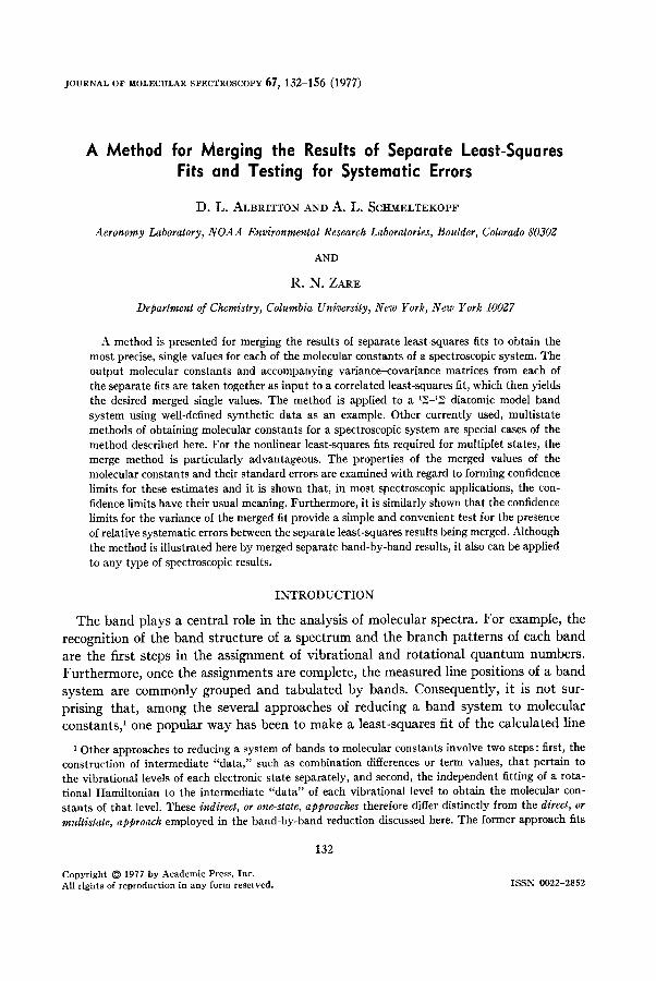
‘Table I. “True” Molrculnr Constants Used to Construct the Synthetic I.incs”
13.5
Bmd 1 hid 2
CO,01 CO,11
Rand 3
fundamental
“0 12000 1oonn ?.,,m
B 1.5 1.5 0
II;, 6.0 x 10 -6 6.” x 10-6
,I Bl 0 !I s 0.98
II 3 5.5 x 10 -6 5 . 5 x 1 0 -6
B” 0 1.0 1.0
II
"0 5.0 x 10 -6 5.0 x 10 -6
a 0.05 0.05 0.005
a All units are reciprocal centimeters.
Rather than use laboratory data for three bands of these types for some particular molecule from the literature, it is much more informative here to use “synthetic data,” which offer far more flexibility in probing individual features of the method. (For examples of previous similar uses of such synthetic data, see Refs. (3, 4, 7).) In par- ticular, a set of synthetic data for the three bands of Fig. 1 is created by (a) calculating ‘Lexact” line positions from the “true” molecular constants in Table I using the well- known energy level expressions for diatomic ‘2; states (8), and (b), to these “exact” line positions, adding random, normally distributed “errors” with specified standard
deviations to form the “measured” line positions. Representative values for standard deviations were used here: u = 0.05 cm-l for the two electronic bands and (r = 0.005 cm-’ for the infrared band. It is to be emphasized that the values used for the molecular
constants and standard deviations are completely arbitrary; the values used here are given only to be specific.
Bauttl-by-BaTstd Least-Squares Fits
A band-by-band reduction of the model system in Fig. 1 requires three separate least- squares fits. Corresponding to the commonly made assumptions (4, Section C-2) that the measurement errors of each band R (k = 1, 2, and 3) are randomly scattered with variance ug2 and zero covariance, then the fit to each band is the usual unweighted, uncorrelated least-squares solution (4, Section D) of the overdetermined matrix equation
Yk = &es + Q, k = 1, 2, and 3,
where yk, @k, and ek are the column vectors containing the nk known measured line positions, the five desired molecular constants YO, B’, D’, B”, and D”, and the @k un-
136 ALBRITTON, SCHMELTEKOPF AND ZARE
Table II. A Set of Estimated Molecular Constants From a Band-by-Band Reductiona
Band 1 Band 2 Band 3
(0,O) (O>l) fundamental
-
YO 12000.007(10) 10000.009(13) 2000.00027(92)
,.I 80 1.49959(22) 1.49934(56)
..1 DO 5.879(68)X 10-6 5.30(67) x 1" -6
^I, 81 0.97939(56) 0.979985(21)
^I?
n1 4.82(67) x 10 -6 5.49X2(62) x lo-'
^11 80 0.99961(22) 0.999986(21)
I?" 0
4.887(68) x 1O-6 4.9933(62) x 1O-6
d k
0.0529 0.0471 0.00482
Degrees of freedom 95 45 95
a The numbers in parentheses are the uncertainty in the last digits that corresponds
to one standard error, i.e. 5.879(68) x 10 -6
= (5.879 2 0.068) x 10-8.
All. units are reciprocal centimeters.
known measurement errors, respectively, and Xk is the known %k X 5 coefficient matrix (see Ref. (4, Section D-l), for an example), all for the Kth band. The resulting least- squares values @k of the molecular constants are2
@k = ( &TXk)-lX~Tyk, & = 1, 2, and 3 (2)
and the accompanying variance-covariance matrix is
6, = 8k2(XbTX&l, k = 1, 2, and 3, (3)
where the estimated variance is
l&2 = (y!$ - Xkbk)T(Yk - Xk@k)/(fik - 5), k = 1, 2, and 3. (4)
The band-by-band reduction yields three sets of estimated molecular constants &, k = 1, 2, and 3, with five values per set, and three accompanying 5 X 5 variance- covariance matrices i$k, k = 1, 2, and 3. A set of estimated molecular constants that arise from one particular set of random errors is listed in Table II. The different precision of the estimates from bands 1 and 2 caused by the different number of lines in each band is readily apparent, particularly for the molecular constant DO’. Moreover, the different precision of the estimates from bands 1 and 3 due to the different precision of the measurement errors is also readily apparent, particularly for the molecular constant DO”. While the multiple values are very similar, as expected, they are not identical, as also expected, due to the random “measurement” errors. Considering the three-band system
* The notation follows that given in Ref. (4), Section B.
MERGING SEPARATE LEAST-SQUARES RESULTS
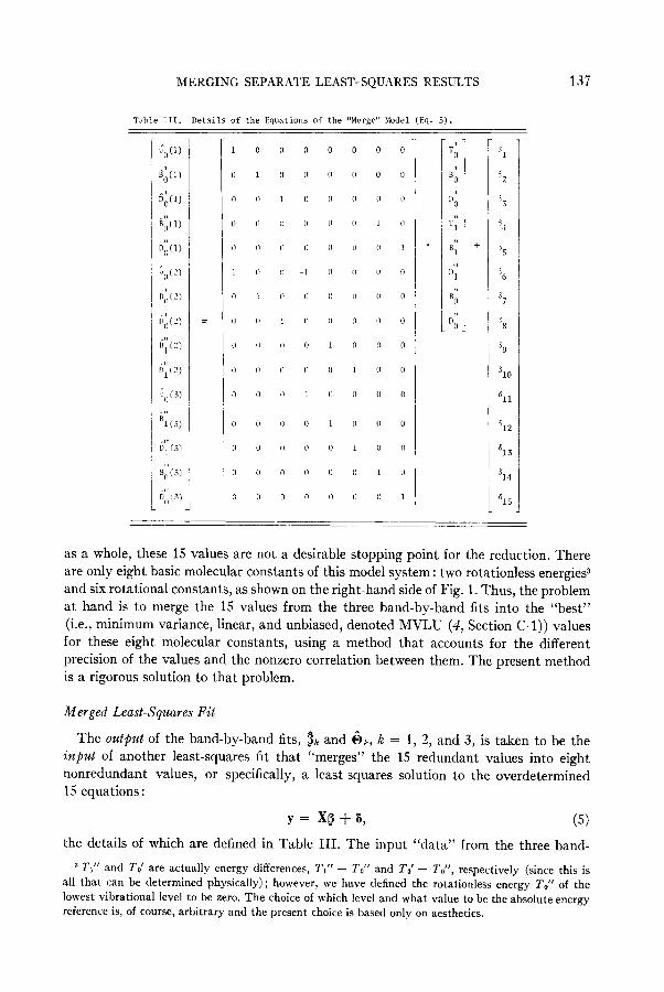
l’ahle III. Iktails of the Equations of the “Mer!ze” Hodcl (Ea. 5).
=
1
”
0
0
II
1
0
/1
0
I,
0
0
0
”
”
0
1
0
0
(1
0
1
0
”
”
0
0
0
0
0
”
0
1
/,
,I
0
II
1
(1
,l
0
0
0
(1
0
0
”
0
”
0
-1
(1
II
0
”
1
0
”
II
0
0
0
n
n
1
0
0
II
0
0
II
0
”
n
1
TO
B; "0
T;
” +
J
Bl ,I
Dl
7,
%
0
“0
137
as a whole, these 15 values are not a desirable stopping point for the reduction. There are only eight basic molecular constants of this model system : two rotationless energies3 and six rotational constants, as shown on the right-hand side of Fig. 1. Thus, the problem at hand is to merge the 15 values from the three band-by-band fits into the “best”
(i.e., minimum variance, linear, and unbiased, denoted MVLU (4, Section C-l)) values for these eight molecular constants, using a method that accounts for the different precision of the values and the nonzero correlation between them. The present method
is a rigorous solution to that problem.
Merged Least-Squares Fit
The output of the band-by-band fits, @k and 6k:, k = 1, 2, and 3, is taken to be the &put of another least-squares fit that “merges” the 15 redundant values into eight nonredundant values, or specifically, a least-squares solution to the overdetermined 15 equations :
y = X@ + 6, (5)
the details of which are defined in Table III. The input “data” from the three band-
3 T,” and TO’ are actually energy differences, TI” - TO” and TO’ - To”, respectively (since this is
all that can be determined physically); however, we have defined the rotationless energy To” of the
lowest vibrational level to be zero. The choice of which level and what value to be the absolute energy
reference is, of course, arbitrary and the present choice is based only on aesthetics.

138 ALBRITTON, SCHMELTEKOPF AND ZARE
by-band tits are stacked in the 15 elements of y, The eight nonredundant unknown constants are represented by 9. The coefficient matrix X relates the redundant values of y to the corresponding members of 0. For example, the second and seventh individual equations in the matrix Eq. (5) are
&‘(1) = Bo’ + 82, (5-2)
B,,‘(2) = B,,’ + 8,. (5-7)
They state that, except for the unknown errors & and 67, the values obtained for Bo’ in the fits to the first and second bands individually, 8,‘(l) and B,‘(2), respectively, should
be equal. Equation (5) also makes similar statements about the other redundant values. Of course, because of random measurement errors, the redundant values are almost
never equal. Therefore, the least-squares solution of Eq. (5) finds values for the molec- ular constants Q that minimize the sum of the squares of the unknown 6, subject to known
interrelations among the 6. In fact, recognizing that there are indeed interrelations among the unknown errors of the input values, &, k = 1, 2, and 3, is at the heart of the present
method. These interrelations arise because the variance-covariance matrices $k associated
with the @k, k = 1, 2, and 3, generally do not have equal diagonal elements and zero off-diagonal elements, i.e., 6k # 21, where c^ is a constant and I is the identity matrix.
To account for these unequal variances and nonzero covariances, the solution of Eq. (5) must employ the weighted, correlated least-squares formalism (4, Section F). Using this, the molecular constants that minimize 6’% subject to the interrelations contained
in $k, k = 1, 2, and 3, are given by
@” = (XT&-l X)-l XT&-ly, (6)
where & is the non&agonal 15 X 15 matrix composed of the individual 6k, A
01 0 0 i= 0 62 0 .
i 1
(7) 0 0 6)3
In addition to the circumflex A that denotes that the 0” values are MVLU estimates, we have added the superscript M to denote that they are estimates of the merged
method, a distinction that will be useful below. The precision of the estimates 8” is, of course, indicated by their standard errors,
which are the square roots of the diagonal elements of the variance-covariance matrix
associated with 8” : A $M = ,+&7M, (8)
where the merged dispersion matrix is given by
@ = (XT&X)--l. (9)
The estimated variance of the merged fit &,,I* is given by
8&r* = (y - X@M)G--l(y - X@M)/.&f, (10)
where the degrees of freedom of the merged fit are denoted by fin. For the example considered here, the degrees of freedom are f~ = 15 - 8 = 7.
MERGING SEPARATE LEAST-SQUARES RESULTS 130
Table IV. Merged Molecular Constants That
Correspond to the Band-by-Band
Results in Table IIa
1?000.0067(56)
l.J999501’5)
5,9815(9flj ‘: 111-6
‘olm.non:~~.~i
(1.9799R?(IhJ
5.49?1(49) I 10-h
0.99998?(16)
4.99?5(49) x 10.6
^ % li.RflJ
Degrees of freedom
7
a See the footnote of ‘Table II
Equations (l)-(10) define the merged band-by-band method. It is a two-step ap-
proach. The first step (Eqs. (l)-(4)) is a set of band-by-band fits4 to determine @k and
6k for each of the bands. The second step (Eqs. (5)-(10)) is a correlated fit to these output values to determine the “best” single values for the molecular constants of each
vibrational level. It is clear that the merged estimates oh’, 6”, and &r2 depend not only
on the redundant values ok, h = 1, 2, and 3, from the band-by-band fits, but also on
the accompanying variance-covariance matrices Gk, K = 1, 2, and 3, composing &.
The pervasive appearance of 4 in Eqs. (6)-(10) properly accounts for two features
of the input & making up y. First, the unequal diagonal elements of & account for the
fact that the input values y are generally of different precision. For example, the vari-
ances of the two values 8,‘(l) and B,‘(2) from the separate fits to bands 1 and 2,
respectively, differ by about a factor of six. The elements &z2 and $77 will account for
this by weighting the merged value for Bo’ toward 8,‘(l) by this factor.5 Secondly, the
4 The band-by-band fits are not limited to unweighted, uncorrelated least-squares formulations. If
the lines of a band are of different estimatable precision, then a weighted fit can be made. The correla-
tions among line position measurements are much more difficult to estimate reasonably and always have
been assumed to be zero.
6 This does not mean that the merged value for 230’ will be a factor-of-six weighted average of &o’(l)
and &d(Z), since there are many other interrelations involving Bo’ for which the merged fit wiil also
simultaneously account.
140 ALBRITTON, SCHMELTEKOPF AND ZARE
nonzero off-diagonal elements of & account for the fact that some of the input values are generally correlated (4, Section D-2-c). For example, the errors in 8,‘(l) of the upper state and 8,“(l) of the lower state are correlated with a coefficient of 0.9941. This means that the errors in 8,‘(l) and 8,“(l) are very likely to be of the same magnitude and sign. The nonzero off-diagonal element &a will account for this by weighting the difference of merged values of B,’ and Bo” toward the difference of 8,‘(l) and 8,“(l). Thus, 6 is a “generalized weight” matrix that simultaneously balances all of the diagonal and off-diagonal interrelations among the errors of y. Fundamentally, since
& is made up of the elements of bk2( Xkr X&r, K = 1, 2, and 3 (cf. Eqs. (3) and (7)),
it contains not only the information about the energy level expressions, but also the
differing rotational development and measurement precision among the bands, all of
which go into creating the interrelations.
Table IV gives the values that result from merging the band-by-band results in
Table II. Even though these are results that correspond to a particular set of random
“measurement” errors, Table IV does show some of the general features of merging the
band-by-band fits. Compared to Table II, there have been changes in both the precision
and the values of the molecular constants.
First, the precision (as indicated by the standard errors) of the molecular constants
of the 21’ = 0 level of the upper electronic state has improved considerably. For example,
the standard error associated with the merged value for Bo’ is a factor of 10 smaller than
that associated with the value for Bo’ obtained from the individual fit to band 1, the
most favorable of the two electronic bands (see Table II). This improvement is mainly
due to the fact that the high precision of the infrared band, which is associated only
with the lower electronic state, has been “propagated” into the upper electronic state
by the high correlation of the upper- and lower-state rotational constants of the two
electronic bands. It is interesting to note that this correlation has often been considered
a handicap in obtaining precise molecular constants ; here, it obviously is an advantage !
Such dramatic changes in the precision do not occur for the molecular constants of the
two levels of the lower electronic state because these levels are already dominated by
the more precise infrared band.
Secondly, the merged values for the molecular constants in Table IV differ, of course,
in varying degrees from the corresponding band-by-band results in Table II. Generally,
the merged results lie close to the more precise values from the band-by-band fit, namely,
those of the more rotationally developed electronic band and particularly the infrared
band. However, not all of the differences are what one might guess from such simple
considerations. Using the upper-state constant DO’ as an example, the merged value,
fi,,’ = 5.9815 X W6 cm-l, does lzot lie between the values obtained from the separate
fits to the two electronic bands, d<(l) = 5.879 X lO-‘j and &‘(2) = 5.30 X lO+ cm-‘.
Neither a simple average nor a weighted average based on the individual variances
could have predicted this, thereby indicating the role of the covariances, which place
strong interrelations on the values that highly correlated rotational constants can assume
simultaneously. Other properties of these merged estimates B”, GM, and dM2 will be
discussed below.
MERGING SEPARATE LEAST-SQUARES RESULTS 141
COMPARISON TO SIMULTANEOUS MULTIBAND LEAST-SQUARES FIT
The increase in precision gained by merging the results of the band-by-band fits is, of course, just the familiar statistical gain that occurs when a data set is enlarged.6 For
a molecular band system, this enlargement has, in the past, usually taken the form of combining all of the bands into a single, simultaneous multiband fit to obtain the best single values for the molecular constants of each vibrational level. For example, Plfva and Telfair (3) have explored the systematics of this gain for a simultaneous multiband
fit to an absorption band system with varying number of bands.
Weighted Simzdtaseous Multiband Least-Squares Fit
For the present example, a simultaneous multiband fit would be a single fit of the eight @ molecular constants (Fig. 1, right-hand side) to the 250 line positions yr, ys,
and y3 of the three bands. Since electronic and infrared bands are generally expected to have different measurement precision, this simultaneous fit should be a weighted least- squares fit (4, Section E). In the absence of more specific information, the simplest weighting scheme would be to assume that the electronic measurements are of equal precision and that the infrared measurements are also of equal precision, but are more
precise than the electronic. Thus, in the weighted fit, all of the electronic lines are assigned the same weight and all of the infrared lines could be assigned a greater weight, where the weights should be inversely proportional to some estimate of the generally
unknown measurement precision. For these estimates, one could simply assume that,
generally, infrared measurements are R times more precise than electronic measurements and could use weights of 1 and R2 for the electronic and infrared measurements, respec- tively.? However, this somewhat overly general assumption can be replaced by quanti- tative estimates of the electronic and infrared measurement precision. These could come from fits to each band separately, examples of which are given as the Bk values in Table II. Such a posteriori estimates are certainly generally preferable to a priori assumed ratios R. Thus, in the most general application, the weighted simzlltarseous
multiband method has, as its first step, a set of band-by-band fits. This is the same as
the first step of the merged band-by-band method, except that only the 8k2 are of interest here, not @k and 6,.
The second step is an estimation of the eight molecular constants 0 by a weighted least-squares solution (4, Section E) of the 250 equations
Yl = 219 + Yl,
with the weight of the lines yk of the Kth band being 1/6k2. The 250 X 8 matrix Z,
6 Because of this improvement in precision for the larger data set, it would appear wise to keep mar-
ginafly statistically significant molecular constants in the band-by-band Hamiltonians and delay the
final decision as to their significance until the increased precision of the enlarged data set permitted a
more sensitive test.
r In weighted least-squares fits, only the relative values of the weights influence the determination of
the molecular constants and their standard errors (3, Section E-Z).
142 ALBRIl”rON, SCHMELTEROPF AND ZARE
where Zr = [Zrr’Z~TZ~T], is unwieldy, but straightforward. (An example for a slightly different problem is given in Ref. (4), Eq. 19.) The weighted least-squares solution of Eq. (11) is
Here, the superscript W is used to specifically identify estimates obtained from the weighted simultaneous multiband fit. The variance-covariance matrix that accom-
panies 8” is given by $w = 6w2@v
> (13) where the dispersion matrix is
iTw = [ gr (ZkrZk/tG)]--1.
The estimated variance of the weighted fit is
C+wr = [ 5 (y!i - Z!JW)T(Yk - &@>/~21/fw,
(14)
(15)
where jw are the degrees of freedom. In the present example jw = 250 - 8 = 242.
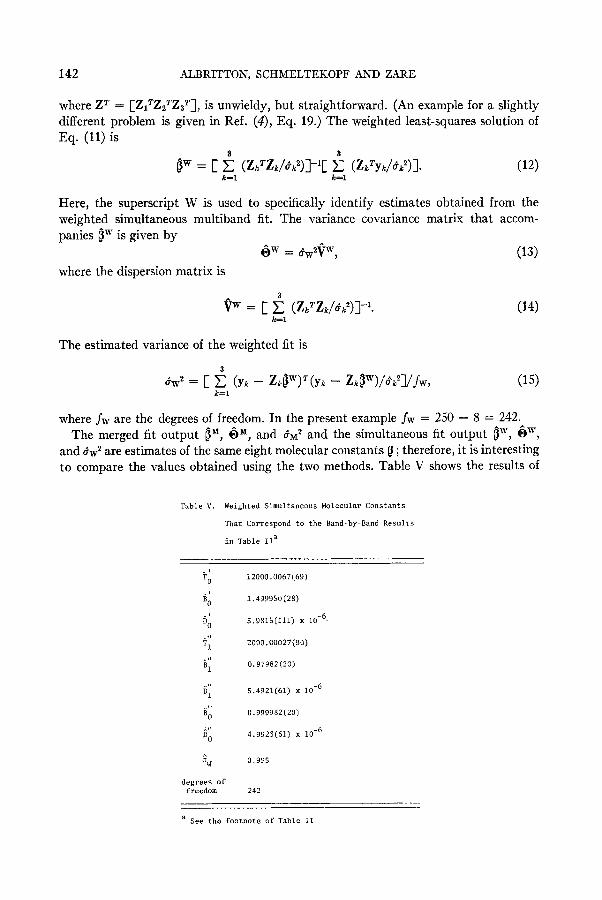
The merged fit output B”, @, and 8~~ and the simultaneous fit output Bw, QW, and Bw2 are estimates of the same eight molecular constants @ ; therefore, it is interesting to compare the values obtained using the two methods. Table V shows the results of
Table V. Weighted Simultaneous Molecular Constants
That Correspond to the Band-by-Band Results
in Table IIa
+l, 12000.0067(69)
"8
BO 1.499950(28)
^I DO
5.9815(111) x 10-6.
^!I =I 2000.00027(90)
-1) 81
0.97982(20)
"II D1 5.4921(61) x 10
-6
^(I BO 0.999982(20)
^I? DO
4.9923(61) x 1O-6
%I 0.995
degrees of freedom 242
a See the footnote of Table II
MERGING SEPARATE LEAST-SQUARES RESULTS 143
applying the weighted simultaneous multiband fit to the same example used in Tables II
and IV. The results are strikingly similar. In fact, starting with relations between the
X and 2 coefficient matrices, some tedious, but straightforward, matrix algebra shows
that
and
6” = @w, (16)
@l = +v 7 (17)
(C&i2 - l)/(Bw” - 1) = jw,/j&. (18)
These relations show that the weighted simultaneous multiband ft and merged barstl-by-
bad jit are equivalent. The results of one fit are either identical to, or can be derived from, the other. Since the first steps of these two methods are the same, the choice
between the two depends on the features of the second step. A comparison certainly appears to favor the merged fit. Once each of the bands have
been fitted to yield sets of ok and Gk, there is no need to handle the input line positions yk again, as would be required by the weighted simultaneous multiband fit; the merge
fit can get the same values for fj by handling only the compact sets of @k and hk. This is
much more convenient and should often require less computer storage. However, the most important factor is probably the fact that the second step of the merge method is always a linear fit. When the application involves the nonlinear Hamiltonians of higher-order multiplet electronic states, each band-by-band tit does, to be sure, involve a nonlinear tit to yield the molecular constants of the two vibrational levels. However, the second step of the merge method is always a linear least-squares fit, as given by
Eq. (6). This is in contrast to the second step of the simultaneous multiband method, in which a nonlinear fit must be made involving the molecular constants of all of the
vibrational levels. This generally expensive nonlinear second step clearly can be replaced by the less-expensive linear second step of the merged fit, since the results are equivalent. Discussion of other aspects of this comparison, particularly the consequences of Eq. (18),
will be deferred until a later section below.
l -nweighted Simultaneous Multibaml Least-Squares Fit
Many times, it has been implicitly assumed that all of the recorded bands involved have the same measurement precision. An example would be the bands of one electronic system that have been recorded in a relatively restricted wavelength region by the same investigator on one instrument over a relatively short time. In such applications, the simultaneous multiband fit is often shortened to one step, an unweighted least-squares tit to the lines of all bands to determine the values B”, QU, and 8u2, where U has been used to identify estimates obtained with this common unweighted variation of the simultaneous multiband fit. The equations yielding these estimates would be Eqs. (ll)- (15), with 6k8 = 1, k = 1, 2, and 3.
It is important to realize that the relations similar to Eqs. (16)-(B) do not rigorously apply now. Even though they seek estimates of @ from the same data, the two methods cannot be exactly equivalent because the least-squares models are different. As the price it must pay for its simplicity, the unweighted simultaneous multiband model involves the atZrlitio?zaZ assumption that all of the lines of all bands have the same
144 ALBRITTON, SCHMELTEKOPF AND ZARE
measurement precision. If this assumption is a good one, i.e., if all of the ch are nearly
equal, then
and
@W-@U (19)
QWE$J (20)
In addition to requiring this extra assumption, the unweighted simultaneous fit has a rather serious disadvantage of a practical nature. Since it is a one-step method, rela-
tively large least-squares fits must be made over and over during the inevitable cycles of discovering mispunched data cards, misassigned lines, inexplicably anomalous
measurements, and model testing (e.g., checking to see if H,’ and H,” are needed). This disadvantage is greatly magnified if the application is nonlinear, for reasons
similar to those mentioned above.
PROPERTIES OF THE MERGED ESTIMATES
Since the values 6 obtained from a least-squares fit are only estimates, it is necessary to indicate their quality. This is done by stating confidence limits (4, Section D-3-b), or more commonly, stating standard errors, from which the confidence limits can be
constructed. Such limits define the range about the estimated value pi in which the unknown pitrUe is believed, with a certain level of confidence, to lie. The establishment of confidence limits depends on the statistical properties of the estimates 8 and @,
which arise from, among other things, the statistical properties of the measurement errors. The latter are, of course, unknown; hence, recourse commonly is made to a set of ‘Lreasonable assumptions.”
In addition to assuming a correct physical model, the common least-squares assump- tions (4, Sections C-2 and D-3) are that the measurement errors are (i) normally distributed with (ii) zero mean and (iii) have a variance-covariance matrix u2@ that
is knows, except for the common factor u 2. Given these assumptions, well-defined confidence limits for the estimates @ from the familiar single-step least-squares method can be constructed straightforwardly by following prescribed procedures. The merged band-by-band method, however, is a two-step fit in which the output estimates from the first fit are used as input “data” to the second fit. As we shall see below, this feature can alter the statistical properties of the merged estimates o”, @, and a& in such a way that the confidence limits constructed from these estimates in the usual manner do not always have their normally expected, well-defined meaning. The origin of this loss of meaning of the merged confidence limits occurs between the first and second steps of the merged method. The output estimates from the first step must be examined with regard to the above three assumptions since they are the input to the correlated least-squares fit of the second step.
The assumption of normality causes no problem. If the measurement errors of the line positions yl, are normally distributed, as is commonly assumed,8 then it can be shown (9, p. 99) that the least-squares estimates from the first step @k are also normally
* The assumption of normally distributed measurement errors appears to be very realistic in most spectroscopic applications. There are simple tests with which its validity can be checked (see (4),
Section D-3-a for an example).
MERGING SEPARATE LEAST-SQUARES RESULTS 145
distributed. The assumption of zero mean requires that the systematic errors in both
the fitted model and the measurements of each band be much smaller than the random errors. While this assumption is almost always implicitly evoked, it is clear that it is
often violated. For the present purposes, it is also evoked here, but the consequences of its being violated are examined below.
The third assumption, that the variance-covariance matrix g,z& of the input y
(Eq. (5) and Table III) is Knoz~~ to within the common factor an,?, is the root of the
problem. The matrix & is only an estimate of the dispersion matrix, because it contains
the estimates kk2, k = 1, 2, and 3, of the measurement precision of the three bands. In
the following sections, the effects of this inadequate assumption on the confidence limits of (i) the merged estimates of the molecular constants 0” and (ii) the merged estimate
of the variance 6& are examined.
Confidence Limits for @”
In least-squares fits of f degrees of freedom where the above three assumptions are 4
met, it can be shown (9, p. 99) that the difference between the estimate pi and its un- known “true” value flitrue, divided by the standard error 6$, has a ‘9” distribution%
on f degrees of freedom, i.e., (ji - /P)/Bi$f - t(f). (21)
This means that if the set of measurements could be repeated many times in an identical
fashion, except for random measurement error, then the set of (pi - @P)/@i;~ values would be distributed symmetrically about zero in a fashion described by the t(f) func- tion, which is a commonly tabulated function of statistics. Stated alternatively and equivalently, the t(f) function describes the probability of occurrence of a given
(& - flitrue)/6i$ value. This property leads straightway (9, p. 107) to the familiar confidence interval (4, Section D-3-b)
[ji - t(f, 1 - G!/2)@)iit] < flitrUe 5 [JL + t(f, 1 - (Y/2)OiiB],
commonly abbreviated in the physical sciences as
(22a)
ji f t(“f, 1 - 42)&i:, (22b)
within which one can be lOO(1 - LY)~ 9 confident that the unknown “true” value fiitrUe
lies. Thus, in order to use Eq. (22b) to construct the same well-defined confidence limits for the merged estimates B”, it must be shown that the fraction (BiM - flLtrUe)/
(8iLM)+ is very nearly t distributed for the merged fit. In principle, the probability distribution of (biM - /3Pe)/(6iiM)” can be derived
algebraically using the approach that produced Eq. (21). However, the resulting algebra becomes exceedingly complicated, and since the end result is unlikely to be a commonly tabulated function, it would not have much utility. We have taken an alternate approach. The distribution of (piM - /3itrue)/(6iiM)i is generated by fitting 1000 sets of synthetic data described earlier. Each set differs from the others only because of the randomly generated, normally distributed “measurement” errors of mean zero and specified variance. Thus, the generated (@ - Pi”-)/(6ii”)” distribu-
*The t distribution is compared graphically to the similar and more familiar normal distribution
in Ref. (10, p. 81).
146 ALBRITTON, SCHMELTEKOPF AND ZARE
go)/
5
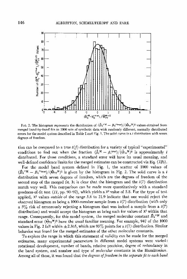
FIG. 2. The histogram represents the distribution of @o”~ - &I”~~~~)/(&~)* values obtained from
merged band-by-band fits to 1000 sets of synthetic data with randomly different, normally distributed
errors for the model system described in Table I and Fig. 1. The solid curve is a t distribution with seven
degrees of freedom.
tion can be compared to a true t(f) distribution for a variety of typical “experimental” conditions to find out when the fraction (biM - PLtrUe)/(BiiM)” is approximately t distributed. For those conditions, a standard error will have its usual meaning, and well-defined confidence limits for the merged estimates can be constructed via Eq. (22b).
For the model band system defined in Fig. 1, the scatter of 1000 values of (&“M - Bo “tr”“)/(&M)t ’ g’ 1s rven by the histogram in Fig. 2. The solid curve is a t
distribution with seven degrees of freedom, which are the degrees of freedom of the second step of the merged fit. It is clear that the histogram and the t(7) distribution match very well. This comparison can be made more quantitatively with a standard goodness-of-fit test (11, pp. 90-92), which yields a X2 value of 5.8. For the type of test applied, X2 values outside of the range 3.8 to 21.9 indicate that one would reject the observed histogram as being a lOOO-member sample from a t(7) distribution (with only a 5% risk of erroneously rejecting a histogram that was indeed a sample from a t(7) distribution) and would accept the histogram as being such for values of X2 within that range. Consequently, for this model system, the merged molecular constant Bo’lM and standard error (&r”)f have the usual familiar meaning. For example, 947 of the 1000 values in Fig. 2 fall within f2.365, which are 95% points for a t(7) distribution. Similar behavior was found for the merged estimates of the other molecular constants.
To explore the range in which this statement of validity can be made for the merged estimates, many experimental parameters in different model systems were varied: rotational development, number of bands, relative precision, degree of redundancy in the band system, and number and type of molecular constants in the Hamiltonian. Among all of these, it was found that the degrees of freedom in the separate_@ to each basd
MERGING SEPARATE LEAST-SQUARES RESULTS 147
/r ’
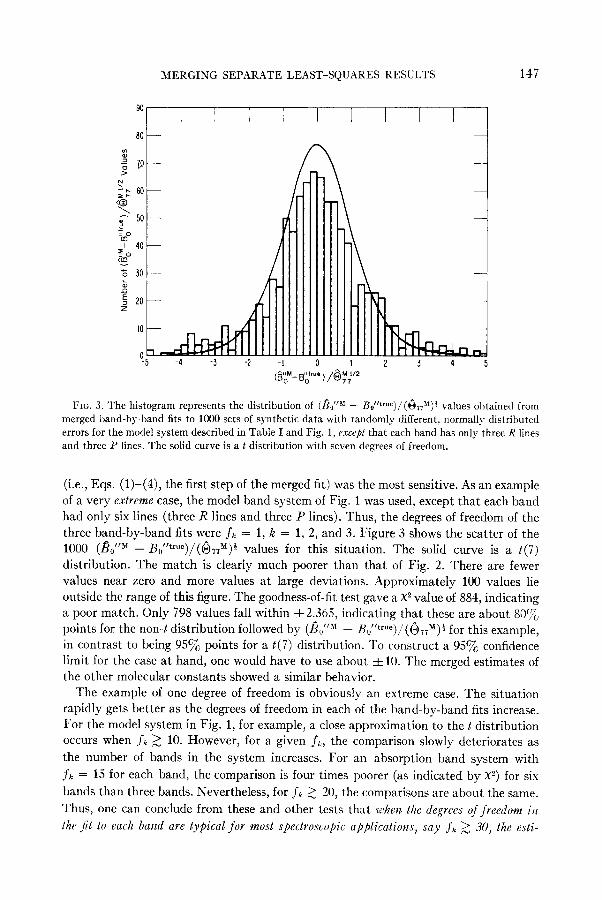
FIG. 3. The histogram represents the distribution of (8 ““>I - R0”truc)/(@)77 ) values obtained from .. 114
merged band-bp-band fits to 1000 sets of synthetic data with randomly different, normally distributed
errors for the model system described in Table I and Fig. 1, except that each band has only three R lines
and three P lines. The solid curve is a t distribution with seven degrees of freedom.
(i.e., Eqs. (l)-(4), the first step of the merged fit) was the most sensitive. As an example
of a very extreme case, the model band system of Fig. 1 was used, except that each band had only six lines (three R lines and three P lines). Thus, the degrees of freedom of the
three band-by-band fits were jk = 1, k = 1, 2, and 3. Figure 3 shows the scatter of the 1000 (&fJI - &“true )/(GTT”)” values for this situation. The solid curve is a t(7)
distribution. The match is clearly much poorer than that of Fig. 2. There are fewer
values near zero and more values at large deviations. Approximately 100 values lie outside the range of this figure. The goodness-of-fit test gave a X2 value of 884, indicating a poor match. Only 798 values fall within f2.365, indicating that these are about SOC~O points for the non-t distribution followed by (fi.,““’ - Hu”true )/(&J#)$ for this example, in contrast to being 95% points for a t(i) distribution. To construct a 95% confidence limit for the case at hand, one would have to use about f 10. The merged estimates of the other molecular constants showed a similar behavior.
The example of one degree of freedom is obviously an extreme case. The situation
rapidly gets better as the degrees of freedom in each of the band-by-band fits increase. For the model system in Fig. 1, for example, a close approximation to the t distribution occurs when jk 2 10. However, for a given jk, the comparison slowly deteriorates as
the number of bands in the system increases. For an absorption band system with
jk = 15 for each band, the comparison is four times poorer (as indicated by x2) for six
bands than three bands. Nevertheless, for jk 2 20, the comparisons are about the same.
Thus, one can conclude from these and other tests that ~kcrz the degrees oJ Jreedom in
t/w /it to ench band are typical for most spectroscopic czpplicatiofrs, say fk 2 30, the esti-
148 ALBRITTON, SCHMELTEKOPF AND ZARE
1. 4 5
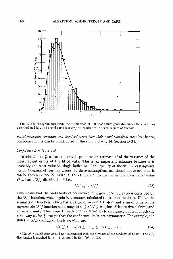
FIG. 4. The histogram represents the distribution of 1000 6 ~~ values generated under the conditions described in Fig. 2. The solid curve is a x2/j distribution with seven degrees of freedom.
mated molecular co&a&s and standard errors have their usual statistical meaning; hence, confidence limits can be constructed in the standard way (4, Section D-3-b).
Confidence Limits joy dM2
In addition to @, a least-squares fit produces an estimate a2 of the variance of the measurement errors of the fitted data. This is an important estimate because it is
probably the most valuable single indicator of the quality of the fit. In least-squares fits of f degrees of freedom where the three assumptions mentioned above are met, it can be shown (9, pp. 99-100) that the estimate b2 divided by its unknown “true” value u2tr,,e has a X2/f distribution,1° i.e.,
82/u2true - x2/f. (23)
This means that the probability of occurrence for a given 82/a2tr,e ratio is described by the X2/f function, which again is a common tabulated function of statistics. Unlike the symmetric t function, which has a range of - ~0 5 t 5 + 00 and a mean of zero, the asymmetric X2/f function has a range of 0 2 X2/f 5 a (since a2 is positive definite) and a mean of unity. This property leads (10, pp. 102-103) to confidence limits in much the same way as for 6, except that the confidence limits are asymmetric. For example, the lOO(1 - a)% confidence limits for uL)true are
CP/P(f, 1 - Ly/2) 5 u2true I @/P(S, a/2), (24)
lo The x2/j distribution should not be confused with the x2 values of the goodness-of-fit test. The x2/j distribution is graphed for j = 1, 2, and 6 in Ref. (10, p. 102).
MERGING SEPARATE LEAST-SQUARES RESULTS 149
where P(f, 01/2) and P(f, 1 - a/2) are the lOOa/ and lOO(1 - a/2) percentage
points of a X2/f distribution. For example, the 95% confidence limits are 0.43782 < u2trUe 5 4.15$ for f = 7. Thus, in order to use Eq. (24) to construct the same well-defined
confidence limits for the merged estimate dM 2, it must be shown that the ratio ~~~~~~~~~~~ is very nearly X2/f distributed for the merged fit.
For a least-squares fit that meets the above assumptions and for which the input data are weighted inversely by their true variances, ultrUe is effectively unity (4, Section E-4) and d2 will scatter about unity as described by the X2/f distribution. This means that the limits in Eq. (24) would include unity lOO(1 - a)% of the time, or equivalently
P(f, (r/2) I $2 5 P(f, 1 - a/2). (25)
For example, the 0.95 probability range for 8~~ is 0.241 5 6Mz 5 2.29 for f = 7. We can test whether Eqs. (24) and (25) hold for the merged fit, which weights by estimates
of the true variances, by examining the distribution of tM2 from the tests described above. For the model band system defined in Fig. 1, the scatter of 1000 values of (jhIE is
given by the histogram in Fig. 4. The solid curve is a x2/7 distribution. It is clear that the match is very good. The goodness-of-fit test yields a X” of 8.2, indicating that we can accept the histogram as a sample from a X2/7 distribution. Consequently, for this
model system, confidence limits for ubrP are given by Eq. (24), or the percentage distri- bution of 8~” is given by Eq. (25). F or example, 947 of the values in Fig. 4 fall within 0.241 and 2.29, which are the 2.5y0 and 97.5y0 points for a X2/7 distribution.
However, just as was found above, the validity of these statements decreases when
the degrees of freedom in the fit to each band are small. Figure 5 shows the extreme case
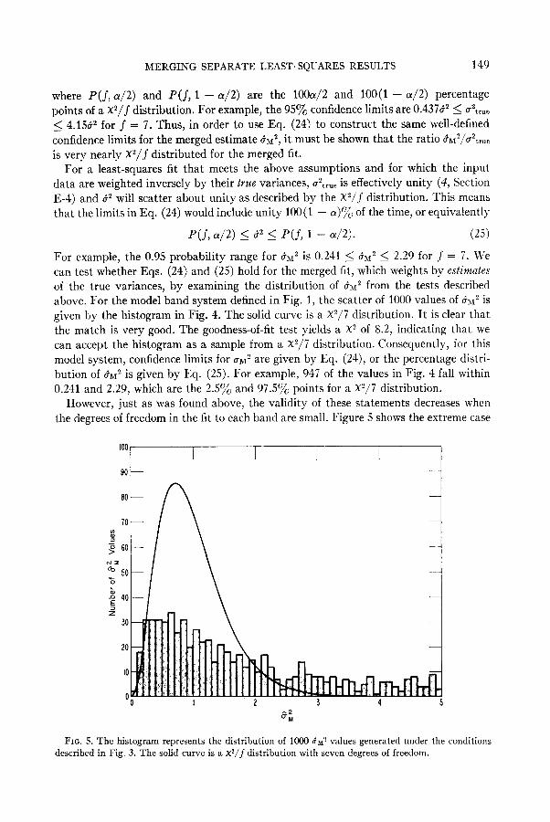
FIG. 5. The histogram represents the distribution of 1000 6~” values generated under the conditions described in Fig. 3. The solid curve is a x2/f distribution with seven degrees of freedom.
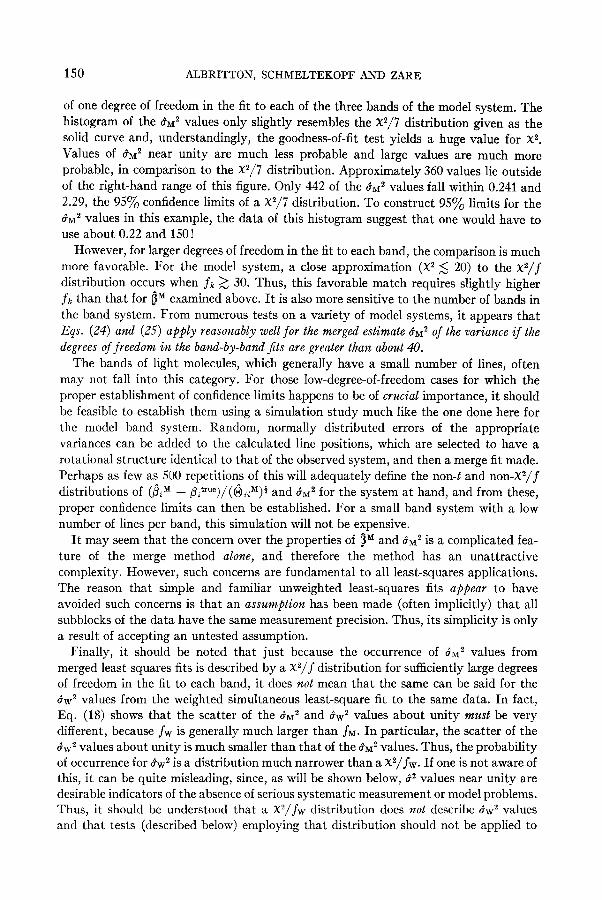
150 ALBRITTON, SCHMELTEKOPF AND ZARE
of one degree of freedom in the fit to each of the three bands of the model system. The histogram of the 6~~ values only slightly resembles the X2/7 distribution given as the solid curve and, understandingly, the goodness-of-fit test yields a huge value for ~2. Values of 8~~ near unity are much less probable and large values are much more
probable, in comparison to the X2/7 distribution. Approximately 360 values lie outside of the right-hand range of this figure. Only 442 of the 8~~ values fall within 0.241 and
2.29, the 95% confidence limits of a X2/7 distribution. To construct 95% limits for the 8~~ values in this example, the data of this histogram suggest that one would have to use about 0.22 and 1.50!
However, for larger degrees of freedom in the fit to each band, the comparison is much more favorable. For the model system, a close approximation (X2 ,< 20) to the x2/f distribution occurs when fk 2 30. Thus, this favorable match requires slightly higher
jk than that for @” examined above. It is also more sensitive to the number of bands in the band system. From numerous tests on a variety of model systems, it appears that
Eqs. (24) and (25) apply reasonably well for the merged estimate 8112~ of the variance if the
degrees of freedom in the band-by-band fits are greater than about 40.
The bands of light molecules, which generally have a small number of lines, often may not fall into this category. For those low-degree-of-freedom cases for which the
proper establishment of confidence limits happens to be of crucial importance, it should be feasible to establish them using a simulation study much like the one done here for the model band system. Random, normally distributed errors of the appropriate variances can be added to the calculated line positions, which are selected to have a
rotational structure identical to that of the observed system, and then a merge fit made. Perhaps as few as 500 repetitions of this will adequately define the non-t and non-X2/j distributions of (piM - P;true)/($iiM)+ and 8~~ for the system at hand, and from these,
proper confidence limits can then be established. For a small band system with a low number of lines per band, this simulation will not be expensive.
It may seem that the concern over the properties of 6” and 8~~ is a complicated fea-
ture of the merge method alone, and therefore the method has an unattractive complexity. However, such concerns are fundamental to all least-squares applications. The reason that simple and familiar unweighted least-squares fits appear to have avoided such concerns is that an assumption has been made (often implicitly) that all subblocks of the data have the same measurement precision. Thus, its simplicity is only
a result of accepting an untested assumption. Finally, it should be noted that just because the occurrence of 6~~ values from
merged least-squares fits is described by a X2/f distribution for sufficiently large degrees of freedom in the fit to each band, it does not mean that the same can be said for the dw2 values from the weighted simultaneous least-square fit to the same data. In fact, Eq. (18) shows that the scatter of the &r2 and Bw2 values about unity must be very different, because jw is generally much larger than Jo, In particular, the scatter of the Bw2 values about unity is much smaller than that of the 8~~ values. Thus, the probability of occurrence for Bw2 is a distribution much narrower than a X2/ fw. If one is not aware of this, it can be quite misleading, since, as will be shown below, 62 values near unity are desirable indicators of the absence of serious systematic measurement or model problems. Thus, it should be understood that a X’/~W distribution does psot describe SW” values and that tests (described below) employing that distribution should not be applied to
MERGING SEPARATE LEAST-SQUARES RESULTS 1.51
a &IV? value without the scaling implied by Eq. (18). These same remarks apply to
t-tests of @“(= @“) using hw = &+?b, since (B>\’ - flJrL’“)/(($i,w): does lzot follow a
t(fw) distribution, but rather a narrower distribution.
DETECTION OF RELATIVE !XSTEMATIC ERROR
The preceding section showed that, when the degrees of freedom of the fit to each
band are in the range of most spectroscopic applications, the merged variance Bxr” can be expected, with a chosen confidence, to lie in an asymmetric range about unity with limits given by the percentage points of the X’/jhl distribution, where jh~ are the degrees of freedom of the second step of the merged fit. This statement rests on the assumption of normally distributed measurement errors, which is frequently the case, and on the
assumption of no significant relatiz’e” systematic errors in either the measurements or the Hamiltonians used in fitting the measurements. This assumption, of course, often
can be very inappropriate. Any test that can indicate the presence of such relative systematic errors would be extremely valuable, since most statistical indicators gauge only random measurement error. As examples, it would be particularly useful to know whether relative systematic measurement errors exist in an extensive band system, where the wide wavelength range creates the strong possibility of such errors, or whether
undetected perturbations cause some of the Hamiltonians to be incomplete. We show in this section that such types of errors cause dh~~ to lie outside of the range expected for purely random errors and that this can be used as a convenient test for the likelihood
of their occurrence. To test the sensitivity of the test, the synthetic data methods described above were
used, except that various types of systematic errors were superimposed on the random errors. The first type of error considered is a constant 0.05 cm-’ shift in the wave- numbers of band 1 of the model system described in Fig. 1. For this electronic band,
therefore, the systematic shift is equal to one standard deviation of the random error. An error of this type is, of course, absorbed into and alters only the value of the origin
of the band. Thus, for the band-by-band results given in Table II, the only change is that v,,(O, 0) changes from 12 000.007(10) to 12 000.057(10) cm-‘. The former value missed the “true” value by 0.007 cm-’ due to the random errors. Now the latter value missed the “true” value by an additional 0.05 cm-’ due to the systematic error. Since the three bands are cyclically interrelated (see Fig. 111, this additional 0.05 cm-l will perturb the entire merge fit over and above that expected from random errors alone.”
Table VI shows the resulting merged constants. These should be compared to those in Table IV, which were determined without the systematic error. The values for 7’,,‘, R”‘, and Do are changed substantially, but the values for the other molecular constants are changed very little. This pattern can be understood in terms of the correlation coefficients. To’, which critically depends on the input value of ~~(0, 0), is rather strongly
I1 The discussion is limited to relutive systematic errors. An example would be an error that varied
systematically on wavelength. A ro~sfunt systematic error in ull of the measurements to be fitted is, of
course, undetectable by statistical tests.
I2 Such an error would loot extensively perturb a merged fit to a set of absorption bands with no com-
mon upper vibrational levels. Only the merged value for u0(0,0) would change. The reason is. of course, that there is no cyclic relation to any of the ~0 values of such a system.
152 ALBRITTON, SCHMELTEKOPFiAND ZARE
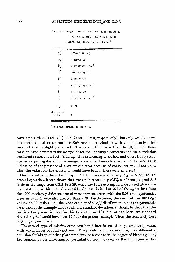
Table \'I. Merged Molecular Constants That Correspond
to the Band-By-Band Results in Table II
With vO(O,O) Increased by 0.05 cm -1
1?000.0248(160)
1.499979(66)
5.9878(258) x 10-6
2000.00054(209)
0.979981(46)
5.49?1(140) x 10-6
0.999982(46)
4.9923(140) x 10 -6
2.301
7
a Set the footnote of Table II.
correlated with Bo’ and Do’ (-0.515 and -0.500, respectively), but only weakly corre- lated with the other constants (0.069 maximum, which is with Tl”, the only other
constant that is slightly changed). The reason for this is that the (0, 0) vibration- rotation band dominates the merged fit for the unchanged constants and the correlation coefficients reflect this fact. Although it is interesting to see how and where this system- atic error propagates into the merged constants, these changes cannot be used as an indication of the presence of a systematic error because, of course, we would not know what the values for the constants would have been if there were no error!
Our interest is in the value of c?M = 2.301, or more particularly, 8~~ = 5.295. In the
preceding section, it was shown that one could reasonably (95% confidence) expect 8~1~ to lie in the range from 0.241 to 2.29, when the three assumptions discussed above are met. Not only is this one value outside of these limits, but 971 of the 8M2 values from
the 1000 randomly different sets of measurement errors with the 0.05 cm-’ systematic error in band 1 were also greater than 2.29. Furthermore, the mean of the 1000 6M2 values is 4.90, rather than the mean of unity of a x2/f distribution. Since the systematic error used in the example here is only one standard deviation, it should be clear that the test is a fairly sensitive one for this type of error. If the error had been two standard deviations, 8~~ would have been 17.6 for the present example. Thus, the sensitivity here is stronger than linear.
The second type of relative error considered here is one that systematically varies with wavenumber or rotational level. These could occur, for example, from differential emulsion shrinkage or other plate problems, or a change in the degree of blending along the branch, or an unrecognized perturbation not included in the Hamiltonian. We
MERGING SEPARATE LEAST-SQUARES RESULTS 15.3
simulate this type of error by introducing into the synthetic data of the (0,O) electronic band of the model system an error that linearly increases with wavenumber from zero
at the lowest wavenumber, with an average of 0.1 cm-’ (i.e., 2~). In the fit to these data,
k1 = 0.0528 cm-‘, hence is virtually unaffected by this type of relative systematic error and thus could give no indication of its presence, as it could if it had been several times
larger than the expected measurement precision. Furthermore, the largest change in the
estimated molecular constants was for Bo’ = 1.49981 cm-‘, which was a change of only
one standard error. Comparison of this value to the value obtained for this constant
from the (0, 1) electronic band would not indicate the possibility of an error. Thus, examination of the results of the band-by-band fits would not straightforwardly reveal
that anything was awry. However, the merged fit yields B&f2 = 2.18, which is outside of the range expected
with 9576 confidence from &I? when the errors are purely random. In fact, SO2 of the 1000 d-11” values obtained from the randomly different fits with this type of error were
larger than 2.29. The mean of these &f2 values was 2.49, rather than unity. Lastly, the effects of an error in the Hamiltonian of one of the bands were explored.
A realistic problem of this type would be whether or not to include the constant H,..
Values of H,, = 7 X lo-‘“, 6 X 10-12, and 5 X 10-l” cm-’ for ZZ,,‘, HI”, and Ho”,
respectively, were added to the “true” constants in Table I that were used to calculate the line positions of the three bands. For bands 1 and 3, H,’ and H,” were included in
the Hamiltonian used in the least-square fit to each band. However, for band 2, it was ~zot included. The repeated fits showed that this “model error” for band 2 produced 120 deleterious effects on either o”, h)“, or &‘. This is expected, of course, because these Ii,.
values cannot produce significant effects for the relatively lowJ lines of band 2. In this case, it should not matter whether H, is included or omitted in the Hamiltonian of the second band. Hence, while the equations given herein have been expressed in terms of one Hamiltonian for each vibrational level, it is not necessary in practice to include statis- tically insignificant constants.‘3
On the other hand, if the lines of band 2 are extended to include the first 50 R lines
and P lines and the “true” standard errors of the three bands are decreased by a factor of 10, the role of H, in band 2 becomes more important and the omission of Ho’ and ZZ1” from the Hamiltonian produces erroneous results. However, this is not immediately
obvious from the fit (without Ho’ and ZZ,‘) to band 2. For example, the other rotational
constants “absorb” the absence of ZZU’ and Hl” and $2 is virtually unharmed. In par-
ticular, the mean of the Bz values obtained from the 1000 fits to such sets of synthetic
data sets was 4.971 X lop3 cm-‘, which is very close to the “true” value. On the other
hand, a test least-squares fit to band 2 with El0 and H I” included would have suggested
their need. In addition, a careful comparison of the Bl” and &” values obtained from
band 2 without Ho’ and ZZl’, to those obtained separately from band 3, could probably
indicate that something was amiss. The point here is that a problem of some sort would
have been immediately obvious from the size of dM?. In the 1000 synthetic data fits,
la The statistically insignificant values from the band-bv-hand fits would have, of course, relatively
large standard errors, often many times larger than the fitied value of the constant. Since the square of
these standard errors are used as weights in the merged least-squares fit, the fitted values therefore have
negligible impact on the merged results. Of course, the covariances also play a role here.
154 ALBRITTON, SCHMELTEKOPF AND ZARE
985 of the 8~ values were larger than the 2.29 limit expected if all of the least-squares assumptions were valid. The mean 8~ value was 5.2.
These tests show that certain types of relative systematic errors cause the expected 61’ distribution to skew toward larger values. Thus, if a fitted 6M2 value for a particular set of laboratory data is larger than the upper value of a selected pair of confidence
limits, one rejects the hypothesis that the errors are randomly produced and considers the possibility of systematic problems.
The size of the confidence limits are, of course, a factor in this decision and reflect a
personal choice, in which one balances the desire to be specific against the fear of being wrong. The limits used above as examples corresponded to a 5% risk of erroneously concluding that something was wrong when in fact it was sot. Wider limits, say 0.141 and 2.90, would reduce the risk of this type of erroneous conclusion to l$&, but would, of course, increase the risk of failing to detect that something was wrong when in fact it was. Hamilton (11, pp. 45-49) provides an elaboration on this balance.
The merge fit of the model system has only seven degrees of freedom. Usually, spectroscopic band systems are more extensive than this model and the merged degrees
of freedom are much higher. For example, the application of the merged fit in the accompanying paper (6) has 95 degrees of freedom, for which the 95% confidence limits are much narrower, 0.74 and 1.31.
Of course, many other types of systematic errors can certainly occur. These examples suggest that the merged variance test should prove useful in indicating the presence of many of them. The test is, of course, blind to the exact location of the problem, but a
strong indication that a problem exists can provide the needed incentive for what is often a tedious rechecking. Finally, even though a recheck of the measurements or Hamiltonians does not discover the source of the problem, we feel that being aware of the existence of the problem is nevertheless valuable information. One would know, for
example, not to completely trust the statistical indicators, like standard errors and the
confidence limits derived from them. The extent to which the statistical meaning of spectroscopic standard errors is
damaged by the presence of relative systematic errors is an interesting and clearly worthwhile subject for general study, but is beyond the present scope. We only note here that jor the types and mapitudes of errors examined above, the confidence limits (Eq. (22b)) proved fairly reasonable; namely, the use of the fitted value c+M~, which is larger than normal because of the relative systematic errors, to compute GM (Eq. (8)), yields standard errorsI large enough to encompass the “true” value with roughly the proba- bility associated with the selected multiplicative t factor. However, this should only be taken to suggest that some of the usual meaning of the standard error still exists even
when moderate systematic errors are present. Without a detailed study, safety seems
to dictate that when the &M2 test indicates that moderate systematic errors are present,
somewhat more conservative confidence limits are desirable, e.g., from 99 to 99.99% limits
rather than the popular 95%. (This means standard deviation multiples from 2.5 to
3.9, respectively, rather than the popular 2.0, for high degrees of freedom.) Ramsey (12)
also discusses this point.
14 The increase of bnr2 due to relative systematic problems may, of course, entirely offset the improve- ment of precision associated with the decrease of ox when the merged data set is enlarged.
MERGING SEPARATE LEAST-SQUARES RESULTS 15.5
SUMMARY AND CONCLUSIONS
The two-step merged band-by-band method is a way to determine the most precise,
single values for the molecular constants of a system of n interconnected bands. Its first
step, defined by Eqs. (l)-(4), is the set of familiar band-by-band least-squares fits to the n bands of the system, the output quantities of which are the n = 1, 2,3, . . . sets of molecular constants ok and accompanying variance-covariance matrices 6)l~. These
quantities serve as input to the second step, defined by Eqs. (5)-(lo), which is a corre- lated least-squares fit that yields the minimum-variance single values 6” for the molec-
ular constants. The advantages offered by this method are as follows:
(1) The first step is one that is already commonly done in most two-state reduc- tions (see footnote 1) of a set of bands. However, one need not now stop at this point. The redundancy of most band systems can be utilized to obtain more precise estimates
of the molecular constants by storing the values’” @k and 6k from each of the final
band-by-band fits and using them as input to the merge fit. (2) It is not necessary to go back to the line position measurements and fit all of
them in a massive weighted simultaneous multiband fit (Eqs. (ll)-(15)). The merged
fit gives the equivalent results with much less data handling and computer storage requirements. However, the merged results are not equivalent to the unzoeighted simul- taneous multiband fit, which is less desirable because it makes the unnecessary (and often incorrect) assumption that all of the bands are of the same measurement precision.
(3) For most spectroscopic applications in which the degrees of freedom of the band-by-band fits are sizable (say, greater than about 40), the merged estimates @“‘,
hhf, and d&r2 have the usual statistical properties. This means that the standard errors (Gii”)f can be used to construct confidence limits for the estimates dihl (Eq. (22b)) that have their usual meaning. Similarly, confidence limits can be constructed for dlX2
(Eq. (25)). Thus, these limits can be used in the customary way for model testing, rejection of spurious measurements, etc.
(4) One of the more valuable of these tests is whether a fitted value C@ is reason- able. In particular, if it lies substantially outside of the confidence limits expected for
6~’ values whose variation about unity is due only to random measurement errors, then one can conclude that it is likely that relative systematic errors are present in some or all of the data sets or Hamiltonians.
(3) Although the merge method has been presented here in the context of reducing a band system to molecular constants, it is actually a very general method having much wider application within spectroscopy and elsewhere. A few other applications can be mentioned. The procedure obviously can merge the fitted results from investigations of all types: bands from different or the same electronic systems, vibration-rotation, micro- wave,lF Raman, etc. However, when the set of results to be merged are from more and more heterogeneous sources, problems may naturally arise; e.g., the 6,1, matrices may not be available and systematic measurement and Hamiltonian differences are much more likely. For example, such problems can make the treatment of all of the inter-
I5 In storing the values of i, and 6k, care must be taken to avoid the rounding off of digits that have relative significance (see Ref. (4), Sections G-l-d and G-2-a).
I6 One problem that might arise here is that least-squares fits to microwave data often have very low degrees of freedom.
156 ALBRITTON. SCHMELTEKOPF AND ZARE
connected data for a molecule, with the goal of obtaining the best single constants for all of the vibrational levels, a frustrating will-o’-the-wisp. A final noteworthy application is that the method can merge band-by-band results into, not just molecular constants,
but the best Dunham coefficients Yij (i.e., we, uexe, ueye, . . . , B,, a,, ye, . . .) for the data set, or any combination of molecular constants and Dunham coefficients. An example is given in the accompanying paper (6).
In conclusion, it should be clear that all possibilities and problems of the merged technique have not been explored here. However, enough has been done, hopefully, to
demonstrate the potential of the technique to (a) properly utilize the redundancy of a band system and (b) to indicate the presence of relative systematic errors in a data set, which are two common problems faced routinely in the fitting of models to spectroscopic
data.
ACKNOWLEDGMENTS
R. N. Zare gratefully acknowledges support of the National Science Foundation. We appreciate the comments and suggestions of Dr. J. A. Coxon and Dr. J. W. C. Johns on the manuscript.
RECEIVED: January 24, 1977
REFERENCES
1. D. L. ALBRITTON, W. J. HARROP, A. L. SCHYELTEXOPF, R. N. ZARE, AND E. L. CROW, J. Mol. Spectrosc. 46, 67 (1973).
2. N. &LUND, J. Mol. Spectrosc. 50, 424 (1974). 3. J. PL~VA AND W. B. TELFAIR, J. Mol. Spectrosc. 53, 221 (1974). 4. D. L. ALBRITTON, A. L. SCHMELTEKOPF, AND R. N. ZARE, An introduction to the least-squares fitting
of spectroscopic data in “Modern Spectroscopy, Modern Research II” (K. Narahari Rao, Ed.), pp. l-67, Academic Press, New York, 1976.
5. K. L. SAENGER, R. N. ZARE, AM) C. W. MATHEWS, J. Mol. Spectrosc. 61, 216 (1976). 6. D. L. ALBRITTON, A. L. SCHULTEKOPF, W. J. HARROP, R. N. ZARE, AND J. CZARNY, J. Mol.
Spectrosc. 67, 157-184. (1977). 7. W. H. KIRCHHOFF, J. Mol. Spectrosc. 41, 333 (1972). 8. G. HERZBERG, “Spectra of Diatomic Molecules,” p. 103. Van Nostrand, New York, 1950. 9. S. R. SEARLE, “Linear Models,” Wiley, New York, 1971.
10. W. J. DIXON AND F. J. MASSEY, “Introduction to Statistical Analysis,” 3rd. ed., McGraw-Hill,
New York, 1969. Il. W. C. HAMILTON, “Statistics in Physical Science,” Ronald Press, New York, 1964. 12. D. A. RAYSAY, Critical evaluation of molecular constants from optical spectra, in “Critical Evalua-
tion of Chemical and Physical Structural Information,” Proceedings of a Conference at Dartmouth
College, June 24-29, 1973 (D. R. Lide, Jr. and M. A. Paul, Eds.), pp. 116129, National Academy of Sciences, Washington, D. C., 1974.