A METHOD FOR INITIALIZATION OF ENSEMBLE DATA ASSIMILATION

Milija Zupanski1, Steven Fletcher1, I. Michael Navon2, Bahri Uzunoglu3,

Ross P. Heikes4, David A. Randall4, and Todd D. Ringler4

Submitted January 2005

(6 Figures)

A manuscript submitted for publication to

Tellus 1 Cooperative Institute for Research in the Atmosphere Colorado State University 1375 Campus Delivery Fort Collins, CO 80523-1375 2 Department of Mathematics and

School of Computational Science and Information Technology Dirac Science Library Building Florida State University Tallahassee, FL 32306-4120

3 School of Computational Science and Information Technology

Dirac Science Library Building Florida State University Tallahassee, FL 32306-4120

4 Department of Atmospheric Science Colorado State University 1371 Campus Delivery Fort Collins, CO 80523-1371

1

Abstract

The initialization of ensemble perturbations at the beginning of ensemble data

assimilation is addressed. The presented work examines the impact of initialization in the

Maximum Likelihood Ensemble Filter (MLEF) framework, but it is applicable to other

ensemble data assimilation algorithms as well.

An empirical method of creating the initial ensemble perturbations is proposed,

based on the use of the Kardar-Parisi-Zhang (KPZ) equation to form sparse random

perturbations, followed by a spatial smoothing to enforce desired correlation structure.

The proposed method is by design simple and computationally efficient.

Data assimilation experiments are conducted using a global shallow-water model

and simulated observations. The proposed correlated-KPZ method is compared to the

commonly used method of uncorrelated random perturbations. The results indicate that

the impact of the correlated-KPZ ensemble initialization is beneficial. The root-mean-

square error rate of convergence of data assimilation is improved, and the positive impact

is noticeable throughout the data assimilation cycles. The sensitivity to the choice of the

correlation length scale exists, although it is not very high. The implied computational

savings and improvement of the results may be important in future realistic applications

of ensemble data assimilation.

2

1. Introduction

Ensemble data assimilation is a fast developing methodology designed to address

the probabilistic aspect of prediction and analysis. It lends itself as a bridge between

relatively independently developed data assimilation and ensemble forecasting

methodologies. Beginning with the pioneering work of Evensen (1994), followed by

Houtekamer and Mitchell (1998), there are now many ensemble data assimilation

algorithms (Pham et al. 1998; Lermusiaux and Robinson 1999; Brasseur et al. 2000;

Keppenne 2000; Bishop et al. 2001; Anderson 2001; Van Leeuwen 2001; Whitaker and

Hamill 2002; Reichle et al. 2002a; Anderson 2003; Snyder and Zhang 2003; Ott et al.

2004; Zupanski 2005; Zupanski and Zupanski 2005). Realistic applications with the state-

of-the-art models and real observations are also intensively pursued in recent years

(Houtekamer and Mitchell 2001; Keppene and Rienecker 2002; Haugen and Evensen

2002; Szunyogh et al. 2005).

One of the remaining issues, rarely addressed in literature, is the initiation of an

ensemble data assimilation algorithm. Ideally, the initial ensemble perturbations should

represent the error statistics of the model state. In practice, the error statistics is measured

by the error covariance. It is known that the error covariance has a structure, in principle

defined by model dynamics, and formally represented by correlations between model

variables. In particular, one would like to create initial perturbations reflecting the

structure of the error covariance.

A common practice used to initiate an ensemble data assimilation algorithm is to

form uncorrelated random initial fields, sampled from a probability distribution, and then

use them as initial perturbations in ensemble forecasting step of ensemble data

assimilation algorithm. An obvious problem with this approach is that the analysis error

covariance does not have any correlations between variables. In order to improve the

correlation structure in the initial ensemble, Dowell et al. (2004) and Zhang et al. (2004)

use prescribed ellipsoidal perturbations, with randomly chosen locations in the vicinity of

the observation locations. Another approach, described by Evensen (2003), also

recognizes the need for correlation structure in initial ensemble perturbations. The

approach is based on the use of Fourier representation of the perturbations, effectively

3

representing a prescribed correlation structure of the analysis error covariance. A random

number generator is used to create random phase shifts.

We propose a new method for creating initial ensembles. The method begins by

employing the Kardar-Parisi-Zhang (KPZ) equation, followed by forcing of the

correlations at a preferred length scale. As the methods of Evensen (2003) and Dowell et

al. (2004), the proposed method is empirical, in the sense that some previous knowledge

about the analysis/forecast error covariance is assumed, used to define a typical variance

and a typical decorrelation length for each control variable. The proposed method differs

from the above mentioned methods, however, since it does not assume any particular

form of perturbations (e.g., wave-like, or ellipsoidal), nor the location of random

perturbations. This should make the method more robust and suitable for realistic model

applications, where the perturbations have an unknown, seemingly random form.

The proposed method is evaluated within the Maximum Likelihood Ensemble

Filter (MLEF – Zupanski 2005) framework. However, the method is directly applicable

to other ensemble data assimilation algorithms as well. The methodology will be

explained in Section 2, experimental design will be presented in Section 3, results in

Section 4, and conclusions will be drawn in Section 5.

2. Correlated-Kardar-Parisi-Zhang equation method

2.1. The problem

The initial step of an ensemble data assimilation algorithm is usually the ensemble

forecasting. Since in this work the MLEF algorithm (Zupanski 2005) is used, let the

square-root forecast error covariance be defined as

( ) )1()()( 1121

1/2 k-ai

k-aiSf MM xpxbbbbP −+=⋅⋅=

where Pf is the forecast error covariance at time tk (e.g., current analysis time), defined

over the ensemble-spanned subspace, S is the number of ensemble perturbations, M is the

nonlinear forecast model integrated from time tk-1 to time tk, bi are the columns of the

4

square-root forecast error covariance, pi are the columns of the square-root analysis error

covariance, and xa is the previous analysis at time tk-1. The problem we address is the

initiation of the ensemble perturbations at the very beginning of data assimilation, i.e. the

specification of the initial column vectors pi. Note that at later stages of data

assimilation, the square-root analysis error covariance columns are calculated by data

assimilation algorithm.

There are two important practical issues in initiating an ensemble forecast. One is

that the initial ensemble perturbations pi need to have an inherent randomness, reflecting

the fact that the magnitude and location of unstable initial perturbations is not known a

priori. Second issue is that a correlation structure in the initial perturbations is desired,

since the outer product of perturbation vectors forms the analysis error covariance.

Matching these two requirements may not be simple, due to the additional restriction

imposed by the ensemble size.

2.2. The method

Since we anticipate smoothing of initially uncorrelated random perturbations, we

would like first to create random perturbations with spatially sparse (e.g., distant), large

amplitude peaks, i.e. we wish to form sparse uncorrelated random patterns. The

consequent smoothing of these uncorrelated random patterns should impose a prescribed

length scale on perturbations, ultimately creating correlated random patterns. In order to

create the uncorrelated random patterns, the Kardar-Parisi-Zhang (KPZ) equation will be

used (Kardar et al. 1986; Beccaria and Curci 1994; Newman and Bray 1996; Maunuksela

et al. 1999; Marinari et al. 2002) in the one-dimensional form

)2()( 22 ξ+∇+∇=∂∂ hhh

t

where h is the perturbation vector and ξ is a random forcing vector, in our application a

white Gaussian random noise with unit variance. This equation is used to explain the

dynamics of interfaces moving through random media. Our interest in this equation

comes from the relation of the KPZ class of equations to dynamic localization of

5

Lyapunov vectors. As suggested by Pikovsky and Politi (1998) the Lyapunov vector is

the exponential of the roughened interface, and thus can be represented by the KPZ

equation, which models the dynamics of rough interfaces. The mentioned connection

between the dynamics of roughening interfaces and the Lyapunov vectors is, in fact, used

to explain the observed spatial and temporal localization of the Lyapunov vectors. The

consequence is that the KPZ equation can be used to create sparse uncorrelated random

perturbations, fitting well our first task.

The next task is to force the correlations between the patterns to a preferred length

scale. This is done by applying a spatially localized correlation function to each of the

perturbation vectors. After doing so, the ensemble perturbations are smooth, dominated

by the correlations at the scales defined by the imposed correlation function.

Note that there is an important dependence between the sparseness of the

uncorrelated random patterns and the imposed correlation length scale: the average

distance between the uncorrelated random amplitude peaks (i.e. the sparseness of the

random patterns) should correspond to the correlation length scale. This requirement

assures that the non-zero perturbations are defined over the full integration domain.

-1.00E+00

-5.00E-01

0.00E+00

5.00E-01

1.00E+00

1 11 21 31 41 51 61 71 81 91Am

plitu

de

original KPZcorrelated-KPZ

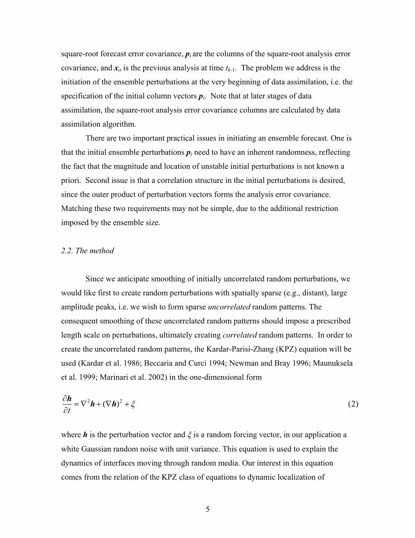
Fig.1. A perturbation vector obtained after integrating the KPZ equation over 200 non-dimensional time steps: (a) without imposed correlations (solid line), and (b) with an imposed correlation with the length scale of 5 non-dimensional units (dotted line). The one-dimensional integration domain contains 100 grid points.

6

A typical result of the one-dimensional integration of Eq. (1) is shown in Fig.1.

One can note uncorrelated random perturbations at each grid-point, with only few

dominating peaks, thus indicating a spatially localized pattern. The sparseness of these

patterns is what we are looking for. The impact of the correlation imposed on the KPZ

random perturbation is seen as a smooth dotted line in Fig.1. The created smooth line

represents a correlated random perturbation that would be used as an initial ensemble

perturbation.

2.3. Algorithmic details

In practice, the correlated-KPZ methodology is applied in non-dimensional space,

and only at the end the resulting correlated random perturbations are multiplied by a

prescribed forecast error standard deviation. Note that the sparseness of the uncorrelated

random patterns depend on the length of time integration of the KPZ equation: the longer

integration, the sparser the patterns. This empirical relation is used in this algorithm

)3(_ scalelengthtime ⋅= α

where time refers to the number of the time steps of the KPZ equation, length_scale is a

prescribed correlation length-scale, and a is an empirical parameter (in our application

α=0.2).

When applying the KPZ equation in discrete form, a simple centered finite

differencing is used for spatial derivatives, and the one-level forward scheme for time

integration (e.g., Haltiner and Williams 1980). The algorithmic steps are as follows:

(i) Given the correlation length scale, use Eq.(3) to define the number of time

steps for the KPZ equation integration.

(ii) Integrate the one-dimensional KPZ equation along main spatial axes. Use

the uncorrelated random perturbations ξ from a specific probability

distribution (e.g., white Gaussian N(0,1) distribution in this case).

Renormalize h (if needed) by imposing an upper limit |h| ≤Nσ, where σ is

the standard deviation (σ=1 and N=3 in this case).

7

(iii) Apply a spatially-localized, compactly-supported function to each non-

dimensional perturbation.

(iv) Form initial ensemble perturbations by multiplying with prescribed

standard deviation.

3. Experimental design

In this section few basic experiments are defined in order to illustrate the impact

of the choice of initial perturbations on ensemble data assimilation. The correlation

function used in creating correlated random noise is a compactly-supported space-limited

Second Order Auto-Regressive (SOAR) correlation function (Gaspari and Cohn 1999,

Eq. (4.4)). As mentioned earlier, the MLEF methodology (Zupanski 2005) is used in all

experiments.

3.1. Model

A finite-difference shallow-water model developed at the Colorado State

University is used in this study (Heikes and Randall 1995a,b). This is a global model,

constructed on a twisted icosahedral grid. The grid consists of hexagons and pentagons,

effectively reducing the pole problem. The prognostic variables are height, velocity

potential, and stream function. The time integration scheme is the third-order Adams-

Bashforth scheme (Durran 1991). The model was successfully tested on the suite of seven

test cases described by Williamson et al. (1992) (e.g., Heikes and Randall 1995a). The

number of grid cells used in this study is 2562, which corresponds to the model resolution

of approximately 4.5 degrees of longitude-latitude.

3.2. Observations

The observations are created by adding random Gaussian perturbations to a model

forecast, which we refer to as a truth. This implies a perfect model assumption. Although

the model equations formally predict the velocity potential and the stream function, more

8

conventional wind observations are created, and later assimilated. The observation error

covariance R is assumed diagonal, i.e. no correlation between observations is assumed.

The observation error chosen for the height is 5 m, and for the wind is 0.5 ms-1. There

are overall 1025 randomly chosen observations in each analysis cycle. These

observations consist of approximately 500 height observations, and 500 wind

observations. The wind observations are equally divided between the east-west and north-

south wind components. The observations are assimilated every six hours.

3.3. Experiments

The initial conditions are defined from the test case 5 of Williamson et al. (1992),

which corresponds to a geostrophically-balanced zonal flow over an isolated conical

mountain. The initial zonal flow is 20 ms-1, and the mountain is centered at 300N, 900W,

with the height of 2000 m. This set-up is characterized by the excitation of Rossby and

gravity waves, with notable nonlinearity occurring in the vicinity of the mountain.

In all experiments there are 1000 ensemble members used. Total number of

degrees of freedom is 12,800. Such high number is not necessarily needed, but it helps in

relaxing the impact of degrees of freedom, thus allowing a more focused examination of

the ensemble initialization. The observations are defined at model grid-points, implying

the linearity of the observation operator. The assimilation is performed over 15 days,

which corresponds to 60 data assimilation cycles of 6-hour intervals. The initial

conditions for the experimental run are defined same as in the forecast run used to create

observations (e.g., the test case 5), however initiated 6 hours earlier in order to create

erroneous initial conditions. The initial forecast error covariance has a standard deviation

about two times larger than the observation error (i.e. 10 m for height and 1 ms-1 for

winds), which is considered to be realistic.

The experiments are separated in two groups: (i) the correlated-KPZ method is

compared with the uncorrelated random perturbation method, and (ii) the sensitivity of

the analysis to the correlation length scale in the correlated-KPZ method is evaluated.

The results are compared using the root-mean-square (RMS) analysis error,

defined as a difference between the analysis and the truth (e.g., the forecast used to create

9

observations), valid at the time of the analysis. In addition, the χ2-test (e.g., Menard et al.

2000), and the rank histogram of normalized innovation vectors (e.g., observation minus

guess) (Reichle et al. 2002b; Zupanski 2005), are also used.

4. Results

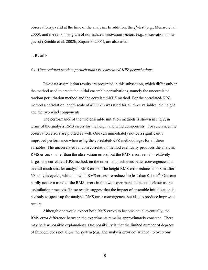
4.1. Uncorrelated random perturbations vs. correlated-KPZ perturbations

Two data assimilation results are presented in this subsection, which differ only in

the method used to create the initial ensemble perturbations, namely the uncorrelated

random perturbation method and the correlated-KPZ method. For the correlated-KPZ

method a correlation length scale of 4000 km was used for all three variables, the height

and the two wind components.

The performance of the two ensemble initiation methods is shown in Fig.2, in

terms of the analysis RMS errors for the height and wind components. For reference, the

observation errors are plotted as well. One can immediately notice a significantly

improved performance when using the correlated-KPZ methodology, for all three

variables. The uncorrelated random correlation method eventually produces the analysis

RMS errors smaller than the observation errors, but the RMS errors remain relatively

large. The correlated-KPZ method, on the other hand, achieves better convergence and

overall much smaller analysis RMS errors. The height RMS error reduces to 0.8 m after

60 analysis cycles, while the wind RMS errors are reduced to less than 0.1 ms-1. One can

hardly notice a trend of the RMS errors in the two experiments to become closer as the

assimilation proceeds. These results suggest that the impact of ensemble initialization is

not only to speed-up the analysis RMS error convergence, but also to produce improved

results.

Although one would expect both RMS errors to become equal eventually, the

RMS error difference between the experiments remains approximately constant. There

may be few possible explanations. One possibility is that the limited number of degrees

of freedom does not allow the system (e.g., the analysis error covariance) to overcome

10

0.0

5.0

10.0

15.0

20.0

1 11 21 31 41 51

Analysis cycle

RMS

erro

r (m

)

obs errorrandomkpz

(a) (b)

0.0

0.5

1.0

1.5

2.0

1 11 21 31 41 51

Analysis cycle

RMS

erro

r (m

/s)

obs errorrandomkpz

(c)

0.0

0.5

1.0

1.5

2.0

1 11 21 31 41 51

Analysis cycle

RMS

erro

r (m

/s)

obs errorrandomkpz

Fig. 2. Analysis RMS error for: (a) height (m), (b) east-west wind component (ms-1), and (c) north-south wind component (ms-1). The results are obtained using: (i) uncorrelated random perturbations (thin full line) method, and (ii) correlated-KPZ method (thick full line) method. The observation error standard deviation is indicated by a dotted line.

11

noisy initial perturbations created by the uncorrelated random perturbation method.

Another possible explanation is that the assimilation period of 6 hours may not be long

enough to allow the initial, noisy forecast error covariance to become smooth. Also, the

information collected from observations may not be dense enough to impact all grid

points, due to the shorter correlation lengths. All these possible scenarios are only made

worse due to the computer round-off errors, accumulated over many assimilation cycles.

Although important, a full understanding of such behavior of RMS errors does require a

detailed investigation, thus it is left for future.

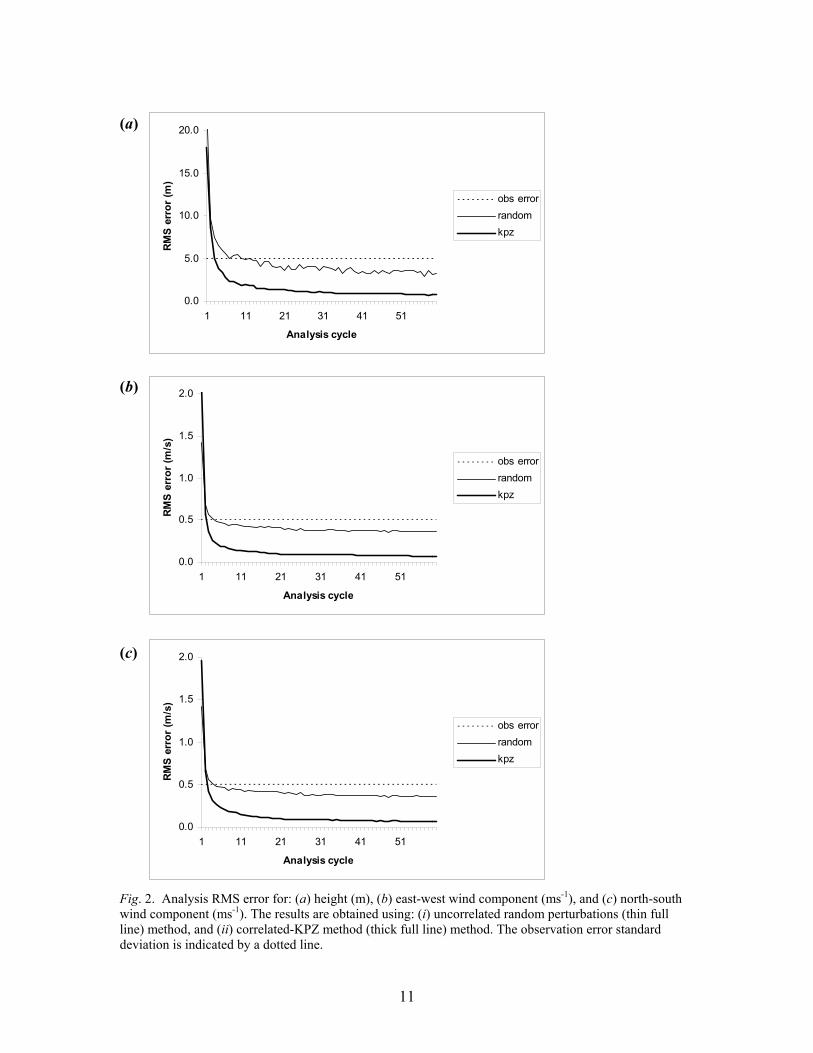
In terms of the normalized innovation vector statistics, the correlated-KPZ

method again shows an improved performance (Figs.3 and 4). The optimal value for the

χ2-test is one. Results in Fig.3 indicate large deviations from the optimal value in the

uncorrelated random perturbation experiment, eventually settling in the 1.2-1.3 range. On

the other hand, the results of the correlated-KPZ experiment show much better values,

closer to one.

0.00E+00

5.00E-01

1.00E+00

1.50E+00

2.00E+00

1 11 21 31 41 51

Cycle

chi-s

quar

e

kpzrandom

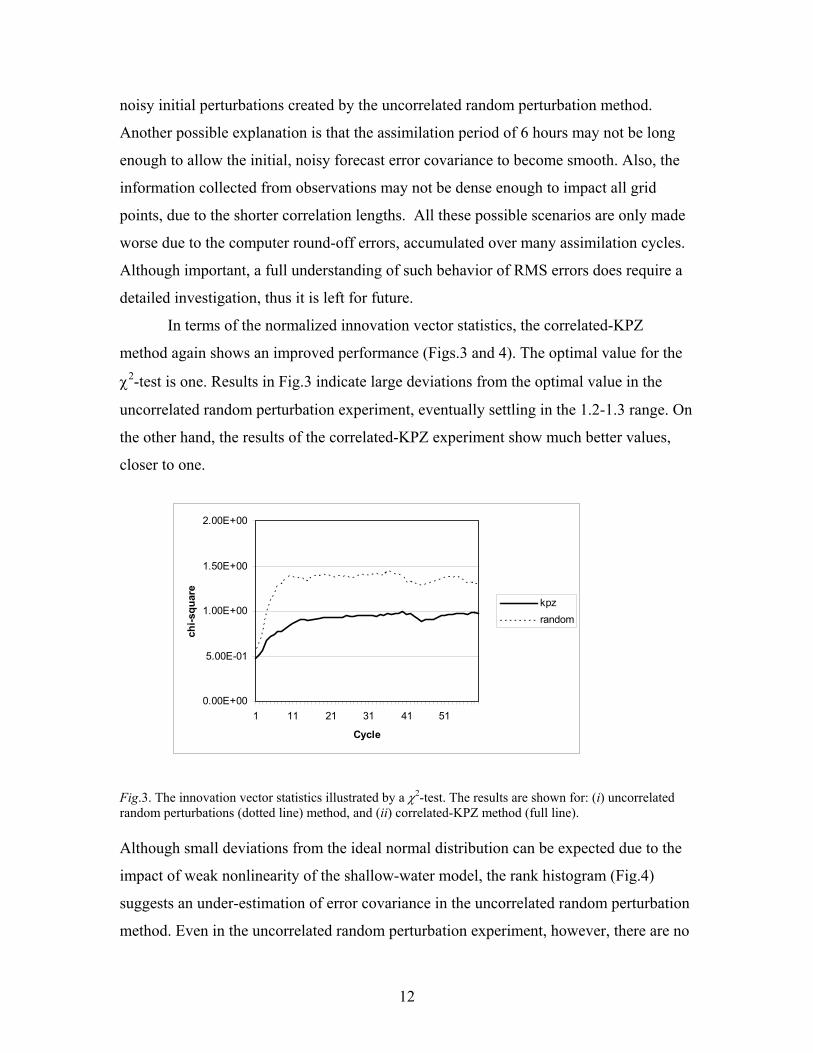
Fig.3. The innovation vector statistics illustrated by a χ2-test. The results are shown for: (i) uncorrelated random perturbations (dotted line) method, and (ii) correlated-KPZ method (full line). Although small deviations from the ideal normal distribution can be expected due to the

impact of weak nonlinearity of the shallow-water model, the rank histogram (Fig.4)

suggests an under-estimation of error covariance in the uncorrelated random perturbation

method. Even in the uncorrelated random perturbation experiment, however, there are no

12

outliers, meaning that ensembles are adequately covering the necessary range of

perturbations (e.g., ensemble spread is adequate). Overall, the innovation vector statistics

indicates a stable performance of the MLEF algorithm in both ensemble initiation

experiments. (a)

0.00E+00

1.00E-01

2.00E-01

3.00E-01

4.00E-01

5.00E-01

-5 -4 -3 -2 -1 0 1 2 3 4 5

Normalized innovations

Rela

tive

frequ

ency

0.00E+00

1.00E-01

2.00E-01

3.00E-01

4.00E-01

5.00E-01

-5 -4 -3 -2 -1 0 1 2 3 4 5

Normalized innovations

Rela

tive

frequ

ency

(b) Fig.4. The innovation vector statistics illustrated by a rank histogram of normalized innovations. The results are obtained using: (a) uncorrelated random perturbations method, and (b) correlated-KPZ method.

13

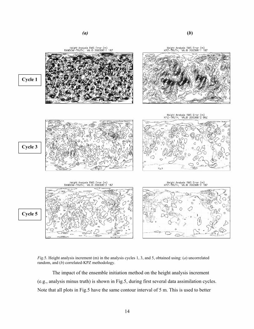
(a) (b)

(b)

Cycle 1

Cycle 3

Cycle 5

Fig.5. Height analysis increment (m) in the analysis cycles 1, 3, and 5, obtained using: (a) uncorrelated random, and (b) correlated-KPZ methodology.

The impact of the ensemble initiation method on the height analysis increment

(e.g., analysis minus truth) is shown in Fig.5, during first several data assimilation cycles.

Note that all plots in Fig.5 have the same contour interval of 5 m. This is used to better

14

illustrate a dramatic reduction of the analysis error. It is clear that the correlated-KPZ

experiment produces much smoother analysis increments, eventually resulting in superior

performance. By cycle 5, the height analysis increments in correlated-KPZ experiment

(Fig.5.b) are generally smaller than 5 m, with only few small areas with about 10 m. On

the other side, the analysis increments in the uncorrelated random initial perturbation

experiment (Fig.5.a) are quite noisy, especially in the cycle 1. Nevertheless, it appears

that the analysis increment noise is dramatically reduced in both experiments, suggesting

the robustness of the data assimilation algorithm.

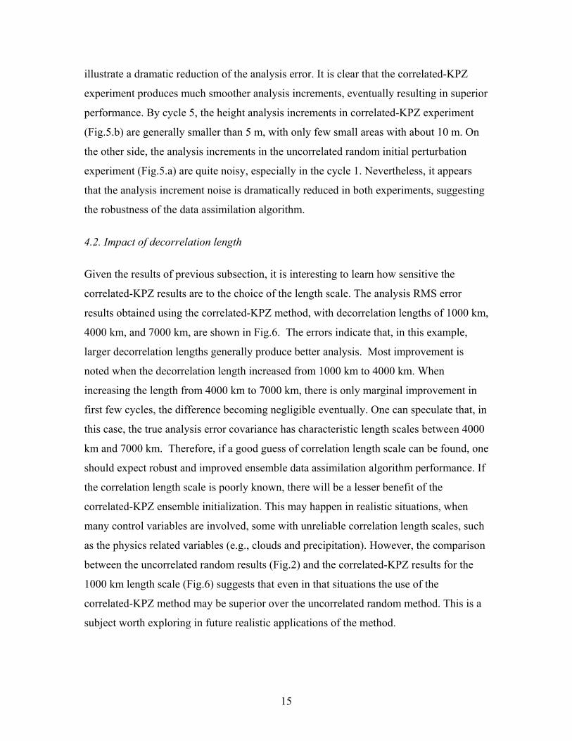
4.2. Impact of decorrelation length

Given the results of previous subsection, it is interesting to learn how sensitive the

correlated-KPZ results are to the choice of the length scale. The analysis RMS error

results obtained using the correlated-KPZ method, with decorrelation lengths of 1000 km,

4000 km, and 7000 km, are shown in Fig.6. The errors indicate that, in this example,

larger decorrelation lengths generally produce better analysis. Most improvement is

noted when the decorrelation length increased from 1000 km to 4000 km. When

increasing the length from 4000 km to 7000 km, there is only marginal improvement in

first few cycles, the difference becoming negligible eventually. One can speculate that, in

this case, the true analysis error covariance has characteristic length scales between 4000

km and 7000 km. Therefore, if a good guess of correlation length scale can be found, one

should expect robust and improved ensemble data assimilation algorithm performance. If

the correlation length scale is poorly known, there will be a lesser benefit of the

correlated-KPZ ensemble initialization. This may happen in realistic situations, when

many control variables are involved, some with unreliable correlation length scales, such

as the physics related variables (e.g., clouds and precipitation). However, the comparison

between the uncorrelated random results (Fig.2) and the correlated-KPZ results for the

1000 km length scale (Fig.6) suggests that even in that situations the use of the

correlated-KPZ method may be superior over the uncorrelated random method. This is a

subject worth exploring in future realistic applications of the method.

15

(a)

0.0

5.0

10.0

15.0

20.0

1 6 11 16 21 26

Analysis cycle

RMS

erro

r (m

)1000km4000km7000km

(b)

0.0

0.5

1.0

1.5

2.0

1 6 11 16 21 26

Analysis cycle

RMS

erro

r (m

/s)

1000km4000km7000km

(c)

0.0

0.5

1.0

1.5

2.0

1 6 11 16 21 26

Analysis cycle

RMS

erro

r (m

/s)

1000km4000km7000km

Fig.6. Sensitvity of the analysis RMS errors to decorrelation length in the correlated-KPZ method, for: (a) height (m), (b) east-west wind component (ms-1), and (c) north-south wind component (ms-1). Shown results are for decorrelation lengths of: (i) 1000 km (dotted line), (ii) 4000 km (thick full line), and (iii) 7000 km (thin full line). The results with decorrelation length of 4000 km are same as shown in Fig.2 for the correlated-KPZ results.

16

5. Summary and Conclusions

An empirical method for initiating the ensemble forecasts in the ensemble data

assimilation, named the correlated-KPZ method, is presented. In principle, empirical

methods should be applied when some experience with a particular model, and its

covariance structure exists. The correlated-KPZ method consists of two steps: (i)

creating sparse random perturbations using the KPZ equation, and (ii) imposing

correlations of a chosen length scale on the perturbations. The implication is that the

initial analysis error covariance is more realistic, thus enabling the ensemble data

assimilation to perform better, and achieve faster convergence in terms of the analysis

RMS error. The assimilation algorithm employed in the study is the MLEF, applied to

assimilation of simulated observations using a global shallow-water model. The

correlated-KPZ method is directly applicable to other ensemble data assimilation

algorithms.

Results indicate a superior performance of the correlated-KPZ method

over the uncorrelated random perturbation method. This is confirmed by the analysis

RMS scores, as well as by the innovation vector statistics. Sensitivity of the correlated-

KPZ method to the input correlation length parameter is relatively small, unless the

correlation length scale is poorly known, thus it is advantageous to have a good estimate

of the analysis error correlation length scale.

Overall results indicate that the ensemble initialization is an important component

of an ensemble data assimilation algorithm. In near future complex atmospheric models

will be used, in order to further evaluate the practicality of the proposed correlated-KPZ

method. Some variables, such as pressure, temperature and winds may have better known

correlation statistics than microphysical variables, such as clouds and precipitation. Then,

an important question is how difficult is to achieve an improvement in the context of

multiple control variables with poorly known correlation statistics. A possible

improvement of the method may be achieved by using the formulation of the KPZ

equation with spatially correlated noise (e.g., Janssen et al. 1999), such that the two

algorithmic steps collapse into just one step. This is more appealing from the

mathematical, as well as from the practical applications point of view, since the method

17

would become algorithmically simpler. Focused research of ensemble initialization

methods will eventually lead to more robust ensemble data assimilation algorithms,

important for future realistic applications.

18

Acknowledgments

We would like to thank Dusanka Zupanski for many helpful discussions and

careful reading of the manuscript. Our gratitude is also extended to the National Center

for Atmospheric Research, which is sponsored by the National Science Foundation, for

the computing time used in this research. This work was supported by the National

Science Foundation Collaboration in Mathematical Geosciences grant 0327651.

19

References Anderson, J. L. 2001: An ensemble adjustment Kalman filter for data assimilation. Mon.

Wea. Rev., 129, 2884-2903. Anderson, J. L. 2003: A local least squares framework for ensemble filtering. Mon.

Wea. Rev., 131, 634-642. Beccaria, M. and Curci, G. 1994: Numerical simulation of the Kardar-Parisi-Zhang equation. Phys. Rev. E, 50, 4560-4563. Bishop, B., Etherton, J. and Majmudar, S. J. 2001: Adaptive sampling with the ensemble

transform Kalman filter. Part I: Theoretical aspects. Mon. Wea. Rev., 129, 420-436.

Brasseur, P., Ballabrera, J. and Verron, J. 1999: Assimilation of altimetric data in the mid-latitude oceans using the SEEK filter with an eddy-resolving primitive equation model. J. Marine Sys., 22, 269-294.

Dowell, D. C., Zhang, F., Wicker, L. J., Snyder, C. and Crook, N. A. 2005: Wind and Temperature Retrievals in the 17 May 1981 Arcadia, Oklahoma, Supercell: Ensemble Kalman Filter Experiments. Mon. Wea. Rev., 132, 1982-2005.

Durran, D. R. 1991: The third-order Adams-Bashforth method: An attractive alternative to leapfrog time differencing. Mon. Wea. Rev., 119, 702-720. Evensen, G. 1994: Sequential data assimilation with a nonlinear quasi-geostrophic model

using Monte-Carlo methods to forecast error statistics. J. Geophys. Res., 99 (C5), 10 143-10 162.

Evensen, G. 2003: The Ensemble Kalman Filter: theoretical formulation and practical implementation. Ocean Dynamics, 53, 343-367. Gaspari, G. and Cohn, S. E. 1999: Construction of correlation functions in two and three

dimensions. Quart. J. Roy. Meteor. Soc., 125, 723-757. Haltiner, G. J. and Williams, R. T. 1980: Numerical Prediction and Dynamic Meteorology. Second ed., Wiley & Sons, 477 pp. Haugen, V. E. J. and Evensen, G. 2002: Assimilation of SLA and SST data into an

OGCM for the Indian Ocean. Ocean Dyn., 52, 133-151. Heikes, R. and Randall, D. A. 1995a: Numerical integration of the shallow-water

equations on a twisted icosahedral grid. Part I: Basic design and results of tests. Mon. Wea. Rev., 123, 1862-1880.

Heikes, R. and Randall, D. A. 1995b: Numerical integration of the shallow-water equations on a twisted icosahedral grid. Part II: Detailed description of the grid and an analysis of numerical accuracy. Mon. Wea. Rev., 123, 1881-1887.

Houtekamer, P. L. and Mitchell, H. L. 1998: Data assimilation using ensemble Kalman filter technique. Mon. Wea. Rev., 126, 796-811.

Houtekamer, P.L. and Mitchell, H. L. 2001: A sequential ensemble Kalman filter for atmospheric data assimilation. Mon. Wea. Rev., 129, 123-137.

Janssen, H. K., Tauber, U. C. and Frey, E. 1999: Exact results for the Kardar-Parisi- Zhang equation with spatially correlated noise. Eur. Phys. J. B, 9, 491-511. Kardar, M., Parisi, G. and Zhang, Y. C. 1986: Phys. Rev. Lett., 56, 889. Keppenne, C. L. 2000: Data assimilation into a primitive-equation model with a parallel

ensemble Kalman filter. Mon. Wea. Rev., 128, 1971-1981. Keppenne, C. L. and Rienecker, M. M. 2002: Initial testing of massively-parallel

20

ensemble Kalman filter with the Poseidon isopycnal ocean general circulation model. Mon. Wea. Rev., 130, 2951-2965.

Lermusiaux, P. F. J. and Robinson, A. R. 1999: Data assimilation via error subspace statistical estimation. Part I: Theory and schemes. Mon. Wea. Rev., 127, 1385-1407.

Marinari, E., Pagnani, A., Parisi, G. and Racz, Z. 2002: Width distributions and the upper critical dimension of Karadar-Parisi-Zhang interfaces. Phys. Rev. E, 65, 026136. Maunuksela, J., Myllys, M., Timonen, J., Alava, M. J. and Ala-Nissila, T. 1999: Kardar- Parisi-Zhang scaling in kinetic roughening of fire fronts. Physica A, 266, 372-376. Menard, R., Cohn, S. E., Chang, L.-P. and Lyster, P. M. 2000: Assimilation of

stratospheric chemical tracer observations using a Kalman filter. Part I: Formulation. Kalman filter. Mon. Wea. Rev., 128, 2654-2671.

Newman, T. J. and Bray, A. J. 1996: Strong-coupling behaviour in discrete Kardar-Parisi- Zhang equations. J. Phys. A., 29, 7917-7928. Ott, E., Hunt, B. R., Szunyogh, I., Zimin, A. V., Kostelich, E. J., Corazza, M., Kalnay,

E., Patil, D. J. and Yorke, J. A. 2004: A Local Ensemble Kalman Filter for Atmospheric Data Assimilation. Tellus, 56A, No. 4, 273-277.

Pham, D. T., Verron, J. and Roubaud, M. C. 1998: A singular evolutive extended Kalman filter for data assimilation in oceanography. J. Marine Sys., 16, 323-340.

Pikovsky, A. and Politi, A. 1998: Dynamic localization of Lyapunov vectors in spacetime chaos. Nonlinearity, 11, 1049-1062. Reichle, R. H., McLaughlin, D. B. and Entekhabi, D. 2002a: Hydrologic data assimilation with the Ensemble Kalman Filter. Mon. Wea. Rev., 130, 103-114. Reichle, R. H., Walker, J. P., Koster, R. D. and Houser, P. R. 2002b: Extended versus

ensemble Kalman filtering for land data assimilation. J. Hydrometorology, 3, 728-740.

Snyder, C., and Zhang, F. 2003: Assimilation of simulated Doppler radar observations with an ensemble Kalman filter. Mon. Wea. Rev., 131, 1663-1677. Szunyogh, I., Kostelich, E. J., Gyarmati, G., Patil, D. J., Hunt, B. R., Kalnay, E., Ott, E.

and Yorke, J. A. 2005: Assessing a local ensemble Kalman filter: Perfect model experiments with the NCEP global model”. Submitted to Tellus. [Available at http://www.atmos.umd.edu/~ekalnay/SzunyoghTellus.pdf]

van Leeuwen, P. J. 2001: An ensemble smoother with error estimates. Mon. Wea. Rev., 129, 709-728.

Whitaker, J. S., and Hamill, T. M. 2002: Ensemble data assimilation without perturbed observations. Mon. Wea. Rev., 130,1913-1924.

Williamson, D. L., Drake, J. B., Hack, J. J., Jakob, R. and Swartztrauber, P. N. 1992: A standard test set for numerical approximations to the shallow-water equations in spherical geometry. J. Comput. Phys., 102, 221-224.

Zhang, F., Snyder, C. and Sun, J. 2004: Impacts of initial estimate and observation availability on convective-scale data assimilation with an ensemble Kalman filter. Mon. Wea. Rev., 132, 1238-1253.

Zupanski, M. 2005: Maximum Likelihood Ensemble Filter: Theoretical Aspects. Mon.Wea.Rev., in print. [Available at ftp://ftp.cira.colostate.edu/milija/papers/MLEF_MWR.pdf]

Zupanski, D. and Zupanski, M. 2005: Model error estimation employing ensemble data

21

assimilation approach. Submitted to Mon. Wea. Rev. [Available at ftp://ftp.cira.colostate.edu/milija/papers/MLEF_model_err.pdf]

22

23

Figure Captions Fig.1. A perturbation vector obtained after integrating the KPZ equation over 200 non-dimensional time steps: (a) without imposed correlations (solid line), and (b) with an imposed correlation with the length scale of 5 non-dimensional units (dotted line). The one-dimensional integration domain contains 100 grid points. Fig. 2. Analysis RMS error for: (a) height (m), (b) east-west wind component (ms-1), and (c) north-south wind component (ms-1). The results are obtained using: (i) uncorrelated random perturbations (thin solid line) method, and (ii) correlated-KPZ method (thick solid line) method. The observation error standard deviation is indicated by a dotted line. Fig.3. The innovation vector statistics illustrated by a χ2-test. The results are shown for: (i) uncorrelated random perturbations (dotted line) method, and (ii) correlated-KPZ method (solid line). Fig.4. The innovation vector statistics illustrated by a rank histogram of normalized innovations. The results are obtained using: (a) uncorrelated random perturbations method, and (b) correlated-KPZ method. The solid line represents the N(0,1) distribution. Fig.5. Height analysis increment (m) in the analysis cycles 1, 3, and 5, obtained using: (a) uncorrelated random, and (b) correlated-KPZ methodology. The contour interval is 5 m. Fig.6. Sensitvity of the analysis RMS errors to correlation length scale in the correlated-KPZ method, for: (a) height (m), (b) east-west wind component (ms-1), and (c) north-south wind component (ms-1). Shown results are for decorrelation lengths of: (i) 1000 km (dotted line), (ii) 4000 km (thick solid line), and (iii) 7000 km (thin solid line). The results with correlation length of 4000 km are same as shown in Fig.2 for the correlated-KPZ results.