Embed Size (px)
Citation preview

A METHOD FOR FINDING STRUCTURED SPARSE SOLUTIONS
TO NON-NEGATIVE LEAST SQUARES PROBLEMS
WITH APPLICATIONS
Ernie Esser1, Yifei Lou1, Jack Xin1
Abstract. Unmixing problems in many areas such as hyperspectral imaging and differential optical absorptionspectroscopy (DOAS) often require finding sparse nonnegative linear combinations of dictionary elements that matchobserved data. We show how aspects of these problems, such as misalignment of DOAS references and uncertaintyin hyperspectral endmembers, can be modeled by expanding the dictionary with grouped elements and imposing astructured sparsity assumption that the combinations within each group should be sparse or even 1-sparse. If thedictionary is highly coherent, it is difficult to obtain good solutions using convex or greedy methods, such as non-negative least squares (NNLS) or orthogonal matching pursuit. We use penalties related to the Hoyer measure, whichis the ratio of the l1 and l2 norms, as sparsity penalties to be added to the objective in NNLS-type models. For solvingthe resulting nonconvex models, we propose a scaled gradient projection algorithm that requires solving a sequenceof strongly convex quadratic programs. We discuss its close connections to convex splitting methods and differenceof convex programming. We also present promising numerical results for example DOAS analysis and hyperspectralunmixing problems.
Key words. unmixing, non-negative least squares, basis pursuit, structured sparsity, scaled gradient projection,difference of convex programming, hyperspectral imaging, differential optical absorption spectroscopy
AMS subject classifications.
90C55, 90C90, 65K10, 49N45
1Department of Mathematics, UC Irvine, Irvine, CA 92697. Author emails: [email protected],[email protected], [email protected]. The work was partially supported by NSF grants DMS-0911277, DMS-0928427, andDMS-1222507.
1
2 E. Esser, Y. Lou and J. Xin
1. Introduction . A general unmixing problem is to estimate the quantities or concentrationsof the individual components of some observed mixture. Often a linear mixture model is assumed[39]. In this case the observed mixture b is modeled as a linear combination of references for eachcomponent known to possibly be in the mixture. If we put these references in the columns of adictionary matrix A, then the mixing model is simply Ax = b. Physical constraints often mean thatx should be nonnegative, and depending on the application we may also be able to make sparsityassumptions about the unknown coefficients x. This can be posed as a basis pursuit problem wherewe are interested in finding a sparse and perhaps also non-negative linear combination of dictionaryelements that match observed data. This is a very well studied problem. Some standard convex modelsare non-negative least squares (NNLS) [42, 53],
minx≥0
1
2‖Ax− b‖2 (1.1)
and methods based on l1 minimization [15, 59, 63].In this paper we are interested in how to deal with uncertainty in the dictionary. The case when
the dictionary is unknown is dealt with in sparse coding and non-negative matrix factorization (NMF)problems [49, 46, 30, 43, 4, 18], which require learning both the dictionary and a sparse representationof the data. We are, however, interested in the case where we know the dictionary but are uncertainabout each element. One example we will study in this paper is differential optical absorption spec-troscopy (DOAS) analysis [50], for which we know the reference spectra but are uncertain about howto align them with the data because of wavelength misalignment. Another example we will consider ishyperspectral unmixing [8, 27, 29]. Multiple reference spectral signatures, or endmembers, may havebeen measured for the same material, and they may all be slightly different if they were measured un-der different conditions. We may not know ahead of time which one to choose that is most consistentwith the measured data. Spectral variability of endmembers has been introduced in previous works,for example in [55, 17, 32, 67, 16] and includes considering noise in the endmembers and representingendmembers as random vectors. However, we may not always have a good general model for end-member variability. For the DOAS example, we do have a good model for the unknown misalignment[50], but even so, incorporating it may significantly complicate the overall model. Therefore for bothexamples, instead of attempting to model the uncertainty, we propose to expand the dictionary toinclude a representative group of possible elements for each uncertain element as was done in [44].
The grouped structure of the expanded dictionary is known by construction, and this allows us tomake additional structured sparsity assumptions about the corresponding coefficients. In particular,the coefficients should be extremely sparse within each group of representative elements, and in manycases we would like them to be at most 1-sparse. We will refer to this as intra group sparsity. Ifwe expected sparsity of the coefficients for the unexpanded dictionary, then this will carry over to aninter group sparsity assumption about the coefficients for the expanded dictionary. By inter groupsparsity we mean that with the coefficients split into groups, the number of groups containing nonzeroelements should also be sparse. Examples of existing structured sparsity models include group lasso[23, 64, 47, 51] and exclusive lasso [68]. More general structured sparsity strategies that includeapplying sparsity penalties separately to possibly overlapping subsets of variables can be found in[36, 37, 3, 33].
The expanded dictionary we consider is usually an underdetermined matrix with the property thatit is highly coherent because the added columns tend to be similar to each other. This makes it verychallenging to find good sparse representations of the data using standard convex minimization andgreedy optimization methods. If A satisfies certain properties related to its columns not being toocoherent [11], then sufficiently sparse non-negative solutions are unique and can therefore be foundby solving the convex NNLS problem. These assumptions are usually not satisfied for our expandeddictionaries, and while NNLS may still be useful as an initialization, it does not by itself producesufficiently sparse solutions. Similarly, our expanded dictionaries usually do not satisfy the incoherenceassumptions required for l1 minimization or greedy methods like Orthogonal Matching Pursuit (OMP)to recover the l0 sparse solution [60, 12]. However, with an unexpanded dictionary having relatively

A Method for Finding Structured Sparse Solutions 3
few columns, these techniques can be effectively used for sparse hyperspectral unmixing [35].
The coherence of our expanded dictionary means we need to use different tools to find goodsolutions that satisfy our sparsity assumptions. We would like to use a variational approach as similaras possible to the NNLS model that enforces the additional sparsity while still allowing all the groupsto collaborate. We propose adding nonconvex sparsity penalties to the NNLS objective function (1.1).We can apply these penalties separately to each group of coefficients to enforce intra group sparsity,and we can simultaneously apply them to the vector of all coefficients to enforce additional inter groupsparsity. From a modeling perspective, the ideal sparsity penalty is l0. There is a very interestingrecent work that directly deals with l0 constraints and penalties via a quadratic penalty approach [45].If the variational model is going to be nonconvex, we prefer to work with a differentiable objectivewhen possible. We therefore explore the effectiveness of sparsity penalties based on the Hoyer measure[31, 34], which is essentially the ratio of l1 and l2 norms. In previous works, this has been successfullyused to model sparsity in NMF and blind deconvolution applications [31, 40, 38]. We also consider
the difference of l1 and l2 norms. By the relationship, ‖x‖1 − ‖x‖2 = ‖x‖2(‖x‖1
‖x‖2
− 1), we see that
while the ratio of norms is constant in radial directions, the difference increases moving away fromthe origin except along the axes. Since the Hoyer measure is twice differentiable on the non-negativeorthant away from the origin, it can be locally expressed as a difference of convex functions, andconvex splitting or difference of convex (DC) methods [57] can be used to find a local minimum of thenonconvex problem. Some care must be taken, however, to deal with its poor behavior near the origin.It is even easier to apply DC methods when using l1 - l2 as a penalty, since this is already a differenceof convex functions, and it is well defined at the origin.
The paper is organized as follows. In Section 2 we define the general model, describe the dictionarystructure and show how to use both the ratio and the difference of l1 and l2 norms to model our intra andinter group sparsity assumptions. Section 3 derives a method for solving the general model, discussesconnections to existing methods and includes convergence analysis. In Section 4 we discuss specificproblem formulations for several examples related to DOAS analysis and hyperspectral unmixing.Numerical experiments for comparing methods and applications to example problems are presented inSection 5.
2. Problem . For the non-negative linear mixing model Ax = b, let b ∈ RW , A ∈ RW×N and
x ∈ RN with x ≥ 0. Let the dictionary A have l2 normalized columns and consist of M groups, each
with mj elements. We can write A =[
A1 · · · AM
]
and x =[
x1 · · · xM
]T, where each xj ∈ R
mj
and N =∑M
j=1 mj . The general non-negative least squares problem with sparsity constraints that wewill consider is
minx≥0
F (x) :=1
2‖Ax− b‖2 +R(x) , (2.1)
where
R(x) =
M∑
j=1
γjRj(xj) + γ0R0(x) . (2.2)
The functions Rj represent the intra sparsity penalties applied to each group of coefficients xj , j =1, ...,M , and R0 is the inter sparsity penalty applied to x. If F is differentiable, then a necessarycondition for x∗ to be a local minimum is given by
(y − x∗)T∇F (x∗) ≥ 0 ∀y ≥ 0 . (2.3)
For the applications we will consider, we want to constrain each vector xj to be at most 1-sparse,which is to say that we want ‖xj‖0 ≤ 1. To accomplish this through the model (2.1), we will need tochoose the parameters γj to be sufficiently large.
4 E. Esser, Y. Lou and J. Xin
0 0.2 0.4 0.6 0.8 10
0.1
0.2
0.3
0.4
0.5
0.6
0.7
0.8
0.9
1Non−negative parts of l1 and l2 unit balls in 2D
||x||
2 = 1
||x||1 = 1
Fig. 2.1. l1 and l2 unit balls
l1/l2
0 1 2 3 4 50
1
2
3
4
5
1
1.05
1.1
1.15
1.2
1.25
1.3
1.35
1.4
0 1 2 3 4 5 6 7 80
1
2
x1=x
2
0 0.2 0.4 0.6 0.8 11
1.2
1.4
x1+x
2=1
l1−l2
0 1 2 3 4 50
1
2
3
4
5
0
0.5
1
1.5
2
2.5
0 1 2 3 4 5 6 7 80
2
4
x1=x
2
0 0.2 0.4 0.6 0.8 10
0.2
0.4
0.6
x1+x
2=1
Fig. 2.2. Visualization of l1/l2 and l1 - l2 penalties
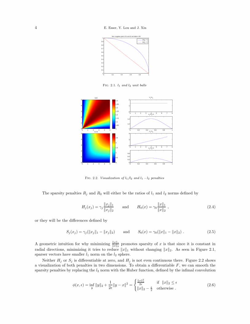
The sparsity penalties Rj and R0 will either be the ratios of l1 and l2 norms defined by
Hj(xj) = γj‖xj‖1‖xj‖2
and H0(x) = γ0‖x‖1‖x‖2
, (2.4)
or they will be the differences defined by
Sj(xj) = γj(‖xj‖1 − ‖xj‖2) and S0(x) = γ0(‖x‖1 − ‖x‖2) . (2.5)
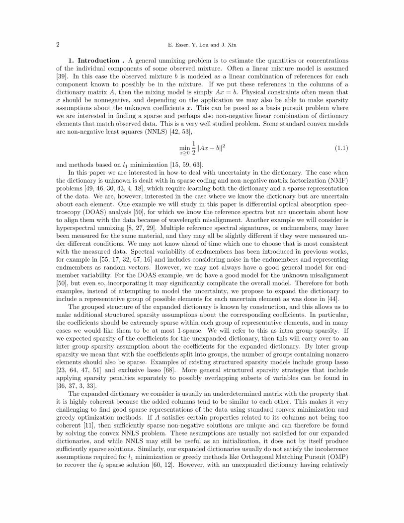
A geometric intuition for why minimizing ‖x‖1
‖x‖2
promotes sparsity of x is that since it is constant in
radial directions, minimizing it tries to reduce ‖x‖1 without changing ‖x‖2. As seen in Figure 2.1,sparser vectors have smaller l1 norm on the l2 sphere.
Neither Hj or Sj is differentiable at zero, and Hj is not even continuous there. Figure 2.2 showsa visualization of both penalties in two dimensions. To obtain a differentiable F , we can smooth thesparsity penalties by replacing the l2 norm with the Huber function, defined by the infimal convolution
φ(x, ǫ) = infy‖y‖2 +
1
2ǫ‖y − x‖2 =
{
‖x‖2
2
2ǫ if ‖x‖2 ≤ ǫ
‖x‖2 − ǫ2 otherwise .
(2.6)
A Method for Finding Structured Sparse Solutions 5
Regularized l1/l2
0 1 2 3 4 50
1
2
3
4
5
0.2
0.4
0.6
0.8
1
1.2
1.4
0 1 2 3 4 5 6 7 80
1
2
x1=x
2
0 0.2 0.4 0.6 0.8 11
1.2
1.4
x1+x
2=1
Regularized l1−l2
0 1 2 3 4 50
1
2
3
4
5
0
0.5
1
1.5
2
2.5
3
0 1 2 3 4 5 6 7 80
2
4
x1=x
2
0 0.2 0.4 0.6 0.8 10
0.2
0.4
0.6
x1+x
2=1
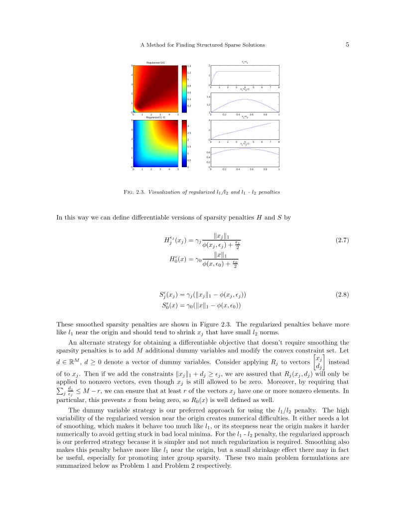
Fig. 2.3. Visualization of regularized l1/l2 and l1 - l2 penalties
In this way we can define differentiable versions of sparsity penalties H and S by
Hǫjj (xj) = γj
‖xj‖1φ(xj , ǫj) +
ǫj2
(2.7)
Hǫ0(x) = γ0
‖x‖1φ(x, ǫ0) +
ǫ02
Sǫj(xj) = γj(‖xj‖1 − φ(xj , ǫj)) (2.8)
Sǫ0(x) = γ0(‖x‖1 − φ(x, ǫ0))
These smoothed sparsity penalties are shown in Figure 2.3. The regularized penalties behave morelike l1 near the origin and should tend to shrink xj that have small l2 norms.
An alternate strategy for obtaining a differentiable objective that doesn’t require smoothing thesparsity penalties is to add M additional dummy variables and modify the convex constraint set. Let
d ∈ RM , d ≥ 0 denote a vector of dummy variables. Consider applying Rj to vectors
[
xj
dj
]
instead
of to xj . Then if we add the constraints ‖xj‖1 + dj ≥ ǫj , we are assured that Rj(xj , dj) will only beapplied to nonzero vectors, even though xj is still allowed to be zero. Moreover, by requiring that∑
jdj
ǫj≤ M − r, we can ensure that at least r of the vectors xj have one or more nonzero elements. In
particular, this prevents x from being zero, so R0(x) is well defined as well.
The dummy variable strategy is our preferred approach for using the l1/l2 penalty. The highvariability of the regularized version near the origin creates numerical difficulties. It either needs a lotof smoothing, which makes it behave too much like l1, or its steepness near the origin makes it hardernumerically to avoid getting stuck in bad local minima. For the l1 - l2 penalty, the regularized approachis our preferred strategy because it is simpler and not much regularization is required. Smoothing alsomakes this penalty behave more like l1 near the origin, but a small shrinkage effect there may in factbe useful, especially for promoting inter group sparsity. These two main problem formulations aresummarized below as Problem 1 and Problem 2 respectively.
6 E. Esser, Y. Lou and J. Xin
Problem 1:
minx,d
FH(x, d) :=1
2‖Ax− b‖2 +
M∑
j=1
γjHj(xj , dj) + γ0H0(x)
such that x > 0, d > 0,M∑
j=1
dj
ǫj≤ M − r and ‖xj‖1 + dj ≥ ǫj , j = 1, ...,M .
Problem 2:
minx≥0
FS(x) :=1
2‖Ax− b‖2 +
M∑
j=1
γjSǫj(xj) + γ0S
ǫ0(x) .
3. Algorithm . Both Problems 1 and 2 from Section 2 can be written abstractly as
minx∈X
F (x) :=1
2‖Ax− b‖2 +R(x), (3.1)
where X is a convex set. Problem 2 is already of this form with X = {x ∈ RN : x ≥ 0}. Problem
1 is also of this form, with X = {x ∈ RN , d ∈ R
M : x > 0, d > 0, ‖xj‖1 + dj ≥ ǫj ,∑
jdj
ǫj≤ M − r}.
Note that the objective function of Problem 1 can also be written as in (3.1) if we redefine xj as
[
xj
dj
]
and consider an expanded vector of coefficients x ∈ RN+M that includes the M dummy variables, d.
The data fidelity term can still be written as 12‖Ax − b‖2 if columns of zeros are inserted into A at
the indices corresponding to the dummy variables. In this section, we will describe algorithms andconvergence analysis for solving (3.1) under either of two sets of assumptions.
Assumption 1.
• X is a convex set.• R(x) ∈ C2(X,R) and the eigenvalues of ∇2R(x) are bounded on X.• F is coercive on X in the sense that for any x0 ∈ X, {x ∈ X : F (x) ≤ F (x0)} is a boundedset. In particular, F is bounded below.
Assumption 2.
• R(x) is concave and differentiable on X.• Same assumptions on X and F as in Assumption 1
Problem 1 satisfies Assumption 1 and Problem 2 satisfies Assumption 2. We will first consider thecase of Assumption 1.
Our approach for solving (3.1) was originally motivated by a convex splitting technique from[20, 61] that is a semi-implicit method for solving dx
dt= −∇F (x), x(0) = x0 when F can be split into
a sum of convex and concave functions FC(x) + FE(x), both in C2(RN ,R). Let λmaxFE be an upper
bound on the eigenvalues of ∇2FE , and let λminF be a lower bound on the eigenvalues of ∇2F . Under
the assumption that λmaxFE ≤ 1
2λminF it can be shown that the update defined by
xn+1 = xn −∆t(∇FC(xn+1) +∇FE(xn)) (3.2)
doesn’t increase F for any time step ∆t > 0. This can be seen by using second order Taylor expansionsto derive the estimate
F (xn+1)− F (xn) ≤ (λmaxFE − 1
2λminF − 1
∆t)‖xn+1 − xn‖2. (3.3)
This convex splitting approach has been shown to be an efficient method much faster than gradientdescent for solving phase-field models such as the Cahn-Hilliard equation, which has been used forexample to simulate coarsening [61] and for image inpainting [5].

A Method for Finding Structured Sparse Solutions 7
By the assumptions on R, we can achieve a convex concave splitting, F = FC + FE , by lettingFC(x) = 1
2‖Ax− b‖2 + ‖x‖2C and FE(x) = R(x)− ‖x‖2C for an appropriately chosen positive definitematrix C. We can also use the fact that FC(x) is quadratic to improve upon the estimate in (3.3)when bounding F (xn+1) − F (xn) by a quadratic function of xn+1. Then instead of choosing a timestep and updating according to (3.2), we can dispense with the time step interpretation altogether andchoose an update that reduces the upper bound on F (xn+1) − F (xn) as much as possible subject tothe constraint. This requires minimizing a strongly convex quadratic function over X .
Proposition 3.1. Let Assumption 1 hold. Also let λminR and λmax
R be lower and upper boundsrespectively on the eigenvalues of ∇2R(x) for x ∈ X. Then for x, y ∈ X and for any matrix C,
F (y)−F (x) ≤ (y−x)T ((λmaxR − 1
2λminR )I−C)(y−x)+(y−x)T (
1
2ATA+C)(y−x)+(y−x)T∇F (x) . (3.4)
Proof. The estimate follows from combining several second order Taylor expansions of F and R
with our assumptions. First expanding F about y and using h = y − x to simplify notation, we getthat
F (x) = F (y)− hT∇F (y) +1
2hT∇2F (y − α1h)h
for some α1 ∈ (0, 1). Substituting F as defined by (3.1), we obtain
F (y)− F (x) = hT (ATAy − AT b+∇R(y))− 1
2hTATAh− 1
2hT∇2R(y − α1h)h (3.5)
Similarly, we can compute Taylor expansions of R about both x and y.
R(x) = R(y)− hT∇R(y) +1
2hT∇2R(y − α2h)h .
R(y) = R(x) + hT∇R(x) +1
2hT∇2R(x+ α3h)h .
Again, both α2 and α3 are in (0, 1). Adding these expressions implies that
hT (∇R(y)−∇R(x)) =1
2hT∇2R(y − α2h)h+
1
2hT∇2R(x+ α3h)h .
From the assumption that the eigenvalues of ∇2R are bounded above by λmaxR on X ,
hT (∇R(y)−∇R(x)) ≤ λmaxR ‖h‖2 . (3.6)
Adding and subtracting hT∇R(x) and hTATAx to (3.5) yields
F (y)− F (x) = hTATAh+ hT (ATAx−AT b+∇R(x)) + hT (∇R(y)−∇R(x))
− 1
2hTATAh− 1
2hT∇2R(y − α1h)h
=1
2hTATAh+ hT∇F (x) + hT (∇R(y)−∇R(x)) − 1
2hT∇2R(y − α1h)h .
Using (3.6),
F (y)− F (x) ≤ 1
2hTATAh+ hT∇F (x)− 1
2hT∇2R(y − α1h)h+ λmax
R ‖h‖2 .
The assumption that the eigenvalues of ∇2R(x) are bounded below by λminR on X means
F (y)− F (x) ≤ (λmaxR − 1
2λminR )‖h‖2 + 1
2hTATAh+ hT∇F (x) .
8 E. Esser, Y. Lou and J. Xin
Since the estimate is unchanged by adding and subtracting hTCh for any matrix C, the inequality in(3.4) follows directly.
Corollary 3.2. Let C be symmetric positive definite and let λminC denote the smallest eigenvalue
of C. If λminC ≥ λmax
R − 12λ
minR , then for x, y ∈ X,
F (y)− F (x) ≤ (y − x)T (1
2ATA+ C)(y − x) + (y − x)T∇F (x) .
A natural strategy for solving (3.1) is then to iterate
xn+1 = argminx∈X
(x − xn)T (1
2ATA+ Cn)(x − xn) + (x− xn)T∇F (xn) (3.7)
for Cn chosen to guarantee a sufficient decrease in F . The method obtained by iterating (3.7) canbe viewed as an instance of scaled gradient projection [7, 6, 9] where the orthogonal projection ofxn−(ATA+2Cn)
−1∇F (xn) onto X is computed in the norm ‖·‖ATA+2Cn. The approach of decreasing
F by minimizing an upper bound coming from an estimate like (3.4) can be interpreted as majorization-minimization or an optimization transfer strategy of defining and minimizing a surrogate function [41],which is done for related applications in [30, 43]. It can also be interpreted as an example of theconcave-convex procedure (CCCP) [54, 65], a special case of difference of convex programming [57].
Choosing Cn in such a way that guarantees (xn+1 − xn)T ((λmaxR − 1
2λminR )I− Cn)(x
n+1 − xn) ≤ 0may be numerically inefficient, and it also isn’t strictly necessary for the algorithm to converge. Tosimplify the description of the algorithm, suppose Cn = cnC for some scalar cn > 0 and symmetricpositive definite C. Then as cn gets larger, the method becomes more like explicit gradient projectionwith small time steps. This can be slow to converge as well as more prone to converging to bad localminima. However, the method still converges as long as each cn is chosen so that the xn+1 updatedecreases F sufficiently. Therefore we want to dynamically choose cn ≥ 0 to be as small as possiblesuch that the xn+1 update given by (3.7) decreases F by a sufficient amount, namely
F (xn+1)− F (xn) ≤ σ
[
(xn+1 − xn)T (1
2ATA+ Cn)(x
n+1 − xn) + (xn+1 − xn)T∇F (xn)
]
for some σ ∈ (0, 1]. Additionally, we want to ensure that the modulus of strong convexity of thequadratic objective in (3.7) is large enough by requiring the smallest eigenvalue of 1
2ATA+ Cn to be
greater than or equal to some ρ > 0. The following is an algorithm for solving (3.1) and a dynamicupdate scheme for Cn = cnC that is similar to Armijo line search but designed to reduce the numberof times that the solution to the quadratic problem has to be rejected for not decreasing F sufficiently.
Algorithm 1: A Scaled Gradient Projection Method for Solving (3.1) Under Assumption 1
Define x0 ∈ X , c0 > 0, σ ∈ (0, 1], ǫ > 0, ρ > 0, ξ1 > 1, ξ2 > 1 and set n = 0.
while n = 0 or ‖xn − xn−1‖∞ > ǫ
y = argminx∈X
(x− xn)T (1
2ATA+ cnC)(x − xn) + (x − xn)T∇F (xn)
if F (y)− F (xn) > σ[
(y − xn)T (12ATA+ cnC)(y − xn) + (y − xn)T∇F (xn)
]
cn = ξ2cn
else
A Method for Finding Structured Sparse Solutions 9
xn+1 = y
cn+1 =
{
cnξ1
if smallest eigenvalue of cnξ1C + 1
2ATA is greater than ρ
cn otherwise .
n = n+ 1
end if
end while
It is not necessary to impose an upper bound on cn in Algorithm 1 even though we want it to bebounded. The reason for this is because once cn ≥ λmax
R − 12λ
minR , F will be sufficiently decreased for
any choice of σ ∈ (0, 1], so cn is effectively bounded by ξ2(λmaxR − 1
2λminR ).
Under Assumption 2 it is much more straightforward to derive an estimate analogous to Proposition3.1. Concavity of R(x) immediately implies
R(y) ≤ R(x) + (y − x)T∇R(x) .
Adding to this the expression
1
2‖Ay − b‖2 =
1
2‖Ax− b‖2 + (y − x)T (ATAx−AT b) +
1
2(y − x)TATA(y − x)
yields
F (y)− F (x) ≤ (y − x)T1
2ATA(y − x) + (y − x)T∇F (x) (3.8)
for x, y ∈ X . Moreover, the estimate still holds if we add (y − x)TC(y − x) to the right hand side forany positive semi-definite matrix C. We are again led to iterating (3.7) to decrease F , and in this caseCn need only be included to ensure that ATA + 2Cn is positive definite. We can let Cn = C sincethe dependence on n is no longer necessary. We can choose any C such that the smallest eigenvalueof C + 1
2ATA is greater than ρ > 0, but it is still preferable to choose C as small as is numerically
practical.
Algorithm 2: A Scaled Gradient Projection Method for Solving (3.1) Under Assumption 2
Define x0 ∈ X , C symmetric positive definite and ǫ > 0.
while n = 0 or ‖xn − xn−1‖∞ > ǫ
xn+1 = argminx∈X
(x− xn)T (1
2ATA+ C)(x − xn) + (x − xn)T∇F (xn) (3.9)
n = n+ 1
end while
Since the objective in (3.9) is zero at x = xn, the minimum value is less than or equal to zero, and soF (xn+1) ≤ F (xn) by (3.8).
Algorithm 2 is also equivalent to iterating
xn+1 = argminx∈X
1
2‖Ax− b‖2 + ‖x‖2C + xT (∇R(xn)− 2Cxn) ,
10 E. Esser, Y. Lou and J. Xin
which can be seen as an application of the simplified difference of convex algorithm from [57] toF (x) = (12‖Ax− b‖2 + ‖x‖2C)− (−R(x) + ‖x‖2C). The DC method in [57] is more general and doesn’trequire the convex and concave functions to be differentiable.
With many connections to classical algorithms, existing convergence results can be applied to arguethat limit points of the iterates {xn} of Algorithms 2 and 1 are stationary points of (3.1). We stillchoose to include a convergence analysis for clarity because our assumptions allow us to give a simpleand intuitive argument. The following analysis is for Algorithm 1 under Assumption 1. However, ifwe replace Cn with C and σ with 1, then it applies equally well to Algorithm 2 under Assumption 2.We proceed by showing that the sequence {xn} is bounded, ‖xn+1 − xn‖ → 0 and limit points of {xn}are stationary points of (3.1) satisfying the necessary local optimality condition (2.3).
Lemma 3.3. The sequence of iterates {xn} generated by Algorithm 1 is bounded.Proof. Since F (xn) is non-increasing, xn ∈ {x ∈ X : F (x) ≤ F (x0)}, which is a bounded set by
assumption.Lemma 3.4. Let {xn} be the sequence of iterates generated by Algorithm 1. Then ‖xn+1 − xn‖ →
0.Proof. Since {F (xn)} is bounded below and non-increasing, it converges. By construction, xn+1
satisfies
−[
(xn+1 − xn)T (1
2ATA+ Cn)(x
n+1 − xn) + (xn+1 − xn)T∇F (xn)
]
≤ 1
σ(F (xn)− F (xn+1)) .
By the optimality condition for (3.7),
(y − xn+1)T(
(ATA+ 2Cn)(xn+1 − xn) +∇F (xn)
)
≥ 0 ∀y ∈ X .
In particular, we can take y = xn, which implies
(xn+1 − xn)T (ATA+ 2Cn)(xn+1 − xn) ≤ −(xn+1 − xn)T∇F (xn) .
Thus
(xn+1 − xn)T (1
2ATA+ Cn)(x
n+1 − xn) ≤ 1
σ(F (xn)− F (xn+1)) .
Since the eigenvalues of 12A
TA+ Cn are bounded below by ρ > 0, we have that
ρ‖xn+1 − xn‖2 ≤ 1
σ(F (xn)− F (xn+1)) .
The result follows from noting that
limn→∞
‖xn+1 − xn‖2 ≤ limn→∞
1
σρ(F (xn)− F (xn+1)),
which equals 0 since {F (xn)} converges.Proposition 3.5. Any limit point x∗ of the sequence of iterates {xn} generated by Algorithm 1
satisfies (y − x∗)T∇F (x∗) ≥ 0 for all y ∈ X, which means x∗ is a stationary point of (3.1).Proof. Let x∗ be a limit point of {xn}. Since {xn} is bounded, such a point exists. Let {xnk} be
a subsequence that converges to x∗. Since ‖xn+1 − xn‖ → 0, we also have that xnk+1 → x∗. Recallingthe optimality condition for (3.7),
0 ≤ (y − xnk+1)T(
(ATA+ 2Cnk)(xnk+1 − xnk) +∇F (xnk)
)
≤‖y − xnk+1‖‖ATA+ 2Cnk
‖‖xnk+1 − xnk‖+ (y − xnk+1)T∇F (xnk) ∀y ∈ X .
Following [7], proceed by taking the limit along the subsequence as nk → ∞.
‖y − xnk+1‖‖xnk+1 − xnk‖‖ATA+ 2Cnk‖ → 0

A Method for Finding Structured Sparse Solutions 11
since ‖xnk+1 − xnk‖ → 0 and ‖ATA+ 2Cnk‖ is bounded. By continuity of ∇F we get that
(y − x∗)T∇F (x∗) ≥ 0 ∀y ∈ X .
Each iteration requires minimizing a strongly convex quadratic function over the set X as definedin (3.7). Many methods can be used to solve this, and we want to choose one that is as robust aspossible to poor conditioning of 1
2ATA+Cn. For example, gradient projection works theoretically and
even converges at a linear rate, but it can still be impractically slow. A better choice here is to use thealternating direction method of multipliers (ADMM) [24, 25], which alternately solves a linear systeminvolving 1
2ATA + Cn and projects onto the constraint set. Applied to Problem 2, this is essentially
the same as the application of split Bregman [26] to solve a NNLS model for hyperspectral unmixingin [56]. We consider separately the application of ADMM to Problems 1 and 2. The application toProblem 2 is simpler.
For Problem 2, (3.7) can be written as
xn+1 = argminx≥0
(x− xn)T (1
2ATA+ Cn)(x − xn) + (x− xn)T∇FS(x
n) .
To apply ADMM, we can first reformulate the problem as
minu,v
g≥0(v) + (u − xn)T (1
2ATA+ Cn)(u− xn) + (u − xn)T∇FS(x
n) such that u = v , (3.10)
where g is an indicator function for the constraint defined by g≥0(v) =
{
0 v ≥ 0
∞ otherwise.
Introduce a Lagrange multiplier p and define a Lagrangian
L(u, v, p) = g≥0(v) + (u− xn)T (1
2ATA+ Cn)(u − xn) + (u− xn)T∇FS(x
n) + pT (u− v) (3.11)
and augmented Lagrangian
Lδ(u, v, p) = L(u, v, p) +δ
2‖u− v‖2 ,
where δ > 0. ADMM finds a saddle point
L(u∗, v∗, p) ≤ L(u∗, v∗, p∗) ≤ L(u, v, p∗) ∀u, v, p
by alternately minimizing Lδ with respect to u, minimizing with respect to v and updating the dualvariable p. Having found a saddle point of L, (u∗, v∗) will be a solution to (3.10) and we can take v∗
to be the solution to (3.7). The explicit ADMM iterations are described in the following algorithm.
Algorithm 3: ADMM for solving convex subproblem for Problem 2
Define δ > 0, v0 and p0 arbitrarily and let k = 0.
while not converged
uk+1 = xn + (ATA+ 2Cn + δI)−1(
δ(vk − xn)− pk −∇FS(xn))
vk+1 = Π≥0
(
uk+1 +pk
δ
)
pk+1 = pk + δ(uk+1 − vk+1)

12 E. Esser, Y. Lou and J. Xin
k = k + 1
end while
Here Π≥0 denotes the orthogonal projection onto the non-negative orthant.
For Problem 2, (3.7) can be written as
(xn+1, dn+1) = argminx,d
(x− xn)T (1
2ATA+ Cx
n)(x− xn) + (d− dn)TCdn(d− dn)+
(x − xn)T∇xFH(xn, dn) + (d− dn)T∇dFH(xn, dn) .
Here, ∇x and ∇d represent the gradients with respect to x and d respectively. The matrix Cn is
assumed to be of the form Cn =
[
Cxn 00 Cd
n
]
, with Cdn a diagonal matrix. It is helpful to represent the
constraints in terms of convex sets defined by
Xǫj =
{[
xj
dj
]
∈ Rmj+1 : ‖xj‖1 + dj ≥ ǫj , xj ≥ 0, dj ≥ 0
}
j = 1, ...,M ,
Xβ =
d ∈ RM :
M∑
j=1
dj
βj
≤ M − r, dj ≥ 0
,
and indicator functions gXǫjand gXβ
for these sets.
Let u and w represent x and d. Then by adding splitting variables vx = u and vd = w we canreformulate the problem as
minu,w,vx,vd
∑
j
gXǫj(vxj , vdj) + gXβ
(w) + (u− xn)T (1
2ATA+ Cx
n)(u− xn) + (w − dn)TCdn(w − dn)+
(x− xn)T∇xFH(xn, dn) + (w − dn)T∇dFH(xn, dn) s.t. vx = u, vd = w .
Adding Lagrange multipliers px and pd for the linear constraints, we can define the augmented La-grangian
Lδ(u,w, vx, vd, px, pd) =∑
j
gXǫj(vxj , vdj) + gXβ
(w) + (u − xn)T (1
2ATA+ Cx
n)(u− xn)+
(w − dn)TCdn(w − dn) + (x− xn)T∇xFH(xn, dn) + (w − dn)T∇dFH(xn, dn)+
pTx (u− vx) + pTd (w − vd) +δ
2‖u− vx‖2 +
δ
2‖w − vd‖2 .
Each ADMM iteration alternately minimizes Lδ first with respect to (u,w) and then with respectto (vx, vd) before updating the dual variables (px, pd). The explicit iterations are described in thefollowing algorithm.
A Method for Finding Structured Sparse Solutions 13
Algorithm 4: ADMM for solving convex subproblem for Problem 1
Define δ > 0, v0x, v0d, p
0x and p0d arbitrarily and let k = 0.
Define the weights β in the projection ΠXβby βj = (ǫj
√
(2Cdn + δI)j,j)
−1 j = 1, ...,M .
while not converged
uk+1 = xn + (ATA+ 2Cxn + δI)−1
(
δ(vkx − xn)− pkx −∇xFH(xn, dn))
wk+1 = (2Cdn + δI)−
1
2ΠXβ
(
(2Cdn + δI)−
1
2 (δvkd − pkd −∇dFH(xn, dn) + 2Cdn))
[
vxjvdj
]k+1
= ΠXǫj
uk+1j +
pxkj
δ
wk+1j +
pkdj
δ
j = 1, ...,M
pk+1x = pkx + δ(uk+1 − vk+1
x )
pk+1d = pkd + δ(wk+1 − vk+1
d )
k = k + 1
end while
We stop iterating and let xn+1 = vx and dn+1 = vd once the relative errors of the primal anddual variables are sufficiently small. The projections ΠXβ
and ΠXǫjcan be efficiently computed by
combining projections onto the non-negative orthant and projections onto the appropriate simplices.These can in principle be computed in linear time [10], although we use a method that is simpler toimplement and is still only O(n log n) in the dimension of the vector being projected.
Since (3.7) is a standard quadratic program, a huge variety of other methods besides ADMM couldalso be applied. Variants of Newton’s method on a bound constrained Karush-Kuhn-Tucker (KKT)system might work well if we find we need to solve the convex subproblems to very high accuracy. Forthe above applications of ADMM to be practical, the linear system involving (ATA+2Cn+ δI) shouldnot be too difficult to solve, and δ should be well chosen. It may sometimes be helpful to use theWoodbury formula, c(ATA+ cI)−1 = I−AT (cI+AAT )−1A, which means we can choose to work withATA or AAT , whichever is smaller. Additionally, the linear systems could be approximately solved byiterative methods such as preconditioned conjugate gradient. It may also be worthwhile to considerprimal dual methods that only require matrix multiplications [14, 19]. The simplest alternative mightbe to apply gradient projection directly to (3.1). This can be thought of as applying the DC methodto a different convex-concave splitting of F , namely F (x) = (‖x‖2C)− (‖x‖2C − 1
2‖Ax− b‖2 −R(x)) forsufficiently large C [58], but gradient projection may be too inefficient when A is ill-conditioned.
4. Applications . In this section we introduce four specific applications related to DOAS analysisand hyperspectral unmixing. We show how to model these problems in the form of (3.1) so that thealgorithms from Section 3 can be applied.
4.1. DOAS Analysis. The goal of DOAS is to estimate the concentrations of gases in a mixtureby measuring over a range of wavelengths the reduction in the intensity of light shined through it. Athorough summary of the procedure and analysis can be found in [50].
Beer’s law can be used to estimate the attenuation of light intensity due to absorption. Assumingthe average gas concentration c is not too large, Beer’s law relates the transmitted intensity I(λ) tothe initial intensity I0(λ) by
I(λ) = I0(λ) exp−σ(λ)cL, (4.1)
14 E. Esser, Y. Lou and J. Xin
where λ is wavelength, σ(λ) is the characteristic absorption spectra for the absorbing gas and L is thelight path length.
If the density of the absorbing gas is not constant, we should instead integrate over the light
path, replacing exp−σ(λ)cL by exp−σ(λ)∫
L
0c(l)dl. For simplicity, we will assume the concentration is
approximately constant. We will also denote the product of concentration and path length, cL, by a.When multiple absorbing gases are present, aσ(λ) can be replaced by a linear combination of the
characteristic absorption spectra of the gases, and Beer’s law can be written as
I(λ) = I0(λ) exp−∑
jajσj(λ) .
Additionally taking into account the reduction of light intensity due to scattering, combined intoa single term ǫ(λ), Beer’s law becomes
I(λ) = I0(λ) exp−∑
jajσj(λ)−ǫ(λ) .
The key idea behind DOAS is that it is not necessary to explicitly model effects such as scattering,as long as they vary smoothly enough with wavelength to be removed by high pass filtering that looselyspeaking removes the broad structures and keeps the narrow structures. We will assume that ǫ(λ) issmooth. Additionally, we can assume that I0(λ), if not known, is also smooth. The absorption spectraσj(λ) can be considered to be a sum of a broad part (smooth) and a narrow part, σj = σbroad
j +σnarrowj . Since σnarrow
j represents the only narrow structure in the entire model, the main idea is toisolate it by taking the log of the intensity and applying high pass filtering or any other procedure, suchas polynomial fitting, that subtracts a smooth background from the data. The given reference spectrashould already have had their broad parts subtracted, but it may not have been done consistently,so we will combine σbroad
j and ǫ(λ) into a single term B(λ). We will also denote the given referencespectra by yj , which again are already assumed to be approximately high pass filtered versions of thetrue absorption spectra σj . With these notational changes, Beer’s law becomes
I(λ) = I0(λ) exp−
∑j ajyj(λ)−B(λ) . (4.2)
In practice, measurement errors must also be modeled. We therefore consider multiplying the righthand side of (4.2) by s(λ), representing wavelength dependent sensitivity. Assuming that s(λ) ≈ 1and varies smoothly with λ, we can absorb it into B(λ). Measurements may also be corrupted byconvolution with an instrument function h(λ), but for simplicity we will assume this effect is negligibleand not include convolution with h in the model. Let J(λ) = − ln(I(λ)). This is what we will considerto be the given data. By taking the log, the previous model simplifies to
J(λ) = − ln(I0(λ)) +∑
j
ajyj(λ) + B(λ) + η(λ),
where η(λ) represents the log of multiplicative noise, which we will model as being approximatelywhite Gaussian noise.
Since I0(λ) is assumed to be smooth, it can also be absorbed into the B(λ) component, yieldingthe data model
J(λ) =∑
j
ajyj(λ) +B(λ) + η(λ). (4.3)
4.1.1. DOAS Analysis with Wavelength Misalignment . A challenging complication inpractice is wavelength misalignment, i.e., the nominal wavelengths in the measurement J(λ) may notcorrespond exactly to those in the basis yj(λ). We must allow for small, often approximately lineardeformations vj(λ) so that yj(λ + vj(λ)) are all aligned with the data J(λ). Taking into accountwavelength misalignment, the data model becomes
J(λ) =∑
j
ajyj(λ+ vj(λ)) +B(λ) + η(λ). (4.4)

A Method for Finding Structured Sparse Solutions 15
To first focus on the alignment aspect of this problem, assume B(λ) is negligible, having somehowbeen consistently removed from the data and references by high pass filtering or polynomial subtraction.Then given the data J(λ) and reference spectra {yj(λ)}, we want to estimate the fitting coefficients{aj} and the deformations {vj(λ)} from the linear model,
J(λ) =
M∑
j=1
ajyj(
λ+ vj(λ))
+ η(λ) , (4.5)
where M is the total number of gases to be considered.Inspired by the idea of using a set of modified bases for image deconvolution [44], we construct a
dictionary by deforming each yj with a set of possible deformations. Specifically, since the deformationscan be well approximated by linear functions, i.e., vj(λ) = pjλ + qj , we enumerate all the possibledeformations by choosing pj , qj from two pre-determined sets {P1, · · · , PK}, {Q1, · · · , QL}. Let Aj
be a matrix whose columns are deformations of the jth reference yj(λ), i.e., yj(λ + Pkλ + Ql) fork = 1, · · · ,K and l = 1, · · · , L. Then we can rewrite the model (4.5) in terms of a matrix-vector form,
J = [A1, · · · , AM ]
x1
...xM
+ η , (4.6)
where xj ∈ RKL and J ∈ R
W .We propose the following minimization model,
argminxj
12‖J − [A1, · · · , AM ]
x1
...xM
‖2 ,
s.t. xj > 0, ‖xj‖0 6 1 j = 1, · · · ,M .
(4.7)
The second constraint in (4.7) is to enforce each xj to have at most one non-zero element. Having‖xj‖0 = 1 indicates the existence of the gas with a spectrum yj Its non-zero index corresponds to theselected deformation and its magnitude corresponds to the concentration of the gas. This l0 constraintmakes the problem NP-hard. A direct approach is the penalty decomposition method proposed in [45],which we will compare to in Section 5. Our approach is to replace the l0 constraint on each groupwith intra sparsity penalties defined by Hj in (2.4) or Sǫ
j in (2.8), putting the problem in the form ofProblem 1 or Problem 2. The intra sparsity parameters γj should be chosen large enough to enforce1-sparsity within groups, and in the absence of any inter group sparsity assumptions we can set γ0 = 0.
4.1.2. DOAS with Background Model. To incorporate the background term from (4.4), wewill add B ∈ R
W as an additional unknown and also add a quadratic penalty α2 ‖QB‖2 to penalize a
lack of smoothness of B. This leads to the model
minx∈X,B
1
2‖Ax+B − J‖2 + α
2‖QB‖2 +R(x) ,
where R includes our choice of intra sparsity penalties on x. This can be rewritten as
minx∈X,B
1
2
∥
∥
∥
∥
[
A I0
√αQ
] [
x
B
]
−[
J
0
]∥
∥
∥
∥
2
+ R(x) . (4.8)
This has the general form of (3.1) with the two by two block matrix interpreted asA and
[
J
0
]
interpreted
as b. Moreover, we can concatenate B and the M groups xj by considering B to be group xM+1 andsetting γM+1 = 0 so that no sparsity penalty acts on the background component. In this way, we seethat the algorithms presented in Section 3 can be directly applied to (4.8).
16 E. Esser, Y. Lou and J. Xin
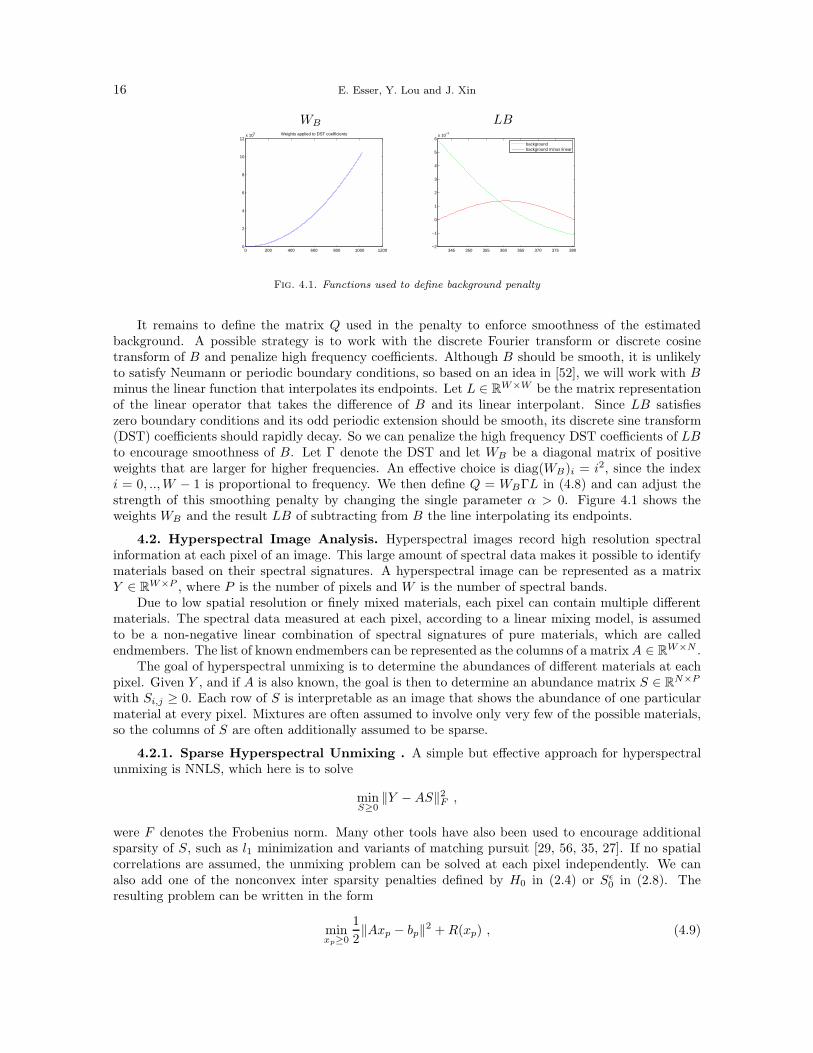
WB LB
0 200 400 600 800 1000 12000
2
4
6
8
10
12x 10
5 Weights applied to DST coefficients
345 350 355 360 365 370 375 380−2
−1
0
1
2
3
4
5
6x 10
−3
backgroundbackground minus linear
Fig. 4.1. Functions used to define background penalty
It remains to define the matrix Q used in the penalty to enforce smoothness of the estimatedbackground. A possible strategy is to work with the discrete Fourier transform or discrete cosinetransform of B and penalize high frequency coefficients. Although B should be smooth, it is unlikelyto satisfy Neumann or periodic boundary conditions, so based on an idea in [52], we will work with B
minus the linear function that interpolates its endpoints. Let L ∈ RW×W be the matrix representation
of the linear operator that takes the difference of B and its linear interpolant. Since LB satisfieszero boundary conditions and its odd periodic extension should be smooth, its discrete sine transform(DST) coefficients should rapidly decay. So we can penalize the high frequency DST coefficients of LBto encourage smoothness of B. Let Γ denote the DST and let WB be a diagonal matrix of positiveweights that are larger for higher frequencies. An effective choice is diag(WB)i = i2, since the indexi = 0, ..,W − 1 is proportional to frequency. We then define Q = WBΓL in (4.8) and can adjust thestrength of this smoothing penalty by changing the single parameter α > 0. Figure 4.1 shows theweights WB and the result LB of subtracting from B the line interpolating its endpoints.
4.2. Hyperspectral Image Analysis. Hyperspectral images record high resolution spectralinformation at each pixel of an image. This large amount of spectral data makes it possible to identifymaterials based on their spectral signatures. A hyperspectral image can be represented as a matrixY ∈ R
W×P , where P is the number of pixels and W is the number of spectral bands.Due to low spatial resolution or finely mixed materials, each pixel can contain multiple different
materials. The spectral data measured at each pixel, according to a linear mixing model, is assumedto be a non-negative linear combination of spectral signatures of pure materials, which are calledendmembers. The list of known endmembers can be represented as the columns of a matrixA ∈ R
W×N .The goal of hyperspectral unmixing is to determine the abundances of different materials at each
pixel. Given Y , and if A is also known, the goal is then to determine an abundance matrix S ∈ RN×P
with Si,j ≥ 0. Each row of S is interpretable as an image that shows the abundance of one particularmaterial at every pixel. Mixtures are often assumed to involve only very few of the possible materials,so the columns of S are often additionally assumed to be sparse.
4.2.1. Sparse Hyperspectral Unmixing . A simple but effective approach for hyperspectralunmixing is NNLS, which here is to solve
minS≥0
‖Y −AS‖2F ,
were F denotes the Frobenius norm. Many other tools have also been used to encourage additionalsparsity of S, such as l1 minimization and variants of matching pursuit [29, 56, 35, 27]. If no spatialcorrelations are assumed, the unmixing problem can be solved at each pixel independently. We canalso add one of the nonconvex inter sparsity penalties defined by H0 in (2.4) or Sǫ
0 in (2.8). Theresulting problem can be written in the form
minxp≥0
1
2‖Axp − bp‖2 +R(xp) , (4.9)
A Method for Finding Structured Sparse Solutions 17
where xp is the pth column of S and bp is the pth column of Y . We can define R(xp) to equal H0(xp)or Sǫ
0(xp), putting (4.9) in the general form of (3.1).
4.2.2. Structured Sparse Hyperspectral Unmixing. In hyperspectral unmixing applica-tions, the dictionary of endmembers is usually not known precisely. There are many methods forlearning endmembers from a hyperspectral image such as N-FINDR [62], vertex component analysis(VCA) [48], NMF [49], Bayesian methods [66, 13] and convex optimization [18]. However, here weare interested in the case where we have a large library of measured reference endmembers includingmultiple references for each expected material measured under different conditions. The resulting dic-tionary A is assumed to have the group structure [A1, · · · , AM ], where each group Aj contains differentreferences for the same jth material.
There are several reasons that we don’t want to use the sparse unmixing methods of Section 4.2.1when A contains a large library of references defined in this way. Such a matrix A with many nearlyredundant references will likely have high coherence. This creates a challenge for existing methods.The grouped structure of A also means that we want to enforce a structured sparsity assumption on thecolumns of S. The linear combination of endmembers at any particular pixel is assumed to involve atmost one endmember from each group Aj . Linearly combining multiple references within a group maynot be physically meaningful, since they all represent the same material. Restricting our attention to
a single pixel p, we can write the pth abundance column xp of S as
x1,p
...xM,p
. The sparsity assumption
requires each group of abundance coefficients xj,p to be at most one sparse. We can enforce this byadding sufficiently large intra sparsity penalties to the objective in (4.9) defined by Hj(xj,p) (2.4) orSǫj(xj,p) (2.8).
We think it may be important to use an expanded dictionary to allow different endmembers withingroups to be selected at different pixels, thus incorporating endmember variability into the unmixingprocess. Existing methods accomplish this in different ways, such as the piece-wise convex endmemberdetection method in [67], which represents the spectral data as convex combinations of endmemberdistributions. It is observed in [67] that real hyperspectral data can be better represented using severalsets of endmembers. Additionally, their better performance compared to VCA, which assumes pixelpurity, on a dataset which should satisfy the pixel purity assumption, further justifies the benefit ofincorporating endmember variability when unmixing.
If the same set of endmembers were valid at all pixels, we could attempt to enforce row sparsity ofS using for example the l1,∞ penalty used in [18], which would encourage the data at all pixels to berepresentable as non-negative linear combinations of the same small subset of endmembers. Under somecircumstances, this is a reasonable assumption and could be a good approach. However, due to varyingconditions, a particular reference for some material may be good at some pixels but not at others.Although atmospheric conditions are of course unlikely to change from pixel to pixel, there could benonlinear mixing effects that make the same material appear to have different spectral signatures indifferent locations [39]. For instance, a nonuniform layer of dust will change the appearance of materialsin different places. If this mixing with dust is nonlinear, then the resulting hyperspectral data cannotnecessarily be well represented by the linear mixture model with a dust endmember added to thedictionary. In this case, by considering an expanded dictionary containing reference measurementsfor the materials covered by different amounts of dust, we are attempting to take into account thesenonlinear mixing effects without explicitly modeling them. At different pixels, different references forthe same materials can now be used when trying to best represent the data. We should point out thatour approach is effective when only a small number of nonlinear effects need to be taken into account.The more spectral variability we include for each endmember, the larger the matrix A becomes. Ourmethod is applicable when there are relatively few realizations of endmember variability in the dataand these realizations are well represented in the expanded dictionary.
The overall model should contain both intra and inter sparsity penalties. In addition to the onesparsity assumption within groups, it is still assumed that many fewer than M materials are present
18 E. Esser, Y. Lou and J. Xin
at any particular pixel. The full model can again be written as (4.9) except with the addition of intrasparsity penalties. The overall sparsity penalties can be written either as
R(xp, dp) =
M∑
j=1
γjHj(xj,p, dj,p) + γ0H0(xp)
or
R(xp) =
M∑
j=1
γjSǫjj (xj,p) + γ0S
ǫ00 (xp) .
5. Numerical Experiments . In this section, we evaluate the effectiveness of our implementa-tions of Problems 1 and 2 on the four applications discussed in Section 4. The simplest DOAS examplewith wavelength misalignment from Section 4.1.1 is used to see how well the intra sparsity assumptionis satisfied compared to other methods. Two convex methods that we compare to are NNLS (1.1) anda non-negative constrained l1 basis pursuit model like the template matching via l1 minimization in[28]. The l1 minimization model we use here is
minx≥0
‖x‖1 such that ‖Ax− b‖ ≤ τ . (5.1)
We use MATLAB’s lsqnonneg function, which is parameter free, to solve the NNLS model. We useBregman iteration [63] to solve the l1 minimization model. We also compare to direct l0 minimizationvia penalty decomposition (Algorithm 5).
The penalty decomposition method [45] amounts to solving (4.7) by a series of minimizationproblems with an increasing sequence {ρk}. Let x = [x1, · · · ,xM ], y = [y1, · · · ,yM ] and iterate
(xk+1, yk+1) = argmin 12‖Ax− b‖2 + ρk
2 ‖x− y‖2s.t. yj > 0, ‖yj‖0 6 1
ρk+1 = σρk (for σ > 1) .(5.2)
The pseudo-code of this method is given in Algorithm 5.
Algorithm 5: A penalty decomposition method for solving (4.7)
Define ρ > 0, σ > 1, ǫo, ǫi and initialize y.
while ‖x− y‖∞ > ǫoi = 1;while max{‖xi − xi−1‖∞, ‖yi − yi−1‖∞} > ǫi
xi = (ATA+ ρId)−1(AT b+ ρyi)yi = 0for j = 1, · · · ,M
find the index of maximal xj , i.e., lj = argmaxl xj(l)Set yj(lj) = max(xj(lj), 0)
end for
i = i+1;end while
x = xi, y = yi, ρ = σρ
end while
A Method for Finding Structured Sparse Solutions 19
HONO NO2 O3
340 345 350 355 360 365 370 375 380 385−0.04
−0.02
0
0.02
0.04
0.06
0.08
0.1
0.12
0.14
340 345 350 355 360 365 370 375 380 385−0.1
−0.08
−0.06
−0.04
−0.02
0
0.02
0.04
0.06
0.08
0.1
340 345 350 355 360 365 370 375 380 3850
0.02
0.04
0.06
0.08
0.1
0.12
0.14
0.16
Fig. 5.1. For each gas, the reference spectrum is plotted in red, while three deformed spectra are in blue.
Algorithm 5 may require a good initialization of y or a slowly increasing ρ. If the maximummagnitude locations within each group are initially incorrect, it can get stuck at a local minimum.We consider both least square (LS) and NNLS initializations in numerical experiments. Algorithms 1and 2 also benefit from a good initialization for the same reason. We use a constant initialization, forwhich the first iteration of those methods is already quite similar to NNLS.
We also test the effectiveness of Problems 1 and 2 on the three other applications discussed inSection 4. For DOAS with the included background model, we compare again to Algorithm 5. We usethe sparse hyperspectral unmixing example to demonstrate the sparsifying effect of the inter sparsitypenalties acting without any intra sparsity penalties. We compare to the l1 regularized unmixingmodel in [29] using the implementation in [56]. To illustrate the effect of the intra and inter sparsitypenalties acting together, we also apply Problems 1 and 2 to a synthetic example of structured sparsehyperspectral unmixing. We compare the recovery of the ground truth abundance with and withoutthe intra sparsity penalties.
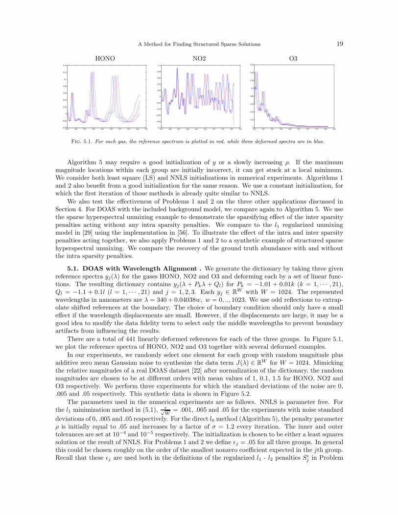
5.1. DOAS with Wavelength Alignment . We generate the dictionary by taking three givenreference spectra yj(λ) for the gases HONO, NO2 and O3 and deforming each by a set of linear func-tions. The resulting dictionary contains yj(λ + Pkλ + Ql) for Pk = −1.01 + 0.01k (k = 1, · · · , 21),Ql = −1.1 + 0.1l (l = 1, · · · , 21) and j = 1, 2, 3. Each yj ∈ R
W with W = 1024. The representedwavelengths in nanometers are λ = 340 + 0.04038w, w = 0, .., 1023. We use odd reflections to extrap-olate shifted references at the boundary. The choice of boundary condition should only have a smalleffect if the wavelength displacements are small. However, if the displacements are large, it may be agood idea to modify the data fidelity term to select only the middle wavelengths to prevent boundaryartifacts from influencing the results.
There are a total of 441 linearly deformed references for each of the three groups. In Figure 5.1,we plot the reference spectra of HONO, NO2 and O3 together with several deformed examples.
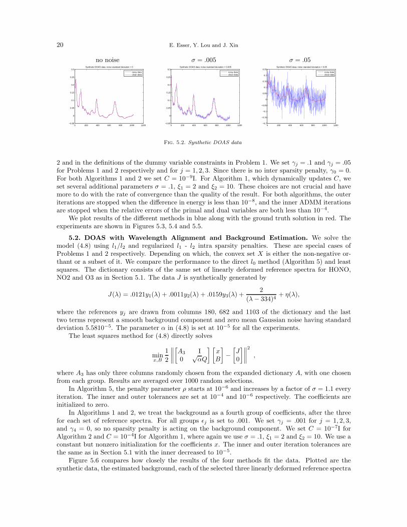
In our experiments, we randomly select one element for each group with random magnitude plusadditive zero mean Gaussian noise to synthesize the data term J(λ) ∈ R
W for W = 1024. Mimickingthe relative magnitudes of a real DOAS dataset [22] after normalization of the dictionary, the randommagnitudes are chosen to be at different orders with mean values of 1, 0.1, 1.5 for HONO, NO2 andO3 respectively. We perform three experiments for which the standard deviations of the noise are 0,.005 and .05 respectively. This synthetic data is shown in Figure 5.2.
The parameters used in the numerical experiments are as follows. NNLS is parameter free. Forthe l1 minimization method in (5.1), τ√
W= .001, .005 and .05 for the experiments with noise standard
deviations of 0, .005 and .05 respectively. For the direct l0 method (Algorithm 5), the penalty parameterρ is initially equal to .05 and increases by a factor of σ = 1.2 every iteration. The inner and outertolerances are set at 10−4 and 10−5 respectively. The initialization is chosen to be either a least squaressolution or the result of NNLS. For Problems 1 and 2 we define ǫj = .05 for all three groups. In generalthis could be chosen roughly on the order of the smallest nonzero coefficient expected in the jth group.Recall that these ǫj are used both in the definitions of the regularized l1 - l2 penalties Sǫ
j in Problem
20 E. Esser, Y. Lou and J. Xin
no noise σ = .005 σ = .05
0 200 400 600 800 1000 1200−0.05
0
0.05
0.1
0.15
0.2
0.25
0.3Synthetic DOAS data: noise standard deviation = 0
noisy dataclean data
0 200 400 600 800 1000 1200−0.05
0
0.05
0.1
0.15
0.2
0.25
0.3Synthetic DOAS data: noise standard deviation = 0.005
noisy dataclean data
0 200 400 600 800 1000 1200−0.2
−0.15
−0.1
−0.05
0
0.05
0.1
0.15
0.2
0.25Synthetic DOAS data: noise standard deviation = 0.05
noisy dataclean data
Fig. 5.2. Synthetic DOAS data
2 and in the definitions of the dummy variable constraints in Problem 1. We set γj = .1 and γj = .05for Problems 1 and 2 respectively and for j = 1, 2, 3. Since there is no inter sparsity penalty, γ0 = 0.For both Algorithms 1 and 2 we set C = 10−9I. For Algorithm 1, which dynamically updates C, weset several additional parameters σ = .1, ξ1 = 2 and ξ2 = 10. These choices are not crucial and havemore to do with the rate of convergence than the quality of the result. For both algorithms, the outeriterations are stopped when the difference in energy is less than 10−8, and the inner ADMM iterationsare stopped when the relative errors of the primal and dual variables are both less than 10−4.
We plot results of the different methods in blue along with the ground truth solution in red. Theexperiments are shown in Figures 5.3, 5.4 and 5.5.
5.2. DOAS with Wavelength Alignment and Background Estimation. We solve themodel (4.8) using l1/l2 and regularized l1 - l2 intra sparsity penalties. These are special cases ofProblems 1 and 2 respectively. Depending on which, the convex set X is either the non-negative or-thant or a subset of it. We compare the performance to the direct l0 method (Algorithm 5) and leastsquares. The dictionary consists of the same set of linearly deformed reference spectra for HONO,NO2 and O3 as in Section 5.1. The data J is synthetically generated by
J(λ) = .0121y1(λ) + .0011y2(λ) + .0159y3(λ) +2
(λ− 334)4+ η(λ),
where the references yj are drawn from columns 180, 682 and 1103 of the dictionary and the lasttwo terms represent a smooth background component and zero mean Gaussian noise having standarddeviation 5.5810−5. The parameter α in (4.8) is set at 10−5 for all the experiments.
The least squares method for (4.8) directly solves
minx,B
1
2
∥
∥
∥
∥
[
A3 I0
√αQ
] [
x
B
]
−[
J
0
]∥
∥
∥
∥
2
,
where A3 has only three columns randomly chosen from the expanded dictionary A, with one chosenfrom each group. Results are averaged over 1000 random selections.
In Algorithm 5, the penalty parameter ρ starts at 10−6 and increases by a factor of σ = 1.1 everyiteration. The inner and outer tolerances are set at 10−4 and 10−6 respectively. The coefficients areinitialized to zero.
In Algorithms 1 and 2, we treat the background as a fourth group of coefficients, after the threefor each set of reference spectra. For all groups ǫj is set to .001. We set γj = .001 for j = 1, 2, 3,and γ4 = 0, so no sparsity penalty is acting on the background component. We set C = 10−7I forAlgorithm 2 and C = 10−4I for Algorithm 1, where again we use σ = .1, ξ1 = 2 and ξ2 = 10. We use aconstant but nonzero initialization for the coefficients x. The inner and outer iteration tolerances arethe same as in Section 5.1 with the inner decreased to 10−5.
Figure 5.6 compares how closely the results of the four methods fit the data. Plotted are thesynthetic data, the estimated background, each of the selected three linearly deformed reference spectra
A Method for Finding Structured Sparse Solutions 21
200 400 600 800 1000 12000
1
2NNLS
200 400 600 800 1000 12000
1
2l1
200 400 600 800 1000 12000
1
2Least squares + l0
200 400 600 800 1000 12000
1
2NNLS + l0
200 400 600 800 1000 12000
1
2l1/l2
200 400 600 800 1000 12000
1
2l1−l2 (regularized)
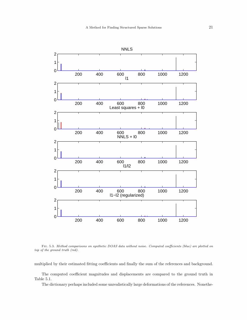
Fig. 5.3. Method comparisons on synthetic DOAS data without noise. Computed coefficients (blue) are plotted ontop of the ground truth (red).
multiplied by their estimated fitting coefficients and finally the sum of the references and background.
The computed coefficient magnitudes and displacements are compared to the ground truth inTable 5.1.
The dictionary perhaps included some unrealistically large deformations of the references. Nonethe-
22 E. Esser, Y. Lou and J. Xin
200 400 600 800 1000 12000
1
2NNLS
200 400 600 800 1000 12000
1
2l1
200 400 600 800 1000 12000
1
2Least squares + l0
200 400 600 800 1000 12000
1
2NNLS + l0
200 400 600 800 1000 12000
1
2l1/l2
200 400 600 800 1000 12000
1
2l1−l2 (regularized)
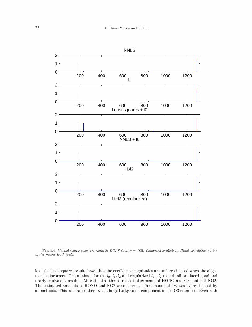
Fig. 5.4. Method comparisons on synthetic DOAS data: σ = .005. Computed coefficients (blue) are plotted on topof the ground truth (red).
less, the least squares result shows that the coefficient magnitudes are underestimated when the align-ment is incorrect. The methods for the l0, l1/l2 and regularized l1 - l2 models all produced good andnearly equivalent results. All estimated the correct displacements of HONO and O3, but not NO2.The estimated amounts of HONO and NO2 were correct. The amount of O3 was overestimated byall methods. This is because there was a large background component in the O3 reference. Even with
A Method for Finding Structured Sparse Solutions 23
200 400 600 800 1000 12000
1
2NNLS
200 400 600 800 1000 12000
1
2l1
200 400 600 800 1000 12000
1
2Least squares + l0
200 400 600 800 1000 12000
1
2NNLS + l0
200 400 600 800 1000 12000
1
2l1/l2
200 400 600 800 1000 12000
1
2l1−l2 (regularized)
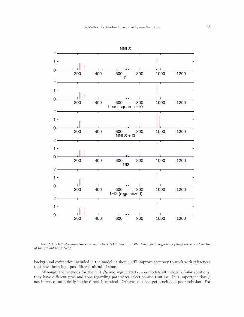
Fig. 5.5. Method comparisons on synthetic DOAS data: σ = .05. Computed coefficients (blue) are plotted on topof the ground truth (red).
background estimation included in the model, it should still improve accuracy to work with referencesthat have been high pass filtered ahead of time.
Although the methods for the l0, l1/l2 and regularized l1 - l2 models all yielded similar solutions,they have different pros and cons regarding parameter selection and runtime. It is important that ρ
not increase too quickly in the direct l0 method. Otherwise it can get stuck at a poor solution. For
24 E. Esser, Y. Lou and J. Xin
340 350 360 370 380 390−1
0
1
2
3
4x 10
−3
wavelength
Average of random least squares fits
databackgroundHONONO2O3fit
340 350 360 370 380 390−1
0
1
2
3
4x 10
−3
wavelength
l0 fit
databackgroundHONONO2O3fit
340 350 360 370 380 390−1
0
1
2
3
4x 10
−3
wavelength
l1/l2 fit
databackgroundHONONO2O3fit
340 350 360 370 380 390−1
0
1
2
3
4x 10
−3
wavelength
l1 − l2 fit
databackgroundHONONO2O3fit
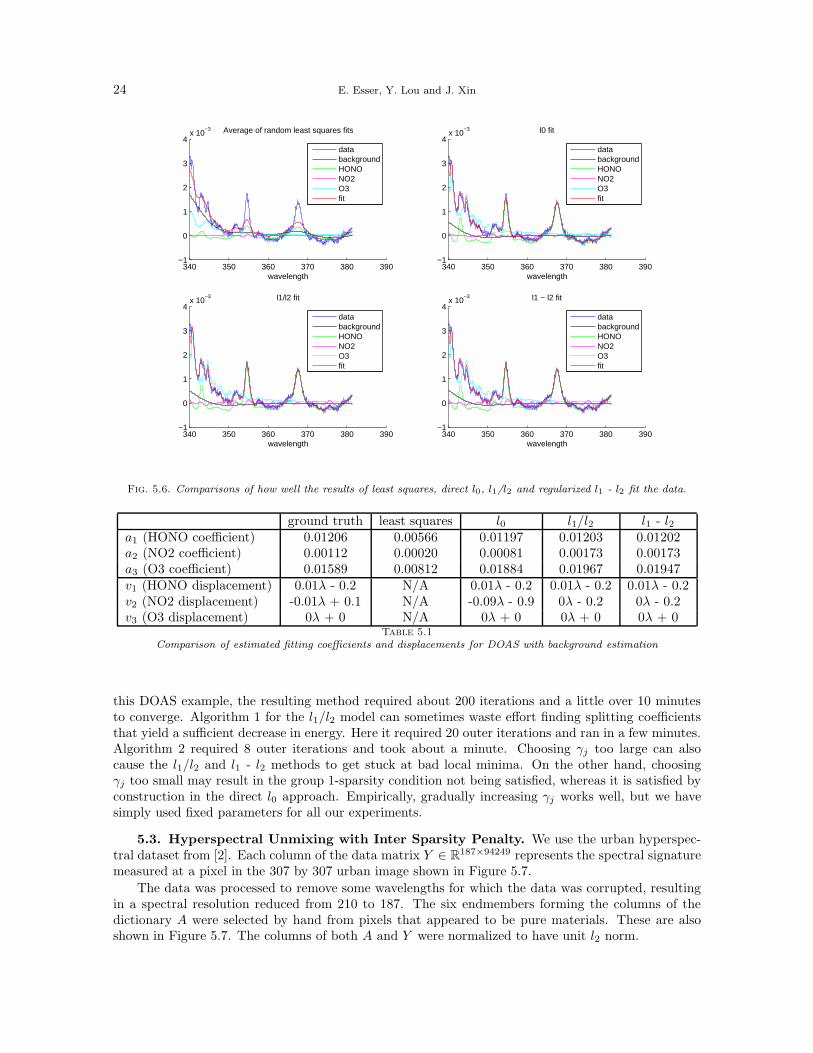
Fig. 5.6. Comparisons of how well the results of least squares, direct l0, l1/l2 and regularized l1 - l2 fit the data.
ground truth least squares l0 l1/l2 l1 - l2a1 (HONO coefficient) 0.01206 0.00566 0.01197 0.01203 0.01202a2 (NO2 coefficient) 0.00112 0.00020 0.00081 0.00173 0.00173a3 (O3 coefficient) 0.01589 0.00812 0.01884 0.01967 0.01947v1 (HONO displacement) 0.01λ - 0.2 N/A 0.01λ - 0.2 0.01λ - 0.2 0.01λ - 0.2v2 (NO2 displacement) -0.01λ + 0.1 N/A -0.09λ - 0.9 0λ - 0.2 0λ - 0.2v3 (O3 displacement) 0λ + 0 N/A 0λ + 0 0λ + 0 0λ + 0
Table 5.1
Comparison of estimated fitting coefficients and displacements for DOAS with background estimation
this DOAS example, the resulting method required about 200 iterations and a little over 10 minutesto converge. Algorithm 1 for the l1/l2 model can sometimes waste effort finding splitting coefficientsthat yield a sufficient decrease in energy. Here it required 20 outer iterations and ran in a few minutes.Algorithm 2 required 8 outer iterations and took about a minute. Choosing γj too large can alsocause the l1/l2 and l1 - l2 methods to get stuck at bad local minima. On the other hand, choosingγj too small may result in the group 1-sparsity condition not being satisfied, whereas it is satisfied byconstruction in the direct l0 approach. Empirically, gradually increasing γj works well, but we havesimply used fixed parameters for all our experiments.
5.3. Hyperspectral Unmixing with Inter Sparsity Penalty. We use the urban hyperspec-tral dataset from [2]. Each column of the data matrix Y ∈ R
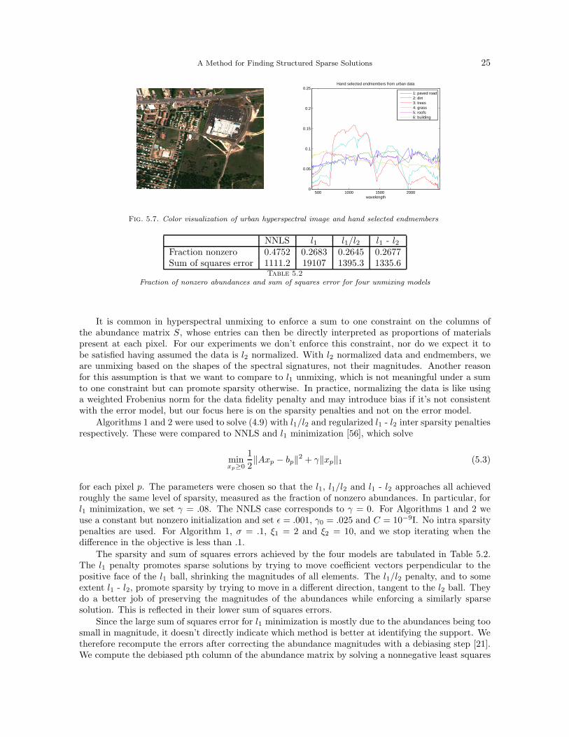
187×94249 represents the spectral signaturemeasured at a pixel in the 307 by 307 urban image shown in Figure 5.7.
The data was processed to remove some wavelengths for which the data was corrupted, resultingin a spectral resolution reduced from 210 to 187. The six endmembers forming the columns of thedictionary A were selected by hand from pixels that appeared to be pure materials. These are alsoshown in Figure 5.7. The columns of both A and Y were normalized to have unit l2 norm.
A Method for Finding Structured Sparse Solutions 25
500 1000 1500 20000
0.05
0.1
0.15
0.2
0.25
wavelength
Hand selected endmembers from urban data
1: paved road2: dirt3: trees4: grass5: roofs6: building
Fig. 5.7. Color visualization of urban hyperspectral image and hand selected endmembers
NNLS l1 l1/l2 l1 - l2Fraction nonzero 0.4752 0.2683 0.2645 0.2677Sum of squares error 1111.2 19107 1395.3 1335.6
Table 5.2
Fraction of nonzero abundances and sum of squares error for four unmixing models
It is common in hyperspectral unmixing to enforce a sum to one constraint on the columns ofthe abundance matrix S, whose entries can then be directly interpreted as proportions of materialspresent at each pixel. For our experiments we don’t enforce this constraint, nor do we expect it tobe satisfied having assumed the data is l2 normalized. With l2 normalized data and endmembers, weare unmixing based on the shapes of the spectral signatures, not their magnitudes. Another reasonfor this assumption is that we want to compare to l1 unmixing, which is not meaningful under a sumto one constraint but can promote sparsity otherwise. In practice, normalizing the data is like usinga weighted Frobenius norm for the data fidelity penalty and may introduce bias if it’s not consistentwith the error model, but our focus here is on the sparsity penalties and not on the error model.
Algorithms 1 and 2 were used to solve (4.9) with l1/l2 and regularized l1 - l2 inter sparsity penaltiesrespectively. These were compared to NNLS and l1 minimization [56], which solve
minxp≥0
1
2‖Axp − bp‖2 + γ‖xp‖1 (5.3)
for each pixel p. The parameters were chosen so that the l1, l1/l2 and l1 - l2 approaches all achievedroughly the same level of sparsity, measured as the fraction of nonzero abundances. In particular, forl1 minimization, we set γ = .08. The NNLS case corresponds to γ = 0. For Algorithms 1 and 2 weuse a constant but nonzero initialization and set ǫ = .001, γ0 = .025 and C = 10−9I. No intra sparsitypenalties are used. For Algorithm 1, σ = .1, ξ1 = 2 and ξ2 = 10, and we stop iterating when thedifference in the objective is less than .1.
The sparsity and sum of squares errors achieved by the four models are tabulated in Table 5.2.The l1 penalty promotes sparse solutions by trying to move coefficient vectors perpendicular to thepositive face of the l1 ball, shrinking the magnitudes of all elements. The l1/l2 penalty, and to someextent l1 - l2, promote sparsity by trying to move in a different direction, tangent to the l2 ball. Theydo a better job of preserving the magnitudes of the abundances while enforcing a similarly sparsesolution. This is reflected in their lower sum of squares errors.
Since the large sum of squares error for l1 minimization is mostly due to the abundances being toosmall in magnitude, it doesn’t directly indicate which method is better at identifying the support. Wetherefore recompute the errors after correcting the abundance magnitudes with a debiasing step [21].We compute the debiased pth column of the abundance matrix by solving a nonnegative least squares
26 E. Esser, Y. Lou and J. Xin
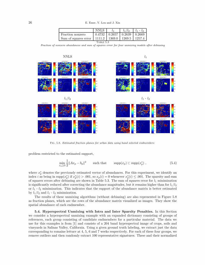
NNLS l1 l1/l2 l1 - l2Fraction nonzero 0.4732 0.2657 0.2639 0.2669Sum of squares error 1111.2 1369.0 1269.5 1257.4
Table 5.3
Fraction of nonzero abundances and sum of squares error for four unmixing models after debiasing
NNLS l1endmember 1
0
0.2
0.4
0.6
0.8
1endmember 2
0
0.2
0.4
0.6
0.8
1endmember 3
0
0.2
0.4
0.6
0.8
1
endmember 4
0
0.2
0.4
0.6
0.8
1endmember 5
0
0.2
0.4
0.6
0.8
1endmember 6
0
0.2
0.4
0.6
0.8
1
endmember 1
0
0.2
0.4
0.6
0.8
1endmember 2
0
0.2
0.4
0.6
0.8
1endmember 3
0
0.2
0.4
0.6
0.8
1
endmember 4
0
0.2
0.4
0.6
0.8
1endmember 5
0
0.2
0.4
0.6
0.8
1endmember 6
0
0.2
0.4
0.6
0.8
1
l1/l2 l1 - l2endmember 1
0
0.2
0.4
0.6
0.8
1endmember 2
0
0.2
0.4
0.6
0.8
1endmember 3
0
0.2
0.4
0.6
0.8
1
endmember 4
0
0.2
0.4
0.6
0.8
1endmember 5
0
0.2
0.4
0.6
0.8
1endmember 6
0
0.2
0.4
0.6
0.8
1
endmember 1
0
0.2
0.4
0.6
0.8
1endmember 2
0
0.2
0.4
0.6
0.8
1endmember 3
0
0.2
0.4
0.6
0.8
1
endmember 4
0
0.2
0.4
0.6
0.8
1endmember 5
0
0.2
0.4
0.6
0.8
1endmember 6
0
0.2
0.4
0.6
0.8
1
Fig. 5.8. Estimated fraction planes for urban data using hand selected endmembers
problem restricted to the estimated support,
minxp≥0
1
2‖Axp − bp‖2 such that supp(xp) ⊂ supp(x∗
p) , (5.4)
where x∗p denotes the previously estimated vector of abundances. For this experiment, we identify an
index i as being in supp(x∗p) if x
∗p(i) > .001, so xp(i) = 0 whenever x∗
p(i) ≤ .001. The sparsity and sumof squares errors after debiasing are shown in Table 5.3. The sum of squares error for l1 minimizationis significantly reduced after correcting the abundance magnitudes, but it remains higher than for l1/l2or l1 - l2 minimization. This indicates that the support of the abundance matrix is better estimatedby l1/l2 and l1 - l2 minimization.
The results of these unmixing algorithms (without debiasing) are also represented in Figure 5.8as fraction planes, which are the rows of the abundance matrix visualized as images. They show thespatial abundance of each endmember.
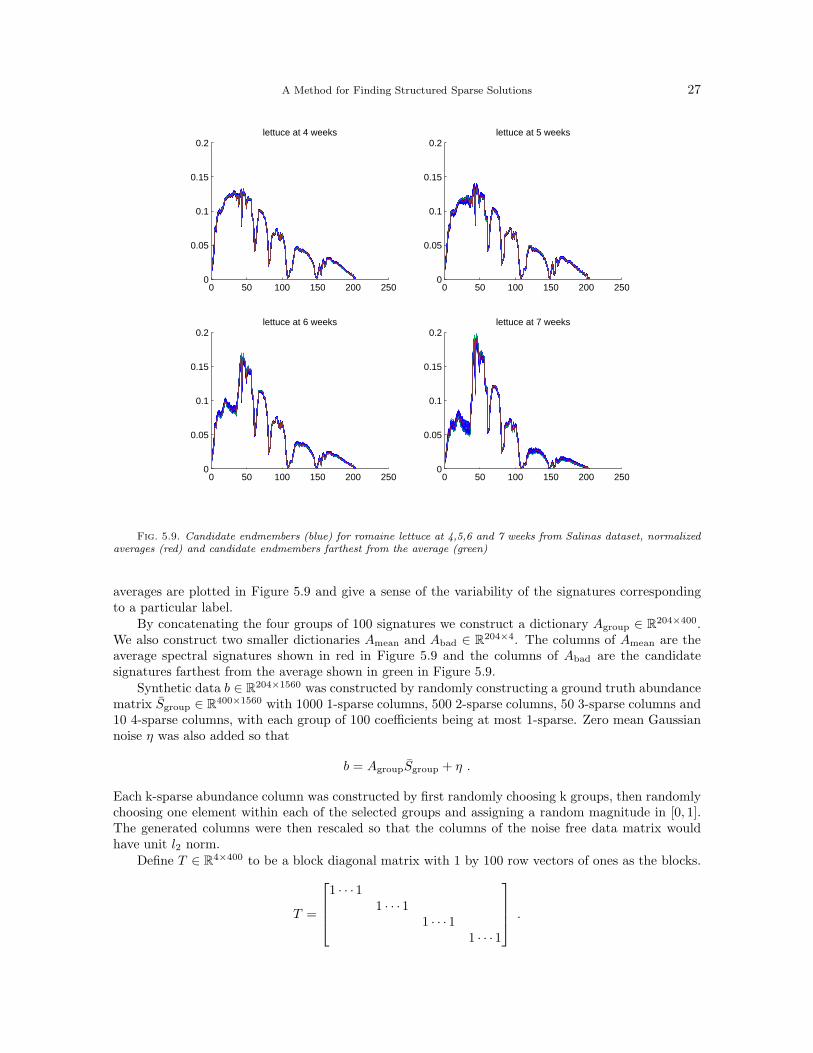
5.4. Hyperspectral Unmixing with Intra and Inter Sparsity Penalties. In this Sectionwe consider a hyperspectral unmixing example with an expanded dictionary consisting of groups ofreferences, each group consisting of candidate endmembers for a particular material. The data weuse for this examples is from [1] and consists of a 204 band hyperspectral image of crops, soils andvineyards in Salinas Valley, California. Using a given ground truth labeling, we extract just the datacorresponding to romaine lettuce at 4, 5, 6 and 7 weeks respectively. For each of these four groups, weremove outliers and then randomly extract 100 representative signatures. These and their normalized
A Method for Finding Structured Sparse Solutions 27
0 50 100 150 200 2500
0.05
0.1
0.15
0.2lettuce at 4 weeks
0 50 100 150 200 2500
0.05
0.1
0.15
0.2lettuce at 5 weeks
0 50 100 150 200 2500
0.05
0.1
0.15
0.2lettuce at 6 weeks
0 50 100 150 200 2500
0.05
0.1
0.15
0.2lettuce at 7 weeks
Fig. 5.9. Candidate endmembers (blue) for romaine lettuce at 4,5,6 and 7 weeks from Salinas dataset, normalizedaverages (red) and candidate endmembers farthest from the average (green)
averages are plotted in Figure 5.9 and give a sense of the variability of the signatures correspondingto a particular label.
By concatenating the four groups of 100 signatures we construct a dictionary Agroup ∈ R204×400.
We also construct two smaller dictionaries Amean and Abad ∈ R204×4. The columns of Amean are the
average spectral signatures shown in red in Figure 5.9 and the columns of Abad are the candidatesignatures farthest from the average shown in green in Figure 5.9.
Synthetic data b ∈ R204×1560 was constructed by randomly constructing a ground truth abundance
matrix S̄group ∈ R400×1560 with 1000 1-sparse columns, 500 2-sparse columns, 50 3-sparse columns and
10 4-sparse columns, with each group of 100 coefficients being at most 1-sparse. Zero mean Gaussiannoise η was also added so that
b = AgroupS̄group + η .
Each k-sparse abundance column was constructed by first randomly choosing k groups, then randomlychoosing one element within each of the selected groups and assigning a random magnitude in [0, 1].The generated columns were then rescaled so that the columns of the noise free data matrix wouldhave unit l2 norm.
Define T ∈ R4×400 to be a block diagonal matrix with 1 by 100 row vectors of ones as the blocks.
T =
1 · · · 11 · · · 1
1 · · · 11 · · · 1
.
28 E. Esser, Y. Lou and J. Xin
0 500 1000 15000
1
2
3
4
5NNLS
0 500 1000 15000
1
2
3
4
5l1
0 500 1000 15000
1
2
3
4
5l1l2
0 500 1000 15000
1
2
3
4
5l1−l2
0 500 1000 15000
1
2
3
4
5NNLS
0 500 1000 15000
1
2
3
4
5l1
0 500 1000 15000
1
2
3
4
5l1l2
0 500 1000 15000
1
2
3
4
5l1−l2
0 500 1000 15000
1
2
3
4
5NNLS
0 500 1000 15000
1
2
3
4
5l1
0 500 1000 15000
1
2
3
4
5l1l2
0 500 1000 15000
1
2
3
4
5l1−l2
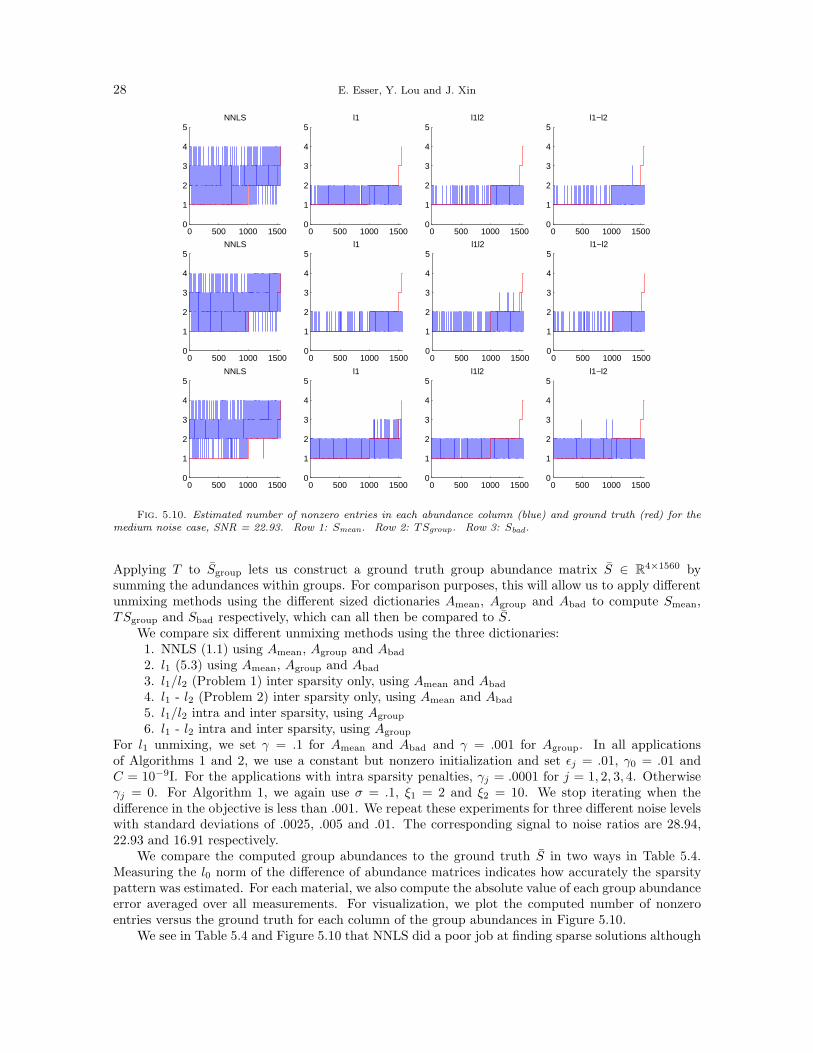
Fig. 5.10. Estimated number of nonzero entries in each abundance column (blue) and ground truth (red) for themedium noise case, SNR = 22.93. Row 1: Smean. Row 2: TSgroup. Row 3: Sbad.
Applying T to S̄group lets us construct a ground truth group abundance matrix S̄ ∈ R4×1560 by
summing the adundances within groups. For comparison purposes, this will allow us to apply differentunmixing methods using the different sized dictionaries Amean, Agroup and Abad to compute Smean,TSgroup and Sbad respectively, which can all then be compared to S̄.
We compare six different unmixing methods using the three dictionaries:1. NNLS (1.1) using Amean, Agroup and Abad
2. l1 (5.3) using Amean, Agroup and Abad
3. l1/l2 (Problem 1) inter sparsity only, using Amean and Abad
4. l1 - l2 (Problem 2) inter sparsity only, using Amean and Abad
5. l1/l2 intra and inter sparsity, using Agroup
6. l1 - l2 intra and inter sparsity, using Agroup
For l1 unmixing, we set γ = .1 for Amean and Abad and γ = .001 for Agroup. In all applicationsof Algorithms 1 and 2, we use a constant but nonzero initialization and set ǫj = .01, γ0 = .01 andC = 10−9I. For the applications with intra sparsity penalties, γj = .0001 for j = 1, 2, 3, 4. Otherwiseγj = 0. For Algorithm 1, we again use σ = .1, ξ1 = 2 and ξ2 = 10. We stop iterating when thedifference in the objective is less than .001. We repeat these experiments for three different noise levelswith standard deviations of .0025, .005 and .01. The corresponding signal to noise ratios are 28.94,22.93 and 16.91 respectively.
We compare the computed group abundances to the ground truth S̄ in two ways in Table 5.4.Measuring the l0 norm of the difference of abundance matrices indicates how accurately the sparsitypattern was estimated. For each material, we also compute the absolute value of each group abundanceerror averaged over all measurements. For visualization, we plot the computed number of nonzeroentries versus the ground truth for each column of the group abundances in Figure 5.10.
We see in Table 5.4 and Figure 5.10 that NNLS did a poor job at finding sparse solutions although
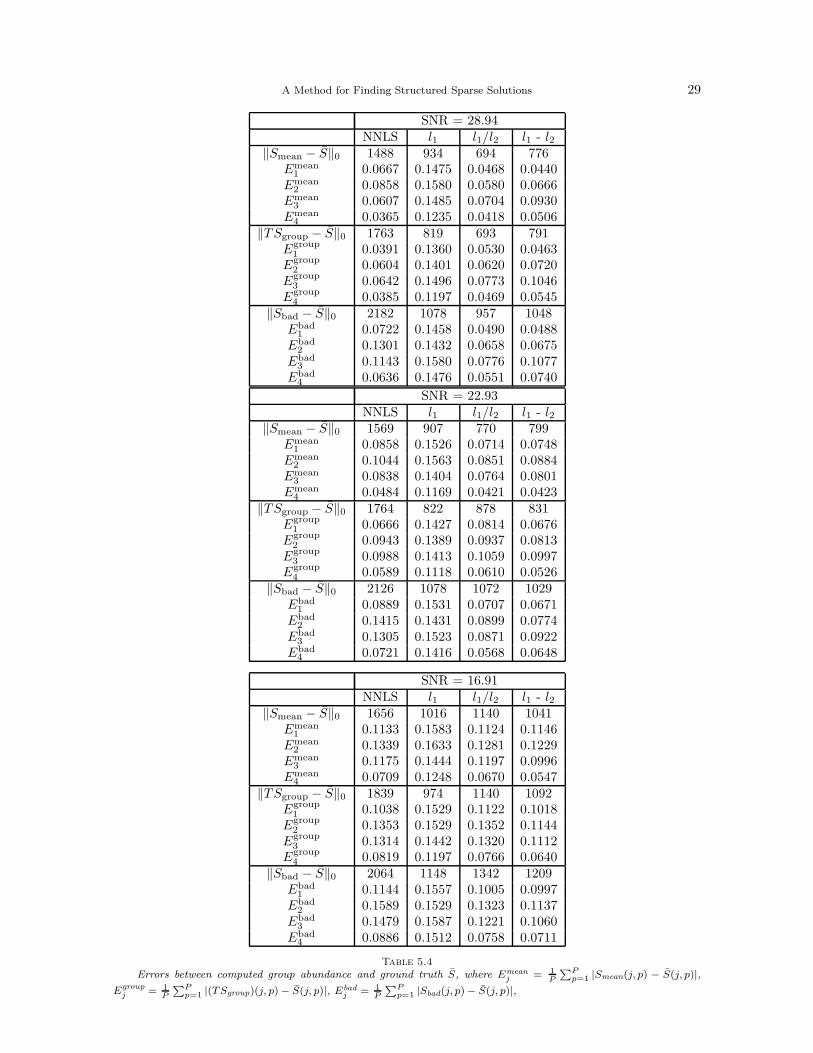
A Method for Finding Structured Sparse Solutions 29
SNR = 28.94NNLS l1 l1/l2 l1 - l2
‖Smean − S̄‖0 1488 934 694 776Emean
1 0.0667 0.1475 0.0468 0.0440Emean
2 0.0858 0.1580 0.0580 0.0666Emean
3 0.0607 0.1485 0.0704 0.0930Emean
4 0.0365 0.1235 0.0418 0.0506‖TSgroup − S̄‖0 1763 819 693 791
Egroup1 0.0391 0.1360 0.0530 0.0463
Egroup2 0.0604 0.1401 0.0620 0.0720
Egroup3 0.0642 0.1496 0.0773 0.1046
Egroup4 0.0385 0.1197 0.0469 0.0545
‖Sbad − S̄‖0 2182 1078 957 1048Ebad
1 0.0722 0.1458 0.0490 0.0488Ebad
2 0.1301 0.1432 0.0658 0.0675Ebad
3 0.1143 0.1580 0.0776 0.1077Ebad
4 0.0636 0.1476 0.0551 0.0740
SNR = 22.93NNLS l1 l1/l2 l1 - l2
‖Smean − S̄‖0 1569 907 770 799Emean
1 0.0858 0.1526 0.0714 0.0748Emean
2 0.1044 0.1563 0.0851 0.0884Emean
3 0.0838 0.1404 0.0764 0.0801Emean
4 0.0484 0.1169 0.0421 0.0423‖TSgroup − S̄‖0 1764 822 878 831
Egroup1 0.0666 0.1427 0.0814 0.0676
Egroup2 0.0943 0.1389 0.0937 0.0813
Egroup3 0.0988 0.1413 0.1059 0.0997
Egroup4 0.0589 0.1118 0.0610 0.0526
‖Sbad − S̄‖0 2126 1078 1072 1029Ebad
1 0.0889 0.1531 0.0707 0.0671Ebad
2 0.1415 0.1431 0.0899 0.0774Ebad
3 0.1305 0.1523 0.0871 0.0922Ebad
4 0.0721 0.1416 0.0568 0.0648
SNR = 16.91NNLS l1 l1/l2 l1 - l2
‖Smean − S̄‖0 1656 1016 1140 1041Emean
1 0.1133 0.1583 0.1124 0.1146Emean
2 0.1339 0.1633 0.1281 0.1229Emean
3 0.1175 0.1444 0.1197 0.0996Emean
4 0.0709 0.1248 0.0670 0.0547‖TSgroup − S̄‖0 1839 974 1140 1092
Egroup1 0.1038 0.1529 0.1122 0.1018
Egroup2 0.1353 0.1529 0.1352 0.1144
Egroup3 0.1314 0.1442 0.1320 0.1112
Egroup4 0.0819 0.1197 0.0766 0.0640
‖Sbad − S̄‖0 2064 1148 1342 1209Ebad
1 0.1144 0.1557 0.1005 0.0997Ebad
2 0.1589 0.1529 0.1323 0.1137Ebad
3 0.1479 0.1587 0.1221 0.1060Ebad
4 0.0886 0.1512 0.0758 0.0711
Table 5.4
Errors between computed group abundance and ground truth S̄, where Emeanj = 1
P
∑Pp=1
|Smean(j, p) − S̄(j, p)|,
Egroupj = 1
P
∑Pp=1
|(TSgroup)(j, p)− S̄(j, p)|, Ebadj = 1
P
∑Pp=1
|Sbad(j, p)− S̄(j, p)|,
30 E. Esser, Y. Lou and J. Xin
average coefficient errors were low. On the other hand, l1 minimization did a good job of finding asparse solution, but coefficient errors were higher because the abundance magnitudes were underesti-mated. The l1
l2and l1 − l2 minimization approaches were better at encouraging sparse solutions while
maintaining small average errors in the abundance coefficients.For this example, the average signatures used in Amean turned out to be good choices for the
endmembers, and we didn’t see any improvement in the estimated group abundances by consideringthe expanded dictionary Agroup. However, compared to using the four poorly selected endmembercandidates in Abad, we got better results with the expanded dictionary. In the expanded dictionarycase, which resulted in an underdetermined dictionary matrix, the abundances Sgroup directly computedby l1 minimization were much less sparse than those computed by l1
l2and l1 − l2 minimization. This
is because l1l2
and l1 − l2 minimization were able to enforce 1-sparsity within coefficient groups, butl1 was not. If the group 1-sparsity requirement is important for the model to be accurate, then thisis an advantage of using the l1
l2and l1 − l2 penalties. Here, this difference in sparsity turned out
not to have much effect on the group abundances TSgroup, which were computed by summing theabundances within each group. This may not hold in situations where the endmember variability ismore nonlinear. For example, if the endmember variability had to do with misalignment, as with theearlier DOAS example, then linear combinations of misaligned signatures would not produce a goodreference signature.
6. Conclusions and Future Work . We proposed a method for linear unmixing problemswhere the dictionary contains multiple references for each material and we want to collaborativelychoose the best one for each material present. More generally, we showed how to use l1
l2and l1 − l2
penalties to obtain structured sparse solutions to non-negative least squares problems. These werereformulated as constrained minimization problems with differentiable but non-convex objectives. Ascaled gradient projection method based on difference of convex programming was proposed. Thisapproach requires solving a sequence of strongly quadratic programs, and we showed how these canbe efficiently solved using the alternating direction method of multipliers. Moreover, few iterationswere required in practice, between 4 and 20 for all the numerical examples presented in this paper.Some convergence analysis was also presented to show that limit points of the iterates are stationarypoints. Numerical results for unmixing problems in differential optical absorption spectroscopy andhyperspectral image analysis show that our difference of convex approach using l1
l2and l1− l2 penalties
is capable of promoting different levels of sparsity on possibly overlapping subsets of the fitting orabundance coefficients.
For future work we would like to test this method on more general multiple choice quadraticknapsack problems, which are related to the applications presented here that focused on finding so-lutions that were at most 1-sparse within specified groups. It would be interesting to see how thisvariational approach performs relative to combinatorial optimization strategies for similar problems.We are also interested in exploring alternative sparsity penalties that can be adapted to the data set.When promoting 1-sparse solutions, the experiments in this paper used fixed sparsity parameters thatwere simply chosen to be sufficiently large. We are interested in justifying the technique of graduallyincreasing this parameter while iterating, which empirically seems better able to avoid bad local min-ima. The applications presented here all involved uncertainty in the dictionary, which was expandedto include multiple candidate references for each material. If a-priori assumptions are available aboutthe relative likelihood of these candidates, we would like to incorporate this into the model.
Acknowledgments - We thank Lisa Wingen for providing DOAS references and data, which we usedas a guide when generating synthetic data for some of our numerical examples. Thanks to John Greerfor pointing out a paper by A. Zare and P. Gader [67]. We would also like to thank the anonymousreferees for their constructive comments.
A Method for Finding Structured Sparse Solutions 31
REFERENCES
[1] Salinas aviris dataset. Available online at http://www.ehu.es/ccwintco/index.php/Hyperspectral_Remote_
Sensing_Scenes.[2] Urban dataset. US Army Corps of Engineers. Freely available online at www.tec.army.mil/hypercube.[3] Richard G Baraniuk, Volkan Cevher, Marco F Duarte, and Chinmay Hegde, Model-based compressive
sensing, Information Theory, IEEE Transactions on, 56 (2010), pp. 1982–2001.[4] M. Berry, M. Browne, A. Langville, P. Pauca, and R.J. Plemmons, Algorithms and applications for approx-
imate nonnegative matrix factorization, Computational Statistics and Data Analysis, 52 (2007), pp. 155–173.[5] A. L. Bertozzi, S. Esedoglu, and A. Gillette, Analysis of a two-scale Cahn-Hilliard model for image inpainting,
Multiscale Modeling and Simulation, 6 (2007), pp. 913–936.[6] D. Bertsekas, Nonlinear Programming, Athena Scientific, 1999.[7] D. Bertsekas and J. Tsitsiklis, Parallel and Distributed Computation, Prentice Hall, 1989.[8] J. M. Bioucas-Dias, A. Plaza, N. Dobigeon, M. Parente, Q. Du, P. Gader, and J. Chanussot, Hyperspectral
unmixing overview: Geometrical, statistical, and sparse regression-based approaches, IEEE Trans. Imag. Proc.,5 (2012), pp. 354–379.
[9] S. Bonettini, R. Zanella, and L. Zanni, A scaled gradient projection method for constrained image deblurring,Inverse problems, 25 (2009). 015002.
[10] Peter Brucker, An o(n) algorithm for quadratic knapsack problems, Operations Research Letters, 3 (1984),pp. 163–166.
[11] A. M. Bruckstein, M. Elad, and M. Zibulevsky, On the uniqueness of nonnegative sparse solutions to under-determined systems of equations, Information Theory, IEEE Transactions on, 54 (2008), pp. 4813 –4820.
[12] E. Candes, J. Romberg, and T. Tao, Stable signal recovery from incomplete and inaccurate measurements,Comm. Pure Appl. Math., 59 (2006), pp. 1207–1223.
[13] A. Castrodad, Z. Xing, J. Greer, E. Bosch, L. Carin, and G. Sapiro, Learning discriminativesparse models for source separation and mapping of hyperspectral imagery. Submitted September 2010,http://www.ima.umn.edu/preprints/oct2010/oct2010.html.
[14] A. Chambolle and T. Pock, A first-order primal-dual algorithm for convex problems with applications to imaging,Journal of Mathematical Imaging and Vision, 40 (2011).
[15] Scott Shaobing Chen, David L. Donoho, and Michael A. Saunders, Atomic decomposition by basis pursuit,SIAM Journal on Scientific Computing, 20 (1998), pp. 33–61.
[16] O. Eches, N. Dobigeon, C. Mailhes, and J.-Y. Tourneret, Bayesian estimation of linear mixtures using thenormal compositional model. application to hyperspectral imagery, IEEE Trans. Image Process., 19 (2010),pp. 1403–1413.
[17] M. T. Eismann and D. Stein, Stochastic mixture modeling, in Hyperspectral Data Exploitation: Theory andApplications, C.-I Chang, ed., Wiley, 2007.
[18] E. Esser, M. Moller, S. Osher, G. Sapiro, and J. Xin, A convex model for nonnegative matrix factorizationand dimensionality reduction on physical space, IEEE Trans. Imag. Proc., 21 (2012), pp. 3239–3252.
[19] E. Esser, X. Zhang, and T.F. Chan, A general framework for a class of first order primal-dual algorithms forconvex optimization in imaging science, SIAM J. Imaging Sci., 3 (2010), pp. 1015–1046.
[20] D. Eyre, An unconditionally stable one-step scheme for gradient systems, 1998.www.math.utah.edu/ eyre/research/methods/stable.ps.
[21] M. Figueiredo, R. Nowak, and S. Wright, Gradient projection for sparse reconstruction: Application to com-pressed sensing and other inverse problems, IEEE Journal of Selected Topics in Signal Processing, 1 (2007),pp. 586–597.
[22] Finlayson-Pitts, Unpublished data. Provided by Lisa Wingen, 2000.[23] J. Friedman, T. Hastie, and R. Tibshirani, A note on the group lasso and a sparse group lasso, tech. report,
2010. Stanford Department of Statistics.[24] D. Gabay and B. Mercier, A dual algorithm for the solution of nonlinear variational problems via finite-element
approximations, Comp. Math. Appl., 2 (1976), pp. 17–40.[25] R. Glowinski and A. Marrocco, Sur lapproximation par elements finis dordre un, et la resolution par
penalisation-dualite dune classe de problemes de Dirichlet nonlineaires, Rev. Francaise dAut Inf. Rech. Oper.,R-2 (1975), pp. 41–76.
[26] T. Goldstein and S. Osher, The split bregman method for l1-regularized problems, SIAM Journal on ImagingScience, 2 (2009), pp. 323–343.
[27] J. Greer, Sparse demixing, SPIE proceedings on Algorithms and Technologies for Multispectral, Hyperspectral,and Ultraspectral Imagery XVI, 7695 (2010), pp. 76951O–76951O–12.
[28] Z. Guo and S. Osher, Template matching via l1 minimization and its application to hyperspectral data, InverseProblems Imaging, 1 (2011), pp. 19–35.
[29] Z. Guo, T. Wittman, and S. Osher, L1 unmixing and its application to hyperspectral image enhancement, Pro-ceedings SPIE Conference on Algorithms and Technologies for Multispectral, Hyperspectral, and UltraspectralImagery XV, 7334 (2008), pp. 73341M–73341M–9.
[30] P. O. Hoyer, Non-negative sparse coding, in Proc. IEEE Workshop on Neural Networks for Signal Processing,2002. pages 557-565.
[31] , Non-negative matrix factorization with sparseness constraints, Journal of Machine Learning Research, 5
32 E. Esser, Y. Lou and J. Xin
(2004), pp. 1457–1469.[32] Y. H. Hu, H. B. Lee, and F. L. Scarpace, Optimal linear spectral unmixing, Geoscience and Remote Sensing,
IEEE Transactions on, 37 (1999), pp. 639 –644.[33] Junzhou Huang, Tong Zhang, and Dimitris Metaxas, Learning with structured sparsity, The Journal of Machine
Learning Research, 12 (2011), pp. 3371–3412.[34] N. Hurley and S. Rickard, Comparing measures of sparsity, IEEE Transactions on Information Theory, 55
(2009), pp. 4723–4741.[35] M. D. Iordache, J. M. Bioucas-Dias, and A. Plaza, Sparse unmixing of hyperspectral data, Geoscience and
Remote Sensing, IEEE Transactions on, 49 (2011), pp. 2014 –2039.[36] R. Jenatton, J.-Y. Audibert, and F. Bach, Structured variable selection with sparsity-inducing norms, tech.
report, 2010. arXiv:0904.3523v3.[37] R. Jenatton, G. Obozinski, and F. Bach, Structured sparse principal component analysis, in International
Conference on Artificial Intelligence and Statistics (AISTATS), 2010.[38] H. Ji, J. Li, Z. Shen, and K. Wang, Image deconvolution using a characterization of sharp images in wavelet
domain, Applied and Computational Harmonic Analysis, 32 (2012), pp. 295–304.[39] N. Keshava and J.F. Mustard, Spectral unmixing, Signal Processing Magazine, IEEE, 19 (2002), pp. 44 –57.[40] D. Krishnan, T. Tay, and R. Fergus, Blind deconvolution using a normalized sparsity measure, in CVPR, 2011.[41] K. Lange, D. Hunter, and I. Yang, Optimization transfer using surrogate objective functions, Journal of Com-
putational and Graphical Statistics, 9 (2000), pp. 1–20.[42] C.L. Lawson and R.J. Hanson, Solving Least Squares Problems, Prentice-Hall: Englewood Cliffs, NJ, 1974.[43] D. D. Lee and H. S. Seung, Algorithms for non-negative matrix factorization, in Proc. NIPS, Advances in Neural
Information Processing 13, 2001.[44] Y. Lou, A. L. Bertozzi, and S. Soatto, Direct sparse deblurring, Journal of Mathematical Imaging and Vision,
39 (2011), pp. 1–12.[45] Zhaosong Lu and Yong Zhang, Penalty decomposition methods for L0-norm minimization, arXiv:1008.5372v2,
(2012).[46] Julien Mairal, Francis Bach, Jean Ponce, and Guillermo Sapiro, Online dictionary learning for sparse
coding, in Proceedings of the 26th Annual International Conference on Machine Learning, ICML ’09, NewYork, NY, USA, 2009, ACM, pp. 689–696.
[47] L. Meier, S. van de Geer, and P. Buhlmann, The group lasso for logistic regression, J. R. Statist. Soc. B, 70(2008), pp. 53–71.
[48] J. M. P. Nascimento and J. M. Bioucas-Dias, Vertex component analysis: A fast algorithm to unmix hyper-spectral data, IEEE Trans. Geosci. Rem. Sens., 43 (2004), pp. 898–910.
[49] V. P. Pauca, J. Piper, and R. J. Plemmons, Nonnegative matrix factorization for spectral data analysis, LinearAlgebra and its Applications, 416 (2006), pp. 29–47.
[50] U. Platt and J. Stutz, Differential Optical Absorption Spectroscopy: Principles and Applications, Springer,2008.
[51] Z. Qin and D. Goldfarb, Structured sparsity via alternating direction methods, The Journal of Machine LearningResearch, 98888 (2012), pp. 1435–1468.
[52] N. Saito and J-F. Remy, The polyharmonic local sine transform: A new tool for local image analysis and synthesiswithout edge effect, Applied and Computational Harmonic Analysis, 20 (2006), pp. 41–73.
[53] M. Slawski and M. Hein, Sparse recovery by thresholded non-negative least squares, in NIPS, 2011.[54] B. Sriperumbudur and G. Lanckriet, On the convergence of the concave-convex procedure, in NIPS, 2009.[55] D. Stein, Application of the normal compositional model to the analaysis of hyperspectral imagery, in IEEE
Workshop on Advances in Techniques for Analysis of Remotely Sensed Data, Oct. 2003, pp. 44–51.[56] A. Szlam, Z. Guo, and S. Osher, A split Bregman method for non-negative sparsity penalized least squares
with applications to hyperspectral demixing, in International Conference on Image Processing (ICIP), 2010,pp. 1917–1920.
[57] Pham Dinh Tao and Le Thi Hoai An, Convex analysis approach to d.c. programming: Theory, algorithms andapplications, Acta Mathematica Vietnamica, 22 (1997), pp. 289–355.
[58] , A d.c. optimization algorithm for solving the trust-region subproblem, SIAM J. Optim., 8 (1998), pp. 476–505.
[59] Robert Tibshirani, Regression shrinkage and selection via the lasso, Journal of the Royal Statistical Society.Series B (Methodological), 58 (1996), pp. pp. 267–288.
[60] J. A. Tropp, Greed is good: algorithmic results for sparse approximation, Information Theory, IEEE Transactionson, 50 (2004), pp. 2231 – 2242.
[61] B. P. Vollmayr-Lee and A. D. Rutenberg, Fast and accurate coarsening simulation with an unconditionallystable time step, Phys. Rev. E, 68 (2003), pp. 1–13.
[62] M. E. Winter, N-FINDR: an algorithm for fast autonomous spectral end-member determination in hyperspectraldata, in Imaging Spectrometry V, vol. 3753, SPIE, 1999, pp. 266–275.
[63] Wotao Yin, Stanley Osher, Donald Goldfarb, and Jerome Darbon, Bregman iterative algorithms forl1minimization with applications to compressed sensing, SIAM J. Imaging Sci, 1 (2008), pp. 143–168.
[64] M. Yuan and Y. Lin, Model selection and estimation in regression with grouped variables, Journal of the RoyalStatistical Society, Series B, 68 (2007), pp. 49–67.
[65] A. Yuille and A. Rangarajan, The concave-convex procedure, Neural Computation, 15 (2003), pp. 915–936.

A Method for Finding Structured Sparse Solutions 33
[66] A. Zare, Hyperspectral endmember detection and band selection using Bayesian methods, 2008.http://gradworks.umi.com/33/47/3347194.html.
[67] A. Zare and P. Gader, PCE: Piece-wise convex endmember detection, IEEE Transactions on Geoscience andRemote Sensing, 48 (2010), pp. 2620–2632.
[68] Y. Zhou, R. Jin, and S.C. Hoi, Exclusive lasso for multi-task feature selection, in In AISTATS, 2010.