Embed Size (px)
Citation preview

A Memetic Genetic Program for KnowledgeDiscovery
by
Gert Nel
Submitted in partial fulfilment of the requirements for the degree
Master of Science
in the Faculty of Engineering, Built Environment and Information Technology
University of Pretoria
Pretoria
December 2004
UUnniivveerrssiittyy ooff PPrreettoorriiaa eettdd –– NNeell,, GG MM ((22000055))
A Memetic Genetic Program for Knowledge Discovery
by
Gert Nel
Abstract
Local search algorithms have been proved to be effective in refining solutions that have been
found by other algorithms. Evolutionary algorithms, in particular global search algorithms,
have shown to be successful in producing approximate solutions for optimisation and
classification problems in acceptable computation times. A relatively new method, memetic
algorithms, uses local search to refine the approximate solutions produced by global search
algorithms. This thesis develops such a memetic algorithm. The global search algorithm used
as part of the new memetic algorithm is a genetic program that implements the building block
hypothesis by building simplistic decision trees representing valid solutions, and gradually
increases the complexity of the trees. The specific building block hypothesis implementation
is known as the building block approach to genetic programming, BGP. The effectiveness and
efficiency of the new memetic algorithm, which combines the BGP algorithm with a local
search algorithm, is demonstrated.
Keywords: Evolutionary algorithms, memetic algorithms, building block hypothesis, global
search, local search, optimisation, classification problems, genetic program, decision trees,
BGP, MBGP.
Supervisor: Prof. A. P. Engelbrecht
Department of Computer Science
Degree: Master of Science
UUnniivveerrssiittyy ooff PPrreettoorriiaa eettdd –– NNeell,, GG MM ((22000055))

Contents
1 Introduction 1
1.1 Problem Statement and Overview . . . . . . . . . . . . . . . . . . . . . . . 1
1.2 Thesis Objectives . . . . . . . . . . . . . . . . . . . . . . . . . . . . . . . . 2
1.3 Thesis Contribution . . . . . . . . . . . . . . . . . . . . . . . . . . . . . . 3
1.4 Thesis Outline . . . . . . . . . . . . . . . . . . . . . . . . . . . . . . . . . 4
2 Background & Literature Study 6
2.1 Optimisation and Classification . . . . . . . . . . . . . . . . . . . . . . . . 6
2.1.1 Search Paradigms . . . . . . . . . . . . . . . . . . . . . . . . . . . 8
2.2 Evolutionary Computation . . . . . . . . . . . . . . . . . . . . . . . . . . . 11
2.3 Evolutionary Algorithms . . . . . . . . . . . . . . . . . . . . . . . . . . . . 13
2.3.1 Benefits and General Architecture . . . . . . . . . . . . . . . . . . 14
2.3.2 Initial Population . . . . . . . . . . . . . . . . . . . . . . . . . . . . 16
2.3.3 Representation of the Genotype . . . . . . . . . . . . . . . . . . . . 17
2.3.4 Evolutionary Operators . . . . . . . . . . . . . . . . . . . . . . . . 17
2.3.5 Recombination . . . . . . . . . . . . . . . . . . . . . . . . . . . . . 18
2.3.6 Mutation . . . . . . . . . . . . . . . . . . . . . . . . . . . . . . . . 19
2.3.7 Selection . . . . . . . . . . . . . . . . . . . . . . . . . . . . . . . . 20
2.3.8 Issues in EA . . . . . . . . . . . . . . . . . . . . . . . . . . . . . . 22
2.4 Rule Extraction . . . . . . . . . . . . . . . . . . . . . . . . . . . . . . . . . 24
2.4.1 Motivation for Knowledge Discovery . . . . . . . . . . . . . . . . . 24
2.4.2 Knowledge Discovery . . . . . . . . . . . . . . . . . . . . . . . . . . 26
2.4.3 Rule Extraction . . . . . . . . . . . . . . . . . . . . . . . . . . . . . 29
2.5 Concluding Remarks . . . . . . . . . . . . . . . . . . . . . . . . . . . . . . 37
i
UUnniivveerrssiittyy ooff PPrreettoorriiaa eettdd –– NNeell,, GG MM ((22000055))

3 Genetic Programming 38
3.1 Genetic Programming for RE . . . . . . . . . . . . . . . . . . . . . . . . . 38
3.1.1 Introduction . . . . . . . . . . . . . . . . . . . . . . . . . . . . . . 38
3.1.2 Evolving a Program and Evolutionary Operators . . . . . . . . . . . 39
3.1.3 Representation of a Classification Problem and RE . . . . . . . . . 53
3.2 Building Block Approach to GP . . . . . . . . . . . . . . . . . . . . . . . . 57
3.2.1 Philosophical Motivation for the Building Block Hypothesis . . . . 57
3.2.2 Building Block Hypothesis Critique . . . . . . . . . . . . . . . . . . 59
3.2.3 General Architecture and Representation . . . . . . . . . . . . . . . 60
3.2.4 Initialisation of Population . . . . . . . . . . . . . . . . . . . . . . 62
3.2.5 Fitness Evaluation . . . . . . . . . . . . . . . . . . . . . . . . . . . 63
3.2.6 Termination Condition . . . . . . . . . . . . . . . . . . . . . . . . . 65
3.2.7 Addition of Building Blocks . . . . . . . . . . . . . . . . . . . . . . 66
3.2.8 Selection . . . . . . . . . . . . . . . . . . . . . . . . . . . . . . . . 67
3.2.9 Mutation . . . . . . . . . . . . . . . . . . . . . . . . . . . . . . . . 68
3.2.10 Pruning . . . . . . . . . . . . . . . . . . . . . . . . . . . . . . . . 69
3.2.11 Recombination . . . . . . . . . . . . . . . . . . . . . . . . . . . . 69
3.2.12 Finding the Best Individual . . . . . . . . . . . . . . . . . . . . . 69
3.3 Concluding Remarks . . . . . . . . . . . . . . . . . . . . . . . . . . . . . . 70
4 Experimental Procedure 71
4.1 Experimental Data . . . . . . . . . . . . . . . . . . . . . . . . . . . . . . . 71
4.1.1 Ionosphere Problem . . . . . . . . . . . . . . . . . . . . . . . . . . 71
4.1.2 Iris Plant Problem . . . . . . . . . . . . . . . . . . . . . . . . . . . 72
4.1.3 Monks Problems . . . . . . . . . . . . . . . . . . . . . . . . . . . . 72
4.1.4 Pima Indian Diabetes Problem . . . . . . . . . . . . . . . . . . . . 73
4.2 Experimental Procedure . . . . . . . . . . . . . . . . . . . . . . . . . . . . 74
4.3 Improving BGP Fitness Function . . . . . . . . . . . . . . . . . . . . . . . 75
4.4 Improved Fitness Function Results . . . . . . . . . . . . . . . . . . . . . . 76
4.5 Concluding Remarks . . . . . . . . . . . . . . . . . . . . . . . . . . . . . . 86
5 Local Search Methods 87
5.1 Local Search Algorithms . . . . . . . . . . . . . . . . . . . . . . . . . . . . 87
ii
UUnniivveerrssiittyy ooff PPrreettoorriiaa eettdd –– NNeell,, GG MM ((22000055))
5.2 Combining Local and Global Search . . . . . . . . . . . . . . . . . . . . . 92
5.3 Memetic Algorithms . . . . . . . . . . . . . . . . . . . . . . . . . . . . . . 95
5.3.1 Local-Search-based Memetic Algorithm . . . . . . . . . . . . . . . . 95
5.3.2 Recombination . . . . . . . . . . . . . . . . . . . . . . . . . . . . . 99
5.3.3 Mutation . . . . . . . . . . . . . . . . . . . . . . . . . . . . . . . . 101
5.3.4 Termination Condition . . . . . . . . . . . . . . . . . . . . . . . . . 102
5.4 Directed Increasing Incremental Local Search . . . . . . . . . . . . . . . . 103
5.5 Concluding Remarks . . . . . . . . . . . . . . . . . . . . . . . . . . . . . . 106
6 Extended BGP for Rule Extraction 107
6.1 Extending the BGP Algorithm . . . . . . . . . . . . . . . . . . . . . . . . . 107
6.1.1 Introduction . . . . . . . . . . . . . . . . . . . . . . . . . . . . . . 108
6.1.2 Enhanced Building Block Approach to Genetic Programming . . . 108
6.1.3 Memetic Building Block Approach to Genetic Programming . . . . 109
6.1.4 Complexity Associated with Extended Algorithms . . . . . . . . . . 112
6.1.5 Questions Raised by Extending the BGP Algorithm . . . . . . . . . 114
6.2 Experimental Results . . . . . . . . . . . . . . . . . . . . . . . . . . . . . 114
6.2.1 Iono Experiment . . . . . . . . . . . . . . . . . . . . . . . . . . . . 117
6.2.2 Iris Experiment . . . . . . . . . . . . . . . . . . . . . . . . . . . . . 127
6.2.3 Monks1 Experiment . . . . . . . . . . . . . . . . . . . . . . . . . . 133
6.2.4 Monks2 Experiment . . . . . . . . . . . . . . . . . . . . . . . . . . 138
6.2.5 Monks3 Experiment . . . . . . . . . . . . . . . . . . . . . . . . . . 146
6.2.6 Pima Experiment . . . . . . . . . . . . . . . . . . . . . . . . . . . . 152
6.2.7 Combined Observations from Experiments . . . . . . . . . . . . . 159
6.3 Concluding Remarks . . . . . . . . . . . . . . . . . . . . . . . . . . . . . . 163
7 Conclusion 164
7.1 Conclusion and Summary . . . . . . . . . . . . . . . . . . . . . . . . . . . 164
7.2 Future Research . . . . . . . . . . . . . . . . . . . . . . . . . . . . . . . . 167
Bibliography 170
iii
UUnniivveerrssiittyy ooff PPrreettoorriiaa eettdd –– NNeell,, GG MM ((22000055))
List of Figures
2.1 Rough and convoluted search space . . . . . . . . . . . . . . . . . . . . . 9
2.2 General architecture of classical EAs . . . . . . . . . . . . . . . . . . . . . 16
2.3 One-point crossover . . . . . . . . . . . . . . . . . . . . . . . . . . . . . . 18
2.4 Data instances grouped into classes by rules . . . . . . . . . . . . . . . . . 28
2.5 Two dimensional input space partitioned by a 5 � 5 fuzzy grid . . . . . . . 37
3.1 Building an expression tree . . . . . . . . . . . . . . . . . . . . . . . . . . 42
3.2 The completed expression tree . . . . . . . . . . . . . . . . . . . . . . . . 43
3.3 Grow mutation in an expression tree . . . . . . . . . . . . . . . . . . . . . 44
3.4 Swap mutation in an expression tree . . . . . . . . . . . . . . . . . . . . . 45
3.5 Trunc mutation in an expression tree . . . . . . . . . . . . . . . . . . . . . 46
3.6 One-node mutation in an expression tree . . . . . . . . . . . . . . . . . . . 47
3.7 All-node mutation in an expression tree . . . . . . . . . . . . . . . . . . . 48
3.8 One-node crossover in an expression tree . . . . . . . . . . . . . . . . . . . 50
3.9 Sub-tree crossover in an expression tree . . . . . . . . . . . . . . . . . . 52
3.10 Selection numbering of the nodes of an expression tree . . . . . . . . . . 53
3.11 Decision tree representation . . . . . . . . . . . . . . . . . . . . . . . . . 56
3.12 The original BGP algorithm . . . . . . . . . . . . . . . . . . . . . . . . . . 61
4.1 Generalised maximum and best tree fitness BGP and IFBGP . . . . . . . 80
4.2 The average tree depth of BGP and IFBGP . . . . . . . . . . . . . . . . . . 85
4.3 The average tree width of BGP and IFBGP . . . . . . . . . . . . . . . . . . 85
5.1 General framework of a LS-Based MA . . . . . . . . . . . . . . . . . . . . . 96
5.2 The (Guided) Local-Search-Engine Algorithm . . . . . . . . . . . . . . . . 99
5.3 The DIILS method . . . . . . . . . . . . . . . . . . . . . . . . . . . . . . . . 105
6.1 Local search algorithm in the EBGP algorithm . . . . . . . . . . . . . . . . 110
6.2 Local search algorithm in the MBGP algorithm . . . . . . . . . . . . . . . . 112
6.3 Iono - Comparing the BGP, EBGP and MBGP algorithms . . . . . . . . . . 119
iv
UUnniivveerrssiittyy ooff PPrreettoorriiaa eettdd –– NNeell,, GG MM ((22000055))
6.4 Iono - The average tree depth of BGP, EBGP and MBGP . . . . . . . . . . . 126
6.5 Iono - The average tree width of BGP, EBGP and MBGP . . . . . . . . . . . 126
6.6 Iris - Comparing the BGP, EBGP and MBGP algorithms . . . . . . . . . . . 128
6.7 Iris - The average tree depth of BGP, EBGP and MBGP . . . . . . . . . . . 132
6.8 Iris - The average tree width of BGP, EBGP and MBGP . . . . . . . . . . . 132
6.9 Monks1 - Comparing the BGP, EBGP and MBGP algorithms . . . . . . . . 134
6.10 Monks1 - The average tree depth of BGP, EBGP and MBGP . . . . . . . . 137
6.11 Monks1 - The average tree width of BGP, EBGP and MBGP . . . . . . . . 138
6.12 Monks2 - Comparing the BGP, EBGP and MBGP algorithms . . . . . . . 140
6.13 Monks2 - The average tree depth of BGP, EBGP and MBGP . . . . . . . . 145
6.14 Monks2 - The average tree width of BGP, EBGP and MBGP . . . . . . . . 145
6.15 Monks3 - Comparing the BGP, EBGP and MBGP algorithms . . . . . . . 148
6.16 Monks3 - The average tree depth of BGP, EBGP and MBGP . . . . . . . . 151
6.17 Monks3 - The average tree width of BGP, EBGP and MBGP . . . . . . . . 151
6.18 Pima - Comparing the BGP, EBGP and MBGP algorithms . . . . . . . . . 154
6.19 Pima - The average tree depth of BGP, EBGP and MBGP . . . . . . . . . . 158
6.20 Pima - The average tree width of BGP, EBGP and MBGP . . . . . . . . . . 158
v
UUnniivveerrssiittyy ooff PPrreettoorriiaa eettdd –– NNeell,, GG MM ((22000055))
List of Tables
4.1 The input parameters used by BGP and IFBGP . . . . . . . . . . . . . . . 77
4.2 The normalised generation mapping of Monks1 . . . . . . . . . . . . . . . 79
4.3 The rules of the best decision tree for Monks1 . . . . . . . . . . . . . . . . 82
6.1 Iono - The input parameters used by BGP, EBGP and MBGP . . . . . . . . 117
6.2 Iono - The normalised generation mapping . . . . . . . . . . . . . . . . . . 118
6.3 Iono - The rules of the best decision tree . . . . . . . . . . . . . . . . . . . 122
6.4 Iris - The input parameters used by BGP, EBGP and MBGP . . . . . . . . 127
6.5 Iris - The normalised generation mapping . . . . . . . . . . . . . . . . . . 128
6.6 Iris - The rules of the best decision tree . . . . . . . . . . . . . . . . . . . . 130
6.7 Monks1 - The input parameters used by BGP, EBGP and MBGP . . . . . . 133
6.8 Monks1 - The normalised generation mapping . . . . . . . . . . . . . . . . 133
6.9 Monks1 - The rules of the best decision tree . . . . . . . . . . . . . . . . . 136
6.10 Monks2 - The input parameters used by BGP, EBGP and MBGP . . . . . 139
6.11 Monks2 - The normalised generation mapping . . . . . . . . . . . . . . . 139
6.12 Monks2 - The rules of the best decision tree . . . . . . . . . . . . . . . . 141
6.13 Monks3 - The input parameters used by BGP, EBGP and MBGP . . . . . 146
6.14 Monks3 - The normalised generation mapping . . . . . . . . . . . . . . . 146
6.15 Monks3 - The rules of the best decision tree . . . . . . . . . . . . . . . . 149
6.16 Pima - The input parameters used by BGP, EBGP and MBGP . . . . . . . 152
6.17 Pima - The normalised generation mapping . . . . . . . . . . . . . . . . . 152
6.18 Pima - The rules of the best decision tree . . . . . . . . . . . . . . . . . . 155
vi
UUnniivveerrssiittyy ooff PPrreettoorriiaa eettdd –– NNeell,, GG MM ((22000055))

Chapter 1
Introduction
1.1 Problem Statement and Overview
Many real world problems have a requirement that the solutions which are produced should
solve particular problems with high accuracy and be provided in the shortest possible time.
Examples of such real world problems include air traffic control systems, fraud detection,
medical analysis systems, production and process control systems, voice identification,
speech recognition, image analysis, and many more applications. Solutions that are accurate
and have been optimised quickly are therefore desirable.
Currently, two competitive paradigms have been devised that solve optimisation problems,
namely local optimisation and global optimisation. The main problem with local optimisation
algorithms is that the algorithms get caught in a local optimum in the search-space of the
associated problem. Additionally, local optimisation algorithms inherently have high
computational complexity and a large dependency on problem-specific information. Global
optimisation algorithms, on the other hand, provide approximate solutions quickly, but in
general converge slowly toward the best possible solution.
Examples of local search algorithms include hill-climbing [20, 37, 60], decision trees [69,
53], neural networks trained using back propagation [43], and the conjugate gradient method
[73]. Examples of global search algorithms are landscape approximation [49], tabu search
methods [58, 54], the leapfrog algorithm [16], simulated annealing [1], rough sets [63], neural
networks not trained using the back propagation method [38, 78, 71, 72], Bayesian networks
1
UUnniivveerrssiittyy ooff PPrreettoorriiaa eettdd –– NNeell,, GG MM ((22000055))
CHAPTER 1. INTRODUCTION 2
[14, 33, 34, 16], and evolutionary algorithms [25, 37, 3, 12].
Recently, a new method for optimisation problems, memetic algorithms, have been
developed, combining global optimisation with local optimisation in such a fashion that the
two previously competitive paradigms co-operate to produce optimal solutions [6, 7, 35, 44,
49, 54, 57, 61, 65, 79]. The memetic algorithm is in essence a global search algorithm that
utilises a local search algorithm as an operator. The global search algorithm of a memetic
algorithm provides approximate solutions to the local search algorithm, which then further
refines the solutions.
One specific type of optimisation problem is the process of knowledge discovery, or rule
extraction (RE), from databases. The objective of the process is to extract a minimal set of
simplistic rules that classifies (covers) with the best possible accuracy examples in the given
database (dataset). Several global search algorithms in the EA paradigm, which effectively
classify large datasets without performing an exhaustive search, have been developed and
investigated [6, 49, 9, 1, 13, 5, 38, 16]. Examples of EA implementations used for
optimisation and classification problems are genetic algorithms (GA) [9, 59, 60, 36], genetic
programming (GP) [13, 69, 46, 24, 50], evolutionary strategy (ES) [5, 45], evolutionary
programming (EP) [6, 7, 37], co-evolution and cultural evolution (CE) [25]. In particular, this
thesis focuses on genetic programming for rule extraction. GP utilises evolutionary operators
that perform operations on tree structures which represent the individuals in a population
that have evolved over generations. Rules are extracted from the best solution found by the
GP.
In essence, the building block hypothesis (BBH) states that solutions to a problem can be
built by using building blocks which may be solutions to other related problems. The building
block approach to the genetic programming (BGP) algorithm implements the building block
hypothesis by utilising a genetic programming algorithm, and has shown to be effective in
extracting rules from datasets [68, 69]. Therefore, the ultimate goal of the BGP algorithm is to
produce simplistic tree structures that represent simple solutions to problems from which
rules can be extracted.
1.2 Thesis Objectives
The main objective of this thesis is to study the effectiveness and efficiency of combining a
UUnniivveerrssiittyy ooff PPrreettoorriiaa eettdd –– NNeell,, GG MM ((22000055))
CHAPTER 1. INTRODUCTION 3
local search algorithm with the standard BGP algorithm as an operator, thereby transforming
the standard BGP algorithm into a memetic BGP algorithm for application to rule extraction.
Although the target application area is knowledge discovery, the combination of a local search
process with the global search process of the BGP algorithm can be applied to any target
application. In addition to the main objective, the following sub-objectives can be identified:
� To improve the efficiency of the fitness function of the BGP algorithm, if possible.
� To indicate whether the building block hypothesis has an inherent flaw whereby the
hypothesis assumes that the building blocks used to build solutions have, by implication,
the best possible accuracy.
� To develop an additional algorithm that extends the standard BGP algorithm with a local
search algorithm in a simplistic manner.
� To discern formally and define the distinction between the standard BGP algorithm
extended with a local search algorithm, and the memetic BGP algorithm.
� To compare the performance of the extended BGP and memetic BGP algorithms with the
standard BGP algorithm.
1.3 Thesis Contribution
The contributions offered by this thesis are:
� The fitness function of the BGP algorithm is sufficient not to influence the comparisons
made between the different algorithms investigated.
� A proper distinction is provided between the memetic algorithm and a global search
algorithm that has been extended with a local search algorithm in a simplistic manner.
� The development of a memetic algorithm that utilises a genetic programming algorithm for
rule extraction which implements the building block hypothesis.
� The development of a local search algorithm that is used in combination with the standard
BGP algorithm.
� The conclusion that the building block hypothesis is flawed and one may not assume, by
implication, that the building blocks used have a high accuracy unless a guarantee can be
provided that they are optimal.
� The use of appropriate building blocks which have high accuracies improves the efficiency
of the evolutionary process.
UUnniivveerrssiittyy ooff PPrreettoorriiaa eettdd –– NNeell,, GG MM ((22000055))
CHAPTER 1. INTRODUCTION 4
� The conclusion that the memetic BGP algorithm substantially improves the standard BGP
algorithm, though at the cost of producing more complex rule sets which have higher
accuracies than the solutions provided with the standard BGP algorithm.
� The computational complexity of the memetic BGP algorithm is substantially higher than
that of the standard BGP algorithm.
1.4 Thesis Outline
Chapter 2 introduces the concepts of optimisation and classification. The theory of
evolutionary computation is reviewed with regard to the theory of evolution as provided by
Charles Darwin [21]. The general framework of an evolutionary algorithm is then given and
the evolutionary operators reviewed. The process of rule extraction in the context of
knowledge discovery is then discussed. An overview of the current optimisation paradigms are
then presented to familiarise the reader with existing methods.
Chapter 3 presents the genetic programming algorithm in the context of rule extraction
and elaborates on the evolutionary operators used. The building block approach to genetic
programming (BGP) is then discussed in detail.
Chapter 4 provides an overview of the test datasets used in simulations to compare the
algorithms. The experimental procedures that were used during all experiments are then
discussed. Initial experimental results and conclusions regarding the newly proposed fitness
function of the BGP algorithm are provided.
Chapter 5 provides an overview of local search methods followed by a discussion
regarding the implications of combining global and local search algorithms. Memetic
algorithms are then reviewed in detail since an objective of this thesis is the creation of a new
memetic algorithm. Chapter 5 concludes with a detailed discussion with regard to the local
search algorithm that is combined with the standard BGP algorithm.
Chapter 6 reviews the proposed changes that are made to the standard BGP algorithm.
Experimental results are then presented with observational comments for each of the test
datasets used during experimentation. A discussion regarding the combined observations
made is presented after all the results concerning the test datasets were discussed.
Chapter 7 summarises conclusions from the all experimental results given in Chapters 3
and 5. Additionally, suggestions are provided for possible future research.
UUnniivveerrssiittyy ooff PPrreettoorriiaa eettdd –– NNeell,, GG MM ((22000055))

CHAPTER 1. INTRODUCTION 5
The Bibliography presents a list of publications consulted in the compilation of the present
work.
UUnniivveerrssiittyy ooff PPrreettoorriiaa eettdd –– NNeell,, GG MM ((22000055))

Chapter 2
Background & Literature Study����������������� �����������������������������������������������������������������������������
��������������������������������������������������������������������������
���������� ��������� ��� ��� ������ ��� ����� �� �������� ��������� � ����������� ��� ���������
��������� ������������������������������������� ������������������������������������ �
��������������������������� �������������������������������������������������������
2.1 Optimisation and Classification
The term optimisation refers to both the maximisation and minimisation of tasks. A task is
optimally maximised (or minimised) if the determined values of a set of parameters of the task
under certain constraints satisfy some measure of optimality. For example, the optimisation
of a combinatorial problem can be described as the process of continual improvement
(refinement) of the set of possible solution encodings of a problem until the best (most
accurate) solution, possibly the actual solution, is found. The set of all possible solution
encodings defines a search space. The complexity of the problem is defined by the size of the
search space. The process of optimisation is an repetitive process that can continue
indefinitely, unless some termination condition (measurement of optimality) is specified. The
termination condition must stop the algorithm when one of two conditions occur. Either the
solution produced by the algorithm is a close approximation of the actual solution, or a
predefined maximum number of allowable generations is reached. Another variation of the
termination condition is to terminate the algorithm if no improvement is detected in the
6
UUnniivveerrssiittyy ooff PPrreettoorriiaa eettdd –– NNeell,, GG MM ((22000055))
CHAPTER 2. BACKGROUND & LITERATURE STUDY 7
current solution for a specified number of generations. Therefore, optimisation algorithms can
guarantee termination in an acceptable amount of computation time if a proper termination
condition is specified. Hence, optimisation algorithms are useful for finding the best possible
solution to a problem that cannot otherwise be solved by conventional methods and
algorithms [79, 61, 44, 30, 11, 45, 18, 76, 67, 52].
Classification algorithms that perform classification use data from a given database and
its classification classes to build a set of pattern descriptions [68, 69, 24, 38]. If the pattern
descriptions are structured, they can be used to classify the unknown data records from the
database. Discriminating and characterization rules, which are discussed in detail in Section
2.4.3 regarding rule extraction, are examples of structured pattern descriptions produced by
the process of classification. The goal of the classification algorithm is to produce pattern
descriptions, and are thus sometimes referred to as classifiers. Classifiers, however, imply
more than just the algorithm. They are really the product of the classification process that is
defined as one in which classification algorithms are used in a manner known as supervised
learning. With supervised learning, the data from the database is divided into two sets,
namely, training and test datasets. The training data are used to build the pattern
descriptions with the help of classification classes, while the test data are used to validate
pattern descriptions. If no classification classes are provided in the database records, the
purpose is rather to identify the existence of clusters with common properties in the data.
These clusters are then recognised as classification classes and are used in a process known
as unsupervised learning. The classification process is discussed further in Section 2.4.3
regarding rule extraction.
For complex real world problems, it is sometimes more important to find a quick,
approximate solution than to spent time producing an accurate one. From the speed-versus-
accuracy trade-off, one may be satisfied by sacrificing accuracy for a faster approximate
solution. Complex real world problems are usually also described by non-linear models. This
means that non-linear optimisation or classification problems need to be solved. Either
conventional methods can not find a solution, or they do not solve the non-linear problems
within the required time-frame.
UUnniivveerrssiittyy ooff PPrreettoorriiaa eettdd –– NNeell,, GG MM ((22000055))

CHAPTER 2. BACKGROUND & LITERATURE STUDY 8
2.1.1 Search Paradigms
Two distinct types of search paradigms are used to solve non-linear problems, i.e. local and
global search. Local search algorithms searches for optimal solutions near existing solutions,
while global search algorithms explore new areas of the search space. Both paradigms have
their own advantages and disadvantages. These are discussed in the following paragraphs.
Global search algorithms such as evolutionary algorithms (EA), are probabilistic search
techniques inspired by principles of natural evolution. A few other examples of global search
techniques include tabu search [54], asynchronous parallel genetic optimisation strategy [32],
particle swarm optimisers (PSOs) [76, 10], and landscape approximation [49].
Global search algorithms implement operators to cover the largest possible portion of
search space SP for problem P in order to locate the global optimum. The latter, in the case of
a minimisation problem, is defined as the smallest value that can be obtained from the
objective function, mP(y,x), and is viewed as the minimum ‘price’ or ‘cost’ of solution y given
instance x for the problem P. Therefore, in mathematical terms, y* is the global minimum of
mP if mP(y*,x) � mP(y,x) � x � [xmin,xmax].
Local search algorithms, on the other hand, usually employ a directed deterministic
search which covers only a portion of search space SP . For example, the conjugate gradient
method [6] uses information about the search space to guide the direction of the search. Local
search algorithms find a local minimum, y*, where mP’(y*,x) = 0 and � x � [xmin,xmax] such
that mP(y,x) � mP(y*,x).
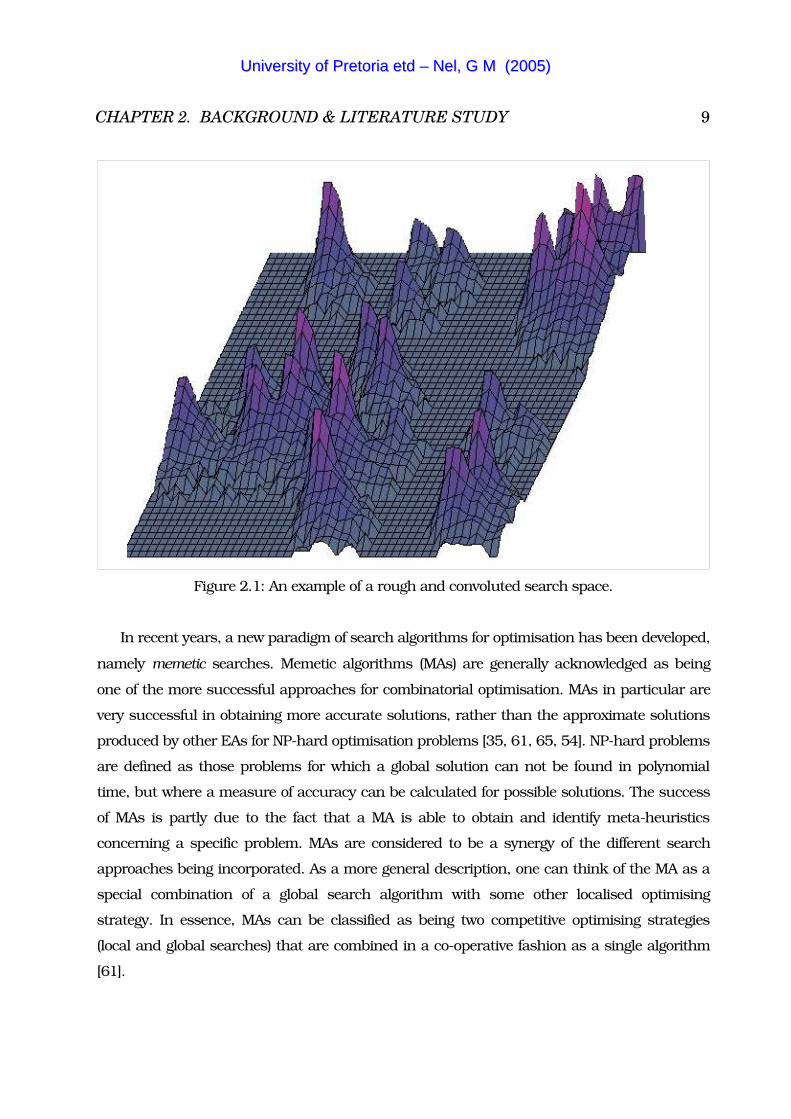
Generally, the use of a local search algorithm is discouraged when the local search space
has many optima [20], or where the search space is very rough and convoluted. Figure 2.1
below illustrates such a rough and convoluted search space. A global search algorithm, in
contrast, is more efficient in locating a solution for convoluted spaces. A global search
algorithm is faster than a local search algorithm when searching through such rough and
convoluted search spaces. However, global search is less effective in refining the solution [79,
31, 7, 49, 25].
UUnniivveerrssiittyy ooff PPrreettoorriiaa eettdd –– NNeell,, GG MM ((22000055))
CHAPTER 2. BACKGROUND & LITERATURE STUDY 9
Figure 2.1: An example of a rough and convoluted search space.
In recent years, a new paradigm of search algorithms for optimisation has been developed,
namely memetic searches. Memetic algorithms (MAs) are generally acknowledged as being
one of the more successful approaches for combinatorial optimisation. MAs in particular are
very successful in obtaining more accurate solutions, rather than the approximate solutions
produced by other EAs for NP-hard optimisation problems [35, 61, 65, 54]. NP-hard problems
are defined as those problems for which a global solution can not be found in polynomial
time, but where a measure of accuracy can be calculated for possible solutions. The success
of MAs is partly due to the fact that a MA is able to obtain and identify meta-heuristics
concerning a specific problem. MAs are considered to be a synergy of the different search
approaches being incorporated. As a more general description, one can think of the MA as a
special combination of a global search algorithm with some other localised optimising
strategy. In essence, MAs can be classified as being two competitive optimising strategies
(local and global searches) that are combined in a co-operative fashion as a single algorithm
[61].
UUnniivveerrssiittyy ooff PPrreettoorriiaa eettdd –– NNeell,, GG MM ((22000055))
CHAPTER 2. BACKGROUND & LITERATURE STUDY 10
To distinguish the MA from other optimisation methods and algorithms, and to describe
MAs better, the term meme was introduced by R. Dawkins in the last Chapter of his book
[23]. He defines memes as ideas, information, clothing fashions, ways of building bridges and
arches, catch-phrases, music and imagination. Just as genes propagate themselves in the
gene pool by leaping from body to body via sperm or ova, so do memes propagate themselves
in the meme pool by leaping from brain to brain via a process which, in the broad sense, can
be called imitation [23]. MAs use memes that are defined as a unit of information adapted
during an evolutionary process.
MAs combine global search algorithms, specifically evolutionary algorithms that make use
of evolutionary operators, with local search algorithms. The EAs can quickly determine
regions of interest in the search space, while local search algorithms refine the solution in a
localised area of the search space. A MA is therefore more efficient and effective in finding and
refining a solution than a single global search algorithm. Alternative names for MAs such as
hybrid genetic algorithms [31, 77], hybrid genetic programs [53], genetic local search
algorithms [60, 30], and knowledge-augmented genetic algorithms [11, 19], all have their
origin in the notion that a MA can be seen as an EA. This thesis, however, views MAs as
population-based evolutionary search methods for combinatorial optimisation problems. Note
that MAs use as much knowledge as possible about the combinatorial optimisation problem
to produce a solution. In some respects MAs are similar to EAs, that simulate the process of
biological evolution. However, unlike EAs that use genes, MAs use memes that are typically
adapted, and transmitted to the next generation. In [61], Moscato and Norman state that
memetic evolution can be mimicked by combining EAs with local refinement strategies such
as a local neighbourhood search, simulated annealing or any of the other local search
heuristics explained in Chapter 5. Chapter 5 also provides an in-depth theoretical discussion
regarding local search and MAs.
EAs play an important role in this thesis which holds that an EA is transformed into a
MA. Both EAs and MAs fall into a subset of the evolutionary computation (EC) paradigm.
Therefore, it is necessary to define and review that paradigm which is done in the following
Section.
UUnniivveerrssiittyy ooff PPrreettoorriiaa eettdd –– NNeell,, GG MM ((22000055))
CHAPTER 2. BACKGROUND & LITERATURE STUDY 11
2.2 Evolutionary Computation
The theory of evolution was presented by Charles Darwin in 1858 at a meeting of the Linnean
Society of London and subsequently published [21]. At the same meeting, Alfred Russel
Wallace also presented his independently developed theory of evolution and therefore shares
the credit with Darwin. In essence, the theory of evolution states that the goal of all species is
their survival, which is based on the underlying principal which is that of optimisation.
In nature evolution is driven by four key processes, namely, reproduction, mutation,
competition and natural selection [51]. Individuals in a population of a species carry the
genetic traits of the species. If the species is to survive and be more successful, then the
genetic traits have constantly to change and adapt in order that the species survives the
constantly changing environment that it occupies. Note that the environment of the species
changes due to natural causes that occur on earth.
Reproduction facilitates the change and adaptation of genetic traits of the successful
organisms in a species. Reproduction is the process whereby one or more successful parent
organisms can reproduce either by cloning or combining their genetic materials. Note that in
nature the reproduction model is very successful whereby two parents pass on their
combined genetic traits to their offspring.
Mutation, alternatively, occurs when reproduction produces new organisms as offspring,
and there is an error in the transfer of genetic material from the parent organisms to their
young. Mutation also occurs when environmental conditions force mutation of the genetic
material within an individual organism. Therefore the process of mutation can be either
harmful or beneficial to the resultant organisms. An offspring’s genetic traits (characteristics)
are, therefore, in part inherited from parents through the process of recombination, and in
part as the result of genes that are mutated in the process of reproduction.
Competition and natural selection go hand in hand because, in nature, organisms are
compelled to compete for food, living space (shelter) and the need to reproduce. Competition
for natural resources and timely reproduction usually leads to the more successful
organisms’ survival and procreation, while less successful organisms may well face
extinction. Therefore, the phrase ‘natural selection’ is used to describe the survival of the
‘fittest’. Note that the genetic traits of an unsuccessful organism are not necessarily removed
immediately, but rather they do not ‘survive’ into the next generation. If the organism is
UUnniivveerrssiittyy ooff PPrreettoorriiaa eettdd –– NNeell,, GG MM ((22000055))
CHAPTER 2. BACKGROUND & LITERATURE STUDY 12
removed immediately, the operation is then referred to as ‘culling’. In nature successful
organisms may also survive for multiple generations, a process referred to as ‘elitism’.
Evolutionary computation is inspired by Darwin’s theory of evolution, and was introduced
in the 1960s by I. Rechenberg. John Holland, in 1975, introduced genetic algorithms [36]. In
1992, genetic programming was derived from genetic algorithms by John Koza, in order to
evolve programs to perform certain tasks [46]. Today, the different evolutionary algorithms
that were developed in the EC paradigm include genetic algorithms (GA) [9, 59, 60, 36],
genetic programming (GP) [13, 69, 46, 24, 50], evolutionary programming (EP) [6, 7, 37],
evolutionary strategies (ES) [5, 45], co-evolution and cultural evolution (CE) [25].
As a principle, EC algorithms emulate nature by implementing the four key evolutionary
processes given above as operators which affect a population of individuals. The
mathematically encoded solution to a problem is known as the genotype of an individual in
an EC algorithm. Therefore, a population of individuals in the problem space encodes a set of
possible solutions. In nature the equivalent of a mathematical representation of the individual
are the genetic traits (genes) of a successful organism. Therefore, the genotype carries genetic
information encoded in an individual. The set of related properties that a population of
individuals may exhibit in a specific environment is known as the phenotype of a population.
In other words, the phenotype is the behaviour exhibited by the genotype of a population in a
certain environment. Interactions between, and dependencies of the phenotype and genotype
of a population can be quite complex. Note that in natural evolution, the mapping between
phenotype and genotype is a non-linear function (not one-to-one mapping), and represents
interaction between genes and the environment. Unexpected variations in phenotypes can be
caused by a random change in a fragment of information in the genotype, a process known as
pleiotropy [51]. A specific phenotype trait is produced by the interaction of several pieces of
information in the genotype and is known as polygeny [51]. Therefore, a specific phenotype
trait can be changed only if all relevant pieces of genotypic information that individuals
possess are changed.
Evolutionary computation is used not only to solve optimisation problems, but also has
been found to be useful in a variety of applications. These relate to problems that overlap
somewhat, but all were previously thought of as being computationally intractable.
Application categories in which EC has successfully been used [26, 46, 55, 18, 76, 4, 38]
include:
UUnniivveerrssiittyy ooff PPrreettoorriiaa eettdd –– NNeell,, GG MM ((22000055))
CHAPTER 2. BACKGROUND & LITERATURE STUDY 13
� simulation,
� classification and identification,
� design and planning,
� process control systems, and
� image feature extraction.
The participation of EC algorithms in the referred categories vary depending on the
application and the particular EC algorithm used. EC have proved to be very successful in
providing solutions for the problems of the above mentioned categories, in spite of such
problems being both complex and time consuming to solve. However, one of the drawbacks of
many EC methods, specifically the global search variety, is that even though they may be
relatively efficient in finding a solution, it seldom has high accuracy. Therefore, most global
search methods do not have a good ‘exploiting capability’. The inaccuracy of the global
solution found is an inherent drawback specifically built into most global search methods. It
is required that the implemented global search algorithm must not return solutions at specific
local optimum points before the full search space has been explored.
The following Section reviews broadly and discusses the strategies and operations shared
by all EAs. Another important aspect regarding an EA is the representation of the genotype of
individuals in its population. The representation of the genotype is reviewed in detail in the
final Section below regarding rule extraction, where it is appropriately discussed since its
influence is paramount on the rule extraction process.
2.3 Evolutionary Algorithms
This Section provides a review of EAs, their operations, strategies, and general architecture.
First, the benefits of using EAs are listed. Then the general architecture for a classical EA is
discussed, followed by the algorithm framework. The latter is used to review the initialisation
of the population, the EA operators and the issues relating to EAs. Several strategies that
were devised for some of the operators are also discussed. Finally, the issues that all EAs face
are listed and discussed.
UUnniivveerrssiittyy ooff PPrreettoorriiaa eettdd –– NNeell,, GG MM ((22000055))

CHAPTER 2. BACKGROUND & LITERATURE STUDY 14
2.3.1 Benefits and General Architecture
The benefits of using EAs include the following:
� The evolution concept is easy both to understand and to represent in an algorithm.
� The implementation of an EA can be kept separate from another application that utilises it,
as it is modular.
� Multiple solutions can be produced for a multi-objective problem, and multiple fitness
functions can be used simultaneously [19, 5, 18].
� The EA algorithm can be distributed easily over several processors, because some of the
operations in an EA are inherently parallel.
� Some of the previous or alternate solutions can easily be exploited by using EA parameter
settings.
� As knowledge about a problem domain is gained, many ways become apparent that can be
used to manipulate the speed and accuracy of an EA-based application.
� ‘Noisy’ data are handled while reasonable solutions can still be delivered by EAs.
� An EA always produces an answer.
� The answers become more accurate with time.
The different benefits of EAs will become even more apparent over the following
paragraphs as the architecture, operators and different strategies are discussed. All EAs have
the same general architecture:
1. Initialise the population.
2. While not converged,
(a) Evaluate the fitness of each individual,
(b) Perform evolutionary operations such as reproduction and mutation,
(c) Select the new population.
3. Return the best individual as the solution found.
The different EA paradigms that were mentioned in the previous Section, e.g. GA, GP, EP, ES
and CE, can be distinguished by the population size relationship between parent and
offspring populations, representation of the individuals, as well as the operator strategies that
are used. Note that because GP was derived from GA, GP is treated as a specialised GA with a
UUnniivveerrssiittyy ooff PPrreettoorriiaa eettdd –– NNeell,, GG MM ((22000055))

CHAPTER 2. BACKGROUND & LITERATURE STUDY 15
different representation for the individuals in its population. This thesis concentrates on a
specific implementation of a GP, and for that reason, the evolutionary procedure outlined
above is discussed with the GP paradigm in mind. In order to define properly and elaborate
on the evolutionary process, some mathematical notation should be explained.
The search space SP was defined in Section 2.1.1 as being the set of all possible solutions
to problem P. Assume first that a population of � individuals at time t is given by P(t) � (x1(t),
x2(t), ..., x�(t)). Every x� � SP represents a possible solution for problem P in the search space.
Every individual solution x� has a relative measure of accuracy in solving P. Let the fitness
function, f(x�), which is also known as the evaluation function, decode the genotype
representation of x� and assigns it a fitness measure. Therefore the fitness of the whole
population in SP at time t can be expressed as F(t) � (f(x1(t)), f(x2(t)), ..., f(x�(t))). Generally,
solutions are normalized and compared with one another in how well each possible solution
solves the particular problem at hand. Normalisation of the solutions will be explained in
detail when the population selection process is discussed in Section 2.3.7.
The objective function is defined next in order to compare the solutions that are produced.
The objective function is described as both the implicit and user-specified constraints under
which solutions are optimised. The fitness function, which is a function applied to the
chromosomes of an individual, is used to determine the fitness of an individual, and depends
on the objective function. The fitness function can also depend on the specific representation
of the individual used by the specific algorithm [30]. Note that it is only the fitness function
which links the EA and the problem it is solving. No other process in the EA links it with the
problem being solved. The reproductive operators use the fitness function to compare
individuals with one another and are therefore dependent on it. For example, the selection
operator uses the fitness function to determine which individuals will ‘survive’ to the next
generation. It is also important to note that the representation of the genotype will influence
the fitness function, since the fitness function decodes the genotype representation of x� (an
individual solution) and assigns to it a fitness measure. Hence, the choice of fitness function
along with the genotype representation is very important when implementing an EA.
The pseudo-algorithm (framework) representing the classical EA in more detail is provided
by, and adapted from several authors [26, 57, 65, 46, 30, 3, 4, 56], as given in Figure 2.2. The
population at time t, P(t), and the fitness of the population at time t, F(t), have already been
UUnniivveerrssiittyy ooff PPrreettoorriiaa eettdd –– NNeell,, GG MM ((22000055))
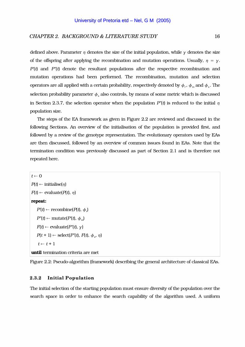
CHAPTER 2. BACKGROUND & LITERATURE STUDY 16
defined above. Parameter � denotes the size of the initial population, while denotes the size
of the offspring after applying the recombination and mutation operations. Usually, � � .
P'(t) and P''(t) denote the resultant populations after the respective recombination and
mutation operations had been performed. The recombination, mutation and selection
operators are all applied with a certain probability, respectively denoted by r , m and s . The
selection probability parameter s also controls, by means of some metric which is discussed
in Section 2.3.7, the selection operator when the population P''(t) is reduced to the initial �
population size.
The steps of the EA framework as given in Figure 2.2 are reviewed and discussed in the
following Sections. An overview of the initialisation of the population is provided first, and
followed by a review of the genotype representation. The evolutionary operators used by EAs
are then discussed, followed by an overview of common issues found in EAs. Note that the
termination condition was previously discussed as part of Section 2.1 and is therefore not
repeated here.
t � 0
P(t) � initialise(�)
F(t) � evaluate(P(t), �)
repeat:
P'(t) � recombine(P(t), r)
P''(t) � mutate(P'(t), m)
F(t) � evaluate(P''(t), )
P(t + 1) � select(P''(t), F(t), s, �)
t � t + 1
until termination criteria are met
Figure 2.2: Pseudo-algorithm (framework) describing the general architecture of classical EAs.
2.3.2 Initial Population
The initial selection of the starting population must ensure diversity of the population over the
search space in order to enhance the search capability of the algorithm used. A uniform
UUnniivveerrssiittyy ooff PPrreettoorriiaa eettdd –– NNeell,, GG MM ((22000055))
CHAPTER 2. BACKGROUND & LITERATURE STUDY 17
random selection is the preferred method whereby the initial population is selected, since the
probability is better that the spread in terms of fitness values of individuals are more
uniformly distributed. A diverse selection will ensure that the fitness of the initial generation is
significantly lower than the fitness of the optimal solution. The task of the evolutionary
process is, therefore, to improve the fitness of the initially stochastically selection of
individuals.
2.3.3 Representation of the Genotype
The representation of the genotype is important because the strategies and evolutionary
operators of an EA depend greatly on representation of the individuals. Traditionally, EAs
such as GAs implement the genotype representation as a binary encoding, in other words an
encoded bit string [26, 77, 59, 19]. The main problem with the binary encoding scheme is
that there is a loss in accuracy when a mapping occurs between a binary string of limited
length, and real-valued data that the binary string represents. This loss of accuracy occurs
since binary encoding functions are complex, and if finer granularity is required in the
mapping, then a more complex encoding scheme (longer binary string length) is required. If a
binary string of variable length is used, then the evolutionary operators and strategies
engaged need to be altered to accommodate the encoding.
The binary encoding scheme is not the only representation scheme used. Some GAs use
the real values in data directly and indirectly in their genotype representations [27, 41].
Another encoding scheme also employed is the permutation encoding scheme as used in [22],
for example, the travelling salesman problem [61]. Tree-based representations are used in the
GP paradigm [68, 13, 69, 46, 24, 50, 53]. The tree-based representations are discussed in
detail in Section 3.1.2.
2.3.4 Evolutionary Operators
The evolutionary operators, namely recombination (also known as crossover), mutation and
selection which includes elitism, implement a pseudo-random walk through the search
space. It is a pseudo-random walk because the recombination, selection and mutation
operators are applied with a certain probability, which makes the operators non-
deterministic. Note that the pseudo-random walk is directed, because recombination,
UUnniivveerrssiittyy ooff PPrreettoorriiaa eettdd –– NNeell,, GG MM ((22000055))

CHAPTER 2. BACKGROUND & LITERATURE STUDY 18
mutation and selection try to maximize the quality of the possible solutions. The evolutionary
operators that were mentioned are provided and discussed in the following Sections.
2.3.5 Recombination
The goal of the recombination operation is to enable the EA to look for solutions near existing
solutions. Recombination achieves this goal by combining (pairing) of genetic material of two
or more randomly chosen parent individuals to produce offspring individuals. The
recombination of two or more individuals involves the exchange of certain randomly chosen
parts of parents to create a new individual, which is added to the original population. The
parts that are randomly chosen are the points in the parent individuals where the exchange
will occur, and are referred to as the swap points. The recombination probability parameter,
r , is often applied with a high probability to ensure that crossover occurs frequently. The
latter is so in order to induce convergence in the EA. Several types of crossover strategies have
been devised for EAs [26, 46, 30]:
� One-point crossover,
� Two-point crossover,
� Uniform crossover, and
� Arithmetic crossover.
The choice of crossover strategy depends on the specific EA algorithm that is implemented, as
well as the representation of individuals of the EA. Note that crossover for decision trees is
reviewed in Section 3.1.2. As an example, to illustrate the different crossover strategies for
EAs, assume that a GA with a bit string representation is used.
With one-point crossover, a single swap point in the bit string is selected, and all the bits
after the swap point are swapped out with the respective bits of the associated parent. Figure
2.3 illustrates one-point crossover.
Figure 2.3: One-point crossover with parents in (a) and offspring in (b).
10110|010 1011010001001|100 01001010
(a) (b)
UUnniivveerrssiittyy ooff PPrreettoorriiaa eettdd –– NNeell,, GG MM ((22000055))
CHAPTER 2. BACKGROUND & LITERATURE STUDY 19
With two-point crossover two swap points are selected randomly, and the bits between the
swap points are exchanged. Two-point crossover will, on average, select a smaller segment to
swap than one-point crossover. Therefore, two-point crossover is more conservative than one-
point crossover when changing the individuals.
Uniform crossover works completely differently in that the bits that are swapped are
selected at random by sampling from a uniform distribution. The selection of bits occurs with
a certain probability, which can also be specified to the algorithm as an additional input
parameter. Once a bit which is to be swapped has been selected, the corresponding bits in the
parents are swapped out.
Arithmetic crossover is specifically used in EAs where the representation of the individual
is real-valued. Assume two parent individuals, xk(t) and xl(t), exist at time t. Let d be a
uniform random variate in the range (0, 1), therefore d � U(0,1). Parents xk(t 1)and xl(t 1)
are mutated at time t 1 with the following respective functions:
xk �t�1���d � xk �t ���1.0�d � xl �t �
and
xl �t�1���d � xl �t ���1.0�d � xk �t �
Note that more than two parents can be chosen for recombination as in, for example,
differential evolution where more than two parent individuals are used when performing
recombination [74]. As this thesis uses a specific GP algorithm, the crossover strategies
specific to GP are discussed in Section 3.1.2.
2.3.6 Mutation
Mutation is used to randomly change the genetic material of an individual. The purpose of
mutation is to introduce new genetic material into the population, thereby increasing the
diversity of the population. Therefore, the mutation operation enables the EA to look at
completely new areas of the search space. Hence, a larger part of the search space is
searched. The mutation probability parameter, m , is usually set high, but decreases as the
fitness of the individuals in the EA improves. In fact it is recommended that m � F(t),
UUnniivveerrssiittyy ooff PPrreettoorriiaa eettdd –– NNeell,, GG MM ((22000055))
CHAPTER 2. BACKGROUND & LITERATURE STUDY 20
because initially the EA needs to explore more unexplored regions of the search space for
possible solutions. As the EA evolves solutions over the generations, and the population
fitness improves, the probability to mutate must be reduced in order to reduce the chance
that highly fit individuals are mutated. Several mutation strategies specific to GP have been
devised [13, 15]. The GP specific mutation strategies are explained in Section 3.1.2. Other
known mutation strategies include bit flip mutation [60, 18], and promote and demote
mutation [48].
2.3.7 Selection
The function of the selection operator is to reduce the size of population P(t + 1) back to the
original number of individuals, �, after the recombination and mutation operators have been
applied. Remember that the recombination and mutation operators add offspring to the
original population. However, to simulate Darwin’s evolution theory effectively, every new
generation must be equal to the initial generation in population size. Therefore, individuals
must be selected to be removed from the � + set of individuals. Note however that the
selection operation is directed, meaning that preference is given to certain individuals with
higher fitness values, rather than individuals with lower fitness values. In fact, a selection
strategy, namely elitism, has been devised that ensures that a certain percentage of the
population, say the top 20% in terms of their fitness value, survives to the next generation by
copying directly that subpopulation to P(t + 1). Note that selection strategies in Section 3.1.2
are used to select individuals from the population after recombination, mutation, elitism and
selection of the new population operations have been performed. The value of the fitness
function f(x�) for individual x� is compared with the fitness values of other individuals in the
population when deciding whether an individual is selected or not. Therefore, the fitness
function is the selection criterion used during the selection process. Several selection
strategies have been devised in order to allow for a higher probability for selecting individuals
with higher (or lower) fitness values [10, 15, 26, 46, 68, 76], namely:
� Roulette Wheel Selection,
� Rank Selection,
� Steady State Selection, and
� Tournament Selection.
UUnniivveerrssiittyy ooff PPrreettoorriiaa eettdd –– NNeell,, GG MM ((22000055))
CHAPTER 2. BACKGROUND & LITERATURE STUDY 21
The selection operators listed above are discussed in the following paragraphs.
Roulette Wheel Selection
With roulette wheel selection, each individual is assigned a slice of the wheel in proportion to
the fitness value of the individual. Therefore, the fitter an individual is, the larger the slice of
the wheel. The wheel is simulated by normalising the fitness values of the population of
individuals. Normalisation of fitness values of the individuals implies that all the fitness
values must add up to 1. The roulette wheel strategy is best explained by the following
example. Assume there is a set of four individuals (x1, x2, x3, x4) in the population of possible
solutions. Assume that the normalized fitness of the set is (0.1, 0.2, 0.3, 0.4), which add up
to1. For individual x1 a range from 0 (exclusive) to 0.1 (inclusive) is assigned, i.e. x1 � (0.0,
0.1]. For individual x2 a range from 0.1 (exclusive) to 0.3 (inclusive) is assigned, i.e. x2 � (0.1,
0.3]. The high-end normalized range value of x2 is calculated by adding the normalized values
of x1 and x2. The range values of x3 and x4 are determined and assigned in similar fashion,
and is therefore x3 � (0.3, 0.6], x4 � (0.6, 1.0]. Clearly x4 has the largest proportion of the
range (0.0, 1.0], which is the equivalent of the roulette wheel, while x1 has the smallest
proportion. Hence, x4 has a better probability of being selected than x1 . A random number is
then generated from a uniform distribution U(0.0, 1.0]. Assume the random number is 0.5,
then the selected individual is x3 , because 0.5 fall within the range represented by x3 . As a
result of performing roulette selection, the individual with the best fitness value has a better
chance of being selected.
Rank Selection
Rank selection is performed by first ranking the population of individuals according to the
fitness. Using the example in the roulette wheel strategy, x1, x2, x3, and x4 would be ranked
(4, 3, 2, 1). A random selection from the set {1, 2, 3, 4} is made to choose the individual. Note
that rank selection is based on the ranking of the individuals, and not their fitness value.
Hence, the rank selection method focusses rather on the rank while ignoring absolute fitness
differences between the individuals. As a result of performing rank selection, highly fit
individuals cannot dominate, such as when a fitness-based selection is performed.
UUnniivveerrssiittyy ooff PPrreettoorriiaa eettdd –– NNeell,, GG MM ((22000055))
CHAPTER 2. BACKGROUND & LITERATURE STUDY 22
Steady State Selection
With steady state selection a few individuals with high fitness values in every generation are
selected for creating new offspring individuals. The new offspring individuals replace the
parent individuals only if the offspring is more fit than the parents. The whole population is
then selected for the new generation.
Tournament Selection
Several variations of the tournament selection strategy exist [68, 76, 10]. Only two popular
variations are provided here. The first is to divide the population into groups by adding at
random an individual to a group. After the population is divided into several groups, select the
best individuals in terms of fitness values from each group. Note that each individual cannot
appear in more than one group. Thereby, individuals within the groups compete with one
another.
The second variation uses a given value n to compare n individuals with one another.
Randomly select n individuals as the subpopulation to be used. Individual xn of the sub-
population of n individuals is compared with the rest of those in the sub-population. The
individual xn scores a point if it has a higher fitness value than another individual in the sub-
population. Hence, the individuals in the sub-population can be ranked according to the
points they score when compared to other members in the sub-population. If n is set to a low
value, the ranking of individual xn is not necessarily unique, since it then depends on other
individuals in the sub-population to which it was compared. Hence, the selection pressure is
low, and therefore approaches random choice. If n = , then the sub-population will be equal
in size to the population, and an unique ranking is possible for each individual, as is the case
with the rank selection strategy. The result of choosing a small value for n is that a truly
random selection of individuals is achieved, while a larger value for n will force a selection
according to rank.
2.3.8 Issues in EA
Some common issues that require careful consideration when selecting a specific EA
implementation exist in all EAs. Often the hardest and most important choice in producing a
UUnniivveerrssiittyy ooff PPrreettoorriiaa eettdd –– NNeell,, GG MM ((22000055))
CHAPTER 2. BACKGROUND & LITERATURE STUDY 23
good solution is the fitness function that will be used [46, 4, 56, 12]. However, the
representation of the genotype of the individuals in the population usually influences the
choice of fitness function, as well as strategies implemented by the evolutionary operators.
Careful consideration must be given to the input parameters, which include the population
size and operator probability parameters which were discussed. It is important to consider the
population size because if the number of individuals is too few, then a proper exploration of
the search space is unlikely. A large population size can conceivably cause problems if the
hardware that the EA is executed on does not have enough resources. Furthermore, a large
population would induce more evolutionary operations which increase computational
complexity unnecessarily, while a smaller population can find a solution of equal accuracy
with less associated computational difficulty. Unfortunately, the systems that EAs run on are
all limited in resources in some way or the other. Those limitations often include the
processing power and memory capabilities of the system.
The importance of the selection of a correct representation for the encoding scheme was
discussed in detail in Sections 2.3.1 and 2.3.3 above. Another very important consideration
involves the recombination rate and mutation rate. The recombination rate controls the rate
that the algorithm will converge. If the algorithm converges too fast, then the probability that
the search space is not properly explored increases. If the recombination rate is selected at a
low level, the algorithm will require more generations before converging to a solution of
sufficient accuracy. The mutation rate controls the pace with which new regions of the search
space is explored. If the mutation rate is selected too high, the algorithm may not converge at
all to a solution. If the mutation rate is selected low, very few new possible solutions are
introduced. Hence, the search capability of the algorithm is reduced.
The selection strategy and the policy for the deletion of individuals from the population are
further issues that are partly decided by the specific EA implementation in use. The choice of
termination criteria that is commonly used by most of the EAs was discussed above as part of
Section 2.1.
Another issue that EAs have to consider is that the solutions produced must not over-fit
the problem data. With over-fitting it is meant that the solutions do not generalise the data
well. Over-fitting of the data is discussed in more detail in the following Section. The choice of
the specific EA implementation is also influenced, but not determined, by the ease with which
the problem data are mapped to the genotype representation of the individuals of the specific
UUnniivveerrssiittyy ooff PPrreettoorriiaa eettdd –– NNeell,, GG MM ((22000055))
CHAPTER 2. BACKGROUND & LITERATURE STUDY 24
implementation. If the mapping is incorrect, the solutions produced will be sub-optimal and
less useful in terms of solving the problem.
The representation of the individuals is especially important when rules are extracted from
solutions produced by EAs. Hence, representation of the individuals is discussed in detail in
the next Section. There also are reviewed concepts associated with the process of knowledge
discovery.
2.4 Rule Extraction
In order to understand clearly the process of rule extraction, a motivation for performing it is
required. Such a motivation for performing knowledge discovery is given in the following
Section. Knowledge discovery is then described in detail and the subsequent process of
performing rule extraction is given. Finally, an overview is then provided of current methods
by which to perform knowledge discovery.
2.4.1 Motivation for Knowledge Discovery
Knowledge discovery has become important in recent times because most corporations have
acquired and are storing vast quantities of data that is subsequently analysed in order to
remain competitive. Computation systems and methods for analysing databases have
improved considerably in recent times. The direct result is a reduction in the cost associated
with automated knowledge discovery. For example, a company can be more competitive by
identifying trends and constraints within the market in which it competes by storing market-
associated data, and subsequently analysing it. However, the stored data has to be analysed
and classified within a reasonable time frame in order to be useful in a competitive
environment. A further requirement is that the trends and constraints of the market must be
determined with sufficient accuracy in order to be useful. The costs involved in the production
of a product or delivery of a service can be part of the constraints. The constraints associated
with products and services are not static. They change over time. Consider the mobile phone
market which is constantly changing with the introduction of new technologies (trends) and
new mobile phone models, with the retirement of older types. The technology used in a mobile
phone, and the materials used to construct it have an ever changing cost component. Mobile
phone manufactures can use information regarding the costs involved when producing their
UUnniivveerrssiittyy ooff PPrreettoorriiaa eettdd –– NNeell,, GG MM ((22000055))

CHAPTER 2. BACKGROUND & LITERATURE STUDY 25
products. If the cost is known, then competitive pricing of the item can be determined
optimally. Therefore, rules are required that describe the trends and constraints (such as
costs) associated with a product or service. The rules can be used to determine pricing of
products and services, and can give important guidance when strategic business decisions
are made.
A set of rules is the preferred format of the output when solving a classification problem,
because humans can understand and interpret rules. For example, the rule ‘IF cost to
produce mobile phone A is high AND profit margin is low AND demand for mobile phone A is
low THEN stop production of mobile phone A’, is clear and unambiguous. The example rule
helps to determine when it is no longer profitable to produce mobile phone A, as when
combination of the production cost, and the demand for mobile phone A is at a certain
threshold. Hence, a rule concerning the constraints and trends associated with a concept is
more useful to humans than the raw data in the database regarding it.
The constraints and trends associated with a product or service, in other words the
dataset that describes the product or service, are dynamic. Therefore, the rules describing the
data must also be dynamic. Traditionally, such rules are extracted by humans who perform
the analysis and classification of the data describing products or services. However, due to the
sheer volume of information available and the number of variables to take into account, the
task of analysing and classifying data has become complex and time-consuming at best.
Once a set of rules has been determined that sufficiently describes the dataset, it is very
difficult to allow for any subsequent addition of further relevant attributes without affecting
any or all of the existing rules. Such an introduction of additional relevant attributes would
increase the complexity of the problem, and could render existing classification rules obsolete.
To repeat the whole analysis phase can be time-consuming, while placing a considerable
strain on existing resources. The set of rules can also be more difficult to extract from the
dataset if more attributes are added. Therefore, the competitiveness and productivity of any
company or person may be seriously impeded.
Professionals such as mathematicians, physicists, chemists, engineers, medics,
economists and many others can also gain from using knowledge that describes data (meta-
data) that they work with. For example, a chemical plant can be designed optimally if certain
constraints such as running costs, environmental pollution and the required maintenance
intervals are known in advance during the design phase.
UUnniivveerrssiittyy ooff PPrreettoorriiaa eettdd –– NNeell,, GG MM ((22000055))
CHAPTER 2. BACKGROUND & LITERATURE STUDY 26
Clearly, the process of automated knowledge discovery compared to a traditional type of
analysis done by humans has some advantages, namely:
� shorter time to solution (classification) period,
� more adjustable and dynamic to parameter and attribute changes,
� improved accuracy in solutions (classifications),
� less costly and more consistent than human classifiers,
� no or very little expertise required to perform analysis, and
� may be used for multiple problems.
The next Section defines and describes the process of knowledge discovery.
2.4.2 Knowledge Discovery
Knowledge discovery can be defined as the non-trivial process of identifying and extracting
useful, valid, novel and understandable knowledge from data [68, 66]. The process of
knowledge discovery may be described as the accumulation of knowledge about data, in other
words, meta-data, and the subsequent analysis of that meta-data in order to extract rules
that describe with sufficient accuracy the behaviour of the data. The extracted rules can then
be applied in identifying concepts in the data with the same syntax and semantics within the
same context. The general form of a rule (also known as a ‘conditional expression’) is
exemplified as:
IF antecedent THEN consequence (2.1)
Two types of rules can be defined, namely characterisation rules and discriminant rules. With
characterisation rules, the objective is to find rules that describe the properties of a concept.
Characterisation rules have the form:
IF concept THEN characteristic (2.2)
With discriminant rules, the objective is to find rules that allow the selection (discrimination)
of the objects (data records), belonging to a given concept (class), from the rest of the objects
(data records or classes). Discriminant rules have the form:
UUnniivveerrssiittyy ooff PPrreettoorriiaa eettdd –– NNeell,, GG MM ((22000055))

CHAPTER 2. BACKGROUND & LITERATURE STUDY 27
IF characteristic THEN concept (2.3)
Note that the inverse implication of the characteristic rule is not a discriminant rule. An
extracted rule from a dataset that performs a classification of instances belonging to a class in
the set is sometimes referred to as a classifier. For example, the following unordered rule set
can be used to divide and group data instances in a two-dimensional (x and y attributes)
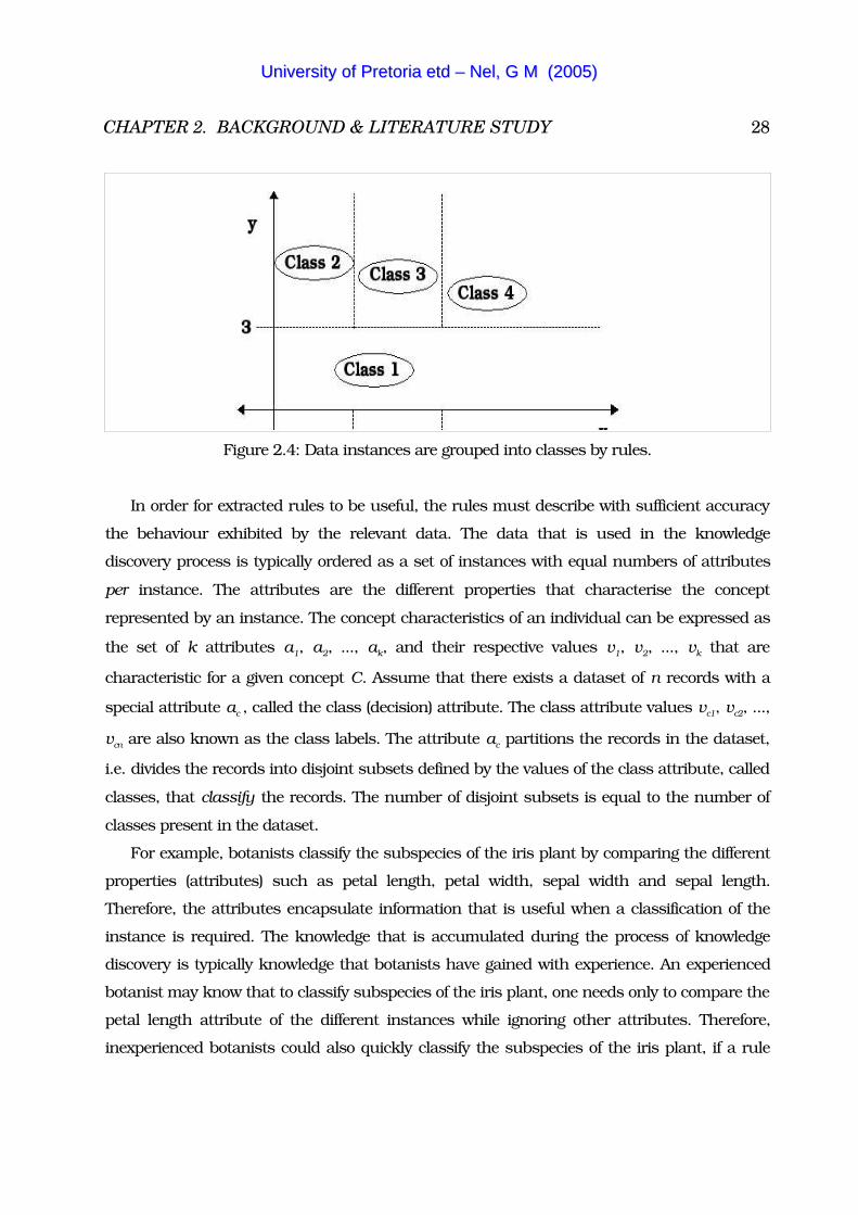
problem space. The unordered rule set is visually represented by Figure 2.4:
IF y � 3 THEN class 1;
IF y � 3 AND x � 3 THEN class 2;
IF y � 3 AND x � 3 AND x � 4 THEN class 3;
IF y � 3 AND x � 4 THEN class 4;
If the rules are read in a certain order, then the ordered rules can be further simplified as
follows:
1. IF y � 3 THEN class 1;
2. IF x � 3 THEN class 2;
3. IF x � 3 AND x � 4 THEN class 3
(which can be further simplified to: IF x � 4 THEN class 3 );
4. IF x � 4 THEN class 4;
Note that each condition in the rules above is a boundary as illustrated in Figure 2.4. The
data instances are divided (split) into the illustrated classes if they fall within the class regions
formed by the boundaries as illustrated.
UUnniivveerrssiittyy ooff PPrreettoorriiaa eettdd –– NNeell,, GG MM ((22000055))
CHAPTER 2. BACKGROUND & LITERATURE STUDY 28
Figure 2.4: Data instances are grouped into classes by rules.
In order for extracted rules to be useful, the rules must describe with sufficient accuracy
the behaviour exhibited by the relevant data. The data that is used in the knowledge
discovery process is typically ordered as a set of instances with equal numbers of attributes
per instance. The attributes are the different properties that characterise the concept
represented by an instance. The concept characteristics of an individual can be expressed as
the set of k attributes a1, a2, ..., ak, and their respective values v1, v2, ..., vk that are
characteristic for a given concept C. Assume that there exists a dataset of n records with a
special attribute ac , called the class (decision) attribute. The class attribute values vc1, vc2, ...,
vcn are also known as the class labels. The attribute ac partitions the records in the dataset,
i.e. divides the records into disjoint subsets defined by the values of the class attribute, called
classes, that classify the records. The number of disjoint subsets is equal to the number of
classes present in the dataset.
For example, botanists classify the subspecies of the iris plant by comparing the different
properties (attributes) such as petal length, petal width, sepal width and sepal length.
Therefore, the attributes encapsulate information that is useful when a classification of the
instance is required. The knowledge that is accumulated during the process of knowledge
discovery is typically knowledge that botanists have gained with experience. An experienced
botanist may know that to classify subspecies of the iris plant, one needs only to compare the
petal length attribute of the different instances while ignoring other attributes. Therefore,
inexperienced botanists could also quickly classify the subspecies of the iris plant, if a rule
UUnniivveerrssiittyy ooff PPrreettoorriiaa eettdd –– NNeell,, GG MM ((22000055))
CHAPTER 2. BACKGROUND & LITERATURE STUDY 29
regarding the iris petal length attribute existed. Therefore, knowledge about data can be very
useful.
A common problem that all classifiers encounter is linked to the quality associated with
the data on which knowledge discovery is performed. In a perfect world, the data that is used
in the knowledge discovery process is flawless. However, data in the real world has two
common defects namely, ‘outlier’ data instances and so called ‘white noise’ data. An outlier
data instance has a class attribute value that incorrectly classifies the concept that the rest of
the attributes of the instance describe. White noise data, also known as Gaussian noise, is
defined as data with a small variance and zero mean. Therefore, it is data that has a close
proximity to the true data point, and is incorrect with only a small difference in a few
attributes. In other words, for a white noise data instance the class attribute value is correct,
but some of the instance attribute values do not describe correctly, to some degree, the
concept given by the class attribute value. White noise data may also contain incomplete data
attribute values that do not influence the classification of the data instances to which they
belong. A good EC algorithm that is robust is not significantly influenced when producing
solutions while using data that contains both outlier data instances, and white noise data. On
the other hand, a human may have difficulty discerning and disregarding the outlier and the
white noise data instances.
2.4.3 Rule Extraction
The process of rule extraction (RE) can be thought of as a transformation of nominal,
continuous or discrete knowledge from a dataset into useful symbolic propositional logical
rules that describe with sufficient accuracy the knowledge embedded in datasets [68, 24]. The
rules (knowledge) extracted during the knowledge discovery process need to adhere to the
following criteria:
� Rules must be comprehensible.
� Rules must be short, simple, crisp and clear.
� Rules must be accurate in describing the data from which they were extracted.
� Avoid duplication of rules.
� Knowledge encapsulated in rules must be useful.
Data mining is the process whereby useful and valid rules (knowledge) are extracted from
UUnniivveerrssiittyy ooff PPrreettoorriiaa eettdd –– NNeell,, GG MM ((22000055))

CHAPTER 2. BACKGROUND & LITERATURE STUDY 30
large databases by means of a classification method [68, 24, 50]. The process of data mining
is as follows.
1. Pre-process data in the database that is to be used with a rule extraction method. For
example, the raw data in the database may not be in a format that is useful to the
algorithm used. Depending on the algorithm used, missing attribute values may need to be
replaced with a value that is the average value calculated for the specific attribute.
2. An EA needs as input data some knowledge about the attributes of the given dataset, such
as which attributes are continuous, discrete or nominal.
3. Create training and validation (test) datasets if a supervised learning strategy is used.
4. Use an algorithm or method to find a solution that describes the data in the database with
sufficient accuracy.
5. A Post-process procedure which involves extracting useful rules from the solution found.
The post-processing procedure is the means whereby useful rules are extracted and
presented to a human for interpretation and use. Since this thesis concentrates on a
supervised learning method for rule extraction, the focus will be supervised learning. To build
the rule set to classify a dataset, a local, or a global, or a hybrid of a local and a global
algorithm is used in two phases: training and validation (testing). In Section 2.1, the process
of supervised learning and the use of training and testing datasets were introduced. To
elaborate on the supervised learning process, a further example is now provided.
Assume that there exists a database with a dataset of instances of which a subset of the
instances is already classified, therefore the classifications are already known. The disjoint
subset consists of the unknown data instances that have to be classified. Therefore, rules
(classifiers) are required to classify the unknown instances. The subset of known classified
instances is used to build the classifiers, which is further divided into disjoint sets of training
and test datasets. The training dataset is used to determine the class boundaries. Hence, the
class attribute values are required for the training set. The test dataset has the same format
as the training dataset, but does not require the class attribute values. The latter are used
with the test set to determine whether the predictions of the classifier coincide with the target
prediction. Therefore, the test dataset is used to determine the predictive accuracy of the set of
rules. This accuracy is expressed as a percentage of the correctly classified instances in the
test dataset. The process of selecting the test and training datasets can be quite complex and
UUnniivveerrssiittyy ooff PPrreettoorriiaa eettdd –– NNeell,, GG MM ((22000055))
CHAPTER 2. BACKGROUND & LITERATURE STUDY 31
is outside the scope of this thesis. The predictive accuracy is used as a measure of fitness to
determine how accurate the rules are that were built during the training phase. The algorithm
used will terminate when the predictive accuracy reaches an acceptable level, or when a
predetermined time has elapsed.
Therefore, classifiers (extracted rules) in the data mining process are the final product of a
classification algorithm and a dataset. Examples of classification algorithms include [6, 25,
68, 53, 18, 64, 56, 38, 43, 78, 72, 71, 14, 33, 34, 63]:
� Neural Networks,
� Bayesian Networks,
� Rough Sets,
� Decision Trees (ID3, C4.5), and
� Evolutionary Algorithms.
Other known methods for performing classification include case-based reasoning, fuzzy
set approaches, and the k-nearest neighbour classification method [25, 43, 78, 63, 47, 70].
The latter method is performed whereby data instances are represented as points in
Euclidean space. The distance to a neighbouring instance is measured as a Euclidean
distance, hence groups of neighbours are commonly classified. A short taxonomy of the
different available classification algorithms used for performing rule extraction is now
provided.
Neural Networks
The objective of a neural network (NN) is to simulate operations of the human brain [38, 43,
78, 72, 71]. Three types of nodes, namely, input, hidden and output nodes, are used with
interconnecting weights between them. Note that input nodes situated in the first level
exclusively connect with interconnecting weights to hidden nodes in the next level. Hidden
nodes connect either to more hidden nodes in the next level or to the output nodes in the final
level. Note that hidden nodes can not connect to hidden nodes in the same or previous levels,
except when working with recurrent- or Hopfield NNs,. When a node is identified as being
important, the interconnecting weight is changed (increased or decreased depending on how
the identified node is increased), which means that the node will have more influence that
other nodes at the same level. The NN ‘learns’ by adjusting weights between the nodes.
UUnniivveerrssiittyy ooff PPrreettoorriiaa eettdd –– NNeell,, GG MM ((22000055))
CHAPTER 2. BACKGROUND & LITERATURE STUDY 32
Hence, the objective of a NN is to obtain a set of interconnecting weights and nodes through
training that classifies almost all the data into the correct classes in the training data.
Some of the advantages of NNs include a generally high predictive accuracy. A NN has
high robustness when data contains errors such as ‘white noise’. The output of a NN is
always one or more continuous value(s), except when an additional function is used to map
the continuous values to discrete values. A NN that was trained beforehand is quick when
performing a classification or prediction.
Some of the disadvantages of NNs are that a NN trains notoriously slowly when the NN are
used for different problems. A NN is not robust when the data contains errors such as outlier
instances. Only when a ‘robust estimator’ is used with a NN, can data with outlier instances
effectively be classified. Complex NNs (those with many node levels) produce complex rules.
The production of simpler rules which are more understandable to humans requires the use
of pruning algorithms in order to reduce the number of hidden nodes (or hidden node levels).
The pruning algorithms on their part require problem-specific knowledge with regards to each
problem about the parameters of the associated input data.
Bayesian Networks
Bayesian networks (BN) implement a probabilistic prediction learning method whereby a
mathematical calculus is given for the degrees of belief. The latter is defined as the description
of what it means for beliefs to be consistent, and how such beliefs must change when the
evidence in the data suggest so [14, 33, 34]. In other words, explicit probabilities are
calculated for hypotheses (beliefs). The Bayes theorem states that given training data D, the
posteriori probability P of a hypothesis h, can be calculated as:
��� �� �
The probability that a hypothesis is correct, is increased or decreased by each training
example. Therefore, a weight can be calculated for each of the multiple hypotheses that were
initially calculated. Hence, a hypothesis is not assigned to a class explicitly, but rather has a
probability of belonging to a class. BNs are seen as clustering methods. Training is performed
incrementally by adjusting the weight associated with each hypothesis. Bayesian methods
provide a standard of optimal decision making against which other methods can be
UUnniivveerrssiittyy ooff PPrreettoorriiaa eettdd –– NNeell,, GG MM ((22000055))
CHAPTER 2. BACKGROUND & LITERATURE STUDY 33
measured, even if the Bayesian method used is computationally intractable. Some of the
advantages include the fact that prior knowledge about the problem can be combined with
several hypotheses about observed data. The BN does not over-fit the data, because the
complexity of the classes is exchanged for predictive accuracy [14]. Unfortunately, there is a
significant computational cost involved with regards to initialisation since prior knowledge is
required of the many probable hypotheses. Hence, the naïve Bayesian classifier method was
created where all problem attributes are assumed to be relevant and conditionally
independent of each other within each class. In other words, the naïve Bayesian classifier
counts only the class distribution which significantly reduces the computational cost. The
main disadvantage of BNs is that the rule set (solution) produced is usually very complex
since all attributes are assumed to be relevant.
Rough Sets
Rough set theory, which provides definitions and methods for finding attributes that separate
one class or classification from another, was developed by Zdzislaw Pawlak in the early 1980s
[63]. As a methodology rough sets can perform analysis and classification of knowledge
expressed as data that was acquired from experience, or that is uncertain, incomplete or
imprecise. The main reason for the useful analysis and classification ability of rough sets is
that inconsistencies are allowed in data, and set membership classification is not absolute,
hence noise in data is handled gracefully. The search space, also known as the approximation
space, is classified into sets of disjoint categories. Set membership classification is performed
by using objects with concepts that are known to belong to a set (a class), as well as those
objects with concepts that possibly may belong to a set. Note that objects belonging to a
category are not distinguishable, meaning that the objects may be members of an arbitrary
set. However, it may not be possible to define the membership of the objects to the arbitrary
set. Therefore, a lower as well as an upper approximation is used to describe membership of a
set (a class). Those objects that are known with certainty to belong to a set are described by
the lower approximation description of the set. Those objects that possibly belong to the set
are described by the upper approximation description of the set. Therefore, a rough set is said
to be defined through its lower and upper approximations.
Results from training performed by a rough set algorithm are usually a set of propositional
rules. A disadvantage of the rough set methodology is that there is an associated time-
UUnniivveerrssiittyy ooff PPrreettoorriiaa eettdd –– NNeell,, GG MM ((22000055))
CHAPTER 2. BACKGROUND & LITERATURE STUDY 34
complexity involved, possibly non-polynomial, with training and extraction of usable rules.
When compared to the Bayesian approach, the rough set methodology has the advantage
that no background knowledge about the data is required and no assumptions about the
independence of the attributes in a dataset have to be made. Note that fuzzy sets and rough
sets have complimentary notions, but must not be confused with one another since they are
fundamentally different [14].
Decision Trees and Rule Induction
The ID3 and C4.5 algorithms utilise decision trees and were developed to perform
classification tasks [68, 53, 64, 56]. ID3 and the C4.5 algorithms are greedy algorithm
strategies that construct decision trees in a top-down structure, in a manner that recursively
divides the search space. The decision tree can be described as a flow-chart-like tree structure
which is used to perform the classification of a dataset. Each node in the decision tree
corresponds to a non-categorical attribute. Each arc extending from a node in the decision
tree corresponds to a possible value of the attribute represented by the node. A leaf node of
the decision tree represents the expected value of a categorical attribute. The path from the
root node to a leaf node represents the subset of data records that are classified by the
expected value for the categorical attribute kept in the leaf node. The selection of the non-
categorical attribute associated with a node is based on whichever attribute is the most
informative (best information gain), which is calculated as an entropy measure as described
by Quinlan [64]. Note that for each path from the root node to a leaf node, a rule can be
extracted from the decision tree [64, 56].
The C4.5 algorithm is an extension of the ID3 algorithm. Attributes that can be used with
the C4.5 decision tree are discrete, nominal or continuous attribute value ranges. Note that
the ID3 algorithm does not deal with continuous attribute value ranges. To build a decision
tree, two phases are required, namely, tree construction and tree pruning. The decision tree’s
construction phase will generally result in rules that are extracted which over-fit the dataset
and is performed as described above. The tree pruning phase is used to improve the
generalisation of the data by extracted rules. Tree pruning is used to trim decision trees in
order to remove the branches from trees that reflect the instances of outlier- and white noise
data. Tree pruning is performed whereby a whole sub-tree is replaced by a leaf node. The
function of tree pruning is to produce less complex decision trees which results in fewer and
UUnniivveerrssiittyy ooff PPrreettoorriiaa eettdd –– NNeell,, GG MM ((22000055))
CHAPTER 2. BACKGROUND & LITERATURE STUDY 35
simpler rules that generalise the data well.
A disadvantage of using decision tree algorithms such as ID3 and C4.5 are that rules
such as ‘If A2 � A6 ’ where A2 and A6 are both input attributes, cannot be extracted. The ID3
algorithm has an additional problem with regards to class attributes that have continuous
valued ranges. Since it is impractical to grow the decision trees by adding more branches to
handle all the values in the continuous valued ranges, the ID3 algorithm cannot classify
datasets that include continuous value ranges. The C4.5 algorithm was developed as an
extension to the ID3 algorithm to allow for continuous valued ranges and deals with the
problem as follow. Assume that one of the attributes Ai in a dataset has a continuous range.
Also assume that the values for the mentioned attribute in the training set have an increasing
order, V1 , V2 , ..., Vm . The records in the test set can then be partitioned for each attribute
value Vj , j � 1, 2, ...,m into those records that have Ai values up to and including Vj , as
well as those records that have values greater than Vj . The gain is calculated for each of the
partitions, and the partition is chosen which maximizes the gain. The problem with the above
method used by the C4.5 algorithm is that it is computationally expensive.
The CN2 algorithm is an example that utilises rule induction (RI) [17]. The latter does not
use decision trees. Instead, RI builds sets of conditions (if-then rules) by performing a beam
search. The rules produced are given as an ordered set, meaning that the rule classifying the
most records in the training dataset are given first. The rule classifying the least number of
records in the training dataset are given last in the ordered dataset. A heuristic function is
used to terminate the CN2 algorithm, based on the noise present in the training dataset.
Unordered rules can be produced by CN2 if the evaluation function (entropy measure) is
replaced appropriately [17]. The same disadvantages mentioned for decision tree strategies
are also applicable for the CN2 rule induction algorithm.
Evolutionary Algorithms
This thesis concentrates on a specific genetic program used for RE. Therefore a complete
detailed review of genetic programming for RE is presented in Chapter 3. However, an
overview of existing RE methods used by EAs such as GAs is provided here.
Several methods for extracting rules with EAs exist in the literature [24, 66, 39, 40, 42]. A
method for extracting rules using an EA such as a GA, is first to create a set of rules that is
UUnniivveerrssiittyy ooff PPrreettoorriiaa eettdd –– NNeell,, GG MM ((22000055))

CHAPTER 2. BACKGROUND & LITERATURE STUDY 36
subsequently optimised by the GA [66, 39, 40]. A method of producing the set of rules is to
use the different possible combinations of the attributes in the antecedents of the rules in
combination with each class attribute placed in the threshold. Each rule produced is then
represented by a specific binary string. In the final phase a GA is used to optimise the rule set
where the objectives are to maximise the classification accuracy, to minimise the number of
selected rules, and to minimise the total rule length.
An obvious problem with the method of producing the set of rules above is that the
method is practical only for a dataset containing a small number of attributes and class
attributes. However, with each attribute that is added to the dataset, an exponential growth
occurs in the number of rules which can be derived. The growth in the number of rules in the
rule set has the result that the GA is less efficient in optimising the rule set. In addition, it
becomes more complex to derive rules with the increase in the number of used attributes.
Several techniques exist to reduce the number of rules in the rule set. The new set of rules is
known as a fuzzy rule set since the attribute ranges are chosen by using a fuzzy range set
selection method [39, 40]. One such technique is to divide the search space into a grid-type
partition [40]. In other words, for each input the domain interval of the input is divided into
antecedent fuzzy sets. The fuzzy sets are then labelled with linguistic labels as illustrated in
Figure 2.5. The produced set of fuzzy rules is pre-screened, based on fuzzy versions of two
rule evaluation criteria (i.e., confidence and support) for association rules [2]. The pre-
screening (heuristic) procedure consists of dividing the rules according to their consequent
classes. The groups (classes) of rules are then sorted according to the descending order of the
product of confidence and support. Finally, a shortened list is selected from the groups of
classes by specifying the maximum number of rules selected from each group. A GA is then
used to optimise the reduced list of rules.
UUnniivveerrssiittyy ooff PPrreettoorriiaa eettdd –– NNeell,, GG MM ((22000055))
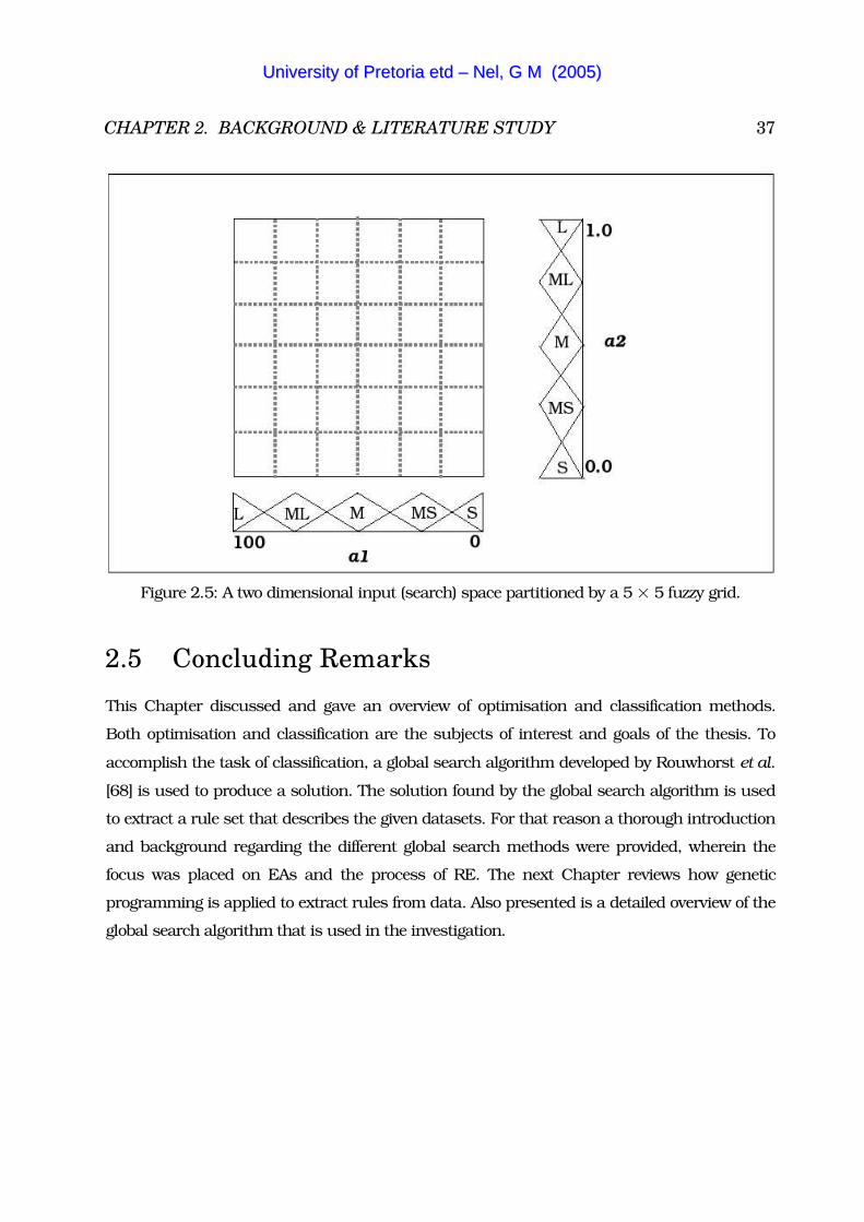
CHAPTER 2. BACKGROUND & LITERATURE STUDY 37
Figure 2.5: A two dimensional input (search) space partitioned by a 5 � 5 fuzzy grid.
2.5 Concluding Remarks
This Chapter discussed and gave an overview of optimisation and classification methods.
Both optimisation and classification are the subjects of interest and goals of the thesis. To
accomplish the task of classification, a global search algorithm developed by Rouwhorst et al.
[68] is used to produce a solution. The solution found by the global search algorithm is used
to extract a rule set that describes the given datasets. For that reason a thorough introduction
and background regarding the different global search methods were provided, wherein the
focus was placed on EAs and the process of RE. The next Chapter reviews how genetic
programming is applied to extract rules from data. Also presented is a detailed overview of the
global search algorithm that is used in the investigation.
UUnniivveerrssiittyy ooff PPrreettoorriiaa eettdd –– NNeell,, GG MM ((22000055))

Chapter 3
Genetic Programming���� �������� �� ����� ������� ������ ����� ���� ���� ����� ���� ��������� ������� � �������
��� ��������������� ������� ����������������������������� �������������������������� ���� �����
����������� ����� !"#������������������������ ����������� ������
3.1 Genetic Programming for RE
Chapter 2 presented the general architecture of an EA, and discussed the evolutionary
operators, strategies and methods used. The evolutionary operators were not specific to any
particular EA paradigm, therefore the evolutionary operators used in GP will be reviewed in
this Chapter. The termination condition, fitness function and general functionality of an EA
have already been reviewed in Chapter 2. The first Section starts by introducing GP. The
Sections that follow describe two representations commonly found in GP. The first
representation to be reviewed describes the process of evolving a program that gives the
correct output for specific inputs. The first representation is also used to discuss the
evolutionary operators used in GP. The second representation is discussed using an example
of a simple classification problem. The problem is then used to discuss the process of rule
extraction.
3.1.1 Introduction
The GP paradigm was derived from GAs by John Koza [46], who wished to create an
algorithm that could evolve a solution program given a set of input values, without explicitly
38
UUnniivveerrssiittyy ooff PPrreettoorriiaa eettdd –– NNeell,, GG MM ((22000055))
CHAPTER 3. GENETIC PROGRAMMING 39
programming the algorithm for a particular solution, i.e. by not telling it how to develop the
program. To represent the set of possible programs, Koza utilised a tree structure
representation, one that provides a convenient way to represent programs, functions rules,
etc., since a tree structure can branch into several hierarchical levels. For example, take a
mathematical function that can be decomposed into hierarchical levels of functions, variables
and constants. The following two Sections discuss how such tree structures are utilised for
two different types of problems.
3.1.2 Evolving a Program and Evolutionary Operators
This Section discusses by means of an example, the representation of an individual for a
mathematical optimisation problem. The representative example involves a given limited
function set, that is used to evolve a function that accurately describes the relationship
between a set of input and target values, i.e. function approximation. The expression tree
individuals produced from the example are used to give an in-depth review regarding the
evolutionary operators mentioned in Chapter 2.
Expression trees representing mathematical expressions can be built using functions that
take either one or two arguments from the function set {�, �, �, �, �} in the internal nodes of
the tree. Examples of such functions that are built while the individual is evolved are given
below. The leaf nodes of the expression trees each contain a value from the terminal set which
consists of variables {a,b,c} and the continuous value z � �. Two nodes in two different
expression trees will have the same arity if the function contained in the node of tree A takes
the same number of arguments as that in the node of tree B. To build an expression tree a
random selection is made for the root node from either the set of functions or the set of
terminals. Note that a root node can be a leaf node for this type of representation, since
simple functions consisting of only a variable exist, for example, ‘a � 1’ represents a straight
line in a two-dimensional Cartesian space, where a is one of the variables.
Assume the addition function operator ‘�’ is chosen as the root node. The addition
function ‘�’ takes two arguments, therefore two choices are made at random from both the
terminal and function sets. Assume that the terminal value, variable ‘a’, is chosen as the first
argument, and multiplication function ‘�’ is chosen as the second argument. The function
‘a � �’ is symbolically expressed in prefix (polish) notation as:
UUnniivveerrssiittyy ooff PPrreettoorriiaa eettdd –– NNeell,, GG MM ((22000055))

CHAPTER 3. GENETIC PROGRAMMING 40
+ a*
The value ‘a’ is a terminal, therefore the node that contains it will be a leaf node. The function
‘�’ is non-terminal, hence another two arguments are randomly chosen from the function and
terminal sets. Figure 3.1 (a) illustrates the expression tree as described above. Assume
terminal ‘c’ and function ‘�’ are chosen as the arguments of ‘�’. The resulting expression tree
is illustrated in Figure 3.1 (b), which is also expressed as:
+ a *c /
Assume that two random selections ‘�’ and ‘�’ are made from the function set, which
represents a split in the branch of the expression tree, since both functions each have two
arguments. The symbolic expression of Figure 3.1 (c) is written as:
+ a *c / *�
Assume that the last multiplication function ‘�’ has two random selections ‘2’ and ‘b’ from the
terminal set as arguments. The square root function ‘�’ can take only one argument, which is
random selection ‘�’. The new symbolic expression is:
+ a *c / *2 b �-
which has the equivalent expression tree in Figure 3.1 (d). The ‘�’ function has two
arguments, which are again chosen at random. Assume that the selections for arguments are
both from the terminal set, being the terminal values ‘c’ and ‘3’ respectively. The resulting
expression tree is given in Figure 3.2, and symbolically expressed in prefix (polish) notation
as:
+ a *c / *2 b � -c 3
UUnniivveerrssiittyy ooff PPrreettoorriiaa eettdd –– NNeell,, GG MM ((22000055))

CHAPTER 3. GENETIC PROGRAMMING 41
The expression tree is complete with all branches terminating in leaf nodes selected from the
terminal set. The function f(a, b, c) represents the expression tree in Figure 3.2:
f a , b ,c �a�c 2 b
� c�3 The expression tree is tested with a dataset of input values for variables {a, b, c} and
corresponding output values which the function is expected to produce. The fitness of the
expression tree (function f(a, b, c)) can be measured relative to all other expression trees
produced by determining the normalised distance of the trees from the target value. This
distance is calculated as the absolute of the difference between the value produced by the
expression tree and the target value.
UUnniivveerrssiittyy ooff PPrreettoorriiaa eettdd –– NNeell,, GG MM ((22000055))
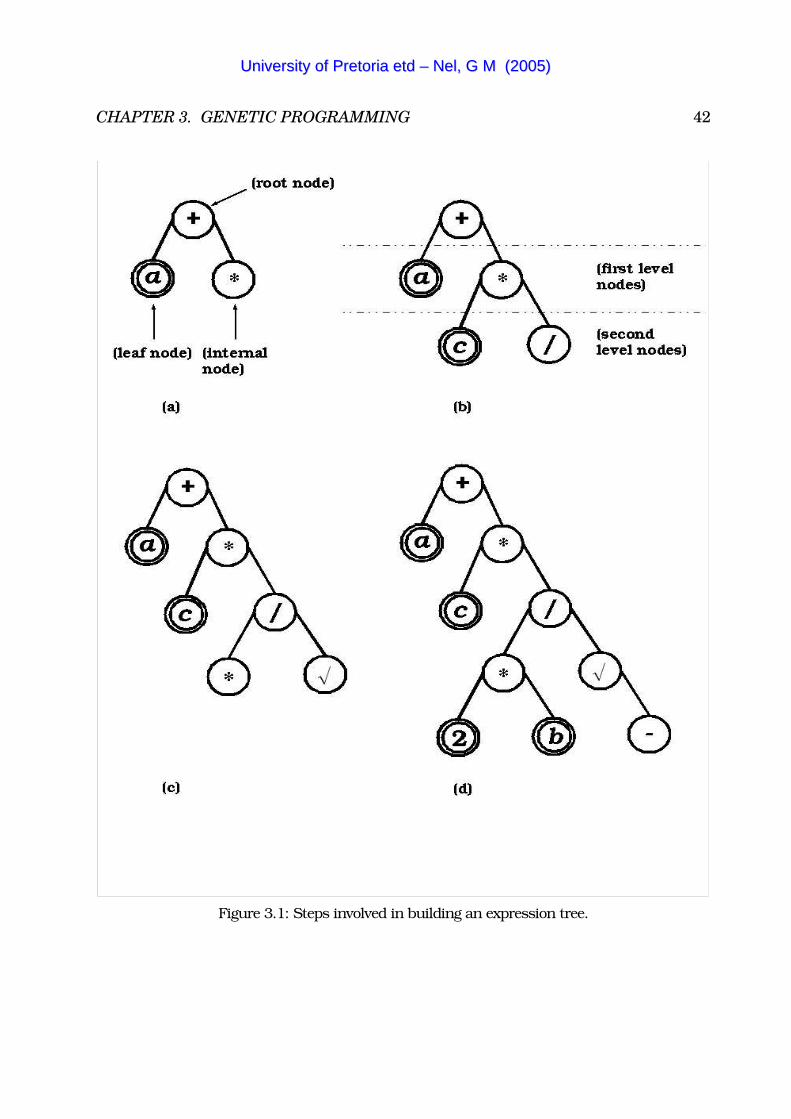
CHAPTER 3. GENETIC PROGRAMMING 42
Figure 3.1: Steps involved in building an expression tree.
UUnniivveerrssiittyy ooff PPrreettoorriiaa eettdd –– NNeell,, GG MM ((22000055))
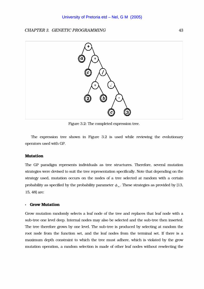
CHAPTER 3. GENETIC PROGRAMMING 43
Figure 3.2: The completed expression tree.
The expression tree shown in Figure 3.2 is used while reviewing the evolutionary
operators used with GP.
Mutation
The GP paradigm represents individuals as tree structures. Therefore, several mutation
strategies were devised to suit the tree representation specifically. Note that depending on the
strategy used, mutation occurs on the nodes of a tree selected at random with a certain
probability as specified by the probability parameter �m . These strategies as provided by [13,
15, 48] are:
� Grow Mutation
Grow mutation randomly selects a leaf node of the tree and replaces that leaf node with a
sub-tree one level deep. Internal nodes may also be selected and the sub-tree then inserted.
The tree therefore grows by one level. The sub-tree is produced by selecting at random the
root node from the function set, and the leaf nodes from the terminal set. If there is a
maximum depth constraint to which the tree must adhere, which is violated by the grow
mutation operation, a random selection is made of other leaf nodes without reselecting the
UUnniivveerrssiittyy ooff PPrreettoorriiaa eettdd –– NNeell,, GG MM ((22000055))
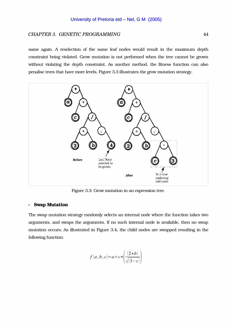
CHAPTER 3. GENETIC PROGRAMMING 44
same again. A reselection of the same leaf nodes would result in the maximum depth
constraint being violated. Grow mutation is not performed when the tree cannot be grown
without violating the depth constraint. As another method, the fitness function can also
penalise trees that have more levels. Figure 3.3 illustrates the grow mutation strategy.
Figure 3.3: Grow mutation in an expression tree.
� Swap Mutation
The swap mutation strategy randomly selects an internal node where the function takes two
arguments, and swaps the arguments. If no such internal node is available, then no swap
mutation occurs. As illustrated in Figure 3.4, the child nodes are swapped resulting in the
following function:
f a , b ,c �a�c 2 b
� 3�c
UUnniivveerrssiittyy ooff PPrreettoorriiaa eettdd –– NNeell,, GG MM ((22000055))
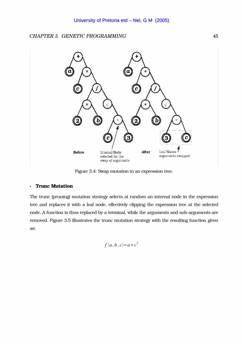
CHAPTER 3. GENETIC PROGRAMMING 45
Figure 3.4: Swap mutation in an expression tree.
� Trunc Mutation
The trunc (pruning) mutation strategy selects at random an internal node in the expression
tree and replaces it with a leaf node, effectively clipping the expression tree at the selected
node. A function is thus replaced by a terminal, while the arguments and sub-arguments are
removed. Figure 3.5 illustrates the trunc mutation strategy with the resulting function given
as:
f a ,b , c �a�c2
UUnniivveerrssiittyy ooff PPrreettoorriiaa eettdd –– NNeell,, GG MM ((22000055))
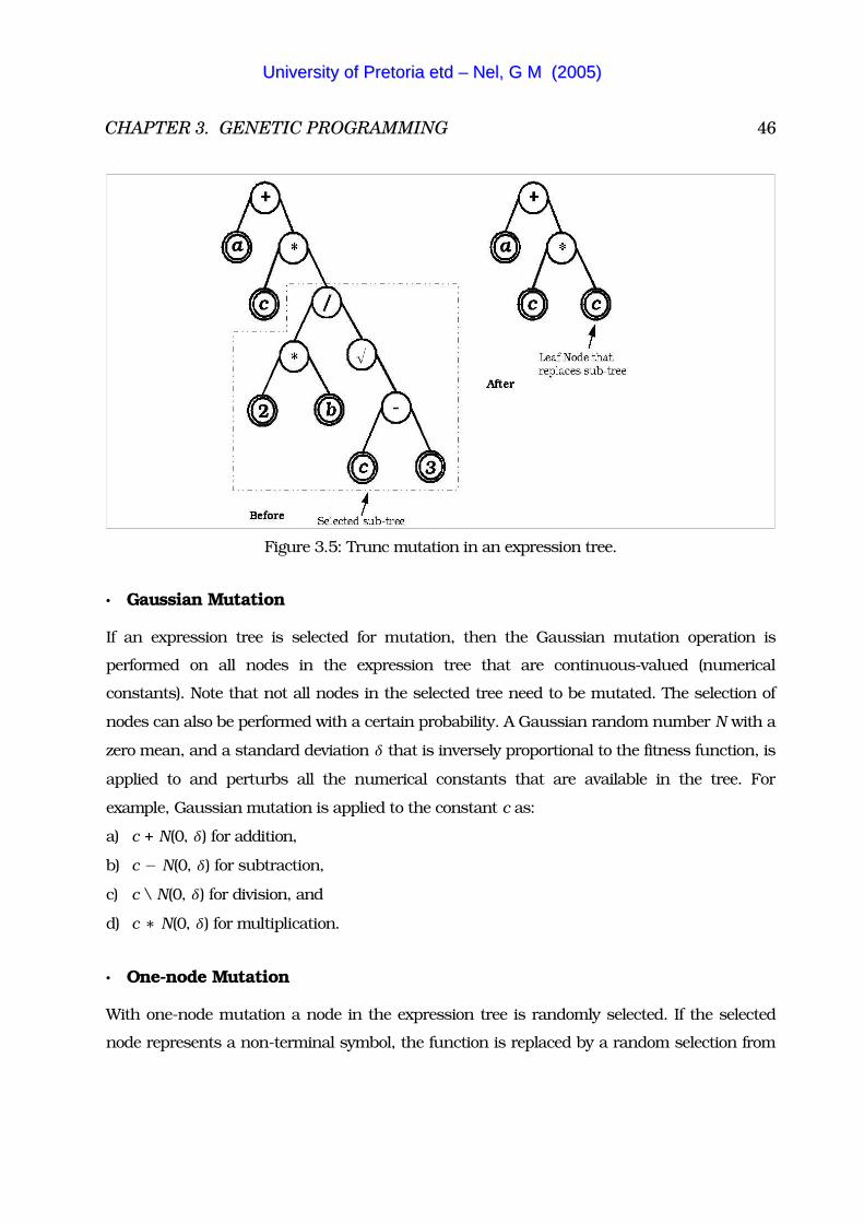
CHAPTER 3. GENETIC PROGRAMMING 46
Figure 3.5: Trunc mutation in an expression tree.
� Gaussian Mutation
If an expression tree is selected for mutation, then the Gaussian mutation operation is
performed on all nodes in the expression tree that are continuous-valued (numerical
constants). Note that not all nodes in the selected tree need to be mutated. The selection of
nodes can also be performed with a certain probability. A Gaussian random number N with a
zero mean, and a standard deviation � that is inversely proportional to the fitness function, is
applied to and perturbs all the numerical constants that are available in the tree. For
example, Gaussian mutation is applied to the constant c as:
a) c � N(0, �) for addition,
b) c � N(0, �) for subtraction,
c) c � N(0, �) for division, and
d) c N(0, �) for multiplication.
� One-node Mutation
With one-node mutation a node in the expression tree is randomly selected. If the selected
node represents a non-terminal symbol, the function is replaced by a random selection from
UUnniivveerrssiittyy ooff PPrreettoorriiaa eettdd –– NNeell,, GG MM ((22000055))
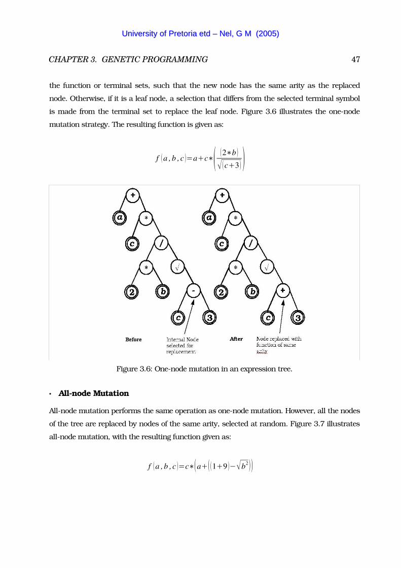
CHAPTER 3. GENETIC PROGRAMMING 47
the function or terminal sets, such that the new node has the same arity as the replaced
node. Otherwise, if it is a leaf node, a selection that differs from the selected terminal symbol
is made from the terminal set to replace the leaf node. Figure 3.6 illustrates the one-node
mutation strategy. The resulting function is given as:
f a , b ,c �a�c 2 b
� c�3
Figure 3.6: One-node mutation in an expression tree.
� All-node Mutation
All-node mutation performs the same operation as one-node mutation. However, all the nodes
of the tree are replaced by nodes of the same arity, selected at random. Figure 3.7 illustrates
all-node mutation, with the resulting function given as:
f a , b , c �c a� 1�9 ��b2
UUnniivveerrssiittyy ooff PPrreettoorriiaa eettdd –– NNeell,, GG MM ((22000055))
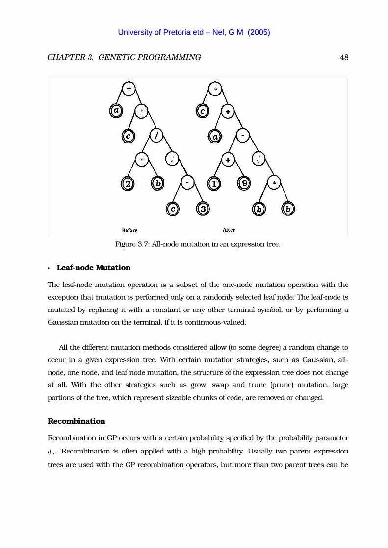
CHAPTER 3. GENETIC PROGRAMMING 48
Figure 3.7: All-node mutation in an expression tree.
� Leaf-node Mutation
The leaf-node mutation operation is a subset of the one-node mutation operation with the
exception that mutation is performed only on a randomly selected leaf node. The leaf-node is
mutated by replacing it with a constant or any other terminal symbol, or by performing a
Gaussian mutation on the terminal, if it is continuous-valued.
All the different mutation methods considered allow (to some degree) a random change to
occur in a given expression tree. With certain mutation strategies, such as Gaussian, all-
node, one-node, and leaf-node mutation, the structure of the expression tree does not change
at all. With the other strategies such as grow, swap and trunc (prune) mutation, large
portions of the tree, which represent sizeable chunks of code, are removed or changed.
Recombination
Recombination in GP occurs with a certain probability specified by the probability parameter
�r . Recombination is often applied with a high probability. Usually two parent expression
trees are used with the GP recombination operators, but more than two parent trees can be
UUnniivveerrssiittyy ooff PPrreettoorriiaa eettdd –– NNeell,, GG MM ((22000055))

CHAPTER 3. GENETIC PROGRAMMING 49
involved in constructing the offspring by selecting portions from the parent trees. Typically,
the parent trees are copied into intermediate individuals, and crossover is performed on the
intermediate individuals so as to produce offspring individuals. Of the crossover methods
mentioned in Chapter 2, the one-point crossover, also known as one-node crossover, is often
applied in GP. One randomly selected node in a parent individual is swapped with the
randomly selected node of another parent individual if the nodes have the same arity. Note
that sub-trees of the nodes are not exchanged. Therefore the tree structures of the parent
individuals and the offspring are equivalent. One-node mutation therefore has the advantage
that the offspring trees need not be pruned if there is a maximum depth constraint in place.
Figure 3.8 illustrates the one-node crossover operation.
The two functions,
f 1 a ,b , c �a�c 2 b
� c�3 and
f 2 a , b , c �2 3
� c�b
produce the offspring functions,
f 1 a , b , c �a�c 2 b � c�3 and
f 2 a ,b ,c � 23 �� c�b
UUnniivveerrssiittyy ooff PPrreettoorriiaa eettdd –– NNeell,, GG MM ((22000055))
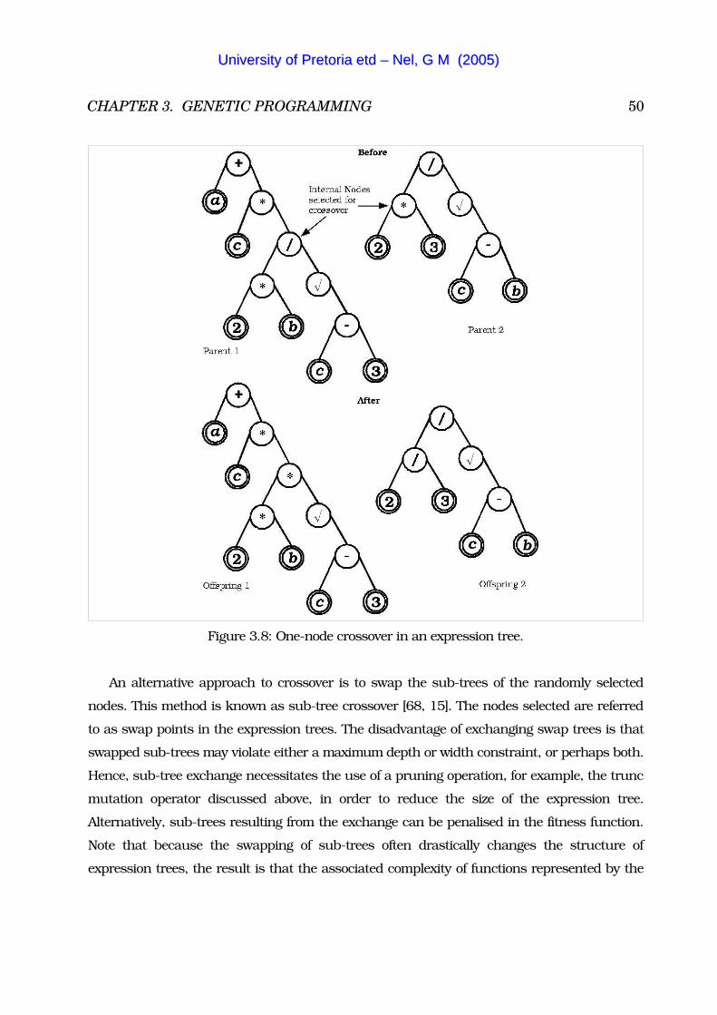
CHAPTER 3. GENETIC PROGRAMMING 50
Figure 3.8: One-node crossover in an expression tree.
An alternative approach to crossover is to swap the sub-trees of the randomly selected
nodes. This method is known as sub-tree crossover [68, 15]. The nodes selected are referred
to as swap points in the expression trees. The disadvantage of exchanging swap trees is that
swapped sub-trees may violate either a maximum depth or width constraint, or perhaps both.
Hence, sub-tree exchange necessitates the use of a pruning operation, for example, the trunc
mutation operator discussed above, in order to reduce the size of the expression tree.
Alternatively, sub-trees resulting from the exchange can be penalised in the fitness function.
Note that because the swapping of sub-trees often drastically changes the structure of
expression trees, the result is that the associated complexity of functions represented by the
UUnniivveerrssiittyy ooff PPrreettoorriiaa eettdd –– NNeell,, GG MM ((22000055))

CHAPTER 3. GENETIC PROGRAMMING 51
trees also alters. Figure 3.9 illustrates the swapping of sub-trees after swap points in the
parent trees were identified. The parent functions,
f 1 a ,b , c �a�c 2 b
� c�3 and
f 2 a , b , c �2 3
� c�b
produce the offspring functions,
f 1 a , b , c �a�c 2 3 and
f 2 a , b , c � 2 b
� c�3 �� c�b
UUnniivveerrssiittyy ooff PPrreettoorriiaa eettdd –– NNeell,, GG MM ((22000055))
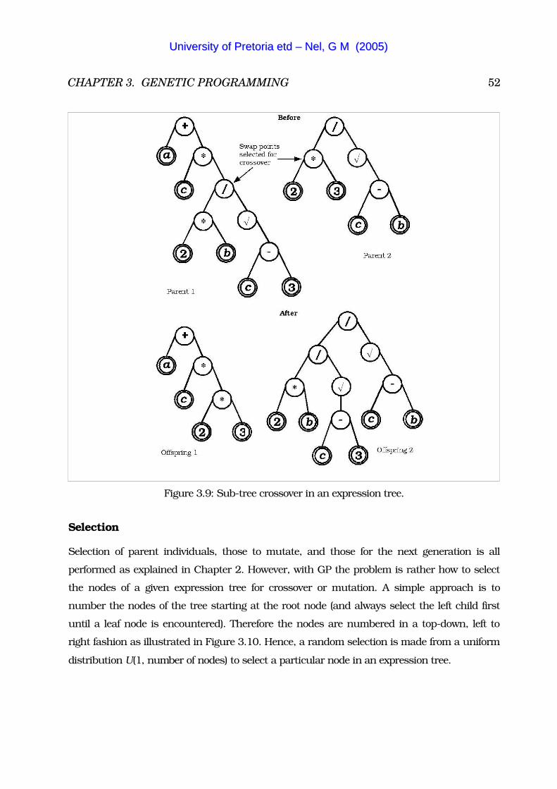
CHAPTER 3. GENETIC PROGRAMMING 52
Figure 3.9: Sub-tree crossover in an expression tree.
Selection
Selection of parent individuals, those to mutate, and those for the next generation is all
performed as explained in Chapter 2. However, with GP the problem is rather how to select
the nodes of a given expression tree for crossover or mutation. A simple approach is to
number the nodes of the tree starting at the root node (and always select the left child first
until a leaf node is encountered). Therefore the nodes are numbered in a top-down, left to
right fashion as illustrated in Figure 3.10. Hence, a random selection is made from a uniform
distribution U(1, number of nodes) to select a particular node in an expression tree.
UUnniivveerrssiittyy ooff PPrreettoorriiaa eettdd –– NNeell,, GG MM ((22000055))
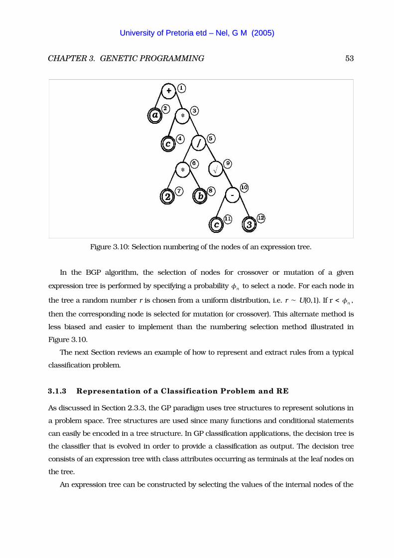
CHAPTER 3. GENETIC PROGRAMMING 53
Figure 3.10: Selection numbering of the nodes of an expression tree.
In the BGP algorithm, the selection of nodes for crossover or mutation of a given
expression tree is performed by specifying a probability �n to select a node. For each node in
the tree a random number r is chosen from a uniform distribution, i.e. r � U(0,1). If r � �n ,
then the corresponding node is selected for mutation (or crossover). This alternate method is
less biased and easier to implement than the numbering selection method illustrated in
Figure 3.10.
The next Section reviews an example of how to represent and extract rules from a typical
classification problem.
3.1.3 Representation of a Classification Problem and RE
As discussed in Section 2.3.3, the GP paradigm uses tree structures to represent solutions in
a problem space. Tree structures are used since many functions and conditional statements
can easily be encoded in a tree structure. In GP classification applications, the decision tree is
the classifier that is evolved in order to provide a classification as output. The decision tree
consists of an expression tree with class attributes occurring as terminals at the leaf nodes on
the tree.
An expression tree can be constructed by selecting the values of the internal nodes of the
UUnniivveerrssiittyy ooff PPrreettoorriiaa eettdd –– NNeell,, GG MM ((22000055))
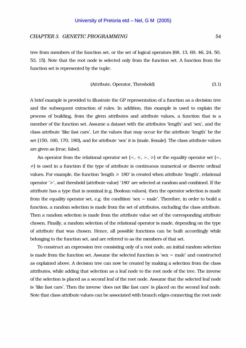
CHAPTER 3. GENETIC PROGRAMMING 54
tree from members of the function set, or the set of logical operators [68, 13, 69, 46, 24, 50,
53, 15]. Note that the root node is selected only from the function set. A function from the
function set is represented by the tuple:
(Attribute, Operator, Threshold) (3.1)
A brief example is provided to illustrate the GP representation of a function as a decision tree
and the subsequent extraction of rules. In addition, this example is used to explain the
process of building, from the given attributes and attribute values, a function that is a
member of the function set. Assume a dataset with the attributes ‘length’ and ‘sex’, and the
class attribute ‘like fast cars’. Let the values that may occur for the attribute ‘length’ be the
set {150, 160, 170, 180}, and for attribute ‘sex’ it is {male, female}. The class attribute values
are given as {true, false}.
An operator from the relational operator set {�, �, �, �} or the equality operator set {�,
�} is used in a function if the type of attribute is continuous numerical or discrete ordinal
values. For example, the function ‘length � 180’ is created when attribute ‘length’, relational
operator ‘�’, and threshold (attribute value) ‘180’ are selected at random and combined. If the
attribute has a type that is nominal (e.g. Boolean values), then the operator selection is made
from the equality operator set, e.g. the condition ‘sex � male’. Therefore, in order to build a
function, a random selection is made from the set of attributes, excluding the class attribute.
Then a random selection is made from the attribute value set of the corresponding attribute
chosen. Finally, a random selection of the relational operator is made, depending on the type
of attribute that was chosen. Hence, all possible functions can be built accordingly while
belonging to the function set, and are referred to as the members of that set.
To construct an expression tree consisting only of a root node, an initial random selection
is made from the function set. Assume the selected function is ‘sex � male’ and constructed
as explained above. A decision tree can now be created by making a selection from the class
attributes, while adding that selection as a leaf node to the root node of the tree. The inverse
of the selection is placed as a second leaf of the root node. Assume that the selected leaf node
is ‘like fast cars’. Then the inverse ‘does not like fast cars’ is placed on the second leaf node.
Note that class attribute values can be associated with branch edges connecting the root node
UUnniivveerrssiittyy ooff PPrreettoorriiaa eettdd –– NNeell,, GG MM ((22000055))

CHAPTER 3. GENETIC PROGRAMMING 55
with leaf nodes. Figure 3.11 (a) illustrates the expression and resulting decision tree according
to the example. Using the format of the rule provided in equation (2.1) of Section 2.4.2, two
rules can be extracted from the decision tree. A rule is constructed by replacing the
antecedent of the rule with the function in the root node, along with the class attribute value
on the associated branch edge. The consequence is replaced by the leaf node, which is the
associated class attribute. Therefore, the rule ‘IF sex � male THEN like fast cars’ can be
extracted. The rule that can be extracted from the second leaf node is ‘IF sex � male THEN
does not like fast cars’. The rules describe the relationship between the ‘sex’ attribute and the
class attribute ‘like fast cars’. Therefore, the path from the root node to one of the leaf nodes
of a decision tree represents a rule that can be extracted from the decision tree.
A decision tree with higher complexity can be created by combining more of the existing
functions with the decision tree described above. Note that the discrete operator ‘AND’ is
implicit between the nodes of the expression tree within each branch. The discrete operator
‘OR’ is implicit between the branches of the expression tree. Therefore, an expression tree can
be grown by replacing the leaf nodes with more functions (as internal nodes to the tree). In
order to grow the example expression tree, two internal nodes are added one level below the
root node, i.e. the second level. Thus, the leaf nodes of the decision tree are replaced with new
internal nodes. Hence, random functions in the new nodes on the second level are joined to
the existing function in the root node. Assume that the new functions that randomly replace
the two leaf nodes as two new internal nodes in the second level are ‘length � 180’ and
‘length � 170’. Finally, two leaf nodes are added to each internal node of the expression tree
in similar way as explained above in order to create a new decision tree. Now four new rules
can be extracted from the newly grown decision tree. By following the path from root node to
leaf node of the tree indicated by (i) in Figure 3.11 (b), the rule ‘IF sex � male AND length �
180 THEN does not like fast cars’ can be extracted. Figure 3.11 (b) illustrates the resulting
decision tree that was grown in the given example, as well as the four rules that can be
extracted as has been explained.
UUnniivveerrssiittyy ooff PPrreettoorriiaa eettdd –– NNeell,, GG MM ((22000055))
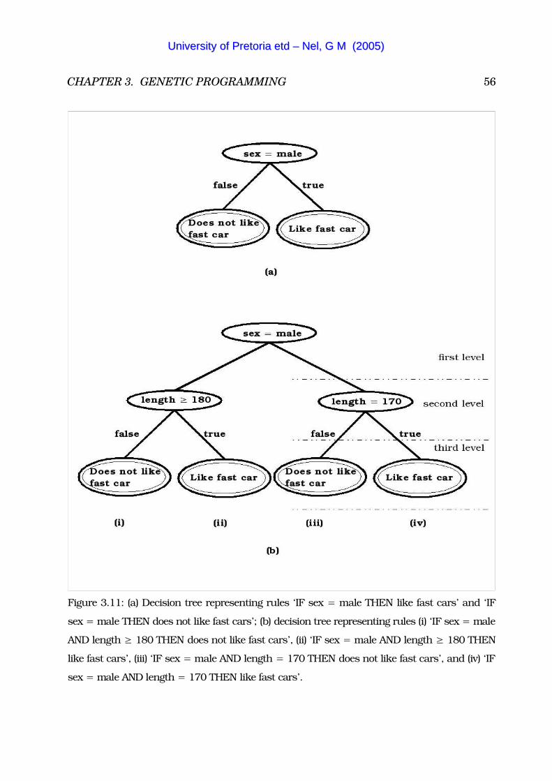
CHAPTER 3. GENETIC PROGRAMMING 56
Figure 3.11: (a) Decision tree representing rules ‘IF sex � male THEN like fast cars’ and ‘IF
sex � male THEN does not like fast cars’; (b) decision tree representing rules (i) ‘IF sex � male
AND length � 180 THEN does not like fast cars’, (ii) ‘IF sex � male AND length � 180 THEN
like fast cars’, (iii) ‘IF sex � male AND length � 170 THEN does not like fast cars’, and (iv) ‘IF
sex � male AND length � 170 THEN like fast cars’.
UUnniivveerrssiittyy ooff PPrreettoorriiaa eettdd –– NNeell,, GG MM ((22000055))
CHAPTER 3. GENETIC PROGRAMMING 57
Functions from the function set, with values from the class attribute set, are used to build
expression trees. The GP algorithm itself evolves, evaluates and selects by means of
evolutionary operators the different solutions in the search space of classifiers to the specific
problem.
Section 3.2 discusses the particular GP implementation that makes use of the building
block hypothesis [68, 69]. Most of the concepts reviewed in Section 3.1 are not considered in
Section 3.2 due to these concepts’ similarity. The unique differences between the building
block approach to GP for decision tree construction and standard GP are also discussed.
3.2 Building Block Approach to GP
The building block approach to genetic programming (BGP) has been developed specifically to
evolve decision trees for extracting rules from data [68, 69]. The main objective of the building
block approach is to construct solutions incrementally, starting from simple solutions,
increasing the complexity of individuals where needed. The building block approach is trying
mainly to achieve one of the objectives of RE, namely to produce simple rules. This Section
gives an overview of BGP as follows: Section 3.2.1 provides a philosophical discussion of the
building block approach. A summary of critique against BGP is presented in Section 3.2.2.
Sections 3.2.3 to 3.2.12 review the general architecture, fitness function, operators,
termination criteria, and strategies used with BGP.
3.2.1 Philosophical Motivation for the Building Block Hypothesis
Humans have, over time, evolved several approaches to solving complex problems. One
technique is to reduce such problems to simpler, more manageable ones that can then be
solved more easily, or for which the solution is already known. In order to survive and
prosper, humans have also developed skills to identify and recall problems and their solutions
(concepts). The process of identifying and recalling problems and their solutions is generally
known as gaining experience (learning).
The learning process occurs mainly in three ways, namely learning of concepts through
one’s own experience, learning of concepts by example, or through being taught such
concepts. In order to illustrate the learning processes, consider the example of one’s hand
being burnt by fire. Own experience is gained by burning one’s hand with fire. Seeing how
UUnniivveerrssiittyy ooff PPrreettoorriiaa eettdd –– NNeell,, GG MM ((22000055))

CHAPTER 3. GENETIC PROGRAMMING 58
someone gets his/her hand burned by fire illustrates gaining experience by example. By being
told that fire will burn one’s hand illustrates the gain of experience by being taught, without
ever having to experience personally the pain of being burnt by fire. Whichever way the
experience may be gained, the concept that fire will burn one’s hand is a necessary
experience (building block) that ultimately can influence the success and prosperity of any
human.
As an example of how building blocks can help a human to overcome a complex situation,
consider the problem of finding one’s way along the streets of an unfamiliar city. There is
most probably no pre-written rule set for the person who needs to travel from point A to point
B. However, by reducing the problem, and by recalling all previous experience concerning
cities, streets and directions, a person can quickly devise a set of plausible actions to take.
The reduced pieces (previous experiences or solutions to problems) are the building blocks
that a person uses to solve the problem at hand. The order in which a person uses the
building blocks to solve the problem is arbitrary. Therefore, building blocks can appear in any
combination. They can also be re-used in a variety of problems and situations.
Since the combination of building blocks is arbitrary, a variety of solutions arise by
combining building blocks. Certain combinations, rather than others, may produce less
successful solutions. A combination of building blocks may, in fact, also produce a new
building block at a higher level, which itself may be used in combination with other building
blocks in order to solve a problem. Elementary building blocks that can not be further
reduced into lower-level building blocks must be highly precise blocks, i.e. the elementary
blocks should be quite accurate and thereby useful [62, 75].
In order to find the best combination of building blocks, the widely accepted principle of
parsimony, i.e. Ockham’s razor [80], is the general accepted rule of thumb. Ockham’s razor
states that simpler explanations are preferable to more complex explanations of the same
phenomena. Generally it is easier for people to understand simpler explanations than those
that are more complex. Therefore, simplicity itself is more desirable for reasons of
comprehension. However, simplicity need not always coincide with generalisation [13]. For
example, a single simplistic building block in the BGP algorithm is not necessarily an
accurate solution, as the simplified decision tree it represents may not correctly classify all the
data instances. In other words, the single simplistic building block may be less capable of
generalising the data. Note that it is the ultimate goal of BGP to evolve the simplest and
UUnniivveerrssiittyy ooff PPrreettoorriiaa eettdd –– NNeell,, GG MM ((22000055))
CHAPTER 3. GENETIC PROGRAMMING 59
optimal combination of building blocks that generalise complex problems well.
The advantages of BGP include the following:
� RE from BGP is simple since BGP is a specific implementation of GP where rules are easily
extracted from the representation of individuals in the population, as seen in Section 3.1.3
above.
� BGP produces the simplest and shortest possible decision trees, and therefore rules
extracted are also simple and short.
� Convergence in BGP occurs quickly because one starts with less degree of freedom. The
expression trees are ‘grown’ from the building blocks that ‘survive’ each generation, hence
they are the fittest in each generation.
3.2.2 Building Block Hypothesis Critique
The building block hypothesis is not without criticism. Researchers such as O’Reilly et al.
[62], Thornton [75] and Forrest et al. [28] question the usefulness and credibility of the
building block hypothesis. Using their interpretations of the GP schema theorem, O’Reilly et
al. defined the building block hypothesis (BBH) as a hierarchical search by GP through the
combination of building blocks. O’Reilly et al. then reported that they found that the BBH
was not convincing for several reasons, namely [62]
� that it is difficult to find support for the promotion and combination of building blocks
solely by rigorous interpretation of a GP schema theorem;
� even if there were support for a BBH, it is empirically questionable whether building blocks
always exist because partial solutions of consistently above average fitness and resilience
to disruption in the individuals are not assured; and
� the BBH constitutes a narrow and imprecise account of GP search behaviour.
O’Reilly et al. reported that the most serious issue concerns the time-dependent
behaviour of schema disruption of individuals in the population. In other words, the internal
structure (schema) of individuals (the decision trees) constantly changes due to evolutionary
processes. Hence, the question to be asked is whether building blocks for the expression and
the resulting decision trees had ever really been found. The observed discrepancy between the
average fitness of individuals relative to the population fitness supports the time-dependent
behaviour of schema disruption. The caution clearly stated by O’Reilly et al. is that there are
UUnniivveerrssiittyy ooff PPrreettoorriiaa eettdd –– NNeell,, GG MM ((22000055))
CHAPTER 3. GENETIC PROGRAMMING 60
times that the BBH will not be applicable, because the BBH presupposes the existence of
building blocks in the underlying data, despite the fact that compactness and consistent
fitness are not guaranteed in the individuals.
O’Reilly et al. conclude that a major problem of BBH algorithms and GP in general, is that
BBH algorithms exert no control over the building blocks in individuals that are modified by
the evolutionary operators. The selection of the building blocks that is modified is a stochastic
selection process, meaning that the fitter building blocks in an individual also have a chance
to be altered, rather than selecting exclusively only the less fit blocks. O’Reilly et al.
introduced the term disruption probability to describe the uncertainty of selecting fit building
blocks over those that are less fit. Another critique is that the probability of disruption of a
schema (the structure of an individual) changes over time and is unpredictable, even from
one generation to the next. O’Reilly et al. suggest that a more useful and precise building
block definition must also state something about the time-dependent behaviour of the
probability of disruption as discussed. In other words, a guarantee must be provided
regarding the fitness of building blocks. The building blocks that are fit either must not
change, or, if they are changed, the fitness of the modified or new building blocks must be
optimal. This thesis intends to provide a method that guarantees the optimality of building
blocks used by the building block hypothesis.
3.2.3 General Architecture and Representation
The BGP algorithm as presented by [68] is shown in Figure 3.12.
Recall from Section 3.1 that GP uses hierarchical computer programs that are represented as
tree structures. BGP is a special implementation of GP, hence BGP also uses tree structures
as the individuals of a population. A tree structure in GP is feasible when the solution
represented by the tree structure adheres to the constraints of its representation. So does the
example tree given in Section 3.1.1 adhere to mathematical constraints, while that given in
Section 3.1.2 adheres to discrete and relational constraints in order to be valid
representations. Because the goal of BGP is to find the simplest optimal combination of
building blocks, BGP builds tree structures starting from the simplest feasible trees that can
be constructed in terms of hierarchical tree levels and complexity.
UUnniivveerrssiittyy ooff PPrreettoorriiaa eettdd –– NNeell,, GG MM ((22000055))
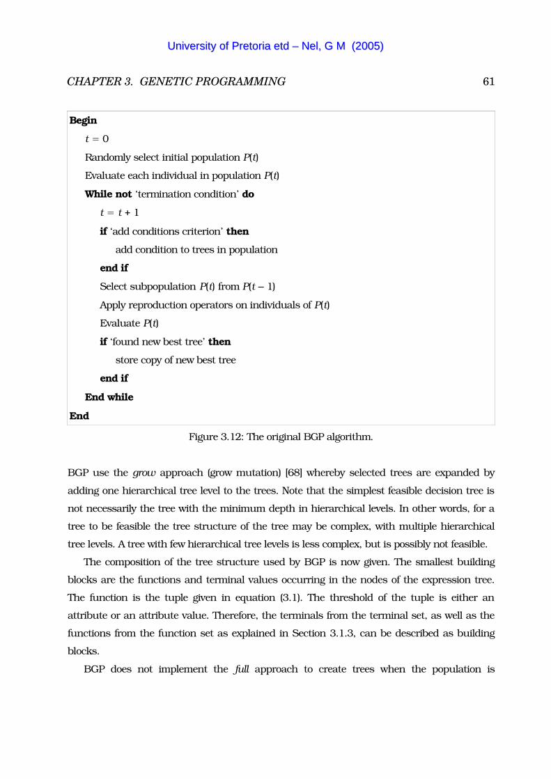
CHAPTER 3. GENETIC PROGRAMMING 61
Begin
t � 0
Randomly select initial population P(t)
Evaluate each individual in population P(t)
While not ‘termination condition’ do
t � t � 1
if ‘add conditions criterion’ then
add condition to trees in population
end if
Select subpopulation P(t) from P(t � 1)
Apply reproduction operators on individuals of P(t)
Evaluate P(t)
if ‘found new best tree’ then
store copy of new best tree
end if
End while
End
Figure 3.12: The original BGP algorithm.
BGP use the grow approach (grow mutation) [68] whereby selected trees are expanded by
adding one hierarchical tree level to the trees. Note that the simplest feasible decision tree is
not necessarily the tree with the minimum depth in hierarchical levels. In other words, for a
tree to be feasible the tree structure of the tree may be complex, with multiple hierarchical
tree levels. A tree with few hierarchical tree levels is less complex, but is possibly not feasible.
The composition of the tree structure used by BGP is now given. The smallest building
blocks are the functions and terminal values occurring in the nodes of the expression tree.
The function is the tuple given in equation (3.1). The threshold of the tuple is either an
attribute or an attribute value. Therefore, the terminals from the terminal set, as well as the
functions from the function set as explained in Section 3.1.3, can be described as building
blocks.
BGP does not implement the full approach to create trees when the population is
UUnniivveerrssiittyy ooff PPrreettoorriiaa eettdd –– NNeell,, GG MM ((22000055))
CHAPTER 3. GENETIC PROGRAMMING 62
initialised. With the full approach the trees in the initial population are initialised to a
predetermined maximum depth in hierarchical levels and a maximum width in terms of tree
branches that may be present. Note that the full approach method defies one of the goals of
BGP by producing complex tree structures in the initial population. The only exception where
the full approach method does not defy BGP is in the case where maximum depth in
hierarchical levels is set to be one level deep. The tree structures are all complex because they
are similar in structure and build to the maximum permissible depth and width levels that
are provided as input parameters. Therefore, the full approach does not per definition use
‘building blocks’ in the individuals of the initial population, or any subsequent generations as
does BGP. The latter depend rather on the grow approach, where the initial population of
trees is selected with a minimum tree depth.
Another approach to initialise the first population in GP is the half-and-half method. With
this method half of the population is initialised using the full approach, while the remaining
half is initialised using the grow approach. BGP avoids the half-and-half method, since half
the population would be initialised to the predetermined maximum depth in hierarchical
levels. The BGP algorithm using the half-and-half or full method has less chance to produce
the simplest possible solutions to the problem than the BGP algorithm that employs the grow
approach. The initialisation of the first generation is hereafter explained using the grow
approach.
3.2.4 Initialisation of Population
For the initial population BGP creates expression trees that consist, if possible, of only a root
node (a function from the function set). The leaves of the trees are then randomly selected
from the class attribute set, which is also known as the terminal set. Note that random
selections from the terminal set are for each respective tree during the initialisation process.
The selection for a tree from the terminal set is added as one terminal leaf node to the tree.
The inverse for the selected terminal value is added to the same tree as the second terminal
leaf node to create a decision tree. If the solution represented by the tree is feasible, then the
decision tree created is added as an individual to the initial population. If an infeasible
decision tree is produced, then a different random selection is made from the terminal set.
Both the new terminal value and its inverse replace the previous leaf node values on the tree.
UUnniivveerrssiittyy ooff PPrreettoorriiaa eettdd –– NNeell,, GG MM ((22000055))
CHAPTER 3. GENETIC PROGRAMMING 63
The described process repeats itself until an initial population of feasible individuals is
selected. It is the aim of the initialisation operation in BGP to produce feasible decision trees
in the initial population that contain only one root node, along with two leaf nodes.
3.2.5 Fitness Evaluation
The next step of the algorithm in Figure 3.12 is the evaluation of fitness of the individuals.
The goal of the fitness function is to determine the accuracy of the decision trees. Hence, the
fitness function is a measure that quantifies how well the individuals fit the data in the
current generation. The fitness function measures the fitness of each individual as the
accuracy of the extracted rule set S on the data from the corresponding decision tree. S
consist of all the extracted rules that can be found in a decision tree by following all routes
from the root node to each leaf node. Rouwhorst et al. [68] define the fitness function F(S)
over a rule set, S, as:
F S � MIN� r�S
Accuracy r (3.2)
where Accuracy(r) is the accuracy of a single rule, r. Rule accuracy is expressed as the
average number of instances correctly covered by rule r, i.e.
Accuracy r ��i�1
P
ci �P (3.3)
where ci is 1, if instance i is correctly classified by rule r, and 0 if not. As can be seen from
equation (3.2), the accuracy of the whole rule set is quantified as the accuracy of the worst
rule. The advantage of determining fitness, as indicated by equation (3.2), is that an individual
is penalised if found to contain a rule with low accuracy relative to rules contained in other
individuals. An individual with a useless rule has a higher probability of not surviving to the
next generation, even though the average fitness over all the rules in the rule set is better than
that of other individuals. The disadvantage is that the same individual that is discarded may
also contain a rule which is highly accurate. Another disadvantage of equation (3.2) is that the
UUnniivveerrssiittyy ooff PPrreettoorriiaa eettdd –– NNeell,, GG MM ((22000055))
CHAPTER 3. GENETIC PROGRAMMING 64
algorithm may take longer than necessary to converge, because accurate rules may be lost as
described above.
Alternately, the fitness value of an individual can be calculated as:
F S � MAX� r�S
Accuracy r (3.4)
As can be seen from equation (3.4), the accuracy of the whole rule set is determined by the
rule that has the highest accuracy on the data instances in the training set. An advantage of
equation (3.4) is that an individual that contains a rule with high accuracy stands a better
chance of being selected for the next generation, and, therefore, the rule is not lost. One
disadvantage of equation (3.4) is that there may be a rule in the set of rules of an individual
that is completely inaccurate. Another problem of equation (3.4) is that the average rule
accuracy can be low, but the individual would still be selected for the next generation if that
individual has one very accurate rule. An additional problem that equation (3.4) has is that
the fitness function will cause the algorithm to converge quickly and prematurely to a
solution, because the measurement of fitness is performed on only one rule in the rule set.
A skewness is inherent in both equations (3.2) and (3.4) because preference is given to one
rule in each individual of a population. In other words, the resulting skewness in fitness value
calculation can cause fit decision trees to be discarded unnecessarily or changed, or it can
prevent the algorithm from a timely termination. A method by which to counter the effects of
the skewness problem is to calculate an individual’s average rule accuracy and give that as its
fitness value. Hence, a less accurate rule can be balanced against a more accurate rule. An
individual is measured, therefore, on the accuracy of all the rules it possesses. Thus, an
alternative approach to calculating the fitness of an individual is to calculate the average
fitness of the rules in the rule set, i.e.
F S ��� r�S
Accuracy r
�S�(3.5)
The BGP algorithm provided by Rouwhorst et al. [68] use equation (3.5) to calculate the
fitness of each individual. The fitness of the population is therefore the mean fitness of all its
UUnniivveerrssiittyy ooff PPrreettoorriiaa eettdd –– NNeell,, GG MM ((22000055))
CHAPTER 3. GENETIC PROGRAMMING 65
members. Note that the fitness calculation has no measure by which to evaluate the
complexity of the rule set. This complexity is indicated by the number of conjunctions in the
rule antecedent of each rule in the set. Rule set complexity is therefore a function of the
number of levels in a tree. A rule in the rule set may consist of several conjunctions of
conditions (‘selectors’), but some of those in a rule may be obsolete. If a rule has more
selectors, then it will be more specific, which may lead to a rule that over-fits the data.
Remember that one of the goals of BGP is to extract rules which are the simplest possible.
The BGP algorithm uses the grow approach as explained in Section 3.2.3, whereby the
simplest possible initial solutions (individuals) are chosen, which become incrementally more
complex only if no feasible solution is found. Therefore, no measure of complexity is required
because the individuals are as simple as possible. Crossover may cause the complexity of the
individuals to increase, but BGP subsequently uses, if necessary, a pruning operation on the
offspring individuals to reduce the complexity.
3.2.6 Termination Condition
The evolutionary process continues until either a stopping or converging criterion has been
satisfied. As stopping criterion the algorithm is allowed to run for a maximum number of
generations. When that has been exceeded, the best individual is selected as the solution. It
must be kept in mind that the selected solution may be inaccurate, because the maximum
number of generations may have been reached before convergence actually occurred. In
addition to the stopping criterion, the algorithm stops when the fitness of the best individual
is acceptable, i.e. exceeds a user-specified accuracy threshold.
The termination criterion used by BGP is based on the temperature function used in
simulated annealing [1, 29] wherein an object has a high temperature at time 0, which
decreases with time as an exponential function. Analogue to simulated annealing, BGP starts
with a high fitness goal, which is to obtain an individual with maximum average accuracy in
its rule set. The fitness goal then decreases over time exponentially. BGP, however, is
generation-dependent, which is time-dependent to some extent. In other words, as the
number of generations in BGP increases, so the fitness goal for BGP decreases. The amount
with which the fitness goal is reduced initially decreases slowly. Only when the algorithm has
reached almost the maximum allowable generations is there a drastic reduction in the fitness
UUnniivveerrssiittyy ooff PPrreettoorriiaa eettdd –– NNeell,, GG MM ((22000055))
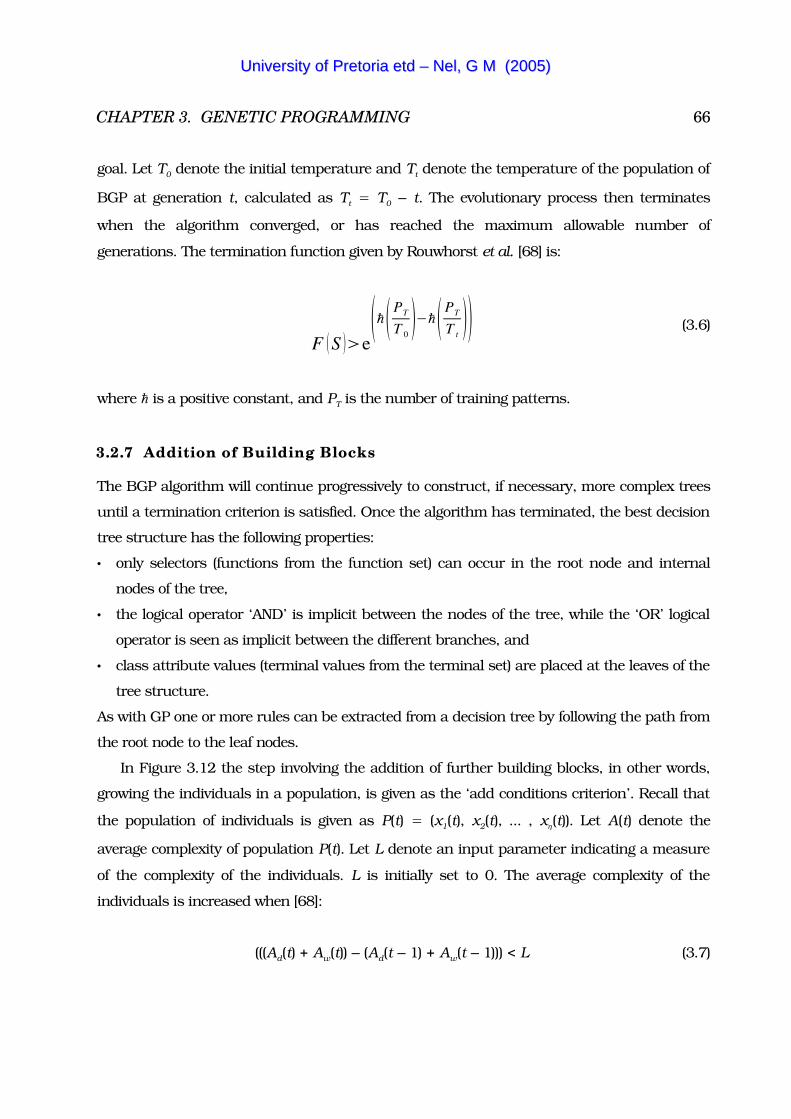
CHAPTER 3. GENETIC PROGRAMMING 66
goal. Let T0 denote the initial temperature and Tt denote the temperature of the population of
BGP at generation t, calculated as Tt � T0 � t. The evolutionary process then terminates
when the algorithm converged, or has reached the maximum allowable number of
generations. The termination function given by Rouwhorst et al. [68] is:
F S �e� PT
T 0�� PT
T t (3.6)
where � is a positive constant, and PT is the number of training patterns.
3.2.7 Addition of Building Blocks
The BGP algorithm will continue progressively to construct, if necessary, more complex trees
until a termination criterion is satisfied. Once the algorithm has terminated, the best decision
tree structure has the following properties:
� only selectors (functions from the function set) can occur in the root node and internal
nodes of the tree,
� the logical operator ‘AND’ is implicit between the nodes of the tree, while the ‘OR’ logical
operator is seen as implicit between the different branches, and
� class attribute values (terminal values from the terminal set) are placed at the leaves of the
tree structure.
As with GP one or more rules can be extracted from a decision tree by following the path from
the root node to the leaf nodes.
In Figure 3.12 the step involving the addition of further building blocks, in other words,
growing the individuals in a population, is given as the ‘add conditions criterion’. Recall that
the population of individuals is given as P(t) � (x1(t), x2(t), ... , x (t)). Let A(t) denote the
average complexity of population P(t). Let L denote an input parameter indicating a measure
of the complexity of the individuals. L is initially set to 0. The average complexity of the
individuals is increased when [68]:
(((Ad(t) � Aw(t)) � (Ad(t � 1) � Aw(t � 1))) � L (3.7)
UUnniivveerrssiittyy ooff PPrreettoorriiaa eettdd –– NNeell,, GG MM ((22000055))
CHAPTER 3. GENETIC PROGRAMMING 67
where Ad(t) is the average depth of the trees in the current generation at time t, and Aw(t) is
the average width. By manipulating the value of parameter L, a variation in the average
complexity, as well as a variation in the average fitness of the population is achieved. For
example, if the average fitness of the population does not improve, L is increased and that in
turn will allow the complexity of the decision trees to be increased by adding more selectors as
internal nodes. The rule in equation (3.7) determines the difference between the current
generation’s average tree width and depth and the previous generation’s average tree width
and depth. If the difference is less than L, then a randomly constructed condition is added to
every stochastically chosen individual in the population. Note that the chosen individuals
must still be feasible, as explained in Section 3.2.3, after the addition of the random
condition. The parameter L is set as a function of the rate of change in average fitness values
of the current and previous generations. In other words, if the rate of change of the average
fitness of the population is large, then the value of L is reduced. For example, assume that the
average fitness value of the current population has improved from the previous generation.
Then very little change in the complexity of the decision tree structure of the population is
required because the population’s average fitness has improved. However, if the current
generation does not improve the average fitness of the population, but decreases or stays
unchanged, then parameter L can be increased to facilitate a change in the complexity of
decision trees in the population. The increase of the complexity of individuals implies that
more building blocks are allowed to be added to the individuals, which may improve the
classification ability of the individuals. If more branches are added to an individual, then more
rules can be extracted while the associated tree width complexity is increased.
3.2.8 Selection
BGP uses the second variation of the tournament selection operation as described in Section
2.3.7. A sample of n individuals is selected at random, and the individual with the best fitness
declared the winner of the tournament. A small value of n causes more random selection to
occur, while a large value of n leads to increased selection pressure. In terms of the latter it is
meant that the better individuals in terms of fitness value will have a better chance of being
selected. The selection operator is used in order to:
� select parents for recombination to produce offspring;
UUnniivveerrssiittyy ooff PPrreettoorriiaa eettdd –– NNeell,, GG MM ((22000055))
CHAPTER 3. GENETIC PROGRAMMING 68
� select individual decision trees for the mutation operation;
� select individual decision trees for the pruning operation; and
� select the individuals to survive to the next generation.
Note that tournament selection reduces the chance of selecting individuals that have bad
fitness values, while improving the chances of selecting individuals with better fitness values
depending on the value of n. Although tournament selection is used as the selection operator
by BGP, any other selection strategy could have been applied.
3.2.9 Mutation
Three mutation operator schemes are defined and used to alter the selected decision trees
[68].
The different mutation operators that are implemented in BGP are as follows.
� Attribute mutation: the attribute of a tuple is mutated by selecting a new attribute from the
set of available attributes. Attribute mutation occurs at probability �attr ;
� Relational operator mutation: the relational operator of a tuple is mutated by selecting a
new operator from the set of available relational operators. Relational operator mutation
occurs at probability �rel ;
� Threshold mutation: the threshold of a tuple is mutated by selecting a new threshold
either from the attribute or a value from the attribute’s domain. Threshold mutation
occurs at probability �thres .
The objective of the mutation schemes is to encourage diversity in the population by
introducing new genetic building blocks, thereby increasing the effectiveness of the search.
The mutation operator schemes are applied probabilistically and are controlled by means of
user-provided probability parameters. In other words, for the mutation operators each node
in the decision tree has a probability to be mutated for each of the mutation schemes. To aid
in the decision as to whether a particular node is to be mutated using a specific mutation
scheme, a random number, !, is sampled from a uniform distribution, U(0, 1). If ! is less
than the corresponding mutation probability, then the corresponding mutation is performed.
Let �rel be the probability parameter that controls the probability to mutate the relational
operator of the tuple as discussed in Section 3.2.3 and given by (3.1). For example, if ! � �rel ,
UUnniivveerrssiittyy ooff PPrreettoorriiaa eettdd –– NNeell,, GG MM ((22000055))

CHAPTER 3. GENETIC PROGRAMMING 69
then the relational operator of the condition is mutated. A new value for ! is sampled for each
node and each mutation operator.
3.2.10 Pruning
The pruning operator is equivalent to the GP trunc mutation operator discussed in Section
3.1. The purpose of the pruning operator is to reduce the complexity of the individuals. The
reason for it being discussed separately from mutation is that the pruning operator is used by
the recombination operator if the offspring of the parent trees violate the constraint imposed
by equation (3.7). In other words, if an offspring tree has too many levels (depth constraint), or
too many branch nodes (width constraint), then the tree is pruned. Pruning occurs at
probability �p . For each individual in the population, a random number ! is selected from
U(0, 1). If ! � �p , then the pruning operation is applied by selecting a random internal node
in the tree, and replacing it with a terminal node (a leaf node).
3.2.11 Recombination
The purpose of the recombination operator is to improve the fitness in the population by
means of crossover. Recombination occurs at probability �r . To determine if crossover should
take place, a random number ! is selected from U(0, 1) for each individual in the population.
If ! � �r , then crossover is performed on the current individual. Both parent individuals are
copied into two intermediate offspring trees. For both of the intermediate offspring trees, a
random point in the internal nodes is selected. The sub-trees under the crossover points are
then exchanged to create the offspring. Because an offspring individual is usually different in
shape and size (different tree complexity) from the parent trees, the depth and width
constraints imposed by equation (3.7) may be violated, thus requiring the offspring individual
to be pruned. However, pruning of the offspring occurs at probability �p as explained in
Section 3.2.10.
3.2.12 Finding the Best Individual
After applying the evolutionary operators, the BGP algorithm determines the fitness of all the
individuals in the population for the particular generation. The individual with the best fitness
UUnniivveerrssiittyy ooff PPrreettoorriiaa eettdd –– NNeell,, GG MM ((22000055))
CHAPTER 3. GENETIC PROGRAMMING 70
value is then determined. This individual then replaces the current copy of the best individual
that has been stored, if it has a superior fitness value. The cycle of gene manipulation for a
generation is complete, therefore the algorithm determines if the fitness goal had been
achieved or not. If the fitness goal had not been achieved, a further evolutionary cycle is
resumed until a termination criterion can be fulfilled. If such is fulfilled, the algorithm stops
and a post-processing procedure performs the rule extraction. Rules are extracted from the
copy of the best individual found by applying the procedure as explained in Section 3.1.3.
3.3 Concluding Remarks
This Chapter has discussed the GP and BGP global search methods for RE. The
representation of individuals in a mathematical optimisation problem were reviewed, as well
as the strategies implemented specifically for the evolutionary operators used with GP. A
further example was used to discuss the representation of individuals and the extraction of
rules from an individual in the context of a classification problem. The BGP algorithm had
then been reviewed. The following Chapter introduces the test datasets used in all
simulations, as well as the experimental procedure implemented. The Chapter also tests a
suggested improvement to the fitness function of the BGP algorithm.
UUnniivveerrssiittyy ooff PPrreettoorriiaa eettdd –– NNeell,, GG MM ((22000055))

Chapter 4
Experimental Procedure���� ����� �� ��� ���� ������ ��� �� ��������� ��� ������� ����� ������� ��� ������������ ������ �� ���
���������������������������������������������������������������������������������������������
��������������������������������������������������������������������������������������������
���������������������������������������������������������������������� ��������������������
��������������������������������� ���������!���� ��������
4.1 Experimental Data
Six different testing datasets were obtained from the UCI machine-learning repository [8]. The
choice was made to use the exact same testing datasets as Rouwhorst [68] in order to directly
compare the newly developed algorithms with the standard BGP algorithm. In addition, there
exist no known verification of the BGP algorithm as presented by Rouwhorst. Hence, the
opportunity presented itself to verify results obtained by Rouwhorst. The testing datasets are
used in the same fashion as in Rouwhorst [68]. Each of the datasets is reviewed in order to
familiarise the reader with problem domains represented by the test datasets.
4.1.1 Ionosphere Problem
Radar readings, measuring free electrons in the ionosphere of earth, were collected as data
using a system that consisted of a phased array of sixteen high-frequency antennae with a
total power output of 6.4 kilowatts. A good signal reading implies that a return signal was
received after having been reflected by structures of free electrons in the ionosphere. On the
71
UUnniivveerrssiittyy ooff PPrreettoorriiaa eettdd –– NNeell,, GG MM ((22000055))

CHAPTER 4. EXPERIMENTAL PROCEDURE 72
other hand, a bad signal reading means that no return signal was received since the signal
was not reflected, but had passed through the ionosphere. An auto-correlation function that
has arguments, pulse time stamp and pulse number, had processed the received signals.
One control signal along with the signals received by the sixteen antennae together give the
seventeen different pulse signals that were processed at one time by the auto-correlation
function. A total of 34 attributes and the class attribute per data instance was produced. The
34 attributes describe the 17 original pulse signal readings, meaning that the auto-correlation
function puts out two attributes per pulse signal. The 34 attributes are continuous in the
range [-1, 1]. The total number of instances produced for the dataset is 351 data instances,
consisting of 126 that are bad and 225 that are good. A training dataset of 300 instances was
randomly selected, while the validation set was created using the remaining 51 instances.
4.1.2 Iris Plant Problem
The iris problem is well known in literature, and consists of 150 data instances that can be
classified into three classes of iris plant subspecies, namely setosa, versicolour and virginica.
The classes are distinguished by means of four continuous attributes of the iris flower: sepal
width, sepal length, petal width and petal length all measured in centimetres. Two of the
classes are not linearly separable from one another, while the third class is linearly separable
from the other two classes. The sepal width attribute has no classification correlation with
any of the instances in the dataset. The petal length and petal width attributes, on the other
hand, both have a very high classification correlation with instances in the dataset. A random
selection of 100 instances for the training set was made, while the remaining 50 instances
were used for the validation set.
4.1.3 Monks Problems
The monks dataset contains three artificial datasets for the same data instances. One of the
datasets has some noisy data associated with it, while the other two datasets contain no
noise. The values of the attributes are real numbers and can be sub-divided into value ranges
that are common for certain of the attributes. For attributes A3 and A6 the value range is
{1,2}. The value range for attributes A1, A2 and A4 is {1,2,3}, while the value range for
attribute A5 is {1,2,3,4}. Hence, a total number of 432 unique data instance permutations can
UUnniivveerrssiittyy ooff PPrreettoorriiaa eettdd –– NNeell,, GG MM ((22000055))

CHAPTER 4. EXPERIMENTAL PROCEDURE 73
be generated by multiplying the number of attribute values for each attribute, 2 � 2 � 3 � 3
� 3 � 4 � 432. The class attribute has a value of either ‘Monk’ or ‘Not-Monk’. The first
testing dataset created from the monks data instances was created using the rule:
IF A1 � A2 OR A5 � 1 THEN Monk
The following rule was used to create the second test dataset for monks:
IF exactly two of
A1 � 1 , A2 � 1 , A3 � 1 , A4 � 1 , A5 � 1 , A6 � 1 THEN Monk
The third test dataset was generated by using the following rule:
IF ( A5 � 3 AND A4 � 1 ) OR ( A5 � 4 AND A2 � 3 ) THEN Monk
The 432 data instances were divided at random into validation sets containing 132 instances,
while the training sets contained the remaining data instances. Note that for the third dataset,
5� of the training set was changed to become noise data instances, while the validation set
contained no noise data instances.
4.1.4 Pima Indian Diabetes Problem
The pima testing dataset is a medical database consisting of 768 patients that were tested for
signs of diabetes. The criteria use were provided by the World Health Organisation for
determining if a patient is diabetic. Therefore, a patient is classified as a diabetic if the glucose
level was at least 200 mg/dl for a 2 hour post-load plasma glucose survey, or if found during
a routine medical examination. Of the 768 data instances in the pima dataset, 268 instances
were classified as diabetic. The eight attributes used to describe the instances are all
numerical values with different value ranges. The attributes are:
1. Number of times pregnant.
2. The concentration of plasma glucose during two-hour period for an oral glucose tolerance
test.
UUnniivveerrssiittyy ooff PPrreettoorriiaa eettdd –– NNeell,, GG MM ((22000055))
CHAPTER 4. EXPERIMENTAL PROCEDURE 74
3. The diastolic blood pressure in mm Hg.
4. Skin fold thickness of the triceps in mm.
5. Two-hour serum insulin in mu U/ml.
6. The body mass index given by weight in kg/(height in m)2.
7. Diabetes pedigree function.
8. Age in years.
Note that cost data associated with each of the eight attributes were omitted from the dataset
since they are not relevant data attributes in the classification of diabetes patients. For the
training set 500 instances were chosen at random, while the validation set consisted of the
remaining 268 data instances.
4.2 Experimental Procedure
The datasets discussed in Section 4.1 were used with the indicated training and validation
sets in order to determine the effectiveness and efficiency of the standard BGP algorithm, as
well as the newly developed algorithms. In order to compare the developed algorithms with
the standard BGP algorithm, the optimal parameters had to be found for each of the datasets
for standard BGP. The time consuming process of finding the best possible parameters per
dataset is not further described here.
Sufficient motivation was given in [68] to continue the experimental procedure where 30
simulations per dataset are performed to measure average performance for the algorithms.
Comprehensibility and the ability to compare performance of the algorithms over the
generations was a requirement for all presentations of the simulations carried out in this
thesis. Therefore, a decision was taken to change the presentation of the simulation results
because important conclusions, such as an ineffective termination condition and an early
convergence to a solution, are better illustrated in a graph than if given in a table.
The results of the 30 simulations were averaged per generation for each of the algorithms.
The drawing of a smooth graph of the fitness function for more than 50 generations proved to
be neither very practical nor comprehensible. Hence, a technique known as normalisation of
the generations was introduced. The technique is as follows:
� provide the number of normalised generations that are presented in a graph;
UUnniivveerrssiittyy ooff PPrreettoorriiaa eettdd –– NNeell,, GG MM ((22000055))
CHAPTER 4. EXPERIMENTAL PROCEDURE 75
� determine the generation interval size in order to present the number of normalised
generations;
� determine the mean values over intervals for each of the output values for which the
average was determined for the 30 simulations performed; and
� draw a smoothed graph over the mean values determined for each normalised generation
for a specific output value.
The mean generalised fitness and the average best tree fitness graphs are used to indicate the
performance of the algorithms in terms of fitness performance. The average width and depth
of trees found by the algorithms over the generations is used to illustrate the variation in
complexity of the solutions found. In order to support the graphs presented, the extracted
rules of the best tree found in the 30 simulations are also compared.
The next Section discusses and motivates the possible improvement to the fitness
function that was attempted to the current BGP algorithm. Thereafter, the results obtained
from the simulations are presented using the procedure explained above.
4.3 Improving BGP Fitness Function
This Section presents a change to the standard BGP algorithm in order to improve its
performance. Rouwhorst et al. [68] calculate the fitness of an individual using equation (3.5)
given in Chapter 3. The average fitness of the rules contained in the individual is calculated,
and presented as the individual’s fitness. An oversight of the fitness function is that an
individual can posses fewer rules than required to represent properly all the data instances in
a database. For example, assume a classification problem is given where the goal is to classify
four groups of classes c1 , c2 , c3 and c4 belonging to the class attribute set C. Assume BGP
has in its population two individuals x1 and x2 . Assume individual x1 contains only two rules
that are both extremely accurate in classifying only two of the classes, c1 and c3 to which
belong only a small subset of all the data instances. Assume individual x2 contains a rule set
that has equivalent accuracy in classifying classes c1 and c3 as individual x1, and also
classifies the other two classes, c2 and c4 , reasonably well. If equation (3.5) is used to
calculate the fitness for the individuals, then individual x2 will be less fit than individual x1
because the rules classifying c2 and c4 are averaged with the rules classifying c1 and c3 in x2 ,
UUnniivveerrssiittyy ooff PPrreettoorriiaa eettdd –– NNeell,, GG MM ((22000055))
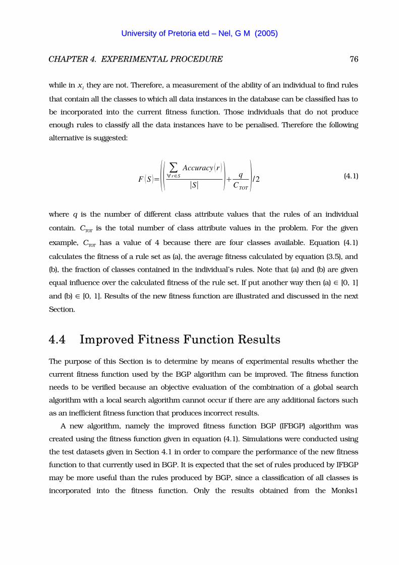
CHAPTER 4. EXPERIMENTAL PROCEDURE 76
while in x1 they are not. Therefore, a measurement of the ability of an individual to find rules
that contain all the classes to which all data instances in the database can be classified has to
be incorporated into the current fitness function. Those individuals that do not produce
enough rules to classify all the data instances have to be penalised. Therefore the following
alternative is suggested:
F �S ���� � rS
Accuracy �r �
�S� �� qCTOT
� 2 (4.1)
where q is the number of different class attribute values that the rules of an individual
contain. CTOT is the total number of class attribute values in the problem. For the given
example, CTOT has a value of 4 because there are four classes available. Equation (4.1)
calculates the fitness of a rule set as (a), the average fitness calculated by equation (3.5), and
(b), the fraction of classes contained in the individual’s rules. Note that (a) and (b) are given
equal influence over the calculated fitness of the rule set. If put another way then (a) [0, 1]
and (b) [0, 1]. Results of the new fitness function are illustrated and discussed in the next
Section.
4.4 Improved Fitness Function Results
The purpose of this Section is to determine by means of experimental results whether the
current fitness function used by the BGP algorithm can be improved. The fitness function
needs to be verified because an objective evaluation of the combination of a global search
algorithm with a local search algorithm cannot occur if there are any additional factors such
as an inefficient fitness function that produces incorrect results.
A new algorithm, namely the improved fitness function BGP (IFBGP) algorithm was
created using the fitness function given in equation (4.1). Simulations were conducted using
the test datasets given in Section 4.1 in order to compare the performance of the new fitness
function to that currently used in BGP. It is expected that the set of rules produced by IFBGP
may be more useful than the rules produced by BGP, since a classification of all classes is
incorporated into the fitness function. Only the results obtained from the Monks1
UUnniivveerrssiittyy ooff PPrreettoorriiaa eettdd –– NNeell,, GG MM ((22000055))
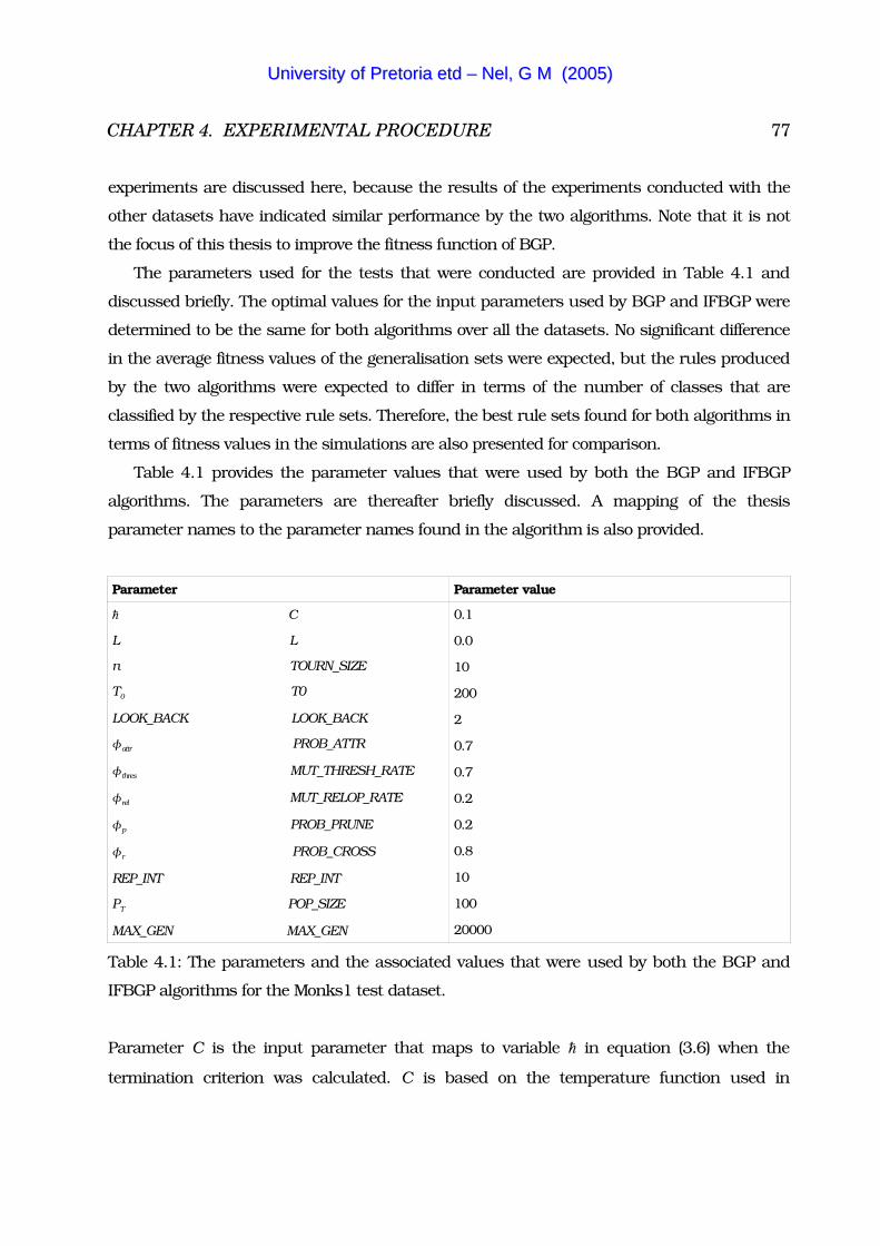
CHAPTER 4. EXPERIMENTAL PROCEDURE 77
experiments are discussed here, because the results of the experiments conducted with the
other datasets have indicated similar performance by the two algorithms. Note that it is not
the focus of this thesis to improve the fitness function of BGP.
The parameters used for the tests that were conducted are provided in Table 4.1 and
discussed briefly. The optimal values for the input parameters used by BGP and IFBGP were
determined to be the same for both algorithms over all the datasets. No significant difference
in the average fitness values of the generalisation sets were expected, but the rules produced
by the two algorithms were expected to differ in terms of the number of classes that are
classified by the respective rule sets. Therefore, the best rule sets found for both algorithms in
terms of fitness values in the simulations are also presented for comparison.
Table 4.1 provides the parameter values that were used by both the BGP and IFBGP
algorithms. The parameters are thereafter briefly discussed. A mapping of the thesis
parameter names to the parameter names found in the algorithm is also provided.
Parameter Parameter value
� C
L L
n TOURN_SIZE
T0 T0
LOOK_BACK LOOK_BACK
�attr PROB_ATTR
�thres MUT_THRESH_RATE
�rel MUT_RELOP_RATE
�p PROB_PRUNE
�r PROB_CROSS
REP_INT REP_INT
PT POP_SIZE
MAX_GEN MAX_GEN
0.1
0.0
10
200
2
0.7
0.7
0.2
0.2
0.8
10
100
20000
Table 4.1: The parameters and the associated values that were used by both the BGP and
IFBGP algorithms for the Monks1 test dataset.
Parameter C is the input parameter that maps to variable � in equation (3.6) when the
termination criterion was calculated. C is based on the temperature function used in
UUnniivveerrssiittyy ooff PPrreettoorriiaa eettdd –– NNeell,, GG MM ((22000055))
CHAPTER 4. EXPERIMENTAL PROCEDURE 78
simulated annealing. Parameter L is the variable in equation (3.7), which was used as a
criterion to add a conditional function to the population of individuals. By manipulating the
parameter L, both a variation in complexity of the produced decision trees, and a variation in
the fitness values of the final population were achieved. The parameter TOURN_SIZE maps to
n in Section 3.2.8 and was used when performing tournament selection by randomly
selecting TOURN_SIZE individuals for the sub-population in order to compare fitness with one
another. Tournament selection was used by both the BGP and IFBGP algorithms and is
described in Section 3.2.8. Parameter T0 maps to T0 that were used in equation (3.6). T0
represents the initial temperature that guarantees that the algorithms will terminate in T0
generations. The LOOK_BACK parameter is used to indicate the size of a queue used to store
previous best decision trees that had been found. By setting the LOOK_BACK parameter to a
large value, the rate of fitness improvement was determined more accurately than for smaller
LOOK_BACK values. The rate of fitness improvement was used to determine whether the tree
complexity must be increased by raising the value of parameter L.
The PROB_ATTR (�attr ), MUT_THRESH_RATE (�thres ), and the MUT_RELOP_RATE (�rel )
parameters were used to indicate, respectively, the probabilities to mutate the attribute
values, the threshold values, and the relational operators in the function expressions held in
the root and internal nodes of the expression trees. The PROB_PRUNE parameter was used to
indicate the probability with which the expression trees were pruned. Parameter
PROB_CROSS (�r ) indicates the probability at which recombination occurred in the
population of the algorithms. Parameter POP_SIZE maps to PT and was used to set the size of
the population that the algorithms maintained during all generation iterations. The
MAX_GEN parameter is a safety parameter that forced the algorithms to terminate if the
simulated annealing algorithm failed. Parameter MAX_GEN was never used since parameter
T0 terminated as indicated in all tests performed.
Thirty simulations were performed for each test data for both the algorithms. The mean
fitness values were then calculated for each generation in the simulations. Graphs were
drawn from the values that were calculated for each generation indicating the average fitness
values as a function of the generations. However, the number, typically more than 100 and
up to 2000 generations, made the task of interpreting the graphs impossible. Any
improvements that IFBGP had were very difficult to interpret with so many generations to
UUnniivveerrssiittyy ooff PPrreettoorriiaa eettdd –– NNeell,, GG MM ((22000055))
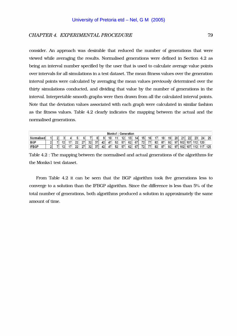
CHAPTER 4. EXPERIMENTAL PROCEDURE 79
consider. An approach was desirable that reduced the number of generations that were
viewed while averaging the results. Normalised generations were defined in Section 4.2 as
being an interval number specified by the user that is used to calculate average value points
over intervals for all simulations in a test dataset. The mean fitness values over the generation
interval points were calculated by averaging the mean values previously determined over the
thirty simulations conducted, and dividing that value by the number of generations in the
interval. Interpretable smooth graphs were then drawn from all the calculated interval points.
Note that the deviation values associated with each graph were calculated in similar fashion
as the fitness values. Table 4.2 clearly indicates the mapping between the actual and the
normalised generations.
Table 4.2 : The mapping between the normalised and actual generations of the algorithms for
the Monks1 test dataset.
From Table 4.2 it can be seen that the BGP algorithm took five generations less to
converge to a solution than the IFBGP algorithm. Since the difference is less than 5� of the
total number of generations, both algorithms produced a solution in approximately the same
amount of time.
UUnniivveerrssiittyy ooff PPrreettoorriiaa eettdd –– NNeell,, GG MM ((22000055))
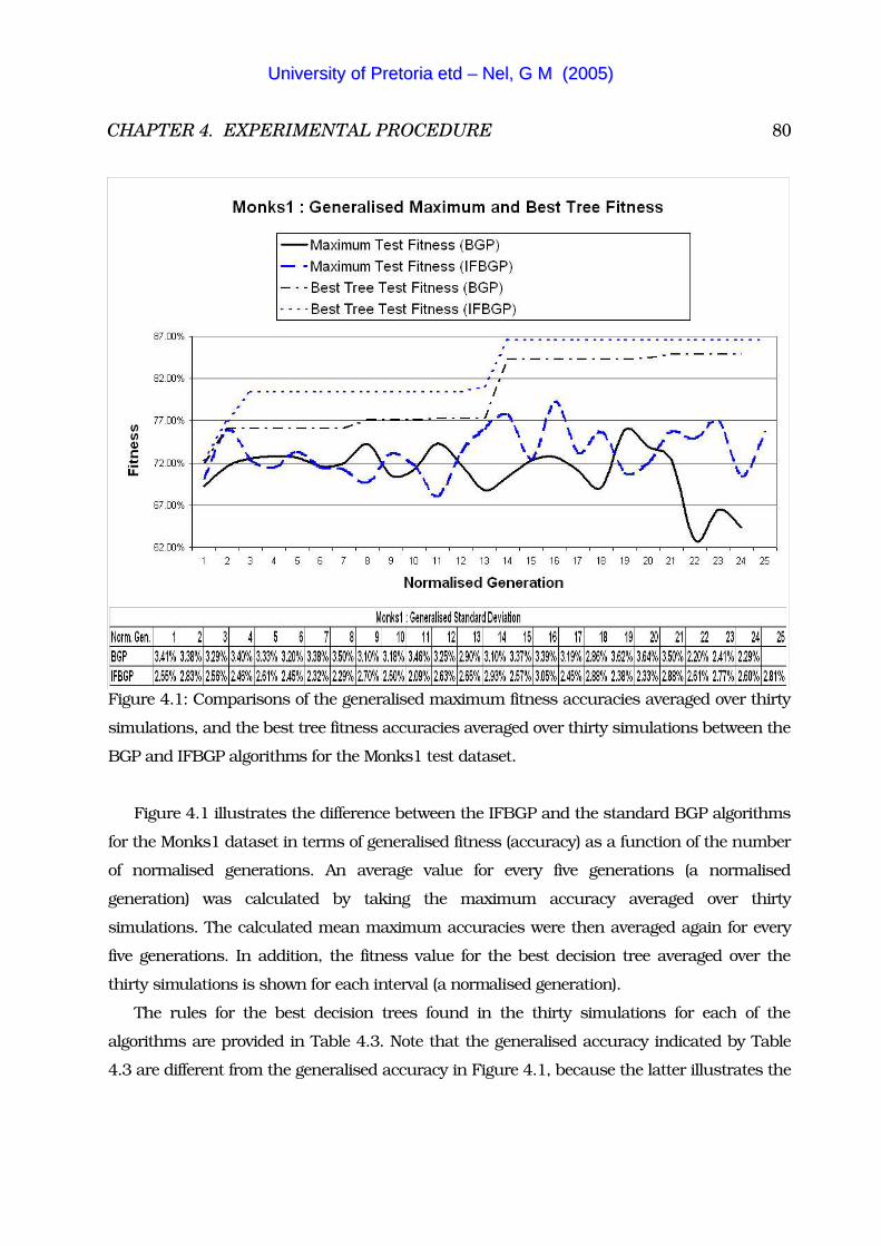
CHAPTER 4. EXPERIMENTAL PROCEDURE 80
Figure 4.1: Comparisons of the generalised maximum fitness accuracies averaged over thirty
simulations, and the best tree fitness accuracies averaged over thirty simulations between the
BGP and IFBGP algorithms for the Monks1 test dataset.
Figure 4.1 illustrates the difference between the IFBGP and the standard BGP algorithms
for the Monks1 dataset in terms of generalised fitness (accuracy) as a function of the number
of normalised generations. An average value for every five generations (a normalised
generation) was calculated by taking the maximum accuracy averaged over thirty
simulations. The calculated mean maximum accuracies were then averaged again for every
five generations. In addition, the fitness value for the best decision tree averaged over the
thirty simulations is shown for each interval (a normalised generation).
The rules for the best decision trees found in the thirty simulations for each of the
algorithms are provided in Table 4.3. Note that the generalised accuracy indicated by Table
4.3 are different from the generalised accuracy in Figure 4.1, because the latter illustrates the
UUnniivveerrssiittyy ooff PPrreettoorriiaa eettdd –– NNeell,, GG MM ((22000055))
CHAPTER 4. EXPERIMENTAL PROCEDURE 81
mean best tree accuracy over thirty simulations, while Table 4.3 illustrates the extracted rules
of the best tree found in the thirty simulations.
From the results, the following observations were made for both the BGP and IFBGP
algorithms: The graphs in Figure 4.1 illustrates that the maximum generalised fitness
averaged over 30 simulations continually oscillated in fitness value as the members of the
population were subjected to the evolutionary operators, namely, mutation, recombination,
pruning and selection. Figure 4.1 also indicates that sudden increases in fitness values
occurred for the average best decision tree found over 30 simulations, for both algorithms.
The sudden increases in fitness values occurred because once the evolutionary operators
were applied, then new regions of the search space were discovered, resulting in an
improvement in the fitness of the average best tree found. The improvements to the average
best tree fitness values are clearly visible at normalised generation intervals 1 to 3, and 13 to
14 for both algorithms.
The maximum generalised fitness accuracy that was averaged over 30 simulations, is a
measure that indicates how well the algorithms generalised the test data. From Figure 4.1 it
is clear that the IFBGP algorithm outperformed the BGP algorithm. The highest mean fitness
value obtained by IFBGP was 79� at normalised generation interval 16, which was 3� better
than the highest mean maximum fitness of 76� that BGP obtained at normalised generation
interval 19. IFBGP produced more accurate trees for the simulations that were performed,
which was also supported by the associated average standard deviation results.
UUnniivveerrssiittyy ooff PPrreettoorriiaa eettdd –– NNeell,, GG MM ((22000055))
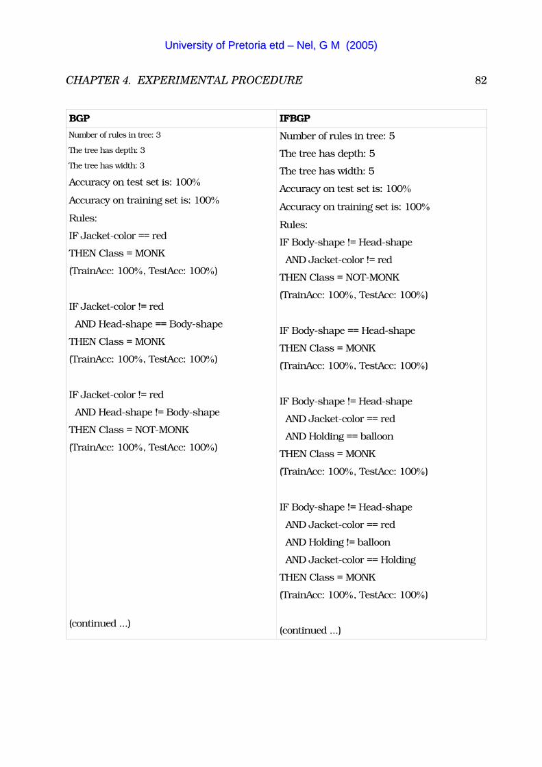
CHAPTER 4. EXPERIMENTAL PROCEDURE 82
BGP IFBGPNumber of rules in tree: 3
The tree has depth: 3
The tree has width: 3
Accuracy on test set is: 100�
Accuracy on training set is: 100�
Rules:
IF Jacket-color == red
THEN Class = MONK
(TrainAcc: 100�, TestAcc: 100�)
IF Jacket-color != red
AND Head-shape == Body-shape
THEN Class = MONK
(TrainAcc: 100�, TestAcc: 100�)
IF Jacket-color != red
AND Head-shape != Body-shape
THEN Class = NOT-MONK
(TrainAcc: 100�, TestAcc: 100�)
(continued ...)
Number of rules in tree: 5
The tree has depth: 5
The tree has width: 5
Accuracy on test set is: 100�
Accuracy on training set is: 100�
Rules:
IF Body-shape != Head-shape
AND Jacket-color != red
THEN Class = NOT-MONK
(TrainAcc: 100�, TestAcc: 100�)
IF Body-shape == Head-shape
THEN Class = MONK
(TrainAcc: 100�, TestAcc: 100�)
IF Body-shape != Head-shape
AND Jacket-color == red
AND Holding == balloon
THEN Class = MONK
(TrainAcc: 100�, TestAcc: 100�)
IF Body-shape != Head-shape
AND Jacket-color == red
AND Holding != balloon
AND Jacket-color == Holding
THEN Class = MONK
(TrainAcc: 100�, TestAcc: 100�)
(continued ...)
UUnniivveerrssiittyy ooff PPrreettoorriiaa eettdd –– NNeell,, GG MM ((22000055))
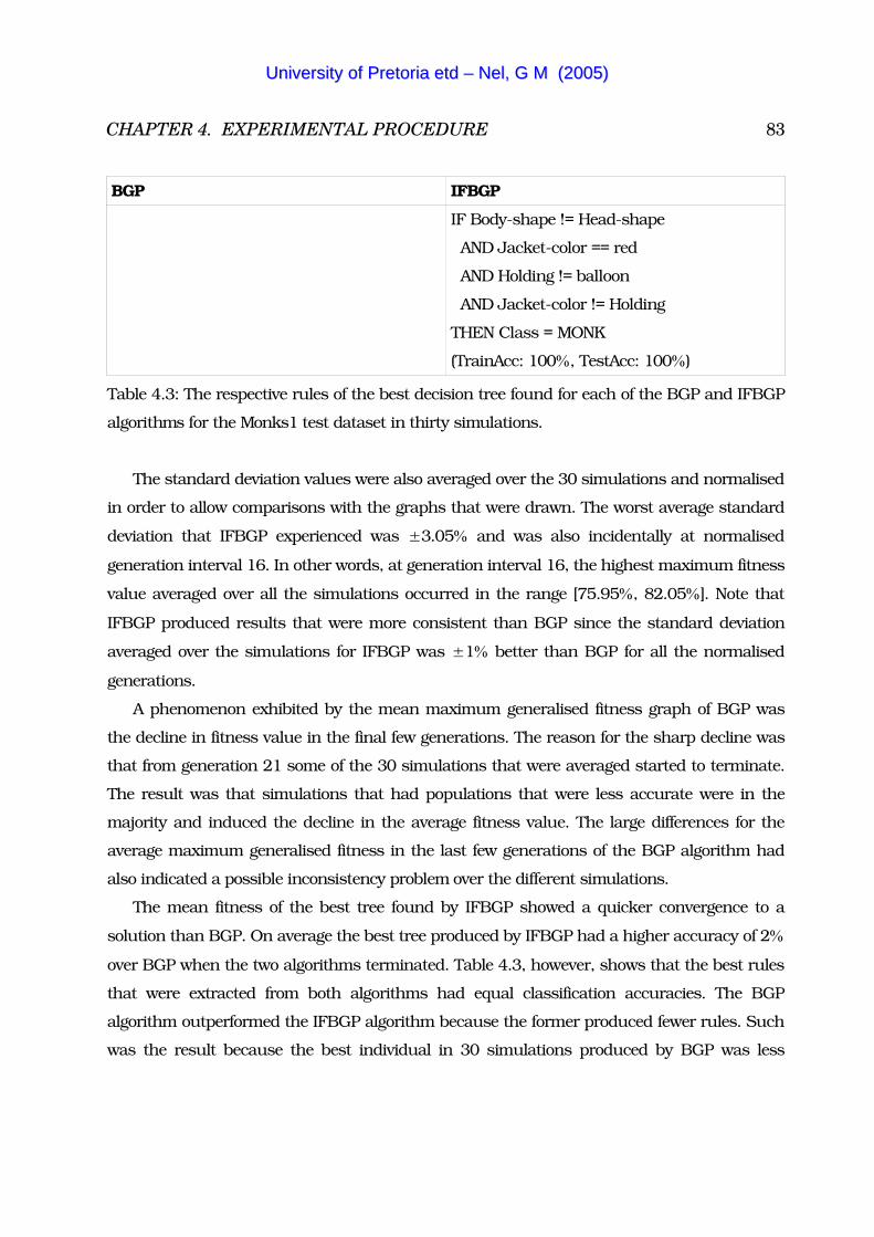
CHAPTER 4. EXPERIMENTAL PROCEDURE 83
BGP IFBGP
IF Body-shape != Head-shape
AND Jacket-color == red
AND Holding != balloon
AND Jacket-color != Holding
THEN Class = MONK
(TrainAcc: 100�, TestAcc: 100�)
Table 4.3: The respective rules of the best decision tree found for each of the BGP and IFBGP
algorithms for the Monks1 test dataset in thirty simulations.
The standard deviation values were also averaged over the 30 simulations and normalised
in order to allow comparisons with the graphs that were drawn. The worst average standard
deviation that IFBGP experienced was �3.05� and was also incidentally at normalised
generation interval 16. In other words, at generation interval 16, the highest maximum fitness
value averaged over all the simulations occurred in the range [75.95�, 82.05�]. Note that
IFBGP produced results that were more consistent than BGP since the standard deviation
averaged over the simulations for IFBGP was �1� better than BGP for all the normalised
generations.
A phenomenon exhibited by the mean maximum generalised fitness graph of BGP was
the decline in fitness value in the final few generations. The reason for the sharp decline was
that from generation 21 some of the 30 simulations that were averaged started to terminate.
The result was that simulations that had populations that were less accurate were in the
majority and induced the decline in the average fitness value. The large differences for the
average maximum generalised fitness in the last few generations of the BGP algorithm had
also indicated a possible inconsistency problem over the different simulations.
The mean fitness of the best tree found by IFBGP showed a quicker convergence to a
solution than BGP. On average the best tree produced by IFBGP had a higher accuracy of 2�
over BGP when the two algorithms terminated. Table 4.3, however, shows that the best rules
that were extracted from both algorithms had equal classification accuracies. The BGP
algorithm outperformed the IFBGP algorithm because the former produced fewer rules. Such
was the result because the best individual in 30 simulations produced by BGP was less
UUnniivveerrssiittyy ooff PPrreettoorriiaa eettdd –– NNeell,, GG MM ((22000055))
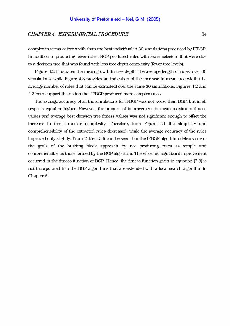
CHAPTER 4. EXPERIMENTAL PROCEDURE 84
complex in terms of tree width than the best individual in 30 simulations produced by IFBGP.
In addition to producing fewer rules, BGP produced rules with fewer selectors that were due
to a decision tree that was found with less tree depth complexity (fewer tree levels).
Figure 4.2 illustrates the mean growth in tree depth (the average length of rules) over 30
simulations, while Figure 4.3 provides an indication of the increase in mean tree width (the
average number of rules that can be extracted) over the same 30 simulations. Figures 4.2 and
4.3 both support the notion that IFBGP produced more complex trees.
The average accuracy of all the simulations for IFBGP was not worse than BGP, but in all
respects equal or higher. However, the amount of improvement in mean maximum fitness
values and average best decision tree fitness values was not significant enough to offset the
increase in tree structure complexity. Therefore, from Figure 4.1 the simplicity and
comprehensibility of the extracted rules decreased, while the average accuracy of the rules
improved only slightly. From Table 4.3 it can be seen that the IFBGP algorithm defeats one of
the goals of the building block approach by not producing rules as simple and
comprehensible as those formed by the BGP algorithm. Therefore, no significant improvement
occurred in the fitness function of BGP. Hence, the fitness function given in equation (3.8) is
not incorporated into the BGP algorithms that are extended with a local search algorithm in
Chapter 6.
UUnniivveerrssiittyy ooff PPrreettoorriiaa eettdd –– NNeell,, GG MM ((22000055))
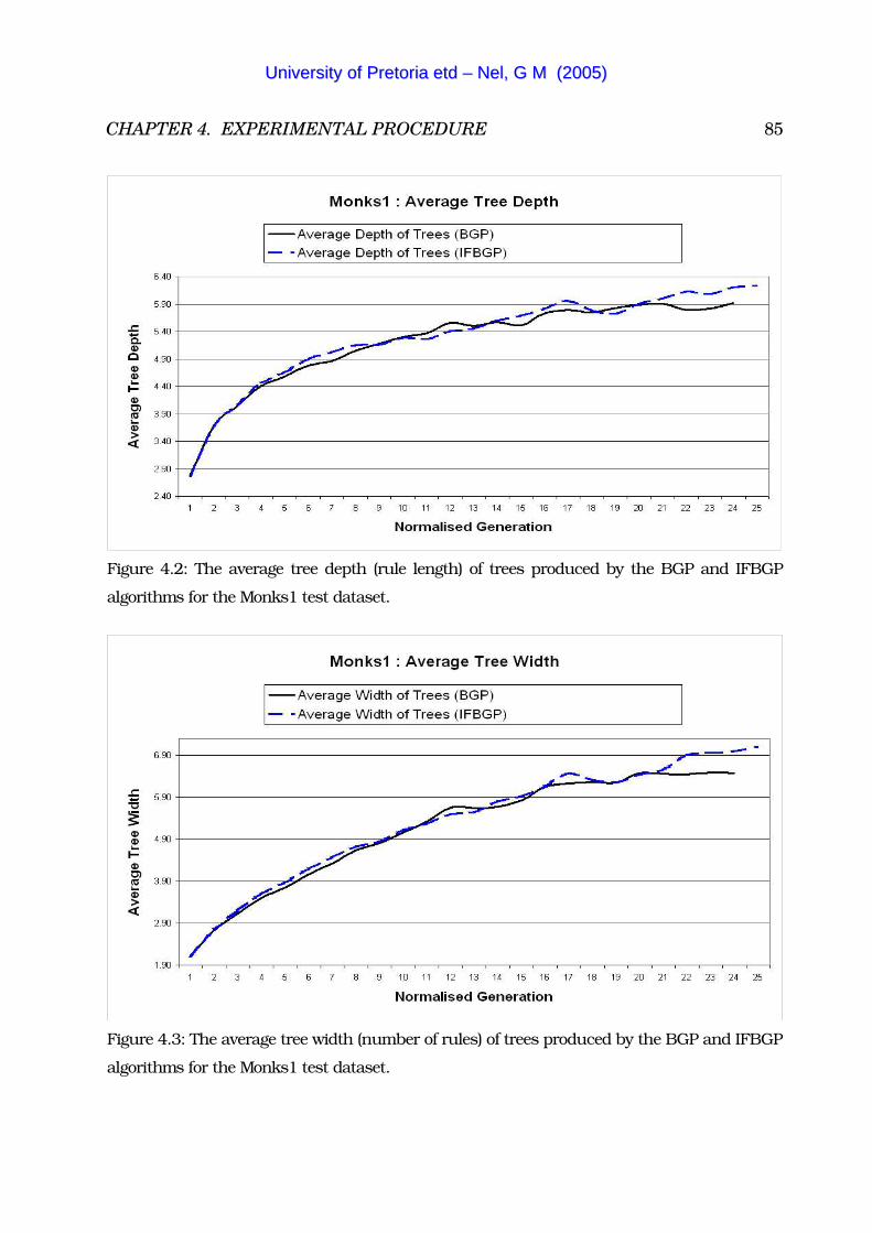
CHAPTER 4. EXPERIMENTAL PROCEDURE 85
Figure 4.2: The average tree depth (rule length) of trees produced by the BGP and IFBGP
algorithms for the Monks1 test dataset.
Figure 4.3: The average tree width (number of rules) of trees produced by the BGP and IFBGP
algorithms for the Monks1 test dataset.
UUnniivveerrssiittyy ooff PPrreettoorriiaa eettdd –– NNeell,, GG MM ((22000055))

CHAPTER 4. EXPERIMENTAL PROCEDURE 86
4.5 Concluding Remarks
This Chapter described the test databases used in all simulations that were performed. The
experimental procedures implemented were also presented. The main objective of this
Chapter was to compare a new fitness function with that used currently by BGP. The main
conclusion was that the current fitness function utilised by the BGP algorithm is adequate for
further use by BGP and any newly developed algorithms in subsequent experiments. The
next Chapter provides a background overview of local search methods as well as the specific
method that is to be combined with the BGP algorithm.
UUnniivveerrssiittyy ooff PPrreettoorriiaa eettdd –– NNeell,, GG MM ((22000055))
Chapter 5
Local Search Methods�������������� ������������� �������� ������������ ���� ������������� �������������� ��
�������� ���� ������������� ������� ����������� ���� ���������������� ����������� ����� ����
�������������� ���������� ���� �������������������� ���������� �������������������������� ���� ���
��������� ������������������������������ �����
�������������������������� ����������������� �� ����� ���� ����� ��������� ��������������
���� ������������ ��������������� ���� ���� ����������������� ���� ����� � ������������������������
������������� �������������� � �������!������������� ��������� �� ������ ���� ����� � ������
������������������������ ����� ������������������ �� ������ ���� ���� ��������� ��� ������������
"������� ���������������������������� �� ������ ���� ��������������������������������������
��������������� ��������������������� ��������� ���� ������������� ��� �������������������������
���� ����������������������� ���������#��� ������������������� �������� ���� ������������
5.1 Local Search Algorithms
The goal of evolutionary algorithms is either to generate a maximum quality solution, or to
find a solution of sufficient quality in the minimum amount of time. The goal of an
optimisation algorithm is to assign values to the variables of a problem such that an objective
function is maximised or minimised. Local search methods are usually deterministic
algorithms specialising in finding solutions of maximum quality (local solutions). Several
examples of local search algorithms [79, 31, 6, 7, 49, 35, 20, 61, 1, 29] can be found in the
literature. Local search methods can also be used for refining (optimising) arbitrary points in a
87
UUnniivveerrssiittyy ooff PPrreettoorriiaa eettdd –– NNeell,, GG MM ((22000055))
CHAPTER 5. LOCAL SEARCH METHODS 88
search space into better quality solutions. The arbitrary points are the ‘coarse’ solutions
provided by other evolutionary methods, known as global search algorithms that specialise in
finding solutions of sufficient quality in the minimum amount of time.
On the other hand, global search algorithms such as genetic algorithms, evolutionary
strategies and evolutionary programming can be thought of as probabilistic search
techniques inspired by the principles of natural evolution. Global search algorithms are best
suited to generating approximate solutions to problems quickly (faster than local search
algorithms). However, global search algorithms are then slower to refine the solution than
local search algorithms. The reason that solutions found by global search are said to be
approximations is because global search often makes large ‘jumps’ in the search space in
order to sift through it efficiently. Therefore, only very few global search algorithms can
guarantee good accuracy in the solution found by each of them.
In contrast, local search algorithms use domain-specific knowledge and are often
employed as local search operators in order to accelerate the convergence of global search
algorithms (specifically EAs) on complex and difficult problem spaces [9]. Domain-specific
knowledge is required for local search operators because they are usually representation-
specific. With local search operators being representation-specific, it is meant that the local
search operators depend upon the choice made to represent possible solutions (individuals in
an EA population). Typically, local search incorporates a significant amount of representation
and problem-specific knowledge. In fact, the most decisive step on which nearly all successes
or failures of the local search approach depends, is making the proper selection for
representing the possible solutions to any local search problem. Due to the dependency of the
local search operators on the representation of the solutions, local search algorithms do not
generalise well for different optimisation problems. In order to obtain a valid representation
(formulation) of the local search problem, the following three requirements, as given by
Moscato [57], have to be satisfied, and valid mathematical encodings for possible solutions
have to be given.
Assume the input domain set IP of problem P can be characterised by a set of instances
x � IP . A set of corresponding answers ansP(x) can be established for a search space SP or
each instance x, with the following three properties. The first is that each element s � SP
represents an answer, ansP(x). The symbol s(x) is defined as the subset s(x) � ansP(x),
UUnniivveerrssiittyy ooff PPrreettoorriiaa eettdd –– NNeell,, GG MM ((22000055))
CHAPTER 5. LOCAL SEARCH METHODS 89
which identifies the feasible (also known as acceptable or valid) solutions to problem P.
Therefore, the second property is that when working with decision (‘Yes-No’) problems, at
least one element of s(x) stands for a ‘Yes’ answer and is represented by one element in SP.
The third property is that when working with optimisation problems, at least one optimal
element y* of s(x) is represented by one element in SP . Note that the first property refers to
ansP(x) and not to s(x).
The following definitions are given so as to explain the representation of the local search
problem, because the representation of the latter has an enormous influence on how the local
search algorithm moves between neighbouring solutions in the search space. The
neighbourhood of the search space SP , for a given problem P and the instance x � IP , is given
in the form of N(s,x). In most implementations of local search algorithms, the elements of
N(s,x) are referred to as the set of possible moves that define transitions between
neighbouring solutions. In other words, the set N(s,x), also known as the neighbouring
solutions, is the assignment of each element s � SP where N(s,x) � SP . Therefore, it is clear
that each member s’ � N(s,x) is called a neighbour of s in the neighbourhood of SP .
These types of moves are really the key to local search, because the moves are defined as
‘local modifications’ of some part of SP . Hence the terminology of ‘local’ search that is
assigned to the whole search paradigm now under discussion. It is important to note that
there is no implication that local search is bound to some kind of distance-relationship
between different solutions. In other words, solutions in SP are not required to be within a
certain distance for a transition to be made by local search from one solution to a
neighbouring solution.
The ability given any s � SP to find a sequence of transitions that can reach all other
neighbouring solutions s’ in SP , is known as the ergodicity of moves that can be made for the
representation of solutions in a problem. Note that when choosing the local search method for
use in optimising a problem, the ergodicity is an important factor that must be considered.
The ergodicity of moves that can be made is important since it is different depending on
representation of the solutions to the problem. The final choice of representation for the
solutions in a problem is the one where the ergodicity of moves that can be made is the
lowest. In other words, the representation that is chosen is the one where it is easiest to make
UUnniivveerrssiittyy ooff PPrreettoorriiaa eettdd –– NNeell,, GG MM ((22000055))
CHAPTER 5. LOCAL SEARCH METHODS 90
transitions from current solutions to new solutions.
In order to discuss how a local search algorithm ‘navigates’ a search space, in other
words, makes transitions from current to new solutions, a few definitions are given. An
objective function mP(y,x) is viewed as the minimum ‘price’ or ‘cost’ of solution y given
instance x for problem P. The guiding function Fg is defined as the weighted sum of the value
of the objective function mP(y,x) and the distance to a feasible solution. The distinction
between a feasible solution and an optimal one is that the former adheres to constraints of
the problem, which implies that the solution has a valid mathematical encoding. A feasible
solution can coincide with the optimal solution. An optimal solution can be defined as being
either the local or the global optimal solution. A higher weight is assigned to the distance to a
feasible solution since the latter accounts for the feasibility constraint placed on the problem.
Therefore, preference is given to a solution that is feasible rather than one that is optimal.
Let f be the fitness function and f(s0) the fitness of the initial solution s0 � SP . If f(s1) is
the fitness of the next solution s1 � SP , assume that f(s0) � f(s1) if P is a minimising problem.
A local search algorithm ‘navigates’ a search space by starting at solution s0 � SP . The local
search then uses a transition based on the neighbourhood of the solution, as the algorithm
iterates through the search space to generate a new solution s1. The initial solution s0 can be
constructed in several ways, including the use of a given algorithm (e.g. global search), or
some form of heuristic. A heuristic is a rule or principle that guides the algorithm to the
objective (the solution). The local search algorithm selects the next solution by using both the
objective function and the guiding function. The process explained above is performed
iteratively and is referred to as hill climbing. Hence, hill climbing is used to generate new
solutions that improve on previous ones. Note that not all local search methods, e.g. neural
network training [38, 43], perform hill climbing.
Other local optimisation search methods are now discussed in short to review the variety
that is available in the literature. In general, local optimisation algorithms terminate if no
further improvement is found for the fitness function associated with the algorithm, or if the
fitness of the solution found is sufficient according to a user specified value, or when the
maximum number of search operations is exceeded.
In Birru et al. [6], two local optimisation search methods are used, namely the conjugate
gradient (Press et al., 1992), and the Solis and Wets (Solis and Wets, 1981) methods. The
UUnniivveerrssiittyy ooff PPrreettoorriiaa eettdd –– NNeell,, GG MM ((22000055))
CHAPTER 5. LOCAL SEARCH METHODS 91
conjugate gradient method performs line searches on a one-dimensional slice of a function,
specified by a search direction. Therefore, the conjugate gradient method requires
computation of the first order derivatives in order to obtain gradient information. The Solis
and Wets method does not require derivative information since normally distributed steps are
used to generate new points in search space. Adding zero mean deviates to the current point
generates a new point. If the fitness function value of the new point is worse than that of the
current point, the algorithm takes a step in the opposite direction. The fitness function value
of the newly generated point in the opposite direction is now compared with the current
point’s fitness function value. If neither of the generated points’ fitness function values
improve on the current point, then for the next iteration a new random point is generated,
and its fitness function value compared with the current point.
In Liang et al. [49], a Landscape Approximation with Local Search (LALS) algorithm is
used to change indirectly the roughness of the fitness landscape. The indirect change to the
roughness of the fitness landscape is accomplished by applying a quadratic approximation on
a parent individual in order to estimate the approximate location of the next offspring. The
new offspring is kept if the fitness function value improved.
Parallel local search as explained in [57] can be achieved by using more than one
optimisation algorithm when performing local search. The use of multiple optimisers can be
accomplished by separating the optimisation algorithms into independent threads of
execution. To facilitate multiple optimisation algorithms, the local search space of the global
solution can be decomposed into the representations required by each individual local
optimisation algorithm. Each local optimisation algorithm then tries to improve the quality of
the global solution. As an additional benefit the parallel local search method enables the use
of a multi-processing environment. Techniques that utilise population-based approaches are
prime candidates for such parallel local search techniques and concurrent processing. The
distribution of the processes among separate processors also contributes to better
performance. However, note that the processes must still interact with each other in order to
improve significantly the performance of the search algorithm. Generally speaking, both
parallel hill climbing and memetic algorithms can make use of multiple optimisation
algorithms.
Simulated annealing (SA) is another local search algorithm used for combinatorial
problems, and/or is used to perform approximate optimisation of large search spaces [1, 29].
UUnniivveerrssiittyy ooff PPrreettoorriiaa eettdd –– NNeell,, GG MM ((22000055))
CHAPTER 5. LOCAL SEARCH METHODS 92
Generally, the SA algorithm is used for problems where the derivatives are not available for
the objective function that is optimised. The minimisation of the objective function is viewed
by the SA algorithm as being equivalent to a physical system, such as the annealing (cooling)
process of metal. To reach an equilibrium state, the SA algorithm repeatedly accepts or rejects
the change from state i to state j according to probability P. Two parameters are used to
control the SA algorithm, namely, the temperature T, and L that represents the number of
state changes that are allowed per temperature change. An acceptance of a state-transition
from state i to j is based on the probability,
P �i� j ���e� f �i � f � j �
T �if f � j � f �i �
1 if f � j �� f �i � (5.1)
After an initial state was generated, the criterion in equation (5.1) is used to consider
accepting or rejecting L state transitions. A repetitive procedure is followed whereby the
temperature T is reduced according to a cooling schedule. With each new temperature the
criterion in equation (5.1) is considered L times. Near-optimal solutions can be obtained by
determining experimentally the appropriate values for T, L and the cooling schedule.
The local search methods discussed above had all been used as optimisers in conjunction
with global search algorithms. The next Section discusses in depth the combination of local
with global search techniques.
5.2 Combining Local and Global Search
The goal of this Section is to motivate the combination of a local search method with a global
search algorithm, for example BGP. The combination of global and local search has proved to
be more effective in finding the best quality solution in the shortest period of time rather than
global search alone [57, 79, 31, 77, 6, 7, 49, 35]. The global algorithm is extended with local
search in order to combine the advantages of the local and global search methodologies.
Global search advantages include generality, robustness and global search efficiency. By
generality is meant that the algorithm can be applied to a very large set of optimisation
problems and still be able to produce solutions that are comparable to other known methods
UUnniivveerrssiittyy ooff PPrreettoorriiaa eettdd –– NNeell,, GG MM ((22000055))

CHAPTER 5. LOCAL SEARCH METHODS 93
used to solve the problems. By robustness is meant that the algorithm produces a good
solution even though the data contain noise. Robustness also means that the algorithm
repeatedly produces good solutions with small fault variances for the same problem, even
though different initialisation conditions are used. Global search efficiency implies that the
algorithm can find a global solution of sufficient quality in a short period of time. The global
solution may even be the best possible solution that can be found. However, few global search
algorithms can guarantee that the solution that each of them had found cannot be further
improved. Global search (such as EAs) achieve search efficiency by searching large portions of
the complete search space at the same time.
Local search methods have an advantage in that when a local neighbourhood (localised
portion) of the search space is searched, the local solution found is optimal with a very high
accuracy. In order for local search to find a local solution with high accuracy, small
modifications are made to the solution, which means that small steps are taken through the
local neighbourhood. The small search steps that are taken contribute to longer search times,
unless the local search algorithm starts its search in the general vicinity of the optimal
solution.
Cotta [20] discourages the use of local search algorithms for large search space
landscapes that are convoluted and rough. A convoluted and rough landscape in the context
of a search space means that the search space has many possible solutions to the problem
(refer to Figure 2.1). In other words, local search methods are appropriate only for optimising
small localised portions of the search space, and not for optimising the complete search
space. This local search constraint is due to the inability of local search to continue with a
search once local minima or maxima were found. Clearly, global search methods such as EAs
can efficiently search convoluted and rough landscapes better than local search because of
their evolutionary search approach. Consequently, once an appropriate solution is found by
global search, local search can then be used to improve the accuracy of the solution. Several
examples of the combination of local and global search algorithms can be found in the
literature [79, 31, 6, 7, 49, 35, 13]. The references illustrate not only effective local search
algorithms, but also techniques for combining local search methods with global search
algorithms. The methods for combining local search with global search are as follow:
� Embedded: a local search algorithm can be embedded as an operand in a global search
algorithm. Chellapilla et al. [6, 7] reported on experimentations done on five well-known
UUnniivveerrssiittyy ooff PPrreettoorriiaa eettdd –– NNeell,, GG MM ((22000055))

CHAPTER 5. LOCAL SEARCH METHODS 94
optimisation problems. Two local search methods, conjugate gradient and Solis and Wets,
were each in turn embedded as an operand of an evolutionary programming algorithm
(EP). Two EP algorithms, namely classical evolutionary programming (CEP) and fast
evolutionary programming (FEP) were used in the simulations. The new EP algorithms
consistently produced solutions that were as good as, or better than those produced by the
EP algorithms without a local search operand.
� Parallel: both local and global search are used in turn during the execution of the main
algorithm to search for solutions until a termination condition is achieved. At first, global
search is used exclusively to find the promising regions in the search space. Then the local
search method is given the opportunity to spend progressively more time on refining the
solutions found by global search. As a consequence global search has progressively less
time to search the complete search space [79].
� Serial: a method of combining global and local search that introduces less complexity to
the global search algorithm. A solution is first found with the global search algorithm. The
global algorithm is not interrupted and it searches exclusively for a solution until a
termination condition is achieved. Then the solution found by the global search algorithm
is used as input to the local search algorithm.
Whichever approach is used to combine global and local search, the common idea is to
exploit the advantages provided by both search paradigms. Memetic algorithms are the class
of local and global search combination where the local search algorithm is embedded as an
operand in the global search algorithm. The following Section provides a discussion with
regards to memetic algorithms and presents a general framework.
UUnniivveerrssiittyy ooff PPrreettoorriiaa eettdd –– NNeell,, GG MM ((22000055))
CHAPTER 5. LOCAL SEARCH METHODS 95
5.3 Memetic Algorithms
In the previous Sections global and local search were reviewed and the combination of the two
paradigms discussed. Chapter 2 provided background of the processes of optimisation and
classification, and the notion of memetic algorithms (MA) was introduced. A review of the MA
framework as given by [57] is now given. The reason for reviewing the MA framework is that
an indication is given of the appropriate places in which to embed a local search method in a
global search algorithm such as EAs. Examples of implemented MAs can be found in the
literature and include [35, 61, 65, 44, 54].
5.3.1 Local-Search-based Memetic Algorithm
In general, problems that have been shown to be NP-hard can be solved approximately by
local search based memetic algorithms (LS-based MAs) [57]. The pseudo-code framework for
the algorithm structure of a LS-based MA as given by [57] is provided in Figure 5.1. Assume
that the global search method used in Figure 5.1 is a GA.
The meaning of the terms as they appear in the algorithm is provided in this and the
following subsections. Concurrent with the explanation of the terms, an example is provided
to illustrate the functionality and give better insight into the ‘Local-Search-Engine’ algorithm.
The Travelling Salesman Problem (TSP) is a well-known NP-hard problem that is well
understood in the artificial intelligence community, and for that reason is used in the
example. Assume that search space SP exists for problem P, and any feasible solution found
for P is given by s(x) � SP . Let the objective function mP(y,x) for P map every feasible solution
y � s(x) to a numerical value. Note that the solution s(x) � SP with regards to the TSP
example is known as a tour.
UUnniivveerrssiittyy ooff PPrreettoorriiaa eettdd –– NNeell,, GG MM ((22000055))
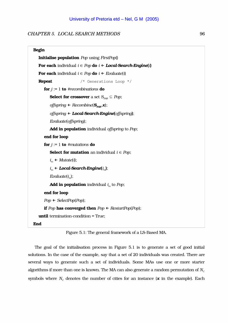
CHAPTER 5. LOCAL SEARCH METHODS 96
Begin
Initialise population Pop using FirstPop()
For each individual i � Pop do i Local-Search-Engine(i)
For each individual i � Pop do i Evaluate(i)
Repeat /* Generations Loop */
for j := 1 to #recombinations do
Select for crossover a set SPAR � Pop;
offspring Recombine(SPAR,x);
offspring Local-Search-Engine(offspring);
Evaluate(offspring);
Add in population individual offspring to Pop;
end for loop
for j := 1 to #mutations do
Select for mutation an individual i � Pop;
im Mutate(i);
im Local-Search-Engine(im);
Evaluate(im);
Add in population individual im to Pop;
end for loop
Pop SelectPop(Pop);
if Pop has converged then Pop RestartPop(Pop);
until termination-condition = True;
End
Figure 5.1: The general framework of a LS-Based MA.
The goal of the initialisation process in Figure 5.1 is to generate a set of good initial
solutions. In the case of the example, say that a set of 20 individuals was created. There are
several ways to generate such a set of individuals. Some MAs use one or more starter
algorithms if more than one is known. The MA can also generate a random permutation of NC
symbols where NC denotes the number of cities for an instance (x in the example). Each
UUnniivveerrssiittyy ooff PPrreettoorriiaa eettdd –– NNeell,, GG MM ((22000055))
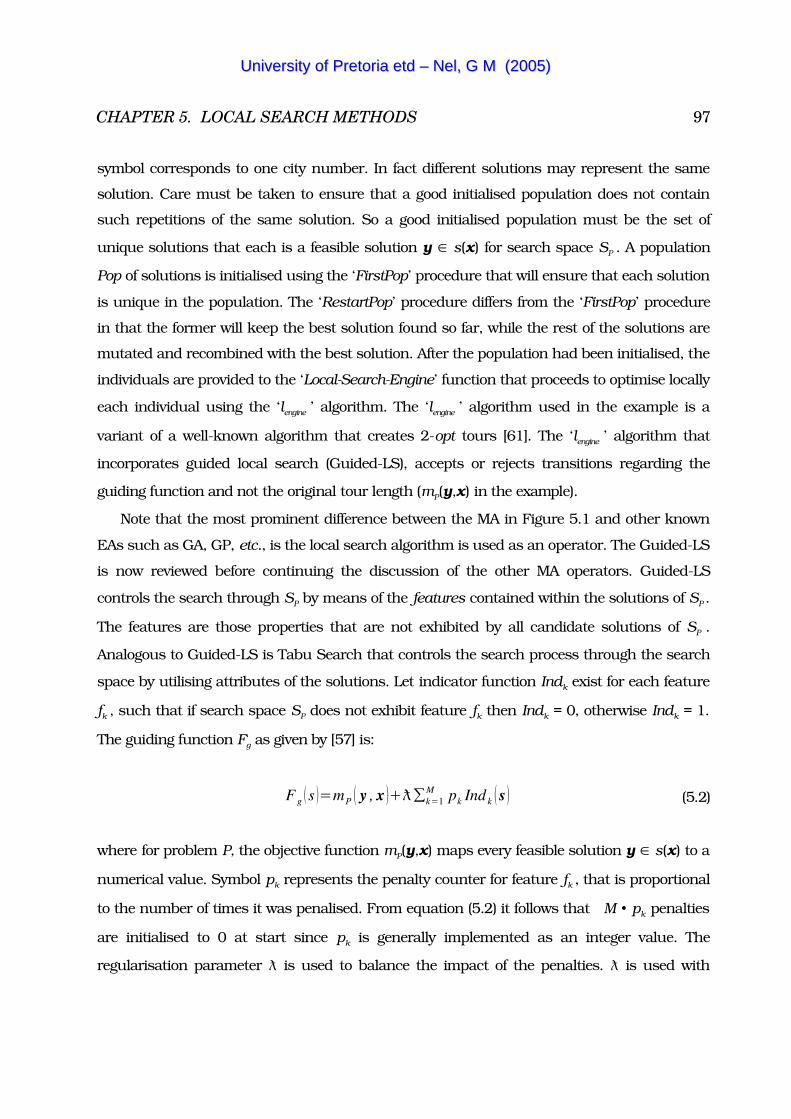
CHAPTER 5. LOCAL SEARCH METHODS 97
symbol corresponds to one city number. In fact different solutions may represent the same
solution. Care must be taken to ensure that a good initialised population does not contain
such repetitions of the same solution. So a good initialised population must be the set of
unique solutions that each is a feasible solution y � s(x) for search space SP . A population
Pop of solutions is initialised using the ‘FirstPop’ procedure that will ensure that each solution
is unique in the population. The ‘RestartPop’ procedure differs from the ‘FirstPop’ procedure
in that the former will keep the best solution found so far, while the rest of the solutions are
mutated and recombined with the best solution. After the population had been initialised, the
individuals are provided to the ‘Local-Search-Engine’ function that proceeds to optimise locally
each individual using the ‘lengine ’ algorithm. The ‘lengine ’ algorithm used in the example is a
variant of a well-known algorithm that creates 2-opt tours [61]. The ‘lengine ’ algorithm that
incorporates guided local search (Guided-LS), accepts or rejects transitions regarding the
guiding function and not the original tour length (mP(y,x) in the example).
Note that the most prominent difference between the MA in Figure 5.1 and other known
EAs such as GA, GP, etc., is the local search algorithm is used as an operator. The Guided-LS
is now reviewed before continuing the discussion of the other MA operators. Guided-LS
controls the search through SP by means of the features contained within the solutions of SP .
The features are those properties that are not exhibited by all candidate solutions of SP .
Analogous to Guided-LS is Tabu Search that controls the search process through the search
space by utilising attributes of the solutions. Let indicator function Indk exist for each feature
fk , such that if search space SP does not exhibit feature fk then Indk = 0, otherwise Indk = 1.
The guiding function Fg as given by [57] is:
F g �s ��mP � y , x ����k�1M pk Ind k � s � (5.2)
where for problem P, the objective function mP(y,x) maps every feasible solution y � s(x) to a
numerical value. Symbol pk represents the penalty counter for feature fk , that is proportional
to the number of times it was penalised. From equation (5.2) it follows that M � pk penalties
are initialised to 0 at start since pk is generally implemented as an integer value. The
regularisation parameter � is used to balance the impact of the penalties. � is used with
UUnniivveerrssiittyy ooff PPrreettoorriiaa eettdd –– NNeell,, GG MM ((22000055))
CHAPTER 5. LOCAL SEARCH METHODS 98
respect to the original objective function (in other words the length of the tour). There are
several ways to choose the value of �, and one such way is [57]:
��0.3�L �initial tour �
N c
(5.3)
where NC is the number of cities and L(initial tour) is the length of the tour associated with the
specific individual (an individual obtained after the first optimisation phase by using only the
local search method).
For each feature fk a cost value is assigned to help rate its significance relative to other
features. By assigning a cost for each feature, a search that is trapped in a local minimum
can systematically reduce the features that contribute to the current state by penalising
them. Penalisation of the most constantly significant features is also possible. Penalisation is
controlled by using the function utilk(s) that takes into account how many times each feature
has been penalised before. Features that are selected to be penalised are those that maximise
utilk(s) in a minimisation problem. The function as given by [57] is:
utilk � s ��Ind k � s ��cost k
1� pk
(5.4)
The denominator includes protection in case of a zero penalty count. Figure 5.2 presents the
pseudo-code for the Guided-LS as given by [57].
UUnniivveerrssiittyy ooff PPrreettoorriiaa eettdd –– NNeell,, GG MM ((22000055))

CHAPTER 5. LOCAL SEARCH METHODS 99
Procedure (Guided) Local-Search-Engine
Begin
iter�0 ;
for each feature k do pk �0 ;
repeat
F g � s ��mP � y , x ����k�1M pk Ind k � s �
siter�1�lengine �siter , F g �siter � � ;
for each feature k do utilk � s �� Ind k � s ��cost k
1� pk
for each feature k which maximises utilk do pk� pk�1 ;
iter�iter�1 ;
until guided local search termination condition = True;
return the ‘best-so-far’ found solution regarding m p� y , x� ;
Figure 5.2: The (Guided) Local-Search-Engine Algorithm.
Note that it is not necessary to perform the ‘Evaluate’ procedure in Figure 5.1 in order to
evaluate the guiding function Fg until a local optimum has been obtained. The Guided-LS
algorithm terminates when a local solution has been found, or once all the features have been
processed. The individual that has improved the most in terms of the objective function since
the ‘Restart’ procedure was last called, is returned by the procedure.
5.3.2 Recombination
Recombination for EAs was discussed in detail in Sections 2.3.5 and 3.1.2. Recombination is
reviewed only as it was implemented by [57] in the context of the TSP example. The
recombination procedure represented by the ‘Recombine(SPAR,x)’ function in Figure 5.2
creates a single child individual (offspring) by combining at least two valid parent individuals
(two or more tours that are defined as the set SPAR). Selection of individuals for recombination,
UUnniivveerrssiittyy ooff PPrreettoorriiaa eettdd –– NNeell,, GG MM ((22000055))
CHAPTER 5. LOCAL SEARCH METHODS 100
mutation and as members of the next generation was also reviewed in Sections 2.3.7 and
3.1.2. Hence, selection methods are not reviewed here.
Implementation of the recombination procedure can be done in a variety of ways, ranging
from a simple efficient (i.e. Polynomial-time) ‘k-merger’ algorithm [57] to more complex
recombination operators. The newly created individual is then optimised using the local
search method and then either added to or withheld from the general population depending
on the selection criteria.
In the example the recombination procedure involves taking two parent tours that have
edge sets A and B respectively. All edges common to both parents (i.e. A � B) are then
selected to be part of the child. Edges in the (AB) � (BA) set are listed in increasing order
with respect to their lengths, while arbitrarily breaking the ties between edges. When iterating
through the list, a test is performed as to whether an edge can be added to the child while
avoiding the generation of an infeasible tour. Such an infeasible tour is characterised by a
closed cycle with fewer than the total number of cities, or by having a city visited more than
once. In other words the city has three or more edges incident on it. If the testing conditions
are not met, then do not add the edge. If the list is exhausted, and there is still no valid
individual, then proceed with a patching operation. The latter can also be done in a variety of
ways, but, in the example, Moscato resorts to the simpler idea of running the nearest-
neighbour constructive heuristic on the set of cities that have none or only one edge (the so-
called endpoints of the set of sub strings).
When the offspring is added back to the population, a check is performed that there is no
other individual already in the population with the same offspring value. If there is such an
individual with the same offspring value, then the tour to be introduced is altered by
randomly performing a chain of 2-changes.
The convergence rate of the MA can be controlled by the recombination probability
parameter as explained in Section 2.3.5, or with a recombination parameter
(‘#recombinations’ in Figure 5.1) given by [57]. If a recombination parameter is used, then
there are a fixed number of recombinations that will occur during each generation of the
simulation.
UUnniivveerrssiittyy ooff PPrreettoorriiaa eettdd –– NNeell,, GG MM ((22000055))
CHAPTER 5. LOCAL SEARCH METHODS 101
5.3.3 Mutation
Analogue to the ‘Recombine’ function, the ‘Mutate’ function performs an operation whereby a
number of individuals are modified structurally. However, unlike recombination, new genetic
material is introduced. Mutation was discussed in Sections 2.3.6 and 3.1.2.
The mutation operation in Figure 5.1 as provided by [57], is implemented as a random
process based on the same neighbourhood definition implicit to the ‘lengine ’ discussed before.
For the example, one individual is selected from which four edges �ci , ci�1� , �c j , c j�1� ,
�ck , ck�1� and �cm , cm�1� are removed. The edges are then replaced by four new edges
�ci , ck�1� , �c j , cm�1� , �ck , ci�1� , and �cm , c j�1� in order to create another valid tour.
The double-bridge move given by [44, 45] is used for mutation, but replacement by other
methods is also possible. As with the recombination method, the newly created individuals
are locally optimised and tested once that individual has mutated.
One approach other than a random undirected jump for the mutation operator is to
exchange a sequence of facilities until the new individuals have reached a predefined distance
from the original individuals. The term facilities is referred to as memes when speaking in
terms of MAs, or genetic material when speaking in terms of EAs.
Another approach for mutation is the use of a binomial minimal mutation operator. Firstly,
the term minimal mutation is defined. When a parent � has chromosomes Y and X, the Y
chromosome will be the minimal mutation of chromosome X, only if there is no other
chromosome present in parent � that is closer to X than Y is to X with respect to the distance
D between them. The distance measure between two chromosomes is explained in detail in
[65]. According to [65], the set of minimal mutations of X is given by
M D�X ���Y�� � � Z�� � �X � : D �X ,Y ��D �X , Z �� (5.5)
where ‘�’ denotes set subtraction. A single parameter pM is passed to the Binomial Minimal
Mutation (BMM) operator. The pM parameter specifies the probability of performing each
possible minimal mutation.
For the TSP example a chromosome A can be represented as a set of exactly n alleles. The
set of alleles is the set of possible routes the problem might have. Chromosome A is therefore
UUnniivveerrssiittyy ooff PPrreettoorriiaa eettdd –– NNeell,, GG MM ((22000055))
CHAPTER 5. LOCAL SEARCH METHODS 102
the set of all possible edges between cities in the TSP example. Note that chromosome A
represents a tour by the set of undirected edges it contains. From the binomial distribution
B(n,pM), k mutations to perform is selected, where n is the number of alleles in each
chromosome. It is ensured by selection of the case of orthogonal representations that the
BMM behaviour mimics that of conventional gene-wise mutation. A new sequence of k
chromosomes is generated. The first in the sequence is the chromosome that is to be
mutated, while the last in the sequence is the resultant chromosome. Therefore, the k
chromosomes produced are each a minimal mutation of the previous chromosome.
In the example, the ‘SelectPop’ function selects a specified number of the best individuals
by using the cost function only. Therefore, what the selection procedure effectively does is to
reduce the size of the set. Clearly the selection of the subset is not always determined by the
objective or guiding function. In fact, the selection of such a subset may be influenced by
other features of the individuals, such as the interest of maximising some measure of
diversity of the selected set.
The ‘RestartPop’ function is used when the population has converged. A ‘diversity-crisis’
operation is defined as being a measure that indicates whether the whole population has
similar solutions below some threshold. The ‘diversity-crisis’ operation is also used to
determine whether the population has in fact converged. For example, if the ‘incumbent
solution’ (best individual) did not improve for three consecutive generations, then assume
that the Guided-LS procedure will no longer be able to produce better solutions. In the
example provided by [57], the ‘RestartPop’ function was not implemented, but Moscato
provided some hints as to how the function can be implemented. Generally, the best
incumbent solution is kept while the other individuals are mutated or a new population is
created using some random method. The selection of the best individual is a relative measure,
and it generally entails the selection of the individual that has improved the most in terms of
fitness value since the last ‘RestartPop’ function call. The whole population is optimised and
evaluated after the ‘RestartPop’ function call, while the whole process is repeated again until
the termination condition is reached.
5.3.4 Termination Condition
For a termination condition time expiration or generation expiration criteria can be used as
UUnniivveerrssiittyy ooff PPrreettoorriiaa eettdd –– NNeell,, GG MM ((22000055))
CHAPTER 5. LOCAL SEARCH METHODS 103
well as more adaptive procedures as explained in Section 2.1. A more complex combination of
the mentioned termination criteria is also possible. Most often the process is terminated when
no more improvement occurs in the fitness value of the incumbent solution.
With the MA framework review completed, it is now necessary to discuss the local search
method that will be combined with the BGP algorithm.
5.4 Directed Increasing Incremental Local Search
Directed Increasing Incremental Local Search (DIILS) is a variation of the hill climbing local
search method that was specifically developed for this thesis by the author. DIILS was
developed for application specifically in combination with the BGP algorithm discussed in
Chapter 3. Therefore, DIILS is explained in the context of BGP.
Directed searches with increasing incremental steps are performed on the all the nodes of
those decision trees (individuals) that were selected, rather than performing small random
changes on them. Once an individual was locally optimised, it not a requirement to optimise
the individual again if only a sub-tree in the individual's tree structure is replaced. Only the
top node (root) of the new sub-tree is given as a parameter to the local search method.
Therefore, only the sub-tree is locally optimised. Hence, computational complexity is reduced
by not locally optimising a complete decision tree every time it is chosen for local optimisation.
The particular local search method is best explained by an example. The root node of a
decision or expression tree is a function as described by the tuple given in equation (3.1), with
the root and internal nodes each representing a selection from the function set. For the
following example assume that the threshold of a function is a real number. If the threshold is
a continuous value, then the accuracy associated with that threshold is used to determine
the incremental value with which the threshold value is incremented. Note that the precision
associated with each attribute’s value is a given input provided for the standard BGP
algorithm and is therefore available for use by the DIILS method.
Assume that a decision tree produced by a global search algorithm contained the following
rule: ‘IF a9 � 19, then CLASS A’. Remember that the internal nodes of a decision tree contain
the antecedent of the rule format given in equation (2.1), such as the example relational
function (condition) ‘a9 � 19’. The attribute ‘a9’ and its associated value ‘19’, known as the
threshold, are the arguments of the ‘�’ relational operator. The leaf node of the decision tree is
UUnniivveerrssiittyy ooff PPrreettoorriiaa eettdd –– NNeell,, GG MM ((22000055))
CHAPTER 5. LOCAL SEARCH METHODS 104
a class attribute value that is the consequence of the rule format given in equation (2.1).
Figure 5.3 is used to illustrate the relationship between the threshold value and fitness
function value for the given example rule extracted from a decision tree. In other words, for
the given rule a change in the threshold of the relational function will vary the number of data
instances correctly classified by the rule, which means a change in the fitness value of the
rule. Figure 5.3 is also used to provide a visual guide to the steps involved when performing a
directed local search of an attribute and the associated attribute value.
In Figure 5.3, the associated attribute value of ‘a9’ is optimised; therefore the initial
starting point is the real number 19. Real number 25 is the objective that must be found
which represents the correct value that produces the best fitness value for the relational
condition. When the search on the threshold value starts, no search direction is initially
known. A random decision is therefore made to decrement the threshold with a value of 1.
Step 1 shows the new threshold in the random direction with lower value. The new threshold
value is 18 that indicates that the associated fitness value had decreased. Since the fitness
value has decreased, the threshold value is reset to 19 and the search is directed in the
opposite direction with the increment value still set to 1. For the step 2, the threshold value
for the condition is increased to 20, which results in a better fitness value than the condition
with threshold value 19. The direction of search has now been determined and a directed
incremental search can continue. Every time the algorithm establishes a direction the
incremental value is reset to 1. The resulting new threshold value is 21, and again represents
an improvement in fitness as is shown in step 3.
UUnniivveerrssiittyy ooff PPrreettoorriiaa eettdd –– NNeell,, GG MM ((22000055))
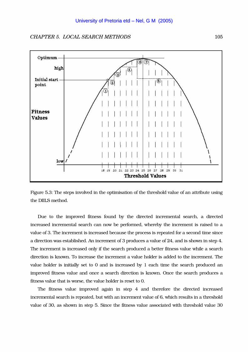
CHAPTER 5. LOCAL SEARCH METHODS 105
Figure 5.3: The steps involved in the optimisation of the threshold value of an attribute using
the DIILS method.
Due to the improved fitness found by the directed incremental search, a directed
increased incremental search can now be performed, whereby the increment is raised to a
value of 3. The increment is increased because the process is repeated for a second time since
a direction was established. An increment of 3 produces a value of 24, and is shown in step 4.
The increment is increased only if the search produced a better fitness value while a search
direction is known. To increase the increment a value holder is added to the increment. The
value holder is initially set to 0 and is increased by 1 each time the search produced an
improved fitness value and once a search direction is known. Once the search produces a
fitness value that is worse, the value holder is reset to 0.
The fitness value improved again in step 4 and therefore the directed increased
incremental search is repeated, but with an increment value of 6, which results in a threshold
value of 30, as shown in step 5. Since the fitness value associated with threshold value 30
UUnniivveerrssiittyy ooff PPrreettoorriiaa eettdd –– NNeell,, GG MM ((22000055))
CHAPTER 5. LOCAL SEARCH METHODS 106
decreased, the search reverts back to the previous threshold value of 24, and the increment
size is reset to 1. Note that the increment is again undirected. An increment value of 1 is used
again and the value holder is reset to 0 since the search process has restarted. The
momentum of the direction to search in is considered and dictates that a greater value than
the current one must be selected, so the resulting threshold value of 25 is produced and is
shown in step 6. The fitness value again improved; therefore a direction to search in has been
established. The increment is set again to 1, because it is the first time since the restart of the
search that direction has been assigned. The value holder which was 0 is added to the
increment. The value holder is then incremented by 1. The new threshold value shown in step
7 is 26 and is greater than the previous threshold value of 25. The new fitness value
associated with the threshold value 26 is lower, and because the increment was 1 and the
search direction was known, the search reverts back to the previous threshold value of 25
and terminates the search method. Therefore, the termination condition for DIILS is that if
the fitness value of the new associated threshold value decreases and a direction to search in
is known and the incremental value is 1, then terminate the method.
5.5 Concluding Remarks
This Chapter discussed local search methods. Three methods for combining local search and
global search algorithms were then presented in order to familiarise the reader with the
concepts. The MA framework was then reviewed with a given example. From the MA
framework it became apparent that an MA is an EA that embeds local search as an operand.
The DIILS method was then introduced and discussed with an example in the context of
BGP.
In the next Chapter, the BGP algorithm is combined with the DIILS method. Specifically,
the DIILS method is implemented as an operator within the original BGP algorithm to create a
new MA. An additional algorithm is also created whereby the BGP algorithm is combined in a
simple fashion with the DIILS method. As a result, any significant differences between the
simple combination of global and local search algorithms and a MA are reported on. All
results obtained from the simulations are compared with the original BGP algorithm. The
results are then used to draw conclusions regarding the MA and the combined global-local
search algorithm.
UUnniivveerrssiittyy ooff PPrreettoorriiaa eettdd –– NNeell,, GG MM ((22000055))
Chapter 6
Extending BGP for Rule Extraction������������ �������������������������������������� ����������������������������������� �!�������
����� ���������������"�������#��$�!������������������������� ����� ������������
� �����%���������� ��� ������������ ������������������������"���������� �����! ��! ��������
� �������������������������� ���������������&��!�'�� ����� ����� � �� ����$����������$���
���� �� ����� ��� � ��� �� !�� ���������"� ��� ������ ����� !��� � ���%��� � �� ����� �� !��� �
������ � � ������ #"� ��� ���%�� ��� �� ��� � ������ ��� �� ����%��� �� !�� ����� � ������ ���
� �� �� � �� �����$� �� �� �� ����� ���� ��������"� ���%���� � ��%��� ��� ���$���� � �� ���� �� �
�������$��%��������� �������������������� ����!��� ��������"�
6.1 Extending the BGP Algorithm
A short introduction is presented in the next Section to define properly and discern the
algorithms proposed with which to extend the standard BGP algorithm. Each extended
algorithm is discussed and reasons are provided for the specific extension. The expected
increase in computational complexity of each of the extended algorithms over the standard
BGP algorithm is then reviewed. Some important questions are raised concerning the
extension of the standard BGP algorithm, which will be answered in Section 6.2. In Section
6.2.1, the experimental results produced by the extended algorithms and the standard BGP
algorithm are illustrated, compared and discussed. Section 6.2.2 draws some conclusions
regarding the extended algorithms. Section 6.3 presents some final remarks.
107
UUnniivveerrssiittyy ooff PPrreettoorriiaa eettdd –– NNeell,, GG MM ((22000055))
CHAPTER 6. EXTENTED BGP FOR RULE EXTRACTION 108
6.1.1 Introduction
The standard BGP algorithm is a global search algorithm used for the extraction of symbolic
rules from datasets. One approach to improve the accuracy of rules extracted by BGP is to
perform local search at the appropriate time. Motivation for the combination of local and
global search was provided in Chapter 5, and therefore is not repeated here.
When combining local and global search algorithms, the local search method typically
used is a hill-climbing algorithm. The latter performs repeated incremental local mutations of
the rules contained within an individual, e.g. threshold values, operators and attributes.
Local search is performed until no further improvement in fitness can be found for that
individual. The local search method (DIILS) that is used to extend the BGP algorithm was
presented in Section 5.4. Two possible strategies are explored for extending the standard BGP
algorithm with a local search algorithm. In the first strategy local search is used to refine the
solution found by the standard BGP algorithm, and is therefore tentatively referred to as the
‘Enhanced Building Block Approach to Genetic Programming’ (EBGP) algorithm. For the
second strategy local search is combined as an operand in the standard BGP algorithm, to
create the tentatively named ‘Memetic Building Block Approach to Genetic Programming’
(MBGP) algorithm. Hence, the EBGP algorithm refines only the solution provided by the
standard BGP algorithm, while MBGP actively refines all possible solutions produced by the
initial random selection process, as well those solutions obtained during the evolutionary
process. The difference is explained between the EBGP and MBGP algorithms, because in the
literature the two approaches are sometimes confused and not clearly distinguished. Hence,
each subsection that explains the local search extension to BGP includes a pseudo-algorithm
that clearly illustrates the place where the local search algorithm is incorporated into the
standard BGP global search algorithm. Clearly, the local search algorithm extensions will
influence the associated computational complexity of the extended BGP algorithm as
compared to the standard BGP algorithm. Therefore, computational complexity is explicitly
reviewed as an additional Section following the discussions regarding the extended
algorithms.
6.1.2 Enhanced Building Block Approach to Genetic Programming
In the first strategy to combine local and global search, the standard BGP algorithm is allowed
UUnniivveerrssiittyy ooff PPrreettoorriiaa eettdd –– NNeell,, GG MM ((22000055))

CHAPTER 6. EXTENTED BGP FOR RULE EXTRACTION 109
to produce, in a normal fashion, the solution with the best accuracy that it can find. After the
BGP algorithm finds the best solution, the DIILS local search algorithm is used to refine and
further optimise the solution. Note that the strategy discussed does not influence the BGP
algorithm directly, but rather offers a possible accuracy refinement of the produced solution.
Performance is expected to be relatively the same as that of the original BGP algorithm,
because local search is performed as an additional step before the algorithm invokes the final
post-processing rule extraction operation and terminates. It is important to stress that in the
strategy explained here, local search optimisation of the solutions is not performed during the
life cycle of the global search algorithm, hence the strategy is only considered as an
‘enhancement’ in this thesis. The strategy is therefore appropriately named the ‘Enhanced
Building Block Approach to Genetic Programming’ (EBGP) algorithm.
After completion, the EBGP algorithm exits with a locally optimised decision tree that is
hopefully more accurate than that found by the original BGP algorithm alone. Figure 6.1
illustrates the EBGP algorithm in pseudo-code.
6.1.3 Memetic Building Block Approach to Genetic Programming
The second strategy employed is to incorporate the local search algorithm as an operand of
the global search algorithm that is used. The motivation for the inclusion of a local search
operation during the global search process is provided by the criticism of the Building Block
Hypothesis (BBH) for Genetic Programming as provided by O'Reilly [62]. The criticism was
reviewed in Section 3.2.2, and is only mentioned here. One of the fundamental problems
noted by [62] is that the BBH, in other words the BGP algorithm, cannot provide a guarantee
that the building blocks used to construct the individuals in a population are optimal. O'Reilly
explains that the volatility and random search that occur over the lifetimes of the individuals
in a generation contribute to building blocks that can not be guaranteed to be optimal. The
building blocks used in individuals in a population of the BGP algorithm are only assumed to
be optimal.
UUnniivveerrssiittyy ooff PPrreettoorriiaa eettdd –– NNeell,, GG MM ((22000055))
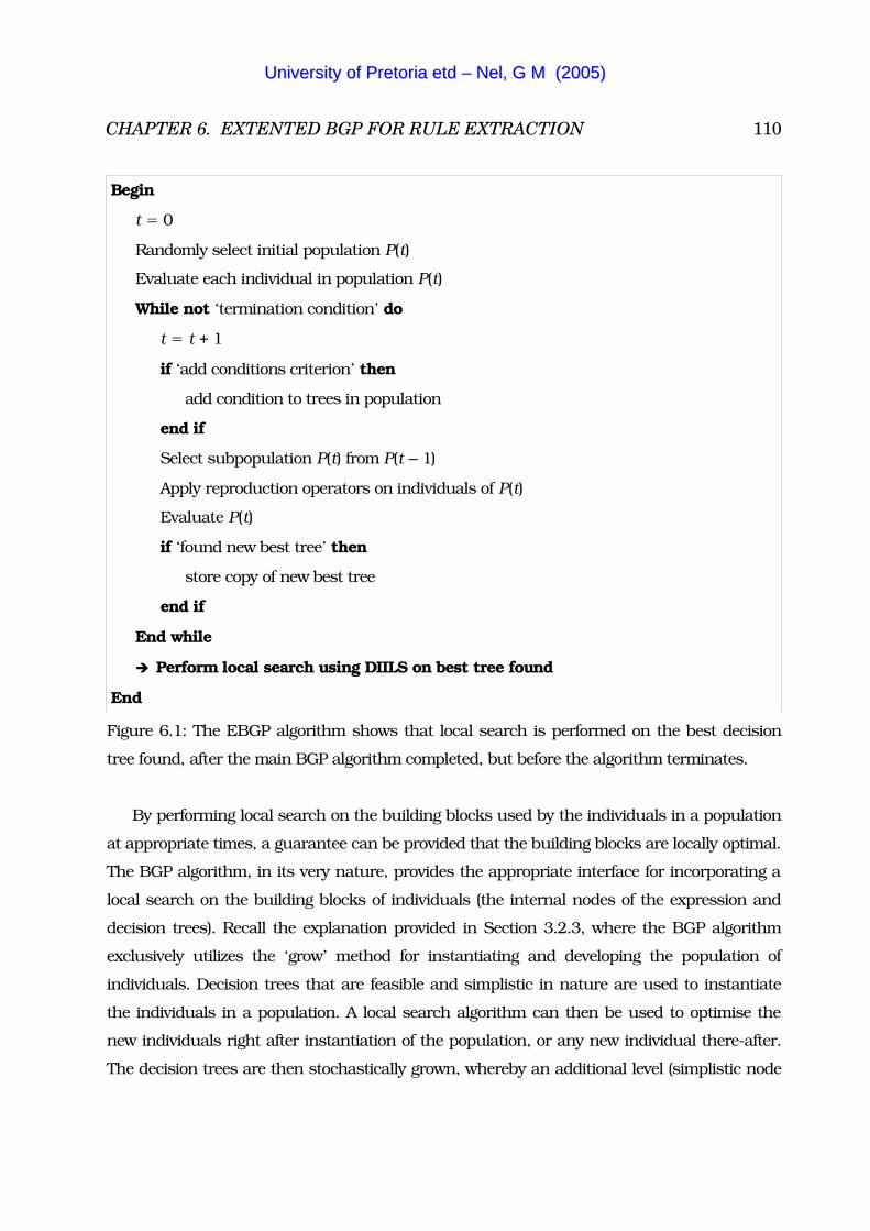
CHAPTER 6. EXTENTED BGP FOR RULE EXTRACTION 110
Begin
t � 0
Randomly select initial population P(t)
Evaluate each individual in population P(t)
While not ‘termination condition’ do
t � t � 1
if ‘add conditions criterion’ then
add condition to trees in population
end if
Select subpopulation P(t) from P(t � 1)
Apply reproduction operators on individuals of P(t)
Evaluate P(t)
if ‘found new best tree’ then
store copy of new best tree
end if
End while
� Perform local search using DIILS on best tree found
End
Figure 6.1: The EBGP algorithm shows that local search is performed on the best decision
tree found, after the main BGP algorithm completed, but before the algorithm terminates.
By performing local search on the building blocks used by the individuals in a population
at appropriate times, a guarantee can be provided that the building blocks are locally optimal.
The BGP algorithm, in its very nature, provides the appropriate interface for incorporating a
local search on the building blocks of individuals (the internal nodes of the expression and
decision trees). Recall the explanation provided in Section 3.2.3, where the BGP algorithm
exclusively utilizes the ‘grow’ method for instantiating and developing the population of
individuals. Decision trees that are feasible and simplistic in nature are used to instantiate
the individuals in a population. A local search algorithm can then be used to optimise the
new individuals right after instantiation of the population, or any new individual there-after.
The decision trees are then stochastically grown, whereby an additional level (simplistic node
UUnniivveerrssiittyy ooff PPrreettoorriiaa eettdd –– NNeell,, GG MM ((22000055))
CHAPTER 6. EXTENTED BGP FOR RULE EXTRACTION 111
with leaves known as sub-trees) is added to the terminal nodes of the initial population
members. Right after a choice in the standard BGP algorithm is made to perform the ‘grow’,
recombination (crossover), or mutation operations on individuals, local search can be
performed on the changed individuals. Note that because local search on the internal nodes is
performed since the start of the algorithm, only the latest level added during the last ‘grow’
phase requires optimisation by the local search algorithm. For those individuals that were
selected for crossover or mutation, only those portions of the new or existing individuals that
were modified need to be optimised by the local search algorithm.
By performing a local search on the decision trees before they are grown, the extended
BGP algorithm can now guarantee that the most locally optimal building blocks are used
within the individuals. Therefore, the concern expressed by O'Reilly regarding unfit building
blocks is addressed. Due to the incorporation of a local search algorithm as an operand
within the standard BGP global search algorithm, the term ‘Memetic’ is added to the BGP
acronym to produce the name that is used - Memetic Building Block Approach to Genetic
Programming (MBGP).
A further explanation is required to address the question of what happens to an individual
that is mutated during the execution of the newly defined MBGP algorithm. No guarantee can
be provided concerning the fitness of any mutated individual’s building blocks unless they are
also locally optimised before the individual is introduced back and can compete with the rest
of the population. Hence, when a probabilistic decision is made to mutate an individual
(decision tree), a stochastic choice for the internal node is made, to be replaced by a new
randomly produced sub-tree. Clearly the unchanged nodes of the individual do not require
optimisation if the tree was previously optimised. Only the replacement sub-tree requires to
be optimised locally within the context of the current individual.
The reproductive operation used, namely recombination (crossover) as explained in
Section 3.2, also introduces variety to the population with some randomness associated with
the operation. Therefore, the produced offspring is also locally optimised by the local search
method that optimises the exchanged sub-trees in the context of the newly created and
recombined individuals.
The termination condition for the local search algorithm operand is simple in that local
search is applied to an individual, until the fitness of the individual does not improve any
further. Figure 6.2 illustrates in pseudo-code the inclusion of the local search method as an
UUnniivveerrssiittyy ooff PPrreettoorriiaa eettdd –– NNeell,, GG MM ((22000055))
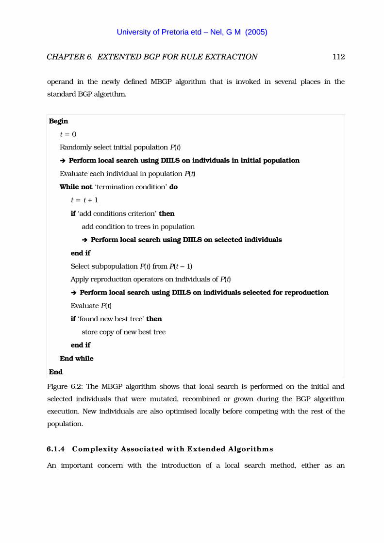
CHAPTER 6. EXTENTED BGP FOR RULE EXTRACTION 112
operand in the newly defined MBGP algorithm that is invoked in several places in the
standard BGP algorithm.
Begin
t � 0
Randomly select initial population P(t)
� Perform local search using DIILS on individuals in initial population
Evaluate each individual in population P(t)
While not ‘termination condition’ do
t � t � 1
if ‘add conditions criterion’ then
add condition to trees in population
� Perform local search using DIILS on selected individuals
end if
Select subpopulation P(t) from P(t � 1)
Apply reproduction operators on individuals of P(t)
� Perform local search using DIILS on individuals selected for reproduction
Evaluate P(t)
if ‘found new best tree’ then
store copy of new best tree
end if
End while
End
Figure 6.2: The MBGP algorithm shows that local search is performed on the initial and
selected individuals that were mutated, recombined or grown during the BGP algorithm
execution. New individuals are also optimised locally before competing with the rest of the
population.
6.1.4 Complexity Associated with Extended Algorithms
An important concern with the introduction of a local search method, either as an
UUnniivveerrssiittyy ooff PPrreettoorriiaa eettdd –– NNeell,, GG MM ((22000055))
CHAPTER 6. EXTENTED BGP FOR RULE EXTRACTION 113
enhancement or as an operand, is the associated increase in computational complexity.
Performance in terms of computation time of the modified BGP algorithm, be it EBGP or
MBGP, may suffer as a direct result of the incorporation of a local search algorithm. With
EBGP local optimisation of the global solution that was found has to occur if the accuracy of
the solution is to be improved. Clearly, EBGP can only perform worse than BGP in terms of
computation complexity, but an improved accuracy of the final solution is possible and may
be worth the additional effort. An important notion is that only the solution found by the BGP
algorithm, hence one decision tree, is locally optimised. Therefore, the additional
computational complexity associated with the EBGP algorithm is relatively low. Experimental
results will attempt to show whether EBGP improved the accuracy of BGP significantly,
thereby offsetting the additional computational complexity.
MBGP will most certainly increase computational complexity, but the algorithm may
converge faster to a solution than the standard BGP algorithm due to the improved internal
building block fitness. An additional benefit of MBGP is that because a local search algorithm
is built into MBGP as an operand that optimises the building blocks of all individuals, a
better-localised accuracy is the result for all solutions produced over every generation. MBGP
is therefore expected to have better problem-resolving properties and higher average fitness
values for the population.
The local optimisation of the initial individuals in the first generation is the most
concerning aspect of the MBGP algorithm. This concern is very real because of the huge
computational complexity involved with the optimisation of all the population members. The
more members a population has, the more initial computational effort is required when
initialising the population. However, remember that the ‘grow’ method is used to build
individuals with the building block approach; hence the initial individuals are all simplistic in
structure, which inherently reduces the effort to compute optimal decision trees. Local search
could be performed with a certain probability in order to reduce the complexity. The problem
with optimising locally only a subset of the population is that the building blocks of the
remaining individuals are not guaranteed to be locally optimal. To simplify the investigation
presented here, the decision was made to optimise locally each individual in the first
generation.
Local search is not required on all members of the population during the rest of the
algorithm execution. Only those individuals selected for expansion (grown), mutation, or
UUnniivveerrssiittyy ooff PPrreettoorriiaa eettdd –– NNeell,, GG MM ((22000055))
CHAPTER 6. EXTENTED BGP FOR RULE EXTRACTION 114
combined in the crossover operation, are subjected to the local search algorithm, and only
that portion of the individual (the decision tree) not yet locally optimised.
6.1.5 Questions Raised by Extending the BGP Algorithm
The theme of this Chapter and the thesis, is to present to the reader two methods for
extending the BGP global search algorithm with a local search algorithm. The resulting
questions from the introduction of the extensions are as follow:
� Are decision trees possible with better or equivalent fitness values in terms of the criteria
specified in Section 2.4.3, using the new extended algorithms, as compared with the
standard BGP algorithm?
� Will the MBGP algorithm converge to a more accurate solution faster than the standard
BGP algorithm?
� If local search algorithms combined with global search algorithms produce solutions with
better accuracy, is there a difference in performance between the MBGP algorithm and the
EBGP algorithm in terms of accuracy, convergence rate and complexity?
The following Section presents the results obtained from experiments performed in order to
answer the above questions.
6.2 Experimental Results
Experimental results were obtained by performing tests on the six different test datasets as
provided by the UCI machine learning repository [8], on the standard BGP, EBGP and MBGP
algorithms. The choice of the six datasets was the same as those used by Rouwhorst [68]. The
results were compared only to standard BGP and not to other RE methods such as C4.5 and
CN2, because BGP was already weighed against these methods [68, 69]. The CN2 and C4.5
algorithms performed on average better than BGP in terms of classification accuracy and time
complexity. However, BGP produced less rules than both CN2 and C4.5.
In order to measure the performance of the extended algorithms (EBGP and MBGP)
compared to that of the standard BGP algorithm, it was decided that the parameters must be
chosen the same (synchronised) during all simulations performed on all the algorithms.
Hence, simulations were first conducted to determine the best parameter settings on the
standard BGP algorithm, which receives no further elaboration here. The best parameter
UUnniivveerrssiittyy ooff PPrreettoorriiaa eettdd –– NNeell,, GG MM ((22000055))
CHAPTER 6. EXTENTED BGP FOR RULE EXTRACTION 115
means that parameters were found which produced the most accurate rules in the shortest
possible time, that best describes the test datasets. The parameters used with each of the
experiments are given as part of the discussion regarding every experiment, but are not
discussed further since Section 4.4 explained all parameters in detail. The result of choosing
the same parameters for all algorithms is that the simulations performed on the extended
algorithms will reflect the direct performance improvements brought on by the combination of
the DIILS algorithm with the standard BGP algorithm. Note that the additional influence of
variations in parameter settings of the extended algorithms are not measured in this thesis
since the goal is to determine the direct value added by combining a local search algorithm
with a global search algorithm. Determining the optimal parameter settings for the extended
algorithms is left for future research.
The fitness function applied in the original BGP algorithm [68] also suited the extended
algorithms because a better fitness function could not be found by means of experimentation
in Section 4.4. The simulations performed on each dataset were repeated 30 times in order to
determine an average for the values shown in the Figures. Hence, a post-processing operation
was performed to determine for each performance measure the mean value of each
generation over the simulations performed. The mean value of each generation over the
simulations was used to create initial graphs. However, the figures were not easily
interpretable due to the number of generations (between 100 and 2000) the algorithms used
to produce solutions. In addition, the fluctuations between generations were rough, which are
less interpretable than smooth graphs. The generations were therefore normalised, i.e., the
actual number of generations used by the algorithms were divided into n discrete intervals
where n is a value specified by the user. For the simulations performed, n was selected to be
25. To obtain the n discrete intervals the actual number of generations are divided by n,
which gives the number of normalised generations, say k, for which a mean value for each of
the measured values are determined, thereby producing interval points. In other words, for
interval k, the average over generations (k � 1)n to kn is calculated and plotted on the given
figures. An interval point is therefore the mean value of a specific performance measure over
k generations such as the average fitness value of the best tree found, or the mean maximum
fitness value. The interval points were then used to produce an interpretable smooth graph.
The mapping of the actual generations to the normalised generations is presented together
with the experimental results.
UUnniivveerrssiittyy ooff PPrreettoorriiaa eettdd –– NNeell,, GG MM ((22000055))
CHAPTER 6. EXTENTED BGP FOR RULE EXTRACTION 116
The experimental results are provided and discussed in the following format for each of
the respective test datasets in Sections 6.2.1 to 6.2.6. The respective test datasets are the
Iono, Iris, Monks1, Monks2, Monks3 and Pima Indians Diabetes test datasets as provided by
[8]. First, a Table is provided with the parameter settings that were used in order to allow the
experiments to be repeated and verified. Note that the parameters are only given and not
discussed, since a proper explanation of each parameter was provided in Section 4.4.
Following the parameter Table is that indicating the mapping between the actual generations
to the normalised generations for the algorithms. A brief discussion is then given regarding
observations made from the normalised generation table.
The graphs illustrating the mean maximum fitness found for each algorithm, as well the
mean fitness of the best decision tree found for the three algorithms are then provided in a
Figure. Note that for the algorithms the mean maximum test fitness was generalised and are
referred to from here on as the mean generalised maximum test fitness. The EBGP and BGP
algorithms are essentially the same algorithm, with a local search being performed by EBGP
on a solution found by BGP. Therefore, it is important to note that the graphs produced will
be the same for most of the generations and are indicated so. Only over the last few
generations will the figures indicate if EBGP was able to improve the BGP solution.
A Table is then presented that provides the rules extracted from the best tree found in the
simulations for each algorithm. This Table is given because it provides supporting evidence
for the graphs in the Figure which shows average values. Note that for each algorithm the
Figure illustrates the graph of the normalised generations versus the fitness of the best tree
found averaged over the 30 simulations, while the Table provides the rules extracted from the
best tree found in the simulations. Hence, the fitness values of the best trees found in the
table are different to the mean fitness values of the best trees as given in the graphs of the
Figure. Finally, the figures indicating tree depth and width, which is a measure to represent
the increase in tree structure complexity, are presented as supporting evidence for the
discussion.
A review of the conclusions that can be drawn from all the results is provided in Section
6.2.7 after all the experimental simulation results were given and discussed in Sections 6.2.1
to 6.2.6.
UUnniivveerrssiittyy ooff PPrreettoorriiaa eettdd –– NNeell,, GG MM ((22000055))
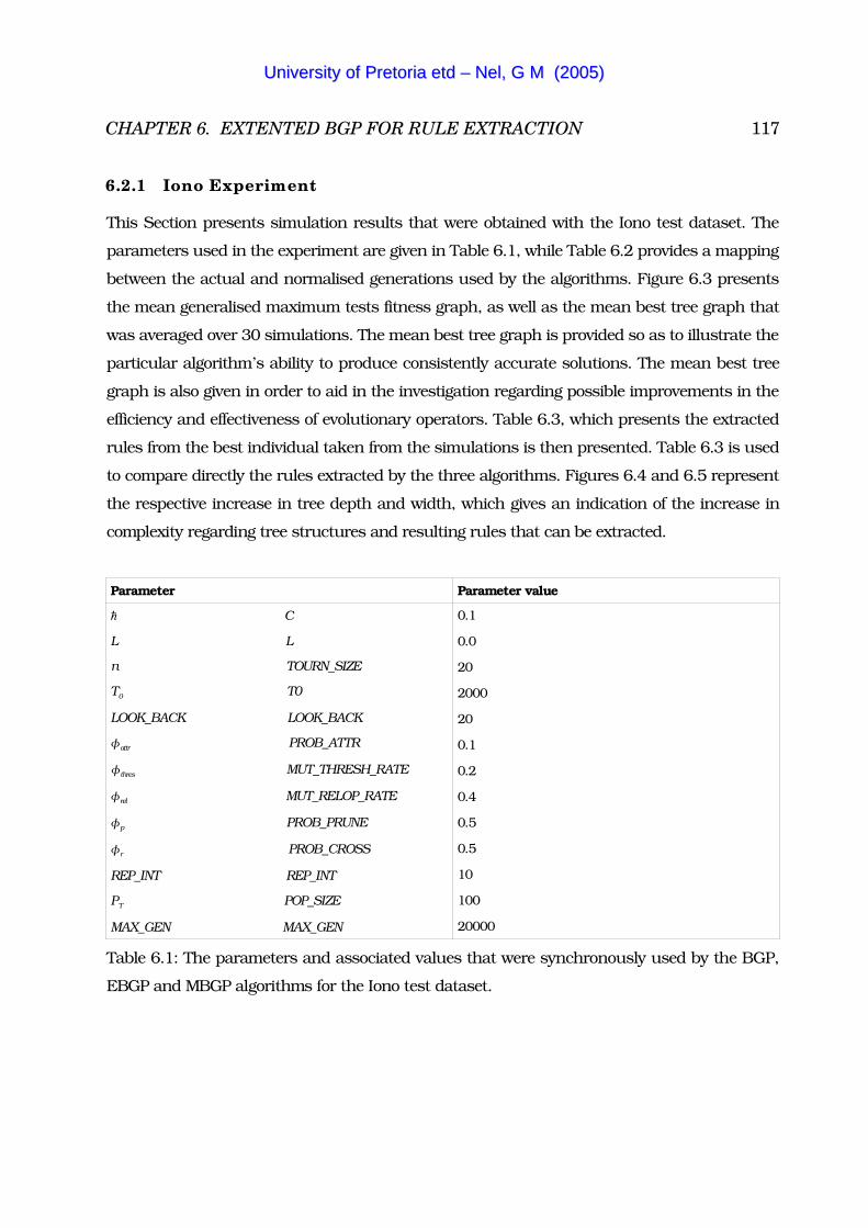
CHAPTER 6. EXTENTED BGP FOR RULE EXTRACTION 117
6.2.1 Iono Experiment
This Section presents simulation results that were obtained with the Iono test dataset. The
parameters used in the experiment are given in Table 6.1, while Table 6.2 provides a mapping
between the actual and normalised generations used by the algorithms. Figure 6.3 presents
the mean generalised maximum tests fitness graph, as well as the mean best tree graph that
was averaged over 30 simulations. The mean best tree graph is provided so as to illustrate the
particular algorithm’s ability to produce consistently accurate solutions. The mean best tree
graph is also given in order to aid in the investigation regarding possible improvements in the
efficiency and effectiveness of evolutionary operators. Table 6.3, which presents the extracted
rules from the best individual taken from the simulations is then presented. Table 6.3 is used
to compare directly the rules extracted by the three algorithms. Figures 6.4 and 6.5 represent
the respective increase in tree depth and width, which gives an indication of the increase in
complexity regarding tree structures and resulting rules that can be extracted.
Parameter Parameter value
� C
L L
n TOURN_SIZE
T0 T0
LOOK_BACK LOOK_BACK
�attr PROB_ATTR
�thres MUT_THRESH_RATE
�rel MUT_RELOP_RATE
�p PROB_PRUNE
�r PROB_CROSS
REP_INT REP_INT
PT POP_SIZE
MAX_GEN MAX_GEN
0.1
0.0
20
2000
20
0.1
0.2
0.4
0.5
0.5
10
100
20000
Table 6.1: The parameters and associated values that were synchronously used by the BGP,
EBGP and MBGP algorithms for the Iono test dataset.
UUnniivveerrssiittyy ooff PPrreettoorriiaa eettdd –– NNeell,, GG MM ((22000055))
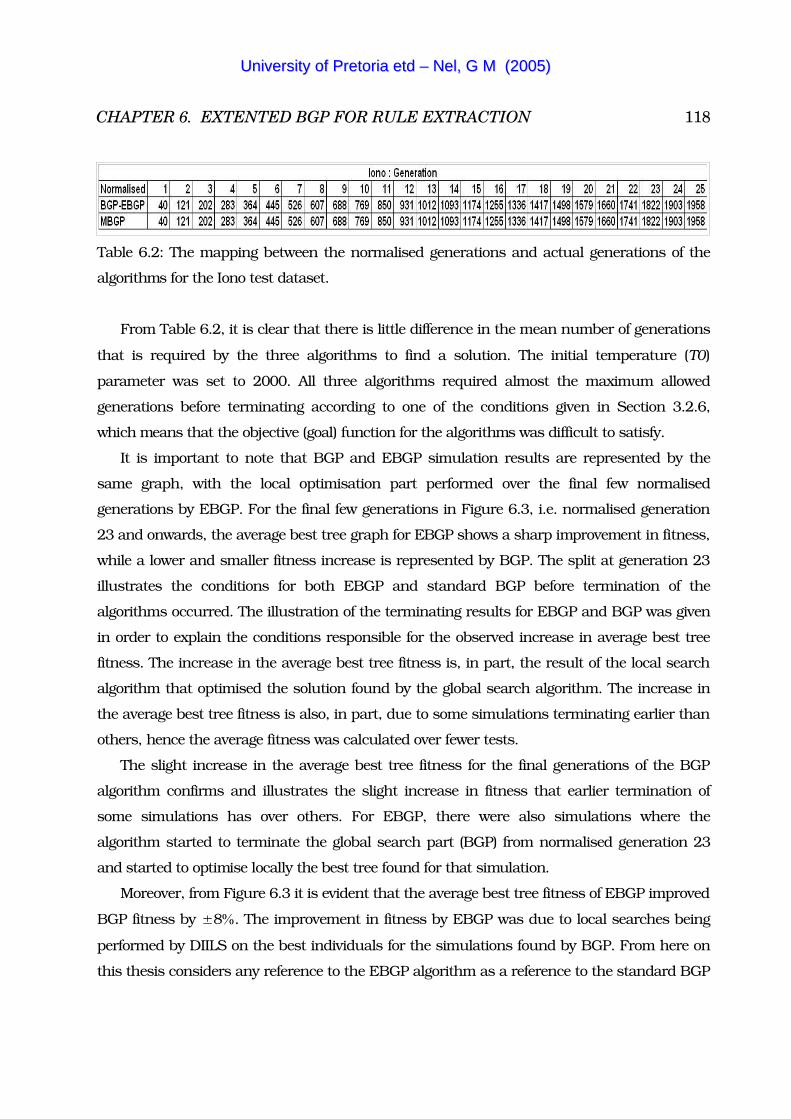
CHAPTER 6. EXTENTED BGP FOR RULE EXTRACTION 118
Table 6.2: The mapping between the normalised generations and actual generations of the
algorithms for the Iono test dataset.
From Table 6.2, it is clear that there is little difference in the mean number of generations
that is required by the three algorithms to find a solution. The initial temperature (T0)
parameter was set to 2000. All three algorithms required almost the maximum allowed
generations before terminating according to one of the conditions given in Section 3.2.6,
which means that the objective (goal) function for the algorithms was difficult to satisfy.
It is important to note that BGP and EBGP simulation results are represented by the
same graph, with the local optimisation part performed over the final few normalised
generations by EBGP. For the final few generations in Figure 6.3, i.e. normalised generation
23 and onwards, the average best tree graph for EBGP shows a sharp improvement in fitness,
while a lower and smaller fitness increase is represented by BGP. The split at generation 23
illustrates the conditions for both EBGP and standard BGP before termination of the
algorithms occurred. The illustration of the terminating results for EBGP and BGP was given
in order to explain the conditions responsible for the observed increase in average best tree
fitness. The increase in the average best tree fitness is, in part, the result of the local search
algorithm that optimised the solution found by the global search algorithm. The increase in
the average best tree fitness is also, in part, due to some simulations terminating earlier than
others, hence the average fitness was calculated over fewer tests.
The slight increase in the average best tree fitness for the final generations of the BGP
algorithm confirms and illustrates the slight increase in fitness that earlier termination of
some simulations has over others. For EBGP, there were also simulations where the
algorithm started to terminate the global search part (BGP) from normalised generation 23
and started to optimise locally the best tree found for that simulation.
Moreover, from Figure 6.3 it is evident that the average best tree fitness of EBGP improved
BGP fitness by �8. The improvement in fitness by EBGP was due to local searches being
performed by DIILS on the best individuals for the simulations found by BGP. From here on
this thesis considers any reference to the EBGP algorithm as a reference to the standard BGP
UUnniivveerrssiittyy ooff PPrreettoorriiaa eettdd –– NNeell,, GG MM ((22000055))
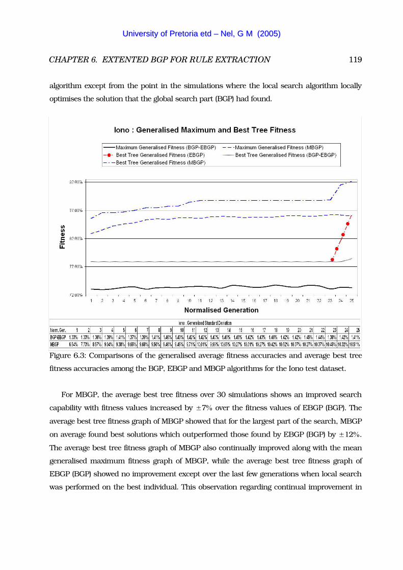
CHAPTER 6. EXTENTED BGP FOR RULE EXTRACTION 119
algorithm except from the point in the simulations where the local search algorithm locally
optimises the solution that the global search part (BGP) had found.
Figure 6.3: Comparisons of the generalised average fitness accuracies and average best tree
fitness accuracies among the BGP, EBGP and MBGP algorithms for the Iono test dataset.
For MBGP, the average best tree fitness over 30 simulations shows an improved search
capability with fitness values increased by �7 over the fitness values of EBGP (BGP). The
average best tree fitness graph of MBGP showed that for the largest part of the search, MBGP
on average found best solutions which outperformed those found by EBGP (BGP) by �12.
The average best tree fitness graph of MBGP also continually improved along with the mean
generalised maximum fitness graph of MBGP, while the average best tree fitness graph of
EBGP (BGP) showed no improvement except over the last few generations when local search
was performed on the best individual. This observation regarding continual improvement in
UUnniivveerrssiittyy ooff PPrreettoorriiaa eettdd –– NNeell,, GG MM ((22000055))
CHAPTER 6. EXTENTED BGP FOR RULE EXTRACTION 120
mean best tree fitness of MBGP provides support for the view that fitter building blocks
improve the efficiency and effectiveness of the evolutionary operators in exploring the search
space.
The mean generalised maximum test fitness of EBGP in Figure 6.3 confirms the notion
that the local search algorithm, and not the global search algorithm is responsible for the
improved best tree fitness since there was no appreciable variation in fitness over the
generations. Note that the mean generalised maximum fitness graph of EBGP represents only
the mean maximum fitness of the population of solutions found by the global search part
(BGP) of the algorithm. Local searches were performed only on those best individuals found
by the algorithm after the global searches terminated and were consequently not factored into
the mean generalised maximum test fitness graph. Hence, the evolutionary process did not
improve substantially the tree fitness, but local search applied afterwards did do so.
The graphs of the mean generalised maximum test fitness show that the initial fitness of
the MBGP population is significantly higher at �10 than the initial population fitness of
EBGP. Therefore, it is evident that the local search operator used to optimise the initial MBGP
population is responsible for the improved fitness. As a consequence a guarantee can be given
that the building blocks used by MBGP are locally optimised. The mean generalised
maximum fitness graph of MBGP also illustrates consistent improvement in fitness over the
generations. Notice that the mean generalised maximum fitness graph of MBGP initially had
an average fitness value of �83, and consistently improved over the generations by �3 to
a final average fitness of �86. On the other hand, the mean generalised maximum fitness
graph of EBGP showed little improvement of less than 1 from initial to final generations.
The consistent improvement exhibited by MBGP provides further evidence that fitter building
blocks used by MBGP, as compared to the building blocks used by EBGP, influence positively
the evolutionary operators to perform more efficiently with greater effectiveness, even though
the same parameter settings were used for all the algorithms.
Suppose that a termination condition for the algorithms was to terminate if no further
improvement could be made for a pre-determined number of generations. From the graphs in
Figure 6.3, MBGP would use more generations than EBGP to optimise a solution that is more
accurate. Hence, there is a trade off in this experiment between accuracy and speed for the
MBGP algorithm. However, notice the degree of accuracy achieved by MBGP over both EBGP
and BGP.
UUnniivveerrssiittyy ooff PPrreettoorriiaa eettdd –– NNeell,, GG MM ((22000055))

CHAPTER 6. EXTENTED BGP FOR RULE EXTRACTION 121
The standard deviation indicates the variability of the solutions found by the algorithms,
hence the stability of the solutions is also given in Figure 6.3. Section 4.4 reviewed the
method for calculating the normalised standard deviation values, which were performed in
the same fashion as the calculations done to determine the fitness values indicated by the
smoothed graphs in Figure 6.3. EBGP had little deviation in the fitness of the population of
solutions found by the algorithms over the generations. The notion of little fitness deviation in
the solutions found by EBGP is supported by both the relatively small variance in the mean
generalised maximum fitness graph, and the absence of improvement in the mean best tree
fitness graph of EBGP for a significantly greater number of the generations.
The standard deviation of �10 (see Figure 6.3) for MBGP provides evidence that the
solutions found by the algorithm had significantly more variance in terms of fitness. Two
conditions can create such large variances. The first is that the algorithm produces a
population of solutions from which more or less the same number of rules are extracted per
solution, but the rules extracted per solution has significant variances. The second condition
is that the number of rules extracted per solution increased, with the additional rules
introducing more variance. An increase in the tree complexity, in other words an increase in
tree width, will indicate whether additional rules were produced. An analysis of Figure 6.5 will
indicate which condition mentioned above had caused the standard deviation of MGBP to
increase so substantially and is discussed below.
UUnniivveerrssiittyy ooff PPrreettoorriiaa eettdd –– NNeell,, GG MM ((22000055))

CHAPTER 6. EXTENTED BGP FOR RULE EXTRACTION 122
BGP EBGP MBGP
Number of rules in tree: 3
The tree has depth: 3
The tree has width: 3
Accuracy on test set is: 94
Accuracy on training set is: 89
Rules:
IF A3 > A22
AND A5 < 0.315
THEN Class = Bad
(TrainAcc: 82, TestAcc: 100)
IF A3 > A22
AND A5 >= 0.315
THEN Class = Good
(TrainAcc: 91, TestAcc: 91)
IF A3 <= A22
THEN Class = Bad
(TrainAcc: 92, TestAcc: 100)
Number of rules in tree: 4
The tree has depth: 4
The tree has width: 4
Accuracy on test set is: 96
Accuracy on training set is: 89
Rules:
IF A5 > 0.018
AND A1 > 0.203
AND A18 >= -0.916
THEN Class = Good
(TrainAcc: 86, TestAcc: 94)
IF A5 > 0.018
AND A1 > 0.203
AND A18 < -0.916
THEN Class = Bad
(TrainAcc: 100, TestAcc: 100)
IF A5 > 0.018
AND A1 <= 0.203
THEN Class = Bad
(TrainAcc: 100, TestAcc: 100)
IF A5 <= 0.018
THEN Class = Bad
(TrainAcc: 100, TestAcc: 100)
Number of rules in tree: 8
The tree has depth: 8
The tree has width: 8
Accuracy on test set is: 98
Accuracy on training set is: 96
Rules:
IF A5 >= 0.039
AND A6 < -0.975
THEN Class = Bad
(TrainAcc: 100, TestAcc: 100)
IF A5 >= 0.039
AND A6 >= -0.975
AND A4 < -0.831
THEN Class = Bad
(TrainAcc: 91, TestAcc: 100)
IF A5 >= 0.039
AND A6 >= -0.975
AND A4 >= -0.831
AND A3 < 0.212
THEN Class = Bad
(TrainAcc: 92, TestAcc: 0)
IF A5 >= 0.039
AND A6 >= -0.975
AND A4 >= -0.831
AND A3 >= 0.212
AND A14 < -0.693
THEN Class = Bad
(TrainAcc: 67, TestAcc: 100)
(continued ...)
UUnniivveerrssiittyy ooff PPrreettoorriiaa eettdd –– NNeell,, GG MM ((22000055))

CHAPTER 6. EXTENTED BGP FOR RULE EXTRACTION 123
BGP EBGP MBGP
IF A5 >= 0.039
AND A6 >= -0.975
AND A4 >= -0.831
AND A3 >= 0.212
AND A14 >= -0.693
AND A8 > -0.226
THEN Class = Good
(TrainAcc: 95, TestAcc: 97)
IF A5 >= 0.039
AND A6 >= -0.975
AND A4 >= -0.831
AND A3 >= 0.212
AND A14 >= -0.693
AND A8 <= -0.226
AND A22 > 0.534
THEN Class = Bad
(TrainAcc: 100, TestAcc: 100)
IF A5 >= 0.039
AND A6 >= -0.975
AND A4 >= -0.831
AND A3 >= 0.212
AND A14 >= -0.693
AND A8 <= -0.226
AND A22 <= 0.534
THEN Class = Good
(TrainAcc: 93, TestAcc: 100)
IF A5 < 0.039
THEN Class = Bad
(TrainAcc: 100, TestAcc: 100)
Table 6.3: The respective rules of the best decision tree produced by BGP, EBGP and MBGP
algorithms for the Iono test dataset.
UUnniivveerrssiittyy ooff PPrreettoorriiaa eettdd –– NNeell,, GG MM ((22000055))
CHAPTER 6. EXTENTED BGP FOR RULE EXTRACTION 124
Table 6.3 indicates little difference in terms of complexity in the best tree found by both
the BGP and EBGP algorithms. Note that the best tree found for EBGP over the simulations is
different from the best tree found for BGP, since the best tree produced by BGP is not
necessarily the same tree after local optimisation was performed by EBGP. The fitness of the
best tree produced by the BGP algorithm over 30 simulations performed was 94. EBGP
found a best tree with a fitness of 96, giving an improved generalisation of 2 over standard
BGP. Notice that the training fitness of the best tree found was the same (89) for both
algorithms. Hence, the training fitness values are lower than the generalised fitness values for
the two algorithms, which indicate that the training process for both algorithms did not over-
fit the data. Considering the relative simplicity of the enhancement made by performing a
local optimisation on the solution produced by the global search algorithm and the
improvement finally obtained, the advantage of the EBGP algorithm is clear. MBGP found a
best tree with a fitness of 98 giving an improved generalisation of 4 over standard BGP
and 2 over EBGP.
An interesting observation is that the average best tree fitness value of the MBGP graph is
closer than the respective values for EBGP (BGP) to the fitness value for the best tree found by
MBGP in the simulations. This observation implies that MBGP produced best solutions over
the 30 simulations that were more consistently accurate than EBGP or BGP, even though
MBGP had a larger standard deviation while searching for the solutions. Analysis of the
remaining test datasets will confirm the notion that MBGP consistently produces solutions
over the simulations that are closer in accuracy to the best solution found in the simulations.
A further observation from Table 6.3, is that class ‘BAD’ was classified by some of the
rules of all three algorithms with a generalised accuracy of 100. However, the classification
of class ‘GOOD’ indicates that that BGP and EBGP each produced one rule with a respective
generalised classification accuracy of 91 and 94. MBGP produced two rules for class
‘GOOD’ with generalised accuracies of 97 and 100. Even though the Iono test case is a
classification problem with two classes as discussed in Section 4.1.1, it can be seen that the
ability to refine a solution that properly distinguishes between the classes available in the Iono
problem is better done by MBGP rather than by BGP or EBGP.
Table 6.3, along with Figures 6.4 and 6.5 provide further proof that MBGP produced more
complex tree structures in its population which were caused by the evolutionary operators
performing searches on fitter building blocks. Note that the more complex tree structures
UUnniivveerrssiittyy ooff PPrreettoorriiaa eettdd –– NNeell,, GG MM ((22000055))
CHAPTER 6. EXTENTED BGP FOR RULE EXTRACTION 125
were not generated at the cost of accuracy, but it was in fact improved. Consequently, more
complex rules were extracted with MBGP that better generalised the data. Recall that the
parameters were synchronised on all the algorithms during all simulations. A possible
explanation for the difference in tree structures in the population of the MBGP algorithm is
that evolutionary operators behave significantly different on building blocks that are highly fit.
The best tree found by MBGP has another interesting property. The average training
fitness of the best tree, which is 96, has only a 2 difference with the generalised fitness of
the tree, which is 98. There is a significantly larger difference in training fitness and
generalised fitness for the best trees produced by the BGP and EBGP algorithms. For EBGP
the difference is 7 while for BGP it is 5. Therefore, the rules produced by MBGP during the
training process classify the test data more consistently with a high accuracy. Note that there
is a rule present in the set of highly fit rules extracted from the best tree found by MBGP,
which is considered as ‘useless’ since it does not classify any test dataset instances. In other
words the ‘useless’ rule had a generalisation accuracy of 0. However, BGP and EBGP also
had small numbers of the ‘useless’ rules as part of their final rule sets in the best tree found
Tables in later experiments. This observation of some useless rules being part of the highly fit
rule set, along with the increase in tree structure complexity of MBGP strongly suggests that
either the probability to prune the individuals should be increased, or a more aggressive
pruning strategy should be employed.
Figure 6.4 illustrates how additional tree levels were added to the trees for the different
algorithms. The additional tree levels imply that more functions, given as the tuple in
equation (3.1), from the function set (explained in Section 3.1.3) were added to the trees.
Figure 6.5 illustrates the increase in the average branching factor that allowed more branches
to be created in the tree structures. As a consequence more rules were extracted per solution.
As can be expected, the complexity of trees produced by BGP and EBGP are exactly the same.
On the other hand, MBGP increased tree complexity by adding both more conditional clauses
(tree depth) and more rules (tree width).
UUnniivveerrssiittyy ooff PPrreettoorriiaa eettdd –– NNeell,, GG MM ((22000055))
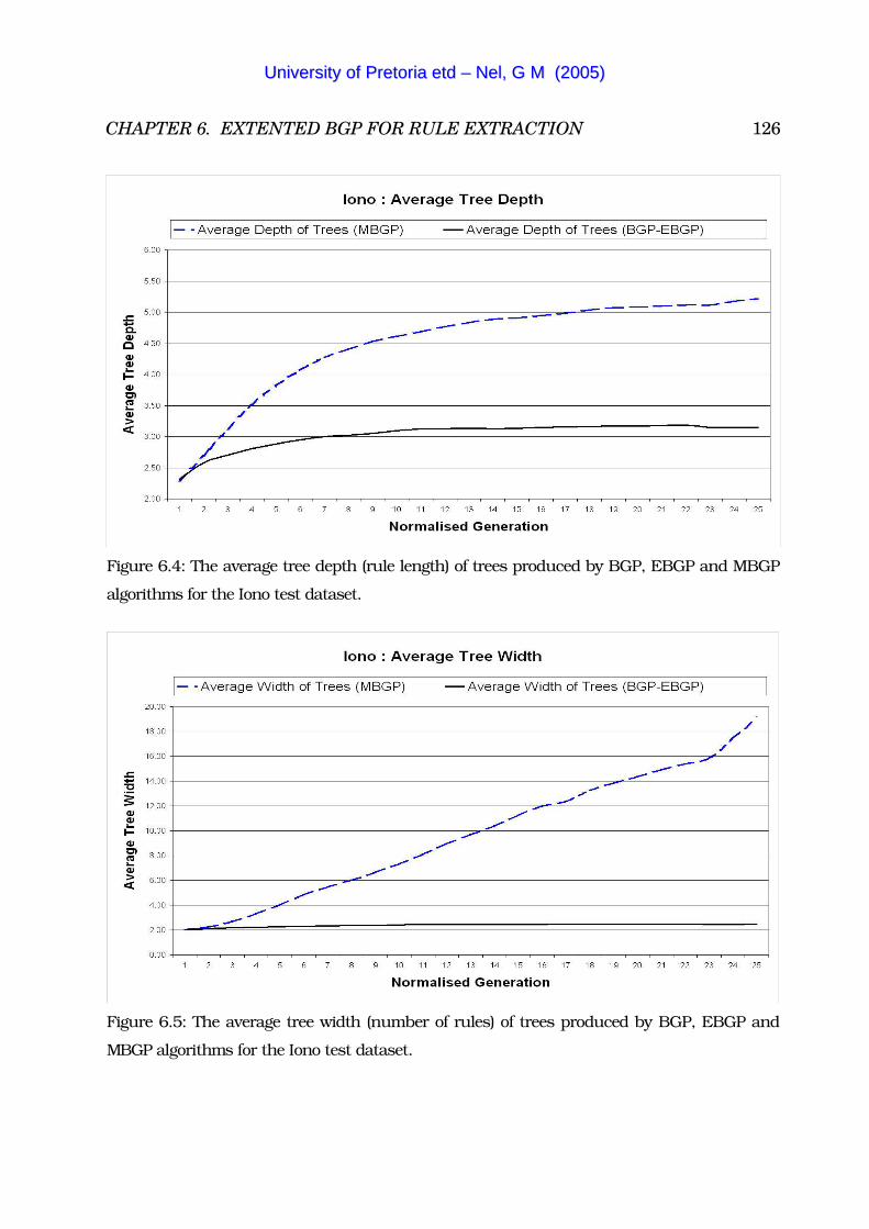
CHAPTER 6. EXTENTED BGP FOR RULE EXTRACTION 126
Figure 6.4: The average tree depth (rule length) of trees produced by BGP, EBGP and MBGP
algorithms for the Iono test dataset.
Figure 6.5: The average tree width (number of rules) of trees produced by BGP, EBGP and
MBGP algorithms for the Iono test dataset.
UUnniivveerrssiittyy ooff PPrreettoorriiaa eettdd –– NNeell,, GG MM ((22000055))
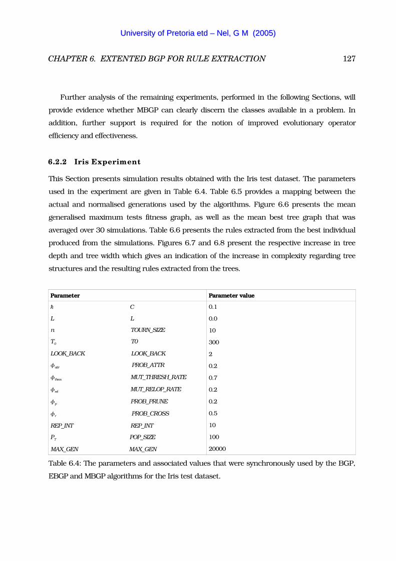
CHAPTER 6. EXTENTED BGP FOR RULE EXTRACTION 127
Further analysis of the remaining experiments, performed in the following Sections, will
provide evidence whether MBGP can clearly discern the classes available in a problem. In
addition, further support is required for the notion of improved evolutionary operator
efficiency and effectiveness.
6.2.2 Iris Experiment
This Section presents simulation results obtained with the Iris test dataset. The parameters
used in the experiment are given in Table 6.4. Table 6.5 provides a mapping between the
actual and normalised generations used by the algorithms. Figure 6.6 presents the mean
generalised maximum tests fitness graph, as well as the mean best tree graph that was
averaged over 30 simulations. Table 6.6 presents the rules extracted from the best individual
produced from the simulations. Figures 6.7 and 6.8 present the respective increase in tree
depth and tree width which gives an indication of the increase in complexity regarding tree
structures and the resulting rules extracted from the trees.
Parameter Parameter value
� C
L L
n TOURN_SIZE
T0 T0
LOOK_BACK LOOK_BACK
�attr PROB_ATTR
�thres MUT_THRESH_RATE
�rel MUT_RELOP_RATE
�p PROB_PRUNE
�r PROB_CROSS
REP_INT REP_INT
PT POP_SIZE
MAX_GEN MAX_GEN
0.1
0.0
10
300
2
0.2
0.7
0.2
0.2
0.5
10
100
20000
Table 6.4: The parameters and associated values that were synchronously used by the BGP,
EBGP and MBGP algorithms for the Iris test dataset.
UUnniivveerrssiittyy ooff PPrreettoorriiaa eettdd –– NNeell,, GG MM ((22000055))

CHAPTER 6. EXTENTED BGP FOR RULE EXTRACTION 128
Table 6.5: The mapping between the normalised generations and actual generations of the
algorithms for the Iris test dataset.
From Table 6.5 the observation is that the average number of generations used before the
algorithms terminated are almost the same for the EBGP and MBGP algorithms, with the
MBGP using more generations. Notice that T0 parameter was set to 300, which indicates that
the algorithms nearly required all the allowable generations.
Figure 6.6: Comparisons of the generalised average fitness accuracies and average best tree
fitness accuracies among the BGP, EBGP and MBGP algorithms for the Iris test dataset.
UUnniivveerrssiittyy ooff PPrreettoorriiaa eettdd –– NNeell,, GG MM ((22000055))
CHAPTER 6. EXTENTED BGP FOR RULE EXTRACTION 129
From Figure 6.6 the graph for EBGP illustrates how well the BGP and EBGP algorithms
learn in the first five normalised generations. After the fifth normalised generation, a relative
fitness plateau is reached for many generations thereafter where the fitness does not improve
much. Only in the last four normalised generations does the fitness of EBGP improve again.
Local search could not improve the solution found by BGP. Consequently, the average best
tree fitness found by EBGP is equal for this experiment to the average best tree fitness found
by BGP. It is evident from results obtained in this and the previous experiment that the
average fitness found by EBGP is greater than or equal to the average fitness found by BGP.
The mean generalised maximum fitness graph for EBGP shows an increase over the same
generations as the average best tree fitness graph. Hence, the global search part of EBGP,
which is the BGP algorithm, discovered a new region of the search space that contained more
accurate solutions. Recall that the last few generations are also the averaged fitness of fewer
simulations, since the algorithm started to terminate some of the simulations. Therefore,
fitness improvements are exaggerated in the last few generations. A further observation is that
the average best tree fitness graph of MBGP improved in fitness value only in the first three
normalised generations.
The mean generalised maximum fitness graph of MBGP continues the trend observed
with the Iono experiment. The graph starts with an initial population that is significantly more
fit, almost 25 more so than the starting populations of BGP or EBGP. An increase in fitness
of �7 is then achieved by MBGP within the first three normalised generations, where after
no further significant improvements are evident. Therefore, the MBGP algorithm can be
terminated after three normalised generations were used, and still produce a solution that is
significantly better than one produced by BGP or EBGP.
The standard deviations calculated for the algorithms with this experiment were
considerably higher than the previous experiment discussed in Section 6.2.1. This is an
indication that the population of solutions have significant variability in the accuracies of
rules produced. The standard deviation of MBGP is �17, which is, as it was found in
Section 6.2.1, higher than the standard deviation of EBGP. Note that the deviation for EBGP
is �10, which means that MBGP deviates by only �7 more than that of EBGP.
UUnniivveerrssiittyy ooff PPrreettoorriiaa eettdd –– NNeell,, GG MM ((22000055))
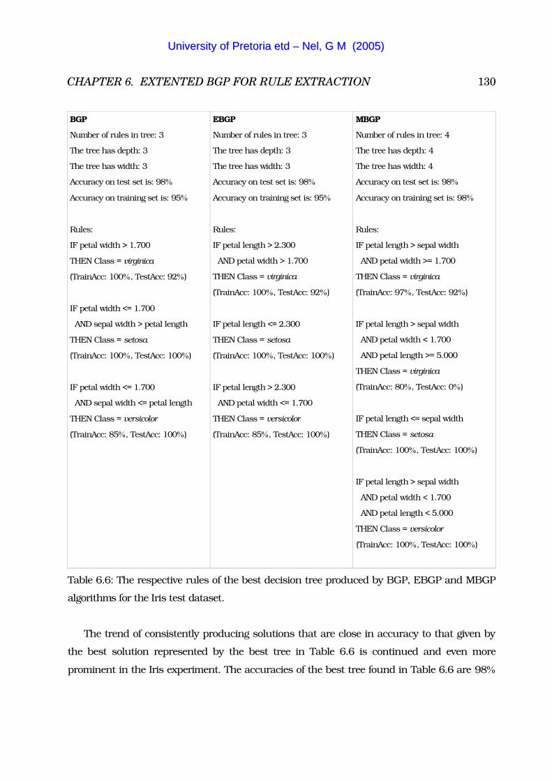
CHAPTER 6. EXTENTED BGP FOR RULE EXTRACTION 130
BGP EBGP MBGP
Number of rules in tree: 3
The tree has depth: 3
The tree has width: 3
Accuracy on test set is: 98
Accuracy on training set is: 95
Rules:
IF petal width > 1.700
THEN Class = virginica
(TrainAcc: 100, TestAcc: 92)
IF petal width <= 1.700
AND sepal width > petal length
THEN Class = setosa
(TrainAcc: 100, TestAcc: 100)
IF petal width <= 1.700
AND sepal width <= petal length
THEN Class = versicolor
(TrainAcc: 85, TestAcc: 100)
Number of rules in tree: 3
The tree has depth: 3
The tree has width: 3
Accuracy on test set is: 98
Accuracy on training set is: 95
Rules:
IF petal length > 2.300
AND petal width > 1.700
THEN Class = virginica
(TrainAcc: 100, TestAcc: 92)
IF petal length <= 2.300
THEN Class = setosa
(TrainAcc: 100, TestAcc: 100)
IF petal length > 2.300
AND petal width <= 1.700
THEN Class = versicolor
(TrainAcc: 85, TestAcc: 100)
Number of rules in tree: 4
The tree has depth: 4
The tree has width: 4
Accuracy on test set is: 98
Accuracy on training set is: 98
Rules:
IF petal length > sepal width
AND petal width >= 1.700
THEN Class = virginica
(TrainAcc: 97, TestAcc: 92)
IF petal length > sepal width
AND petal width < 1.700
AND petal length >= 5.000
THEN Class = virginica
(TrainAcc: 80, TestAcc: 0)
IF petal length <= sepal width
THEN Class = setosa
(TrainAcc: 100, TestAcc: 100)
IF petal length > sepal width
AND petal width < 1.700
AND petal length < 5.000
THEN Class = versicolor
(TrainAcc: 100, TestAcc: 100)
Table 6.6: The respective rules of the best decision tree produced by BGP, EBGP and MBGP
algorithms for the Iris test dataset.
The trend of consistently producing solutions that are close in accuracy to that given by
the best solution represented by the best tree in Table 6.6 is continued and even more
prominent in the Iris experiment. The accuracies of the best tree found in Table 6.6 are 98
UUnniivveerrssiittyy ooff PPrreettoorriiaa eettdd –– NNeell,, GG MM ((22000055))
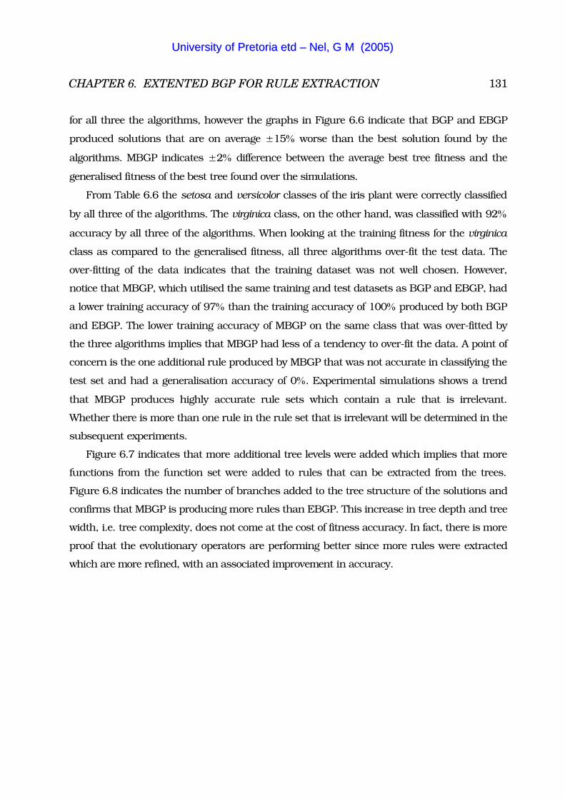
CHAPTER 6. EXTENTED BGP FOR RULE EXTRACTION 131
for all three the algorithms, however the graphs in Figure 6.6 indicate that BGP and EBGP
produced solutions that are on average �15 worse than the best solution found by the
algorithms. MBGP indicates �2 difference between the average best tree fitness and the
generalised fitness of the best tree found over the simulations.
From Table 6.6 the setosa and versicolor classes of the iris plant were correctly classified
by all three of the algorithms. The virginica class, on the other hand, was classified with 92
accuracy by all three of the algorithms. When looking at the training fitness for the virginica
class as compared to the generalised fitness, all three algorithms over-fit the test data. The
over-fitting of the data indicates that the training dataset was not well chosen. However,
notice that MBGP, which utilised the same training and test datasets as BGP and EBGP, had
a lower training accuracy of 97 than the training accuracy of 100 produced by both BGP
and EBGP. The lower training accuracy of MBGP on the same class that was over-fitted by
the three algorithms implies that MBGP had less of a tendency to over-fit the data. A point of
concern is the one additional rule produced by MBGP that was not accurate in classifying the
test set and had a generalisation accuracy of 0. Experimental simulations shows a trend
that MBGP produces highly accurate rule sets which contain a rule that is irrelevant.
Whether there is more than one rule in the rule set that is irrelevant will be determined in the
subsequent experiments.
Figure 6.7 indicates that more additional tree levels were added which implies that more
functions from the function set were added to rules that can be extracted from the trees.
Figure 6.8 indicates the number of branches added to the tree structure of the solutions and
confirms that MBGP is producing more rules than EBGP. This increase in tree depth and tree
width, i.e. tree complexity, does not come at the cost of fitness accuracy. In fact, there is more
proof that the evolutionary operators are performing better since more rules were extracted
which are more refined, with an associated improvement in accuracy.
UUnniivveerrssiittyy ooff PPrreettoorriiaa eettdd –– NNeell,, GG MM ((22000055))
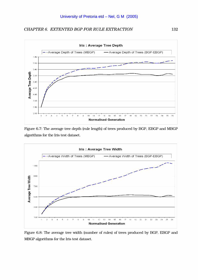
CHAPTER 6. EXTENTED BGP FOR RULE EXTRACTION 132
Figure 6.7: The average tree depth (rule length) of trees produced by BGP, EBGP and MBGP
algorithms for the Iris test dataset.
Figure 6.8: The average tree width (number of rules) of trees produced by BGP, EBGP and
MBGP algorithms for the Iris test dataset.
UUnniivveerrssiittyy ooff PPrreettoorriiaa eettdd –– NNeell,, GG MM ((22000055))

CHAPTER 6. EXTENTED BGP FOR RULE EXTRACTION 133
6.2.3 Monks1 Experiment
This Section presents simulation results obtained with the Monks1 test dataset. The
parameters used in the experiment are given in Table 6.7. Table 6.8 provides a mapping
between the actual and normalised generations used by the algorithms. Figure 6.9 presents
the mean generalised maximum tests fitness graph, as well as the mean best tree graph that
was averaged over 30 simulations. Table 6.9 shows the extracted rules from the best
individual taken from the simulations. Figures 6.10 and 6.11 present the respective increase
in tree depth and tree width which gives an indication of the increase in complexity regarding
tree structures and the resulting rules extracted.
Parameter Parameter value
� C
L L
n TOURN_SIZE
T0 T0
LOOK_BACK LOOK_BACK
�attr PROB_ATTR
�thres MUT_THRESH_RATE
�rel MUT_RELOP_RATE
�p PROB_PRUNE
�r PROB_CROSS
REP_INT REP_INT
PT POP_SIZE
MAX_GEN MAX_GEN
0.1
0.0
10
200
2
0.7
0.7
0.2
0.2
0.8
10
100
20000
Table 6.7: The parameters and associated values that were synchronously used by the BGP,
EBGP and MBGP algorithms for the Monks1 test dataset.
Table 6.8: The mapping between the normalised generations and actual generations of the
algorithms for the Monks1 test dataset.
UUnniivveerrssiittyy ooff PPrreettoorriiaa eettdd –– NNeell,, GG MM ((22000055))
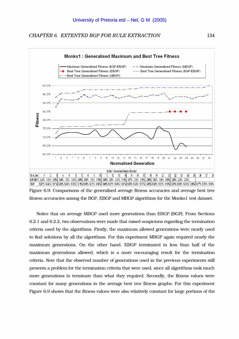
CHAPTER 6. EXTENTED BGP FOR RULE EXTRACTION 134
Figure 6.9: Comparisons of the generalised average fitness accuracies and average best tree
fitness accuracies among the BGP, EBGP and MBGP algorithms for the Monks1 test dataset.
Notice that on average MBGP used more generations than EBGP (BGP). From Sections
6.2.1 and 6.2.2, two observations were made that raised suspicions regarding the termination
criteria used by the algorithms. Firstly, the maximum allowed generations were nearly used
to find solutions by all the algorithms. For this experiment MBGP again required nearly the
maximum generations. On the other hand, EBGP terminated in less than half of the
maximum generations allowed, which is a more encouraging result for the termination
criteria. Note that the observed number of generations used in the previous experiments still
presents a problem for the termination criteria that were used, since all algorithms took much
more generations to terminate than what they required. Secondly, the fitness values were
constant for many generations in the average best tree fitness graphs. For this experiment
Figure 6.9 shows that the fitness values were also relatively constant for large portions of the
UUnniivveerrssiittyy ooff PPrreettoorriiaa eettdd –– NNeell,, GG MM ((22000055))
CHAPTER 6. EXTENTED BGP FOR RULE EXTRACTION 135
generations used in the average best tree graphs of MBGP and EBGP. Therefore, further
analysis is required of the experiments in Sections 6.2.4 to 6.2.6 to determine if the
termination criteria are in fact inefficient and/or ineffective in terminating the algorithms at
the correct temporal point.
From the average best tree fitness graph of EBGP (BGP) in Figure 6.9, it is evident that
BGP found solutions that cannot be improved by performing local optimisation as done by
EBGP. Notice that the average best tree fitness graphs for BGP and EBGP are not different at
any point. The average best tree fitness graph of EBGP also indicates that an increase of
�14 occurred from the initial fitness value to the termination fitness value. The best mean
fitness was reached by EBGP before normalised generation 15, which is just more than half of
the total generations that were used. Therefore, many more generations were used by EBGP
than the number required to find a solution of similar accuracy.
The MBGP algorithm continues the trend of starting with an initial population that has
higher fitness value than the starting populations of the BGP and EBGP algorithms. In
addition, the average best tree fitness value terminated with a significantly higher (�14)
fitness value, which means that the solutions found by MBGP had better accuracy over the
solutions that were found by either BGP or EBGP.
Of particular interest in Figure 6.9 is the mean generalised maximum fitness graph of
EBGP, because the graph shows large fluctuations in average fitness value over relatively few
generations. Note that the average best tree fitness graph of EBGP increased when the mean
generalised maximum fitness graph of EBGP increased. The increase in mean generalised
maximum fitness indicates that the population of individuals found a new region in the
search space that provided more accurate solutions, hence the associated increase in average
best tree fitness. Notice that the mean generalised maximum fitness graph of MBGP also has
the fluctuations in fitness value that were mentioned for EBGP. However, the fluctuations are
not as large as those present in the EBGP graph. Note also that the mean generalised
maximum fitness graph of MBGP never decreases to a point below the initial fitness value
found for the population.
UUnniivveerrssiittyy ooff PPrreettoorriiaa eettdd –– NNeell,, GG MM ((22000055))
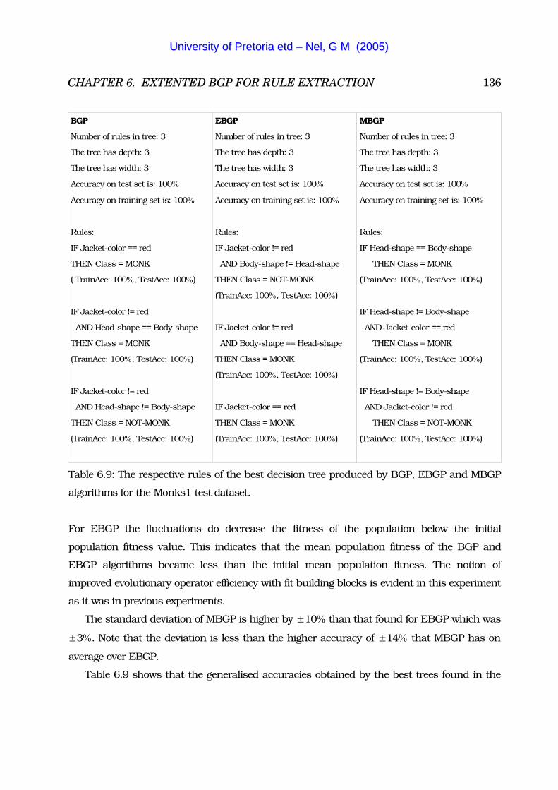
CHAPTER 6. EXTENTED BGP FOR RULE EXTRACTION 136
BGP EBGP MBGP
Number of rules in tree: 3
The tree has depth: 3
The tree has width: 3
Accuracy on test set is: 100
Accuracy on training set is: 100
Rules:
IF Jacket-color == red
THEN Class = MONK
( TrainAcc: 100, TestAcc: 100)
IF Jacket-color != red
AND Head-shape == Body-shape
THEN Class = MONK
(TrainAcc: 100, TestAcc: 100)
IF Jacket-color != red
AND Head-shape != Body-shape
THEN Class = NOT-MONK
(TrainAcc: 100, TestAcc: 100)
Number of rules in tree: 3
The tree has depth: 3
The tree has width: 3
Accuracy on test set is: 100
Accuracy on training set is: 100
Rules:
IF Jacket-color != red
AND Body-shape != Head-shape
THEN Class = NOT-MONK
(TrainAcc: 100, TestAcc: 100)
IF Jacket-color != red
AND Body-shape == Head-shape
THEN Class = MONK
(TrainAcc: 100, TestAcc: 100)
IF Jacket-color == red
THEN Class = MONK
(TrainAcc: 100, TestAcc: 100)
Number of rules in tree: 3
The tree has depth: 3
The tree has width: 3
Accuracy on test set is: 100
Accuracy on training set is: 100
Rules:
IF Head-shape == Body-shape
THEN Class = MONK
(TrainAcc: 100, TestAcc: 100)
IF Head-shape != Body-shape
AND Jacket-color == red
THEN Class = MONK
(TrainAcc: 100, TestAcc: 100)
IF Head-shape != Body-shape
AND Jacket-color != red
THEN Class = NOT-MONK
(TrainAcc: 100, TestAcc: 100)
Table 6.9: The respective rules of the best decision tree produced by BGP, EBGP and MBGP
algorithms for the Monks1 test dataset.
For EBGP the fluctuations do decrease the fitness of the population below the initial
population fitness value. This indicates that the mean population fitness of the BGP and
EBGP algorithms became less than the initial mean population fitness. The notion of
improved evolutionary operator efficiency with fit building blocks is evident in this experiment
as it was in previous experiments.
The standard deviation of MBGP is higher by �10 than that found for EBGP which was
�3. Note that the deviation is less than the higher accuracy of �14 that MBGP has on
average over EBGP.
Table 6.9 shows that the generalised accuracies obtained by the best trees found in the
UUnniivveerrssiittyy ooff PPrreettoorriiaa eettdd –– NNeell,, GG MM ((22000055))
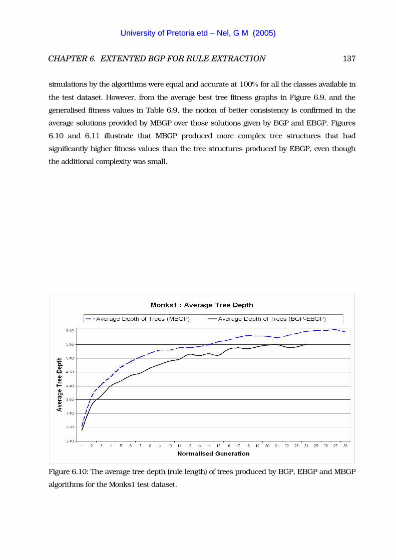
CHAPTER 6. EXTENTED BGP FOR RULE EXTRACTION 137
simulations by the algorithms were equal and accurate at 100 for all the classes available in
the test dataset. However, from the average best tree fitness graphs in Figure 6.9, and the
generalised fitness values in Table 6.9, the notion of better consistency is confirmed in the
average solutions provided by MBGP over those solutions given by BGP and EBGP. Figures
6.10 and 6.11 illustrate that MBGP produced more complex tree structures that had
significantly higher fitness values than the tree structures produced by EBGP, even though
the additional complexity was small.
Figure 6.10: The average tree depth (rule length) of trees produced by BGP, EBGP and MBGP
algorithms for the Monks1 test dataset.
UUnniivveerrssiittyy ooff PPrreettoorriiaa eettdd –– NNeell,, GG MM ((22000055))
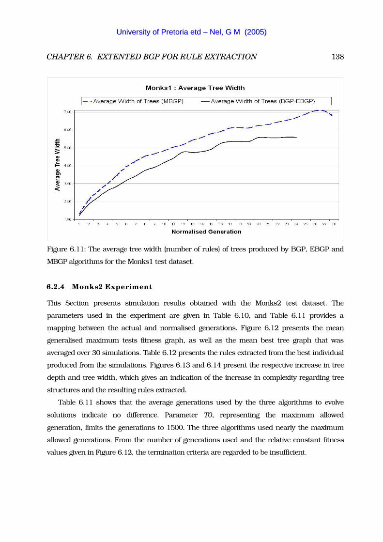
CHAPTER 6. EXTENTED BGP FOR RULE EXTRACTION 138
Figure 6.11: The average tree width (number of rules) of trees produced by BGP, EBGP and
MBGP algorithms for the Monks1 test dataset.
6.2.4 Monks2 Experiment
This Section presents simulation results obtained with the Monks2 test dataset. The
parameters used in the experiment are given in Table 6.10, and Table 6.11 provides a
mapping between the actual and normalised generations. Figure 6.12 presents the mean
generalised maximum tests fitness graph, as well as the mean best tree graph that was
averaged over 30 simulations. Table 6.12 presents the rules extracted from the best individual
produced from the simulations. Figures 6.13 and 6.14 present the respective increase in tree
depth and tree width, which gives an indication of the increase in complexity regarding tree
structures and the resulting rules extracted.
Table 6.11 shows that the average generations used by the three algorithms to evolve
solutions indicate no difference. Parameter T0, representing the maximum allowed
generation, limits the generations to 1500. The three algorithms used nearly the maximum
allowed generations. From the number of generations used and the relative constant fitness
values given in Figure 6.12, the termination criteria are regarded to be insufficient.
UUnniivveerrssiittyy ooff PPrreettoorriiaa eettdd –– NNeell,, GG MM ((22000055))
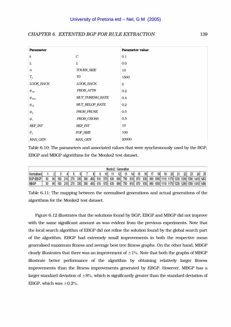
CHAPTER 6. EXTENTED BGP FOR RULE EXTRACTION 139
Parameter Parameter value
� C
L L
n TOURN_SIZE
T0 T0
LOOK_BACK LOOK_BACK
�attr PROB_ATTR
�thres MUT_THRESH_RATE
�rel MUT_RELOP_RATE
�p PROB_PRUNE
�r PROB_CROSS
REP_INT REP_INT
PT POP_SIZE
MAX_GEN MAX_GEN
0.1
0.0
10
1500
2
0.2
0.4
0.2
0.5
0.5
10
100
20000
Table 6.10: The parameters and associated values that were synchronously used by the BGP,
EBGP and MBGP algorithms for the Monks2 test dataset.
Table 6.11: The mapping between the normalised generations and actual generations of the
algorithms for the Monks2 test dataset.
Figure 6.12 illustrates that the solutions found by BGP, EBGP and MBGP did not improve
with the same significant amount as was evident from the previous experiments. Note that
the local search algorithm of EBGP did not refine the solution found by the global search part
of the algorithm. EBGP had extremely small improvements in both the respective mean
generalised maximum fitness and average best tree fitness graphs. On the other hand, MBGP
clearly illustrates that there was an improvement of �1. Note that both the graphs of MBGP
illustrate better performance of the algorithm by obtaining relatively larger fitness
improvements than the fitness improvements generated by EBGP. However, MBGP has a
larger standard deviation of �8, which is significantly greater than the standard deviation of
EBGP, which was �0.2.
UUnniivveerrssiittyy ooff PPrreettoorriiaa eettdd –– NNeell,, GG MM ((22000055))
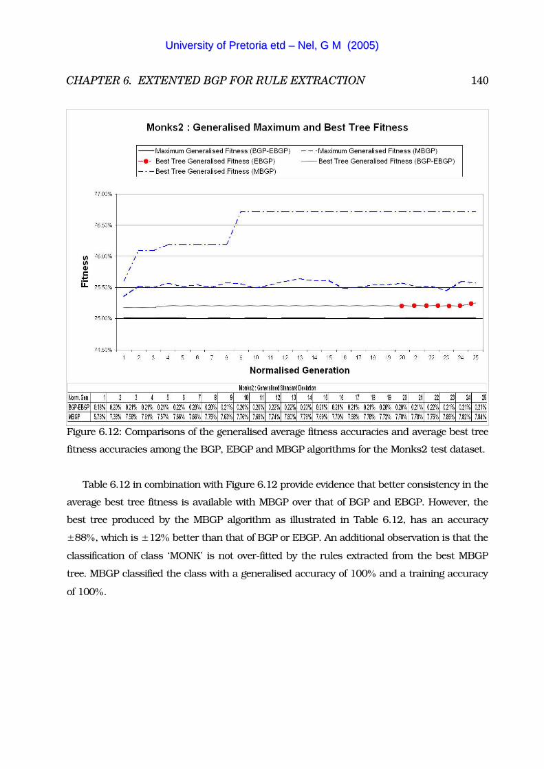
CHAPTER 6. EXTENTED BGP FOR RULE EXTRACTION 140
Figure 6.12: Comparisons of the generalised average fitness accuracies and average best tree
fitness accuracies among the BGP, EBGP and MBGP algorithms for the Monks2 test dataset.
Table 6.12 in combination with Figure 6.12 provide evidence that better consistency in the
average best tree fitness is available with MBGP over that of BGP and EBGP. However, the
best tree produced by the MBGP algorithm as illustrated in Table 6.12, has an accuracy
�88, which is �12 better than that of BGP or EBGP. An additional observation is that the
classification of class ‘MONK’ is not over-fitted by the rules extracted from the best MBGP
tree. MBGP classified the class with a generalised accuracy of 100 and a training accuracy
of 100.
UUnniivveerrssiittyy ooff PPrreettoorriiaa eettdd –– NNeell,, GG MM ((22000055))

CHAPTER 6. EXTENTED BGP FOR RULE EXTRACTION 141
BGP EBGP MBGP
Number of rules in tree: 6
The tree has depth: 6
The tree has width: 6
Accuracy on test set is: 76
Accuracy on training set is: 71
Rules:
IF A4 != A5
AND A1 == A4
THEN Class = NOT-MONK
(TrainAcc: 69, TestAcc: 74)
IF A4 != A5
AND A1 != A4
AND A4 == 2
THEN Class = NOT-MONK
(TrainAcc: 57, TestAcc: 79)
IF A4 != A5
AND A1 != A4
AND A4 != 2
AND A3 == A6
THEN Class = NOT-MONK
(TrainAcc: 76, TestAcc: 87)
IF A4 != A5
AND A1 != A4
AND A4 != 2
AND A3 != A6
AND A2 == 1
THEN Class = NOT-MONK
(TrainAcc: 75, TestAcc: 100)
Number of rules in tree: 6
The tree has depth: 6
The tree has width: 6
Accuracy on test set is: 77
Accuracy on training set is: 71
Rules:
IF A4 != A3
AND A6 == A1
THEN Class = NOT-MONK
(TrainAcc: 73, TestAcc: 88)
IF A4 != A3
AND A6 != A1
AND A6 != A5
AND A3 == 1
AND A2 == 1
THEN Class = NOT-MONK
(TrainAcc: 93, TestAcc: 67)
IF A4 != A3
AND A6 != A1
AND A6 != A5
AND A3 == 1
AND A2 != 1
THEN Class = MONK
(TrainAcc: 89, TestAcc: 57)
IF A4 != A3
AND A6 != A1
AND A6 == A5
THEN Class = NOT-MONK
(TrainAcc: 69, TestAcc: 75)
Number of rules in tree: 13
The tree has depth: 6
The tree has width: 13
Accuracy on test set is: 88
Accuracy on training set is: 84
Rules:
IF A3 == A6
AND A3 == 1
THEN Class = NOT-MONK
(TrainAcc: 78, TestAcc: 78)
IF A3 != A6
AND A4 != 1
AND A1 == 1
AND A1 != A2
AND A5 == A1
THEN Class = NOT-MONK
(TrainAcc: 100, TestAcc: 100)
IF A3 != A6
AND A4 == 1
AND A1 == 1
THEN Class = NOT-MONK
(TrainAcc: 100, TestAcc: 100)
IF A3 != A6
AND A4 != 1
AND A1 != 1
AND A2 == 1
THEN Class = MONK
(TrainAcc: 75, TestAcc: 75)
(continued ...)
UUnniivveerrssiittyy ooff PPrreettoorriiaa eettdd –– NNeell,, GG MM ((22000055))

CHAPTER 6. EXTENTED BGP FOR RULE EXTRACTION 142
BGP EBGP MBGP
IF A4 != A5
AND A1 != A4
AND A4 != 2
AND A3 != A6
AND A2 != 1
THEN Class = MONK
(TrainAcc: 79, TestAcc: 56)
IF A4 == A5
THEN Class = NOT-MONK
(TrainAcc: 74, TestAcc: 67)
IF A4 != A3
AND A6 != A1
AND A6 != A5
AND A3 != 1
THEN Class = NOT-MONK
(TrainAcc: 52, TestAcc: 72)
IF A4 == A3
THEN Class = NOT-MONK
(TrainAcc: 71, TestAcc: 85)
IF A3 != A6
AND A4 != 1
AND A1 == 1
AND A1 != A2
AND A5 != A1
THEN Class = MONK
(TrainAcc: 100, TestAcc: 100)
IF A3 != A6
AND A4 != 1
AND A1 == 1
AND A1 == A2
AND A1 != A6
THEN Class = NOT-MONK
(TrainAcc: 100, TestAcc: 100)
IF A3 != A6
AND A4 != 1
AND A1 == 1
AND A1 == A2
AND A1 == A6
THEN Class = NOT-MONK
(TrainAcc: 100, TestAcc: 100)
IF A3 != A6
AND A4 == 1
AND A1 != 1
AND A2 != A4
AND A5 != A4
THEN Class = MONK
(TrainAcc: 100, TestAcc: 100)
(continued ...)
UUnniivveerrssiittyy ooff PPrreettoorriiaa eettdd –– NNeell,, GG MM ((22000055))

CHAPTER 6. EXTENTED BGP FOR RULE EXTRACTION 143
BGP EBGP MBGP
IF A3 != A6
AND A4 != 1
AND A1 != 1
AND A2 != 1
AND A5 != 1
THEN Class = NOT-MONK
(TrainAcc: 100, TestAcc: 100)
IF A3 != A6
AND A4 != 1
AND A1 != 1
AND A2 != 1
AND A5 == 1
THEN Class = MONK
(TrainAcc: 100, TestAcc: 100)
IF A3 != A6
AND A4 == 1
AND A1 != 1
AND A2 != A4
AND A5 == A4
THEN Class = NOT-MONK
(TrainAcc: 100, TestAcc: 100)
IF A3 != A6
AND A4 == 1
AND A1 != 1
AND A2 == A4
THEN Class = NOT-MONK
(TrainAcc: 100, TestAcc: 100)
(continued ...)
UUnniivveerrssiittyy ooff PPrreettoorriiaa eettdd –– NNeell,, GG MM ((22000055))
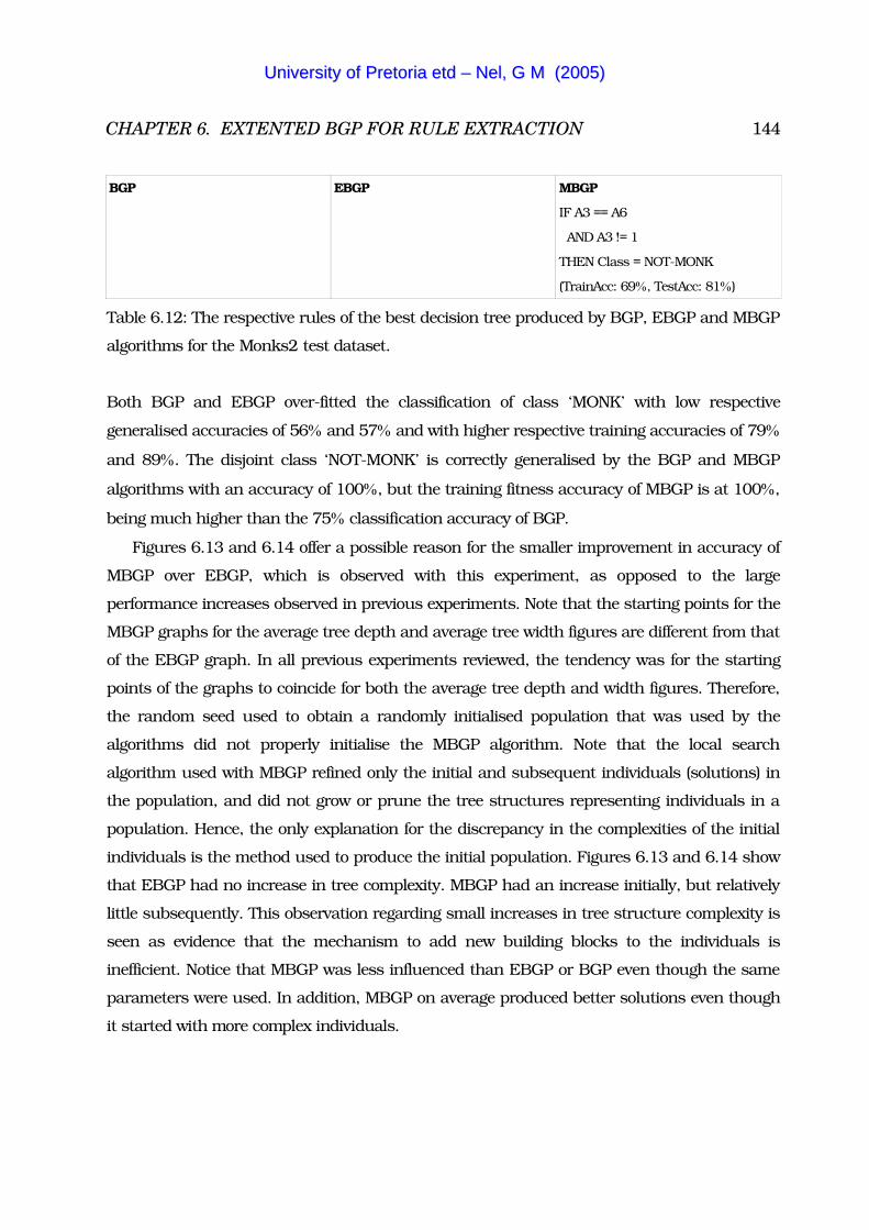
CHAPTER 6. EXTENTED BGP FOR RULE EXTRACTION 144
BGP EBGP MBGP
IF A3 == A6
AND A3 != 1
THEN Class = NOT-MONK
(TrainAcc: 69, TestAcc: 81)
Table 6.12: The respective rules of the best decision tree produced by BGP, EBGP and MBGP
algorithms for the Monks2 test dataset.
Both BGP and EBGP over-fitted the classification of class ‘MONK’ with low respective
generalised accuracies of 56 and 57 and with higher respective training accuracies of 79
and 89. The disjoint class ‘NOT-MONK’ is correctly generalised by the BGP and MBGP
algorithms with an accuracy of 100, but the training fitness accuracy of MBGP is at 100,
being much higher than the 75 classification accuracy of BGP.
Figures 6.13 and 6.14 offer a possible reason for the smaller improvement in accuracy of
MBGP over EBGP, which is observed with this experiment, as opposed to the large
performance increases observed in previous experiments. Note that the starting points for the
MBGP graphs for the average tree depth and average tree width figures are different from that
of the EBGP graph. In all previous experiments reviewed, the tendency was for the starting
points of the graphs to coincide for both the average tree depth and width figures. Therefore,
the random seed used to obtain a randomly initialised population that was used by the
algorithms did not properly initialise the MBGP algorithm. Note that the local search
algorithm used with MBGP refined only the initial and subsequent individuals (solutions) in
the population, and did not grow or prune the tree structures representing individuals in a
population. Hence, the only explanation for the discrepancy in the complexities of the initial
individuals is the method used to produce the initial population. Figures 6.13 and 6.14 show
that EBGP had no increase in tree complexity. MBGP had an increase initially, but relatively
little subsequently. This observation regarding small increases in tree structure complexity is
seen as evidence that the mechanism to add new building blocks to the individuals is
inefficient. Notice that MBGP was less influenced than EBGP or BGP even though the same
parameters were used. In addition, MBGP on average produced better solutions even though
it started with more complex individuals.
UUnniivveerrssiittyy ooff PPrreettoorriiaa eettdd –– NNeell,, GG MM ((22000055))
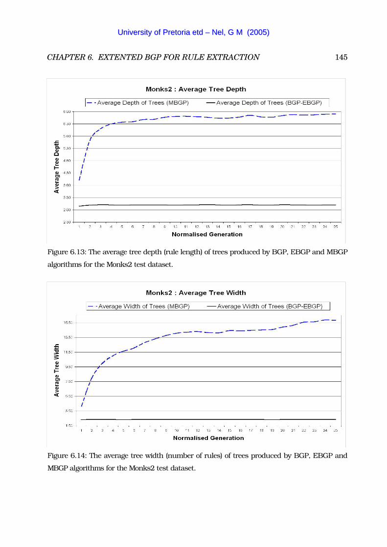
CHAPTER 6. EXTENTED BGP FOR RULE EXTRACTION 145
Figure 6.13: The average tree depth (rule length) of trees produced by BGP, EBGP and MBGP
algorithms for the Monks2 test dataset.
Figure 6.14: The average tree width (number of rules) of trees produced by BGP, EBGP and
MBGP algorithms for the Monks2 test dataset.
UUnniivveerrssiittyy ooff PPrreettoorriiaa eettdd –– NNeell,, GG MM ((22000055))
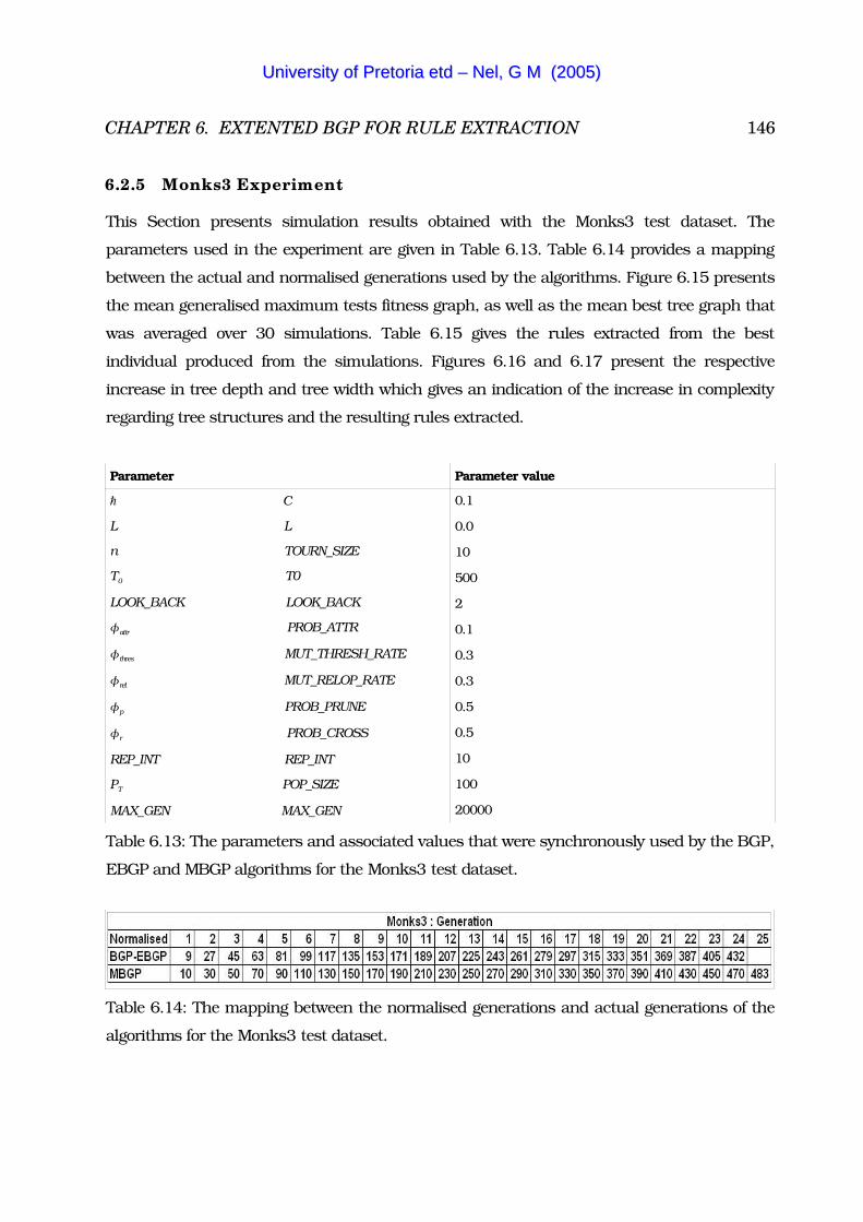
CHAPTER 6. EXTENTED BGP FOR RULE EXTRACTION 146
6.2.5 Monks3 Experiment
This Section presents simulation results obtained with the Monks3 test dataset. The
parameters used in the experiment are given in Table 6.13. Table 6.14 provides a mapping
between the actual and normalised generations used by the algorithms. Figure 6.15 presents
the mean generalised maximum tests fitness graph, as well as the mean best tree graph that
was averaged over 30 simulations. Table 6.15 gives the rules extracted from the best
individual produced from the simulations. Figures 6.16 and 6.17 present the respective
increase in tree depth and tree width which gives an indication of the increase in complexity
regarding tree structures and the resulting rules extracted.
Parameter Parameter value
� C
L L
n TOURN_SIZE
T0 T0
LOOK_BACK LOOK_BACK
�attr PROB_ATTR
�thres MUT_THRESH_RATE
�rel MUT_RELOP_RATE
�p PROB_PRUNE
�r PROB_CROSS
REP_INT REP_INT
PT POP_SIZE
MAX_GEN MAX_GEN
0.1
0.0
10
500
2
0.1
0.3
0.3
0.5
0.5
10
100
20000
Table 6.13: The parameters and associated values that were synchronously used by the BGP,
EBGP and MBGP algorithms for the Monks3 test dataset.
Table 6.14: The mapping between the normalised generations and actual generations of the
algorithms for the Monks3 test dataset.
UUnniivveerrssiittyy ooff PPrreettoorriiaa eettdd –– NNeell,, GG MM ((22000055))
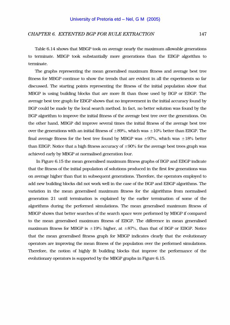
CHAPTER 6. EXTENTED BGP FOR RULE EXTRACTION 147
Table 6.14 shows that MBGP took on average nearly the maximum allowable generations
to terminate. MBGP took substantially more generations than the EBGP algorithm to
terminate.
The graphs representing the mean generalised maximum fitness and average best tree
fitness for MBGP continue to show the trends that are evident in all the experiments so far
discussed. The starting points representing the fitness of the initial population show that
MBGP is using building blocks that are more fit than those used by BGP or EBGP. The
average best tree graph for EBGP shows that no improvement in the initial accuracy found by
BGP could be made by the local search method. In fact, no better solution was found by the
BGP algorithm to improve the initial fitness of the average best tree over the generations. On
the other hand, MBGP did improve several times the initial fitness of the average best tree
over the generations with an initial fitness of �89, which was �10 better than EBGP. The
final average fitness for the best tree found by MBGP was �97, which was �18 better
than EBGP. Notice that a high fitness accuracy of �90 for the average best trees graph was
achieved early by MBGP at normalised generation four.
In Figure 6.15 the mean generalised maximum fitness graphs of BGP and EBGP indicate
that the fitness of the initial population of solutions produced in the first few generations was
on average higher than that in subsequent generations. Therefore, the operators employed to
add new building blocks did not work well in the case of the BGP and EBGP algorithms. The
variation in the mean generalised maximum fitness for the algorithms from normalised
generation 21 until termination is explained by the earlier termination of some of the
algorithms during the performed simulations. The mean generalised maximum fitness of
MBGP shows that better searches of the search space were performed by MBGP if compared
to the mean generalised maximum fitness of EBGP. The difference in mean generalised
maximum fitness for MBGP is �19 higher, at �87, than that of BGP or EBGP. Notice
that the mean generalised fitness graph for MBGP indicates clearly that the evolutionary
operators are improving the mean fitness of the population over the performed simulations.
Therefore, the notion of highly fit building blocks that improve the performance of the
evolutionary operators is supported by the MBGP graphs in Figure 6.15.
UUnniivveerrssiittyy ooff PPrreettoorriiaa eettdd –– NNeell,, GG MM ((22000055))
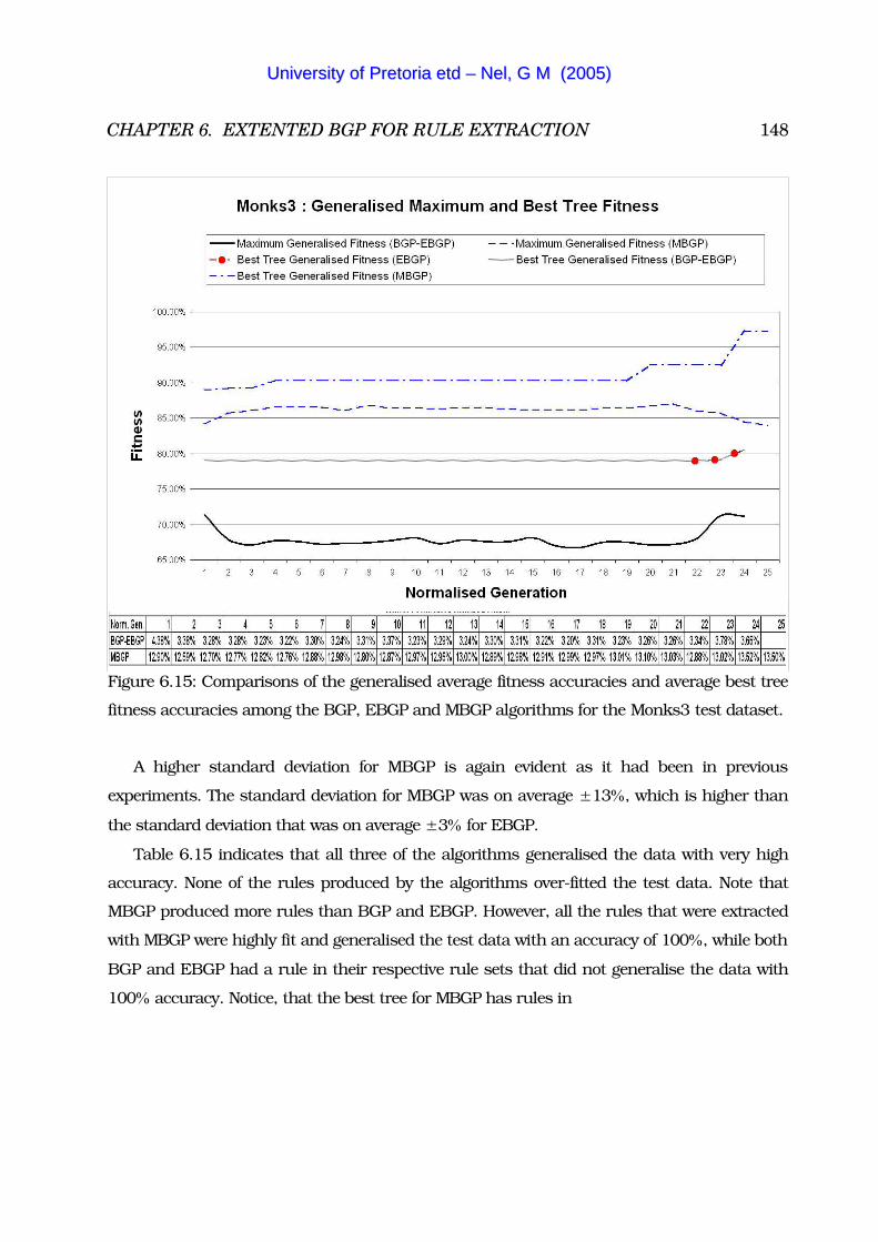
CHAPTER 6. EXTENTED BGP FOR RULE EXTRACTION 148
Figure 6.15: Comparisons of the generalised average fitness accuracies and average best tree
fitness accuracies among the BGP, EBGP and MBGP algorithms for the Monks3 test dataset.
A higher standard deviation for MBGP is again evident as it had been in previous
experiments. The standard deviation for MBGP was on average �13, which is higher than
the standard deviation that was on average �3 for EBGP.
Table 6.15 indicates that all three of the algorithms generalised the data with very high
accuracy. None of the rules produced by the algorithms over-fitted the test data. Note that
MBGP produced more rules than BGP and EBGP. However, all the rules that were extracted
with MBGP were highly fit and generalised the test data with an accuracy of 100, while both
BGP and EBGP had a rule in their respective rule sets that did not generalise the data with
100 accuracy. Notice, that the best tree for MBGP has rules in
UUnniivveerrssiittyy ooff PPrreettoorriiaa eettdd –– NNeell,, GG MM ((22000055))

CHAPTER 6. EXTENTED BGP FOR RULE EXTRACTION 149
BGP EBGP MBGP
Number of rules in tree: 3
The tree has depth: 3
The tree has width: 3
Accuracy on test set is: 97
Accuracy on training set is: 93
Rules:
IF A2 != 3
AND A5 == 4
THEN Class = NOT-MONK
(TrainAcc: 100, TestAcc: 100)
IF A2 != 3
AND A5 != 4
THEN Class = MONK
(TrainAcc: 92, TestAcc: 100)
IF A2 == 3
THEN Class = NOT-MONK
(TrainAcc: 93, TestAcc: 92)
Number of rules in tree: 5
The tree has depth: 4
The tree has width: 5
Accuracy on test set is: 97
Accuracy on training set is: 93
Rules:
IF A5 == 4
AND A3 != 1
THEN Class = NOT-MONK
(TrainAcc: 100, TestAcc: 100)
IF A5 == 4
AND A3 == 1
AND A6 != 2
THEN Class = NOT-MONK
(TrainAcc: 89, TestAcc: 100)
IF A5 == 4
AND A3 == 1
AND A6 == 2
THEN Class = NOT-MONK
(TrainAcc: 100, TestAcc: 100)
IF A5 != 4
AND A2 == 3
THEN Class = NOT-MONK
(TrainAcc: 93, TestAcc: 89)
IF A5 != 4
AND A2 != 3
THEN Class = MONK
(TrainAcc: 92, TestAcc: 100)
Number of rules in tree: 6
The tree has depth: 4
The tree has width: 6
Accuracy on test set is: 100
Accuracy on training set is: 95
Rules:
IF A5 == 3
AND A2 != 3
THEN Class = MONK
(TrainAcc: 78, TestAcc: 100)
IF A5 == 3
AND A2 == 3
AND A4 != 1
THEN Class = NOT-MONK
(TrainAcc: 100, TestAcc: 100)
IF A5 == 3
AND A2 == 3
AND A4 == 1
THEN Class = MONK
(TrainAcc: 100, TestAcc: 100)
IF A5 != 3
AND A2 != 3
AND A5 != 4
THEN Class = MONK
(TrainAcc: 98, TestAcc: 100)
(continued ...)
UUnniivveerrssiittyy ooff PPrreettoorriiaa eettdd –– NNeell,, GG MM ((22000055))
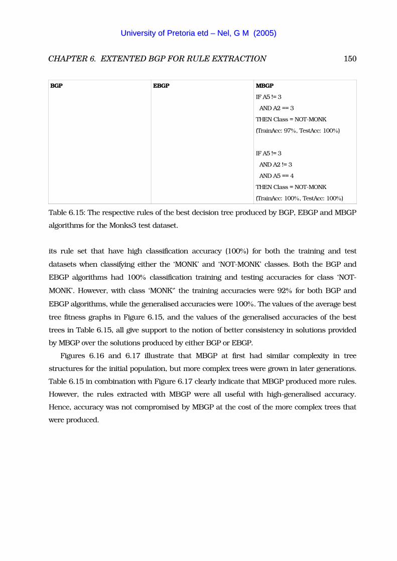
CHAPTER 6. EXTENTED BGP FOR RULE EXTRACTION 150
BGP EBGP MBGP
IF A5 != 3
AND A2 == 3
THEN Class = NOT-MONK
(TrainAcc: 97, TestAcc: 100)
IF A5 != 3
AND A2 != 3
AND A5 == 4
THEN Class = NOT-MONK
(TrainAcc: 100, TestAcc: 100)
Table 6.15: The respective rules of the best decision tree produced by BGP, EBGP and MBGP
algorithms for the Monks3 test dataset.
its rule set that have high classification accuracy (100) for both the training and test
datasets when classifying either the ‘MONK’ and ‘NOT-MONK’ classes. Both the BGP and
EBGP algorithms had 100 classification training and testing accuracies for class ‘NOT-
MONK’. However, with class ‘MONK‘’ the training accuracies were 92 for both BGP and
EBGP algorithms, while the generalised accuracies were 100. The values of the average best
tree fitness graphs in Figure 6.15, and the values of the generalised accuracies of the best
trees in Table 6.15, all give support to the notion of better consistency in solutions provided
by MBGP over the solutions produced by either BGP or EBGP.
Figures 6.16 and 6.17 illustrate that MBGP at first had similar complexity in tree
structures for the initial population, but more complex trees were grown in later generations.
Table 6.15 in combination with Figure 6.17 clearly indicate that MBGP produced more rules.
However, the rules extracted with MBGP were all useful with high-generalised accuracy.
Hence, accuracy was not compromised by MBGP at the cost of the more complex trees that
were produced.
UUnniivveerrssiittyy ooff PPrreettoorriiaa eettdd –– NNeell,, GG MM ((22000055))
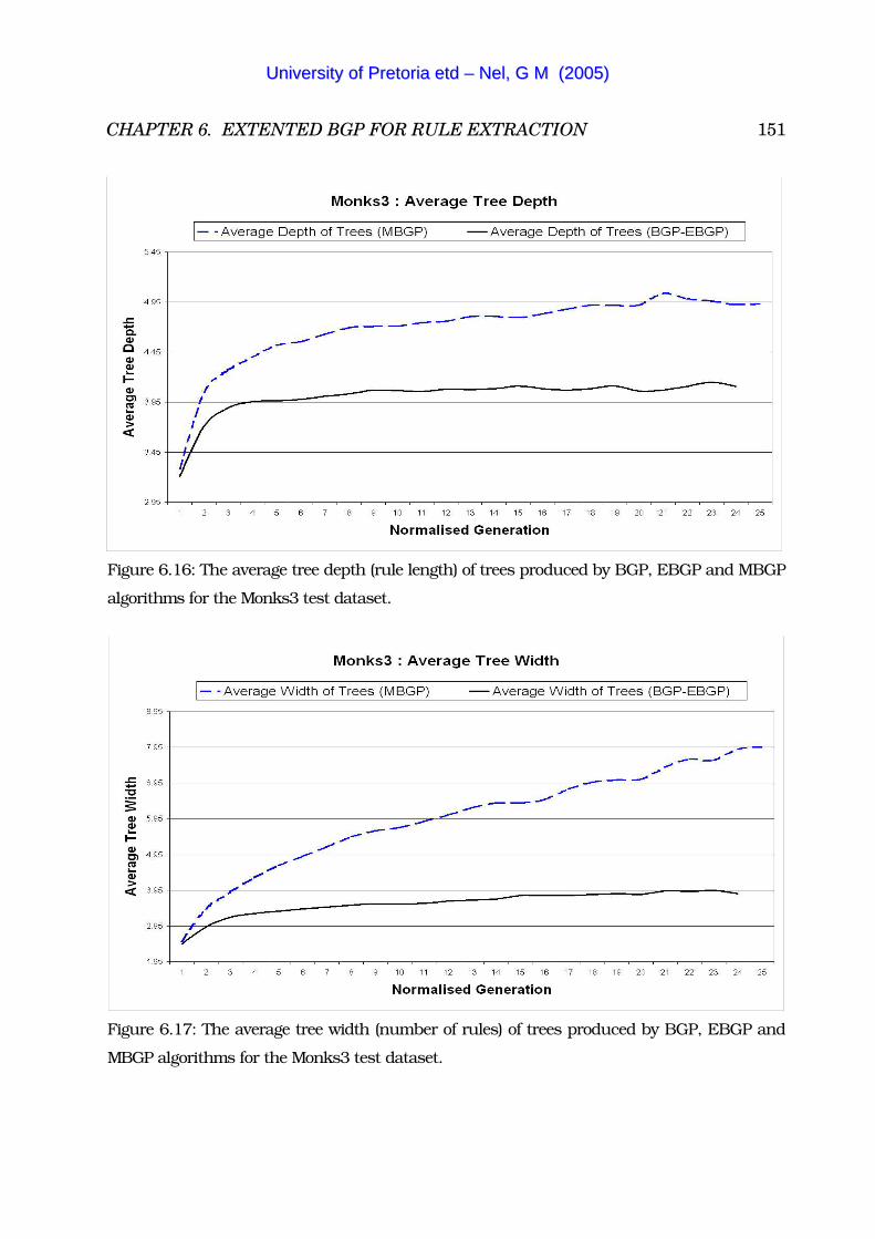
CHAPTER 6. EXTENTED BGP FOR RULE EXTRACTION 151
Figure 6.16: The average tree depth (rule length) of trees produced by BGP, EBGP and MBGP
algorithms for the Monks3 test dataset.
Figure 6.17: The average tree width (number of rules) of trees produced by BGP, EBGP and
MBGP algorithms for the Monks3 test dataset.
UUnniivveerrssiittyy ooff PPrreettoorriiaa eettdd –– NNeell,, GG MM ((22000055))
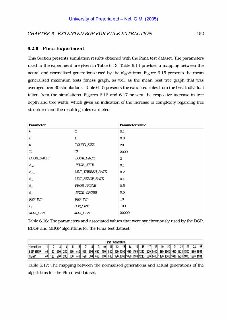
CHAPTER 6. EXTENTED BGP FOR RULE EXTRACTION 152
6.2.6 Pima Experiment
This Section presents simulation results obtained with the Pima test dataset. The parameters
used in the experiment are given in Table 6.13. Table 6.14 provides a mapping between the
actual and normalised generations used by the algorithms. Figure 6.15 presents the mean
generalised maximum tests fitness graph, as well as the mean best tree graph that was
averaged over 30 simulations. Table 6.15 presents the extracted rules from the best individual
taken from the simulations. Figures 6.16 and 6.17 present the respective increase in tree
depth and tree width, which gives an indication of the increase in complexity regarding tree
structures and the resulting rules extracted.
Parameter Parameter value
� C
L L
n TOURN_SIZE
T0 T0
LOOK_BACK LOOK_BACK
�attr PROB_ATTR
�thres MUT_THRESH_RATE
�rel MUT_RELOP_RATE
�p PROB_PRUNE
�r PROB_CROSS
REP_INT REP_INT
PT POP_SIZE
MAX_GEN MAX_GEN
0.1
0.0
20
2000
2
0.1
0.2
0.4
0.5
0.5
10
100
20000
Table 6.16: The parameters and associated values that were synchronously used by the BGP,
EBGP and MBGP algorithms for the Pima test dataset.
Table 6.17: The mapping between the normalised generations and actual generations of the
algorithms for the Pima test dataset.
UUnniivveerrssiittyy ooff PPrreettoorriiaa eettdd –– NNeell,, GG MM ((22000055))
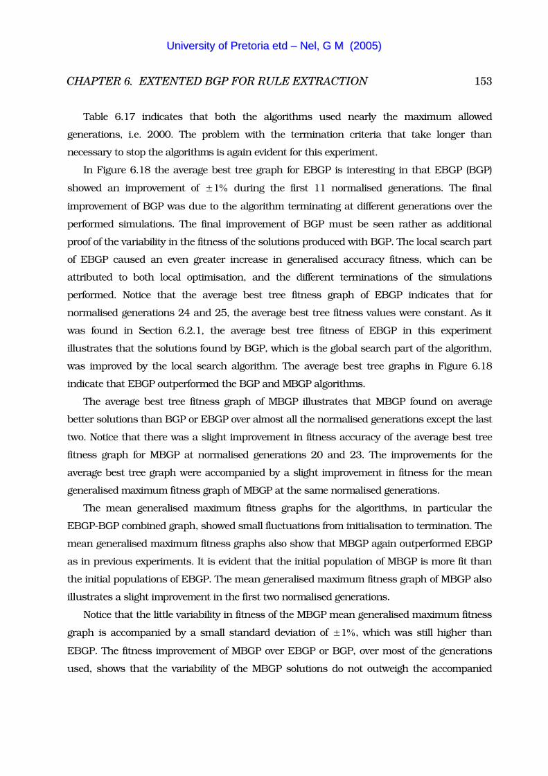
CHAPTER 6. EXTENTED BGP FOR RULE EXTRACTION 153
Table 6.17 indicates that both the algorithms used nearly the maximum allowed
generations, i.e. 2000. The problem with the termination criteria that take longer than
necessary to stop the algorithms is again evident for this experiment.
In Figure 6.18 the average best tree graph for EBGP is interesting in that EBGP (BGP)
showed an improvement of �1 during the first 11 normalised generations. The final
improvement of BGP was due to the algorithm terminating at different generations over the
performed simulations. The final improvement of BGP must be seen rather as additional
proof of the variability in the fitness of the solutions produced with BGP. The local search part
of EBGP caused an even greater increase in generalised accuracy fitness, which can be
attributed to both local optimisation, and the different terminations of the simulations
performed. Notice that the average best tree fitness graph of EBGP indicates that for
normalised generations 24 and 25, the average best tree fitness values were constant. As it
was found in Section 6.2.1, the average best tree fitness of EBGP in this experiment
illustrates that the solutions found by BGP, which is the global search part of the algorithm,
was improved by the local search algorithm. The average best tree graphs in Figure 6.18
indicate that EBGP outperformed the BGP and MBGP algorithms.
The average best tree fitness graph of MBGP illustrates that MBGP found on average
better solutions than BGP or EBGP over almost all the normalised generations except the last
two. Notice that there was a slight improvement in fitness accuracy of the average best tree
fitness graph for MBGP at normalised generations 20 and 23. The improvements for the
average best tree graph were accompanied by a slight improvement in fitness for the mean
generalised maximum fitness graph of MBGP at the same normalised generations.
The mean generalised maximum fitness graphs for the algorithms, in particular the
EBGP-BGP combined graph, showed small fluctuations from initialisation to termination. The
mean generalised maximum fitness graphs also show that MBGP again outperformed EBGP
as in previous experiments. It is evident that the initial population of MBGP is more fit than
the initial populations of EBGP. The mean generalised maximum fitness graph of MBGP also
illustrates a slight improvement in the first two normalised generations.
Notice that the little variability in fitness of the MBGP mean generalised maximum fitness
graph is accompanied by a small standard deviation of �1, which was still higher than
EBGP. The fitness improvement of MBGP over EBGP or BGP, over most of the generations
used, shows that the variability of the MBGP solutions do not outweigh the accompanied
UUnniivveerrssiittyy ooff PPrreettoorriiaa eettdd –– NNeell,, GG MM ((22000055))
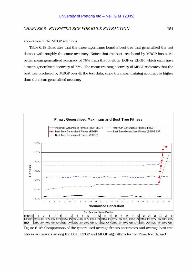
CHAPTER 6. EXTENTED BGP FOR RULE EXTRACTION 154
accuracies of the MBGP solutions.
Table 6.18 illustrates that the three algorithms found a best tree that generalised the test
dataset with roughly the same accuracy. Notice that the best tree found by MBGP has a 1
better mean generalised accuracy of 78 than that of either BGP or EBGP, which each have
a mean generalised accuracy of 77. The mean training accuracy of MBGP indicates that the
best tree produced by MBGP over-fit the test data, since the mean training accuracy is higher
than the mean generalised accuracy.
Figure 6.18: Comparisons of the generalised average fitness accuracies and average best tree
fitness accuracies among the BGP, EBGP and MBGP algorithms for the Pima test dataset.
UUnniivveerrssiittyy ooff PPrreettoorriiaa eettdd –– NNeell,, GG MM ((22000055))

CHAPTER 6. EXTENTED BGP FOR RULE EXTRACTION 155
BGP EBGP MBGP
Number of rules in tree: 4
The tree has depth: 3
The tree has width: 4
Accuracy on test set is: 77
Accuracy on training set is: 77
Rules:
IF a2 > 126
AND a6 > 30.000
THEN Class = POSITIVE
(TrainAcc: 68, TestAcc: 79)
IF a2 > 126
AND a6 <= 30.000
THEN Class = NEGATIVE
(TrainAcc: 70, TestAcc: 73)
IF a2 <= 126
AND a8 != 54
THEN Class = NEGATIVE
(TrainAcc: 82, TestAcc: 77)
IF a2 <= 126
AND a8 == 54
THEN Class = POSITIVE
(TrainAcc: 67, TestAcc: 0)
Number of rules in tree: 4
The tree has depth: 4
The tree has width: 2
Accuracy on test set is: 77
Accuracy on training set is: 77
Rules:
IF a6 <= 30.300
THEN Class = NEGATIVE
(TrainAcc: 83, TestAcc: 79)
IF a6 > 30.300
AND a2 < 128
THEN Class = NEGATIVE
(TrainAcc: 76, TestAcc: 71)
IF a6 > 30.300
AND a2 >= 128
AND a7 >= 0.740
THEN Class = POSITIVE
(TrainAcc: 85, TestAcc: 82)
IF a6 > 30.300
AND a2 >= 128
AND a7 < 0.740
THEN Class = POSITIVE
(TrainAcc: 65, TestAcc: 78)
Number of rules in tree: 6
The tree has depth: 5
The tree has width: 4
Accuracy on test set is: 78
Accuracy on training set is: 79
Rules:
IF a2 < 112
THEN Class = NEGATIVE
(TrainAcc: 87, TestAcc: 84)
IF a2 >= 112
AND a6 >= 30.000
AND a2 < 166
AND a8 < 31
THEN Class = NEGATIVE
(TrainAcc: 68, TestAcc: 60)
IF a2 >= 112
AND a6 >= 30.000
AND a2 < 166
AND a8 >= 31
THEN Class = POSITIVE
(TrainAcc: 70, TestAcc: 74)
IF a2 >= 112
AND a6 >= 30.000
AND a2 >= 166
THEN Class = POSITIVE
(TrainAcc: 88, TestAcc: 90)
(continued ...)
UUnniivveerrssiittyy ooff PPrreettoorriiaa eettdd –– NNeell,, GG MM ((22000055))
CHAPTER 6. EXTENTED BGP FOR RULE EXTRACTION 156
BGP EBGP MBGP
IF a2 >= 112
AND a6 < 30.000
AND a8 != 36
THEN Class = NEGATIVE
(TrainAcc: 74, TestAcc: 74)
IF a2 >= 112
AND a6 < 30.000
AND a8 == 36
THEN Class = POSITIVE
(TrainAcc: 67, TestAcc: 0)
Table 6.18: The respective rules of the best decision tree produced by BGP, EBGP and MBGP
algorithms for the Pima test dataset.
When the individual rules produced by the three algorithms are examined, it becomes
clear that there are some rules in each of the three rule sets which over-fit the test dataset. All
these rules have higher training accuracies than the accompanied generalised accuracies.
BGP and MBGP seems to have produced a best tree that over-fit the tests data. In fact, both
the BGP and MBGP best trees contains some rules that are over-fitting the test data, while
other rules exist in the same rule set that are extremely accurate and which do not over-fit the
test data. Note that the best tree found by MBGP even has a rule that is ‘useless’ since it does
not classify one instance of class ‘POSITIVE’. The best rule founded by MBGP, which
classifies class ‘POSITIVE’, does so with a generalised accuracy of 90 without over-fitting
the test dataset. The best rules that BGP or EBGP extracted to classify class ‘POSITIVE’ has
generalised accuracies of 79 and 82 respectively. However, note that the rule produced by
EBGP that classifies class ‘POSITIVE’ is over-fitting the test dataset. The second best rule in
terms of generalised accuracy for class ‘POSITIVE’ produced by EBGP has a generalised
accuracy of 78. For class ‘NEGATIVE’ the generalised accuracy for the best rule produced
by BGP, EBGP and MBGP are 77, 79 and 84 respectively. Notice that the three best
rules for class ‘NEGATIVE’ are over-fitting the test dataset for each of the three algorithms.
BGP and MBGP each produced an additional rule to classify class ‘NEGATIVE’, which has
respective accuracies of 73 and 74, while EBGP had no rule that did not over-fit class
UUnniivveerrssiittyy ooff PPrreettoorriiaa eettdd –– NNeell,, GG MM ((22000055))
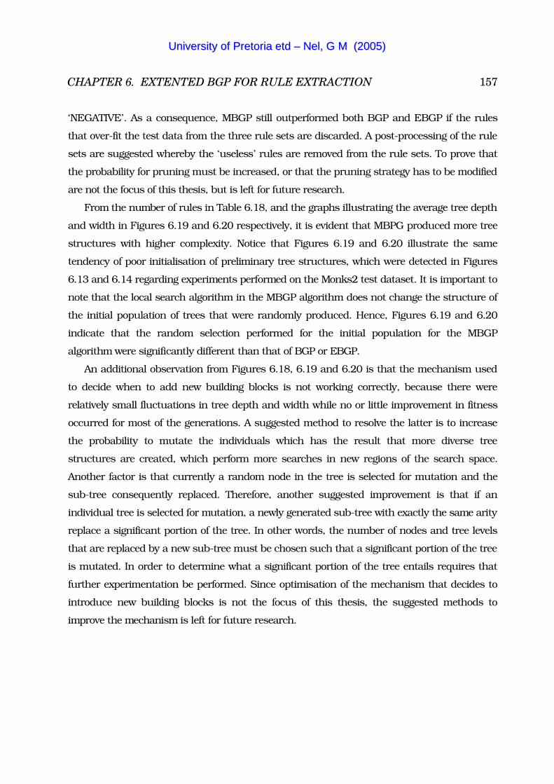
CHAPTER 6. EXTENTED BGP FOR RULE EXTRACTION 157
‘NEGATIVE’. As a consequence, MBGP still outperformed both BGP and EBGP if the rules
that over-fit the test data from the three rule sets are discarded. A post-processing of the rule
sets are suggested whereby the ‘useless’ rules are removed from the rule sets. To prove that
the probability for pruning must be increased, or that the pruning strategy has to be modified
are not the focus of this thesis, but is left for future research.
From the number of rules in Table 6.18, and the graphs illustrating the average tree depth
and width in Figures 6.19 and 6.20 respectively, it is evident that MBPG produced more tree
structures with higher complexity. Notice that Figures 6.19 and 6.20 illustrate the same
tendency of poor initialisation of preliminary tree structures, which were detected in Figures
6.13 and 6.14 regarding experiments performed on the Monks2 test dataset. It is important to
note that the local search algorithm in the MBGP algorithm does not change the structure of
the initial population of trees that were randomly produced. Hence, Figures 6.19 and 6.20
indicate that the random selection performed for the initial population for the MBGP
algorithm were significantly different than that of BGP or EBGP.
An additional observation from Figures 6.18, 6.19 and 6.20 is that the mechanism used
to decide when to add new building blocks is not working correctly, because there were
relatively small fluctuations in tree depth and width while no or little improvement in fitness
occurred for most of the generations. A suggested method to resolve the latter is to increase
the probability to mutate the individuals which has the result that more diverse tree
structures are created, which perform more searches in new regions of the search space.
Another factor is that currently a random node in the tree is selected for mutation and the
sub-tree consequently replaced. Therefore, another suggested improvement is that if an
individual tree is selected for mutation, a newly generated sub-tree with exactly the same arity
replace a significant portion of the tree. In other words, the number of nodes and tree levels
that are replaced by a new sub-tree must be chosen such that a significant portion of the tree
is mutated. In order to determine what a significant portion of the tree entails requires that
further experimentation be performed. Since optimisation of the mechanism that decides to
introduce new building blocks is not the focus of this thesis, the suggested methods to
improve the mechanism is left for future research.
UUnniivveerrssiittyy ooff PPrreettoorriiaa eettdd –– NNeell,, GG MM ((22000055))
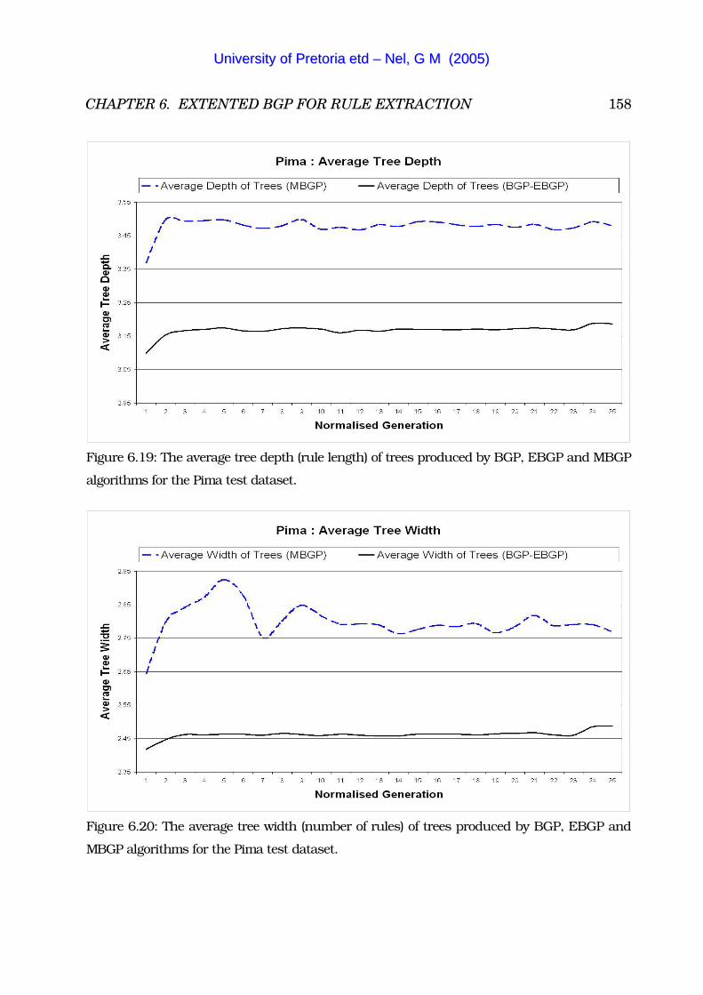
CHAPTER 6. EXTENTED BGP FOR RULE EXTRACTION 158
Figure 6.19: The average tree depth (rule length) of trees produced by BGP, EBGP and MBGP
algorithms for the Pima test dataset.
Figure 6.20: The average tree width (number of rules) of trees produced by BGP, EBGP and
MBGP algorithms for the Pima test dataset.
UUnniivveerrssiittyy ooff PPrreettoorriiaa eettdd –– NNeell,, GG MM ((22000055))
CHAPTER 6. EXTENTED BGP FOR RULE EXTRACTION 159
6.2.7 Combined Observations from Experiments
The combined observations from the experimental results are now discussed, and from these
observations some conclusions are drawn and presented in Chapter 7. Note that the BGP
algorithm was used as the base for comparing all results. Some important aspects regarding
the experimental results with the BGP, EBGP and MBGP algorithms, were identified and are
discussed in this Section. The first result discussed pertains to the difference in the number
of generations required by the three algorithms to find a solution and terminate. Thereafter,
the results that compare the performance of the EBGP algorithm to the standard BGP
algorithm are discussed. The comparative results for the MBGP algorithm with both BGP and
EBGP are finally discussed.
The three algorithms used essentially the same number of generations to complete and
produce a solution over four of the experiments. The two exceptions were the Monks1 and
Monks3 experiments. Monks3 was the only algorithm where the MBGP algorithm used
substantially more generations (�10) in finding a solution. The Monks1 experiment showed
a substantial difference in the number of generations used by the algorithms, which suggests
a problem with the termination condition used. The notion that there is a problem with the
termination criteria is supported by the fact that in all experiments, with the exception of
Monks1, the algorithms used nearly the maximum allowed generations (T0 parameter) to find
solutions, while little or no improvement in fitness occurred.
Note that BGP and EBGP are essentially the same algorithm. The only difference is that
EBGP tries to refine the solution found by the standard BGP algorithm. Hence, EBGP and
BGP figures were shown mainly to be the same, with improvements brought on by local
optimisations (EBGP) clearly indicated in the figures.
The next few observations are made regarding the performance of the EBGP algorithm as
compared with the standard BGP algorithm. The combined average best tree fitness graphs of
BGP and EBGP indicate the average fitness of the best solutions over 30 simulations. If the
solution found by the global search part of the EBGP algorithm can be refined further by the
local search part, then the improvement will be evident in the combined average best tree
fitness graph of BGP and EBGP. The EBGP algorithm was successful with the Iono and Pima
test datasets, while no refinement of the solutions found by standard BGP was evident in the
remaining experiments.
UUnniivveerrssiittyy ooff PPrreettoorriiaa eettdd –– NNeell,, GG MM ((22000055))
CHAPTER 6. EXTENTED BGP FOR RULE EXTRACTION 160
A prominent aspect of the combined average best tree graph of EBGP and BGP over all the
experimental simulations performed is that the graph does not show any significant increase
in fitness value for most of the normalised generations. The same trend is detected in the
combined EBGP and BGP mean generalised maximum fitness graph, which indicates that
the mechanism for introducing new building blocks is not operating as intended.
The combined EBGP and BGP mean generalised maximum fitness graph supported the
notion that local search refinement was responsible for improvements of the solutions
produced during the Iono and Pima experiments. The combined mean generalised maximum
fitness graph of EBGP and BGP did not improve significantly as had the combined average
best tree fitness graph in the final few normalised generations. The results of the Table with
the best tree found for each of the algorithms provides further support for the statement.
The standard deviation on solutions as found by EBGP and BGP indicates that both
algorithms produced solutions that deviated little from the average solution. It can be seen
from the combined average tree depth and width graph for EBGP and BGP that there was
seldom an increase in the complexity of either the EBGP and BGP tree structures. This little
variation in solutions, coupled with the small increases in tree structure complexities,
confirms the notion that the mechanism that introduces new building blocks was not
working well.
The following result discussion compares the MBGP algorithm with the BGP and EBGP
algorithms. From all the figures for all the tests performed, the first observation is that the
initial starting fitness values of all the graphs representing results obtained with the MBGP
algorithm are always higher than the starting fitness values of the graphs representing
simulations performed with EBGP and BGP. The local optimisation of the initial population in
the starting generation is responsible for the improvement of fitness that MBGP obtained. The
local optimisation is performed on the initial population to ensure that the building blocks
used to build solutions are optimal. A guarantee can therefore be given that all building
blocks are locally optimised.
The average best tree fitness graphs for MBGP over all the experiments supports the
notion that MBGP produced building blocks that were more accurate, which in turn allowed
the evolutionary operators to work more efficiently. In fact, from all the mean generalised
maximum fitness and the average best tree fitness graphs for MBGP, another important
observation is that the MBGP algorithm can terminate sooner. The earlier termination can be
UUnniivveerrssiittyy ooff PPrreettoorriiaa eettdd –– NNeell,, GG MM ((22000055))

CHAPTER 6. EXTENTED BGP FOR RULE EXTRACTION 161
achieved because the mean population accuracy for MBGP was improved substantially only
in the first few generations. Subsequent improvements in accuracy were in fact not
substantial after the first half of the normalised generations were used. As a consequence
MBGP could terminate in all of the experiments before half the normalised generations had
been used.
The respective fitness values for all the MBGP graphs over all the experiments were
substantially higher than the fitness values achieved by either EBGP or BGP. The only
exception was the final fitness values produced in the last normalised generation of the Pima
experiment by the average best tree graphs of BGP and EBGP, which were better by 0.5
and 2 respectively.
Both the mean generalised maximum fitness graphs and the average best tree fitness
graphs from all the experiments indicate that MBGP on average produced populations with
higher generalised accuracies. The Monks2 and Pima test datasets were the only experiments
where MBGP produced solutions as indicated by both the mean generalised maximum
fitness graphs and the average best tree fitness graphs that did not improve the fitness of the
graphs of BGP and EBGP by more than 10. However, notice that the MBGP algorithm still
produced solutions that were better or equivalent in fitness for the Monks2 and Pima
experiments. Coincidently, the Monks2 and Pima experiments showed that the initialisation
of the initial populations for MBGP algorithm did not produce initial individuals (tree
structures) with similar complexities as had those initial individuals produced for the EBGP
and BGP combination. The average tree width graphs and the average tree depth graphs
confirmed for the two experimental cases that the structures for the initial trees for MBGP
were more complex than those of EBGP (BGP). Since the local search algorithm used with
MBGP refines the solutions, and does not add more branches or more hierarchical levels to
the tree structures, it is evident that the process that initialised the populations did so
ineffectively. Random initialisation and ineffective adjustments were the cause for the poor
initialisation of the population.
The mean generalised maximum fitness graphs of MBGP over all the experiments
indicated another tendency, which is that the fitness always improved over the normalised
generations, while the fitness of the combined mean generalised maximum fitness graphs for
EBGP and BGP did not. Remember that the parameters were chosen the same
(synchronised) for the different algorithms. Therefore, the only explanation for the
UUnniivveerrssiittyy ooff PPrreettoorriiaa eettdd –– NNeell,, GG MM ((22000055))
CHAPTER 6. EXTENTED BGP FOR RULE EXTRACTION 162
improvement over the normalised generations of MBGP is that the evolutionary operators
were operating better by using locally optimised building blocks. It is also evident that MBGP
was less prone than BGP and EBGP to a failure in the mechanism that introduced new
building blocks.
Another observation can be made when the generalised fitness values of the best tree
found for the three algorithms given in the Tables are compared with the highest fitness value
reached by the respective average best tree fitness graphs in each of the experiments. Except
for Monks2 the fitness values of the MBGP average best tree fitness graphs are closer to the
generalised fitness values of the best tree Table. With regard to the smaller difference in the
respective fitness values of MBGP, the implication is that MBGP on average produces
solutions that are more consistent in generalised accuracies. In other words, over the
simulations that were performed per experiment, MBGP produced on average best solutions
that were closer to the best solution that was found over the simulations rather than either
BGP or EBGP.
A pertinent aspect of the MBGP results is that in all experiments conducted the standard
deviation of the solutions found by MBGP is much higher than that of the combined results
for BGP and EBGP. Only in the Pima experiment was the standard deviation on average
higher by a small amount than the combined standard deviation of EBGP and BGP. Note that
the standard deviation gives an indication of the dependability of the algorithm. Incidentally,
MBGP showed in the Pima experiment the least amount of fitness improvement in the mean
generalised maximum fitness over the generations. When considering the increased standard
deviation of MBGP along with the higher average fitness shown by the mean generalised
maximum fitness graphs, it becomes clear that there was a small subset of individuals in the
population of MBGP that were less fit than the average individuals in the population. For the
BGP and EBGP combination there were even fewer individuals in the subset of less fit
individuals that caused the increase in standard deviation. It is important to note that even
though the standard deviation for MBGP was higher in all experiments than the BGP and
EBGP combination, the average accuracy of the solutions found by MBGP exceeded that of
those found by the EBGP-BGP combination. In certain experiments the improvements in
accuracy made by MBGP over EBGP were substantially greater than the standard deviation
differences.
Further analysis of the Tables that contain the best tree found over the test datasets
UUnniivveerrssiittyy ooff PPrreettoorriiaa eettdd –– NNeell,, GG MM ((22000055))
CHAPTER 6. EXTENTED BGP FOR RULE EXTRACTION 163
showed that MBGP on average extracted more rules than BGP or EBGP. The graphs
indicating the average tree width and average tree depth supported the notion that MBGP
produced more complex tree structures from which more rules were extracted with higher
associated complexity. The rules extracted with MBGP with increased complexities had less of
a tendency to over-fit the data when compared with the rules produced by BGP or EBGP.
Hence, complexity was introduced though not at the cost of accuracy. In fact, accuracy for all
the experiments was significantly improved. When a post-selection of the best rules in the
rule set for each experiment was performed, it became evident that the MBGP rules
generalised the data better and were better able to discern (refine the boundaries) of each of
the classes in a test dataset. One problem that MBGP had experienced was that ‘useless’
rules, which did not classify any class instances of the validation set, were extracted from the
best tree as part of the set of highly accurate rules. Note that these ‘useless’ rules also over-fit
the data by having high accuracies on the training dataset. Note that the rule sets extracted
by MBGP were equal to, or more accurate than the rule sets extracted by BGP or EBGP. As a
consequence the pruning operation commonly used by the three algorithms had become
suspect of being ineffective in removing the less significant parts of the trees in the
populations.
6.3 Concluding Remarks
In this Chapter two methods were evaluated for extending the standard BGP algorithm with a
local search algorithm against the original BGP algorithm. The EBGP algorithm offered a
simple refinement of the solution found by the BGP global search algorithm. MBGP
introduced local search as an additional operator that is used by the standard BGP algorithm.
The experimental results gathered on six different test datasets were provided in Figures and
Tables, and each experiment was individually discussed in Sections 6.2.1 to 6.2.6. Section
6.2.7 gave combined observations regarding the experimental results. The following Chapter
concludes this thesis by summarising the conclusions drawn from the present Chapter and
suggests further research possibilities.
UUnniivveerrssiittyy ooff PPrreettoorriiaa eettdd –– NNeell,, GG MM ((22000055))
Chapter 7
Conclusion
7.1 Conclusion and Summary
This study investigated in two specific ways the effectiveness and efficiency of combining a
global search algorithm with a local search algorithm. As a result two new algorithms were
developed for rule extraction. Note that the newly developed algorithms provided in this thesis
were not tested against a complex, real-world optimisation problem.
Chapter 3 presented an overview of the building block approach to genetic programming
for rule extraction algorithm (BGP). It appeared that the fitness function of the standard BGP
algorithm could be improved. Therefore, a new fitness function was proposed. Experimental
results in Section 4.4 indicated that fitness improvements by the newly proposed fitness
function were not substantial enough over the fitness resulting from the original fitness
function. Hence, the fitness function of the standard BGP algorithm as provided by
Rouwhorst [69] was used in further experiments.
Chapter 5 introduced a newly developed local search method, namely the directed
increasing incremental local search (DIILS), which was combined with the standard BGP
algorithm to produce two new algorithms. With the first algorithm local search is used to
refine the solution found by the standard BGP algorithm. Therefore the first algorithm is
referred to as the ‘Enhanced Building Block Approach to Genetic Programming’ (EBGP)
algorithm. With the second algorithm local search is combined as an operand in the standard
BGP algorithm in order to create the ‘Memetic Building Block Approach to Genetic
164
UUnniivveerrssiittyy ooff PPrreettoorriiaa eettdd –– NNeell,, GG MM ((22000055))
CHAPTER 7. CONCLUSION 165
Programming’ (MBGP) algorithm. Hence, the EBGP algorithm refines only the solution
provided by the standard BGP algorithm, while MBGP actively refines all possible solutions
produced by the initial random selection process, as well those solutions produced during the
evolutionary process.
It was found that EBGP did improve in some of the experiments on the standard BGP
algorithm, but was not nearly as successful as MBGP. The standard deviation of the EBGP
algorithm was not different from that of the original BGP algorithm, because the global search
part of EBGP used the BGP algorithm. Once BGP had found a solution, it was optimised
locally by EBGP. As a consequence the EBGP algorithm improved the solution of two of the
experiments without a decrease in reliability of the solutions found. In all experiments
performed, the additional computational complexity introduced by the EBGP algorithm over
that of the standard BGP algorithm was negligible.
A problem was shown to exist in the mechanism that introduces new building blocks for
both the BGP and EBGP algorithms, because either very small or no improvements in the
fitness function values over most of the generations occurred in all the experiments
performed. The associated complexity in the structures of the individuals was not increased
when the fitness improvements were small for BGP and EBGP. The constant complexity in
the structures of the individuals confirmed the suspicion that new building blocks had not
been added at appropriate times. MBGP achieved greater improvements over the generations
while the complexity of the structures of the individuals increased.
In all experiments the MBGP algorithm showed improvement over both the standard BGP
and EBGP algorithms. Note that there was found to be a significant difference between a
memetic algorithm (MBGP) and a global search algorithm extended with a local search
method (EBGP). A memetic algorithm is implemented in a specific manner where local search
is employed as an additional operator. Note that a memetic algorithm is not a global search
algorithm that happens to perform local search as an additional operation. The direct
comparison between standard BGP, EBGP and the MBGP algorithms indicated that the
memetic algorithm achieved an improved performance by the evolutionary operators during
the evolutionary search process. Note that with improved performance we mean that the
accuracy of solutions produced was better. Better accuracy came with a trade-off in
computational time complexity. The MBGP algorithm required fewer generations to optimise a
solution with high accuracy. The solutions produced by MBGP were more complex than that
UUnniivveerrssiittyy ooff PPrreettoorriiaa eettdd –– NNeell,, GG MM ((22000055))
CHAPTER 7. CONCLUSION 166
of BGP or EBGP, but the associated accuracies of the MBGP solutions were significantly
higher than the solutions produced by the others. Consequently, the increase in the
complexity of the structure of solutions was not obtained at the cost of accuracies of the
solutions.
The higher fitness of the initial population of the MBGP algorithm, combined with the
improved evolutionary process shown by MBGP, provides experimental proof that the
building block hypothesis (BBH) is flawed. This is so because the BBH assumes that the
building blocks used have the best possible fitness during the optimisation process of
solutions. Furthermore, the BBH assumes that a constant fitness is maintained by the
building blocks, even when the evolutionary operators change the individuals (solutions) in a
population. A suggested extension to the BBH is to include an additional check that will
ensure that the building blocks used are at all times optimal. Note that the MBGP algorithm
can guarantee that all building blocks used during the search process are at all times locally
optimal.
Three disadvantages were identified with the MBGP algorithm.
� In order to produce a solution, the computation time taken by MBGP was much longer
than that taken by either BGP or EBGP. The local search algorithm is directly responsible
for the increased computation times for the MBGP algorithm, but the number of
generations it took to produce a solution of higher accuracy than either BGP or EBGP were
significantly less. The smaller number of generations used is clearly illustrated by the
higher fitness in the average best tree graphs as seen in Figures 6.3, 6.6, 6.12 and 6.14.
� The complexity of rules extracted from the best decision trees as provided by MBGP were
constantly higher than the complexity of those extracted using the BGP and EBGP
algorithms. As a consequence of the increased complexity of the solutions produced by
MBGP, a higher number of rules were extracted with MBGP rather than the number of
rules extracted with either BGP or EBGP. One of the objectives of rule extraction is to
produce as few rules as possible. However, the rules extracted with MBGP were able to
better define the class boundaries of all the classes in the testing problems, hence those
extracted had higher accuracies.
� The standard deviation of the population of solutions produced by MBGP was significantly
higher over the generations than that of either BGP or EBGP.
UUnniivveerrssiittyy ooff PPrreettoorriiaa eettdd –– NNeell,, GG MM ((22000055))
CHAPTER 7. CONCLUSION 167
Some common problems were detected that are shared by the three algorithms. The
termination condition used by the three algorithms was found to be inefficient and unable to
terminate when no improvement in the fitness of the populations occurred. The initialisation
method whereby the population of individuals in the first generation is initialised was found
to be unreliable. The mechanism that decides when to add new building blocks was found to
be ineffective. Rules that did not classify any class instances were extracted as part of the rule
set of highly accurate rules, which indicated that there is a problem with the pruning
operation.
7.2 Future Research
Several areas are identified for future research on the improvement of MBGP, EBGP and BGP
performance.
Improve the random population initialiser for the algorithms.
The initialisation of the individuals in the first generation of a population for the tested
algorithms has indicated differences in structural complexities of the individuals. The
complexities in the structures of the initial populations for the algorithms must be equivalent
to ensure that all the algorithms initially use the simplest building blocks. Hence, a new
initialisation procedure is required. A suggested method is to build the initial population by
selecting for each individual a building block such that the individual is valid and consists of
only the selected building block.
Improve termination criteria used by BGP, EBGP and MBGP.
The termination criteria for the algorithms can be improved by terminating the algorithm if
the fitness of the population of solutions does not improve for several generations, which
consequently will cause reduction in the time to produce a solution.
Improving the mechanism which introduces new building blocks.
A suggestion to improve the mechanism that decides to add new building blocks is to
increase the probability of mutating the individuals so that more are chosen for mutation by
UUnniivveerrssiittyy ooff PPrreettoorriiaa eettdd –– NNeell,, GG MM ((22000055))
CHAPTER 7. CONCLUSION 168
adding new building blocks. Another suggestion is to replace large portions of the individual
that was selected for mutation with new building blocks that do not increase the complexity
of the structure of the individual. Some experimentation is required in order to determine the
ideal size of the portions to be replaced.
Improving the pruning operator.
The suggestions to improve the pruning operator are to either increase the probability with
which pruning are performed, or to use a stricter criterion to prune only those structures in
an individual (branches in a decision tree) from which inaccurate rules are extracted.
Optimisation of MBGP input parameters.
The optimal parameter values for each experiment were first determined for the standard
BGP algorithm. The input parameters used by the MBGP algorithm were thereafter
intentionally chosen as being the same as the parameters for the standard BGP algorithm.
The result is that the direct performance was determined of the improvement of the MBGP
algorithm over the standard BGP algorithm. Hence, direct comparisons of the MBGP, EBGP
and standard BGP algorithms were possible. However, the best performance gain was not
determined for that which might be achievable with optimised parameter settings for MBGP.
Therefore, an additional investigation is required to determine whether the optimisation of the
parameters for the MBGP algorithm will address the disadvantages of a higher standard
deviation that was observed and the greater number of rules extracted with the MBGP
algorithm.
Influence of a different local optimisation algorithm on MBGP performance.
In terms of the computational complexity and performance of the MBGP algorithm, the
difference between the current local optimisation algorithm (DIILS) and a different local
optimisation algorithm requires further research.
Determine effectiveness and efficiency of MBGP with large datasets andcomplex, real-world problems.
The newly developed algorithms presented in this thesis were not tested against a large
UUnniivveerrssiittyy ooff PPrreettoorriiaa eettdd –– NNeell,, GG MM ((22000055))

CHAPTER 7. CONCLUSION 169
database or utilised in solving a complex, real-world optimisation problem. Hence, additional
research is required whereby the new algorithms are further tested in those scenarios.
UUnniivveerrssiittyy ooff PPrreettoorriiaa eettdd –– NNeell,, GG MM ((22000055))
Bibliography
[1] E. H. L. Aarts, J. Korst, Simulated Annealing and Boltzmann Machines: A Stochastic
Approach to combinatorial optimization and Neural computing, John Wiley & Sons Ltd,
1989.
[2] R. Agrawal et al., Fast discovery of association rules, In: Advances in Knowledge
Discovery & Data Mining, UM. Fayyad et al. (Eds.), AAAI Press, Menlo Park, pages 307 –
328, 1996.
[3] T. Bäck, Evolutionary Algorithms in Theory and Practice., Oxford University Press, New
York, USA, 1996.
[4] T. Bäck, D. B. Fogel, and T. Michalewicz, editors, Basic Algorithms and Operators.,
volume 1 of Evolutionary Computation., Institute of Physics Publishing, Bristol and
Philidelphia, 1999.
[5] T. T. Bihn, U. Korn, Multi-criteria Control System Design Using an Intelligent Evolution
Strategy with Dynamical Constraints Boundaries., Institute of Automation, University
of Magdeburg, Germany, 1997.
[6] H. K. Birru, K. Chellapilla, R Sathyanarayan, Local Search Operators in Fast
Evolutionary Programming., IEEE Press, pages 1506 – 1513, 1999.
[7] H. K. Birru, K. Chellapilla, R. Sathyanarayan, Effectiveness of Local Search Operators in
Evolutionary Programming., Genetic Programming 98, Madison, WI, pages 753-761,
170
UUnniivveerrssiittyy ooff PPrreettoorriiaa eettdd –– NNeell,, GG MM ((22000055))
BIBLIOGRAPHY 171
1998.
[8] C. L. Blake, C. J. Merz, UCI Repository of machine learning databases, University of
California, Irvine, Dept. of Information and Computer Sciences,
‘http://www.ics.uci.edu/~mlearn/MLRepository.html’, September 2004, 1998.
[9] F. Boscheti, M. C. Dentith, R. D. List, Inversion of seismic refraction data using genetic
algorithms., Geophysics,volume 61, number 6, pages 1715 - 1727, 1996.
[10] R. Brits, Niching strategies for particle swarm optimization., Submitted M.Sc. thesis,
University of Pretoria, Pretoria, 2002.
[11] C. J. Burgess, A. G. Chalmers, The Optimisation of Irregular Multiprocessor Computer
Architectures using Genetic Algorithms., Baltzer Journals, August 2, 1999.
[12] E. Cant-Paz, C. Kamath, On the Use of Evolutionary Algorithms in Data mining.,
Published in ‘Data Mining: A Heuristic Approach’., Idea Group Publishing, 2001.
[13] M. J. Cavaretta, K. Chellapilla, Data Mining using Genetic Programming: The
Implications of Parsimony on Generalization Error., In Proceedings of the 1999
Congress on Evolutionary Computation, pages 1330 - 1337, IEEE-press, 1999.
[14] P. Cheeseman, M. Self, J. Kelly, J. Stutz, W. Taylor, D. Freeman, Bayesian
Classification., In Proceedings of American Association of Artificial Intelligence (AAAI), 7th
Annual Conference on A.I., pages 607 - 611, Morgan Kaufmann, 1988.
[15] K. Chellapilla, Evolving Computer Programs Without Subtree Crossover, IEEE
Transactions on Evolutionary Computation, volume 1, number 3, pages 209 - 216, 1997.
[16] L. Chen, Z. Qin, J. S. Liu, Exploring Hybrid Monte Carlo in Bayesian Computation., In
Proceedings ISBA 2000, ISBA and Eurostat, 2000.
[17] P. Clark, T. Niblett, The CN2 Induction Algorithm, Machine Learning, pages 261 – 283,
UUnniivveerrssiittyy ooff PPrreettoorriiaa eettdd –– NNeell,, GG MM ((22000055))
BIBLIOGRAPHY 172
1989.
[18] C. A. Coella, A Comprehensive Survey of Evolutionary-Based Multi-objective
Optimization Techniques., Laboratorio Nacional de Informatica Avanzada, Xalapa,
Veracruz, México, Engineering Design Centre, University of Plymouth, Plymouth, UK,
1999.
[19] C. A. Coella, A. D. Christiansen, Multi-objective Optimization of Trusses using Genetic
Algorithms., Engineering Design Centre, University of Plymouth, Plymouth, UK.
[20] C. Cotta, E. Alba, J. M. Troya, Stochastic Reverse Hillclimbing and Iterated Local
Search., IEEE Press, pages 1558 - 1565, 1999.
[21] C. R. Darwin, On the Origin of Species by Means of Natural Selection or the
Preservation of Favoured Races in the Struggle for Life., Murray, London, 1859.
[22] L. Davis, Applying Adaptive Algorithms to Epistatic Domains. In Proceedings of the
International Joint Conference on Artificial Intelligence, pages 162 - 164, 1985.
[23] R. Dawkins, The Selfish Gene., Oxford University Press, 1990.
[24] I. De Falco, A. Della Cioppa, E. Tarantino, Discovering interesting classification rules
with genetic programming., Applied Soft Computing, Elsevier Science Publishing,
Amsterdam, pages 257 - 269, 2002.
[25] J. Denzinger, T. Offermann, On Cooperation between Evolutionary Algorithms and
other Search Paradigms., IEEE Press, pages 2317 – 2324, 1999.
[26] R. Eberhart, P. Simpson, R. Dobbins, Computational Intelligence PC tools., AP
Professional, 1996.
[27] L. J. Eshelman, J. D. Schaffer, Real-coded genetic algorithms and interval schemata., In
UUnniivveerrssiittyy ooff PPrreettoorriiaa eettdd –– NNeell,, GG MM ((22000055))
BIBLIOGRAPHY 173
Foundations of Genetic Algorithm II, pages 187 - 202, Morgan Kaufmann, San Mateo,
CA, USA, 1990.
[28] S. Forrest, M. Mitchell, Relative Building-block Fitness and the Building-block
Hypothesis., In Foundations of Genetic Algorithms II, Morgan Kaufmann, San Mateo,
CA, 1993.
[29] J. M. Garibaldi, E. C. Ifeachor, Application of Simulated Annealing Fuzzy Model Tuning
to Umbilical Cord Acid-Base Interpretation, IEEE-FS Transactions On Fuzzy Systems,
Vol. 7, No. 1, page 72, February 1999
[30] D. E. Goldberg, Genetic Algorithms in Search, Optimization and Machine Learning.,
Addison-Wesley, MA, 1989.
[31] D. E. Goldberg, S Voessner, Optimizing global-local search hybrids., In GECCO'99
volume 1, pages 220 - 228, Morgan Kaufmann, San Francisco, 1999.
[32] M. Gorges-Schleuter, ASPARAGOS: An Asynchronous Parallel Genetic Optimization
Strategy., In Proceedings of the Third International Conference on Genetic Algorithms,
pages 422 - 427, Mogan Kaufmann, 1989.
[33] R. Hanson, J. Stutz, P. Cheeseman, Bayesian Classification with Correlation and
Inheritance., In Proceedings of the 12th International Joint Conference on Artificial
Intelligence, Sydney, Australia, August, pages 692 – 698, Morgan Kaufmann, 1991.
[34] R. Hanson, J. Stutz, P. Cheeseman, Bayesian Classification Theory., In Technical Report
FIA-90-12-7-01, NASA Ames Research Center, Artificial Intelligence Branch, May, 1991.
[35] R. J. W. Hodgson., Memetic Algorithms and the Molecular Geometry Optimisation
Problem., In Proceedings of the 2000 Congress on Evolutionary Computation (CEC2000),
San Diego, CA., pages 625 - 632, 2000.
UUnniivveerrssiittyy ooff PPrreettoorriiaa eettdd –– NNeell,, GG MM ((22000055))
BIBLIOGRAPHY 174
[36] J. H. Holland, Adaptation in Natural and Artificial Systems., Ann Arbor, MI, University
of Michigan Press, 1975.
[37] A. Imada, Downhill Walk from the Top of a Hill by Evolutionary Programming., IEEE
Press pages 1414 - 1418, 1999.
[38] H. Ishibuchi, M. Nii, K. Tanaka, Linguistic Rule Extraction from Neural Networks for
High-dimensional Classification Problems., Complexity International, volume 6,
Department of Industrial Engineering, Osaka Prefecture University, Japan, In
Procedings of Complex Systems ’98 (Sydney, Australia) pages 210 - 218, 1998.
[39] H. Ishibuchi, T. Yamamoto, Effects of Three-Objective Genetic Rule Selection on the
Generalization Ability of Fuzzy Rule-Based Systems, Proceedings of Second
International Conference on Evolutionary Multi-Criterion Optimization, pages 608 –
622, 2003.
[40] H. Ishibuchi, T. Yamamoto, Fuzzy Rule Selection by Data Mining Criteria and Genetic
Algorithms, The Genetic and Evolutionary Computation Conference (New York, USA),
pages 399 - 406, 2002.
[41] C. Z. Janikow, Z. Michalewicz, An Experimental Comparison of Binary and Floating
point Representations in Genetic Algorithms, In Proceedings of the 4th International
Conference on Genetic Algorithms, pages 31 - 36. Morgan Kaufmann, San Diego, CA,
USA, 1991.
[42] U. Johansson, R. König, L. Niklasson, The Truth is In There - Rule Extraction from
Opaque Models Using Genetic Programming, In: Proceedings of the Seventeenth
International Florida Artificial Intelligence Research Symposium Conference, Valerie Barr,
Zdravko Markov (Eds.) Miami Beach, Florida, USA, AAAI Press, 2004.
[43] N. Kasabov, On-line learning, reasoning, rule extraction and aggregation in locally
optimised evolving fuzzy neural networks, In Neurocomputing, 41 (2001), pages 25 – 41,
UUnniivveerrssiittyy ooff PPrreettoorriiaa eettdd –– NNeell,, GG MM ((22000055))
BIBLIOGRAPHY 175
Elsevier, 2001.
[44] J. D. Knowles, D. W. Corne, M-PAES: A Memetic Algorithm for Multi-objective
Optimization., In Proceedings of the Congress on Evolutionary Computation (CEC00),
pages 325 - 332, IEEE Press, Piscataway, NJ, 2000.
[45] J. D. Knowles, D. W. Corne, The Pareto Archived Evolution Strategy: A New Baseline
Algorithm for Pareto Multi-objective Optimisation., Department of Computer Science,
University of Reading, UK, 1999.
[46] J. R. Koza, Genetic Programming: On Programming Computers by means of Natural
Selection and Genetics., MIT Press, Cambridge, MA, 1992.
[47] R. Ladner, F. E. Petry, M A Cobb, Fuzzy Set Approaches to Spatial Data Mining of
Association Rules, Transactions in GIS, Volume 7, Issue 1, page 123, January 2003.
[48] J. Lewis, E. Hart, G Ritchie, A Comparison of Dominance Mechanisms and Simple
Mutation on Non-Stationary Problems., In Parallel Problem Solving from Nature - PPSN
V., A.E. Eiben, T. Back, M. Schoenauer and H-P. Schwefel (editors). Springer-Verlag,
pages 139 - 148, 1998.
[49] K-H. Liang, X. Yao, C. Newton, Combining Landscape Approximation and Local Search
in Global Optimisation., Congress on Evolutionary Computation, IEEE Press, pages 1514
- 1520, 1999.
[50] T. Loveard, V. Ciesielski, Representing Classification Problems in Genetic
Programming., In Proceedings of the 2001 Congress on Evolutionary Computation,
CEC2001, IEEE Press, 2001.
[51] E. Mayr, Animal Species and Evolution., Bellknap, Cambridge, MA, 1963.
[52] J. Mayer, J. Mayer, Stochastic Linear Programming Algorithms: A Comparison Based
UUnniivveerrssiittyy ooff PPrreettoorriiaa eettdd –– NNeell,, GG MM ((22000055))
BIBLIOGRAPHY 176
on a Model Management System (Optimization Theory and Applications)., T&F STM ,
1998.
[53] R. E. Marmelstein, Gary B. Lamont, Pattern Classification using a Hybrid Genetic
Program - Decision Tree Approach., Graduate School of Engineering, Air Force Institute of
Technology, Wright-Patterson AFB, Dayton, 1998.
[54] P. Merz, B. Freisleben, A Comparison of Memetic Algorithms, Tabu Search, and Ant-
Colonies for the Quadratic Assignment Problem., IEEE Press, pages 2063 - 2070, 1999.
[55] M. Mirmehdi, P. L. Palmer, J. Kittler, Optimising the Complete Image Feature
Extraction Chain., The Third Asian Conference on Computer Vision, Volume II, pages 307
– 314, Springer Verlag, January, 1998.
[56] T. M. Mitchell, Machine Learning., McGraw-Hill, USA, 1997.
[57] P. Moscato, Memetic algorithms: a short introduction., McGraw-Hill Ltd., UK, 1999.
[58] P. Moscato, An introduction to population approaches for optimization and hierarchical
objective functions: The role of tabu search., Annals of Operations Research, 41(1-4),
pages 85 - 121, 1993.
[59] H. Mühlenbein, Parallel Genetic Algorithms, Population Genetics and Combinatorial
Optimization., In Proceedings of the Third International Conference on Genetic
Algorithms, pages 416 - 421, Mogan Kaufmann, 1989.
[60] H. Mühlenbein, How Genetic Algorithms really work. Part I: Mutation and Hillclimbing.,
In Parallel Problem Solving from Nature, Elsevier Science Publishers, Amsterdam, 1992.
[61] M. G. Norman, P. Moscato, A Memetic Approach for the Travelling Salesman Problem
Implementation of a Computational Ecology for Combinatorial Optimization on
Message-Passing Systems., In Proceedings of the International Conference on Parallel
UUnniivveerrssiittyy ooff PPrreettoorriiaa eettdd –– NNeell,, GG MM ((22000055))
BIBLIOGRAPHY 177
Computing and Transputer Applications, Amsterdam, IOS Press, pages 177 - 186, 1992.
[62] U-M. O'Reilly, F. Oppacher, The Troubling Aspects of a Building Block Hypothesis for
Genetic Programming., In Foundations of Genetic Algorithms, 3, L. Darrell Whitley,
Michael D. Vose (editors), Morgan Kaufmann, 1995.
[63] Z. Pawlak, Rough Sets: Theoretical Aspects of Reasoning About Data., Kluwer Academic
Publishers, Dordrecht, 1991.
[64] J. R. Quinlan, C4.5: Programs for Machine Learning., Morgan Kaufmann, San Mateo,
CA, 1993.
[65] N. J. Radcliffe, P. D. Surry, Formal Memetic Algorithms., University of Edinburgh, In
Evolutionary Computing: AISB Workshop, T. Fogarty (Editors), Springer-Verlag, 1994.
[66] D. Rodich, A.P. Engelbrecht, A Hybrid Exhaustive and Heuristic Rule Extraction
Approach., In Development and Practice of Artificial Intelligence Techniques, V.B. Bajic,
D. Sha (editors), pages 25 - 28, Proceedings of the International Conference on Artificial
Intelligence, Durban, South Africa, 1999.
[67] C. Roos, T. Terlaky, J.-Ph. Vial, Theory and Algorithms for Linear Optimization: An
Interior Point Approach., John Wiley & Sons, 1st edition, 1997.
[68] S. E. Rouwhorst, A. P. Engelbrecht, Searching the Forest: A Building Block Approach to
Genetic Programming for Classification Problems in Data Mining., Submitted M.Sc
thesis, Department of Mathematics and Informatics, Vrije Universiteit Amsterdam, The
Netherlands. Research performed at University of Pretoria, South Africa, 2000.
[69] S. E. Rouwhorst, A. P. Engelbrecht, Searching the Forest: Using Decision Trees as
Building Blocks for Evolutionary Search in Classification Databases., In Proceedings of
the 2000 Congress on Evolutionary Computation, CEC2000, Vol. 1, pages 633 - 638,
IEEE Press, 2000.
UUnniivveerrssiittyy ooff PPrreettoorriiaa eettdd –– NNeell,, GG MM ((22000055))
BIBLIOGRAPHY 178
[70] B. Sánchez, Sergio, Learning with nearest neighbour classifiers, Doctoral Thesis,
Universitat Politècnica de Catalunya, Chapter 9, 2003.
[71] R. Setiono, W. K. Leow, J. Y-L. Thong, Opening the neural network blackbox: An
algorithm for extracting rules from function approximating neural networks., In
Proceedings of ICIS 2000, International Conference on Information Systems, Brisbane,
Australia, December, 2000.
[72] R. Setiono, J. Y-L. Thong, C. Yap, Symbolic rule extraction from neural networks: An
application to identifying organizations adopting IT., In Information and Management,
Vol. 34, No. 2, pages 91 - 101, 1998.
[73] J. R. Shewchuk, An Introduction to the Conjugate Gradient Method Without the
Agonizing Pain, School of Computer Science, Carnegie Mellon University, Pittsburgh,
August 1994.
[74] R. Storn, Sytem Design by Constraint Adaptation and Differential Evolution, IEEE
Trans. on Evolutionary Computation, Vol. 3, No. 1, pages 22 - 34, 1999.
[75] C. Thornton, The Building Block Fallacy., Complexity International, volume 4,
published by Monash University, Cognitive and Computing Sciences, University of
Sussex, UK, 1997.
[76] F. van den Bergh, An Analysis of Particle Swarm Optimizers., Submitted Ph.D. thesis,
University of Pretoria, Pretoria, 2001.
[77] D. Whitley, Modelling hybrid genetic algorithms., In Genetic Algorithms in Engineering
and Computer Science., G.Winter, et al., John Wiley, pages 191 - 201, Chichester, 1995.
[78] B. Woodford, N. Kasabov, Rule Insertion and Rule Extraction from Evolving Fuzzy
Neural Networks: Algorithms and Applications for Building Adaptive, Intelligent Expert
Systems, In Proceedings of the FUZZ-IEEE'99 International Conference on Fuzzy Systems,
UUnniivveerrssiittyy ooff PPrreettoorriiaa eettdd –– NNeell,, GG MM ((22000055))

BIBLIOGRAPHY 179
August, Seoul, Korea, pages 1406 - 1411, 1999.
[79] E. Zitzler, J. Teich, S. S. Bhattacharyya, Optimizing the Efficiency of Parameterized
Local Search within Global Search: A Preliminary Study., In Proceedings of the
Congress on Evolutionary Computation, San Diego, 2000.
[80] Ockham’s razor also spelled Occam’s razor, also called law of economy, or law of
parsimony, principle stated by William of Ockham (1285 - 1347/49), a scholastic, that
Pluralitas non est ponenda sine necessitate, ‘Plurality should not be posited without
necessity.’ The principle gives precedence to simplicity, of two competing theories, the
simplest explanation of an entity is to be preferred., In Encyclopedia Brittanica.
UUnniivveerrssiittyy ooff PPrreettoorriiaa eettdd –– NNeell,, GG MM ((22000055))


![Maintenance Scheduling of Thermal Power Units in ... · evolutionary techniques, as genetic algorithm [6,7], simulated annealing [7,8], memetic algorithm [9], tabu search [7,10,11]](https://img.pdfslide.us/doc/110x75/5f3ba881e62c066b05646aee/maintenance-scheduling-of-thermal-power-units-in-evolutionary-techniques-as.jpg)