ABSTRACTStructure contours are one of the most importantconcepts of geological maps, but students often find itdifficult to visualize them in three dimensions (3D). Asimple Matlab script is presented, which is intended toassist students in the visualization of structure contoursin 3D. The currently available versions of the scriptproduce displays of the following types of geologicalstructures: (i) Planes, (ii) sinusoidal folds, (iii) box- andchevron folds, and (iv) folds exhibiting parasitic folding.For simplicity the Earth's surface is defined using simplecosine functions, whilst structures iii and iv are definedusing simplified Fourier series. The script is based on athree-step process: (i) Define the topography, (ii) definethe geological structure and (iii) establish whether thegeological structure is above (eroded) or below theEarth's surface. The last step provides the outcroppattern. The topography and geology are displayed in3D and the associated map pattern is plotted in the samediagram. This combination of 3D and 2D plottingprovides a direct link between the 3D nature of thestructure and its 2D projection (i.e. the map). The 3Ddiagrams generated with the script have been usedsuccessfully in undergraduate geology mappingexercises.

INTRODUCTIONIn maps the topography of the Earth's surface is typicallyillustrated using projected contours. In the case oftopographic base maps, contours connect points of equalheight above a given datum level, i.e. sea level.Topographic base maps are an important component ingeological maps and provide three-dimensionalinformation about the topographic relief. For example,the distance between contours reflects the gradient of thetopographic surface, with smaller contour spacingsreflecting steeper topographic surfaces.

The shape of geological structures (e.g. planar orfolded bedding, unconformities, faults) can be describedin a similar manner. Lines or curves that define thestructure are called structure contours and connectpoints of equal height that are contained within thegeological structure. The intersection of the topographywith the geological structure produces the outcroppattern which when projected onto a horizontal planeprovides a map. Two important relationships can beutilized from the intersection of the topography and thegeological structure embodied in a geological map:Firstly, structure contours can be constructed if thetopographic contours and the outcrop pattern areknown. Secondly, the outcrop pattern can be constructed if the topographic and structure contours are known.More detailed descriptions of geological maps andstructure contours can be found in recent textbooks byWeijermars (1997), Maltman (1998), Spencer (1999),Bennison and Moseley (2003), and Lisle (2003).

Although the concept of contours is simple, manystudents have difficulties visualizing projected (i.e. two

dimensional) topographic or geological geometries inthree dimensions. The difficulties may arise for variousreasons, such as the lack of adequate teachingmaterial/methods or fundamental difficulties in 3Dvisualization. Kali and Orion (1996), for example,suggested that there are two complementary factorsneeded to solve problems concerning visualizinggeologic structures in 3D: (i) The ability to perceive thespatial configuration of the structure, and (ii) the abilityto mentally penetrate the image of a structure (visualpenetration ability; Kali and Orion, 1996). Structurecontours and (projected) outcrop patterns requireanother important ability, namely to mentally bisect twoobjects (topography and geology). The Matlab scriptdescribed in this paper is designed to assist this mentalbisection by actually showing the two objects and theirprojected intersection in one diagram.

Many lecture theaters are equipped with a projectorfor computer-aided presentations and students nearlyalways have access to computers at college. As aconsequence computer-aided teaching tools havebecome increasingly popular and important (Libarkinand Brick, 2002). Most importantly, it has been shownthat computer-aided training can significantly improveboth the spatial and the 3D visualization ability (e.g.Duesbury and O'Neil, 1996).

This paper presents a script for visualizing structurecontours and outcrop patterns in 3D. The script is written in Matlab, a software package that permits bothvisualization and programming. The script can be usedby inexperienced users and can be easily modified bythose who are familiar with Matlab. The following twosections provides instructions on how to run the scriptand a detailed description of the 'default' script at a levelthat (I hope) can be easily understood by first yearuniversity students. I then describe a simplemodification of the script that allows plotting ofnon-sinusoidal folds (chevron and box folds) andparasitic folding. Finally I provide some suggestions formodifying the script, and discuss both the advantagesand disadvantages of the method.

HOW TO RUN THE SCRIPTIn order to use this exercise you must have Matlabinstalled on your computer. Many colleges anduniversities have a network license for Matlab, so instead of buying a license or downloading a 30-day freeevaluation copy it might be useful to consult computingservices at your institution to find out whether you canrun Matlab on your desktop.

Download the 'Default script' from the structurecontours website (Educational material at:http://www.fault-analysis-group.ucd.ie/) and copy itinto a folder on your computer (the directory does notmatter - you can tell Matlab later where the file is). OpenMatlab and open the script in the Matlab commandwindow (select in the 'File' menu 'Open…', or use theshortcut Ctrl+O, or click on the open file icon). Thestructure contour script is now open and ready to run.Before you attempt to change the script check whether it

142 Journal of Geoscience Education, v. 56, n. 2, March, 2008, p. 142-148

A Matlab Script for Visualizing Structure Contours and OutcropPatterns in Three DimensionsMartin P. J. Schöpfer Fault Analysis Group, UCD School of Geological Sciences, University College

Dublin, Belfield, Dublin 4, Ireland, martin@fag.ucd.ie

runs with the default settings. In the Matlab editor selectthe menu 'debug' and 'run' (alternatively you can use theshortcut F5 or the run icon). You might get a warningmessage saying that the file is not found in the currentdirectory or on the Matlab path. Select 'Change Matlabcurrent directory' and click OK. In the Matlab commandwindow the following text appears:

Please choose topographyvalley (enter 1) or ridge (enter 2) or both (enter 3)?

Type either 1, 2 or 3 and press the return key. Then the following text appears:

Please choose geological structureplane (enter 1) or fold (enter 2)?

Type either 1 or 2 and press the return key. If you havechosen a plane you will be asked to enter first the dipdirection and then the dip of the plane. Dip directionvalues should be in the range of 0 to 360, though thescript will work with any value. If the default modeldimensions are used I recommend entering dip valuesthat are smaller than 50º, otherwise the plane exceeds themodel dimensions. If you have chosen a fold you will beasked to enter the plunge of the fold. If the default modeldimensions are used I recommend entering plungevalues that are smaller than 45º. Type the value and press return and a figure window appears with the 3D model(a selection of models is shown in Figure 2).

The virtue of 3D graphics in Matlab is that they canbe rotated using the mouse. Click the rotate 3D icon (nextto the zoom item; alternatively select 'Tools' and 'Rotate3D' in the figure menu), click on the model and keep themouse button pushed down. You can rotate the model by moving the mouse. To create a new model, close thefigure window and run the script again.

DESCRIPTION OF SCRIPTThe script is written with Matlab version 6.5 (release 13).I have not implemented graphical user interfaces (GUIs),since these often cause version incompatibilities. GUIscan also make it difficult for inexperienced users tofollow the script step-by-step. Some versionincompatibilities may still arise, but these problemsshould be solved easily due to the simplicity of the script.In the Matlab editor, where the script is opened, you cansee that many lines are preceded by a '%'. These arecomments so that a user unfamiliar with the script canfollow easily what the script is doing in each step.

The lat eral di men sions of the model are de fined by Lxand Ly and are both set to 1000 m. The lat eral di men sionsof the model and the grid spac ing (s = 10 m) are then used to de fine the fol low ing (nx ny) ar rays (n = L / s +1): (i) Xand Y give the lat eral co or di nates of each point, (ii) Z pro -vides the el e va tion val ues of the to pog ra phy, (iii) G gives the el e va tion of the geo log i cal struc ture and (iv) O isused for plot ting the out crop pat tern in map view.

The topography of the Earth's surface is definedusing cosine functions:

Z x y A x Wx x x( , ) cos ( )/ 2 (1) A y W Ey y ycos ( )/2

where A is the amplitude, W is the wavelength, is thephase shift and E is the mean elevation. I have decided to

give the user three options for topography, a valley(option 1), a ridge (option 2) or both (option3). If the firstoption is chosen the phase shift in the x-direction x is 0m, whereas if the second option is chosen x is 500 m.Since the default values of the wavelengths in the x- andy-direction, Wx and Wy, are Lx and 2Ly, respectively, thesevalues provide an idealized valley or ridge. If the thirdoption is chosen the wavelength in the x-direction is setto 500 m so that two valleys are obtained, since thex-dimension of the model Lx is 1000 m.

In the next step the z-coordinates of the geologicalsurface (G) are defined. I have decided to give the usertwo options, either a plane (option 1) or a fold train(option 2). If the first option is chosen the user is asked toenter the dip direction (azimuth) and the dip of theplane, . The z-coordinates are calculated by

G x y x Lx( , ) sin( / ) tan( / )( / ) 180 180 2 (2) cos( / ) tan( / )( / ) 180 180 2y L Ey

This equation defines a plane that intersects thetopography at its mean elevation (E) in the center of themodel (Lx/2) and (Ly/2). An increase in dip directionleads to a clockwise rotation of the plane. If the dipdirection is 0 the plane is dipping in the same direction as the valley/ridge.

If the second option for the geological surface ischosen (folds) the user is asked to enter a value for theplunge of the fold axes, . The plunge direction of thefold axis is parallel to the x-axis and the z-coordinates arecalculated by:

G x y A y Wf f( , ) cos( / ) 2 (3) tan( / )( / ) 180 2x L Ex

where Af and Wf are the amplitude and the wavelength of the folds, respectively. Equation 3 defines a fold trainwith its inflexion points at mean elevation at the center of the model. If the plunge value is positive the folds plunge towards the negative x-direction, whereas a negativeplunge value results in folds that plunge towards thepositive x-direction. The plunging fold geometriesobtained using Eq. 3 are not rotated versions ofnon-plunging folds, but 'sheared'. Hence the apparentamplitude measured in a vertical section is equal to Af,whereas the true amplitude measured within the foldprofile plane will be smaller and zero for a 90º plungingfold. Plunging folds are therefore only well presentedusing Eq. 3 for gentle plunge angles.

Both the topography and the geological structure are now defined. The last step is to intersect these surfaces inorder to establish their outcrop pattern. This is easilyachieved by subtracting geological structure elevationsfrom the topographic elevations, i.e. O = Z - G.Consequently array O contains negative values, thatcorrespond to areas where the geological structure isabove the Earth's surface (i.e. the structure has beeneroded), and positive values that correspond to areaswhere the geological structure is underneath the Earth'ssurface.

The final step of the script is plotting. The contourlevels are defined by vector v (contour interval, c, is 50 min the grayscale images in this paper). Three differentelements that comprise the 3D model are plotted:

1. The topography is plotted at the base of the 3Dmodel as a map and also as a 3D surface.Additionally contours are plotted in the map and in

Schöpfer - Visualizing Structure Contours and Outcrop Patterns 143

3D (Figure 1A). I have chosen the colormap 'summer' which plots maps and surfaces in the shades of green and yellow (the figures in this paper are gray scaleimages; color images can be found on the webpageassociated with this paper).

2. The geological structure is plotted as a surface with3D contours (Figure 1B). For clarity the geologicalsurface is plotted as a transparent object. In thegrayscale images I have not plotted structurecontours in the map, since this additional set of lineswould make the map pattern unclear. If the variousobjects in the diagram are plotted using differentcolors, structure contours can be plotted in the mapwithout loss of clarity.

3. The outcrop pattern is plotted using the contour plotfunction with a contour value of zero (Figure 1C).This contour represents the outcrop pattern of thegeological structure in map view, since it separatesthe areas where the geological structure is above(negative values in array O) and below (positivevalues) the Earth's surface.

The axis properties and the background color are setat the end of the script.

PLOTTING NON-SINUSOIDAL FOLDS ANDPARASITIC FOLDINGAs stated above this script and the mathematics it isbased on are kept simple in order to provide a basis forintroducing structure contours to students.Consequently both the topography and the foldedsurface are expressed using simple cosine functions. At alevel of a 1st or 2nd year student the options given willoften provide sufficient flexibility. The concept of foldclassification based on simplified Fourier series and theimportance of parasitic folding can be introduced at anearly stage in structural geology classes, so a simplemodification of the script is presented below whichallows the plotting of non-sinusoidal folds and parasiticfolding.

The concept of fold classification using simplifiedFourier series was introduced to the geosciencescommunity by Stabler (1968) and revisited by Hudleston(1973) and Ramsay and Huber (1987). They have shownthat a large variety of fold shapes (excluding ptygmaticfolds, see Twiss (1988) for an alternative foldclassification) can be expressed using a truncated sineseries. The folded geological structure can be defined by

G y A b y Wf l f( ) sin( / ) 2 (4) A b y W Ef f3 6sin( / )

where b1 and b3 are the Fourier coefficients. A range offold shapes that can be described using Eq. 4 is illustrated in Figure 3A.

The concept of truncated sine series can also be usedfor generating folds exhibiting parasitic folding. Parasitic folds exhibit a hierarchy of structures, with smaller foldson top of bigger ones, but due to graphical limitationsone level of hierarchy is deemed sufficient to illustrateparasitic folding using the following equation:

G y A b y W A b y W Ef l f f f( ) sin( / ) sin( / ) 2 105 (5)

where b5 is a Fourier coefficient, which should be smallerthan b1 for plotting realistic looking parasitic folds. Some

144 Journal of Geoscience Education, v. 56, n. 2, March, 2008, p. 142-148

Figure 1. Matlab models illustrating how the outcroppattern is obtained from the intersection oftopography with geological structure. (A) Topographyof an idealized valley. (B) Planar geological structuredipping 40º in the same direction as the valley. (C)The intersection of topography and geology providesthe outcrop pattern, which is plotted as bold line inthe map at the base of the diagram. Notice that the'V-rule' applies, i.e. the map pattern of a planarsurface in a valley 'V's in the direction that it dips.

Schöpfer - Visualizing Structure Contours and Outcrop Patterns 145

Figure 2. Matlab models generated using the 'default' script. (A) Planar surface dipping 40º. (B) Non-plungingfolds with a wavelength of 500 m and an amplitude of 130 m. (C) Plunging folds with a wavelength of 500 m, an amplitude of 130 m and a plunge of 20º.

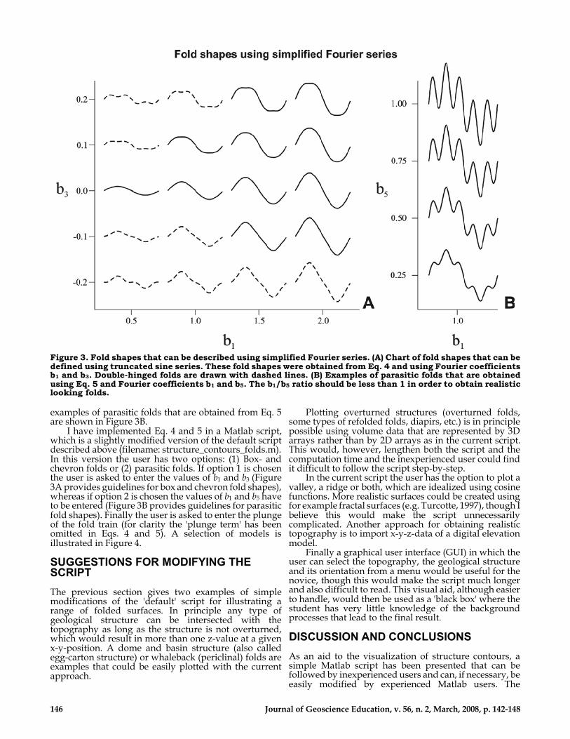
examples of parasitic folds that are obtained from Eq. 5are shown in Figure 3B.

I have implemented Eq. 4 and 5 in a Matlab script,which is a slightly modified version of the default scriptdescribed above (filename: structure_contours_folds.m). In this version the user has two options: (1) Box- andchevron folds or (2) parasitic folds. If option 1 is chosenthe user is asked to enter the values of b1 and b3 (Figure3A provides guidelines for box and chevron fold shapes), whereas if option 2 is chosen the values of b1 and b5 haveto be entered (Figure 3B provides guidelines for parasiticfold shapes). Finally the user is asked to enter the plungeof the fold train (for clarity the 'plunge term' has beenomitted in Eqs. 4 and 5). A selection of models isillustrated in Figure 4.

SUGGESTIONS FOR MODIFYING THESCRIPTThe previous section gives two examples of simplemodifications of the 'default' script for illustrating arange of folded surfaces. In principle any type ofgeological structure can be intersected with thetopography as long as the structure is not overturned,which would result in more than one z-value at a givenx-y-position. A dome and basin structure (also calledegg-carton structure) or whaleback (periclinal) folds areexamples that could be easily plotted with the currentapproach.

Plotting overturned structures (overturned folds,some types of refolded folds, diapirs, etc.) is in principlepossible using volume data that are represented by 3Darrays rather than by 2D arrays as in the current script.This would, however, lengthen both the script and thecomputation time and the inexperienced user could findit difficult to follow the script step-by-step.

In the current script the user has the option to plot avalley, a ridge or both, which are idealized using cosinefunctions. More realistic surfaces could be created usingfor example fractal surfaces (e.g. Turcotte, 1997), though I believe this would make the script unnecessarilycomplicated. Another approach for obtaining realistictopography is to import x-y-z-data of a digital elevationmodel.

Finally a graphical user interface (GUI) in which theuser can select the topography, the geological structureand its orientation from a menu would be useful for thenovice, though this would make the script much longerand also difficult to read. This visual aid, although easierto handle, would then be used as a 'black box' where thestudent has very little knowledge of the backgroundprocesses that lead to the final result.

DISCUSSION AND CONCLUSIONSAs an aid to the visualization of structure contours, asimple Matlab script has been presented that can befollowed by inexperienced users and can, if necessary, be easily modified by experienced Matlab users. The

146 Journal of Geoscience Education, v. 56, n. 2, March, 2008, p. 142-148

Figure 3. Fold shapes that can be described using simplified Fourier series. (A) Chart of fold shapes that can be defined using truncated sine series. These fold shapes were obtained from Eq. 4 and using Fourier coefficients b1 and b3. Double-hinged folds are drawn with dashed lines. (B) Examples of parasitic folds that are obtainedusing Eq. 5 and Fourier coefficients b1 and b5. The b1/b5 ratio should be less than 1 in order to obtain realisticlooking folds.

disadvantage of the script is that complex geologicalstructures that have at a given lateral x-y-position morethan one elevation (z-value) cannot be displayed.Although the implementation would be relativelysimple using volume data, it would lengthen the codeand its simplicity would suffer. The fact that steeplydipping/plunging planes/folds cannot be displayedadequately could also be solved by using volume data,rather than 2D arrays.

The advantage of the script is its simplicity.Consequently novices can follow it step-by-step. As longas the structures are not steep or overhanging a widerange of geological surfaces can be displayed. I believethat the potential educational benefit is two-fold:

1. Students are introduced to Matlab andprogramming in general, which is an increasinglyimportant skill (Middleton, 1999). Since theequations I have used are simple trigonometricfunctions, students should be able to follow howthese equations are implemented in a programminglanguage. Although the script could be used in ablack-box manner without knowledge of theunderlying programming I suggest that thelecturer/student should try to understand each stepin the script. This step-by-step process could clarifythe concept of structure contours and outcroppatterns. Additionally the simple modifications ofthe script presented above (box and chevron folds,parasitic folding) introduce (or revisit, depending on the student's level) the concept of simplified Fourierseries.

2. The 3D Matlab diagrams can be used for illustratingstructure contours and outcrop patterns. Thesediagrams, when plotted in Matlab, can be rotated in3D using the mouse. The student can thereforeinspect the structure from an infinite number ofperspectives (side, top or oblique views) in order totrain his/her spatial visualization abilities and mostimportantly their ability to bisect two objects(topography and geology) in 3D.

I have not conducted thorough quantitative research onthe extend to which usage of the script and its outputenhances the ability of students to visualize in 3D,though feedback from geology and civil engineeringstudents is generally positive. In these classes ourprimary goal was to help student's understanding ofgeology and visualization of geological structures.Understanding the script is certainly a bonus for theenthusiast, but needs to be a secondary goal.

In this paper I have only presented a script thatfocuses on structure contours and outcrop patterns.Matlab is a powerful and easy-to-use software packagethat could, in principle, be used for visualizing a vastrange of geometrical concepts for undergraduatemapping courses, such as the three-point problem, faultsand unconformities. Future studies could broaden thescope of map-related concepts explained using Matlab.

ACKNOWLEDGMENTSFeedback of UCD geology undergraduates,postgraduates and staff is appreciated. John Walsh isacknowledged for useful comments on an earlier versionof this paper. Reviews by Robert Burger and ananonymous reviewer and the editorial advice aregratefully acknowledged.

Schöpfer - Visualizing Structure Contours and Outcrop Patterns 147

Figure 4. Matlab models generated using a modifiedscript. (A) Chevron folds with a wavelength of 500 m,an amplitude of 100 m and Fourier coefficients b1 and b3 of 1.5 and -0.1, respectively. (B) Box folds with awavelength of 500 m, an amplitude of 100 m andFourier coefficients b1 and b3 of 1.5 and 0.2,respectively. (C) Folded surface exhibiting parasiticfolds with a wavelength of 500 m, amplitude of 100 mand Fourier coefficients b1 and b5 of 1.0 and 0.5,respectively.

REFERENCESBennison, G. and Moseley, K., 2003, An Introduction to

Geological Structures and Maps (7th edition),London, Hodder Arnold, 160 p.

Duesbury, R.T., and O'Neil Jr., H.F., 1996, Effect of typeof practice in a computer-aided design environmentin visualizing three-dimensional objects fromtwo-dimensional orthographic projections, Journalof Applied Psychology, v. 81, p. 249-260.

Hudleston, P.J., 1973, Fold morphology and somegeometrical implications of theories of folddevelopment, Tectonophysics, v. 16, p. 1-46.

Kali, Y. and Orion, N., 1996, Spatial abilities ofhigh-school students in the perception of geologicstructures, Journal of Research in Science Teaching,v. 33, p. 369-391.

Libarkin, J.C., and Brick, C., 2002, Researchmethodologies in science education: Visualizationand the geosciences, Journal of GeoscienceEducation, v. 50, p. 449-455.

Lisle, R.J., 2003, Geological Structures and Maps: APractical Guide, Oxford, Butterworth Heinemann,120 p.

Maltman, A., 1998, Geological Maps: An Introduction,New York, John Wiley and Sons Ltd, p. 272.

Matlab, 2002, The MathWorks Inc., Natick,Massachusetts.

Middleton, G.V., 1999, Why geologists should useMatlab, Journal of Geoscience Education, v. 47, p176.

Ramsay, J.G., and Huber, M.I., 1987, The Techniques ofModern Structural Geology, v. 2, Folds andfractures, London, Academic Press Ltd, 391 p.

Spencer, E.W., 1999, Geologic Maps: A Practical Guide tothe Interpretations and Preparation of GeologicMaps, New York, Prentice Hall, 184 p.

Stabler, C.L., 1968, Simplified Fourier analysis of foldshapes, Tectonophysics, v. 6, p. 343-350.

Turcotte, D.L. 1997, Fractals and Chaos in Geology andGeophysics, Cambridge, Cambridge UniversityPress, 412 p.

Twiss, R.J. 1988, Description and classification of folds insingle surfaces, Journal of Structural Geology, v. 10,607-623.

Weijermars, R., 1997, Structural Geology and MapInterpretation, Amsterdam, Alboran Science, 378 p.

148 Journal of Geoscience Education, v. 56, n. 2, March, 2008, p. 142-148