A Matlab Implementation to Assist Model Structure …A Matlab Implementation to Assist Model Structure Analysis (MSA) ROGELIO OLIVA Harvard Business School Morgan Hall T87 Boston,

A Matlab Implementation to AssistModel Structure Analysis (MSA)

ROGELIO OLIVAHarvard Business School

Morgan Hall T87Boston, MA 02163

Ph 617-495-5049 Fx 671-496-5265Email: [email protected]

D-4864-2

D-4864-2 Model Structure Analysis

© R. Oliva, 2003 1

Introduction

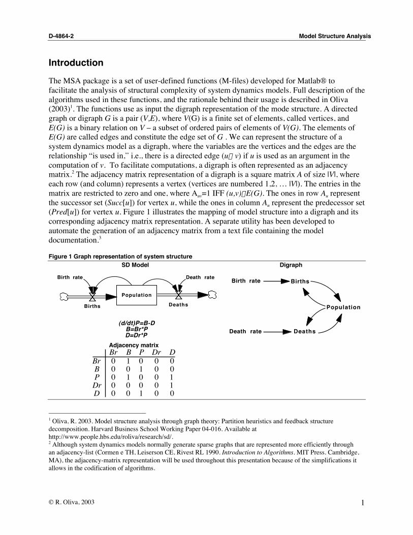
The MSA package is a set of user-defined functions (M-files) developed for Matlab® tofacilitate the analysis of structural complexity of system dynamics models. Full description of thealgorithms used in these functions, and the rationale behind their usage is described in Oliva(2003)1. The functions use as input the digraph representation of the mode structure. A directedgraph or digraph G is a pair (V,E), where V(G) is a finite set of elements, called vertices, andE(G) is a binary relation on V – a subset of ordered pairs of elements of V(G). The elements ofE(G) are called edges and constitute the edge set of G . We can represent the structure of asystem dynamics model as a digraph, where the variables are the vertices and the edges are therelationship “is used in,” i.e., there is a directed edge (uÆv) if u is used as an argument in thecomputation of v. To facilitate computations, a digraph is often represented as an adjacencymatrix.2 The adjacency matrix representation of a digraph is a square matrix A of size |V|, whereeach row (and column) represents a vertex (vertices are numbered 1,2, … |V|). The entries in thematrix are restricted to zero and one, where Auv=1 IFF (u,v)ŒE(G). The ones in row Au representthe successor set (Succ[u]) for vertex u, while the ones in column Au represent the predecessor set(Pred[u]) for vertex u. Figure 1 illustrates the mapping of model structure into a digraph and itscorresponding adjacency matrix representation. A separate utility has been developed toautomate the generation of an adjacency matrix from a text file containing the modeldocumentation.3

Figure 1 Graph representation of system structureSD Model Digraph

Population

Births Deaths

Birth rate Death rate

(d/dt)P=B-DB=Br*PD=Dr*P

Population

Births

Deaths

Birth rate

Death rate

Adjacency matrixBr B P Dr D

Br 0 1 0 0 0B 0 0 1 0 0P 0 1 0 0 1Dr 0 0 0 0 1D 0 0 1 0 0

1 Oliva, R. 2003. Model structure analysis through graph theory: Partition heuristics and feedback structuredecomposition. Harvard Business School Working Paper 04-016. Available athttp://www.people.hbs.edu/roliva/research/sd/.2 Although system dynamics models normally generate sparse graphs that are represented more efficiently throughan adjacency-list (Cormen e TH, Leiserson CE, Rivest RL 1990. Introduction to Algorithms. MIT Press. Cambridge,MA), the adjacency-matrix representation will be used throughout this presentation because of the simplifications itallows in the codification of algorithms.


© R. Oliva, 2003 2

The functions in the MSA package perform a model partition based on data availability, identifythe basic elements of a model structure as defined by Warfield4 –levels, cycles and feedbackloops– and identify and hierarchize a model’s independent loop set5. The package also includesmultiple display and plotting functions to facilitate the analysis and visualization of the system’sstructure. The sequence suggested below illustrates how to use these functions in the context ofmaximizing the use of data available for calibrating the model.

Functions have been tested with Matlab®6 versions 5.2 and 6.5 for Macintosh, and versions 5.2and 5.3 for PC and Unix.7 At one time the functions were implemented for RLab8 –a freewarescientific programming environment similar to Matlab® – but I found it much easier to developthe tools for the IO interface of Matlab®. If someone is interested in implementing the MSApackage for RLab or compiling the package as a stand-alone application please contact me [email protected] or 617-495-5049.

The rest of this document assumes that the user has some familiarity with the use of Matlab®.

Installing MSA functions

After downloading and decompressing the functions,9 you should have a folder entitled MSAwith a series of text documents with the suffix .m10. Move the folder to the Matlab directory andstart up Matlab. Modify Matlab’s current search path to include the MSA folder just installed.

»path(path,'/applications/Matlab/MSA')11

Verify that Matlab has access to the MSA functions with the what command. The commandshould report the 14 M-files contained in the MSA package:

»what MSAdat_partd_cylesd_levelsd_loops

d_predd_succhandlesloop_h

paramp_loopp_predp_succ

reachstructure

3 Oliva, R. 2003. Vensim® Model to Adjacency Matrix Utility. Harvard Business School. Boston, MA. June 02,2003. Available at http://www.people.hbs.edu/roliva/research/sd/.4 Warfield, J.N. 1989. Societal Systems: Planning, policy and complexity. Intersystems Publications. Salinas, CA.5 Kampmann, C.E. 1996. Feedback loop gains and system behavior. Proceedings of the 1996 Int. System DynamicsConference. Cambridge, MA. Pg. 260-263.6 http://www.mathworks.com7 Most of the functions were developed under v4.2. Reinstating v4.2 functionality would only require the unpackingof the subordinated functions included in some M-files.8 http://www.eskimo.com/~ians/rlab.html9 Functions are available at http://www.people.hbs.edu/roliva/research/sd/10 If you have difficulties downloading the .hqx or the .zip archives, you can download one-by-one the 14 functionsusing the text format. Save the functions in a directory entitled MSA and follow the rest of the steps for installation.11 The syntax of the path command varies from platform to platform to match the directory description syntax ofthe operating system. Check help path on the Matlab prompt for more details.


© R. Oliva, 2003 3

A basic description of each function’s usage as well as the specification of the required inputsand generated outputs can be obtained through the help command at the Matlab prompt:

»help function_name

Suggested sequence for Model Structure Analysis

The functions in the MSA package are quite versatile and can be used in different ways todevelop an intuition about the structural complexity of a model. The following steps have provento be a successful sequence to develop such intuition, but in no way are they intended to be theonly way to use the MSA functions. The sequence makes use and illustrates the functionality ofthe 14 functions included in the MSA package. For more information on each function use thehelp command at the Matlab prompt.

1. Load model structure and names

Assign the adjacency matrix describing the system structure and the variable name matrix tovariables in the current workspace. MATLAB *.m file generated by the Vensim® Model toAdjacency Matrix Utility contains a simple function, named as the original model, that returnsthe adjacency matrix and the name list for model variables into a structured array withcomponents .adj and .nms. See the READ_ME file12 for the Vensim® Model to AdjacencyMatrix Utility for instructions on how to generate the *.m files to import them into MATLAB(Make sure that the *.m files containing the structure and the names are in a path whereMATLAB can find them).

»A=my_model;

Each component of the structured array can be reached through sub-indexing. The adjacencymatrix (a sparse squared binary matrix with the same number of rows as model variables) isaccessible in A.adj, and the list of names (character vector) in A.nms.

The spy command can give you a sense of the density of interconnections in the model structure;a point in the sparcity graph represents a direct interconnection between variables.

»spy(A.adj)

A traditional equation-by-equation report of the system structure can be generated using the'display' commands for predecessors and successors. d_pred lists all the variables that go into anequation –equivalent to the relationship uses– and d_succ lists all the equations where a variableis utilized –equivalent to the relationship used in.

»d_pred(A,VARS)»d_succ(A,VARS)

12 http://www.people.hbs.edu/roliva/research/sd/mdl2bin_READ_ME.htm


© R. Oliva, 2003 4

If variable numbers (VARS) are not specified, these functions will list the predecessors andsuccessors for ALL model variables.

It is also possible to identify the model parameters –elements without predecessors– from theadjacency matrix and identify the elements where parameters are being used:

»PRM=param(A);»d_succ(A,PRM);

To list of parameters, or access the name of any model variable, it is possible to call directly intothe .nms partition of the adjacency matrix.

»A.nms(PRM,:)»A.nms(17,:)»A.nms([13 16 20],:)

2. Identify data availability

Incorporate in a vector the variables for which time series are available:

»DATA=[2 8 26 33 45 49]

At this stage is possible to visualize the potential impact of data availability on determining othermodel variables.

»p_succ(A,DATA);

3. Partition model according to data availability.

The dat_part function partitions a system described as an adjacency binary matrix (ADJ)according to data availability (DATA).

»PART=dat_part(A,NMS)

The output, PART, is a structure that for each data series available contains the sub-components[y,x,beta,eqs] corresponding to the dependent variable, independent variables, parametersthat can be estimated and equations involved in the estimation. Each component of the structurecan be reached through the following sub-indexing:

PART.y, PART.x, PART.beta and PART.eqs.

The full specification of equation i can be reached by just specifying the subindex in the PARTstructure:

»PART(i)

An individual component can be reached by specifying the subindex in the PART structure (theequation number) AND the component:


© R. Oliva, 2003 5

»PART(1).y»PART(1).x»PART(3).beta»PART(2).eqs

In the unlikely case that all parameters are reachable with the existing data, steps 1 through 4 isall that might be needed in terms of structural analysis. Most of the time, however, it will benecessary to develop a strategy on how to do the partial model calibrations so that data andinsights from other sections of the model can be used in the process.

4. Generate the reachability matrix for the model.

Although it is not needed for the analysis of the system structure (all the information in it iscontained in the ADJ matrix), it gives a clear visual indication of how densely connected themodel really is. While SD models normally generate sparse adjacency matrices (variables areaffected only by two or three other variables), the reachability matrices of SD models tend tohave very high densities due to the number of feedback loops in the structure. The reachfunction returns an array with the same structure as the adjacency matrix – with subcomponents.adj (sparse square binary matrix) and .nms (character array with variable names).

»R=reach(A);»spy(R.adj);

5. Identify elements of model structure: levels, cycles and feedback loops

Run basic function to decompose the structure of the system into levels, identify the ShortestIndependent Loop Set (ILS) or the Minimal Shortest Independent Loops Set (MSILS) for themodel,13 and order the model variables in a way to minimize the distance of interactions to themain diagonal of the adjacency matrix.

»STR=structure(A); % For SILS»STR=structure(A,-1); % For MSILS

The function returns an arrayed structure with five components:

adj (sparse-binary) a replica of the input matrix.

nms (character vector) a replica of the input name vector.

lev (sparse-binary) each row identifies the elements that belong to a level partition.

cyc (sparse-binary) each row identifies the elements that belong to a cycle.

ecc (sparse) each row contains the eccentricity of the elements of a cycle.

13 See Oliva, R. 2003. Model structure analysis through graph theory: Partition heuristics and feedback structuredecomposition. Harvard Business School Working Paper 04-016. Available athttp://www.people.hbs.edu/roliva/research/sd/.


© R. Oliva, 2003 6

fbl (array of double) for every cycle partition, a matrix contains in each row the orderedset of elements the feedback loops that constitute the shortestindependent loop set.

idx (structure) diverse information to facilitate the plotting of the sparsity pattern.

Each component can be reached wit a three-letter subindex in lower case: STR.adj, STR.nms,STR.lev, STR.cyc, STR.ecc, STR.fbl, and STR.idx.

The function identifies separately the elements in a cycle (cyc). The mapping of each cycle intoits corresponding level is reported in the progress output that the function generates, and allelements of the cycle partition are included in their corresponding level (lev).

ecc is a matrix that has a row for each cycle partition. Each cell contains the eccentricity of theelements belonging to that cycle partition with respect to the cycle partition –the entry for a nodenot belonging to the cycle partition is 0. Eccentricity of a node is defined (in graph theory) as thelongest of the shortest paths between that node and every other node in the graph –this measureshow far the node is of its furthest node in the cycle partition. The nodes with the smallestexcentricity are said to be in the center of the graph.

fbl is an array that contains a matrix for each cycle partition. In these matrices, each row has theordered set of elements in a feedback loop. Self reference loops are not reported (loops of length1), and the loop list is sorted by loop length (from shortest to longest). Note that fbl contains theSILS or MSILS (depending on selected option) for each cycle partition –each reported loop islinearly independent, and, in the case of the MSILS, there are no redundant loops in the reportedset.14

idx contains a structure with three different components to facilitate displaying the sparsitypattern of the adjacency matrix. The first part (idx) contains and index of all the nodes orderedby level, including the cycle elements within the level, and orders elements within a level tominimize the distance of interactions to the main diagonal –bandwidth. The other two elementsof idx (tks and lbl) contain information about the level partition to be used by the p_pred andp_succ functions.

5a. Displaying the model structure

At this stage is possible to see the elements of the model structure with the following 'display'functions:

»d_levels(STR,PRT)»d_cycles(STR,PRT)

Each function generates the list of elements that belong to partition PRT. If no partition number(PRT) is specified when calling these functions, the elements of ALL partitions are listed. The

14 See Oliva (2003) for formal definition of Shortest Independent Loop Set and Minimal Shortest Independent LoopSet.


© R. Oliva, 2003 7

d_cycles function also reports node eccentricity within the cycle and sorts the output by nodeeccentricity (from the center of the graph to its edges).

The function

»d_loops(STR,PRT,LPN);

displays the variable names of the elements of the LPN feedback loop in the PRT cycle partition.If no loop number (LPN) is provided, the function lists the elements of all the loops in theidentified cycle partition. If no cycle partition (PRT) is provided, the function lists the elementsof ALL the feedback loops in the model.

Depending on the type of analysis you are doing, you might find it useful to create vectors withthe elements of each level, cycle, or feedback loop. The function handles creates a set ofhandles to the set of partitions included in the structured matrix STR.

»H=handles(STR)

Handles are provided for levels (H.l01, H.l02 ...) cycles (H.c01, H.c02 ...) andfeedback loops. The handles for feedback loops are provided with 3 digits PLL (H.f101,H.f102 ... H.f201, H.f202 ...) where P is a cycle partition and LL the

The display functions d_pred and d_succ –defined above– also function taking in the fullstructured array matrix or handles as input.

»d_pred(STR,VARS);»d_succ(STR,VARS);»d_pred(STR,H.f###);»d_succ(STR,H.l###);

Two ‘plotting’ functions, p_pred and p_succ, further facilitate the exploration of the sparcitypattern of the adjacency and reachability matrices highlighting in a different color thepredecessors or successors of a selected group of variables. The following are suggested uses forthese functions to visualize the segmentation of the model structure.

»p_pred(A,H.l01);»p_pred(STR,3);»p_pred(R,H.l##);»p_succ(R,[4 5 16]);»p_pred(R,PRM);»p_succ(STR,PRM);

If the input matrix for the plotting functions is the full structural array STR (the output of thestructure function), the sparsity plot is sorted by level partitions and the partitions are identifiedin the plot.

Loops can be traced in the sparcity graph using the function p_loop (note that it only takes asinput the full structural array STR):


© R. Oliva, 2003 8

»p_loop(STR,LOOP#)»p_loop(STR,LOOP#,0) for the sparcity graph not to be sorted by STR.idx.idx.

LOOP# can either be a loop handle (see handle function), or a direct reference to a loop accordingto the PLL format, where P is a digit referring to the cycle partition, and LL are two digitsidentifying the loop within the partition.

The sorted matrix and visual analysis of the sparcity graphs created with p_pred and p_succallow the development of a sequence of estimation steps –from high to low level variables– thatcreate new data as confidence is developed in partial sections of the model.

As more parameters are estimated and the estimation process yields reliable values forintermediate variables, these new data series can be incorporated into the data set (step 3) and themodel can be re-partitioned with the new data availability.

Unfortunately, most of the complexity in SD models lies in the feedback loops –normallycontained in one or two cycle sets– and a times is necessary to explore the relationships amongfeedback loops to maximize the value of the data available.

6. Identify loop hierarchy

The function loop_h develops a loop hierarchy of the loops in a particular cycle partition (PRT),based on the inclusion relation. A loop A is said to be included in loop B one if all the elementsof A are also present in B.

»LPS=loop_h(STR, PRT)

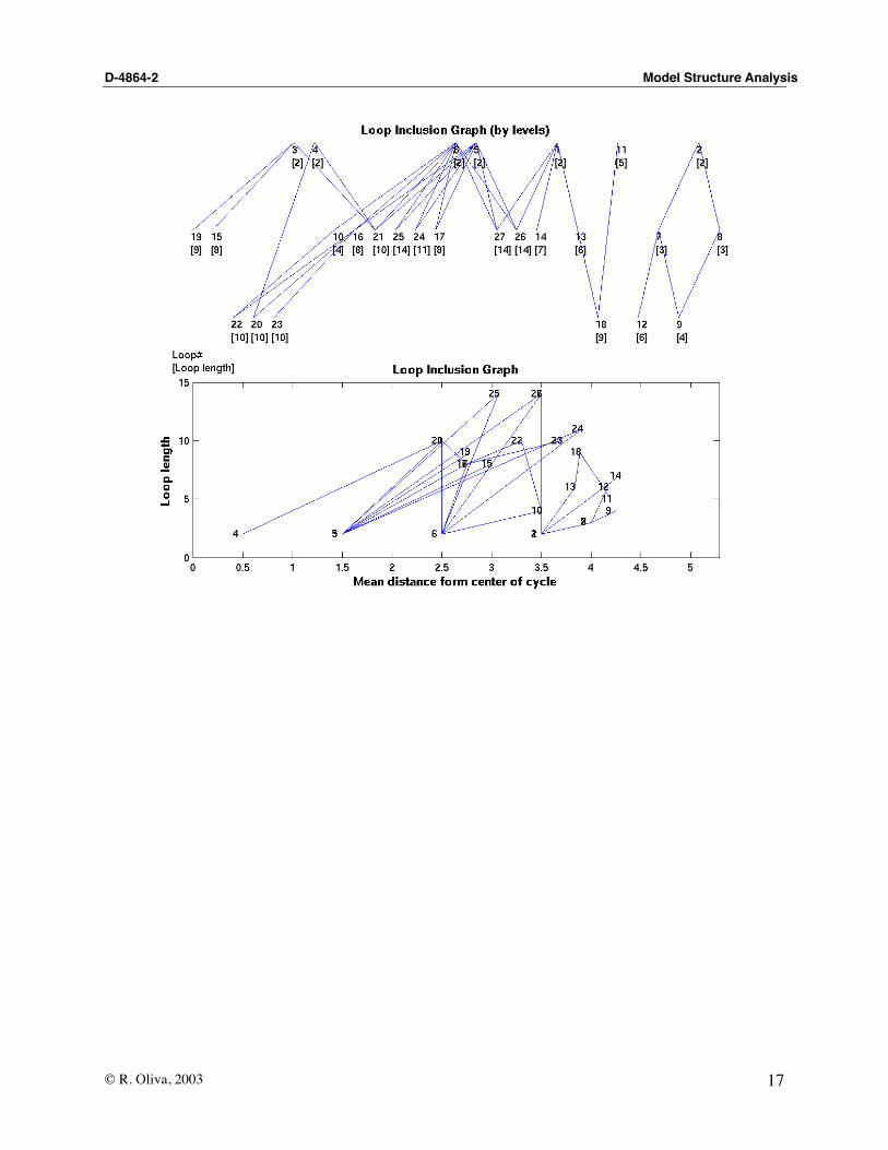
The result is presented as a level structure matrix LPS.lev and the corresponding matrix ofinclusions LPS.str. The function also generates two plots of the inclusion graph. BecauseSTR.fbl is an independent loop set (a great simplification from the total number of feedbackloops normally available in a SD model), the loop hierarchy structure does not contain cyclepartitions, is relatively flat (2 to 4 levels), and not many 'inclusions' (loops contained in otherloops) are found. The inclusion graph, however, can be used to develop an incremental testingsequence vase on building confidence in simple structures first –the inner loops in the model–and moving into more complex and interdependent structures. The first plot o

(Note that neither the length of the loop nor its relative position in the loop hierarchy structure,has anything to do with its relative dominance of the system’s behavior).


© R. Oliva, 2003 9

Appendix A.

Direct access to model structure.

It is possible to access the partitions in the STR matrix directly using regular MATLABcommands. The elements of a row i in the lev or cyc matrices can be identified through thefollowing commands:

»find(STR.lev(i,:))»STR.nms(find(STR.lev(i,:)),:) to see the variable names.»find(STR.cyc(i,:))»STR.nms (find(STR.cyc(i,:)),:) to see the variable names.

The elements of the i loop in the j cycle partition can be reached through the followingcommand:

»nonzeros(STR.fbl(i,:,j))»STR.nms(nonzeros(STR.fbl(i,:,j)),:) to see the variable names.

The index is useful to visualize the clustering of relationships and the "tightly-coupled sectors ofthe model".

»spy((A(STR.ixd.idx,STR.idx.idx));»spy((R(STR.ixd.idx,STR.idx.idx));

To see the name of a specific variable i in the indexed sparsity plot:

»STR.nms(STR.idx.idx(i,:))


© R. Oliva, 2003 10

Appendix B.

Example

The following sequence of commands illustrates the use of the functions and the output theygenerate for a sector of the model used by Oliva and Sterman on their study of erosion of servicequality15. The MODEL.m file containing the adjacency matrix (.adj) and a name list (.nms)was created using the Vensim® Model to Adjacency Matrix Utility.

The following conventions will be followed for the reminder of the appendix:a) Commands given to MATLAB will be in bold; “%” indicates the beginning of a

commentb) Function output in regular text; “…” indicates that part of the output has been omitted

First, this information is loaded into the MATALAB workspace’s variables A.

»A=model % load adjacency matrixA = nms: [78x40 char ] adj: [78x78 sparse]

»spy(A.adj) % see sparsity pattern for A

15 Oliva, R., and J. D. Sterman. "Cutting Corners and Working Overtime: Quality Erosion in the Service Industry."Management Science 47, no. 7 (July 2001): 894-914. The model is fully documented and available at:http://www.people.hbs.edu/roliva/research/service/esq.html. The model used for this example is the same modelavailable in the website but without the variables in the quality sector that were not active in the final calibration ofthe model.


© R. Oliva, 2003 11

»d_pred(A,9) % id predecesors for variable 9work pressure service capacity desired service capacity

»d_succ(A,9) % id successors for variable 9work pressure work intensity effect of wp on to

»P=param(A) % id model parametersP = Columns 1 through 12 3 8 12 14 15 17 19 20 22 23 25 27 Columns 13 through 24 30 31 33 34 36 40 41 43 45 47 48 50 Columns 25 through 35 52 56 61 62 63 72 73 75 76 77 78

»A.nms(P,:) % list names of model parametersMIN RESIDENCE T FOR AN ORDER DESIRED DELIVERY DELAY BETA ...a absenteeism HWE

»d_succ(A,P) % see immediate succesors of model parametersMIN RESIDENCE T FOR AN ORDER order fulfillment DESIRED DELIVERY DELAY desired service capacity BETA work intensity ...a absenteeism absenteeism HWE on office service capacity Perceived Labor Productivity Desired Labor absenteeism

»D=[1 2 5 10 11 35 37 38 49 70 74] %id vars. for which data is availableD = 1 2 5 10 11 35 37 38 49 70 74

»A.nms(D,:) % list variables for which data is availableans =Service Backlog order fulfillment service capacity time per order


© R. Oliva, 2003 12

work intensity Desired Labor turnover rate total labor hiring rate customer orders absenteeism

»dat_part(A,D) % execute the data availability partitionIdentifying model parameters ......y: time per order x: service capacity Service Backlog beta: MIN PROCESSING TPO ALPHA DESIRED DELIVERY DELAY TTDN TTUP eqs: time per order effect of wp on to Desired To work pressure dto chg desired service capacity t to adjust dto ...Parameters not reachable from data available: INITIAL FE INITIAL FA INITIAL DTO INITIAL P ELF INITIAL EXPERIENCED PERSONNEL INITIAL ROOKIES INITIAL VACANCIES TPO ON DQ GRAPH QP ON TO GRAPH ans =1x11 struct array with fields: y x beta eqs

»R=reach(A) % generate the reachability matrixR = adj: [78x78 sparse] nms: [78x40 char ]


© R. Oliva, 2003 13

»spy(R.adj) % see sparsity pattern for R

»S=structure(A) % identify elements of model structureCalculating Reachability Matrix ...Identifying Level Partitions ... Cycle 1 belongs to level 2. Identifying Loops within Cycle 1 ... Reducing Cycle 1 to Independent Loop Set ...Indexing Variables by Level ...S = adj: [78x78 sparse] nms: [78x40 char ] lev: [ 5x78 sparse] cyc: [ 1x78 sparse] ecc: [ 1x60 sparse] fbl: [23x14 double] idx: [ 1x1 struct]

»d_cycles(S,1) % list elements of 1st (only) cycle partitionCycle 1 Ecc Variable 7 Rookies 8 turnover rate 8 total labor ... 14 Desired Labor 15 Perceived Labor Productivity

»d_levels(S,3) % list elements of 3rd level partition –vars &parameters that feed into the cycle partition

Level 3 MIN RESIDENCE T FOR AN ORDER DESIRED DELIVERY DELAY BETA


© R. Oliva, 2003 14

... customer orders absenteeism

»d_loops(S) % list loops in model (all in first cycle)Cycle 1 Loop 1 Service Backlog order fulfillment Loop 2 Desired To dto chg Loop 3 Rookies experience rate ... Loop 23 Service Backlog desired service capacity Desired Labor replacement rate desired hiring indicated labor order rate labor order rate Vacancies hiring rate Rookies effective labor fraction service capacity potential order fulfillment order fulfillment

»d_loops(S,1,16) % list elements of loop 16 (first cycle partition) Loop 16 Service Backlog desired service capacity work pressure work intensity Fatigue E effect of fatigue on prod service capacity potential order fulfillment order fulfillment

»H=handles(S) % create hanldels for model partitionsH = l01: [14 19 27 33 43 45 52 62 63 64 65 66 67 68 69]... l05: 72 c01: [1x34 double] f101: [1 2]... f123: [1 7 35 58 57 54 60 51 49 44 39 5 4 2]


© R. Oliva, 2003 15

»p_pred(S,H.l01) % show predecesors to variables in level 01

»d_pred(S,H.l01) % list predecesors to variables in level 01INITIAL FE INITIAL FA INITIAL P ELF ...average productivity of labor service capacity total labor

»p_succ(S,P) % show succesors to model parameters


© R. Oliva, 2003 16

»p_succ(A,P) % same information in original adj. matrix

»p_loop(S,123) % show indicence of loop 23 on partition 1

»L=loop_h(S,1); % show loop hierarchy structure (cycle 1)Identifying inclusions within cycle loop set ...Reducing to Adjacency Matrix ...Calculating Reachability Matrix ...Identifying Level Partitions ...Indexing for plot coordenates ...L = lev: [ 3x23 sparse] str: [23x23 sparse]


© R. Oliva, 2003 17

Documents

A Matlab Implementation to Assist Model Structure …A Matlab Implementation to Assist Model Structure Analysis (MSA) ROGELIO OLIVA Harvard Business School Morgan Hall T87 Boston,