Embed Size (px)
Citation preview

A mathematician is a device for turning coffee into theorems.
– Alfred Renyi
Math is hard.
– Barbie
University of Alberta
MINIMUM DEGREE SPANNING TREES ON BIPARTITEPERMUTATION GRAPHS
by
Jacqueline Smith
A thesis submitted to the Faculty of Graduate Studies and Researchin partial fulfillment of the requirements for the degree of
Master of Science
Department of Computing Science
c©Jacqueline SmithSpring 2011
Edmonton, Alberta
Permission is hereby granted to the University of Alberta Libraries to reproduce singlecopies of this thesis and to lend or sell such copies for private, scholarly or scientific
research purposes only. Where the thesis is converted to, or otherwise made available indigital form, the University of Alberta will advise potential users of the thesis of these
terms.
The author reserves all other publication and other rights in association with the copyrightin the thesis, and except as herein before provided, neither the thesis nor any substantialportion thereof may be printed or otherwise reproduced in any material form whatever
without the author’s prior written permission.

To my parents, Jim and Jennifer.
Abstract
The minimum degree spanning tree problem is a widely studied NP-hard variation
of the minimum spanning tree problem, and a generalization of the Hamiltonian
path problem. Most of the work done on the minimum degree spanning tree prob-
lem has been on approximation algorithms, and very little work has been done
studying graph classes where this problem may be polynomial time solvable. The
Hamiltonian path problem has been widely studied on graph classes, and we use
classes with polynomial time results for the Hamiltonian path problem as a starting
point for graph class results for the minimum degree spanning tree problem. We
show the minimum degree spanning tree problem is polynomial time solvable for
chain graphs. We then show this problem is polynomial time solvable on bipartite
permutation graphs, and that there exist minimum degree spanning trees of these
graphs that are caterpillars, and that have other particular structural properties.

Acknowledgements
First, I would like to express my gratitude to my supervisor, Lorna Stewart, for
her support and encouragement. Her guidance led to my successful completion of
this thesis, and to my development as a researcher. I would also like to thank my
committee members, Joe Culberson and Gerald Cliff, for their useful feedback on
this work.
Thanks to Marc Bellemare for being my sounding board, for being able to do
algebra, and for keeping me motivated through the hard parts. Many thanks also go
to Rick Valenzano for preserving my sanity, and helping me keep things in perspec-
tive.
Finally, I am forever grateful to my friends and family for their love and support,
and for tolerating me trying to teach them about graphs.
Table of Contents
1 Introduction 11.1 Overview . . . . . . . . . . . . . . . . . . . . . . . . . . . . . . . 11.2 Motivation . . . . . . . . . . . . . . . . . . . . . . . . . . . . . . . 21.3 Definitions and Graph Classes . . . . . . . . . . . . . . . . . . . . 31.4 Problem Definitions . . . . . . . . . . . . . . . . . . . . . . . . . . 81.5 Contributions . . . . . . . . . . . . . . . . . . . . . . . . . . . . . 10
2 Background 112.1 Complexity, Related Problems, and Variations on the Minimum De-
gree Spanning Tree Problem . . . . . . . . . . . . . . . . . . . . . 112.2 Approximations . . . . . . . . . . . . . . . . . . . . . . . . . . . . 15
2.2.1 Unweighted Approximations . . . . . . . . . . . . . . . . . 152.2.2 Weighted Approximations . . . . . . . . . . . . . . . . . . 16
2.3 Hamiltonicity and k-trees . . . . . . . . . . . . . . . . . . . . . . . 182.4 Vertex Orderings and Properties of Bipartite Graph Classes . . . . . 222.5 Algorithms and Complexity for Hamiltonicity and other Related
Problems on Graph Classes . . . . . . . . . . . . . . . . . . . . . . 242.6 Properties of Trees . . . . . . . . . . . . . . . . . . . . . . . . . . 28
3 Chain Graphs 303.1 A Degree Condition for Hamiltonian Chain Graphs . . . . . . . . . 313.2 A Minimum Degree Spanning Tree Construction Algorithm for
Chain Graphs . . . . . . . . . . . . . . . . . . . . . . . . . . . . . 323.2.1 Algorithm . . . . . . . . . . . . . . . . . . . . . . . . . . . 333.2.2 Proof of Correctness . . . . . . . . . . . . . . . . . . . . . 41
3.3 Solving the Minimum Degree Spanning Tree Problem on ChainGraphs . . . . . . . . . . . . . . . . . . . . . . . . . . . . . . . . . 48
4 Bipartite Permutation Graphs 514.1 Properties of Longest Paths . . . . . . . . . . . . . . . . . . . . . . 524.2 Crossing-Free Minimum Degree Spanning Trees . . . . . . . . . . 634.3 Longest Paths in Minimum Degree Spanning Trees . . . . . . . . . 754.4 An Algorithm for ∆∗G of a Bipartite Permutation Graph . . . . . . . 91
5 Conclusion 965.1 Summary . . . . . . . . . . . . . . . . . . . . . . . . . . . . . . . 965.2 Future Work . . . . . . . . . . . . . . . . . . . . . . . . . . . . . . 97
Bibliography 99

List of Tables
2.1 Complexity results for the Hamiltonian path and longest path prob-lems for certain graph classes . . . . . . . . . . . . . . . . . . . . . 28
List of Figures
1.1 A hierarchy of the graph classes discussed in this thesis. For eachclass, its superclasses are above it and subclasses are below. . . . . . 6
1.2 A tree is a caterpillar if and only if it does not contain this subgraph. 7
2.1 Complexities of finding a spanning tree T with ∆(T ) ≤ ∆T in ak-connected general or planar graph G with ∆(G) bounded. [15] . 20
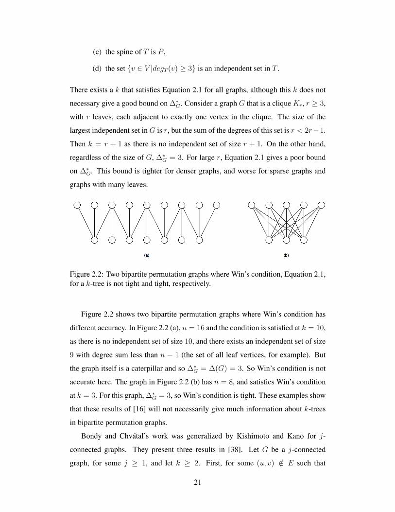
2.2 Two bipartite permutation graphs where Win’s condition, Equation2.1, for a k-tree is not tight and tight, respectively. . . . . . . . . . . 21
2.3 A bipartite graph with X and Y ordered as in a strong ordering of G. 232.4 A graph with a nested neighbourhood ordering. . . . . . . . . . . . 232.5 Two longest paths in a bipartite graph: (a) is not a zig zag, while (b)
is a zig zag. . . . . . . . . . . . . . . . . . . . . . . . . . . . . . . 24
3.1 A chain graph with degrees, ai and bi, labeled. . . . . . . . . . . . 343.2 A chain graph partitioned. From left to right, the parts are C2, C3,
and C1. . . . . . . . . . . . . . . . . . . . . . . . . . . . . . . . . 353.3 Constructing spanning trees on each part. . . . . . . . . . . . . . . 363.4 A spanning tree is constructed on each part in the partition of a
chain graph. . . . . . . . . . . . . . . . . . . . . . . . . . . . . . 363.5 Spanning trees on each part are connected to form a spanning tree
for the graph. . . . . . . . . . . . . . . . . . . . . . . . . . . . . . 373.6 A chain graph. . . . . . . . . . . . . . . . . . . . . . . . . . . . . . 453.7 The chain graph from Figure 3.6, partitioned and with each Ti con-
structed as in PartMDST. . . . . . . . . . . . . . . . . . . . . . . . 453.8 The final edges connecting each Ti from Figure 3.7 to form a span-
ning tree. The vertices xa and yb are labeled in each part, and thebold edge is (xa−1, yb). . . . . . . . . . . . . . . . . . . . . . . . . 46
4.1 A bipartite graph with X and Y ordered as in a strong ordering of G. 524.2 The edges in G if a vertex v /∈ P has some neighbour u /∈ P . . . . 554.3 An MDST with leftmost crossing further right is constructed for
Case 1. . . . . . . . . . . . . . . . . . . . . . . . . . . . . . . . . 654.4 An MDST with leftmost crossing further right is constructed for
Case 2, Subcase A. . . . . . . . . . . . . . . . . . . . . . . . . . . 664.5 An MDST with leftmost crossing further right is constructed for
Case 2, Subcase B. . . . . . . . . . . . . . . . . . . . . . . . . . . 674.6 A nearer crossing is created in Case 2, Subcase D. . . . . . . . . . 694.7 A nearer crossing is created for Case 2, Subcase D. . . . . . . . . . 704.8 Case 3 can be reduced to Case 1 or Case 2, depending on the de-
grees of xi2 and yj2 . . . . . . . . . . . . . . . . . . . . . . . . . . 704.9 A new MDST with leftmost edge crossing further right can be con-
structed in Case 4, Subcase A. . . . . . . . . . . . . . . . . . . . . 71
4.10 A new MDST with leftmost edge crossing further right can be con-structed in Case 4, Subcase B if an edge can be added between Txand Ty. . . . . . . . . . . . . . . . . . . . . . . . . . . . . . . . . 72
4.11 In Case 4, Subcase B, if the degree of yj1 is decreased, we havereduced this case to Case 3. . . . . . . . . . . . . . . . . . . . . . 73
4.12 A new MDST with leftmost edge crossing further right can be con-structed in Case 4, Subcase B if the degree of xi2 can be decreased. 73
4.13 A new MDST with leftmost edge crossing further right can be con-structed in Case 4, Subcase C if an edge can be added between Txand Ty. . . . . . . . . . . . . . . . . . . . . . . . . . . . . . . . . 74
4.14 If the degree of xi2 can be decreased in Case 4, Subcase C, then thiscase can be reduced to Case 4, Subcase B. . . . . . . . . . . . . . . 75
4.15 Edge crossings in TS can be removed by constructing a zig-zagHamiltonian path on the subgraph of G induced by TS . . . . . . . . 76
4.16 An example of a crossing of two leaf edges, removed as in Step 2a,Case 1. . . . . . . . . . . . . . . . . . . . . . . . . . . . . . . . . 78
4.17 In Step 2a, Case 2, if yj2 < yj3 , we can extend the spine. . . . . . . 804.18 A crossing of two leaves both in X is removed in Step 2b. . . . . . 814.19 If yj2 has no leaves, T ′ has fewer crossings of leaf and spine edges. 824.20 If yj2 has a leaf, T ′ has a longer spine than T . . . . . . . . . . . . . 834.21 Two adjacent spine vertices with leaves imply the spine can be ex-
tended. . . . . . . . . . . . . . . . . . . . . . . . . . . . . . . . . 854.22 By Step 5, crossings of one spine edge and one leaf edge can be
eliminated. . . . . . . . . . . . . . . . . . . . . . . . . . . . . . . 86
5.1 The longest path on the left is not contained in any MDST of thegraph. On the right is a spanning tree with maximum degree threeand so ∆∗ ≤ 3. . . . . . . . . . . . . . . . . . . . . . . . . . . . . 97
Chapter 1
Introduction
1.1 Overview
A spanning tree of a graph is a minimum set of edges that connect all the vertices
of the graph. A minimum degree spanning tree is a spanning tree of a graph with
the restriction that the maximum degree of a vertex in the tree is minimized. The
problem of finding the minimum maximum degree of a spanning tree is NP-hard
in general. Thus, it is believed that there is no polynomial time algorithm for the
problem. The best approximation algorithm finds a solution that is within one of
the optimal value.
For a given NP-hard problem, there may exist restricted graph classes with par-
ticular properties that allow a polynomial time solution to be found to solve the
problem on that class. The minimum degree spanning tree problem is a general-
ization of the problem of finding a Hamiltonian path in a graph, which is NP-hard
in general. The Hamiltonian path problem is well-studied on graph classes and the
problem is known to be polynomial time solvable on many classes.
In this thesis, we first motivate and define the minimum degree spanning tree
problem, present some background and related work, and then show that the prob-
lem can be solved in polynomial time on chain graphs and bipartite permutation
graphs. We also give a number of structural results for the longest path problem
and the minimum degree spanning tree problem on bipartite permutation graphs.
1
1.2 Motivation
While there is a good approximation algorithm for this problem, it is still worth-
while to study this problem on graph classes as the complexity of the problem was
previously unknown on most classes. The minimum degree spanning tree problem
on graph classes is interesting from a theoretical standpoint to discover where the
boundary is between classes where the problem is NP-hard and where it is polyno-
mial time solvable. It is also interesting to compare the boundary for this problem
to the boundary for the Hamiltonian path and longest path problems.
There is only a small amount of work done on solving the minimum degree
spanning tree problem on graphs with particular properties. Czumaj and Stroth-
mann [15] studied k-connected and planar graphs and gave some complexity re-
sults on finding a spanning tree in these graphs with maximum degree less than
some bound, when certain degree conditions were satisfied. To the best of our
knowledge, there does not exist any other work on the minimum degree spanning
tree problem for restricted graph classes. Our work begins to fill in that gap.
The Hamiltonian path problem is a restricted version of the minimum degree
spanning tree problem, and the longest path problem is a generalization of the
Hamiltonian path problem that is related to the minimum degree spanning tree prob-
lem. These problems have polynomial time solutions on many graph classes. Both
of these problems are linear time solvable on bipartite permutation graphs.
The class of bipartite permutation graphs is the graph class we focus on most
in this thesis. Bipartite permutation graphs have a strong ordering of their vertices.
This ordering has adjacency and enclosure properties that allow for polynomial
time solutions to problems that are NP-hard in general. In addition to the Hamil-
tonian path problem and the longest path problem, a number of other polynomial
time algorithms for generally hard problems exist for this class. Examples of other
problems solved for bipartite permutation graphs include the path cover problem
and the edge domination problem.
Furer and Raghavachari [25] mention some practical applications of the mini-
mum degree spanning tree problem in areas such as non-critical network broadcast-
2
ing. Reducing the maximum work done by each node in a network in propagating a
message is critical in networks with constraints on resources like power. Addition-
ally, there is a cost associated with splitting a message from one node to several,
and one might want to reduce the number of splits made by a node. The minimum
maximum degree of a spanning tree of a graphG plays an important role in the edge
reconstruction conjecture. Graphs with at least cn log ∆∗G edges, where ∆∗G is the
minimum maximum degree of a spanning tree of G, are edge-reconstructible [8].
Although few polynomial time exact algorithms for graph classes are known,
the minimum degree spanning tree problem and its variations have been widely
studied in other contexts. In Chapter 2, we discuss work done in this area.
1.3 Definitions and Graph Classes
A graph G is a pair of sets (V,E), where V is a set of vertices and E is a set of
unordered pairs (u, v), called edges, such that u, v ∈ V . Let n = |V | and m = |E|.
We may refer to V and E as V (G) and E(G) if the context is not clear. The order
of a graph G is the number of vertices, n. A graph G = (V,E, c) is a weighted
graph, with cost function c from E to R. A graph G = (V, F ) is directed if F is a
set of ordered pairs (u, v), u, v ∈ V , instead of unordered pairs. We will deal only
with undirected graphs in this thesis. An edge is incident on a vertex v if the edge
is (u, v) for some u.
A subgraph of a graph G = (V,E) is a graph G′ = (V ′, E ′) with V ′ ⊆ V and
E ′ ⊆ E. A spanning subgraph of a graph G is a subgraph of G that contains all
vertices ofG. An induced subgraph of a graphG = (V,E) is a graphG′ = (V ′, E ′)
such that V ′ ⊆ V and E ′ = {(u, v)|u, v ∈ V ′ and (u, v) ∈ E}.
The complement of a graph G = (V,E) is the graph G = (V,E) such that
(u, v) ∈ E if and only if (u, v) /∈ E, for all u, v ∈ V .
A path is a sequence of vertices v1, v2, ..., vk with edges (vi, vi+1) for 1 ≤ i < k
and with vi 6= vj for all i 6= j. The size of the path P is k, the number of vertices in
the path, denoted |P |. The length of the path is k − 1, the number of edges in the
path. Vertices v1 and vk are endpoints of the path. A (u, v)-path is a path with u and
3
v as endpoints. A cycle is a sequence of vertices v1, v2, ..., vk with edges (vi, vi+1)
and (vk, v1), for 1 ≤ i < k and with vi 6= vj , for all i 6= j. A walk is a sequence of
vertices v1, v2, ..., vk with edges (vi, vi+1) for 1 ≤ i < k. Vertices may be repeated.
A walk is a closed walk if v1 = vk.
A graph is connected if for every pair of vertices u, v ∈ V there exists a path
in G from u to v. A connected component of a graph is a maximal connected
subgraph of G; c(G) is the number of connected components in G. A clique in a
graph is a set of vertices K such that every pair of vertices in K is connected by an
edge. An independent set is a set of vertices I ⊆ V such that for all pairs u, v ∈ I ,
(u, v) /∈ E. The independence number of a graph G, denoted α(G), is the size of
the largest independent set in G. Let S be a set of vertices such that S ⊆ V . We
define G − S to be the subgraph of G constructed by removing the vertices in S
and all their incident edges. A cutset of a connected graph G = (V,E) is a set of
vertices S ⊂ V such that G− S has more than one connected component. A graph
is k-connected if it remains connected if less than k vertices are deleted from the
graph. Equivalently, a graph is k-connected if its smallest cutset is of size k.
Vertices u and v are adjacent if (u, v) ∈ E. The neighbourhood of v is the set of
all vertices adjacent to v in G, and is denoted NG(v). The degree of a vertex v in G
is the size of NG(v), denoted degG(v). The subscript for neighbourhood and degree
may be omitted if the context is clear. ∆(G) is the maximum degree of a vertex in
G, and δ(G) is the minimum degree of a vertex in G. A vertex v dominates a vertex
set S if v is adjacent to every vertex in S. That is, v dominates S if S ⊆ N(v). A
vertex v in a graph G is a leaf if degG(v) = 1.
A tree T = (V,E) is a connected acyclic graph. More properties of trees will
be discussed in Section 2.6.
A spanning tree of a graph G is a spanning subgraph ofG that is a tree. A graph
that is not connected does not have a spanning tree. Win defines a k-tree T of a
graph G to be a spanning tree of G with ∆(T ) = k [57]. In this thesis, we will
use k-tree in this way. A k-tree is also commonly defined recursively as follows: A
clique with k+1 vertices is a k-tree. Given a k-tree Tn with n vertices, a k-tree with
n+1 vertices can be constructed by making a new vertex adjacent to the vertices of
4
a k-clique in Tn [3]. However, our references to k-trees will be to the first definition.
The complexity class P is the set of decision problems that can be solved in
polynomial time. The class NP is the set of decision problems that are verifiable in
polynomial time. That is, given a certificate for a solution to the problem, we can
verify that the certificate is correct in polynomial time. The class NP-complete is
the set of decision problems that are in NP, and are as hard as any problem in NP. A
problem is NP-hard if and only if there exists an NP-complete problem that is poly-
nomial time reducible to it. If an optimization problem has a decision version that
is NP-complete, then the optimization problem is NP-hard. For more information
on complexity classes, see [12] or [27].
Problems that are known to be hard in general sometimes have polynomial time
solutions if the problem input is restricted to have certain properties. A graph class
is a family of graphs that share some property. We now define a number of graph
classes that have properties that are helpful in finding polynomial time solutions
to the minimum degree spanning tree problem, and other related problems. These
definitions can be found in [7] and [29].
A hereditary graph class is a graph class where any induced subgraph of a graph
in the class is also in the graph class.
A bipartite graph has V = X ∪ Y where X and Y are disjoint, independent
sets and is denoted G = (X, Y,E). Equivalently, a bipartite graph contains no odd
cycles. Instead of using n when discussing the order of a bipartite graph, we use
p = |X| and q = |Y |.
Chordal graphs are graphs where each cycle of length greater than three has a
chord. A chord is an edge between two vertices in a cycle that is not part of the
cycle.
Chordal bipartite graphs are bipartite graphs where any cycle of length greater
than four has a chord. Strictly speaking, these graphs are not chordal as there can
be induced cycles of length four.
Convex graphs are bipartite graphs G = (X, Y,E) where there exists an or-
dering of X such that for every y ∈ Y , N(y) is consecutive in the ordering. This
ordering is a convex ordering. Such an ordering does not need to exist for both X
5
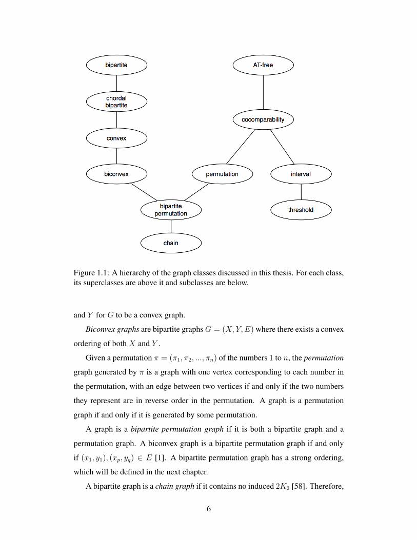
Figure 1.1: A hierarchy of the graph classes discussed in this thesis. For each class,its superclasses are above it and subclasses are below.
and Y for G to be a convex graph.
Biconvex graphs are bipartite graphsG = (X, Y,E) where there exists a convex
ordering of both X and Y .
Given a permutation π = (π1, π2, ..., πn) of the numbers 1 to n, the permutation
graph generated by π is a graph with one vertex corresponding to each number in
the permutation, with an edge between two vertices if and only if the two numbers
they represent are in reverse order in the permutation. A graph is a permutation
graph if and only if it is generated by some permutation.
A graph is a bipartite permutation graph if it is both a bipartite graph and a
permutation graph. A biconvex graph is a bipartite permutation graph if and only
if (x1, y1), (xp, yq) ∈ E [1]. A bipartite permutation graph has a strong ordering,
which will be defined in the next chapter.
A bipartite graph is a chain graph if it contains no induced 2K2 [58]. Therefore,
6
an induced subgraph of a chain graph is also a chain graph. A chain graph has a
nested neighbourhood ordering, which will be defined in the next chapter.
An asteroidal triple is a set of three vertices such that two vertices are joined
by a path that does not visit the neighbourhood of the third [14]. A graph with no
asteroidal triple is called an asteroidal-triple free (AT-free) graph. AT-free graphs
contain interval, permutation and cocomparability graphs. Bipartite permutation
graphs are exactly those AT-free graphs that are also bipartite [7].
A transitive orientation is an assignment of a direction to each edge in a graph
to produce a directed graph (V, F ) that satisfies the following condition [29]:
(a, b) ∈ F and (b, c) ∈ F implies (a, c) ∈ F , for all a, b, c ∈ V .
A graph with such an orientation is said to be transitively orientable, and is called
a comparability graph. Cocomparability graphs are graphs with transitively ori-
entable complements. They contain both permutation graphs and interval graphs.
A graph G = (V,E) is an interval graph if it is the intersection graph of inter-
vals on a line. Each vertex {v1, ..., vn} ∈ V corresponds to some interval I1, ..., In
and (vi, vj) ∈ E if and only if Ii ∩ Ij 6= ∅. The interval graphs are the graphs that
are AT-free and chordal.
A graph G = (V,E) is a threshold graph if there exists a partition of V into a
clique and an independent set, I , with an ordering of I , v1, v2, ..., vr, r = |I|, such
that NG(vi) ⊆ NG(vi+1) for i = 1...r − 1.
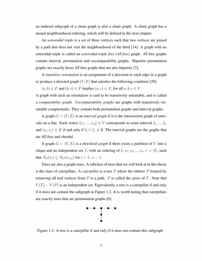
Trees are also a graph class. A subclass of trees that we will look at in this thesis
is the class of caterpillars. A caterpillar is a tree T where the subtree P formed by
removing all leaf vertices from T is a path. P is called the spine of T . Note that
V (T )− V (P ) is an independent set. Equivalently, a tree is a caterpillar if and only
if it does not contain the subgraph in Figure 1.2. It is worth noting that caterpillars
are exactly trees that are permutation graphs [6].
Figure 1.2: A tree is a caterpillar if and only if it does not contain this subgraph.
7
1.4 Problem Definitions
The minimum spanning tree problem is a classic graph theory problem, initially
presented by Czech mathematician Otakar Boruvka [5]. The problem is, given a
weighted graph G = (V,E, c), find a spanning tree T of G such that the total cost
of the edges in T is minimized over all spanning trees of G.
Problem 1.1. Minimum Spanning Tree: Given a weighted graph G = (V,E, c)
find T such that w(T ) =∑
(u,v)∈T
w(u, v) is minimized.
Boruvka’s interest in the problem began when tasked with finding the most eco-
nomical construction of the electric power network in southern Moravia [30]. While
Boruvka was the first to explicitly define a minimum spanning tree of a graph, dis-
cussions that came close to defining the problem also existed in work on anthropo-
logical classification in the early 1900s [30].
A simplified version of the algorithm presented by Boruvka is this: given a
graph G, and a tree T = (V (G), ∅), for every connected component of T , add the
shortest edge to connect that component to another connected component to E(T ).
This algorithm assumes that each edge weight is distinct.
The two most famous solutions for the minimum spanning tree problem are
Kruskal’s algorithm and Prim’s algorithm. Kruskal’s algorithm builds a minimum
spanning tree T for graph G as follows: let T = (V (G), ∅). Then, while T is not
a spanning tree of G, take the lowest weight edge (u, v) ∈ G that is not in T such
that it does not create a cycle in T , and add it to T [35]. Kruskal also gives a dual
of this algorithm, which constructs T from G by at each step removing the highest
weighted edge that does not disconnect the graph.
Prim’s algorithm chooses an arbitrary initial vertex x, and sets T = (V (G), ∅).
Then, while T is not a spanning tree, it takes the lowest weight edge (u, v) such that
u is in the same connected component as x and v is not, and adds it to T [46].
Prim published this algorithm in 1957, and it was also independently discovered
by Dijkstra in 1959 [18]. However, this solution was first discovered in 1930 by
8
Jarnık [33], in response to Boruvka’s paper: the subtitle of his publication was “On
a letter to O. Boruvka” [30]. It appears that Kruskal was the first to discover the
solution that bears his name.
Each of these algorithms runs in polynomial time, and so the minimum spanning
tree problem can be solved in polynomial time. Currently the fastest algorithm for
solving the minimum spanning tree problem runs in O(mα(m,n)) time on an n-
vertex, m-edge graph, where α is the inverse Ackermann function, and is due to
Chazelle [10].
A minimum degree spanning tree (MDST) of a connected graph G is a spanning
tree T of G such that ∆(T ) is minimum over all spanning trees of G. We denote
the minimum ∆(T ) of all spanning trees T of a graph G as ∆∗G. The subscript may
be omitted if the context is clear. An MDST of G is a k-tree with k = ∆∗G.
We consider the following problems for unweighted, undirected graphs.
Problem 1.2. Degree Constrained Spanning Tree: Given a graph G and an inte-
ger k, does G have a spanning tree T such that ∆(T ) ≤ k?
The degree constrained spanning tree problem is NP-complete, and remains NP-
complete when k is restricted to two [27]. When k = 2, this is the Hamiltonian path
problem.
Problem 1.3. Minimum Degree Spanning Tree: Given a graph G, compute the
value of ∆∗G.
The minimum degree spanning tree problem is the optimization version of the
degree constrained spanning tree problem, looking for the minimum k such that
G has a spanning tree with ∆(T ) = k. This minimum k is ∆∗G. Therefore, the
minimum degree spanning tree problem is NP-hard.
Problem 1.4. Minimum Degree Spanning Tree Construction: Given a graph G,
find a spanning tree of T of G such that ∆(T ) = ∆∗G.
9
1.5 Contributions
In this thesis, we investigate two graph classes, chain graphs and bipartite permuta-
tion graphs. In Chapter 3, we present a polynomial time algorithm for solving the
minimum degree spanning tree problem and finding an MDST in a chain graph, as
well as a formula for ∆∗G for a chain graph G.
In Chapter 4, we give some structural results for longest paths in bipartite per-
mutation graphs, and show that there exists an MDST of a given bipartite permu-
tation graph that contains no edge crossings, as well as one that contains a longest
path in the given graph. We combine these results to show that for a bipartite per-
mutation graph G, there exists an MDST of G that is a crossing-free caterpillar
containing a longest path. We also present a dynamic programming algorithm that
computes ∆∗G for a bipartite permutation graph G and finds an MDST of G, in
polynomial time.
10
Chapter 2
Background
In this section, we discuss background work related to the minimum degree span-
ning tree problem in general and on specific graph classes.
In the first part of this chapter, we present background work on the minimum
degree spanning tree problem. First, we give the complexity of problems of the
minimum degree spanning tree problem and of some related problems. Since the
minimum degree spanning tree problem is NP-hard in general, we then give some
attention to work done on approximation algorithms for the problem and some of
its variations. This review will only discuss work on undirected graphs. We also
review background work on sufficient conditions for a graph to have a k-tree, along
with the conditions for a graph to have a Hamiltonian path that inspired them.
The second part of this chapter discusses previous work that we use to assist us
in obtaining our results. We present some vertex orderings and other properties of
the bipartite graph classes introduced in the first chapter. We discuss what is known
about the complexities of problems related to the minimum degree spanning tree
problem on certain graph classes. Lastly, we introduce a number of properties of
trees that will be used in this thesis.
2.1 Complexity, Related Problems, and Variations onthe Minimum Degree Spanning Tree Problem
We now discuss some problems related to the minimum degree spanning tree prob-
lem and their complexities.
11
A Hamiltonian path in a graphG is a path that contains each vertex ofG exactly
once.
Problem 2.1. Hamiltonian Path: Given a graph G, does G have a Hamiltonian
path?
Consider the degree constrained spanning tree problem with k = 2. This is
equivalent to the Hamiltonian path problem, and so the minimum degree spanning
tree problem is a generalization of the Hamiltonian path problem. The Hamiltonian
cycle problem asks if there exists a cycle that spans G. Both the Hamiltonian path
and the Hamiltonian cycle problems are NP-complete [27]. This implies the NP-
completeness of the degree constrained spanning tree problem. In addition, Garey
and Johnson [27] give the following reduction from the Hamiltonian path problem
to the degree constrained spanning tree problem where the parameter k is a fixed
constant. Let G be a graph with at least three vertices. Construct G′ by adding
k − 2 leaves to each vertex of G. G′ has a spanning tree with maximum degree k if
and only if G has a Hamiltonian path. Thus, the degree constrained spanning tree
problem is NP-complete for any fixed k ≥ 2.
Problem 2.2. Longest Path (decision): Given a graph G and a positive integer k,
does G contain a path with k or more edges?
Problem 2.3. Longest Path (optimization): Given a graph G, what is the largest k
such that G contains a path with k edges?
If we let k = |V | − 1 in the longest path decision problem, this is the same as
the Hamiltonian path problem, and so the longest path decision problem is another
generalization of the Hamiltonian path problem. The longest path decision problem
is NP-complete [27], and so the longest path optimization problem is NP-hard. For
the purposes of this thesis, we will refer to the longest path optimization problem
as the longest path problem.
For any graph class, if the Hamiltonian path problem is NP-complete, then its
generalizations, the decision versions of the longest path problem and the degree
constrained spanning tree problem are also NP-complete. The longest path problem
and the minimum degree spanning tree problem are NP-hard on such a class.
12

We will see that the Hamiltonian path problem is polynomial time solvable
on graph classes such as interval graphs, bipartite permutation graphs, and chain
graphs. These classes are a good starting point for finding polynomial time results
for the minimum degree spanning tree problem.
We now look at some generalizations of the minimum degree spanning tree
problem on weighted graphs.
Given a weighted graph G, there are two constraints to be optimized: the max-
imum degree of any vertex in a spanning tree, and the weight of the spanning tree.
Since there may not be a minimum weight tree with the minimum maximum de-
gree, variations of this problem must involve some compromise between the weight
of the spanning tree and the maximum degree of any vertex.
Problem 2.4. Minimum Degree Minimum Spanning Tree (MDMST): Given a
weighted graph G, find the minimum maximum degree of a minimum weight span-
ning tree of G.
The MDMST problem finds the minimum weight of a spanning tree, but the
minimum maximum degree of a minimum weight spanning tree may be higher
than is possible in a spanning tree with higher weight. The MDMST problem com-
promises on the optimality of the maximum degree of a vertex in order to achieve
optimality on the weight of the tree. In the unweighted case, the MDMST problem
is the minimum degree spanning tree problem, and so it is NP-hard.
Problem 2.5. Bounded Degree Minimum Spanning Tree (BDMST): Given a
weighted graph G and a set of integer degree bounds, find a spanning tree that
satisfies the degree bounds, and has smallest possible weight.
For the BDMST problem, these degree bounds may be some constant upper-
bound B for all vertices, or each vertex v can have its own upper bound Bv. There
may also be a specified lower boundAv for each vertex v as well. If no lower bound
is specified, Av = 1 for all v is implied, since this is required in any spanning tree.
Thus, the BDMST problem finds a spanning tree T such that Av ≤ degT (v) ≤ Bv
for each vertex v and the weight of T is minimized over all spanning trees satisfying
these degree bounds. The BDMST problem is also NP-hard.
13
There are a number of other problems that are related to the minimum degree
spanning tree problem, but are not generalizations or specifications of the problem.
The following problems related to Minimum Degree Spanning Tree are also NP-
complete [27]: Maximum Leaf Spanning Tree, Steiner Tree in Graphs, Partition
into Hamiltonian Subgraphs, and Degree Bounded Connected Subgraph.
A minimum degree Steiner tree for some D ⊆ V is a minimum degree tree
in G that spans at least the vertices in D. The minimum degree spanning tree
problem is a special case of the minimum degree Steiner tree problem, when D =
V . This problem is used to obtain some of the approximation results presented in
this chapter.
The spanning tree problem is a classic problem in graph theory, and so many
variations of the problem have been studied. We will mention some problem vari-
ations here, but we will not focus on them in detail. For an extensive survey of
spanning tree problems, see [45].
The problem of finding a minimum spanning tree of a graph that has a degree
constraint on exactly one vertex in the graph is linear-time reducible to the mini-
mum spanning tree problem [26]. Additionally, if only some vertices in the graph
have degree constraints, and these vertices form an independent set, the problem is
solvable in polynomial time [39].
While the minimum degree spanning tree problem is NP-hard, finding a span-
ning tree of a graph with maximum ∆(T ) can be solved efficiently with a greedy
algorithm. For example, for a graph G = (V,E), choose v ∈ V such that
degG(v) = ∆(G). Begin constructing a maximum degree spanning tree T by
adding all edges in G that are incident on v. Continue to add edges to T until it
is a spanning tree. We have that ∆(T ) = ∆(G), and it cannot be any greater.
However, the maximization versions of other related problems are not all easy.
Finding a spanning tree of a graph with the maximum possible number of leaves is
NP-hard [22].
14
2.2 Approximations
Since the minimum degree spanning tree problem is NP-hard, much of the work
done on this problem has been in the area of approximation algorithms. We discuss
some approximation algorithms here; for a more complete review of this area, see
[48].
In this section, we review approximation algorithms for two variations of the
minimum spanning tree problem, the MDMST problem and the BDMST problem.
In the unweighted case, the MDMST problem is equivalent to the minimum degree
spanning tree problem.
2.2.1 Unweighted Approximations
We first discuss work on approximation algorithms for the minimum degree span-
ning tree problem, which is defined for unweighted graphs.
Furer and Raghavachari [24] first gave a polynomial time algorithm that returns
a spanning tree T with ∆(T ) ∈ O(∆∗+log n). The algorithm reduces the minimum
degree spanning tree problem to a maximal matching in auxiliary graphs.
In [25], Furer and Raghavachari present a better polynomial time approximation
algorithm for the minimum degree spanning tree problem, and more particularly, for
the minimum degree Steiner tree problem, that produces a Steiner tree T such that
∆(T ) ≤ ∆∗G + 1.
The algorithm presented is shown to produce a spanning tree T of G that has
∆(T ) ≤ ∆∗G + 1. Finding an upper bound on ∆∗G is easy; simply produce any
spanning tree T of G, and we know that ∆∗G ≤ ∆(T ). The proof of correctness for
this algorithm relies on a witness set to give a lower bound on ∆∗G and show that
∆∗G is within one of optimal. A witness set is a subset of the vertices of G, W ⊆ V
with |W | = w, and the removal of W from G disconnects G into t components.
Let d = dw+t−1we. Then [25] shows that ∆∗G ≥ d.
The algorithm for producing this spanning tree ofG with ∆(T ) ≤ ∆∗G+1 relies
on a series of improvements to an initial arbitrary spanning tree T . At each iteration
of the algorithm, a forest F is created from T by removing the set of vertices with
15
degree ∆(T ) and ∆(T )− 1 and their incident edges. If there is no edge in E(G)−
E(T ) that is between two components of F , the algorithm terminates. Otherwise,
choose (u, v) ∈ E(G)− E(T ) such that u and v are in different components of F ,
and consider the cycle C created by adding (u, v) to T . If there exists some vertex
w ∈ C such that degT (w) = ∆(T ), and if degT (u) ≤ ∆(T ) − 2 and degT (v) ≤
∆(T ) − 2 then w can be improved by adding (u, v) to T and removing an edge of
C that is incident on w. Each such improvement reduces the number of vertices of
T of degree ∆(T ), and can potentially decrease ∆(T ). If no further improvements
can be made, the set of vertices of degree ∆(T ) and ∆(T )− 1 is a witness set that
shows ∆(T ) ≤ ∆∗G + 1. This algorithm runs in O(mnα(m,n) log n), where α is
the inverse Ackermann function.
2.2.2 Weighted Approximations
We now discuss approximations for some variations of the minimum degree span-
ning tree problem on weighted graphs.
Two results for a more general version of the minimum degree spanning tree
problem are presented by Fischer in [23]. Here, we consider the minimum max-
imum degree over all spanning trees of a graph, ∆∗, and the minimum cost of a
spanning tree with maximum degree ∆∗, cost∗. The first is a generalization of
Furer and Raghavachari’s work in [25] to weighted graphs that produces a span-
ning tree T such that cost(T ) ≤ cost∗ and ∆(T ) ≤ k · (∆∗ + 1), where k is the
number of distinct edge weights in the graph.
The second result in [23] generalizes [24] to weighted graphs as well. It pro-
duces a spanning tree T such that cost(T ) ≤ cost∗ and ∆(T ) ∈ O(∆∗ · log n).
These algorithms rely on the notion of tree rank of a tree T , which is an array
{tn−1, ..., t1} where tk is the number of vertices in T with degree k. These rank-
ings are considered in lexicographic order. Then, a series of neutral weight edge
swaps (swapping an edge of weight c in T for another edge of weight c not in T )
are performed. A tree is considered locally optimal if there does not exist a neu-
tral weight edge swap that decreases the tree rank. If T is locally optimal, then
∆(T ) ≤ b · ∆∗ + dlogb ne for some constant b > 1. The time complexity of this
16
algorithm is O(n4+ 1ln b ).
Goemans conjectured that, given a graphG and a constant upper bound k for all
vertex degrees in a spanning tree of G, there exists a polynomial time algorithm to
find a spanning tree T such that ∆(T ) ≤ k+1 and the cost of T is at mostOPT (k),
where OPT (k) is the optimal cost of a spanning tree that satisfies the upper bound
k. Later, in [28], Goemans presented an algorithm for a version of the weighted
BDMST problem that produces a solution within two of optimal. This algorithm
considers weighted graphs with an upper and lower bound on the degree of each
vertex v. It settles a slightly weaker version of the conjecture, finding a spanning
tree with cost at most OPT (k) and ∆(T ) ≤ k + 2 [28].
Ravi and Singh [47] give a generalization of Furer and Raghavachari’s ∆∗ + 1
approximation algorithm for the BDMST problem. Their polynomial time algo-
rithm either shows that the degree bounds given in the problem statement are in-
feasible, or returns a spanning tree T such that degT (v) ≤ Bv + k where k is the
number of distinct edge costs in T . Previous approximation algorithms for these
problems used witness sets to find a lower bound on the optimal solution. Ravi and
Singh [47] instead use linear programming to give a stronger lower bound.
More recently, Singh and Lau [50] presented an algorithm for the BDMST prob-
lem that produces a spanning tree T such that weight(T ) ≤ OPT and Av − 1 ≤
degT (v) ≤ Bv + 1, for all v, where OPT is the weight of an optimal solution and
Av, Bv are the given bounds on the degree of vertex v. This result generalizes the
result in [25] to weighted graphs and proves Goemans’ conjecture correct. It is also
essentially the best possible result in polynomial time for the BDMST problem,
unless P = NP .
The BDMST problem is again considered in [9], using the methodology applied
by Edmonds to the weighted matching problem. Their first algorithm finds a tree
T of optimal cost with ∆(T ) ≤ b2−bB + logb n, b ∈ (1, 2), where B is the upper
bound for all vertex degrees in T , in polynomial time. Their second algorithm
improves on this by finding a spanning tree T of optimal cost with ∆(T ) ≤ B +
O( lognlog logn
) in quasi-polynomial time. A quasi-polynomial time algorithm is slower
than a polynomial time algorithm, but still faster than exponential time. This second
17
algorithm gets a huge improvement on the accuracy of ∆(T ), but at the expense of
being slower than polynomial time. This improvement in error on the maximum
degree is achieved using an analogy to bipartite matching, and by using augmenting
path techniques.
These approximation algorithms are for general weighted graphs which may
be considered as complete graphs with some edges having infinite weight. There
has also been work done on finding low degree, low weight spanning trees for
Euclidean graphs, where each vertex represents a point in the plane, and each pair
of points is connected by an edge with weight equal to the distance between the
points. The goal is to find a minimum weight spanning tree T such that the degree
of each vertex in bounded above by some k. This problem is explored in [37], [49],
[21], and [34]. The most recent results from [34] state that the problem is NP-hard
for 2 ≤ k ≤ 3 and polynomial time solvable for k ≥ 5. The complexity is still
unknown for k = 4, and so [34] gives an approximation algorithm that shows there
always exists a spanning tree in a such a collection of points in the plane, where the
maximum degree is 4, and the cost of this tree is at most√2+23
times the optimal
cost.
2.3 Hamiltonicity and k-trees
We discuss conditions for Hamiltonicity and for a graph to have a k-tree related
to the minimum degree of a vertex in a graph, the independence number, and the
connectivity.
One of the first sufficient conditions for Hamiltonicity of a graph is Dirac’s the-
orem, which states that for a given graph G, if δ(G) ≥ n2, then G has a Hamiltonian
cycle [19]. Ore showed that if degG(x) + degG(y) ≥ n − 1, for all x, y ∈ V such
that (x, y) /∈ E, then G has a Hamiltonian cycle [44]. This result introduces the
theme of independent sets in results for sufficient conditions for Hamiltonicity of
graphs.
Chvatal and Erdos presented further results related to independent sets and
Hamiltonicity in [11]. Let G be a graph with n ≥ 3. If G is k-connected and
18
has no independent set of size greater than k, then G has a Hamiltonian cycle. Sim-
ilarly, if G is k-connected and has no independent set of size greater than k + 1,
then G has a Hamiltonian path [11].
Bondy and Chvatal showed, for a connected graph G = (V,E) with some
(u, v) /∈ E such that degG(u) = degG(v) ≥ n − 1, G has a Hamiltonian path
if and only if G+ (u, v) has a Hamiltonian path [4].
We now discuss some generalizations of these conditions for Hamiltonicity.
These generalizations give a sufficient condition for a graph to have a k-tree.
Win generalized Ore’s result to show that if a graph G satisfies the condition in
Equation 2.1 for a given k, then G has a spanning tree T with ∆(T ) ≤ k [56].
Win’s Condition [56]:∑x∈I
deg(x) ≥ n− 1, for every k-element independent set I ⊂ V (2.1)
Win’s upper bound k on ∆∗G of a graph G also gives a lower bound on the
degrees of vertices in G. That is, δ(G) ≥ (n − 1)/k, a generalization of Dirac’s
theorem.
Win proved a conjecture of Las Vergnas in [55], which generalizes the result of
Chvatal and Erdos: every k-connected graph with independence number α ≤ k+ c
contains a spanning tree with no more than c + 1 terminal vertices. Neumann-
Lara and Rivera-Campo generalized this result to bounded degree spanning trees,
showing that if G is k-connected with α ≤ 1 + ks for s ≥ 1, then G has a spanning
tree with no vertices with degree larger than s + 1 [43]. Another result, also from
[43], gives a less tight bound on the maximum degree of the tree, but also provides
information about the number of vertices in the tree that have that maximum degree:
let G be a k-connected graph, and s ≥ 3, 0 ≤ c ≤ k. If α ≤ 1 + k(s− 1) + c then
G has a spanning tree T with no vertices with degree larger than s+ 1, and with at
most c vertices in T having degree s+ 1.
These results are interesting on dense graphs, but sparser graphs that have
Hamiltonian paths are less likely to satisfy these conditions. Czumaj and Stroth-
mann [15] looked at algorithms for a degree bounded spanning tree problem on
k-connected graphs, and also compiled results for the problem on planar graphs,
19
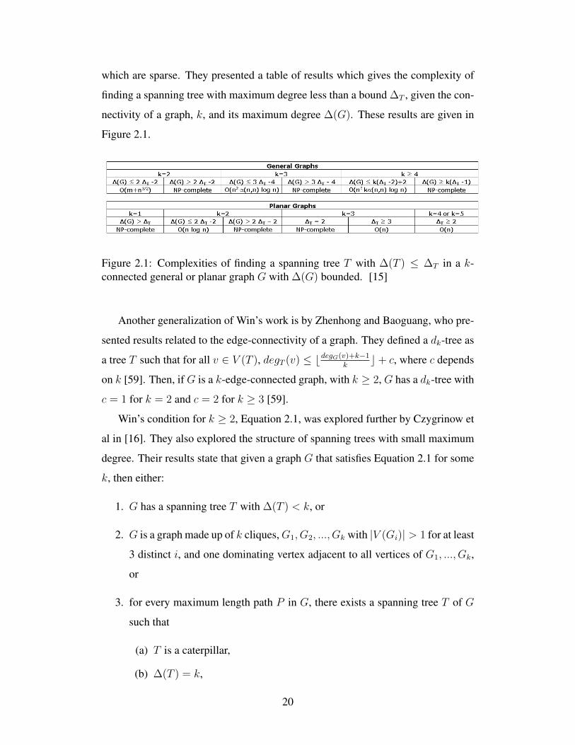
which are sparse. They presented a table of results which gives the complexity of
finding a spanning tree with maximum degree less than a bound ∆T , given the con-
nectivity of a graph, k, and its maximum degree ∆(G). These results are given in
Figure 2.1.
Figure 2.1: Complexities of finding a spanning tree T with ∆(T ) ≤ ∆T in a k-connected general or planar graph G with ∆(G) bounded. [15]
Another generalization of Win’s work is by Zhenhong and Baoguang, who pre-
sented results related to the edge-connectivity of a graph. They defined a dk-tree as
a tree T such that for all v ∈ V (T ), degT (v) ≤ bdegG(v)+k−1k
c+ c, where c depends
on k [59]. Then, if G is a k-edge-connected graph, with k ≥ 2, G has a dk-tree with
c = 1 for k = 2 and c = 2 for k ≥ 3 [59].
Win’s condition for k ≥ 2, Equation 2.1, was explored further by Czygrinow et
al in [16]. They also explored the structure of spanning trees with small maximum
degree. Their results state that given a graph G that satisfies Equation 2.1 for some
k, then either:
1. G has a spanning tree T with ∆(T ) < k, or
2. G is a graph made up of k cliques,G1, G2, ..., Gk with |V (Gi)| > 1 for at least
3 distinct i, and one dominating vertex adjacent to all vertices of G1, ..., Gk,
or
3. for every maximum length path P in G, there exists a spanning tree T of G
such that
(a) T is a caterpillar,
(b) ∆(T ) = k,
20
(c) the spine of T is P ,
(d) the set {v ∈ V |degT (v) ≥ 3} is an independent set in T .
There exists a k that satisfies Equation 2.1 for all graphs, although this k does not
necessary give a good bound on ∆∗G. Consider a graph G that is a clique Kr, r ≥ 3,
with r leaves, each adjacent to exactly one vertex in the clique. The size of the
largest independent set inG is r, but the sum of the degrees of this set is r < 2r−1.
Then k = r + 1 as there is no independent set of size r + 1. On the other hand,
regardless of the size of G, ∆∗G = 3. For large r, Equation 2.1 gives a poor bound
on ∆∗G. This bound is tighter for denser graphs, and worse for sparse graphs and
graphs with many leaves.
Figure 2.2: Two bipartite permutation graphs where Win’s condition, Equation 2.1,for a k-tree is not tight and tight, respectively.
Figure 2.2 shows two bipartite permutation graphs where Win’s condition has
different accuracy. In Figure 2.2 (a), n = 16 and the condition is satisfied at k = 10,
as there is no independent set of size 10, and there exists an independent set of size
9 with degree sum less than n − 1 (the set of all leaf vertices, for example). But
the graph itself is a caterpillar and so ∆∗G = ∆(G) = 3. So Win’s condition is not
accurate here. The graph in Figure 2.2 (b) has n = 8, and satisfies Win’s condition
at k = 3. For this graph, ∆∗G = 3, so Win’s condition is tight. These examples show
that these results of [16] will not necessarily give much information about k-trees
in bipartite permutation graphs.
Bondy and Chvatal’s work was generalized by Kishimoto and Kano for j-
connected graphs. They present three results in [38]. Let G be a j-connected
graph, for some j ≥ 1, and let k ≥ 2. First, for some (u, v) /∈ E such that
21
degG(u) + degG(v) ≥ n − 1 − (k − 2)j, then G has a spanning k-tree if and
only if G + (u, v) has a spanning k-tree. Next, for some (u, v) /∈ E such that
degG(u) + degG(v) ≥ n − k + 1, then G has a spanning k-tree if and only
if G + (u, v) has a spanning k-tree. Finally, if for all (u, v) /∈ E, we have
degG(u) + degG(v) ≥ n− 1− (k − 2)j, then G has a spanning k-tree.
2.4 Vertex Orderings and Properties of Bipartite GraphClasses
We now discuss vertex orderings for bipartite graph classes.
A convex ordering of one vertex set of a bipartite graph (assume X) is an or-
dering of the vertices of X such that for every y ∈ Y , N(y) is consecutive in the
ordering ofX . As previously mentioned, a bipartite graphG = (X, Y,E) is convex
if there exists a convex ordering of X or Y , and is biconvex if there exists a convex
ordering of both X and Y .
An ordering of the vertices X of a bipartite graph G = (X, Y,E) has the adja-
cency property if for each vertex y ∈ Y , the vertices of N(y) are consecutive in the
ordering of X , and has the enclosure property if for every pair of vertices u, v ∈ Y ,
if N(u) ⊂ N(v), then N(v)−N(u) is consecutive in the ordering of X .
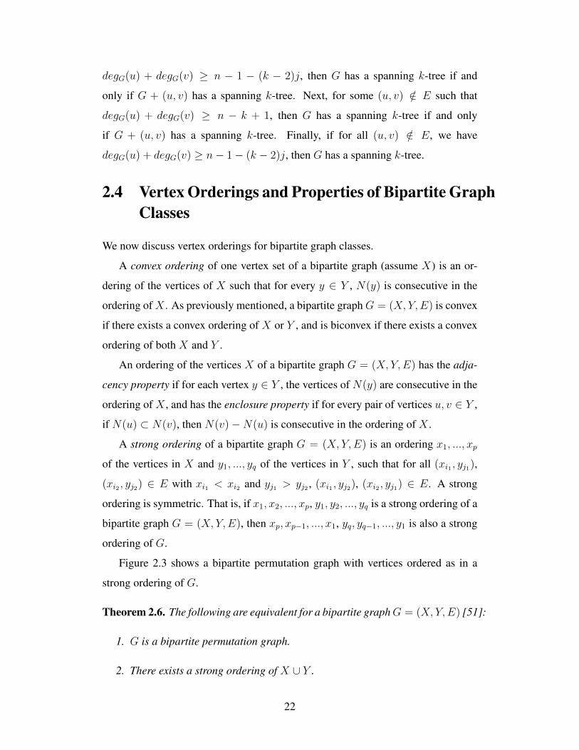
A strong ordering of a bipartite graph G = (X, Y,E) is an ordering x1, ..., xp
of the vertices in X and y1, ..., yq of the vertices in Y , such that for all (xi1 , yj1),
(xi2 , yj2) ∈ E with xi1 < xi2 and yj1 > yj2 , (xi1 , yj2), (xi2 , yj1) ∈ E. A strong
ordering is symmetric. That is, if x1, x2, ..., xp, y1, y2, ..., yq is a strong ordering of a
bipartite graph G = (X, Y,E), then xp, xp−1, ..., x1, yq, yq−1, ..., y1 is also a strong
ordering of G.
Figure 2.3 shows a bipartite permutation graph with vertices ordered as in a
strong ordering of G.
Theorem 2.6. The following are equivalent for a bipartite graphG = (X, Y,E) [51]:
1. G is a bipartite permutation graph.
2. There exists a strong ordering of X ∪ Y .
22
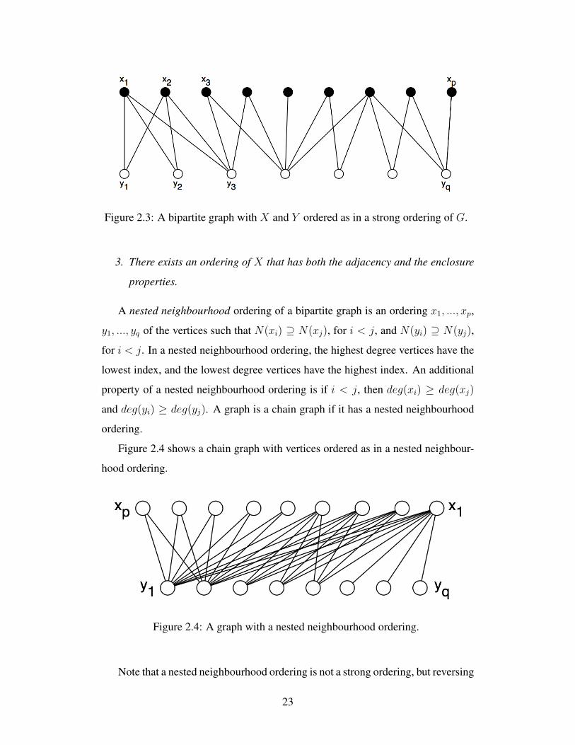
Figure 2.3: A bipartite graph with X and Y ordered as in a strong ordering of G.
3. There exists an ordering of X that has both the adjacency and the enclosure
properties.
A nested neighbourhood ordering of a bipartite graph is an ordering x1, ..., xp,
y1, ..., yq of the vertices such that N(xi) ⊇ N(xj), for i < j, and N(yi) ⊇ N(yj),
for i < j. In a nested neighbourhood ordering, the highest degree vertices have the
lowest index, and the lowest degree vertices have the highest index. An additional
property of a nested neighbourhood ordering is if i < j, then deg(xi) ≥ deg(xj)
and deg(yi) ≥ deg(yj). A graph is a chain graph if it has a nested neighbourhood
ordering.
Figure 2.4 shows a chain graph with vertices ordered as in a nested neighbour-
hood ordering.
Figure 2.4: A graph with a nested neighbourhood ordering.
Note that a nested neighbourhood ordering is not a strong ordering, but reversing
23
the ordering of either X or Y gives a strong ordering. That is, if x1, ..., xp, y1, ..., yq
is a nested neighbourhood ordering, then xp, ..., x1, y1, ..., yq is a strong ordering.
We use the strong ordering property of some bipartite graphs to introduce more
definitions and properties for these graphs.
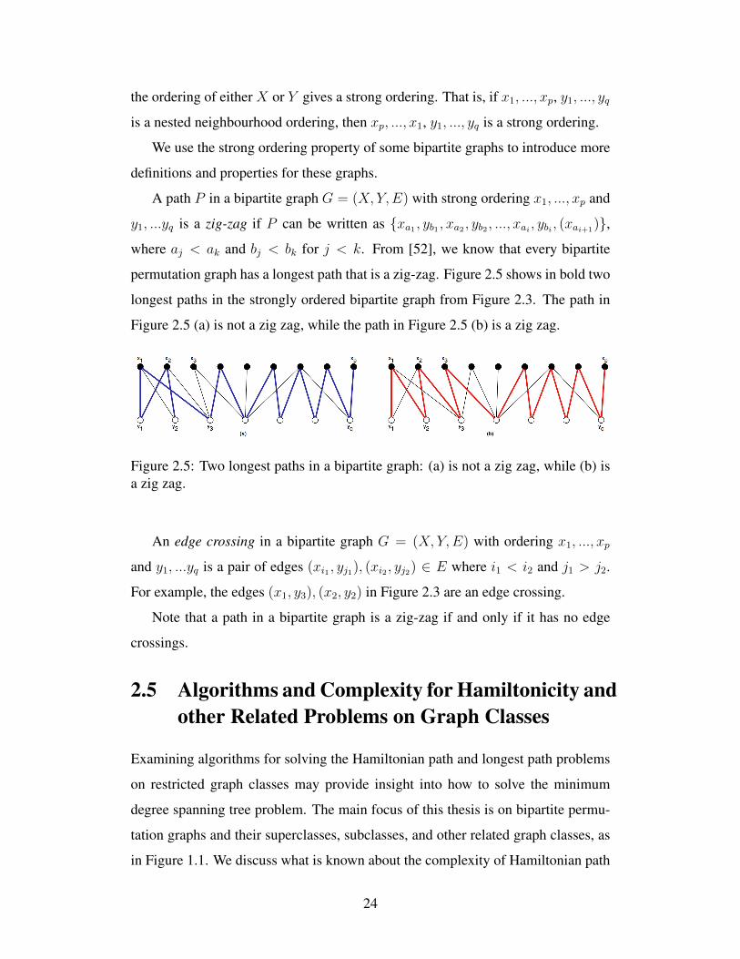
A path P in a bipartite graph G = (X, Y,E) with strong ordering x1, ..., xp and
y1, ...yq is a zig-zag if P can be written as {xa1 , yb1 , xa2 , yb2 , ..., xai , ybi , (xai+1)},
where aj < ak and bj < bk for j < k. From [52], we know that every bipartite
permutation graph has a longest path that is a zig-zag. Figure 2.5 shows in bold two
longest paths in the strongly ordered bipartite graph from Figure 2.3. The path in
Figure 2.5 (a) is not a zig zag, while the path in Figure 2.5 (b) is a zig zag.
Figure 2.5: Two longest paths in a bipartite graph: (a) is not a zig zag, while (b) isa zig zag.
An edge crossing in a bipartite graph G = (X, Y,E) with ordering x1, ..., xp
and y1, ...yq is a pair of edges (xi1 , yj1), (xi2 , yj2) ∈ E where i1 < i2 and j1 > j2.
For example, the edges (x1, y3), (x2, y2) in Figure 2.3 are an edge crossing.
Note that a path in a bipartite graph is a zig-zag if and only if it has no edge
crossings.
2.5 Algorithms and Complexity for Hamiltonicity andother Related Problems on Graph Classes
Examining algorithms for solving the Hamiltonian path and longest path problems
on restricted graph classes may provide insight into how to solve the minimum
degree spanning tree problem. The main focus of this thesis is on bipartite permu-
tation graphs and their superclasses, subclasses, and other related graph classes, as
in Figure 1.1. We discuss what is known about the complexity of Hamiltonian path
24
and longest path on the classes shown in Figure 1.1.
We start with one of the highest level superclasses of bipartite permutation
graphs as shown in Figure 1.1, bipartite graphs. Moon and Moser explored the
Hamiltonicity of bipartite graphs in [41], and showed both the Hamiltonian cycle
and Hamiltonian path problems remain NP-complete on bipartite graphs.
The most basic necessary condition for a bipartite graph G = (X, Y,E) to
have a Hamiltonian cycle is that p = q. For a Hamiltonian path to exist in a bi-
partite graph, we must have |p − q| ≤ 1. Moon and Moser [41] present some
sufficient conditions for the existence of a Hamiltonian cycle in a bipartite graph.
Let p = |X| = |Y | for the following results. A bipartite graph G = (X, Y,E) has a
Hamiltonian cycle if for any non-empty subset F of X ∪ Y with |F | = k ≤ p2,
such that for every xi ∈ F , degG(xi) ≤ k, then every vertex yj ∈ Y with
degG(yj) ≤ p− k, yj is adjacent in G to some vertex in F . The same holds with X
and Y reversed. A corollary to this is that for a bipartite graph G = (X, Y,E), if
for each k, 1 ≤ k ≤ p2, the number of vertices x ∈ X such that degG(x) ≤ k is less
than k, and the same for all y ∈ Y , then G has a Hamiltonian cycle. This can also
be stated as, if G has degG(x) + degG(y) > p for all x, y ∈ G such that (x, y) /∈ E,
then G has a Hamiltonian cycle.
Chordal bipartite graphs are contained in bipartite graphs, and contain bipartite
permutation graphs. Muller [42] gives a reduction from SAT to both Hamiltonian
cycle and Hamiltonian path in chordal bipartite graphs.
A Hamiltonian cycle can be found in a convex graph in polynomial time, as
shown in [42]. Keil showed that there exists a linear time algorithm for finding a
Hamiltonian cycle in an interval graph [36], and [42] presents an O(n2) reduction
from a convex bipartite graph G = (X, Y,E) to an interval graph G′ such that there
exists a Hamiltonian cycle in G′ if and only if there exists a Hamiltonian cycle in
G. The reduction is as follows: assume X is convex. Let G′ = (X ∪ Y,E ∪
{(y1, y2)|NG(y1)∩NG(y2) 6= ∅}). G′ is now an interval graph and Keil’s algorithm
can find a Hamiltonian cycle C in linear time. Since X is an independent set, all
edges in the cycle must be in E. Therefore C is also a Hamiltonian cycle in G.
Muller shows that the Hamiltonian path problem can be solved in O(n2) time
25
for convex and biconvex graphs. The complexity of the longest path problem is
unknown for these classes [52].
A number of polynomial time results for problems related to the minimum de-
gree spanning tree problem are known for bipartite permutation graphs. Spinrad,
Brandstadt and Stewart [51] present conditions for a bipartite permutation graph
G = (X, Y,E) to have a Hamiltonian path or Hamiltonian cycle.
Theorem 2.7. [51] Let G = (X, Y,E) be a bipartite permutation graph contain-
ing a Hamiltonian path beginning at x ∈ X . Let x1, ..., xp and y1, ...yq be a strong
ordering of G. Then (x1, y1, x2, y2, ..., xp, yp) or (x1, y1, x2, y2, ..., xp−1, yq, xp) is
also a Hamiltonian path in G, where x1, x2, ..., xp, y1, y2, ..., yq is a strong or-
dering of G. Similarly, if G has a Hamiltonian path beginning at some y ∈ Y ,
then (y1, x1, y2, x2, ..., yq, xq) or (y1, x1, y2, x2, ..., yq−1, xp, yq) is also a Hamilto-
nian path.
Therefore, determining if a bipartite permutation graph has a Hamiltonian path
reduces to just determining if it contains one of the paths in Theorem 2.7. Uehara
and Uno give a linear time algorithm to solve the longest path problem on bipartite
permutation graphs [53].
The results for the Hamiltonian path problem on bipartite permutation graphs
apply to chain graphs, which are a subclass of bipartite permutation graphs. The
longest path problem can be solved in O(n) time on chain graphs, as in [53].
The complexity of the minimum degree spanning tree problem was not known
for any graph class between chain graphs and convex bipartite graphs, prior to our
work.
The other highest level superclass of bipartite permutation graphs that we will
discuss here are AT-free graphs. The complexity of the Hamiltonian cycle and
Hamiltonian path problems on AT-free graphs is unknown [2]. It is also unknown
for the minimum degree spanning tree problem, and for longest path.
Both the Hamiltonian path problem is solvable in polynomial time for cocom-
parability graphs [17]. Recently, Mertzios and Corneil [40] showed that the longest
path problem is also polynomial time solvable for cocomparability graphs. There-
fore, the cocomparability graphs and their subclasses provide an interesting starting
26
point for exploring the minimum degree spanning tree problem. The Hamiltonian
path problem and longest path problem can be solved in polynomial time for per-
mutation graphs, since all permutation graphs are cocomparability graphs.
It is also useful to consider graph classes such as interval graphs and threshold
graphs, although they are not directly related to bipartite permutation graphs. As we
have seen when discussing the Hamiltonicity of convex bipartite graphs, there is a
connection between convex bipartite graphs and interval graphs. Threshold graphs
are very similar to chain graphs, and can be thought of as a chain graph with edges
added to either X or Y of a chain graph to form a clique. Both of these classes also
have polynomial time results for problems related to the minimum degree spanning
tree problem.
As previously mentioned, Keil showed there is a linear time solution for the
Hamiltonian path problem on interval graphs [36]. Uehara and Uno showed that the
longest path problem on interval graphs can be reduced to the longest path problem
on convex bipartite graphs [52]. Recently, Ioannidou et al. gave a O(n4) algorithm
to solve the longest path problem on interval graphs [32].
Harary and Peled give a necessary and sufficient condition for a threshold graph
to have a Hamiltonian cycle [31]. This condition gives a lower bound on the degree
of each vertex in G that holds if and only if G has a Hamiltonian cycle. A condition
for a Hamiltonian path is not given, but it is easy to see how the Hamiltonian cycle
condition might be altered for the Hamiltonian path problem. Uehara and Uno also
showed the longest path problem has a linear time solution for threshold graphs
[52].
The results discussed in this section are summarized in Table 2.1. Note that there
is no citation for the NP-hard results for the longest path problem where the Hamil-
tonian path problem is known to be NP-complete since a solution to the longest
path problem gives a solution to the Hamiltonian path problem.
27

Graph Class Hamiltonian Path Longest Pathbipartite NP-c [41] NP-hardchordal bipartite NP-c [42] NP-hardconvex O(n2) [42] unknownbiconvex O(n2) [42] unknownbipartite permutation O(n) [51] O(n) [53]chain O(n) [51] O(n) [53]AT-free unknown unknowncocomparability O(n2) [17] O(n4) [40]permutation O(n2) [17] O(n4) [40]interval O(n) [36] O(n4) [32]threshold O(n) [31] O(n) [52]
Table 2.1: Complexity results for the Hamiltonian path and longest path problemsfor certain graph classes
2.6 Properties of Trees
We make use of properties of trees in many of the proofs in this thesis. In particu-
lar, we use these properties to show that trees we construct from other trees using
particular techniques retain the properties of the initial trees.
Theorem 2.8 gives several characteristics of trees.
Theorem 2.8. For a graph G, the following are equivalent [54]:
1. G is connected and has no cycles.
2. G is connected and has n− 1 edges.
3. G has n− 1 edges and no cycles.
4. G has no cycles and has, for each u, v ∈ V (G), exactly one (u, v)-path.
5. G is a tree.
There are many other properties of trees and spanning trees that we make use of
in this thesis. For these and other properties, see [54].
We know some specific things about the connectivity and colouring of trees.
Adding one edge anywhere in a tree forms a cycle. Every non-leaf vertex in a tree
28

is a cut vertex, and every edge in a tree is a cut edge. Since trees have no cycles,
they are bipartite.
Every connected graph has a spanning tree, and a graph that is a tree has exactly
one spanning tree. A path is a tree with maximum degree two.
Let T and T ′ be two distinct spanning trees of a connected graph G. Let e be
an edge in E(T )− E(T ′). Then there exists an edge e′ in E(T ′)− E(T ) such that
T − e+ e′ is a spanning tree of G.
29
Chapter 3
Chain Graphs
As previously defined, a bipartite graph G = (X, Y,E) is a chain graph if it has no
induced 2K2, and a chain graph has an ordering of its vertices x1, ..., xp, y1, ..., yq
that is a nested neighbourhood ordering. That is, N(xi) ⊇ N(xj), for i < j, and
N(yi) ⊇ N(yj), for i < j. In this chapter, we assume that |X| ≥ |Y |; that is, that
X is the larger side of the graph.
Let G = (X, Y,E) be a chain graph with nested neighbourhood ordering
x1, ..., xp and y1, ..., yq. Recall that therefore xp, ..., x1, y1, ..., yq is a strong or-
dering of G. By the definition of the nested neighbourhood ordering, x1 is the high
degree vertex in X and y1 is the high degree vertex in Y . The nested neighbour-
hood ordering also has the property that if i < j, then deg(xi) ≥ deg(xj) and
deg(yi) ≥ deg(yj). Since G is a chain graph, x1 dominates Y and y1 dominates X .
The vertices in X will be drawn with xp on the left and x1 on the right. The vertices
in Y will be drawn with y1 on the left and yq on the right.
For the purposes of this work, we will only consider chain graphs that are con-
nected. A disconnected graph does not have an MDST.
In this chapter, we give a degree condition for a chain graph to have a Hamilto-
nian path, and present an algorithm to find a spanning tree with a certain maximum
degree in a chain graph. We then show that this spanning tree is an MDST of G.
30
3.1 A Degree Condition for Hamiltonian Chain Graphs
We give an exact condition for a chain graph to have a Hamiltonian path. Equiva-
lently, the condition holds if and only if a chain graph has an MDST with ∆∗G = 2.
Chain graphs are a subclass of bipartite permutation graphs, and we make use
of Theorem 2.7 in our proof.
Theorem 3.1. Let G = (X, Y,E) be a chain graph with nested neighbourhood
ordering x1, ..., xp and y1, ...yq. Then G has a Hamiltonian path if and only if one
of the following conditions holds:
(1) p = q, and
degG(xi) ≥ p− i+ 1, for all xi ∈ X , and
degG(yj) ≥ p− j + 1, for all yj ∈ Y .
(2) p = q + 1, and
degG(xi) ≥ p− i+ 1, 2 ≤ i ≤ p, degG(x1) = q, and
degG(yj) ≥ q − j + 2, for all yj ∈ Y .
Proof. We first show that these conditions are sufficient forG to have a Hamiltonian
path.
Observation: Since G is a chain graph, we know x1 dominates Y and y1
dominates X , and the neighbourhood of each vertex is consecutive in the nested
neighbourhood ordering. We observe that, if degG(xi) ≥ dx, then NG(xi) ⊇
{y1, ..., ydx}. Similarly, if degG(yj) ≥ dy, then NG(yj) ⊇ {x1, ..., xdy}.
Recall that if x1, ..., xp, y1, ..., yq is a nested neighbourhood ordering, then
xp, ..., x1, y1, ..., yq is a strong ordering.
Assume condition (1) holds. We show that G has the Hamiltonian path xp, y1,
xp−1, y2, ..., x1, yp. We now show that condition (1) guarantees we have this path.
We first show that condition (1) guarantees we have each (xi, yj) edge in this
path. Note that we can rewrite the indices in that path xp, y1, xp−1, y2, ..., x1, yp to
be xp, yp−p+1, xp−1, yp−(p−1)+1, ..., x1, yp−1+1. Thus, we want to show that for each
xi, the edge (xi, yp−i+1) is in E. By our assumption that condition (1) holds, then
31
degG(xi) ≥ p−i+1, and by our earlier observation, thenNG(xi) ⊇ {y1, ..., yp−i+1}.
Therefore, (xi, yp−i+1) ∈ E for 1 ≤ i ≤ p.
It remains to be shown that (yj, xp−j) ∈ E for all 1 ≤ j < p. By the assumption
that condition (1) holds, degG(yj) ≥ p− j + 1, and by our earlier observation, then
NG(yj) ⊇ {x1, ..., xp−j+1}, and so (yj, xp−j) ∈ E for 1 ≤ j < p.
Therefore, if condition (1) holds, then G has a Hamiltonian path.
Now assume condition (2) holds. Using the same argument as in the proof for
condition (1), we see that (xi, yp−i+1) ∈ E for 2 ≤ i ≤ p, and (yj, xp−j) ∈ E for
1 ≤ j ≤ q. Therefore, G has the Hamiltonian path xp, y1, xp−1, y2, ..., x2, yp−1, x1.
We now show that these conditions are necessary for G to have a Hamiltonian
path.
Assume p = q and condition (1) does not hold for all vertices. By Theorem 2.7,
if neither xp, y1, xp−1, y2, ..., x1, yp nor y1, xp, y2, xp−1, ..., yp, x1 is a Hamiltonian
path of G, then G has no Hamiltonian path. If condition (1) does not hold, then
there exists a vertex xi such that degG(xi) < p − i + 1, or a vertex yj such that
degG(yj) < p− j + 1.
If degG(xi) < p− i+1, then NG(xi) ⊆ {y1, ..., yp−i}. Therefore, (xi, yp−i+1) /∈
E. This edge is in both xp, y1, xp−1, y2, ..., x1, yp and y1, xp, y2, xp−1, ..., yp, x1,
and therefore G does not have a Hamiltonian path. An equivalent argument can be
made if degG(yj) < p− j + 1.
We can also, by the same argument, see that if p = q + 1 and condition (2) is
not satisfied for some vertex, then G does not have a Hamiltonian path.
Therefore, the conditions are necessary and sufficient, and so the theorem holds.
3.2 A Minimum Degree Spanning Tree ConstructionAlgorithm for Chain Graphs
We present an algorithm that constructs a spanning tree with a certain maximum
degree on a chain graph. Later, we will show that this algorithm solves the minimum
degree spanning tree problem and the minimum degree spanning tree construction
32
problem on chain graphs.
3.2.1 Algorithm
LetG = (X, Y,E) be a chain graph with a nested neighbourhood ordering x1, ..., xp
and y1, ..., yq. We present an algorithm to construct T , a spanning tree of G.
The edges of T will be determined by partitioning G into subgraphs, construct-
ing spanning trees on the subgraphs, and then connecting the resulting components.
We define a part to be one of these subgraphs. The parts will be chosen using a
formula that finds a set of vertices in either X or Y of the unpartitioned portion of
G such that each vertex in this set has degree less than or equal to some value, and
the size of this set divided by the size of its neighbourhood is maximum.
As we construct the partition of G, each part will consist of consecutive sets of
vertices and will be chosen from one end of the unpartitioned portion of G. The
maximum part in the unpartitioned portion of G may have its larger vertex set from
either X or Y . Since every induced subgraph of a chain graph is also a chain graph,
each part is a chain graph. As stated at the beginning of this chapter, we assume
|X| ≥ |Y |. Therefore we will assume that |X(C)| > |Y (C)|, and so there may
exist a part C of G where X(C) ⊂ Y (G) and Y (C) ⊂ X(G). Through the rest of
the chapter, we will refer to theX and Y sides of each part. Note that these labels in
the part do not necessarily correspond to X and Y in G. For a given part C, X(C)
is the larger side of C.
We use four algorithms to construct this spanning tree for a chain graph G.
ChainGraphMDST is Algorithm 1, Partition is Algorithm 2, PartMDST is Algo-
rithm 3, and ComputeRatios is Algorithm 4. The algorithms can be found at the
end of this subsection, and are further explained and proved correct in Subsection
3.2.2. Later in the chapter, we show these algorithms solve the minimum degree
spanning tree problem.
We define the following values and ratios for use in the algorithms and in The-
orem 3.5:
For a chain graph G = (X, Y,E), let k be the number of distinct vertex degrees
in X and let l be the number of distinct vertex degrees in Y . Let a1, ..., ak be the
33
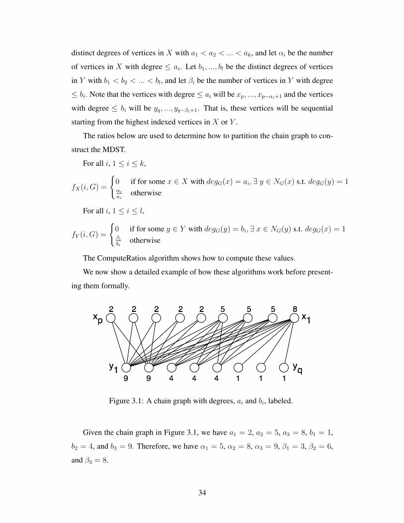
distinct degrees of vertices in X with a1 < a2 < ... < ak, and let αi be the number
of vertices in X with degree ≤ ai. Let b1, ..., bl be the distinct degrees of vertices
in Y with b1 < b2 < ... < bl, and let βi be the number of vertices in Y with degree
≤ bi. Note that the vertices with degree≤ ai will be xp, ..., xp−αi+1 and the vertices
with degree ≤ bi will be yq, ..., yq−βi+1. That is, these vertices will be sequential
starting from the highest indexed vertices in X or Y .
The ratios below are used to determine how to partition the chain graph to con-
struct the MDST.
For all i, 1 ≤ i ≤ k,
fX(i, G) =
{0 if for some x ∈ X with degG(x) = ai,∃ y ∈ NG(x) s.t. degG(y) = 1αi
aiotherwise
For all i, 1 ≤ i ≤ l,
fY (i, G) =
{0 if for some y ∈ Y with degG(y) = bi,∃ x ∈ NG(y) s.t. degG(x) = 1βibi
otherwise
The ComputeRatios algorithm shows how to compute these values.
We now show a detailed example of how these algorithms work before present-
ing them formally.
Figure 3.1: A chain graph with degrees, ai and bi, labeled.
Given the chain graph in Figure 3.1, we have a1 = 2, a2 = 5, a3 = 8, b1 = 1,
b2 = 4, and b3 = 9. Therefore, we have α1 = 5, α2 = 8, α3 = 9, β1 = 3, β2 = 6,
and β3 = 8.
34
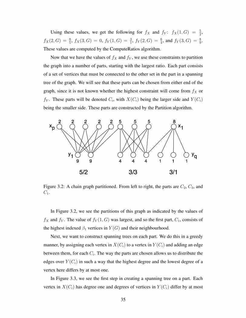
Using these values, we get the following for fX and fY : fX(1, G) = 52,
fX(2, G) = 85, fX(3, G) = 0, fY (1, G) = 3
1, fY (2, G) = 6
4, and fY (3, G) = 8
9.
These values are computed by the ComputeRatios algorithm.
Now that we have the values of fX and fY , we use these constraints to partition
the graph into a number of parts, starting with the largest ratio. Each part consists
of a set of vertices that must be connected to the other set in the part in a spanning
tree of the graph. We will see that these parts can be chosen from either end of the
graph, since it is not known whether the highest constraint will come from fX or
fY . These parts will be denoted Ci, with X(Ci) being the larger side and Y (Ci)
being the smaller side. These parts are constructed by the Partition algorithm.
Figure 3.2: A chain graph partitioned. From left to right, the parts are C2, C3, andC1.
In Figure 3.2, we see the partitions of this graph as indicated by the values of
fX and fY . The value of fY (1, G) was largest, and so the first part, C1, consists of
the highest indexed β1 vertices in Y (G) and their neighbourhood.
Next, we want to construct spanning trees on each part. We do this in a greedy
manner, by assigning each vertex in X(Ci) to a vertex in Y (Ci) and adding an edge
between them, for each Ci. The way the parts are chosen allows us to distribute the
edges over Y (Ci) in such a way that the highest degree and the lowest degree of a
vertex here differs by at most one.
In Figure 3.3, we see the first step in creating a spanning tree on a part. Each
vertex in X(Ci) has degree one and degrees of vertices in Y (Ci) differ by at most
35
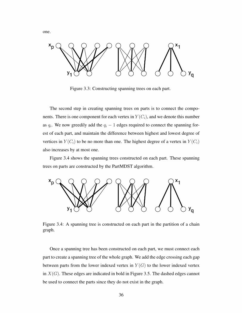
one.
Figure 3.3: Constructing spanning trees on each part.
The second step in creating spanning trees on parts is to connect the compo-
nents. There is one component for each vertex in Y (Ci), and we denote this number
as qi. We now greedily add the qi − 1 edges required to connect the spanning for-
est of each part, and maintain the difference between highest and lowest degree of
vertices in Y (Ci) to be no more than one. The highest degree of a vertex in Y (Ci)
also increases by at most one.
Figure 3.4 shows the spanning trees constructed on each part. These spanning
trees on parts are constructed by the PartMDST algorithm.
Figure 3.4: A spanning tree is constructed on each part in the partition of a chaingraph.
Once a spanning tree has been constructed on each part, we must connect each
part to create a spanning tree of the whole graph. We add the edge crossing each gap
between parts from the lower indexed vertex in Y (G) to the lower indexed vertex
in X(G). These edges are indicated in bold in Figure 3.5. The dashed edges cannot
be used to connect the parts since they do not exist in the graph.
36
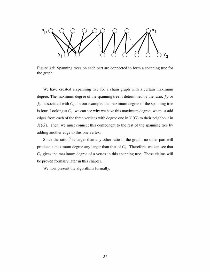
Figure 3.5: Spanning trees on each part are connected to form a spanning tree forthe graph.
We have created a spanning tree for a chain graph with a certain maximum
degree. The maximum degree of the spanning tree is determined by the ratio, fX or
fY , associated with C1. In our example, the maximum degree of the spanning tree
is four. Looking at C1, we can see why we have this maximum degree: we must add
edges from each of the three vertices with degree one in Y (G) to their neighbour in
X(G). Then, we must connect this component to the rest of the spanning tree by
adding another edge to this one vertex.
Since the ratio 31
is larger than any other ratio in the graph, no other part will
produce a maximum degree any larger than that of C1. Therefore, we can see that
C1 gives the maximum degree of a vertex in this spanning tree. These claims will
be proven formally later in this chapter.
We now present the algorithms formally.
37

Algorithm 1: ChainGraphMDSTInput: A chain graph G = (X, Y,E) with |X| ≥ |Y |Output: A spanning tree T of G
// initialize T to contain the vertices of G and noedges
T = (X, Y, ∅);// G′ is the unpartitioned portion of GG′ ← G;i← 1;while G′ 6= ∅ do
// Ci is the next part of G′
Ci ← Partition(G′);// build an MDST for Ci and add these edges to TT ← T ∪ PartMDST(Ci);G′ ← G′ − Ci;i← i+ 1;
endr ← i− 1;// connect the components of T from left to right
in a drawing of GC = an ordering of the parts Ci such that Cj < Ck if Cj is to the left of Ck ina drawing of G;// j is the index of a part in the ordering Cforeach j = 1...r − 1 do
a← min{k |xk ∈ X(G)∩C[j]};b← max{k | yk ∈ Y (G)∩C[j]};E(T )← E(T ) ∪ {(xa−1, yb)};
end
38
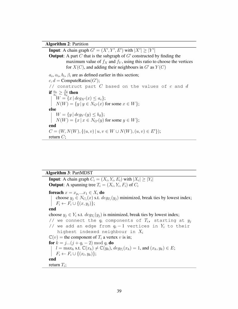
Algorithm 2: PartitionInput: A chain graph G′ = (X ′, Y ′, E ′) with |X ′| ≥ |Y ′|Output: A part C that is the subgraph of G′ constructed by finding the
maximum value of fX and fY , using this ratio to choose the verticesfor X(C), and adding their neighbours in G′ as Y (C)
ai, αi, bi, βi are as defined earlier in this section;c, d = ComputeRatios(G′);// construct part C based on the values of c and d
if αc
ac≥ βd
bdthen
W = {x | degX′(x) ≤ ac};N(W ) = {y | y ∈ NG′(x) for some x ∈ W};
elseW = {y | degY ′(y) ≤ bd};N(W ) = {x |x ∈ NG′(y) for some y ∈ W};
endC = (W,N(W ), {(u, v) |u, v ∈ W ∪N(W ), (u, v) ∈ E ′});return C;
Algorithm 3: PartMDSTInput: A chain graph Ci = (Xi, Yi, Ei) with |Xi| ≥ |Yi|Output: A spanning tree Ti = (Xi, Yi, Fi) of Ci
foreach x = xpi ...x1 ∈ Xi dochoose yj ∈ NCi
(x) s.t. degTi(yj) minimized, break ties by lowest index;Fi ← Fi ∪ {(x, yj)};
endchoose yj ∈ Yi s.t. degTi(yj) is minimized, break ties by lowest index;// we connect the qi components of Ti, starting at yj// we add an edge from qi − 1 vertices in Yi to their
highest indexed neighbour in Xi
C(v) = the component of Ti a vertex v is in;for k = j...(j + qi − 2) mod qi do
l = maxh s.t. C(xh) 6= C(yk), degTi(xh) = 1, and (xh, yk) ∈ E;Fi ← Fi ∪ {(xl, yk)};
endreturn Ti;
39
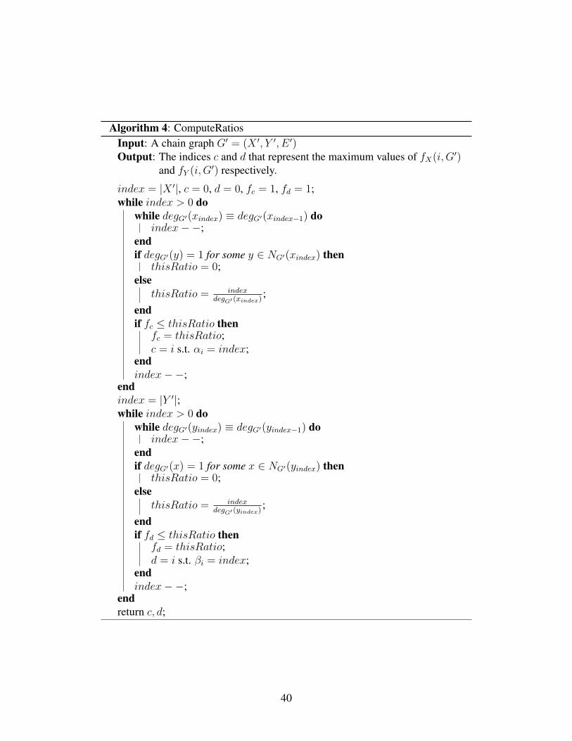
Algorithm 4: ComputeRatiosInput: A chain graph G′ = (X ′, Y ′, E ′)Output: The indices c and d that represent the maximum values of fX(i, G′)
and fY (i, G′) respectively.
index = |X ′|, c = 0, d = 0, fc = 1, fd = 1;while index > 0 do
while degG′(xindex) ≡ degG′(xindex−1) doindex−−;
endif degG′(y) = 1 for some y ∈ NG′(xindex) then
thisRatio = 0;else
thisRatio = indexdegG′ (xindex)
;endif fc ≤ thisRatio then
fc = thisRatio;c = i s.t. αi = index;
endindex−−;
endindex = |Y ′|;while index > 0 do
while degG′(yindex) ≡ degG′(yindex−1) doindex−−;
endif degG′(x) = 1 for some x ∈ NG′(yindex) then
thisRatio = 0;else
thisRatio = indexdegG′ (yindex)
;endif fd ≤ thisRatio then
fd = thisRatio;d = i s.t. βi = index;
endindex−−;
endreturn c, d;
40
3.2.2 Proof of Correctness
We first give some further explanation of the algorithms presented in the previous
subsection. ComputeRatios computes the values of fX and fY to be used by Pariti-
ton.
Partition finds the most constraining part of a chain graph, that is the part of
the graph that has the largest ratio fX or fY . PartMDST adds edges from the larger,
constraining side of a part to the smaller side, pairing each vertex inXi with a vertex
in Yi, where i is the part index. (We note that Xi and Yi in a part may be reversed
from X and Y in G, depending on how the partition was chosen.) This results in a
forest of qi components. Another qi − 1 edges must be added to finish a spanning
tree on the partition.
ChainGraphMDST takes the spanning trees constructed by PartMDST, which
result in r components, where r is the number of parts in the final partition of G.
The spanning trees for each part are then connected to their adjacent parts, in a way
to avoid increasing ∆(T ) unless necessary.
Since the definitions of fX(i, G) and fY (i, G) ensure the part with the maximum
ratio does not contain leaves in its smaller side, we can assume that for each part
Ci, there are no vertices in y ∈ Yi with degCi(y) = 1.
We now show that these algorithms construct a spanning tree with a particular
maximum degree of a chain graph G.
Lemma 3.2. Immediately following the first loop of the PartMDST algorithm and
before the second loop, there exists some k, 1 ≤ k < qi, such that degTi(yj) = dpiqie
for all 1 ≤ j ≤ k and degTi(yj) = bpiqic for all k < j ≤ qi.
Proof. We first show that degTi(yj) > degTi(yk) implies j < k. Since G is a
chain graph, NG(yj) ⊇ NG(yk) if j < k. If degTi(yk) > degTi(yj), then there was
some vertex in NG(yk) that was paired to yk instead of yj . But since we break ties
by lowest index, and j < k, then we should have made that vertex adjacent to yj
instead, a contradiction. Therefore degTi(yj) > degTi(yk) implies j < k.
By the generalized pigeonhole principle, if we are connecting pi vertices of Xi
to qi vertices of Yi, then the maximum degree of a vertex in Yi is at least dpiqie. In
41
fact, the maximum degree of a vertex in Yi is at least the ceiling of the maximum
ratio inside this part. Since Ci was chosen as the part that maximized the ratio, this
is dpiqie. So the maximum vertex degree in Yi in Ti after the pairing will be at least
dpiqie.
Assume the maximum degree of some vertex in Yi of Ti is larger than dpiqie. That
is, there exists y ∈ Yi s.t. degTi(y) ≥ dpiqie + 1 > dpi
qie. When an edge is added
from a vertex x ∈ Xi to a vertex in Yi whose degree is already dpiqie, then all other
neighbours of x in Yi have degree at least dpiqie as well.
When we try to add this new edge, the total degree ofNTi(x) is≥ |NTi(x)|∗dpiqie,
and, since we have a vertex x ∈ X that current does not have a neighbour in Ti,
|NTi(x)| ∗dpiqie < |NTi(NTi(x))|. Equivalently, |NTi
(NTi(x))|
|NTi(x)| > dpi
qie. Therefore there
is a larger ratio in Ci and the part would have been chosen differently. But since
this part was chosen, we have a contradiction. Therefore, the maximum degree of
any vertex in Yi of Ti is dpiqie.
Now we show that the minimum degree of any vertex in Yi of Ti at this point is
bpiqic. Assume there exists a vertex with degree in Ti less than bpi
qic. Since we know
that higher indexed vertices in Yi will have degrees no larger than the lower indexed
vertices, we can say that degTi(yqi) < bpiqic. Let Dqi be the set of vertices in Yi that
have the same degree in G as yqi (including yqi). SinceG is a chain graph, we know
that NCi(Dqi) = NCi
(yqi).
Since we paired each vertex in Xi of Ti to its lowest degree neighbour in Ci,
breaking ties by lowest index, if there is a vertex inDqi that has degree less than bpiqic
in Ti, then the maximum degree in Ti of a vertex in Dqi differs from the minimum
degree by exactly one. Since the degree in Ti of yqi is strictly less than bpiqic, then
the maximum degree in Ti of a vertex in Dqi is ≤ bpiqic.
Since there is at least one vertex with degree strictly less than bpiqic, we get
|NTi(Dqi)| < |Dqi| ∗ bpiqic. Therefore, |NTi
(Dqi )||Dqi |
< bpiqic.
For simplicity, let n′ = |NTi(Dqi)| and d′ = |Dqi |. We have that n′
d′< pi
qi. We
now show that this implies piqi< pi−n′
qi−d′ and so we would have chosen our part to not
include Dqi and its neighbourhood in Ti.
From n′
d′< pi
qi, we get that −n′ > −d′pi
qi.
42
pi − n′
qi − d′>pi − d′ piqiqi − d′
=pi(1− d′
qi)
qi − d′=pi
1qi
(qi − d′)qi − d′
=piqi
(3.1)
Therefore, the part Ci would not have been chosen to contain the vertices in Dqi
and NTi(Dqi), and so the minimum degree of any vertex in Yi of Ti is bpiqic.
Therefore, the lemma holds.
Lemma 3.3. The PartMDST algorithm returns a spanning tree Ti of Ci with
∆(Ti) =
{dpiqie if dpi
qie × qi = pi + qi − 1 ,
dpiqie+ 1 otherwise .
Proof. We will first show that Ti is a spanning tree of Ci. In PartMDST, Ti is
defined to contain the same vertices as Ci. The first loop adds one edge for each
x ∈ Xi: pi edges. The second loop adds j+ qi− 2− j+ 1 = qi− 1 edges, totalling
pi + qi − 1 edges.
After the first loop, there are qi components in Ti. For each iteration of the sec-
ond loop, an edge is added from one component to another, decreasing the number
of components by one. This happens qi − 1 times, so we get qi − (qi − 1) = 1
components. Therefore, Ti is connected, and is a spanning tree of Ci.
Now, we will show that ∆(Ti) is equivalent to the value stated in the lemma. By
Lemma 3.2, after the first loop all vertices in Ti have degree dpiqie or bpi
qic. So after
PartMDST, ∆(Ti) ≥ dpiqi e.
We have that degTi(x) ∈ {1, 2} for all x ∈ Xi, and since any spanning tree
of Ci must have maximum degree ≥ 2, any increase in the maximum degree of Ti
must come from a vertex in Yi.
Case 1: Exactly one vertex in Yi after the first loop has degree dpiqie, and dpi
qie 6=
bpiqic. Thus, pi ≡ 1 mod qi, and so dpi
qie × qi = pi + qi − 1.
By Lemma 3.2, we know that degTi(y1) = dpiqie, and degTi(yk) = bpi
qic, 1 <
k ≤ qi. The second loop of PartMDST will then start at y2 and will add one edge
incident to each of y2, ..., yqi . This gives degTi(y) = dpiqie for all y ∈ Yi. Since we
have shown ∆(Ti) ≥ dpiqi e, and now that no vertex in Yi will have degree < dpiqie,
we have ∆(Ti) = dpiqie.
Case 2: More than one vertex in Yi has degree dpiqie in Ti, or dpi
qie = bpi
qic.
43
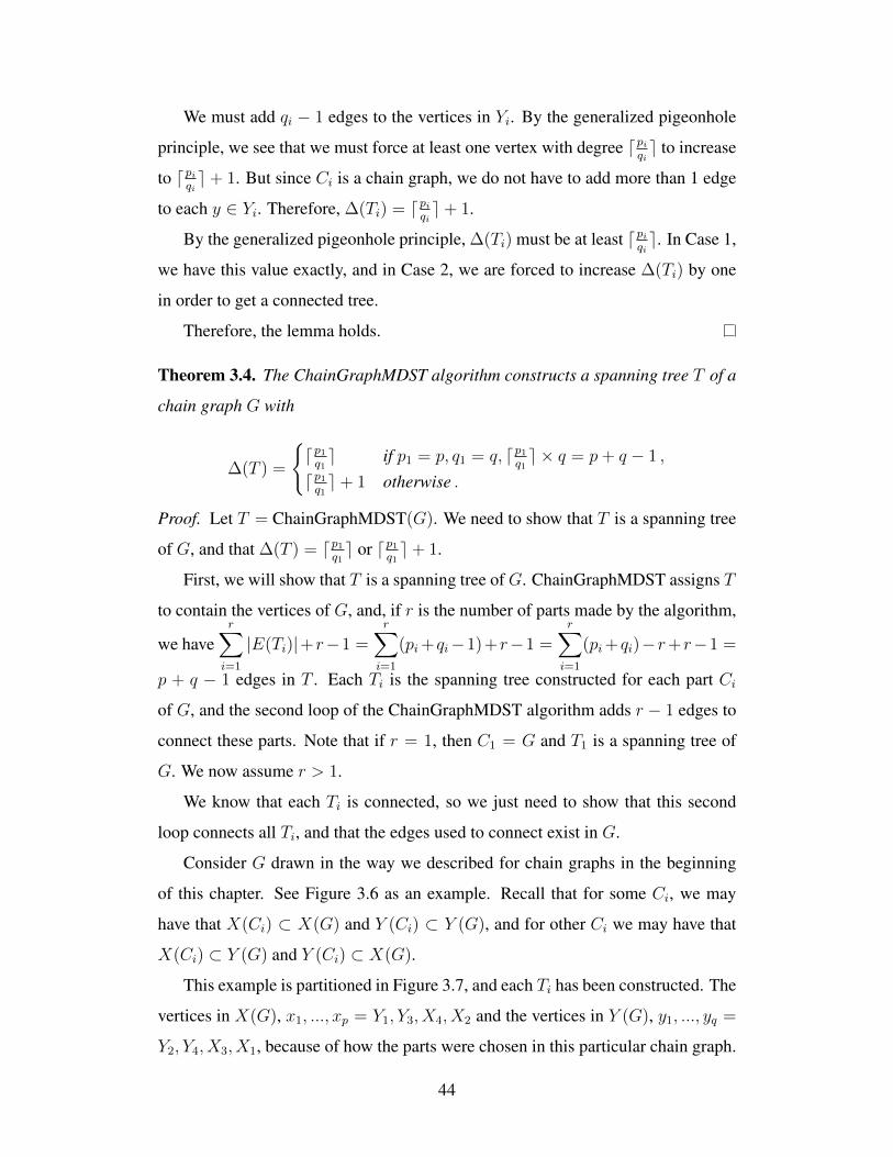
We must add qi − 1 edges to the vertices in Yi. By the generalized pigeonhole
principle, we see that we must force at least one vertex with degree dpiqie to increase
to dpiqie+ 1. But since Ci is a chain graph, we do not have to add more than 1 edge
to each y ∈ Yi. Therefore, ∆(Ti) = dpiqie+ 1.
By the generalized pigeonhole principle, ∆(Ti) must be at least dpiqie. In Case 1,
we have this value exactly, and in Case 2, we are forced to increase ∆(Ti) by one
in order to get a connected tree.
Therefore, the lemma holds.
Theorem 3.4. The ChainGraphMDST algorithm constructs a spanning tree T of a
chain graph G with
∆(T ) =
{dp1q1e if p1 = p, q1 = q, dp1
q1e × q = p+ q − 1 ,
dp1q1e+ 1 otherwise .
Proof. Let T = ChainGraphMDST(G). We need to show that T is a spanning tree
of G, and that ∆(T ) = dp1q1e or dp1
q1e+ 1.
First, we will show that T is a spanning tree of G. ChainGraphMDST assigns T
to contain the vertices of G, and, if r is the number of parts made by the algorithm,
we haver∑i=1
|E(Ti)|+r−1 =r∑i=1
(pi+qi−1)+r−1 =r∑i=1
(pi+qi)−r+r−1 =
p + q − 1 edges in T . Each Ti is the spanning tree constructed for each part Ci
of G, and the second loop of the ChainGraphMDST algorithm adds r − 1 edges to
connect these parts. Note that if r = 1, then C1 = G and T1 is a spanning tree of
G. We now assume r > 1.
We know that each Ti is connected, so we just need to show that this second
loop connects all Ti, and that the edges used to connect exist in G.
Consider G drawn in the way we described for chain graphs in the beginning
of this chapter. See Figure 3.6 as an example. Recall that for some Ci, we may
have that X(Ci) ⊂ X(G) and Y (Ci) ⊂ Y (G), and for other Ci we may have that
X(Ci) ⊂ Y (G) and Y (Ci) ⊂ X(G).
This example is partitioned in Figure 3.7, and each Ti has been constructed. The
vertices in X(G), x1, ..., xp = Y1, Y3, X4, X2 and the vertices in Y (G), y1, ..., yq =
Y2, Y4, X3, X1, because of how the parts were chosen in this particular chain graph.
44
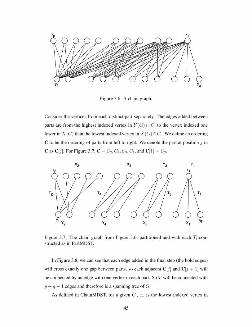
Figure 3.6: A chain graph.
Consider the vertices from each distinct part separately. The edges added between
parts are from the highest indexed vertex in Y (G) ∩ Ci to the vertex indexed one
lower in X(G) than the lowest indexed vertex in X(G)∩Ci. We define an ordering
C to be the ordering of parts from left to right. We denote the part at position j in
C as C[j]. For Figure 3.7, C = C2, C4, C3, C1, and C[1] = C2.
Figure 3.7: The chain graph from Figure 3.6, partitioned and with each Ti con-structed as in PartMDST.
In Figure 3.8, we can see that each edge added in the final step (the bold edges)
will cross exactly one gap between parts, so each adjacent C[j] and C[j + 1] will
be connected by an edge with one vertex in each part. So T will be connected with
p+ q − 1 edges and therefore is a spanning tree of G.
As defined in ChainMDST, for a given Ci, xa is the lowest indexed vertex in
45
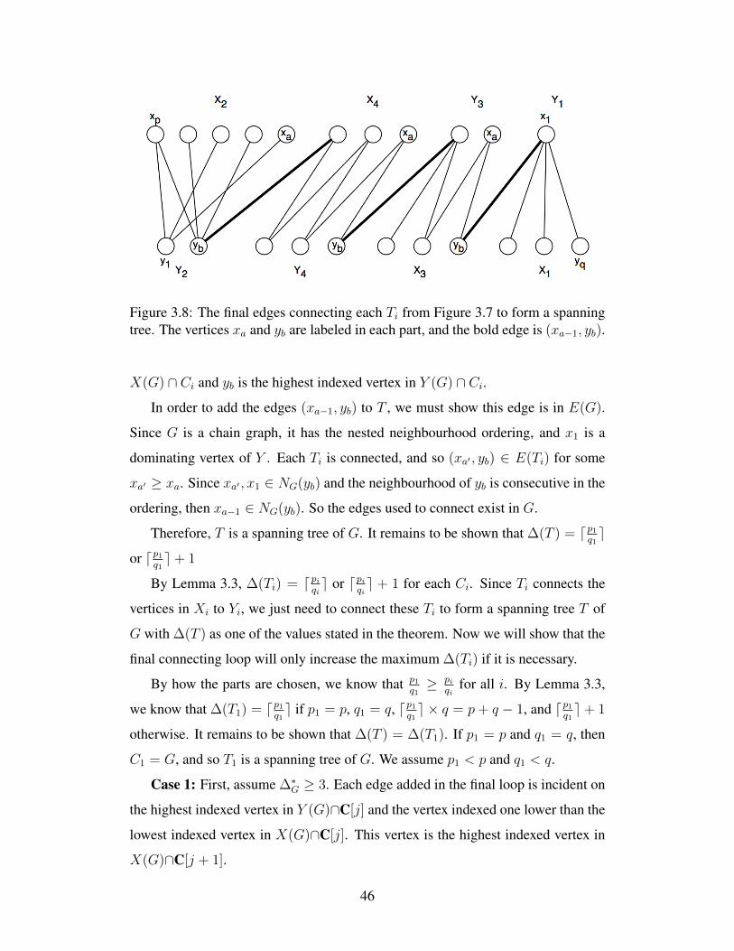
Figure 3.8: The final edges connecting each Ti from Figure 3.7 to form a spanningtree. The vertices xa and yb are labeled in each part, and the bold edge is (xa−1, yb).
X(G) ∩ Ci and yb is the highest indexed vertex in Y (G) ∩ Ci.
In order to add the edges (xa−1, yb) to T , we must show this edge is in E(G).
Since G is a chain graph, it has the nested neighbourhood ordering, and x1 is a
dominating vertex of Y . Each Ti is connected, and so (xa′ , yb) ∈ E(Ti) for some
xa′ ≥ xa. Since xa′ , x1 ∈ NG(yb) and the neighbourhood of yb is consecutive in the
ordering, then xa−1 ∈ NG(yb). So the edges used to connect exist in G.
Therefore, T is a spanning tree of G. It remains to be shown that ∆(T ) = dp1q1e
or dp1q1e+ 1
By Lemma 3.3, ∆(Ti) = dpiqie or dpi
qie + 1 for each Ci. Since Ti connects the
vertices in Xi to Yi, we just need to connect these Ti to form a spanning tree T of
G with ∆(T ) as one of the values stated in the theorem. Now we will show that the
final connecting loop will only increase the maximum ∆(Ti) if it is necessary.
By how the parts are chosen, we know that p1q1≥ pi
qifor all i. By Lemma 3.3,
we know that ∆(T1) = dp1q1e if p1 = p, q1 = q, dp1
q1e × q = p+ q − 1, and dp1
q1e+ 1
otherwise. It remains to be shown that ∆(T ) = ∆(T1). If p1 = p and q1 = q, then
C1 = G, and so T1 is a spanning tree of G. We assume p1 < p and q1 < q.
Case 1: First, assume ∆∗G ≥ 3. Each edge added in the final loop is incident on
the highest indexed vertex in Y (G)∩C[j] and the vertex indexed one lower than the
lowest indexed vertex in X(G)∩C[j]. This vertex is the highest indexed vertex in
X(G)∩C[j + 1].
46
We now consider two cases for xa−1 in C[j + 1]. Let Tl be the spanning tree
produced by PartMDST for C[j + 1]).
Subcase 1a: xa−1 ∈ X(C[j + 1])
As observed in the proof of Lemma 3.3, after PartMDST(C[j+1])), degTl(x) =
1 or 2, for all x ∈ X(Tl). So after this edge is added, degT (xa−1) = 2 or 3. Since
∆∗G ≥ 3, adding the edge (xa−1, yb) does not make degT (xa−1) > ∆(T1).
Subcase 1b: xa−1 ∈ Y (C[j + 1])
Let pj = |X(C[j+1])| and let qj = |Y (C[j+1])|. By Lemma 3.2, the maximum
degree of a vertex in Tl after the first loop in PartMDST is dpjqje. By Lemma 3.3,
the maximum degree of a vertex in Tl after PartMDST is dpjqje+ 1. However, since
only qj − 1 edges are added, at least one vertex in Y (C[j + 1]) has degree in Tl less
than ∆(Tl), or every vertex in Y (C[j + 1]) has the same degree.
In the first case, by Lemma 3.2, we know this is the highest indexed vertex in
Y (C[j + 1]). In this subcase, that vertex is xa−1, and so adding the edge (xa−1, yb)
does not make degT (xa−1) > ∆(T1). If all vertices in Y (C[j + 1]) have the same
degree, then a degree increase is required since, by how a part of chosen, X(C[j +
1]) has no neighbours in C[j], and therefore an edge connecting C[j] to C[j + 1]
must be have an edge incident on a vertex in Y (C[j + 1]).
Equivalent arguments can be made for the subcases that yb ∈ X(C[j]) and
yb ∈ Y (C[j]).
Case 2: Now assume ∆∗G = 2. This means thatG satisfies one of the conditions
from Theorem 3.1.
Subcase 2a: p = q and degG(xp) = degG(yp) = 1.
Partitioning G will give two parts, C1 and C2, with X1 = {xp, ..., x2} and
Y1 = {y1, ..., yp−1}, and X2 = {yp}, Y2 = {x1}.
PartMDST(C1) returns T1, which will be a path xp, y1, xp−1, y2, ..., x2, yp−1. T2
will contain only the edge (x1, yp). So the degree in T1 is 1 for xp, yp−1, x1, yp, and
2 for the other vertices. The algorithm will then add the edge (yp−1, x1), which will
not increase ∆(T ). Now ∆(T ) = ∆(T1) = 2, and T is a spanning tree of G.
Subcase 2b: p = q and at least one of degG(xq), degG(yp) > 1 OR p = q + 1.
G will be partitioned into just one part, C1. By Lemma 3.3, T1 is a spanning
47
tree of C1 with the ∆(T ) as defined in this theorem. C1 = G, so T1 = T and no
further edges are added.
Therefore, ChainGraphMDST returns a spanning tree T ofGwith ∆(T ) = dp1q1e
if p1 = p, q1 = q, dp1q1e × q = p+ q− 1, and dp1
q1e+ 1 otherwise. Thus, the theorem
holds.
3.3 Solving the Minimum Degree Spanning Tree Prob-lem on Chain Graphs
Theorem 3.5. Let G = (X, Y,E) be a chain graph with nested neighbourhood
ordering x1, ..., xp and y1, ..., yq. Recall the values k, l, ai, αi, bi, βi, as defined in
Section 3.2.1, as well as the ratios fX(i, G) and fY (i, G).
Fix c such that c ∈ {1, ..., k}, fX(c,G) ≥ fX(i, G) for 1 ≤ i < c, and
fX(c,G) > fX(i, G) for c < i ≤ k. Fix d such that d ∈ {1, ..., l}, fY (d,G) ≥
fY (i, G) for 1 ≤ i < d, and fY (d,G) > fY (i, G) for d < i ≤ l.
We now define a part C of G. If c ≥ d, let X(C) = {x ∈ X |degG(x) ≤ ac},
and Y (C) = NG(X(C)). If d > c, let X(C) = {y ∈ Y |degG(y) ≤ bd}, and
Y (C) = NG(X(C)). We note that X(C) and Y (C) may correspond to vertices in
Y (G) and X(G) respectively.
Let p1 and q1 be the sizes of X(C) and Y (C) respectively. Then,
∆∗G =
{dp1q1e if p1 = p, q1 = q, dp1
q1e × q = p+ q − 1 ,
dp1q1e+ 1 otherwise .
Proof. By Theorem 3.4, there exists a spanning tree T of a chain graph G such that
∆(T ) =
{dp1q1e if p1 = p, q1 = q, dp1
q1e × q = p+ q − 1 ,
dp1q1e+ 1 otherwise .
Therefore, ∆(G) ≤ ∆(T ).
We now show that, unless p = p1, q = q1 and dpqe×q = p+q−1, ∆∗G ≥ d
p1q1e+1.
We note that if p1 < p, then we must have q1 < q, otherwise the graph G− C1
is not connected.
48
If p > p1, and q > q1, then C1 is a proper subset of G. Connecting each vertex
in X1 to exactly one vertex in Y1 creates q1 components. We must now add q1 − 1
edges to connect these components, plus one edge to connect this part to the rest of
the graph. Therefore, there are p1 + q1 edges incident on Y1, and by the generalized
pigeonhole principle, at least one vertex in Y1 has degree ≥ dp1+q1q1e = dp1
q1e + 1.
Thus in this case, ∆∗G ≥ dp1q1e+ 1.
If p = p1 and q = q1, then we must add p + q − 1 edges to the vertices in Y
to create a spanning tree. Connecting the vertices in X to the vertices in Y gives
at least one vertex in Y with degree ≥ dpqe. If there is exactly one vertex in Y
with degree ≥ dpqe after connecting the vertices in X , then adding the remaining
q − 1 edges can be done without increasing the degree. This case only occurs if
dpqe × q = p + q − 1. Otherwise, two or more vertices have degree ≥ dp
qe after
connecting the vertices of X , and adding q − 1 more edges will give at least one
vertex with degree ≥ dpqe+ 1. Thus, unless dp
qe × q = p+ q − 1, ∆∗G ≥ d
p1q1e+ 1.
Therefore, this formula gives ∆∗G for any chain graph G.
Theorem 3.6. The ChainGraphMDST algorithm produces an MDST of a given
chain graph G in O(n2) time.
Proof. By Theorem 3.4, ChainGraphMDST produces a spanning tree T of G such
that
∆(T ) =
{dp1q1e if p1 = p, q1 = q, dp1
q1e × q = p+ q − 1 ,
dp1q1e+ 1 otherwise .
By Theorem 3.5,
∆∗G =
{dp1q1e if p1 = p, q1 = q, dp1
q1e × q = p+ q − 1 ,
dp1q1e+ 1 otherwise .
Therefore, ChainGraphMDST produces a spanning tree T ofG such that ∆(T ) =
∆∗G.
The algorithm Partition calls ComputeRatios, which checks the ratios for G′,
which in the worst case has k = p and l = q, and so ComputeRatios runs in
O(|G′|) ∈ O(n) time. Partition then adds some number of vertices to the new part,
which isO(n), and thus Partition runs inO(n) time. The PartMDST algorithm adds
one edge for each vertex in Ci, and so runs in O(n) time.
49
The ChainGraphMDST algorithm calls Partition and PartMDST once for each
part in the partition of G. The upper bound on the number of parts r is q, since at
least one vertex from each of X and Y must be in a part. Thus, in the worst case,
the first loop of ChainGraphMDST runs in q ∗ (O(n) + O(n)) ∈ O(n2) time. The
second loop of ChainGraphMDST runs in O(r) time.
Therefore, the ChainGraphMDST algorithm runs in O(n2) time.
50
Chapter 4
Bipartite Permutation Graphs
We present results related to the minimum degree spanning tree problem for bi-
partite permutation graphs. First, we give some structural results regarding longest
paths in bipartite permutation graphs. We then show that there exists a crossing-
free MDST for every connected bipartite permutation graph, and one that contains
a longest path.
We combine these to show that for every connected bipartite permutation graph
G, there exists a spanning tree T of G such that T is a caterpillar, T contains a
longest path of G, T has no edge crossings, and ∆(T ) = ∆∗G.
Finally, we present a polynomial time algorithm that uses dynamic program-
ming to solve the minimum degree spanning tree problem and the minimum degree
spanning tree construction problem on connected bipartite permutation graphs.
Let G = (X, Y,E) be a bipartite permutation graph with strong ordering
x1, ..., xp and y1, ...yq. We will consider G drawn with the vertices of X and Y
in rows, sorted as in a strong ordering, as in Figure 4.1. We consider a vertex xi to
be to the left of a vertex xj , xi, xj ∈ X , if i < j, and to the right if i > j. The same
holds for yi, yj ∈ Y .
We define some order on a set of edge crossings in a strongly ordered bipartite
permutation graph. Consider a set of edges F such that every edge in the set forms a
crossing with at least one other edge. Let xi1 , xi2 , ..., xik and yj1 , yj2 , ..., yjh , ordered
as in the strong ordering, be the vertices contained in the edges in F . We define the
leftmost edge crossing as the pair of edges (xi1 , y′) and (x′, yj1), where y′ is the
leftmost neighbour in F of xi1 and x′ is the leftmost neighbour in F of yj1 . This
51
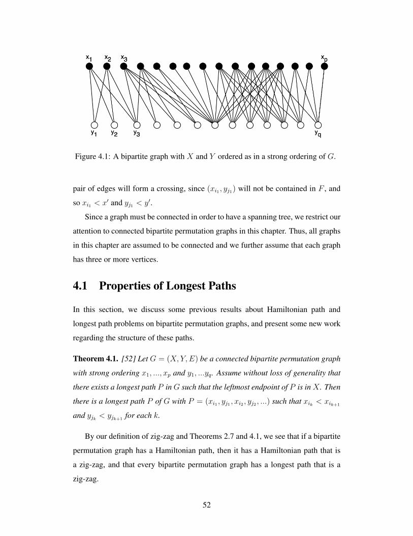
Figure 4.1: A bipartite graph with X and Y ordered as in a strong ordering of G.
pair of edges will form a crossing, since (xi1 , yj1) will not be contained in F , and
so xi1 < x′ and yj1 < y′.
Since a graph must be connected in order to have a spanning tree, we restrict our
attention to connected bipartite permutation graphs in this chapter. Thus, all graphs
in this chapter are assumed to be connected and we further assume that each graph
has three or more vertices.
4.1 Properties of Longest Paths
In this section, we discuss some previous results about Hamiltonian path and
longest path problems on bipartite permutation graphs, and present some new work
regarding the structure of these paths.
Theorem 4.1. [52] Let G = (X, Y,E) be a connected bipartite permutation graph
with strong ordering x1, ..., xp and y1, ...yq. Assume without loss of generality that
there exists a longest path P inG such that the leftmost endpoint of P is inX . Then
there is a longest path P of G with P = (xi1 , yj1 , xi2 , yj2 , ...) such that xik < xik+1
and yjk < yjk+1for each k.
By our definition of zig-zag and Theorems 2.7 and 4.1, we see that if a bipartite
permutation graph has a Hamiltonian path, then it has a Hamiltonian path that is
a zig-zag, and that every bipartite permutation graph has a longest path that is a
zig-zag.
52
We now present some results regarding the edges (x1, y1) and (xp, yq) in longest
paths of G.
Theorem 4.2. [1] Let G = (X, Y,E) be a biconvex graph with convex orderings
x1, ..., xp and y1, ..., y1. Then G is a bipartite permutation graph if and only if
(x1, y1), (xp, yq) ∈ E.
Lemma 4.3. Let G = (X, Y,E) be a connected bipartite permutation graph with
strong ordering x1, ..., xp and y1, ..., y1. Then at least one of x1, y1 is in every zig-
zag longest path in G.
Proof. Assume there exists a longest zig-zag path P in G such that neither x1 or
y1 are in P . Assume without loss of generality P = (xi, yj, ...), i > 1, j > 1. We
have stated that we are only dealing with connected graphs, so there exists a path
in G from xi to x1. If there exists a path in G from xi to x1 that contains (xi, yk),
yk /∈ P , then P is not a longest path in G, as it could be extended by adding the
edges in the (xi, x1)-path. So yj is on the (xi, x1)-path in G. If this path is longer
than length 1, replacing (xi, yj) with this path would give a path inG longer than P .
So (x1, yj) ∈ E. But replacing (xi, yj) with (x1, yj), (x1, y1) gives a longer zig-zag
path.
Therefore, any zig-zag longest path in G must contain at least one of x1, y1.
Lemma 4.4. Let G = (X, Y,E) be a connected bipartite permutation graph with
strong ordering x1, ..., xp and y1, ..., y1. Then there exists a zig-zag longest path P
in G such that (x1, y1) ∈ P .
Proof. By Lemma 4.3, at least one of x1, y1 is in every zig-zag longest path of G.
Assume for all zig-zag longest paths of G, we have exactly one of x1, y1 in each
path. By Theorem 4.2, we have (x1, y1) ∈ E.
Let P be an arbitrary zig-zag longest path of G. Assume without loss of gen-
erality that x1 ∈ V (P ) and y1 /∈ V (P ). Since P is a longest path, x1 must have
degree two in P , otherwise we could add (x1, y1) to P to extend the path. So
P = (yj, x1, ...) for some yj .
53
Let P ′ = (V (P ) − {yj} ∪ {y1}, E(P ) − {(x1, yj)} ∪ {(x1, y1)}). But P ′ is a
zig-zag longest path in G. So there exists a longest path in G that contains the edge
(x1, y1).
The proof of this lemma also shows that a path that does not contain (x1, y1)
can be used to construct a path that contains this edge.
Corollary 4.5. LetG = (X, Y,E) be a connected bipartite permutation graph with
strong ordering x1, ..., xp and y1, ..., y1. Let P be a zig-zag longest path in G with
its leftmost endpoint in one side of the graph (either X or Y ) that does not contain
the edge (x1, y1). Then there exists a zig-zag longest path in G, P ′, that has its
leftmost endpoint in the same side of the graph as P , contains the edge (x1, y1),
and is equivalent to P in positions 2, ..., r.
Let P = v1, v2, ..., vk be a zig-zag longest path of a strongly ordered connected
bipartite permutation graph G. P is a leftmost longest path if for each vi, there does
not exist a longest path P ′ such that the vertex at index i in P ′ is lower indexed than
vi. A bipartite permutation graph has either one or two leftmost longest paths. If it
has two, one has its leftmost endpoint in X and the other has its leftmost endpoint
in Y .
Lemma 4.6. Let G = (X, Y,E) be a connected bipartite permutation graph with
strong ordering x1, x2, ..., xp, y1, y2, ..., yq, and let P be a leftmost longest path in
G. Then P contains the edge (x1, y1).
Proof. Let P be a leftmost longest path inG that does not contain the edge (x1, y1),
and assume without loss of generality that the leftmost endpoint of P is in X .
Therefore, P contains some edge (xi, y1) such that i > 1. So P = (xi, y1, ...).
By Lemma 4.4, there exists some zig-zag longest path P ′ that contains (x1, y1).
So P ′ = (x1, y1, ...). By the definition of leftmost longest path, we get a contradic-
tion.
Therefore, (x1, y1) is in every leftmost longest path of G.
54
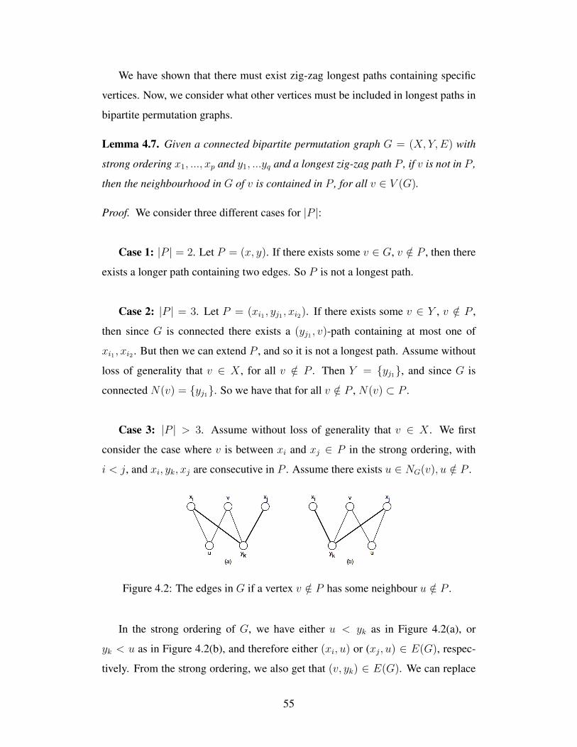
We have shown that there must exist zig-zag longest paths containing specific
vertices. Now, we consider what other vertices must be included in longest paths in
bipartite permutation graphs.
Lemma 4.7. Given a connected bipartite permutation graph G = (X, Y,E) with
strong ordering x1, ..., xp and y1, ...yq and a longest zig-zag path P , if v is not in P ,
then the neighbourhood in G of v is contained in P , for all v ∈ V (G).
Proof. We consider three different cases for |P |:
Case 1: |P | = 2. Let P = (x, y). If there exists some v ∈ G, v /∈ P , then there
exists a longer path containing two edges. So P is not a longest path.
Case 2: |P | = 3. Let P = (xi1 , yj1 , xi2). If there exists some v ∈ Y , v /∈ P ,
then since G is connected there exists a (yj1 , v)-path containing at most one of
xi1 , xi2 . But then we can extend P , and so it is not a longest path. Assume without
loss of generality that v ∈ X , for all v /∈ P . Then Y = {yj1}, and since G is
connected N(v) = {yj1}. So we have that for all v /∈ P , N(v) ⊂ P .
Case 3: |P | > 3. Assume without loss of generality that v ∈ X . We first
consider the case where v is between xi and xj ∈ P in the strong ordering, with
i < j, and xi, yk, xj are consecutive in P . Assume there exists u ∈ NG(v), u /∈ P .
Figure 4.2: The edges in G if a vertex v /∈ P has some neighbour u /∈ P .
In the strong ordering of G, we have either u < yk as in Figure 4.2(a), or
yk < u as in Figure 4.2(b), and therefore either (xi, u) or (xj, u) ∈ E(G), respec-
tively. From the strong ordering, we also get that (v, yk) ∈ E(G). We can replace
55
(xi, yk, xj) ∈ P with either (xi, u, v, yk, xj) or (xi, yk, v, u, xj). But P is a longest
path. Therefore NG(v) ⊂ P .
Now consider the case that v is not between two path vertices in the strong
ordering. We will say that v is on an end of G; that is for XP being the set of
vertices in X that are in P , we have v < w, for all w ∈ XP , or v > w, for
all w ∈ XP . Consider the set of vertices U = {u|u ∈ NG(v), u /∈ P and u is
not between two path vertices in the strong ordering}. U is also on an end of G,
and therefore the vertices of U are consecutive in the strong ordering of G. The
subgraph of G induced by {v} ∪ U ∪ {p}, where p ∈ P with degP (p) = 1 and the
distance in G between v and p is minimized, is a bipartite permutation graph where
both X and Y are non-empty and no vertices other than p are in P . Since v and U
are on the ends of G, there exists a path from v to p that contains no vertices in P
other than p. Adding this path to P gives us a longer path. But P is a longest path,
so v cannot have such a subset U in its neighbourhood.
Therefore, for any vertex v /∈ P , we have that NG(v) ⊂ P .
Lemma 4.8. Let G = (X, Y,E) be a connected, strongly ordered bipartite permu-
tation graph. For all v ∈ G, if degG(v) ≥ 2, then v is on some longest path in
G.
Proof. Let P be an arbitrary longest zig-zag path of G. Let v be a vertex with
degG(v) ≥ 2 that is not in V (P ). Assume without loss of generality that v ∈ X .
From Lemma 4.7, we have that NG(v) ⊂ V (P ). Choose two neighbours of v,
ui, uj such that ui, uj ∈ P , ui, uj ∈ Y , and no vertex of P is between them in the
strong ordering of Y . By the adjacency property of bipartite permutation graphs,
we have two vertices that satisfy this requirement. Therefore in P we have ui, w, uj
consecutively for some w ∈ X . By replacing w in P by v gives another longest
path.
Therefore, any vertex v with degG(v) ≥ 2 is on some longest path of G.
We now show that the existence of certain zig-zag longest paths in a bipartite
56
permutation graph give more information about the graph. More specifically, if a
bipartite permutation graph G has zig-zag longest paths beginning in both X and
Y , this tells us the value of ∆∗G.
Let P be a zig-zag longest path of a strongly ordered connected bipartite per-
mutation graph G. Let r be the size of a longest path in G, and P = v1, v2, ..., vr.
We refer to the index i of vi ∈ P as the position of vi in P . Let the leftmost endpoint
of P be v1 and the rightmost endpoint of P be vr.
In the remainder of this section, we consider G = (X, Y,E), a strongly ordered
bipartite permutation graph that has zig-zag longest paths with leftmost endpoints
in both X and Y . Let PX and PY be zig-zag longest paths of G, PX with leftmost
endpoint inX and PY with leftmost endpoint in Y . By Lemma 4.4, we can fix these
paths to both contain the edge (x1, y1). Assume both paths contain this edge, which
means that the leftmost endpoint of PX is x1, and the leftmost endpoint of PY is y1.
We now introduce some definitions related to PX and PY . Let pos(v, P ) be the
position in zig-zag path P of vertex v. The leftmost endpoint has position 1, etc. A
vertex v ∈ PX ∪ PY satisfies the Position Condition if one of the following holds:
• v ∈ X(PX ∩ PY ) and pos(v, PX) < pos(v, PY ), or• v ∈ Y (PX ∩ PY ) and pos(v, PY ) < pos(v, PX), or• v /∈ PX ∩ PY
We define front(P, v) to be the set of vertices in a zig-zag path P that have po-
sition less than pos(v, P ) and back(P, v) to be the set of vertices in P that have po-
sition greater than pos(v, P ). A vertex u is to the left of v ∈ P if u ∈ front(P, v).
A vertex u is to the right of v ∈ P if u ∈ back(P, v). For a vertex w /∈ P , consider
the subpath u1, v, u2 in P such that u1 < w < u2 in the strong ordering of the
original bipartite permutation graph. We define vertices to the left and right of w to
be those to the left and right of v.
Lemma 4.9. Let xi1 , yj1xi2 , yj2 be a subpath of PX such that the Position Condition
holds for these vertices and all vertices to their left in PX . Then (xi1 , yj2) ∈ E(G).
Proof. Assume that for all four vertex subpaths of PX beginning in X to the left of
xi1 , yj1 , xi2 , yj2 , there exists an edge in G between the first and fourth vertices in the
57
subpath. Therefore, xi1 , yj1 , xi2 , yj2 is the leftmost such subpath of PX where we
don’t know if this edge exists.
By Lemma 4.7, at least one of xi1 , yj1 is in PY . We consider the following cases.
Case 1: Assume xi1 , yj1 ∈ PY . Let y′ be the rightmost neighbour of xi1 in
PY . If y′ ≥ yj2 , then by the adjacency property, (xi1 , yj2) ∈ G. Therefore, assume
y′ < yj2 .
If y′ ≤ yj1 , let a = pos(xi1 , PX) and b = pos(xi1 , PY ). By our assumption,
a < b. We have pos(y′, PY ) = b+ 1 and pos(yj1 , PX) = a+ 1. Because y′ is to the
left of yj1 in PY and the Position Condition holds for yj1 , we have that b+1 ≤ a+1
implies b ≤ a, a contradiction.
Now assume yj1 < y′ < yj2 . Since PX is a zig-zag, we know y′ /∈ PX . We
now show we can build a longer path containing y′ and the vertices of PX to get a
contradiction.
If xi1 , yj1 = x1, y1, let P ′ = y1, x1, y′, xi2 , yj2 , α, where α is the rest of PX
following yj2 . P ′ is longer than PX , but PX is a longest path and so we have a
contradiction.
Otherwise, let P ′ = PX , and then for each four-vertex subpath xi3 , yj3 , xi4 , yj4 in
P ′ to the left of xi1 , remove the edge (xi4 , yj3) and add the edge (xi3 , yj4). Remove
(xi2 , yj1) and add (xi1 , y′), (xi2 , y
′). Now P ′ is a longer path than PX and we get a
contradiction.
Case 2: Assume xi1 ∈ PY and yj1 /∈ PY . Let y′ be the rightmost neighbour of
xi1 in PY . If y′ ≥ yj2 , then by the adjacency property, (xi1 , yj2) ∈ G.
If y′ < yj1 , we can use the fact that the Position Condition holds for xi1
to get a longer path. We see that |front(PY , xi1)| > |front(PX , xi1)|, and so
|back(PX , xi1)| > |back(PY , xi1)|. Since y′ < yj1 , and PX and PY are zig-zags, we
have that front(PY , xi1) ∩ back(PX , xi1) = ∅. Therefore, we can obtain a longer
path P ′ = front(PY , xi1) ∪ {xi1} ∪ back(PX , xi1), a contradiction.
Now, assume yj1 < y′ < yj2 . We know y′ /∈ PX and so we can construct a
longer path containing y′ and the vertices of PX as in Case 1.
Case 3: Assume xi1 /∈ PY and yj1 ∈ PY . Let x′ be the rightmost neighbour of
yj1 in PY .
58
Subcase 3.a: Assume x′ < xi1 and let y′ be the rightmost neighbour of x′
in PY . If y′ ≥ yj2 , then by the adjacency property, (xi1 , yj2) ∈ G. Otherwise,
yj1 < y′ < yj2 and y′ /∈ PX , and we can construct a longer path P ′ that contains y′
and the vertices of PX as in Case 1.
Subcase 3.b: If x′ > xi2 and xi2 /∈ PY , by Lemma 4.7, we know that we must
have yj2 ∈ PY . We have that front(PX , yj2) ∩ back(PY , yj2) = ∅, and because the
Position Condition holds for yj2 , we can build a longer path P ′ = front(PX , yj2)∪
{yj2} ∪ back(PY , yj2), a contradiction.
Subcase 3.c: If x′ > xi2 and xi2 ∈ PY , let a = pos(yj1 , PX) and b =
pos(yj1 , PY ), and so b < a because the Position Condition holds for yj1 . Now
pos(xi2 , PY ) ≤ b − 1 and pos(xi2 , PX) = a + 1. Because the Position Condition
holds for xi2 , we have a+1 < b−1, which gives us a+2 < b, and so a+2 < b < a,
a contradiction.
Subcase 3.d: Assume x′ = xi2 . By the Position Condition, we have pos(yj1 , PY )
< pos(yj1 , PX). The edge (xi2 , yj1) is in both PX and PY , so we get pos(xi2 , PY ) =
pos(yj1 , PY ) + 1 and pos(xi2 , PX) = pos(yj1 , PX) + 1. This means pos(xi2 , PY ) <
pos(xi2 , PX), which contradicts our assumption that the Position Condition holds
for xi2 .
Subcase 3.e: Assume xi1 < x′ < xi2 . If the rightmost neighbour y′ of x′ in PY is
to the left of yj2 , then y′ /∈ PX and we can construct a longer path P ′ that contains y′
and the vertices of PX as in Case 1. Otherwise, by our assumptions in this case, and
because PX and PY are zig-zags, we have that front(PX , yj1)∩ back(PY , yj1) = ∅,
and because the Position Condition holds for yj1 , we can build a longer path P ′ =
front(PX , yj1) ∪ {yj1} ∪ back(PY , yj1), a contradiction.
Therefore, if the Position Condition holds for a subpath xi1 , yj1 , xi2 , yj2 in PX
and all vertices to the left of this subpath, then (xi1 , yj2) ∈ G.
Corollary 4.10. Consider PX as defined above in a bipartite permutation graph
G. If there exists a vertex y ∈ Y (G) with y /∈ PX , and if the Position Condition is
satisfied for all vertices in PX that are to the left of y, then there exists a path that
is longer than PX . Therefore, when the Position Condition holds in PX , there are
59
no vertices in Y (G) − Y (PX). Equivalently, when the Position Condition holds in
PY , there are no vertices in X(G)−X(PY ).
Proof. The proof of Lemma 4.9, Case 1 shows how if such a vertex in Y (G) −
Y (PX) exists, we can construct a path that is longer than PX .
Corollary 4.11. Using an equivalent argument as in the proof of Lemma 4.9, we can
show that for any subpath yj1 , xi1 , yj2 , xi2 ∈ PY such that the Position Condition
holds for these vertices and all vertices to their left in PY , then (yj1 , xi2) ∈ G.
Lemma 4.12. The Position Condition holds for all vertices in PX ∪ PY .
Proof. First, since PX starts in X and alternates between X and Y along its length,
and PY starts in Y , we can never have a vertex occupying the same position in both
paths. In PX , all odd vertices are in X and all even vertices are in Y . The reverse is
true for PY . This means we don’t have to worry about equality.
PX begins with x1 then y1, and PY begins with y1, then x1. We can see the
lemma holds here.
Assume that the Position Condition holds in PX up to some vertex. We first
assume this vertex is x′ ∈ X(PX), and then that it is y′ ∈ Y (PX).
Let x′ ∈ X be the leftmost vertex in PX where the Position Condition does
not hold. Then we must have x′ ∈ PX ∩ PY and pos(x′, PX) > pos(x′, PY ). If
front(PX , x′)∩ back(PY , x
′) = ∅, then we can get a longer path P ′ = front(PX , x′)
∪ {x′} ∪ back(PY , x′).
Assume front(PX , x′) ∩ back(PY , x′) 6= ∅. Let this non-empty set be Q. Let
y′′ be the rightmost neighbour of x′ in PY . Since Q is non-empty, y′′ must be to the
left of the rightmost neighbour of x′ in PX .
Case 1: Assume y′′ ∈ NPX(x′). Here we have two options: y′′ can be the left
neighbour of x′ in PX or it can be the right neighbour. First, assume y′′ is the left
neighbour of x′ in PX . By our assumptions, the Position Condition holds for y′′.
That is, pos(y′′, PY ) < pos(y′′, PX). Because PX and PY share the edge (x′, y′′),
we have that front(PX , y′′) ∩ back(PY , y′′) = ∅. Therefore, we can build P ′ =
front(PX , y′′) ∪ {y′′} ∪ back(PY , y
′′), which is a longer path, a contradiction.
60
Now assume y′′ is the right neighbour of x′ in PX . Then the edge (x′, y′′) is in
both PX and PY and in both cases, y′′ is the rightmost neighbour of x′. Since these
paths are zig-zags, this shows that front(PX , x′) ∩ back(PY , x′) = ∅, a contradic-
tion.
Case 2: Assume y′′ is to the left of the leftmost neighbour of x′ in PX and
y′′ ∈ PX . By our assumptions, the Position Condition holds for y′′, so pos(y′′, PY )
< pos(y′′, PX). The rightmost neighbour of y′′ in PY is to the right of x′, so
front(PX , y′′) ∩ back(PY , y
′′) = ∅, and so we can build a longer path P ′ =
front(PX , y′′) ∪ {y′′} ∪ back(PY , y
′′), a contradiction.
Case 3: Assume y′′ /∈ PX and y′′ is between the two neighbours of x′ in PX or
y′′ is to the left of the leftmost neighbour of x′ in PX . Let xi1 , yj1 , xi2 be the subpath
of PX such that yj1 is the nearest vertex in PX to the left of y′′. By Lemma 4.9, for
each four vertex subpath of PX starting in X to the left of x′, the edge between the
first and fourth vertices is in G. Let P ′ = PX . For each four vertex subpath of P ′
starting in X such that all vertices in the subpath are to the left of xi2 , remove the
edge connecting the second and third vertices and add an edge connecting the first
and fourth. Remove (xi2 , yj1) and add (xi1 , y′′), (xi2 , y
′′). Now P ′ is a longer path
in G containing y′′ and the vertices of PX , a contradiction.
These cases prove that all vertices in X(PX) must satisfy the Position Condi-
tion.
Now, let y′ ∈ Y be the leftmost vertex in PX where the Position Condition does
not hold. Let a = pos(y′, PY ) and let b = pos(y′, PX). We have a > b. Since PX
and PY are paths in a bipartite graph that start in X and Y respectively, then a is
odd and b is even. The number of vertices in Y in the (y1, y′)-subpath of PY is da
2e.
The number of vertices in Y in the (x1, y′)-subpath of PX is b
2.
Since a is odd, b is even, and a > b, then da2e > b
2. Therefore, there exists
some y ∈ PY such that y /∈ PX and y1 < y < y′. Let xi1 , yj1 , xi2 be the subpath
of PX such that yj1 is the nearest vertex in PX to the left of y. By Lemma 4.9, for
each four vertex subpath of PX starting in X to the left of y′, the edge between the
first and fourth vertices is in G. Let P ′ = PX . For each four vertex subpath of P ′
starting in X such that all vertices in the subpath are to the left of xi2 , remove the
61
edge connection the second and third vertices and add an edge connecting the first
and fourth. Remove (xi2 , yj1) and add (xi1 , y), (xi2 , y). Now P ′ is a longer path in
G containing y′′ and the vertices of PX , a contradiction.
In each case we get a contradiction to our initial assumption that there exists a
vertex in PX where the Position Condition does not hold. Therefore, the Position
Condition holds for every vertex in PX . We can make a symmetrical argument for
PY , and so therefore the Position Condition holds for all vertices in PX ∪ PY .
Corollary 4.13. PX contains all vertices in Y (G) and PY contains all vertices in
X(G).
Proof. By Corollary 4.10, when the Position Condition holds PX skips no vertices
in Y and PY skips no vertices in X . Then by Lemma 4.12, we get that V (PX) ⊃
Y (G) and V (PY ) ⊃ X(G).
Lemma 4.14. If a strongly ordered, connected bipartite permutation graph G =
(X, Y,E) has at least one zig-zag longest path that starts in X and another zig-zag
longest path that starts in Y , then G has exactly these two zig-zag longest paths,
and they contain exactly the same vertices. More specifically, if PX = v1, v2, ...,
vr−1, vr, then PY = v2, v1, ..., vr, vr−1. That is, for each ordered pair of vertices
vi, vi+1 in PX with i odd, then vi+1, vi is an ordered pair in PY .
Proof. First, we show that r is even, and so PX has its rightmost endpoint in Y , and
PY in X .
Assume that r is odd. Since G is bipartite, we have |X(PX)| = |Y (PX)|+ 1 =
|X(PY )|+ 1 = |Y (PY )|. Then there exists some x in X(PX) such that x /∈ PY .
By Corollary 4.13, X(G) ⊂ V (PY ).
Therefore, r must be even.
Assume that PX and PY contain the same alternating vertices up to xi1 , yj1 , and
after these vertices is the first place they differ. Let PX = x1, y1, ..., xi1 , yj1 , xi2 ,
yj2 , ... and PY = y1, x1, ..., yj1 , xi1 , yj3 , xi3 , .... Now we want to show that xi2 = xi3
and yj2 = yj3 .
First, consider yj3 . By Corollary 4.13, yj3 ∈ PX . Assume yj3 6= yj2 . Since PX
is a zig-zag, then yj2 < yj3 . Since PY is a zig-zag, this means yj2 /∈ PY . Since r
62
is even, if there is some vertex in Y (PX − PY ), then there is also some vertex in
Y (PY − PX). But this contradicts Corollary 4.13 as PX cannot skip any vertices in
Y (G), and so we must have that yj2 = yj3 .
Now consider xi3 . Assume xi2 6= xi3 . By Corollary 4.13, xi2 ∈ PY . Since PY
is a zig-zag, then xi3 < xi2 . Since PX is a zig-zag, this means xi3 /∈ PX . Since r
is even, if there is some vertex in X(PY − PX), then there is also some vertex in
X(PX −PY ). But this contradicts Corollary 4.13 as PY cannot skip any vertices in
X(G). Therefore, we must have that xi2 = xi3 .
We assumed that PX and PY differed after xi1 , yj1 . Therefore, the lemma holds
by contradiction.
Corollary 4.15. If G has PX and PY , then G has no other zig-zag longest paths
and ∆∗G = 2.
Proof. By Corollary 4.13, the symmetry of the strong ordering of bipartite permu-
tation graphs, and because we have shown that PX has its rightmost endpoint in Y
and PY has its rightmost endpoint in X , we have that PX and PY can not skip any
vertex in either X(G) or Y (G). Therefore, they are both Hamiltonian paths.
4.2 Crossing-Free Minimum Degree Spanning Trees
In the previous section, we looked at longest paths in bipartite permutation graphs
that contain no edge crossings. Now, we consider crossing-free spanning trees and
MDSTs in bipartite permutation graphs.
Theorem 4.16. [20] A bipartite graph with a vertex ordering x1, ..., xp, y1, ..., yq
contains no edge crossings only if each connected component is a caterpillar.
Lemma 4.17. Let G = (X, Y,E) be a connected bipartite permutation graph with
strong ordering x1, ..., xp and y1, ..., y1. Then any spanning tree of G with no edge
crossings contains the edges (x1, y1) and (xp, yq).
Proof. Assume the edge (x1, y1) is not in a crossing-free spanning tree of G. Then
x1 must be adjacent to some vertex y′ such that y′ > y1, and y1 must be adjacent to
63
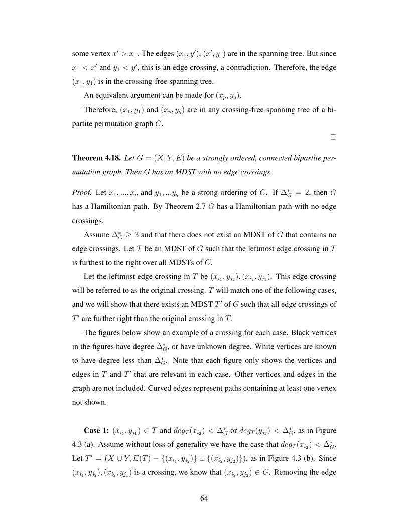
some vertex x′ > x1. The edges (x1, y′), (x′, y1) are in the spanning tree. But since
x1 < x′ and y1 < y′, this is an edge crossing, a contradiction. Therefore, the edge
(x1, y1) is in the crossing-free spanning tree.
An equivalent argument can be made for (xp, yq).
Therefore, (x1, y1) and (xp, yq) are in any crossing-free spanning tree of a bi-
partite permutation graph G.
Theorem 4.18. Let G = (X, Y,E) be a strongly ordered, connected bipartite per-
mutation graph. Then G has an MDST with no edge crossings.
Proof. Let x1, ..., xp and y1, ...yq be a strong ordering of G. If ∆∗G = 2, then G
has a Hamiltonian path. By Theorem 2.7 G has a Hamiltonian path with no edge
crossings.
Assume ∆∗G ≥ 3 and that there does not exist an MDST of G that contains no
edge crossings. Let T be an MDST of G such that the leftmost edge crossing in T
is furthest to the right over all MDSTs of G.
Let the leftmost edge crossing in T be (xi1 , yj2), (xi2 , yj1). This edge crossing
will be referred to as the original crossing. T will match one of the following cases,
and we will show that there exists an MDST T ′ of G such that all edge crossings of
T ′ are further right than the original crossing in T .
The figures below show an example of a crossing for each case. Black vertices
in the figures have degree ∆∗G, or have unknown degree. White vertices are known
to have degree less than ∆∗G. Note that each figure only shows the vertices and
edges in T and T ′ that are relevant in each case. Other vertices and edges in the
graph are not included. Curved edges represent paths containing at least one vertex
not shown.
Case 1: (xi1 , yj1) ∈ T and degT (xi2) < ∆∗G or degT (yj2) < ∆∗G, as in Figure
4.3 (a). Assume without loss of generality we have the case that degT (xi2) < ∆∗G.
Let T ′ = (X ∪ Y,E(T ) − {(xi1 , yj2)} ∪ {(xi2 , yj2)}), as in Figure 4.3 (b). Since
(xi1 , yj2), (xi2 , yj1) is a crossing, we know that (xi2 , yj2) ∈ G. Removing the edge
64
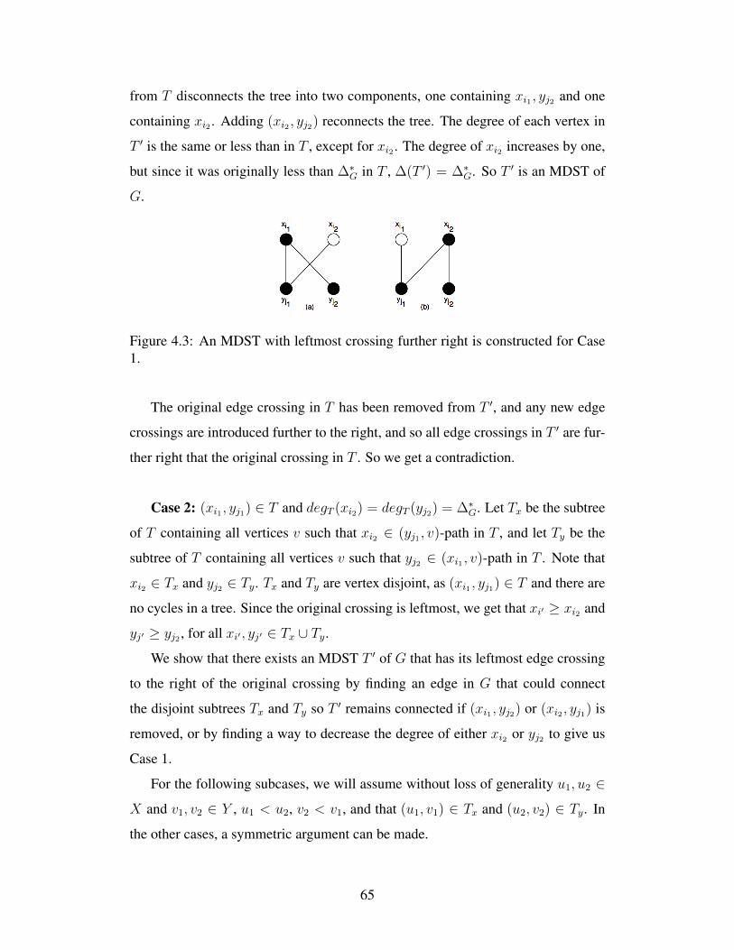
from T disconnects the tree into two components, one containing xi1 , yj2 and one
containing xi2 . Adding (xi2 , yj2) reconnects the tree. The degree of each vertex in
T ′ is the same or less than in T , except for xi2 . The degree of xi2 increases by one,
but since it was originally less than ∆∗G in T , ∆(T ′) = ∆∗G. So T ′ is an MDST of
G.
Figure 4.3: An MDST with leftmost crossing further right is constructed for Case1.
The original edge crossing in T has been removed from T ′, and any new edge
crossings are introduced further to the right, and so all edge crossings in T ′ are fur-
ther right that the original crossing in T . So we get a contradiction.
Case 2: (xi1 , yj1) ∈ T and degT (xi2) = degT (yj2) = ∆∗G. Let Tx be the subtree
of T containing all vertices v such that xi2 ∈ (yj1 , v)-path in T , and let Ty be the
subtree of T containing all vertices v such that yj2 ∈ (xi1 , v)-path in T . Note that
xi2 ∈ Tx and yj2 ∈ Ty. Tx and Ty are vertex disjoint, as (xi1 , yj1) ∈ T and there are
no cycles in a tree. Since the original crossing is leftmost, we get that xi′ ≥ xi2 and
yj′ ≥ yj2 , for all xi′ , yj′ ∈ Tx ∪ Ty.
We show that there exists an MDST T ′ of G that has its leftmost edge crossing
to the right of the original crossing by finding an edge in G that could connect
the disjoint subtrees Tx and Ty so T ′ remains connected if (xi1 , yj2) or (xi2 , yj1) is
removed, or by finding a way to decrease the degree of either xi2 or yj2 to give us
Case 1.
For the following subcases, we will assume without loss of generality u1, u2 ∈
X and v1, v2 ∈ Y , u1 < u2, v2 < v1, and that (u1, v1) ∈ Tx and (u2, v2) ∈ Ty. In
the other cases, a symmetric argument can be made.
65
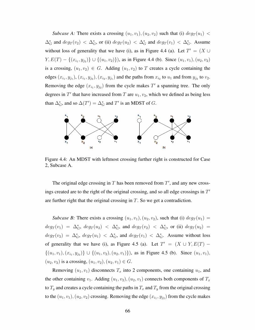
Subcase A: There exists a crossing (u1, v1), (u2, v2) such that (i) degT (u1) <
∆∗G and degT (v2) < ∆∗G, or (ii) degT (u2) < ∆∗G and degT (v1) < ∆∗G. Assume
without loss of generality that we have (i), as in Figure 4.4 (a). Let T ′ = (X ∪
Y,E(T ) − {(xi1 , yj2)} ∪ {(u1, v2)}), as in Figure 4.4 (b). Since (u1, v1), (u2, v2)
is a crossing, (u1, v2) ∈ G. Adding (u1, v2) to T creates a cycle containing the
edges (xi1 , yj1), (xi1 , yj2), (xi2 , yj1) and the paths from xi2 to u1 and from yj2 to v2.
Removing the edge (xi1 , yj2) from the cycle makes T ′ a spanning tree. The only
degrees in T ′ that have increased from T are u1, v2, which we defined as being less
than ∆∗G, and so ∆(T ′) = ∆∗G and T ′ is an MDST of G.
Figure 4.4: An MDST with leftmost crossing further right is constructed for Case2, Subcase A.
The original edge crossing in T has been removed from T ′, and any new cross-
ings created are to the right of the original crossing, and so all edge crossings in T ′
are further right that the original crossing in T . So we get a contradiction.
Subcase B: There exists a crossing (u1, v1), (u2, v2), such that (i) degT (u1) =
degT (v1) = ∆∗G, degT (u2) < ∆∗G, and degT (v2) < ∆∗G, or (ii) degT (u2) =
degT (v2) = ∆∗G, degT (u1) < ∆∗G, and degT (v1) < ∆∗G. Assume without loss
of generality that we have (i), as Figure 4.5 (a). Let T ′ = (X ∪ Y,E(T ) −
{(u1, v1), (xi1 , yj2)} ∪ {(u1, v2), (u2, v1)}), as in Figure 4.5 (b). Since (u1, v1),
(u2, v2) is a crossing, (u1, v2), (u2, v1) ∈ G.
Removing (u1, v1) disconnects Tx into 2 components, one containing u1, and
the other containing v1. Adding (u1, v2), (u2, v1) connects both components of Tx
to Ty and creates a cycle containing the paths in Tx and Ty from the original crossing
to the (u1, v1), (u2, v2) crossing. Removing the edge (xi1 , yj2) from the cycle makes
66
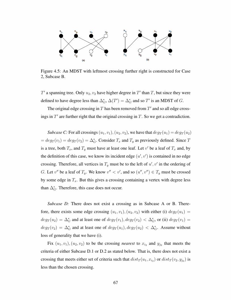
Figure 4.5: An MDST with leftmost crossing further right is constructed for Case2, Subcase B.
T ′ a spanning tree. Only u2, v2 have higher degree in T ′ than T , but since they were
defined to have degree less than ∆∗G, ∆(T ′) = ∆∗G and so T ′ is an MDST of G.
The original edge crossing in T has been removed from T ′ and so all edge cross-
ings in T ′ are further right that the original crossing in T . So we get a contradiction.
Subcase C: For all crossings (u1, v1), (u2, v2), we have that degT (u1) = degT (u2)
= degT (v1) = degT (v2) = ∆∗G. Consider Tx and Ty as previously defined. Since T
is a tree, both Tx, and Ty must have at least one leaf. Let v′ be a leaf of Tx and, by
the definition of this case, we know its incident edge (u′, v′) is contained in no edge
crossing. Therefore, all vertices in Ty must be to the left of u′, v′ in the ordering of
G. Let v′′ be a leaf of Ty. We know v′′ < v′, and so (u′′, v′′) ∈ Ty must be crossed
by some edge in Tx. But this gives a crossing containing a vertex with degree less
than ∆∗G. Therefore, this case does not occur.
Subcase D: There does not exist a crossing as in Subcase A or B. There-
fore, there exists some edge crossing (u1, v1), (u2, v2) with either (i) degT (u1) =
degT (u2) = ∆∗G and at least one of degT (v1), degT (v2) < ∆∗G, or (ii) degT (v1) =
degT (v2) = ∆∗G and at least one of degT (u1), degT (u2) < ∆∗G. Assume without
loss of generality that we have (i).
Fix (u1, v1), (u2, v2) to be the crossing nearest to xi2 and yj2 that meets the
criteria of either Subcase D.1 or D.2 as stated below. That is, there does not exist a
crossing that meets either set of criteria such that distT (u1, xi2) or distT (v2, yj2) is
less than the chosen crossing.
67
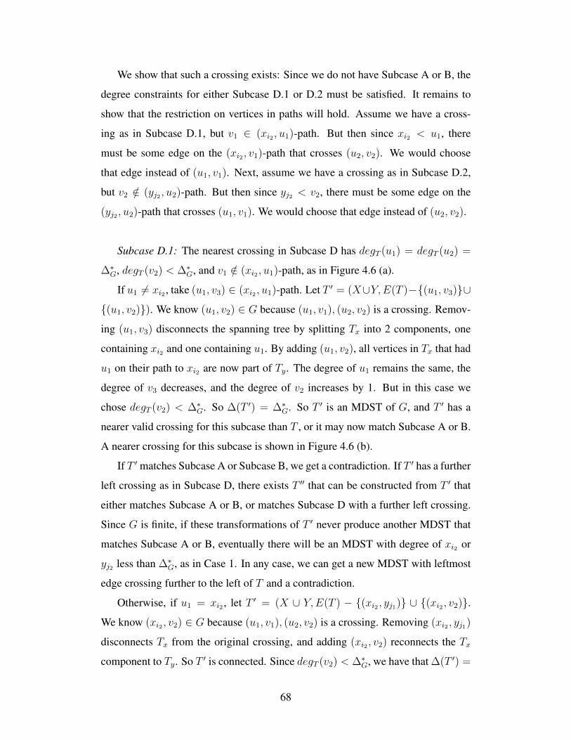
We show that such a crossing exists: Since we do not have Subcase A or B, the
degree constraints for either Subcase D.1 or D.2 must be satisfied. It remains to
show that the restriction on vertices in paths will hold. Assume we have a cross-
ing as in Subcase D.1, but v1 ∈ (xi2 , u1)-path. But then since xi2 < u1, there
must be some edge on the (xi2 , v1)-path that crosses (u2, v2). We would choose
that edge instead of (u1, v1). Next, assume we have a crossing as in Subcase D.2,
but v2 /∈ (yj2 , u2)-path. But then since yj2 < v2, there must be some edge on the
(yj2 , u2)-path that crosses (u1, v1). We would choose that edge instead of (u2, v2).
Subcase D.1: The nearest crossing in Subcase D has degT (u1) = degT (u2) =
∆∗G, degT (v2) < ∆∗G, and v1 /∈ (xi2 , u1)-path, as in Figure 4.6 (a).
If u1 6= xi2 , take (u1, v3) ∈ (xi2 , u1)-path. Let T ′ = (X∪Y,E(T )−{(u1, v3)}∪
{(u1, v2)}). We know (u1, v2) ∈ G because (u1, v1), (u2, v2) is a crossing. Remov-
ing (u1, v3) disconnects the spanning tree by splitting Tx into 2 components, one
containing xi2 and one containing u1. By adding (u1, v2), all vertices in Tx that had
u1 on their path to xi2 are now part of Ty. The degree of u1 remains the same, the
degree of v3 decreases, and the degree of v2 increases by 1. But in this case we
chose degT (v2) < ∆∗G. So ∆(T ′) = ∆∗G. So T ′ is an MDST of G, and T ′ has a
nearer valid crossing for this subcase than T , or it may now match Subcase A or B.
A nearer crossing for this subcase is shown in Figure 4.6 (b).
If T ′ matches Subcase A or Subcase B, we get a contradiction. If T ′ has a further
left crossing as in Subcase D, there exists T ′′ that can be constructed from T ′ that
either matches Subcase A or B, or matches Subcase D with a further left crossing.
Since G is finite, if these transformations of T ′ never produce another MDST that
matches Subcase A or B, eventually there will be an MDST with degree of xi2 or
yj2 less than ∆∗G, as in Case 1. In any case, we can get a new MDST with leftmost
edge crossing further to the left of T and a contradiction.
Otherwise, if u1 = xi2 , let T ′ = (X ∪ Y,E(T ) − {(xi2 , yj1)} ∪ {(xi2 , v2)}.
We know (xi2 , v2) ∈ G because (u1, v1), (u2, v2) is a crossing. Removing (xi2 , yj1)
disconnects Tx from the original crossing, and adding (xi2 , v2) reconnects the Tx
component to Ty. So T ′ is connected. Since degT (v2) < ∆∗G, we have that ∆(T ′) =
68
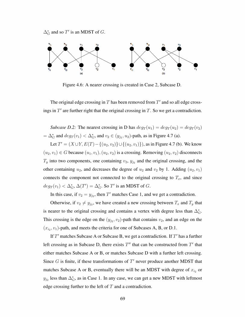
∆∗G and so T ′ is an MDST of G.
Figure 4.6: A nearer crossing is created in Case 2, Subcase D.
The original edge crossing in T has been removed from T ′ and so all edge cross-
ings in T ′ are further right that the original crossing in T . So we get a contradiction.
Subcase D.2: The nearest crossing in D has degT (u1) = degT (u2) = degT (v2)
= ∆∗G and degT (v1) < ∆∗G, and v2 ∈ (yj2 , u2)-path, as in Figure 4.7 (a).
Let T ′ = (X∪Y,E(T )−{(u2, v2)}∪{(u2, v1)}), as in Figure 4.7 (b). We know
(u2, v1) ∈ G because (u1, v1), (u2, v2) is a crossing. Removing (u2, v2) disconnects
Ty into two components, one containing v2, yj2 and the original crossing, and the
other containing u2, and decreases the degree of u2 and v2 by 1. Adding (u2, v1)
connects the component not connected to the original crossing to Tx, and since
degT (v1) < ∆∗G, ∆(T ′) = ∆∗G. So T ′ is an MDST of G.
In this case, if v2 = yj2 , then T ′ matches Case 1, and we get a contradiction.
Otherwise, if v2 6= yj2 , we have created a new crossing between Tx and Ty that
is nearer to the original crossing and contains a vertex with degree less than ∆∗G.
This crossing is the edge on the (yj2 , v2)-path that contains v2, and an edge on the
(xi2 , v1)-path, and meets the criteria for one of Subcases A, B, or D.1.
If T ′ matches Subcase A or Subcase B, we get a contradiction. If T ′ has a further
left crossing as in Subcase D, there exists T ′′ that can be constructed from T ′ that
either matches Subcase A or B, or matches Subcase D with a further left crossing.
Since G is finite, if these transformations of T ′ never produce another MDST that
matches Subcase A or B, eventually there will be an MDST with degree of xi2 or
yj2 less than ∆∗G, as in Case 1. In any case, we can get a new MDST with leftmost
edge crossing further to the left of T and a contradiction.
69
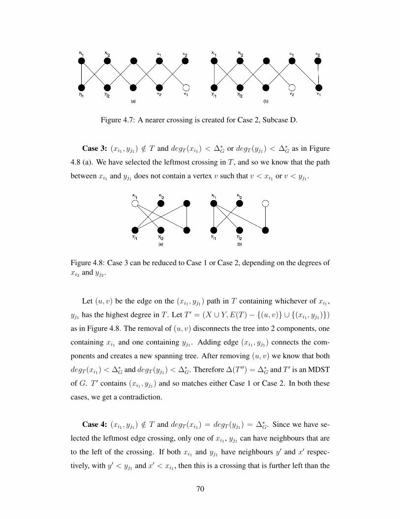
Figure 4.7: A nearer crossing is created for Case 2, Subcase D.
Case 3: (xi1 , yj1) /∈ T and degT (xi1) < ∆∗G or degT (yj1) < ∆∗G as in Figure
4.8 (a). We have selected the leftmost crossing in T , and so we know that the path
between xi1 and yj1 does not contain a vertex v such that v < xi1 or v < yj1 .
Figure 4.8: Case 3 can be reduced to Case 1 or Case 2, depending on the degrees ofxi2 and yj2 .
Let (u, v) be the edge on the (xi1 , yj1) path in T containing whichever of xi1 ,
yj1 has the highest degree in T . Let T ′ = (X ∪ Y,E(T )− {(u, v)} ∪ {(xi1 , yj1)})
as in Figure 4.8. The removal of (u, v) disconnects the tree into 2 components, one
containing xi1 and one containing yj1 . Adding edge (xi1 , yj1) connects the com-
ponents and creates a new spanning tree. After removing (u, v) we know that both
degT (xi1) < ∆∗G and degT (yj1) < ∆∗G. Therefore ∆(T ′′) = ∆∗G and T ′ is an MDST
of G. T ′ contains (xi1 , yj1) and so matches either Case 1 or Case 2. In both these
cases, we get a contradiction.
Case 4: (xi1 , yj1) /∈ T and degT (xi1) = degT (yj1) = ∆∗G. Since we have se-
lected the leftmost edge crossing, only one of xi1 , yj1 can have neighbours that are
to the left of the crossing. If both xi1 and yj1 have neighbours y′ and x′ respec-
tively, with y′ < yj1 and x′ < xi1 , then this is a crossing that is further left than the
70

original crossing. Assume without loss of generality that xi1 is that vertex, and so
∀ v ∈ NT (yj1), v ≥ xi2 .
Subcase A: (xi2 , yj2) /∈ T and xi2 /∈ (yj1 , yj2)-path in T , as in Figure 4.9 (a). Let
T ′ = (X ∪ Y,E(T )− {(xi2 , yj1), (xi1 , yj2)} ∪ {(xi1 , yj1), (xi2 , yj2)}) as in Figure
4.9 (b).
The removal of (xi2 , yj1) divides the tree into 2 components, one containing yj1
and yj2 and one containing xi2 , and reduces the degree of yj1 and xi2 by 1. Remov-
ing (xi1 , yj2) further disconnects the tree into 3 components, the first containing xi1 ,
the second yj1 and yj2 , and the third xi2 , and decreases the degree of xi1 and yj2 .
Adding (xi2 , yj2) connects the first and second components, and adding (xi1 , yj1)
connects the second and third, and since all these vertices had an edge removed,
∆(T ′) = ∆∗G. So T ′ is a minimum degree spanning tree.
Figure 4.9: A new MDST with leftmost edge crossing further right can be con-structed in Case 4, Subcase A.
The original edge crossing in T has been removed from T ′ and so all edge cross-
ings in T ′ are further right that the original crossing in T . So we get a contradiction.
Subcase B: (xi2 , yj2) ∈ T . Let Tx be the subtree of T containing all vertices v
such that xi2 ∈ (yj1 , v)-path, and let Ty be the subtree of T containing all vertices v
such that for some u ∈ NT (yj1)− {xi2}, u ∈ (yj1 , v)-path. So xi2 , yj2 ∈ Tx but not
Ty, and yj1 ∈ Ty.
We proceed with Tx and Ty as in the subcases of Case 2, and construct T ′′. We
have two possibilities for the construction of T ′: first, in Case 2 we are able to
find an edge to add between this Tx and Ty that creates a cycle in T and does not
71
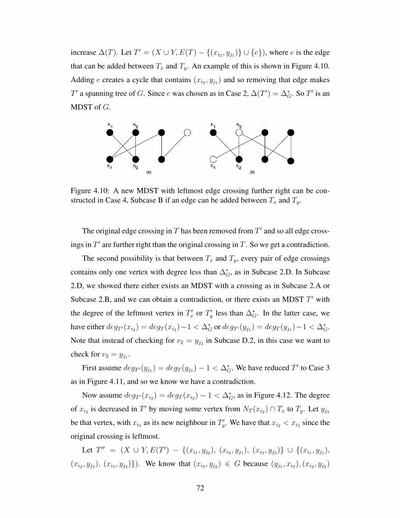
increase ∆(T ). Let T ′ = (X ∪ Y,E(T ) − {(xi2 , yj1)} ∪ {e}), where e is the edge
that can be added between Tx and Ty. An example of this is shown in Figure 4.10.
Adding e creates a cycle that contains (xi2 , yj1) and so removing that edge makes
T ′ a spanning tree of G. Since e was chosen as in Case 2, ∆(T ′) = ∆∗G. So T ′ is an
MDST of G.
Figure 4.10: A new MDST with leftmost edge crossing further right can be con-structed in Case 4, Subcase B if an edge can be added between Tx and Ty.
The original edge crossing in T has been removed from T ′ and so all edge cross-
ings in T ′ are further right than the original crossing in T . So we get a contradiction.
The second possibility is that between Tx and Ty, every pair of edge crossings
contains only one vertex with degree less than ∆∗G, as in Subcase 2.D. In Subcase
2.D, we showed there either exists an MDST with a crossing as in Subcase 2.A or
Subcase 2.B, and we can obtain a contradiction, or there exists an MDST T ′ with
the degree of the leftmost vertex in T ′x or T ′y less than ∆∗G. In the latter case, we
have either degT ′(xi2) = degT (xi2)−1 < ∆∗G or degT ′(yj1) = degT (yj1)−1 < ∆∗G.
Note that instead of checking for v2 = yj2 in Subcase D.2, in this case we want to
check for v2 = yj1 .
First assume degT ′(yj1) = degT (yj1)− 1 < ∆∗G. We have reduced T ′ to Case 3
as in Figure 4.11, and so we know we have a contradiction.
Now assume degT ′(xi2) = degT (xi2)− 1 < ∆∗G, as in Figure 4.12. The degree
of xi2 is decreased in T ′ by moving some vertex from NT (xi2) ∩ Tx to Ty. Let yj3
be that vertex, with xi3 as its new neighbour in T ′y. We have that xi2 < xi3 since the
original crossing is leftmost.
Let T ′′ = (X ∪ Y,E(T ′) − {(xi1 , yj2), (xi2 , yj1), (xi3 , yj3)} ∪ {(xi1 , yj1),
(xi2 , yj3), (xi3 , yj2)}). We know that (xi3 , yj2) ∈ G because (yj1 , xi3), (xi2 , yj2)
72
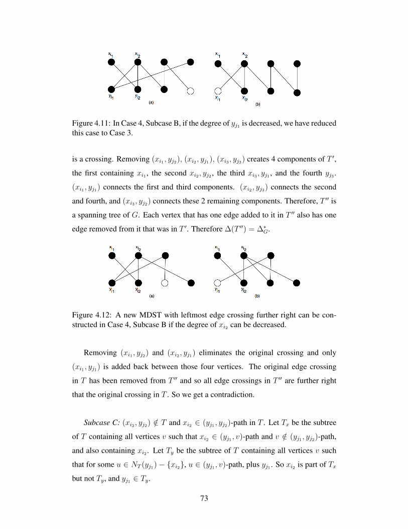
Figure 4.11: In Case 4, Subcase B, if the degree of yj1 is decreased, we have reducedthis case to Case 3.
is a crossing. Removing (xi1 , yj2), (xi2 , yj1), (xi3 , yj3) creates 4 components of T ′,
the first containing xi1 , the second xi2 , yj2 , the third xi3 , yj1 , and the fourth yj3 .
(xi1 , yj1) connects the first and third components. (xi2 , yj3) connects the second
and fourth, and (xi3 , yj2) connects these 2 remaining components. Therefore, T ′′ is
a spanning tree of G. Each vertex that has one edge added to it in T ′′ also has one
edge removed from it that was in T ′. Therefore ∆(T ′′) = ∆∗G.
Figure 4.12: A new MDST with leftmost edge crossing further right can be con-structed in Case 4, Subcase B if the degree of xi2 can be decreased.
Removing (xi1 , yj2) and (xi2 , yj1) eliminates the original crossing and only
(xi1 , yj1) is added back between those four vertices. The original edge crossing
in T has been removed from T ′′ and so all edge crossings in T ′′ are further right
that the original crossing in T . So we get a contradiction.
Subcase C: (xi2 , yj2) /∈ T and xi2 ∈ (yj1 , yj2)-path in T . Let Tx be the subtree
of T containing all vertices v such that xi2 ∈ (yj1 , v)-path and v /∈ (yj1 , yj2)-path,
and also containing xi2 . Let Ty be the subtree of T containing all vertices v such
that for some u ∈ NT (yj1)− {xi2}, u ∈ (yj1 , v)-path, plus yj1 . So xi2 is part of Tx
but not Ty, and yj1 ∈ Ty.
73
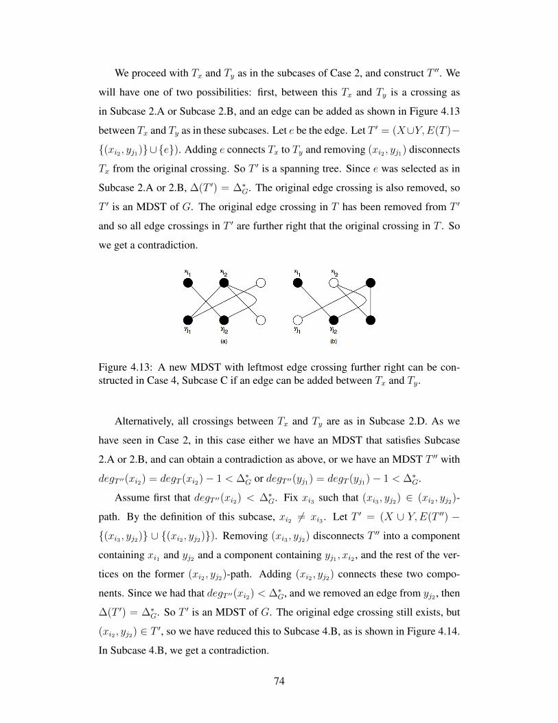
We proceed with Tx and Ty as in the subcases of Case 2, and construct T ′′. We
will have one of two possibilities: first, between this Tx and Ty is a crossing as
in Subcase 2.A or Subcase 2.B, and an edge can be added as shown in Figure 4.13
between Tx and Ty as in these subcases. Let e be the edge. Let T ′ = (X∪Y,E(T )−
{(xi2 , yj1)}∪{e}). Adding e connects Tx to Ty and removing (xi2 , yj1) disconnects
Tx from the original crossing. So T ′ is a spanning tree. Since e was selected as in
Subcase 2.A or 2.B, ∆(T ′) = ∆∗G. The original edge crossing is also removed, so
T ′ is an MDST of G. The original edge crossing in T has been removed from T ′
and so all edge crossings in T ′ are further right that the original crossing in T . So
we get a contradiction.
Figure 4.13: A new MDST with leftmost edge crossing further right can be con-structed in Case 4, Subcase C if an edge can be added between Tx and Ty.
Alternatively, all crossings between Tx and Ty are as in Subcase 2.D. As we
have seen in Case 2, in this case either we have an MDST that satisfies Subcase
2.A or 2.B, and can obtain a contradiction as above, or we have an MDST T ′′ with
degT ′′(xi2) = degT (xi2)− 1 < ∆∗G or degT ′′(yj1) = degT (yj1)− 1 < ∆∗G.
Assume first that degT ′′(xi2) < ∆∗G. Fix xi3 such that (xi3 , yj2) ∈ (xi2 , yj2)-
path. By the definition of this subcase, xi2 6= xi3 . Let T ′ = (X ∪ Y,E(T ′′) −
{(xi3 , yj2)} ∪ {(xi2 , yj2)}). Removing (xi3 , yj2) disconnects T ′′ into a component
containing xi1 and yj2 and a component containing yj1 , xi2 , and the rest of the ver-
tices on the former (xi2 , yj2)-path. Adding (xi2 , yj2) connects these two compo-
nents. Since we had that degT ′′(xi2) < ∆∗G, and we removed an edge from yj2 , then
∆(T ′) = ∆∗G. So T ′ is an MDST of G. The original edge crossing still exists, but
(xi2 , yj2) ∈ T ′, so we have reduced this to Subcase 4.B, as is shown in Figure 4.14.
In Subcase 4.B, we get a contradiction.
74
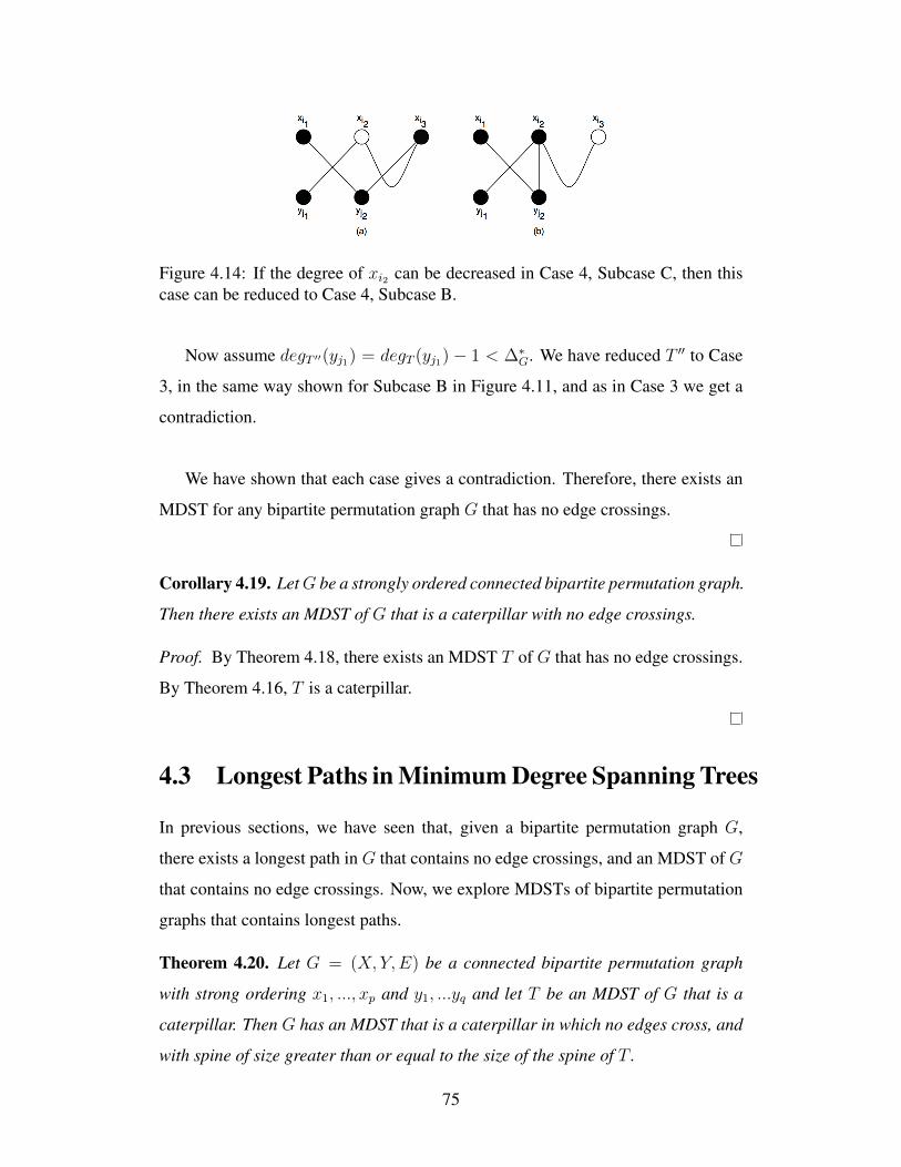
Figure 4.14: If the degree of xi2 can be decreased in Case 4, Subcase C, then thiscase can be reduced to Case 4, Subcase B.
Now assume degT ′′(yj1) = degT (yj1) − 1 < ∆∗G. We have reduced T ′′ to Case
3, in the same way shown for Subcase B in Figure 4.11, and as in Case 3 we get a
contradiction.
We have shown that each case gives a contradiction. Therefore, there exists an
MDST for any bipartite permutation graph G that has no edge crossings.
Corollary 4.19. LetG be a strongly ordered connected bipartite permutation graph.
Then there exists an MDST of G that is a caterpillar with no edge crossings.
Proof. By Theorem 4.18, there exists an MDST T of G that has no edge crossings.
By Theorem 4.16, T is a caterpillar.
4.3 Longest Paths in Minimum Degree Spanning Trees
In previous sections, we have seen that, given a bipartite permutation graph G,
there exists a longest path in G that contains no edge crossings, and an MDST of G
that contains no edge crossings. Now, we explore MDSTs of bipartite permutation
graphs that contains longest paths.
Theorem 4.20. Let G = (X, Y,E) be a connected bipartite permutation graph
with strong ordering x1, ..., xp and y1, ...yq and let T be an MDST of G that is a
caterpillar. Then G has an MDST that is a caterpillar in which no edges cross, and
with spine of size greater than or equal to the size of the spine of T .
75
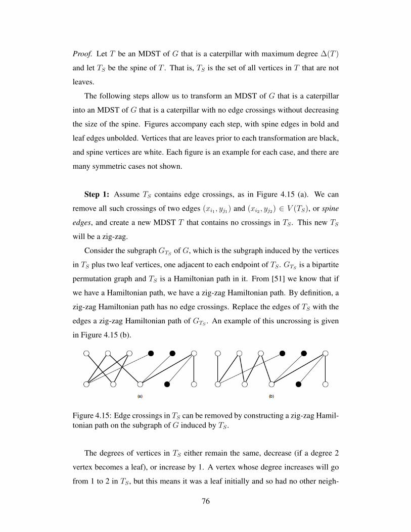
Proof. Let T be an MDST of G that is a caterpillar with maximum degree ∆(T )
and let TS be the spine of T . That is, TS is the set of all vertices in T that are not
leaves.
The following steps allow us to transform an MDST of G that is a caterpillar
into an MDST of G that is a caterpillar with no edge crossings without decreasing
the size of the spine. Figures accompany each step, with spine edges in bold and
leaf edges unbolded. Vertices that are leaves prior to each transformation are black,
and spine vertices are white. Each figure is an example for each case, and there are
many symmetric cases not shown.
Step 1: Assume TS contains edge crossings, as in Figure 4.15 (a). We can
remove all such crossings of two edges (xi1 , yj1) and (xi2 , yj2) ∈ V (TS), or spine
edges, and create a new MDST T that contains no crossings in TS . This new TS
will be a zig-zag.
Consider the subgraph GTS of G, which is the subgraph induced by the vertices
in TS plus two leaf vertices, one adjacent to each endpoint of TS . GTS is a bipartite
permutation graph and TS is a Hamiltonian path in it. From [51] we know that if
we have a Hamiltonian path, we have a zig-zag Hamiltonian path. By definition, a
zig-zag Hamiltonian path has no edge crossings. Replace the edges of TS with the
edges a zig-zag Hamiltonian path of GTS . An example of this uncrossing is given
in Figure 4.15 (b).
Figure 4.15: Edge crossings in TS can be removed by constructing a zig-zag Hamil-tonian path on the subgraph of G induced by TS .
The degrees of vertices in TS either remain the same, decrease (if a degree 2
vertex becomes a leaf), or increase by 1. A vertex whose degree increases will go
from 1 to 2 in TS , but this means it was a leaf initially and so had no other neigh-
76
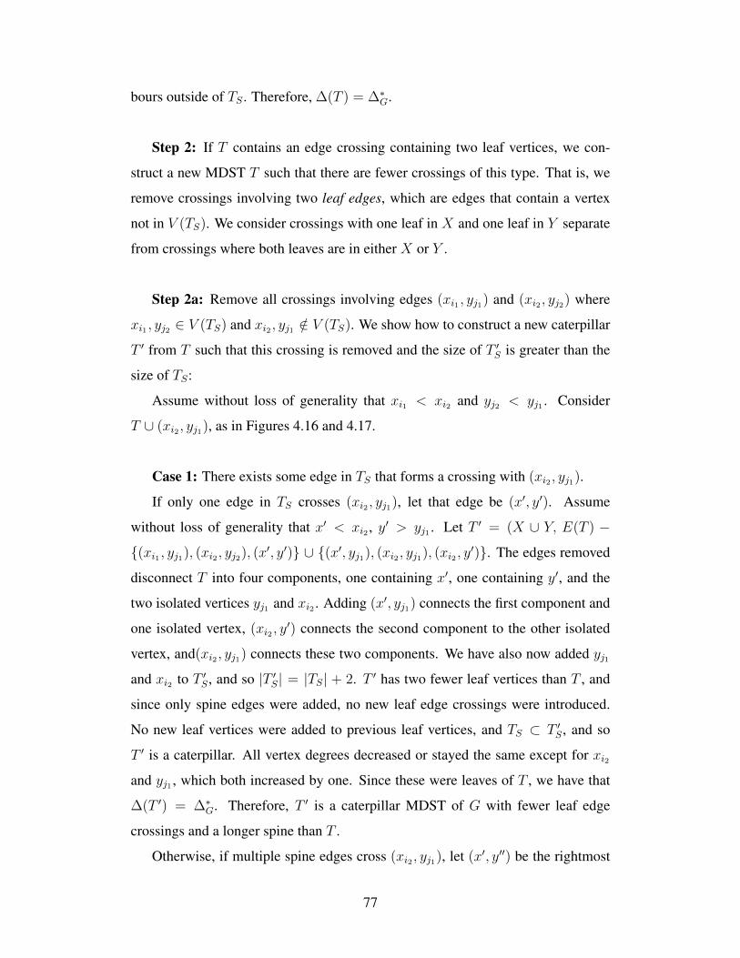
bours outside of TS . Therefore, ∆(T ) = ∆∗G.
Step 2: If T contains an edge crossing containing two leaf vertices, we con-
struct a new MDST T such that there are fewer crossings of this type. That is, we
remove crossings involving two leaf edges, which are edges that contain a vertex
not in V (TS). We consider crossings with one leaf in X and one leaf in Y separate
from crossings where both leaves are in either X or Y .
Step 2a: Remove all crossings involving edges (xi1 , yj1) and (xi2 , yj2) where
xi1 , yj2 ∈ V (TS) and xi2 , yj1 /∈ V (TS). We show how to construct a new caterpillar
T ′ from T such that this crossing is removed and the size of T ′S is greater than the
size of TS:
Assume without loss of generality that xi1 < xi2 and yj2 < yj1 . Consider
T ∪ (xi2 , yj1), as in Figures 4.16 and 4.17.
Case 1: There exists some edge in TS that forms a crossing with (xi2 , yj1).
If only one edge in TS crosses (xi2 , yj1), let that edge be (x′, y′). Assume
without loss of generality that x′ < xi2 , y′ > yj1 . Let T ′ = (X ∪ Y, E(T ) −
{(xi1 , yj1), (xi2 , yj2), (x′, y′)} ∪ {(x′, yj1), (xi2 , yj1), (xi2 , y′)}. The edges removed
disconnect T into four components, one containing x′, one containing y′, and the
two isolated vertices yj1 and xi2 . Adding (x′, yj1) connects the first component and
one isolated vertex, (xi2 , y′) connects the second component to the other isolated
vertex, and(xi2 , yj1) connects these two components. We have also now added yj1
and xi2 to T ′S , and so |T ′S| = |TS| + 2. T ′ has two fewer leaf vertices than T , and
since only spine edges were added, no new leaf edge crossings were introduced.
No new leaf vertices were added to previous leaf vertices, and TS ⊂ T ′S , and so
T ′ is a caterpillar. All vertex degrees decreased or stayed the same except for xi2
and yj1 , which both increased by one. Since these were leaves of T , we have that
∆(T ′) = ∆∗G. Therefore, T ′ is a caterpillar MDST of G with fewer leaf edge
crossings and a longer spine than T .
Otherwise, if multiple spine edges cross (xi2 , yj1), let (x′, y′′) be the rightmost
77
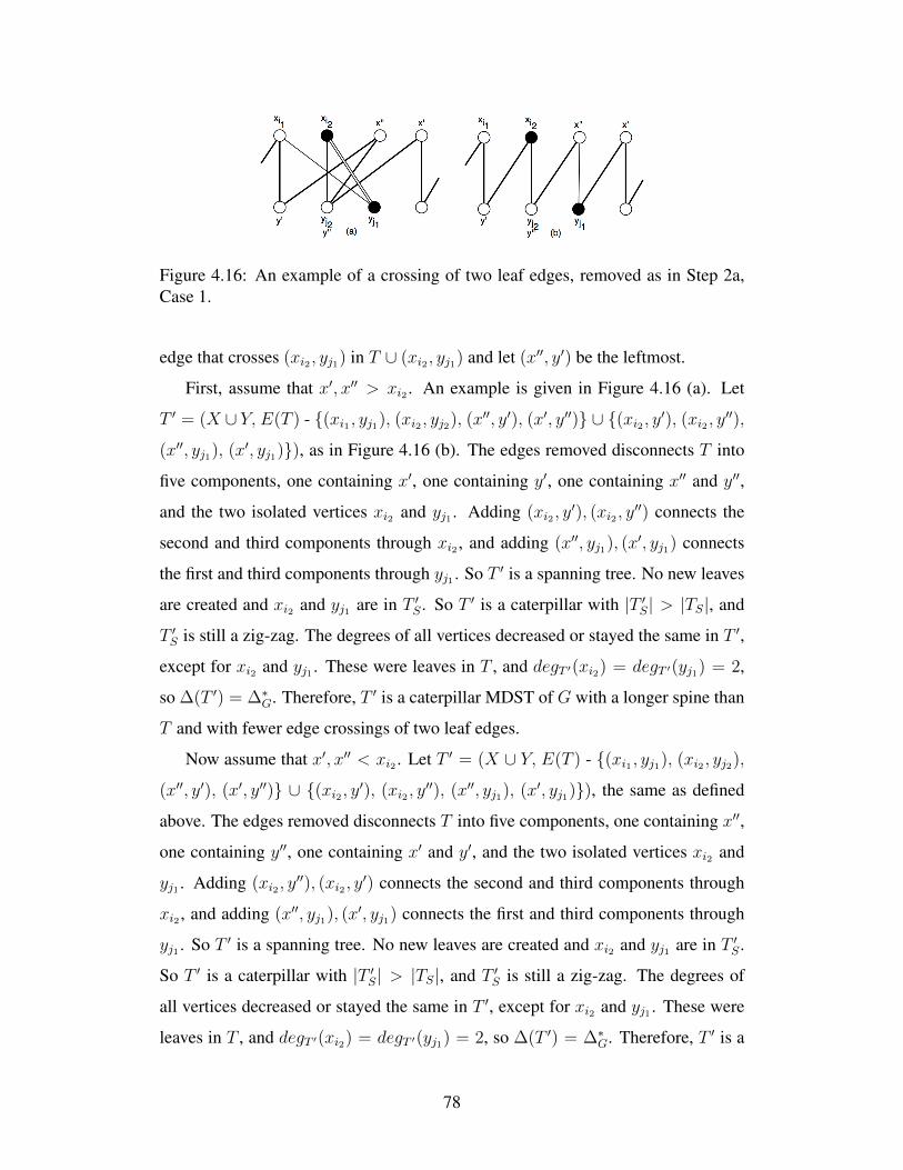
Figure 4.16: An example of a crossing of two leaf edges, removed as in Step 2a,Case 1.
edge that crosses (xi2 , yj1) in T ∪ (xi2 , yj1) and let (x′′, y′) be the leftmost.
First, assume that x′, x′′ > xi2 . An example is given in Figure 4.16 (a). Let
T ′ = (X ∪ Y, E(T ) - {(xi1 , yj1), (xi2 , yj2), (x′′, y′), (x′, y′′)} ∪ {(xi2 , y′), (xi2 , y′′),
(x′′, yj1), (x′, yj1)}), as in Figure 4.16 (b). The edges removed disconnects T into
five components, one containing x′, one containing y′, one containing x′′ and y′′,
and the two isolated vertices xi2 and yj1 . Adding (xi2 , y′), (xi2 , y
′′) connects the
second and third components through xi2 , and adding (x′′, yj1), (x′, yj1) connects
the first and third components through yj1 . So T ′ is a spanning tree. No new leaves
are created and xi2 and yj1 are in T ′S . So T ′ is a caterpillar with |T ′S| > |TS|, and
T ′S is still a zig-zag. The degrees of all vertices decreased or stayed the same in T ′,
except for xi2 and yj1 . These were leaves in T , and degT ′(xi2) = degT ′(yj1) = 2,
so ∆(T ′) = ∆∗G. Therefore, T ′ is a caterpillar MDST of G with a longer spine than
T and with fewer edge crossings of two leaf edges.
Now assume that x′, x′′ < xi2 . Let T ′ = (X ∪ Y, E(T ) - {(xi1 , yj1), (xi2 , yj2),
(x′′, y′), (x′, y′′)} ∪ {(xi2 , y′), (xi2 , y′′), (x′′, yj1), (x′, yj1)}), the same as defined
above. The edges removed disconnects T into five components, one containing x′′,
one containing y′′, one containing x′ and y′, and the two isolated vertices xi2 and
yj1 . Adding (xi2 , y′′), (xi2 , y
′) connects the second and third components through
xi2 , and adding (x′′, yj1), (x′, yj1) connects the first and third components through
yj1 . So T ′ is a spanning tree. No new leaves are created and xi2 and yj1 are in T ′S .
So T ′ is a caterpillar with |T ′S| > |TS|, and T ′S is still a zig-zag. The degrees of
all vertices decreased or stayed the same in T ′, except for xi2 and yj1 . These were
leaves in T , and degT ′(xi2) = degT ′(yj1) = 2, so ∆(T ′) = ∆∗G. Therefore, T ′ is a
78
caterpillar MDST of G with a longer spine than T and with fewer edge crossings of
two leaf edges.
In this case, it is possible that T ′ contains edge crossings between edges added
to the spine. However, from Step 1 we know there exists another MDST that is a
caterpillar with the same spine as T ′ that contains no spine edge crossings.
Case 2: No edge in TS forms a crossing with (xi2 , yj1). Recall our assumption
that xi1 < xi2 and yj2 < yj1 . Since TS is a zig-zag after Step 1, then xi2 or yj1 must
be adjacent in G to the rightmost endpoint of TS (or leftmost if we had assumed
xi1 > xi2). Note that an endpoint of TS is not a leaf in T . Assume without loss of
generality that the rightmost endpoint of TS is in Y . Let yj3 be this endpoint.
If yj2 = yj3 , let T ′ = (X ∪ Y,E(T ) − {(xi1 , yj1)} ∪ {(xi2 , yj1)}. yj1 is now
an endpoint of T ′S and xi2 is now in T ′S as a middle vertex. Since xi2 was an end-
point, T ′ is also a caterpillar. After removing (xi1 , yj1), yj1 becomes an isolated
vertex. Adding (xi2 , yj1) reconnects it to the graph. All vertex degrees decrease or
remain the same, except for yj1 . Since degT (yj1) = 1, we get degT ′(yj1) = 2 and
so ∆(T ′) = ∆∗G. Therefore T ′ is a caterpillar MDST of G with one fewer edge
crossing involving two leaf vertices, and |T ′S| > |TS|.
Otherwise yj2 < yj3 , as in Figure 4.17 (a). Since yj3 is the endpoint of TS and
has degree at least 2, and we have completed Step 1, we know that yj3 must have at
least one leaf in T that does not cross any edge in TS . Let xi3 be this leaf. We have
two cases for the ordering of xi2 , xi3 .
If xi3 < xi2 , then let T ′ = (X ∪ Y, E(T ) − {(xi1 , yj1), (xi2 , yj2)} ∪ {(xi3 , yj1),
(xi2 , yj1)}, as in Figure 4.17 (b). Since (xi3 , yj3) does not cross any other spine
edges, we must have that (xi3 , yj3), (xi1 , yj1) is an edge crossing in T . Therefore
we know that (xi3 , yj1) ∈ E(G). xi3 was a leaf of an endpoint of TS , and so adding
yj1 as its neighbour makes it a new endpoint of the spine with yj1 as a leaf. Simi-
larly, yj1 becomes an endpoint with xi2 as a leaf. So T ′ is a caterpillar. Additionally,
a crossing of two leaf edges has been removed. Removing (xi1 , yj1), (xi2 , yj2) dis-
connects T into three components, two of which are the isolated vertices xi2 , yj1 .
Adding (xi3 , yj1) connects yj1 to the rest of the tree, and adding (xi2 , yj1) connects
79
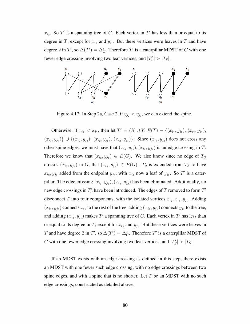
xi2 . So T ′ is a spanning tree of G. Each vertex in T ′ has less than or equal to its
degree in T , except for xi3 and yj1 . But these vertices were leaves in T and have
degree 2 in T ′, so ∆(T ′) = ∆∗G. Therefore T ′ is a caterpillar MDST of G with one
fewer edge crossing involving two leaf vertices, and |T ′S| > |TS|.
Figure 4.17: In Step 2a, Case 2, if yj2 < yj3 , we can extend the spine.
Otherwise, if xi2 < xi3 , then let T ′ = (X ∪ Y, E(T ) − {(xi1 , yj1), (xi2 , yj2),
(xi3 , yj3)} ∪ {(xi2 , yj3), (xi2 , yj1), (xi3 , yj1)}. Since (xi3 , yj3) does not cross any
other spine edges, we must have that (xi3 , yj3), (xi1 , yj1) is an edge crossing in T .
Therefore we know that (xi3 , yj1) ∈ E(G). We also know since no edge of TS
crosses (xi2 , yj1) in G, that (xi2 , yj3) ∈ E(G). T ′S is extended from TS to have
xi2 , yj1 added from the endpoint yj3 , with xi3 now a leaf of yj1 . So T ′ is a cater-
pillar. The edge crossing (xi1 , yj1), (xi2 , yj2) has been eliminated. Additionally, no
new edge crossings in T ′S have been introduced. The edges of T removed to form T ′
disconnect T into four components, with the isolated vertices xi2 , xi3 , yj1 . Adding
(xi2 , yj3) connects xi2 to the rest of the tree, adding (xi2 , yj1) connects yj1 to the tree,
and adding (xi3 , yj1) makes T ′ a spanning tree of G. Each vertex in T ′ has less than
or equal to its degree in T , except for xi2 and yj1 . But these vertices were leaves in
T and have degree 2 in T ′, so ∆(T ′) = ∆∗G. Therefore T ′ is a caterpillar MDST of
G with one fewer edge crossing involving two leaf vertices, and |T ′S| > |TS|.
If an MDST exists with an edge crossing as defined in this step, there exists
an MDST with one fewer such edge crossing, with no edge crossings between two
spine edges, and with a spine that is no shorter. Let T be an MDST with no such
edge crossings, constructed as detailed above.
80
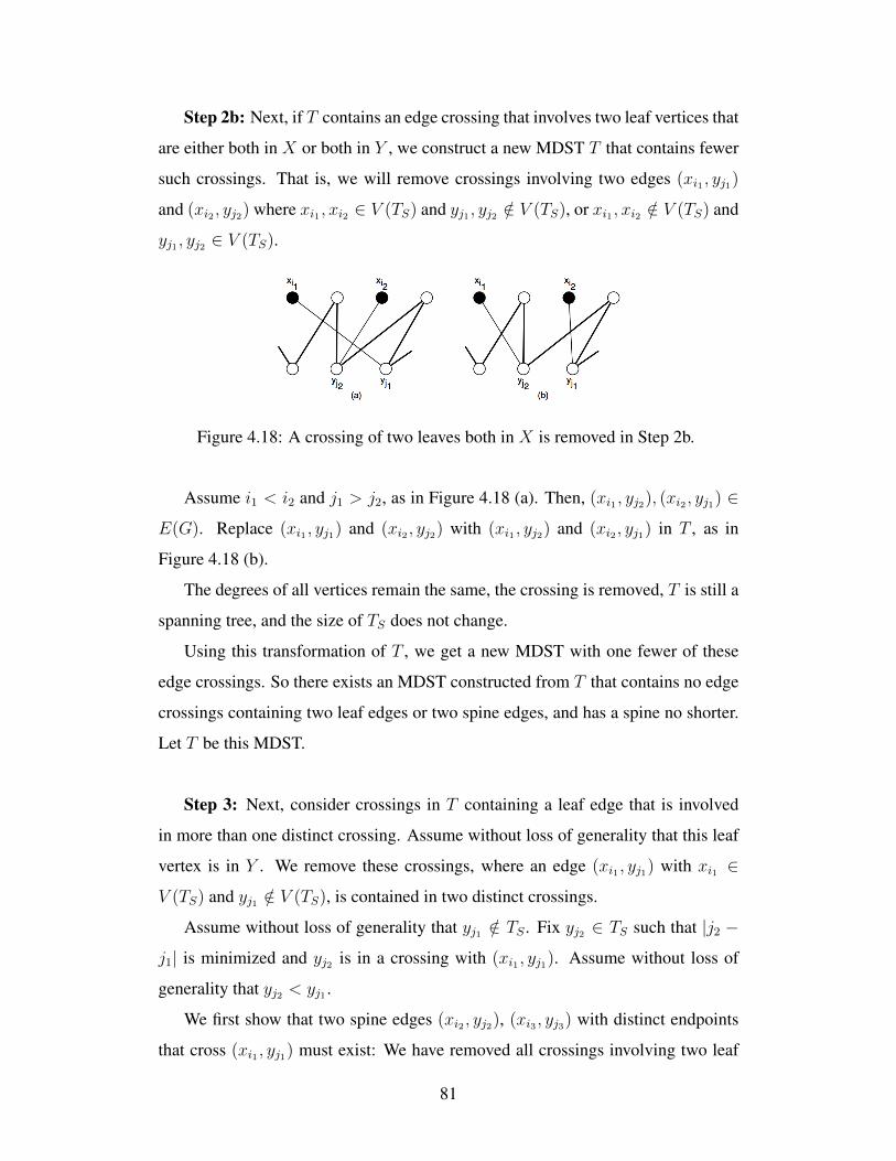
Step 2b: Next, if T contains an edge crossing that involves two leaf vertices that
are either both in X or both in Y , we construct a new MDST T that contains fewer
such crossings. That is, we will remove crossings involving two edges (xi1 , yj1)
and (xi2 , yj2) where xi1 , xi2 ∈ V (TS) and yj1 , yj2 /∈ V (TS), or xi1 , xi2 /∈ V (TS) and
yj1 , yj2 ∈ V (TS).
Figure 4.18: A crossing of two leaves both in X is removed in Step 2b.
Assume i1 < i2 and j1 > j2, as in Figure 4.18 (a). Then, (xi1 , yj2), (xi2 , yj1) ∈
E(G). Replace (xi1 , yj1) and (xi2 , yj2) with (xi1 , yj2) and (xi2 , yj1) in T , as in
Figure 4.18 (b).
The degrees of all vertices remain the same, the crossing is removed, T is still a
spanning tree, and the size of TS does not change.
Using this transformation of T , we get a new MDST with one fewer of these
edge crossings. So there exists an MDST constructed from T that contains no edge
crossings containing two leaf edges or two spine edges, and has a spine no shorter.
Let T be this MDST.
Step 3: Next, consider crossings in T containing a leaf edge that is involved
in more than one distinct crossing. Assume without loss of generality that this leaf
vertex is in Y . We remove these crossings, where an edge (xi1 , yj1) with xi1 ∈
V (TS) and yj1 /∈ V (TS), is contained in two distinct crossings.
Assume without loss of generality that yj1 /∈ TS . Fix yj2 ∈ TS such that |j2 −
j1| is minimized and yj2 is in a crossing with (xi1 , yj1). Assume without loss of
generality that yj2 < yj1 .
We first show that two spine edges (xi2 , yj2), (xi3 , yj3) with distinct endpoints
that cross (xi1 , yj1) must exist: We have removed all crossings involving two leaf
81
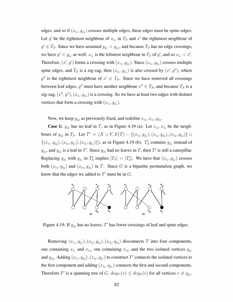
edges, and so if (xi1 , yj1) crosses multiple edges, these edges must be spine edges.
Let y′ be the rightmost neighbour of xi1 in TS and x′ the rightmost neighbour of
y′ ∈ TS . Since we have assumed yj2 < yj1 , and because TS has no edge crossings,
we have y′ < yj1 as well. xi1 is the leftmost neighbour in TS of y′, and so xi1 < x′.
Therefore, (x′, y′) forms a crossing with (xi1 , yj1). Since (xi1 , yj1) crosses multiple
spine edges, and TS is a zig-zag, then (xi1 , yj1) is also crossed by (x′, y′′), where
y′′ is the rightmost neighbour of x′ ∈ TS . Since we have removed all crossings
between leaf edges, y′′ must have another neighbour x′′ ∈ TS , and because TS is a
zig-zag, (x′′, y′′), (xi1 , yj1) is a crossing. So we have at least two edges with distinct
vertices that form a crossing with (xi1 , yj1).
Now, we keep yj2 as previously fixed, and redefine xi2 , xi3 , yj3 .
Case 1: yj2 has no leaf in T , as in Figure 4.19 (a). Let xi2 , xi3 be the neigh-
bours of yj2 in TS . Let T ′ = (X ∪ Y,E(T ) − {(xi1 , yj1), (xi2 , yj2), (xi3 , yj2)} ∪
{(xi1 , yj2), (xi2 , yj1), (xi3 , yj1)}), as in Figure 4.19 (b). T ′S contains yj1 instead of
yj2 , and yj2 is a leaf in T ′. Since yj2 had no leaves in T , then T ′ is still a caterpillar.
Replacing yj2 with yj1 in T ′S implies |TS| = |T ′S|. We have that (xi1 , yj1) crosses
both (xi2 , yj2) and (xi3 , yj2) in T . Since G is a bipartite permutation graph, we
know that the edges we added to T ′ must be in G.
Figure 4.19: If yj2 has no leaves, T ′ has fewer crossings of leaf and spine edges.
Removing (xi1 , yj1), (xi2 , yj2), (xi3 , yj2) disconnects T into four components,
one containing xi1 and xi2 , one containing xi3 , and the two isolated vertices yj1
and yj2 . Adding (xi1 , yj2), (xi2 , yj1) to construct T ′ connects the isolated vertices to
the first component and adding (xi3 , yj1) connects the first and second components.
Therefore T ′ is a spanning tree of G. degT ′(v) ≤ degT (v) for all vertices v 6= yj1 .
82
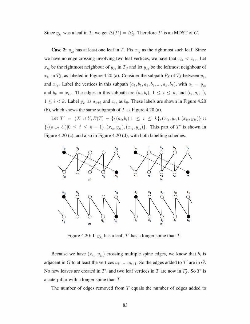
Since yj1 was a leaf in T , we get ∆(T ′) = ∆∗G. Therefore T ′ is an MDST of G.
Case 2: yj2 has at least one leaf in T . Fix xi2 as the rightmost such leaf. Since
we have no edge crossing involving two leaf vertices, we have that xi2 < xi1 . Let
xi3 be the rightmost neighbour of yj2 in TS and let yj3 be the leftmost neighbour of
xi1 in TS , as labeled in Figure 4.20 (a). Consider the subpath PS of TS between yj3
and xi3 . Label the vertices in this subpath (a1, b1, a2, b2, ..., ak, bk), with a1 = yj3
and bk = xi3 . The edges in this subpath are (ai, bi), 1 ≤ i ≤ k, and (bi, ai+1),
1 ≤ i < k. Label yj1 as ak+1 and xi2 as b0. These labels are shown in Figure 4.20
(b), which shows the same subgraph of T as Figure 4.20 (a).
Let T ′ = (X ∪ Y,E(T ) − {{(ai, bi)|1 ≤ i ≤ k}, (xi1 , yj1), (xi2 , yj2)} ∪
{{(ai+2, bi)|0 ≤ i ≤ k − 1}, (xi3 , yj1), (xi2 , yj3)}. This part of T ′ is shown in
Figure 4.20 (c), and also in Figure 4.20 (d), with both labelling schemes.
Figure 4.20: If yj2 has a leaf, T ′ has a longer spine than T .
Because we have (xi1 , yj1) crossing multiple spine edges, we know that bi is
adjacent in G to at least the vertices ai, ..., ak+1. So the edges added to T ′ are in G.
No new leaves are created in T ′, and two leaf vertices in T are now in T ′S . So T ′ is
a caterpillar with a longer spine than T .
The number of edges removed from T equals the number of edges added to
83
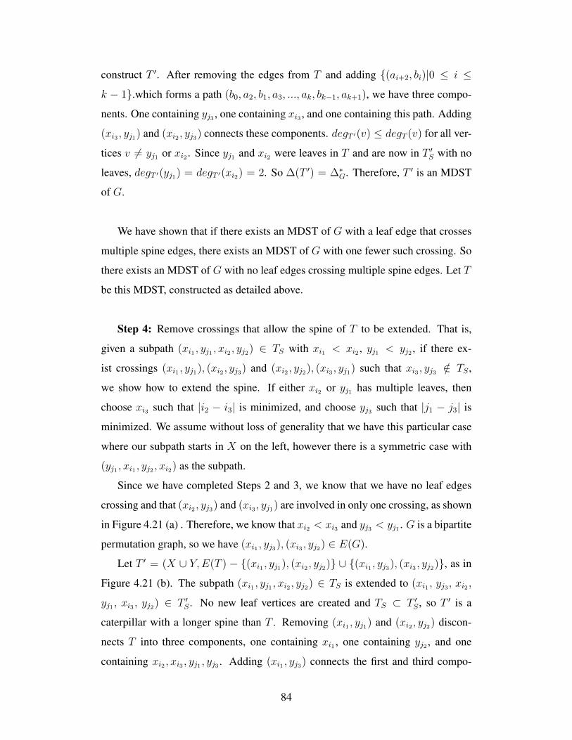
construct T ′. After removing the edges from T and adding {(ai+2, bi)|0 ≤ i ≤
k − 1}.which forms a path (b0, a2, b1, a3, ..., ak, bk−1, ak+1), we have three compo-
nents. One containing yj3 , one containing xi3 , and one containing this path. Adding
(xi3 , yj1) and (xi2 , yj3) connects these components. degT ′(v) ≤ degT (v) for all ver-
tices v 6= yj1 or xi2 . Since yj1 and xi2 were leaves in T and are now in T ′S with no
leaves, degT ′(yj1) = degT ′(xi2) = 2. So ∆(T ′) = ∆∗G. Therefore, T ′ is an MDST
of G.
We have shown that if there exists an MDST of G with a leaf edge that crosses
multiple spine edges, there exists an MDST of G with one fewer such crossing. So
there exists an MDST of G with no leaf edges crossing multiple spine edges. Let T
be this MDST, constructed as detailed above.
Step 4: Remove crossings that allow the spine of T to be extended. That is,
given a subpath (xi1 , yj1 , xi2 , yj2) ∈ TS with xi1 < xi2 , yj1 < yj2 , if there ex-
ist crossings (xi1 , yj1), (xi2 , yj3) and (xi2 , yj2), (xi3 , yj1) such that xi3 , yj3 /∈ TS ,
we show how to extend the spine. If either xi2 or yj1 has multiple leaves, then
choose xi3 such that |i2 − i3| is minimized, and choose yj3 such that |j1 − j3| is
minimized. We assume without loss of generality that we have this particular case
where our subpath starts in X on the left, however there is a symmetric case with
(yj1 , xi1 , yj2 , xi2) as the subpath.
Since we have completed Steps 2 and 3, we know that we have no leaf edges
crossing and that (xi2 , yj3) and (xi3 , yj1) are involved in only one crossing, as shown
in Figure 4.21 (a) . Therefore, we know that xi2 < xi3 and yj3 < yj1 . G is a bipartite
permutation graph, so we have (xi1 , yj3), (xi3 , yj2) ∈ E(G).
Let T ′ = (X ∪ Y,E(T ) − {(xi1 , yj1), (xi2 , yj2)} ∪ {(xi1 , yj3), (xi3 , yj2)}, as in
Figure 4.21 (b). The subpath (xi1 , yj1 , xi2 , yj2) ∈ TS is extended to (xi1 , yj3 , xi2 ,
yj1 , xi3 , yj2) ∈ T ′S . No new leaf vertices are created and TS ⊂ T ′S , so T ′ is a
caterpillar with a longer spine than T . Removing (xi1 , yj1) and (xi2 , yj2) discon-
nects T into three components, one containing xi1 , one containing yj2 , and one
containing xi2 , xi3 , yj1 , yj3 . Adding (xi1 , yj3) connects the first and third compo-
84
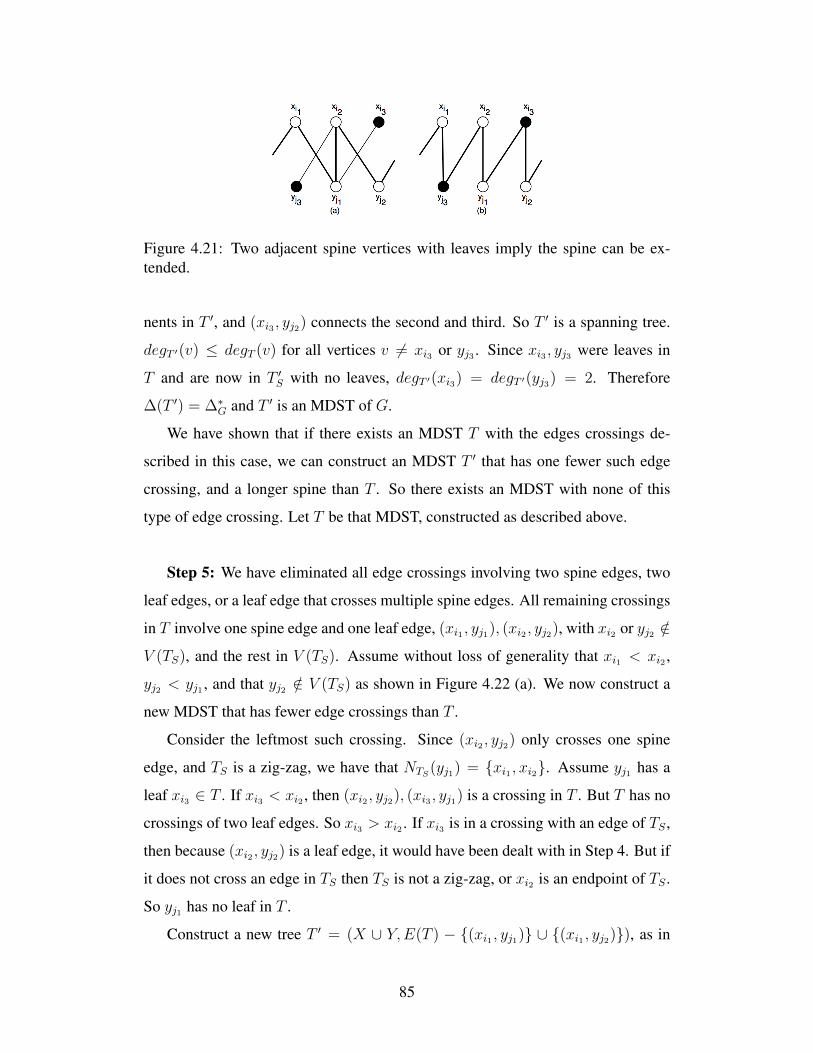
Figure 4.21: Two adjacent spine vertices with leaves imply the spine can be ex-tended.
nents in T ′, and (xi3 , yj2) connects the second and third. So T ′ is a spanning tree.
degT ′(v) ≤ degT (v) for all vertices v 6= xi3 or yj3 . Since xi3 , yj3 were leaves in
T and are now in T ′S with no leaves, degT ′(xi3) = degT ′(yj3) = 2. Therefore
∆(T ′) = ∆∗G and T ′ is an MDST of G.
We have shown that if there exists an MDST T with the edges crossings de-
scribed in this case, we can construct an MDST T ′ that has one fewer such edge
crossing, and a longer spine than T . So there exists an MDST with none of this
type of edge crossing. Let T be that MDST, constructed as described above.
Step 5: We have eliminated all edge crossings involving two spine edges, two
leaf edges, or a leaf edge that crosses multiple spine edges. All remaining crossings
in T involve one spine edge and one leaf edge, (xi1 , yj1), (xi2 , yj2), with xi2 or yj2 /∈
V (TS), and the rest in V (TS). Assume without loss of generality that xi1 < xi2 ,
yj2 < yj1 , and that yj2 /∈ V (TS) as shown in Figure 4.22 (a). We now construct a
new MDST that has fewer edge crossings than T .
Consider the leftmost such crossing. Since (xi2 , yj2) only crosses one spine
edge, and TS is a zig-zag, we have that NTS(yj1) = {xi1 , xi2}. Assume yj1 has a
leaf xi3 ∈ T . If xi3 < xi2 , then (xi2 , yj2), (xi3 , yj1) is a crossing in T . But T has no
crossings of two leaf edges. So xi3 > xi2 . If xi3 is in a crossing with an edge of TS ,
then because (xi2 , yj2) is a leaf edge, it would have been dealt with in Step 4. But if
it does not cross an edge in TS then TS is not a zig-zag, or xi2 is an endpoint of TS .
So yj1 has no leaf in T .
Construct a new tree T ′ = (X ∪ Y,E(T ) − {(xi1 , yj1)} ∪ {(xi1 , yj2)}), as in
85
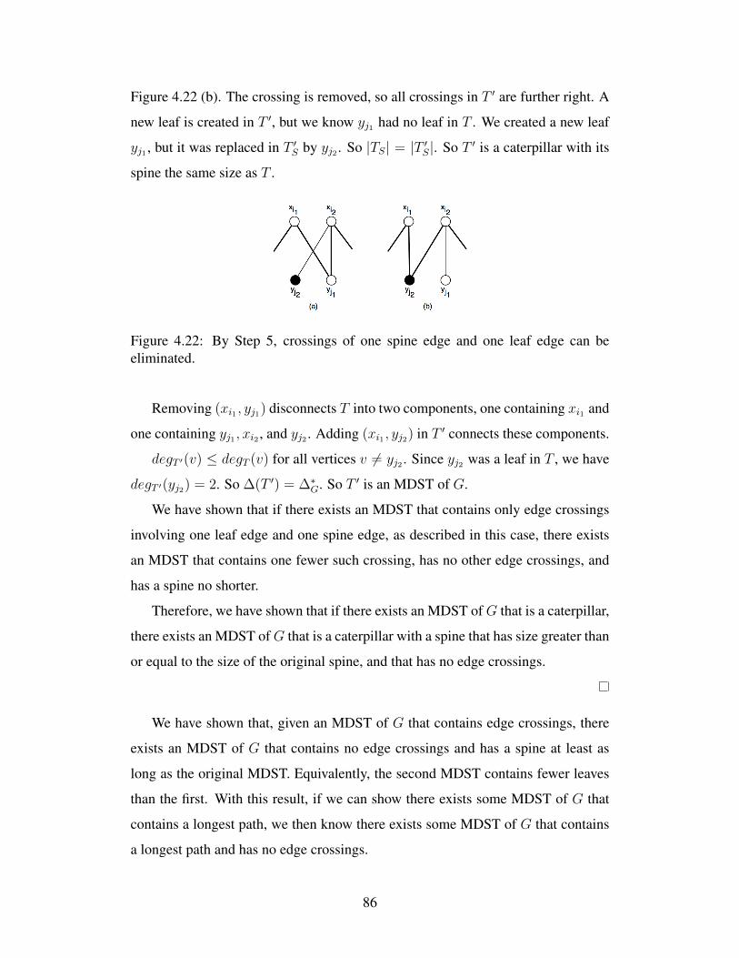
Figure 4.22 (b). The crossing is removed, so all crossings in T ′ are further right. A
new leaf is created in T ′, but we know yj1 had no leaf in T . We created a new leaf
yj1 , but it was replaced in T ′S by yj2 . So |TS| = |T ′S|. So T ′ is a caterpillar with its
spine the same size as T .
Figure 4.22: By Step 5, crossings of one spine edge and one leaf edge can beeliminated.
Removing (xi1 , yj1) disconnects T into two components, one containing xi1 and
one containing yj1 , xi2 , and yj2 . Adding (xi1 , yj2) in T ′ connects these components.
degT ′(v) ≤ degT (v) for all vertices v 6= yj2 . Since yj2 was a leaf in T , we have
degT ′(yj2) = 2. So ∆(T ′) = ∆∗G. So T ′ is an MDST of G.
We have shown that if there exists an MDST that contains only edge crossings
involving one leaf edge and one spine edge, as described in this case, there exists
an MDST that contains one fewer such crossing, has no other edge crossings, and
has a spine no shorter.
Therefore, we have shown that if there exists an MDST ofG that is a caterpillar,
there exists an MDST ofG that is a caterpillar with a spine that has size greater than
or equal to the size of the original spine, and that has no edge crossings.
We have shown that, given an MDST of G that contains edge crossings, there
exists an MDST of G that contains no edge crossings and has a spine at least as
long as the original MDST. Equivalently, the second MDST contains fewer leaves
than the first. With this result, if we can show there exists some MDST of G that
contains a longest path, we then know there exists some MDST of G that contains
a longest path and has no edge crossings.
86
Let G = (X, Y,E) be a strongly ordered, connected bipartite permutation
graph. Let P be the set of all zig-zag longest paths in G. Let T be a crossing-free
caterpillar MDST of G, and let P ∗ be the longest path in T that contains (x1, y1)
and (xp, yq). By Lemma 4.4, we know T contains these edges, and that they are
leaf edges on the endpoints of the spine of T . Therefore, such a P ∗ exists.
Lemma 4.21. Let G be a strongly ordered, connected bipartite permutation graph,
and let P ∗ be a zig-zag path inG that contains the edges (x1, y1) and (xp, yq). Then
the vertices in P ∗, V (P ∗), are contained in some zig-zag longest path in G.
Proof. If P ∗ itself is a longest path in G, then the lemma holds. Assume P ∗ is not
a longest path in G. Assume there does not exist a longest path in G that contains
V (P ∗). By Lemma 4.4 we know there exists some longest path in G that contains
the edges (x1, y1) and (xp, yq). Let P be the set of all such longest paths. Fix P ∈ P
such that the number of consecutive vertices of P ∗ that are in P starting from the
left is as large as possible. That is, choose P such that the first vertex in P ∗ − P is
positioned as far right in P ∗ as possible.
Assume without loss of generality that x ∈ X(P ∗) is the leftmost (in P ∗) vertex
in P ∗ − P . We know x is not an endpoint, or adjacent to an endpoint, in either P
or P ∗, since the edges (x1, y1) and (xp, yq) are in both paths. Fix yj1 , yj2 to be the
neighbours of x in P ∗ with yj1 < yj2 . By Lemma 4.7 we have yj1 , yj2 ∈ P .
Now consider the (yj1 , yj2)-subpath of P . Let Q be this subpath.
Case 1: There exists some x′ in Q such that x′ ∈ P − P ∗ or x < x′. In this
case, we will show how to build another zig-zag longest path P ′ that matches P ∗
up to some vertex further right than x.
If Q = yj1 , x′, yj2 , let P ′ = (V (P ), E(P ) − {(x′, yj1), (x′, yj2)} ∪ {(x, yj1),
(x, yj2)}). Now P ′ is a zig-zag longest path that contains the vertices of P ∗ from
the left up to yj2 instead of just to yj1 , a contradiction.
Now consider when |Q| > 3. Fix xi1 , xi2 such that Q = yj1 , xi1 , ..., xi2 , yj2 .
Let y′, y′′, y′ < y′′, be the neighbours of x′ in P . By the adjacency property,
Y (Q) ⊆ NG(x). Let P ′ = (V (P ), E(P )− {(x′, y′), (x′, y′′)} ∪ {(x, y′), (x, y′′)}).
We now have P ′ as a longest path that contains V (P ∗) further right than P . We
87
may have introduced edge crossings in P ′, but we know there exists a crossing-free
path containing the same vertices as P ′, since G is a bipartite permutation graph,
any subgraph of a bipartite permutation graph is also a bipartite permutation graph,
and P ′ is a Hamiltonian path in the bipartite permutation subgraph of G induced
by its vertices. Now we have a zig-zag longest path that contains the vertices of P ∗
from the left up to yj2 instead of just to yj1 . If x′ ∈ P ∗, we have x < x′, and so now
x′ could be the leftmost vertex in P ∗ − P , a contradiction.
Case 2: X(Q) ∈ P ∗ and X(Q) ≤ x. In this case, we want to find some x′ such
that x′ < x and x′ ∈ P − P ∗ and build a new path P ′ that contains x instead of x′.
First, we show that in this case, there must exist x′ ∈ P − P ∗. Since we have
assumed that P ∗ is not contained in any longest path ofG, then ∆∗G ≥ 3. By Lemma
4.14, we can assume that zig-zag longest paths in G all start in X or all start in Y .
Assume that there does not exist such an x′ (that is, all X vertices in P that are to
the left of x are also in P ∗), and consider the left endpoint of P .
Subcase 2a: Assume P starts in X . By our choice of P, then P starts at x1.
Since G is bipartite, the (x1, yj2)-subpath of P has even size. Let k be the number
of vertices in X in this subpath. Then there are also k vertices in Y in this subpath.
Then |P | = 2k + |back(P, yj2)|.
The (v1, yj2)-subpath of P ∗, where v1 = x1 or y1, contains x and so has one
more vertex in X than the subpath in P . Since yj2 ∈ Y is an endpoint of this
subpath, it must contain at least one more vertex in Y than P .
We also have that front(P ∗, yj2) ∩ back(P, yj2) = ∅, otherwise we would have
Case 1. Let P ′ = front(P ∗, yj2) ∪ {yj2} ∪ back(P, yj2). Now |P ′| = 2(k + 1) +
|back(P, yj2)| > |P |. We said P was a longest path, so this gives a contradiction.
Subcase 2b: Assume P starts in Y . By our choice of P, then P starts at y1.
Since G is bipartite, the (y1, yj2)-subpath of P has an odd number of vertices. Let
k be the number of vertices in X in this subpath. Then there are also k + 1 vertices
in Y in this subpath. Then |P | = 2k + 1 + |back(P, yj2)|.
The (v1, yj2)-subpath of P ∗, where v1 = x1 or y1, contains x and so has one
more vertex in X than the subpath in P . Since yj2 ∈ Y is an endpoint of this
subpath, it must contain at least one more vertex in Y than P .
88
We also have that front(P ∗, yj2) ∩ back(P, yj2) = ∅, otherwise we would have
Case 1. Let P ′ = front(P ∗, yj2) ∪ {yj2} ∪ back(P, yj2). Now |P ′| = 2(k + 1) +
|back(P, yj2)| > |P |. We said P was a longest path, so this gives a contradiction.
Therefore, there exists some x′ ∈ P−P ∗ with x′ < x. Fix x′ to be the rightmost
such vertex and let y′ be the leftmost neighbour of x′ in P . We will now show how
to construct another zig-zag longest path P ′ that contains the vertices of P ∗ further
right than P .
Let Xr = xr0 , xr1 , ..., xri with rj < rj+1 be the vertices in X(P ) between x′
and x, where xr0 = x′, and x /∈ Xr. Let Yr = yr0 , yr1 , ..., yri+1be the neighbours
of XP in P such that the leftmost neighbour of xrj in P is yrj and the rightmost
neighbour of xrj in P is yrj+1. Let yr0 = y′ and yri+1
= yj2 . By our choices of x
and x′, we know that all vertices in P ∗ between x′ and x, and between y′ and yj2
are in XP ∪ YP .
Constructing P ′ requires that we show (xrj , yrj−1) ∈ E(G) for 1 ≤ j ≤ i.
Define left(v, P ) to be the leftmost neighbour of v in zig-zag path P and define
right(v, P ) to be the rightmost neighbour in zig-zag path P . Since G is a bipartite
permutation graph and has the adjacency property, we can show these edge are in
E(G) by showing that left(v, P ∗) < left(v, P ) for all v ∈ XP .
First consider xri . Since xri is on the (yj1 , yj2)-subpath in P , we have left(xri , P )
≥ yj1 . We have that yj1 = left(x, P ∗), and since xri < x, and our paths are zig-
zags, then left(xri , P∗) < yj1 ≤ left(xri , P ).
Next, for the rest ofXr, we know that for xrj and xrk with xrj <xrk , left(xrj , P )
= yrj < left(xrk , P ) = yrk and there are exactly as many vertices in Xr between
xrj and xrk as there are between yrj and yrk in Yr. Now consider left(xrj , P∗)
and left(xrk , P∗). Moving from right to left, we know that the distance between
left(xrj , P ) and left(xrk , P ) is the same as the distance between xrj and xrk . How-
ever, since V (P ∗) ⊂ V (P ) in this subpath, but Yr is not necessarily contained in
P ∗, then the distance between left(xrj , P∗) and left(xrk , P
∗) is at least the dis-
tance between xrj and xrk . Therefore, since we already had that left(xri , P∗) <
left(xri , P ), for each xrj ∈ Xr, we have that left(xrj , P∗) < yj1 ≤ left(xrj , P ).
So (xrj , yrj−1) ∈ E(G) for 1 ≤ j ≤ i.
89
Let EL = {(xrj , yrj−1)}, for 1 ≤ j ≤ i, and let ER = {(xrj , yrj+1
)} for 1 ≤
j ≤ i.
Now, let P ′ = (V (P ), E(P )− {ER, (x′, y′), (x′, right(x′, P ))} ∪ {EL, (x, yri),
(x, yj2)}). The edges between each xrj and its rightmost neighbour in P are re-
moved, as well as the edges containing x′. The edges added in EL connect each xrjto the vertex in Y (P ) immediately left of its leftmost neighbour. We showed above
that these edges are in G. This results in two subpaths, one from the left up to yri ,
which is now right(xri , P′), and the other beginning at yj2 and going to the right.
We know (x, yj2) ∈ E(G) because it is in P ∗. We also know that yri ≥ yj1 . By
the adjacency property, (x, yri) ∈ E(G). Adding these edges connects the two path
components. Therefore P ′ is a path.
Each edge added between xrj and yrj−1will not introduce any edge crossings
because the only edge in P it would cross is (xrj−1, yrj), which is in ER. Therefore,
P ′ contains no edge crossings and is a zig-zag.
P ′ contains all vertices of P except for x′, and it instead contains x. Therefore,
P ′ is a zig-zag longest path that contains the vertices of P ∗ further to the right than
P , a contradiction.
Therefore, there must exist a zig-zag longest path in G that contains the vertices
of P ∗.
Theorem 4.22. Let G = (X, Y,E) be a strongly ordered, connected bipartite per-
mutation graph. Then there exists a crossing-free caterpillar MDST of G that con-
tains a longest path of G.
Proof. Assume that no MDST of G contains a longest path. That is, for every
MDST T of G, the longest path P ∗ in T has size less than the size of a longest path.
Choose T to be a crossing-free MDST of G and let P ∗ be the spine of T .
By Lemma 4.21, there is some longest path that contains the vertices of P ∗. Fix
P to be such a zig-zag longest path. Let E ′ be the set of edges in T that contain a
vertex in V (P ).
Let T ′ = (V (T ), E(T )− E ′ ∪ E(P ). First, we show that T ′ is a spanning tree.
The subgraph of T induced by E ′ contains the spine of T and some leaves. Since
90
V (P ∗) ⊂ V (P ), this subgraph contains only spine vertices and leaves in T that are
also on P . If a vertex is not in E ′, then it is not in P . Therefore, |E ′| = |P | − 1.
Since P is a path, |E(P )| = |P |−1 as well, and so T ′ contains the same number of
edges as T . Removing the edges of E ′ from T produces components that are either
isolated vertices, which were either leaves in T that were on P , or spine vertices
in T that were only adjacent to other vertices that were in P , or are K2, containing
one vertex from P ∗ and another vertex from T −P . Since each component contains
exactly one vertex from P , adding the edges from P connects the tree.
Now consider the degrees of vertices in T ′. For all vertices in T −P , the degree
remained the same. Vertices in P − P ∗ were leaves in T and are on the spine of
T ′. However, since we removed the one edge containing these vertices from T and
only added path edges back, vertices in P − P ∗ will have degree at most 2 in T .
Vertices in P ∗ have degree at least 2 in T . In T ′, some of these vertices will
have leaves removed, if these leaves were in P − P ∗. Then, each vertex in P ∗ has
its two incident spine edges removed, and replaced with two path edges from P .
Therefore, degT ′(v) ≤ degT (v), for all v ∈ P ∗. Therefore, T ′ is an MDST of G.
It is possible that edge crossings were introduced in the construction of T ′. If
T ′ contains edge crossings, by Theorem 4.20, there exists another MDST of G that
contains no edge crossings and has a spine at least as long as T ′. Since T ′ contains
a longest path, this other MDST will also contain a longest path.
Therefore, by contradiction, there exists a crossing-free MDST of G that con-
tains a longest path.
4.4 An Algorithm for ∆∗G of a Bipartite PermutationGraph
We now present a dynamic programming algorithm to solve the minimum degree
spanning tree problem on and construct an MDST of a bipartite permutation graph.
Let G = (X, Y,E) be a connected bipartite permutation graph with strong or-
dering x1, ..., xp, y1, ..., yq. We define [i, j] to be the induced subgraph of G con-
91
taining the vertices xi, ..., xp, yj, ..., yq.
Lemma 4.23. Let G = (X, Y,E) be a connected bipartite permutation graph with
strong ordering x1, ..., xp, y1, ..., yq, and for all 1 ≤ i ≤ p, 1 ≤ j ≤ q, let
∆∗x[i, j] =
∞ if [i, j] is not connected∆([i, j]) if [i, j] is a tree with xi as a leaf∞ if N[i,j](yj) = {xi}mink{max{k + 1,∆∗y[i+ k, j]}} for 1 ≤ k ≤ |N[i,j](yj)| − 1 otherwise
and
∆∗y[i, j] =
∞ if [i, j] is not connected∆([i, j]) if [i, j] is a tree with yj as a leaf∞ if N[i,j](xi) = {yj}mink{max{k + 1,∆∗x[i, j + k]}} for 1 ≤ k ≤ |N[i,j](xi)| − 1 otherwise
Then for all i, j, (1) ∆∗x[i, j] is the minimum maximum degree of a crossing-free
spanning tree of [i, j] with xi as a leaf, and (2) ∆∗y[i, j] is the minimum maximum
degree of a crossing-free spanning tree of [i, j] with yj as a leaf.
Proof. Let i = p and j = q. By Theorem 4.2, the edge (xp, yq) is in every bipartite
permutation graph. Therefore, the subgraph [p, q] consists of just that edge, which
is a tree with both xp and yq as leaves. So ∆∗x[p, q] = ∆([p, q]) = 1 and ∆∗y[p, q] =
∆([p, q]) = 1.
Assume the claim holds for all [i, j] such that i > a and j ≥ b, or i ≥ a and
j > b.
Now consider ∆∗x[a, b]. If [a, b] is not connected, then it does not have a spanning
tree, and ∆∗[a,b] = ∆∗x[a, b] = ∞. If [a, b] is a tree with xa as a leaf, then there is
exactly one spanning tree of [a, b], and by Theorem 4.16, we know it is crossing-
free. Thus, in this case ∆∗x[a, b] = ∆([a, b]). If [a, b] is a tree without xa as a leaf,
then N[a,b](yb) = xa. If N[a,b](yb) = xa, there is no crossing-free spanning tree of
[a, b] with xa as a leaf, since in this case any crossing-free spanning tree must have
yb as a leaf of xa. Thus, in this case ∆∗x[a, b] =∞.
92
In all other cases, we claim that ∆∗x[a, b] = mink{max{k + 1,∆∗y[a + k, b]}}
for 1 ≤ k ≤ |N[a,b](yb)| − 1. In all crossing-free spanning trees of [a, b] with xa
as a leaf, xa must be a leaf of yb, and yb can have between one and |N[a,b](yb)| − 1
leaves in such a crossing-free spanning tree, plus one non-leaf (spine) neighbour.
Thus, the degree of yb in a crossing-free spanning tree of [a, b] is k + 1 where k is
the number of leaves of yb.
Let ∆′x be the minimum maximum degree of a crossing-free spanning tree of
[a, b] with xa as a leaf. First, assume ∆′x > ∆∗x[a, b]. Then all crossing-free spanning
trees of [a, b] with xa as a leaf must have maximum degree ≥ ∆′x. Let l be the
value of k that minimizes max{k + 1,∆∗y[a + k, b]}. So ∆′x > l + 1 and ∆′x >
∆∗y[a + l, b]. Let Ty be a crossing-free MDST of [a + l, b]. Let T = (V (Ty) ∪
{xa, ..., xa+l−1}, E(Ty) ∪ {(x′, yb) |xa ≤ x′ ≤ xa+l−1}). Now T is a crossing-free
spanning tree of [a, b] with xa as a leaf and ∆(T ) = max{l+ 1,∆∗y[a+ l, b]} < ∆′x,
a contradiction.
Now assume ∆′x < ∆∗x[a, b]. Let T be a crossing-free spanning tree of G with
xa as a leaf, such that ∆(T ) = ∆′x. Since T is crossing-free, yb has between one and
|N[a,b](yb)|−1 leaves in T . Let l be the number of leaves yb has in T . Then ∆(T ) ≥
l+1. Since ∆∗x[a, b] is too large, then when k = l, we must have ∆∗y[a+l, b] > ∆′x ≥
l + 1. Let Ty = (V (T ) − {xa, ..., xa+l−1}, E(T ) − {(x′, yb) |xa ≤ x′ ≤ xa+l−1}).
Now Ty is a crossing-free spanning tree of [a+l, b] with yb as leaf, and ∆(Ty) ≤ ∆′x.
Therefore, ∆(Ty) < ∆∗y[a + l, b]. But by our inductive hypothesis, ∆∗y[a + l, b] is
the minimum maximum degree of a crossing-free spanning tree of [a+ l, b] with yb
as a leaf, a contradiction. Therefore, ∆′x = ∆∗x[a, b].
Therefore, (1) holds. An equivalent argument can be made for (2), and so the
lemma holds.
Theorem 4.24. For a strongly ordered, connected bipartite permutation graph G,
∆∗G can be found in O(n3) time.
Proof. By Corollary 4.19, every crossing-free spanning tree of a bipartite permu-
tation graph is a caterpillar. By Lemma 4.17, if [i, j] is connected then the edge
93
(xi, yj) is in any crossing-free spanning tree of [i, j]. If G has two or fewer vertices,
then eitherG has no edges orG has at most one edge and that edge is a crossing-free
spanning tree of G. We now assume that G contains at least three vertices.
If both xi and yj are in the spine, then they each have a leaf, y′ and x′ respec-
tively such that xi < x′ and yj < y′. Then (xi, y′), (x′, yj) is an edge crossing.
Therefore, at least one of xi, yj must be a leaf. By the definition of a caterpillar,
leaf vertices are only adjacent to spine vertices so at most one of xi, yj is a leaf
vertex.
Therefore, in any crossing-free spanning tree, either xi is a leaf or yj is a leaf.
Then the minimum maximum degree of crossing-free spanning trees of [i, j] can
be expressed as the minimum of the minimum maximum degree of crossing-free
spanning trees of [i, j] with xi as a leaf and the minimum maximum degree of
crossing-free spanning trees of [i, j] with yj as a leaf.
By Lemma 4.23, we know that ∆∗x[i, j] is the minimum maximum degree of a
crossing-free spanning tree of [i, j] with xi as a leaf, and ∆∗y[i, j] is the minimum
maximum degree of a crossing-free spanning tree of [i, j] with yj as a leaf. There-
fore, min{∆∗x[i, j],∆∗y[i, j]} gives the minimum maximum degree of a crossing-free
spanning tree of G. By Theorem 4.18 there exists an MDST of all bipartite permu-
tation graphs that is crossing free, and so ∆∗[i,j] = min{∆∗x[i, j],∆∗y[i, j]}.
When i = 1, j = 1, then [i, j] = G. Therefore, ∆∗G = min{∆∗x[1, 1],∆∗y[1, 1]}
for a bipartite permutation graph G.
An algorithm based on the formulas of the lemma constructs two p by q tables
for ∆∗x[i, j] and ∆∗y[i, j], for a total of 2 × p × q ∈ O(n2) entries. For each entry,
k ≤ max{p, q} ≤ n. Thus, the algorithm finds ∆∗G in O(n3) time.
Theorem 4.25. For a strongly ordered, connected bipartite permutation graph G,
an MDST of G can be constructed in O(n3) time.
Proof. Using the tables produced by the algorithm, we can construct a crossing-
free spanning tree T of each [i, j] where ∆∗x[i, j] is finite such that xi is a leaf in T
and ∆(T ) = ∆∗x[i, j]. If [i, j] is a tree, then [i, j] is a crossing-free spanning tree
94
of itself. Otherwise, we can construct T by choosing a value of k that minimizes
max{k+ 1,∆∗y[i+ k, j]} and adding xi, ..., xi+k−1 as leaves of yj to a crossing-free
spanning tree T ′ of [i+ k, j] with ∆(T ′) = ∆∗y[i+ k, j] that has yj as a leaf.
Similarly, we can construct a crossing-free spanning tree T of each [i, j] where
∆∗y[i, j] is finite such that yj is a leaf in T and ∆(T ) = ∆∗y[i, j]. If [i, j] is a tree,
then [i, j] is a crossing-free spanning tree of itself. Otherwise, we can construct
T by choosing a value of k that minimizes max{k + 1,∆∗x[i, j + k]} and adding
yj, ..., yj+k−1 as leaves of xi to a crossing-free spanning tree T ′ of [i, j + k] with
∆(T ′) = ∆∗x[i, j + k] that has xi as a leaf.
By Theorem 4.24, we know ∆∗G = min{∆∗x[1, 1],∆∗y[1, 1]}, and so we can use
this method to construct a crossing-free MDST of G.
Therefore, the theorem holds.
95
Chapter 5
Conclusion
We now summarize the work presented in this thesis, and discuss some directions
for future work.
5.1 Summary
In this thesis, we explored the minimum degree spanning tree problem on bipartite
permutation graphs and their subclasses.
Chain graphs are a subclass of bipartite permutation graphs, and we give an
algorithm to construct an MDST on a given chain graph, as well as a formula to
find ∆∗G for a chain graph G in O(n2) time.
For bipartite permutation graphs, we build on work done on the Hamiltonian
path and longest path problems to get a number of structural results for longest
paths and MDSTs on this class. We show which vertices must be in a zig-zag
longest path in a bipartite permutation graph, and that certain longest paths can
only exist in a bipartite permutation graph with a Hamiltonian path.
We generalize the idea of zig-zag paths to show that every bipartite permutation
graph has an MDST that has no edge crossings, and so is a caterpillar. We also
show that every bipartite permutation graph has an MDST with no edge crossings
that contains a longest path.
We present a dynamic programming algorithm that solves the minimum degree
spanning tree problem for bipartite permutation graphs by finding ∆∗G and con-
structing an MDST of G in O(n3) time.
96
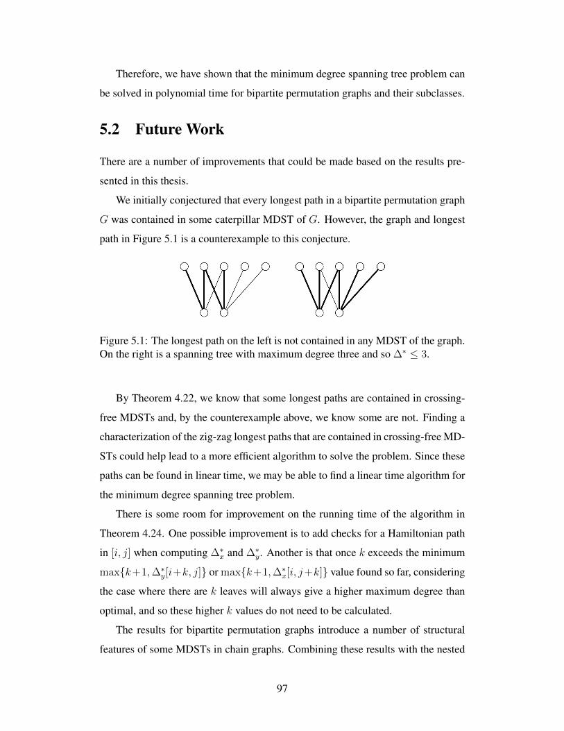
Therefore, we have shown that the minimum degree spanning tree problem can
be solved in polynomial time for bipartite permutation graphs and their subclasses.
5.2 Future Work
There are a number of improvements that could be made based on the results pre-
sented in this thesis.
We initially conjectured that every longest path in a bipartite permutation graph
G was contained in some caterpillar MDST of G. However, the graph and longest
path in Figure 5.1 is a counterexample to this conjecture.
Figure 5.1: The longest path on the left is not contained in any MDST of the graph.On the right is a spanning tree with maximum degree three and so ∆∗ ≤ 3.
By Theorem 4.22, we know that some longest paths are contained in crossing-
free MDSTs and, by the counterexample above, we know some are not. Finding a
characterization of the zig-zag longest paths that are contained in crossing-free MD-
STs could help lead to a more efficient algorithm to solve the problem. Since these
paths can be found in linear time, we may be able to find a linear time algorithm for
the minimum degree spanning tree problem.
There is some room for improvement on the running time of the algorithm in
Theorem 4.24. One possible improvement is to add checks for a Hamiltonian path
in [i, j] when computing ∆∗x and ∆∗y. Another is that once k exceeds the minimum
max{k+1,∆∗y[i+k, j]} or max{k+1,∆∗x[i, j+k]} value found so far, considering
the case where there are k leaves will always give a higher maximum degree than
optimal, and so these higher k values do not need to be calculated.
The results for bipartite permutation graphs introduce a number of structural
features of some MDSTs in chain graphs. Combining these results with the nested
97

neighbourhood properties of chain graphs, it may be possible to improve on our
result for finding an MDST in a chain graph. In particular, it is worth considering
the possibility that an MDST can be constructed for an arbitrary chain graph in
linear time.
The results in this thesis could also be generalized to superclasses of bipartite
permutation graphs. Biconvex graphs have an ordering that generalizes the strong
ordering of bipartite permutation graphs [1]. The properties of this ordering may
allow our results on bipartite permutation graphs to be generalized to this class of
graphs.
We use the nested neighbourhood ordering property of chain graphs in our al-
gorithm to solve the minimum degree spanning tree problem on these graphs. The
nested neighbourhood ordering also appears in the independent set in the partition
of a threshold graph, and so these results may be transferable to threshold graphs as
well.
In this thesis, we focus on the Hamiltonian path and longest path problems
as starting points to solve the minimum degree spanning tree problem. However,
there are other related problems that may also be helpful in solving this problem
on other graph classes. One potential area for exploration is the dominating path
problem. This problem can be solved in linear time on AT-free graphs [13]. A
dominating path can be used to easily construct a spanning caterpillar of a graph,
by adding all vertices not on the path as leaves. In a crossing-free MDST of a
bipartite permutation graph, the spine of the caterpillar is a dominating path in the
graph. It is worth exploring if a relationship exists between the dominating path
problem and the minimum degree spanning tree problem.
98
Bibliography
[1] N Abbas and L Stewart. Biconvex graphs: ordering and algorithms. DiscreteApplied Mathematics, 103(1-3):1–19, 2000.
[2] L Babel and G Woeginger. Pseudo-Hamiltonian graphs. In Proceedings ofthe 23rd International Workshop on Graph-Theoretic Concepts in ComputerScience (WG’97), volume 1335 of LNCS, pages 38–51. Springer-Verlag, 1997.
[3] H Bodlaender, T Kloks, and D Kratsch. Treewidth and pathwidth of permu-tation graphs. In Automata, Languages and Programming, volume 700 ofLNCS, pages 114–125. Springer Berlin / Heidelberg, 1993.
[4] J A Bondy and V Chvatal. A method in graph theory. Discrete Mathematics,15(2):111 – 135, 1976.
[5] O Boruvka. On a minimal problem. Prace Moravske Pridovedecke Spolec-nosti, 3, 1926.
[6] A Brandstadt and D Kratsch. On the restriction of some NP-complete graphproblems to permutation graphs. In L Budach, editor, Fundamentals of Com-putation Theory, volume 199 of LNCS, pages 53–62. Springer Berlin / Hei-delberg, 1985.
[7] A Brandstadt, V.B. Le, and J. Spinrad. Graph classes: a survey. Society forIndustrial and Applied Mathematics, Philadelphia, PA, USA, 1999.
[8] Y Caro, I Krasikov, and Y Roditty. On the largest tree of given maximumdegree in a connected graph. Journal of Graph Theory, 15(1):7–13, 1991.
[9] K Chaudhuri, S Rao, S Riesenfeld, and K Talwar. What would Edmonds do?Augmenting paths and witnesses for degree-bounded MSTs. Algorithmica,55(1):157–189, 2009.
[10] B Chazelle. A minimum spanning tree algorithm with inverse-Ackermanntype complexity. Journal of the ACM, 47(6):1028–1047, 2000.
[11] V Chvatal and P Erdos. A note on Hamiltonian circuits. Discrete Mathemat-ics, 2(11):1–1, 1972.
[12] T Cormen, C Leiserson, R Rivest, and C Stein. Introduction to Algorithms.The MIT Press, New York, second edition, 2001.
[13] D Corneil, S Olariu, and L Stewart. A linear time algorithm to compute a dom-inating path in an AT-free graph. Information Processing Letters, 54(5):253–257, 1995.
99
[14] D Corneil, S Olariu, and L Stewart. Asteroidal triple-free graphs. SIAMJournal of Discrete Mathematics, 10(3):399–430, 1997.
[15] A Czumaj and WB Strothmann. Bounded degree spanning trees. In R Burkardand G Woeginger, editors, Algorithms ESA ’97, volume 1284 of LNCS, pages104–117. Springer Berlin / Heidelberg, 1997.
[16] A Czygrinow, G Fan, G Hurlbert, HA Kierstead, and WT Trotter. Spanningtrees of bounded degree. The Electronic Journal of Combinatorics, 8(R33):1,2001.
[17] P Damaschke, JS Deogun, D Kratsch, and G Steiner. Finding Hamiltonianpaths in cocomparability graphs using the bump number algorithm. Order,8:383–391, 1992.
[18] EW Dijkstra. A note on two problems in connexion with graphs. Numerischemathematik, 1(1):269–271, 1959.
[19] GA Dirac. Some theorems on abstract graphs. Proceedings of the LondonMathematical Society, 3(1):69, 1952.
[20] P Eades, B McKay, and N Wormald. On an edge crossing problem. In Pro-ceedings of the Ninth Australian Computer Science Conference. 1986.
[21] S Fekete, S Khuller, M Klemmstein, and B Raghavachari. A network-flowtechnique for finding low-weight bounded-degree spanning trees. Journal ofAlgorithms, 24:310–324, 1997.
[22] H Fernau, J Kneis, D Kratsch, A Langer, M Liedloff, D Raible, and P Ross-manith. An exact algorithm for the maximum leaf spanning tree problem. InJ Chen and F Fomin, editors, Parameterized and Exact Computation, volume5917 of LNCS, pages 161–172. Springer Berlin / Heidelberg, 2009.
[23] T Fischer. Optimizing the degree of minimum weight spanning trees. Tech-nical Report 93-1338, Department of Computer Science, Cornell University,1993.
[24] M Furer and B Raghavachari. An NC approximation algorithm for the min-imum degree spanning tree problem. Proceedings of the 28th Annual Aller-ton Conference on Communication, Control and Computing, pages 274–281,1990.
[25] M Furer and B Raghavachari. Approximating the minimum-degree Steinertree to within one of optimal. Journal of Algorithms, 17(3):409–423, 1994.
[26] H.N Gabow and R.E Tarjan. Efficient algorithms for a family of matroidintersection problems. Journal of Algorithms, 5(1):80–131, 1984.
[27] MR Garey and DS Johnson. Computers and intractability. A guide to thetheory of NP-completeness. W. H. Freeman & Co., New York, 1979.
[28] MX Goemans. Minimum bounded degree spanning trees. 47th Annual IEEESymposium on Foundations of Computer Science, 2006. FOCS’06, pages 273–282, 2006.
100
[29] MC Golumbic. Algorithmic Graph Theory and Perfect Graphs (Annals ofDiscrete Mathematics, Vol 57). North-Holland, Amsterdam, The Netherlands,second edition, 2004.
[30] RL Graham and P Hell. On the history of the minimum spanning tree problem.Annals of the History of Computing, 7(1):43–57, 1985.
[31] F Harary and U Peled. Hamiltonian threshold graphs. Discrete Applied Math-ematics, 16(1):15, 1987.
[32] K Ioannidou, G Mertzios, and S Nikolopoulos. The longest path problem ispolynomial on interval graphs. In R Krlovic and D Niwinski, editors, Mathe-matical Foundations of Computer Science 2009, volume 5734 of LNCS, pages403–414. Springer Berlin / Heidelberg, 2009.
[33] V Jarnık. About a certain minimal problem. Prace Moravske PridovedeckeSpolecnosti, 6:57–63, 1930.
[34] R Jothi and B Raghavachari. Degree-bounded minimum spanning trees. Dis-crete Applied Mathematics, 157(5):960–970, 2009.
[35] JB Kruskal Jr. On the shortest spanning subtree of a graph and the travel-ing salesman problem. Proceedings of the American Mathematical society,7(1):48–50, 1956.
[36] J M Keil. Finding Hamiltonian circuits in interval graphs. Information Pro-cessing Letters, 20(4):201–206, 1985.
[37] S Khuller, B Raghavachari, and N Young. Low degree spanning trees of smallweight. Proceedings of the twenty-sixth annual ACM symposium on Theoryof computing, page 421, 1994.
[38] H Kishimoto and M Kano. Spanning k-trees of n-connected graphs. Graphsand Combinatorics, pages 1–6, 2011.
[39] E.L Lawler. Combinatorial Optimization: Networks and Matroids. Holt,Rinehart, and Winston, New York, 1976.
[40] GB Mertzios and DG Corneil. A simple polynomial algorithm for thelongest path problem on cocomparability graphs. Technical report availableat http://arxiv.org/abs/1004.4560, 2010.
[41] J Moon and L Moser. On Hamiltonian bipartite graphs. Israel Journal ofMathematics, 1(3):163–165, 1963.
[42] H Muller. Hamiltonian circuits in chordal bipartite graphs. Discrete Mathe-matics, 156(1):291–298, 1996.
[43] V Neumann-Lara and E Rivera-Campo. Spanning trees with bounded degrees.Combinatorica, 11(1):55–61, 1991.
[44] O Ore. Note on Hamilton circuits. American Mathematical Monthly,67(1):55–55, 1960.
[45] K Ozeki and T Yamashita. Spanning trees: A survey. Graphs and Combina-torics, pages 1–26, 2010.
101
[46] RC Prim. Shortest connection networks and some generalizations. Bell systemtechnical journal, 36(6):1389–1401, 1957.
[47] R Ravi and M Singh. Delegate and conquer: An LP-based approximation al-gorithm for minimum degree MSTs. In M Bugliesi, B Preneel, V Sassone, andI Wegener, editors, Automata, Languages and Programming, volume 4051 ofLNCS, pages 169–180. Springer Berlin / Heidelberg, 2006.
[48] SJ Riesenfeld. Optimization and reconstruction over graphs. PhD. thesis,University of California at Berkeley, Jan 2008.
[49] G Robins and JS Salowe. Low-degree minimum spanning trees. Discrete andComputational Geometry, 14(1):151–165, 1995.
[50] M Singh and LC Lau. Approximating minimum bounded degree spanningtrees to within one of optimal. Proceedings of the thirty-ninth annual ACMsymposium on Theory of computing, page 670, 2007.
[51] J Spinrad, A Brandstadt, and L Stewart. Bipartite permutation graphs. Dis-crete Applied Mathematics, 18(3):279–292, 1987.
[52] R Uehara and Y Uno. On computing longest paths in small graph classes.International Journal of Foundations of Computer Science, 18(5):911–930,2007.
[53] R Uehara and G Valiente. Linear structure of bipartite permutation graphsand the longest path problem. Information Processing Letters, 103(2):71–77,2007.
[54] D West. Introduction to Graph Theory. Prentice Hall, second edition, 2000.
[55] S Win. On a conjecture of Las Vergnas concerning certain spanning trees ofgraphs. Resultate der Mathematik, 2:215–224.
[56] S Win. Uber Geruste mit vorgeschriebenen Maximalgraden und eine Vermu-tung von Las Vergnas. Ph.D. Thesis, Universitat Hamburg, 1979.
[57] S Win. On a connection between the existence of k-trees and the toughness ofa graph. Graphs and Combinatorics, 5(1):201–205, 1989.
[58] M Yannakakis. The complexity of the partial order dimension problem. SIAMJournal on Algebraic and Discrete Methods, 3(3):351–358, 1982.
[59] L Zhenhong and X Baoguang. On low bound of degree sequences of spanningtrees in k-edge-connected graphs. Journal of Graph Theory, 28(2):87–95,1998.
102