J. Biomedical Science and Engineering, 2014, 7, 721-730 Published Online July 2014 in SciRes. http://www.scirp.org/journal/jbise http://dx.doi.org/10.4236/jbise.2014.79071

How to cite this paper: Kengne, E., et al. (2014) A Mathematical Model to Solve Bio-Heat Transfer Problems through a Bio- Heat Transfer Equation with Quadratic Temperature-Dependent Blood Perfusion under a Constant Spatial Heating on Skin Surface. J. Biomedical Science and Engineering, 7, 721-730. http://dx.doi.org/10.4236/jbise.2014.79071

A Mathematical Model to Solve Bio-Heat Transfer Problems through a Bio-Heat Transfer Equation with Quadratic Temperature-Dependent Blood Perfusion under a Constant Spatial Heating on Skin Surface Emmanuel Kengne*, Idir Mellal, Mariem Ben Hamouda, Ahmed Lakhssassi Department of Computer Science and Engineering, University of Quebec at Outaouais, Gatineau, Canada Email: *kengem01@uqo.ca, idir.mellal@gmail.com, mariembh02@gmail.com, ahmed.Lakhssassi@uqo.ca Received 22 May 2014; revised 6 July 2014; accepted 16 July 2014

Copyright © 2014 by authors and Scientific Research Publishing Inc. This work is licensed under the Creative Commons Attribution International License (CC BY). http://creativecommons.org/licenses/by/4.0/

Abstract We consider the one-dimensional bio-heat transfer equation with quadratic temperature-depen- dent blood perfusion, which governs the temperature distribution inside biological tissues. Using an extended mapping method with symbolic computation, we obtain the exact analytical thermal traveling wave solution, which describes the non-uniform temperature distribution inside the bodies. The found exact solution is used to investigate the temperature distribution in the tissues. It is found that the surrounding medium with higher temperature does not necessarily imply that the tissue will quickly (after a short duration of heating process) reach the desired temperature. It is also found that increased perfusion causes a decline in local temperature.

Keywords Bio-Heat Transfer Problems, Pennes Bio-Heat Model, Temperature-Dependent Blood Perfusion, Thermal Therapy, Extended Mapping Method

1. Introduction Using the Pennes bio-heat transfer (BHT) equation [1] which accounts for the ability of tissue to remove heat by

*Corresponding author.

E. Kengne et al.

722

both passive conduction and perfusion of tissue by blood, many of the bio-heat transfer problems have been modelled. The BHT equation defines the thermal behavior of tissue and includes four terms that influence the heat transfer at the tissue surface: the heat exchange between the tissue surface and the environment, the conduction through the tissue, the energy transfer by blood circulation in the tissue, and the heat generation due to local metabolism. The contributions of heat conduction and perfusion are combined in the Pennes bio-heat equation [1] [2], that we use in a form that employs mω [3]

( ) ( )[ ] , , 0.b b m a m rTc k T c T T T Q Q x tt

ρ ρ ω∂= ∇ ⋅ ∇ − − + + ∈Ω >

∂ (1.1)

Here, ρ , c and k are the density, specific heat, and thermal conductivity of tissue, respectively, bc is the specific heat of blood, bρ is the density of blood, T is local tissue temperature, aT is the arterial blood temperature, t is the time, mQ is the metabolic heat generation rate per unit volume, rQ is the heat depo- sited per volume due to spatially distributed heating, and mω is the blood perfusion rate. The BHT model (1.1) can be used for the quantitative diagnostics of physiological conditions on biological bodies, as for example, for simulations of regional hyperthermia for cancer therapy [3]-[5]. For thermal problems, Equation (1.1) is subject to the usual boundary conditions 1) temperature prescribed, ( )boundaryT T= , where (boundary) is either the

whole or a part of the boundary of domain Ω ; or 2) heat flux prescribed, q q= ; or 3) convection,

( )( )surrboundaryfq h T T= − − , where fh is the heat transfer coefficient and surrT is the temperature of the

surrounding medium; or radiation, ( )( )4 4

am boundaryq T Tσε= − − , where σ is the Stefan-Boltzman constant, ε

is the radiative interchange factor between the surface and the exterior ambient temperature amT . The parameters considered in Equation (1.1) are usually assumed to be constant except for the blood

perfusion, which varies with temperature T to include the specific case of temperature-dependent perfusion [3]-[5]. Perfusion is defined as the nonvectorial volumetric blood flow per tissue volume in a region that contains sufficient capillaries that an average flow description is considered reasonable. Therefore it is expected that the heat dissipation should vary with the blood perfusion rate. Most tissues, including much of the skin and brain, are highly perfused, with a perfusion coefficient denoted by ω , can be replaced, as in Equation (1.1), by

mω , the nondirectional mass flow associated with perfusion. One of the most important applications of blood perfusion effects and measurements is tumour detection. Tumours are known to have a different perfusion rate than normal healthy tissue. They are generally highly vascular and so blood flows through them more quickly. Therefore the ability to know the effects and the measurements of this abnormal perfusion rate could help evaluate the size and severity of a tumour. By varying some parameters of the blood perfusion ( )m Tω , it is possible to examine the effect that different volume flow rates of blood have on the heat transfer inside the biological bodies.

The analytical study of Equation (1.1) as a nonlinear evolution equation is of great interest. As in the study of nonlinear physical phenomena, the investigations of the travelling wave solution of Equation (1.1) play an im- portant role in the analytical study of the nonuniform thermal distribution in biological tissues. The importance of obtaining the analytical solutions, if available, of Equation facilitates 1) the investigation of temperature distribution inside the biological bodies, 2) the verification of numerical solvers, and aids in the stability analysis of solutions. In the present work, we aim to find analytical thermal traveling wave solution of one-dimensional (1D) BHT equation

( )[ ]2

2 , , 0,b b m a m rT Tc k c T T T Q Q x tt x

ρ ρ ω∂ ∂= − − + + ∈Ω >

∂ ∂ (1.2)

with a quadratic temperature-dependent blood perfusion [6]-[8] 2

0 0 0 0, 0,m T Tω ω γ δ δ= + + ≠ (1.3)

where 0 0ω > is the baseline perfusion, 0 0γ > and 0 0δ > are respectively the linear and quadratic coeffi- cients of temperature-dependence. Here, we assume that the skin surface is defined at 0x = while the body core at x L= so that [ ]0, LΩ = . For the simplicity, we will limit ourselves to the special case of constant spatial heating. This reflects the situation where the human skin was heated by a laser [9] [10]. The analytical

E. Kengne et al.

723

solutions will allow us to investigate the effect of the blood perfusion on heat transfer in the tissues. The analytical solutions are obtained with the help of the extended mapping method [11] [12]. The rest of the work is organized as follows. In Section 2, we present analytical thermal traveling wave solution of Equation (1.2) with blood perfusion (1.3). The results are discussed in Section 3. In Section 4, we conclude our work by summa- rizing the main results.

2. Thermal Traveling Wave Solutions of the 1D BHT Model with Quadratic Temperature-Dependent Blood Perfusion

In this section, we aim to apply the extended mapping method to find analytical solutions of Equation (1.1) with quadratic temperature-dependent blood perfusion (1.3). For the traveling wave solutions of Equations (1.2), (1.3), we introduce the ansatz

( ) ( ), ,T x t u z ax tυ= = − (1.4)

where a and υ are two real parameters be determined later. Inserting ansatz (1.4) into Equations (1.2), (1.3) yields the ordinary differential equation (ODE)

( ) ( )2

2 3 20 0 0 0 0 02

d d 0.dd b b b b a b b a m b b a

u ua k c c u c T u c T u Q c Tzz

υρ δ ρ ρ γ δ ρ ω γ ρ ω+ − − − − − + + = (1.5)

Then, we seek for the solutions of Equation (1.5) in the form [11] [12]

( ) ( ) ,m

ii

i mu z g f z

=−

= ∑ (1.6)

where ig ( ), 1, ,i m m m= − − + are real constants to be determined later, m is a positive integer to be determined by balancing the second order derivative and the cubic terms in Equation (1.5), and ( )f z is any solution (satisfying condition ( ) 0f z ax tυ= − ≠ for all [ ]0,x L∈ and 0t ≥ ) of equation

22 4 2 2d 2 ,

df R f PRf Pz

= + +

(1.7)

where 0P ≠ and 0R ≠ are real are parameters to be determined. It is easily seen that the second hand side of

Equation (1.7) is a perfect square so that (1.7) can be solved in the derivative: 2ddf Rf Pz

= ± + . Each of

equations 2ddf Rf Pz

= ± + is a Riccati equation and its general solution is known. In what follows, we limit

ourselves to only one of these equation (the case of the second equation can be done similarly). Without loss of generality, we consider the equation with sign “ + ”,

2d .df Rf Pz= + (1.8)

Because we are interesting in the solutions ( ) 0f z ax tυ= − ≠ for all [ ]0,x L∈ and 0t ≥ , parameters P and R must satisfy condition 0PR < Under the condition 0PR < , the general solution of (1.8) is

( ); ,

exp 2

PCR

f z CPC R zR

=

+

(1.9)

where C is a constant of integration to be particularized from condition either 0C > or

( )exp 2 PC R ax tR

υ

≠ −

, 0 x L≤ ≤ , and 0 pt T≤ ≤ , pT being the duration of the heating process.

E. Kengne et al.

724

We now turn to the search of different parameters appearing in Equations (1.6), (1.7), and (1.8). Inserting ( ) m mu z z z−+ into Equation (1.5) and balancing the second order derivative and the cubic terms yields

1m = , which in Equation (1.6) leads to

( ) ( ) ( )10 1 .

gu z g g f zf z

−= + + (1.10)

Inserting expression (1.10) for ( )u z into Equation (1.6) and equating to zero the coefficients of different powers of f leads to the following nonlinear algebraic system

( )( )

( ) ( ) ( )( ) ( )

2 2 20 1

2 2 20 1

0 0 1 0 0 1

0 0 1 0 0 1

2 20 0 0 0 0 0 1 1 0

20 0 0 0 0 0

2 0,2 0,

3 0,3 0,

12 2 3 0,

12 2 3

b b

b b

b b b b a

b b b b a

b b a b b a b b

b b a b b a b

ka R c gka P c g

c R c g g c T gcP c g g c T g

ka PR c T c T g c g h g

ka RP c T c T g c

δ ρδ ρ

ρυ δ ρ ρ γ δυρ δ ρ ρ γ δ

ρ ω γ ρ γ δ δ ρ

ρ ω γ ρ γ δ δ

−

− −

− =− =

− − − =+ + − =

− − − − − + =

− − − − − ( )( ) ( ) ( )

( )

20 1 1

3 20 0 0 0 0 0 0 0 0 1 1

0 0 0 0 1 1

0,

2 3 0

b

m r b b a b b a b b b b a

b b a

g g g

Q Q c T c T g c g c T g c Pg Rgc g T g g

ρ

ρ ω ρ ω γ δ ρ ρ γ δ ρυρ δ γ δ

−

−

−

+ = + + − − − − − + −

− + − =

(1.11)

for 1 0 1, , , , ,R P g g g a− , and υ . Solving system (1.11) yield

( ) ( ) ( )

( )( ) ( ) ( )

0 00 2

0 0

01 2

2 220 0 0 0 0 0

1 2 20 1

01 2

2 2 2 20 0 0 0 0 0 0 0 0 0

0 2 20 0

,3 3 2

,2

2 3,

54

,2

5 9 2 2

27 54

a b b

b b

b b

b b a a

b b

b b

b b a a a am r b b a

T ccgc ka

cP g

ka

ka c T T cg

ka c g

cR g

kac T T T c T

Q Q c Tka

δ γ ρρυδ ρ δ

δ ρ

ρ δ γ ω δ γ δ ρυ

δ ρ

δ ρ

ρ δ γ γ δ δ ω γ δ ρυ γ δρ ω

δ δ

−

−

−= ±

=

− + − − =

= ±

− − + + −+ + + +

±

( )22 2 20 0 0 0 0 0

2 200

33 2 20.

27 2 2b b a a

b b

cc T Tck a ka c

ρυρ δ ω γ δ γ δρυδδ ρ

+ − − + =

(1.12)

It should be noted that

( )( )( )

( ) ( )

( )

0

2 2 20 0 0 0 0 0 0 0

20

20 0 2

0

22 2 230 0 0 0 0 0

0 0

5 9 2 2

27

54

33 2 2

27 2 2

m r b b a

b b a a a

a

b b a a

b b

Q a Q Q c T

c T T T

c Tk

cc T Tck kc

ζ υ ρ ω

ρ δ γ γ δ δ ω γ δ

δ

ρ γ δζ

δ

ρρ δ ω γ δ γ δρ ζ ζδ δ ρ

= = + +

− − + ++

−+

+ − −± +

is a third degree polynomial with respect to ζ , so that the last equation in system (1.12) always admits at least one real solution in aυ ζ= . It is important to point out that solutions (1.12) contain two arbitrary real

E. Kengne et al.

725

parameters, 0a ≠ and 1 0g− ≠ . Inserting the expressions for P and Q into Equation (1.9) yields

( )

1

1

011 2

1

; ,

exp 22

b b

gCg

f z CcgC g z

g kaδ ρ

−

−

= + ±

(1.13)

and condition 0PR < becomes

( ) ( ) ( )2 2 21 1 0 0 0 0 0 00 2 3 0,b b a ag g kc T T cρ δ γ ω δ γ δ ρ ζ−

> ⇔ − + − − > (1.14)

0ζ ≠ being any real zero of polynomial ( )Q ζ . Therefore, solution (1.13) is associated with only those zeros ζ of polynomial ( )Q ζ satisfying condition (1.14). As it has been mentioned above, parameter C of

solution (1.13) must be particularized from condition either 0C > or ( )1exp 2 PC R ax tR

ε υ

≠ −

,

0 x L≤ ≤ and 0 pt T≤ ≤ , pT being the duration of the heating process. Inserting Equation (1.13) into Equation (1.10) and going back to variables x and t lead to the following analytical solution of Equations (1.2), (1.3)

( ) ( )

( )

01 1 10 1 2

1 1

11

1

011 2

1

, exp 22

.

exp 22

b b

b b

cg g gT x t g C g ax tC g g ka

gCgg

cgC g ax tg ka

δ ρυ

δ ρυ

− −

−

−

−

= + + ± −

+ + ± −

(1.15)

From what have being saying above, it is clear that solution (1.15) contains three parameters, a , 1g− , and C That may be determined using boundary conditions associated with Equations (1.2), (1.3). For example, if the biological tissue is exposed to the environment then the transfer of heat between the skin surface and environment is due to conduction, convection, radiation and evaporation. In this situation, the mixed boundary condition at the initial time 0t = is given by

( ) ( ) ( )0

0,0,0 , 0,0 ,c f

TT L T k h T T LE

x∂

= − = − + ∂ (1.16)

where cT denotes the body core temperature which is often regarded as a constant, 0h is the apparent heat convection coefficient between the skin surface and the surrounding medium under physiologically basal state and is an overall contribution from natural convection and radiation, and fT is the surrounding medium temperature (atmospheric temperature), L is the latent heat of evaporation, and E is the rate of sweat evaporation. Then inserting Equation (1.16) into solution (1.15) leads to the system that allows us to determine two of the three parameters 1g− , a , and C .

3. Results and Discussions In the present section, we use the analytical solution (1.15) with sign “ − ” to investigate the nonuniform temperature distribution inside the biological bodies. For numerical simulations, we use the tissue parameters shown in Table 1 [3] [12]-[15].

The maximal value of 0ω , 0γ , and 0δ are 47 10−× , 41.9 10−× and 67 10−× , respectively [6]. The the arterial blood temperature 37 CaT = is used. The distance between skin surface and the body core is taken to be 0.03 mL = [16]. The apparent heat convection coefficient due to natural convection and radiation is taken as 2

0 10 W/m Ch = ⋅ while the surrounding fluid temperature is chosen as [ ]25 C,45 CfT ∈ [17], that is,

E. Kengne et al.

726

fT is comprised between 25˚C and 45˚C. For all our computations, we use 20 kg/m /sE = and 62.4 10 J/kgL = × [13] [14] so that the effect of the sweat evaporation is neglected. It should be noted that the values for the metabolic level shown in Table 1 are associated with dermal parts of the biological tissues.

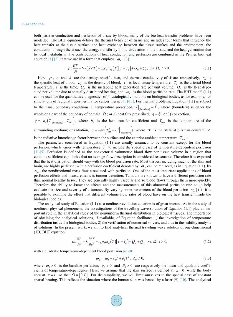
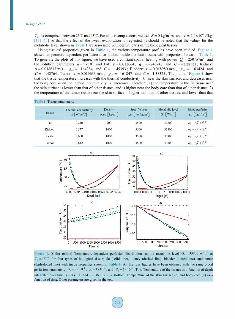
Using tissues’ properties given in Table 1, the various temperature profiles have been studied. Figure 1 shows temperature-dependent perfusion distributions inside the four tissues with properties shown in Table 1. To generate the plots of this figure, we have used a constant spatial heating with power 2250 W/mrQ = and the solution parameters 45 10a = × and Fat: 0.012664υ = , 1 246748g− = − and 2.28521C = − ; Kidney:

0.018613 m/sυ = , 1 164384g− = − and 1.45393C = − ; Bladder: 0.018980 m/sυ = , 1 163424g− = − and 1.42764C = − ; Tumor: 0.019633 m/sυ = , 1 161847g− = − and 1.38325C = − . The plots of Figure 1 show

that the tissue temperature increases with the thermal conductivity k near the skin surface, and decreases near the body core when the thermal conductivity k increases. Therefore, 1) the temperature of the fat tissue near the skin surface is lower than that of other tissues, and is higher near the body core than that of other tissues; 2) the temperature of the tumor tissue near the skin surface is higher than that of other tissues, and lower than that

Table 1. Tissue parameters.

Tissue Thermal conductivity

k [ ]W/m/ Density

3, kg/mbρ ρ Specific heat

3, Ws/kg/mbc c Metabolic level

3 W/mmQ Blood perfusion

3 kg/s/mmω

Fat 0.210 900 3500 33800 20 0 0T Tω γ δ+ +

Kidney 0.577 1000 3500 33800 20 0 0T Tω γ δ+ +

Bladder 0.600 1000 3500 33800 20 0 0T Tω γ δ+ +

Tumor 0.642 1000 3500 33800 20 0 0T Tω γ δ+ +

Figure 1. (Color online) Temperature-dependent perfusion distributions at the metabolic level 333800 W/mmQ = at 15 CfT = for four types of biological tissues fat (solid line), kidney (dashed line), bladder (dotted line), and tumor

(dash-dotted line) with tissue properties shown in Table 1. All the four figures have been obtained with the same blood perfusion parameters, 4

0 7 10ω −= × , 40 1 10γ −= × , and 6

0 7 10δ −= × . Top: Temperature of the tissues as a function of depth integrated over time 0 st = (a) and 3600 st = (b). Bottom: Temperature of the skin surface (c) and body core (d) as a function of time. Other parameters are given in the text.

E. Kengne et al.

727

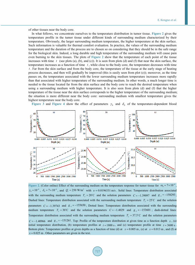
of other tissues near the body core. In what follows, we concentrate ourselves to the temperature distribution in tumor tissue. Figure 2 gives the

temperature profile in the tumor tissue under different kinds of surrounding medium characterized by their temperature. Obviously, the larger surrounding medium temperature, the higher temperature at the skin surface. Such information is valuable for thermal comfort evaluation. In practice, the values of the surrounding medium temperature and the duration of the process are to chosen so on considering that they should be in the safe range for the biological skin. Indeed, a long durable and high temperature of the surrounding medium will cause pain even burning to the skin tissues. The plots of Figure 2 show that the temperature of each point of the tissue increases with time t (see plots (a), (b), and (c)). It is seen from plots (d) and (f) that near the skin surface, the temperature increases as a function of time t , while close to the body core, the temperature decreases with time t . Far from the skin surface and from the body core, the temperature of the tissue at the early stage of heating process decreases, and then will gradually be improved (this is easily seen from plot (e)); moreover, as the time passes on, the temperature associated with the lower surrounding medium temperature increases more rapidly than that associated with higher temperature of the surrounding medium. In other words, a much longer time is needed to the tissue located far from the skin surface and the body core to reach the desired temperature when using a surrounding medium with higher temperature. It is also seen from plots (d) and (f) that the higher temperature of the tissue near the skin surface corresponds to the higher temperature of the surrounding medium; the situation is more different near the body core: surrounding medium with smallest temperature gives the highest temperature near the body core.

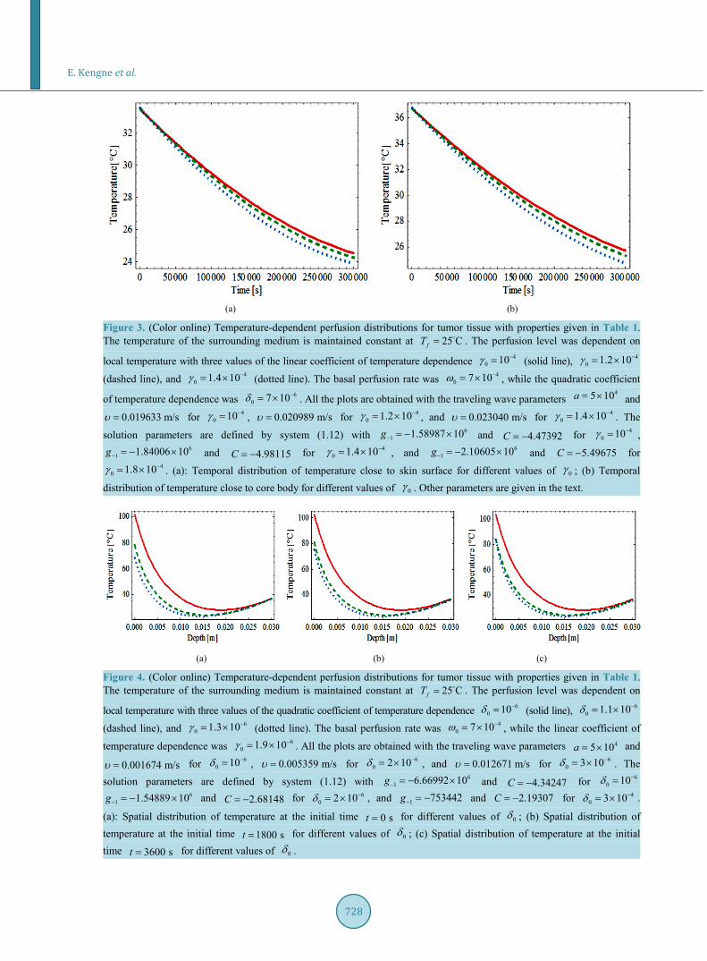
Figure 3 and Figure 4 show the effect of parameters 0γ and 0δ of the temperature-dependent blood

Figure 2. (Color online) Effect of the surrounding medium on the temperature response for tumor tissue for 40 7 10ω −= × ,

40 10γ −= , 6

0 7 10δ −= × , and 3250 W/mrQ = with 0.0196331 m/sυ = . Solid lines: Temperature distribution associated with the surrounding medium temperature 20 CfT = and the solution parameters 1.39097C = − and 1 = 158293g− − ;

Dashed lines: Temperature distribution associated with the surrounding medium temperature 25 CfT = and the solution

parameters 1.39743C = − and 1 155650g− = − ; Dotted lines: Temperature distribution associated with the surrounding medium temperature 30 CfT = and the solution parameters 1.4029C = − and 1 153601g− = − ; dash-dotted lines:

Temperature distribution associated with the surrounding medium temperature 37.5 CfT = and the solution parameters

1.40966C = − and 1 151261g− = − . Top: Profile of the temperature distribution at given time as a function depth x , (a) initial temperature distribution, (b) temperature profiles at 1800 st = , and (c) temperature profile at time 3600 st = . Bottom plots: Temperature profiles at given depths as a function of time (d) at 0.005 mx = , (e) at 0.013 mx = , and (f) at

0.025 mx = . Other parameters are given in the text.

E. Kengne et al.

728

(a) (b)

Figure 3. (Color online) Temperature-dependent perfusion distributions for tumor tissue with properties given in Table 1. The temperature of the surrounding medium is maintained constant at 25 CfT = . The perfusion level was dependent on

local temperature with three values of the linear coefficient of temperature dependence 40 10γ −= (solid line), 4

0 1.2 10γ −= ×

(dashed line), and 40 1.4 10γ −= × (dotted line). The basal perfusion rate was 4

0 7 10ω −= × , while the quadratic coefficient

of temperature dependence was 60 7 10δ −= × . All the plots are obtained with the traveling wave parameters

45 10a = × and

0.019633 m/sυ = for 40 10γ −= , 0.020989 m/sυ = for 4

0 1.2 10γ −= × , and 0.023040 m/sυ = for 40 1.4 10γ −= × . The

solution parameters are defined by system (1.12) with 61 1.58987 10g− = − × and 4.47392C = − for 4

0 10γ −= , 6

1 1.84006 10g− = − × and 4.98115C = − for 40 1.4 10γ −= × , and 6

1 2.10605 10g− = − × and 5.49675C = − for 4

0 1.8 10γ −= × . (a): Temporal distribution of temperature close to skin surface for different values of 0γ ; (b) Temporal distribution of temperature close to core body for different values of 0γ . Other parameters are given in the text.

(a) (b) (c)

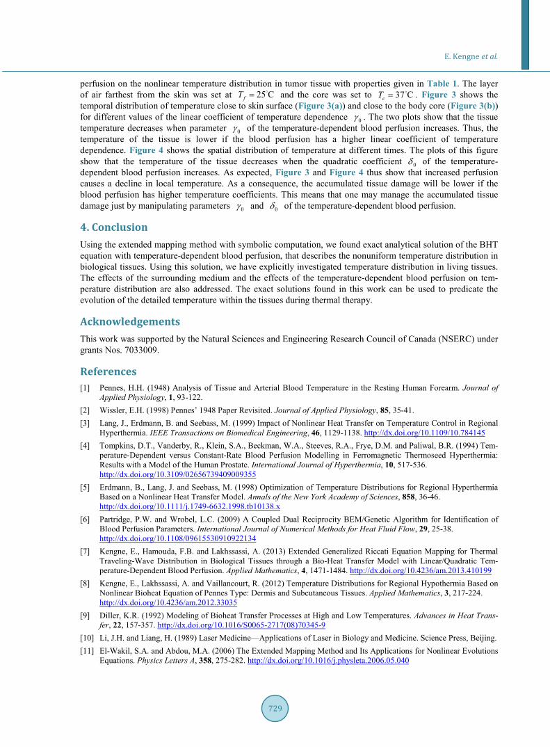
Figure 4. (Color online) Temperature-dependent perfusion distributions for tumor tissue with properties given in Table 1. The temperature of the surrounding medium is maintained constant at 25 CfT = . The perfusion level was dependent on

local temperature with three values of the quadratic coefficient of temperature dependence 60 10δ −= (solid line), 6

0 1.1 10δ −= ×

(dashed line), and 60 1.3 10γ −= × (dotted line). The basal perfusion rate was 4

0 7 10ω −= × , while the linear coefficient of

temperature dependence was 60 1.9 10γ −= × . All the plots are obtained with the traveling wave parameters 45 10a = × and

0.001674 m/sυ = for 60 10δ −= , 0.005359 m/sυ = for 6

0 2 10δ −= × , and 0.012671 m/sυ = for 60 3 10δ −= × . The

solution parameters are defined by system (1.12) with 61 6.66992 10g− = − × and 4.34247C = − for 6

0 10δ −= 6

1 1.54889 10g− = − × and 2.68148C = − for 60 2 10δ −= × , and 1 753442g− = − and 2.19307C = − for 4

0 3 10δ −= × .

(a): Spatial distribution of temperature at the initial time 0 st = for different values of 0δ ; (b) Spatial distribution of temperature at the initial time 1800 st = for different values of 0δ ; (c) Spatial distribution of temperature at the initial time 3600 st = for different values of 0δ .

E. Kengne et al.

729

perfusion on the nonlinear temperature distribution in tumor tissue with properties given in Table 1. The layer of air farthest from the skin was set at 25 CfT = and the core was set to 37 CcT = . Figure 3 shows the temporal distribution of temperature close to skin surface (Figure 3(a)) and close to the body core (Figure 3(b)) for different values of the linear coefficient of temperature dependence 0γ . The two plots show that the tissue temperature decreases when parameter 0γ of the temperature-dependent blood perfusion increases. Thus, the temperature of the tissue is lower if the blood perfusion has a higher linear coefficient of temperature dependence. Figure 4 shows the spatial distribution of temperature at different times. The plots of this figure show that the temperature of the tissue decreases when the quadratic coefficient 0δ of the temperature- dependent blood perfusion increases. As expected, Figure 3 and Figure 4 thus show that increased perfusion causes a decline in local temperature. As a consequence, the accumulated tissue damage will be lower if the blood perfusion has higher temperature coefficients. This means that one may manage the accumulated tissue damage just by manipulating parameters 0γ and 0δ of the temperature-dependent blood perfusion.

4. Conclusion Using the extended mapping method with symbolic computation, we found exact analytical solution of the BHT equation with temperature-dependent blood perfusion, that describes the nonuniform temperature distribution in biological tissues. Using this solution, we have explicitly investigated temperature distribution in living tissues. The effects of the surrounding medium and the effects of the temperature-dependent blood perfusion on tem- perature distribution are also addressed. The exact solutions found in this work can be used to predicate the evolution of the detailed temperature within the tissues during thermal therapy.

Acknowledgements This work was supported by the Natural Sciences and Engineering Research Council of Canada (NSERC) under grants Nos. 7033009.

References [1] Pennes, H.H. (1948) Analysis of Tissue and Arterial Blood Temperature in the Resting Human Forearm. Journal of

Applied Physiology, 1, 93-122. [2] Wissler, E.H. (1998) Pennes’ 1948 Paper Revisited. Journal of Applied Physiology, 85, 35-41. [3] Lang, J., Erdmann, B. and Seebass, M. (1999) Impact of Nonlinear Heat Transfer on Temperature Control in Regional

Hyperthermia. IEEE Transactions on Biomedical Engineering, 46, 1129-1138. http://dx.doi.org/10.1109/10.784145 [4] Tompkins, D.T., Vanderby, R., Klein, S.A., Beckman, W.A., Steeves, R.A., Frye, D.M. and Paliwal, B.R. (1994) Tem-

perature-Dependent versus Constant-Rate Blood Perfusion Modelling in Ferromagnetic Thermoseed Hyperthermia: Results with a Model of the Human Prostate. International Journal of Hyperthermia, 10, 517-536. http://dx.doi.org/10.3109/02656739409009355

[5] Erdmann, B., Lang, J. and Seebass, M. (1998) Optimization of Temperature Distributions for Regional Hyperthermia Based on a Nonlinear Heat Transfer Model. Annals of the New York Academy of Sciences, 858, 36-46. http://dx.doi.org/10.1111/j.1749-6632.1998.tb10138.x

[6] Partridge, P.W. and Wrobel, L.C. (2009) A Coupled Dual Reciprocity BEM/Genetic Algorithm for Identification of Blood Perfusion Parameters. International Journal of Numerical Methods for Heat Fluid Flow, 29, 25-38. http://dx.doi.org/10.1108/09615530910922134

[7] Kengne, E., Hamouda, F.B. and Lakhssassi, A. (2013) Extended Generalized Riccati Equation Mapping for Thermal Traveling-Wave Distribution in Biological Tissues through a Bio-Heat Transfer Model with Linear/Quadratic Tem-perature-Dependent Blood Perfusion. Applied Mathematics, 4, 1471-1484. http://dx.doi.org/10.4236/am.2013.410199

[8] Kengne, E., Lakhssassi, A. and Vaillancourt, R. (2012) Temperature Distributions for Regional Hypothermia Based on Nonlinear Bioheat Equation of Pennes Type: Dermis and Subcutaneous Tissues. Applied Mathematics, 3, 217-224. http://dx.doi.org/10.4236/am.2012.33035

[9] Diller, K.R. (1992) Modeling of Bioheat Transfer Processes at High and Low Temperatures. Advances in Heat Trans-fer, 22, 157-357. http://dx.doi.org/10.1016/S0065-2717(08)70345-9

[10] Li, J.H. and Liang, H. (1989) Laser Medicine—Applications of Laser in Biology and Medicine. Science Press, Beijing. [11] El-Wakil, S.A. and Abdou, M.A. (2006) The Extended Mapping Method and Its Applications for Nonlinear Evolutions

Equations. Physics Letters A, 358, 275-282. http://dx.doi.org/10.1016/j.physleta.2006.05.040

E. Kengne et al.

730

[12] Abdou, M.A. and Zhang, S. (2009) New Periodic Wave Solution via Extended Mapping Method. Communications in Nonlinear Science and Numerical Simulation, 14, 2-11. http://dx.doi.org/10.1016/j.cnsns.2007.06.010

[13] Weber L.W. and Pierce J.T. (2003) Development of Occupational Skin Disease. In DiNardi, S.R., Ed., The Occupa-tional Environment: Its Evaluation, Control and Management, 2nd Edition, AIHA Press, Virginia, 348-360.

[14] Kingma, B., Frijns, A. and van Marken Lichtenbelt, W. (2012) The Thermoneutral Zone: Implications for Metabolic Studies. Frontiers in Bioscience, 4, 1975-1985. http://dx.doi.org/10.2741/E518

[15] Ozisik, M.N. (1993) Heat Conduction. John Wiley & Sons, Inc., New York, 506-507. [16] Weinbaum, S., Jiji, L.M. and Lemons, D.E. (1984) Theory and Experiment for the Effect of Vascular Microstructure

on Surface Tissue Heat Transfer-Part I: Anatomical Foundation and Model Conceptualization. Journal of Biome-chanical Engineering, 106, 321-330. http://dx.doi.org/10.1115/1.3138501

[17] Liu, J. and Xu, L.X. (2000) Boundary Information Based Diagnostics on the Thermal States of Biological Bodies. In-ternational Journal of Heat and Mass Transfer, 43, 2827-2839. http://dx.doi.org/10.1016/S0017-9310(99)00367-1

Scientific Research Publishing (SCIRP) is one of the largest Open Access journal publishers. It is currently publishing more than 200 open access, online, peer-reviewed journals covering a wide range of academic disciplines. SCIRP serves the worldwide academic communities and contributes to the progress and application of science with its publication. Other selected journals from SCIRP are listed as below. Submit your manuscript to us via either submit@scirp.org or Online Submission Portal.