Embed Size (px)
Citation preview
May 16, 2005 13:13 WSPC/129-JBS 00147
Journal of Biological Systems, Vol. 13, No. 2 (2005) 151–171c© World Scientific Publishing Company
A MATHEMATICAL MODEL FOR SPATIALLY EXPANDINGINFECTED AREA OF EPIDEMICS TRANSMITTEDTHROUGH HETEROGENEOUSLY DISTRIBUTED
SUSCEPTIBLE UNITS
SHINKO KOSHIBA
Department of Information and Computer Sciences, Faculty of ScienceNara Women’s University, Nara 630-8506, Japan
HIROMI SENO∗
Department of Mathematical and Life Sciences, Graduate School of ScienceHiroshima University, Higashi-hiroshima 739-8526, Japan
Received 1 June 2004Revised 25 October 2004
Little is known about the effect of environmental heterogeneity on the spatial expansionof epidemics. In this work, to focus on the question of how the extent of epidemic dam-age depends on the spatial distribution of susceptible units, we develop a mathematicalmodel with a simple stochastic process, and analyze it. We assume that the unit of infec-tion is immobile, as town, plant, etc. and classify the units into three classes: susceptible,infective and recovered. We consider the range expanded by infected units, the infectedrange R, assuming a certain generalized relation between R and the total number ofinfected units k, making use of an index, a sort of fractal dimension, to characterizethe spatial distribution of infected units. From the results of our modeling analysis, weshow that the expected velocity of spatial expansion of infected range is significantlyaffected by the fractal nature of spatial distribution of immobile susceptible units, andis temporally variable. When the infection finally terminates at a moment, the infectedrange at the moment is closely related to the nature of spatial distribution of immobilesusceptible units, which is explicitly demonstrated in our analysis.
Keywords: Epidemics; Stochastic Process; SIR Model; Fractal Dimension; Velocity.
1. Introduction
A variety of infectious diseases show different seriousness in terms of the infectedarea expansion, depending not only on the infectivity but also on the characteristicsof infected place, city, or country: the environment-dependent way of disease trans-mission and the sanitary/health condition determine the nature of infected area
∗Corresponding author.
151

May 16, 2005 13:13 WSPC/129-JBS 00147
152 Koshiba & Seno
expansion.1–3 However, little is known about the effect of environmental hetero-geneity on the spatial expansion of epidemics. In reality, a variety of species expandtheir spatial distribution depending on their ecological characteristics, settling theirhabitats composed of patchy environments, for instance, of trees, of wetland, or ofmountains.3–13 Especially, in case of plants or crops under attack from pests anddiseases, the spatial distribution of susceptible hosts is considered as important forthe spread of infection.3,14–18
So we can regard such a spatially patchy/fragmentated habitat as the collectionof immobile units for infection of an epidemic disease transmitted within a consid-ered population which inhabits in the habitat. Jules et al.17 studied an invasion ofnon-native root pathogen, Phytophthora lateralis, over a heterogeneous landscapeof its host, Port Orford cedar, Chamaecyparis lawsoniana, the population of whichis restricted to riparian zones along creeks. In human case, we may consider thetown or the village as such unit. Such patchiness of population distribution can bediscussed from the viewpoint of fractal, too.12,13,19–25
As for spatially transmitted disease dynamics, a variety of researches with math-ematical model have been studied,3,26 making use of, for instance, reaction-diffusionsystem,27–32 integro-differential or integro-difference equations,33–38 percolationtheory or network theory,18,39–46 cellular automaton or lattice dynamics.14,47–50
Especially, mathematical models with percolation theory or network theory havebeen attracting researchers who are interested in the invasion threshold which isthe critical condition to determine weather the infection stops in a finite period orkeeps its spatial expansion.
In this paper, with a mathematical model, we consider the effect of spatial dis-tribution of susceptible units (cities, communities, plants, nests, etc.) on the natureof spatial expansion of disease infected region. Especially we focus on the velocityof its spatial expansion, which has been theoretically discussed in various contextsmostly with mathematical models used reaction-diffusion system (for instance, seeRefs. 27, 28, 30–32 and their references). In contrast, we therefore try to discussthe characteristics of velocity with a mathematical model making use of a stochas-tic process. The velocity of spatial expansion of disease infected region must beaffected by the nature of spatial distribution of susceptible units. In our model-ing, to incorporate the effect of heterogeneous spatial distribution of susceptibleunits on the spatial expansion of disease infected region, we characterize the spatialdistribution with an index, fractal dimension,22 and introduce it into our model.So our model describes the epidemic population dynamics with a stochastic pro-cess, and the spatial expansion of disease infected region with a fractal nature ofspatial distribution of susceptible units. This type of combination of populationdynamics and spatial expansion may be regarded as an approximation for the realinter-relationship between them. We show that our modeling would be useful toget theoretical insights or develop the more advanced or practical model about thespatial expansion of disease infected area.

May 16, 2005 13:13 WSPC/129-JBS 00147
Mathematical Model for Expanding Infected Area 153
2. Modeling
2.1. Assumptions
In our modeling, we assume that the unit of infection is immobile, as town, plant,etc. We classify the units into three classes, depending on the state in terms ofthe disease infection: susceptible, infective and recovered. Susceptible unit is not yetinfected, and infective one has been transmitted the disease and is still carryingit so as to transmit the disease to another unit. Recovered unit was infected inthe past but is recovered so as not to transmit the disease to any other unit. Itcould correspond to the unit with immunity after its recovery from the disease. Sothis modeling can be regarded as a kind of SIR epidemic dynamics.27,28,30,32 Sincethe recovered unit has no relation to the disease transmission dynamics, we couldregard it as a completed destroyed or abandoned unit due to the disease infection,though the expression “recovered” is not appropriate in this context.
We do not consider the population/epidemic dynamics within each unit, butclassify the unit as mentioned above in terms of its epidemic state of the diseaseinfection. In this sense, our model would be regarded as belonging to the metapop-ulation model.51
To construct our mathematical model, we assume the following:
• Infection rate depends only on the total number of infective units.• Only susceptible unit could be infected.• Recovered unit is never infected again.• Infection and recovery of a unit are independent of those of any other units.
The first assumption corresponds, for instance, to the case that the epidemic vectorhas a high mobility to transmit the disease, or the case that the disease transmissionis through the matrix environment (e.g. wind, water or soil) surrounding susceptibleunits.16,18,39
In this paper, we consider the number of infective units, h, and that of infectedunits which is the sum of infective and recovered, k. Infected unit is an infective orrecovered one, that is, a unit which experienced the disease transmission.
2.2. Model construction
2.2.1. Probability for infection
With the assumptions given in the previous section, we consider events occurringin sufficiently short time interval (t, t + ∆t] when h infective units exist at time t.
Probability that a susceptible unit has been transmitted the disease by an infec-tive unit is assumed to be given by β∆t + o(∆t) independently of the distancebetween them, where β is a positive constant, the infection rate. Since we assumethat the infection of a susceptible unit by an infective unit is independent of that by

May 16, 2005 13:13 WSPC/129-JBS 00147
154 Koshiba & Seno
any other infective one, the probability that a susceptible unit has been transmittedthe disease by h infective units becomes
βh∆t + o(∆t). (2.1)
Probability that more than one susceptible units have been transmitted the diseaseduring sufficiently small period ∆t is assumed to be o(∆t). Hence, the probabilitythat none of the susceptible units has been transmitted the disease during suffi-ciently small period ∆t is given by
1 − [βh∆t + o(∆t)] − o(∆t) = 1 − βh∆t − o(∆t). (2.2)
2.2.2. Probability for recovery
Probability that an infective unit recovers during sufficiently small period ∆t isassumed to be given by
γ∆t + o(∆t), (2.3)
where γ is a positive constant, the recovery rate.When there are h infective units, the probability that only one infective unit
recovers is given by the probability for the case when the recovery of an infectiveunit occurs with probability given by (2.3) and at the same time the other h − 1infective units do not recover with probability given by [1−{γ∆t+o(∆t)}]h−1. Thisis because the probability that an infective unit does not recover is 1−{γ∆t+o(∆t)},and the epidemic state of each unit is assumed to be independent of that of anyother unit.
Therefore, taking account of which infective unit of h recovers, the requiredprobability is obtained as follows:
h · {γ∆t + o(∆t)} · [1 − {γ∆t + o(∆t)}]h−1
= h · {γ∆t + o(∆t)} · {1 − (h − 1)γ∆t + o(∆t)}= γh∆t + o(∆t). (2.4)
Probability that more than one infective units recover is assumed to be o(∆t).Thus, from (2.4), the probability that none of the infective units recovers duringsufficiently small period ∆t is given by
1 − γh∆t − o(∆t). (2.5)
From the assumption of independence between infection and recovery, the prob-ability that both infection and recovery occur during the time period ∆t is givenby o(∆t), because the probability for each of them has the order ∆t at the highest.

May 16, 2005 13:13 WSPC/129-JBS 00147
Mathematical Model for Expanding Infected Area 155
2.2.3. Probability distribution for epidemic state
We denote by P (k, h, t) the probability of epidemic state such that there are k
infected units and h infective units at time t in the considered system. To determinethe probability P (k, h, t), we consider the transition of state in sufficiently smalltime interval (t, t + ∆t], and derive the system of differential equations that governthe temporal variation of probability P (k, h, t).
With transition probabilities for possible transitions of epidemic state in suf-ficiently small time interval (t, t + ∆t] as derived in Appendix A, we can get thefollowing differential equations for P (k, h, t) (Appendix B):
dP (k, h, t)dt
= −(β + γ)hP (k, h, t) + γ(h + 1)P (k, h + 1, t)
+ β(h − 1)P (k − 1, h − 1, t), (2.6)
for k ≥ 2, h ≥ 1, k ≥ h + 1, and
dP (k, 0, t)dt
= γP (k, 1, t), (2.7)
dP (k, k, t)dt
= −k(β + γ)P (k, k, t) + (k − 1)βP (k − 1, k − 1, t) (2.8)
for k ≥ 1.
2.2.4. Initial condition
We assume that the epidemic begins at a unit, so that the initial condition isgiven by
P (k, h, 0) ={
1 if k = h = 1,
0 otherwise.(2.9)
2.2.5. Expansion of infected range
Next, we consider the range expanded by infected units, say, the infected range.We characterize the infected range by the minimal diameter R which includes allinfected units.
In the case when the infected range expands in every direction with the sameprobability, the shape of infected region can be approximated by the disc, andtherefore, the range R approximately has the following relation with the number ofinfected units k: k ∝ R2. However, the expansion of infected range is constrainedby the spatial distribution of potential carriers for the considered disease, whichcould be in general heterogeneous. So the shape of infected region is possibly inho-mogeneous in direction, and could be characterized by its fractal nature (for theconcept of “fractal” (see Refs. 22 and 52). To deal with such a case, we assume thefollowing generalized relation between the infected range and the total number ofinfected units:
k ∝ Rd (1 ≤ d ≤ 2), (2.10)

May 16, 2005 13:13 WSPC/129-JBS 00147
156 Koshiba & Seno
(a) (b) (c)
Fig. 1. Illustrative explanation of the relation of the fractal dimension d to the spatial pattern ofunit distribution. Schematic procedure of disease transmission is also shown: White disc indicatessusceptible unit, black infective, and grey recovered. (a) d ≈ 1; (b) 1 < d < 2; and (c) d ≈ 2.
where the power d characterizes the spatial pattern of infected region occupied byinfected units (Fig. 1). Power d is called cluster dimension or mass dimension, whichis a sort of fractal dimension.22,52 When d ≈ 2, the spatial distribution of infectedunits has approximately a disc shape of its envelope. When d ≈ 1, the distributioncan be approximately regarded as one-dimensional, that is, the infected units canbe regarded to be arrayed along a curve.
For instance, Port Orford cedar, Chamaecyparis lawsoniana, is the host for theroot pathogen, Phytophthora lateralis, and has a heterogeneous population distri-bution, because it is restricted to riparian zones along creeks.17 The populationdistribution of Port Orford cedar, Chamaecyparis lawsoniana, would be character-ized with the fractal dimension d such that 1 < d < 2 (see Fig. 1).
This idea of introduction of fractal nature into the mathematical model for thespatial distribution of units is the same as that in Seno.53 This modeling may beregarded as a sort of mean-field approximation for the percolation process on a frac-tal lattice or the growing network. However, we focus on the temporal variation ofthe spatial range spanned by infected susceptible units, differently from most of pre-vious works with the percolation theory or the growing network theory.18,39,40,42–46
Some percolation models for the epidemic dynamics considered the fractalnature of susceptible unit distribution, too.46 In such previous models, the mainproblem was the invasion threshold which is the critical condition to determine

May 16, 2005 13:13 WSPC/129-JBS 00147
Mathematical Model for Expanding Infected Area 157
Fig. 2. Illustrative explanation of range R(2).
whether the infection stops in a finite period or keeps its spatial expansion. In con-trast, we are going to focus on the velocity of spatial expansion of infected range.
For convenience to apply the relation (2.10) for our modeling, we now definethe proportional constant C:
k = CRd (1 ≤ d ≤ 2). (2.11)
Then, we define the mean distance R(2) from one unit to the nearest neighbor(Fig. 2). In our modeling, R(2) is assumed to correspond to the expected infectedrange expanded by two infected units, that is, k = 2. Therefore, from (2.11), weassume that
2 = CRd(2). (2.12)
Hence, from (2.11), for the expected number of infected units 〈k〉t at time t, weassume the following relation with the expected infected range rt at time t:
〈k〉t = 2rdt (1 ≤ d ≤ 2), (2.13)
where rt is the expected infected range at time t, measured in the mean distanceR(2): rt ≡ Rt/R(2).
Further, we define the expected velocity Vt of the expansion of infected range attime t as follows:
Vt =drt
dt.
From (2.13), we can obtain the following relation between the expected velocity Vt
and the expected number 〈k〉t of infected units at time t:
Vt =1d
(12
)1/d
〈k〉1/d−1t · d〈k〉t
dt. (2.14)

May 16, 2005 13:13 WSPC/129-JBS 00147
158 Koshiba & Seno
3. Analysis
3.1. Expected number of infective units
We denote by 〈h〉t the expected number of infective units at time t. It is defined by
〈h〉t =∞∑
k=1
k∑h=1
hP (k, h, t). (3.1)
Hence, from (2.6) and (2.8), we can obtain the following:
d
dt〈h〉t = (β − γ)〈h〉t,
that gives
〈h〉t = e(β−γ)t, (3.2)
where we used the initial condition (2.9) for (3.1): 〈h〉0 = 1.
3.2. Expected number of infected units
We denote by 〈k〉t the expected number of infected units at time t, defined by
〈k〉t =∞∑
k=1
k
{k∑
h=0
P (k, h, t)
}. (3.3)
From (2.6), (2.7) and (2.8), we can obtain the following:
d
dt〈k〉t = β〈h〉t.
With (3.2), we can solve this differential equation and get the following:
〈k〉t =β
β − γ{e(β−γ)t − 1} + 1, (3.4)
where we used the initial condition (2.9) for (3.3): 〈k〉0 = 1.We can get the saturated value for 〈k〉t. From (3.4), for β ≥ γ when the infection
rate is not less than the recovery rate, the saturate value becomes positively infinite,that is, any saturation to a finite value does not occur. On the other hand, for β < γ
when the recovery rate is greater than the infection rate, the saturated value is finite,and is given by
〈k〉t→∞ =γ
γ − β. (3.5)

May 16, 2005 13:13 WSPC/129-JBS 00147
Mathematical Model for Expanding Infected Area 159
3.3. Expected infected range
Since, from (2.13),
rt =( 〈k〉t
2
)1/d
, (3.6)
we can consider how the expected infected range rt depends on the fractal dimensiond for the spatial distribution of susceptible units, making use of (3.4). For 0 <
β/γ < 1/2, when the recovery rate is sufficiently greater than the infection rate,the expected infected range rt gets larger as d is larger (Fig. 3a). This means thatthe infected range is expected to become wider as the susceptible units are moreuniformly distributed. In contrast, for β/γ ≥ 1/2, the expected infected range getssmaller as d is larger (Figs. 3b–3d). In this case, the infected range is expected tobe narrower as the susceptible units are more uniformly distributed. Therefore, inour model, only if the infection rate is smaller than half of the recovery rate, themore uniform distribution of susceptible units causes the wider expected infectedrange (see Fig. 4).
Now, we consider the saturated value of expected infected range as t → ∞.From (3.4) and (3.6), for β > γ when the infection rate is greater than the recovery
(a) (b)
(c) (d)
Fig. 3. Temporal development of the expected infected range. (a) 0 < β/γ < 1/2, calculated forβ = 0.3 and γ = 0.8; (b) 1/2 ≤ β/γ ≤ 1, calculated for β = 0.3 and γ = 0.5; (c) 1 < β/γ < d,calculated for β = 0.55 and γ = 0.5; and (d) β/γ ≥ d, calculated for β = 0.55 and γ = 0.5.

May 16, 2005 13:13 WSPC/129-JBS 00147
160 Koshiba & Seno
(a) (b)
Fig. 4. d-dependence of the saturated value of expected infected range. (a) 0 < β/γ < 1/2,calculated for β = 0.3 and γ = 0.8 and (b) β/γ ≥ 1/2, calculated for β = 0.3 and γ = 0.5.
(a) (b)
Fig. 5. Temporal variation of the expected expansion velocity of infected range. (a) 0 < β/γ ≤ 1,calculated for β = 0.3 and γ = 0.5; (b) 1 < β/γ < d, calculated for β = 0.5 and γ = 0.4; and (c)β/γ ≥ d, calculated for β = 0.5 and γ = 0.4.
rate, the value becomes positively infinite as t → ∞ (Figs. 3c and 3d). On theother hand, for β < γ when the recovery rate is greater than the infection rate, itis saturated to the following value as t → ∞ (Figs. 3a and 3b):
rt→∞ =( 〈k〉t→∞
2
)1/d
=(
12· γ
γ − β
)1/d
. (3.7)
3.4. Expected expansion velocity of infected range
When β/γ ≤ 1, that is, when the recovery rate is not less than the infection rate,the expected velocity Vt given by (2.14) monotonically decreases in time (Fig. 5a).
When 1 < β/γ < d, the expected velocity Vt decreases in the earlier periodand then turns to increase monotonically (Fig. 5b). We denote by tc the time whenthe expected velocity turns from decreasing to increasing. From (2.14), we can

May 16, 2005 13:13 WSPC/129-JBS 00147
Mathematical Model for Expanding Infected Area 161
(c)
Fig. 5. (Continued).
explicitly get
tc =1
β − γln
γ
βd. (3.8)
When β/γ ≥ d, the expected velocity Vt monotonically increases in time(Fig. 5c).
At last, we can see how the expected velocity Vt depends on the fractal dimensiond for the spatial distribution of susceptible units. The expected velocity gets smalleras d is larger (Figs. 5a–5c) for any value of β/γ. Therefore, in our model, the moreuniform distribution of susceptible units causes the slower expansion of infectedrange.
3.5. Probability of termination of infection
We denote by Ph=0 the probability of termination of infection. Once an infectiveunit disappears in space because of recovery, the infection can no longer continueand restart. If the infection terminates at time t, for sufficiently small ∆t, theepidemic state should be with only one infective unit at time t − ∆t, and theinfective unit should recover during ∆t without causing any new infection. Whenthe number of infected units is k at time t, from (2.2) and (2.3), the probability forthis event is given by
P (k, 1, t)[1 − β∆t − o(∆t)] · [γ∆t + o(∆t)] = γP (k, 1, t)∆t + o(∆t). (3.9)
Therefore, the probability for the termination of infection between t − ∆t and t isgiven by the sum of (3.9) over any possible k.
Making use of the probability generating function (p.g.f.) defined by
f(x, y, t) =∞∑
k=1
k∑h=0
P (k, h, t)xkyh, (3.10)

May 16, 2005 13:13 WSPC/129-JBS 00147
162 Koshiba & Seno
we can derive the probability for the termination of infection (as for the p.g.f., seeAppendix C):
Ph=0 =∫ ∞
0
γ
∞∑k=1
P (k, 1, t)dt
=∫ ∞
0
γ · ∂f
∂y
∣∣∣∣x=1,y=0
dt
=∫ ∞
0
γ · e−(β−γ)t{(β − γ)/β}2
1 − e−(β−γ)tγ/βdt
= min{
γ
β, 1}
. (3.11)
The probability Ph=0 is 1 for β ≤ γ when the recovery rate is greater than theinfection rate (Fig. 6). This case is when the infection certainly terminates in afinite time. When the infection rate is greater than the recovery rate, the probabilityPh=0 is proportional to the recovery rate and inversely proportional to the infectionrate (Fig. 6).
3.6. Expected time for the termination of infection
We denote by 〈t〉h=0 the expected time for the termination of infection. From thearguments in the previous section, we can explicitly obtain
〈t〉h=0 =∫ ∞
0
tγ∞∑
k=1
P (k, 1, t)dt
=
+∞ if β ≥ γ;
1β
lnγ
γ − βif β < γ.
(3.12)
For β < γ when the recovery rate is greater than the infection rate, we can expectthat the infection terminates at a finite time. In this case, the expected time gets
(a) (b)
Fig. 6. Parameter dependence of the probability for the termination of infection, Ph=0.(a) β-dependence and (b) γ-dependence.
May 16, 2005 13:13 WSPC/129-JBS 00147
Mathematical Model for Expanding Infected Area 163
(a) (b)
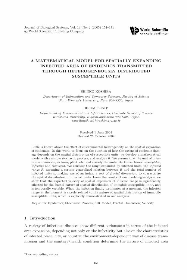
Fig. 7. Parameter dependence of the expected time for the termination of infection 〈t〉h=0.(a) β-dependence and (b) γ-dependence.
longer as the infection rate is greater, and shorter as the recovery rate is greater(Fig. 7).
3.7. Expected number of infected units at the termination
of infection
We denote by 〈k〉h=0 the expected number of infected units at the termination ofinfection. Integral
∫∞0 γP (k, 1, t)dt gives the probability that the number of infected
units is k at the moment when the infection terminates. Therefore, making use ofthe p.g.f. (3.10) and (4.4) in Appendix C, we can get
〈k〉h=0 =∞∑
k=1
k
∫ ∞
0
γP (k, 1, t)dt
= γ
∫ ∞
0
∞∑k=1
kP (k, 1, t)dt
= γ
∫ ∞
0
∂
∂y
(∂f
∂x
)∣∣∣∣x=1,y=0
dt
= γ
∫ ∞
0
∂
∂x
(∂f
∂y
∣∣∣∣y=0
)∣∣∣∣∣x=1
dt
=γ
γ − β. (3.13)
From (3.5) and (3.13), we can see that the expected number of infected units atthe termination of infection, 〈k〉h=0 is identical to the saturated value of 〈k〉t, thatis, 〈k〉t→∞:
〈k〉h=0 = 〈k〉t→∞.
Therefore, 〈k〉h=0 has the characteristics same as for 〈k〉t→∞. The expected rangeat the termination of infection is also identical to the saturated range of rt, thatis, rt→∞.

May 16, 2005 13:13 WSPC/129-JBS 00147
164 Koshiba & Seno
4. Discussion
In this work, to focus on the question of how the extent of epidemic damage dependson the spatial distribution of susceptible units, we constructed a mathematicalmodel with a simple stochastic process, and analyzed it.
We assumed that the unit of infection is immobile, as town, plant, etc. and clas-sify the units into three classes: susceptible, infective and recovered. This modelingcan be regarded as a kind of SIR epidemic dynamics.27,28,30,32 We do not considerthe population/epidemic dynamics within each unit, but classify the unit as men-tioned above in terms of its epidemic state in terms of the disease infection. In thissense, our model would be regarded as belonging to the metapopulation model.51
Our modeling is not always unrealistic or over-idealized. In reality, a variety ofspecies expand their spatial distributions, settling their habitats composed of patchyenvironments, for instance, of trees, of wetland, or of mountains.3,8,10–16,18 So wecan regard each patch of such spatially fragmentated habitats as the immobile unitof infection for an epidemic disease transmitted within the population. In humancase, we may consider the town or the village as such unit.
In our model, we considered the probability for the state such that k infectedand h infective units exist at time t. Infected unit is an infective or recoveredone, that is, a unit which experienced the disease transmission. Infective unit hasbeen transmitted the disease and is still carrying it so as to transmit the diseaseto another unit. Recovered unit was transmitted the disease in the past and hasrecovered so as not to transmit the disease to any other unit. So it could correspondto the unit with immunity after its recovery from the disease. Since the recoveredunit has no relation to the disease transmission dynamics, we could regard it as acompletely destroyed or abandoned unit due to the disease infection, though theexpression “recovered” is not appropriate in this context.
We derived the system of differential equations to describe the temporal varia-tion of the probability distribution in terms of the numbers of infected and infec-tive units. Furthermore, we considered the mathematical modeling for the rangeexpanded by infected units in space ,the infected range R, which can be character-ized by the expected minimal diameter R which includes all infected units. In ourmodeling, we assumed a generalized relation between R and the total number ofinfected units k, making use of an index called cluster dimension or mass dimension,that is a sort of fractal dimension, which characterizes the spatial distribution ofsusceptible units. With the generalized relation, we can develop the mathematicalmodel for the temporal variation of expected infected range and of expected expan-sion velocity of infected range. From our analysis of the model, we showed that theexpected velocity is significantly affected by the nature of spatial distribution ofimmobile susceptible units, and is temporally variable, differently from those typ-ical results derived for the mathematical model with the reaction-diffusion systemin continuous space.
Consequently we found three types of temporal variation of expected veloc-ity of infected range expansion, depending on the fractal dimension of spatial

May 16, 2005 13:13 WSPC/129-JBS 00147
Mathematical Model for Expanding Infected Area 165
distribution of susceptible units: monotonically decreasing, monotonically decreas-ing, and increasing after initially decreasing. The last case implies that we haveto pay attention to the expansion of infected area even if the velocity of its spa-tial expansion is observed to decrease in the early period of disease transmissionprocess.
In our modeling, a susceptible unit has been transmitted the disease andbecomes infective with probability proportional to the total number of infectiveunits, that is, the total number of patchy habitats with active disease carriers,as in Seno and Matsumoto54 who analyzed a mathematical model for populationdynamics to expand its spatial distribution with patch creation by the existingwhole population. This assumption corresponds, for instance, to the case that theepidemic vector has a high mobility to transmit the disease, or the case that thedisease transmission is through the matrix environment (e.g. wind, water or soil)surrounding susceptible units.16,18,39
It may be more realistic that a susceptible unit would have transmitted the dis-ease via some spatially neighbor infective units. This assumption requires anothermodeling and would make the model more difficult to be mathematically analyzed.Some cellular automaton models or lattice models have been considered such diseasetransmission in space. Computer-aided numerical analysis has always been usefulin the analysis of such models, whereas numerical calculations could not derive thegeneral result about the nature of spatial disease transmission. To consider only aspecific disease transmission in space, it might be satisfactory with some specificparameter values. However, as indicated in some well-known mathematical worksabout epidemics, for example, the Kermack-McKendrick model,55 this does notmean less evaluation of theoretically/mathematically general results from mathe-matical models in mathematical biology. Only a few mathematical methods couldreach some general features of such models, for instance, the mean field approxi-mation and the pair approximation, etc.15,48,50,56
In this paper, we consider our mathematical model in the context of spatialexpansion of infected range of epidemic disease transmitted via immobile suscep-tible units. However, our modeling is easily applied in the case of the spatiallyexpanding population distribution through patchy/fragmentated habitats in space.In this context, the parameter β can be regarded as the settlement rate from anestablished habitat to another newly immigrated one, and γ as the rate to abandonor destroy a settled habitat. If the considered population is of a harmful insect tobe exterminated, γ may be regarded as the exterminated rate for a unit aggregatedby the insect.
For the spatial expansion of population distribution, some well-known mathe-matical models are of reaction-diffusion system in spatially continuous space.30–32,57
However, in general, it is not easy or is more tactical to introduce the natureof spatial heterogeneity of habitat distribution into such models with reaction-diffusion system. In contrast, in the case of spatially discrete models, frequentlyconstructed by cellular automaton or lattice space,18,39,50,58 introduction of spatial

May 16, 2005 13:13 WSPC/129-JBS 00147
166 Koshiba & Seno
heterogeneity is relatively easy, whereas mathematical analysis is rarely easy andbecomes harder as the number of factors governing the dynamics increases, sothat a number of numerical calculations are required. Stochastic model like ours isanother way for the theoretical study that could give some new insights, as indi-cated in some papers of landscape ecology.59–61 Our model could be regarded asone that is between a non-spatial population dynamics model and a numerical one,and may be termed a semi-spatial model as called by Filipe et al.48 Since there hasbeen few models to consider the velocity of spatial expansion of infected region withsuch spatially discrete susceptible units, we hope that our modeling considerationwould be a pioneer approach to the problem.
References
1. Gilligan CA, An epidemiological framework for disease management, Adv Bot Res38:1–64, 2002.
2. Keeling MJ, Woolhouse MEJ, Shaw DJ, Matthews L, Chase-Topping M, HaydonDT, Cornell SJ, Kappey J, Wilesmith J, Grenfell BT, Dynamics of the 2001 UKfoot and mouth epidemic: stochastic dispersal in a heterogeneous landscape, Science294:813–817, 2001.
3. van den Bosch F, Mets JAJ, Zadoks JC, Pandemics of focal plant disease: a model,INTERIM REPORT IR-97-083, 1997.
4. Anderson RM, May RM, The invasion, persistence and spread of infectious diseasewithin animal and plant communities, Philos Trans R Ser B 314:533–570, 1986.
5. Andow DA, Kareiva PM, Levin SA, Okubo A, Spread of invading organisms, LandsEcol 4:177–188, 1990.
6. Dwyer G, Elkinton JS, Buonaccorsi JP, Host heterogeniety in susceptibility and dis-ease dynamics: tests of a mathematical model, Am Nat 150:685–707, 1997.
7. Jeger MJ, Spatial Component of Plant Disease Epidemics, Prentice-Hall, EnglewoodCliffs, 1989.
8. Johnson AR, Wiens JA, Milne BT, Crist TO, Animal movements and populationdynamics in heterogeneous landscapes, Lands Ecol 7:63–75, 1992.
9. Levin SA, The problem of pattern and scale in ecology, Ecology 73:1943–1967, 1992.10. Neuhauser C, Mathematical challenges in spatial ecology, Not AMS 48:1304–1314,
2001.11. O’Neill RV, Milne BT, Turner MG, Gardner RH, Resource utilization scales and
landscape pattern, Lands Ecol 2:63–69, 1988.12. Russell RW, Hunt Jr GL, Coyle KO, Cooney RT, Foraging in a fractal environment:
spatial patterns in a marine predator-prey system, Lands Ecol 7:195–209, 1992.13. With KA, The landscape ecology of invasive spread, Conserv Biol 16:1192–1203, 2002.14. Brown DH, Bolker BM, The effects of disease dispersal and host clustering on the
epidemic threshold in plants, Bull Math Biol 66:341–371, 2004.15. Caraco T, Duryea MC, Glavanakov S, Host spatial heterogeneity and the spread of
vector-borne infection, Theor Pop Biol 59:185–206, 2001.16. Drenth A, Fungal epidemics — does spatial structure matter?, New Phytol 163:4–7,
2004.17. Jules ES, Kauffman MJ, Ritts WD, Carroll AL, Spread of an invasive pathogen
over a variable landscape: a non-native root rot on Port Orford cedar, Ecology 83:3167–3181, 2002.
May 16, 2005 13:13 WSPC/129-JBS 00147
Mathematical Model for Expanding Infected Area 167
18. Otten W, Bailey DJ, Gilligan CA, Empirical evidence of spatial thresholdsto control invasion of fungal parasites and saprotrophs, New Phytol 163:125–132, 2004.
19. Gautestad AO, Mysterud I, Fractal analysis of population ranges: methodologicalproblems and challenges, Oikos 69:154–157, 1994.
20. Haskell JP, Ritchle ME, Olff H, Fractal geometry predicts varying body size scalingrelationships for mammal and bird home ranges, Nature 418:527–530, 2002.
21. Keymer JE, Marquet PA, Velasco-Hernandez JX, Levin SA, Extinction thresholdsand metapopulation persistence in dynamic landscapes, Am Nat 156:478–494, 2000.
22. Mandelbrot BB, Fractal Geometry of Nature, W.H. Freeman and Company, New York,1982.
23. Morse DR, Lawton JH, Dodson MM, Williamson MH, Fractal dimension ofvegetation and the distibution of arthropod body lengths, Nature 314:731–733,1985.
24. With KA, Using fractal analysis to assess how species perceive landscape structure,Lands Ecol 9:25–36, 1994.
25. With KA, King AW, Extinction thresholds for species in fractal landscapes, ConservBiol 13:314–326, 1999.
26. Metz JAJ, Mollison D, van den Bosch F, The dynamics of invasion waves, INTERIMREPORT IR-99-039, 1999.
27. Brauer F, Castillo-Chavez C, Mathematical models in population biology and epi-demiology, in Texts in Applied Mathematics, Vol. 40, Springer, New York, 2001.
28. Diekmann O, Heesterbeek JAP, Mathematical epidemiology of infectious diseases:model building, analysis and interpretation, in Wiley Series in Mathematical andComputational Biology, John Wiley & Sons, Chichester, 2000.
29. Fagan WF, Lewis MA, Neubert MG, van den Driessche P, Invasion theory and bio-logical control, Ecol Lett 5:148–157, 2002.
30. Murray JD, Introduction to mathematical biology, in Interdisciplinary Applied Math-ematics, Vol. 17, Springer, New York, 2002.
31. Murray JD, Mathematical biology: spatial models and biomedical applications, 3rdedition, Interdisciplinary Applied Mathematics, Vol. 18, Springer, New York, 2002.
32. Shigesada N, Kawasaki K, Biological Invasions: Theory and Practice, Oxford Univer-sity Press, New York, 1997.
33. Atkinson C, Reuter GEH, Deterministic epidemic waves, Math Proc Camb Philos Soc80:315–330, 1976.
34. Brown K, Carr J, Deterministic epidemic waves of critical velocity, Math Proc CambPhilos Soc 81:431–433, 1977.
35. Kot M, Schaffer WM, Discrete-time growth-dispersal models, Math Biosci 80:109–136, 1986.
36. Medlock J, Kot M, Spreading disease: integro-differential equations old and new, MathBiosci 184:201–222, 2003.
37. Mollison D, Spatial contact models for ecological and epidemic spread, J R Stat SocB 39:283–326, 1977.
38. Neubert MG, Kot M, Lewis MA, Invasion speeds in fluctuating environments, ProcR Soc Lond B 267:1603–1610, 2000.
39. Bailey DJ, Otten W, Gilligan CA, Saprotrophic invasion by the soil-borne fun-gal plant pathogen Rhizoctonia solani and percolation thresholds, New Phytol 146:535–544, 2000.
40. Grassberger P, On the critical-behaviour of the general epidemic process and dynam-ical percolation, Math Biosci 63:157–172, 1983.

May 16, 2005 13:13 WSPC/129-JBS 00147
168 Koshiba & Seno
41. Keeling MJ, The effects of local spatial structure on epidemiological invasions, ProcR Soc Lond B 266:859–867, 1999.
42. Meyers LA, Newman MEJ, Martin M, Schrag S, Applying network theory to epi-demics: control measures for Mycoplasma pneumoniae outbreak, Emerg Infect Dis9:204–210, 2003.
43. Newman MEJ, Spread of epidemic disease on networks, Phys Rev E 66:016128,2002.
44. Sander LM, Warren CP, Sokolov IM, Simon C, Koopman J, Percolation onheterogeneous networks as a model for epidemics, Math Biosci 180:293–305,2002.
45. Stauffer D, Aharony A, Introduction to Percolation Theory, Taylor & Francis, London,1991.
46. Tan Z-J, Zou X-W, Jin Z-Z, Percolation with long-range correlations for epidemicspreading, Phys Rev E 62:8409–8412, 2000.
47. Filipe JAN, Gibson GJ, Studying and approximating spatio-temporal models for epi-demic spread and control, Philos Trans R Soc Lond B 353:2153–2162, 1998.
48. Filipe JAN, Gibson GJ, Gilligan CA, Inferring the dynamics of a spatial epidemicfrom time-series data, Bull Math Biol 66:373–391, 2004.
49. Levin SA, Durrett R, From individuals to epidemics, Philos Trans R Soc Lond B351:1615–1621, 1997.
50. Sato K, Matsuda H, Sasaki A, Pathogen invasion and host extinction in lattice struc-tures populations, J Math Biol 32:251–268, 1994.
51. Hanski I, Metapopulation Ecology, Oxford University Press, Oxford, 1999.52. Hastings HM, Sugihara G, Fractals: A User’s Guide for the Natural Sciences, Oxford
University Press, New York, 1993.53. Seno H, Stochastic model for colony dispersal, Anthropol Sci 101:65–78, 1993.54. Seno H, Matsumoto H, Stationary rank-size relation for community of logistically
growing groups, J Biol Syst 4:83–108, 1996.55. Kermack WO, McKendrick AG, A contribution to the mathematical theory of epi-
demics, Philos R Soc Lond A 115:700–721, 1927.56. Filipe JAN, Gibson GJ, Comparing approximations to spatio-temporal models for
epidemics with local spread, Bull Math Biol 63:603–624, 2001.57. Okubo A, Levin SA, Diffusion and ecological problems: modern perspectives, 2nd
edition, in Interdisciplinary Applied Mathematics, Vol. 14, Springer, New York, 2001.58. Rhodes CJ, Jensen HJ, Anderson RM, On the critical behaviour of simple epidemics,
Proc R Soc Lond B 264:1639–1646, 1997.59. Dunning JB, Stewart DJ, Danielson BJ, Noon BR, Root TL, Lamberson RH, Stevens
EE, Spatially explicit population models: current forms and future uses, Ecol Appl5:3–11, 1995.
60. Fortin M-J, Boots B, Csillag F, Remmel TK, On the role of spatial stochastic modelsin understanding landscape indices in ecology, Oikos 102:203–212, 2003.
61. Wiegand T, Moloney KA, Naves J, Knauer F, Finding the missing link betweenlandscape structure and population dynamics: a spatially explicit perspective, AmNat 154:605–627, 1999.
62. Bailey NTJ, The Mathematical Theory of Epidemics, Charles Griffin & Co. Ltd.,London, 1957.

May 16, 2005 13:13 WSPC/129-JBS 00147
Mathematical Model for Expanding Infected Area 169
Appendix A
To determine the probability P (k, h, t), we consider respectively the following tran-sitions of state in sufficiently small time interval (t, t + ∆t].
(k, h, t) → (k, h, t + ∆t): In this case, since there is no change in the numberof infected units and that of infective ones, neither infection nor recovery occursduring time period ∆t. Therefore, from (2.2) and (2.5), the transition probabilityis given by
[1 − βh∆t − o(∆t)] · [1 − γh∆t − o(∆t)] = 1 − (β + γ)h∆t + o(∆t). (4.1)
(k − 1, h, t) → (k, h, t + ∆t): Since only the number of infected units increasesby one, one infection and one recovery should occur during time period ∆t. Toincrease the number of infected units by one, the number of infective units mustincrease by one. Hence, in order that the number of infective units at t + ∆t issimultaneously h, the number of infective units must decrease by one during ∆t.From the assumption given in the previous section, both infection and recoveryoccur during ∆t with probability o(∆t), so that the considered transition probabilityis o(∆t), too.
(k, h + 1, t) → (k, h, t + ∆t): In this case, only one recovery occurs during timeperiod ∆t with no change in the number of infected units, when any new infectiondoes not occur. Therefore, from (2.2) and (2.4), the transition probability is given by
[1 − β(h + 1)∆t − o(∆t)] · [γ(h + 1)∆t + o(∆t)] = γ(h + 1)∆t + o(∆t). (4.2)
(k − 1, h − 1, t) → (k, h, t + ∆t): In this case, one infection occurs without anyrecovery during time period ∆t. Therefore, from (2.1) and (2.5), the transitionprobability is given by
[β(h − 1)∆t + o(∆t)] · [1 − γh∆t − o(∆t)] = (h − 1)β∆t + o(∆t). (4.3)
(k − l, h − l, t) → (k, h, t + ∆t) (l ≥ 2): In this case, infection occurs l timeswithout any recovery during time period ∆t. Since more than one infection occursduring ∆t, the transition probability is o(∆t).
(k, h + m, t) → (k, h, t + ∆t) (m ≥ 2): In this case, recovery occurs m timeswithout any infection during ∆t. Since more than one recovery occurs during ∆t,the transition probability is o(∆t).
(k − l, h + n, t) → (k, h, t + ∆t) (n ≥ 0; 1 ≤ l ≤ k − 1): In this case, infec-tion and recovery occur l and n + l times, respectively during ∆t. Since more thanone infection and recovery occurs during ∆t, the transition probability is o(∆t).

May 16, 2005 13:13 WSPC/129-JBS 00147
170 Koshiba & Seno
Appendix B
With transition probabilities (4.1), (4.2) and (4.3) for possible transitions of statein sufficiently small time interval (t, t + ∆t], we can derive the following equationfrom the definition of P (k, h, t) for k ≥ 1, h ≥ 0, k ≥ h + 1:
P (k, h, t + ∆t) = P (k, h, t) · [1 − (β + γ)h∆t + o(∆t)]
+ P (k, h + 1, t) · [γ(h + 1)∆t + o(∆t)]
+ P (k − 1, h − 1, t) · [(h − 1)β∆t + o(∆t)]
+∞∑l=2
P (k − l, h− l, t) · o(∆t)
+∞∑
m=2
P (k, h + m, t) · o(∆t)
+k−1∑l=1
∞∑n=0
P (k − l, h + n, t) · o(∆t).
Therefore, we can obtain the equation for {P (k, h, t + ∆t) − P (k, h, t)}/∆t], andthen as ∆t → 0, we can get the differential equation (2.6).
Appendix C
From (3.10), applying (2.6) to (2.8) with a cumbersome and careful calculation, wecan derive the following partial differential equation for the probability generatingfunction (p.g.f.) f(x, y, t) defined by (3.10):
∂f(x, y, t)∂t
= {−(β + γ)y + γ + βxy2}∂f(x, y, t)∂y
. (4.1)
From (2.9), the initial condition is given by
f(x, y, 0) =∞∑
k=1
k∑h=0
P (k, h, 0)xkyh
= P (1, 1, 0)xy
= xy. (4.2)
In addition, the following condition can be derived:
f(1, 1, t) =∞∑
k=1
k∑h=0
P (k, h, t) = 1, (4.3)
because the sum of probability for any possible k and h corresponds to the occur-rence of any event.

May 16, 2005 13:13 WSPC/129-JBS 00147
Mathematical Model for Expanding Infected Area 171
With condition (4.2) and (4.3), we can directly solve (4.1) as follows:62
f(x, y, t) = x ·[v+(x) − v(x){v+(x) − y}
Φ(x)
], (4.4)
where
Φ(x) = {v+(x) − y} + {y − v−(x)}e−βxv(x)t;
v(x) = v+(x) − v−(x),
and v+(x) and v−(x) are functions of x, given by two distinct roots of the followingequation in terms of ξ:
βxξ2 − (β + γ)ξ + γ = 0.