Embed Size (px)
Citation preview

Experimental investigation of the seabed roughness effect on the hydrodynamicalbehavior of a submarine cable under current and wave conditions.
A. Marty(1),*, G. Damblans(2), J-V. Facq(1), B. Gaurier(1), G. Germain(1), N.Germain(2), J. Harris(4), A. Maison(2), C. Peyrard(3), and N. Relun(3)
(1)IFREMER, Marine Structure Laboratory, 150 Quai Gambetta, Boulogne/Mer, France(2)France Energies Marines, Brest, France
(3)EDF R&D, 6 Quai Watier, 78400 Chatou, France(4)LHSV, Ecole des Ponts, CEREMA, EDF R&D, Chatou, France
*Corresponding author: [email protected]
Resume
Le comportement des cables sous-marins est etudie experimentalement dans le cadre du projet France En-ergies Marines STHYF. Dans le but d’evaluer la stabilite des cables lorsqu’ils sont places sur des fonds avecde grandes rugosites et soumis a de fortes conditions de vagues et de courants, les efforts hydrodynamiquesqui se produisent sur un cylindre fixe place a proximite d’une plaque sur laquelle est positionne ou nondes elements de rugosites ont ete mesures. Des sollicitations specifiques (courant, oscillations forcees etoscillations + courant) sont imposees afin de quantifier les efforts hydrodynamiques exerces sur le cylindreplace a differents distances de la plaque (avec ou sans rugosite). Les effets de la rugosite sur les effortsappliques au cylindre et sur l’ecoulement sont etudies et mettent en evidence des differences importantesentre la configuration fond rugueux et fond lisse. Les efforts hydrodynamiques qui s’appliquent sur lecylindre sont notamment plus faibles lorsque celui est proche d’un fond rugueux que d’un fond lisse. Deplus les coefficients de traınee statique et oscillante sont largement plus faibles dans le cas rugueux quedans le cas lisse. Les coefficients d’inertie presentent moins de differences significatives entre les differentsecartements etudies.
Summary
Submarine cable behaviour is experimentally studied in the frame of the France Energies Marines projectSTHYF. In order to evaluate on-bottom stability of cables placed on rocky seabed with high roughnessand submitted to combined wave and strong current, hydrodynamic loads are measured on a fixed slendercylinder closely fixed to a horizontal plate, with or without large roughness. A specified set of load cases(forced oscillations, current, forced oscillation + current) is considered to assess the hydrodynamic loadsacting on the cylinder placed near a wall for varying gap-to-diameter ratios. The roughness effects oncylinder loads and on the flow are studied in detail. The result show a significant difference between roughand smooth bottom configurations. Indeed, the loads measurements and hydrodynamic coefficients aresignificantly lower with the presence of a rough plate near the cylinder. Especially for drag and oscillatorydrag coefficients, however the inertia coefficient presents less differences between the different studiedgaps.
1

1. Introduction
Flow around a cylinder in unbounded condition has been studied extensively because of its interesting flowfeatures and practical applications [1]. On the contrary, the flow around a cylinder in proximity to a wall hasbeen less studied even if this kind of study has direct application to many engineering problems such as powercables of marine renewable energy systems.In [2], large-eddy simulations are used to investigate the modifications of the wake dynamics and turbulencecharacteristics behind a circular cylinder placed near a wall for varying gap-to-diameter ratios. In this study,the shear layer transition, stretching, breakdown and turbulence generation have been studied for a Reynoldsnumber of 1440, in the presence of a smooth wall under steady conditions. Submarine pipelines and power ca-bles at intermediate and shallow waters are subjected to wave and current induced forces. In these conditions,the incident flow separates from the cylinder producing a vortex shedding regime in the near field. The flowseparation induces drag and lift hydrodynamic forces which become relevant in comparison with the inertiaones.An essential step for pipeline and power cable design is the accurate evaluation of these hydrodynamic forces.An experimental work on three types of soil has been carried out by Zhou and al. [3] in order to studythe seabed responses around a marine pipeline under wave and current conditions, but with no forces mea-surements on the cylinder. Aristodemo [4] proposes a numerical model to determine horizontal and verticalcomponents of the hydrodynamic forces on a slender submarine pipeline lying on the sea bed and exposed tonon-linear waves plus a current. The comparison between experimental and numerical hydrodynamic forcesshows the accuracy of the new model in evaluating the time variation of peaks and phase shifts of the hori-zontal and vertical wave and current induced forces. Unfortunately, the seabed roughness effect has not beentaken into account in these works (or only for small roughness). It is thus necessary to conduct specific studiesin order to study the large seabed roughness effects on the structural loads.In this study, submarine cable behaviour is experimentaly studied in order to study on-bottom stability of ca-bles placed on rocky seabed with high roughness and submitted to combined wave and strong current (up to5m/s), as for example in the Alderney Race, France. For that purpose, hydrodynamic loads are measured ona fixed slender cylinder closely fixed to a horizontal plate, with or without large roughness. A specified set ofload cases (forced oscillations, current, forced oscillation + current) is considered to assess the hydrodynamicloads acting on the cylinder placed near a wall for varying gap-to-diameter ratios.The present work is organized as follows: in the second section the experimental set-up is presented; after-wards, the roughness effects on cylinder loads are studied in section 3.
2. Experimental set-up
2.1 Flume tank and assembly
Tests were carried out in the wave and current circulating flume tank of IFREMER located in Boulogne-sur-Mer(France). The incoming flow is assumed to be steady and constant inside the test section of 18 m long × 4 mwide × 2 m deep. By means of a grid combined with a honeycomb (that acts as a flow straightener) placedat the inlet of the working section, a low turbulent intensity of I = 1.5 % is achieved. In this work, the threeinstantaneous velocity components are denoted (U,V,W ) along the (x,y,z) directions respectively (see figure1). Using the Reynolds decomposition, each instantaneous velocity component is separated into a mean valueand a fluctuation part: U(X , t) =U(X)+u′(X , t), where an overbar indicates the time average.A specific assembly is needed to reproduce submarine cable environment, mainly the boundary layer perceivedby the cable due to a rough seabed and the wave influence. Combined waves and current effects act on a bottomcylinder as an oscillatory velocity at the seabed of um with a period T , and a background current velocity U .Here, we neglect the vertical motion of the fluid due to the wave. We only take into account in this study thehorizontal component of the orbital wave velocity on the seabed. So, um = um (x, t), imposed by the motionof the assembly by a six degrees of freedom motion generator, able to impose horizontal motion of amplitude
2

0.4 m at a frequency between 0.1 and 0.4 Hz, with a precision better than one mm.
Figure 1. Drawing view of the experimental set-up with the horizontal plate fixed at 0.5 m below the free surface.
The rough seabed is represented by the use of a flat plate (2 m x 1.5 m), fixed horizontally to the motiongenerator by the use of a specific frame at a depth of 0.5 m from the free surface, as shown in figure 2. Seabedroughness (kbed
s ) is here modeled by the use of square blocks fixed on the plate, regularly spaced as shown onfigure 1.
Figure 2. CAD view of the experimental set-up with the frame fixed under the hexapod for the rough bottomconfiguration.
The cylinder is fixed between two rows of roughness at the center of the plate, perpendicular to the upstreamflow. In this study, the model scale is fixed at 1:2.6. Thus, the diameter of the rigid cylinder is fixed atD = 0.05 m and the size of the square blocs at 0.08 m × 0.08 m × 0.3 m (see figure 3).
Figure 3. Cylinder fixed under a flat (left) and rough plate (right).
In order to study the boundary layer effects on the cable behaviour, different gaps, denoted e, between thecylinder and the plate have been considered. Four gaps from 2 mm to 2.5 D have been considered with asmooth plate and four gaps from 1 D to 2.5 D with the rough plate, as shown on figure 4. Only one kind ofcylinder has been used: a smooth cylinder (weight∼ 5 kg). In the following, non dimensional lengths are usedfor all parameters indexed by ∗: x∗ = x/D, for instance, with D the diameter of the cylinder of length L. Themain characteristics of the experimental set-up are summarized in Table 1.
3

Figure 4. Drawing view of the different configurations, with and without seabed roughness.
Scale D e/D kcyls kbed
s U∞
- [m] - [m] [m] [m/s]1:1 0.13 [0 ; 2.5] [0 ; 0.006] [0.01 ; 0.2] [0 ; 2.5]
1:2.6 0.05 [0 ; 2.5] 0 - 0.002 0 - 0.08 [0 ; 0.75]
Table 1. In situ and experimental conditions.
2.2 Load and flow measurements
Two 2-component force gauges, of range: Fx,z = 100 N, are used to measure the hydrodynamic forces onthe cylinder. They are connected at the vertical arm extremity, at each side of the plate, as shown on figure5. The 1.235 m long cylinder is fixed between them by the mean of needle roller bearings. The cylinder isthen free in rotation and translation so as not to exert pre-stress during assembly. No cylinder motions havebeen encountered during measurements, with comparable measurements between both load-cells (reflecting aperfect forces distribution along the cylinder). The drag and lift forces (respectively FD and FL) are then:
FD (t) = Fx1 (t) + Fx2 (t)FL (t) = Fz1 (t) − Fz2 (t)
Figure 5. Drawing view of the force measurement system (left) and view of the cylinder fixed between two load cells(surrounded in red) under the smooth plate (right).
The flow around the cylinder location is characterized from PIV (Particle Image Velocimetry) measurements,see figure 6. Beforehand, the tank is seeded with 10 µm diameter silver coated glass particles. A Nd-YAG
Laser GEMINI-LIKE is used: power is 200 mJ per probe and wavelength is 532 mm. The laser emission issynchronized with a Camera FLOWSENS EO-2M 1600pix× 1200pix that makes double images with a timestep of 1600 µs.In these conditions, a particle is detected on 3 to 5 pixels, cross-correlation peak intensity is between 0.3 and0.8 and peak detectability is 8 in average [5]. PIV acquisitions are made for 150 s, with a 15 Hz acquisitionfrequency hence 2250 double images are acquired for all cases. The data are post processed with DYNAMIC
STUDIO. Particles displacement is calculated using a Cross-Correlation. Outliers are then replaced with the
4
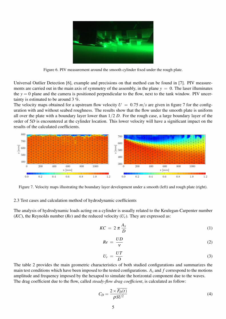
Figure 6. PIV measurement around the smooth cylinder fixed under the rough plate.
Universal Outlier Detection [6], example and precisions on that method can be found in [7]. PIV measure-ments are carried out in the main axis of symmetry of the assembly, in the plane y = 0. The laser illuminatesthe y = 0 plane and the camera is positioned perpendicular to the flow, next to the tank window. PIV uncer-tainty is estimated to be around 3 %.The velocity maps obtained for a upstream flow velocity U = 0.75 m/s are given in figure 7 for the config-uration with and without seabed roughness. The results show that the flow under the smooth plate is uniformall over the plate with a boundary layer lower than 1/2 D. For the rough case, a large boundary layer of theorder of 5D is encountered at the cylinder location. This lower velocity will have a significant impact on theresults of the calculated coefficients.
400
500
600
700
800
0 200 400 600 800 1000
z[m
m]
x [mm]
0.0 0.2 0.4 0.6 0.8 1.0 1.2
300
400
500
600
700
0 200 400 600 800 1000
z[m
m]
x [mm]
0.0 0.2 0.4 0.6 0.8 1.0 1.2
Figure 7. Velocity maps illustrating the boundary layer development under a smooth (left) and rough plate (right).
2.3 Test cases and calculation method of hydrodynamic coefficients
The analysis of hydrodynamic loads acting on a cylinder is usually related to the Keulegan-Carpenter number(KC), the Reynolds number (Re) and the reduced velocity (Ur). They are expressed as:
KC = 2 πAx
D(1)
Re =UDν
(2)
Ur =UTD
(3)
The table 2 provides the main geometric characteristics of both studied configurations and summarizes themain test conditions which have been imposed to the tested configurations. Ax and f correspond to the motionsamplitude and frequency imposed by the hexapod to simulate the horizontal component due to the waves.The drag coefficient due to the flow, called steady-flow drag coefficient, is calculated as follow:
CD =2×FD(t)
ρSU2 (4)
5

Configuration D e/D kcyls /D kbed
s /D U Ax f Re/104 KC[m] - - - [m/s] [mm] [Hz] - -
flat plate 0.05 0 - 2.5 0 0 0.25 - 0.75 100 - 400 0.1 - 0.4 0.125 - 0.375 12 - 50rough plate 0.05 0 - 2.5 0 1.6 0.25 - 0.75 100 - 400 0.1 - 0.4 0.125 - 0.375 12 - 50
Table 2. Main geometric characteristics and test conditions imposed to the tested configurations
with ρ the density of water (ρ = 998 kg/m3), S = D×L the cylinder section in front of the flow and U thecurrent velocity. The notation FD(t) indicates the temporal mean of the drag FD(t).In the case of oscillating motions, the hexapod moves along the Ox axis, colinear to the current. The hexapodmovements are oscillating with an amplitude Ax and a pulse ω = 2π f such as: x(t) = Ax cos(ωt +ϕx). Itis assumed that the response of this excitation is a sinusoidal function as well (with Fm the amplitude, theharmonics higher than 1 are neglected). Thus, the drag force may be expressed as follows:
FD(t) = Fm cos(ωt +ϕF) (5)
Hence, with ϕ = ϕF −ϕx it comes :
FD(t) =−Fm cos(ϕ)
Ax ω2 x(t)+Fm sin(ϕ)
Ax ωx(t) (6)
This equation 6 can be compared with the Morison equation [8] :
FD(t) =−ρCmLπD2
4x(t)+
12
ρCdDL x(t) |x(t)| (7)
with Cm the inertia coefficient and Cd the drag coefficient. Moreover, sinωt |sinωt| can be approximated withsinωt, and more precisely with :
sinωt |sinωt| ' 83π
sinωt (8)
And finally, by comparison : Cm =
Fm cos(ϕ)
ρLπD2
4 Ax ω2
Cd =Fm sin(ϕ)
43π
ρDLA2x ω2
(9)
These coefficients are the same as the standard API [9] and are called Inertia and Drag Coefficients.For current and imposed wave-type motion cases it is assumed that the drag force can be divided into twoparts, the mean drag part FD(t) and the oscillating part Fm cos(ωt +ϕF), such as :
FD(t) = FD(t)+Fm cos(ωt +ϕF) (10)
Thus, the three coefficients CD, Cm ans Cd can be calculated similarly as previous (equations 4 and 9).
3. Roughness effect on cylinder loads
3.1 Current only test
The figure 8 presents the evolution of the mean drag loads as a function of the flow speed for the flat plateconfiguration (left) and the rough plate configuration (right) for each gap between the cylinder and the plate(see figure 4). In the studied flow range, there is a significant drag force difference between the two configu-rations. For the flat plate, the drag force reaches approximately 20 N whereas for the rough plate the max of
6

the drag force reaches 7 N. Moreover, in the flat case there is a difference of about 25% between the smallergap and the other cases, this difference does not apply in the rough plate configuration where the evolutionis more homogeneous. The choice has been made to represent the standard deviation of each measurementrepresented by the error bars on the graph. The results show that the standard deviation is relatively low inboth cases, about 5% of the higher measurement in the flat plate configuration and about 12% for the roughone.
0
5
10
15
20
25
0.2 0.3 0.4 0.5 0.6 0.7 0.8
FD[N
]
U [m/s]
e=0.04De=0.5De=1De=2.5D
0
5
10
15
20
25
0.2 0.3 0.4 0.5 0.6 0.7 0.8
FD[N
]U [m/s]
e=1De=1.5De=2De=2.5D
Figure 8. Drag force vs flow speed for the flat plate (left) and the rough one (right).Error bars represents the standard deviation of the measurement.
These figures highlight that there are no big fluctuations of the drag forces in current only cases even if thefluctuation is slightly higher with the presence of rough bottom. This phenomenom can be explain by the factthat in the studied gap range (1−2.5D), the cylinder stays inside the boundary layer developed by the presenceof roughness and equal to approximately 5D, as we can see in the figure 7 (right), while for the smooth plate,the cylinder is in the boundary layer only for the first gap (e = 0.004 D).
0
0.5
1
1.5
2
104 105
CD
Re
e=0.04De=0.5De=1De=2.5D
0
0.5
1
1.5
2
104 105
CD
Re
e=1De=1.5De=2De=2.5D
Figure 9. Drag coefficient CD vs Reynolds number for the flat plate (left) and the rough plate (right).
The variation of the mean drag coefficient CD for both configurations is presented in the figure 9. The cal-culated range values is significantly higher for the flat plate case which is between 0.82 for the smaller gap(0.04D) and 1.36 for the bigger one (2.5D). The values of CD in the flat plate configuration and relatively farfrom the plate are close to those provided in the research literature for a circular cylinder in a steady flow(see [10]), whereas for the rough configuration the values range is between 0.12 for the smaller gap, and 0.39for the bigger one. Overall, the closer the plate and the cylinder are, the lower the drag coefficient and thedrag forces are. Here the coefficients are calculated from the upstream flow speed (U∞) and not with the oneperceived by the cylinder. In the boundary layer induced by the roughness, the local flow velocity perceivedby the cylinder is 5 to 10 times lower than the upstream flow speed. The associated drag coefficient can thenreach high values.
7

Figure 10 presents the dependency of the Strouhal number, St =f×DU , on the Reynolds number. In this formula,
f corresponds to the first excitation frequency of the lift force measured on the cylinder. A constant value ofSt = 0.2 is observed for the smooth configuration. This value is very close to the Strouhal number commonlyused which is generally equal to 0.21, see [11]. For the rough configuration, the Strouhal number drops to avalue of about 0.1.
0
0.05
0.1
0.15
0.2
0.25
0.3
104 105
St
Re
e=0.04De=0.5De=1De=2.5D
0
0.05
0.1
0.15
0.2
0.25
0.3
104 105
St
Re
e=1De=1.5De=2De=2.5D
Figure 10. Experimental Strouhal number vs Reynolds number for the flat plate (left) and the rough plate (right).
0
0.05
0.1
0.15
0.2
0.25
104 105
C′ l
Re
e=0.04De=0.5De=1De=2.5D
0
0.05
0.1
0.15
0.2
0.25
104 105
C′ l
Re
e=1De=1.5De=2De=2.5D
Figure 11. Lift coefficient standard deviation Cl vs Reynolds number for the flat plate (left) and the rough plate (right).
The variation of the r.m.s values of the lift fluctuations with the Reynolds number is shown in figure 11. Inthe flat plate configuration, a maximum value of approximately 0.2 is obtained for range values of studiedReynolds numbers and for medium gaps (0.5D and 1D). This value drops to almost zero in the closer gapcase. In the rough plate configuration, the variation of C′l is more homogeneous and shows a slight decreasefor each gap, between 0.05 and 0.1.These results show that the rough bottom has an influence on the drag coefficient, the r.m.s. values of the liftfluctuations and the Strouhal number. The vortices are shed into the wake with different frequencies.
3.2 Oscillating motions
The figure 12 presents the evolution of the mean drag forces in function of Kc for the flat plate case (left) andthe rough plate case (right) for the oscillating motion test cases. The standard deviation of each measurementis represented by the error bars on the graph. There are several points at each Kc studied because several testshave been carried out at the same motion amplitude Ax but with different frequencies. As expected the meandrag loads is equal to zero for both configurations as there is no current, but the standard deviation calculatedfor each test shows that it increases for the smooth plate case, by a factor of two approximately.
8

−50
−40
−30
−20
−10
0
10
20
30
40
50
10 15 20 25 30 35 40 45 50 55
FD[N
]
KC
e=0.04De=0.5De=1De=2.5D
−50
−40
−30
−20
−10
0
10
20
30
40
50
10 15 20 25 30 35 40 45 50 55
FD[N
]
KC
e=1De=1.5De=2De=2.5D
Figure 12. Drag force vs Reynolds number for the flat plate on the left and the rough plate on the right.Error bars represents the standard deviation of the measurement.
The evolution of the oscillating drag coefficient Cd for the flat plate case (left) and the rough plate case (right)in function of Kc is represented in the figure 13. The calculated range values of the flat plate case is between 1.2for the smaller gap (0.04D) and 2.6 for the bigger gap (2.5D). For the rough configuration the range values isbetween 0.25 for the 1D gap and 2 for the 2.5D gap. This comparison does not highlight significant differencesfor the maximum range values. However, for the rough configuration the minimum value is decreased by afactor of 4 compared to the flat plate configuration.
0
0.5
1
1.5
2
2.5
3
10 15 20 25 30 35 40 45 50 55
Cd
KC
e=0.04De=0.5De=1De=2.5D
0
0.5
1
1.5
2
2.5
3
10 15 20 25 30 35 40 45 50 55
Cd
KC
e=1De=1.5De=2De=2.5D
Figure 13. Oscillating drag coefficient CD vs KC for the flat plate on the left and the rough plate on the right.
The figure 14 shows similarly the inertia coefficient Cm as a function of KC. The calculated range valuesis between 0.8 and 6 for the flat configuration and between 1 and 3 for the rough one. The presence of arough plate in vicinity of the cylinder reduces significantly the inertia coefficient. In both cases, calculatedcoefficients show an opposite behaviour concerning the gap between the cylinder and the plate. We clearly seethat the higher values are for the smaller gap case in the flat plate configuration. Whereas in the rough plateconfiguration, the closer case (1D) has the lower values. Overall, the behaviour of the cylinder shows thatoscillating drag coefficients and inertia coefficients are significantly lower with the presence of a rough plate.
3.3 Current and oscillating motions
The present section outlines results concerning current and oscillating motions tested cases. The figure 15shows the evolution of the mean drag force in function of the reduced speed Ur for the flat plate case (left)and the rough plate case (right) for each gap between the cylinder and the plate. As previously, the standarddeviation of each measurement is represented by an error bar on the graph.Contrary to the oscillating motion only case, the mean drag forces are not equal to zero anymore, especially
9

0
1
2
3
4
5
6
7
8
10 15 20 25 30 35 40 45 50 55
Cm
KC
e=0.04De=0.5De=1De=2.5D
0
1
2
3
4
5
6
7
8
10 15 20 25 30 35 40 45 50 55
Cm
KC
e=1De=1.5De=2De=2.5D
Figure 14. Added mass coefficient Cm vs KC for the flat plate on the left and the rough plate on the right.
in the flat plate case where the mean drag force can reach 39 N for a Kc equal to 38. However, in the roughplate configuration, these mean drag forces reach a maximum of 10 N for a Kc equal to 38 but is less than5 N in most cases with a small standard deviation as if it was in an oscillating motion only configuration. Thepresence of the rough plate near the cylinder reduces both mean drag forces and standard deviation by 30%.
−60
−40
−20
0
20
40
60
80
100
0 20 40 60 80 100 120 140 160
FD[N
]
Ur
e=0.04De=0.5De=1De=2.5D
−60
−40
−20
0
20
40
60
80
100
0 20 40 60 80 100 120 140 160
FD[N
]
Ur
e=1De=1.5De=2De=2.5D
Figure 15. Drag force vs Reduced velocity Ur for the flat plate on the left and the rough plate on the right.Error bars represents the standard deviation of the measurement.
The same coefficients previously shown, the mean drag coefficient CD, the oscillating drag coefficient Cd andthe added mass coefficient Cm are respectively represented in the figures 16, 17 and 18 in function of thereduced speed Ur .
0
1
2
3
4
5
0 20 40 60 80 100 120 140 160
CD
Ur
e=0.04De=0.5De=1De=2.5D
0
1
2
3
4
5
0 20 40 60 80 100 120 140 160
CD
Ur
e=1De=1.5De=2De=2.5D
Figure 16. Mean drag coefficient CD vs Reduced velocity Ur for the flat plate on the left and the rough plate on the right.
10

0
5
10
15
20
25
30
35
40
0 20 40 60 80 100 120 140 160
Cd
Ur
e=0.04De=0.5De=1De=2.5D
0
5
10
15
20
25
30
35
40
0 20 40 60 80 100 120 140 160
Cd
Ur
e=1De=1.5De=2De=2.5D
Figure 17. Oscillating drag coefficient Cd vs Reduced velocity Ur for the flat plate on the left and the rough plate (right).
The mean drag coefficient CD and the oscillating drag coefficient Cd are significantly higher in the case ofthe flat plate configuration compare to the rough one. Almost four times higher for CD and more than twotimes higher for Cd . As seen previously, the roughness drastically decreases the parameter values linked todrag phenomena by decreasing locally the mean flow speed. A change of behaviour is clear at Ur ≈ 60. ForUr ≤ 60, the cylinder behaviour is mainly driven by the static drag for both kinds of bottom while for Ur ≥ 60the cylinder behaviour is driven by the oscillating drag and the inertia coefficient (whatever the gap is).
0
2
4
6
8
10
0 20 40 60 80 100 120 140 160
Cm
Ur
e=0.04De=0.5De=1De=2.5D
0
2
4
6
8
10
0 20 40 60 80 100 120 140 160
Cm
Ur
e=1De=1.5De=2De=2.5D
Figure 18. Added mass coefficient Cm vs Reduced velocity Ur for the flat plate on the left and the rough plate (right).
Moreover the roughness seems to have less impact on inertia phenomena. Indeed, the range values of theadded mass is nearly the same in presence of a smooth or a rough bottom as we can see in figure 18.Furthermore, as for the oscillating case, the behavior of the Cm coefficient is opposite if we are in rough orflat configuration. We clearly see that the higher values are for the case 0.04D in the flat plate configuration,whereas in the rough plate configuration, the closer case (1D) has the lower values.
4. Conclusion and Perspectives
This study shows the impact of a plate with large roughness on the drag and inertia coefficients measured ona cylinder located near to it. The results are compared to the results obtained with a smooth bottom configura-tion. From these results, the evolution of the drag and inertia coefficients measured on the cylinder submittedto several test conditions (forced oscillations, current, forced oscillation + current) can be studied. Resultsshow that a rough bottom has an important impact on the hydrodynamic forces acting on a cylinder, especiallyfor mean and oscillating drag coefficient. The drag forces due to a constant flow are more than 50% lower inthe rough configuration, and it can be explain by the PIV study which shows how much the flow field can be
11

perturbated by the presence of the roughness. Indeed, the presence of a rough plate generates a large boundarylayer where the velocity flow drops drastically. Overall, the closer the plate and the cylinder are, the lowerthe drag coefficient and the drag forces are. Here the coefficients are calculated from the upstream flow speed(U∞) and not with the one perceived by the cylinder. In the boundary layer induced by the roughness, the localflow velocity perceived by the cylinder is 5 to 10 times lower than the upstream flow speed. The associateddrag coefficient can then reach high values. The same trends for the oscillating motions and oscillating mo-tions with current can be made concerning drag coefficients. For added mass coefficients, the study does nothighlight significant differences between the flat plate configuration and the rough one.Moreover these results show that the rough bottom has an influence on the the r.m.s. values of the lift fluc-tuations and the Strouhal number. The vortices are shed into the wake with different frequencies. The r.m.s.values of the drag forces are generally lower for the rough configuration by about 30%, except in current onlywhere there are no significant differences.
Acknowledgment
This work benefited from France Energies Marines and State financing managed by the National Research Agency underthe Investments for the Future program bearing the reference ANR- 10-IED-0006-20. This project was partly financiallysupported by the European Union (FEDER), the French government, IFREMER and the region Hauts-de-France in theframework of the project CPER 2015-2020 MARCO.
References
[1] C. Willimason, “Vortex dynamics in the cylinder wake,” Annual Review of Fluid Mechanics, vol. 28,pp. 477–539, 1996.
[2] S. Sarkar and S. Sarkar, “Vortex dynamics of a cylinder wake in proximity to a wall,” Journal of Fluidsand Structures, vol. 26, pp. 19–40, 2010.
[3] C. Zhou, G. Li, P. Dong, J. Shi, and J. XU, “An experimental study of seabed responses around a marinepipeline under wave and current conditions,” Ocean Engineering, vol. 38, pp. 226–234, 2011.
[4] F. Aristodemo, G. Tomasiccho, and P. Veltri, “New model to determine forces at on-bottom slenderpipelines,” Coastal Engineering, vol. 58, pp. 267–280, 2011.
[5] R. Adrian and J. Westerweel, “Particle image velocimetry,” Cambridge Univ. Press, Cambridge, 2011.
[6] J. Westerweel and F. Scarano, “Universal outlier detection for PIV data,” Exp. Fluids, vol. 39, 2005.
[7] M. Ikhennicheu, G. Germain, P. Druault, and B. Gaurier, “Experimental study of coherent flow structurespast a wall-mounted square cylinder,” In Press in Ocean Engineering, 2019.
[8] J. R. Morison, M. P. O’Brien, J. W. Johnson, and S. A. Schaaf, “The forces exerted by surface waves onpiles,” Journal of Petroleum Technology, vol. 2, pp. 149–154, May 1950.
[9] American Petroleum Institute (API), “Planning, Designing and Constructing Fixed Offshore Platforms -Working Stress Design,” API Recommended Practice 2A-WSD (RP 2A-WSD), 2000.
[10] G. Schewe, “On the force fluctuations acting on a circular cylinder in crossflow from subcritical up totranscritical reynolds numbers,” J. Fluid Mechanics, vol. 133, pp. 265–285, 1983.
[11] W. H. Melbourne and H. M. Blackburn, “The effect of free-stream turbulence on sectional lift forces ona circular cylinder.,” J. Fluid. Mech., vol. 11, pp. 267–292, 1996.
12