a markov chain monte carLo aLgorithm for Litho-fLuid

490

GNGTS 2016 sessione 3.1

a markov chain monte carLo aLgorithm for Litho-fLuid faciesprediction and petrophysicaL property estimation: an appLicationfor reservoir characterization in offshore niLe deLta M. AleardiEarth Sciences Department, University of Pisa, Italy

Introduction. Seismic reservoir characterization uses pre-stack reflection seismic data to describe the spatial variability of subsurface properties around the target zone. In this work, I implement a non linear, target-oriented, inversion algorithm that exploits the amplitude versus angle (AVA) variations of the seismic reflections to estimate in a single-step both the litho-fluid facies and the petrophysical properties. The inversion is casted in a Bayesian framework and given the non linearity of the forward modeling, it is formulated in terms of a Markov Chain Monte Carlo (MCMC) algorithm (Sambridge and Moosegard, 2002) in order to produce accurate and unbiased uncertainty estimations. I apply this algorithm in a clastic reservoir located in offshore Nile Delta where the reservoir zone is gas saturated and hosted in sand channels surrounded by shale sequences. A linear empirical rock physics model (RPM; see Aleardi et al. 2016) is used to link the petrophysical properties to the elastic parameters, whereas the non-linear Zoeppritz equations relate such elastic properties to the observed AVA response. The exact Zoeppritz equations allow me to take advantage of the long offset seismic acquisition and to consider a wide range of incidence angles (0 and 60 degrees) in the inversion. The Gaussian mixture (GM) distribution used to describe the a-priori information about the petrophysical properties takes into consideration the multimodality and the correlation that characterize the distribution of these properties in the reservoir zone. In the field data application the close match between the outcomes of the MCMC algorithm and the well log information demonstrates the applicability of the method and the reliability of the final results. In the following discussion, F indicates the litho-fluid facies that are shale, brine sand and gas sand, E represents the elastic properties that are P- wave, S-wave velocities (Vp and Vs, respectively) and density, R indicates the petrophysical properties that are water saturation (Sw), porosity (φ) and shaliness (Sh), whereas d is the observed data that is the AVA response pertaining to the top of the interpreted reservoir extracted for each considered CMP gather.

The implemented MCMC algorithm. Before discussing more in detail the MCMC algorithm I point out that my inversion procedure follows a strictly target-oriented approach, therefore only the AVA response associated to the interpreted top of the reservoir interval has been inverted. For each considered reflecting interface the properties of the underlying layers are considered as unknowns, whereas the properties of the cap-rock are kept fixed and equal to the average properties of the shales that are defined from well log data.

The main advantage of MCMC methods is that they correctly sample the target posterior probability distribution (PPD) even if the a-priori distribution is not defined in a closed form and even for non-linear inverse problems in which the posterior distribution can not be analytically computed from the prior information and from the likelihood function. As MCMC algorithm I use the Metropolis-Hasting method. This method performs a random walk in the model space by applying a simple two-step procedure: in the first step a candidate model is drawn from the prior distribution, while in the second step this model is accepted with a probability that depends on its fit with the observed data. The ensemble of accepted models is the final output of the algorithm that can be used to numerically compute the final PPD. Once a candidate model is drawn, it is accepted following the so called Metropolis rule:

(1)

where mcand is the candidate model, mcurr is the current model (that is the last model accepted during the random walk) and α is the acceptance probability. Usually, multiple random walks


491

are sequentially performed starting from different parts in the model space to increase the reliability of the result. In addition, it is known that the samples accepted at the beginning of the chain (during the so called “burn-in” period) may not accurately represent the target PPD. Therefore, these samples are usually not considered in the computation of the final posterior distribution.

Following the Bayesian notation and applying the chain rule, the target posterior distribution for the analyzed case can be written as:

(2)

To derive such posterior probability, I implement the following MCMC algorithm. The following steps are used to define the initial model at the beginning of the chain:

1a) pick a litho-fluid facies from the prior probability distribution p(F);2a) define the petrophysical parameters for the initial model by drawing random numbers

from the conditional probability p(R|F); 3a) apply the empirical RPM to convert the petrophysical properties into the elastic

parameters;4a) add to the derived elastic parameters the uncertainties associated to the rock physics

model. The probability distribution of this uncertainty (assumed to be Gaussian) can be computed during the definition of the rock physics model by comparing the measured and the predicted elastic properties. This step is used to draw a sample from the conditional probability p(E|R,F);

5a) use the Zoeppritz equations to compute the likelihood p(d|E,R,F) for the considered model. The likelihood function I consider is based on a least-squares measure of misfit in which the noise is assumed to be normally distributed with a null mean value and a diagonal covariance matrix. I compute this covariance matrix by comparing the AVA responses of adjacent CMP gathers and by assuming that these responses are produced by similar petrophysical properties. Then, the differences between the AVA responses extracted from adjacent CMPs have been attributed only to noise contamination;

6a) accept the initial model as the current model.After generating this model, a candidate model must be defined. The steps advocated to this

aim are the following:1b) draw a random number p uniformly distributed over [0,1];2b) if p<0.2, perturb the litho-fluid facies for the current model by selecting a litho-fluid

facies from the prior distribution p(F). After this perturbation draw a random sample from p(R|F) to define the petrophysical properties for the candidate model;

3b) if p≥0.2, define the petrophysical properties of the candidate model by perturbing the petrophysical properties of the current model. This perturbation follows a random walk that sample the distribution p(R|F). Note that in this case the litho-fluid facies for the candidate model and for the current model are the same.

After step 2b) or step 3b) I compute the elastic parameters associated to the candidate model and its likelihood by repeating steps 3a), 4a) and 5a). Then the candidate model is accepted according to the Metropolis rule. If the candidate model is accepted mcurr=mcand, and if the burn-in period is over mcand is collected.

In all inversion tests described in the following I use 10 different random walks that start from different initial models. In each walk 2000 models are collected and only 1500 are considered in the computation of the final PPD, thus considering a burn-in period of 500 models.

Application to field data. The available well log data and the geological knowledge about the investigated area are exploited to define the number of components of the a-priori Gaussian mixture distribution for the petrophysical properties. In this case I have considered three components each one associated with a given litho-fluid facies: shale, brine sand and gas

492


sand. The statistical characteristics of this a-priori GM distribution are obtained by applying the expectation maximization algorithm to the well log data. Fig. 1 shows the a-priori distribution for the petrophysical properties. Fig. 1a represents the a-priori distribution projected onto the Sw-φ plane, together with the associated two marginal prior probability density functions (PDF) computed along the Sw and φ directions. As expected, the shale correspond to high Sw values and low porosity, whereas both brine sands and gas sands are characterized by higher porosity, with the gas sands at lower water saturation values than brine sands. Fig. 1b illustrates the a-priori distribution projected onto the Sw-Sh plane. Similarly to Fig. 1a the marginal distributions are also represented. As expected, the shales are characterized by higher shaliness values than brine sands and gas sands.

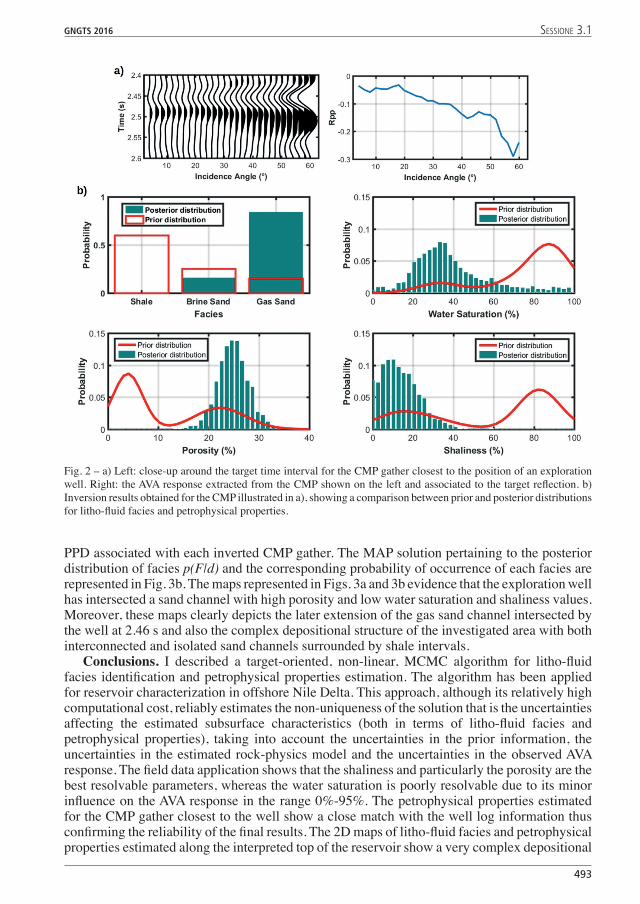
In the inversion I have considered a subset of CMP gathers extracted from the whole 3D seismic dataset and centered on the spatial location of an exploration well that reached the reservoir zone. The well log data associated to this well will be used to validate the final results. No a-priori information on the spatial correlation of petrophysical parameters has been used to constrain the inversion of adjacent CMPs. Therefore, the lateral continuity of the final results is mainly related to the lateral correlation of seismic data that is dependent on the Fresnel zone and the corresponding migration operator. A close-up of the CMP gather closest to the well location around the target interval together with the associated AVA response, are represented in Fig. 2a. This AVA response have been extracted from the negative peak amplitude of the considered reflection and normalized to the normal-incidence reflection coefficient derived from borehole logs. Note the clear class III AVA anomaly around 2.46 s that is generated by the interface separating the overlying shale from the underlying gas sand. Also note the good S/N ratio of the seismic data on the whole angle range from 0 to 60 degrees that allows me to extract a reliable AVA response over a wide-angle range. Fig. 2b shows the final results (the posterior probability distributions for both the litho-fluid facies and for the petrophysical properties of interest) obtained from the inversion of the AVA response shown in Fig. 2a. The inversion correctly attributes this AVA response to a shale-gas sand interface and the predicted petrophysical properties are in good agreement with the average petrophysical properties measured in the gas sand interval: porosity around 25%, shaliness 10% approximately and water saturation around 30-35%. From Fig. 2b emerges the higher uncertainty that characterizes the saturation estimate and conversely the good resolution on the shaliness and particularly on the porosity that reveals to be the best resolvable parameter.

The petrophysical properties estimated along the interpreted top of the reservoir are represented in Fig. 3a. This figure shows the maximum a posteriori (MAP) solution of the final

Fig. 1 – Gaussian mixture a-priori distribution for the petrophysical properties. a) A-priori distribution projected onto the Sw-φ plane and the associated marginal distributions (PDF). b) Same as a) but considering the Sw-Sh plane. Black, yellow and red colors code the shales, brine sands and gas sands, respectively.


493

PPD associated with each inverted CMP gather. The MAP solution pertaining to the posterior distribution of facies p(F|d) and the corresponding probability of occurrence of each facies are represented in Fig. 3b. The maps represented in Figs. 3a and 3b evidence that the exploration well has intersected a sand channel with high porosity and low water saturation and shaliness values. Moreover, these maps clearly depicts the later extension of the gas sand channel intersected by the well at 2.46 s and also the complex depositional structure of the investigated area with both interconnected and isolated sand channels surrounded by shale intervals.

Conclusions. I described a target-oriented, non-linear, MCMC algorithm for litho-fluid facies identification and petrophysical properties estimation. The algorithm has been applied for reservoir characterization in offshore Nile Delta. This approach, although its relatively high computational cost, reliably estimates the non-uniqueness of the solution that is the uncertainties affecting the estimated subsurface characteristics (both in terms of litho-fluid facies and petrophysical properties), taking into account the uncertainties in the prior information, the uncertainties in the estimated rock-physics model and the uncertainties in the observed AVA response. The field data application shows that the shaliness and particularly the porosity are the best resolvable parameters, whereas the water saturation is poorly resolvable due to its minor influence on the AVA response in the range 0%-95%. The petrophysical properties estimated for the CMP gather closest to the well show a close match with the well log information thus confirming the reliability of the final results. The 2D maps of litho-fluid facies and petrophysical properties estimated along the interpreted top of the reservoir show a very complex depositional

Fig. 2 – a) Left: close-up around the target time interval for the CMP gather closest to the position of an exploration well. Right: the AVA response extracted from the CMP shown on the left and associated to the target reflection. b) Inversion results obtained for the CMP illustrated in a), showing a comparison between prior and posterior distributions for litho-fluid facies and petrophysical properties.

494


Fig. 3 – a) From left to right 2D probability maps representing the maximum a posteriori solution for water saturation, porosity and shaliness, respectively, estimated along the interpreted top of the reservoir. b) Leftmost part: the maximum a posteriori solution for the litho-fluid facies distribution. Black, yellow and red correspond to shale, brine sand and gas sand, respectively. In b) the other plots represent the probability of occurrence of each facies at each CMP location. In a) and b) the white dashed crosses indicate the well location.

setting with many interconnected and isolated sand channels, surrounded by shale sequences. As a final remark I point out that the high computational cost of my MCMC algorithm (5 hours in the field data test using a i5 CPU at 2.67 GHz) can be drastically reduced by an accurate parallel implementation. Acknowledgments. The author wish to thank EDISON for making the seismic and the well log data available and for the permission to publish this work.

ReferencesAleardi M., Ciabarri F., Peruzzo F., Garcea B. and Mazzotti A. 2016: Bayesian Estimation of Reservoir Properties

by Means of Wide-angle AVA Inversion and a Petrophysical Zoeppritz Equation. In 78th EAGE Conference and Exhibition. doi: 10.3997/2214-4609.201601551.

Sambridge M. and Mosegaard K. 2002: Monte Carlo methods in geophysical inverse problems. Reviews of Geophysics, 40(3), 1-29.

Documents

a markov chain monte carLo aLgorithm for Litho-fLuid