Embed Size (px)
Citation preview
1
A Market-Based Real-Asset Martingale Valuation Approach to Optimum Inventory
Control
John A Buzacott Schulich School of Business York University Toronto ON M3J 1P3 Canada jbuzacotschulichyorkuca
Carolyn Chang Department of Finance California State University Fullerton CA 92634 cchangfullertonedu
Jack S K Chang Department of Finance and Law California State University Los Angeles CA 900 32 jskchangroadrunnercom
Key words Optimum inventory control the market-based approach Newsvendor problem real
asset martingale valuation futures contracts stochastic volatility stochastic intensity jump-
diffusion process
Please forward correspondence to
Professor Jack SK Chang 2858 Bentley Way
Diamond Bar CA 91765 Tel 1-909-860-8529 Fax 1-909-860-9819
jskchangroadrunnercom
2
A Market-Based Real-Asset Martingale Valuation Approach to Optimum Inventory
Control
ABSTRACT
We propose a novel approach to optimum inventory control by modeling a commodity traderrsquos
inventory investment as a portfolio of forward commitments taking explicit account of the
dynamics of demands costs and prices in open markets We apply the robust real-asset
martingale valuation methodology to derive a closed-form solution for the inventory value and a
simple and intuitive optimality condition Numerical analysis verifies this condition and
demonstrates that the resulting optimum policy has robust properties
3
1 Introduction
In traditional inventory theory the optimum inventory is determined by finding the optimal
reorder point and order quantity with the assumptions that costs and prices are constant and demand is
the only source of uncertainty While these assumptions are reasonable for common applications such as
the inventory management of manufactured goods service parts and many retail products they are much
less likely to be valid for the management of inventories of products that are sold in open markets like
agricultural products minerals and other commodities In open markets prices fluctuate depending on
the instantaneous balance of supply and demand So effective inventory management requires
understanding how price and demand interrelate through trading in markets This is a particular challenge
if there are many suppliers to the market and the relative size of these suppliers means that it is not
possible for a very small number of large suppliers to dominate the market and thus determine prices A
further complication is that associated with many commodity markets are futures markets where futures
contracts on commodities on traded so some market participants have the choice of participating in either
the spot or futures markets
This paper examines inventory or purchase decisions that have to be made by a participant in a
commodity market The participant could be a commodity trader deciding what contracts to enter into
with wheat farmers at planting time (although our model does not allow for harvest failure) Our approach
would also have been relevant to a late 19th century wool broker who bought wool in Australia and then
would sell it to mills in the UK and Europe after a ship voyage lasting at least 3 months Note that there
are two different but connected markets the futures market where the product is bought and the spot
market where the product is sold Product sold in the spot market is available for use immediately while
product bought in the futures market is not available for use until after some time delay When our
commodity broker buys product in the futures market he does not know the demand that he will have to
meet in the spot market During the time delay until the product is available for use he will accumulate
orders that he will meet once the product is available
4
A classic inventory model that appears to be relevant to our commodity brokerrsquos decision is the
newsvendor model The decision maker faces only uncertain demand and has to decide how much
inventory to acquire Too much and surplus inventory will have to be sold at a greatly reduced price too
little and the shortage will have to be met by acquiring additional product at a high price Since these
prices are assumed to be exogenously given by his supplier with certainty he can make the decision in
isolation from open markets Our commodity supplier however has to deal with the additional price
uncertainty that he does not know the price at which he will be able to sell the product - price will
fluctuate in open markets over the period until his product is available for delivery As such if the
supplier does not have enough inventories to meet demand he does not know how much more he will
have to pay for additional product required to meet his customersrsquo demands while if he has too much
inventory he does not know how much concession he will have to make to clear the surplus Another
complication arises from the need for our trader to finance his inventory investment Interest rates can
fluctuate over the period between making the inventory investment and realizing the cash receipts on sale
of the inventory These fluctuations in interest rates may be linked to macro economic conditions
There have been a number of attempts to expand the newsvendor framework by incorporating
certain non-stationary behaviors of the demand as well as by determining risk premiums in ways
consistent with firmrsquos objective of shareholder wealth maximization Kim and Chung (1989) Morries
and Chang (1991) and Singhal et al (1994) apply the finance theory of CAPM to factor risk premium
into valuation Stowe and Su (1997) apply the contingent-claim approach to the inventory-stocking
decision Khang and Fujiwara (2000) derive myopic optimum inventory policies under stochastic supply
Ritchken and Tapiero (1986) consider a periodic model with both stochastic demand and stochastic
purchase price and address the issue of hedging inventory in stock with futures contracts Berling and
Rosling (2005) look at the problem in a diffusion framework with stochastic demand and purchase costs
and address the issue of financial risks Cheung (1998) develops a continuous review inventory model
with a time discount to motivate customers to accept delayed deliveries and thus avoid the occurrence of
5
lost sales Flynn and Garstka (1997) consider a single-item periodic review infinite-horizon
undiscounted inventory model with stochastic demands proportional holding and shortage cost and full
backlogging Bradley and Glynn (2002) explore joint optimization of capacity and inventory in a single-
product single-station make-to-stock manufacturing system with correlated demand stream Matheus
(2000) examines the (RQ) inventory policy subject to a compound Poisson demand pattern
In this research we develop a market-based approach to value the inventory investment at the
instant when the commodity broker has to make a decision on what to order either from his supplier or in
the futures market The optimal decision will be that maximizing the value of the inventory in open
markets taking into consideration of market risk-return equilibrium To meet the task we have to develop
a model of the economy in order to determine the relationship between risk and return and we also have
to develop a model of the relationship between the futures market and the spot market for the commodity
since they are related through no-arbitrage Compared to prior newsvendor models our model is thus
unique in three ways 1) it employs a robust framework to simultaneously address the many limitations of
the prior models in terms of the non-stationary behaviors of the input and output variables their
connections as well as means to determine risk premiums 2) it is novel in viewing the inventory
investment as a portfolio of forward commitments (or futures contracts) and 3) it applies the robust real
asset martingale valuation paradigm to incorporate the market risk premiums and to drive the optimum
results in a compact way
Our paper is structured as follows in Section 2 we formally describe our decision problem and
then we briefly introduce the traditional newsvendor-type of valuation model with constant prices and
costs but uncertain and unsystematic one-period demand and discuss its shortcomings To address these
shortcomings and show why our market-based modeling approach is more general and powerful we
develop our model in Section 3 In Section 4 we use simulation to demonstrate our modelrsquos robustness in
addressing the inventory basis the discount the penalty the transaction cost the interest rate and the
clustering effects In Section 5 we offer concluding remarks and future research directions
6
2 The Basic Model and the Newsvendor Solution
A commodity trading firm orders a quantity y of a single product at time t in the whole-sale (or
futures) market at a market ordering cost of (1-u)Ft payable at the time of delivery where Ft and u
denotes respectively the equilibrium ordering cost (or futures price) and the percent discount offered
Over the interval (tt+L) the trader will receive a random number of orders D for the commodity with
commitments to deliver an agreed quantity of the product to customers at the prevailing retail (or spot)
market price of St+L at the time of delivery t+L where St+L is random with evolution determined in open
markets through supply and demand
Our trader is also assumed to be a typical small player ie a price taker but not a large supplier
ie a price setter He buys from his supplier in the whole-sale (or futures) market and sells in the spot
market to his retail customers with any imbalance disposed of only through his supplier If Dlty the
trader will have surplus inventory while if Dgty the trader will have an inventory shortfall He can not
dispose of his imbalances at the retail price in the spot market otherwise he becomes a larger player
whose action affects the retail price We assume that our trader has made prior arrangements with his
supplier to deal with surplus or shortfalls in inventory at a price that is related to the prevailing market
wholesale price or futures price Ft+L per unit at time t+L If there is excess inventory at time t+L we
assume he has entered into a short forward commitment with the supplier to instantly return the
commodity at a net salvage value equaling to Ft+L minus a penalty of q percent If there is insufficient
inventory to meet the demand we assume that he has entered into a long forward commitment with the
supplier to place an emergency order for the shortfall at a price of Ft+L plus a penalty of p percent
Obviously the presence of these costs to circumvent over-supply and -demand affect the traderrsquos
optimum inventory decision We also define the difference St ndash Ft as the inventory or forward basis and
the difference St -(1-u)Ft as the discounted inventory or forward basis where St is the initial spot price of
the commodity in the retail market Obviously the dynamic behavior of this inventory basis (basis risk)
as well as the size of u is also important considerations in the traderrsquos optimum decision For example
7
widening of the inventory basis coupled with a deeper initial purchase discount will mean more profit and
therefore the trader would order a larger quantity of inventory and vice-versa The traderrsquos decision is to
determine the optimum inventory by maximizing the net present value of this portfolio of three forward
commitments ndash a long forward commitment to purchase the commodity at a preset price a short forward
agreement to return excess inventory at a net salvage value and a long forward agreement to meet excess
demand by placing an emergency order with a penalty
Next we consider the classic newsvendor solution If demand D is the only source of uncertainty
and is unsystematic with the probability of demand D over a single period [t t+L] to be P(D) with
expected demand E(D) then the risk-adjusted discount rate is simply the market risk-free rate without the
need to incorporate a market risk premium The inventory decision at time t to decide on the ordering
decision with given purchase price (1-u)Ft and selling price St+L can thus be made in isolation from the
rest of the economy If y is ordered then the quantity (y-minDy) is surplus and we assume it can be
disposed of at a discounted price of (1-q)Ft+L However if demand is greater than y the quantity (D-
minDy) must be acquired at a penalty price of (1+p)F t+L
Then given ttLtttLt BSSBFF and where Bt denotes the current market price of a zero-
coupon unit riskless bond the net present value of the inventory position if y is ordered is
)1)()(()1)()(()1()()(1
01
y
D
t
yD
tttt FqDyDpFpyDDpFBuySDEyNPV
Note in the classical newsvendor model the purchase price is independent of L but here we have
ttLt BFF ie the purchase price Ft decreases as L increases The optimal order quantity obtained by
maximizing the NPV is then given by the y satisfying the condition
)()1(1
)(0
1
0
y
D
t
y
D
Dpqp
BupDp
A closer look at this formula however reveals that it can not really be implemented Although the
trader knows his inventory costs ie (1-u)Ft (1-q)Ft+L and (1+p)F t+L through his supplier he can not
8
really determine u q and p the sizes of the discounts or penalty without knowing Ft the equilibrium
inventory ordering cost which can only be determined in the economy To circumvent this problem we
need to generalize the newsvendor framework to allow for interactions among uncertain demand prices
and costs in open markets in ways consistent with the empirical literature We also need to develop a
proper asset pricing relation in order to incorporate market risk premiums in the valuation
To this end next we employ the robust real asset martingale valuation methodology of Schwartz
(1997) and Gibson and Schwartz (1990) in a market environment consistent with the empirical dynamics
of commodity prices and interest rate in the finance literature (eg Schwartz (1997)) - a multi-variate
Ornstein-Uhlenbeck process with stochastic interest rates and volatility augmented with a doubly
stochastic jump process We first derive a four-factor asset pricing relation in a partial equilibrium setting
by exogenously specifying a pricing kernel process with which to risk-neutralize the underlying
processes Next we determine the equilibrium inventory ordering cost in this setting as a forward price
with respect to the retail sale (output) price taking into consideration of the finance charge and the net
convenience yield (defined as benefits arising through holding inventory minus the warehouse costs)
incurred over the lead time Finally we determine the net present value of the portfolio of forward
commitments under no-arbitrage as a martingale and the corresponding optimum inventory policy by
maximizing this value
3 The Real Asset Martingale Valuation Approach
31 The Pricing Kernel Process and the Consumption-Based Jump-Diffusion Asset Pricing
Relation
We extend Schwartz (1997) to allow for jumps and stochastic arrival intensity by assuming that the
following jump-diffusion processes regarding the changes of aggregate consumption and commodity
(asset) price are exogenously given
(1) 1)()( )d(AcdZtcσdttcμtc
tdc
(2) 1)()( )dπ(Xs
dZts
dtts
SdS tt
9
where c and c and s and s denote the respective instantaneous expected value and standard-deviation
conditional on no jumps occurring for consumption change and asset return respectively and are
functions of state variables t where t denotes the information set at time t Z c and Z s denote the
standard Wiener processes with dt]tdzsdz[Eσsσσ ccsc denoting the instantaneous diffusion
covariance between asset return and consumption change is the Poisson process with stochastic
intensity parameter j representing the arrival process of consumption jump as well as asset demand A
and X denote the gross jump sizes of consumption and assert price triggered by this arrival with lnA
N(a(ωt) a(ωt)) and lnX N(x(ωt) x(ωt)) respectively and finally A and X are assumed to be
independent to Zc and Zs For ease of exposition we will denote ct as c and St as S in the remainder of the
paper We synchronize the jump arrivals of aggregate consumption and asset demand for notational
convenience otherwise the generalization is straightforward For this reason we will use the two terms
jump and demand interchangeably in the remainder of the paper
We assume that the following mean-reverting Ornstein-Uhlenbeck process governs the change of
the jump arrival intensity
(3) dZσj)dt(mκdj jjjj
where j denotes the jump arrival intensity κj the speed of adjustment mj the long-run mean rate σj2 the
instantaneous variance and Z j the standard Wiener process
The solution of this process is known to be
(4) )s(dZeeσe)m)t(j(m)v(j
v
t
sκvκ)tv(κj
ij
j
j
jj
]Tt[v
Integrating the expected value of (4) over τ yields the expected intensity over τ
(5) )τ(H]m)t(j[τm]dv)v(j[E jjjτt
t
10
where κ
e1)τ(H
j
τj
κ
j
This stochastic intensity specification addresses the clustering effect that around the time of
important news announcements the arrival intensity will be high to reflect the lumpiness of the jump
(demand) arrival but after the release of the news it will revert back to a lower long run mean level mj
and vice-versa While j itself governs the intensity of arrival the speed of adjustment parameter κj
governs the level of persistence of the intensity process ndash higher values for κj imply that the intensity
process leaves the high state more quickly and vice-versa For hedging assets (commodity assets) we
expect positive correlation between demand intensity and commodity price changes but for cyclical
assets (financial assets) that are traded in financial markets we expect the correlation to be negative to
reflect the stylized leverage effect that when volatility goes up asset price goes down
Given the aggregate consumption price dynamics and that the representative agent in the
economy exhibits a preference of the CRRA type it is well-known that eg Duffie (2001) the pricing
kernel is the agents intertemporal marginal rate of substitution ie
(6) 1)
0()
0()(
0
ct
ct
ecut
cut
et
q
where q0t is the pricing kernel defined as the state price per unit of probability or the Radon-Nikodym
derivative ct is consumption at date t θ is the time-discount factor u(ct) and u(c0) denote the marginal
utility with respect to the consumption level at time t and zero respectively and 1- is the coefficient of
relative risk aversion with lt 1 Furthermore the pricing kernel process is
(7) )dπ1(YcdZqσdtqμdqq
where θ)]ε1(2)ε1[(2cσ21))1jE(Ac(μ)ε1(qμ
cσ)ε1(qσ
AY 1ε
11
Given the specifications of the asset price the pricing kernel and the intensity shift processes it
is straightforward to derive the following consumption-based jump-diffusion asset pricing relation
THEOREM 1 Given the pricing kernel and the asset price dynamics the fundamental Euler valuation
equation dictates the following four-factor consumption-based jump-diffusion asset pricing relation
(8)
)1εAXcov()]jjm(jκj[
)1εA(E)1X(E)]jjm(jκj[scσ)ε1(rcσ)ε1(r)1X(E)]jjm(jκj[sμ
where s and )( jmj jj denotes the instantaneous expected diffusion return and jump arrival
intensity respectively E is the expected value operator and X the gross spot jump size r is the
instantaneous riskless rate (1-) the CRRA measure dt]tdzdz[Eσσσ crcrrc the instantaneous
diffusion covariance between interest rate and consumption change dt]tdzsdz[Esσsσσ csc the
instantaneous diffusion covariance between asset return and the consumption change and A is the gross
consumption jump size
Proof of Theorem 1 See Appendix
Equation (8) stipulates that the asset risk premium has four components two diffusion risk
premiums
- rcε)σ1( and scε)σ1( and two jump risk premiums )1ε)E(A1E(X)]jm(κj[ jj which
compensates for the jump arrival uncertainty and )1εA(Xcov)]jm(κj[ jj which compensates
for the jump size uncertainty Since σrclt0 because when interest rates go up consumptions go down and
1-ε gt0 because of risk-aversion the interest rate risk premium is negative Since the leverage effect
dictates that 0)dZσ1εXAcov( jj all other risk premiums are positive for cyclical assets (financial
assets) and negative for hedging assets (commodity assets) When j is deterministic both the interest rate
and the intensity risk premiums shrink to zero and consequently Eq (8) shrinks to Changrsquos (1995) three-
12
factor jump-diffusion asset pricing relation Furthermore when j is zero with no jump arrival Eq (8)
shrinks to the one-factor diffusion asset pricing relation of Breeden (1979) and Ross (1989) Finally
when the asset price jump size is deterministic ie )1ε(XAcov = 0 the bearing of jump arrival
uncertainty and jump intensity uncertainty must still be rewarded
Next given θ)]ε1(2)ε1[(2cσ21]))1jE(Acμ)[ε1(qμ and
1 AY it is
straightforward to show that applying the fundamental Euler valuation equation to a riskless asset yields
jυυ
)1εE(A)jmκj(rcσ)ε1(qμr
21
j(j
(9)
where
])1E(A)ε1()1εE(A)κ1[(υ
)1εE(Amκθ)]ε1(2)ε1[(2cσ21)rcσcμ)(ε1(υ
j2
jj1
(11)
and (10)
which indicates that in our economy uncertainty regarding jump (demand) arrival intensity induces
stochastic interest rates Since both qμ- and 1-ε are positive but σrc is negative Eq (9) reveals that the
faster the diffusion mean of the pricing standard attenuates the smaller the covariance between interest
rate and consumption changes is the faster demand arrives and the larger the expected consumption
jump size is the higher is the interest rate Furthermore since r is linear in j an application of the
generalized Itorsquos lemma to Eq (3) of r with respect to j and t leads to the following induced
mean-reverting Ornstein-Uhlenbeck interest rate process
(12) dZσr)dt(mκdr jrrr
where jr
j21r mυυm 2jr
and jcrc ρρ
Eq (12) offers a trade-arrival interpretation of stochastic interest rates based upon the notion that
demand or trade-arrival is what generates interest rates with Eq (9) offering the equilibrium supports to
such a relation ndash aggregate consumption embeds a jump component CRRA and jump arrival intensity
13
follows a mean-reverting Ornstein-Uhlenbeck process Replacing the interest rate risk premium with the
intensity risk premium further condenses Eq (8) to
)1εAXcov()]jm(κj[
)1εA(E)1X(E)]jm(κj[σ)ε1(συ)ε1(r)1X(E)]jm(κj[μ
jj
jj2jjs scjc
(13)
Next note that in our doubly-stochastic jump-diffusion specification the total instantaneous
variances of consumption change and asset return are 2ajj
2c σ)]jm(κj[σ and
σ)]jm(κj[σ 2xjj
2s respectively Since these variances are linear in j as in the case of r by
Itorsquos lemma they should also follow mean-reverting Ornstein-Uhlenbeck processes Again this is because
in our setting trade arrival is the underlying latent variable that generates volatility ie a trade-arrival
interpretation of stochastic volatility in the spirit of Andersen (1996) In sum the above derivations show
that our approach of modeling stochastic intensity in a doubly-stochastic jump-diffusion framework is an
internally consistent and parsimonious way to simultaneously consider stochastic interest rates stochastic
volatility and jumps with random heights and arrival intensity
32 The Inventory Investment Problem
In our model of the small trader the experienced demand will be a thinning of the process of
jump arrivals in the model of the economy The total number of jump arrivals during a period of length L
is the total demand that must be met at the end of the period At the beginning of the period the trading
firm must choose an optimum order quantity y with lead time of a single-period of L so as to bring the
total initial position (IP = rp + y where rp denotes on-hand inventory) to an optimum level of IP for
covering the forthcoming periodrsquos stochastic demand At the end of the period the trading firm will
liquidate excess inventory Since on-hand inventory is a given constant we can effectively assume it
away without sacrificing the generality of the model In this sense y and IP are used interchangeably
We assume the inventory is replenished from an outside supplier with ample supply and the initial
14
inventory ordering cost quoted by this supplier is lower than its benchmark equilibrium value An instant
refill from the supplier to meet an excess demand incurs a penalty An instant return to the supplier to
liquidate an excess inventory incurs a discount to arrive at the net salvage value
Effectively in this setting the firm undertakes a long forward position by placing the inventory
order at the beginning of the period to purchase the commodity from the supplier at a preset forward
(purchase) price of (1-u)Ft with a maturity of L where u denotes the percentage discount In order to
meet excess demand at the end of the period the firm also enters into a long forward agreement to
purchase the commodity from the supplier as an instant refill at a price of LtFp )1( where LtF is the
prevailing equilibrium ordering cost and 1+p is a preset penalty ratio In order to liquidate excess
inventory at the end of the period the firm also enters into a short forward agreement to instantly return
the surplus commodity back to the supplier at a price of LtFq )1( where (1-q) is a preset cost ratio
33 Determining the Equilibrium Purchase Price as a Forward Price in the Real Asset Martingale
Framework
Since by placing an order with a preset purchase price and lead time a trader essentially enters in
a long forward position in the rest of the paper we will use the two terms purchase price and forward
price and the two terms sale price and spot price interchangeably By the same token a backorder
resembles a short forward position Since the spot price as well as the financing charge change
stochastically in our modeling we should also expect the purchase price to be stochastic
Past literature eg Moinzadeh (1997) Golabi (1985) and Kalymon (1971) have exogenously
specified the stochastic purchase prices according to certain processes In this study we undertake a new
and novel approach by endogenizing the stochastic purchase price based upon the seminal cost-of-carry
forward pricing concept to link pricing in the input market to pricing in output market Assuming that all
participants in the market experience the same lead time L the seminal cost-of-carry concept in forward
pricing dictates that under no-arbitrage the purchase price must equal the total cost of carrying the spot
commodity over lead-time L These costs include the spot price and holding costs (financing and
15
warehouse costs) and also what we term ldquoconvenience yieldsrdquo which are benefits arising through
holding inventory They stem from two possible sources 1) any flow of cost saving accruing to the firm
from the supplier but not to the firmrsquos customers such as discounts on purchases and 2) the flow of
services accruing only to the holder of the spot commodity such as short term yields that can be earned by
lending the physical inventory out to arbitrageurs and others In this context the convenience yields are
the ldquoprofitsrdquo that the commodity trader earns while holding costs are the ldquocostsrdquo the trader incurs through
embarking on the inventory investment We define basis as spot price minus purchase price Obviously
the basis becomes positive if convenience yields dominate but negative when inventory holding costs
dominate The dynamic behavior of the basis ie basis risk is thus dictated by the net change of these
two factors over time
Let i to be the marginal net rate of convenience yield defined as total convenience yield minus
warehouse cost Should this rate and the financing rate be constant we would have the familiar cost of
carry formula that eSF L)ir(tt
In our dynamic setting however we price the forward contract as
martingale by assuming that i follows a mean-reverting Ornstein-Uhlenbeck process This means that any
current basis whether positive or negative will revert back to its long-run mean at a given speed of
adjustment
(14) idZiσi)dti(miκdi
where i is the net convenience yield rate κi denotes the speed of adjustment mi the long-run mean rate
σi2 the instantaneous variance and Z i the standard Wiener process Further let dtρ)dZdZcov( siis
where siρ denotes the correlation coefficient
The presence of convenience yield means that the spot commodity can be treated as an asset that
pays a stochastic dividend yield i Since jump risk convenience yield risk as well as intensity risk can
not be hedged the risk-neutralized processes for the three factors according to (13) should be
(15) dπ)1X(sdZsσdt))1X(E)1εA(E)]jm(κj[ir(dSS jj
16
(16) idZiσdt]iσiλi)i(miκ[di
(17) dZσdt]σλr)(mκ[dr jrrrrr
where )1εA(E)]jm(κj[ jj is the risk-adjusted jump arrival intensity
πd is the corresponding
Poisson process X is the risk-adjusted gross jump size with xx σ)AlnXln(covε)1(μN~Xln
and ci σρ)ε1(λ ic and cjcr σρ)ε1(λ are the respective convenience yield and diffusion risk
premiums
Under no-arbitrage and with tB a zero-coupon unit bond with matching maturity L being the
numeraire the martingale valuation principal dictates that the normalized forward price must equal to the
expected future spot price with respect to the risk-neutralized processes (15) - (17)
(18) B
1e)L(AS)LttiS(F
t
ti)L(
iH
ttt
4
)2)((exp)(
22
2
22
i
ii
i
iissiiiiiiii HmLHLA
1
)(i
Li
i
eLH
where tB according to Vasicek (1977) is
(19) etB)r(rp
rκ]2)2)L(
r(kH[L))L(
rk(H
]m))[R((rp)(rpmk)L
e(H rrrrrrrrrrrr
Lr
222)( 21)( 2)(1 where
and p(r) and )R(infin denote respectively the market price of risk and the bondrsquos limiting yield
Close examination of (18) reveals that the jump components have disappeared This happens
because the occurrence of jumps only causes the distribution of the spot price to be more skewed and
kurtotic than the log-normal it does not affect the risk-neutralized expectation that is based upon the
entire distribution
17
To determine the risk-neutralized forward price process let us assume the forward price function
)( LttriSF ttt is twice continuously differentiable in S i and r Then applying generalized Itorsquos
lemma to )( LttriSF ttt with respect to the risk-neutralized processes for the three factors gives the
risk-neutralized process for forward price change
where
)()(2 )(2)(22
)(22
)(222
rH
iH
riirrH
srrsiH
siisrH
riH
isf (21)
)(
f
srrrsiiissf
HH
(22)
where i
i
i
eH
1
)( and 1
)(r
r
r
eH
f denotes the forward returnrsquos instantaneous standard-
deviation and ρsf denotes the correlation coefficient between spot return and forward return the Poisson
process dπ and random gross jump size X are the same as in the spot price process because the Poisson
event for the forward price occurs if and only if the Poisson event for the spot price occurs Moreover
when the Poisson event occurs the jump in the forward price should be equal to the jump in the spot price
given the former is linear in the latter
34 Risk-Neutral Valuation of the Inventory as a Portfolio of Forward Commitments in the Real
Asset Martingale Framework
For simplicity we assume that demand arrival intensity and asset price revision are uncorrelated
in our risk-neutral world The firm will meet the end-of-period demand at a cost of (1-u)Ft up to the order
quantity Excess inventory will be liquidated at a price of (1-q)Ft+ L and excess demand will be met by
placing an emergency order at a penalty cost (1+p)Ft+L where q and p are transaction cost and penalty
ratios respectively The expected end-of-period payoff conditional on an initial inventory position y is
)1())1()1()]([( (20) dXf
dZf
dtXEAEjmjrFdF jj
18
~
1()~
)1()~
)1()~
)1()~
(23)
1yD
)]Lt
Fp)E(Lt
Sy)[E((D]t
FLt
S[E(E[j(L)])yP(D
]t
FLt
Fc)E(-D)[(1(y]t
FLt
S[E(y
0D
E[j(L)])DP(D E(y)
u
uu
where P() is the Poisson pdf E[j(L)] is the risk-adjusted expected demand arrival intensity over L ie
E[j(L)] = )1
A(E)L(jH]jm)t(j[Ljm
ε with )
1A(E
ε being the risk-adjustment factor and per Eqs
(15) and (20) the risk-neutralized spot and forward price changes over L are respectively
2x
DL2s
A)]lnXln(cov)1(x
[DL]2s
)21()1X(E)1A(E)]jj
m(j
j[ir[N~t
SLt
S~
ln σσεμσεκ
and
2x
DL2f
A)]lnXln(cov)1(x
[DL]2f
)21()1X(E)1A(E)]jj
m(j
j[r[N~t
FLt
F~
ln σσεμσεκ
Under no-arbitrage and with tB being the numeraire the martingale valuation principal dictates
that the normalized net present value of the initial inventory position must equal to the expected value of
its end-of-period payoff with respect to the risk-neutralized demand uncertainty and price processes ie
NPV(y) tB = E(y) Since in this risk-neutral world t
B)~
tB
tS
)~ t
F
LtFE( LtSE( =+=+ and upon substitution
and simplification we derive the NPV of the initial position as a function of the order quantity y as
]
1
))])(([()]1( )1[(
))1(1())1()](([)(
yD
yDLjEDΡt
Fpt
Bu
tFu
tBq
tF
tBu
tSLjEyNPV D)(y
y
0D
E[j(L)])P(D(24)
This expression dictates that in our risk-neutral world the present value of the inventory
investment as a portfolio of forward commitments is composed of three terms the first value stems from
the expected cash inflow due to the initial under-pricing the second value stems from the expected cash
flow due to excess inventory and the third value stems from the expected cash flow due to excess
demand
Next examining the difference between NPV(y) and NPV(y+1) leads to
19
0 1
)]))([())1()1(()])([())1(1((()()1( (25)
y
D yDLjEDPptBuLjEDPutBqtFyNPVyNPV
This difference is negative if
)1()1(0
)])([()( (26) ptBuy
DLjEDPpq
Similarly 0)1y(NPV)y(NPV if )1()1()])([()(0
pBuLjEDPpq t
y
D
Hence y is optimal if
1
0)])([(
0
)1(1)])([( (27)
y
DLjEDP
y
D qp
tBupLjEDP
where note that E[j(L)] is the risk-adjusted expected demand arrival intensity over L Note however that
if 1)1(1
qp
Bup t ie if tBuq )1()1( then the optimal y is the maximum possible demand
bounded by the traderrsquos available investment capital
To summarize we have developed a market-based optimum inventory control model that works
in the real world with risk-averse investors explicitly incorporates the stylized dynamics of prices costs
and demands and explicitly determines the equilibrium inventory ordering cost and market discount It is
straightforward to show that our valuation formula (Eq (24)) and optimality condition (Eq (27) collapse
onto the corresponding results in the traditional newsvendor solution where demand is the only source of
uncertainty as derived in Section 2 under 1) risk-neutrality 2) constant demand arrival intensity 3)
constant interest rates and 4) exogenously given equilibrium inventory ordering cost and market
discount
Since according to Eq (18) tB
1ti)L(
iH
e)L(AtS)LtttitS(F
we can further condense Eq
(24) to become a function of the initial spot price as
20
PV (28)
1yDtt
y
0Dttt
)yD)])(L(j[ED(Ρ]B
)p1(u)-[(1S
D)(yE[j(L)])P(D)]u1(B
c1[S)]L(j[ES)y(N
ti)L(iHe)L(A
ti)L(iHe)L(A]ti)L(iH
e)L(A)u1(1[
This expression subsumes the equilibrium inventory order cost and relates the NPV of the
inventory investment directly to the spot price and the net cost of carrying the spot commodity among
others
35 Estimation and Calibration of the Model Parameters
We need to estimate a number of jump parameters in our model but it is well known that direct
estimation of these parameters is difficult to gain great precision Theoretically since the probability
density function corresponding to the jump-diffusion process is known we can estimate jump parameters
by using the maximum likelihood approach with time-series data as illustrated in Jorion (1988) However
in actual implementation two issues need to be addressed first it requires a very long time series of spot
price to capture actual random and sporadic occurrences of jumps and second since the jump arrival
intensity may change substantially over a long period of time reverting between low and high state it is
necessary to estimate jointly the spot price and the intensity shift processes To this end Eraker (2000)
has recently developed an alternative Markov chain Monte Carlo based approach that treats jumps as an
additional state variable making it convenient to draw inferences about jump occurrences
Alternatively one can calibrate the jump and mean-reversion parameters to traded market prices
For example Hillard and Reis (1999) imply jump parameters from traded option prices in their study of
commodity futures option pricing Pan (2002) implies jump risk premia from a joint time series of the
SampP 500 index and near-the-money short-dated option prices In the real option literature it is also
common to calibrate the commodity process parameters to the traded commodity futures and option
prices
21
4 Numerical Validation
We demonstrate optimization and verify the modelrsquos predictions numerically We first examine the
inventory basis effect the discount effect the penalty effect the transactions cost effect the interest rate
effect and then take a close look at clustering by examining the impacts of the mean-reverting behavior
of the trade arrival intensity We select the following parameter values for the common factors L = 1 m
= 10 S = 100 02021)1
A(E ε where L denotes the number of time period m denotes the long-run
demand arrival intensity per period S denotes the current sale price of the commodity and )1
A(Eε
denotes the risk-adjustment factor for the expected demand arrival density This value of 10202 is within
the range of that of an average risk-averse investor per Jorion (1988) and Friend and Blume (1975)
Since the larger the basis (the difference between the current sale price of the commodity and the
current purchase price or ordering cost of the inventory) the lower the initial purchase price of the
inventory we would expect the inventory value to be a positive function of the inventory basis However
since we fix the initial discount we should expect the optimum order quantity to be a constant Table 1
below reports the numerical result when the basis is allowed to increase from zero to 20 percent of the
sale price of the commodity With the initial demand arrival intensity at its long-run mean of 10 units per
period speed of adjustment at 5 units per period discount at 02 transaction cost at 03 penalty at 02
and bond price at 09 the optimum order quantity is 16 units and the corresponding inventory value
increase from 270794 to 420675 These results are consistent with the predictions
______________________________
Insert Table 1 About Here
______________________________
Next we look at the discount effect The prediction is that the larger the discount the more the
firm should order and thus the larger should be the inventory value Table 2 below reports the numerical
result when the discount increases from zero to 05 With the initial demand arrival intensity at its long-
run mean of 10 units per period speed of adjustment at 5 units per period basis at zero transaction cost at
22
03 penalty at 02 and bond price at 09 the optimum order quantity increases from 11 units to above 30
units and the corresponding inventory value increases from 400141 to above 105606 These results are
consistent with the predictions
______________________________
Insert Table 2 About Here
______________________________
Next we should also expect that 1) the larger the penalty ratio the larger the optimum order
quantity to prevent stock-outs and the smaller the initial inventory value to reflect the more severe
penalty and 2) the larger the transaction cost the lower the optimum order quantity to prevent excess
inventory and thus the smaller the inventory value to reflect the larger transaction cost when excess
inventory are returned and 3) the higher the bond price the higher the present value of the purchase price
of the inventory and thus the lower the optimum order quantity and the corresponding initial inventory
value Table 3 below reports the numerical results regarding the penalty effect with the penalty
increasing from 0 to 10 The results show that with the initial demand intensity at its long-run mean rate
of 10 units per period speed of adjustment at 5 units per period basis at zero discount at 02 transaction
cost at 03 and bond price at 09 the optimum order quantity and its corresponding inventory value
increases from above 15 units to 18 units and decreases from 272417 to 267905 respectively These
results are consistent with the predictions
______________________________
Insert Table 3 About Here
______________________________
Table 4 below reports the numerical results regarding the transaction cost effect with the cost
increasing from 0 to 05 The results show that with the initial demand intensity at its long-run mean rate
of 10 units per period speed of adjustment at 5 units per period basis at zero discount at 02 penalty at
02 and bond price at 09 the optimum order quantity and its corresponding inventory value decreases
23
from above 30 units to 12 units and from above 840 to 204485 respectively These results are consistent
with the predictions
______________________________
Insert Table 4 About Here
______________________________
Table 5 below reports the results regarding the interest rate effect with the bond price increasing
from 08 to 10 The results show that with the initial demand intensity at its long-run mean rate of 10
units per period speed of adjustment at 5 units per period basis at 10 units discount at 02 transaction
cost at 03 and penalty at 12 the optimum order quantity and its corresponding inventory value
decreases from above 30 units to 13 units and from above 48606 to 157733 respectively These results
are consistent with the predictions
______________________________
Insert Table 5 About Here
______________________________
Finally we take a close look at the impacts of clustering With the long-run demand arrival
intensity at 10 units per period basis at 10 penalty ratio at 12 and the bond price at 09 we consider two
scenarios when the initial intensity is low at 5 units and high at 15 units In each scenario we vary the
speed of adjustment toward the mean from 2 to 10 units per period Table 6 below reports the results As
the speed of adjustment increases clustering weakens and mean-reversion toward the mean strengthens
which leads to increased expected demand intensity when the initial intensity is low and decreased
expected demand intensity when the initial intensity is high Consequently the optimum inventory level
jumps up from 13 units to 15 units and down from 19 units to 17 units respectively with the
corresponding value of the initial inventory increasing from 269515 to 327995 and decreasing from
422073 to 363349 respectively These results are also consistent with the predictions
24
______________________________
Insert Table 6 About Here
______________________________
To summarize we have found that 1) the lower the net carrying cost and the larger the initial
discount the higher is the initial inventory value and thus the more the firm should order 2) the larger the
penalty ratio the larger should be the initial inventory to prevent from stock-outs but the smaller is the
initial inventory value to reflect the more severe penalty 3) the larger the discount in determining the net
salvage value the lower the optimum order quantity to prevent excess inventory and thus the smaller the
initial inventory value 4) the higher the bond price the higher the present value of the purchase price of
the inventory and thus the lower the optimum order quantity and the initial inventory value and 5) in the
clustering effects when the initial demand arrival intensity is low as the speed of adjustment increases
clustering weakens and mean-reversion toward the higher mean strengthens leading to increased
expected demand intensity Consequently the optimum inventory level jumps up with the corresponding
value of the initial inventory increasing to reflect the increased expected demand Conversely when the
initial demand arrival intensity is high the opposite happens
5 Conclusions
We have modeled a commodity traderrsquos inventory as a portfolio of forward contracts in open
markets by using the real asset martingale valuation methodology with the market risk premiums attained
in an internally consistent jump-diffusion stochastic interest rates and stochastic volatility economy
where the underlying trade arrival intensity serves as the latent stochastic factor Optimum inventory
control is implemented by shareholdersrsquo wealth maximization with respect to the inventory decision
variables leading to a simple and intuitive optimality condition and a closed-form solution for the
inventory value Numerical analysis demonstrates that the resulting optimum policy has robust
properties In comparison to the traditional approach the contribution of our model is three-fold 1) it
works in the real world but the traditional model only works in the risk-neutral world 2) it explicitly
25
incorporates the stylized dynamics of prices costs and demands but the traditional model only allows for
demand uncertainty and 3) it shows how to endogenize the inventory ordering cost but this cost is not
known in the traditional model
This new and novel real asset approach can be further generalized to a multi-period dynamic
control setting with inclusion of commodity futures trading to further fine-tune the topology contour
Applications to other operational management problems such as capacity expansion and supply chain are
also potential topics It will be informative to examine empirically how the optimum inventory decision
varies across different commodities with particular characteristics eg gold that is more sensitive to
interest rate shocks vs oil that is more sensitive to clustering It will also be informative to examine how
the size of a demand shock and the current level of inventory jointly impact the model It is conceivable
that a large positive demand shock when inventories are high would produce a different decision than
when inventories are low ndash the decision should be time varying and partly driven by business cycles
References Andersen TG 1996 Return volatility and trading volume An information flow interpretation of
stochastic volatility Journal of Finance 51 169-204
Berling P K Rosling 2005 The effects of financial risks on inventory policy Management Science 51
1804-1815
Bradley JR PWGlynn 2002 Managing capacity and inventory jointly in manufacturing systems
Management Science 48 273-284
Breeden DT 1979 An intertemporal asset pricing model with stochastic consumption and investment
opportunities Journal of Financial Economics 7 265-296
Chang C 1995 A no-arbitrage martingale analysis for jump-diffusion valuation Journal of Financial
Research 17 351-381
Cheung KL 1998 A continuous review inventory model with a time discount IIE Transactions 30 747-
757
26
Duffie D 2001 Dynamic Asset Pricing Theory Third Edition Princeton University Press
Eraker B 2000 Do stock prices and volatility jump Reconciling evidence from spot and option prices
Working Paper Graduate School of Business University of Chicago
Flynn J S Garstka 1997 The optimum review period in a dynamic inventory model Operations
Research 45 736-750
Friend I N Blume 1975 The demand for risk assets American Economic Review 900-922
Golabi K 1985 Optimum inventory policies when ordering prices are random Operations Research 33
575-588
Gibson R ES Schwartz 1990 Stochastic convenience yield and the pricing of oil contingent claims
Journal of Finance 45 959-976
Hilliard JE J Reis 1998 Valuation of commodity futures and options under stochastic convenience
yields interest rates and jump diffusions in the spot Journal of Financial and Quantitative Analysis
33 61-85
Hilliard JE J Reis 1999 Jump processes in commodity futures prices and options pricing American
Journal of Agricultural Economics 81 273-286
Harrison JM DM Kreps 1979 Martingale and arbitrage in multiperiod securities markets Journal of
Economic Theory 20 381-408
Harrison JM SR Pliska 1981 Martingale and stochastic integrals in the theory of continuous trading
Stochastic Processes and Their Applications 11 215-260
Jorion P 1988 On jump processes in the foreign exchange and stock markets Review of Financial
Studies 1 427-446
Kalymon BA 1971 Stochastic prices in a single-item inventory purchasing model Operations Research
19 1434-1458
Khang DB O Fujiwara 2000 Optimality of myopic ordering policies for inventory model with
stochastic supply Operations Research 48 181-196
27
Kim Y K Chung 1989 Inventory management under uncertainty A financial theory for the
transactions motive Management and Decision Economics 6 292-298
Matheus P L Gelders 2000 The (RQ) inventory policy subject to a compound Poisson demand
pattern International Journal of Production Economics 68 307-320
Moinzadeh K 1997 Replenishment and stocking policies for inventory systems with random deal
offering Management Science 43 334-342
Morris JR JSK Chang 1991 Inventory policies in the CAPM valuation framework Advances In
Working Capital Management 2 227-239
Pan J 2002 The jump-risk premia implicit in options evidence from an integrated time-series study
Journal of Financial Economics 63 3-50
Ritchken P C Tapiero 1986 Contingent claims contracting for purchasing decisions in inventory
management Operations Research 34 864-70
Ross S 1989 Information and volatility the no-arbitrage martingale approach to timing and resolution
irrelevancy Journal of Finance 44 1-17
Rubinstein M 1976 The valuation of uncertain income streams and the valuation of options Bell
Journal of Economics and Management Science 7 407-425
Schwartz ES 1997 The stochastic behavior of commodity prices implications for valuation and
hedging Journal of Finance 52 922-973
Singhal VR AS Raturi J Bryant 1994 On incorporating business risk into continuous review
inventory models European Journal of Operational Research 75 136-150
Stowe JD T Su 1997 A contingent-claims approach to the inventory-stocking decision Financial
Management 26 42-55
Vasicek O 1977 An equilibrium characterization of the term structure Journal of Financial Economics
5 177-188
28
Table 1 The Basis Effect
Parameters
L = 10 κ = 50 m = 100 j = 100 u = 02 p = 02 c = 03 B = 090 S = 1000
Table 1 below reports the numerical result when the inventory ordering cost is allowed to decrease from
100 to 80 With the initial demand arrival intensity at its long-run mean of 10 unit per period speed of
adjustment at 5 units per period bond price at 09 discount at 02 penalty at 02 and transaction cost at
03 the optimum order quantity is 16 units and the corresponding inventory value increase from 270794
to 420675
-300
-200
-100
0
100
200
300
400
500
0 10 20 30
Order Quantity
Inv
en
tory
Va
lue
S-F=20
S-F=16S-F=12S-F=8S-F=4
S-F=0
29
Table 2 The Discount Effect
Parameters
L = 10 κ = 50m = 100j = 100p = 02c = 03B = 09S = 1000F = 1000
Table 2 below reports the numerical results regarding the discount effect with the discount increasing
from 0 to 05 The results show that with the initial demand intensity at its long-run mean rate of 10 units
per period speed of adjustment at 5 units per period basis at zero bond price at 09 penalty at 02 and
transaction cost at 03 the optimum order quantity and its corresponding inventory value increases from
11 units to above 30 units and from 400141 to above 105606 respectively
-400
-200
0
200
400
600
800
1000
1200
0 10 20 30
Order Quantity
Inv
en
tory
Va
lue
u=0
u=01
u=02
u=03
u=04
u=05
30
Table 3 The Penalty Effect
Parameters
L = 10 κ = 50m = 100j = 100u=02c=03B = 09S = 1000F = 1000
Table 3 below reports the numerical results regarding the penalty effect with the penalty increasing from
0 to 1 The results show that with the initial demand intensity at its long-run mean rate of 10 units per
period speed of adjustment at 5 units per period basis at zero bond price at 09 discount at 02 and
transaction cost at 03 the optimum order quantity and its corresponding inventory value increases from
15 units to 18 units and decreases from 272417 to 267905 respectively
-400
-300
-200
-100
0
100
200
300
400
0 10 20 30
Order Quantity
Inv
en
tory
Va
lue
p=02
p=04
p=06 p=08p=1
p=0
31
Table 4 The Transaction Cost Effect
Parameters
L = 10 κ = 50m = 100j = 100 u=02 p=02B = 09S = 1000F = 1000
Table 4 below reports the numerical results regarding the transaction cost effect with the cost increasing
from 0 to 05 The results show that with the initial demand intensity at its long-run mean rate of 10 units
per period speed of adjustment at 5 units per period basis at zero bond price at 09 discount at 02 and
penalty at 02 the optimum order quantity and its corresponding inventory value decreases from above 30
units to 12units and from above 840 to 224485 respectively
-400
-200
0
200
400
600
800
1000
0 5 10 15 20 25 30
Order Quantity
Inv
en
tory
Va
lue q=01
q=02
q=03
q=04
q=05
q=0
32
Table 5 The Interest Rate Effect
Parameters
L = 10 κ = 50m = 100j = 100 u=02p = 02c = 03S = 1000F = 900
Table 5 below reports the results regarding the interest rate effect with the bond price increasing from 08
to 10 The results show that with the initial demand intensity at its long-run mean rate of 10 units per
period speed of adjustment at 5 units per period basis at 10 units discount at 02 transaction cost at 03
and penalty at 02 the optimum initial inventory position and its corresponding inventory value decreases
from above 30 units to 13 units and from above 48606 to 157733 respectively
-300
-200
-100
0
100
200
300
400
500
600
0 5 10 15 20 25 30
Order Quantity
Inv
en
tory
Va
lue
B=08
B=084
B=088
B=092
B=096
B=1
33
Table 6 The Clustering Effects
Parameters
L = 10m = 100j = 50 and 150p = 12B = 090S = 1000F= 900
We take a close look at the impacts of clustering with high and low initial intensities by varying the speed
of adjustment toward the mean ( κ ) from 2 to 10 units per period As this speed increase clustering
weakens and mean-reversion toward the mean strengthens which leads to increased expected demand
intensity when the initial intensity is low and decreased expected demand intensity when the initial
intensity is high Consequently the optimum inventory level jumps up from 13 units to 15 units and
down from 19 units to 17 units respectively with the corresponding value of the initial inventory
increasing from 269515 to 327995 and decreasing from 422073 to 363349 respectively
0
50
100
150
200
250
300
350
400
450
0 5 10 15 20
Order Quantity
Inv
en
tory
Va
lue
κ=2
κ=4
κ=2
κ=8
κ=4
κ=8
Low initial
demand
High initial
demand
34
Appendix Proof of Theorem 1
THEOREM 1 Given the pricing kernel and the asset price dynamics the fundamental Euler valuation
equation dictates the following four-factor consumption-based jump-diffusion asset pricing relation
(8)
)1AXcov()]jjm(jj[
)1A(E)1X(E)]jjm(jj[sc)1(rc)1(r)1X(E)]jjm(jj[s
εκ
εκσεσεκμ
where s and )( jmj jj denotes the instantaneous expected diffusion return and jump arrival
intensity respectively E is the expected value operator and X the gross spot jump size r is the
instantaneous riskless rate (1-) the CRRA measure dt]tdzdz[E crcrrc σσσ the instantaneous
diffusion covariance between interest rate and consumption change dt]tdzsdz[Ess csc σσσ the
instantaneous diffusion covariance between asset return and the consumption change and A is the gross
consumption jump size
Proof of Theorem 1
Applying the generalized Itos lemma to the pricing-kernel-scaled spot price qs we obtain
(A2-1) )1()()( dXYdZcdZqdtqqsqsd sssqs
where jjjj dZj)dt(mdj σκ and dt]tqdzsdz[Eqssq σσσ is the instantaneous diffusion
covariance between spot return and pricing kernel change
Applying the fundamental Euler valuation equation that E[d(qs)qs] = 0 to (A2-1) by taking the
expectation of (A2-1) we obtain
(A2-2) )dtdZXYcov()1E(XY)dtdjj(Esqqμs jjσσμ
where )jm(j)dtdjj(E jj κ denotes the instantaneous expected jump arrival intensity
Applying this equation to a riskless fund that continuously earns an instantaneous riskless return r
whose change follows a diffusion process yields
(A2-3) )1E(Y)dtdjj(Erqqμr σ
35
where dt]tqdzdz[Eqrq rr σσσ is the instantaneous diffusion covariance between the interest rate
and the pricing kernel change and Y Aε-1
because of the CRRA preference assumption
Recall from Eq (7) cσ)1(qσ ε and thus with this substitution
(A2-4) dtscε)σ1(dt]tsdzcdz[Esσcε)σ1(dtsqσ and
(A2-5) dtrcε)σ1(dt]tdzcdz[Eσε)σ1(dtrqσ rrc
Finally substituting (A2-3) - (A2-5) into (A2-2) and rearranging yields Theorem 1
QED
2
A Market-Based Real-Asset Martingale Valuation Approach to Optimum Inventory
Control
ABSTRACT
We propose a novel approach to optimum inventory control by modeling a commodity traderrsquos
inventory investment as a portfolio of forward commitments taking explicit account of the
dynamics of demands costs and prices in open markets We apply the robust real-asset
martingale valuation methodology to derive a closed-form solution for the inventory value and a
simple and intuitive optimality condition Numerical analysis verifies this condition and
demonstrates that the resulting optimum policy has robust properties
3
1 Introduction
In traditional inventory theory the optimum inventory is determined by finding the optimal
reorder point and order quantity with the assumptions that costs and prices are constant and demand is
the only source of uncertainty While these assumptions are reasonable for common applications such as
the inventory management of manufactured goods service parts and many retail products they are much
less likely to be valid for the management of inventories of products that are sold in open markets like
agricultural products minerals and other commodities In open markets prices fluctuate depending on
the instantaneous balance of supply and demand So effective inventory management requires
understanding how price and demand interrelate through trading in markets This is a particular challenge
if there are many suppliers to the market and the relative size of these suppliers means that it is not
possible for a very small number of large suppliers to dominate the market and thus determine prices A
further complication is that associated with many commodity markets are futures markets where futures
contracts on commodities on traded so some market participants have the choice of participating in either
the spot or futures markets
This paper examines inventory or purchase decisions that have to be made by a participant in a
commodity market The participant could be a commodity trader deciding what contracts to enter into
with wheat farmers at planting time (although our model does not allow for harvest failure) Our approach
would also have been relevant to a late 19th century wool broker who bought wool in Australia and then
would sell it to mills in the UK and Europe after a ship voyage lasting at least 3 months Note that there
are two different but connected markets the futures market where the product is bought and the spot
market where the product is sold Product sold in the spot market is available for use immediately while
product bought in the futures market is not available for use until after some time delay When our
commodity broker buys product in the futures market he does not know the demand that he will have to
meet in the spot market During the time delay until the product is available for use he will accumulate
orders that he will meet once the product is available
4
A classic inventory model that appears to be relevant to our commodity brokerrsquos decision is the
newsvendor model The decision maker faces only uncertain demand and has to decide how much
inventory to acquire Too much and surplus inventory will have to be sold at a greatly reduced price too
little and the shortage will have to be met by acquiring additional product at a high price Since these
prices are assumed to be exogenously given by his supplier with certainty he can make the decision in
isolation from open markets Our commodity supplier however has to deal with the additional price
uncertainty that he does not know the price at which he will be able to sell the product - price will
fluctuate in open markets over the period until his product is available for delivery As such if the
supplier does not have enough inventories to meet demand he does not know how much more he will
have to pay for additional product required to meet his customersrsquo demands while if he has too much
inventory he does not know how much concession he will have to make to clear the surplus Another
complication arises from the need for our trader to finance his inventory investment Interest rates can
fluctuate over the period between making the inventory investment and realizing the cash receipts on sale
of the inventory These fluctuations in interest rates may be linked to macro economic conditions
There have been a number of attempts to expand the newsvendor framework by incorporating
certain non-stationary behaviors of the demand as well as by determining risk premiums in ways
consistent with firmrsquos objective of shareholder wealth maximization Kim and Chung (1989) Morries
and Chang (1991) and Singhal et al (1994) apply the finance theory of CAPM to factor risk premium
into valuation Stowe and Su (1997) apply the contingent-claim approach to the inventory-stocking
decision Khang and Fujiwara (2000) derive myopic optimum inventory policies under stochastic supply
Ritchken and Tapiero (1986) consider a periodic model with both stochastic demand and stochastic
purchase price and address the issue of hedging inventory in stock with futures contracts Berling and
Rosling (2005) look at the problem in a diffusion framework with stochastic demand and purchase costs
and address the issue of financial risks Cheung (1998) develops a continuous review inventory model
with a time discount to motivate customers to accept delayed deliveries and thus avoid the occurrence of
5
lost sales Flynn and Garstka (1997) consider a single-item periodic review infinite-horizon
undiscounted inventory model with stochastic demands proportional holding and shortage cost and full
backlogging Bradley and Glynn (2002) explore joint optimization of capacity and inventory in a single-
product single-station make-to-stock manufacturing system with correlated demand stream Matheus
(2000) examines the (RQ) inventory policy subject to a compound Poisson demand pattern
In this research we develop a market-based approach to value the inventory investment at the
instant when the commodity broker has to make a decision on what to order either from his supplier or in
the futures market The optimal decision will be that maximizing the value of the inventory in open
markets taking into consideration of market risk-return equilibrium To meet the task we have to develop
a model of the economy in order to determine the relationship between risk and return and we also have
to develop a model of the relationship between the futures market and the spot market for the commodity
since they are related through no-arbitrage Compared to prior newsvendor models our model is thus
unique in three ways 1) it employs a robust framework to simultaneously address the many limitations of
the prior models in terms of the non-stationary behaviors of the input and output variables their
connections as well as means to determine risk premiums 2) it is novel in viewing the inventory
investment as a portfolio of forward commitments (or futures contracts) and 3) it applies the robust real
asset martingale valuation paradigm to incorporate the market risk premiums and to drive the optimum
results in a compact way
Our paper is structured as follows in Section 2 we formally describe our decision problem and
then we briefly introduce the traditional newsvendor-type of valuation model with constant prices and
costs but uncertain and unsystematic one-period demand and discuss its shortcomings To address these
shortcomings and show why our market-based modeling approach is more general and powerful we
develop our model in Section 3 In Section 4 we use simulation to demonstrate our modelrsquos robustness in
addressing the inventory basis the discount the penalty the transaction cost the interest rate and the
clustering effects In Section 5 we offer concluding remarks and future research directions
6
2 The Basic Model and the Newsvendor Solution
A commodity trading firm orders a quantity y of a single product at time t in the whole-sale (or
futures) market at a market ordering cost of (1-u)Ft payable at the time of delivery where Ft and u
denotes respectively the equilibrium ordering cost (or futures price) and the percent discount offered
Over the interval (tt+L) the trader will receive a random number of orders D for the commodity with
commitments to deliver an agreed quantity of the product to customers at the prevailing retail (or spot)
market price of St+L at the time of delivery t+L where St+L is random with evolution determined in open
markets through supply and demand
Our trader is also assumed to be a typical small player ie a price taker but not a large supplier
ie a price setter He buys from his supplier in the whole-sale (or futures) market and sells in the spot
market to his retail customers with any imbalance disposed of only through his supplier If Dlty the
trader will have surplus inventory while if Dgty the trader will have an inventory shortfall He can not
dispose of his imbalances at the retail price in the spot market otherwise he becomes a larger player
whose action affects the retail price We assume that our trader has made prior arrangements with his
supplier to deal with surplus or shortfalls in inventory at a price that is related to the prevailing market
wholesale price or futures price Ft+L per unit at time t+L If there is excess inventory at time t+L we
assume he has entered into a short forward commitment with the supplier to instantly return the
commodity at a net salvage value equaling to Ft+L minus a penalty of q percent If there is insufficient
inventory to meet the demand we assume that he has entered into a long forward commitment with the
supplier to place an emergency order for the shortfall at a price of Ft+L plus a penalty of p percent
Obviously the presence of these costs to circumvent over-supply and -demand affect the traderrsquos
optimum inventory decision We also define the difference St ndash Ft as the inventory or forward basis and
the difference St -(1-u)Ft as the discounted inventory or forward basis where St is the initial spot price of
the commodity in the retail market Obviously the dynamic behavior of this inventory basis (basis risk)
as well as the size of u is also important considerations in the traderrsquos optimum decision For example
7
widening of the inventory basis coupled with a deeper initial purchase discount will mean more profit and
therefore the trader would order a larger quantity of inventory and vice-versa The traderrsquos decision is to
determine the optimum inventory by maximizing the net present value of this portfolio of three forward
commitments ndash a long forward commitment to purchase the commodity at a preset price a short forward
agreement to return excess inventory at a net salvage value and a long forward agreement to meet excess
demand by placing an emergency order with a penalty
Next we consider the classic newsvendor solution If demand D is the only source of uncertainty
and is unsystematic with the probability of demand D over a single period [t t+L] to be P(D) with
expected demand E(D) then the risk-adjusted discount rate is simply the market risk-free rate without the
need to incorporate a market risk premium The inventory decision at time t to decide on the ordering
decision with given purchase price (1-u)Ft and selling price St+L can thus be made in isolation from the
rest of the economy If y is ordered then the quantity (y-minDy) is surplus and we assume it can be
disposed of at a discounted price of (1-q)Ft+L However if demand is greater than y the quantity (D-
minDy) must be acquired at a penalty price of (1+p)F t+L
Then given ttLtttLt BSSBFF and where Bt denotes the current market price of a zero-
coupon unit riskless bond the net present value of the inventory position if y is ordered is
)1)()(()1)()(()1()()(1
01
y
D
t
yD
tttt FqDyDpFpyDDpFBuySDEyNPV
Note in the classical newsvendor model the purchase price is independent of L but here we have
ttLt BFF ie the purchase price Ft decreases as L increases The optimal order quantity obtained by
maximizing the NPV is then given by the y satisfying the condition
)()1(1
)(0
1
0
y
D
t
y
D
Dpqp
BupDp
A closer look at this formula however reveals that it can not really be implemented Although the
trader knows his inventory costs ie (1-u)Ft (1-q)Ft+L and (1+p)F t+L through his supplier he can not
8
really determine u q and p the sizes of the discounts or penalty without knowing Ft the equilibrium
inventory ordering cost which can only be determined in the economy To circumvent this problem we
need to generalize the newsvendor framework to allow for interactions among uncertain demand prices
and costs in open markets in ways consistent with the empirical literature We also need to develop a
proper asset pricing relation in order to incorporate market risk premiums in the valuation
To this end next we employ the robust real asset martingale valuation methodology of Schwartz
(1997) and Gibson and Schwartz (1990) in a market environment consistent with the empirical dynamics
of commodity prices and interest rate in the finance literature (eg Schwartz (1997)) - a multi-variate
Ornstein-Uhlenbeck process with stochastic interest rates and volatility augmented with a doubly
stochastic jump process We first derive a four-factor asset pricing relation in a partial equilibrium setting
by exogenously specifying a pricing kernel process with which to risk-neutralize the underlying
processes Next we determine the equilibrium inventory ordering cost in this setting as a forward price
with respect to the retail sale (output) price taking into consideration of the finance charge and the net
convenience yield (defined as benefits arising through holding inventory minus the warehouse costs)
incurred over the lead time Finally we determine the net present value of the portfolio of forward
commitments under no-arbitrage as a martingale and the corresponding optimum inventory policy by
maximizing this value
3 The Real Asset Martingale Valuation Approach
31 The Pricing Kernel Process and the Consumption-Based Jump-Diffusion Asset Pricing
Relation
We extend Schwartz (1997) to allow for jumps and stochastic arrival intensity by assuming that the
following jump-diffusion processes regarding the changes of aggregate consumption and commodity
(asset) price are exogenously given
(1) 1)()( )d(AcdZtcσdttcμtc
tdc
(2) 1)()( )dπ(Xs
dZts
dtts
SdS tt
9
where c and c and s and s denote the respective instantaneous expected value and standard-deviation
conditional on no jumps occurring for consumption change and asset return respectively and are
functions of state variables t where t denotes the information set at time t Z c and Z s denote the
standard Wiener processes with dt]tdzsdz[Eσsσσ ccsc denoting the instantaneous diffusion
covariance between asset return and consumption change is the Poisson process with stochastic
intensity parameter j representing the arrival process of consumption jump as well as asset demand A
and X denote the gross jump sizes of consumption and assert price triggered by this arrival with lnA
N(a(ωt) a(ωt)) and lnX N(x(ωt) x(ωt)) respectively and finally A and X are assumed to be
independent to Zc and Zs For ease of exposition we will denote ct as c and St as S in the remainder of the
paper We synchronize the jump arrivals of aggregate consumption and asset demand for notational
convenience otherwise the generalization is straightforward For this reason we will use the two terms
jump and demand interchangeably in the remainder of the paper
We assume that the following mean-reverting Ornstein-Uhlenbeck process governs the change of
the jump arrival intensity
(3) dZσj)dt(mκdj jjjj
where j denotes the jump arrival intensity κj the speed of adjustment mj the long-run mean rate σj2 the
instantaneous variance and Z j the standard Wiener process
The solution of this process is known to be
(4) )s(dZeeσe)m)t(j(m)v(j
v
t
sκvκ)tv(κj
ij
j
j
jj
]Tt[v
Integrating the expected value of (4) over τ yields the expected intensity over τ
(5) )τ(H]m)t(j[τm]dv)v(j[E jjjτt
t
10
where κ
e1)τ(H
j
τj
κ
j
This stochastic intensity specification addresses the clustering effect that around the time of
important news announcements the arrival intensity will be high to reflect the lumpiness of the jump
(demand) arrival but after the release of the news it will revert back to a lower long run mean level mj
and vice-versa While j itself governs the intensity of arrival the speed of adjustment parameter κj
governs the level of persistence of the intensity process ndash higher values for κj imply that the intensity
process leaves the high state more quickly and vice-versa For hedging assets (commodity assets) we
expect positive correlation between demand intensity and commodity price changes but for cyclical
assets (financial assets) that are traded in financial markets we expect the correlation to be negative to
reflect the stylized leverage effect that when volatility goes up asset price goes down
Given the aggregate consumption price dynamics and that the representative agent in the
economy exhibits a preference of the CRRA type it is well-known that eg Duffie (2001) the pricing
kernel is the agents intertemporal marginal rate of substitution ie
(6) 1)
0()
0()(
0
ct
ct
ecut
cut
et
q
where q0t is the pricing kernel defined as the state price per unit of probability or the Radon-Nikodym
derivative ct is consumption at date t θ is the time-discount factor u(ct) and u(c0) denote the marginal
utility with respect to the consumption level at time t and zero respectively and 1- is the coefficient of
relative risk aversion with lt 1 Furthermore the pricing kernel process is
(7) )dπ1(YcdZqσdtqμdqq
where θ)]ε1(2)ε1[(2cσ21))1jE(Ac(μ)ε1(qμ
cσ)ε1(qσ
AY 1ε
11
Given the specifications of the asset price the pricing kernel and the intensity shift processes it
is straightforward to derive the following consumption-based jump-diffusion asset pricing relation
THEOREM 1 Given the pricing kernel and the asset price dynamics the fundamental Euler valuation
equation dictates the following four-factor consumption-based jump-diffusion asset pricing relation
(8)
)1εAXcov()]jjm(jκj[
)1εA(E)1X(E)]jjm(jκj[scσ)ε1(rcσ)ε1(r)1X(E)]jjm(jκj[sμ
where s and )( jmj jj denotes the instantaneous expected diffusion return and jump arrival
intensity respectively E is the expected value operator and X the gross spot jump size r is the
instantaneous riskless rate (1-) the CRRA measure dt]tdzdz[Eσσσ crcrrc the instantaneous
diffusion covariance between interest rate and consumption change dt]tdzsdz[Esσsσσ csc the
instantaneous diffusion covariance between asset return and the consumption change and A is the gross
consumption jump size
Proof of Theorem 1 See Appendix
Equation (8) stipulates that the asset risk premium has four components two diffusion risk
premiums
- rcε)σ1( and scε)σ1( and two jump risk premiums )1ε)E(A1E(X)]jm(κj[ jj which
compensates for the jump arrival uncertainty and )1εA(Xcov)]jm(κj[ jj which compensates
for the jump size uncertainty Since σrclt0 because when interest rates go up consumptions go down and
1-ε gt0 because of risk-aversion the interest rate risk premium is negative Since the leverage effect
dictates that 0)dZσ1εXAcov( jj all other risk premiums are positive for cyclical assets (financial
assets) and negative for hedging assets (commodity assets) When j is deterministic both the interest rate
and the intensity risk premiums shrink to zero and consequently Eq (8) shrinks to Changrsquos (1995) three-
12
factor jump-diffusion asset pricing relation Furthermore when j is zero with no jump arrival Eq (8)
shrinks to the one-factor diffusion asset pricing relation of Breeden (1979) and Ross (1989) Finally
when the asset price jump size is deterministic ie )1ε(XAcov = 0 the bearing of jump arrival
uncertainty and jump intensity uncertainty must still be rewarded
Next given θ)]ε1(2)ε1[(2cσ21]))1jE(Acμ)[ε1(qμ and
1 AY it is
straightforward to show that applying the fundamental Euler valuation equation to a riskless asset yields
jυυ
)1εE(A)jmκj(rcσ)ε1(qμr
21
j(j
(9)
where
])1E(A)ε1()1εE(A)κ1[(υ
)1εE(Amκθ)]ε1(2)ε1[(2cσ21)rcσcμ)(ε1(υ
j2
jj1
(11)
and (10)
which indicates that in our economy uncertainty regarding jump (demand) arrival intensity induces
stochastic interest rates Since both qμ- and 1-ε are positive but σrc is negative Eq (9) reveals that the
faster the diffusion mean of the pricing standard attenuates the smaller the covariance between interest
rate and consumption changes is the faster demand arrives and the larger the expected consumption
jump size is the higher is the interest rate Furthermore since r is linear in j an application of the
generalized Itorsquos lemma to Eq (3) of r with respect to j and t leads to the following induced
mean-reverting Ornstein-Uhlenbeck interest rate process
(12) dZσr)dt(mκdr jrrr
where jr
j21r mυυm 2jr
and jcrc ρρ
Eq (12) offers a trade-arrival interpretation of stochastic interest rates based upon the notion that
demand or trade-arrival is what generates interest rates with Eq (9) offering the equilibrium supports to
such a relation ndash aggregate consumption embeds a jump component CRRA and jump arrival intensity
13
follows a mean-reverting Ornstein-Uhlenbeck process Replacing the interest rate risk premium with the
intensity risk premium further condenses Eq (8) to
)1εAXcov()]jm(κj[
)1εA(E)1X(E)]jm(κj[σ)ε1(συ)ε1(r)1X(E)]jm(κj[μ
jj
jj2jjs scjc
(13)
Next note that in our doubly-stochastic jump-diffusion specification the total instantaneous
variances of consumption change and asset return are 2ajj
2c σ)]jm(κj[σ and
σ)]jm(κj[σ 2xjj
2s respectively Since these variances are linear in j as in the case of r by
Itorsquos lemma they should also follow mean-reverting Ornstein-Uhlenbeck processes Again this is because
in our setting trade arrival is the underlying latent variable that generates volatility ie a trade-arrival
interpretation of stochastic volatility in the spirit of Andersen (1996) In sum the above derivations show
that our approach of modeling stochastic intensity in a doubly-stochastic jump-diffusion framework is an
internally consistent and parsimonious way to simultaneously consider stochastic interest rates stochastic
volatility and jumps with random heights and arrival intensity
32 The Inventory Investment Problem
In our model of the small trader the experienced demand will be a thinning of the process of
jump arrivals in the model of the economy The total number of jump arrivals during a period of length L
is the total demand that must be met at the end of the period At the beginning of the period the trading
firm must choose an optimum order quantity y with lead time of a single-period of L so as to bring the
total initial position (IP = rp + y where rp denotes on-hand inventory) to an optimum level of IP for
covering the forthcoming periodrsquos stochastic demand At the end of the period the trading firm will
liquidate excess inventory Since on-hand inventory is a given constant we can effectively assume it
away without sacrificing the generality of the model In this sense y and IP are used interchangeably
We assume the inventory is replenished from an outside supplier with ample supply and the initial
14
inventory ordering cost quoted by this supplier is lower than its benchmark equilibrium value An instant
refill from the supplier to meet an excess demand incurs a penalty An instant return to the supplier to
liquidate an excess inventory incurs a discount to arrive at the net salvage value
Effectively in this setting the firm undertakes a long forward position by placing the inventory
order at the beginning of the period to purchase the commodity from the supplier at a preset forward
(purchase) price of (1-u)Ft with a maturity of L where u denotes the percentage discount In order to
meet excess demand at the end of the period the firm also enters into a long forward agreement to
purchase the commodity from the supplier as an instant refill at a price of LtFp )1( where LtF is the
prevailing equilibrium ordering cost and 1+p is a preset penalty ratio In order to liquidate excess
inventory at the end of the period the firm also enters into a short forward agreement to instantly return
the surplus commodity back to the supplier at a price of LtFq )1( where (1-q) is a preset cost ratio
33 Determining the Equilibrium Purchase Price as a Forward Price in the Real Asset Martingale
Framework
Since by placing an order with a preset purchase price and lead time a trader essentially enters in
a long forward position in the rest of the paper we will use the two terms purchase price and forward
price and the two terms sale price and spot price interchangeably By the same token a backorder
resembles a short forward position Since the spot price as well as the financing charge change
stochastically in our modeling we should also expect the purchase price to be stochastic
Past literature eg Moinzadeh (1997) Golabi (1985) and Kalymon (1971) have exogenously
specified the stochastic purchase prices according to certain processes In this study we undertake a new
and novel approach by endogenizing the stochastic purchase price based upon the seminal cost-of-carry
forward pricing concept to link pricing in the input market to pricing in output market Assuming that all
participants in the market experience the same lead time L the seminal cost-of-carry concept in forward
pricing dictates that under no-arbitrage the purchase price must equal the total cost of carrying the spot
commodity over lead-time L These costs include the spot price and holding costs (financing and
15
warehouse costs) and also what we term ldquoconvenience yieldsrdquo which are benefits arising through
holding inventory They stem from two possible sources 1) any flow of cost saving accruing to the firm
from the supplier but not to the firmrsquos customers such as discounts on purchases and 2) the flow of
services accruing only to the holder of the spot commodity such as short term yields that can be earned by
lending the physical inventory out to arbitrageurs and others In this context the convenience yields are
the ldquoprofitsrdquo that the commodity trader earns while holding costs are the ldquocostsrdquo the trader incurs through
embarking on the inventory investment We define basis as spot price minus purchase price Obviously
the basis becomes positive if convenience yields dominate but negative when inventory holding costs
dominate The dynamic behavior of the basis ie basis risk is thus dictated by the net change of these
two factors over time
Let i to be the marginal net rate of convenience yield defined as total convenience yield minus
warehouse cost Should this rate and the financing rate be constant we would have the familiar cost of
carry formula that eSF L)ir(tt
In our dynamic setting however we price the forward contract as
martingale by assuming that i follows a mean-reverting Ornstein-Uhlenbeck process This means that any
current basis whether positive or negative will revert back to its long-run mean at a given speed of
adjustment
(14) idZiσi)dti(miκdi
where i is the net convenience yield rate κi denotes the speed of adjustment mi the long-run mean rate
σi2 the instantaneous variance and Z i the standard Wiener process Further let dtρ)dZdZcov( siis
where siρ denotes the correlation coefficient
The presence of convenience yield means that the spot commodity can be treated as an asset that
pays a stochastic dividend yield i Since jump risk convenience yield risk as well as intensity risk can
not be hedged the risk-neutralized processes for the three factors according to (13) should be
(15) dπ)1X(sdZsσdt))1X(E)1εA(E)]jm(κj[ir(dSS jj
16
(16) idZiσdt]iσiλi)i(miκ[di
(17) dZσdt]σλr)(mκ[dr jrrrrr
where )1εA(E)]jm(κj[ jj is the risk-adjusted jump arrival intensity
πd is the corresponding
Poisson process X is the risk-adjusted gross jump size with xx σ)AlnXln(covε)1(μN~Xln
and ci σρ)ε1(λ ic and cjcr σρ)ε1(λ are the respective convenience yield and diffusion risk
premiums
Under no-arbitrage and with tB a zero-coupon unit bond with matching maturity L being the
numeraire the martingale valuation principal dictates that the normalized forward price must equal to the
expected future spot price with respect to the risk-neutralized processes (15) - (17)
(18) B
1e)L(AS)LttiS(F
t
ti)L(
iH
ttt
4
)2)((exp)(
22
2
22
i
ii
i
iissiiiiiiii HmLHLA
1
)(i
Li
i
eLH
where tB according to Vasicek (1977) is
(19) etB)r(rp
rκ]2)2)L(
r(kH[L))L(
rk(H
]m))[R((rp)(rpmk)L
e(H rrrrrrrrrrrr
Lr
222)( 21)( 2)(1 where
and p(r) and )R(infin denote respectively the market price of risk and the bondrsquos limiting yield
Close examination of (18) reveals that the jump components have disappeared This happens
because the occurrence of jumps only causes the distribution of the spot price to be more skewed and
kurtotic than the log-normal it does not affect the risk-neutralized expectation that is based upon the
entire distribution
17
To determine the risk-neutralized forward price process let us assume the forward price function
)( LttriSF ttt is twice continuously differentiable in S i and r Then applying generalized Itorsquos
lemma to )( LttriSF ttt with respect to the risk-neutralized processes for the three factors gives the
risk-neutralized process for forward price change
where
)()(2 )(2)(22
)(22
)(222
rH
iH
riirrH
srrsiH
siisrH
riH
isf (21)
)(
f
srrrsiiissf
HH
(22)
where i
i
i
eH
1
)( and 1
)(r
r
r
eH
f denotes the forward returnrsquos instantaneous standard-
deviation and ρsf denotes the correlation coefficient between spot return and forward return the Poisson
process dπ and random gross jump size X are the same as in the spot price process because the Poisson
event for the forward price occurs if and only if the Poisson event for the spot price occurs Moreover
when the Poisson event occurs the jump in the forward price should be equal to the jump in the spot price
given the former is linear in the latter
34 Risk-Neutral Valuation of the Inventory as a Portfolio of Forward Commitments in the Real
Asset Martingale Framework
For simplicity we assume that demand arrival intensity and asset price revision are uncorrelated
in our risk-neutral world The firm will meet the end-of-period demand at a cost of (1-u)Ft up to the order
quantity Excess inventory will be liquidated at a price of (1-q)Ft+ L and excess demand will be met by
placing an emergency order at a penalty cost (1+p)Ft+L where q and p are transaction cost and penalty
ratios respectively The expected end-of-period payoff conditional on an initial inventory position y is
)1())1()1()]([( (20) dXf
dZf
dtXEAEjmjrFdF jj
18
~
1()~
)1()~
)1()~
)1()~
(23)
1yD
)]Lt
Fp)E(Lt
Sy)[E((D]t
FLt
S[E(E[j(L)])yP(D
]t
FLt
Fc)E(-D)[(1(y]t
FLt
S[E(y
0D
E[j(L)])DP(D E(y)
u
uu
where P() is the Poisson pdf E[j(L)] is the risk-adjusted expected demand arrival intensity over L ie
E[j(L)] = )1
A(E)L(jH]jm)t(j[Ljm
ε with )
1A(E
ε being the risk-adjustment factor and per Eqs
(15) and (20) the risk-neutralized spot and forward price changes over L are respectively
2x
DL2s
A)]lnXln(cov)1(x
[DL]2s
)21()1X(E)1A(E)]jj
m(j
j[ir[N~t
SLt
S~
ln σσεμσεκ
and
2x
DL2f
A)]lnXln(cov)1(x
[DL]2f
)21()1X(E)1A(E)]jj
m(j
j[r[N~t
FLt
F~
ln σσεμσεκ
Under no-arbitrage and with tB being the numeraire the martingale valuation principal dictates
that the normalized net present value of the initial inventory position must equal to the expected value of
its end-of-period payoff with respect to the risk-neutralized demand uncertainty and price processes ie
NPV(y) tB = E(y) Since in this risk-neutral world t
B)~
tB
tS
)~ t
F
LtFE( LtSE( =+=+ and upon substitution
and simplification we derive the NPV of the initial position as a function of the order quantity y as
]
1
))])(([()]1( )1[(
))1(1())1()](([)(
yD
yDLjEDΡt
Fpt
Bu
tFu
tBq
tF
tBu
tSLjEyNPV D)(y
y
0D
E[j(L)])P(D(24)
This expression dictates that in our risk-neutral world the present value of the inventory
investment as a portfolio of forward commitments is composed of three terms the first value stems from
the expected cash inflow due to the initial under-pricing the second value stems from the expected cash
flow due to excess inventory and the third value stems from the expected cash flow due to excess
demand
Next examining the difference between NPV(y) and NPV(y+1) leads to
19
0 1
)]))([())1()1(()])([())1(1((()()1( (25)
y
D yDLjEDPptBuLjEDPutBqtFyNPVyNPV
This difference is negative if
)1()1(0
)])([()( (26) ptBuy
DLjEDPpq
Similarly 0)1y(NPV)y(NPV if )1()1()])([()(0
pBuLjEDPpq t
y
D
Hence y is optimal if
1
0)])([(
0
)1(1)])([( (27)
y
DLjEDP
y
D qp
tBupLjEDP
where note that E[j(L)] is the risk-adjusted expected demand arrival intensity over L Note however that
if 1)1(1
qp
Bup t ie if tBuq )1()1( then the optimal y is the maximum possible demand
bounded by the traderrsquos available investment capital
To summarize we have developed a market-based optimum inventory control model that works
in the real world with risk-averse investors explicitly incorporates the stylized dynamics of prices costs
and demands and explicitly determines the equilibrium inventory ordering cost and market discount It is
straightforward to show that our valuation formula (Eq (24)) and optimality condition (Eq (27) collapse
onto the corresponding results in the traditional newsvendor solution where demand is the only source of
uncertainty as derived in Section 2 under 1) risk-neutrality 2) constant demand arrival intensity 3)
constant interest rates and 4) exogenously given equilibrium inventory ordering cost and market
discount
Since according to Eq (18) tB
1ti)L(
iH
e)L(AtS)LtttitS(F
we can further condense Eq
(24) to become a function of the initial spot price as
20
PV (28)
1yDtt
y
0Dttt
)yD)])(L(j[ED(Ρ]B
)p1(u)-[(1S
D)(yE[j(L)])P(D)]u1(B
c1[S)]L(j[ES)y(N
ti)L(iHe)L(A
ti)L(iHe)L(A]ti)L(iH
e)L(A)u1(1[
This expression subsumes the equilibrium inventory order cost and relates the NPV of the
inventory investment directly to the spot price and the net cost of carrying the spot commodity among
others
35 Estimation and Calibration of the Model Parameters
We need to estimate a number of jump parameters in our model but it is well known that direct
estimation of these parameters is difficult to gain great precision Theoretically since the probability
density function corresponding to the jump-diffusion process is known we can estimate jump parameters
by using the maximum likelihood approach with time-series data as illustrated in Jorion (1988) However
in actual implementation two issues need to be addressed first it requires a very long time series of spot
price to capture actual random and sporadic occurrences of jumps and second since the jump arrival
intensity may change substantially over a long period of time reverting between low and high state it is
necessary to estimate jointly the spot price and the intensity shift processes To this end Eraker (2000)
has recently developed an alternative Markov chain Monte Carlo based approach that treats jumps as an
additional state variable making it convenient to draw inferences about jump occurrences
Alternatively one can calibrate the jump and mean-reversion parameters to traded market prices
For example Hillard and Reis (1999) imply jump parameters from traded option prices in their study of
commodity futures option pricing Pan (2002) implies jump risk premia from a joint time series of the
SampP 500 index and near-the-money short-dated option prices In the real option literature it is also
common to calibrate the commodity process parameters to the traded commodity futures and option
prices
21
4 Numerical Validation
We demonstrate optimization and verify the modelrsquos predictions numerically We first examine the
inventory basis effect the discount effect the penalty effect the transactions cost effect the interest rate
effect and then take a close look at clustering by examining the impacts of the mean-reverting behavior
of the trade arrival intensity We select the following parameter values for the common factors L = 1 m
= 10 S = 100 02021)1
A(E ε where L denotes the number of time period m denotes the long-run
demand arrival intensity per period S denotes the current sale price of the commodity and )1
A(Eε
denotes the risk-adjustment factor for the expected demand arrival density This value of 10202 is within
the range of that of an average risk-averse investor per Jorion (1988) and Friend and Blume (1975)
Since the larger the basis (the difference between the current sale price of the commodity and the
current purchase price or ordering cost of the inventory) the lower the initial purchase price of the
inventory we would expect the inventory value to be a positive function of the inventory basis However
since we fix the initial discount we should expect the optimum order quantity to be a constant Table 1
below reports the numerical result when the basis is allowed to increase from zero to 20 percent of the
sale price of the commodity With the initial demand arrival intensity at its long-run mean of 10 units per
period speed of adjustment at 5 units per period discount at 02 transaction cost at 03 penalty at 02
and bond price at 09 the optimum order quantity is 16 units and the corresponding inventory value
increase from 270794 to 420675 These results are consistent with the predictions
______________________________
Insert Table 1 About Here
______________________________
Next we look at the discount effect The prediction is that the larger the discount the more the
firm should order and thus the larger should be the inventory value Table 2 below reports the numerical
result when the discount increases from zero to 05 With the initial demand arrival intensity at its long-
run mean of 10 units per period speed of adjustment at 5 units per period basis at zero transaction cost at
22
03 penalty at 02 and bond price at 09 the optimum order quantity increases from 11 units to above 30
units and the corresponding inventory value increases from 400141 to above 105606 These results are
consistent with the predictions
______________________________
Insert Table 2 About Here
______________________________
Next we should also expect that 1) the larger the penalty ratio the larger the optimum order
quantity to prevent stock-outs and the smaller the initial inventory value to reflect the more severe
penalty and 2) the larger the transaction cost the lower the optimum order quantity to prevent excess
inventory and thus the smaller the inventory value to reflect the larger transaction cost when excess
inventory are returned and 3) the higher the bond price the higher the present value of the purchase price
of the inventory and thus the lower the optimum order quantity and the corresponding initial inventory
value Table 3 below reports the numerical results regarding the penalty effect with the penalty
increasing from 0 to 10 The results show that with the initial demand intensity at its long-run mean rate
of 10 units per period speed of adjustment at 5 units per period basis at zero discount at 02 transaction
cost at 03 and bond price at 09 the optimum order quantity and its corresponding inventory value
increases from above 15 units to 18 units and decreases from 272417 to 267905 respectively These
results are consistent with the predictions
______________________________
Insert Table 3 About Here
______________________________
Table 4 below reports the numerical results regarding the transaction cost effect with the cost
increasing from 0 to 05 The results show that with the initial demand intensity at its long-run mean rate
of 10 units per period speed of adjustment at 5 units per period basis at zero discount at 02 penalty at
02 and bond price at 09 the optimum order quantity and its corresponding inventory value decreases
23
from above 30 units to 12 units and from above 840 to 204485 respectively These results are consistent
with the predictions
______________________________
Insert Table 4 About Here
______________________________
Table 5 below reports the results regarding the interest rate effect with the bond price increasing
from 08 to 10 The results show that with the initial demand intensity at its long-run mean rate of 10
units per period speed of adjustment at 5 units per period basis at 10 units discount at 02 transaction
cost at 03 and penalty at 12 the optimum order quantity and its corresponding inventory value
decreases from above 30 units to 13 units and from above 48606 to 157733 respectively These results
are consistent with the predictions
______________________________
Insert Table 5 About Here
______________________________
Finally we take a close look at the impacts of clustering With the long-run demand arrival
intensity at 10 units per period basis at 10 penalty ratio at 12 and the bond price at 09 we consider two
scenarios when the initial intensity is low at 5 units and high at 15 units In each scenario we vary the
speed of adjustment toward the mean from 2 to 10 units per period Table 6 below reports the results As
the speed of adjustment increases clustering weakens and mean-reversion toward the mean strengthens
which leads to increased expected demand intensity when the initial intensity is low and decreased
expected demand intensity when the initial intensity is high Consequently the optimum inventory level
jumps up from 13 units to 15 units and down from 19 units to 17 units respectively with the
corresponding value of the initial inventory increasing from 269515 to 327995 and decreasing from
422073 to 363349 respectively These results are also consistent with the predictions
24
______________________________
Insert Table 6 About Here
______________________________
To summarize we have found that 1) the lower the net carrying cost and the larger the initial
discount the higher is the initial inventory value and thus the more the firm should order 2) the larger the
penalty ratio the larger should be the initial inventory to prevent from stock-outs but the smaller is the
initial inventory value to reflect the more severe penalty 3) the larger the discount in determining the net
salvage value the lower the optimum order quantity to prevent excess inventory and thus the smaller the
initial inventory value 4) the higher the bond price the higher the present value of the purchase price of
the inventory and thus the lower the optimum order quantity and the initial inventory value and 5) in the
clustering effects when the initial demand arrival intensity is low as the speed of adjustment increases
clustering weakens and mean-reversion toward the higher mean strengthens leading to increased
expected demand intensity Consequently the optimum inventory level jumps up with the corresponding
value of the initial inventory increasing to reflect the increased expected demand Conversely when the
initial demand arrival intensity is high the opposite happens
5 Conclusions
We have modeled a commodity traderrsquos inventory as a portfolio of forward contracts in open
markets by using the real asset martingale valuation methodology with the market risk premiums attained
in an internally consistent jump-diffusion stochastic interest rates and stochastic volatility economy
where the underlying trade arrival intensity serves as the latent stochastic factor Optimum inventory
control is implemented by shareholdersrsquo wealth maximization with respect to the inventory decision
variables leading to a simple and intuitive optimality condition and a closed-form solution for the
inventory value Numerical analysis demonstrates that the resulting optimum policy has robust
properties In comparison to the traditional approach the contribution of our model is three-fold 1) it
works in the real world but the traditional model only works in the risk-neutral world 2) it explicitly
25
incorporates the stylized dynamics of prices costs and demands but the traditional model only allows for
demand uncertainty and 3) it shows how to endogenize the inventory ordering cost but this cost is not
known in the traditional model
This new and novel real asset approach can be further generalized to a multi-period dynamic
control setting with inclusion of commodity futures trading to further fine-tune the topology contour
Applications to other operational management problems such as capacity expansion and supply chain are
also potential topics It will be informative to examine empirically how the optimum inventory decision
varies across different commodities with particular characteristics eg gold that is more sensitive to
interest rate shocks vs oil that is more sensitive to clustering It will also be informative to examine how
the size of a demand shock and the current level of inventory jointly impact the model It is conceivable
that a large positive demand shock when inventories are high would produce a different decision than
when inventories are low ndash the decision should be time varying and partly driven by business cycles
References Andersen TG 1996 Return volatility and trading volume An information flow interpretation of
stochastic volatility Journal of Finance 51 169-204
Berling P K Rosling 2005 The effects of financial risks on inventory policy Management Science 51
1804-1815
Bradley JR PWGlynn 2002 Managing capacity and inventory jointly in manufacturing systems
Management Science 48 273-284
Breeden DT 1979 An intertemporal asset pricing model with stochastic consumption and investment
opportunities Journal of Financial Economics 7 265-296
Chang C 1995 A no-arbitrage martingale analysis for jump-diffusion valuation Journal of Financial
Research 17 351-381
Cheung KL 1998 A continuous review inventory model with a time discount IIE Transactions 30 747-
757
26
Duffie D 2001 Dynamic Asset Pricing Theory Third Edition Princeton University Press
Eraker B 2000 Do stock prices and volatility jump Reconciling evidence from spot and option prices
Working Paper Graduate School of Business University of Chicago
Flynn J S Garstka 1997 The optimum review period in a dynamic inventory model Operations
Research 45 736-750
Friend I N Blume 1975 The demand for risk assets American Economic Review 900-922
Golabi K 1985 Optimum inventory policies when ordering prices are random Operations Research 33
575-588
Gibson R ES Schwartz 1990 Stochastic convenience yield and the pricing of oil contingent claims
Journal of Finance 45 959-976
Hilliard JE J Reis 1998 Valuation of commodity futures and options under stochastic convenience
yields interest rates and jump diffusions in the spot Journal of Financial and Quantitative Analysis
33 61-85
Hilliard JE J Reis 1999 Jump processes in commodity futures prices and options pricing American
Journal of Agricultural Economics 81 273-286
Harrison JM DM Kreps 1979 Martingale and arbitrage in multiperiod securities markets Journal of
Economic Theory 20 381-408
Harrison JM SR Pliska 1981 Martingale and stochastic integrals in the theory of continuous trading
Stochastic Processes and Their Applications 11 215-260
Jorion P 1988 On jump processes in the foreign exchange and stock markets Review of Financial
Studies 1 427-446
Kalymon BA 1971 Stochastic prices in a single-item inventory purchasing model Operations Research
19 1434-1458
Khang DB O Fujiwara 2000 Optimality of myopic ordering policies for inventory model with
stochastic supply Operations Research 48 181-196
27
Kim Y K Chung 1989 Inventory management under uncertainty A financial theory for the
transactions motive Management and Decision Economics 6 292-298
Matheus P L Gelders 2000 The (RQ) inventory policy subject to a compound Poisson demand
pattern International Journal of Production Economics 68 307-320
Moinzadeh K 1997 Replenishment and stocking policies for inventory systems with random deal
offering Management Science 43 334-342
Morris JR JSK Chang 1991 Inventory policies in the CAPM valuation framework Advances In
Working Capital Management 2 227-239
Pan J 2002 The jump-risk premia implicit in options evidence from an integrated time-series study
Journal of Financial Economics 63 3-50
Ritchken P C Tapiero 1986 Contingent claims contracting for purchasing decisions in inventory
management Operations Research 34 864-70
Ross S 1989 Information and volatility the no-arbitrage martingale approach to timing and resolution
irrelevancy Journal of Finance 44 1-17
Rubinstein M 1976 The valuation of uncertain income streams and the valuation of options Bell
Journal of Economics and Management Science 7 407-425
Schwartz ES 1997 The stochastic behavior of commodity prices implications for valuation and
hedging Journal of Finance 52 922-973
Singhal VR AS Raturi J Bryant 1994 On incorporating business risk into continuous review
inventory models European Journal of Operational Research 75 136-150
Stowe JD T Su 1997 A contingent-claims approach to the inventory-stocking decision Financial
Management 26 42-55
Vasicek O 1977 An equilibrium characterization of the term structure Journal of Financial Economics
5 177-188
28
Table 1 The Basis Effect
Parameters
L = 10 κ = 50 m = 100 j = 100 u = 02 p = 02 c = 03 B = 090 S = 1000
Table 1 below reports the numerical result when the inventory ordering cost is allowed to decrease from
100 to 80 With the initial demand arrival intensity at its long-run mean of 10 unit per period speed of
adjustment at 5 units per period bond price at 09 discount at 02 penalty at 02 and transaction cost at
03 the optimum order quantity is 16 units and the corresponding inventory value increase from 270794
to 420675
-300
-200
-100
0
100
200
300
400
500
0 10 20 30
Order Quantity
Inv
en
tory
Va
lue
S-F=20
S-F=16S-F=12S-F=8S-F=4
S-F=0
29
Table 2 The Discount Effect
Parameters
L = 10 κ = 50m = 100j = 100p = 02c = 03B = 09S = 1000F = 1000
Table 2 below reports the numerical results regarding the discount effect with the discount increasing
from 0 to 05 The results show that with the initial demand intensity at its long-run mean rate of 10 units
per period speed of adjustment at 5 units per period basis at zero bond price at 09 penalty at 02 and
transaction cost at 03 the optimum order quantity and its corresponding inventory value increases from
11 units to above 30 units and from 400141 to above 105606 respectively
-400
-200
0
200
400
600
800
1000
1200
0 10 20 30
Order Quantity
Inv
en
tory
Va
lue
u=0
u=01
u=02
u=03
u=04
u=05
30
Table 3 The Penalty Effect
Parameters
L = 10 κ = 50m = 100j = 100u=02c=03B = 09S = 1000F = 1000
Table 3 below reports the numerical results regarding the penalty effect with the penalty increasing from
0 to 1 The results show that with the initial demand intensity at its long-run mean rate of 10 units per
period speed of adjustment at 5 units per period basis at zero bond price at 09 discount at 02 and
transaction cost at 03 the optimum order quantity and its corresponding inventory value increases from
15 units to 18 units and decreases from 272417 to 267905 respectively
-400
-300
-200
-100
0
100
200
300
400
0 10 20 30
Order Quantity
Inv
en
tory
Va
lue
p=02
p=04
p=06 p=08p=1
p=0
31
Table 4 The Transaction Cost Effect
Parameters
L = 10 κ = 50m = 100j = 100 u=02 p=02B = 09S = 1000F = 1000
Table 4 below reports the numerical results regarding the transaction cost effect with the cost increasing
from 0 to 05 The results show that with the initial demand intensity at its long-run mean rate of 10 units
per period speed of adjustment at 5 units per period basis at zero bond price at 09 discount at 02 and
penalty at 02 the optimum order quantity and its corresponding inventory value decreases from above 30
units to 12units and from above 840 to 224485 respectively
-400
-200
0
200
400
600
800
1000
0 5 10 15 20 25 30
Order Quantity
Inv
en
tory
Va
lue q=01
q=02
q=03
q=04
q=05
q=0
32
Table 5 The Interest Rate Effect
Parameters
L = 10 κ = 50m = 100j = 100 u=02p = 02c = 03S = 1000F = 900
Table 5 below reports the results regarding the interest rate effect with the bond price increasing from 08
to 10 The results show that with the initial demand intensity at its long-run mean rate of 10 units per
period speed of adjustment at 5 units per period basis at 10 units discount at 02 transaction cost at 03
and penalty at 02 the optimum initial inventory position and its corresponding inventory value decreases
from above 30 units to 13 units and from above 48606 to 157733 respectively
-300
-200
-100
0
100
200
300
400
500
600
0 5 10 15 20 25 30
Order Quantity
Inv
en
tory
Va
lue
B=08
B=084
B=088
B=092
B=096
B=1
33
Table 6 The Clustering Effects
Parameters
L = 10m = 100j = 50 and 150p = 12B = 090S = 1000F= 900
We take a close look at the impacts of clustering with high and low initial intensities by varying the speed
of adjustment toward the mean ( κ ) from 2 to 10 units per period As this speed increase clustering
weakens and mean-reversion toward the mean strengthens which leads to increased expected demand
intensity when the initial intensity is low and decreased expected demand intensity when the initial
intensity is high Consequently the optimum inventory level jumps up from 13 units to 15 units and
down from 19 units to 17 units respectively with the corresponding value of the initial inventory
increasing from 269515 to 327995 and decreasing from 422073 to 363349 respectively
0
50
100
150
200
250
300
350
400
450
0 5 10 15 20
Order Quantity
Inv
en
tory
Va
lue
κ=2
κ=4
κ=2
κ=8
κ=4
κ=8
Low initial
demand
High initial
demand
34
Appendix Proof of Theorem 1
THEOREM 1 Given the pricing kernel and the asset price dynamics the fundamental Euler valuation
equation dictates the following four-factor consumption-based jump-diffusion asset pricing relation
(8)
)1AXcov()]jjm(jj[
)1A(E)1X(E)]jjm(jj[sc)1(rc)1(r)1X(E)]jjm(jj[s
εκ
εκσεσεκμ
where s and )( jmj jj denotes the instantaneous expected diffusion return and jump arrival
intensity respectively E is the expected value operator and X the gross spot jump size r is the
instantaneous riskless rate (1-) the CRRA measure dt]tdzdz[E crcrrc σσσ the instantaneous
diffusion covariance between interest rate and consumption change dt]tdzsdz[Ess csc σσσ the
instantaneous diffusion covariance between asset return and the consumption change and A is the gross
consumption jump size
Proof of Theorem 1
Applying the generalized Itos lemma to the pricing-kernel-scaled spot price qs we obtain
(A2-1) )1()()( dXYdZcdZqdtqqsqsd sssqs
where jjjj dZj)dt(mdj σκ and dt]tqdzsdz[Eqssq σσσ is the instantaneous diffusion
covariance between spot return and pricing kernel change
Applying the fundamental Euler valuation equation that E[d(qs)qs] = 0 to (A2-1) by taking the
expectation of (A2-1) we obtain
(A2-2) )dtdZXYcov()1E(XY)dtdjj(Esqqμs jjσσμ
where )jm(j)dtdjj(E jj κ denotes the instantaneous expected jump arrival intensity
Applying this equation to a riskless fund that continuously earns an instantaneous riskless return r
whose change follows a diffusion process yields
(A2-3) )1E(Y)dtdjj(Erqqμr σ
35
where dt]tqdzdz[Eqrq rr σσσ is the instantaneous diffusion covariance between the interest rate
and the pricing kernel change and Y Aε-1
because of the CRRA preference assumption
Recall from Eq (7) cσ)1(qσ ε and thus with this substitution
(A2-4) dtscε)σ1(dt]tsdzcdz[Esσcε)σ1(dtsqσ and
(A2-5) dtrcε)σ1(dt]tdzcdz[Eσε)σ1(dtrqσ rrc
Finally substituting (A2-3) - (A2-5) into (A2-2) and rearranging yields Theorem 1
QED

4
A classic inventory model that appears to be relevant to our commodity brokerrsquos decision is the
newsvendor model The decision maker faces only uncertain demand and has to decide how much
inventory to acquire Too much and surplus inventory will have to be sold at a greatly reduced price too
little and the shortage will have to be met by acquiring additional product at a high price Since these
prices are assumed to be exogenously given by his supplier with certainty he can make the decision in
isolation from open markets Our commodity supplier however has to deal with the additional price
uncertainty that he does not know the price at which he will be able to sell the product - price will
fluctuate in open markets over the period until his product is available for delivery As such if the
supplier does not have enough inventories to meet demand he does not know how much more he will
have to pay for additional product required to meet his customersrsquo demands while if he has too much
inventory he does not know how much concession he will have to make to clear the surplus Another
complication arises from the need for our trader to finance his inventory investment Interest rates can
fluctuate over the period between making the inventory investment and realizing the cash receipts on sale
of the inventory These fluctuations in interest rates may be linked to macro economic conditions
There have been a number of attempts to expand the newsvendor framework by incorporating
certain non-stationary behaviors of the demand as well as by determining risk premiums in ways
consistent with firmrsquos objective of shareholder wealth maximization Kim and Chung (1989) Morries
and Chang (1991) and Singhal et al (1994) apply the finance theory of CAPM to factor risk premium
into valuation Stowe and Su (1997) apply the contingent-claim approach to the inventory-stocking
decision Khang and Fujiwara (2000) derive myopic optimum inventory policies under stochastic supply
Ritchken and Tapiero (1986) consider a periodic model with both stochastic demand and stochastic
purchase price and address the issue of hedging inventory in stock with futures contracts Berling and
Rosling (2005) look at the problem in a diffusion framework with stochastic demand and purchase costs
and address the issue of financial risks Cheung (1998) develops a continuous review inventory model
with a time discount to motivate customers to accept delayed deliveries and thus avoid the occurrence of
5
lost sales Flynn and Garstka (1997) consider a single-item periodic review infinite-horizon
undiscounted inventory model with stochastic demands proportional holding and shortage cost and full
backlogging Bradley and Glynn (2002) explore joint optimization of capacity and inventory in a single-
product single-station make-to-stock manufacturing system with correlated demand stream Matheus
(2000) examines the (RQ) inventory policy subject to a compound Poisson demand pattern
In this research we develop a market-based approach to value the inventory investment at the
instant when the commodity broker has to make a decision on what to order either from his supplier or in
the futures market The optimal decision will be that maximizing the value of the inventory in open
markets taking into consideration of market risk-return equilibrium To meet the task we have to develop
a model of the economy in order to determine the relationship between risk and return and we also have
to develop a model of the relationship between the futures market and the spot market for the commodity
since they are related through no-arbitrage Compared to prior newsvendor models our model is thus
unique in three ways 1) it employs a robust framework to simultaneously address the many limitations of
the prior models in terms of the non-stationary behaviors of the input and output variables their
connections as well as means to determine risk premiums 2) it is novel in viewing the inventory
investment as a portfolio of forward commitments (or futures contracts) and 3) it applies the robust real
asset martingale valuation paradigm to incorporate the market risk premiums and to drive the optimum
results in a compact way
Our paper is structured as follows in Section 2 we formally describe our decision problem and
then we briefly introduce the traditional newsvendor-type of valuation model with constant prices and
costs but uncertain and unsystematic one-period demand and discuss its shortcomings To address these
shortcomings and show why our market-based modeling approach is more general and powerful we
develop our model in Section 3 In Section 4 we use simulation to demonstrate our modelrsquos robustness in
addressing the inventory basis the discount the penalty the transaction cost the interest rate and the
clustering effects In Section 5 we offer concluding remarks and future research directions
6
2 The Basic Model and the Newsvendor Solution
A commodity trading firm orders a quantity y of a single product at time t in the whole-sale (or
futures) market at a market ordering cost of (1-u)Ft payable at the time of delivery where Ft and u
denotes respectively the equilibrium ordering cost (or futures price) and the percent discount offered
Over the interval (tt+L) the trader will receive a random number of orders D for the commodity with
commitments to deliver an agreed quantity of the product to customers at the prevailing retail (or spot)
market price of St+L at the time of delivery t+L where St+L is random with evolution determined in open
markets through supply and demand
Our trader is also assumed to be a typical small player ie a price taker but not a large supplier
ie a price setter He buys from his supplier in the whole-sale (or futures) market and sells in the spot
market to his retail customers with any imbalance disposed of only through his supplier If Dlty the
trader will have surplus inventory while if Dgty the trader will have an inventory shortfall He can not
dispose of his imbalances at the retail price in the spot market otherwise he becomes a larger player
whose action affects the retail price We assume that our trader has made prior arrangements with his
supplier to deal with surplus or shortfalls in inventory at a price that is related to the prevailing market
wholesale price or futures price Ft+L per unit at time t+L If there is excess inventory at time t+L we
assume he has entered into a short forward commitment with the supplier to instantly return the
commodity at a net salvage value equaling to Ft+L minus a penalty of q percent If there is insufficient
inventory to meet the demand we assume that he has entered into a long forward commitment with the
supplier to place an emergency order for the shortfall at a price of Ft+L plus a penalty of p percent
Obviously the presence of these costs to circumvent over-supply and -demand affect the traderrsquos
optimum inventory decision We also define the difference St ndash Ft as the inventory or forward basis and
the difference St -(1-u)Ft as the discounted inventory or forward basis where St is the initial spot price of
the commodity in the retail market Obviously the dynamic behavior of this inventory basis (basis risk)
as well as the size of u is also important considerations in the traderrsquos optimum decision For example
7
widening of the inventory basis coupled with a deeper initial purchase discount will mean more profit and
therefore the trader would order a larger quantity of inventory and vice-versa The traderrsquos decision is to
determine the optimum inventory by maximizing the net present value of this portfolio of three forward
commitments ndash a long forward commitment to purchase the commodity at a preset price a short forward
agreement to return excess inventory at a net salvage value and a long forward agreement to meet excess
demand by placing an emergency order with a penalty
Next we consider the classic newsvendor solution If demand D is the only source of uncertainty
and is unsystematic with the probability of demand D over a single period [t t+L] to be P(D) with
expected demand E(D) then the risk-adjusted discount rate is simply the market risk-free rate without the
need to incorporate a market risk premium The inventory decision at time t to decide on the ordering
decision with given purchase price (1-u)Ft and selling price St+L can thus be made in isolation from the
rest of the economy If y is ordered then the quantity (y-minDy) is surplus and we assume it can be
disposed of at a discounted price of (1-q)Ft+L However if demand is greater than y the quantity (D-
minDy) must be acquired at a penalty price of (1+p)F t+L
Then given ttLtttLt BSSBFF and where Bt denotes the current market price of a zero-
coupon unit riskless bond the net present value of the inventory position if y is ordered is
)1)()(()1)()(()1()()(1
01
y
D
t
yD
tttt FqDyDpFpyDDpFBuySDEyNPV
Note in the classical newsvendor model the purchase price is independent of L but here we have
ttLt BFF ie the purchase price Ft decreases as L increases The optimal order quantity obtained by
maximizing the NPV is then given by the y satisfying the condition
)()1(1
)(0
1
0
y
D
t
y
D
Dpqp
BupDp
A closer look at this formula however reveals that it can not really be implemented Although the
trader knows his inventory costs ie (1-u)Ft (1-q)Ft+L and (1+p)F t+L through his supplier he can not
8
really determine u q and p the sizes of the discounts or penalty without knowing Ft the equilibrium
inventory ordering cost which can only be determined in the economy To circumvent this problem we
need to generalize the newsvendor framework to allow for interactions among uncertain demand prices
and costs in open markets in ways consistent with the empirical literature We also need to develop a
proper asset pricing relation in order to incorporate market risk premiums in the valuation
To this end next we employ the robust real asset martingale valuation methodology of Schwartz
(1997) and Gibson and Schwartz (1990) in a market environment consistent with the empirical dynamics
of commodity prices and interest rate in the finance literature (eg Schwartz (1997)) - a multi-variate
Ornstein-Uhlenbeck process with stochastic interest rates and volatility augmented with a doubly
stochastic jump process We first derive a four-factor asset pricing relation in a partial equilibrium setting
by exogenously specifying a pricing kernel process with which to risk-neutralize the underlying
processes Next we determine the equilibrium inventory ordering cost in this setting as a forward price
with respect to the retail sale (output) price taking into consideration of the finance charge and the net
convenience yield (defined as benefits arising through holding inventory minus the warehouse costs)
incurred over the lead time Finally we determine the net present value of the portfolio of forward
commitments under no-arbitrage as a martingale and the corresponding optimum inventory policy by
maximizing this value
3 The Real Asset Martingale Valuation Approach
31 The Pricing Kernel Process and the Consumption-Based Jump-Diffusion Asset Pricing
Relation
We extend Schwartz (1997) to allow for jumps and stochastic arrival intensity by assuming that the
following jump-diffusion processes regarding the changes of aggregate consumption and commodity
(asset) price are exogenously given
(1) 1)()( )d(AcdZtcσdttcμtc
tdc
(2) 1)()( )dπ(Xs
dZts
dtts
SdS tt
9
where c and c and s and s denote the respective instantaneous expected value and standard-deviation
conditional on no jumps occurring for consumption change and asset return respectively and are
functions of state variables t where t denotes the information set at time t Z c and Z s denote the
standard Wiener processes with dt]tdzsdz[Eσsσσ ccsc denoting the instantaneous diffusion
covariance between asset return and consumption change is the Poisson process with stochastic
intensity parameter j representing the arrival process of consumption jump as well as asset demand A
and X denote the gross jump sizes of consumption and assert price triggered by this arrival with lnA
N(a(ωt) a(ωt)) and lnX N(x(ωt) x(ωt)) respectively and finally A and X are assumed to be
independent to Zc and Zs For ease of exposition we will denote ct as c and St as S in the remainder of the
paper We synchronize the jump arrivals of aggregate consumption and asset demand for notational
convenience otherwise the generalization is straightforward For this reason we will use the two terms
jump and demand interchangeably in the remainder of the paper
We assume that the following mean-reverting Ornstein-Uhlenbeck process governs the change of
the jump arrival intensity
(3) dZσj)dt(mκdj jjjj
where j denotes the jump arrival intensity κj the speed of adjustment mj the long-run mean rate σj2 the
instantaneous variance and Z j the standard Wiener process
The solution of this process is known to be
(4) )s(dZeeσe)m)t(j(m)v(j
v
t
sκvκ)tv(κj
ij
j
j
jj
]Tt[v
Integrating the expected value of (4) over τ yields the expected intensity over τ
(5) )τ(H]m)t(j[τm]dv)v(j[E jjjτt
t
10
where κ
e1)τ(H
j
τj
κ
j
This stochastic intensity specification addresses the clustering effect that around the time of
important news announcements the arrival intensity will be high to reflect the lumpiness of the jump
(demand) arrival but after the release of the news it will revert back to a lower long run mean level mj
and vice-versa While j itself governs the intensity of arrival the speed of adjustment parameter κj
governs the level of persistence of the intensity process ndash higher values for κj imply that the intensity
process leaves the high state more quickly and vice-versa For hedging assets (commodity assets) we
expect positive correlation between demand intensity and commodity price changes but for cyclical
assets (financial assets) that are traded in financial markets we expect the correlation to be negative to
reflect the stylized leverage effect that when volatility goes up asset price goes down
Given the aggregate consumption price dynamics and that the representative agent in the
economy exhibits a preference of the CRRA type it is well-known that eg Duffie (2001) the pricing
kernel is the agents intertemporal marginal rate of substitution ie
(6) 1)
0()
0()(
0
ct
ct
ecut
cut
et
q
where q0t is the pricing kernel defined as the state price per unit of probability or the Radon-Nikodym
derivative ct is consumption at date t θ is the time-discount factor u(ct) and u(c0) denote the marginal
utility with respect to the consumption level at time t and zero respectively and 1- is the coefficient of
relative risk aversion with lt 1 Furthermore the pricing kernel process is
(7) )dπ1(YcdZqσdtqμdqq
where θ)]ε1(2)ε1[(2cσ21))1jE(Ac(μ)ε1(qμ
cσ)ε1(qσ
AY 1ε
11
Given the specifications of the asset price the pricing kernel and the intensity shift processes it
is straightforward to derive the following consumption-based jump-diffusion asset pricing relation
THEOREM 1 Given the pricing kernel and the asset price dynamics the fundamental Euler valuation
equation dictates the following four-factor consumption-based jump-diffusion asset pricing relation
(8)
)1εAXcov()]jjm(jκj[
)1εA(E)1X(E)]jjm(jκj[scσ)ε1(rcσ)ε1(r)1X(E)]jjm(jκj[sμ
where s and )( jmj jj denotes the instantaneous expected diffusion return and jump arrival
intensity respectively E is the expected value operator and X the gross spot jump size r is the
instantaneous riskless rate (1-) the CRRA measure dt]tdzdz[Eσσσ crcrrc the instantaneous
diffusion covariance between interest rate and consumption change dt]tdzsdz[Esσsσσ csc the
instantaneous diffusion covariance between asset return and the consumption change and A is the gross
consumption jump size
Proof of Theorem 1 See Appendix
Equation (8) stipulates that the asset risk premium has four components two diffusion risk
premiums
- rcε)σ1( and scε)σ1( and two jump risk premiums )1ε)E(A1E(X)]jm(κj[ jj which
compensates for the jump arrival uncertainty and )1εA(Xcov)]jm(κj[ jj which compensates
for the jump size uncertainty Since σrclt0 because when interest rates go up consumptions go down and
1-ε gt0 because of risk-aversion the interest rate risk premium is negative Since the leverage effect
dictates that 0)dZσ1εXAcov( jj all other risk premiums are positive for cyclical assets (financial
assets) and negative for hedging assets (commodity assets) When j is deterministic both the interest rate
and the intensity risk premiums shrink to zero and consequently Eq (8) shrinks to Changrsquos (1995) three-
12
factor jump-diffusion asset pricing relation Furthermore when j is zero with no jump arrival Eq (8)
shrinks to the one-factor diffusion asset pricing relation of Breeden (1979) and Ross (1989) Finally
when the asset price jump size is deterministic ie )1ε(XAcov = 0 the bearing of jump arrival
uncertainty and jump intensity uncertainty must still be rewarded
Next given θ)]ε1(2)ε1[(2cσ21]))1jE(Acμ)[ε1(qμ and
1 AY it is
straightforward to show that applying the fundamental Euler valuation equation to a riskless asset yields
jυυ
)1εE(A)jmκj(rcσ)ε1(qμr
21
j(j
(9)
where
])1E(A)ε1()1εE(A)κ1[(υ
)1εE(Amκθ)]ε1(2)ε1[(2cσ21)rcσcμ)(ε1(υ
j2
jj1
(11)
and (10)
which indicates that in our economy uncertainty regarding jump (demand) arrival intensity induces
stochastic interest rates Since both qμ- and 1-ε are positive but σrc is negative Eq (9) reveals that the
faster the diffusion mean of the pricing standard attenuates the smaller the covariance between interest
rate and consumption changes is the faster demand arrives and the larger the expected consumption
jump size is the higher is the interest rate Furthermore since r is linear in j an application of the
generalized Itorsquos lemma to Eq (3) of r with respect to j and t leads to the following induced
mean-reverting Ornstein-Uhlenbeck interest rate process
(12) dZσr)dt(mκdr jrrr
where jr
j21r mυυm 2jr
and jcrc ρρ
Eq (12) offers a trade-arrival interpretation of stochastic interest rates based upon the notion that
demand or trade-arrival is what generates interest rates with Eq (9) offering the equilibrium supports to
such a relation ndash aggregate consumption embeds a jump component CRRA and jump arrival intensity
13
follows a mean-reverting Ornstein-Uhlenbeck process Replacing the interest rate risk premium with the
intensity risk premium further condenses Eq (8) to
)1εAXcov()]jm(κj[
)1εA(E)1X(E)]jm(κj[σ)ε1(συ)ε1(r)1X(E)]jm(κj[μ
jj
jj2jjs scjc
(13)
Next note that in our doubly-stochastic jump-diffusion specification the total instantaneous
variances of consumption change and asset return are 2ajj
2c σ)]jm(κj[σ and
σ)]jm(κj[σ 2xjj
2s respectively Since these variances are linear in j as in the case of r by
Itorsquos lemma they should also follow mean-reverting Ornstein-Uhlenbeck processes Again this is because
in our setting trade arrival is the underlying latent variable that generates volatility ie a trade-arrival
interpretation of stochastic volatility in the spirit of Andersen (1996) In sum the above derivations show
that our approach of modeling stochastic intensity in a doubly-stochastic jump-diffusion framework is an
internally consistent and parsimonious way to simultaneously consider stochastic interest rates stochastic
volatility and jumps with random heights and arrival intensity
32 The Inventory Investment Problem
In our model of the small trader the experienced demand will be a thinning of the process of
jump arrivals in the model of the economy The total number of jump arrivals during a period of length L
is the total demand that must be met at the end of the period At the beginning of the period the trading
firm must choose an optimum order quantity y with lead time of a single-period of L so as to bring the
total initial position (IP = rp + y where rp denotes on-hand inventory) to an optimum level of IP for
covering the forthcoming periodrsquos stochastic demand At the end of the period the trading firm will
liquidate excess inventory Since on-hand inventory is a given constant we can effectively assume it
away without sacrificing the generality of the model In this sense y and IP are used interchangeably
We assume the inventory is replenished from an outside supplier with ample supply and the initial
14
inventory ordering cost quoted by this supplier is lower than its benchmark equilibrium value An instant
refill from the supplier to meet an excess demand incurs a penalty An instant return to the supplier to
liquidate an excess inventory incurs a discount to arrive at the net salvage value
Effectively in this setting the firm undertakes a long forward position by placing the inventory
order at the beginning of the period to purchase the commodity from the supplier at a preset forward
(purchase) price of (1-u)Ft with a maturity of L where u denotes the percentage discount In order to
meet excess demand at the end of the period the firm also enters into a long forward agreement to
purchase the commodity from the supplier as an instant refill at a price of LtFp )1( where LtF is the
prevailing equilibrium ordering cost and 1+p is a preset penalty ratio In order to liquidate excess
inventory at the end of the period the firm also enters into a short forward agreement to instantly return
the surplus commodity back to the supplier at a price of LtFq )1( where (1-q) is a preset cost ratio
33 Determining the Equilibrium Purchase Price as a Forward Price in the Real Asset Martingale
Framework
Since by placing an order with a preset purchase price and lead time a trader essentially enters in
a long forward position in the rest of the paper we will use the two terms purchase price and forward
price and the two terms sale price and spot price interchangeably By the same token a backorder
resembles a short forward position Since the spot price as well as the financing charge change
stochastically in our modeling we should also expect the purchase price to be stochastic
Past literature eg Moinzadeh (1997) Golabi (1985) and Kalymon (1971) have exogenously
specified the stochastic purchase prices according to certain processes In this study we undertake a new
and novel approach by endogenizing the stochastic purchase price based upon the seminal cost-of-carry
forward pricing concept to link pricing in the input market to pricing in output market Assuming that all
participants in the market experience the same lead time L the seminal cost-of-carry concept in forward
pricing dictates that under no-arbitrage the purchase price must equal the total cost of carrying the spot
commodity over lead-time L These costs include the spot price and holding costs (financing and
15
warehouse costs) and also what we term ldquoconvenience yieldsrdquo which are benefits arising through
holding inventory They stem from two possible sources 1) any flow of cost saving accruing to the firm
from the supplier but not to the firmrsquos customers such as discounts on purchases and 2) the flow of
services accruing only to the holder of the spot commodity such as short term yields that can be earned by
lending the physical inventory out to arbitrageurs and others In this context the convenience yields are
the ldquoprofitsrdquo that the commodity trader earns while holding costs are the ldquocostsrdquo the trader incurs through
embarking on the inventory investment We define basis as spot price minus purchase price Obviously
the basis becomes positive if convenience yields dominate but negative when inventory holding costs
dominate The dynamic behavior of the basis ie basis risk is thus dictated by the net change of these
two factors over time
Let i to be the marginal net rate of convenience yield defined as total convenience yield minus
warehouse cost Should this rate and the financing rate be constant we would have the familiar cost of
carry formula that eSF L)ir(tt
In our dynamic setting however we price the forward contract as
martingale by assuming that i follows a mean-reverting Ornstein-Uhlenbeck process This means that any
current basis whether positive or negative will revert back to its long-run mean at a given speed of
adjustment
(14) idZiσi)dti(miκdi
where i is the net convenience yield rate κi denotes the speed of adjustment mi the long-run mean rate
σi2 the instantaneous variance and Z i the standard Wiener process Further let dtρ)dZdZcov( siis
where siρ denotes the correlation coefficient
The presence of convenience yield means that the spot commodity can be treated as an asset that
pays a stochastic dividend yield i Since jump risk convenience yield risk as well as intensity risk can
not be hedged the risk-neutralized processes for the three factors according to (13) should be
(15) dπ)1X(sdZsσdt))1X(E)1εA(E)]jm(κj[ir(dSS jj
16
(16) idZiσdt]iσiλi)i(miκ[di
(17) dZσdt]σλr)(mκ[dr jrrrrr
where )1εA(E)]jm(κj[ jj is the risk-adjusted jump arrival intensity
πd is the corresponding
Poisson process X is the risk-adjusted gross jump size with xx σ)AlnXln(covε)1(μN~Xln
and ci σρ)ε1(λ ic and cjcr σρ)ε1(λ are the respective convenience yield and diffusion risk
premiums
Under no-arbitrage and with tB a zero-coupon unit bond with matching maturity L being the
numeraire the martingale valuation principal dictates that the normalized forward price must equal to the
expected future spot price with respect to the risk-neutralized processes (15) - (17)
(18) B
1e)L(AS)LttiS(F
t
ti)L(
iH
ttt
4
)2)((exp)(
22
2
22
i
ii
i
iissiiiiiiii HmLHLA
1
)(i
Li
i
eLH
where tB according to Vasicek (1977) is
(19) etB)r(rp
rκ]2)2)L(
r(kH[L))L(
rk(H
]m))[R((rp)(rpmk)L
e(H rrrrrrrrrrrr
Lr
222)( 21)( 2)(1 where
and p(r) and )R(infin denote respectively the market price of risk and the bondrsquos limiting yield
Close examination of (18) reveals that the jump components have disappeared This happens
because the occurrence of jumps only causes the distribution of the spot price to be more skewed and
kurtotic than the log-normal it does not affect the risk-neutralized expectation that is based upon the
entire distribution
17
To determine the risk-neutralized forward price process let us assume the forward price function
)( LttriSF ttt is twice continuously differentiable in S i and r Then applying generalized Itorsquos
lemma to )( LttriSF ttt with respect to the risk-neutralized processes for the three factors gives the
risk-neutralized process for forward price change
where
)()(2 )(2)(22
)(22
)(222
rH
iH
riirrH
srrsiH
siisrH
riH
isf (21)
)(
f
srrrsiiissf
HH
(22)
where i
i
i
eH
1
)( and 1
)(r
r
r
eH
f denotes the forward returnrsquos instantaneous standard-
deviation and ρsf denotes the correlation coefficient between spot return and forward return the Poisson
process dπ and random gross jump size X are the same as in the spot price process because the Poisson
event for the forward price occurs if and only if the Poisson event for the spot price occurs Moreover
when the Poisson event occurs the jump in the forward price should be equal to the jump in the spot price
given the former is linear in the latter
34 Risk-Neutral Valuation of the Inventory as a Portfolio of Forward Commitments in the Real
Asset Martingale Framework
For simplicity we assume that demand arrival intensity and asset price revision are uncorrelated
in our risk-neutral world The firm will meet the end-of-period demand at a cost of (1-u)Ft up to the order
quantity Excess inventory will be liquidated at a price of (1-q)Ft+ L and excess demand will be met by
placing an emergency order at a penalty cost (1+p)Ft+L where q and p are transaction cost and penalty
ratios respectively The expected end-of-period payoff conditional on an initial inventory position y is
)1())1()1()]([( (20) dXf
dZf
dtXEAEjmjrFdF jj
18
~
1()~
)1()~
)1()~
)1()~
(23)
1yD
)]Lt
Fp)E(Lt
Sy)[E((D]t
FLt
S[E(E[j(L)])yP(D
]t
FLt
Fc)E(-D)[(1(y]t
FLt
S[E(y
0D
E[j(L)])DP(D E(y)
u
uu
where P() is the Poisson pdf E[j(L)] is the risk-adjusted expected demand arrival intensity over L ie
E[j(L)] = )1
A(E)L(jH]jm)t(j[Ljm
ε with )
1A(E
ε being the risk-adjustment factor and per Eqs
(15) and (20) the risk-neutralized spot and forward price changes over L are respectively
2x
DL2s
A)]lnXln(cov)1(x
[DL]2s
)21()1X(E)1A(E)]jj
m(j
j[ir[N~t
SLt
S~
ln σσεμσεκ
and
2x
DL2f
A)]lnXln(cov)1(x
[DL]2f
)21()1X(E)1A(E)]jj
m(j
j[r[N~t
FLt
F~
ln σσεμσεκ
Under no-arbitrage and with tB being the numeraire the martingale valuation principal dictates
that the normalized net present value of the initial inventory position must equal to the expected value of
its end-of-period payoff with respect to the risk-neutralized demand uncertainty and price processes ie
NPV(y) tB = E(y) Since in this risk-neutral world t
B)~
tB
tS
)~ t
F
LtFE( LtSE( =+=+ and upon substitution
and simplification we derive the NPV of the initial position as a function of the order quantity y as
]
1
))])(([()]1( )1[(
))1(1())1()](([)(
yD
yDLjEDΡt
Fpt
Bu
tFu
tBq
tF
tBu
tSLjEyNPV D)(y
y
0D
E[j(L)])P(D(24)
This expression dictates that in our risk-neutral world the present value of the inventory
investment as a portfolio of forward commitments is composed of three terms the first value stems from
the expected cash inflow due to the initial under-pricing the second value stems from the expected cash
flow due to excess inventory and the third value stems from the expected cash flow due to excess
demand
Next examining the difference between NPV(y) and NPV(y+1) leads to
19
0 1
)]))([())1()1(()])([())1(1((()()1( (25)
y
D yDLjEDPptBuLjEDPutBqtFyNPVyNPV
This difference is negative if
)1()1(0
)])([()( (26) ptBuy
DLjEDPpq
Similarly 0)1y(NPV)y(NPV if )1()1()])([()(0
pBuLjEDPpq t
y
D
Hence y is optimal if
1
0)])([(
0
)1(1)])([( (27)
y
DLjEDP
y
D qp
tBupLjEDP
where note that E[j(L)] is the risk-adjusted expected demand arrival intensity over L Note however that
if 1)1(1
qp
Bup t ie if tBuq )1()1( then the optimal y is the maximum possible demand
bounded by the traderrsquos available investment capital
To summarize we have developed a market-based optimum inventory control model that works
in the real world with risk-averse investors explicitly incorporates the stylized dynamics of prices costs
and demands and explicitly determines the equilibrium inventory ordering cost and market discount It is
straightforward to show that our valuation formula (Eq (24)) and optimality condition (Eq (27) collapse
onto the corresponding results in the traditional newsvendor solution where demand is the only source of
uncertainty as derived in Section 2 under 1) risk-neutrality 2) constant demand arrival intensity 3)
constant interest rates and 4) exogenously given equilibrium inventory ordering cost and market
discount
Since according to Eq (18) tB
1ti)L(
iH
e)L(AtS)LtttitS(F
we can further condense Eq
(24) to become a function of the initial spot price as
20
PV (28)
1yDtt
y
0Dttt
)yD)])(L(j[ED(Ρ]B
)p1(u)-[(1S
D)(yE[j(L)])P(D)]u1(B
c1[S)]L(j[ES)y(N
ti)L(iHe)L(A
ti)L(iHe)L(A]ti)L(iH
e)L(A)u1(1[
This expression subsumes the equilibrium inventory order cost and relates the NPV of the
inventory investment directly to the spot price and the net cost of carrying the spot commodity among
others
35 Estimation and Calibration of the Model Parameters
We need to estimate a number of jump parameters in our model but it is well known that direct
estimation of these parameters is difficult to gain great precision Theoretically since the probability
density function corresponding to the jump-diffusion process is known we can estimate jump parameters
by using the maximum likelihood approach with time-series data as illustrated in Jorion (1988) However
in actual implementation two issues need to be addressed first it requires a very long time series of spot
price to capture actual random and sporadic occurrences of jumps and second since the jump arrival
intensity may change substantially over a long period of time reverting between low and high state it is
necessary to estimate jointly the spot price and the intensity shift processes To this end Eraker (2000)
has recently developed an alternative Markov chain Monte Carlo based approach that treats jumps as an
additional state variable making it convenient to draw inferences about jump occurrences
Alternatively one can calibrate the jump and mean-reversion parameters to traded market prices
For example Hillard and Reis (1999) imply jump parameters from traded option prices in their study of
commodity futures option pricing Pan (2002) implies jump risk premia from a joint time series of the
SampP 500 index and near-the-money short-dated option prices In the real option literature it is also
common to calibrate the commodity process parameters to the traded commodity futures and option
prices
21
4 Numerical Validation
We demonstrate optimization and verify the modelrsquos predictions numerically We first examine the
inventory basis effect the discount effect the penalty effect the transactions cost effect the interest rate
effect and then take a close look at clustering by examining the impacts of the mean-reverting behavior
of the trade arrival intensity We select the following parameter values for the common factors L = 1 m
= 10 S = 100 02021)1
A(E ε where L denotes the number of time period m denotes the long-run
demand arrival intensity per period S denotes the current sale price of the commodity and )1
A(Eε
denotes the risk-adjustment factor for the expected demand arrival density This value of 10202 is within
the range of that of an average risk-averse investor per Jorion (1988) and Friend and Blume (1975)
Since the larger the basis (the difference between the current sale price of the commodity and the
current purchase price or ordering cost of the inventory) the lower the initial purchase price of the
inventory we would expect the inventory value to be a positive function of the inventory basis However
since we fix the initial discount we should expect the optimum order quantity to be a constant Table 1
below reports the numerical result when the basis is allowed to increase from zero to 20 percent of the
sale price of the commodity With the initial demand arrival intensity at its long-run mean of 10 units per
period speed of adjustment at 5 units per period discount at 02 transaction cost at 03 penalty at 02
and bond price at 09 the optimum order quantity is 16 units and the corresponding inventory value
increase from 270794 to 420675 These results are consistent with the predictions
______________________________
Insert Table 1 About Here
______________________________
Next we look at the discount effect The prediction is that the larger the discount the more the
firm should order and thus the larger should be the inventory value Table 2 below reports the numerical
result when the discount increases from zero to 05 With the initial demand arrival intensity at its long-
run mean of 10 units per period speed of adjustment at 5 units per period basis at zero transaction cost at
22
03 penalty at 02 and bond price at 09 the optimum order quantity increases from 11 units to above 30
units and the corresponding inventory value increases from 400141 to above 105606 These results are
consistent with the predictions
______________________________
Insert Table 2 About Here
______________________________
Next we should also expect that 1) the larger the penalty ratio the larger the optimum order
quantity to prevent stock-outs and the smaller the initial inventory value to reflect the more severe
penalty and 2) the larger the transaction cost the lower the optimum order quantity to prevent excess
inventory and thus the smaller the inventory value to reflect the larger transaction cost when excess
inventory are returned and 3) the higher the bond price the higher the present value of the purchase price
of the inventory and thus the lower the optimum order quantity and the corresponding initial inventory
value Table 3 below reports the numerical results regarding the penalty effect with the penalty
increasing from 0 to 10 The results show that with the initial demand intensity at its long-run mean rate
of 10 units per period speed of adjustment at 5 units per period basis at zero discount at 02 transaction
cost at 03 and bond price at 09 the optimum order quantity and its corresponding inventory value
increases from above 15 units to 18 units and decreases from 272417 to 267905 respectively These
results are consistent with the predictions
______________________________
Insert Table 3 About Here
______________________________
Table 4 below reports the numerical results regarding the transaction cost effect with the cost
increasing from 0 to 05 The results show that with the initial demand intensity at its long-run mean rate
of 10 units per period speed of adjustment at 5 units per period basis at zero discount at 02 penalty at
02 and bond price at 09 the optimum order quantity and its corresponding inventory value decreases
23
from above 30 units to 12 units and from above 840 to 204485 respectively These results are consistent
with the predictions
______________________________
Insert Table 4 About Here
______________________________
Table 5 below reports the results regarding the interest rate effect with the bond price increasing
from 08 to 10 The results show that with the initial demand intensity at its long-run mean rate of 10
units per period speed of adjustment at 5 units per period basis at 10 units discount at 02 transaction
cost at 03 and penalty at 12 the optimum order quantity and its corresponding inventory value
decreases from above 30 units to 13 units and from above 48606 to 157733 respectively These results
are consistent with the predictions
______________________________
Insert Table 5 About Here
______________________________
Finally we take a close look at the impacts of clustering With the long-run demand arrival
intensity at 10 units per period basis at 10 penalty ratio at 12 and the bond price at 09 we consider two
scenarios when the initial intensity is low at 5 units and high at 15 units In each scenario we vary the
speed of adjustment toward the mean from 2 to 10 units per period Table 6 below reports the results As
the speed of adjustment increases clustering weakens and mean-reversion toward the mean strengthens
which leads to increased expected demand intensity when the initial intensity is low and decreased
expected demand intensity when the initial intensity is high Consequently the optimum inventory level
jumps up from 13 units to 15 units and down from 19 units to 17 units respectively with the
corresponding value of the initial inventory increasing from 269515 to 327995 and decreasing from
422073 to 363349 respectively These results are also consistent with the predictions
24
______________________________
Insert Table 6 About Here
______________________________
To summarize we have found that 1) the lower the net carrying cost and the larger the initial
discount the higher is the initial inventory value and thus the more the firm should order 2) the larger the
penalty ratio the larger should be the initial inventory to prevent from stock-outs but the smaller is the
initial inventory value to reflect the more severe penalty 3) the larger the discount in determining the net
salvage value the lower the optimum order quantity to prevent excess inventory and thus the smaller the
initial inventory value 4) the higher the bond price the higher the present value of the purchase price of
the inventory and thus the lower the optimum order quantity and the initial inventory value and 5) in the
clustering effects when the initial demand arrival intensity is low as the speed of adjustment increases
clustering weakens and mean-reversion toward the higher mean strengthens leading to increased
expected demand intensity Consequently the optimum inventory level jumps up with the corresponding
value of the initial inventory increasing to reflect the increased expected demand Conversely when the
initial demand arrival intensity is high the opposite happens
5 Conclusions
We have modeled a commodity traderrsquos inventory as a portfolio of forward contracts in open
markets by using the real asset martingale valuation methodology with the market risk premiums attained
in an internally consistent jump-diffusion stochastic interest rates and stochastic volatility economy
where the underlying trade arrival intensity serves as the latent stochastic factor Optimum inventory
control is implemented by shareholdersrsquo wealth maximization with respect to the inventory decision
variables leading to a simple and intuitive optimality condition and a closed-form solution for the
inventory value Numerical analysis demonstrates that the resulting optimum policy has robust
properties In comparison to the traditional approach the contribution of our model is three-fold 1) it
works in the real world but the traditional model only works in the risk-neutral world 2) it explicitly
25
incorporates the stylized dynamics of prices costs and demands but the traditional model only allows for
demand uncertainty and 3) it shows how to endogenize the inventory ordering cost but this cost is not
known in the traditional model
This new and novel real asset approach can be further generalized to a multi-period dynamic
control setting with inclusion of commodity futures trading to further fine-tune the topology contour
Applications to other operational management problems such as capacity expansion and supply chain are
also potential topics It will be informative to examine empirically how the optimum inventory decision
varies across different commodities with particular characteristics eg gold that is more sensitive to
interest rate shocks vs oil that is more sensitive to clustering It will also be informative to examine how
the size of a demand shock and the current level of inventory jointly impact the model It is conceivable
that a large positive demand shock when inventories are high would produce a different decision than
when inventories are low ndash the decision should be time varying and partly driven by business cycles
References Andersen TG 1996 Return volatility and trading volume An information flow interpretation of
stochastic volatility Journal of Finance 51 169-204
Berling P K Rosling 2005 The effects of financial risks on inventory policy Management Science 51
1804-1815
Bradley JR PWGlynn 2002 Managing capacity and inventory jointly in manufacturing systems
Management Science 48 273-284
Breeden DT 1979 An intertemporal asset pricing model with stochastic consumption and investment
opportunities Journal of Financial Economics 7 265-296
Chang C 1995 A no-arbitrage martingale analysis for jump-diffusion valuation Journal of Financial
Research 17 351-381
Cheung KL 1998 A continuous review inventory model with a time discount IIE Transactions 30 747-
757
26
Duffie D 2001 Dynamic Asset Pricing Theory Third Edition Princeton University Press
Eraker B 2000 Do stock prices and volatility jump Reconciling evidence from spot and option prices
Working Paper Graduate School of Business University of Chicago
Flynn J S Garstka 1997 The optimum review period in a dynamic inventory model Operations
Research 45 736-750
Friend I N Blume 1975 The demand for risk assets American Economic Review 900-922
Golabi K 1985 Optimum inventory policies when ordering prices are random Operations Research 33
575-588
Gibson R ES Schwartz 1990 Stochastic convenience yield and the pricing of oil contingent claims
Journal of Finance 45 959-976
Hilliard JE J Reis 1998 Valuation of commodity futures and options under stochastic convenience
yields interest rates and jump diffusions in the spot Journal of Financial and Quantitative Analysis
33 61-85
Hilliard JE J Reis 1999 Jump processes in commodity futures prices and options pricing American
Journal of Agricultural Economics 81 273-286
Harrison JM DM Kreps 1979 Martingale and arbitrage in multiperiod securities markets Journal of
Economic Theory 20 381-408
Harrison JM SR Pliska 1981 Martingale and stochastic integrals in the theory of continuous trading
Stochastic Processes and Their Applications 11 215-260
Jorion P 1988 On jump processes in the foreign exchange and stock markets Review of Financial
Studies 1 427-446
Kalymon BA 1971 Stochastic prices in a single-item inventory purchasing model Operations Research
19 1434-1458
Khang DB O Fujiwara 2000 Optimality of myopic ordering policies for inventory model with
stochastic supply Operations Research 48 181-196
27
Kim Y K Chung 1989 Inventory management under uncertainty A financial theory for the
transactions motive Management and Decision Economics 6 292-298
Matheus P L Gelders 2000 The (RQ) inventory policy subject to a compound Poisson demand
pattern International Journal of Production Economics 68 307-320
Moinzadeh K 1997 Replenishment and stocking policies for inventory systems with random deal
offering Management Science 43 334-342
Morris JR JSK Chang 1991 Inventory policies in the CAPM valuation framework Advances In
Working Capital Management 2 227-239
Pan J 2002 The jump-risk premia implicit in options evidence from an integrated time-series study
Journal of Financial Economics 63 3-50
Ritchken P C Tapiero 1986 Contingent claims contracting for purchasing decisions in inventory
management Operations Research 34 864-70
Ross S 1989 Information and volatility the no-arbitrage martingale approach to timing and resolution
irrelevancy Journal of Finance 44 1-17
Rubinstein M 1976 The valuation of uncertain income streams and the valuation of options Bell
Journal of Economics and Management Science 7 407-425
Schwartz ES 1997 The stochastic behavior of commodity prices implications for valuation and
hedging Journal of Finance 52 922-973
Singhal VR AS Raturi J Bryant 1994 On incorporating business risk into continuous review
inventory models European Journal of Operational Research 75 136-150
Stowe JD T Su 1997 A contingent-claims approach to the inventory-stocking decision Financial
Management 26 42-55
Vasicek O 1977 An equilibrium characterization of the term structure Journal of Financial Economics
5 177-188
28
Table 1 The Basis Effect
Parameters
L = 10 κ = 50 m = 100 j = 100 u = 02 p = 02 c = 03 B = 090 S = 1000
Table 1 below reports the numerical result when the inventory ordering cost is allowed to decrease from
100 to 80 With the initial demand arrival intensity at its long-run mean of 10 unit per period speed of
adjustment at 5 units per period bond price at 09 discount at 02 penalty at 02 and transaction cost at
03 the optimum order quantity is 16 units and the corresponding inventory value increase from 270794
to 420675
-300
-200
-100
0
100
200
300
400
500
0 10 20 30
Order Quantity
Inv
en
tory
Va
lue
S-F=20
S-F=16S-F=12S-F=8S-F=4
S-F=0
29
Table 2 The Discount Effect
Parameters
L = 10 κ = 50m = 100j = 100p = 02c = 03B = 09S = 1000F = 1000
Table 2 below reports the numerical results regarding the discount effect with the discount increasing
from 0 to 05 The results show that with the initial demand intensity at its long-run mean rate of 10 units
per period speed of adjustment at 5 units per period basis at zero bond price at 09 penalty at 02 and
transaction cost at 03 the optimum order quantity and its corresponding inventory value increases from
11 units to above 30 units and from 400141 to above 105606 respectively
-400
-200
0
200
400
600
800
1000
1200
0 10 20 30
Order Quantity
Inv
en
tory
Va
lue
u=0
u=01
u=02
u=03
u=04
u=05
30
Table 3 The Penalty Effect
Parameters
L = 10 κ = 50m = 100j = 100u=02c=03B = 09S = 1000F = 1000
Table 3 below reports the numerical results regarding the penalty effect with the penalty increasing from
0 to 1 The results show that with the initial demand intensity at its long-run mean rate of 10 units per
period speed of adjustment at 5 units per period basis at zero bond price at 09 discount at 02 and
transaction cost at 03 the optimum order quantity and its corresponding inventory value increases from
15 units to 18 units and decreases from 272417 to 267905 respectively
-400
-300
-200
-100
0
100
200
300
400
0 10 20 30
Order Quantity
Inv
en
tory
Va
lue
p=02
p=04
p=06 p=08p=1
p=0
31
Table 4 The Transaction Cost Effect
Parameters
L = 10 κ = 50m = 100j = 100 u=02 p=02B = 09S = 1000F = 1000
Table 4 below reports the numerical results regarding the transaction cost effect with the cost increasing
from 0 to 05 The results show that with the initial demand intensity at its long-run mean rate of 10 units
per period speed of adjustment at 5 units per period basis at zero bond price at 09 discount at 02 and
penalty at 02 the optimum order quantity and its corresponding inventory value decreases from above 30
units to 12units and from above 840 to 224485 respectively
-400
-200
0
200
400
600
800
1000
0 5 10 15 20 25 30
Order Quantity
Inv
en
tory
Va
lue q=01
q=02
q=03
q=04
q=05
q=0
32
Table 5 The Interest Rate Effect
Parameters
L = 10 κ = 50m = 100j = 100 u=02p = 02c = 03S = 1000F = 900
Table 5 below reports the results regarding the interest rate effect with the bond price increasing from 08
to 10 The results show that with the initial demand intensity at its long-run mean rate of 10 units per
period speed of adjustment at 5 units per period basis at 10 units discount at 02 transaction cost at 03
and penalty at 02 the optimum initial inventory position and its corresponding inventory value decreases
from above 30 units to 13 units and from above 48606 to 157733 respectively
-300
-200
-100
0
100
200
300
400
500
600
0 5 10 15 20 25 30
Order Quantity
Inv
en
tory
Va
lue
B=08
B=084
B=088
B=092
B=096
B=1
33
Table 6 The Clustering Effects
Parameters
L = 10m = 100j = 50 and 150p = 12B = 090S = 1000F= 900
We take a close look at the impacts of clustering with high and low initial intensities by varying the speed
of adjustment toward the mean ( κ ) from 2 to 10 units per period As this speed increase clustering
weakens and mean-reversion toward the mean strengthens which leads to increased expected demand
intensity when the initial intensity is low and decreased expected demand intensity when the initial
intensity is high Consequently the optimum inventory level jumps up from 13 units to 15 units and
down from 19 units to 17 units respectively with the corresponding value of the initial inventory
increasing from 269515 to 327995 and decreasing from 422073 to 363349 respectively
0
50
100
150
200
250
300
350
400
450
0 5 10 15 20
Order Quantity
Inv
en
tory
Va
lue
κ=2
κ=4
κ=2
κ=8
κ=4
κ=8
Low initial
demand
High initial
demand
34
Appendix Proof of Theorem 1
THEOREM 1 Given the pricing kernel and the asset price dynamics the fundamental Euler valuation
equation dictates the following four-factor consumption-based jump-diffusion asset pricing relation
(8)
)1AXcov()]jjm(jj[
)1A(E)1X(E)]jjm(jj[sc)1(rc)1(r)1X(E)]jjm(jj[s
εκ
εκσεσεκμ
where s and )( jmj jj denotes the instantaneous expected diffusion return and jump arrival
intensity respectively E is the expected value operator and X the gross spot jump size r is the
instantaneous riskless rate (1-) the CRRA measure dt]tdzdz[E crcrrc σσσ the instantaneous
diffusion covariance between interest rate and consumption change dt]tdzsdz[Ess csc σσσ the
instantaneous diffusion covariance between asset return and the consumption change and A is the gross
consumption jump size
Proof of Theorem 1
Applying the generalized Itos lemma to the pricing-kernel-scaled spot price qs we obtain
(A2-1) )1()()( dXYdZcdZqdtqqsqsd sssqs
where jjjj dZj)dt(mdj σκ and dt]tqdzsdz[Eqssq σσσ is the instantaneous diffusion
covariance between spot return and pricing kernel change
Applying the fundamental Euler valuation equation that E[d(qs)qs] = 0 to (A2-1) by taking the
expectation of (A2-1) we obtain
(A2-2) )dtdZXYcov()1E(XY)dtdjj(Esqqμs jjσσμ
where )jm(j)dtdjj(E jj κ denotes the instantaneous expected jump arrival intensity
Applying this equation to a riskless fund that continuously earns an instantaneous riskless return r
whose change follows a diffusion process yields
(A2-3) )1E(Y)dtdjj(Erqqμr σ
35
where dt]tqdzdz[Eqrq rr σσσ is the instantaneous diffusion covariance between the interest rate
and the pricing kernel change and Y Aε-1
because of the CRRA preference assumption
Recall from Eq (7) cσ)1(qσ ε and thus with this substitution
(A2-4) dtscε)σ1(dt]tsdzcdz[Esσcε)σ1(dtsqσ and
(A2-5) dtrcε)σ1(dt]tdzcdz[Eσε)σ1(dtrqσ rrc
Finally substituting (A2-3) - (A2-5) into (A2-2) and rearranging yields Theorem 1
QED
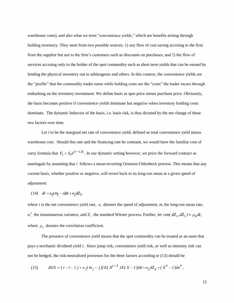
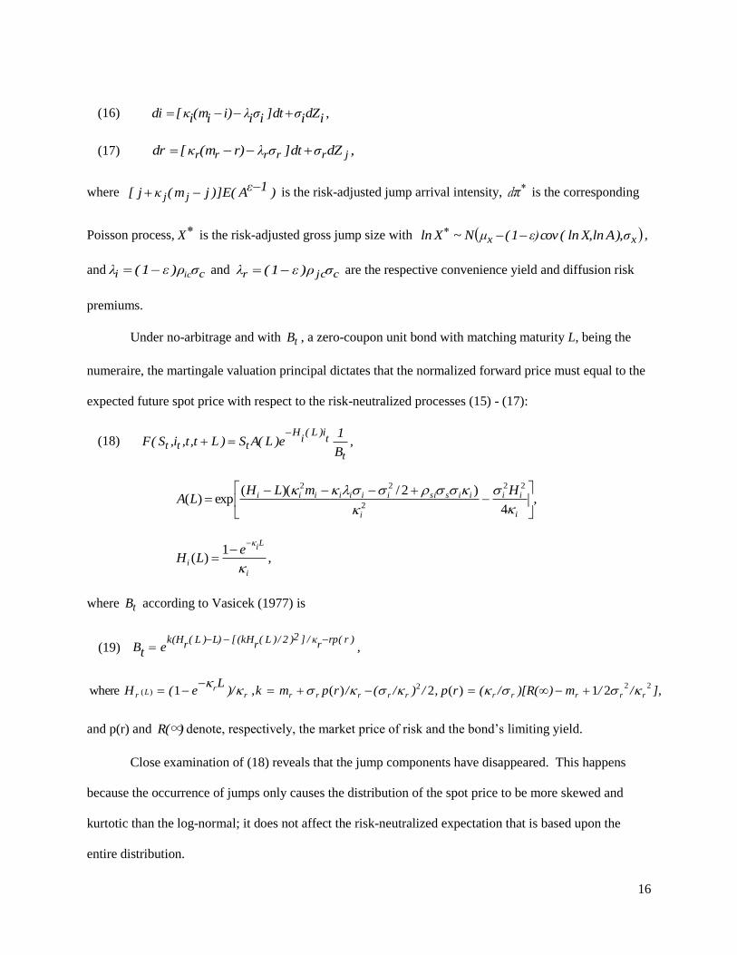
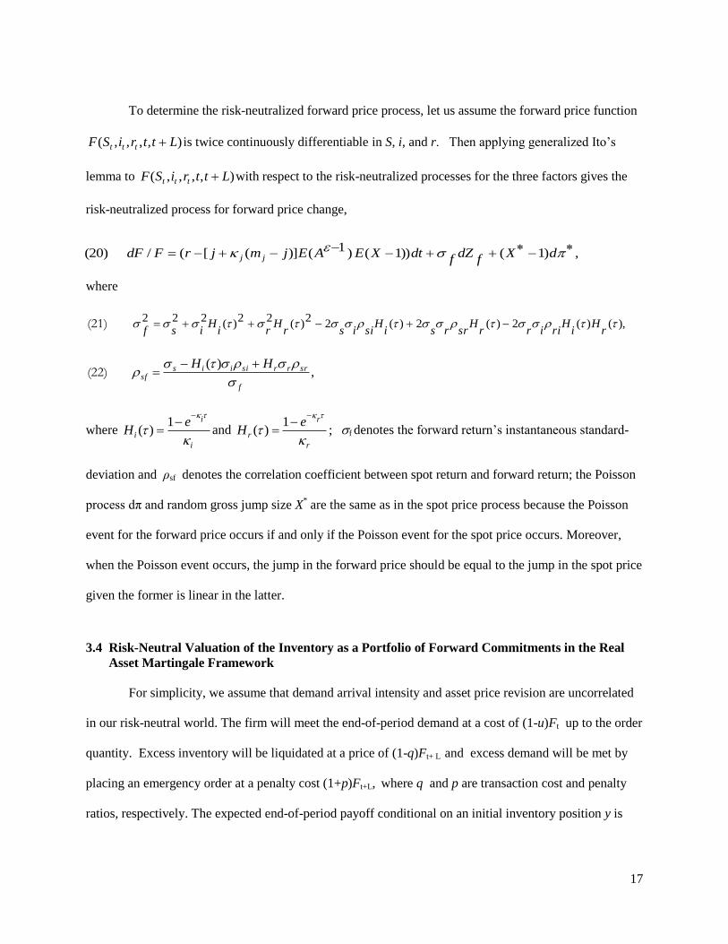
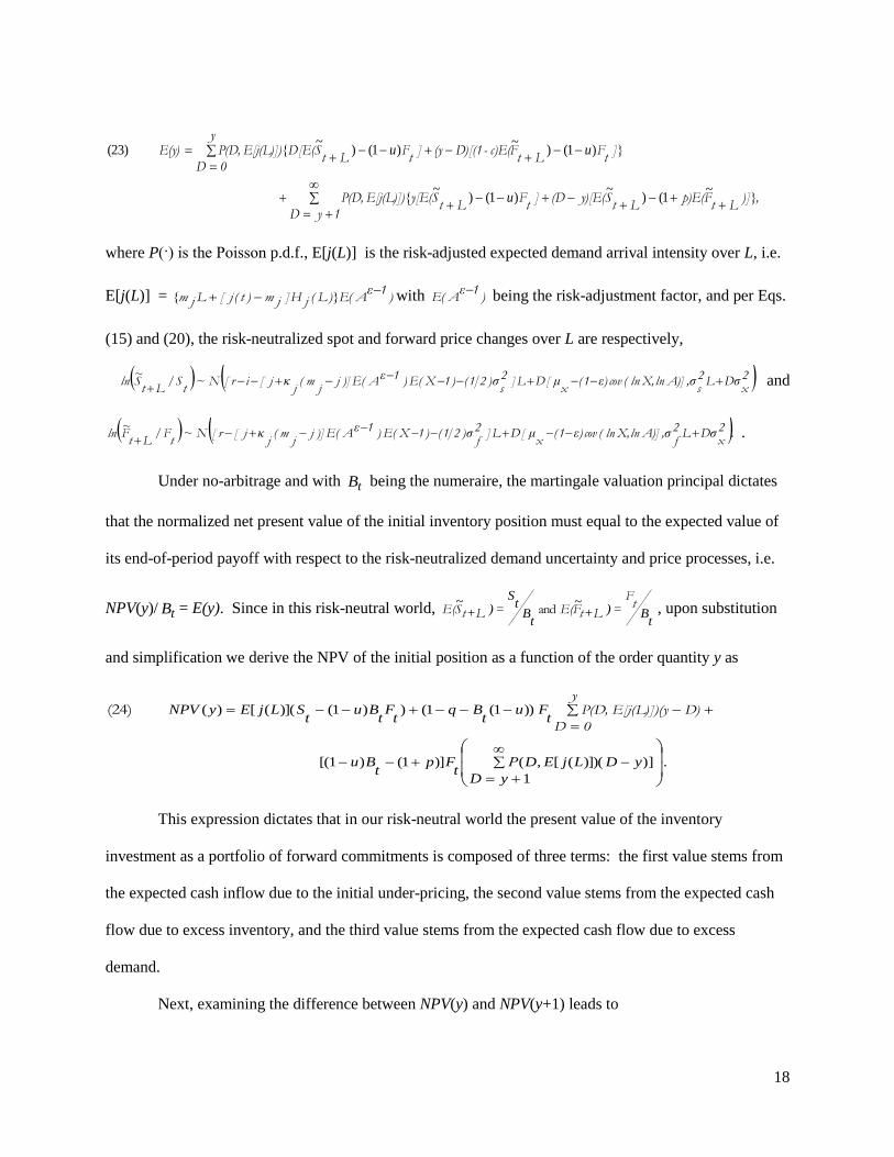
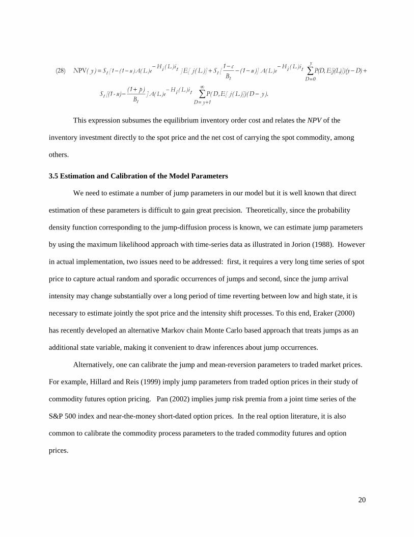
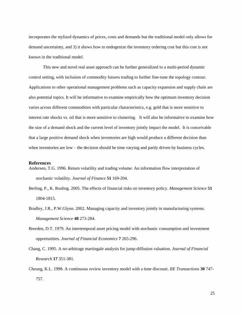
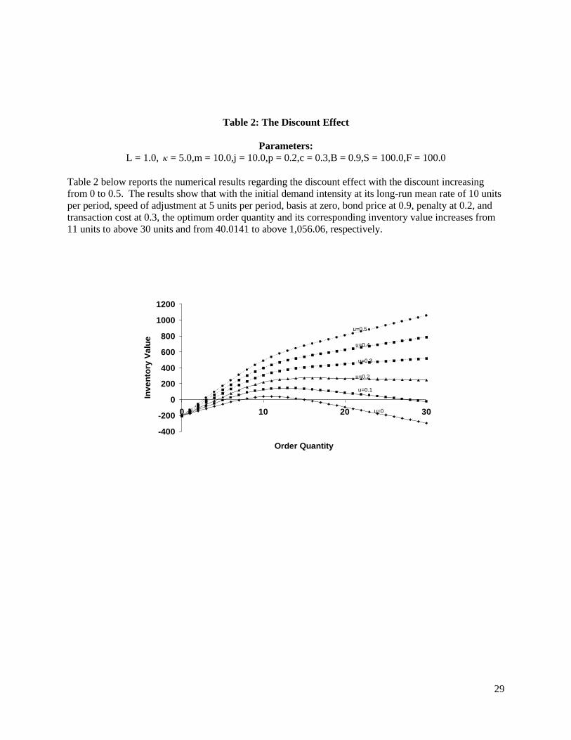
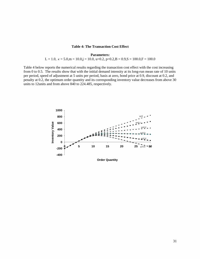
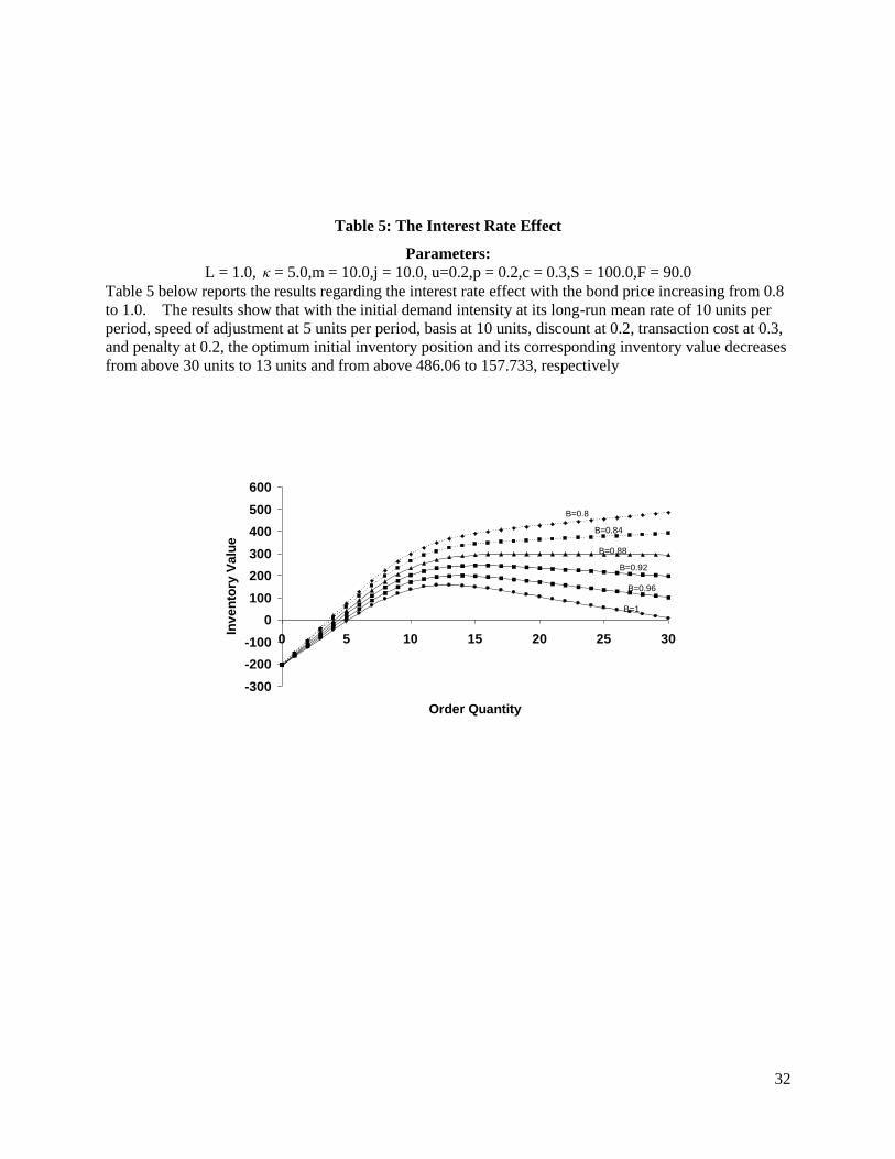
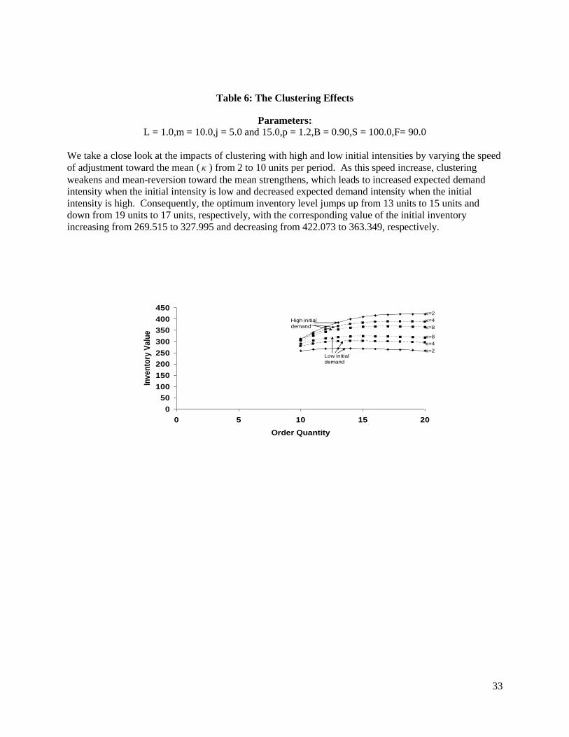
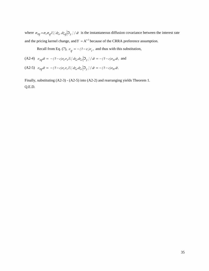


![ASSET Valuation[1]](https://img.pdfslide.us/doc/110x75/577d27af1a28ab4e1ea48bd2/asset-valuation1.jpg)