Progress In Electromagnetics Research C, Vol. 37, 15–28, 2013

A MAGNETO-INDUCTIVE LINK BUDGET FOR WIRE-LESS POWER TRANSFER AND INDUCTIVE COMMU-NICATION SYSTEMS

Johnson I. Agbinya*

Department of Electronic Engineering, La Trobe University, KingsburyDrive, Bundoora, Victoria 3083, Australia

Abstract—This paper presents a propagation model and inductivelink budget based on link equations for chains of inductive loops as thebasis for determining the link budget of inductive communication andwireless power transfer systems. The link between the transmitter andreceiver is modeled in similar format as in radio frequency systems.The transmitter antenna gain, path loss model and receiver antennagain are also modeled for the inductive case. This allows the magneticpath loss to be estimated accurately. Also the induced receiver currentdue to a transmitter voltage can be computed apriori enabling efficientdesign of inductive links and transceivers.

1. INTRODUCTION

A great deal of propagation models and link budget expressions existfor radio wave propagation at different frequencies and in differentterrains. However, when it comes to inductive communication, nopropagation models and link budgets similar to Lee [1], Hata, COST231 and Stanford University Interim (SUI) models [2] exist in currentliterature. This could be mainly due to the limited research oninductive communications to date. However, interest in magneticinduction (MI) systems operating as wireless power transfer andcommunication transceivers has increased greatly within the last fewyears because of their inherent properties. Inductive systems do notinterfere with existing traditional electromagnetic wave radiators inmost bands. To their advantage magnetic induction communicationsystems are also not generally affected by the environment. In factthe only parameter in the MI power equation and link budget that

Received 5 December 2012, Accepted 19 January 2013, Scheduled 24 January 2013* Corresponding author: Johnson Ihyeh Agbinya (j.agbinya@latrobe.edu.au).

16 Agbinya

has to do with the environment is the permeability of the materialsin the link and source (sink) which acts to enhance the receivedsignal. Hence the permeability of the medium can be used toenhance the power transfer in the link. Therefore issues such asfading, multipath propagation, interference and noise which plagueelectromagnetic (EM) systems are not problems in MI communicationsystems. Inductive systems are however very short range technologiesdue to rapid decay with distance of the flux created by the varyingtransmitter current. Applications of inductive methods have becomemore and more widespread including transcutaneous systems [3],near-field voice communications [4], wireless power transfer [5], datatransmission systems [6], underground communications [7, 8], linksand communication channels inside integrated circuits [6]. Many ofthese applications use several coils to either extend the range of theapplication or to deliver power more efficiently. The more coils usedthe more the number of equations that must be solved to determine thetransfer function of the system. One of such applications where manycoils are used is in magneto-inductive waveguides. Magneto-inductivewaveguides have recently emerged as a method of extending the rangeof MI communications systems. The pioneering works of Syms et al. [9–14] and Kalinin et al. [15] have established some of the theories for theMI waveguides. Recently the authors also demonstrated relaying inMI systems [21, 22]. These systems involve arrays of coils arranged asresonant chain networks or in multiple paths to create multipath relaynodes. The solutions to their lumped circuit models normally involvesolving systems of simultaneous equations which are prone to mistakesbecause of the number of variables and equations involved. A systemof N resonating nodes requires (N + 1) simultaneous equations to besolved and becomes very difficult when N is large. The objective ofthis paper is to propose a fast solutio method in other to simplify thisrigour.

The methods of link budgets for traditional radio frequency (RF)communications are well established and understood. A link budgetpresents a summary of how the transmitted power is spent in thecommunication chain between the transmitter and receiver. Systemgains are presented as positive values and losses as negative valuesin decibels. Over the last couple of years attempts have been madetowards developing link budget expressions for inductive systems asgiven in [15–22]. Lack of consistency in the formulations of the linkbudget expressions which limits their use motivates this paper.

Inductive links to date have been developed as chain networksin which one loop induces flux on its neighbor until the data fluxis received by the last loop to which the load is connected. Usually

Progress In Electromagnetics Research C, Vol. 37, 2013 17

the systems have line-of-site of each other and are aligned along thecommon axis of the coils. Such systems may therefore be modeled asresonating magneto-inductive waveguides. Therefore in this paper theanalysis leading to the elegant expression for the inductive link budgethas used this approach as depicted in Figure 1. The rest of the paper isorganized as follows. Section 2 develops expressions for inductive linksusing the magneto-inductive waveguide formulation. Simulations ofthe links are presented in the same section. In Section 3, the magneticlink equation is derived and used to propose a link budget expressionfor low coupling applications. In Section 4, methods for assessing theefficiency of the magnetic link are proposed with conclusions drawn inSection 5.

2. INDUCTIVE LINKS

In its simplest form, a one section peer-to-peer magnetic field couplingsystem is used for wireless power transfer and communication in thetraditional MI system with no options of range extension (Figure 1).This model has been well analyzed and discussed by Agbinya et al. [6].The lumped circuit model of the system is also shown in Figure 1.An N -section waveguide extends this simple formulation by using Nresonating coils or split-ring resonators. Figure 1 shows the multiplecoil array version of the system. We assume each coil is loaded with acapacitor to resonate and the receiver has a load ZL. The currentin each loop n is therefore In. We assume only nearest neighborinteraction in which only currents in node n− 1 and n + 1 affect noden. we also assume that the N nodes are resonating at frequency ω0.Node n has impedance Zn and current In. Node n = 1 is excited withinput voltage and the rest couple magnetic fields from one to the otheruntil the receiver node is reached. The intermediate nodes are passivebut the receiver has load impedance ZL.

2.1. Power Relations in Inductive Links

The purpose of this section is to establish a system equation whichis repeatable and easily usable in a form similar to the propagationequation in basic electromagnetic communications systems. To do this,let us consider a peer-to-peer inductive communication consisting oftwo loops, a transmitter and receiver loops. The governing equationsfor the system (Figure 1) are:

Z1I1 + jωM12I2 = Us (1)

Z2I2 + jωM12I1 = 0 Mij = kij

√LiLj 0 ≤ kij ≤ 1 (2)

18 Agbinya

Us

Z1

ZL

Z2

UM

1Z'

2Z '

Us

R1 R2

L2L1

M

ZL

r1r2

d

α

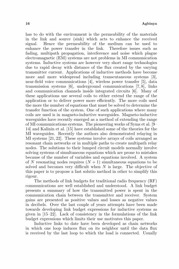
Figure 1. MI communication system.

where the transmitter and receiver loop impedances are Z1 and Z2

with currents flowing through them as I1 and I2 respectively. Themutual inductance and the coupling coefficient between them writtenin general terms are Mij and kij respectively (i = 1, j = 2). Let thetransmitter parameters have index ‘1’ and index ‘2’ be reserved for thereceiver variables. The impedances Z ′2 refer to the influences of thetransmitter on the receiver and of the receiver on the transmitter Z ′1.

The voltage developed across the receiver load due to inductiveaction is given by the expression

VL = I2ZL (3)

where in general for a system consisting of multiple intermediate (orrelay) nodes each loop impedance is

Zn = Rn + jωLn +1

jωCn(4)

The impedance of the receiver when the load impedance is consideredis

Zr = R2 + jωL2 +1

jωC2+ ZL (5)

By solving Equations (1) to (5) simultaneously, the ratio of the loadvoltage to that of the source is given by the expression:

Gv =VL

US=

−jωM12ZL

ω2M212 + Z1Z2

(6)

The gain function Gv relates the input voltage (US) to the voltage VL

developed across the receiver load ZL. It relates the system parametersfor the transmitter and receiver including the link between them. This

Progress In Electromagnetics Research C, Vol. 37, 2013 19

expression may also be written in terms of the current induced in thereceiver coil as:

Gv (ω) =IL

US=

−jωM12

ω2M212 + Z1Z2

(7)

where IL = I2 = VL/ZL = GvUS . The power delivered to the receiverload is the product I2

LZL = I2I∗2ZL.

2.1.1. Approximate Wireless Power Transfer Equation for a Link

Equation (7) is a simple case because it involves solving only threeequations but once the number of loops increase and for N loops(N + 1) equations are required, solving the equations to obtain Gv(ω)becomes a lot more difficult and time consuming. A preferred approachis to develop a link equation which relates multiple loops in termsof the input transmitter voltage to the inductive current flowingthrough the load impedance. Let the quality factors of the transmitterand receiver coils be Q1 = ωL1/R1; Q2= ωL2/R2 and replacing themutual inductance with an equivalent expression containing the qualityfactors, the expression for the inductive system gain at resonancebecomes

IL

US=

−jk12√

Q1Q2√R1R2

(k2

12Q1Q2 + 1) (8)

At low coupling and small quality factors (Q), the inequalitiesk2

12Q1Q2 ¿ 1 or k212 ¿ 1/Q1Q2 hold. Therefore the inductive transfer

function at resonance reduces to.∣∣∣∣IL

US

∣∣∣∣ =k12√

Q1Q2√R1R2

=kij

√QiQj√

RiRj

(9)

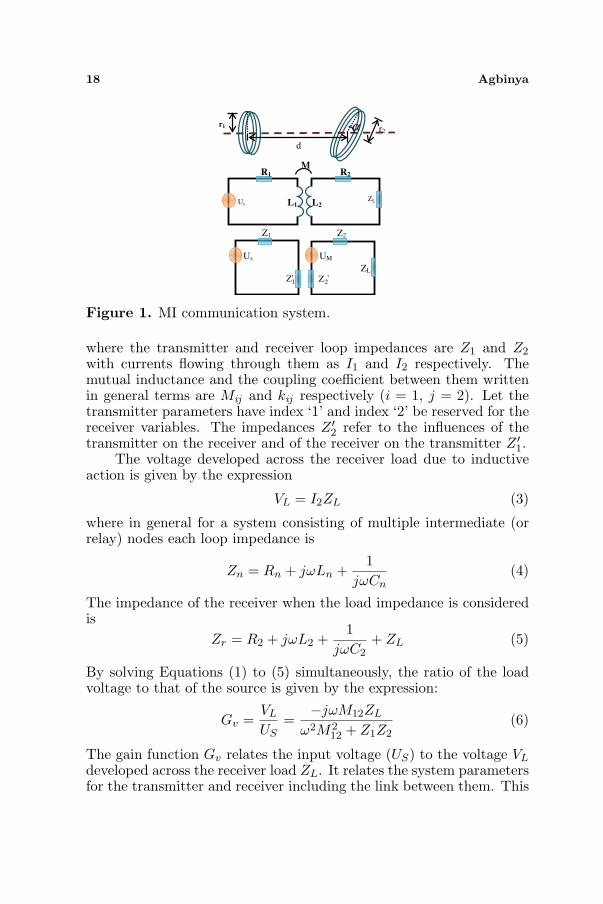
We have simulated Equations (8) and (9) in Matlab. Figures 2(a) and(b) show the simulation for the low coupling approximation when thetwo coils have identical Q = 2 and Q = 10 respectively and k = 0.1.The approximation is very accurate for low k and low Q but starts todeviate for higher Q. Figure 2(c) shows the variation of the transferfunction with Q and plotted as a function of the logarithm of themagnitude of the numerator of Equation (8). Using the horizontalaxis from these figures, it is apparent that the approximation is validat high Q when the numerator is nearly equal to the denominator.Very high Q causes a deviation from the general solution.

2.1.2. Approximate Wireless Power Transfer Link Equations

The use of multiple inductive loops (Figure 4) in a chain networkis more popular than the simple two loops system. Increasing the

20 Agbinya

(a)

(b) (c)

Figure 2. Compared transfer functions with/without approximation(N = 2). (a) Compared transfer function at low Q (red curve iswith approximation; blue curve has no approximation. (b) Comparedtransfer function at high Q, with approximation (read curve); withoutapproximation (blue curve). (c) Variation of transfer function with Q.

number of loops is used to improve the power transfer efficiency andfor extending the communication range. Consider a three node systemwith the following Kirchhoff voltage law (KVL) equations:

Z1I1 + jωM12I2 = Us

Z2I2 + jωM12I1 + jωM23I3 = 0Z3I3 + jωM23I2 = 0VL = I3ZL

(10)

Solving the simultaneous Equation (10) results to the expression:

VL

US=

ω2M12M23ZL

ω2(M2

12Z3 + M223Z1

)+ Z1Z2Z3

(11)

Progress In Electromagnetics Research C, Vol. 37, 2013 21

(a) (b)

Figure 3. Power transfer functions with approximation (N = 3). (a)Power transfer function when Q = 2; Red = approximation; Blue =no approximation. (b) Power transfer function when Q = 10; Red =approximation; Blue = no approximation.

Figure 4. Magnetic waveguide and its circuit model.

At resonance this equation can be simplified and becomes

IL

US=

k12k23Q2√

Q1Q3√R1R3

[1 + k2

12Q1Q2 + k223Q2Q3

] (12)

As in Equation (8), we consider low coupling when k212Q1Q2 +

k223Q2Q3 ¿ 1 or Q2 ¿ 1/

(k2

12Q1 + k223Q3

)and writing kij = ki,j the

22 Agbinya

low coupling transfer function becomes

∣∣∣∣IL

US

∣∣∣∣ =k12k23Q2

√Q1Q3√

R1R3=

√Q1QN

N−1∏i=1

ki,i+1

N−2∏i=1

Qi+1

√R1RN

(13)

To demonstrate the effectiveness of the approximations, simulationswere undertaken using Matlab. Equation (12) the case for noapproximation and Equation (13) with approximation were used. Thered lines in Figure 3 show the case when no approximations were used.The blue curves are results with approximation. The approximationfor k = 0.1 and Q = 2 is held at N = 3 with slight deviations only forhigher Q = 10. High Q values are normally used in wireless powertransfer systems and the higher the Q the more the deviations inthe curves shown in Figure 3. These approximations are thereforemore suited to low Q systems as in inductive communications. Acorrection term (k2

12Q1Q2) should be used in the denominator ofEquation (13) to reduce the deviation at high Q. The correctionchanges the denominator to

√R1R3

(1 + k2

12Q1Q2

).

We extend the system one more time to demonstrate the conceptfurther for N = 4. In this case the system of equations is

Z1I1 + jωM12I2 = Us

Z2I2 + jωM12I1 + jωM23I3 = 0Z3I3 + jωM23I2 + jωM34I4 = 0Z4I4 + jωM34I3 = 0VL = I4ZL

(14)

This has the solutionVL

US=

jω3M12M23M34ZL

Z1Z2Z3Z4 + ω4M212M

234 + ω2

(M2

12Z3Z4 + M223Z1Z4

+M234Z1Z2

) (15)

At resonance it reduces to∣∣∣∣IL

US

∣∣∣∣ =Q2Q3k12k23k34

√Q1Q4

√R1R4

[1 +

(k2

12Q1Q+k223Q2Q3 + k2

34Q3Q4

)+k2

12k234Q1Q2Q3Q4

] (16)

The low coupling approximation when N = 4 with t(k212Q1Q2 +

k223Q2Q3 +k2

34Q3Q4) + k212k

234Q1Q2Q3Q4 ¿ 1 is

∣∣∣∣IL

US

∣∣∣∣ =k12k23k34Q2Q3

√Q1Q4√

R1R4=

√Q1Q4

3∏i=1

ki,i+1

2∏i=1

Qi+1

√R1R4

(17)

Progress In Electromagnetics Research C, Vol. 37, 2013 23

Normally even when the loops are arranged equidistant from eachother, the strongest coupling is between the first and second loopwith coefficient k12 and the rest of the coefficients become smaller andsmaller towards the receiver.

To accommodate for high coupling situations as in wireless powertransfer, correction terms may also be progressively added to thedenominator of Equation (17).

3. INDUCTIVE LINK EQUATION

The performance of an inductive system is conditioned upon reducinglosses in the transmitter, the receiver and the channel. Both thereceiver and transmitter suffer from resistive losses. The previoussection has provided the basis for assessing the performance of theinductive link. Losses in the transmitter and receiver will be discussedat the end of this section. From Equations (9), (13) and (17) ageneral link equation for N loops in a chain can be derived using thelow coupling approximation and nearest neighbor interaction. UsingEquations (9), (13) and (17) we can show that the link equation andhence the link efficiency ηTR is given by the following expression

ηTR =∣∣∣∣IL

US

∣∣∣∣ =

√Q1QN

N−1∏i=1

ki,i+1

N−2∏i=1

Qi+1

√R1RN

(18)

This is a general expression which holds for all N , provided theapproximations are made in the denominators for the solutions tothe simultaneous KVL equations. Equation (18) represents a generalsimplification of the link equation when multiple loops are involved.To use the equation, it is required that the number of loops N beselected including the electrical dimensions of each loop. The electricaldimensions include the radius ri of each loop, number of turns N , theresistance of each loop Ri, the distance between the loops l whichare then used to compute the quality factors of the loops. Thenselect the excitation voltage US and the load impedance. The loadcould be a sensor or a device being driven by the array of inductiveloops. Therefore the link budget equation for the induced load voltageVL = ILZL is proportional to the square of the voltage across the loadimpedance and is given in decibels for N loops as:

VL (dB) = 20 log10 US + 10 log10 (Q1QN ) + 20N−1∑

i=1

log10 (ki,i+1)

24 Agbinya

+20N−2∑

i=1

log10 (Qi+1)− 10 log10 (R1RN ) (19a)

Generally ki,i+1 ¿ 1. Therefore the third term in Equation (19a) isnegative and the equation is written in decibels as

VL (dB) = US (dB) + Q1N (dB)− ki,i+1 (dB)+Qi+1 (dB)−R1N (dB) (19b)

We have used a minus sign following the tradition in RF systemsfor using negative sign for the path loss model. This is because theindividual coupling coefficients are less that one. Note that the indexvariations for the coupling coefficients ki,i+1, 1 ≤ i ≤ N − 1 and forthe quality factors Q, 1 ≤ i ≤ N − 2.

What do Equations (19a) and (19b) represent in terms of wirelesspower transfer and communication using inductive nodes? By definingQ as the gain of a node, the general equation has the followinginterpretation as in traditional RF systems. The product

√Q1QN

is the gain of the transmitter and receiver stages. This is similar to theproduct of the transmitter and receiver antenna gains in RF systems.

The quantityN−2∏i=1

Qi+1 is the product of the gains of the intermediate

or relay stages. This is also similar to the product of the gains of the

intermediate stages in a transponder system. The termN−1∏i=1

ki,i+1 is

the path loss of the general magnetic channel. Thus we model theoverall system of N resonating inductive loops as in Figure 5.

The resistors R1 and RN are the inherent Ohmic losses ofthe transmitter and receiver stages. The inductive system has a

channel with path loss (gain) equal to Gc =N−1∏i=1

ki,i+1

N−2∏i=1

Qi+1.

If as in transcutaneous systems applications or in embeddedbiomedical systems when biological tissues are part and parcel of thechannel between the transmitter and receiver, and if the biologicalchannel has impedance Zb, the channel gain is modified to Gc =

Zb

N−1∏i=1

ki,i+1

N−2∏i=1

Qi+1 and the channel becomes a function of frequency

and leads to further coupling losses between the transmitter andreceiver. Most importantly, Equations (19a) and (19b) may be usedto estimate the various system parameters during the design processto enable a required inductive current in the receiver load of the Nthloop.

Consider as an example an inductive waveguide link system

Progress In Electromagnetics Research C, Vol. 37, 2013 25

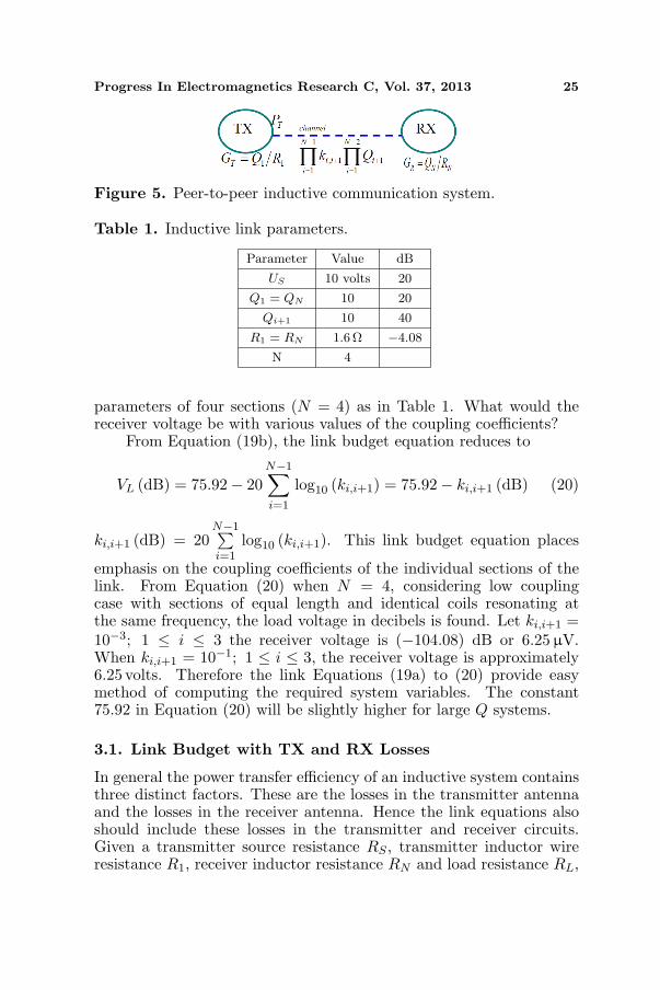
Figure 5. Peer-to-peer inductive communication system.

Table 1. Inductive link parameters.

Parameter Value dB

US 10 volts 20

Q1 = QN 10 20

Qi+1 10 40

R1 = RN 1.6Ω −4.08

N 4

parameters of four sections (N = 4) as in Table 1. What would thereceiver voltage be with various values of the coupling coefficients?

From Equation (19b), the link budget equation reduces to

VL (dB) = 75.92− 20N−1∑

i=1

log10 (ki,i+1) = 75.92− ki,i+1 (dB) (20)

ki,i+1 (dB) = 20N−1∑i=1

log10 (ki,i+1). This link budget equation places

emphasis on the coupling coefficients of the individual sections of thelink. From Equation (20) when N = 4, considering low couplingcase with sections of equal length and identical coils resonating atthe same frequency, the load voltage in decibels is found. Let ki,i+1 =10−3; 1 ≤ i ≤ 3 the receiver voltage is (−104.08) dB or 6.25 µV.When ki,i+1 = 10−1; 1 ≤ i ≤ 3, the receiver voltage is approximately6.25 volts. Therefore the link Equations (19a) to (20) provide easymethod of computing the required system variables. The constant75.92 in Equation (20) will be slightly higher for large Q systems.

3.1. Link Budget with TX and RX Losses

In general the power transfer efficiency of an inductive system containsthree distinct factors. These are the losses in the transmitter antennaand the losses in the receiver antenna. Hence the link equations alsoshould include these losses in the transmitter and receiver circuits.Given a transmitter source resistance RS , transmitter inductor wireresistance R1, receiver inductor resistance RN and load resistance RL,

26 Agbinya

the transmitter efficiency is ηT and the receiver efficiency is ηR. Hencethe the overall system link efficiency is,

η = ηT ηTRηR;

ηT = RS

RS+R1

ηR = RLRL+RN

(21)

With this correction, the link Equations (19a) to (20) need to bemodified to include these terms. Since ηT < 1 and ηR < 1, the overallsystem link budget expression is obtained by modifying Equation (19b)to be:

VL (dB) = −ηT + US (dB) + Q1N (dB)− ki,i+1 (dB) + Qi+1 (dB)−R1N (dB)− ηR (22)

The two new terms are marginal corrections which should beimplemented to account for the resistive losses in the transmitter andreceiver coils.

3.2. Correction TermsAs in RF propagation models and link budgets, progressive correctionterms may be added to the denominator of the transfer functionequation and hence to the link budget equation in decibels. Thesecorrections apply for high Q when only the first loop is excitedwith input voltage at frequency ω. For example, when N = 2 thecorrection term is k2

12Q1Q2. When N = 3, there are two termsk2

12Q1Q2+k223Q2Q3 that could be used for corrections and are functions

of k212 and k2

23. If the nodes are distributed evenly in a chain networkso that the distance between nodes is constant x, then k2

23 < k212 and

to improve upon the approximation the term k212Q1Q2 may be added

as correction. For N > 3, progressive corrections may be made forhigher k(Q) based on adding terms in k2

ij where i, and j are integers.

4. CONCLUSIONS

We have developed an accurate expression for link budgets of inductivesystems. The algorithm presented enables accurate estimation ofinductive loop system gains. They could be used for designingand assessing the performances of embedded biomedical data andwireless power transfer, personal area networks and communicationsunderground. The link budget applies for all N and eliminates theneed to solve a large system of equations, provided the couplingcoefficients and the quality factors of the loops are computed andknown. Progressive corrections to account for larger k and Q canbe made for large k and Q applications.

Progress In Electromagnetics Research C, Vol. 37, 2013 27

REFERENCES

1. Lee, D. J. Y. and W. C. Y. Lee, “Enhanced Lee model fromrough terrain data sampling aspect,” Proc. IEEE 72nd VehicularTechnology Conference Fall (VTC 2010-Fall), 1–5, 2010.

2. Castro, B. S. L., I. R. Gomes, F. C. J. Ribeiro, and G. P. S. Cav-alcante, “COST231-Hata and SUI models performance using aLMS tuning algorithm on 5.8 GHz in Amazon region cities,” Proc.Fourth European Conference on Antennas and Propagation (Eu-CAP), 1–3, 2010.

3. Chen, Q., S. C. Wong, C. K. Tse, and X. Ruan, “Analysis, design,and control of a transcutaneous power regulator for artificialhearts,” IEEE Transactions on Biomedical Circuits & Systems,Vol. 3, No. 1, 23–31, 2009.

4. Agbinya, J. I., “Framework for wide area networking of inductiveInternet of things,” Electronics Letters, Vol. 47, No. 21, 1199-1201,Oct. 13, 2011.

5. Kurs, A., A. Karalis, R. Moffatt, J. D. Joannopoulos, P. Fisher,and M. Soljacic, “Wireless power transfer via strongly coupledmagnetic resonances,” Sci., Vol. 317, 83–86, Jul. 2007.

6. Agbinya, J. I., N. Selvaraj, A. Ollett, S. Ibos, Y. Ooi-Sanchez,M. Brennan, and Z. Chaczko, “Size and characteristics of the‘cone of silence’ in near field magnetic induction communications,”Journal of Battlefield Technology, Mar. 2010.

7. Sun, Z. and I. F. Akyildiz, “Underground wireless communicationusing magnetic induction,” Proc. IEEE ICC 2009, Dresden,Germany, Jun. 2009.

8. Akyildiz, I. F., Z. Sun, and M. C. Vura, “Signal propagationtechniques for wireless underground communication networks,”Physical Communication, Vol. 2, 167–183, 2009 (in Elsevier).

9. Syms, R. R. A., E. Shamonina, and L. Solymar, “Magneto-inductive waveguide devices,” Proceedings of IEE Microwaves,Antenna and Propagation, Vol. 153, No. 2, 111–121, 2006.

10. Syms, R. R. A. and L. Solymar, “Bends in Magneto-inductivewaveguides,” Metamaterials, 2010.

11. Syms, R. R. A., L. Solymar, I. R. Young, and T. Floume, “Thin-film magneto-inductive cables,” Journal of Physics D, Vol. 43,2010.

12. Syms, R. R. A., L. Solymar, and I. R. Young, “Three-frequencyparametric amplification in magneto-inductive ring resonators,”Metamaterials, Vol. 2, 122–134, 2008.

13. Syms, R. R. A., I. R. Young, and L. Solymar, “Low-loss magneto-

28 Agbinya

inductive waveguides,” Journal of Physics D: Applied Physics,Vol. 39, 3945–3951, 2006.

14. Syms, R. R. A., O. Sydoruk, E. Shamonina, and L. Solymar,“Higher order interactions in magneto-inductive waveguides,”Metamaterials, Vol. 1, 44–51, 2007.

15. Kalinin, V. A., K. H. Ringhofer, and L. Solymar, “Magneto-inductive waves in one, two and three dimensions,” Journal ofApplied Physics, Vol. 92, No. 10, 6252–6261, 2002.

16. Agbinya, J. I. and M. Masihpour, “Near field magnetic inductioncommunication link budget: Agbinya-Masihpour model,” Proc. ofIB2Com, 1–6, Malaga, Spain, Dec. 15–18, 2010.

17. Fatiha, E. H., G. Marjorie, P. Stephane, and P. Odile, “Magneticin-body and on-body antennas operating at 40 MHz and near fieldmagnetic induction link budget,” Proc. EuCAP, 1–5, 2012.

18. Azad, U., H. C. John, and Y. E. Wang, “Link budget andcapacity performance of inductively coupled resonant loops,”IEEE Transactions on Antennas and Propagation, Vol. 60, No. 5,2453–2461, May 2012.

19. Ramos, G. V. and J.-S. Yuan, “FEM simulation to characterizewireless electric power transfer elements,” 2012 Proceedings ofIEEE Southeastcon, 1–4, Mar. 15–18, 2012.

20. Fatiha, E. H., G. Marjorie, S. Protat, and O. Picon, “Link budgetof magnetic antennas for ingestible capsule at 40 MHz,” ProgressIn Electromagnetics Research, Vol. 134, 111–131, 2013.

21. Masihpour, M. and J. I. Agbinya, “Cooperative relay in nearfield magnetic induction: A new technology for embedded medicalcommunication systems,” Proc. of IB2Com, Malaga, Spain,Dec. 15–18, 2010.

22. Agbinya, J. I. and M. Masihpour, “Magnetic induction channelmodels and link budgets: A comparison between two Agbinya-Masihpour models,” Proc. the Third International Conferenceon Communications and Electronics (ICCE 2010), 400–405, NhaTrang, Vietnam, Aug. 11–13, 2010.