Embed Size (px)
Citation preview

A Macro-Finance Model with Sentiment∗
Job Market Paper
Latest Version: Available Here
Peter Maxted
Harvard University
November 13, 2020
Abstract
This paper integrates diagnostic expectations into a general equilibrium macroe-
conomic model with a financial intermediary sector. Diagnostic expectations
are a forward-looking model of extrapolative expectations that overreact to
recent news. Frictions in financial intermediation produce nonlinear spikes in
risk premia and slumps in investment during periods of financial distress. The
interaction of sentiment with financial frictions generates a short-run amplifi-
cation effect followed by a long-run reversal effect, termed the feedback from
behavioral frictions to financial frictions. The model features sentiment-driven
financial crises characterized by low pre-crisis risk premia and neglected risk.
The conflicting short-run and long-run effect of sentiment produces boom-bust
investment cycles. The model also identifies a stabilizing role for diagnostic
expectations. Under the baseline calibration, financial crises are less likely to
occur when expectations are diagnostic than when they are rational.
∗Email: [email protected]. I would like to thank Francesca Bastianello, Pedro Bordalo,John Campbell, Daniele d’Arienzo, Emmanuel Farhi, Paul Fontanier, Xavier Gabaix, Nicola Gen-naioli, Thomas Graeber, Samuel Hanson, Zhiguo He (discussant), Arvind Krishnamurthy, SpencerYongwook Kwon, David Laibson, Lu Liu, Matteo Maggiori, Andrei Shleifer, Jakob Ahm Sørensen,Jeremy Stein, Ludwig Straub, Yeji Sung (discussant), Stephen Terry, Emil Verner, and participantsat the NBER Behavioral Finance Conference for helpful discussion and comments.
1
1 Introduction
Models of financial frictions successfully replicate crisis-driven spikes in risk premia
and the transmission of financial sector vulnerabilities into aggregate downturns.
However, the rational expectations version of these models struggles to match the
empirical pattern of low risk premia in the lead-up to crises. Baron and Xiong (2017)
find that bank equity is overvalued prior to financial crises due to overoptimistic be-
liefs. Krishnamurthy and Muir (2020) show that credit spreads are regularly “too
low” before financial crises, and that frothy financial markets predict future crises.
This conclusion is strengthened in Greenwood et al. (2020a), who document that the
combination of rapid credit and asset price growth is highly predictive of future fi-
nancial crises. All three papers conclude from this pre-crisis evidence that systemic
crash risk is neglected during the buildup to crises.
These findings are not unique to crises. Patterns of excessive optimism preceding
economic downturns appear consistently (Greenwood and Hanson, 2013, Lopez-Salido
et al., 2017). This is supported by direct expectations data from professional fore-
casters, which displays cyclical overreaction to recent macro-financial trends (Mian
et al., 2017, Bordalo et al., 2018b, Bordalo et al., 2020).
In this paper I propose a macro-finance model that is consistent with this evidence
of non-rational expectations. To do so, I incorporate diagnostic expectations into
a macroeconomic model with a financial intermediary sector. Frictions in financial
intermediation allow the model to capture the nonlinear behavior of risk premia during
crises and the asymmetric effect of financial fragility on macroeconomic dynamics.
However, under rational expectations the model relies on a long sequence of negative
shocks to set crises in motion. By introducing behavioral frictions to this model
of financial frictions, this paper is able to investigate the sentiment-driven triggers
of financial fragility. The contribution of this paper is its characterization of the
endogenous financial market and business cycle dynamics that are generated by the
interaction of sentiment and financial frictions.
2
The economic model is based on He and Krishnamurthy (2019). This is a continuous-
time RBC model augmented with a financial intermediary sector. Intermediaries are
subject to an occasionally binding equity issuance constraint. In non-distress periods
the model behaves similarly to a frictionless RBC model. A sequence of poor returns
moves intermediaries closer to their constraint and leads to financial distress. In dis-
tress periods the nonlinearities arising from financial frictions become quantitatively
important. Financial crises are triggered in the tail state where the constraint binds,
causing risk premia to spike and asset prices to plummet.
I depart from rational expectations by introducing behavioral frictions to this
model of financial intermediary frictions. This paper develops a method for extending
rational models with a continuous-time variant of diagnostic expectations. Diagnos-
tic expectations are a forward-looking model of extrapolative expectations in which
agents overweight future states that are representative of recent news (Bordalo et al.,
2018a). When recent shocks have tended to be positive, agents are overoptimistic
about future economic growth. The reverse holds for negative shocks. Diagnostic
expectations do not add an independent source of shocks to the model. Instead,
diagnostic expectations alter the way that shocks drive the economy in equilibrium.
The interaction of diagnostic expectations with frictions in financial intermedia-
tion produces conflicting short-run and long-run dynamics. A sequence of positive
shocks alleviates financial frictions. This increases asset prices and investment. In the
short run, diagnostic expectations amplify this effect. Positive shocks induce overopti-
mism about fundamentals, which further elevates asset prices and investment. In the
long run, this paper identifies a novel feedback from behavioral frictions to financial
frictions that reverses the short-run effect. Elevated sentiment induces a progressive
erosion of intermediary risk-bearing capacity as expectations are disappointed.
I present three results arising from the interaction of behavioral and financial
frictions. First, the model produces sentiment-driven financial crises. Overoptimism
dislocates asset prices from fundamentals. The inflation of asset prices initiates a
3
feedback from behavioral frictions to financial frictions that impairs the risk-bearing
capacity of intermediaries and heightens financial fragility in the background of seem-
ingly low-risk environments. Consistent with the empirical findings outlined above,
sentiment-driven crises feature low pre-crisis risk premia and neglected crash risk.
Second, the interaction of sentiment with financial frictions produces boom-bust
fluctuations in investment and output growth. These cyclical business cycle dynamics
are driven by the conflicting short-run and long-run effect of diagnostic expectations.
Sentiment-driven amplification in the short run begets its own financial-frictions-
driven reversal in the long run.
Third, though diagnostic expectations amplify business cycles, diagnostic expec-
tations can simultaneously stabilize financial cycles. Under the baseline calibration,
financial crises are less likely to occur when expectations are diagnostic than when
they are rational. This possibility sits in direct opposition to the typical narrative
that extrapolative expectations create financial fragility (e.g., the Financial Instabil-
ity Hypothesis of Minsky (1977)). Since sentiment tracks recent economic shocks,
sentiment is typically depressed during periods of financial distress. The long-run
feedback effect of depressed sentiment increases intermediary returns relative to ex-
pectations. This repairs intermediary balance sheets and reduces the potential for
financial distress to erupt into a full-blown crisis.
By interacting sentiment and financial frictions, this paper identifies a long-run
feedback from behavioral frictions to financial frictions that is a key driver of equilib-
rium dynamics. I explore three predictions to evaluate whether this feedback effect
improves the model’s empirical fit. First, the feedback effect produces long-run re-
versals. I examine the persistence of financial distress, the price-dividend ratio, and
the investment-output ratio. In all three cases, the shorter persistence produced by
diagnostic expectations improves the model’s fit. Second, the feedback effect implies
that elevated sentiment generates financial market overheating that can trigger the
emergence of financial fragility. Once this fragility has been triggered, however, it
4
can persist even after sentiment has subsided. I use this prediction to identify a new
fact about financial markets in the buildup to crises: the first eruption of a financial
crisis is often preceded by frothy financial markets, but this is rarely the case for
residual “double-dip” crises. Third, I evaluate the prediction of sentiment-driven fi-
nancial crises by applying the model to the 2007-2008 Financial Crisis. This exercise
suggests that overoptimism in the mid-2000s was critical for exacerbating financial
market vulnerability prior to the failure of Lehman Brothers.
The analysis in this paper relies on two methodological contributions. First, this
paper develops a method for applying diagnostic expectations to an endogenous eco-
nomic growth process. I use this method to generalize the He and Krishnamurthy
(2019) model with non-rational expectations. This allows for the study of beliefs
without compromising the equilibrium dynamics on which sentiment can interact.
Indeed, a key takeaway from this paper is that both behavioral and financial frictions
are necessary for understanding the evolution of the economy around financial crises.
Second, this paper highlights the benefits of using global solution methods for
characterizing the full equilibrium impact of beliefs on economic dynamics. The
analysis of sentiment-driven expansions and slumps fundamentally requires evaluat-
ing the cyclical effects of expectations away from the steady state. Global solution
methods characterize the complete nonlinear dynamical system.
Related Literature. This paper builds on a large financial frictions literature.
Seminal work includes Kiyotaki and Moore (1997) and Bernanke et al. (1999). Recent
research often uses continuous-time methods to analyze global dynamics in models
with nonlinearities. Examples include Adrian and Boyarchenko (2012), He and Krish-
namurthy (2013, 2019), Brunnermeier and Sannikov (2014), Di Tella (2017), Maggiori
(2017), and Moreira and Savov (2017).
There is a growing theoretical literature on credit cycles and the behavioral triggers
of crises. Bordalo et al. (2018a) develop the original model of diagnostic expectations.
Bordalo et al. (2019a) quantify the business cycle implications of diagnostic expec-
5
tations in a partial equilibrium heterogeneous-firm model. Gennaioli and Shleifer
(2018) summarize the research on diagnostic expectations and present a belief-driven
narrative of the 2007-2008 Financial Crisis. The authors identify understanding the
interaction between beliefs and financial frictions as a key “open problem,” which this
paper aims to address.
The contribution of this paper is the analysis of diagnostic expectations jointly
with frictions in financial intermediation. This allows the model to characterize how
sentiment shapes disruptions in financial intermediation, and how this propagates to
the real economy. In more recent work, Krishnamurthy and Li (2020) extend the
financial crisis model of Li (2020) with non-rational expectations of bank-run shocks
in order to quantitatively dissect the mechanisms driving “crisis cycles.” Greenwood
et al. (2019), Gertler et al. (2020), and Wachter and Kahana (2020) also study the
effect of beliefs on booms and busts in financial markets. While this paper contributes
to a growing literature studying the behavioral drivers of financial crises, rational ex-
planations have also been forwarded to account for certain pre-crisis patterns (Gomes
et al., 2018, Farboodi and Kondor, 2020). Barberis (2018) surveys the research on
extrapolative expectations and their application in macro-finance.
This paper also contributes to a budding literature on general equilibrium macroe-
conomic theory augmented with behavioral features. A small set of recent exam-
ples includes Fuster et al. (2012), Woodford (2013), Hirshleifer et al. (2015), Gabaix
(2016), Adam and Merkel (2019), Caballero and Simsek (2020), and Farhi and Wern-
ing (2020).
2 Macro-Finance Model
This paper embeds diagnostic expectations into the macro-finance model of He and
Krishnamurthy (2019, henceforth HK). The HK model is one of the first quantitative
papers in the continuous-time macro-finance literature, and it successfully replicates
the downside macroeconomic risks precipitated by disruptions in financial intermedi-
6
ation. However, because the HK model features rational expectations, risk premia in
this model are always high when financial crises are likely, whereas in the data they
are often low (e.g., Baron and Xiong, 2017, Krishnamurthy and Muir, 2020).
I extend HK in two ways. Most importantly, I generalize the model to allow for
diagnostic expectations. I also introduce a simple labor income margin to improve
the model’s quantitative fit. I adopt HK’s notation when possible.
2.1 Model Setup
Time is continuous, with t denoting the current period. The economy has two sectors:
households and financial intermediaries. The economy has two types of assets in
positive supply: productive capital Kt and housing H.1 The housing supply is fixed
and normalized to H ≡ 1. The price of capital is denoted qt, and the price of housing
is denoted Pt. Asset prices are endogenous and will be determined in equilibrium.
Only intermediaries can directly hold Kt and H.2 Intermediaries fund these pur-
chases by issuing debt and equity to households. Each intermediary faces an “equity
capital constraint” that restricts its ability to raise equity funding. This is the key
financial friction. When binding, intermediaries must replace their equity funding
with additional debt funding.
Output flow Yt is produced according to an “AK” production technology
Yt = AKt. (1)
Parameter A determines the productivity of capital. Capital evolves endogenously
according to:
dKt
Kt
= (it − δ)dt+ σdZt. (2)
1He and Krishnamurthy (2019) use two assets to improve the model’s quantitative predictions.Appendix B.3 provides further discussion.
2The model can be extended to allow households to directly hold a share of Kt and H, but Heand Krishnamurthy (2019) conclude that the quantitative impact is negligible.
7
it is the endogenous rate of capital installation at time t, δ is the exogenous depre-
ciation rate, and {Zt} is a standard Brownian motion. The term σdZt is a capital
quality shock. Capital quality shocks are the only source of uncertainty in the model.
Investment in capital is subject to quadratic adjustment costs. For a gross capital
installation of itKt, the cost is given by Φ(it, Kt) = itKt + ξ2(it − δ)2Kt.
2.2 Diagnostic Expectations
Overview. All agents have diagnostic expectations about the log capital stock.3
Capital is the fundamental in this economy — capital alone determines output (Yt =
AKt), and capital quality shocks are the only source of uncertainty.
Diagnostic expectations are based on Kahneman and Tversky’s representativeness
heuristic, defined as follows: “an attribute is representative of a class if it is very
diagnostic; that is, the relative frequency of this attribute is much higher in that class
than in the relevant reference class.” (Tversky and Kahneman, 1983, p. 296) In the
context of expectations, the reference class reflects the absence of new information.
Representative future states are those that become more likely to occur in light of
incoming data.
This paper features two innovations on the original diagnostic expectations model
of Bordalo et al. (2018a). First, diagnostic expectations are cast in continuous time.
Second, the methodology developed here allows diagnostic expectations to be applied
to the endogenous capital process.4 This will imply not only that recent economic
performance affects expectations (a standard feature of extrapolative expectations),
but also that expectations feed back into the dynamical system to alter the future
evolution of the capital process on which expectations are formed.
This section presents the reduced-form specification of diagnostic expectations as
applied to the macroeconomic model. Appendix A.1 provides a microfoundation.
This paper’s specification is designed portably so that diagnostic expectations can
3Log capital evolves according to dkt = (it − δ − σ2
2 )dt+ σdZt.4The Bordalo et al. (2018a) model only applies to exogenous AR(N) processes.
8
be added to rational models using a single additional state variable. Even though
I introduce an additional state variable to the HK model, I do not introduce any
additional shocks. Capital quality shocks remain the sole driving shock in the model.
Expectations of Capital. The psychology of diagnostic expectations is as follows.
Agents have in the back of their mind all necessary information to form correct
expectations. However, limited and selective memory means that representative states
come to mind more easily. Representative states are those that are diagnostic of
incoming data, which in this model corresponds to recent capital quality shocks.
This is formalized in the following measure of “recent information” at time t:
It ≡∫ t
0
e−κ(t−s)σdZs. (3)
It is a weighted integral of past shocks to capital, where the weight decays at rate κ
as shocks occur further in the past.5 It > 0 when recent shocks have tended to be
positive, and It < 0 when recent shocks have tended to be negative. It drifts back to
0 at rate κ in the absence of new shocks.
Throughout, I will use hat notation to denote the beliefs of diagnostic agents.
The current period is t, and let τ ≥ 0 denote a prediction horizon. Diagnostic agents
believe that capital in period t+ τ evolves according to:
dKt+τ
Kt+τ
= (it+τ − δ + θIte−κτ )dt+ σdZt+τ . (4)
Parameter θ governs the extent to which agents judge by representativeness. θ = 0
recovers rationality. When θ > 0, expectations of capital growth are biased toward
states that are diagnostic of recent information. For this reason, information param-
eter It will be referred to as “sentiment” henceforth.
5It is an Ornstein-Uhlenbeck process. In discrete time, any individual shock can itself representnew information. In continuous time, I integrate over the past sequence of shocks because eachindividual shock σdZs has only an infinitesimal effect on the capital stock. My specification issimilar to the definition of sentiment in Barberis et al. (2015).
9
Consider equation (4) when τ = 0: dKt
Kt= (it − δ + θIt)dt + σdZt. Diagnostic
expectations bias the perceived growth rate of capital by θIt. At more distant horizons
(τ > 0), this bias dissipates at rate κ. Information that is diagnostic of economic
conditions at time t slowly dims as the agent forms expectations about the economy’s
evolution in the more distant future.
Equation (4) should be interpreted as an “as if” process. Diagnostic agents do
not consciously calculate the evolution of capital in a biased way. Agents have the
true model in their memory database, but are exceedingly drawn to representative
states. It is an unconscious internal parameter that characterizes the state of repre-
sentativeness at time t.
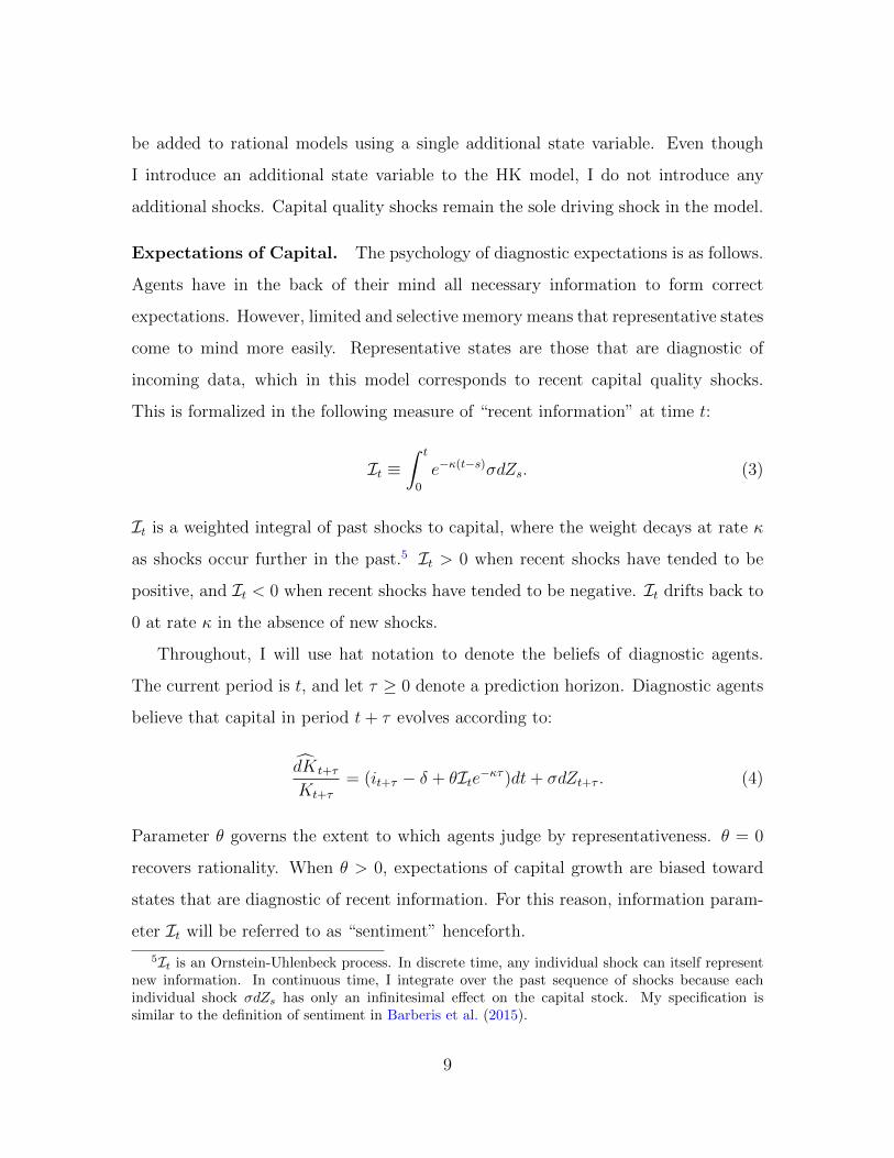
Figure 1 provides an illustrative example of diagnostic expectations applied to an
arithmetic Brownian motion (ABM).6 The blue line plots the realized sample path
of the ABM up to time t. The dashed black line plots the rational prediction of the
ABM’s future path. The solid red line plots the diagnostic prediction. Because recent
shocks have tended to be positive, diagnostic expectations are biased upward.
Figure 1: Diagnostic expectations of arithmetic Brownian motion. The blueline plots the sample path of an arithmetic Brownian motion (ABM). The solid redline plots diagnostic expectations of the ABM’s future evolution, and the dashed blackline plots rational expectations. The calibration is illustrative.
6Log capital kt would follow arithmetic Brownian motion if it were constant.
10
Decomposing Diagnostic Expectations. This paper’s specification of diagnos-
tic expectations reconciles dynamic, forward-looking, expectations with mechanical
models of extrapolation. A decomposition of the perceived capital process highlights
this property:
dKt+τ
Kt+τ
=dKt+τ
Kt+τ︸ ︷︷ ︸Rational
+ θIte−κτdt︸ ︷︷ ︸Wedge
. (5)
The rational component of expectations is forward looking. The “diagnostic wedge”
is a backward-looking function of past shocks, since It ≡∫ t
0e−κ(t−s)σdZs. Diagnostic
expectations are characterized by the “kernel of truth” property: expectations depend
on the true economic process, but overreact to recent patterns in the data.7
2.3 The Financial Intermediary Sector
Individual Intermediaries. There is a continuum of financial intermediaries, each
run by a single banker. Intermediaries raise funds from households by issuing risk-
free (instantaneous) debt and risky equity. Equity issuance is subject to a constraint.
Each intermediary can issue up to εt of equity. Constraint εt evolves as follows:
dεtεt
= dRt. (6)
dRt denotes the instantaneous return on the intermediary’s equity at time t. Fol-
lowing HK, constraint εt can be thought of as the intermediary’s “reputation.” Poor
investment returns damage the intermediary’s reputation and inhibit its ability to
issue equity in the future.
The banker does not consume. Instead, the banker has mean-variance preferences
7The decomposition highlights the extent to which diagnostic expectations are robust to the Lucascritique. Diagnostic expectations are forward looking and dependent on the underlying economicmodel. However, diagnostic expectations are still subject to persistent extrapolative errors due tothe diagnostic wedge.
11
over their intermediary’s reputation:
Et[dεtεt
]− γ
2V art
[dεtεt
]= Et
[dRt
]− γ
2V art
[dRt
]. (7)
Hat-notation is used in equation (7) to indicate that the banker has diagnostic ex-
pectations of the return process dRt.
The reputational constraint behaves similarly to the standard net-worth constraint
in which an intermediary’s ability to raise capital depends on its net worth. The ben-
efit of the reputational constraint is that it produces a more conventional calibration
of the HK model.8
The Aggregate Intermediary Sector. Let Et denote the maximum equity that
can be raised by the aggregate intermediary sector. Et evolves as follows:
dEtEt
= dRt − ηdt+ dψt. (8)
All intermediaries behave identically. The term dRt implies that the aggregate con-
straint evolves with the reputation of each individual intermediary. Parameter η
governs the exogenous exit rate of intermediaries. Exit is needed to ensure that in-
termediaries do not escape their equity issuance constraint in equilibrium. The term
dψt ≥ 0 reflects entry into the banking sector. Entry occurs deep in crisis times when
reputation is sufficiently low, and establishes a boundary condition for the model.
Details are provided in Appendix B.4.
2.4 The Household Sector
Consumption. There is a unit measure of households. Households consume the
output good (cyt ) and housing services (cht ). The output good is the numeraire. Since
households do not hold housing directly, housing services are rented at price Dt.
8With the reputation-based constraint, bankers do not consume. This allows the representativehousehold to consume all of the economy’s output, as is standard in macroeconomic models withoutfinancial frictions. For further details, see Section I.B of He and Krishnamurthy (2019).
12

Households maximize the value function
E[∫ ∞
t
e−ρ(s−t) C1−γhs
1− γhds
], (9)
where Ct is a Cobb-Douglas consumption aggregator Ct = (cyt )1−φ(cht )
φ. Intratemporal
maximization yields:
cytcht
=1− φφ
Dt. (10)
Labor Income. Households can supply up to one unit of labor, without disutility,
at wage Wt. In equilibrium, households earn share 1− ν of output as labor income:
Wt = (1− ν)AKt. (11)
Here I take this wage equation as given. A microfoundation is provided in Appendix
B.1. In addition to diagnostic expectations, this stylized labor income margin is where
my model differs from HK. The benefit of introducing labor income is that it produces
more realistic consumption and investment output shares. See Appendix B.2 for a
full discussion.
Capital Production. Investment follows q-theory. There exists a capital producer
who is responsible for investment. The capital producer solves maxit
qtitKt−Φ(it, Kt).
All profits are passed on to households. This results in an equilibrium investment
rate of:
it = δ +qt − 1
ξ. (12)
Equation (12) highlights the propagation of behavioral and financial frictions from
financial markets to the real economy. The economy’s growth rate depends on it, so
these frictions influence economic growth through their effect on qt.
13
2.5 Portfolio Choice and Asset Returns
Household Portfolio Choice. Let Wt denote aggregate household wealth. House-
holds can invest in two assets: the debt and equity issued by intermediaries. Debt
offers a risk-free return of rt, and equity offers a stochastic return of dRt. Reduced-
form assumptions will now be made to ensure that households purchase at least λWt
of intermediary debt. Households are not the focal point of the model, and these
simplifying assumptions allow the equilibrium leverage of the financial sector to be
regulated by exogenous parameter λ.
Each household is split into a “debt member” and an “equity member.” The debt
member can only invest in the risk-free debt of intermediaries. The equity member
is free to purchase intermediary equity (but cannot make levered investments). At
the start of each period, the debt member is given share λ of wealth and the equity
member is given share 1 − λ. Investments pay off at time t + dt, and returns are
pooled before this process is repeated.
The model will be calibrated such that equity members collectively invest their
allocated wealth of (1 − λ)Wt in intermediary equity, subject to the restriction that
they do not purchase more than Et.9 If the constraint binds, equity members place
their remaining wealth in bonds. The total equity capital raised by the intermediary
sector at time t is therefore
Et ≡ min{Et, (1− λ)Wt}. (13)
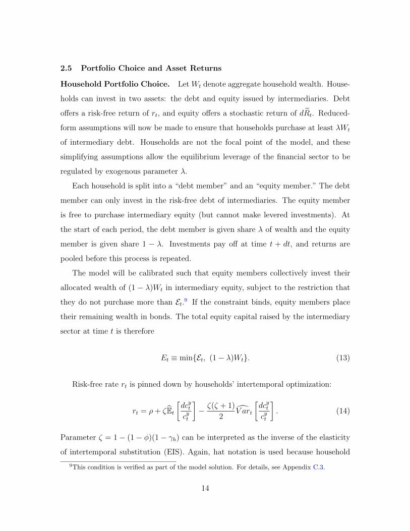
Risk-free rate rt is pinned down by households’ intertemporal optimization:
rt = ρ+ ζEt[dcytcyt
]− ζ(ζ + 1)
2V art
[dcytcyt
]. (14)
Parameter ζ = 1− (1− φ)(1− γh) can be interpreted as the inverse of the elasticity
of intertemporal substitution (EIS). Again, hat notation is used because household
9This condition is verified as part of the model solution. For details, see Appendix C.3.
14
expectations of the consumption process are diagnostic. Equation (14) is the standard
consumption-based risk-free rate formula in continuous time.10
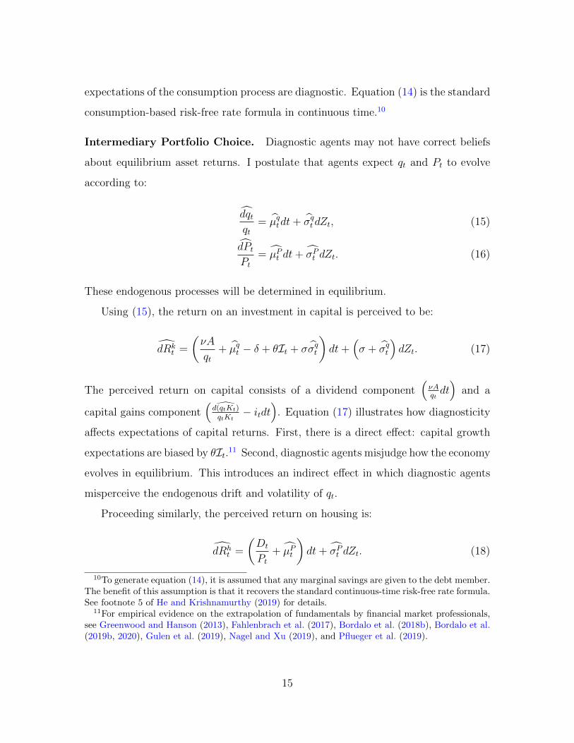
Intermediary Portfolio Choice. Diagnostic agents may not have correct beliefs
about equilibrium asset returns. I postulate that agents expect qt and Pt to evolve
according to:
dqtqt
= µqtdt+ σqt dZt, (15)
dPtPt
= µPt dt+ σPt dZt. (16)
These endogenous processes will be determined in equilibrium.
Using (15), the return on an investment in capital is perceived to be:
dRkt =
(νA
qt+ µqt − δ + θIt + σσqt
)dt+
(σ + σqt
)dZt. (17)
The perceived return on capital consists of a dividend component(νAqtdt)
and a
capital gains component( d(qtKt)
qtKt− itdt
). Equation (17) illustrates how diagnosticity
affects expectations of capital returns. First, there is a direct effect: capital growth
expectations are biased by θIt.11 Second, diagnostic agents misjudge how the economy
evolves in equilibrium. This introduces an indirect effect in which diagnostic agents
misperceive the endogenous drift and volatility of qt.
Proceeding similarly, the perceived return on housing is:
dRht =
(Dt
Pt+ µPt
)dt+ σPt dZt. (18)
10To generate equation (14), it is assumed that any marginal savings are given to the debt member.The benefit of this assumption is that it recovers the standard continuous-time risk-free rate formula.See footnote 5 of He and Krishnamurthy (2019) for details.
11For empirical evidence on the extrapolation of fundamentals by financial market professionals,see Greenwood and Hanson (2013), Fahlenbrach et al. (2017), Bordalo et al. (2018b), Bordalo et al.(2019b, 2020), Gulen et al. (2019), Nagel and Xu (2019), and Pflueger et al. (2019).
15
The dividend on housing is given by rental income Dt. Price Pt is the present dis-
counted value of these cash flows. Diagnosticity biases expectations of housing rent
growth, which produces non-rational expectations of price process Pt.
Let πkt ≡(νAqt
+ µqt − δ + θIt + σσqt
)− rt denote the perceived risk premium on
capital. Let πht ≡(DtPt
+ µPt
)− rt denote the perceived risk premium on housing.
Equations (17) and (18) can be rewritten as follows:
dRkt =
(πkt + rt
)dt+ σkt dZt, and
dRht =
(πht + rt
)dt+ σht dZt,
where σkt ≡ σ + σqt and σht ≡ σPt .
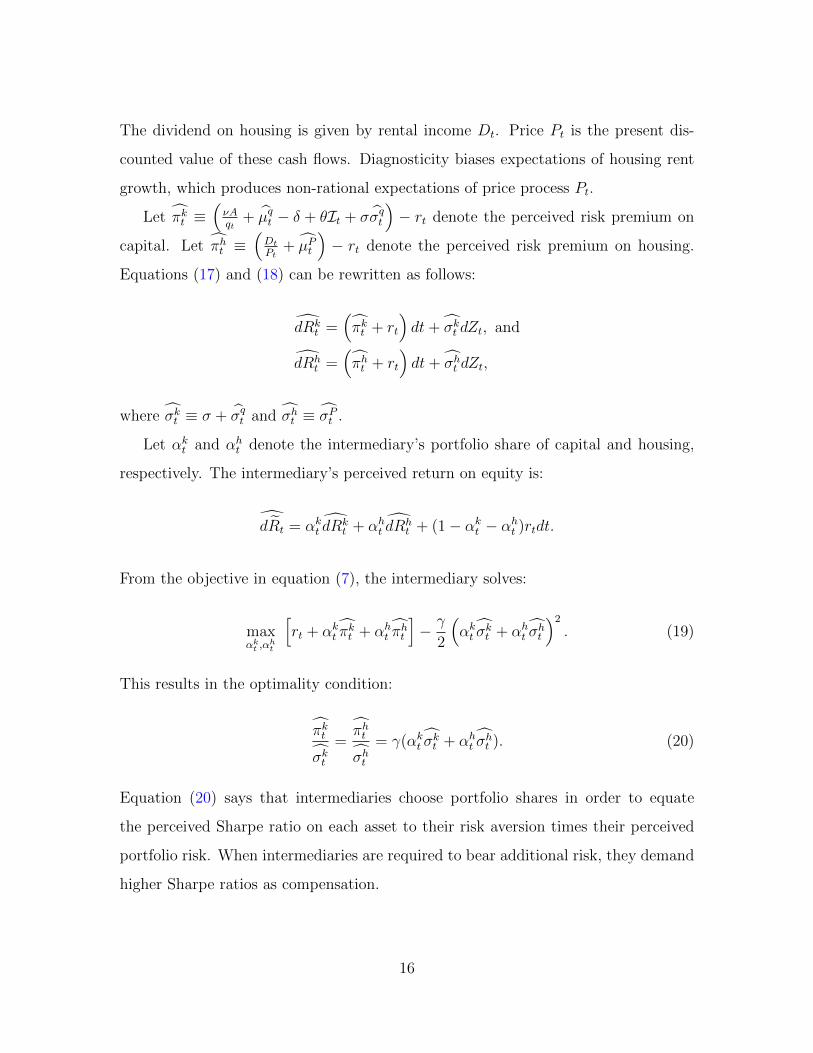
Let αkt and αht denote the intermediary’s portfolio share of capital and housing,
respectively. The intermediary’s perceived return on equity is:
dRt = αkt dRkt + αht dR
ht + (1− αkt − αht )rtdt.
From the objective in equation (7), the intermediary solves:
maxαkt ,α
ht
[rt + αkt π
kt + αht π
ht
]− γ
2
(αkt σ
kt + αht σ
ht
)2
. (19)
This results in the optimality condition:
πkt
σkt=πht
σht= γ(αkt σ
kt + αht σ
ht ). (20)
Equation (20) says that intermediaries choose portfolio shares in order to equate
the perceived Sharpe ratio on each asset to their risk aversion times their perceived
portfolio risk. When intermediaries are required to bear additional risk, they demand
higher Sharpe ratios as compensation.
16
2.6 Summary: Financial Frictions and Behavioral Frictions
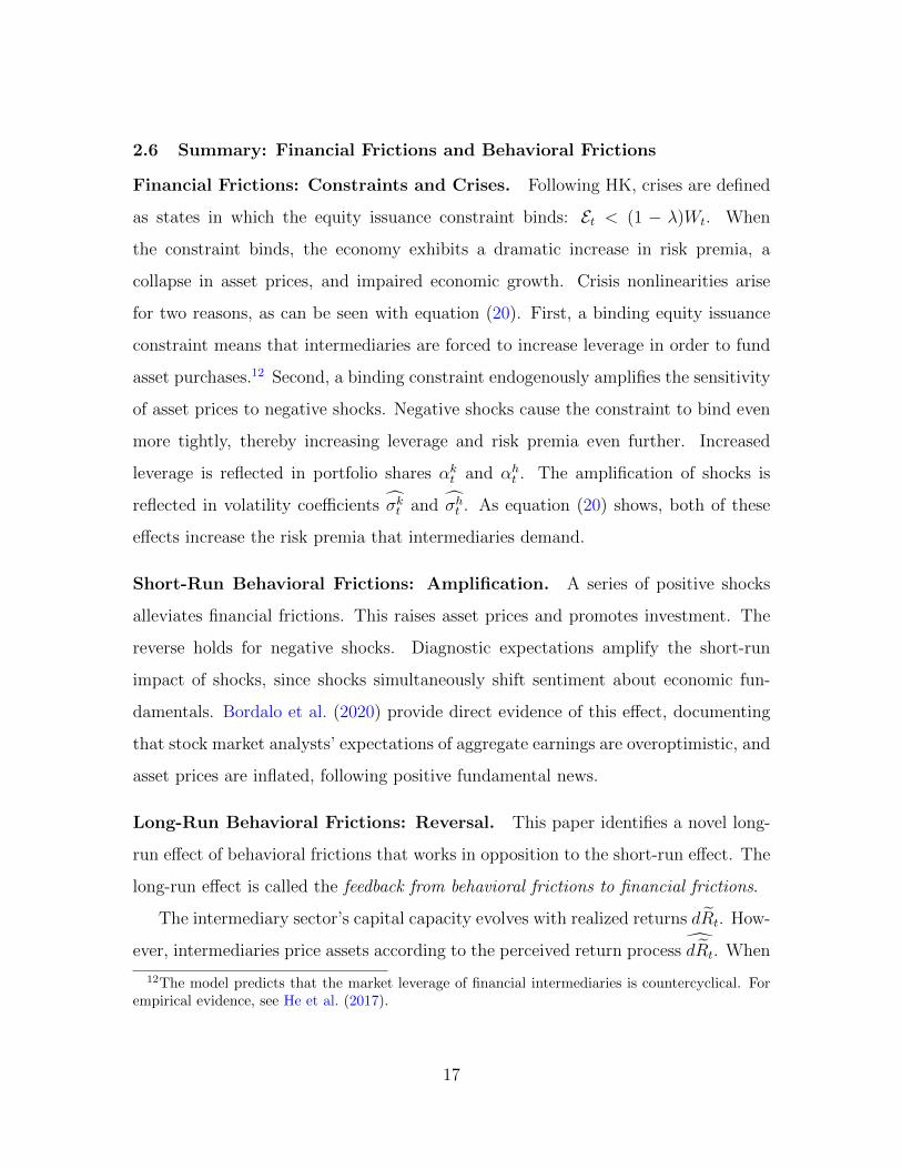
Financial Frictions: Constraints and Crises. Following HK, crises are defined
as states in which the equity issuance constraint binds: Et < (1 − λ)Wt. When
the constraint binds, the economy exhibits a dramatic increase in risk premia, a
collapse in asset prices, and impaired economic growth. Crisis nonlinearities arise
for two reasons, as can be seen with equation (20). First, a binding equity issuance
constraint means that intermediaries are forced to increase leverage in order to fund
asset purchases.12 Second, a binding constraint endogenously amplifies the sensitivity
of asset prices to negative shocks. Negative shocks cause the constraint to bind even
more tightly, thereby increasing leverage and risk premia even further. Increased
leverage is reflected in portfolio shares αkt and αht . The amplification of shocks is
reflected in volatility coefficients σkt and σht . As equation (20) shows, both of these
effects increase the risk premia that intermediaries demand.
Short-Run Behavioral Frictions: Amplification. A series of positive shocks
alleviates financial frictions. This raises asset prices and promotes investment. The
reverse holds for negative shocks. Diagnostic expectations amplify the short-run
impact of shocks, since shocks simultaneously shift sentiment about economic fun-
damentals. Bordalo et al. (2020) provide direct evidence of this effect, documenting
that stock market analysts’ expectations of aggregate earnings are overoptimistic, and
asset prices are inflated, following positive fundamental news.
Long-Run Behavioral Frictions: Reversal. This paper identifies a novel long-
run effect of behavioral frictions that works in opposition to the short-run effect. The
long-run effect is called the feedback from behavioral frictions to financial frictions.
The intermediary sector’s capital capacity evolves with realized returns dRt. How-
ever, intermediaries price assets according to the perceived return process dRt. When
12The model predicts that the market leverage of financial intermediaries is countercyclical. Forempirical evidence, see He et al. (2017).
17
the perceived return process differs from the true return process, market prices will
not reflect fundamentals. In the case of elevated sentiment, persistent forecast er-
rors lower realized returns and cause intermediaries’ capital capacity to deteriorate
relative to expectations. Thus, overoptimism induces a gradual tightening of finan-
cial frictions. Alternatively, excessive pessimism gradually relaxes financial frictions.
This long-run feedback from behavioral frictions to financial frictions will be a key
mechanism driving many of the model’s main predictions.
3 Equilibrium and Model Calibration
3.1 Equilibrium
Definition 1. Diagnostic Expectations Equilibrium (DEE). A diagnostic ex-
pectations equilibrium is a set of prices {qt, Pt, Dt, rt,Wt} and decisions {cyt , cht , it, αkt , αht }
such that:
1. Given prices, decisions as specified by (10), (12), (14), and (19) are optimal
under diagnostic expectations.
2. The goods market and housing rental market clear (using Cy and Ch to indicate
aggregate household consumption):
Yt = AKt = Cyt + Φ(it, Kt), and (21)
Cht = H ≡ 1.
3. The equity issuance constraint is satisfied:
Et = min{Et, (1− λ)Wt}.
18
4. Asset markets clear with intermediaries holding all capital and housing:
qtKt = αktEt, and (22)
Pt = αhtEt. (23)
5. The total value of assets equals total household wealth:
Wt = qtKt + Pt.
Diagnostic expectations generalize rational expectations. Rationality is recovered
by setting θ = 0. This is formalized in the following definition, which will serve as a
benchmark for later comparison.
Definition 2. Rational Expectations Equilibrium (REE). A rational expecta-
tions equilibrium is a diagnostic expectations equilibrium for θ = 0.
Solution Strategy. I consider Markov equilibria in state variables Kt, Et, and It.
Kt scales the size of the economy, Et is the financial sector’s capital capacity, and Itcharacterizes sentiment. HK use Kt and Et as state variables in their rational model.
The innovation of this paper is to capture behavioral frictions with state variable It.
When expectations are extrapolative it is not enough to know the current state of
the economy (Kt and Et); one must also know the path taken to get there (It).
The solution can be simplified further by scaling the economy by Kt. Define
et ≡EtKt
.
et captures the capital capacity of the intermediary sector relative to the size of
the overall economy. I look for price functions of the form pt = PtKt
= p(et, It)
and qt = q(et, It). The model is solved numerically as a function of et and It: et
characterizes financial frictions, and It characterizes behavioral frictions.
19
In the class of Markov equilibria considered here, each diagnostic expectations
equilibrium nests its corresponding rational expectations equilibrium. When solving
for a DEE, this means that the REE comes “for free.” Formally:
Proposition 1. For any DEE that is Markov in {K, e, I}, the price and policy func-
tions for {K, e, I = 0} compose a REE that is Markov in {K, e}.
Proof. Equation (4) specifies that when It = 0, agents act as if I = 0 in perpetuity.
Decisions that are optimal when I = 0 in perpetuity must also be optimal when θ = 0
(REE), because in both cases I is perceived to have no further effect on the resulting
equilibrium.
3.2 Calibration
The HK model is a standard RBC model augmented with a financial intermediary
sector. The economy behaves like an RBC model when et is far from the constraint,
and intermediary frictions become quantitatively important near the crisis region. I
follow HK in defining edistress as the 33rd percentile value of et in the model’s stationary
distribution. edistress separates “normal” periods from periods of financial distress.
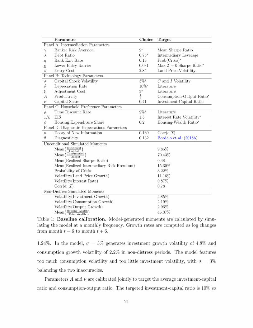
Table 1 presents the baseline calibration. I use the parameters and/or calibration
targets of He and Krishnamurthy (2019) when possible. Parameter values that are
marked with an asterisk in the “Choice” column are equivalent to the parameter
values of HK. Asterisks in the “Target” column indicate parameters for which the
value differs from HK, but the target is the same. The only parameters for which
neither the value nor the target aligns with HK are the three new parameters. These
are behavioral parameters θ and κ, and labor income parameter ν.
RBC Parameters. Discount rate ρ, depreciation rate δ, and adjustment cost ξ are
relatively standard RBC parameters. My calibration follows HK.
Parameter σ governs the volatility of capital quality shocks. As in HK, I set
σ = 3%. HK report that from 1975 to 2015 the volatility of investment growth
in non-distress periods was 5.79%, and the volatility of consumption growth was
20
Parameter Choice TargetPanel A: Intermediation Parametersγ Banker Risk Aversion 2∗ Mean Sharpe Ratioλ Debt Ratio 0.75∗ Intermediary Leverageη Bank Exit Rate 0.13 Prob(Crisis)∗
e Lower Entry Barrier 0.081 Max I = 0 Sharpe Ratio∗
β Entry Cost 2.8∗ Land Price VolatilityPanel B: Technology Parametersσ Capital Shock Volatility 3%∗ C and I Volatilityδ Depreciation Rate 10%∗ Literatureξ Adjustment Cost 3∗ LiteratureA Productivity 1
3Consumption-Output Ratio∗
ν Capital Share 0.41 Investment-Capital RatioPanel C: Household Preference Parametersρ Time Discount Rate 2%∗ Literature1/ζ EIS 1.5 Interest Rate Volatility∗
φ Housing Expenditure Share 0.2 Housing-Wealth Ratio∗
Panel D: Diagnostic Expectations Parametersκ Decay of New Information 0.139 Corr(e, I)θ Diagnosticity 0.132 Bordalo et al. (2018b)
Unconditional Simulated MomentsMean
(Investment
Capital
)9.85%
Mean(
ConsumptionOutput
)70.43%
Mean(Realized Sharpe Ratio) 0.48Mean(Realized Intermediary Risk Premium) 15.30%Probability of Crisis 3.22%Volatility(Land Price Growth) 11.16%Volatility(Interest Rate) 0.87%Corr(e, I) 0.78
Non-Distress Simulated MomentsVolatility(Investment Growth) 4.85%Volatility(Consumption Growth) 2.19%Volatility(Output Growth) 2.96%
Mean(
Housing WealthTotal Wealth
)45.37%
Table 1: Baseline calibration. Model-generated moments are calculated by simu-lating the model at a monthly frequency. Growth rates are computed as log changesfrom month t− 6 to month t+ 6.
1.24%. In the model, σ = 3% generates investment growth volatility of 4.8% and
consumption growth volatility of 2.2% in non-distress periods. The model features
too much consumption volatility and too little investment volatility, with σ = 3%
balancing the two inaccuracies.
Parameters A and ν are calibrated jointly to target the average investment-capital
ratio and consumption-output ratio. The targeted investment-capital ratio is 10% so
21
that average investment matches depreciation. Since the dividend yield on capi-
tal is νAqt
, ν and A are calibrated to generate a capital price q commensurate with
a 10% investment-capital ratio. To separately identify A and ν, I also target an
average consumption-output ratio of 70%. The consumption-output ratio equals
AKt−Φ(it,Kt)AKt
≈ 1− itA
. An investment-capital ratio of 10% pins down A = 13.
Intermediation Parameters. Parameter γ represents the bankers’ risk aversion.
As in HK, I set γ = 2. This generates an average realized Sharpe ratio of 0.48, and
an average realized intermediary risk premium of 15.30%. This aligns with He et al.
(2017), who estimate an average Sharpe ratio of 0.48 and an average return of 13%
for assets intermediated by the financial sector.
Intermediary leverage is governed by λ. Since intermediaries have assets of Pt +
qtKt = Wt and equity of Et, equation (13) gives a market leverage value of Wt
Et= 1
1−λ
in non-crisis states. Again following HK, I set λ = 0.75. This generates a leverage
ratio of 4 when the constraint does not bind.
Crisis Parameters. Crises are defined as states in which the equity issuance con-
straint binds. Bank exit rate η targets a 3% crisis probability.
Parameters e and β control the lower boundary condition, represented by dψt in
equation (8) (details in Appendix B.4). Parameter e is the minimum level of capital
capacity at which new entry occurs, and β is the cost of entry into the intermediary
sector. HK set e such that the Sharpe ratio at e is 6.5 (e is set low enough that entry
occurs rarely). Accordingly, I set e such that the perceived Sharpe ratio at e and
I = 0 is 6.5. Parameter β determines the slope of house price Pt at e, which in turn
affects the volatility of Pt throughout the distress region. As in HK, I set β = 2.8.
HK estimate that the empirical volatility of land price growth from 1975 to 2015 is
11.9%. In the model, β = 2.8 generates land price growth volatility of 11.2%.
Household Parameters. Parameter φ governs the relative value of housing ser-
vices to the output good. This determines the rental rate Dt (see equation (10)). Pt
22
is the discounted value of these rental payments. I set φ = 0.2 to target a non-distress
housing-wealth ratio of 45%. φ = 0.2 also generates a housing services to total con-
sumption expenditure ratio that is consistent with NIPA consumption data (Davis
and Van Nieuwerburgh, 2015).
ζ is the inverse of the EIS, and determines the responsiveness of the risk-free rate
to expected consumption growth and volatility. When expectations are diagnostic,
agents misperceive the equilibrium consumption process. Thus, ζ also governs the
sensitivity of the risk-free rate to variation in sentiment. The EIS plays an important
role when expectations are diagnostic, because the EIS regulates the extent to which
sentiment gets incorporated into asset prices. When ζ = 1, any bias in growth expec-
tations is passed one-for-one into discount rate rt (see equation (14)). An important
implication is that when ζ = 1, asset prices qt and Pt are independent of It — all
bias in cash-flow expectations is exactly offset by the risk-free rate. When ζ < 1, rt
responds less than one-for-one to biased growth expectations. In this case, qt and Pt
are increasing in It.
I set the EIS equal to 1.5. This is a standard choice in the finance literature
(e.g., Bansal and Yaron, 2004), and, as in HK, generates real interest rate volatility
of roughly 1%. Since ζ < 1, asset prices are increasing in It. This will be important
for generating the results in Section 5.2.
Behavioral Parameters. θ governs the extent to which expectations are biased
by representativeness. κ governs the persistence of sentiment. θ and κ are calibrated
jointly using two targets. The first target aligns the magnitude of the expectations
bias with the estimates of Bordalo et al. (2018b): one standard deviation in sentiment
generates an output growth bias of 0.75 percentage points.13 The second target
matches the model’s unconditional correlation between state variables et and It to
the correlation between intermediary capital and sentiment estimated empirically.
To estimate this correlation in the data, I measure et with the “Intermediary Capital
13Note that V ar(θIt) = θ2σ2
2κ . This calibration target sets θ σ√2κ
= 0.0075.
23
Ratio” of He et al. (2017). It can be calculated using expectations data, given κ and
θ. Full calibration details are provided in Appendix A.2.
These two calibration targets produce θ = 0.132 and κ = 0.139. κ = 0.139 implies
that sentiment is slow moving, with a half-life of 5 years.14 Slow-moving sentiment
captures prolonged periods of relatively positive and negative news, such as the Great
Moderation, rather than high-frequency volatility.15 Appendix B.6 examines robust-
ness to parameters κ, θ, and ζ.
4 Global Solution
4.1 Prices, Policy Functions, and Forecast Errors
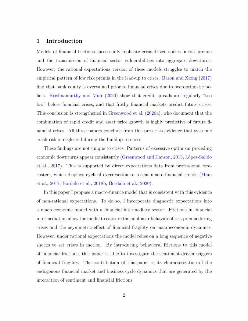
Select price and policy functions for the DEE are shown in Figure 2.16 The horizontal
axis lists capital capacity e = EK
. All panels plot three curves. The blue curve
corresponds to depressed sentiment (I = −1.5SD), the red curve corresponds to
neutral sentiment (I = 0), and the yellow curve corresponds to elevated sentiment
(I = +1.5SD).
The two leftmost panels of Figure 2 show asset prices q(e, I) and p(e, I). Finan-
cial frictions make asset prices sensitive to capital capacity e. In the crisis region
(approximately e < 0.4), the binding constraint causes asset prices to plummet. The
Sharpe ratio panels illustrate the nonlinear spike in risk premia that characterizes
crisis times. Moving right, asset prices rise as intermediaries’ risk-bearing capacity
increases. Asset prices asymptote for high values of e as financial frictions dissipate.
Asset prices exhibit what HK refer to as “anticipation effects”: asset prices start
to fall well before the equity issuance constraint binds. Anticipation effects arise in
equilibrium because forward-looking intermediaries are unwilling to support elevated
asset prices in the face of mounting systemic risk.17 Anticipation effects mean that
14Using a different specification than this paper, Bordalo et al. (2019b) estimate that the diagnosticexpectations of stock market analysts incorporate the past three years of shocks.
15The beliefs model can be extended such that sentiment contains both a slow-moving componentand a high-frequency component. However, this requires an additional state variable.
16See Appendix Figure 6 for more.17Intermediaries perceive that risk premia will be low when asset prices are high, and vice-versa.
24
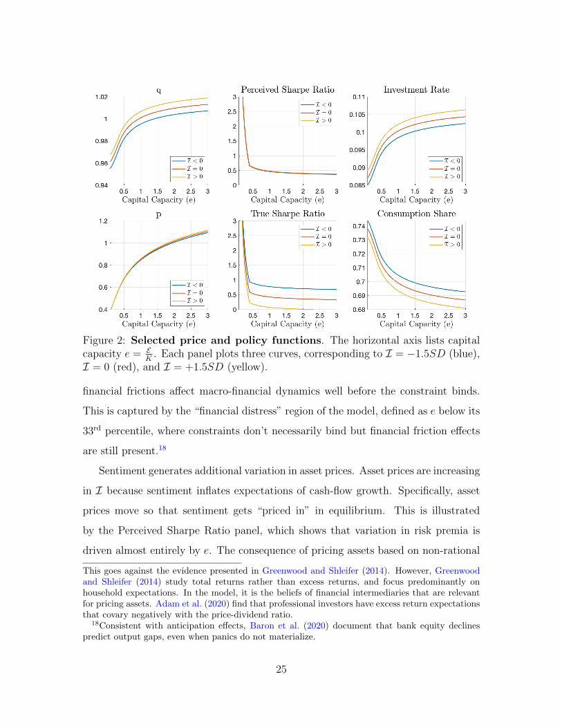
Figure 2: Selected price and policy functions. The horizontal axis lists capitalcapacity e = E
K. Each panel plots three curves, corresponding to I = −1.5SD (blue),
I = 0 (red), and I = +1.5SD (yellow).
financial frictions affect macro-financial dynamics well before the constraint binds.
This is captured by the “financial distress” region of the model, defined as e below its
33rd percentile, where constraints don’t necessarily bind but financial friction effects
are still present.18
Sentiment generates additional variation in asset prices. Asset prices are increasing
in I because sentiment inflates expectations of cash-flow growth. Specifically, asset
prices move so that sentiment gets “priced in” in equilibrium. This is illustrated
by the Perceived Sharpe Ratio panel, which shows that variation in risk premia is
driven almost entirely by e. The consequence of pricing assets based on non-rational
This goes against the evidence presented in Greenwood and Shleifer (2014). However, Greenwoodand Shleifer (2014) study total returns rather than excess returns, and focus predominantly onhousehold expectations. In the model, it is the beliefs of financial intermediaries that are relevantfor pricing assets. Adam et al. (2020) find that professional investors have excess return expectationsthat covary negatively with the price-dividend ratio.
18Consistent with anticipation effects, Baron et al. (2020) document that bank equity declinespredict output gaps, even when panics do not materialize.
25
expectations is shown in the True Sharpe Ratio panel. Elevated sentiment lowers
realized risk premia, while depressed sentiment raises realized risk premia.
The investment and consumption panels show the propagation of financial and
behavioral frictions to the real economy. The investment rate is high whenever either
e or I is high. The consumption share Cy
Ymoves in the opposite manner. This follows
from output market clearing in equation (21).
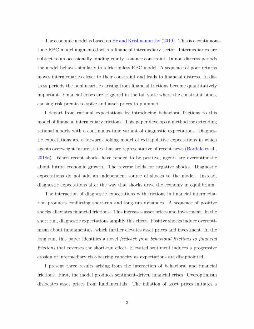
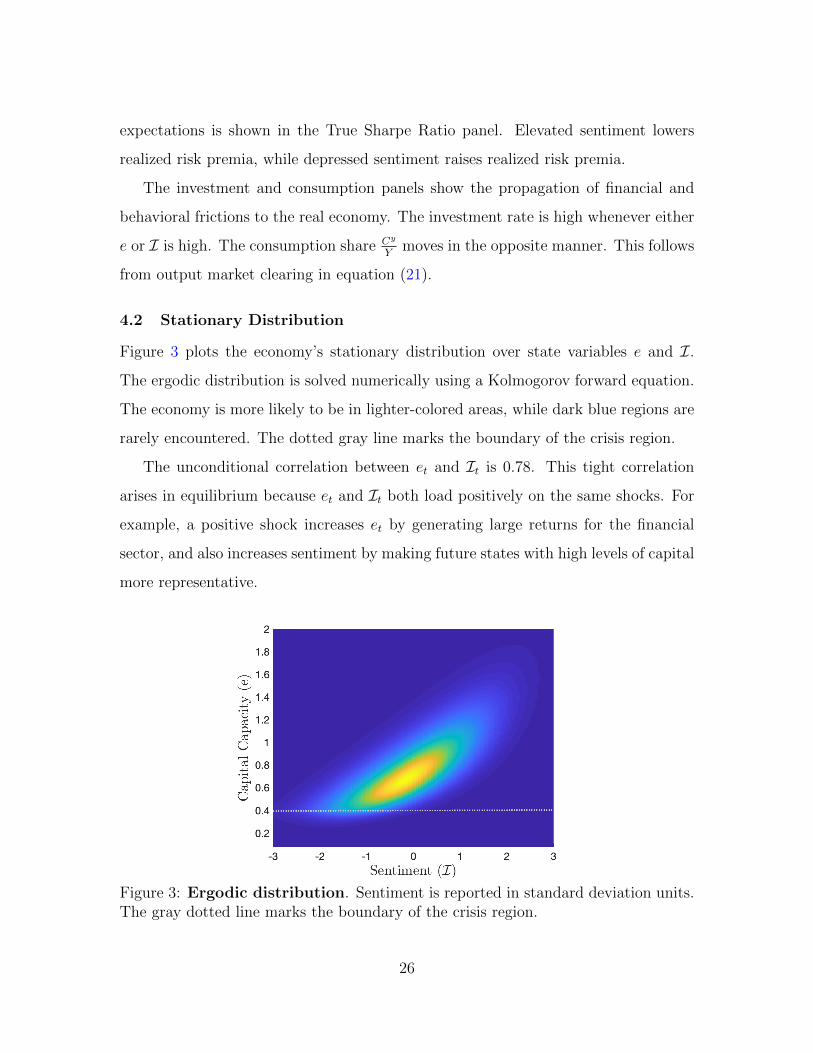
4.2 Stationary Distribution
Figure 3 plots the economy’s stationary distribution over state variables e and I.
The ergodic distribution is solved numerically using a Kolmogorov forward equation.
The economy is more likely to be in lighter-colored areas, while dark blue regions are
rarely encountered. The dotted gray line marks the boundary of the crisis region.
The unconditional correlation between et and It is 0.78. This tight correlation
arises in equilibrium because et and It both load positively on the same shocks. For
example, a positive shock increases et by generating large returns for the financial
sector, and also increases sentiment by making future states with high levels of capital
more representative.
Figure 3: Ergodic distribution. Sentiment is reported in standard deviation units.The gray dotted line marks the boundary of the crisis region.
26
5 Results: Financial Market and Macroeconomic Dynamics
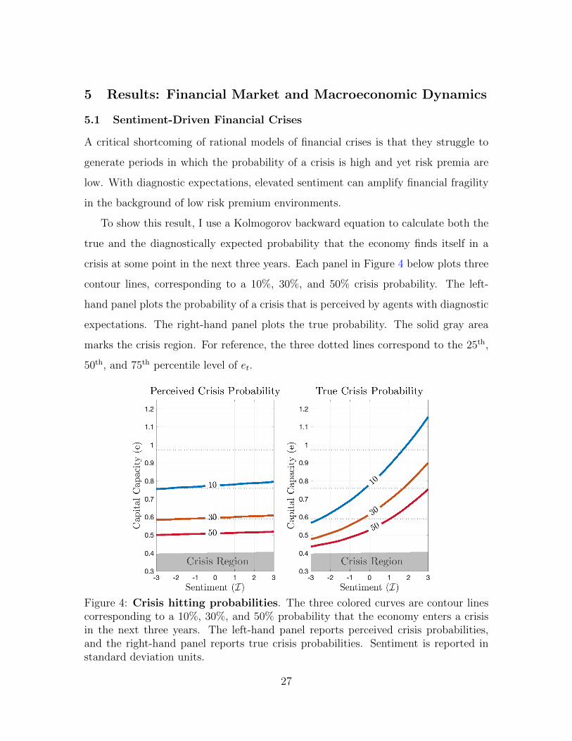
5.1 Sentiment-Driven Financial Crises
A critical shortcoming of rational models of financial crises is that they struggle to
generate periods in which the probability of a crisis is high and yet risk premia are
low. With diagnostic expectations, elevated sentiment can amplify financial fragility
in the background of low risk premium environments.
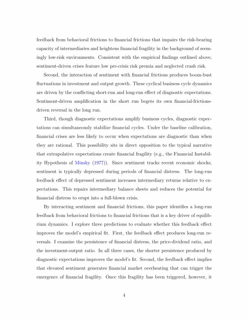
To show this result, I use a Kolmogorov backward equation to calculate both the
true and the diagnostically expected probability that the economy finds itself in a
crisis at some point in the next three years. Each panel in Figure 4 below plots three
contour lines, corresponding to a 10%, 30%, and 50% crisis probability. The left-
hand panel plots the probability of a crisis that is perceived by agents with diagnostic
expectations. The right-hand panel plots the true probability. The solid gray area
marks the crisis region. For reference, the three dotted lines correspond to the 25th,
50th, and 75th percentile level of et.
Figure 4: Crisis hitting probabilities. The three colored curves are contour linescorresponding to a 10%, 30%, and 50% probability that the economy enters a crisisin the next three years. The left-hand panel reports perceived crisis probabilities,and the right-hand panel reports true crisis probabilities. Sentiment is reported instandard deviation units.
27
Sentiment has almost no impact on perceived crisis probabilities.19 Diagnostic
expectations of fundamentals are incorporated into prices, so intermediaries perceive
that crash risk is driven almost entirely by et. Perceived crash risk is high only near
the crisis region, and fragility is quickly attenuated as the financial sector strengthens
its capital capacity.
In the right-hand panel, the tilting of the contour lines highlights the buildup of
undetected systemic risk that is triggered by overoptimism. When It > 0, interme-
diaries borrow at elevated interest rates and pay inflated prices to purchase capital
and housing. As expectations disappoint, the feedback from behavioral frictions to
financial frictions causes intermediary balance sheets to deteriorate. Because this
heightened fragility is an endogenous consequence of overoptimistic beliefs, it is ne-
glected by intermediaries. Thus, diagnostic expectations allow the model to generate
periods in which actual crash risk is high and yet risk premia are low.
The reverse story explains why perceived crisis probabilities are too high when
It < 0. Excessive pessimism allows the intermediary sector to borrow at low interest
rates and purchase assets cheaply. When cash flows end up being larger than expected,
the feedback effect works in the opposite direction and intermediaries quickly rebuild
their capital capacity.
Figure 4 shows that when expectations are diagnostic, periods in which interme-
diary balance sheets appear to be strong can still be associated with heightened crisis
risk. For example, when I = 0 and the intermediary sector is at its median level
of capital capacity, the three-year crisis probability is roughly 10%. This probability
jumps to 30% when sentiment is elevated by 1.5 standard deviations. This result
aligns with Greenwood et al. (2020b), who estimate that the three-year probability of
a crisis reaches 40% when financial fragility is accompanied by elevated asset prices.
19Perceived crisis probabilities slope upward slightly. The reason is that a crisis is defined aset < (1− λ)(pt + qt) (see equation (13)). Since the right-hand side of this inequality is increasing insentiment, a given level of et is closer to the crisis region when It is high.
28
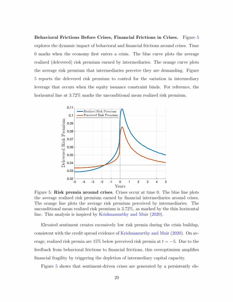
Behavioral Frictions Before Crises, Financial Frictions in Crises. Figure 5
explores the dynamic impact of behavioral and financial frictions around crises. Time
0 marks when the economy first enters a crisis. The blue curve plots the average
realized (delevered) risk premium earned by intermediaries. The orange curve plots
the average risk premium that intermediaries perceive they are demanding. Figure
5 reports the delevered risk premium to control for the variation in intermediary
leverage that occurs when the equity issuance constraint binds. For reference, the
horizontal line at 3.72% marks the unconditional mean realized risk premium.
Figure 5: Risk premia around crises. Crises occur at time 0. The blue line plotsthe average realized risk premium earned by financial intermediaries around crises.The orange line plots the average risk premium perceived by intermediaries. Theunconditional mean realized risk premium is 3.72%, as marked by the thin horizontalline. This analysis is inspired by Krishnamurthy and Muir (2020).
Elevated sentiment creates excessively low risk premia during the crisis buildup,
consistent with the credit spread evidence of Krishnamurthy and Muir (2020). On av-
erage, realized risk premia are 15% below perceived risk premia at t = −5. Due to the
feedback from behavioral frictions to financial frictions, this overoptimism amplifies
financial fragility by triggering the depletion of intermediary capital capacity.
Figure 5 shows that sentiment-driven crises are generated by a persistently ele-
29
vated level of sentiment, not a sudden and dramatic change of sentiment. In fact,
realized risk premia catch up to perceived risk premia approximately 1.5 years before
crises hit, a pattern also shown in Krishnamurthy and Muir (2020). More broadly,
this aligns with an emerging empirical finding that crises are the result of a slow-
building erosion of financial sector resilience rather than a sudden sentiment shock
(Baron et al., 2020).
The spike at t = 0 illustrates that both behavioral frictions and financial fric-
tions are needed to replicate the full path of risk premia around crises. Diagnostic
expectations produce low pre-crisis risk premia and neglected crash risk. However,
slow-moving sentiment alone cannot generate the spike in risk premia caused by the
binding constraint. Ex-ante behavioral frictions set the stage for crisis nonlinearities
driven by financial frictions.
The model’s post-crisis patterns reverse those of the pre-crisis period. The post-
crisis period is characterized by excessive pessimism. Risk premia therefore sit above
fundamentals in the aftermath of crises.20
5.2 Boom-Bust Investment Cycles
I now turn to studying sentiment-driven macroeconomic fluctuations. Diagnostic ex-
pectations affect investment rate it, which in turn controls the growth rate of output:
dYtYt
= (it − δ)dt+ σdZt.
Before proceeding, I emphasize that the calibration of ζ is important here. ζ
governs how diagnostic expectations are passed into asset prices versus the risk-free
rate. The baseline calibration sets ζ < 1. This means that qt is increasing in It.
Accordingly, it is also increasing in sentiment.
I use impulse-response functions to study the response of investment to economic
shocks. To capture periods of booms and malaise, I simulate the model at a monthly
frequency and feed in a three-year sequence of either positive or negative shocks.
These monthly shocks result in a one standard deviation cumulative shock over three
20See Muir (2017) for empirical evidence of high post-crisis risk premia.
30
years.21 Shocks are turned off thereafter.
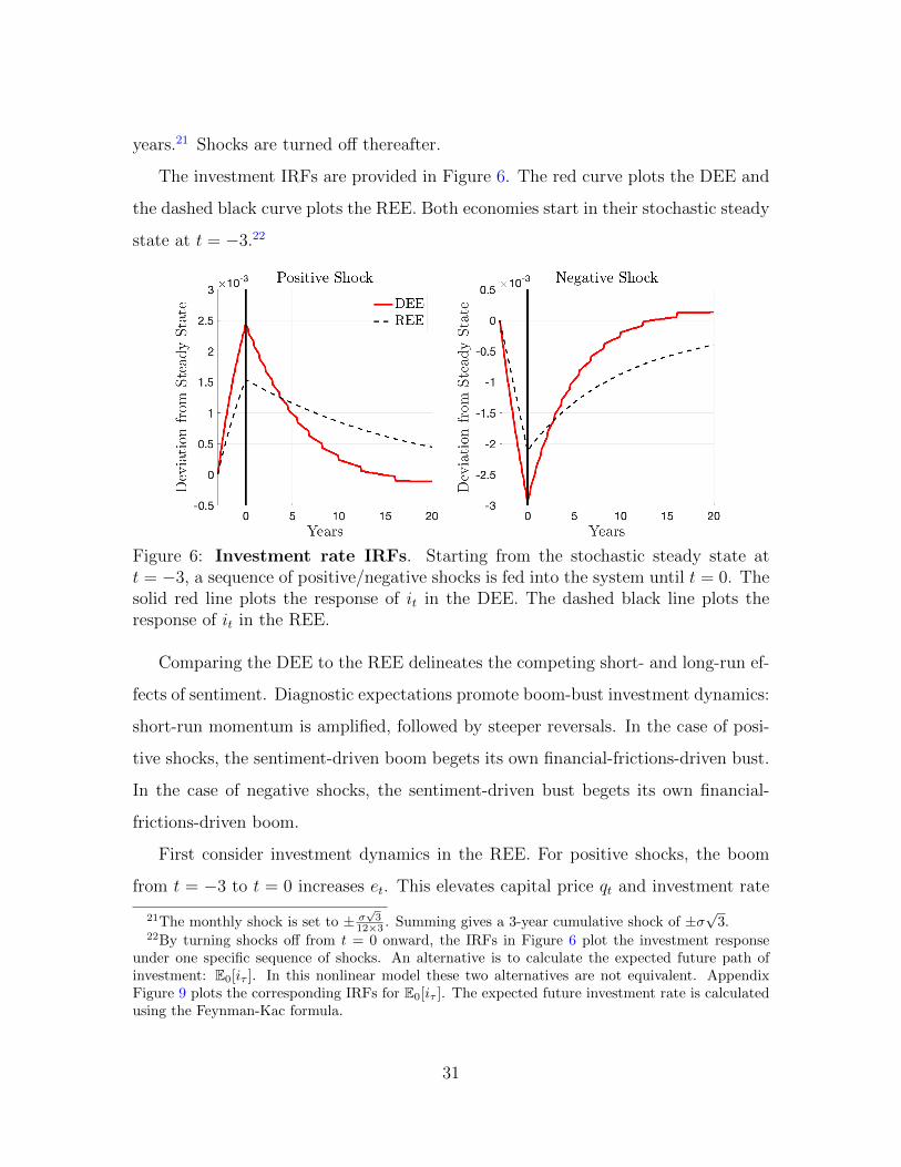
The investment IRFs are provided in Figure 6. The red curve plots the DEE and
the dashed black curve plots the REE. Both economies start in their stochastic steady
state at t = −3.22
Figure 6: Investment rate IRFs. Starting from the stochastic steady state att = −3, a sequence of positive/negative shocks is fed into the system until t = 0. Thesolid red line plots the response of it in the DEE. The dashed black line plots theresponse of it in the REE.
Comparing the DEE to the REE delineates the competing short- and long-run ef-
fects of sentiment. Diagnostic expectations promote boom-bust investment dynamics:
short-run momentum is amplified, followed by steeper reversals. In the case of posi-
tive shocks, the sentiment-driven boom begets its own financial-frictions-driven bust.
In the case of negative shocks, the sentiment-driven bust begets its own financial-
frictions-driven boom.
First consider investment dynamics in the REE. For positive shocks, the boom
from t = −3 to t = 0 increases et. This elevates capital price qt and investment rate
21The monthly shock is set to ± σ√
312×3 . Summing gives a 3-year cumulative shock of ±σ
√3.
22By turning shocks off from t = 0 onward, the IRFs in Figure 6 plot the investment responseunder one specific sequence of shocks. An alternative is to calculate the expected future path ofinvestment: E0[iτ ]. In this nonlinear model these two alternatives are not equivalent. AppendixFigure 9 plots the corresponding IRFs for E0[iτ ]. The expected future investment rate is calculatedusing the Feynman-Kac formula.
31
it. Since et and it are both above their steady-state levels when the shocks stop at
t = 0, they proceed to drift slowly back to the steady state. The opposite holds for
negative shocks.
Turning to the DEE, consider the boom-bust pattern of the positive shock case.
Positive shocks from t = −3 to t = 0 elevate It in addition to et. This causes a sharper
investment boom in the short run. However, the feedback from behavioral frictions to
financial frictions implies that excessive optimism decreases the subsequent returns
earned by intermediaries. Over time, this erodes intermediary balance sheets and
reduces long-run investment.
The negative shock case produces a bust-boom pattern in the DEE. Negative
shocks depress sentiment, which amplifies the short-run drop in investment. But, the
sentiment-driven bust also increases the future returns earned by intermediaries. As
sentiment recovers, the economy is left with a stronger financial sector that is able to
support higher levels of investment.23
Appendix Figure 7 studies the IRFs of an economy with diagnostic expectations
but without financial frictions. Alone, slow-moving diagnostic expectations do not
generate steep reversals in investment. The long-run reversals shown in Figure 6 rely
on the feedback from behavioral frictions to financial frictions.
Recent empirical evidence supports the pattern of boom-bust investment cycles.
Gulen et al. (2019) find that elevated credit-market sentiment in year t correlates with
a boom in corporate investment over the subsequent year, followed by a long-run con-
traction. Lopez-Salido et al. (2017) estimate that elevated credit-market sentiment in
year t predicts lower GDP growth in year t+2. The long-run feedback from behavioral
frictions to financial frictions is also consistent with the observation of Greenwood et
al. (2019) that financial fragility arises at the end of economic expansions.
23Figure 6 shows a mildly asymmetric investment response to positive versus negative shocks.Larger initial shocks produce larger asymmetries. This is illustrated in Appendix Figure 8, whichplots the IRFs that result after doubling the magnitude of the initial impulse.
32
5.3 Financial Market Stability from Beliefs
This paper identifies a stabilizing role for beliefs. Under the baseline calibration,
financial crises are less likely to occur when expectations are diagnostic than when
expectations are rational.
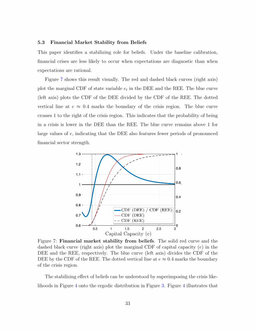
Figure 7 shows this result visually. The red and dashed black curves (right axis)
plot the marginal CDF of state variable et in the DEE and the REE. The blue curve
(left axis) plots the CDF of the DEE divided by the CDF of the REE. The dotted
vertical line at e ≈ 0.4 marks the boundary of the crisis region. The blue curve
crosses 1 to the right of the crisis region. This indicates that the probability of being
in a crisis is lower in the DEE than the REE. The blue curve remains above 1 for
large values of e, indicating that the DEE also features fewer periods of pronounced
financial sector strength.
Figure 7: Financial market stability from beliefs. The solid red curve and thedashed black curve (right axis) plot the marginal CDF of capital capacity (e) in theDEE and the REE, respectively. The blue curve (left axis) divides the CDF of theDEE by the CDF of the REE. The dotted vertical line at e ≈ 0.4 marks the boundaryof the crisis region.
The stabilizing effect of beliefs can be understood by superimposing the crisis like-
lihoods in Figure 4 onto the ergodic distribution in Figure 3. Figure 4 illustrates that
33
the joint occurrence of financial distress and elevated sentiment is highly predictive
of future financial crises. But, the ergodic distribution shows that this part of the
state space is rarely encountered. Instead, financial distress typically coincides with
excessive pessimism. When sentiment is pessimistic, the long-run reversal effect of
diagnostic expectations protects intermediaries from financial crises.
Financial market stability may appear at odds with the earlier results of this
paper. For example, Section 5.2 documents that diagnostic expectations amplify
business cycles. The finding here is that diagnostic expectations stabilize financial
markets. These results are intimately linked: the way that the economy avoids a
financial crisis is by going through a sentiment-driven recession. In the case of negative
shocks, depressed sentiment amplifies the investment bust in the short run. However,
the long-run reversal effect means that depressed sentiment simultaneously reduces
systemic risk by increasing the subsequent returns earned by intermediaries.
This finding of financial market stability may also appear to contradict the earlier
result of sentiment-driven crises. Indeed, much of the empirical literature has found
that elevated sentiment is predictive of financial market downturns, and concluded
from this finding that extrapolative expectations promote financial instability. The
model shows that such a conclusion does not necessarily follow from the evidence of
sentiment-driven crises.
To reconcile sentiment-driven crises with financial market stability, note that the
former is a conditional prediction while the latter is an unconditional prediction. The
model’s conditional prediction is that systemic risk is amplified when financial distress
and elevated sentiment occur jointly. However, it is rare for the economy to reach
these fragile states. The model’s unconditional prediction is that beliefs can stabilize
the financial sector, because financial distress is strongly correlated with depressed
sentiment.
The goal of this section is not to assert that extrapolative expectations necessarily
create financial stability. Rather, this section shows that the stabilizing effect of
34
extrapolation is a legitimate theoretical possibility, and one that the literature has
neglected to date. Though diagnostic expectations prevent financial crises under
the baseline calibration, this result can be overturned under alternate calibrations
in which the magnitude of perceptual error is increased. Robustness is explored in
Appendix B.6.
The identification of a stabilizing role for beliefs highlights a benefit of economic
models. The model can be used to compare outcomes from different data generating
processes (DEE versus REE). For the same reason, it is difficult to provide direct
empirical evidence on financial market stability from beliefs. Nonetheless, expecta-
tions data is consistent with the channel of unanticipated reversals in financial market
conditions. Bordalo et al. (2018a) analyze professional forecasts of the Baa-Treasury
credit spread, finding that periods of financial distress reverse faster than forecast-
ers expect. Similarly, Pflueger et al. (2019) document that market risk mean-reverts
faster than analysts, options prices, and loan officers expect.
6 Evaluating Diagnosticity: The Feedback Effect
The feedback from behavioral frictions to financial frictions is a key mechanism un-
derlying the model’s equilibrium dynamics. This section tests three predictions that
arise from this feedback. First, the feedback effect produces long-run reversals in
economic conditions. This implies that the economy exhibits less persistence under
diagnostic expectations than under rational expectations. Second, I use the model’s
prediction about how behavioral and financial frictions interact to identify a new fact
about which crises are preceded by frothy financial markets. Third, I apply the model
to the 2007-2008 Financial Crisis in order to assess the role of diagnostic expectations
in shaping the evolution of the crisis.
6.1 Prediction 1: Long-Run Reversals and Economic Persistence
I start by comparing the persistence of macro-financial processes in the model and
the data. Since the model’s calibration does not target measures of persistence ex-
35
plicitly, an indicator of success is the extent to which the long-run reversals channel
of diagnostic expectations helps to align the model with empirical moments.
In the experiments below, the calibration of the REE is identical to the calibration
of the DEE, except for θ = 0. I choose not to recalibrate the REE in order to pinpoint
the effect of θ. Results are essentially unchanged if the REE is recalibrated (see
Appendix B.7).
The Persistence of Financial Fragility. I begin by comparing the persistence
of financial fragility in the DEE and the REE. The long-run reversal channel of diag-
nostic expectations means that intermediaries will recover from financial crises more
quickly under diagnostic expectations than under rational expectations. Since crises
are generated by a sequence of negative shocks, sentiment in the DEE is typically
overpessimistic following crises. Due to the feedback from behavioral frictions to fi-
nancial frictions, excessive pessimism stimulates intermediaries’ recovery from crises.
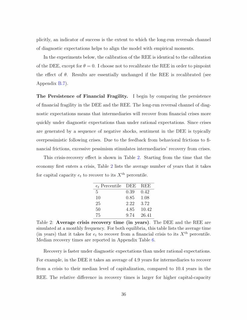
This crisis-recovery effect is shown in Table 2. Starting from the time that the
economy first enters a crisis, Table 2 lists the average number of years that it takes
for capital capacity et to recover to its Xth percentile.
et Percentile DEE REE5 0.39 0.4210 0.85 1.0825 2.22 3.7250 4.85 10.4275 9.74 26.41
Table 2: Average crisis recovery time (in years). The DEE and the REE aresimulated at a monthly frequency. For both equilibria, this table lists the average time(in years) that it takes for et to recover from a financial crisis to its Xth percentile.Median recovery times are reported in Appendix Table 6.
Recovery is faster under diagnostic expectations than under rational expectations.
For example, in the DEE it takes an average of 4.9 years for intermediaries to recover
from a crisis to their median level of capitalization, compared to 10.4 years in the
REE. The relative difference in recovery times is larger for higher capital-capacity
36
thresholds because the feedback from behavioral frictions to financial frictions is a
long-run effect that develops over time by increasing the drift of et.
Though there is no direct empirical counterpart to the analysis in Table 2, the data
is suggestive of recovery times that are more consistent with the DEE. In financial
markets, Krishnamurthy and Muir (2020) collect 150 years of credit spread data across
19 countries, and find that credit spreads recover to their mean value between 4 and
5 years after a financial crisis. Muir (2017) shows that the majority of stock-market
losses in financial crises are recovered within 5 years. For the broader macroeconomy,
Jorda et al. (2013) find in an international panel of 50 financial crises that real GDP
per capita recovers between 4 and 5 years after a financial crisis. Reinhart and Rogoff
(2014) study the recovery from 63 advanced economy financial crises, and calculate
an average trough to recovery time of 4.4 years.
Macro-Financial Autocorrelations. The model focuses on financial crises, and
abstracts from many macroeconomic considerations at the business cycle frequency.
With this caveat in mind, the long-run reversal property can also be examined for
broad macro-financial aggregates. I estimate the autocorrelation of the dividend-price
ratio and the investment-output ratio using the Jorda-Schularick-Taylor Macrohistory
Database over 17 developed countries from 1950 – 2016 (Jorda et al., 2019).24 Each
ratio is standardized at the country level and then pooled.
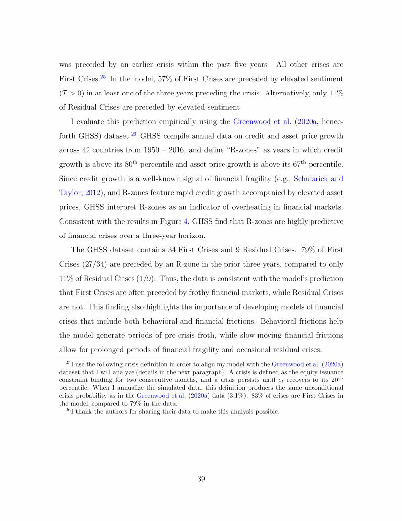
Figure 8 compares the estimated autocorrelation of the dividend-price ratio and
the investment-output ratio (blue) to the corresponding autocorrelation in the DEE
(red) and the REE (dashed black). The DEE is broadly consistent with the data,
particularly for longer horizons. This suggests that the long-run reversals produced
by the feedback from behavioral frictions to financial frictions improve the model’s
empirical fit. For robustness, Appendix Figure 10 plots these autocorrelations using
24These ratios are used because they are cointegrated. This helps to circumvent issues such asunit roots in investment and dividends. The concept of dividend-price cointegration is standard infinancial economics. For the investment-output ratio, see Cochrane (1994). Post-WWII data is usedto account for structural changes to the finance system (Schularick and Taylor, 2012).
37
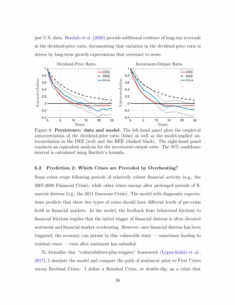
just U.S. data. Bordalo et al. (2020) provide additional evidence of long-run reversals
in the dividend-price ratio, documenting that variation in the dividend-price ratio is
driven by long-term growth expectations that overreact to news.
Dividend-Price Ratio Investment-Output Ratio
Figure 8: Persistence: data and model. The left-hand panel plots the empiricalautocorrelation of the dividend-price ratio (blue) as well as the model-implied au-tocorrelation in the DEE (red) and the REE (dashed black). The right-hand panelconducts an equivalent analysis for the investment-output ratio. The 95% confidenceinterval is calculated using Bartlett’s formula.
6.2 Prediction 2: Which Crises are Preceded by Overheating?
Some crises erupt following periods of relatively robust financial activity (e.g., the
2007-2008 Financial Crisis), while other crises emerge after prolonged periods of fi-
nancial distress (e.g., the 2011 Eurozone Crisis). The model with diagnostic expecta-
tions predicts that these two types of crises should have different levels of pre-crisis
froth in financial markets. In the model, the feedback from behavioral frictions to
financial frictions implies that the initial trigger of financial distress is often elevated
sentiment and financial market overheating. However, once financial distress has been
triggered, the economy can persist in this vulnerable state — sometimes leading to
residual crises — even after sentiment has subsided.
To formalize this “vulnerabilities-plus-triggers” framework (Lopez-Salido et al.,
2017), I simulate the model and compare the path of sentiment prior to First Crises
versus Residual Crises. I define a Residual Crisis, or double-dip, as a crisis that
38
was preceded by an earlier crisis within the past five years. All other crises are
First Crises.25 In the model, 57% of First Crises are preceded by elevated sentiment
(I > 0) in at least one of the three years preceding the crisis. Alternatively, only 11%
of Residual Crises are preceded by elevated sentiment.
I evaluate this prediction empirically using the Greenwood et al. (2020a, hence-
forth GHSS) dataset.26 GHSS compile annual data on credit and asset price growth
across 42 countries from 1950 – 2016, and define “R-zones” as years in which credit
growth is above its 80th percentile and asset price growth is above its 67th percentile.
Since credit growth is a well-known signal of financial fragility (e.g., Schularick and
Taylor, 2012), and R-zones feature rapid credit growth accompanied by elevated asset
prices, GHSS interpret R-zones as an indicator of overheating in financial markets.
Consistent with the results in Figure 4, GHSS find that R-zones are highly predictive
of financial crises over a three-year horizon.
The GHSS dataset contains 34 First Crises and 9 Residual Crises. 79% of First
Crises (27/34) are preceded by an R-zone in the prior three years, compared to only
11% of Residual Crises (1/9). Thus, the data is consistent with the model’s prediction
that First Crises are often preceded by frothy financial markets, while Residual Crises
are not. This finding also highlights the importance of developing models of financial
crises that include both behavioral and financial frictions. Behavioral frictions help
the model generate periods of pre-crisis froth, while slow-moving financial frictions
allow for prolonged periods of financial fragility and occasional residual crises.
25I use the following crisis definition in order to align my model with the Greenwood et al. (2020a)dataset that I will analyze (details in the next paragraph). A crisis is defined as the equity issuanceconstraint binding for two consecutive months, and a crisis persists until et recovers to its 20th
percentile. When I annualize the simulated data, this definition produces the same unconditionalcrisis probability as in the Greenwood et al. (2020a) data (3.1%). 83% of crises are First Crises inthe model, compared to 79% in the data.
26I thank the authors for sharing their data to make this analysis possible.
39
6.3 Prediction 3: Elevated Sentiment and the 2007-2008 Financial Crisis
This section applies the model to the 2007-2008 Financial Crisis in order to evaluate
the channels through which sentiment influenced the evolution of the crisis.
Measuring Sentiment in the Data. An open question in the diagnostic expec-
tations literature is how to measure sentiment in the data. Proposition 2 provides
a simple method. Sentiment can be constructed using forecast errors of economic
growth.
Proposition 2. Let σdZt = dYtYt− Et dYtYt = −θItdt+σdZt denote the economic growth
forecast error at time t. Sentiment It can be rewritten in terms of forecast errors as
follows:
It =
∫ t
0
e(−κ+θ)(t−s)σdZs. (24)
Proof. See Appendix B.5.
A feature of equation (24) is that it does not require parametric assumptions
about the data generating process for the economy. Given a calibration of κ and θ,
all that equation (24) requires is forecast errors of output growth.
Figure 9 uses the Survey of Professional Forecasters (SPF) to calculate sentiment
from 1970 through 2018.27 To initialize the calculation, I assume that sentiment equals
zero in January 1970. Since SPF forecasts are collected at a quarterly frequency,
Figure 9 is calculated using a discrete-time analogue of equation (24). Full details are
provided in Appendix A.2.
Sentiment in Figure 9 captures what Kindleberger (1978) refers to as “displace-
ment”: financial crises are preceded by large positive shocks to economic fundamen-
tals.28 Sentiment builds rapidly during the 1990s economic boom. Though sentiment
27Expectations data from macroeconomic professionals is most consistent with the model, sincesophisticated intermediaries are responsible for pricing risky assets.
28Cao and L’Huillier (2018) observe that the three deepest recessions in developed countries alloccurred roughly 10 years after periods of rapid technological innovation.
40
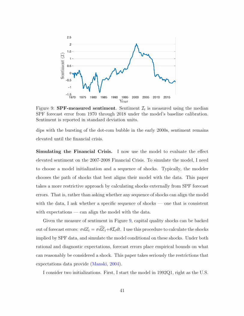
Figure 9: SPF-measured sentiment. Sentiment It is measured using the medianSPF forecast error from 1970 through 2018 under the model’s baseline calibration.Sentiment is reported in standard deviation units.
dips with the bursting of the dot-com bubble in the early 2000s, sentiment remains
elevated until the financial crisis.
Simulating the Financial Crisis. I now use the model to evaluate the effect
elevated sentiment on the 2007-2008 Financial Crisis. To simulate the model, I need
to choose a model initialization and a sequence of shocks. Typically, the modeler
chooses the path of shocks that best aligns their model with the data. This paper
takes a more restrictive approach by calculating shocks externally from SPF forecast
errors. That is, rather than asking whether any sequence of shocks can align the model
with the data, I ask whether a specific sequence of shocks — one that is consistent
with expectations — can align the model with the data.
Given the measure of sentiment in Figure 9, capital quality shocks can be backed
out of forecast errors: σdZt = σdZt+θItdt. I use this procedure to calculate the shocks
implied by SPF data, and simulate the model conditional on these shocks. Under both
rational and diagnostic expectations, forecast errors place empirical bounds on what
can reasonably be considered a shock. This paper takes seriously the restrictions that
expectations data provide (Manski, 2004).
I consider two initializations. First, I start the model in 1992Q1, right as the U.S.
41
is emerging from a minor financial crisis.29 This initialization takes a long-run view
of the 2007-2008 Financial Crisis in order to understand the full effect of the 1990s
IT boom on the subsequent crisis. I initialize et at the boundary of the crisis region,
and It at the 1992Q1 value shown in Figure 9.
The long-run simulation from 1992 through 2018 is shown in Appendix Figure 5.
I compare the simulation to the data using the He et al. (2017) Intermediary Capital
Ratio, which serves as an empirical counterpart to capital capacity et. In this single-
shock model with shocks taken externally from SPF forecast errors, the correlation
between et and the Intermediary Capital Ratio is 0.78 in the DEE. Using the same set
of shocks, the correlation is only 0.41 in the REE. The difference in fit is driven by a
divergence between the DEE and the REE over the mid-2000s. In the DEE, elevated
sentiment from the 1990s boom leads to an erosion of capital capacity prior to 2007.
In the REE, the financial sector remains well-capitalized throughout the mid-2000s
(further details below).
Though diagnostic expectations allow the model to qualitatively replicate the em-
pirical profile of intermediary capitalization over this boom-bust period, this long-run
simulation points to a failure of the model. Using the shocks implied by SPF forecast
errors, the model cannot jointly fit the 1990s boom and the 2007-2008 Financial Cri-
sis. Though the DEE comes much closer than the REE, neither produces a financial
crisis in 2008: the sequence of positive shocks realized throughout the 1990s places
the financial sector too far above the crisis region for the negative shocks in 2007 and
2008 to generate a full-blown crisis.
This formal failure is not surprising. This test tasks the model with replicating
almost 30 years of macro-financial dynamics using a single shock process that is cal-
culated externally from SPF forecast errors. The dot-com crash triggered significant
turmoil in financial markets, but had relatively muted effects on the real economy.
Because the model features only one shock process, it cannot capture such differenti-
29See, for example, the crisis dating of Romer and Romer (2017) and Baron et al. (2020).
42
ation between financial markets and the real economy.30
In light of this failure, the second initialization starts at the trough of the tech
bubble’s collapse in 2002Q4. et is initialized to edistress (the 33rd percentile of et) in
order to capture the tightness of financial conditions at that time. The initialization
of et can be thought of as applying a single MIT shock to the financial sector in
order to capture the differential effect of the dot-com crash on financial markets. Itis initialized to the 2002Q4 value shown in Figure 9. Proceeding from this starting
point, again using the shocks calculated from the SPF, the results of the simulation
are plotted in Figure 10.
The top panel of Figure 10 shows the time path of capital capacity et in the DEE
(red, left axis) and the REE (dashed black, left axis). The gray area marks the crisis
region. For comparison, the blue curve (right axis) plots the Intermediary Capital
Ratio of He et al. (2017).
The key result from the simulation is that only the DEE produces a financial
crisis. This is not to say that it is impossible to generate a financial crisis in the REE,
but, rather, that doing so requires large negative shocks that are inconsistent with
empirical forecast errors.31 This highlights the amplification of financial fragility that
elevated sentiment can produce. In particular, the divergence of the et profiles from
2002 through 2008 shows how a sentiment-driven crisis evolves. Realized shocks are
mild over this period, so capital capacity in the REE recovers quickly from initial
distress. In the DEE, elevated sentiment implies that balance-sheet vulnerability
persists throughout the mid-2000s. This leaves intermediaries exposed to the negative
shocks that hit in 2008.
The middle panel evaluates the model’s ability to replicate patterns in risk premia.
30Though sacrificing parsimony, this suggests that the model’s fit can be improved with additionalshocks that differentially affect the financial sector and the real economy.
31He and Krishnamurthy (2019) reach a similar conclusion when applying their rational modelto the 2007-2008 Financial Crisis, and show that “hidden leverage” is important for understandingthe crisis. The goal of my model with diagnostic expectations is to complement and build on thisconclusion by microfounding non-rational beliefs and systematizing the channels through whichsentiment can endogenously trigger neglected risk in financial markets.
43
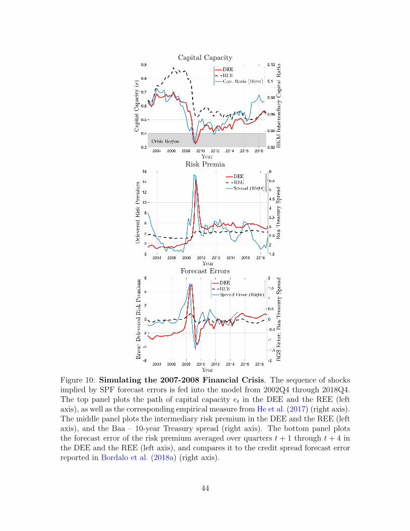
Capital Capacity
Risk Premia
Forecast Errors
Figure 10: Simulating the 2007-2008 Financial Crisis. The sequence of shocksimplied by SPF forecast errors is fed into the model from 2002Q4 through 2018Q4.The top panel plots the path of capital capacity et in the DEE and the REE (leftaxis), as well as the corresponding empirical measure from He et al. (2017) (right axis).The middle panel plots the intermediary risk premium in the DEE and the REE (leftaxis), and the Baa – 10-year Treasury spread (right axis). The bottom panel plotsthe forecast error of the risk premium averaged over quarters t + 1 through t + 4 inthe DEE and the REE (left axis), and compares it to the credit spread forecast errorreported in Bordalo et al. (2018a) (right axis).
44
This panel plots the realized risk premium earned by intermediaries in the DEE (red,
left axis) and the REE (dashed black, left axis), as well as the Baa – 10-year Treasury
spread for comparison (blue, right axis). The DEE broadly reproduces the path of risk
premia around the crisis. Pre-crisis risk premia are low. This is consistent with the
narrow spreads observed prior to the crisis, which many argue were due to neglected
risk (e.g., Gennaioli and Shleifer, 2018). Once the crisis hits, risk premia spike.
Because the crisis de-biases expectations, post-crisis risk premia remain persistently
higher than pre-crisis risk premia. Alternatively, because the REE never enters a
crisis, it exhibits almost no variation in risk premia over the simulated period.
The bottom panel assesses how these reversals in risk premia are reflected in
beliefs. The red and dashed black curves plot forecast errors in the DEE and the REE,
respectively (left axis). Specifically, this figure plots intermediary forecast errors of
the delevered risk premium averaged over quarters t+1 through t+4. The blue curve
(right axis) plots the corresponding forecast error of the Baa – Treasury spread, as
reported in Bordalo et al. (2018a).32 As in the data, the DEE generates large positive
forecast errors heading into the crisis, and large negative forecast errors exiting the
crisis. The REE produces only modest forecast errors, because risk premia exhibit
little variation away from the crisis region in the REE.
7 Conclusion
This paper develops a general equilibrium macroeconomic model that combines fric-
tions in financial intermediation with diagnostic expectations. The model examines
how the interplay of behavioral and financial frictions drives macro-financial dynam-
ics. When the financial sector is distressed, elevated sentiment amplifies systemic
risk and sets the stage for financial crises. For the broader macroeconomy, the con-
flicting short-run and long-run effect of diagnostic expectations generates endogenous
boom-bust patterns in investment and output growth. Even with this business cycle
32This data was kindly provided by the authors.
45
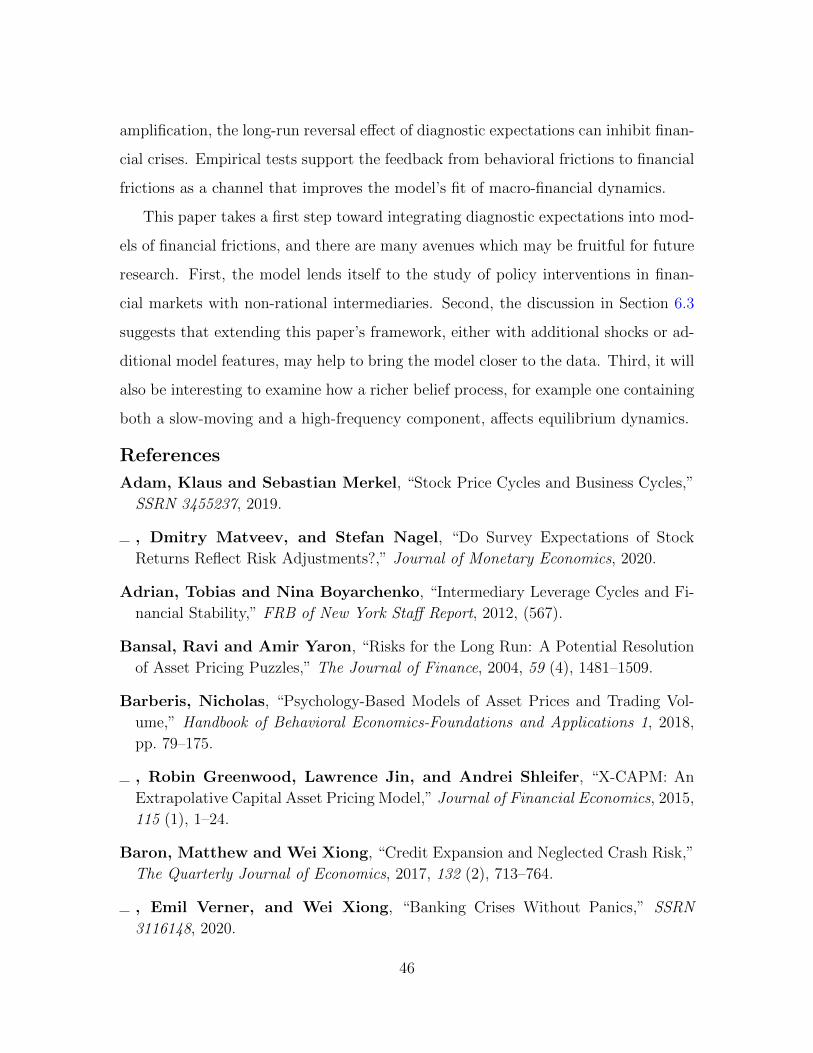
amplification, the long-run reversal effect of diagnostic expectations can inhibit finan-
cial crises. Empirical tests support the feedback from behavioral frictions to financial
frictions as a channel that improves the model’s fit of macro-financial dynamics.
This paper takes a first step toward integrating diagnostic expectations into mod-
els of financial frictions, and there are many avenues which may be fruitful for future
research. First, the model lends itself to the study of policy interventions in finan-
cial markets with non-rational intermediaries. Second, the discussion in Section 6.3
suggests that extending this paper’s framework, either with additional shocks or ad-
ditional model features, may help to bring the model closer to the data. Third, it will
also be interesting to examine how a richer belief process, for example one containing
both a slow-moving and a high-frequency component, affects equilibrium dynamics.
References
Adam, Klaus and Sebastian Merkel, “Stock Price Cycles and Business Cycles,”
SSRN 3455237, 2019.
, Dmitry Matveev, and Stefan Nagel, “Do Survey Expectations of Stock
Returns Reflect Risk Adjustments?,” Journal of Monetary Economics, 2020.
Adrian, Tobias and Nina Boyarchenko, “Intermediary Leverage Cycles and Fi-
nancial Stability,” FRB of New York Staff Report, 2012, (567).
Bansal, Ravi and Amir Yaron, “Risks for the Long Run: A Potential Resolution
of Asset Pricing Puzzles,” The Journal of Finance, 2004, 59 (4), 1481–1509.
Barberis, Nicholas, “Psychology-Based Models of Asset Prices and Trading Vol-
ume,” Handbook of Behavioral Economics-Foundations and Applications 1, 2018,
pp. 79–175.
, Robin Greenwood, Lawrence Jin, and Andrei Shleifer, “X-CAPM: An
Extrapolative Capital Asset Pricing Model,” Journal of Financial Economics, 2015,
115 (1), 1–24.
Baron, Matthew and Wei Xiong, “Credit Expansion and Neglected Crash Risk,”
The Quarterly Journal of Economics, 2017, 132 (2), 713–764.
, Emil Verner, and Wei Xiong, “Banking Crises Without Panics,” SSRN
3116148, 2020.
46
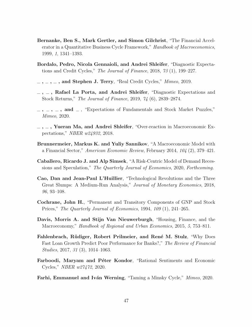
Bernanke, Ben S., Mark Gertler, and Simon Gilchrist, “The Financial Accel-
erator in a Quantitative Business Cycle Framework,” Handbook of Macroeconomics,
1999, 1, 1341–1393.
Bordalo, Pedro, Nicola Gennaioli, and Andrei Shleifer, “Diagnostic Expecta-
tions and Credit Cycles,” The Journal of Finance, 2018, 73 (1), 199–227.
, , , and Stephen J. Terry, “Real Credit Cycles,” Mimeo, 2019.
, , Rafael La Porta, and Andrei Shleifer, “Diagnostic Expectations and
Stock Returns,” The Journal of Finance, 2019, 74 (6), 2839–2874.
, , , and , “Expectations of Fundamentals and Stock Market Puzzles,”
Mimeo, 2020.
, , Yueran Ma, and Andrei Shleifer, “Over-reaction in Macroeconomic Ex-
pectations,” NBER w24932, 2018.
Brunnermeier, Markus K. and Yuliy Sannikov, “A Macroeconomic Model with
a Financial Sector,” American Economic Review, February 2014, 104 (2), 379–421.
Caballero, Ricardo J. and Alp Simsek, “A Risk-Centric Model of Demand Reces-
sions and Speculation,” The Quarterly Journal of Economics, 2020, Forthcoming.
Cao, Dan and Jean-Paul L’Huillier, “Technological Revolutions and the Three
Great Slumps: A Medium-Run Analysis,” Journal of Monetary Economics, 2018,
96, 93–108.
Cochrane, John H., “Permanent and Transitory Components of GNP and Stock
Prices,” The Quarterly Journal of Economics, 1994, 109 (1), 241–265.
Davis, Morris A. and Stijn Van Nieuwerburgh, “Housing, Finance, and the
Macroeconomy,” Handbook of Regional and Urban Economics, 2015, 5, 753–811.
Fahlenbrach, Rudiger, Robert Prilmeier, and Rene M. Stulz, “Why Does
Fast Loan Growth Predict Poor Performance for Banks?,” The Review of Financial
Studies, 2017, 31 (3), 1014–1063.
Farboodi, Maryam and Peter Kondor, “Rational Sentiments and Economic
Cycles,” NBER w27472, 2020.
Farhi, Emmanuel and Ivan Werning, “Taming a Minsky Cycle,” Mimeo, 2020.
47
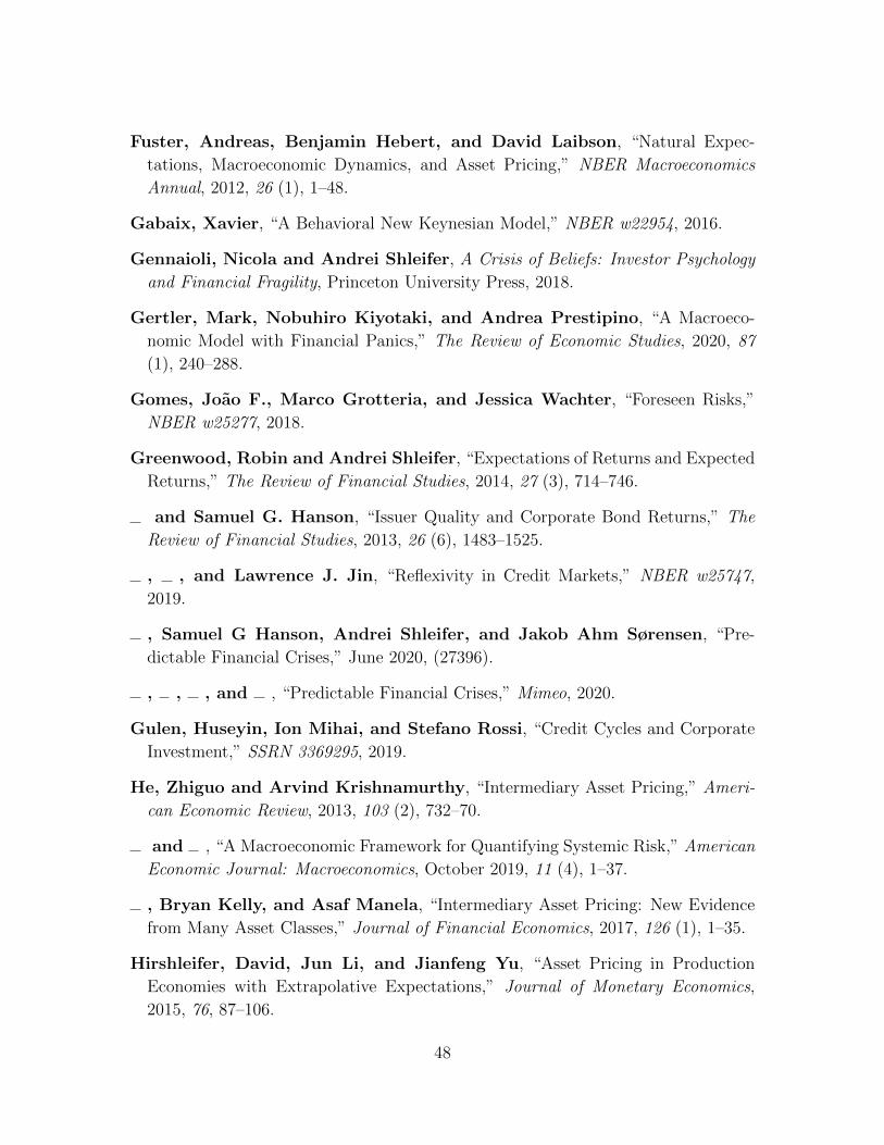
Fuster, Andreas, Benjamin Hebert, and David Laibson, “Natural Expec-
tations, Macroeconomic Dynamics, and Asset Pricing,” NBER Macroeconomics
Annual, 2012, 26 (1), 1–48.
Gabaix, Xavier, “A Behavioral New Keynesian Model,” NBER w22954, 2016.
Gennaioli, Nicola and Andrei Shleifer, A Crisis of Beliefs: Investor Psychology
and Financial Fragility, Princeton University Press, 2018.
Gertler, Mark, Nobuhiro Kiyotaki, and Andrea Prestipino, “A Macroeco-
nomic Model with Financial Panics,” The Review of Economic Studies, 2020, 87
(1), 240–288.
Gomes, Joao F., Marco Grotteria, and Jessica Wachter, “Foreseen Risks,”
NBER w25277, 2018.
Greenwood, Robin and Andrei Shleifer, “Expectations of Returns and Expected
Returns,” The Review of Financial Studies, 2014, 27 (3), 714–746.
and Samuel G. Hanson, “Issuer Quality and Corporate Bond Returns,” The
Review of Financial Studies, 2013, 26 (6), 1483–1525.
, , and Lawrence J. Jin, “Reflexivity in Credit Markets,” NBER w25747,
2019.
, Samuel G Hanson, Andrei Shleifer, and Jakob Ahm Sørensen, “Pre-
dictable Financial Crises,” June 2020, (27396).
, , , and , “Predictable Financial Crises,” Mimeo, 2020.
Gulen, Huseyin, Ion Mihai, and Stefano Rossi, “Credit Cycles and Corporate
Investment,” SSRN 3369295, 2019.
He, Zhiguo and Arvind Krishnamurthy, “Intermediary Asset Pricing,” Ameri-
can Economic Review, 2013, 103 (2), 732–70.
and , “A Macroeconomic Framework for Quantifying Systemic Risk,” American
Economic Journal: Macroeconomics, October 2019, 11 (4), 1–37.
, Bryan Kelly, and Asaf Manela, “Intermediary Asset Pricing: New Evidence
from Many Asset Classes,” Journal of Financial Economics, 2017, 126 (1), 1–35.
Hirshleifer, David, Jun Li, and Jianfeng Yu, “Asset Pricing in Production
Economies with Extrapolative Expectations,” Journal of Monetary Economics,
2015, 76, 87–106.
48
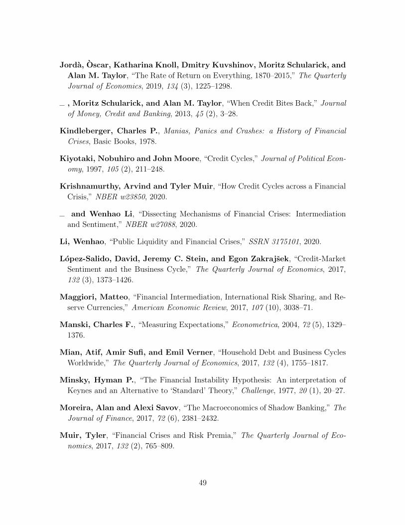
Jorda, Oscar, Katharina Knoll, Dmitry Kuvshinov, Moritz Schularick, and
Alan M. Taylor, “The Rate of Return on Everything, 1870–2015,” The Quarterly
Journal of Economics, 2019, 134 (3), 1225–1298.
, Moritz Schularick, and Alan M. Taylor, “When Credit Bites Back,” Journal
of Money, Credit and Banking, 2013, 45 (2), 3–28.
Kindleberger, Charles P., Manias, Panics and Crashes: a History of Financial
Crises, Basic Books, 1978.
Kiyotaki, Nobuhiro and John Moore, “Credit Cycles,” Journal of Political Econ-
omy, 1997, 105 (2), 211–248.
Krishnamurthy, Arvind and Tyler Muir, “How Credit Cycles across a Financial
Crisis,” NBER w23850, 2020.
and Wenhao Li, “Dissecting Mechanisms of Financial Crises: Intermediation
and Sentiment,” NBER w27088, 2020.
Li, Wenhao, “Public Liquidity and Financial Crises,” SSRN 3175101, 2020.
Lopez-Salido, David, Jeremy C. Stein, and Egon Zakrajsek, “Credit-Market
Sentiment and the Business Cycle,” The Quarterly Journal of Economics, 2017,
132 (3), 1373–1426.
Maggiori, Matteo, “Financial Intermediation, International Risk Sharing, and Re-
serve Currencies,” American Economic Review, 2017, 107 (10), 3038–71.
Manski, Charles F., “Measuring Expectations,” Econometrica, 2004, 72 (5), 1329–
1376.
Mian, Atif, Amir Sufi, and Emil Verner, “Household Debt and Business Cycles
Worldwide,” The Quarterly Journal of Economics, 2017, 132 (4), 1755–1817.
Minsky, Hyman P., “The Financial Instability Hypothesis: An interpretation of
Keynes and an Alternative to ‘Standard’ Theory,” Challenge, 1977, 20 (1), 20–27.
Moreira, Alan and Alexi Savov, “The Macroeconomics of Shadow Banking,” The
Journal of Finance, 2017, 72 (6), 2381–2432.
Muir, Tyler, “Financial Crises and Risk Premia,” The Quarterly Journal of Eco-
nomics, 2017, 132 (2), 765–809.
49
Nagel, Stefan and Zhengyang Xu, “Asset Pricing with Fading Memory,” NBER
w26255, 2019.
Pflueger, Carolin, Emil Siriwardane, and Adi Sunderam, “Financial Market
Risk Perceptions and the Macroeconomy,” NBER w24529, 2019.
Reinhart, Carmen M. and Kenneth S. Rogoff, “Recovery from Financial Crises:
Evidence from 100 Episodes,” American Economic Review, 2014, 104 (5), 50–55.
Romer, Christina D. and David H. Romer, “New Evidence on the Aftermath
of Financial Crises in Advanced Countries,” American Economic Review, 2017, 107
(10), 3072–3118.
Schularick, Moritz and Alan M. Taylor, “Credit Booms Gone Bust: Monetary
Policy, Leverage Cycles, and Financial Crises, 1870-2008,” American Economic
Review, 2012, 102 (2), 1029–61.
Tella, Sebastian Di, “Uncertainty Shocks and Balance Sheet Recessions,” Journal
of Political Economy, 2017, 125 (6), 2038–2081.
Tversky, Amos and Daniel Kahneman, “Extensional Versus Intuitive Reasoning:
The Conjunction Fallacy in Probability Judgment,” Psychological Review, 1983, 90
(4), 293.
Wachter, Jessica A. and Michael J. Kahana, “A Retrieved-Context Theory of
Financial Decisions,” SSRN 3333248, 2020.
Woodford, Michael, “Macroeconomic Analysis without the Rational Expectations
Hypothesis,” Annual Review of Economics, 2013, 5 (1), 303–346.
50