Embed Size (px)
Citation preview
NASA CR-152126 NASA-CR-152126) A MACH LINE-PANEL METHOD XN78-27087
FOR COMPUTING THE LINERIZED-SUPERZON-IC FLOW VER PLANAR WINGS (Boeing Commerciali Airplane CoS-eattle) 91 p HC A0-5MF 101 Unc~ds
CSC-L 011A G-302 25873
A Mach Line Panel Method for Computing the Linearized Supersonic Flow Over Planar Wings
FEdward Ehlers and Paul ERubbert
Boeing Commercial Airplane Company Seattle Washington
Prepared tor NASA Ames Research Center under Contract NAS 2-7729
4
RP 0 197
National Aeronautics and Space Administration
1978
httpsntrsnasagovsearchjspR=19780019144 2018-06-11T103010+0000Z
TECHNICAL REPORT STANDARD TITLE PAGE
1 Report No 2 Government Accession No 3 Recipients Catalog No NASA CR-152126
4 Title and Subtitle 5 Report Date A Mach Line Panel Method for Computing the May 1978 Linearized Supersonic Flow Over Planar Wings 6 Performing Organization Code
7 Authorls) 8 Performing Organization Report No F E Ehlers and P E Rubbert D6-46373
9 Performing Organization Name and Address 10 Work Unit No The Boeing Commercial Airplane Company P O Box 3707 11 Contract or Grant No
Seattle Washington 98124 NAS2-7729 13 Type of Report and Period Covered
12 Sponsoring Agency Name and Address National Aeronautics and Space Administration Contractor Report Washington DC
14 Sponsoring Agency Code
15 Supplementary Notes
16 Abstract
A method is described for solving the linearized supersonic flow over planar wings using panels bounded by two families of Mach lines Polynomial distributions of source and doublet strength lead to simple closed-forn solutions for the aerodynamic influence coefficients and a nearly triangular matrix yields rapid solutions for thesingularity parameters
The source method was found to be accurate and stable both for analysis and design boundary conditions Similar results were obtained with the doublet method for analysis boundary conditions on the portion of the wing downstream of the supersonic leading edge but instabilities in the solution occurred for the region containing a portion of the subsonic leading edge Research on the method was discontinued before this difficulty was resolved
17 Key Words 18 Distribution Statement
Linearized theory Unclassified-Unlimited Subsonic flow Panel methods Aerodynamics
19 Security Classif (of this report) 20 Security Classif (of this page) 21 No of Pages 22 Price
Unclassified Unclassified 86
Form DOT F 17007 (8-69)
FIGURES No Page 1 Mach Line Coordinates xy 63 2 Mach Line Paneling on Planar Wing at M= T 64 3 Analytic Continuation of the Doublet Distribution on the Wing Asociated
With an Interior Mach Line Panel at M = rT 65 4 Range of Interior Mach Line Panel and Analytic Continuation of Doublet -
Strength Outside of the Panel 66 5 Domain of Dependence of an Interior Panel With Illustration of Upstream
Characteristic Strips 67 6 Control Point Locations and Continuity Conditions for Doublet Mach Line
Paneling 68 7 Analytic Continuation of the Doublet Distribution on the Wing Associated
With a Mach Line Panel Adjacent to Supersonic Leading Edge at M =- r 69 8 Range of Integration for Supersonic Leading Edge Mach Line Panel Analytic
Continuation of Doublet Strength Outside of the Panel 70 9 Range of Integration for Subsonic Leading Edge Mach Line Panel and Analytic
Continuation of Doublet Strength Outside of the Panel 71 10 Pressure Distributions on Portion of the Wing Behind Supersonic Leading Edge 72 11 Pressure Distributions on Portion of the Wing Behind Subsonic Leading Edge
Along the Line y = 10603 73 12 Error in Downwash From Mach Line Doublet Panel Method Behind
Subsonic Leading Edge Along the Line y = 10603 74 13 Discontinuity in Pressure Coefficient Along Panel Edges of Mach Line
Doublet Panels in the Region Behind Subsonic Leading Edge 75 14 Pressure Distribution Along Line L Downstream of Special Mach Line With
Flat Plate Solution Superimposed on Doublet Panel Solution 76 15 Pressure Distribution Along Line L Downstream of Special Mach Line With
Flat Plate Solution Superimposed on Doublet Panel Solution 77 16 Pressure Distribution Along Line L Downstream of Special Mach Line With
Flat Plate Solution Superimposed on Doublet Panel Solution 78 17 Pressure Distribution Along Line L Downstream of Special Mach Line With
Flat Plate Solution Superimposed on Doublet Panel Solution 79 18 Control Point Locations and Continuity Conditions for Source Mach Line
Paneling 80 19 Comparison of Pressure Distribution From the Source Mach Line Panel Method
With the Exact Solution From Linearized Theory for Wing With Parabolic Are Profile 81
20 Comparison of Source Distribution With Wing Slopes 82 21 Comparison of Downwash From Supersonic Source Desigf Panel Method
With Actual Wing Slopes 83 22 Schematic Paneling on Wing Used to Test Mach Line Panel Methods 84 23 Region of Integration for Leading Edge Source Panel With the Zone of
Dependence Terminated by a Subsonic Leading Edge 85 24 Region of Integration for Interior Source Panel With the Zone of Dependence
Terminated by a Subsonic Leading Edge 86
v
CONTENTS Page
10 SUMMARY 1
20 INTRODUCTION 2
30 SYMBOLS AND ABBREVIATIONS 3
40 PLANAR MACH LINE DOUBLET PANEL METHOD WITH LINEARIZED BOUNDARY CONDITIONS 5 41 Theoretical Description of the Method 5 42 Discussion of Results From the Planar Mach Line Doublet Panel Method 10
50 PLANAR MACH LINE SOURCE PANEL METHOD WITH LINEARIZED BOUNDARY CONDITIONS 12 51 Theoretical Description of the Method 12 52 Discussion of Results From the Planar Mach Line Source Panel Method 13
60 CONCLUSION 15
APPENDIX A-DERIVATION OF BASIC FORMULAS FOR THE PLANAR MACH 16 LINE PANEL METHODS
Al Formulas for the Downwash from Supersonic Leading Edge
A3 Formulas for the Downwash from Subsonic Leading Edge
A5 The Doublet Distribution for Panels in Columns Behind the
A6 Doublet Distribution for Panels in Columns Behind the Subsonic
A7 Formulas for the Downwash in Columns Behind Supersonic
AS Formulas for the Downwash in Columns Behind Subsonic
Al1 Pressure Coefficient from the Supersonic Leading Edge Panels and
A13 Correction to the Pressure Coefficient from Supersonic Leading Edge Panels and from Interior Panels When the Subsonic Leading Edge
A14 Source Distribution for Panels in Columns Behind the Subsonic
Doublet Panels 16 A2 Formulas for the Downwash from Interior Doublet Panels 18
Doublet Panels 19 A4 Description of Panel and Parameter Numbering System 20
Supersonic Leading Edge (i lt ic ) 20
Leading Edge(i gti 23
Leading Edge lt ij 26
Leading Edge i gt ic) 27 A9 Matrix Equations for the Doublet Panel Method 29 A 10 Source Distribution for Columns Behind Supersonic Leading Edge 32
from the Interior Panels 35 A12 Pressure Coefficient from the Subsonic Leading Edge Panels 39
Panel of the Same Row is in the Zone of Dependence of the Control Point 40
Leading Edge 42
iii
CONTENTS (Concluded) Page
A15 Complete Pressure Coefficient from the Source Panels 45
APPENDIX B-INTEGRATION OF THE AERODYNAMIC INFLUENCE COEFFICIENTS FOR THE PLANAR MACH LINE PANELS 48
B3 Aerodynamic Influence Coefficients for Supersonic Leading Edge
B5 Aerodynamic Influence Coefficients for Subsonic Leading Edge
B6 Aerodynamic Influence Coefficients for Supersonic Leading Edge
B7 Aerodynamic Influence Coefficients for Rectangular Interior
B8 Aerodynamic Influence Coefficients for Subsonic Leading Edge
B9 Subsonic Leading Edge Correction to the Aerodynamic Influence Coefficients for Supersonic Leading Edge Source Panels and
BI Basic Integrals for Supersonic Leading Edge Panels 48 B2 Basic Integrals for Subsonic Leading Edge Panels 49
Doublet Panels 50 B4 Aerodynamic Influence Coefficients for Interior Doublet Panels 53
Doublet Panels 54
Source Panels 56
Source Panels 58
Source -Panels 59
Interior Source Panels 61
iv
A MACH LINE PANEL METHOD FOR COMPUTING THE LINEARIZED SUPERSONIC FLOW OVER PLANAR WINGS
FE Ehlers and PE Rubbert Boeing Commercial Airplane Company
10 SUMMARY
This report describes a study that was conducted in an attempt to develop advanced supershysonic panel methods in linearized supersonic flow This study centered around the use of panels bounded by the two families of Mach lines a feature which appeared at the outset to offer significant advantages Mach line paneling allows the accurate treatment of discontinuishyties in velocity and velocity gradient which occur along special Mach lines emanating from discontinuities in the wing planform The use of Mach line coordinates also leads to simple closed-form solutions for the aerodynamic influence coefficients By ordering the panels along characteristic or Mach line strips a nearly triangular matrix results for the simultaneous equations to be solved for the flow parameters The solution of the flow over the wing is therefore very rapid
Both doublet and source panel formulations were implemented and evaluated The doublet method was tested on a swept parabolic-cambered wing and the source method was tested on a swept wing with a symmetrical parabolic arc profile The source method was accurate and stable both for analysis boundary conditions in which wing slope is prescribed and for design boundary conditions in which surface pressure is prescribed and wing slope is computed Refining of the panel size improved the accuracy of the source method Similar results for analysis boundary conditions with the doublet method were obtained for the portion of the wing bounded on the downstream side by two Mach lines which intersect at an interior point and inclose only the supersonic leading edge However instabilities in the solution occurred for the region containing a portion of the subsonic leading edge
Research on the method was discontinued before the difficulty was resolved in favor of a method (ref 1) that appeared to offer more promise in terms of its adaptability to general nonplanar configurations This latter method subsequently underwent extensive developshyment and will be reported in a forthcoming NASA contract report
20 INTRODUCTION
Since wings in supersonic flow are usually thin and adequately described by linearized boundary conditions it is natural to represent the wing by doublet and source distributions on a plane In contract report NASA CR-2423 Mercer Weber and Lesferd (ref 2) proposed a method utilizing Mach line paneling on a plane with linearized boundary conditions and presented some preliminary analysis and classificatioi of panel forms which occur in a representative wing planform This report describes the continued investigation into this method
The approach appears to have several advantages
1 The Mach lines are well defined on the mean plane on which thickness and camber can be described by source and doublet distributions
2 As discontinuities in velocity and velocity gradient occur only across certain Mach lines denoted here as special Mach lines the discontinuities can be conveniently taken into account in the influence coefficients by appropriate paneling
3 With the two families of Mach lines as coordinates the region of integration for the source and doublet integrals on the plane is easily described and leads to simple closedshyform expressions for the influence coefficients
4 Solutions can be obtained extremely rapidly since the aerodynamic influence matrix can be placed in nearly triangular form by ordering the panels along characteristic strips on the wing planform
In this report both the source and the doublet Mach line panel methods are described in detail The source method for the thickness problem is very efficient and yields accurate results for both analysis and design type boundary conditions The doublet method for the camber problem was successful in regions directly behind the supersonic leading edges but exhibited instabilities in regions downstream of subsonic leading edges However because
-of-thsuccess of the subsonic panel method of Johnson and Rubbert (ref 1) and its greater applicability to a wide range of configurations and its apparent-extendability to supersonic flow the Mach line panel method described here was abandoned before the difficulty with the doublet method in the region behind subsonic leading edges could be resolved
The method discussed here is based on linearized supersonic flow theory The perturbation Velocity potential 0 is given by the Prandtl Glauert differential equation
(1- M2)0 oXo + 4yoy + ZtZo = 0
where M is the freestream Mach number and x0 y0 z0 are the Cartesian coordinates in the flow The freestream is in the x0 direction and the wing boundary conditions are applied on the z0 = 0 plane
2
30 SYMBOLS AND ABBREVIATIONS
abcd Coefficients in polynomial distribution of doublet strength
C(xy) Correction function for Mach line strips with a portion of the subsonic leading edge in zone of dependence (sec B9 of app B)
Cik Contribution to pressure coefficient from the kth panel in the ith column
Cp Pressure coefficient
fi(xy) Basic functions for integrals over leading edge panel i - 1 to 3 for supersonic leading edge panels and i = 4 to 6 for subsonic leading edge panels
G(ikxy) Polynomial used in doublet strength for the kth panel in the ith column
gi(xy) Downwash functions associated with the polynomial coefficients of doublet strength from supersonic leading edge panels i = 1234
T(xy) Pressure functions associated with source strength polynomial coefficients for supersonic leading edge j = 1234
hi(xy) Downwash functions associated with the polynomial coefficients of doublet strength from interior panels i = 1234
h(xy) Pressure function associated with the single coefficient of interior source panel
H0= i(x- )(y-n) Hyperbolic distance on the plane z = 0 in Mach line coordinates
i orj Column index
ic Column index for last column behind supersonic leading edge
k Index for panel number in any column
M Freestream Mach number
N(ikj) Doublet parameter numbers for the kth panel in the ith column j = 1234
Np(ik) = i(i-1)2 +k for i lt ic panel number for the kth panel in the ith column Np(ik) = [ic(ic+l) + (3ic - i + 2 ) (i - ic -1)] 2+k i gt ic
s1 Width of column in region behind supersonic leading edge
s2 Width of column in region behind subsonic leading edge
3
Si(xy) Downwash functions associated with the coefficients of the doublet strength in subsonic leading edge panels i = 1234
Sj (xy) Pressure function associated with the coefficients-of the source strength for subsonic leading edge panels j = 12
x0Y0Z0 Cartesian coordinates-x 0 aligned with the freestream
Xn Doublet parameters consisting of the polynomial coefficients of the double strength for all panels
xyz Mach line coordinate systemdefined-in equation (3)
xy Denote differentiation with respect to the designated variable when used as a subscript
xi x + i e s I panel coordinate for panels in the ith row from y coordinate axis
yj = y -is jIlt ic panel-coordinate in jth column forj lt ic
yj = y - icS1 - ( - ic+ 1)s2 panel coordinate for jth column for j gt ic
w Downwash
61 Slope of supersonic leading edge defined by x + ely = 0
E2 Slope of subsonic leading edge defined by x shy e2Y = 0
p Doublet strength
Ailk Total doublet strength in kth panel of ith column equations (A27) and (A34)
a Source strength
0 ik Total source strength in kth panel of the ith column equation (A64)
Perturbation velocity potential
4
40 PLANAR MACH LINE DOUBLET PANEL METHOD WITH LINEARIZED BOUNDARY CONDITIONS
41 THEORETICAL DESCRIPTION OF THE METHOD
The camber of a three dimensional wing of small curvature can be simulated by a doublet distribution on a plane In supersonic linearized theory the perturbation velocity potbntial q induced by such a doublet distribution is given by the integral
0 z0) 1 b p() dtdt7(Y(0 aoSWoo V(xo-E) 2 --B2 (yo -f )2 -B2 zo 2 (1)
where Sw is the portion of the wing cut by the upstream Mach cone from the point x0YoZ0 and B = M2-1 The velocity potential is normalized to the freestream velocity and the coordinates xyz to the wing chord The doublet distribution Ais determined by satisfying the downwash boundary conditions on the plane z0 = 0
az o = fxo (xoYo) (2)
where fXo (xoyo) is the slope of the camber surface z0 = f(x0 y0 ) The Mach line panel method of solving the boundary value problem of equation (2) is facilitated by introducing Mach line coordinates defined by the transformation (see fig 1)
zo =z
x0 - By0 = 2BxM (3)
x0 + By0 = 2ByM
Since the Jacobian of the transformation in equation (3) is 2BM 2 the potential in equation (1) in the new variables takes the form
1 8 2rM z-J (x-)(y--M 2 z2 4
Sw
Under the transformation in equation (3) the differential equation for 0 becomes
Ozz - M2 Oxy = 0
Differentiating the potential with respect to z and using the fact that the integral as well as 4 itself satisfies the differential equation we can replace the second derivative with respect to z by the second derivative with respect to x and y With this change in derivatives the evaluation of 0z on the plane z = 0 may be found by settingz = 0 in the integrand without first performing the differentiation (ref 3) Thus we obtain
5
Ma2 22 ) dd (4)
Oz= 2 r axayJxya 2x pij
Where = Q(i) and y = y(x) are the equations of the leading edge
In this form the integration must be performed before differentiation because of the inverse square root singularity of the integrand This problem is eliminated by introducing the new variables of integration
which lead to
a2 A( x -2M ff 2 y -n2 ) d~d7 (6)0
0
where we have dropped theprimes for convenience Some simplification results from pershyforming the differentiation before integratiofi When equation (6) is substituted into the boundary condition in equation (2) with the quantity fXo (xoyo) accordingly transformed into the Mach line coordinates in equation (3) an integral equation for the doublet distribushytion i(xy) results
Once the doublet distribution on the plane has been solved the pressure on the wing can be evaluated From the relationship implicit in equation (1)
Qim +=-p2
the pressure coefficient on the upper side of the wing is
MCp =-20 =Xo-MB( + centy (7)
The pressure coefficient on the lower side of the wing has the same magnitude but opposite in sign
The numerical approach to solving the integral equation using the Mach line panel method is to divide the wing planform into small panels by a grid system of the two families of Mach lines with x and y being constant and then determine the doublet distribution on each panel by imposing the appropriate boundary conditions at certain discrete points on the planform A typical paneled wing with M =Qis shown in figure 2 The paneling is comprised of
6
parallelogram-shaped interior panels having edges bounded by two families of Mach lines and triangular panels adjacent to the leading hnd trailing edges The doublet distribution on each panel is approximated by a polynomial with sufficient boundary and continuity conditions to establish the coefficients of the polynomial The doublet strength must vanish along a leading and side edge and be continuous across panel edges The downwash at certain points on the panels computed by summing the integrals of the form of equation (6) over all panels in the region of dependence must-equal to the prescribed camber slope at these same points
It is necessary that the doublet distribution be continuous over the planform as such disshycontinuities at panel edges introduce free vortex lines For convenience of the discussion we shall draw the paneling and wing planform in the oblique Mach line coordinate xy system as if it were orthogonal (which is the case for a Mach number ofVr The interior panels are then rectangular
In supersonic flow a rectangular panel influences the flow field in the region within the downstream Mach cone which emanates from the upstream vertex of the panel With Mach line paneling the panel edges coincide with the boundaries of this region as seen in figure 3 Continuity of the doublet strength is assured by choosing a polynomial which vanishes on the lines x = constant and y = constant defining the two upstream boundaries of the panel In terms of local panel coordinates with the origin at the upstream vertex of the rectangular panel the doublet strength p must be proportional to xy for rectangular panels within the planform ie
P = xy P(xy)
where P(xy) is a polynomial If we further postulate that on the downstream panel edges that the doublet strength be quadratic this restricts p to the form
p = xy (a + bx + cy + dxy) - (8)
The relation for g is continued analytically along characteristic strips downstream of the panel trailing edges by its quadratic relation on the downstream boundaries x = Ax and y = Ay where Ax and Ay are the panel length and width respectively Hence the contribution to p in the two downstream characteristic strips containing the panel is quadraticin the Mach line variable running normal to the edge (see fig 3) In the remaining portion of the domain of influence bounded by the two characteristics or Mach lines from the downstream vertex the doublet strength p is constant as indicated in figure 3 The range of integration for control points in the four distinct regions of influence of the panel is illustrated in figure4 with the corresshyponding functional relations for the doublet strength described in equation (8)
The complete doublet distribution on a given interior panel consists of the function in equation (8) associated with that panel plus contributions from
1 The quadratic doublet strengths at the downstream edges of those panels in the two characteristic strips running upstream of the panel as shown in figure 5
7
2 The constant doublet strengths at the downstream corners of those panels within the region between the two upstream running characteristic strips
Equation (8) for the doublet strength has four free parameters which can be determined as follows
Continuity of the normal derivative (in which Mach line variables) is applied at the downshystream ends of the leading edges of the panel leaving two parameters to be determined by the downwash boundary conditions attwo control points on the panel see figure 6 Howshyever for an interior panel in which one of the leading edges is a special Mach line along which discontinuities in velocity or velocity gradient may occur the requirement of the continuity of the doublet gradient is-relaxed on this edge and is replaced by a downwash boundary condition The formulas for the downwash induced by a doublet distribution on interior panels are derived in section A2 of appendix A They are simple rational algebraic expresshysions
The treatment for a triangular panel adjacent to a supersonic leading edge is similar Since the doublet strength must vanish on the leading edge of the wing the doublet distribution must be of the form
p = (x + ely) (a + bx + cy + dxy) (9)
where x + ely = 0 defines the portion of the leading edge covered by the panel and the origin is on the upstream corner of the panel illustrated in figure 7 It is easily seen that p vanishes on the x and y Mach line boundaries of the zone of influence for the leading edge panel In the same manner as for the interior panels the value of doublet strength is continued along the two characteristic strips by the quadratic relations on its downstream boundaries In the region defined by the two x and y Mach lines from the downstream vertex the doublet strength p is constant The range of integration for control points in the four distinct regions of influence of the panel is illustrated in figure 8 The four free parameters in equation (9) are determined as follows
In order to ensure the continuity of the doublet gradient along all straight supersonic leading edges we require the polynomial (a + bx + cy + dxy) at the upstream corner to agree with the adjacent leading edge panel value as indicated in figure 6 The downwash boundary conditions at the upstream corner point the middle of the panel leading edge and near the downstream corner point furnish the-rest of the conditions to render the four parameters determinate The formulas for the downwash induced by a doublet distribution on supershysonic leading edge panels are derived in section Al of appendix A
For the subsonic leading edge panels we use a doublet distribution of the form given in equation (9) for the supersonic leading edge namely
u = (x - e2y) (a + bx + cy + dxy) (10)
8
Here the origin is at the upstream corner of the panel and x - e2y = 0 defines the panel leading edge The doublet distribution of equation (10) is continued along strips in the x direction by its value on the downstream boundary at x = e2 s2 and since 1 vanishes on the leading edge p also vanishes for y gt s2 (see fig 9) The range of integration for control points in the three distinct regions of influence of the panel is illustrated in figure 9 The four free parameters in equation (10)-are determined by imposing the edge conditions and the downwash condition With the choice of doublet distribution given in equation-(10) the condition of vanishing doublet strength on the leading edge is automatically satisfied The continuity of the doublet gradient across the downstream edge is enforced when determining the parameters for the interior panels The continuity of the doublet strength along the upstream panel edge determines two parameters (a and b) in equation (10) One relation is to satisfy the continuity of the normal gradient of the doublet strength on the downstream corner of the same edge leaving only a single parameter to be determined by the downwash condition at one control point see figure 6 In case the upstream Mach line edge is a special Mach line the continuityof the doublet normal gradient is relaxed and replaced by a downwash for the same reason described for the interior panels
The derivation of the downwash from the subsonic leading edge panel is presented in section A3 of appendix A and in section-B5 of appendix B and results are given by equations (A13) and (B 19) The calculated downwash on the subsonic leading edge has a logarithmic singularity as seen from the function f4 in equationi (BS) Since p is approximated by a polynomial the tangential velocities are finite on the subsonic leading edge whereas analytical solutions for subsonic leading edge wings contain an inverse square root singularity in the tangential velocity at the leading edge No wakes were included in the examples computed by the doublet Mach line panel since there was no subsonic trailing edge For all trailing edges continuity of t on the wing with the trailing vortex sheet must be maintained From equation (7) we see that for continuity of pressure icross the sheet the doublet distribution on the wake must be of the form
A= Pn(x-y)
where Pn is a polynomial From equation (9) the expression for A on the panel adjacent to on either a supersonic or subsonic trailing edge of the form
= x e3y
is a polynomial of the fourth degree in x or y Hence Pn must also be a quartic in its argument x-y and the coefficients must be chosen to make p continuous at the trailing edge For a subsonic trailing edge panel a downwash control point must be located on the trailing edge to satisfy the Kutta condition of smooth flow
As seen from equations (8) (9) and (10) for the doublet distribution on a panel there are four parameters to be determined by appropriate conditions on each panel For supersonic leading edge panels we require the polynomials
a + bx + cy + dxy
9
to agree with adjacent leading edge panelvalies at all corners This ensures continuity of the gradient along all straight supersonic leading edges and leaves three parameters to satisfy the downwash boundary conditions at three control points
For interior panels continuity of the normal derivative-(8bx or 8by) of the doubletstrength is applied at the downstream ends of the two leading edges of the panel leaving two parameters free to be determined by downwash boundary conditions at two control points on the panel However for interior panels in which one of the leading edges is a soecial Mach line along which discontinuities in velocity or velocity gradient may-occur the requireshyment of the continuity of the doublet gradient is relaxed on this edge and is replaced by a downwash control point (see fig 6)
For subsonic leading edge panels two relations are required to satisfy continuity of pt with the upstream Mach line edge One relation is used to satisfy continuity of the normal gradient of the doublet on the downstream corner of the upstream Mach line edge leaving only a single parameter to be determined by a downwash control point
The control point locations and continuity conditions are illustrated in figure 6 for the wing planform used to test the method Design type boundary conditions also are possible with the x0 component of the perturbation velocity prescribed at the control points instead of the wing camber slopes
42 DISCUSSION OF RESULTS FROM THE PLANAR MACH LINE DOUBLET PANEL METHOD
To test the method described in the foregoing discussion a cambered swept wing of zero thickness having a parabolic arc profile was chosen The camber is defined by the formula
z1 =2t(I-Cyl) (x1 -x 12 ) (11)
where the yl axis is along the leading edge and the x1 axis perpendicular to the yl axis A closed form exact solution of the linearized differential equation was derived to check against the panel method for the portion of the wing planform described in figure 6
For the region downstream of the supersonic leading edge and upstream of the special Macl line the panel method yields results in close agreement with the exact solution from linearized theory for C = 03 and a wing sweep of 30 at a Mach numberv-as shown in figure 10 The pressure distribution normalized to maximum camber was fairly insensitive to location of the control points in the panels For the supersonic leading edge triangular panel best results were obtained for the interior control point located at the downstream corner Increasing the panel density improved the pressure distribution
In the region behind the subsonic leading edge (or free edge aligned with the freestream) the predicted pressure distribution was poor Increasing the panel density only served to
increase the deviation from the closed form solution A typical pressure distribution along a line close to and parallel to the special Mach line emanating downstream from the corner is shown in figure 11 The difference between calculated downwash distribution and wing slope follows a similar oscillating behavior in figure 12 The zero downwash difference values occur at control points where the boundary conditions were applied
10
Continuity of the normal derivative of the doublet distribution at corners ensures the conshytinuity of the pressure at corners The pressure distribution on both sides of a row of panel edges as shown in figure 13 demonstrates that this condition was properly applied in the solution The greatest discontinuity in pressure appears at the middle of the panel edge
To test whether the difficulty stemmed from the corner where the subsonic and supersonic leading edges join the flat plate conical flow solution was added to the panel method to eliminate the singularity along the special Mach line The pressure distributions along Mach lines in the region behind the free edge are shown in figures 14 through 17 Considerable improvement resulted and the match -with the exact solution in first column of panels downshystream of the special Mach line is excellent Away from the corner the pressure distribution appears to oscillate about the exact solution From the form of the oscillations if would appear that they are induced by the triangular subsonic leading edge panels which for this case is a free edge
A few attempts were made to alleviate this difficulty An additional control point was added to the triangular leading edge by adding to the doublet distribution the term
P =cx [(yx) -e2(yx)2] (12)
which corresponds to a conical flow pressure distribution This failed to improve the pressure distribution
Adding control points in the panels downstream of the special Mach line and applying mean square solution techniques to the set of simultaneous solution had a small effect in smoothing the result However as the condition of the continuity of normal derivative at panel corners was relaxed the discontinuities of pressure along the panel edges become larger and also affect the solution in the region behind the supersonic leading edge
11
50 PLANAR MACH LINE SOURCE PANEL METHOD WITH LINEARIZED BOUNDARY CONDITIONS
51 THEORETICALDESCRIPTION-OF THE METHOD
To solve the thickness problem for a planar wing we use a source distribution over the wingplanform The velocity potential in terms of Mach line coordinates of equation (3) may be written down by appropriately dropping the z derivative in the expression for the doublet potential Thus we have
a (71) -L ff d dn
2-- Sw (x- )(y -7)-M z 4 (13)
This integralhas the property that
oz Iz =+0= plusmna (x y)2 = (dzldxo) Z= plusmnO
where dzdx0 is the wing thickness slope Dropping the factor 2 relates a directly to the wing upper slope The pressure on the wing is given by
Cp = - 2 Ox = - M (o + y)BIz =0 (14)
Since we are interested in the flow properties on the wing it is convenient to set z = 0 in equation (13) before differentiating with respect to x and y Thus on the plane z = 0
_ y(x) j(n) aQt71) dtdn yY x N(x - _)y - 75
Vy --y(x) Vx -Q_(y-nq2 ) =__4 f f (x-t2 y-72) dn7M 0 0 (15)
where x = 2(y) or y y(x) describes the wing (or panel) leading edge
The source panel method follows essentially the same procedure as the doublet panel method and we will use the same wing planform paneling to illustrate the method (see fig 18) For supersonic leading edge panels a quadratic source distribution in the following form is used
u = a + bx + cy + dxy (16)
where the origin is at the upstream comer of the panel One parameter is fixed by requiring a to be continuous along the leading edge The other three parameters are determined from tangency conditions at three control points The source strength is continued outsidea the panel along characteristic strips by its linear values on the downstream panel edges in the same manner as described for the doublet strength
12
Continuity of source strength with interiorpanels is maintained by defining the source
strength on interior panels by a relation of the form
a = dxy (17)
where the origin of coordinates is at the upstream corner of the panel Since there is only one parameter d it is determined by a single downwash control point (or pressure)at the panel center The source strength of the interior panel is continued by its linear relation on its downstream boundaries in a manner similar to the doublet strength distribution
For subsonic leading edge panels the source distribution is given by
o = cy + dxy (18)
where the two parameters are determined by imposing the tangency condition at two distinct points shown in figure 18 Unlike the doublet panels the value of a on the upshystream characteristic strip is continued into the subsonic edge panel since a does not necesshysarily vanish on wing edges either subsonic or supersonic
For the planform in figure 18 the relatidn for a on a given panel is derived in appendix A and appendix B along with formulas for the pressure coefficient The same basic functions appear in the pressure coefficient for the source as in the formulas for the doublet downwash
Either analysis (ie upper surface slope) boundary conditions or design (ie pressure coefficient) boundary conditions may be applied The location of control points is shown in figure 18 Since Cp has a logarithmic singularity on the subsonic leading edge the control point must be moved off the edge of the subsonic leading edge panel for design boundary conditions
52 DISCUSSION OF RESULTS FROM THE PLANAR MACH LINE SOURCE PANEL METHOD
To test the source panel method a wing with a symmetric parabolic are profile was chosen which has the same spanwise and chordwise variation in slope for the upper surface as the cambered zero thickness wing used to test the doublet method (eq (11)) The angle of sweep is 300 and the freestream Mach number issect The subsonic leading edge angle was selected to make an isosceles triangle with the downstream Mach line boundary as shown in figure 19 The exact linearized solution is easily obtained in closed form and was used as a comparison with the panel method results
Figure 19 shows a plot of the pressure distribution from the panel method using six panels The agreement with the exact solution is very close Althoughthe results of the panel method is indicated by circled points the distribution is continuous in the whole region Figure 20 shows a comparison of source distribution from the panel method with the wing slopes along the lines shown in the planform in the figure This indicates that the boundary conditions are appropriately satisfied
13
The design mode was also tested using the same wing In this case the applied boundary condition was the theoretical pressure distribution from the exact linearized solution and the coefficients of the source distribution were solved for The resulting source distribution is seenito-be-in close-agreement-with-the-wing-slops asindicated in figure 21
14
60 CONCLUSION
The source panel method yielded very accurate results when either analysis (downwash) or design (pressure) boundary conditions were applied The doublet method gave accurate results for analysis boundary conditions on regions behind a supersonic leading edge Both methods were very stable and showed little sensitivity with variation in the location of control points on the panel Refining-the paneling improved the accuracy
However when theportion of the wing behind the subsonic leading edge was included in the solution the doublet method became unstable and sensitive to control point location Refinement of the paneling did not improve the accuracy but increased the oscillations in the panel solution and its departure from the exact linearized solution The difficulty appears to lie in an unsuitable treatment of triangular panels occurring along the subsonic leading edges
Research was discontinued on this method before the difficulty on the subsonic leading edge was resolved The success and stability of the subsonic method for nonplanar surfaces developed by Johnson and Rubbert (ref 1) suggested that it would also be suitable for supersonic flow Such an approach also has the advantage of producing methods for both subsonic and supersonic flow which are compatible with respect to paneling and control point location
15
APPENDIX A DERIVATION OF BASIC FORMULAS
FOR THE PLANAR MACH LINE PANEL METHODS
Al FORMULAS FOR THE DOWNWASH FROM SUPERSONIC LEADING EDGE DOUBLET PANELS
We shall now develop the basic formulas for the downwash from the panels located at three different regions on the planform using the doublet distributions presented in section 41 Consider first the downwash induced by a supersonic leading edge panel Since the doublet strength is continued on Mach line strips by its value on panel edges-the range of integration for points on and off the panel is-illustrated in-figure-8
For simplicity we shall consider cases b and d only The other cases can be easily obtained by dropping some of the terms Thus we have from equation (4) for case b when x lt 0 YgtSl
w_ 2 x~32 1 l ixle If xf 17 n)dd7H o + yf xJf Sl) ddiH o (Al)
and for case d when x gt 0 y gt s1
w=-- f d+ fQ(+ M07)dA di7 27r axay 0 H x
[(+ f s l dt+ f --- drj (A2)y 0 Ho x Ho
where Ho V(X )(y - )=
With the integrals in their present form the integration must be performed before the differentiation When the variables of integration are changed to
v= Vx -7 7= Ty-7 (A3)
the differentiation may be performed first The integral equation (Al) then takes the form for case b when x lt 0 y gt s1
16
w 2 M a2 ]yxY+ - x+e 1 (y-t 2)
Ir axay 1117 P (iX- )0t
Sl-NY - V 1 0
+ f ff x-t2 Xl )dtd 0 0
Performing the differentiation and noting that g vanishes on the leading edge ie m(- eIyy) = 0 leads to
- y Y(-7 Y-r1Y72dl2X ( y - 712 )
- l1
+ f f (A4)
for case b in which x lt 0 and y gt s1 Similarly equation (A2) becomes
W =--72)yr2)di2 y(-el(Y- x+e(y-12)
-X+e 1 (y-
+ x ( 2 72)damp (AS)
for case d in which x gt 0 y gt s
The cases a and c in figure 8 easily result from the preceding equations by setting y-s 1 =Owheneverylts 1
Evaluating the integrals using equation (9) for g leads to the downwash in the form
W = (Me-ir) [a gl(xy) + b g2 (xy) + cg3 (xy)+ d g4 (xy)] (A)
The functions gi are presented in section B3 of appendix B
17
A2 FORMULAS FOR THE DOWNWASH FROM INTERIOR DOUBLET PANELS
For the interior panel the regions of integration are depicted in figure-4 We-shall-consider the-case-y gt sI and x gt eIs 1 The downwash integral then becomes
w=M a2 f f p (477) d~d7Ho27r axy ISl elsi
+ S [f el4s I -6 - s d + 1 S f 0 djdii
+ fO fels] P(slq rd-(A7)
sd xd I
In terms of the variables in equation (A3) we obtain after performing the differentiation
w- 24 f5 (- 2y-q2) d077j (x (AS)
since p(0Sl)= A(elsl0)=my(0s) 0
The remaining cases a b and c in figure 4 follow by setting f --sI equal to zero for y lt s and v7 sj = 0 for x lt elS Substituting equation (8) for p yields the following relation for the downwash
W = (M 7r)[ahl (xy)+b h2 (xy)+ch 3 (xy)+ dh 4 (x (A9)Y)]
where the functions hiare derived in section B4 of appendix B
18
A3 FORMULAS-FOR THE DOWNWASH FROM SUBSONIC LEADING EDGE DOUBLET PANELS
For the subsonic leading edge panels we use a doublet distribution of the form of equation (10) ie
u= (x -e 2 y) (a + bx + cy + dxy) (A10)
where the origin is at the upstream corner of the panel The doublet distribution of equation (Al 0) is continued along strips in the x direction by its value on theboundary x = e2s2 and vanishes for y gt s The special cases for the regions of integration are illustrated in2figure 9 The most general case c yields the downwash formula
21xy s2 2 61 H 7)d + xf 2 4sHo1 )) d d (All)8irxay [ o
1c2 s2 Hd4di
In terms of the variables in equation (A3) these integrals become after differentiation
+ z (y 272) _72) dd 2 ) =y _ y e 2 (y-1
7I r (2zs
+ f J xe 7)x _7 ~i (A12)
The cases a and b are easily derived from equation (A12) by setting v7Y-s 2 equal to zero whenever y lt s2 and similarlyxx-e-s equal to zero for x lt e2 s2 Substituting equation (A10) for p in equation (A12) and integrating yields the following form for the downwash
W =(M 27r) [aSi (c y) + bS2 (x y) + cS3 (x y) +dS 4 (x y)] (A13)
where the Sj =1 to 4) functions are derived in section B5 of appendix B
19
A4 DESCRIPTION OF PANEL AND PARAMETER NUMBERING SYSTEM
To test the method we choose a wing planform consisting of a straight supersonic leading edge followed by a straightsubsonic leading edge and consider the-region-bounded--by the two-leading edges and a Ma6h line which intersects the two edges as shown in figure 22 The planform in figure 22 is divided into two regions by the special Mach line from the corner which in turn are dividedby the other family of Mach lines into rectangular and triangular panels The panel numbering follows the sequence as shown in figure 22 The ith column has i panels for i lt ic Summing the-previous panels we see that the panel number Np for the kth panel in the ith column is
Np(ik) = i(i - 1)2 + k_k = I to i (A14)
Since there are four parameters (abcd) associated with each panel the parameter numbers associated with the kth panel of the ith column is given by
N(ikj) = 2i(i - 1) + 4(k - 1) +j j = 1 to 4 (A15)
Since the doublet distribution in each panel is referred to the-origin of coordinates at the upstream corners of each panel we define panel variables xi yj by
xi= x+ielst i=12 (A16)
yj = y -is lt ic J=l1 2 (A17)
where s1 is the column width behind the supersonic leading edge
Forj gt iwe havec
Yj=y-icSl-G-ic+1)s2 (AI8)
where s2 is the width of the subsonic Mach line columns Since es 1 --e2 s2 the definition of xifor igt icremains the same
AS THE DOUBLET DISTRIBUTION FOR PANELS IN COLUMNS BEHIND-THE SUPERSONIC-LEADING EDGE (i-lt ic)
It is convenient to define the function
G(i k x y) = XN(i k1)+X XN (i k 2) +Y XN(i k3) +XYXN(i k4) (A19)
where the XN correspond to the parameters (abcd) in equations (8) through (10) and N(ikj) is defined in equation (Al 5)
20
Then the contribution to the doublet distribution from variables related to the kth panel in the ith column is for i lt ic
j=xi-k+l yi-1 G(i k Xik+1 Yi-1) (A20)
for i gt k gt 2 for interior panels and
1=(xi1 Y+e G(i 1 Xi-l Yil) (A21)Yi-1)
for supersonic leading edge panels
We shall now construct pi in the kth panel of the ith column for columns behind the supersonic leading edge The upstream panels in the same row as the kth panel of the ith column are
Np (i-j k-j) forj = 123 k-I (A22)
These panels contribute to the x variation in the form
k-2 Xik+1 G(i-k+l 1 Xi_k Sl) + j Xi-k+1s1 G(i-j k-j xi-k+l s) (A23)
j=l
Similarly the upstream panel numbers in the same column are
Np(ik -j) i = 123 k-1
and they contribute to the variation with y in the form
k-I 1 yI G(i 1 Y -1) els1 Yi G(ij elS Yi-1) (A24)+ 2
j=2
The corner values from the remaining upstream supersonic leading edge panels contribute a constant term of the form
k-1 els 1 G(i-+1lOs1 (A25)
j=2
Contribution to the constant from the interior panels upstream of the k - I row from panels numbered
Np(i-jk-j-1) i = 123 k-3
21
is
k-3 ll2 G0i-j k-l-j elS1Sl-
Contribution to the constant from upstream k - 2 row is
E-4 elSl 2 G(i-j k-2-j el S1Sl)
j=1
and the total contributions to the constant from all upstream interior panels are
k-3 k-2-n 2 I 1 - elS1
2 G(i-jk-n-j elS1s) (A26) n1 j=1
Combining-equations-(A-23) (A24) (A25) and (A26) with the panel function itself yields the following value of Mik for the kth panel-in the ith column
Pik= xp-k+l yi_l G(I k xj k+l Yi-) + xifk+ G(i-k+l 1 xi_ksl)
i X-2 Xik+1 G(i-i k-j xiSk+l sl) + elYy1 G(i 10Yil)
j=1 1 1 i~is~ik+ ~es X i)- ik+ ii11O
cSl yi-l)++Z OlS1+-1y-Gij o(i-+1 0 Sl) j=2 j=2
k-3 k-2--fl + 2 -- ls12G(i-jk-n-jelslsl) (A27) n1l j=1
22
Equation (A27) holdsfor k gt 2 if those summations ate dropped for the particular values of k in which the upper limits are less than the lower limits
A6 DOUBLET DISTRIBUTION FOR PANELS IN COLUMNS BEHIND THE SUBSONIC LEADING EDGE (i gt ic)
Let ic be the last column for which the leading edge is supersonic The total number of panels in the region to the left of th special Mach line is
ic(i c + 1)2
The number of panels for i gt ic in the ith column is
i - (i- i - 1) = 2i0 - i + 1c c
By summing the panels in the columns up to the ith column we find that the panel number for the kth panel in the ith column is
Np (ik) ic (ic + l) + (3ic-i + 2)( i-ic-I)] 2+k (A28)
The numbers corresponding to the parameters in the panel are
N(ikj) = 4Np(ik) - 4 + j j = 1234 (A29)
For the subsonic leading edge panel we have
Ail = (X2ic~i+l - 62 Yi-l ) G (i lX2ic7i+ 1 Yil ) (A30)
The doublet distribution cannot be made continuous by analytically continuing the distribution from the upstream panel downstream into the subsonic leading edge panel since p must vanish on the leading edge Thus p must be matched in the subsonic leading edge panel on the upstream edge by two relationsobtained by equating the-two coefficients of the x variable
Consider the kth panel in the ith column for i gt ic Then the panel numbers for the panels in the same row for i gt ic are
Np(i -j k +j) = 123 i - ic - 1
The remaining interior panels upstream of the special Mach line in the same row are
Np (ic+ 1 -jk+i-ic-j) forj = k1 2 3 4 k+i-ic -2
where Np(ik) = i(i-1)2 + k for i lt i
23
The supersonic leading edge panel in the same row as the kth panel in the ith row is
Np (2ic-i-k+ 21)
Contributions to the x variable alone in p for the kth panel ofthe ith column are given by
i-i -1
i- X2ici+2_ k S2 G (i-j k+j X2ic~i+2_k s2)
j=1
+ X2ii+2_k G(2iC-i-k+2 1 X2ici-k+l I) (A31)
Contributions to-the y-variable in M for the kth panel of the ith column are
k-2 - - e2 s2 Y iG0 k-J 62S2 Yi-1)
j=l1
-e 2 y i G(i 1- e2s2 Yi-1)
+ x2ic-i+2-k Yi-1 G(i k X2ici+2_k Yi-1) (A32)
Except for a constant lik is given by the sum of equations (A31) and (A32) For k = 2 this constant will be zero since til vanishes for yi-i = s2 and X2 i i- 1 = E282 a point on the leading edge
To make p continuous on the upstream edge of the first panel in the ith column we set k = 2 and replace i by i-I in equations (A3 1) and (A32)
=Combining the results for Yi-1 0 and equating to p defined by equation (A30) for Yi-1 = 0 we obtain
24
x2i1 _i+ l G(i 1 x2ic-i+l 0)
i-i--2
=X x2ici+1 s2 (i--i 2j x2 iei+l s2)j=0
i-it-1
+ X2ici+1 s 1 G(ic+l-j i-ic+l-j X2 ici+ s)
+ x2i i+1 G(2ie-i+l 1 x2ici Sl) (A33)
For the corner panel i = ic + 1 equation (A33) takes the form
xic G(ic+l 1 xj 0) = xic G(i c 1 xic 1 sl)
Using the relation x2i -i- = x2i -i -elsl combining coefficients of x2i -i and x2 2ic-i and setting the coefficients in equation (A33) equal to zero yields two relations which reduce the free parameters of the subsonic leading edge panel to two
To determine the constants resulting from the upstream panel comers for the columns i gt ic we note that the constants from the panel comers are incorporated into the subsonic leading edge by means of the continuity conditions in equation (A33) Hence for the kth panel in the ith column the contributions to the constant term in Pik occur only for the rows k - 1 to 2 Since the constant term itself does not affect the pressure distribution it will not be written down Accordingly the doublet distribution for i gt i takes the form
Pik = X2ici+2-k Yi- 1 G i k X2ici+2_k Yi-1
i-it-1 X2ic-i+2_-k s2 G i-j k-j x2i-i+2-k s2)
k~i-ic-2 + x2ici+2k Sl G(ic+l-j k+i-ic-j X2ici+2_k Sl)
j=1
+ X2ici+2_k G(2ic-i-k+2 1 X2ic i-k+l sl)
+ k-2E e2 s2 Yi-1 G(i k-j e2s2 Yi-1) j=1
-e2 Yi- 2 G(i 1 62s2 Yi-1) + constant (A34)
25
A7 FORMULAS FOR THE DOWNWASH IN COLUMNS BEHIND SUPERSONIC LEADING EDGE (i lt ic)
Let Wik be the contribution to the downwash bcpBz from -the-panelvaiables-in-the-kth panel-of-the-ith olufnn ForA ltic Wik is defined in equation (A6) for a supersonic leading edge panel (k = 1) in equation(A9) for-interior panels and by equation (A13) for subsonic leading edge panels For the total downwash at the point on the kth panel of the ith column we add the contributions from-all the panels upstream of the kth panel iff the ith column The contributions fr6rn the same row are
k-I S Wimk-m m=0
The contributions from the row above the kth panel are
k-2 2 Wi-mkm_1 m=0
and finally from all panels upstream ofthe kth panel of the ith column we have
k-1 k-n-1 W--_I S - Wi-m k-m-n
n-0 m=0
Since the downwash W is computed from a different formula for the supersonic leading edge panels than for the interior panels it is convenient to separate them thus we write
k-1 k-2 k-n-2 W = S Wi-m 1 + S1 Wi-mkmn (A35)
m=0 n=0- m=0
Substituting equations (A6) and (A9) into equation (A35) yields
4 k-I rWM VW I Z X(i-mlJ)gj (Xi-m-l Yi-m-1)
j=1 m=0
4 k-2 k-h-2 + T I I XN(i-m k-m-nj) hj (xik+n+yijm-l (A36)
j= n=0 m-0
where N(ikj) = 2i(i-1) + 4k +j - 4
26
A8 FORMULAS FOR THE DOWNWASH IN COLUMNS BEHIND SUBSONICLEADING EDGE (i gt ic)
We consider the downwash in the kth panel of the ith column where now i gt ic The panel number in the i column in the same row as the Np(ik) panel is
Np (iCi-ic+k-1 )
The contribution to W for all the panels in columns behind the supersonic leading edge is found from equation (A35) by setting i = ic and replacing k by i-ic + k-1 or
i-i0 +k-2 i-ic+k-3 i-i0+k-3-n
E Wi-m1 + z Z Wic-miic+k-l-m-n m 0 n=0 m=
The contributions of the downwash to the kth panel of the ith column from panels in the columns whose numbers are greater than ic and in the same or k row are
i-i--
F Wi-mk+mm=0
Similarly for the k-I row i-ic-1
m Wi-mk+m-1M7=0
and for all k-2 rows
k-2 i-ic-i O Wi-im k+m-nn 7-0 m=O0
The contributions from the suibsonic leadinig dge panels are
i-it-1
Wi-m1m=0
-and from the remaining interior panels
i-i-2 i-ic- 2-n E 2 - Wi-m-n-l2+m n=0 mO
27
The total downwash for-a point on the kth panel of the ith column for-i gt ic is finally
i-ic+k-2 -ic+k-3- i-ic+k-3-n W=c Wicml+ I - - mi-ic+k-l-m-n
m0 n7-0 m=O
i-ic- 1 k-2 W-i-1 +Z Wim + 1 1 -Wimk+mn
m=O nO m=O
i-it-2 - i-i--2-n
+ Sz Wi-m-n-i2+m (A37)n=0 m=0
For the supersonic leading edge we have
1Wic-ml MVIT
42 i7e-lj Xm_ Yc_ (A38) - j=l C
for the subsonicleading edge
rWi-mIMV shy
4 Z XN(i-milj) Sj (X2ic-i+m-lYi-n-) (A39)j=l
and for the interior panels in columns i gt ic
4 rWikMvf 62= 1 XN(ikj) hj (x2iei-k+2 Yi-r) (A40)
j=l
28
and for interior panels in columns i lt ic
4 lWikM rV = XN(ikj) hj (Xik+l Yil) (A41)
j=1
Note that for i lt ic
Yi-1 = y - (i - 1)s1
N(ikj) = 2i(i - 1) + 4(k - 1) +j (A42)
while for i gt ic
yi-1 = y -icSl - (ic -i +2) s2
N(ikj) = 2ic (ic + i) + 2(3ic - i + 2) (i - ic- 1)+ 4(k-1) +j (A43)
Continuity of downwash along the supersonic leading edge at panel corners requires continuity of the derivatives of p at panel comers For the point between the i and i+l columns this becomes
XN(i+I11) = XN(i11) - e1S )N(iI2) + S1 XN(i13) 7 elS1 2 XN(i14) (A44)
A9 MATRIX EQUATIONS FOR THE DOUBLET PANEL METHOD
At each panel both equations (A36) and (A37) forthe downwash reduce to an equation of the form
N Z AnXnW n=
where W is the local camber slope dzdx0 for the wing at a selected control point of the panel Four such equations are needed for each panel since there are four variables to be defined at each panel For subsonic leading panels two of these equations are-provided by the condition that g be continuous with the upstream panels by matching the coefficients of x and x2 in equation (A33) Another condition is the continuity of the normal gradient of p at a point on the upstream boundary of the panel This condition is relaxed for panels bordering a special Mach line where pressure or pressure gradients may be discontinuous The designation of downwash control points is indicated by dots and continuity of normal derivatives of p at panel boundaries is indicated by arrows in figure6 with the arrow heads lyingin the panels in which the conditions apply -These continuity conditions are prescribed at the supersonic leading edge panel corners at
x = 0 y =s
29
for interior panels at
x = 0 y =s
x= elsl Y= 0
and for subsonic leading edge panels at
x = el 1s = 62s2 y = 0
when expressed in local panelcoordinates Noting that
jand [ XQmG( a X2Ym)] =Ym G(Otf3 2xQYm) (A45)
x2 y3 GI~o 3X2 im)] = x2 G(a (3x2 2Ym)
the conditions that agax is continuous at Xi-k+l = el 1s and Yi- =-00 for the kth panel in the ith column is
ay ik Ik ay (A46)
From equation (A27) with he aid of equati6n (A45) equation (A46) becomes
s1 G ik-elSlo+G (i k-1 G (i l0 )10)+ Sl Z
i=2
k-2 +s 1 Z G (i-1 e2 sl 2s) (A47)
j=2
This leads to homogeneous e4uations df the form
N 1 An Xn=-O n-l
The other continuity condition
Ax =~ P I]4 (A48) ax ik-i3 00O elS 1 sI s1
30
with the aid of equations (A27) and (A45) leads to
s1 G (i k 0 s1) + XN(ik+l 1 1) - elSl XN(i-k+l 1 2)
- k-2 +sl1xN(i-k+i 1 3)-6lSl XN(i-k+l 1 4)] +s1 G (-j k-i0 si)
j=1
s 1 G(I k-i 2 el1 sl) + XN(ik+2 1 1) + elSl XN(i-k+21 2)
+ s [XN(ik+2 1 3) + eS XN(ik+2 14)]
k-3 +s E G i-j k-l-j 2 e1s s) (A49)
j=l
The case for which k = 2 must be treated separately Equation (A46) yields
5- [ 1 2 Y-il) + e1 Yi G01(i 0 Yijl)] elsX 0yi-
TYA (x 1-2 +el yI 2 ) 0(1-1 1 xp2 Y1 2 )] 0 5 1 A50 or
s1 G i 2s1 0) + G (1 0 0) = G(i- 1 0 2 s) (A5 1)
Similarly equation (A48) yields
X_[xi_l yi_ GO2 xi_ Yi-l ) + Xi-lG (ll xi_2Sl 1]]bull
TX[xi-i-l -I1)-lOxe G(i lxi Yl) 081 (A52)
or
s G (i-2 0Sl) + G (i-1 1-CISl Sl)
= Cisi [XN(i 1 2) +s XN( i 1 4)]+ G(i 1 0 s) (A53)
31
Continuity of pay on the upstream boundary of the subsonic leading edge panel of the ith column is found by setting k = 2 replacing iby i - 1 in equation (A34) and differentiating Thus with equation (A30) we have
TyX2i-i+1 yi-2 GOi-1 2 x2ioi-1 yi-2) -e2 Yi_3 G(i-1 1 62s2 Yi-2) ]e8s
--e2s2 s2
= [(x2ic-i+l - e2 Yt-1) G(i 1 X2ic7i+1 Yi4)a
or
s2 G(i-1 2 62s2 2 s2 ) -F 1 62 S2 2 s2)
- 2 [ XN(l13) +e2s2 XN(i 1 4)] - G(i 1 e2 s2 o)
Equations corresponding to equations (A47) and (A49)-for interior panels for i gt ic can be derived in a similar manner using equation (A34) for gik
A10 SOURCE DISTRIBUTION FOR COLUMNS BEHIND -SUPERSONIC LEADING EDGE
The source panel method follows essentially the same procedure as the doublet method and we use the same wing 15lanform to test the method For supersonic leading edge panels a quadratic source distribution in the following form is used
a a + bx + cy + dxy (A54)
where the origin is at the upstream corner of the panel Onie parameter is fixed by requiring a to be continuous along the leading edge For the supersonic leading edge panels denoted by subscripts I and 2and numbered l and 2 in figure 22 the continuity-conditioiis take the form
a2 =a1 - bel s1 + cs 1 - delsl 2 (A55)
for a leading edge of the form x + eIy= 0 Here sI is the panel width (y direction)
For interior panels we associate a single free parameter and modify the source distribution by
a = d xy (A56)
where the origin of x and y is at the upstream leading edge corner of the panel Since it vanishes on the leading edges it preserves continuity when a is continued downstream along Mach line strips by the value on the panel trailing edge in the same manner as the doublet panel method
32
To construct the value of the source at some kth interior panel in column i we consider the same wing as in the doublet method From figure 22 we define a in the leading edge panels as
a =a1 +b 1 +cly +d 1 xy
a2 a2 +b2 x + c2y 1 +d 2x y11
04 - a4 + b4 x2 + c4y2 + d4 x2y 2 (A57)
where xiy j has the same meaning as in the doublet paneling To preserve continuity the source distribution in panel 3 takes the form
o3 = aI ( x Sl + u2 (0Y1) - 2 (0 0) + d XlY1 (A58)
Since a2 = a1 - b els 1 + cs1 - d elsl 2 from equation (A55) we have
a l (x s l) -a 2 (0 0 ) = (b l +d s l) (x+elsl)
=(bj+d l s l ) x
from which
u3=(bl+dlsl) xl+a 2 +c 2 Yl+d 3 xlYl (A59)
and similarly
5= (b 2 + d2 S) x 2 + a4 + c4 Y2 + d5 x2 Y2 (A60)-
To find we writea6
a6 =a3 (xlsl) + 5 (elslY 2 )-a 5 (elsl 0) +d 6 xy 2 (A61)
or
0 6 =(b +d 1 sl ) x 1 +d 3 slx 1td 5 elS1 Y2 +d 6 +Y2l
+ a4 +c4 Y2 + (b 2 + d2s) elsl (A62)
We note that the supersonic leading edge panels are continued in the y characteristic strip in the form
(bl +dl s1 )X 1
and the constant term a only enters for the leading edge panel of the same column as the panel under consideration
33
The panel numbering system for the source panel method is identical to that used in the doublet panel method The panel number for i lt ic for the kth panel in the ith column is then given by
Np = i(i-1) 2 + k k=l12 i
For k-1 the leading edge panel ha four associated parameters while for all other k there is only one associated parameter The variable (or parameter) number in the kthpanel (k gt 1) is
N(ik) = i(i-1)2 + k + 3i -- i(i + 5)2 + k k gt I (A63)
For k = 1 the variable numbers are
N (ij)=i (i + 5 ) 2 +j-3 1=1234
The pattern in equation (A62) can be generalized and for the kth panel in the ith column we have
rik =(XN I (i-k+l2) + Sl XN1 (i-k+14)) Xi-k+l
k-2 + s1 _ XN(i-jk-j) Xl-k+l
k-2 + els1 T XN(ik-J) Yi-1
j= 1
+ XN1 (il) + XN (13)Yi-1 + XN(ik) xi-k+ Yi- 1
+ Y XNI(ij2 + s1 XN(i-j4) el s1j=l
k-3 k-2-n +e 1sl 2 Z Z XN(i-nk-m-n) (A64)
34
where N(ik) denotes the variable number for the kth panel defined for kgt 1 in equation (A63) and Nl(ij) denotes the variable numbers for the first panel of the ith column given by the equation following equation (A63)
All PRESSURE COEFFICIENT FROM THE SUPERSONIC LEADING EDGE PANELS AND FROM THE INTERIOR PANELS
The velocity potential resulting from a leading edge panel for points in the panel is seen from equation (15) to be
27rM f foxE~- dd 0 0
where x + eIy = 0 defines the leading edge
For points outside the panel x lt 0 y gt sj we have
4 fV+xl x+e I(yn 2 ) S-rM f (-2 ~ ~Tf2 GIxjxampyn2) dtdn
NF f u (xl-2s) d (A66) 0 0
For x gt 0 y lt Sl we obtain
4 [ x+ejl~2T
f Y a( X- 2Y-772)dtdn
1 f (A67)
0 0
35
Similarlyfor x gt 0 ygt s
- +-j (-i~~-rXir -- x 2l a2-dtdn
+ fV1 a (0y-n2)ddiY sl 0shy
+ o - (x t2 Sl) dyr7
0 0
Only equations (A66) and (A68) ieed be consideredsince the other two cases result from setting y - = 0 when y lt s andyx=0 when x lt 0 From equation (A66) the pressure coefficient becomes
j ~ 21 Xx2+ei)-z2
)=s (I (CP (oiY 1 +x+e )-d7 wt+rfth a ) is oy61 - 2 y a nce
+fy-Sl e1 2 Y7
+~ f x(X-t2Sl)dt
0 0
where the termf 0 (-elSlSl)d is dropped because of continuity of a at panel corners
0 2 Vx +elsl
36
Equation (A68) yields
l( - ~+el -1 2) )_l2)dL
Vx+e 1 (y-l 2 )
+ f f [ax(x_2y-72)+Uy(x-y2)]dd
+f f oy(Oy-2)ddq rY- Sl 0Il
+f ux(x-t2Sl) dd (A69) o axx-2sld n
where we have neglected the terms
1 1 i o-l 1 s ) d
2V )d 2-elS1 f -els1 si) d(OO and
which are cancelled because of the continuity of a at panel corners
Choosing a(xy) = a + bx + cy + dxy and integrating yields Cp in the form
Cp = (VeflirB) [aIg1 (xy) + b 92 (xy) + c 93 (xy) + d g4(xy)] (A70)
where the g functions are derived in section B6 of appendix B
For interior panels we use a source distribution of the form
= dxy (A71)
with the origin of the coordinates at the upstream comer The velocity potential for interior panels is given by
2-M f (x- t2 yx- ) dd (A72) 0 0
37
for xlt elsl y lt s1 For xgtcls and y gt sl we have
Jr Jf (x-t2y-nq2)dtdn + J f a-(2ll 7)dtdn4 f j- -oV
YT-SI 1-e VVI OT +f f a (isss)dd7l +f f a(x- sl) dtdlj (A73)
0 0 0 vIr- -618l
The pressure coefficient from equation (A73) becomes
4 NF VTCpB j f [x(x-2y-n 2 )+ y(x-t 2y_72)]dtdn
N f--S -s1 1 yy
+ f ay (eIs y-72) dd
f-s 0 () ~
N-S xx-21 - J x _xt2ksi) dtdl (A74) 0 NX -6lS
where we have used the condition o(Qy) = a(xO) = 0Integration yields
Cp = (4rB) d (xy) (A75)
where h(xy) is given in section B7 of appendix B
38
A12 PRESSURE COEFFICIENT FROM THE SUBSONIC LEADING EDGE PANELS
The contribution to the source distribution from subsonic leading edge panels is simpler than
With the origin of the panel coordinates at the upstreamthat from supersonic leading edges corner the source distribution from parameters associated with the panel is given by
(A76)a = cy + dxy
on the upstream panel edge is continued into thea a
Unlike the doublet panels the value of need not vanish on the subsonic leading edge as the
subsonic leading edge panel since doublet must For points in the panel x lt e2s2 y lt s2 we have
_ 4 yv fx- 2(y_-2)
(A777__ f0 0f axQ-Q - 2 )dd
For points outside the panel in which x gt e2 s2 and y lt s2 we have
deg4 I 7V0-8 x- 2e2 Y-
+x6e22 2) d] d l (A78)
Similarly for x gt e2 s2 and y gt 82 we obtain
J (x - 2 _y 2 )d+f a(6e2s2 -Y2)ded7
0-ys x-e2 s1
s2 Vx - e2 (y - 7) (A79)+ f - a ( 2S2 s 2) dtdrn
0 0
39
With cent defined by equation (A79) the pressure coefficient becomes
CP= (i6 2 )[ f 7ae y )9n)d f2 x-e2(y_ 2) 0 2 x-e 2 (y- 2)
i - e2 (y -7 2 ) + f [xX- 2 y-rt2) +ay(x-[2y-r2)]d dr
VYr- -s2 Vx - 62s2
v y vx -eis2 f ]
+a f Gy(6 2 s2 y -4172 ) dd7 (A80) Ny -s2 0
Substituting equation (A76) for a into equations (A80) yields a relation of the form
Cp = (2-TtB) [c 1I (xy + dsect2(xy] (A81)
where S 1 andS 2 are derived in section B8 of appendix B
A13 CORRECTION TO THE PRESSURE COEFFICIENT FROM SUPERSONIC LEADING EDGE PANELS AND FROM INTERIOR PANELS WHEN THE SUBSONIC LEADING EDGE PANEL OF THE SAME ROW IS IN THE ZONE OF DEPENDENCE
OF THE CONTROL POINT
The formtilas developed in sections Al1 and A12 for supersonic leading edge and interior rectangular panels were derived on the assumption that the characteristic strip in which they lie extended all the way to the Mach lines through the control point xy as indicated in figures 4 and S These formulas must be corrected when the Mach line cuts the subsonic leading edge at the end of the row as shown in figures 23 and 24 There will be an additional contribution from the line integral of a along the subsonic leading edge and an area integral subtracted from the results in sections Al1 and A12 because of the termination of the characteristic strip by the subsonic leading edge panel
We consider a point (xy) as shown in figure 23 and compute the pressure resulting from the contribution of the supersonic leading edge panel The value of a on the downstream side of the triangular panel on the supersonic edge is carried on in the strip downstream of the panel edge by its value on the panel edge or as shown in section A10
a = (b +ds) x1
where the origin of x1 is on the upstream edge of the subsonic leading edge panel
40
To find the correction to the pressure coefficient for the panel due to the subsonic leading edge in the zone of dependence of the point we need to subtract the contribution from the area bounded by the lines t = VfxjI =A and the subsonic edge This integral takes the form
ACpa b+ds) dtdrl 0 1Ax - 2 (y -T2)
and the contribution from the integral along the segment of subsonic leading edge is
ACP2 A (b +ds 1 ) J 62 1--e2 (y-n 2d A2 0 2 n-12 )
for points y lt s2 For y gt s2 we have instead
7r4(b+ d sI dxi + dr (A83 ACa 7B ( ddd (A83)
V -s2 x-e 2 y ) 0 __ e2s2
and
AC 7-1 e2 1(-6 2 ) (b + dsiJr r~f _ d (22)] (A84)0
The evaluation of these integrals yields a relation of the form
2CP7(b+dsl)r-- C(xy) (A85)
where C(xy) is derived in section B9 of appendix B Note that the origin of coordinates for C(xy) is that for the subsonic leading edge panel on the same row as the supersonic leading edge panel being considered The correction to the pressure coefficient for rectangushylar panels is found from equation (A85)with b set equal to zero
There is required a correction due to the constant value of a which is obtained from the first subsonic leading edge panel In this panel the value of a contributed from the adjacent supersonic leading edge panel is
a = a+csl +ds l x+bx
= a-belsl+cs1 -dels 1 2 + b+ds1 x+els1
This is seen to differ from that in figure 23 by the terms
2 a-b e 1s +cs 1 -d eIs1
41
The correction to Cp from these terms from the last supersonic leading edge panel for points downstream of the special Mach line from the corner is given by
AC~-a bs~s dis2) f l-e dn
0 x-e 2 y2)
= 2 eJ62 1 2) Ile2 62f 4 (xy) (a-beIs1+cs1- deIsI) (A86)
for a point in the subsonic leading edge region The function f4 (xy) is given in equation
_r
(135) of appendix B
We now consider the subsonic leading edge correction to the pressure from panels In figure 24 we see that the contribution from the integral along the subsonic leading edge has the same form as r for the supersonic leading edge panels except that b = 0 and hence the correction to Cp contains the same function C(xy)
A14 SOURCE DISTRIBUTION FOR PANELS IN COLUMNS BEHIND
THE SUBSONIC LEADING EDGE
To define the source distribution in the kth panel for the ith column where i gt ic ic being the last column with a supersonic leading edge panel we consider the variable numbering for columns adjoining the subsonic leading edge The subsonic leading edge panel has two variables while each interior panel has only one In numbering the variables we start with the total number of variables in the columns adjoining the supersonic leading edge ie
ic (ic + 5)2 + ic
The variable in the kth panel of the ic + I column is then seen to be
N(ic+lk) = ic(i c + 5)2 + ic +k+l for k gt 1
Each successive column (i increasing) has one less panel and hence one less variable For the ith column and kth panel we have for the variable number
N(ik) =ic(i+5)2 + ic + ca (ic+2-n)+k+ 1 n=1
Forming the summation and simplifying yields
N(ik) = ic (ic + 5)2 + (3ic-i + 5) (i-ic)2 + k-I
forkgt 1
The variable numbers for the leading edge panels are
N1 (ij) = ic(ic + )2 + (3ic - i+5) (i - ic)2 -2+j
j = 12
42
We now find 0ik by combining the contributions from all upstream columns and rows For the kth panel i the ith column the panel number in the same row and the ic or ic + I column is
i-ic+k- I The contribution to the x variable from panels in the columns behind the subsonic leading edge is seen to be
i-ic-l
s2 2 XN(i-jk+j) X2ici-k+2 1 X2ici-k+2 (A87) j=1
Contribution to the y variable in the kth panel of the ith column is k-2
e2s2 F XN(ik-j) Yi- +tXNz(il)+ 2s2 XNl(i2)))y-I - 2 Yi- (Ass)j=l
The constant terms resulting from the corner values of a for the rectangular panels in
subsonic columns is nSi-i-2
S-3 XN(i+Jn-j+2)- e2s2 n--l j=l
k-1 i-ic- 1 2 + I e2s2 XN cJi-ic+kn-j) (A89)
n-1 j=1
The contribution to the constant from the subsonic leading edge panels is i-i-I-(90
4C2 [ e2s2 XNI (icti1) + XN (ic2) (A90)j=l [
The contribution to the x variable and to the constant from the supersonic leading edge columns is found by setting i = ic in equation (A64) and replacing k by i - ic + k - I and then substituting yi_l _= s 1 - This yields
(xNl (2ic-i-k+22) + Sl XNx (2i 0 xi-k+24$)X2i 0-i-k+2
i-ic+k-3
XN (ic -ic+k-l-j) + XN1 (icI) j=1
+6s1 - ii-ic+k-30 + XNt(i 3) S1
+ s+ XN(i0i-i0 +k-1) s1 X2ic-i-k+2 +~ (xNI(icj2) XNi(ic-j4)) els1
+6Sl2 i-ic+k-4 i-ic+k-3-2 +6 SE E XN(ic--ti-ic+k- l -im-n)
h= m1
25 X2 ic-i-k+2 Z6 (A91)
43
The source distribution aik for the kth panel in theith column is found by combining
equations (A87) and (A91) or
ik= ( 1 5 + XN(ik) Yi-1 )+ X2ic-i-k+2
+ Z2Yi-+ 13+ 14+ Z6 (A92)
Equation (A92) can be interpreted to hold for all ik and i gt ic if those summations are dropped for which the upper limits are less than the lower limit or terms in which negative column or panel numbers occur One exception is the first panel in the ic + I column which must be treated separately Thus
aic+l1 XNl(ic1 elSl XN 1(ic2) + Sl XN 1 (ic3) elSl 2 XNiC4)
+ [XNl (ic2) +s XN 1(ic4)]xi c
+XN1(i+l1)Yi c + XN 1 (ic+12)xicYic
Evaluating equation (A92) for i = ic + 1 and k -1 reveals that we must add the term
-els 1 [XN1 (ic+l2) + s XN1 (ixc+4) (A93)
to equation (A92) for this particular panel
For analysis boundary conditions in which the wing shape is given and the pressure is to be found either equation (A92) or (A64) is set equalto the slope of the wing at the control point of the panel These equations together with the homogeneous equations involving continuity of a at panel corners on the supersonic leading edge yield a set of equations to be solved for the xn variables
44
A15 COMPLETE PRESSURE COEFFICIENT FROM THE SOURCE PANELS
The contribution to the pressure coefficient from each panel is summed in the same way as downwash is computed from the doublet paiels From equation (A35) we write for the pressure in the kth panel of the ith column for i lt ic
k-i k-2 k--n-2 m0 i-mI n 0 Ci-mk-m-n (A94)m=O n=-O m=O
where the first subscript denotes the column and the-second subscript the panel number in the column For the first sum we use equation (A70) and obtain
Ci-m I =rB XN(i-mj) (Xi-m-1 Yi-m-1) (A95)j=lI
and for the second sum we use equation (A75) and obtain bull i 4
Ci-nmk-m n = 7r- XN(i-mk-m-n) Ix(Xi-k+n-l Yi-m-1)(A A6
)
where N(ik) and Nl(ij) are defined in equation (A63) and the following equation The variable subscripts were found from equation (A20) with i-m replacing i and k-m-n replacing k
For i gt i we obtain from equation (A37) i-ic+k-2 i-ic+k-3 i-ic+k-3-n
Cp = z Cic7m 1 + Z I Cicmiic+kl-rnn1117O n--O m=-O
i-ic-l k-2 i-ic-1 + F Ci-mI + S E Ci-mk+m-n
mO n=O m-O
i-i0 -2 i-ic- 2-n +j E Ci-m-n-l2+m (A97) n=0 in0
45
In the first two sums the C-k terms are computed according to equations (A95) and (A96) respectively for those panes lying in rows which terminate in a subsonic leading edge panel outside the zone of influence of the kth panel in the ith column Separating these panels yields
i ie+k-2 k-2 i-i0 +k-3-n
2xp= Cicm1 + 2 Cicmi-ic+k-l-m-nn=i-ic n=0 m=0
i-ic-i k-2 i-ie-1
+ 2 Ci-m1 + 2 E Ci-mk+m-m=O n=O m=O n
i-ie-I i-it+k-3 i-ic+k- 3-n
+Z CicmI + 1ki Ci mii +klmn m=0 n--k-1 m=0
i-ie-2 i-ic-2-n
+ 1 2 Ci-mn-l2+m (A98) n=O m=0
where the quantities outside the curly brackets require correction terms from subsonic leading edge panels
The pressure coefficient contribution for the first sum is computed from equation (A95) with i set equation equal to ic For the second term we use equation (A75) and obtain
Cic-mi-ic+k -1-m-n=A XN(icnmi-ic+k-l-m-n) (X2ic-k+n+2 Yic-m-) (A99)
where the variable subscripts were obtained from equation (A20) with i replaced by ic-m and k by i-ie+k-l-m-n For the third term we obtain from equations (A30) and (A81)
2i-mlr XN(imj) j(x2ic i+m_1 Yi-m-) (AlOD)
1=1
For i- icgt m gt 0 we must add the correction given in equation (A85) Hence we obtain 4V~ nl XN I(ic~mn) gn Yic~m_ 1Cic--m I E-B -xc~_1
+ - [XNI(icm2) +I XNl (icm4)] C (XicmYic-m) (A101)
46
For m = 0 we also must include the correction in equation (A86) We obtain
xicYic [XNI (ic) e IlCic1 NrBPE)j 1 ic)f4n1
-- elsa2 XNI(ic4)] + B 241 XNl(jen)gn cxiexYic~l)
+ 2 [XN(ic2)+sl XNI (i4)] C(xic Yi (A102)
for i - ic gt m gt 0 n gt k-I we add the correction given in equation (A85) This yields
Cic-mi-ic+k-n-m-n =
kB XN(ic-mi-ic+k-l-m-n)[h (x2ie-i-k+2+n
Yic-m-1)+ (s12) C ( x2iclk+2+n Yi-ic+k+2+n)] (A103)
47
APPENDIX B INTEGRATION OF THE AERODYNAMIC INFLUENCE
COEFFICIENTS FOR THE PLANAR MACH LINE PANELS
BI BASICINTEGRALS FOR SUPERSONIC LEADING EDGE PANELS
For the basic integrals of the supersonic leading edge panels we consider the following three integrals designated by fl f2 f3
SV-y(Xel +y)
fl (xy) f di= f dt o Vxe 1 +(yn 2 ) 0 VYi f2t
=SIN(Timey+_y)
= f1 (xy) (Bi)
Since (x + e1 s1 )e 1 + (y-si) =xe + Ywe also have
f df (xY) fl (x+elSl Y-Sl) (B2) siYPPXe 1 +y-(s
Similarly for the second integral we write
f 1 +xel+y
f2 (xy)= fI d =- + 2 fl (xy) (B3)0 xe1 +y-fl 2
and finally for the third we use
f3 (xy) ff y-2 d7-Vxel+ 0
4__- + f2 (xy) (B4)
4
48
The functions f2 (x y) and f (xy) have the same property as shown for fl(xy) inequation (B2) We also require the-otowing limits on the integration
o Vxe-l~ 2+I 2 _t2ir(x
0Vx e +y-r 2 - 4 )7 _r2
J dr2 r(x+y)
f 7d74T( e
bull1 Xxe r (xeI l + Y) 2 o V xc 1 y- 2 d 16f Y- 27dr 16
This is also interpreted as
f (xy) = 7r2 x lt0
f2 (xy)=7r(xe1 +y)4 xltO
xlt0f3 (xY)=r(xel +Y)2 16
B2 BASIC INTEGRALS FOR SUBSONIC LEADING EDGE PANELS
For the subsonic leading edge we consider the following three basic integrals
f 4 (xy I d log QINY +rX2 (B5)
fsf-
(~y)=x2f _ + 2 d = 2 shy+ (x 2-y) f4(xy) (B6)0 VX6 y+
Vrshy
f6 (xy) f0 V62 - y+ 7 dl 42e2 +x 2 f5(xy) (B6)4 2 shy
since (xe2 - s) - (y - s) = xe 2 - y we obtain for the limits y -s2 toV5
f6 (xy) - f 6 (x-e 2 s2 y-s2 )
Similar relations hold for f4 and f5
49
B3 AERODYNAMIC INFLUENCE COEFFICIENTS FOR SUPERSONIC LEADING EDGE DOUBLET PANELS
Consider now the downwash at points for whichx gtOy gts 1 In the panel the doublet -distribution is6fthe form
9(xy) = (x+eIy) (a + bx + cy- dxy)
and the derivative with respect to y is
gy =(x+ely) (c + dx) + e 1 (a + bx + cy +dxy)
On the leading edge x = -eIy we obtain
py =el [a+ (c-elb)y-del y2] (18)
Also =Pxy (c+ el b) + 2d (x+ ely) (B9)
Substituting equations (B8) and (B9) into-equation(A5) and using the expression for the downwash
w =(v~eiwir)[ag I(xy)+bgiMY)+c93x~y)+d94 (xyj (1310)
leads to
w Moea + (c- 1e b(y 277)-d E (y 2)] di -vxej (y
+2 [c+eb+4d (x+6j Y-Clr)1] x
-2v h f ry +bb 4 d +2e d( y~) 2 djd7
Applying the identities
Vxe+ (Xy_2xel + 2Vxe1
+ Y- 7
7 4 22 + (xe +y) 2
5Xe 1 +y- 77 Xel +y NXe y- t2
50
yields
xe2+y-Mvir i f a+(c - el b)Y-delY2]dtii
2f (c-el b-2d el y) 72 1+y 7
Vyshy
+2 f [c+Eib+4d(x+e I Y) 3] (XeI +y)772jd17I xfel +ytj2
+del f 2 VXci+Y-71 2 dv-(xle I+y) f 2dnV2 y72
-2v7el [ b+4d(x+ely )3 ](vv-vYwJ(X~e)(Y-sl)3c+e ) +4delI s
-8ec d f 772 xj 12d(Hi)3 y-sl
The result can be simplified even more by noting that since x6l + y= (xe + SO + (Y- O)
(x1+y) f d Vxe+y- 2 =(xe+y) [fi (xy)-f (x+elsl Y-sl)j
=2 [f 2 (xY)- f2 (x +elsi Y- s)]
+Vylxe -V(y- sl) (xel + si)
Separating the gi functions according to-equation (B 10) yields
gl (xy) =f1 (xy)- fl (x + elsl y -S1 ) (B12)
51
g2 (xy) =el j-Y[fI (xYy) -f 1 (x+ CS Y- Sl]
+3[P 2 (xY)-f 2 (x+eISI Y-Si)]
+ 2Y -s I [ x Jcleq +si]1 (B313)
g3 (xy) =y [f1 (x~y)-fj (x +cilsiY-- si)]
+ f2 (xy)- f2 (x + Is1 y- s1 )
+ 2 ryiTs ( Vx- - rxim1w+s) (B14)
g4 (xY)=el-y2[fl(xY) -f (X+elsly-sl]
-(X-y ) [f2(xy) - f2(x+elSly- Sl)
+8 + Y) I f2(xy)-f2 (X+elSlY-Sl)
-5[f3(xy) -f 3 (x+elspy-sl)] 3
+4s 1I(y-sl)xei 3j (B15)
Equations (1312) (1313) (1314) and (1315) hold when x gt 0 and y gt s1 Similar equations for x lt 0 y lt s1 x lt 0 y gt s1 and x gt0 y lt sl can be written down by setting the terms which become imaginary equal to zero and by assigning to fl(xy)for x lt 0 the limiting value as x goes to zero ie -r2 Terms like
-V(xe) (Y-s 1 )
which are real for x lt 0 and y lt s1 must be discarded also because they represent solutions in the wrong nappe of the Mach cone
52
B4 AERODYNAMIC INFLUENCE COEFFICIENTS FOR INTERIOR DOUBLET PANELS
From equations (A8) and (BS) we obtain
= 2 M W a+2b(x-i2) +2c(y-n2)7rf vy-T-Sl vXv- sl 4d (x -t2)(y _n2)] atdn
Integration yields
2M + 4143 + 4cy3 + L d
-2si (c+4dx3) V-Ysi(vi--vx-esl)3
--2 elS1 (b + 4dy3) vX lS1 (vr -viY-) 3
+4delSl 2 X-El)(Y-Sl) 9
Defining the hi functions according to equation (A9) leads to
h2 (x~y) =4Th1I (xy)3 - 4e Is1I vii7uz-i (vv-N- s1)
h3 (xy) =4yh I (xy)3 -4 s yTs (vimi- - x ei-s)13
h4 (xy) (169) [xyh (xy)-xs1 (i - ixe 1 - eS 1 y VY(Thj-Sl)
+s1(x+e y+qsl2) (y- s)(xei-sl)] (B16)
Equation (B16) holds for x gt e1s1 and y gt s1 The functions can easily be found for other ranges of x and y by taking thereal part except when both y lt s1 and x lt e1 s1 The terms like
vy- Sl) (xe 1 -Si)
although real must also be discarded since they are on the wrong side of the Mach cone
53
B5 AERODYNAMIC INFLUENCE COEFFICIENTS FOR SUBSONIC LEADING EDGE DOUBLET PANELS
Substituting equation (AID) into-equation (A-1 2-)-yields
w = (Mviz1r) f [ a+(c+e 2 b)(Y-2)+d 2 (y -n2)dr - 2-y+n 2
N)-+(2 -2(-z
+ (2 e 2 y+ e2 n2-2)] dtdn (B17)e- b + 2d (x-
This may be written after one integration
s2fdey-fa+(cxxe 2 b)(x2 2 dxn ed xe-~
+ f_ [c+e 2 b+d(x+e 2 Yy]Vrxe 2 y+2 df 22
- d 2 xe 2+2 s+217d
y7
+2 [c-e 2 b+4d(x-e +e 2 2)] vxe2 -y+ 2 d77
y - 2 x e 2
y-SY x+e2Ys22)~~F~~-2 f c-e 2 b+2d 3 2+27(B18)
54
--
Here we have made use of the identities
Y- 2 - xe 2 - xle2 _y+ 12
Vxe2 -y+72 7xe2 - y+ 72
2Y-72) 2 - (xe 2 )2 - (xe 2 +y - 2 ) V 2 _y +
xe2 - y + 2 x 2 -y+77
Following the pattern of equation (A13) and equating coefficients of equation (B 18) yields for the Si functions
S1 (xy) =- f4 (xy) + f4 (x -e 2 s2 y- s2 )
S2 (xy) = x S1 (xy) - e2 [f5 (xy) - f5 (x -e 2 s2 y - s2)]
+ 62e2Vx 2 (vy s)
S3 (xy) =xS1 (xy)e 2 + 3 f5 (xy) - f5 (x- e2 s2 y -s2)]
84 (xy) = x2Sl (xy)E2
+( Ix-5e2 Y) [f5 (xY)- f5 (x - e2 s2 Y- s2)]
+(5c 213) [f6 (xy)-f (x- 2 s2 y-s 2 )]
3j(x- 62 Y)vImXTE2-s (vw shy4 e2s2
(B19)3 Ny (xe 2 -s 2 )
Equation (B19) holds for x lt 6292 and y gt s2 For other ranges of the variables the relations are found by setting f4f5f6 equal to zero when one of the arguments is negative and dropping all radicals with negative arguments The terms like
xe 2 - s 2) (Y - s2)
also must be discarded when x lt e 2s 2 and y lt s2 as discussed in the previous sections
55
B6 AERODYNAMIC INFLUENCE COEFFICIENTS FOR SUPERSONIC
LEADING EDGE SOURCE PANELS
Substituting
o(xy) = a+bx+cy+dxy
into equation (A69) yields
+ y _c =(I -eQL a+ (c-s6b)(Y-rt2)-el d (Y - 2)2]dqt x+e (Y-2
CP - )x+f(-z 2
2YV -t-e y-)1 (y _ d+21f fx[b+_c+d(xt2+y 2)]dd)
+2 c -- (v-- fry)-S+2 (b+ d s) Ny---s -61Vh(vrrwj+
or
N- -X
-+2 - ) [bi _ ( 2 ) +)] l + y
-2 + + q - d(l )
56
With the aid of the identities
4 d 2 (xlej +Y)-- 2 r 2 f xel +y 2 d
-f 3 (xy)+ (xe + y) f2 (xy)
J Xel+y-t 2 dn-f (Xel+y) d f 2 d77x72 +7y 2 1 l+y
f2 (xy) + v-(xe-i) y
the preceding integrals can be expressed in terms of the basic integrals f1 f2 and f3 defined in equations (BI) (B3) and (B4) respectively Defining the functions gl 2 3 and g4 by means of equations (A70) we obtain
El(xy) = 2t eIIL f l (xY)-ft(x+elSlY-SI)
g2 (xy)=el yg1 (xy)+2(3+el) [f 2 (xy) - f2 (x + elsl y-S )]
- 3 (xY) = y -gl(xY) - 2 1 -) [2 (xY) shyf2 (x + 61sl1 Y- Sl)
- 2 VX-l + 21(y -sl) (xe 1 +s1)
gT4(xy =-cly21 (xy)+ 2-I(3-el)xe1 - (9+ el) Y]f2 (xY
- f2 (x+elSlY- Sl)]+ (5 el-3) [f (xY- f3 (x + lSl y- s)
+ 2 y (1 - El) Y-ViC
(x + y - s ) (y -) xeI - 2(2x - el y + 3y - 3s 1) (Y -sl) (xe 1 + Sl) 3
(B20)
57
The preceding formulae hold for x gt 0 and y gt sI Formulae for other regions of the flow
may easily be written down by noting that shy
fi= 0 for y lt0i-gt -1
and
fl (xy) = lim fl (xy) = 7r2 when x lt 0
x-0
and by discarding allradicals with negative radicands including double radicals like
when x and y both less than 0 even though they are real
B7 AERODYNAMIC INFLUENCE COEFFICIENTS FOR RECTANGULAR INTERIOR SOURCE PANELS
For x gt e2 s2 and y gt s2 substituting
a(xy) = dxy
into equation (A74) and using equation (A75) yields the following integrals to be evaluated for determining h(xy) in equation (A75)
if fVT Vy l vx 1 ssl
+f f els dd +f f Sl dtd
This immediately integrates to
h(xy)= [(x +) vxy- (x+Y-l) x (Y-l)
-(x+y-elSl) vryY(x-elsl)
+(x+y-el1s-sl) Els)]) 2y-S)(x-
The preceding equations hold for y gt s2 xgt e282 It may be applied to other regions of the wingby discarding all imaginary terms As in the other influence coefficients terms like
when x lt 0 and y lt 0 are also discarded
58
B8 AERODYNAMIC INFLUENCE COEFFICIENTS FOR SUBSONIC -LEADING EDGE SOURCE PANELS
Substituting equation (A76) into equation (A80)yields the following relation for Cp from the subsonic leading edge panel
4~ vF c(Y-amp)+e~d(y-n 2 )
Gv4(i 2 - ( 12 - 2 d(y 2 ) cl
Jp x-c22)(y-6 d7
y 2xx- e2 (Y- 2 )d
Y-2 xcs 2
T0 x e - 2 2
+(de 2s2 +c) J f dedi
Expressing Cp in the form of equation (A81) yields for the functions sl and s2 shy
sect1 (xy)= f2- 77)d7 + s2 d7-Y - 0 - y + [ xY Yr xe 2
+2 f xe -y+2 d72
vY 22d Vy-s2 dn y1 1+S22 f shy2v24-yvW-
)V- ex -e2 (Y- x7 2X
2 f x-t2 + Y-r2)dtdrt r 2J J
+ 2 62s2 -fx-i- s2 (-y-- v- -)
59
By using the relations
Y- 72 - xe 2 x -y + xe 2 y++xIe2 y+
y_- T2) 2 (xe2) 2 + q2
xe2 - + 172 IrXe2- y+ 7 - (xe2 +y - 72) xe 2 -y
the results of the integration may be expressed in terms of the functions f4 f5 and f6 defined in equations (B5) (B6) and (B7) respectively This leads to
1- e2 --SI(xY)= (--2) _[xe 2 ) f4 (xy) - (xe2- s2) f4 (x - e2-$2SY - s2 )]
+(32-1 fs(xY)-f5(x-e 2 s2 Y-s 2 )][ S2 (xY)= ( - 62) (x2e 2
2 )[f4 (xy) - f4 (x - 62s2 Y- s2
+[7 e2- 3) xe2 + (5e2 + 3) Y] [f5 (xy)- f 5 (x-e 2 s2 Y-s 2 )] 3
-(5e2 + 3) [f 6 (xy)- f 6 (x-e 2 s2 Y-S2)]3 +( -E 2 ) s22 f4 (x- e 2s2 y-s 2 )
-4 (x + y - e2s2) Vy xle2 - s2) 3
+4(x +y-62s2 + s2 2) V(Y-s2) (xe 2 -s 2)3 (B22)
The preceding equations hold for y gt s2 and x gt e2 s2 Similar relations may be written down for other regions of the flow by following the rules in section B5 of appendix B
60
B9 SUBSONIC LEADING EDGE CORRECTION TO THE AERODYNAMIC INFLUENCE COEFFICIENTS FOR SUPERSONIC LEADING EDGE SOURCE PANELS
AND INTERIOR SOURCE PANELS
Combining equations (A83) and (A84) and considering equation (A85) we see that the correction to g2 g4 and R from the panel in those rows containing a subsonic leading edge in the zone of dependence of the point xy is given by
(y -q2dl--- s2 dil C(xY- (1 - 2 )
62--s2 - 2xe(-y-+ J
(2 ) -2 Vdshy
- W2)ff ddr
0 x e 2s 2
Performing the integration yields after some simplification
C(xy) = (I - E2) [(xs2 ) f4 (xy) -(xle - s2) f4 (x -e2s2 y- s2)]
+(1+62) [fs(xY)-fs(x-e 2s 2 Y-s 2)]
- q-2 y+ 2 (xe2 -s2) (Y -S2) (B23)
This relation holds for xgte2 s2 and y gt s2 The expressions for other ranges of x and y are easily found by following the same procedure as for S1 and S2 in section B5 of appendix B The origin of the preceding equations corresponds to that for the subsonic leading edge panel in the same row as the panel for which the correction is to be applied
61
REFERENCES
1 Johnson FT and Rubbert P Advanced Panel-Type Influence Coefficient Methods Applied-tO Subsonic Flows AIAA paper 75-50 January 1975
2 Mercer JE Weber JA and Lesferd EP Aerodynamic Influence Coefficient Method Using Singularity Splines NASA CR-2423 1974
3 Smith JHB Beasley JA Short D and Walkden F The Calculation of the Warp to Produce a Given Load and the Pressures due to a Given Thickness on Thin Slender Wings in Supersonic Flow British ARC-RampMv34-71 1965
62
U0
Yo
S+ o ~xygtO
o
x y
Figure 1-Mach Line Coordinates xy
0
63
U0
Subsonic leading edge
leading edge
Figure 2-Mach Line Paneling on Planar Wing at M =shy
64
- U0
0V
Figure3-Analytic Continuationof the Doublet Distributionon the Wing Associated 7With an InteriorMach Line Panel atM =
65
U0
(o~sl) k (0si)
(eisi~o) (e1s1 O)
x
(a)Control Point x~y Inside the Panel W5Control Point xy Outside the Panel and on y Characteristic Strip
XFX xy Fixed point xy Variables of integration
(iso)(s)
xl
() Control Pointxy Outside the Panel (W)Control Point xy Outside the Panel and on x Characteristic Strip and Between Characteristic Strips
Figure 4-Range of Integration for Interior Mach Line Panel andAnalytic Continuation of Doublet Strength Outside of the Panel
66
U0
Figure 5-Domain of Dependence of an Interior Panel With Illustration of Upstream Characteristic Strips
67
-Ur
61 Y 0
x
0 Downwash control point (10 to 20 away from panel edges)
Continuity of normal derivative
Continuity of doublet gradient
Figure 6-ControlPoint Locations and Continuity Conditions for Doublet Mach Line Paneling
68
Uo
ft third degree polynomial
xA g constantant
Figure 7-Analytic Continuation of the Doublet Distribution on the Wing Associated With a Mach Line Panel Adjacent to Supersonic Leading Edge at M = 12
69
((-x-)) xy1N
(0sj 0
(x-xe I)
(a)Control Point y Inside the Panel m P(x )
~~tit=j t=P(Oyy
(b)Control Point xy Outside the Panel X and on y Characteristic Strip
o
) i-
x Y
X~
and on x Characteristic Strip K
(c) Control Point xy Outside the Panel ii (0 ~iiii_015i
700
(d) Control Point xy Outside the Panel x and Between Characteristic Strips
Figureamp-Rangeof integrationfor SupersonicLeading Edge Mach Line PanelAnalytic
Continuationof DoubletStrength Outside of the Panel
70
0
(62s 210) (62s2os2)
X U0
(a) Control Point xy Inside the Panel
0
(62s20) (e2 s2 s2 )
)
X x X X(b) Control Point xy Outside the Panel NIXand on x Characteristic Strip
Xfy
(c)Control Point xCy Outside Both Panel xxCharacteristic Strip anand
Figure 9-Range of Integration for Subsonic Leading Edge Mach Line Panel and Analytic Continuation of Doublet Strength Outside of the Panel
71
Uo
x
Parabolic arc profild
Sweep angle = 300 2i Z = 2t(1-Cy)(xl-x 2 )M = r C = 003
Y t = maximum camber
- Exact linearized solution
0 3 panels V1
A 10 panels
4
y =066667
3
Cpt 2
0 I I I I
0 10 20 30 40 50
-x
Figure ia-PressureDistributions on Portion of the Wing Behind Supersonic Leading Edge
72
U0
Parabolic arc airfoil
y
20
Linearized theory
-2 x
Panel method
-20 M = NF2 t = maximum camber
Figure 11-Pressure Distributions on Portion of the Wing Behind Subsonic Leading Edge Along the Line y = 10603
73
U 0
A
Parabolic arc airfoil T
V
40
20
wt 0 -10-20 x
-20
Figure 12-Error in Downwash From Mach Line Doublet Panel Method Behind Subsonic Leading Edge Along the Line y = 10603
74
-1 F30
20 Upstream side
t -
-pDownstreashyside
10
X
Ctheory A
0 1 2
Distance along line L in units of panel width
Figure 13-Discontinuity in Pressure Coefficient Along Panel Edges of Mach Line Doublet Panels in the Region Behind Subsonic Leading Edge
75
- --
Line L4 Uo
xAx r45
A3
Parabolic arc profileFreestream mach number =Nr2 Sweep angle = 30
Doublet panel method Exact linearized solution
Cpt 2
1
0 1 2 3 4 5 WAY
Figure 14-Pressure Distribution Along Line L Downstream ofSpecial Mach Line With Flat Plate Solution Superimposed on Doublet Panel Solution
76
4 U- Line L
0 ~xI6x = -40O
Axi i-- I I bull
Parabolic arc profile
x Freestream mach number =V2
Sweep angle = 30Q
Doublbt panel method Exact linearized solution
1
0 1 2 3 4 5
yAy
Figure 15-Pressure Distribution Along Line L Downstream of Special Mach Line With FlatPlateSolution Superimposed on Doublet PanelSolution
77
$ Parabolic are profile x Freestream mach number=
Sweep angle = 300
Cpt -Doublet panel-method Exact linearized solution
0shy
-1 III I
0 3 4 5 yAY
Figure 16-Pressure Distribution Along Line L Downstream ofSpecial Mach Line With Flat Plate Solution Superimposed on Doublet Panel Solution
78
3 Uo Line L xz~x = 0
-- 1
4shy I
2 Parabolic arc profile x Freestream mach number =V2-
Sweep angle = 300
Cpt
N Doublet panel method
- 1I I i
0 1 2 3 4 5
yAy
Figure 17-Pressure Distribution Along Line L Downstream ofSpecial Mach Line With Flat Plate Solution Superimposed on Doublet Panel Solution
79
U0
Analysis only
0 Design only
x
gt Continuity of source
Downwash (or pressure) control point Pressure control point only
(design boundary conditions)
Y
Figure 18-Control Point Locations and Continuity Conditions for Source Mach Line Paneling
80
4
Solution with six panels
Exact linearized
solution
3shy
13 1 20shy
000--- shy
cpt 2
15
135--- shy
120 --- shy
105
U0
05
0 -1 - 2 x
Figure 19-Comparisonof Pressure DistributionFrom the Source Mach Line Panel Method With the Exact Solution From Linearized Theory for Wing With Parabolic Arc Profile
81
18
16 1 6 ~ ~Source solution
14- Prescribed slope
12 131 shy
8o35--- 20
M =Nf-
x I
0 - 1 - 2 x
Figure 20-Comparison ofSource Distribution With Wing Slopes
05
82
U0
Biconvec airfoil 20 6t Mach number =-shy
0 13
--x-23 y 15 0
10x
y
- Wing slope-dydx
A DownwashW t Thickness ratio
10 30
V
Figure 21-Comparison of Downwash From Supersonic Source Design Panel Method With Actual Wing Slopes
83
U0
51 ~i CYc
Cp
7Q 7
-b 4 r
II
~ampr
M-V2
M=V
y
Figure 22-Schematic Paneling on Wing Used to Test Mach Line Panel Methods
84
U0
Supersonic leading edge
u - a ffk
(c + dx)
+ (b+ dy ) + cy + dxy
e a + bx +cs 1 + dxs1
S
ar (b+ds) (x+62 s2 )
a + y
qOx +Oy =
a=
ax +a
=
0a=
xy
(b+dsl)e 2 s2
Figure 23-Region of Integration for Leadfng Edge Source Panel With the Zone of Dependence Terminated by a Subsonic Leading Edge
85
x
U0
or= dx~y = ds x G dS lX
Cr del ilY
ax+ OF 0o + O =delS1x o=dje S
Figure 24-Region of Integration for Interior Source Panel With the Zone of Dependence Terminated by a Subsonic Leading Edge
86
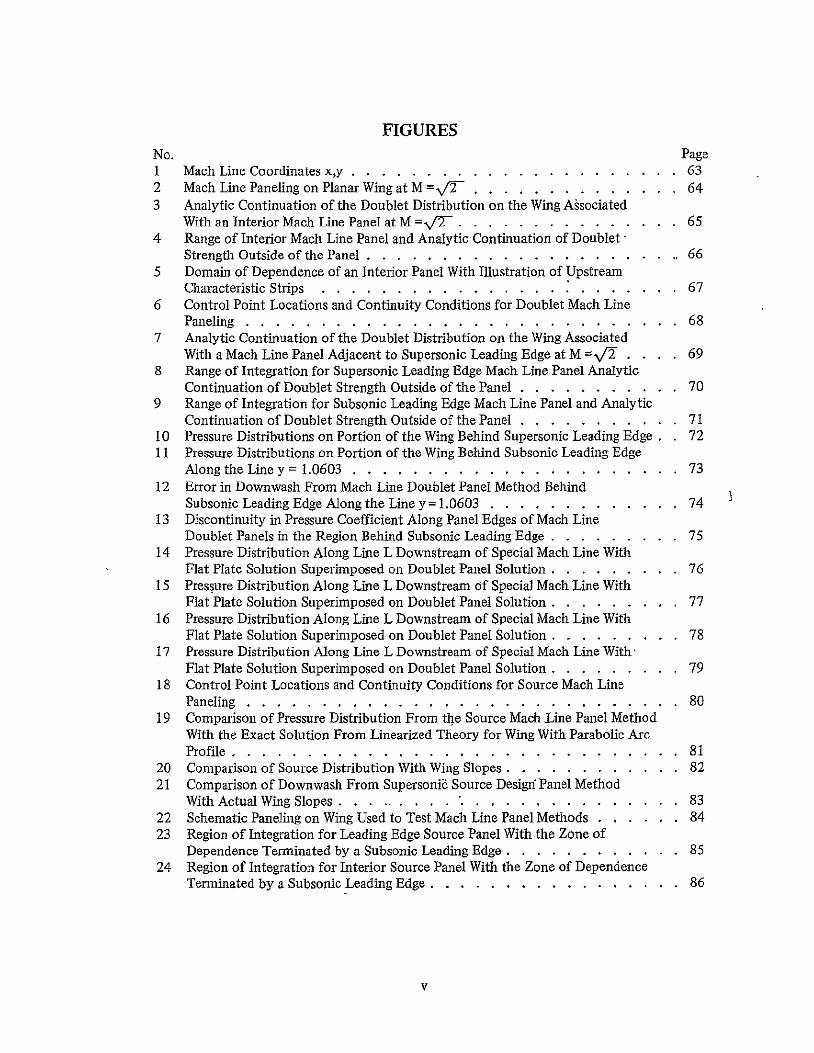
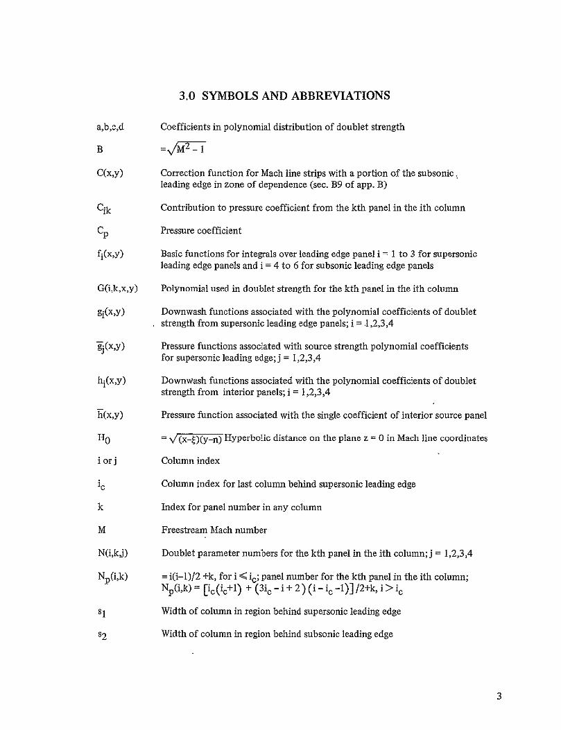
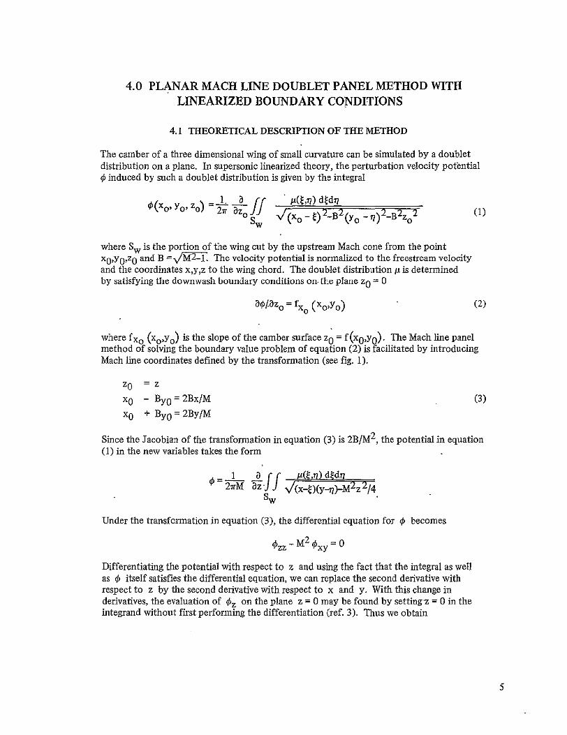
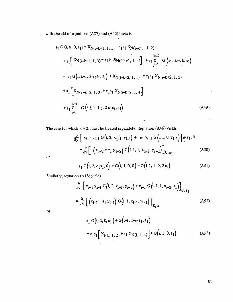
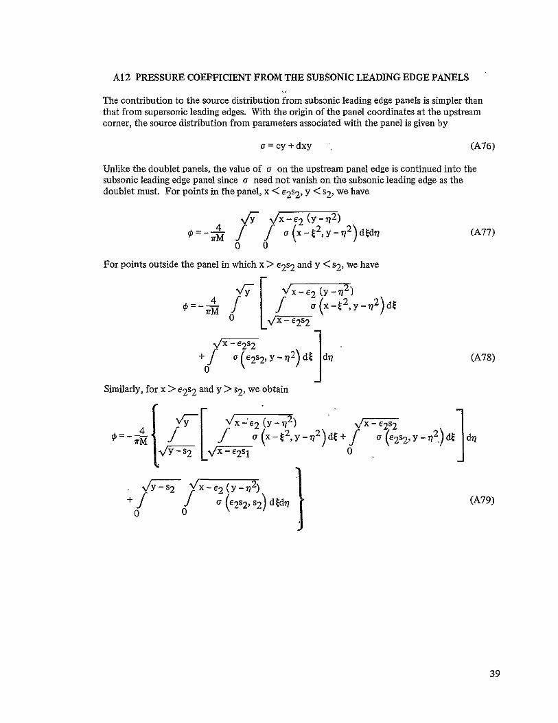
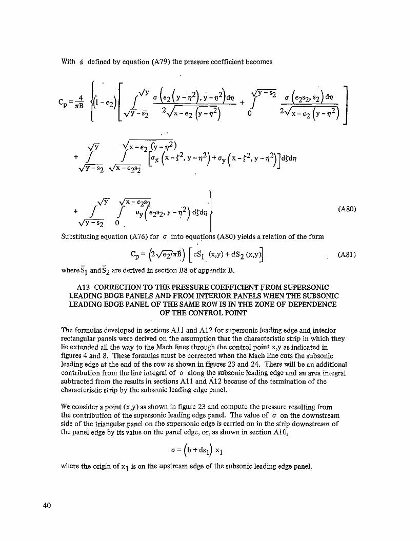
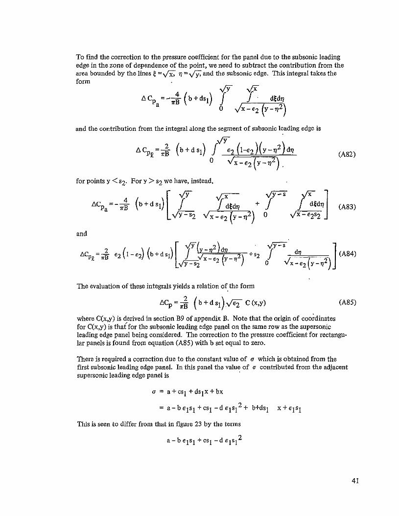
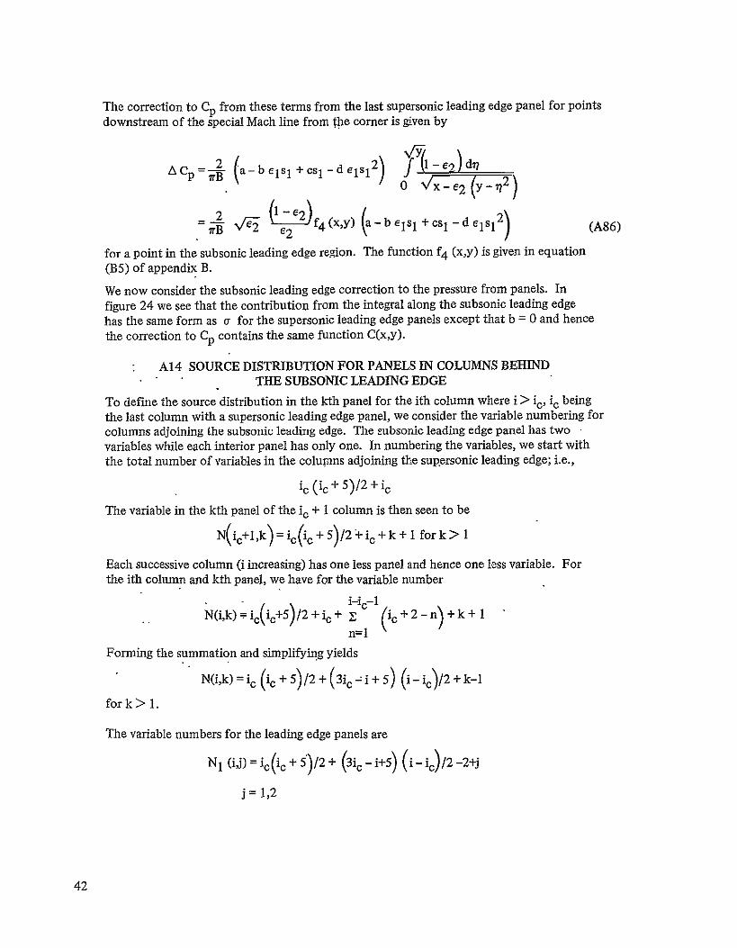
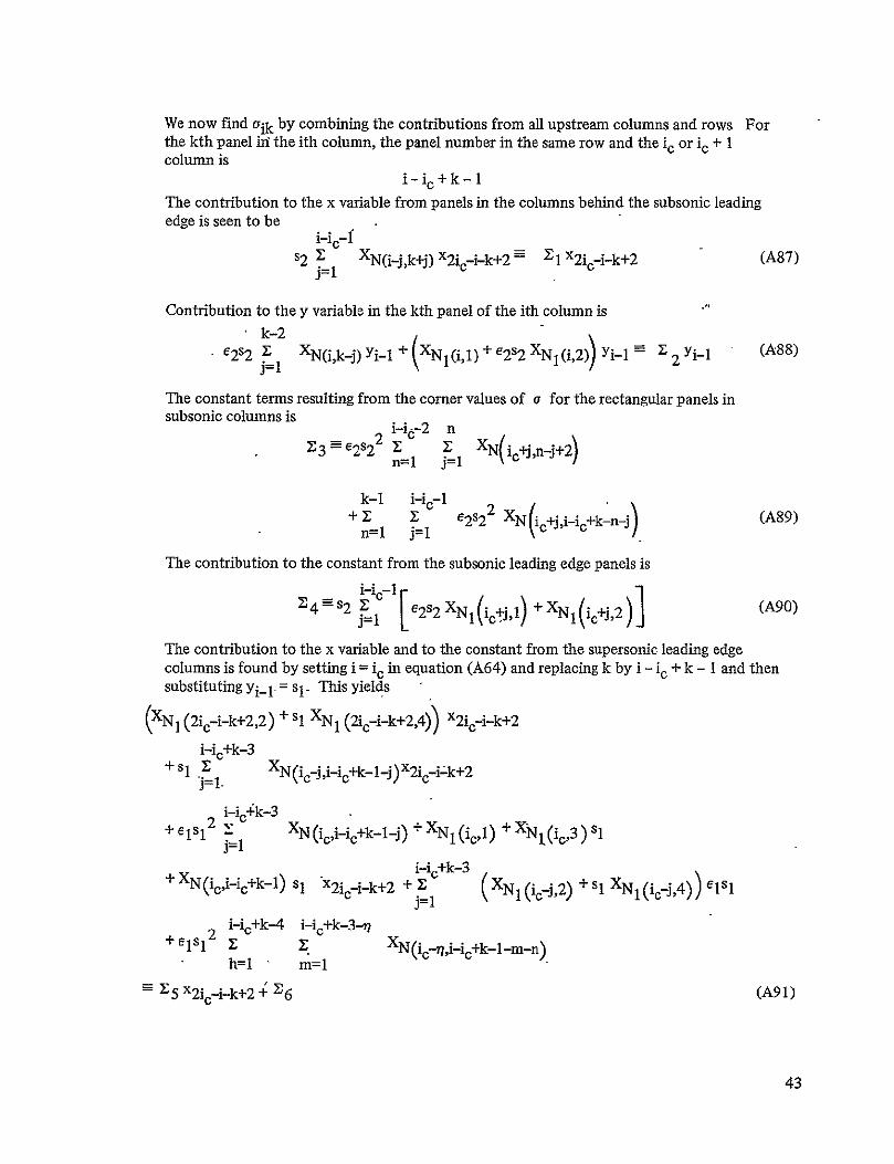
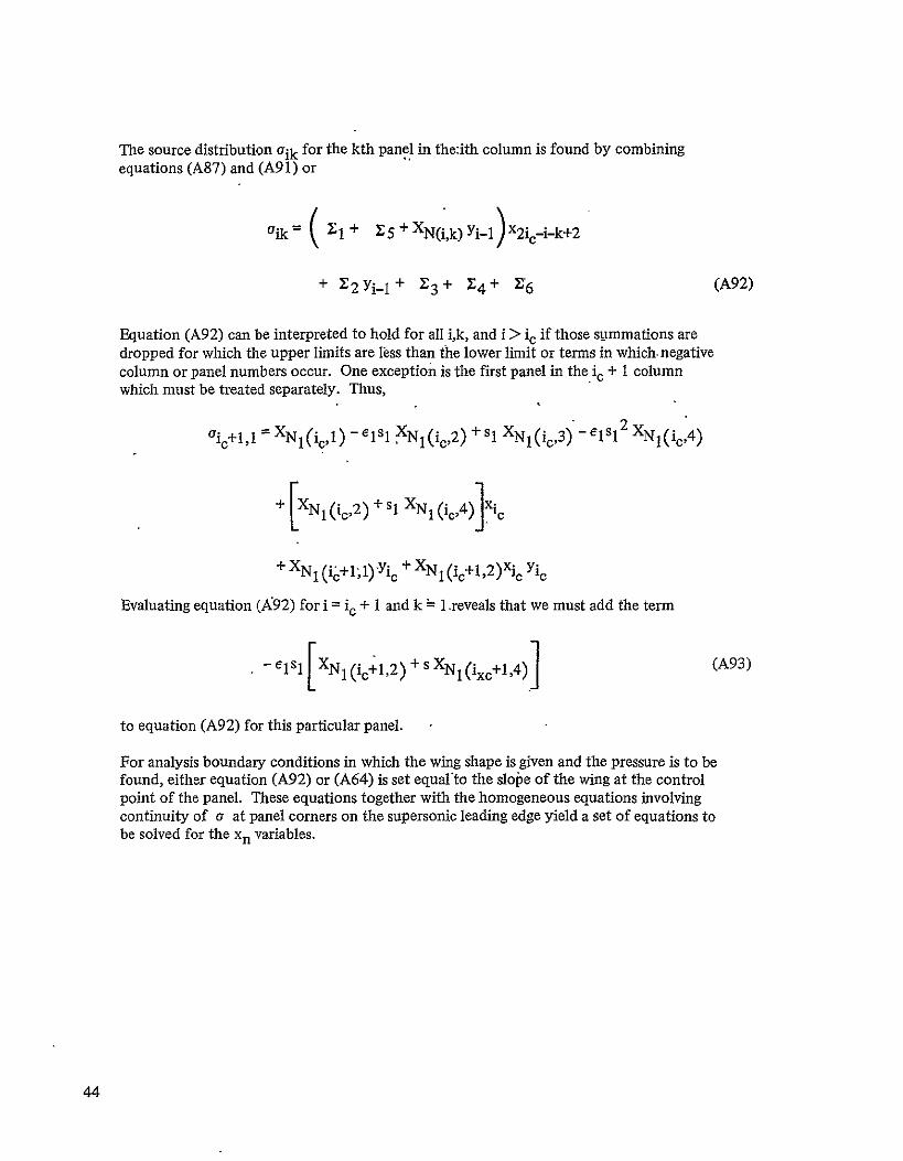
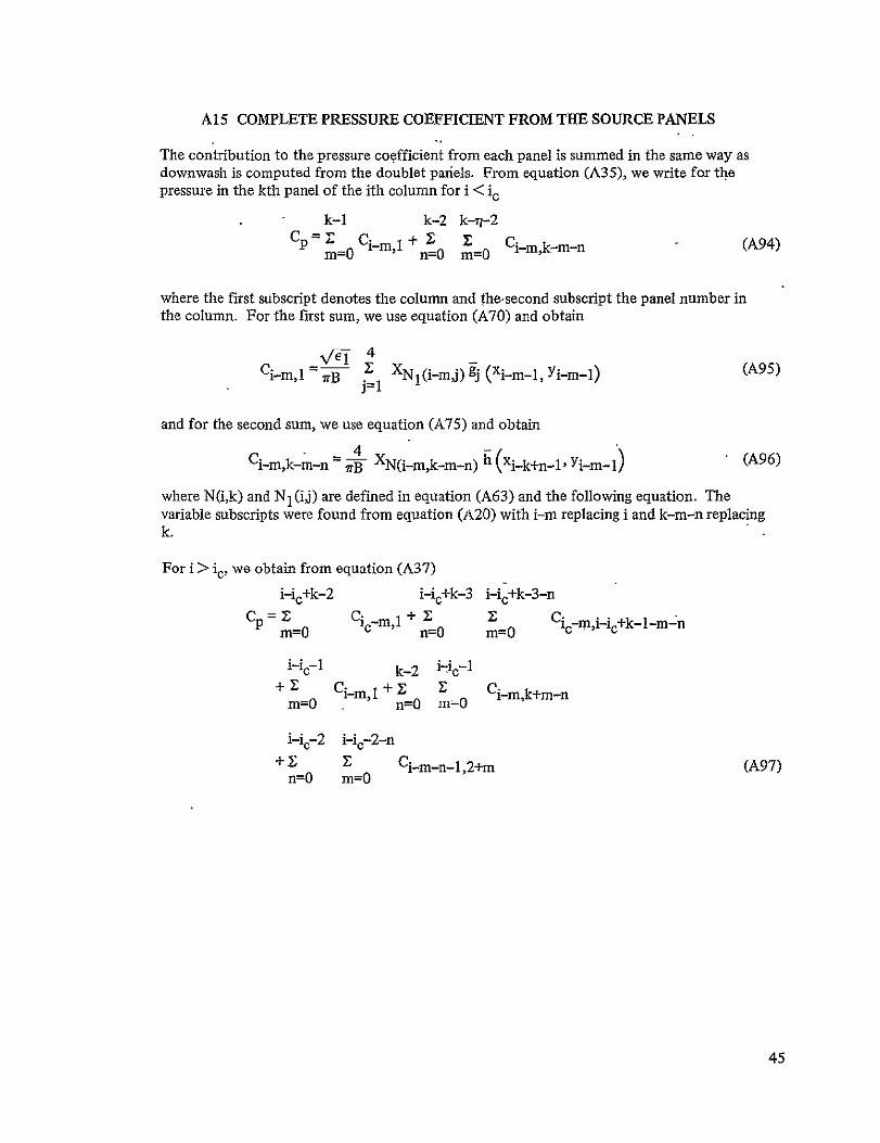
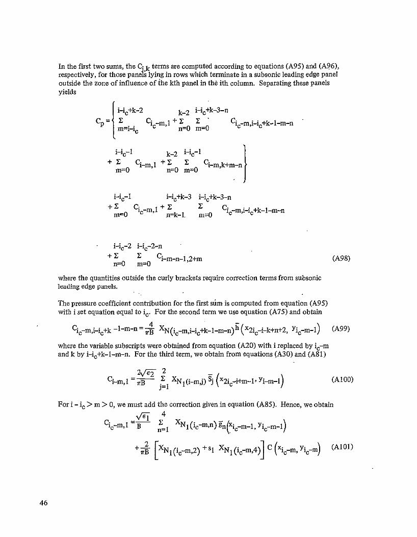
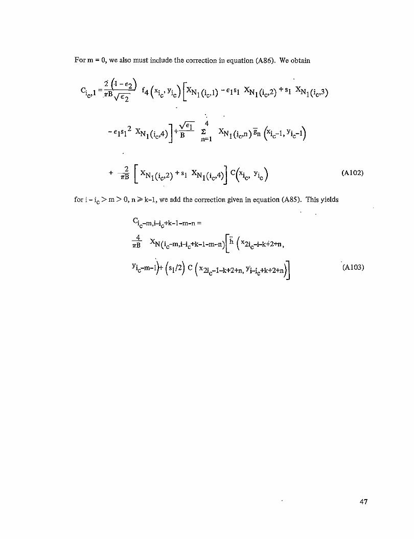
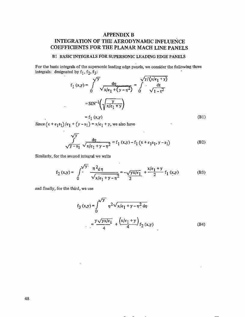
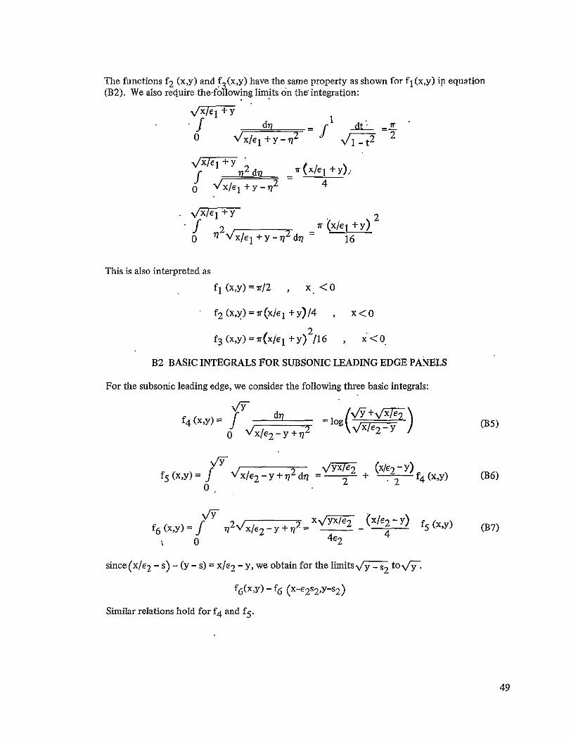
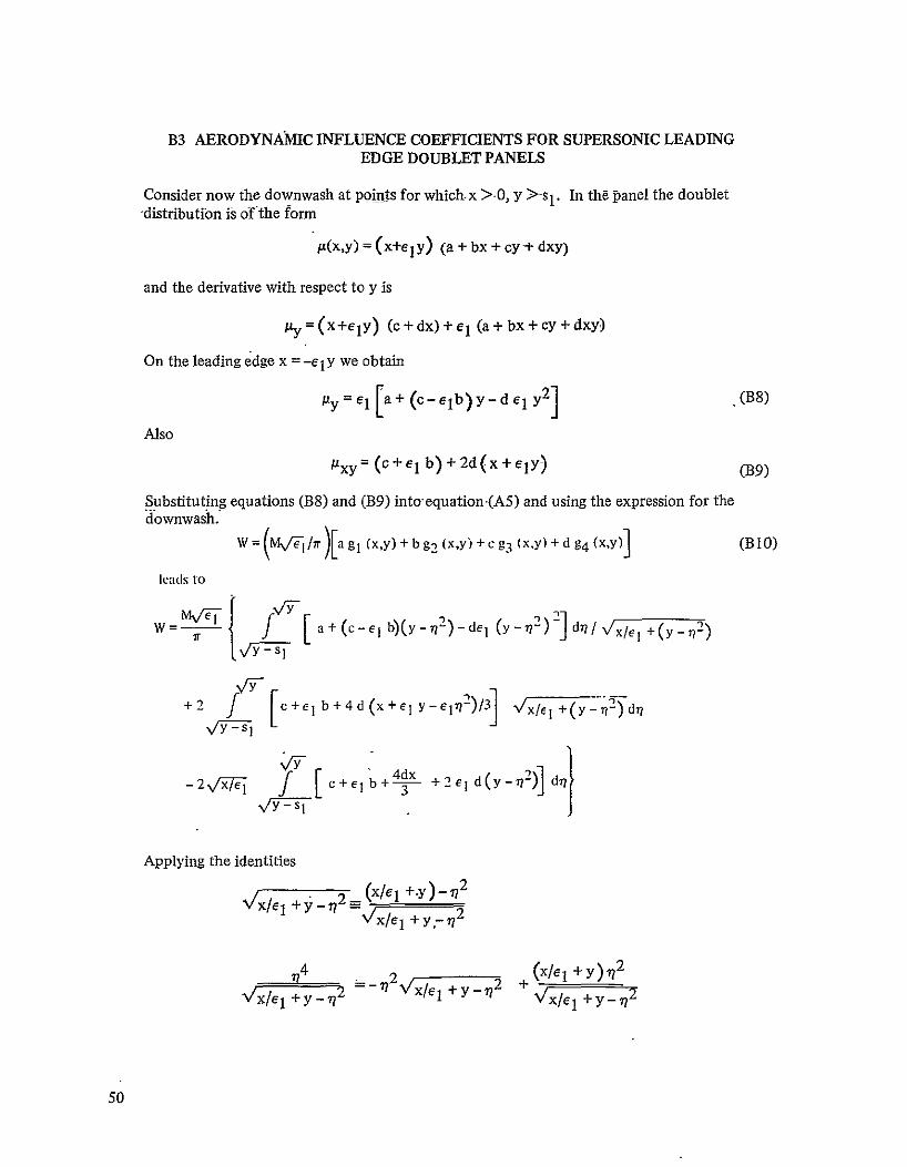
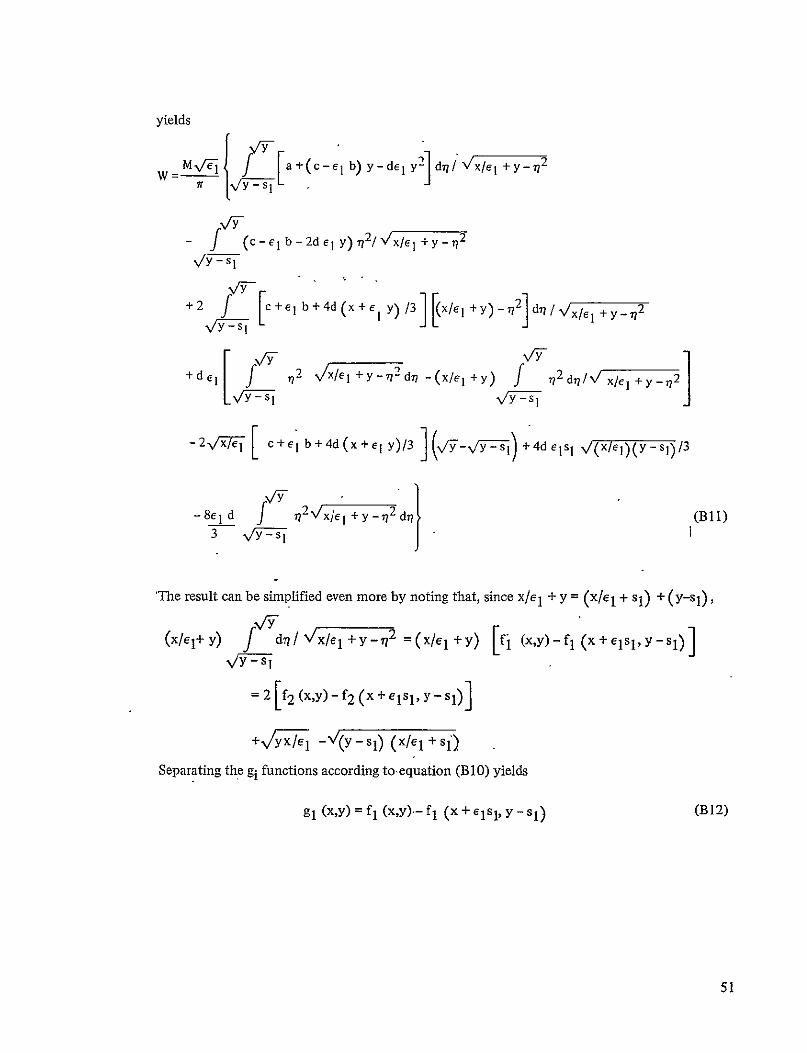
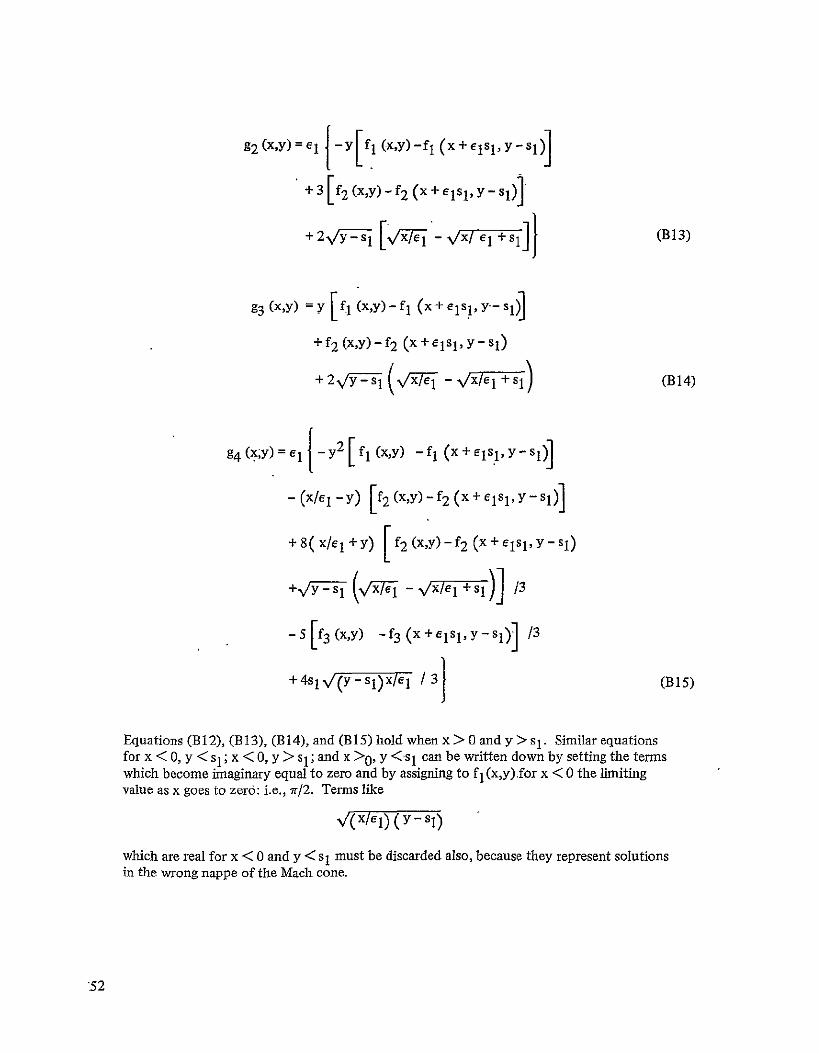
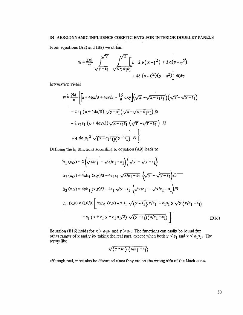
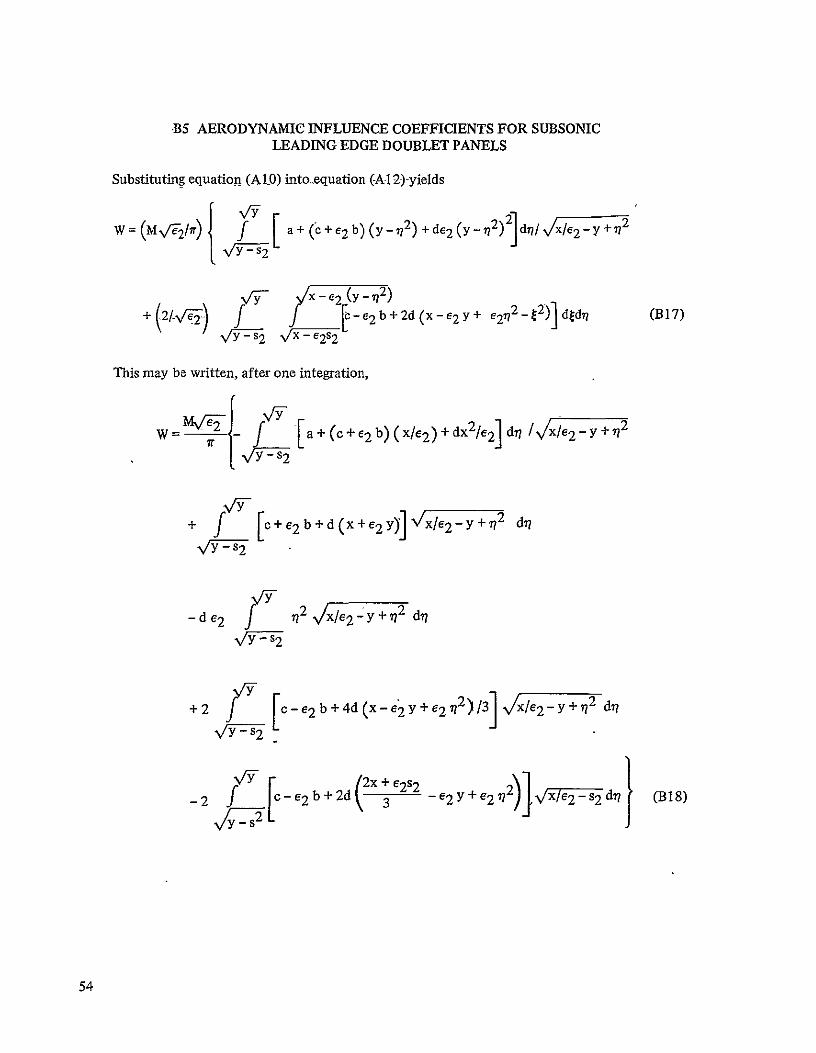
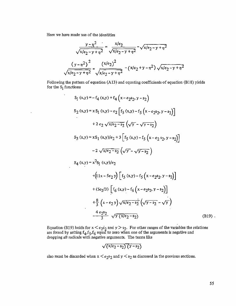
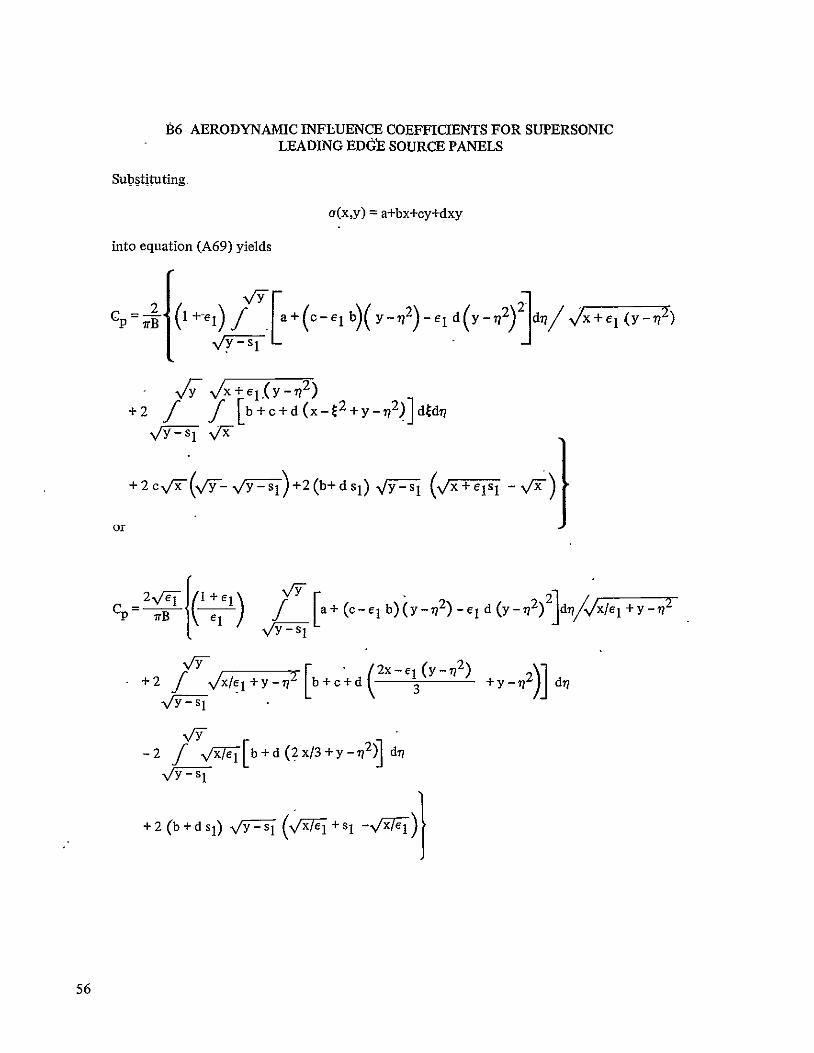
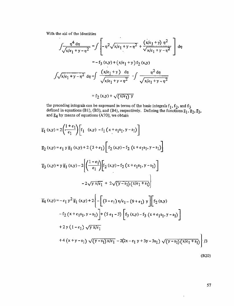
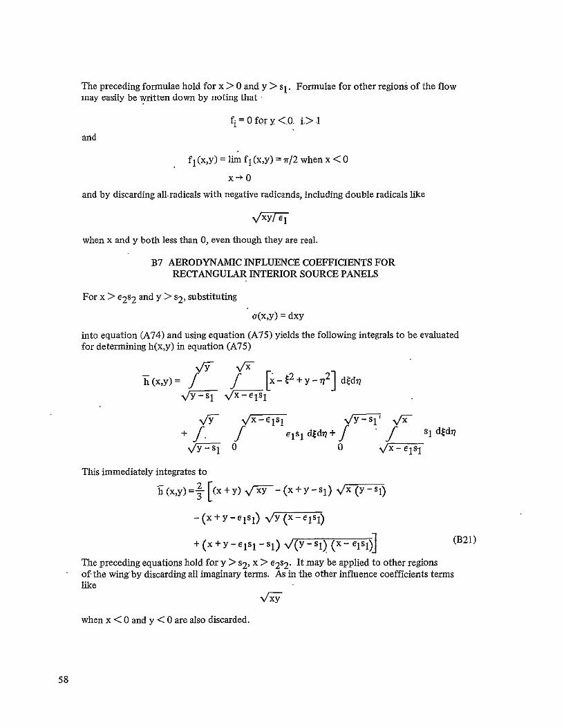
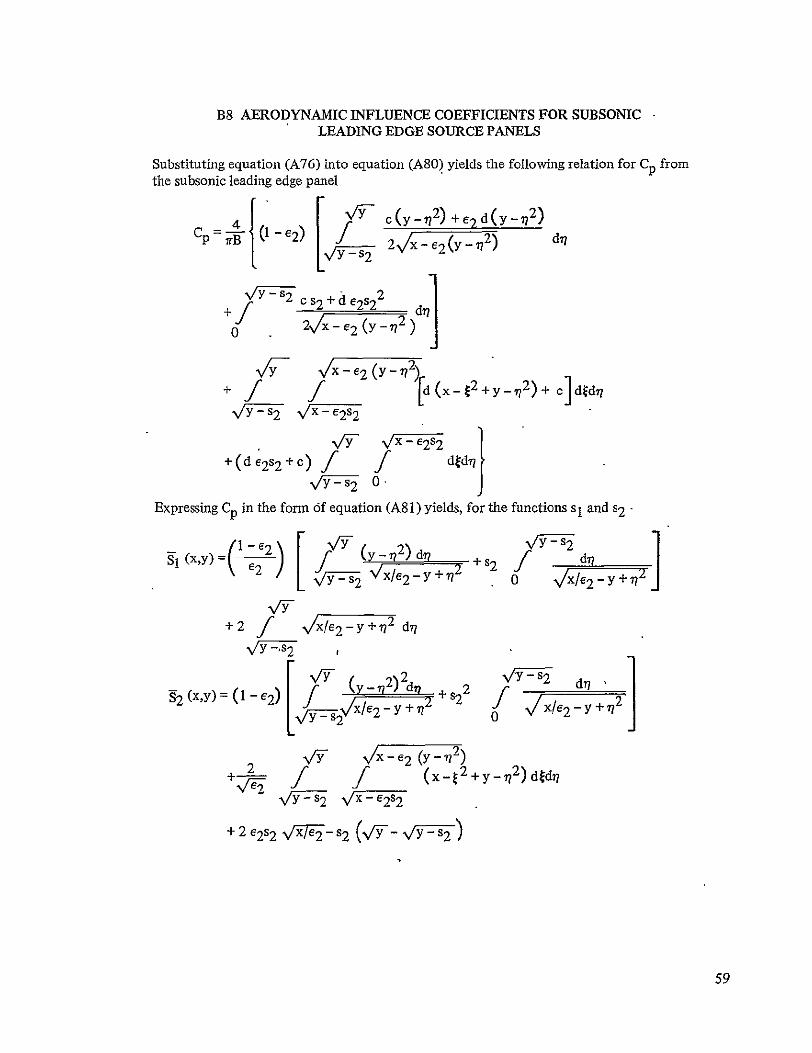
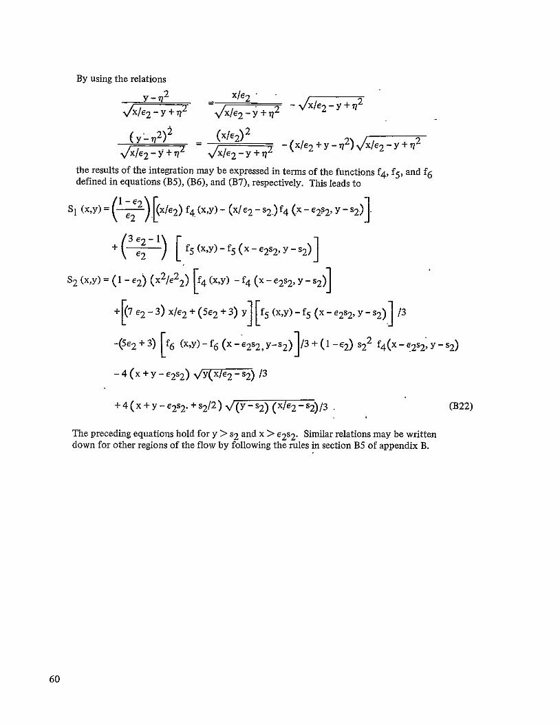
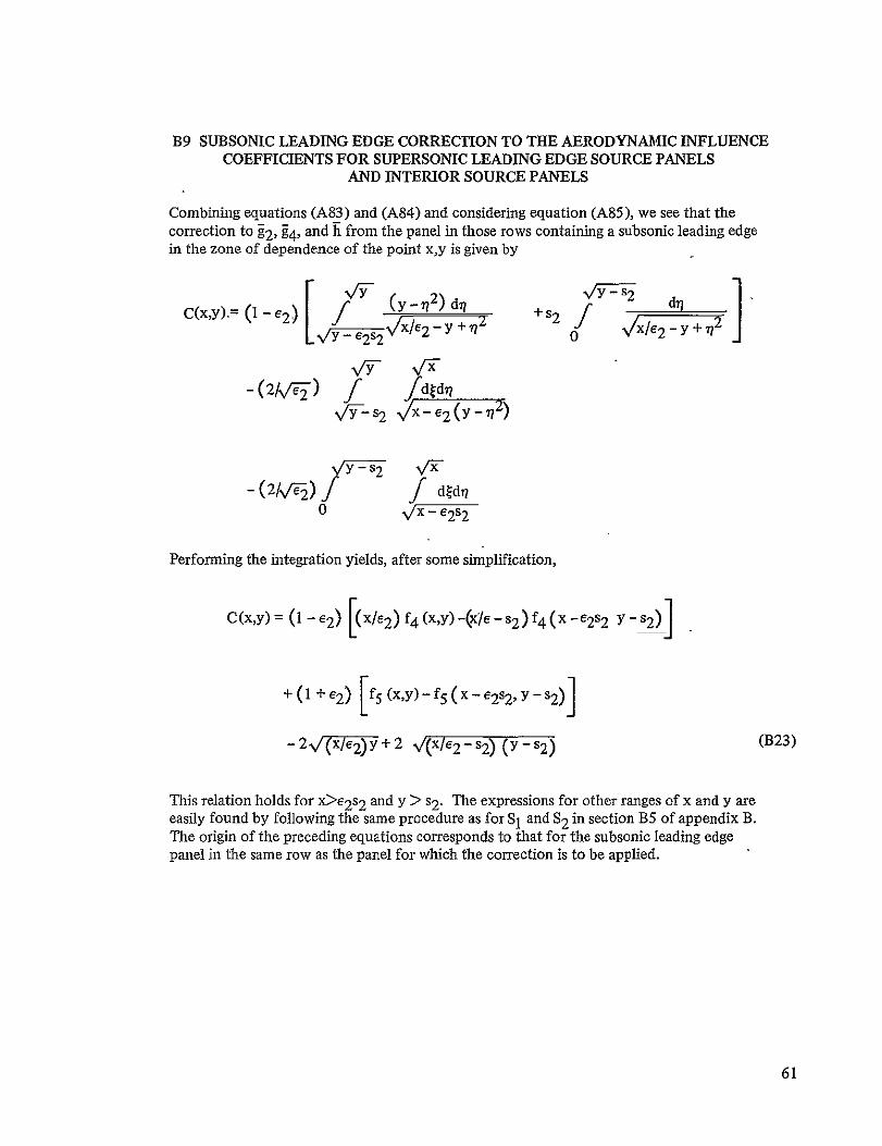
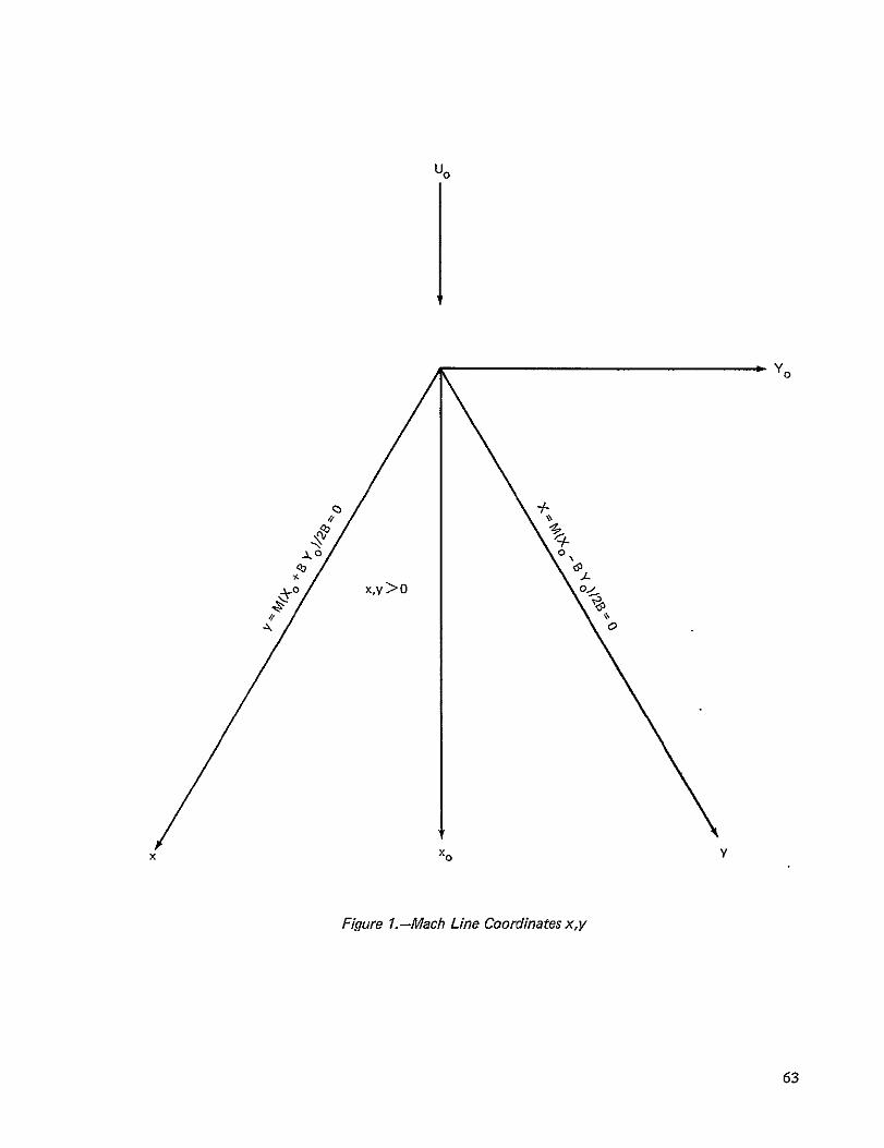
U0
Yo
S+ o ~xygtO
o
x y
Figure 1-Mach Line Coordinates xy
0
63
U0
Subsonic leading edge
leading edge
Figure 2-Mach Line Paneling on Planar Wing at M =shy
64
- U0
0V
Figure3-Analytic Continuationof the Doublet Distributionon the Wing Associated 7With an InteriorMach Line Panel atM =
65
U0
(o~sl) k (0si)
(eisi~o) (e1s1 O)
x
(a)Control Point x~y Inside the Panel W5Control Point xy Outside the Panel and on y Characteristic Strip
XFX xy Fixed point xy Variables of integration
(iso)(s)
xl
() Control Pointxy Outside the Panel (W)Control Point xy Outside the Panel and on x Characteristic Strip and Between Characteristic Strips
Figure 4-Range of Integration for Interior Mach Line Panel andAnalytic Continuation of Doublet Strength Outside of the Panel
66
U0
Figure 5-Domain of Dependence of an Interior Panel With Illustration of Upstream Characteristic Strips
67
-Ur
61 Y 0
x
0 Downwash control point (10 to 20 away from panel edges)
Continuity of normal derivative
Continuity of doublet gradient
Figure 6-ControlPoint Locations and Continuity Conditions for Doublet Mach Line Paneling
68
Uo
ft third degree polynomial
xA g constantant
Figure 7-Analytic Continuation of the Doublet Distribution on the Wing Associated With a Mach Line Panel Adjacent to Supersonic Leading Edge at M = 12
69
((-x-)) xy1N
(0sj 0
(x-xe I)
(a)Control Point y Inside the Panel m P(x )
~~tit=j t=P(Oyy
(b)Control Point xy Outside the Panel X and on y Characteristic Strip
o
) i-
x Y
X~
and on x Characteristic Strip K
(c) Control Point xy Outside the Panel ii (0 ~iiii_015i
700
(d) Control Point xy Outside the Panel x and Between Characteristic Strips
Figureamp-Rangeof integrationfor SupersonicLeading Edge Mach Line PanelAnalytic
Continuationof DoubletStrength Outside of the Panel
70
0
(62s 210) (62s2os2)
X U0
(a) Control Point xy Inside the Panel
0
(62s20) (e2 s2 s2 )
)
X x X X(b) Control Point xy Outside the Panel NIXand on x Characteristic Strip
Xfy
(c)Control Point xCy Outside Both Panel xxCharacteristic Strip anand
Figure 9-Range of Integration for Subsonic Leading Edge Mach Line Panel and Analytic Continuation of Doublet Strength Outside of the Panel
71
Uo
x
Parabolic arc profild
Sweep angle = 300 2i Z = 2t(1-Cy)(xl-x 2 )M = r C = 003
Y t = maximum camber
- Exact linearized solution
0 3 panels V1
A 10 panels
4
y =066667
3
Cpt 2
0 I I I I
0 10 20 30 40 50
-x
Figure ia-PressureDistributions on Portion of the Wing Behind Supersonic Leading Edge
72
U0
Parabolic arc airfoil
y
20
Linearized theory
-2 x
Panel method
-20 M = NF2 t = maximum camber
Figure 11-Pressure Distributions on Portion of the Wing Behind Subsonic Leading Edge Along the Line y = 10603
73
U 0
A
Parabolic arc airfoil T
V
40
20
wt 0 -10-20 x
-20
Figure 12-Error in Downwash From Mach Line Doublet Panel Method Behind Subsonic Leading Edge Along the Line y = 10603
74
-1 F30
20 Upstream side
t -
-pDownstreashyside
10
X
Ctheory A
0 1 2
Distance along line L in units of panel width
Figure 13-Discontinuity in Pressure Coefficient Along Panel Edges of Mach Line Doublet Panels in the Region Behind Subsonic Leading Edge
75
- --
Line L4 Uo
xAx r45
A3
Parabolic arc profileFreestream mach number =Nr2 Sweep angle = 30
Doublet panel method Exact linearized solution
Cpt 2
1
0 1 2 3 4 5 WAY
Figure 14-Pressure Distribution Along Line L Downstream ofSpecial Mach Line With Flat Plate Solution Superimposed on Doublet Panel Solution
76
4 U- Line L
0 ~xI6x = -40O
Axi i-- I I bull
Parabolic arc profile
x Freestream mach number =V2
Sweep angle = 30Q
Doublbt panel method Exact linearized solution
1
0 1 2 3 4 5
yAy
Figure 15-Pressure Distribution Along Line L Downstream of Special Mach Line With FlatPlateSolution Superimposed on Doublet PanelSolution
77
$ Parabolic are profile x Freestream mach number=
Sweep angle = 300
Cpt -Doublet panel-method Exact linearized solution
0shy
-1 III I
0 3 4 5 yAY
Figure 16-Pressure Distribution Along Line L Downstream ofSpecial Mach Line With Flat Plate Solution Superimposed on Doublet Panel Solution
78
3 Uo Line L xz~x = 0
-- 1
4shy I
2 Parabolic arc profile x Freestream mach number =V2-
Sweep angle = 300
Cpt
N Doublet panel method
- 1I I i
0 1 2 3 4 5
yAy
Figure 17-Pressure Distribution Along Line L Downstream ofSpecial Mach Line With Flat Plate Solution Superimposed on Doublet Panel Solution
79
U0
Analysis only
0 Design only
x
gt Continuity of source
Downwash (or pressure) control point Pressure control point only
(design boundary conditions)
Y
Figure 18-Control Point Locations and Continuity Conditions for Source Mach Line Paneling
80
4
Solution with six panels
Exact linearized
solution
3shy
13 1 20shy
000--- shy
cpt 2
15
135--- shy
120 --- shy
105
U0
05
0 -1 - 2 x
Figure 19-Comparisonof Pressure DistributionFrom the Source Mach Line Panel Method With the Exact Solution From Linearized Theory for Wing With Parabolic Arc Profile
81
18
16 1 6 ~ ~Source solution
14- Prescribed slope
12 131 shy
8o35--- 20
M =Nf-
x I
0 - 1 - 2 x
Figure 20-Comparison ofSource Distribution With Wing Slopes
05
82
U0
Biconvec airfoil 20 6t Mach number =-shy
0 13
--x-23 y 15 0
10x
y
- Wing slope-dydx
A DownwashW t Thickness ratio
10 30
V
Figure 21-Comparison of Downwash From Supersonic Source Design Panel Method With Actual Wing Slopes
83
U0
51 ~i CYc
Cp
7Q 7
-b 4 r
II
~ampr
M-V2
M=V
y
Figure 22-Schematic Paneling on Wing Used to Test Mach Line Panel Methods
84
U0
Supersonic leading edge
u - a ffk
(c + dx)
+ (b+ dy ) + cy + dxy
e a + bx +cs 1 + dxs1
S
ar (b+ds) (x+62 s2 )
a + y
qOx +Oy =
a=
ax +a
=
0a=
xy
(b+dsl)e 2 s2
Figure 23-Region of Integration for Leadfng Edge Source Panel With the Zone of Dependence Terminated by a Subsonic Leading Edge
85
x
U0
or= dx~y = ds x G dS lX
Cr del ilY
ax+ OF 0o + O =delS1x o=dje S
Figure 24-Region of Integration for Interior Source Panel With the Zone of Dependence Terminated by a Subsonic Leading Edge
86
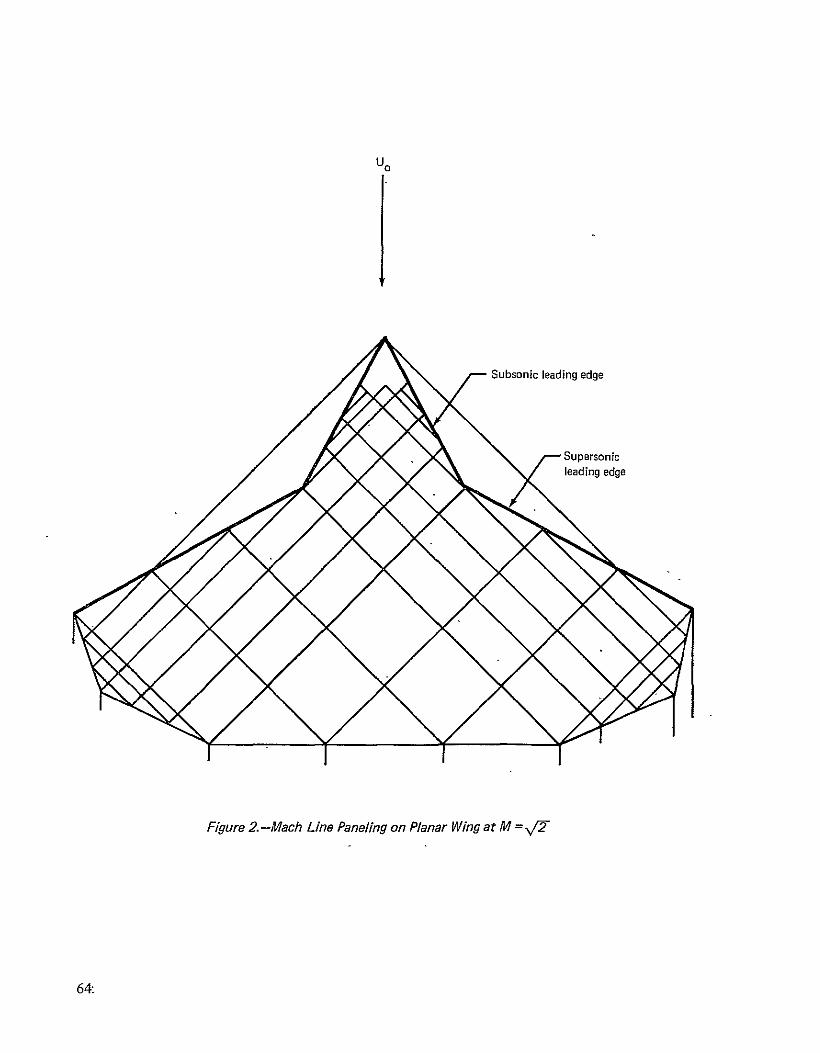
U0
Subsonic leading edge
leading edge
Figure 2-Mach Line Paneling on Planar Wing at M =shy
64
- U0
0V
Figure3-Analytic Continuationof the Doublet Distributionon the Wing Associated 7With an InteriorMach Line Panel atM =
65
U0
(o~sl) k (0si)
(eisi~o) (e1s1 O)
x
(a)Control Point x~y Inside the Panel W5Control Point xy Outside the Panel and on y Characteristic Strip
XFX xy Fixed point xy Variables of integration
(iso)(s)
xl
() Control Pointxy Outside the Panel (W)Control Point xy Outside the Panel and on x Characteristic Strip and Between Characteristic Strips
Figure 4-Range of Integration for Interior Mach Line Panel andAnalytic Continuation of Doublet Strength Outside of the Panel
66
U0
Figure 5-Domain of Dependence of an Interior Panel With Illustration of Upstream Characteristic Strips
67
-Ur
61 Y 0
x
0 Downwash control point (10 to 20 away from panel edges)
Continuity of normal derivative
Continuity of doublet gradient
Figure 6-ControlPoint Locations and Continuity Conditions for Doublet Mach Line Paneling
68
Uo
ft third degree polynomial
xA g constantant
Figure 7-Analytic Continuation of the Doublet Distribution on the Wing Associated With a Mach Line Panel Adjacent to Supersonic Leading Edge at M = 12
69
((-x-)) xy1N
(0sj 0
(x-xe I)
(a)Control Point y Inside the Panel m P(x )
~~tit=j t=P(Oyy
(b)Control Point xy Outside the Panel X and on y Characteristic Strip
o
) i-
x Y
X~
and on x Characteristic Strip K
(c) Control Point xy Outside the Panel ii (0 ~iiii_015i
700
(d) Control Point xy Outside the Panel x and Between Characteristic Strips
Figureamp-Rangeof integrationfor SupersonicLeading Edge Mach Line PanelAnalytic
Continuationof DoubletStrength Outside of the Panel
70
0
(62s 210) (62s2os2)
X U0
(a) Control Point xy Inside the Panel
0
(62s20) (e2 s2 s2 )
)
X x X X(b) Control Point xy Outside the Panel NIXand on x Characteristic Strip
Xfy
(c)Control Point xCy Outside Both Panel xxCharacteristic Strip anand
Figure 9-Range of Integration for Subsonic Leading Edge Mach Line Panel and Analytic Continuation of Doublet Strength Outside of the Panel
71
Uo
x
Parabolic arc profild
Sweep angle = 300 2i Z = 2t(1-Cy)(xl-x 2 )M = r C = 003
Y t = maximum camber
- Exact linearized solution
0 3 panels V1
A 10 panels
4
y =066667
3
Cpt 2
0 I I I I
0 10 20 30 40 50
-x
Figure ia-PressureDistributions on Portion of the Wing Behind Supersonic Leading Edge
72
U0
Parabolic arc airfoil
y
20
Linearized theory
-2 x
Panel method
-20 M = NF2 t = maximum camber
Figure 11-Pressure Distributions on Portion of the Wing Behind Subsonic Leading Edge Along the Line y = 10603
73
U 0
A
Parabolic arc airfoil T
V
40
20
wt 0 -10-20 x
-20
Figure 12-Error in Downwash From Mach Line Doublet Panel Method Behind Subsonic Leading Edge Along the Line y = 10603
74
-1 F30
20 Upstream side
t -
-pDownstreashyside
10
X
Ctheory A
0 1 2
Distance along line L in units of panel width
Figure 13-Discontinuity in Pressure Coefficient Along Panel Edges of Mach Line Doublet Panels in the Region Behind Subsonic Leading Edge
75
- --
Line L4 Uo
xAx r45
A3
Parabolic arc profileFreestream mach number =Nr2 Sweep angle = 30
Doublet panel method Exact linearized solution
Cpt 2
1
0 1 2 3 4 5 WAY
Figure 14-Pressure Distribution Along Line L Downstream ofSpecial Mach Line With Flat Plate Solution Superimposed on Doublet Panel Solution
76
4 U- Line L
0 ~xI6x = -40O
Axi i-- I I bull
Parabolic arc profile
x Freestream mach number =V2
Sweep angle = 30Q
Doublbt panel method Exact linearized solution
1
0 1 2 3 4 5
yAy
Figure 15-Pressure Distribution Along Line L Downstream of Special Mach Line With FlatPlateSolution Superimposed on Doublet PanelSolution
77
$ Parabolic are profile x Freestream mach number=
Sweep angle = 300
Cpt -Doublet panel-method Exact linearized solution
0shy
-1 III I
0 3 4 5 yAY
Figure 16-Pressure Distribution Along Line L Downstream ofSpecial Mach Line With Flat Plate Solution Superimposed on Doublet Panel Solution
78
3 Uo Line L xz~x = 0
-- 1
4shy I
2 Parabolic arc profile x Freestream mach number =V2-
Sweep angle = 300
Cpt
N Doublet panel method
- 1I I i
0 1 2 3 4 5
yAy
Figure 17-Pressure Distribution Along Line L Downstream ofSpecial Mach Line With Flat Plate Solution Superimposed on Doublet Panel Solution
79
U0
Analysis only
0 Design only
x
gt Continuity of source
Downwash (or pressure) control point Pressure control point only
(design boundary conditions)
Y
Figure 18-Control Point Locations and Continuity Conditions for Source Mach Line Paneling
80
4
Solution with six panels
Exact linearized
solution
3shy
13 1 20shy
000--- shy
cpt 2
15
135--- shy
120 --- shy
105
U0
05
0 -1 - 2 x
Figure 19-Comparisonof Pressure DistributionFrom the Source Mach Line Panel Method With the Exact Solution From Linearized Theory for Wing With Parabolic Arc Profile
81
18
16 1 6 ~ ~Source solution
14- Prescribed slope
12 131 shy
8o35--- 20
M =Nf-
x I
0 - 1 - 2 x
Figure 20-Comparison ofSource Distribution With Wing Slopes
05
82
U0
Biconvec airfoil 20 6t Mach number =-shy
0 13
--x-23 y 15 0
10x
y
- Wing slope-dydx
A DownwashW t Thickness ratio
10 30
V
Figure 21-Comparison of Downwash From Supersonic Source Design Panel Method With Actual Wing Slopes
83
U0
51 ~i CYc
Cp
7Q 7
-b 4 r
II
~ampr
M-V2
M=V
y
Figure 22-Schematic Paneling on Wing Used to Test Mach Line Panel Methods
84
U0
Supersonic leading edge
u - a ffk
(c + dx)
+ (b+ dy ) + cy + dxy
e a + bx +cs 1 + dxs1
S
ar (b+ds) (x+62 s2 )
a + y
qOx +Oy =
a=
ax +a
=
0a=
xy
(b+dsl)e 2 s2
Figure 23-Region of Integration for Leadfng Edge Source Panel With the Zone of Dependence Terminated by a Subsonic Leading Edge
85
x
U0
or= dx~y = ds x G dS lX
Cr del ilY
ax+ OF 0o + O =delS1x o=dje S
Figure 24-Region of Integration for Interior Source Panel With the Zone of Dependence Terminated by a Subsonic Leading Edge
86
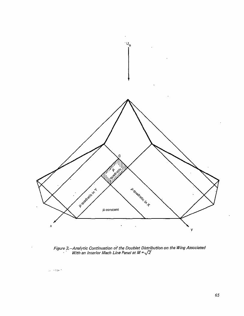
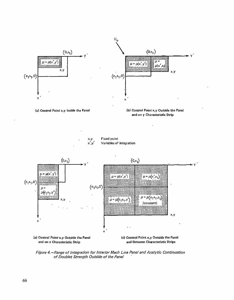
U0
(o~sl) k (0si)
(eisi~o) (e1s1 O)
x
(a)Control Point x~y Inside the Panel W5Control Point xy Outside the Panel and on y Characteristic Strip
XFX xy Fixed point xy Variables of integration
(iso)(s)
xl
() Control Pointxy Outside the Panel (W)Control Point xy Outside the Panel and on x Characteristic Strip and Between Characteristic Strips
Figure 4-Range of Integration for Interior Mach Line Panel andAnalytic Continuation of Doublet Strength Outside of the Panel
66
U0
Figure 5-Domain of Dependence of an Interior Panel With Illustration of Upstream Characteristic Strips
67
-Ur
61 Y 0
x
0 Downwash control point (10 to 20 away from panel edges)
Continuity of normal derivative
Continuity of doublet gradient
Figure 6-ControlPoint Locations and Continuity Conditions for Doublet Mach Line Paneling
68
Uo
ft third degree polynomial
xA g constantant
Figure 7-Analytic Continuation of the Doublet Distribution on the Wing Associated With a Mach Line Panel Adjacent to Supersonic Leading Edge at M = 12
69
((-x-)) xy1N
(0sj 0
(x-xe I)
(a)Control Point y Inside the Panel m P(x )
~~tit=j t=P(Oyy
(b)Control Point xy Outside the Panel X and on y Characteristic Strip
o
) i-
x Y
X~
and on x Characteristic Strip K
(c) Control Point xy Outside the Panel ii (0 ~iiii_015i
700
(d) Control Point xy Outside the Panel x and Between Characteristic Strips
Figureamp-Rangeof integrationfor SupersonicLeading Edge Mach Line PanelAnalytic
Continuationof DoubletStrength Outside of the Panel
70
0
(62s 210) (62s2os2)
X U0
(a) Control Point xy Inside the Panel
0
(62s20) (e2 s2 s2 )
)
X x X X(b) Control Point xy Outside the Panel NIXand on x Characteristic Strip
Xfy
(c)Control Point xCy Outside Both Panel xxCharacteristic Strip anand
Figure 9-Range of Integration for Subsonic Leading Edge Mach Line Panel and Analytic Continuation of Doublet Strength Outside of the Panel
71
Uo
x
Parabolic arc profild
Sweep angle = 300 2i Z = 2t(1-Cy)(xl-x 2 )M = r C = 003
Y t = maximum camber
- Exact linearized solution
0 3 panels V1
A 10 panels
4
y =066667
3
Cpt 2
0 I I I I
0 10 20 30 40 50
-x
Figure ia-PressureDistributions on Portion of the Wing Behind Supersonic Leading Edge
72
U0
Parabolic arc airfoil
y
20
Linearized theory
-2 x
Panel method
-20 M = NF2 t = maximum camber
Figure 11-Pressure Distributions on Portion of the Wing Behind Subsonic Leading Edge Along the Line y = 10603
73
U 0
A
Parabolic arc airfoil T
V
40
20
wt 0 -10-20 x
-20
Figure 12-Error in Downwash From Mach Line Doublet Panel Method Behind Subsonic Leading Edge Along the Line y = 10603
74
-1 F30
20 Upstream side
t -
-pDownstreashyside
10
X
Ctheory A
0 1 2
Distance along line L in units of panel width
Figure 13-Discontinuity in Pressure Coefficient Along Panel Edges of Mach Line Doublet Panels in the Region Behind Subsonic Leading Edge
75
- --
Line L4 Uo
xAx r45
A3
Parabolic arc profileFreestream mach number =Nr2 Sweep angle = 30
Doublet panel method Exact linearized solution
Cpt 2
1
0 1 2 3 4 5 WAY
Figure 14-Pressure Distribution Along Line L Downstream ofSpecial Mach Line With Flat Plate Solution Superimposed on Doublet Panel Solution
76
4 U- Line L
0 ~xI6x = -40O
Axi i-- I I bull
Parabolic arc profile
x Freestream mach number =V2
Sweep angle = 30Q
Doublbt panel method Exact linearized solution
1
0 1 2 3 4 5
yAy
Figure 15-Pressure Distribution Along Line L Downstream of Special Mach Line With FlatPlateSolution Superimposed on Doublet PanelSolution
77
$ Parabolic are profile x Freestream mach number=
Sweep angle = 300
Cpt -Doublet panel-method Exact linearized solution
0shy
-1 III I
0 3 4 5 yAY
Figure 16-Pressure Distribution Along Line L Downstream ofSpecial Mach Line With Flat Plate Solution Superimposed on Doublet Panel Solution
78
3 Uo Line L xz~x = 0
-- 1
4shy I
2 Parabolic arc profile x Freestream mach number =V2-
Sweep angle = 300
Cpt
N Doublet panel method
- 1I I i
0 1 2 3 4 5
yAy
Figure 17-Pressure Distribution Along Line L Downstream ofSpecial Mach Line With Flat Plate Solution Superimposed on Doublet Panel Solution
79
U0
Analysis only
0 Design only
x
gt Continuity of source
Downwash (or pressure) control point Pressure control point only
(design boundary conditions)
Y
Figure 18-Control Point Locations and Continuity Conditions for Source Mach Line Paneling
80
4
Solution with six panels
Exact linearized
solution
3shy
13 1 20shy
000--- shy
cpt 2
15
135--- shy
120 --- shy
105
U0
05
0 -1 - 2 x
Figure 19-Comparisonof Pressure DistributionFrom the Source Mach Line Panel Method With the Exact Solution From Linearized Theory for Wing With Parabolic Arc Profile
81
18
16 1 6 ~ ~Source solution
14- Prescribed slope
12 131 shy
8o35--- 20
M =Nf-
x I
0 - 1 - 2 x
Figure 20-Comparison ofSource Distribution With Wing Slopes
05
82
U0
Biconvec airfoil 20 6t Mach number =-shy
0 13
--x-23 y 15 0
10x
y
- Wing slope-dydx
A DownwashW t Thickness ratio
10 30
V
Figure 21-Comparison of Downwash From Supersonic Source Design Panel Method With Actual Wing Slopes
83
U0
51 ~i CYc
Cp
7Q 7
-b 4 r
II
~ampr
M-V2
M=V
y
Figure 22-Schematic Paneling on Wing Used to Test Mach Line Panel Methods
84
U0
Supersonic leading edge
u - a ffk
(c + dx)
+ (b+ dy ) + cy + dxy
e a + bx +cs 1 + dxs1
S
ar (b+ds) (x+62 s2 )
a + y
qOx +Oy =
a=
ax +a
=
0a=
xy
(b+dsl)e 2 s2
Figure 23-Region of Integration for Leadfng Edge Source Panel With the Zone of Dependence Terminated by a Subsonic Leading Edge
85
x
U0
or= dx~y = ds x G dS lX
Cr del ilY
ax+ OF 0o + O =delS1x o=dje S
Figure 24-Region of Integration for Interior Source Panel With the Zone of Dependence Terminated by a Subsonic Leading Edge
86
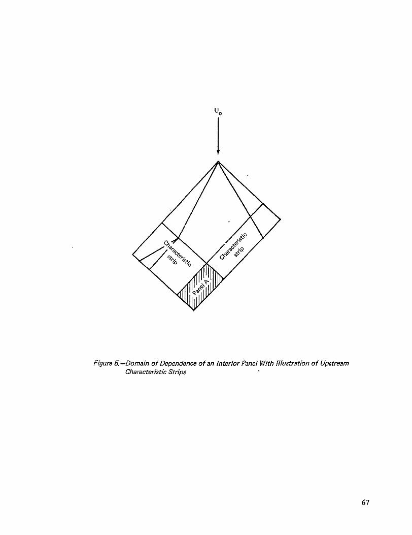
U0
Figure 5-Domain of Dependence of an Interior Panel With Illustration of Upstream Characteristic Strips
67
-Ur
61 Y 0
x
0 Downwash control point (10 to 20 away from panel edges)
Continuity of normal derivative
Continuity of doublet gradient
Figure 6-ControlPoint Locations and Continuity Conditions for Doublet Mach Line Paneling
68
Uo
ft third degree polynomial
xA g constantant
Figure 7-Analytic Continuation of the Doublet Distribution on the Wing Associated With a Mach Line Panel Adjacent to Supersonic Leading Edge at M = 12
69
((-x-)) xy1N
(0sj 0
(x-xe I)
(a)Control Point y Inside the Panel m P(x )
~~tit=j t=P(Oyy
(b)Control Point xy Outside the Panel X and on y Characteristic Strip
o
) i-
x Y
X~
and on x Characteristic Strip K
(c) Control Point xy Outside the Panel ii (0 ~iiii_015i
700
(d) Control Point xy Outside the Panel x and Between Characteristic Strips
Figureamp-Rangeof integrationfor SupersonicLeading Edge Mach Line PanelAnalytic
Continuationof DoubletStrength Outside of the Panel
70
0
(62s 210) (62s2os2)
X U0
(a) Control Point xy Inside the Panel
0
(62s20) (e2 s2 s2 )
)
X x X X(b) Control Point xy Outside the Panel NIXand on x Characteristic Strip
Xfy
(c)Control Point xCy Outside Both Panel xxCharacteristic Strip anand
Figure 9-Range of Integration for Subsonic Leading Edge Mach Line Panel and Analytic Continuation of Doublet Strength Outside of the Panel
71
Uo
x
Parabolic arc profild
Sweep angle = 300 2i Z = 2t(1-Cy)(xl-x 2 )M = r C = 003
Y t = maximum camber
- Exact linearized solution
0 3 panels V1
A 10 panels
4
y =066667
3
Cpt 2
0 I I I I
0 10 20 30 40 50
-x
Figure ia-PressureDistributions on Portion of the Wing Behind Supersonic Leading Edge
72
U0
Parabolic arc airfoil
y
20
Linearized theory
-2 x
Panel method
-20 M = NF2 t = maximum camber
Figure 11-Pressure Distributions on Portion of the Wing Behind Subsonic Leading Edge Along the Line y = 10603
73
U 0
A
Parabolic arc airfoil T
V
40
20
wt 0 -10-20 x
-20
Figure 12-Error in Downwash From Mach Line Doublet Panel Method Behind Subsonic Leading Edge Along the Line y = 10603
74
-1 F30
20 Upstream side
t -
-pDownstreashyside
10
X
Ctheory A
0 1 2
Distance along line L in units of panel width
Figure 13-Discontinuity in Pressure Coefficient Along Panel Edges of Mach Line Doublet Panels in the Region Behind Subsonic Leading Edge
75
- --
Line L4 Uo
xAx r45
A3
Parabolic arc profileFreestream mach number =Nr2 Sweep angle = 30
Doublet panel method Exact linearized solution
Cpt 2
1
0 1 2 3 4 5 WAY
Figure 14-Pressure Distribution Along Line L Downstream ofSpecial Mach Line With Flat Plate Solution Superimposed on Doublet Panel Solution
76
4 U- Line L
0 ~xI6x = -40O
Axi i-- I I bull
Parabolic arc profile
x Freestream mach number =V2
Sweep angle = 30Q
Doublbt panel method Exact linearized solution
1
0 1 2 3 4 5
yAy
Figure 15-Pressure Distribution Along Line L Downstream of Special Mach Line With FlatPlateSolution Superimposed on Doublet PanelSolution
77
$ Parabolic are profile x Freestream mach number=
Sweep angle = 300
Cpt -Doublet panel-method Exact linearized solution
0shy
-1 III I
0 3 4 5 yAY
Figure 16-Pressure Distribution Along Line L Downstream ofSpecial Mach Line With Flat Plate Solution Superimposed on Doublet Panel Solution
78
3 Uo Line L xz~x = 0
-- 1
4shy I
2 Parabolic arc profile x Freestream mach number =V2-
Sweep angle = 300
Cpt
N Doublet panel method
- 1I I i
0 1 2 3 4 5
yAy
Figure 17-Pressure Distribution Along Line L Downstream ofSpecial Mach Line With Flat Plate Solution Superimposed on Doublet Panel Solution
79
U0
Analysis only
0 Design only
x
gt Continuity of source
Downwash (or pressure) control point Pressure control point only
(design boundary conditions)
Y
Figure 18-Control Point Locations and Continuity Conditions for Source Mach Line Paneling
80
4
Solution with six panels
Exact linearized
solution
3shy
13 1 20shy
000--- shy
cpt 2
15
135--- shy
120 --- shy
105
U0
05
0 -1 - 2 x
Figure 19-Comparisonof Pressure DistributionFrom the Source Mach Line Panel Method With the Exact Solution From Linearized Theory for Wing With Parabolic Arc Profile
81
18
16 1 6 ~ ~Source solution
14- Prescribed slope
12 131 shy
8o35--- 20
M =Nf-
x I
0 - 1 - 2 x
Figure 20-Comparison ofSource Distribution With Wing Slopes
05
82
U0
Biconvec airfoil 20 6t Mach number =-shy
0 13
--x-23 y 15 0
10x
y
- Wing slope-dydx
A DownwashW t Thickness ratio
10 30
V
Figure 21-Comparison of Downwash From Supersonic Source Design Panel Method With Actual Wing Slopes
83
U0
51 ~i CYc
Cp
7Q 7
-b 4 r
II
~ampr
M-V2
M=V
y
Figure 22-Schematic Paneling on Wing Used to Test Mach Line Panel Methods
84
U0
Supersonic leading edge
u - a ffk
(c + dx)
+ (b+ dy ) + cy + dxy
e a + bx +cs 1 + dxs1
S
ar (b+ds) (x+62 s2 )
a + y
qOx +Oy =
a=
ax +a
=
0a=
xy
(b+dsl)e 2 s2
Figure 23-Region of Integration for Leadfng Edge Source Panel With the Zone of Dependence Terminated by a Subsonic Leading Edge
85
x
U0
or= dx~y = ds x G dS lX
Cr del ilY
ax+ OF 0o + O =delS1x o=dje S
Figure 24-Region of Integration for Interior Source Panel With the Zone of Dependence Terminated by a Subsonic Leading Edge
86
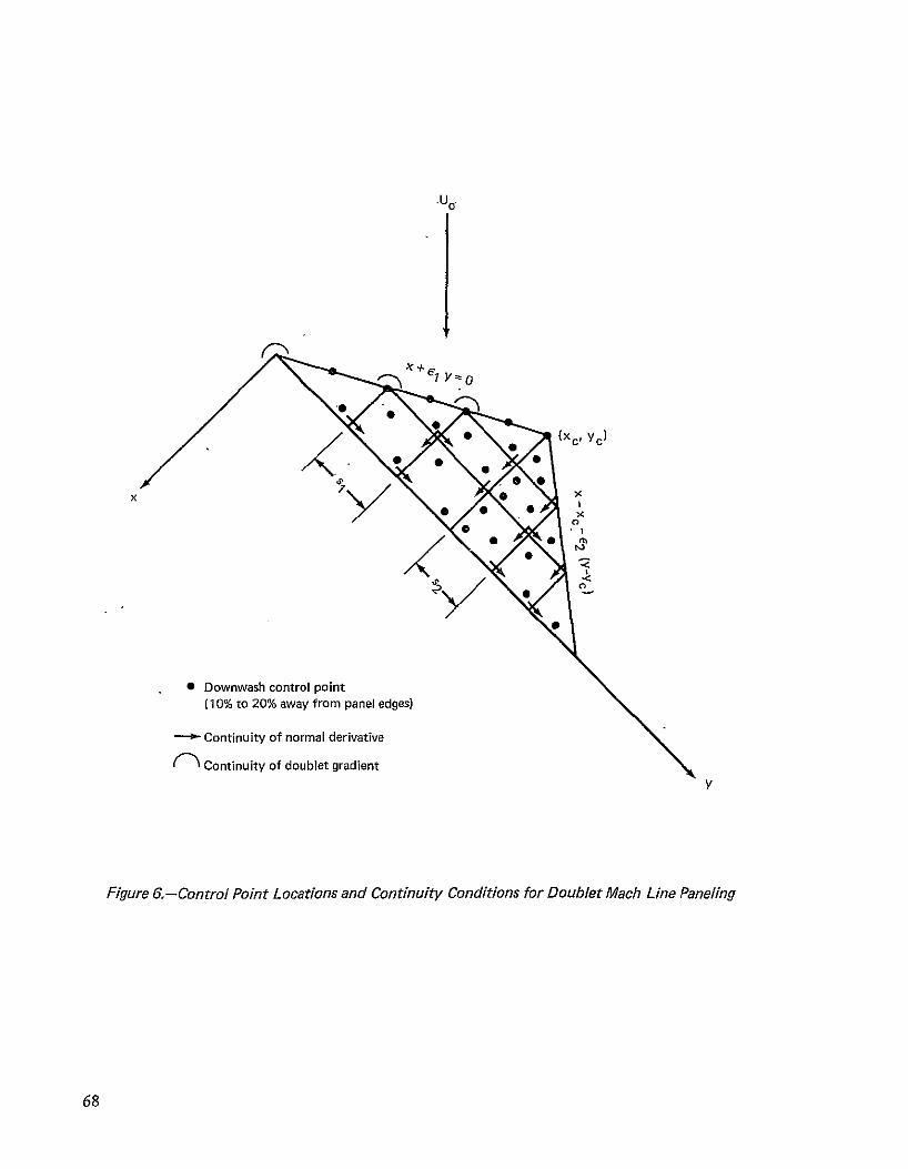
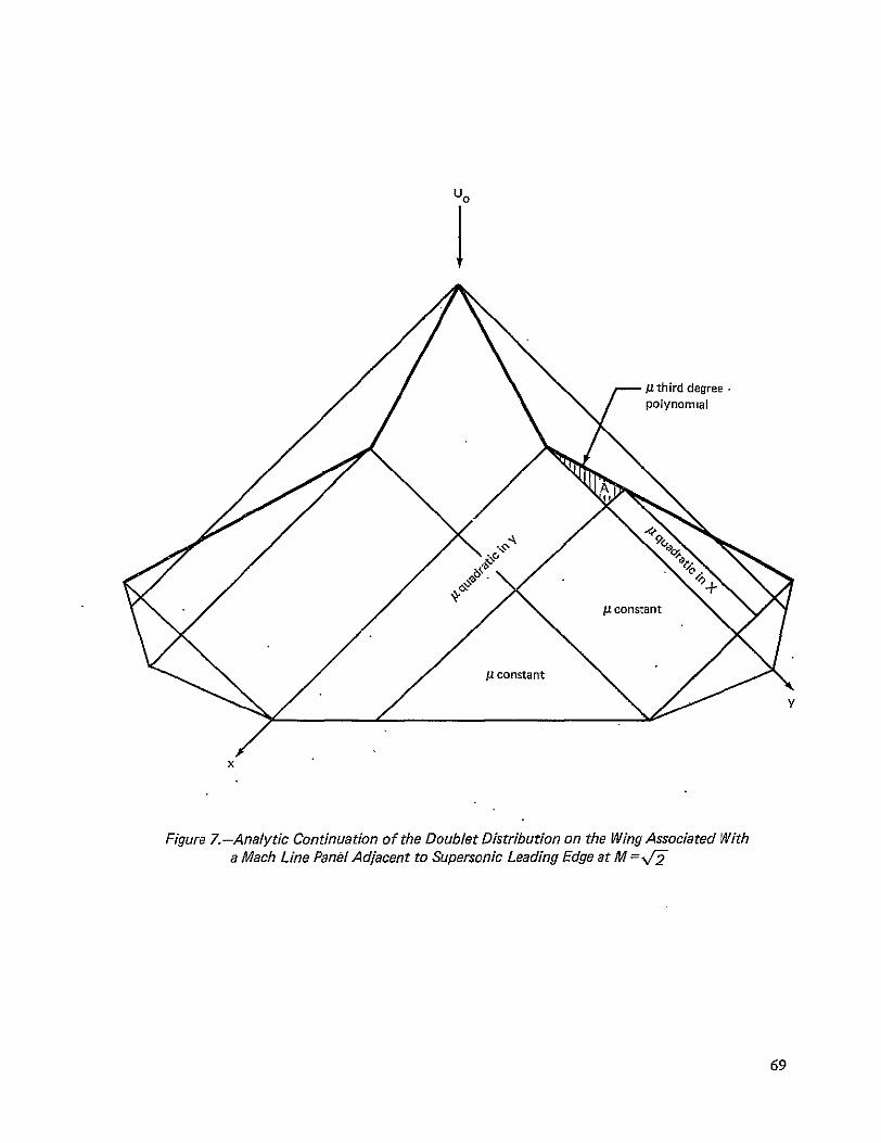
Uo
ft third degree polynomial
xA g constantant
Figure 7-Analytic Continuation of the Doublet Distribution on the Wing Associated With a Mach Line Panel Adjacent to Supersonic Leading Edge at M = 12
69
((-x-)) xy1N
(0sj 0
(x-xe I)
(a)Control Point y Inside the Panel m P(x )
~~tit=j t=P(Oyy
(b)Control Point xy Outside the Panel X and on y Characteristic Strip
o
) i-
x Y
X~
and on x Characteristic Strip K
(c) Control Point xy Outside the Panel ii (0 ~iiii_015i
700
(d) Control Point xy Outside the Panel x and Between Characteristic Strips
Figureamp-Rangeof integrationfor SupersonicLeading Edge Mach Line PanelAnalytic
Continuationof DoubletStrength Outside of the Panel
70
0
(62s 210) (62s2os2)
X U0
(a) Control Point xy Inside the Panel
0
(62s20) (e2 s2 s2 )
)
X x X X(b) Control Point xy Outside the Panel NIXand on x Characteristic Strip
Xfy
(c)Control Point xCy Outside Both Panel xxCharacteristic Strip anand
Figure 9-Range of Integration for Subsonic Leading Edge Mach Line Panel and Analytic Continuation of Doublet Strength Outside of the Panel
71
Uo
x
Parabolic arc profild
Sweep angle = 300 2i Z = 2t(1-Cy)(xl-x 2 )M = r C = 003
Y t = maximum camber
- Exact linearized solution
0 3 panels V1
A 10 panels
4
y =066667
3
Cpt 2
0 I I I I
0 10 20 30 40 50
-x
Figure ia-PressureDistributions on Portion of the Wing Behind Supersonic Leading Edge
72
U0
Parabolic arc airfoil
y
20
Linearized theory
-2 x
Panel method
-20 M = NF2 t = maximum camber
Figure 11-Pressure Distributions on Portion of the Wing Behind Subsonic Leading Edge Along the Line y = 10603
73
U 0
A
Parabolic arc airfoil T
V
40
20
wt 0 -10-20 x
-20
Figure 12-Error in Downwash From Mach Line Doublet Panel Method Behind Subsonic Leading Edge Along the Line y = 10603
74
-1 F30
20 Upstream side
t -
-pDownstreashyside
10
X
Ctheory A
0 1 2
Distance along line L in units of panel width
Figure 13-Discontinuity in Pressure Coefficient Along Panel Edges of Mach Line Doublet Panels in the Region Behind Subsonic Leading Edge
75
- --
Line L4 Uo
xAx r45
A3
Parabolic arc profileFreestream mach number =Nr2 Sweep angle = 30
Doublet panel method Exact linearized solution
Cpt 2
1
0 1 2 3 4 5 WAY
Figure 14-Pressure Distribution Along Line L Downstream ofSpecial Mach Line With Flat Plate Solution Superimposed on Doublet Panel Solution
76
4 U- Line L
0 ~xI6x = -40O
Axi i-- I I bull
Parabolic arc profile
x Freestream mach number =V2
Sweep angle = 30Q
Doublbt panel method Exact linearized solution
1
0 1 2 3 4 5
yAy
Figure 15-Pressure Distribution Along Line L Downstream of Special Mach Line With FlatPlateSolution Superimposed on Doublet PanelSolution
77
$ Parabolic are profile x Freestream mach number=
Sweep angle = 300
Cpt -Doublet panel-method Exact linearized solution
0shy
-1 III I
0 3 4 5 yAY
Figure 16-Pressure Distribution Along Line L Downstream ofSpecial Mach Line With Flat Plate Solution Superimposed on Doublet Panel Solution
78
3 Uo Line L xz~x = 0
-- 1
4shy I
2 Parabolic arc profile x Freestream mach number =V2-
Sweep angle = 300
Cpt
N Doublet panel method
- 1I I i
0 1 2 3 4 5
yAy
Figure 17-Pressure Distribution Along Line L Downstream ofSpecial Mach Line With Flat Plate Solution Superimposed on Doublet Panel Solution
79
U0
Analysis only
0 Design only
x
gt Continuity of source
Downwash (or pressure) control point Pressure control point only
(design boundary conditions)
Y
Figure 18-Control Point Locations and Continuity Conditions for Source Mach Line Paneling
80
4
Solution with six panels
Exact linearized
solution
3shy
13 1 20shy
000--- shy
cpt 2
15
135--- shy
120 --- shy
105
U0
05
0 -1 - 2 x
Figure 19-Comparisonof Pressure DistributionFrom the Source Mach Line Panel Method With the Exact Solution From Linearized Theory for Wing With Parabolic Arc Profile
81
18
16 1 6 ~ ~Source solution
14- Prescribed slope
12 131 shy
8o35--- 20
M =Nf-
x I
0 - 1 - 2 x
Figure 20-Comparison ofSource Distribution With Wing Slopes
05
82
U0
Biconvec airfoil 20 6t Mach number =-shy
0 13
--x-23 y 15 0
10x
y
- Wing slope-dydx
A DownwashW t Thickness ratio
10 30
V
Figure 21-Comparison of Downwash From Supersonic Source Design Panel Method With Actual Wing Slopes
83
U0
51 ~i CYc
Cp
7Q 7
-b 4 r
II
~ampr
M-V2
M=V
y
Figure 22-Schematic Paneling on Wing Used to Test Mach Line Panel Methods
84
U0
Supersonic leading edge
u - a ffk
(c + dx)
+ (b+ dy ) + cy + dxy
e a + bx +cs 1 + dxs1
S
ar (b+ds) (x+62 s2 )
a + y
qOx +Oy =
a=
ax +a
=
0a=
xy
(b+dsl)e 2 s2
Figure 23-Region of Integration for Leadfng Edge Source Panel With the Zone of Dependence Terminated by a Subsonic Leading Edge
85
x
U0
or= dx~y = ds x G dS lX
Cr del ilY
ax+ OF 0o + O =delS1x o=dje S
Figure 24-Region of Integration for Interior Source Panel With the Zone of Dependence Terminated by a Subsonic Leading Edge
86
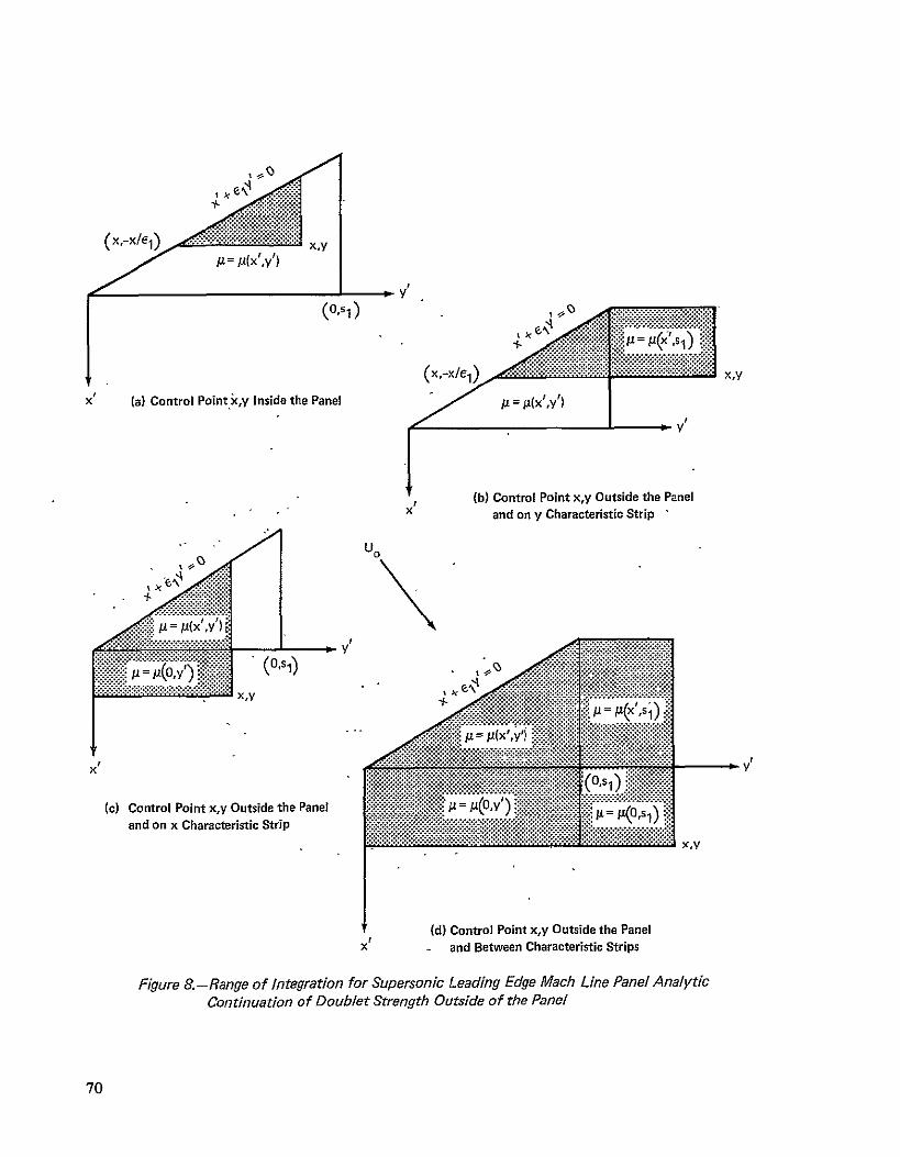
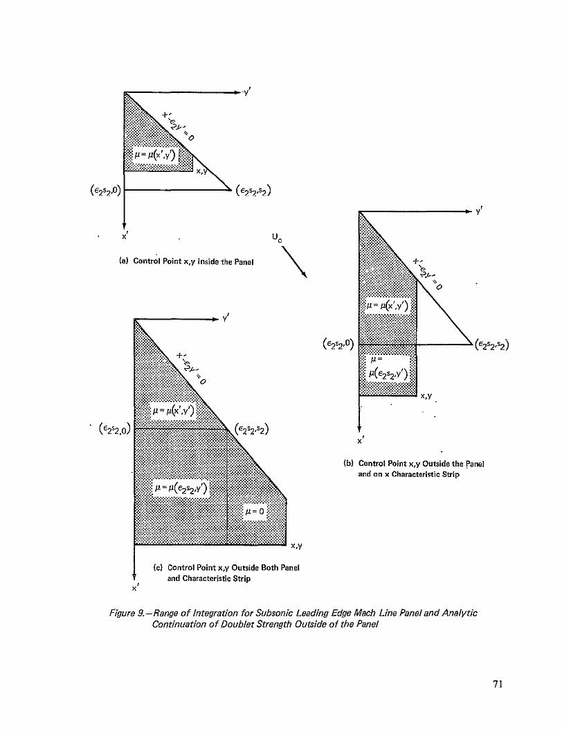
0
(62s 210) (62s2os2)
X U0
(a) Control Point xy Inside the Panel
0
(62s20) (e2 s2 s2 )
)
X x X X(b) Control Point xy Outside the Panel NIXand on x Characteristic Strip
Xfy
(c)Control Point xCy Outside Both Panel xxCharacteristic Strip anand
Figure 9-Range of Integration for Subsonic Leading Edge Mach Line Panel and Analytic Continuation of Doublet Strength Outside of the Panel
71
Uo
x
Parabolic arc profild
Sweep angle = 300 2i Z = 2t(1-Cy)(xl-x 2 )M = r C = 003
Y t = maximum camber
- Exact linearized solution
0 3 panels V1
A 10 panels
4
y =066667
3
Cpt 2
0 I I I I
0 10 20 30 40 50
-x
Figure ia-PressureDistributions on Portion of the Wing Behind Supersonic Leading Edge
72
U0
Parabolic arc airfoil
y
20
Linearized theory
-2 x
Panel method
-20 M = NF2 t = maximum camber
Figure 11-Pressure Distributions on Portion of the Wing Behind Subsonic Leading Edge Along the Line y = 10603
73
U 0
A
Parabolic arc airfoil T
V
40
20
wt 0 -10-20 x
-20
Figure 12-Error in Downwash From Mach Line Doublet Panel Method Behind Subsonic Leading Edge Along the Line y = 10603
74
-1 F30
20 Upstream side
t -
-pDownstreashyside
10
X
Ctheory A
0 1 2
Distance along line L in units of panel width
Figure 13-Discontinuity in Pressure Coefficient Along Panel Edges of Mach Line Doublet Panels in the Region Behind Subsonic Leading Edge
75
- --
Line L4 Uo
xAx r45
A3
Parabolic arc profileFreestream mach number =Nr2 Sweep angle = 30
Doublet panel method Exact linearized solution
Cpt 2
1
0 1 2 3 4 5 WAY
Figure 14-Pressure Distribution Along Line L Downstream ofSpecial Mach Line With Flat Plate Solution Superimposed on Doublet Panel Solution
76
4 U- Line L
0 ~xI6x = -40O
Axi i-- I I bull
Parabolic arc profile
x Freestream mach number =V2
Sweep angle = 30Q
Doublbt panel method Exact linearized solution
1
0 1 2 3 4 5
yAy
Figure 15-Pressure Distribution Along Line L Downstream of Special Mach Line With FlatPlateSolution Superimposed on Doublet PanelSolution
77
$ Parabolic are profile x Freestream mach number=
Sweep angle = 300
Cpt -Doublet panel-method Exact linearized solution
0shy
-1 III I
0 3 4 5 yAY
Figure 16-Pressure Distribution Along Line L Downstream ofSpecial Mach Line With Flat Plate Solution Superimposed on Doublet Panel Solution
78
3 Uo Line L xz~x = 0
-- 1
4shy I
2 Parabolic arc profile x Freestream mach number =V2-
Sweep angle = 300
Cpt
N Doublet panel method
- 1I I i
0 1 2 3 4 5
yAy
Figure 17-Pressure Distribution Along Line L Downstream ofSpecial Mach Line With Flat Plate Solution Superimposed on Doublet Panel Solution
79
U0
Analysis only
0 Design only
x
gt Continuity of source
Downwash (or pressure) control point Pressure control point only
(design boundary conditions)
Y
Figure 18-Control Point Locations and Continuity Conditions for Source Mach Line Paneling
80
4
Solution with six panels
Exact linearized
solution
3shy
13 1 20shy
000--- shy
cpt 2
15
135--- shy
120 --- shy
105
U0
05
0 -1 - 2 x
Figure 19-Comparisonof Pressure DistributionFrom the Source Mach Line Panel Method With the Exact Solution From Linearized Theory for Wing With Parabolic Arc Profile
81
18
16 1 6 ~ ~Source solution
14- Prescribed slope
12 131 shy
8o35--- 20
M =Nf-
x I
0 - 1 - 2 x
Figure 20-Comparison ofSource Distribution With Wing Slopes
05
82
U0
Biconvec airfoil 20 6t Mach number =-shy
0 13
--x-23 y 15 0
10x
y
- Wing slope-dydx
A DownwashW t Thickness ratio
10 30
V
Figure 21-Comparison of Downwash From Supersonic Source Design Panel Method With Actual Wing Slopes
83
U0
51 ~i CYc
Cp
7Q 7
-b 4 r
II
~ampr
M-V2
M=V
y
Figure 22-Schematic Paneling on Wing Used to Test Mach Line Panel Methods
84
U0
Supersonic leading edge
u - a ffk
(c + dx)
+ (b+ dy ) + cy + dxy
e a + bx +cs 1 + dxs1
S
ar (b+ds) (x+62 s2 )
a + y
qOx +Oy =
a=
ax +a
=
0a=
xy
(b+dsl)e 2 s2
Figure 23-Region of Integration for Leadfng Edge Source Panel With the Zone of Dependence Terminated by a Subsonic Leading Edge
85
x
U0
or= dx~y = ds x G dS lX
Cr del ilY
ax+ OF 0o + O =delS1x o=dje S
Figure 24-Region of Integration for Interior Source Panel With the Zone of Dependence Terminated by a Subsonic Leading Edge
86
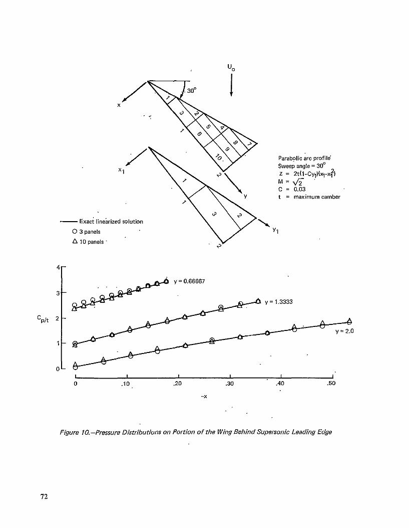
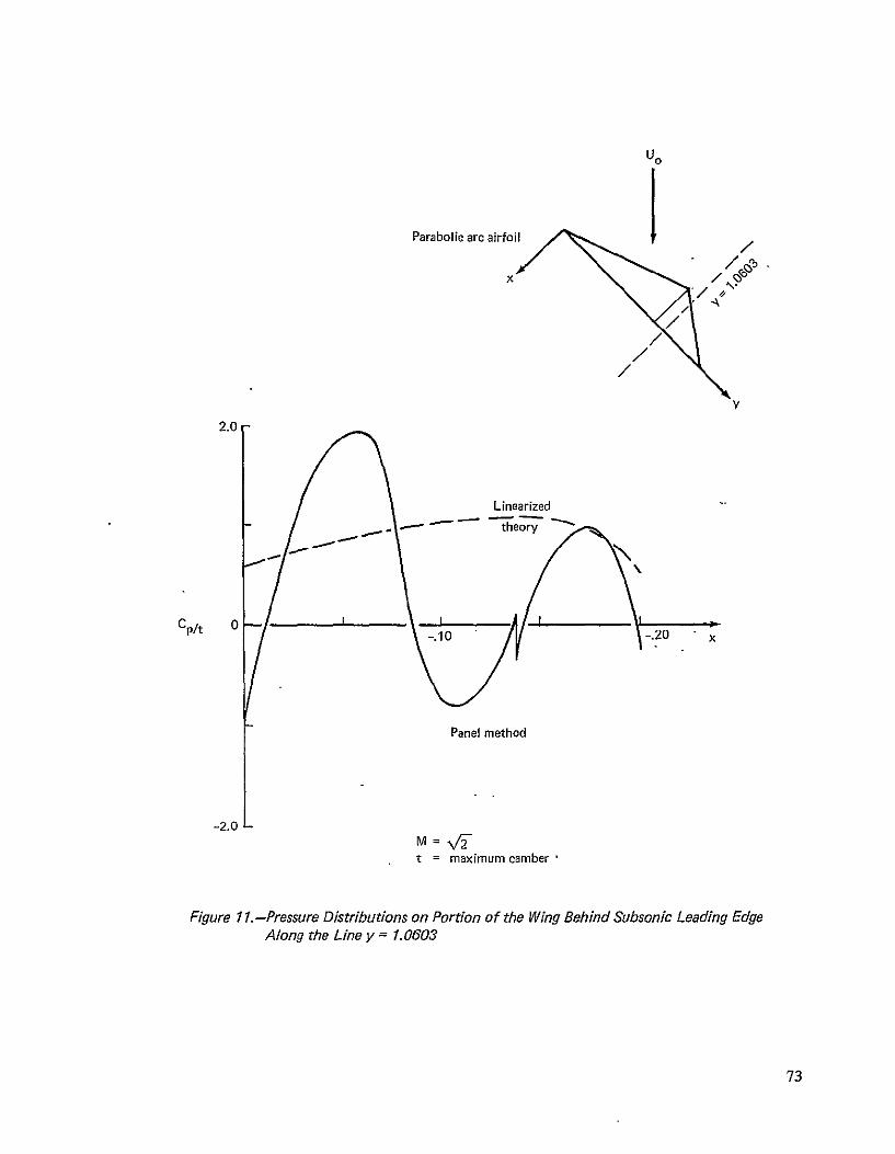
U0
Parabolic arc airfoil
y
20
Linearized theory
-2 x
Panel method
-20 M = NF2 t = maximum camber
Figure 11-Pressure Distributions on Portion of the Wing Behind Subsonic Leading Edge Along the Line y = 10603
73
U 0
A
Parabolic arc airfoil T
V
40
20
wt 0 -10-20 x
-20
Figure 12-Error in Downwash From Mach Line Doublet Panel Method Behind Subsonic Leading Edge Along the Line y = 10603
74
-1 F30
20 Upstream side
t -
-pDownstreashyside
10
X
Ctheory A
0 1 2
Distance along line L in units of panel width
Figure 13-Discontinuity in Pressure Coefficient Along Panel Edges of Mach Line Doublet Panels in the Region Behind Subsonic Leading Edge
75
- --
Line L4 Uo
xAx r45
A3
Parabolic arc profileFreestream mach number =Nr2 Sweep angle = 30
Doublet panel method Exact linearized solution
Cpt 2
1
0 1 2 3 4 5 WAY
Figure 14-Pressure Distribution Along Line L Downstream ofSpecial Mach Line With Flat Plate Solution Superimposed on Doublet Panel Solution
76
4 U- Line L
0 ~xI6x = -40O
Axi i-- I I bull
Parabolic arc profile
x Freestream mach number =V2
Sweep angle = 30Q
Doublbt panel method Exact linearized solution
1
0 1 2 3 4 5
yAy
Figure 15-Pressure Distribution Along Line L Downstream of Special Mach Line With FlatPlateSolution Superimposed on Doublet PanelSolution
77
$ Parabolic are profile x Freestream mach number=
Sweep angle = 300
Cpt -Doublet panel-method Exact linearized solution
0shy
-1 III I
0 3 4 5 yAY
Figure 16-Pressure Distribution Along Line L Downstream ofSpecial Mach Line With Flat Plate Solution Superimposed on Doublet Panel Solution
78
3 Uo Line L xz~x = 0
-- 1
4shy I
2 Parabolic arc profile x Freestream mach number =V2-
Sweep angle = 300
Cpt
N Doublet panel method
- 1I I i
0 1 2 3 4 5
yAy
Figure 17-Pressure Distribution Along Line L Downstream ofSpecial Mach Line With Flat Plate Solution Superimposed on Doublet Panel Solution
79
U0
Analysis only
0 Design only
x
gt Continuity of source
Downwash (or pressure) control point Pressure control point only
(design boundary conditions)
Y
Figure 18-Control Point Locations and Continuity Conditions for Source Mach Line Paneling
80
4
Solution with six panels
Exact linearized
solution
3shy
13 1 20shy
000--- shy
cpt 2
15
135--- shy
120 --- shy
105
U0
05
0 -1 - 2 x
Figure 19-Comparisonof Pressure DistributionFrom the Source Mach Line Panel Method With the Exact Solution From Linearized Theory for Wing With Parabolic Arc Profile
81
18
16 1 6 ~ ~Source solution
14- Prescribed slope
12 131 shy
8o35--- 20
M =Nf-
x I
0 - 1 - 2 x
Figure 20-Comparison ofSource Distribution With Wing Slopes
05
82
U0
Biconvec airfoil 20 6t Mach number =-shy
0 13
--x-23 y 15 0
10x
y
- Wing slope-dydx
A DownwashW t Thickness ratio
10 30
V
Figure 21-Comparison of Downwash From Supersonic Source Design Panel Method With Actual Wing Slopes
83
U0
51 ~i CYc
Cp
7Q 7
-b 4 r
II
~ampr
M-V2
M=V
y
Figure 22-Schematic Paneling on Wing Used to Test Mach Line Panel Methods
84
U0
Supersonic leading edge
u - a ffk
(c + dx)
+ (b+ dy ) + cy + dxy
e a + bx +cs 1 + dxs1
S
ar (b+ds) (x+62 s2 )
a + y
qOx +Oy =
a=
ax +a
=
0a=
xy
(b+dsl)e 2 s2
Figure 23-Region of Integration for Leadfng Edge Source Panel With the Zone of Dependence Terminated by a Subsonic Leading Edge
85
x
U0
or= dx~y = ds x G dS lX
Cr del ilY
ax+ OF 0o + O =delS1x o=dje S
Figure 24-Region of Integration for Interior Source Panel With the Zone of Dependence Terminated by a Subsonic Leading Edge
86
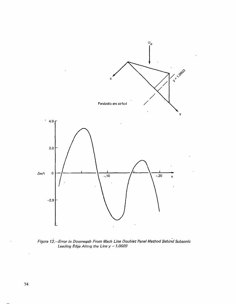
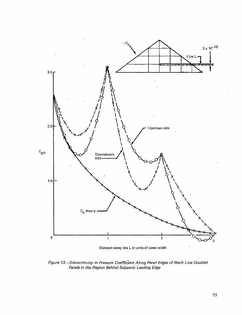
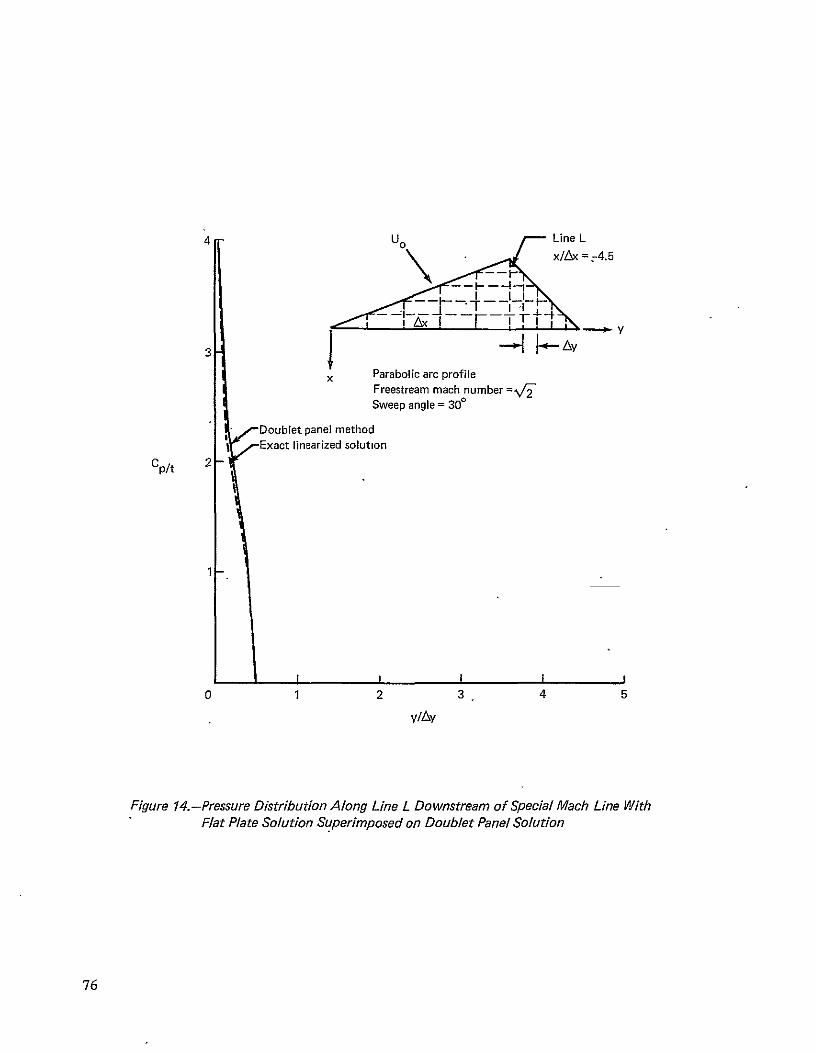
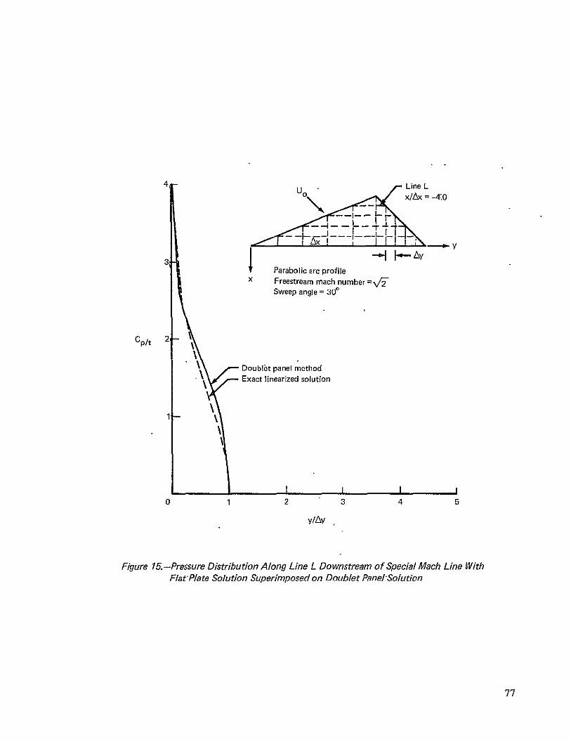
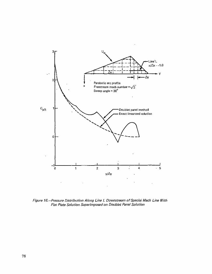
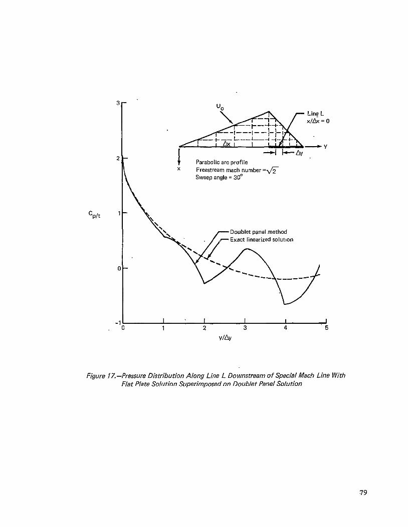
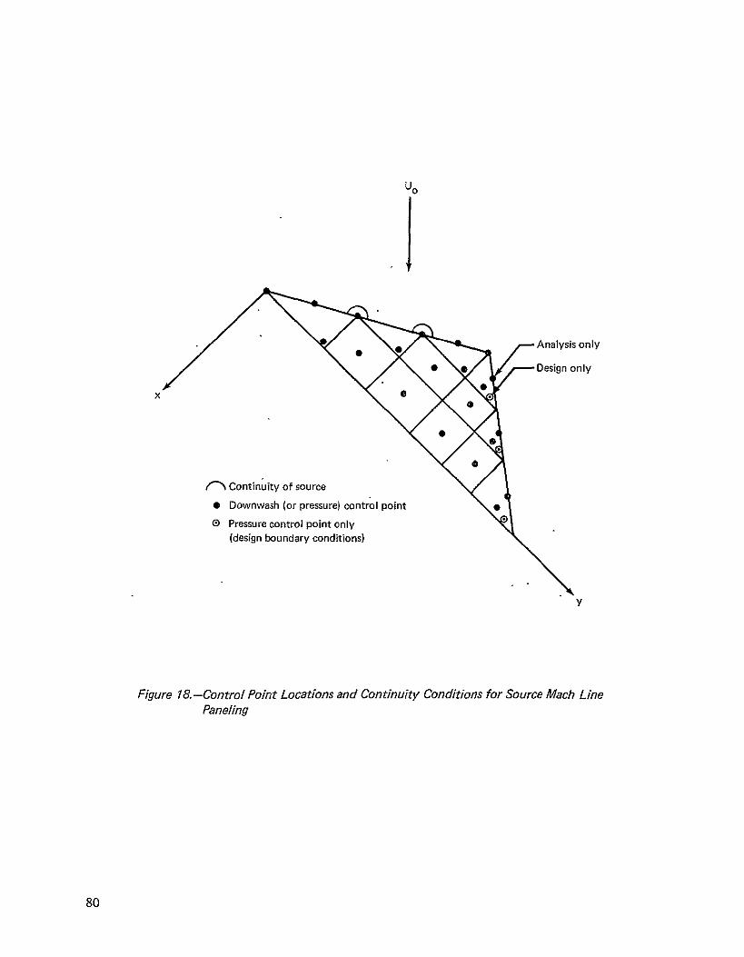
U0
Analysis only
0 Design only
x
gt Continuity of source
Downwash (or pressure) control point Pressure control point only
(design boundary conditions)
Y
Figure 18-Control Point Locations and Continuity Conditions for Source Mach Line Paneling
80
4
Solution with six panels
Exact linearized
solution
3shy
13 1 20shy
000--- shy
cpt 2
15
135--- shy
120 --- shy
105
U0
05
0 -1 - 2 x
Figure 19-Comparisonof Pressure DistributionFrom the Source Mach Line Panel Method With the Exact Solution From Linearized Theory for Wing With Parabolic Arc Profile
81
18
16 1 6 ~ ~Source solution
14- Prescribed slope
12 131 shy
8o35--- 20
M =Nf-
x I
0 - 1 - 2 x
Figure 20-Comparison ofSource Distribution With Wing Slopes
05
82
U0
Biconvec airfoil 20 6t Mach number =-shy
0 13
--x-23 y 15 0
10x
y
- Wing slope-dydx
A DownwashW t Thickness ratio
10 30
V
Figure 21-Comparison of Downwash From Supersonic Source Design Panel Method With Actual Wing Slopes
83
U0
51 ~i CYc
Cp
7Q 7
-b 4 r
II
~ampr
M-V2
M=V
y
Figure 22-Schematic Paneling on Wing Used to Test Mach Line Panel Methods
84
U0
Supersonic leading edge
u - a ffk
(c + dx)
+ (b+ dy ) + cy + dxy
e a + bx +cs 1 + dxs1
S
ar (b+ds) (x+62 s2 )
a + y
qOx +Oy =
a=
ax +a
=
0a=
xy
(b+dsl)e 2 s2
Figure 23-Region of Integration for Leadfng Edge Source Panel With the Zone of Dependence Terminated by a Subsonic Leading Edge
85
x
U0
or= dx~y = ds x G dS lX
Cr del ilY
ax+ OF 0o + O =delS1x o=dje S
Figure 24-Region of Integration for Interior Source Panel With the Zone of Dependence Terminated by a Subsonic Leading Edge
86
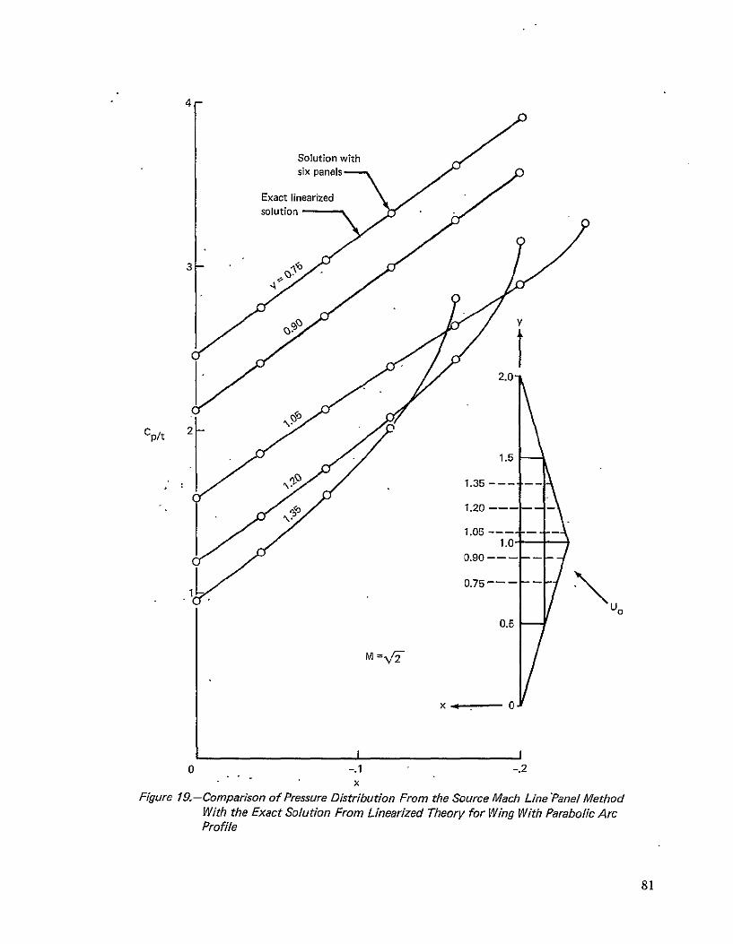
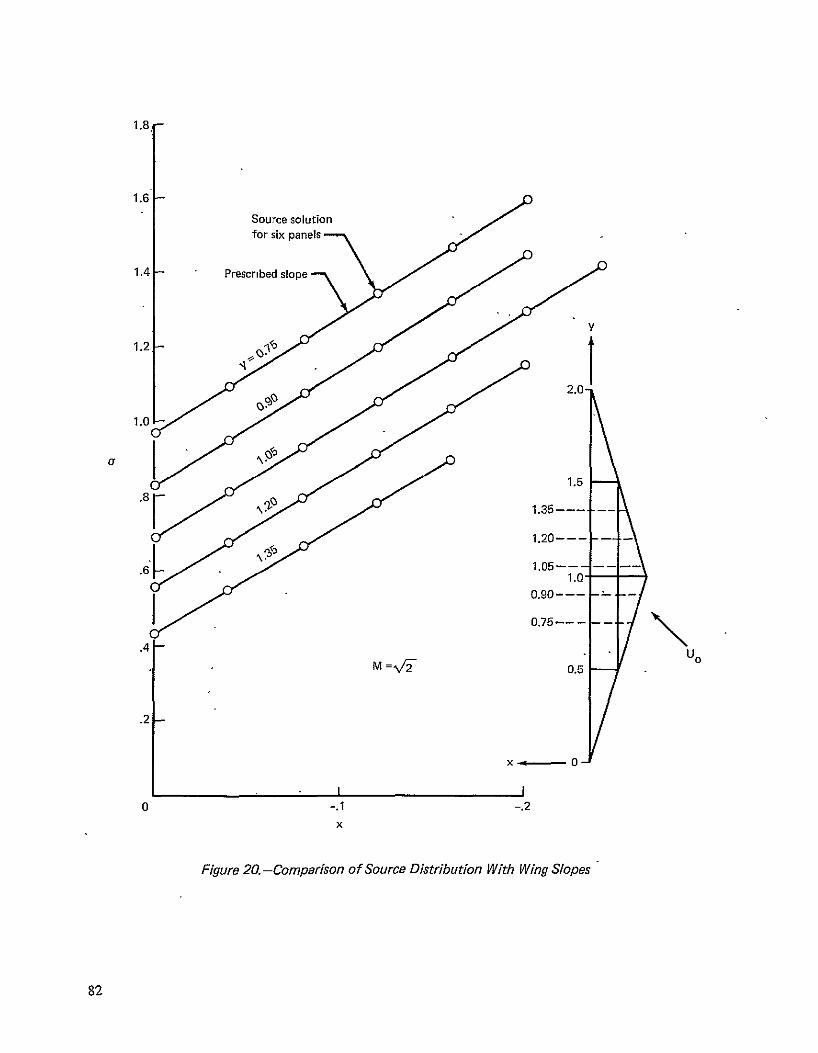
U0
Supersonic leading edge
u - a ffk
(c + dx)
+ (b+ dy ) + cy + dxy
e a + bx +cs 1 + dxs1
S
ar (b+ds) (x+62 s2 )
a + y
qOx +Oy =
a=
ax +a
=
0a=
xy
(b+dsl)e 2 s2
Figure 23-Region of Integration for Leadfng Edge Source Panel With the Zone of Dependence Terminated by a Subsonic Leading Edge
85
x
U0
or= dx~y = ds x G dS lX
Cr del ilY
ax+ OF 0o + O =delS1x o=dje S
Figure 24-Region of Integration for Interior Source Panel With the Zone of Dependence Terminated by a Subsonic Leading Edge
86
x
U0
or= dx~y = ds x G dS lX
Cr del ilY
ax+ OF 0o + O =delS1x o=dje S
Figure 24-Region of Integration for Interior Source Panel With the Zone of Dependence Terminated by a Subsonic Leading Edge
86


![Mach number P w,test [bar] P model [bar] 1.8 -0.45 -0.20 0 ...ae342/18/lab2/lab2data.pdf · Mach 2.0 Snapshot . Mach 1.8 Snapshot . Mach 2.3 Snapshot Mach 2.2 Snapshot . P w,test](https://img.pdfslide.us/doc/110x75/5fb4e5220b26be1bae0aea08/mach-number-p-wtest-bar-p-model-bar-18-045-020-0-ae34218lab2-.jpg)