1

A Lossless Compression Scheme for Bayer Color Filter

Array Images

King-Hong Chung and Yuk-Hee Chan1

Centre for Multimedia Signal Processing Department of Electronic and Information Engineering The Hong Kong Polytechnic University, Hong Kong

ABSTRACT

In most digital cameras, Bayer CFA images are captured and demosaicing is generally carried out before compression. Recently, it was found that compression-first schemes outperform the conventional demosaicing-first schemes in terms of output image quality. An efficient prediction-based lossless compression scheme for Bayer CFA images is proposed in this paper. It exploits a context matching technique to rank the neighboring pixels when predicting a pixel, an adaptive color difference estimation scheme to remove the color spectral redundancy when handling red and blue samples, and an adaptive codeword generation technique to adjust the divisor of Rice code for encoding the prediction residues. Simulation results show that the proposed compression scheme can achieve a better compression performance than conventional lossless CFA image coding schemes.

EDICS: COD-LSSI Lossless image coding; COD-OTHR Other

1 Corresponding author (Email: enyhchan@polyu.edu.hk)

2

1. INTRODUCTION

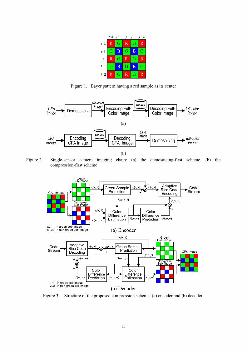
To reduce cost, most digital cameras use a single image sensor to capture color images. A Bayer color filter array (CFA) [1, 2], as shown in Figure 1, is usually coated over the sensor in these cameras to record only one of the three color components at each pixel location. The resultant image is referred to as a CFA image in this paper hereafter. In general, a CFA image is first interpolated via a demosaicing process [3-9] to form a full color image before being compressed for storage. Figure 2a shows the workflow of this imaging chain. Recently, some reports [10-14] indicated that such a demosaicing-first processing sequence was inefficient in a way that the demosaicing process always introduced some redundancy which should eventually be removed in the following compression step. As a result, an alternative processing sequence [10-13] which carries out compression before demosaicing as shown in Figure 2b has been proposed lately. Under this new strategy, digital cameras can have a simpler design and lower power consumption as computationally heavy processes like demosaicing can be carried out in an offline powerful personal computer. This motivates the demand of CFA image compression schemes. There are two categories of CFA image compression schemes: lossy and lossless. Lossy schemes compress a CFA image by discarding its visually redundant information. These schemes usually yield a higher compression ratio as compared with the lossless schemes. Schemes presented in [10-20] are some examples of this approach. In these schemes, different lossy compression techniques such as discrete cosine transform [15], vector quantization [16, 17] sub-band coding with symmetric short kernel filters [10], transform followed by JPEG or JPEG 2000 [12, 13, 18-20] and low-pass filtering followed by JPEG-LS or JPEG 2000 (lossless mode) [11] are used to reduce data redundancy. In some high-end photography applications such as commercial poster production, original CFA images are required for producing high quality full color images directly. In such cases, lossless compression of CFA images is necessary. Some lossless image compression schemes like JPEG-LS [21] and JPEG2000 [22] can be used to en-code a CFA image but only a fair performance can be attained. Recently, an advanced lossless CFA image compression scheme (LCMI) [23] was proposed. In this scheme, the mosaic data is de-correlated by the Mallat wavelet packet transform, and the coefficients are then compressed by Rice code. In this paper, a prediction-based lossless CFA compression scheme as shown in Figure 3 is proposed. It divides a CFA image into 2 sub-images: a green sub-image which contains all green samples of the CFA image and a non-green sub-image which holds the red and the blue samples. The green sub-image is coded first and the non-green sub-image follows based on the green sub-image as a reference. To reduce the spectral redundancy, the non-green sub-image is processed in the color difference domain whereas the green sub-image is processed in the intensity domain as a reference for the color difference content of the non-green sub-image. Both sub-images are processed in raster scan sequence with our proposed context matching based prediction technique to remove the spatial dependency. The prediction residue planes of the two sub-images are then entropy encoded sequentially with our proposed realization scheme of adaptive Rice code.

3

Experimental results show that the proposed compression scheme can effectively and efficiently reduce the redundancy in both spatial and color spectral domains. As compared with the existing lossless CFA image coding schemes such as [10-12], the proposed scheme provides the best compression performance in our simulation study. This paper is structured as follows. The proposed context matching based prediction technique is presented in Section 2. Section 3 shows how to estimate a missing green sample in the non-green sub-image of a CFA image for extracting the color difference information when compressing the non-green sub-image. In Section 4, how the prediction residue is adaptively encoded with Rice Code is provided. Section 5 demonstrates some simulation results and, finally, a conclusion is given in Section 6.

2. CONTEXT MATCHING BASED PREDICTION

The proposed prediction technique handles the green plane and the non-green plane separately in a raster scan manner. It weights the neighboring samples such that the one has higher context similarity to that of the current sample contributes more to the current prediction. Accordingly, this prediction technique is referred to as context matching based prediction (CMBP) in this paper. The green plane (green sub-image) is handled first as a CFA image contains double number of green samples to that of red/blue samples and the correlation among green samples can be exploited easily as compared with that among red or blue samples. Accordingly, the green plane can be used as a good reference to estimate the color difference of a red or blue sample when handling the non-green plane (non-green sub-image).

A. Prediction on the green plane

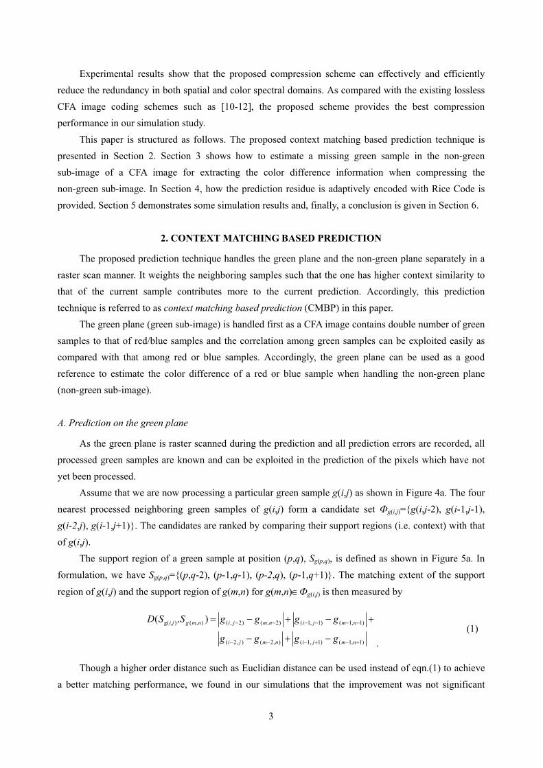
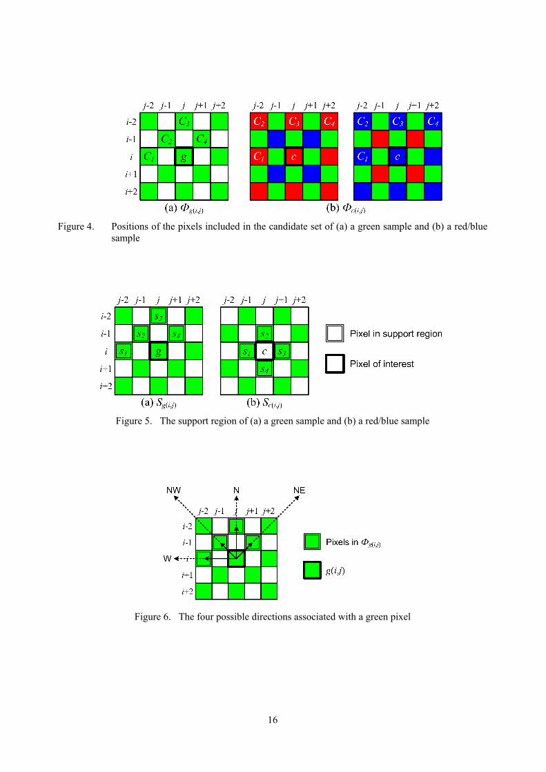
As the green plane is raster scanned during the prediction and all prediction errors are recorded, all processed green samples are known and can be exploited in the prediction of the pixels which have not yet been processed. Assume that we are now processing a particular green sample g(i,j) as shown in Figure 4a. The four nearest processed neighboring green samples of g(i,j) form a candidate set Фg(i,j)={g(i,j-2), g(i-1,j-1), g(i-2,j), g(i-1,j+1)}. The candidates are ranked by comparing their support regions (i.e. context) with that of g(i,j). The support region of a green sample at position (p,q), Sg(p,q), is defined as shown in Figure 5a. In formulation, we have Sg(p,q)={(p,q-2), (p-1,q-1), (p-2,q), (p-1,q+1)}. The matching extent of the support

region of g(i,j) and the support region of g(m,n) for g(m,n)∈Фg(i,j) is then measured by

)1,1()1,1(),2(),2(

)1,1()1,1()2,()2,(),()g(

)(

+−+−−−

−−−−−−

−+−

+−+−=

nmjinmji

nmjinmjinmgi,j

gggg

gggg,SSD

. (1)

Though a higher order distance such as Euclidian distance can be used instead of eqn.(1) to achieve a better matching performance, we found in our simulations that the improvement was not significant

4

enough to compensate for its high realization complexity.

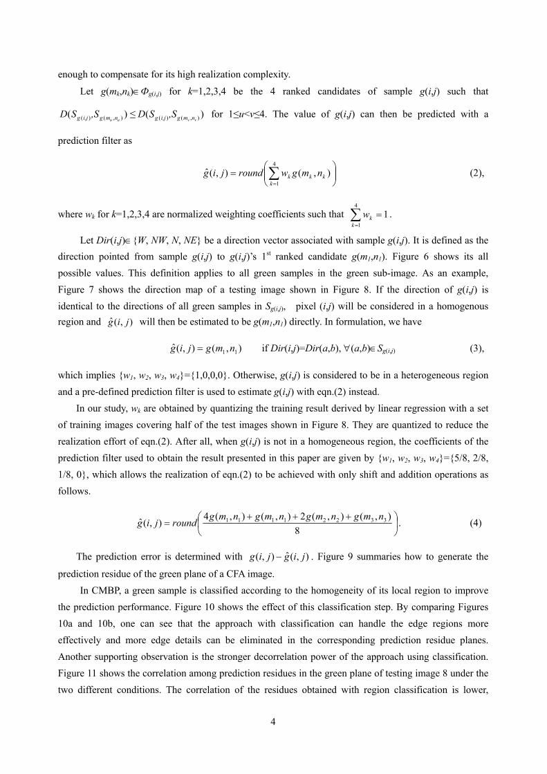
Let g(mk,nk)∈Фg(i,j) for k=1,2,3,4 be the 4 ranked candidates of sample g(i,j) such that

)( ),()( uu nmgi,jg ,SSD ≤ )( ),()( vv nmgi,jg ,SSD for 1≤u<v≤4. The value of g(i,j) can then be predicted with a

prediction filter as

= ∑

=

4

1),(),(ˆ

kkkk nmgwroundjig (2),

where wk for k=1,2,3,4 are normalized weighting coefficients such that 14

1=∑

=kkw .

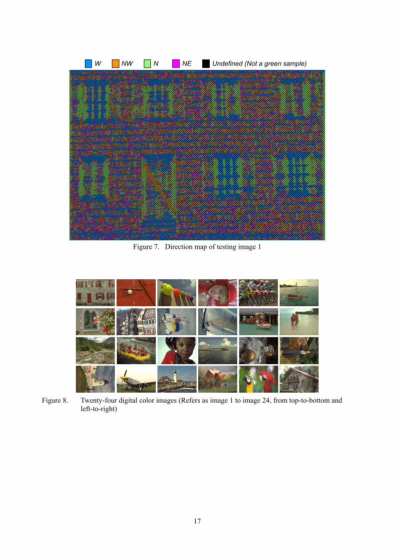
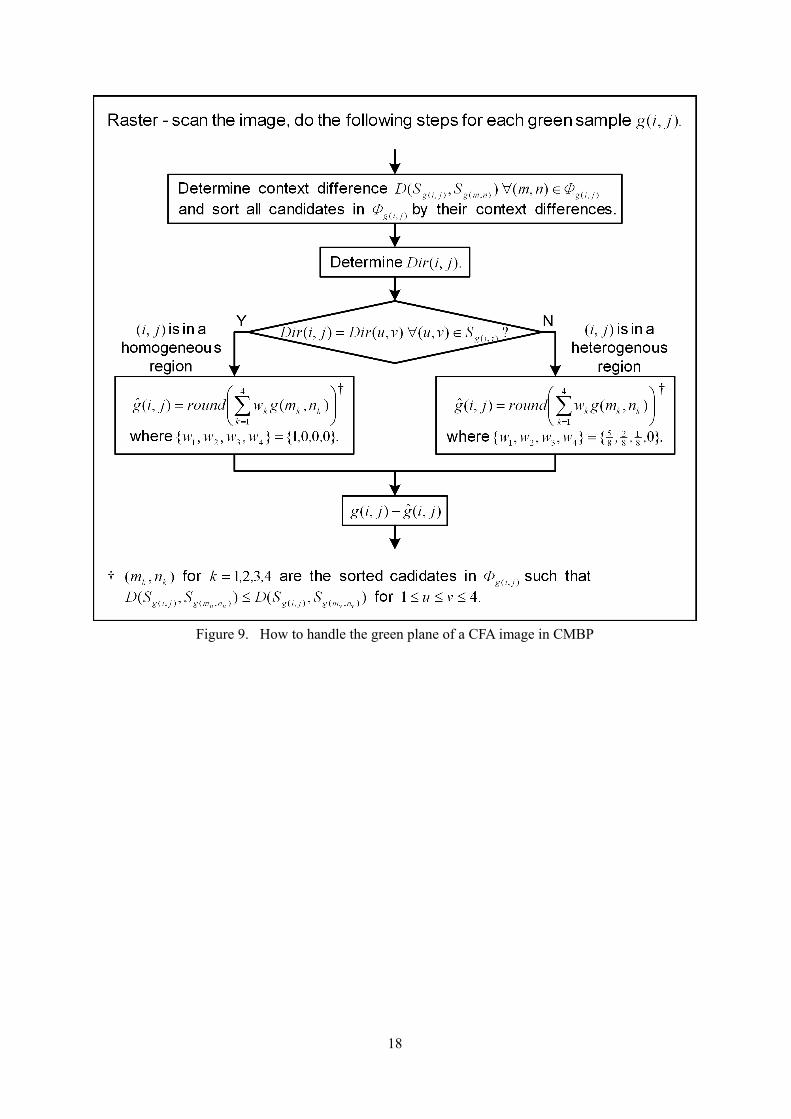
Let Dir(i,j)∈{W, NW, N, NE} be a direction vector associated with sample g(i,j). It is defined as the direction pointed from sample g(i,j) to g(i,j)’s 1st ranked candidate g(m1,n1). Figure 6 shows its all possible values. This definition applies to all green samples in the green sub-image. As an example, Figure 7 shows the direction map of a testing image shown in Figure 8. If the direction of g(i,j) is identical to the directions of all green samples in Sg(i,j), pixel (i,j) will be considered in a homogenous region and ),(ˆ jig will then be estimated to be g(m1,n1) directly. In formulation, we have

),(),(ˆ 11 nmgjig = if Dir(i,j)=Dir(a,b), ∀(a,b)∈Sg(i,j) (3),

which implies {w1, w2, w3, w4}={1,0,0,0}. Otherwise, g(i,j) is considered to be in a heterogeneous region and a pre-defined prediction filter is used to estimate g(i,j) with eqn.(2) instead.

In our study, wk are obtained by quantizing the training result derived by linear regression with a set of training images covering half of the test images shown in Figure 8. They are quantized to reduce the realization effort of eqn.(2). After all, when g(i,j) is not in a homogeneous region, the coefficients of the prediction filter used to obtain the result presented in this paper are given by {w1, w2, w3, w4}={5/8, 2/8, 1/8, 0}, which allows the realization of eqn.(2) to be achieved with only shift and addition operations as follows.

+++

=8

),(),(2),(),(4),(ˆ 33221111 nmgnmgnmgnmg

roundjig . (4)

The prediction error is determined with ),(ˆ),( jigjig − . Figure 9 summaries how to generate the

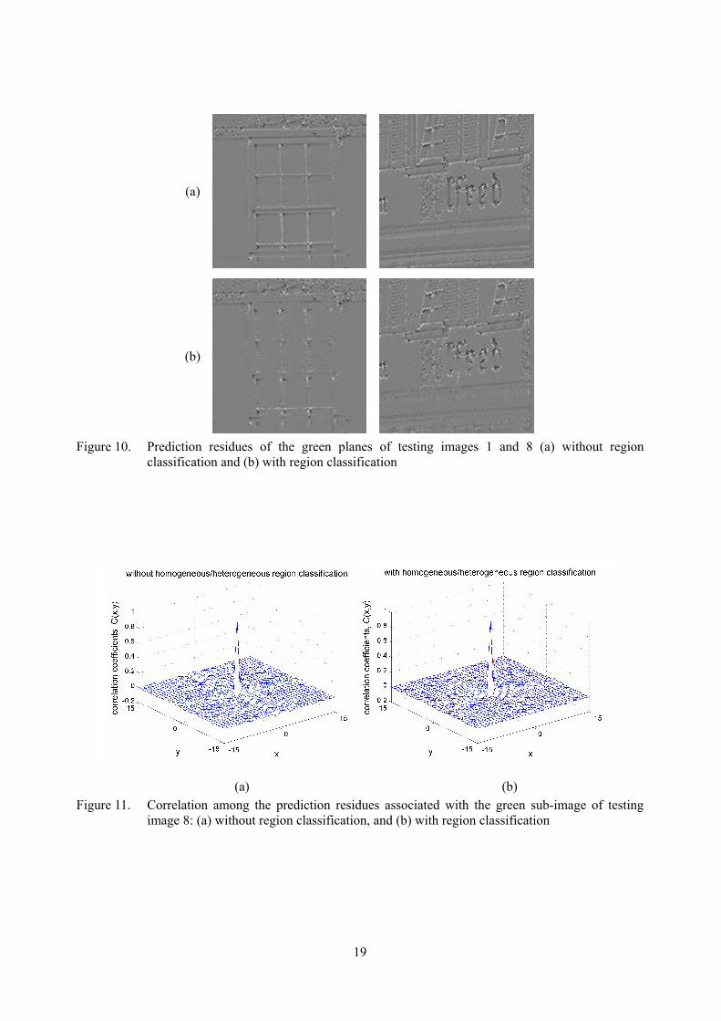
prediction residue of the green plane of a CFA image. In CMBP, a green sample is classified according to the homogeneity of its local region to improve the prediction performance. Figure 10 shows the effect of this classification step. By comparing Figures 10a and 10b, one can see that the approach with classification can handle the edge regions more effectively and more edge details can be eliminated in the corresponding prediction residue planes. Another supporting observation is the stronger decorrelation power of the approach using classification. Figure 11 shows the correlation among prediction residues in the green plane of testing image 8 under the two different conditions. The correlation of the residues obtained with region classification is lower,

5

which implies that the approach is more effective in data compression. Besides, the entropy of the prediction residues obtained with region classification is also lower. As far as testing image 8 is concerned, their zero-order entropy values are, respectively, 6.195 and 6.039 bpp. B. Prediction on the non-green plane

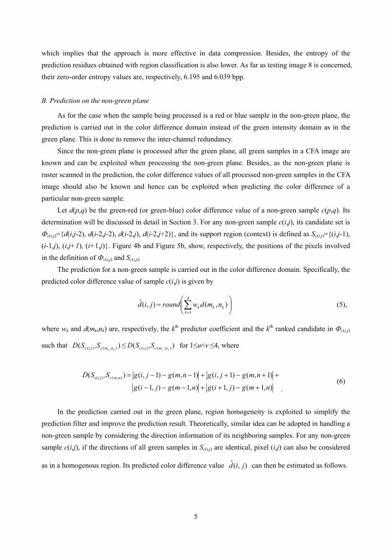
As for the case when the sample being processed is a red or blue sample in the non-green plane, the prediction is carried out in the color difference domain instead of the green intensity domain as in the green plane. This is done to remove the inter-channel redundancy. Since the non-green plane is processed after the green plane, all green samples in a CFA image are known and can be exploited when processing the non-green plane. Besides, as the non-green plane is raster scanned in the prediction, the color difference values of all processed non-green samples in the CFA image should also be known and hence can be exploited when predicting the color difference of a particular non-green sample. Let d(p,q) be the green-red (or green-blue) color difference value of a non-green sample c(p,q). Its determination will be discussed in detail in Section 3. For any non-green sample c(i,j), its candidate set is Фc(i,j)={d(i,j-2), d(i-2,j-2), d(i-2,j), d(i-2,j+2)}, and its support region (context) is defined as Sc(i,j)={(i,j-1), (i-1,j), (i,j+1), (i+1,j)}. Figure 4b and Figure 5b, show, respectively, the positions of the pixels involved in the definition of Фc(i,j) and Sc(i,j). The prediction for a non-green sample is carried out in the color difference domain. Specifically, the predicted color difference value of sample c(i,j) is given by

= ∑

=

),(),(ˆ4

1k

kkk nmdwroundjid (5),

where wk and d(mk,nk) are, respectively, the kth predictor coefficient and the kth ranked candidate in Фc(i,j)

such that )( ),()( uu nmci,jc ,SSD ≤ )( ),()( vv nmci,jc ,SSD for 1≤u<v ≤4, where

),1(),1(),1(),1(

)1,()1,()1,()1,()( ),()c(

nmgjignmgjig

nmgjignmgjig,SSD nmci,j

+−++−−−

++−++−−−=

. (6)

In the prediction carried out in the green plane, region homogeneity is exploited to simplify the prediction filter and improve the prediction result. Theoretically, similar idea can be adopted in handling a non-green sample by considering the direction information of its neighboring samples. For any non-green sample c(i,j), if the directions of all green samples in Sc(i,j) are identical, pixel (i,j) can also be considered

as in a homogenous region. Its predicted color difference value ),(ˆ jid can then be estimated as follows.

6

),(),(

),()2,2(),(),2(

),()2,2(),()2,(

),(ˆ jiSnm

NEnmDirifjidNnmDirifjid

NWnmDirifjidWnmDirifjid

jid c∈∀

=+−=−=−−=−

= (7)

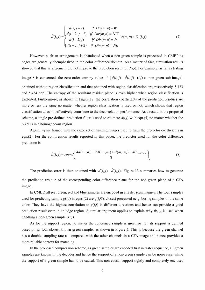
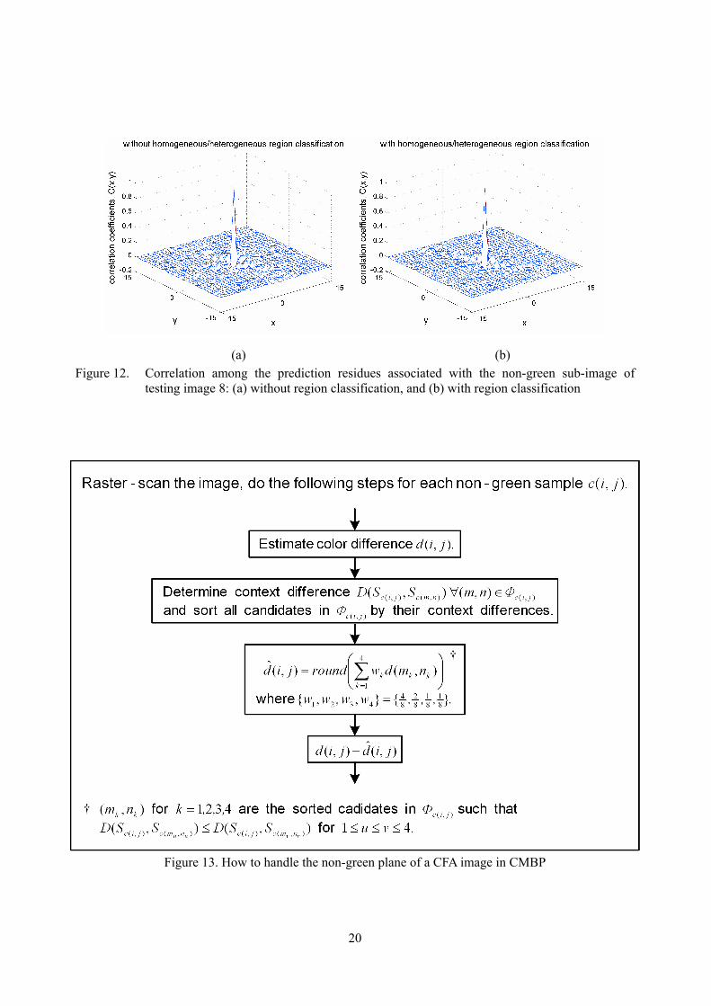
However, such an arrangement is abandoned when a non-green sample is processed in CMBP as edges are generally deemphasized in the color difference domain. As a matter of fact, simulation results showed that this arrangement did not improve the prediction result of d(i,j). For example, as far as testing

image 8 is concerned, the zero-order entropy value of { ),(ˆ),( jidjid − | (i,j) ∈ non-green sub-image}

obtained without region classification and that obtained with region classification are, respectively, 5.423 and 5.434 bpp. The entropy of the resultant residue plane is even higher when region classification is exploited. Furthermore, as shown in Figure 12, the correlation coefficients of the prediction residues are more or less the same no matter whether region classification is used or not, which shows that region classification does not effectively contribute to the decorrelation performance. As a result, in the proposed scheme, a single pre-defined prediction filter is used to estimate d(i,j) with eqn.(5) no matter whether the pixel is in a homogeneous region. Again, wk are trained with the same set of training images used to train the predictor coefficients in eqn.(2). For the compression results reported in this paper, the predictor used for the color difference prediction is

+++

=8

),(),(),(2),(4),(ˆ 44332211 nmdnmdnmdnmdroundjid. (8)

The prediction error is then obtained with ),(ˆ),( jidjid − . Figure 13 summaries how to generate

the prediction residue of the corresponding color-difference plane for the non-green plane of a CFA image. In CMBP, all real green, red and blue samples are encoded in a raster scan manner. The four samples used for predicting sample g(i,j) in eqns.(2) are g(i,j)’s closest processed neighboring samples of the same color. They have the highest correlation to g(i,j) in different directions and hence can provide a good prediction result even in an edge region. A similar argument applies to explain why Фc(i,j) is used when handling a non-green sample c(i,j). As for the support region, no matter the concerned sample is green or not, its support is defined based on its four closest known green samples as shown in Figure 5. This is because the green channel has a double sampling rate as compared with the other channels in a CFA image and hence provides a more reliable context for matching. In the proposed compression scheme, as green samples are encoded first in raster sequence, all green samples are known in the decoder and hence the support of a non-green sample can be non-causal while the support of a green sample has to be causal. This non-causal support tightly and completely encloses

7

the sample of interest. It models image features such as intensity gradient, edge orientation and textures better such that more accurate support matching can be achieved.

3. ADAPTIVE COLOR DIFFERENCE ESTIMATION

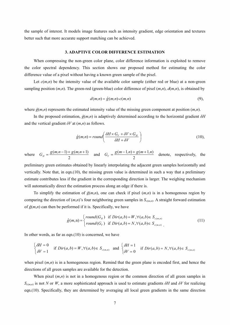
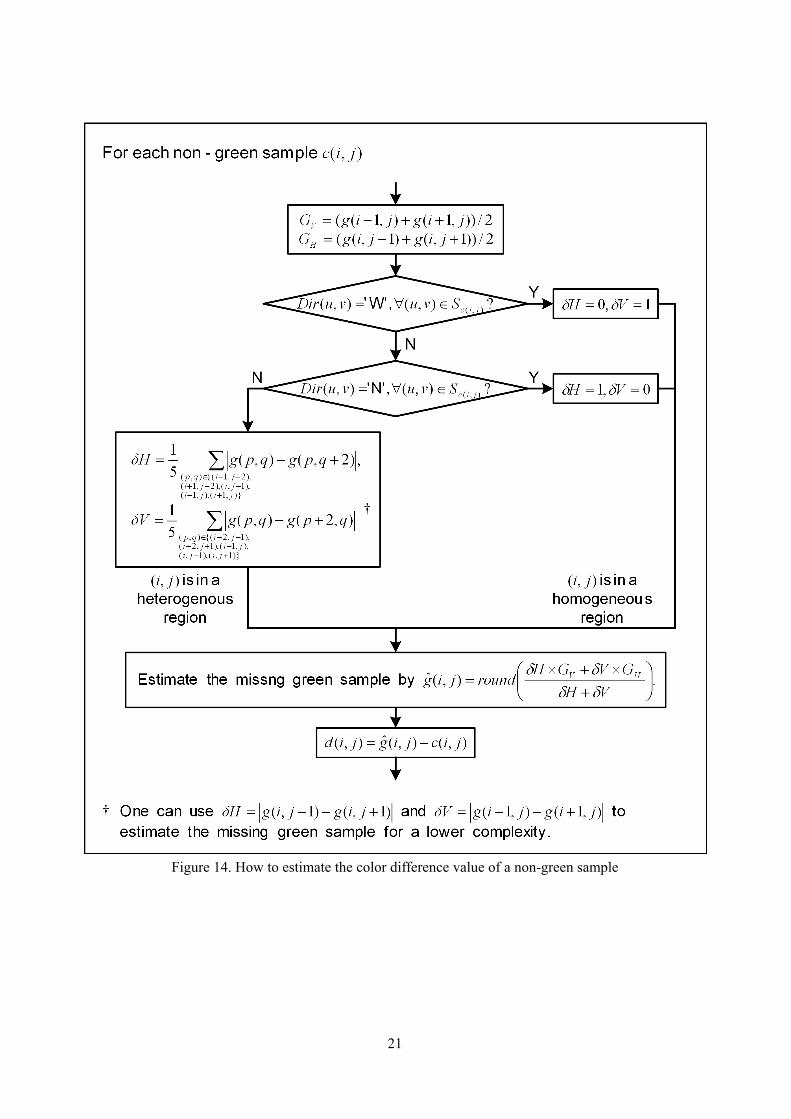
When compressing the non-green color plane, color difference information is exploited to remove the color spectral dependency. This section shows our proposed method for estimating the color difference value of a pixel without having a known green sample of the pixel. Let c(m,n) be the intensity value of the available color sample (either red or blue) at a non-green sampling position (m,n). The green-red (green-blue) color difference of pixel (m,n), d(m,n), is obtained by

)()(ˆ)( m,n-cm,ngm,nd = (9),

where ĝ(m,n) represents the estimated intensity value of the missing green component at position (m,n). In the proposed estimation, ĝ(m,n) is adaptively determined according to the horizontal gradient δH and the vertical gradient δV at (m,n) as follows.

+×+×

=δVδH

GδVGδHroundm,ng HV)(ˆ (10),

where 2

)1()1( ++−=

m,ngm,ngGH and 2

)1()1( ,nmg,nmgGV++−

= denote, respectively, the

preliminary green estimates obtained by linearly interpolating the adjacent green samples horizontally and vertically. Note that, in eqn.(10), the missing green value is determined in such a way that a preliminary estimate contributes less if the gradient in the corresponding direction is larger. The weighing mechanism will automatically direct the estimation process along an edge if there is. To simplify the estimation of ĝ(m,n), one can check if pixel (m,n) is in a homogenous region by comparing the direction of (m,n)’s four neighboring green samples in Sc(m,n). A straight forward estimation of ĝ(m,n) can then be performed if it is. Specifically, we have

∈∀=∈∀=

=),(

),(

),(,),( if )(),(,),( if )(

n),(ˆnmcV

nmcH

SbaNbaDirGroundSbaWbaDirGround

mg. (11)

In other words, as far as eqn.(10) is concerned, we have

∈∀===

),(),(,),( if10

nmcSbaWbaDirVHδδ

and

∈∀===

),(),(,),( if01

nmcSbaNbaDirVHδδ

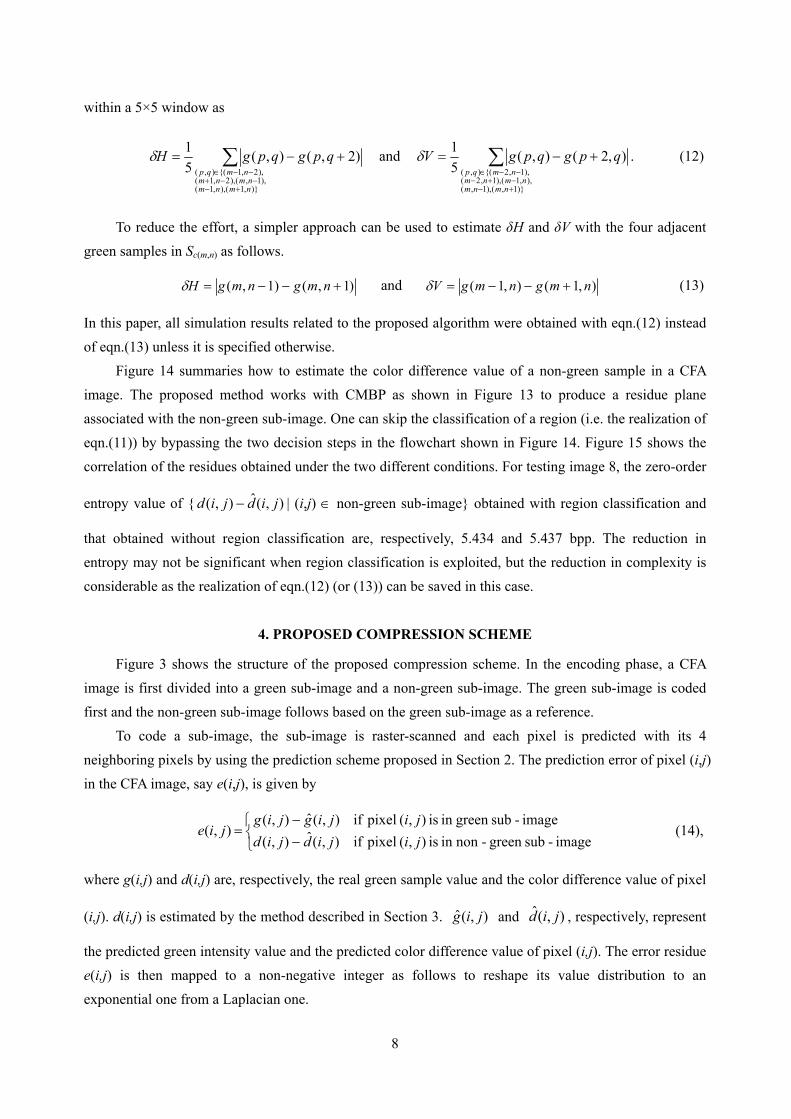
when pixel (m,n) is in a homogenous region. Remind that the green plane is encoded first, and hence the directions of all green samples are available for the detection. When pixel (m,n) is not in a homogenous region or the common direction of all green samples in Sc(m,n) is not N or W, a more sophisticated approach is used to estimate gradients δH and δV for realizing eqn.(10). Specifically, they are determined by averaging all local green gradients in the same direction

8

within a 5×5 window as

∑+−

−−+−−∈

+−=

)},1(),,1(),1,(),2,1(

),2,1{(),(2),(),(

51

nmnmnmnm

nmqpqpgqpgHδ and ∑

+−−+−−−∈

+−=

)}1,(),1,(),,1(),1,2(

),1,2{(),(

),2(),(51

nmnmnmnm

nmqp

qpgqpgVδ . (12)

To reduce the effort, a simpler approach can be used to estimate δH and δV with the four adjacent green samples in Sc(m,n) as follows.

)1,(1),( +−−= nmgnmgHδ and ),1(),1( nmgnmgV +−−=δ (13)

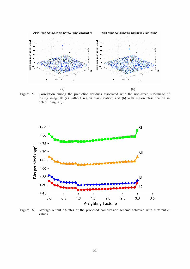
In this paper, all simulation results related to the proposed algorithm were obtained with eqn.(12) instead of eqn.(13) unless it is specified otherwise. Figure 14 summaries how to estimate the color difference value of a non-green sample in a CFA image. The proposed method works with CMBP as shown in Figure 13 to produce a residue plane associated with the non-green sub-image. One can skip the classification of a region (i.e. the realization of eqn.(11)) by bypassing the two decision steps in the flowchart shown in Figure 14. Figure 15 shows the correlation of the residues obtained under the two different conditions. For testing image 8, the zero-order

entropy value of { ),(ˆ),( jidjid − | (i,j) ∈ non-green sub-image} obtained with region classification and

that obtained without region classification are, respectively, 5.434 and 5.437 bpp. The reduction in entropy may not be significant when region classification is exploited, but the reduction in complexity is considerable as the realization of eqn.(12) (or (13)) can be saved in this case.

4. PROPOSED COMPRESSION SCHEME

Figure 3 shows the structure of the proposed compression scheme. In the encoding phase, a CFA image is first divided into a green sub-image and a non-green sub-image. The green sub-image is coded first and the non-green sub-image follows based on the green sub-image as a reference. To code a sub-image, the sub-image is raster-scanned and each pixel is predicted with its 4 neighboring pixels by using the prediction scheme proposed in Section 2. The prediction error of pixel (i,j) in the CFA image, say e(i,j), is given by

−−

=image-subgreen -nonin is ),( pixel if),(ˆ),(

image-subgreen in is ),( pixel if),(ˆ),(),(

jijidjidjijigjig

jie (14),

where g(i,j) and d(i,j) are, respectively, the real green sample value and the color difference value of pixel

(i,j). d(i,j) is estimated by the method described in Section 3. ),(ˆ jig and ),(ˆ jid , respectively, represent

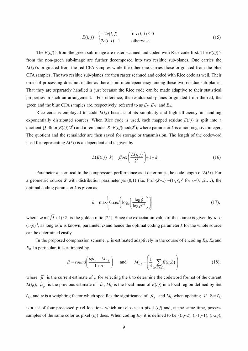
the predicted green intensity value and the predicted color difference value of pixel (i,j). The error residue e(i,j) is then mapped to a non-negative integer as follows to reshape its value distribution to an exponential one from a Laplacian one.

9

−≤−

=otherwise1 ),(2

0),( if),(2),(

jiejiejie

jiE (15)

The E(i,j)’s from the green sub-image are raster scanned and coded with Rice code first. The E(i,j)’s from the non-green sub-image are further decomposed into two residue sub-planes. One carries the E(i,j)’s originated from the red CFA samples while the other one carries those originated from the blue CFA samples. The two residue sub-planes are then raster scanned and coded with Rice code as well. Their order of processing does not matter as there is no interdependency among these two residue sub-planes. That they are separately handled is just because the Rice code can be made adaptive to their statistical properties in such an arrangement. For reference, the residue sub-planes originated from the red, the green and the blue CFA samples are, respectively, referred to as ER, EG and EB. Rice code is employed to code E(i,j) because of its simplicity and high efficiency in handling exponentially distributed sources. When Rice code is used, each mapped residue E(i,j) is split into a quotient Q=floor(E(i,j)/2k) and a remainder R=E(i,j)mod(2k), where parameter k is a non-negative integer. The quotient and the remainder are then saved for storage or transmission. The length of the codeword used for representing E(i,j) is k–dependent and is given by

kjiEfloorki,jEL k ++

= 1

2),()|)(( . (16)

Parameter k is critical to the compression performance as it determines the code length of E(i,j). For

a geometric source S with distribution parameter ρ∈(0,1) (i.e. Prob(S=s) =(1-ρ)ρs for s=0,1,2,…), the optimal coding parameter k is given as

= −12 log

loglog,0maxρφceilk (17),

where 2/)15( +=φ is the golden ratio [24]. Since the expectation value of the source is given by µ=ρ

(1-ρ)-1, as long as µ is known, parameter ρ and hence the optimal coding parameter k for the whole source can be determined easily. In the proposed compression scheme, µ is estimated adaptively in the course of encoding ER, EG and EB. In particular, it is estimated by

+

+=

αµα

µ1

~~ , jip M

round and

= ∑

∈ jibaji baEM

,),(, ),(

41

ζ

(18),

where µ~ is the current estimate of µ for selecting the k to determine the codeword format of the current E(i,j), pµ

~ is the previous estimate of µ~ , Mi,j is the local mean of E(i,j) in a local region defined by Set

ζi,j, and α is a weighting factor which specifies the significance of pµ~ and Mi,j when updating µ~ . Set ζi,j

is a set of four processed pixel locations which are closest to pixel (i,j) and, at the same time, possess samples of the same color as pixel (i,j) does. When coding EG, it is defined to be {(i,j-2), (i-1,j-1), (i-2,j),

10

(i-1,j+1)}. For coding ER and EB, Set ζi,j is defined to be {(i,j-2), (i-2,j-2), (i-2,j), (i-2,j+2)}. µ~ is updated for each E(i,j). The initial value of pµ

~ is 0 for all residue sub-planes.

Experimental results showed that α=1 can provide a good compression performance. Figure 16 shows how parameter α affects the final compression ratio of the proposed compression scheme. Curve R, G and B respectively show the cases when coding ER, EG and EB. The curve marked with ‘All’ shows the

overall performance when all residue sub-planes are compressed with a common α value. The decoding process is just the reverse process of encoding. The green sub-image is decoded first and then the non-green sub-image is decoded with the decoded green sub-image as a reference. The original CFA image is then reconstructed by combining the two sub-images.

5. COMPRESSION PERFORMANCE

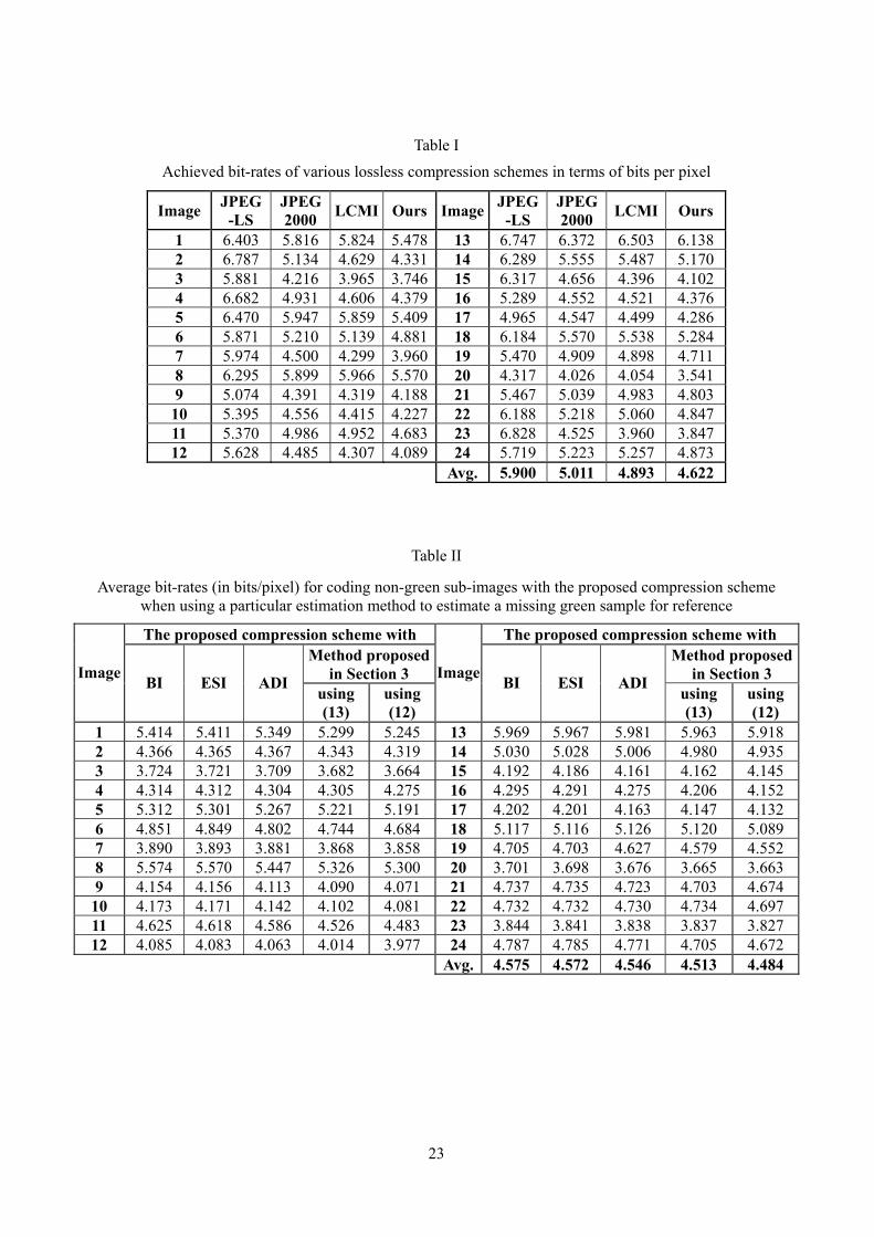
Simulations were carried out to evaluate the performance of the proposed compression scheme. Twenty-four 24-bit color images of size 512×768 each as shown in Figure 8 were sub-sampled according to the Bayer pattern to form a set of 8-bit testing CFA images. They were then directly coded by the proposed compression scheme for evaluation. Some representative lossless compression schemes such as JPEG-LS [21], JPEG 2000 (lossless mode) [22] and LCMI [23] were also evaluated for comparison. Table I lists the average output bit-rates of the CFA images achieved by various compression schemes in terms of bits per pixel (bpp). It clearly shows that the proposed scheme outperforms all other evaluated schemes in all testing images. Especially for the images which contain many edges and fine textures such as images 1, 5, 8, 13, 20 and 24, the bit-rates achieved by the proposed scheme are at least 0.34bpp lower than the corresponding bit-rates achieved by LCMI, the scheme offers the second best compression performance. These results demonstrate that the proposed compression scheme is robust to remove the CFA data dependency even though the image contains complicated structures. On average, the proposed scheme yields a bit-rate as low as 4.622bpp. It is, respectively, around 78.3%, 92.1% and 94.5% of those achieved by JPEG-LS, JPEG2000 and LCMI. In the proposed compression scheme, the non-green sub-image is processed in the color difference domain. Accordingly, the missing green samples in the sub-image have to be estimated for extracting the color difference information of the non-green sub-image. An estimation method for estimating the missing green samples and its simplified version (using eqn.(13) instead of eqn.(12) to estimate δH and δV), are proposed in Section 3. Obviously, one can make use of some other estimation methods such as bilinear interpolation [9] (BI), edge sensing interpolation [8] (ESI) and adaptive directional interpolation [4] (ADI) to achieve the same objective. For comparison, a simulation was carried out to evaluate the performance of these methods when they were used to compress a non-green sub-image with the proposed compression scheme. In this study, only the non-green sub-images are involved as the compression of green sub-images does not involve the estimation of missing green components. In the realization of BI, a missing green sample is estimated by rounding the average value of its four surrounding known green samples. For ESI, the four surrounding known green samples are weighted before averaging. The weights are determined according to the

11

gradients among the four known green samples [8]. ADI is a directional linear-based interpolation method in which the interpolation direction is determined by comparing the horizontal and vertical green gradients to a pre-defined threshold [4]. The threshold value was set to be 30 in our simulation as it provided the best compression result for the training set. Table II reveals the average bit rates of the outputs achieved by the proposed compression scheme when different methods were used to estimate the missing green samples in the non-green sub-images. It shows that the adaptive estimation methods proposed in Section 3 are superior to the other evaluated estimation methods. On average, the best proposed estimation method achieves a bit-rate of 4.484 bpp which is around 0.1 bpp lower than that achieved by BI.

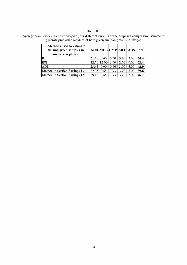
While Table II reports the compression performance of the proposed compression scheme and its various variants, Table III lists their complexity cost paid for producing all prediction residues of both green and non-green planes. It is measured in terms of the average number of operations required per pixel in our simulations. Operations including addition (ADD), multiplication (MUL), bit-shift (SHT), comparison (CMP) and taking absolute value (ABS) are all taken into account.

The proposed compression scheme is composed of four functional components. A study was carried out to evaluate the contribution of each component to the overall performance of the scheme. The same set of 24 testing CFA images were used again in the evaluation. In particular, when the prediction

components are switched off (i.e. ),(ˆ jig = ),(ˆ jid =0 in Figure 3a), the zero-order entropy values of

{e(i,j)|(i,j) ∈ green subimage} and {e(i,j)|(i,j) ∈ non-green subimage} are, respectively, 7.114 and 6.295 bpp on average, which are around 40.3% and 34.2% higher than the case when the prediction components are on. As for the component of color difference estimation, the proposed adaptive color difference estimation scheme provided a non-green residue plane of zero-order entropy 4.690 bpp on average, which is 0.114 bpp lower than that provided by using bilinear interpolation instead. To show the contribution of the proposed adaptive Rice code encoding scheme, we encoded E(i,j) with the conventional Rice code instead of the proposed one for comparison. In its realization, the coding parameter k for coding a sub-image is fixed and determined with eqn.(17). The parameter µ is estimated to be the mean of E(i,j) in the sub-image. After all, it achieved an average bit-rate of 5.084 bpp, which is 0.462 bpp higher than that achieved by using the proposed adaptive Rice code encoding scheme. When the proposed compression scheme (with eqn.(12)) was implemented in software with C++ programming language, the average execution time to compress a 512×768 CFA image on a 2.8GHz Pentium 4 PC with 512MB RAM is around 0.11s.

6. CONCLUSIONS

In this paper, a lossless compression scheme for Bayer images is proposed. This scheme separates a CFA image into a green sub-image and a non-green sub-image and then encodes them separately with predictive coding. The prediction is carried out in the intensity domain for the green sub-image while it is carried out in the color difference domain for the non-green sub-image. In both cases, a context matching

12

technique is used to rank the neighboring pixels of a pixel for predicting the existing sample value of the pixel. The prediction residues originated from the red, the green and the blue samples of the CFA images are then separately encoded. The value distribution of the prediction residue can be modeled as an exponential distribution, and hence Rice code is used to encode the residues. We assume the prediction residue is a local variable and estimate the mean of its value distribution adaptively. The divisor used to generate the Rice code is then adjusted accordingly so as to improve the efficiency of Rice code.

Experimental results show that the proposed compression scheme can efficiently and effectively decorrelate the data dependency in both spatial and color spectral domains. Consequently, it provides the best average compression ratio as compared with the latest lossless Bayer image compression schemes.

ACKNOWLEDGEMENT

This work was supported by a grant from the Research Grants Council of the Hong Kong Special Administrative Region, China (PolyU 5205/04E) and a grant from The Hong Kong Polytechnic University (G-U413).

REFERENCES

[1] B. E. Bayer, Color imaging array, U.S. 3 971 065, to Eastman Kodak Company (Rochester, NY), 1976.

[2] R. Lukac, and K. N. Plataniotis, “Color filter arrays: design and performance analysis,” Consumer Electronics, IEEE Transactions on, vol. 51, no. 4, pp. 1260-1267, 2005.

[3] J. F. Hamilton, and J. E. Adams, Adaptive color plan interpolation in single sensor color electronic camera, U.S. 5 629 734, to Eastman Kodak Company (Rochester, NY), 1997.

[4] R. H. Hibbard, Apparatus and method for adaptively interpolating a full color image utilizing luminance gradients, U.S. 5 382 976, to Eastman Kodak Company (Rochester, NY), 1995.

[5] B. K. Gunturk, Y. Altunbasak, and R. M. Mersereau, “Color plane interpolation using alternating projections,” IEEE Transactions on Image Processing, vol. 11, no. 9, pp. 997-1013, Sep, 2002.

[6] X. L. Wu, and N. Zhang, “Primary-consistent soft-decision color demosaicking for digital cameras - (Patent pending),” IEEE Transactions on Image Processing, vol. 13, no. 9, pp. 1263-1274, Sep, 2004.

[7] K. H. Chung, and Y. H. Chan, “Color demosaicing using variance of color differences,” IEEE Transactions on Image Processing, vol. 15, no. 10, pp. 2944-2955, Oct, 2006.

[8] R. Lukac, and K. N. Plataniotis, “Data adaptive filters for demosaicking: A framework,” IEEE Transactions on Consumer Electronics, vol. 51, no. 2, pp. 560-570, May, 2005.

[9] T. Sakamoto, C. Nakanishi, and T. Hase, “Software pixel interpolation for digital still cameras suitable for a 32-bit MCU,” IEEE Transactions on Consumer Electronics, vol. 44, no. 4, pp. 1342-1352, Nov, 1998.

[10] T. Toi, and M. Ohta, “A subband coding technique for image compression in single CCD cameras

13

with Bayer color filter arrays,” IEEE Transactions on Consumer Electronics, vol. 45, no. 1, pp. 176-180, Feb, 1999.

[11] X. Xie, G. Li, Z. Wang et al., “A novel method of lossy image compression for digital image sensors with Bayer color filter arrays,” in IEEE International Symposium on Circuits and Systems (ISCAS'05), Kobe, Japan, 2005, pp. 4995-4998.

[12] S. Y. Lee, and A. Ortega, “A novel approach of image compression in digital cameras with a Bayer color filter array,” in IEEE International Conference on Image Processing (ICIP'01), Thessaloniki, Greece, 2001, pp. 482-485.

[13] C. C. Koh, J. Mukherjee, and S. K. Mitra, “New efficient methods of image compression in digital cameras with color filter array,” IEEE Transactions on Consumer Electronics, vol. 49, no. 4, pp. 1448-1456, Nov, 2003.

[14] N. X. Lian, L. L. Chang, V. Zagorodnov et al., “Reversing demosaicking and compression in color filter array image processing: Performance analysis and modeling,” IEEE Transactions on Image Processing, vol. 15, no. 11, pp. 3261-3278, Nov, 2006.

[15] Y. T. Tsai, “Color image compression for single-chip cameras,” IEEE Transactions on Electron Devices, vol. 38, no. 5, pp. 1226-1232, May, 1991.

[16] A. Bruna, F. Vella, A. Buemi et al., "Predictive differential modulation for CFA compression," Proceedings of the 6th Nordic Signal Processing Symposium - NORSIG 2004, pp. 101-104, 2004.

[17] S. Battiato, A. Bruna, A. Buemi et al., “Coding techniques for CFA data images,” in International Conference on Image Analysis and Processing (ICIAP'03), Mantova, Italy, 2003, pp. 418-423.

[18] A. Bazhyna, A. Gotchev, and K. Egiazarian, "Near-lossless compression algorithm for Bayer pattern color filter arrays," Proceeding of SPIE - the International Society for Optical Engineering, vol. 5678, pp. 98-209, 2005.

[19] B. Parrein, M. Tarin, and P. Horain, “Demosaicking and JPEG2000 compression of microscopy images,” in IEEE International Conference on Image Processing (ICIP'04), Singapore, 2004, pp. 521-524.

[20] R. Lukac, and K. N. Plataniotis, “Single-sensor camera image compression,” IEEE Transactions on Consumer Electronics, vol. 52, no. 2, pp. 299-307, 2006.

[21] Information Technology - Lossless and Near-Lossless Compression of Continuous-Tone Still Images (JPEG-LS), ISO/IEC Standard 14495-1, 1999.

[22] Information technology - JPEG 2000 image coding system - Part 1: Core coding system, INCITS/ISO/IEC Standard 15444-1, 2000.

[23] N. Zhang, and X. L. Wu, “Lossless compression of color mosaic images,” IEEE Transactions on Image Processing, vol. 15, no. 6, pp. 1379-1388, 2006.

[24] A. Said, On the determination of optimal parameterized prefix codes for adaptive entropy coding, Technical Report HPL-2006-74, HP Laboratories Palo Alto, 2006.

14

Figure caption Figure 1. Bayer pattern having a red sample as its center Figure 2. Single-sensor camera imaging chain: (a) the demosaicing- first scheme, (b) the

compression-first scheme Figure 3. Structure of the proposed compression scheme: (a) encoder and (b) decoder Figure 4. Positions of the pixels included in the candidate set of (a) a green sample and (b) a red/blue

sample Figure 5. The support region of (a) a green sample and (b) a red/blue sample Figure 6. The four possible directions associated with a green pixel Figure 7. Direction map of testing image 1 Figure 8. Twenty-four digital color images (Refers as image 1 to image 24, from top-to-bottom and

left-to-right) Figure 9. How to handle the green plane of a CFA image in CMBP Figure 10. Prediction residues of the green planes of testing images 1 and 8 (a) without region

classification and (b) with region classification Figure 11. Correlation among the prediction residues associated with the green sub-image of testing

image 8: (a) without region classification, and (b) with region classification Figure 12. Correlation among the prediction residues associated with the non-green sub-image of testing

image 8: (a) without region classification, and (b) with region classification Figure 13. How to handle the non-green plane of a CFA image in CMBP Figure 14. How to estimate the color difference value of a non-green sample Figure 15. Correlation among the prediction residues associated with the non-green sub-image of testing

image 8: (a) without region classification, and (b) with region classification in determining d(i,j)

Figure 16. Average output bit-rates of the proposed compression scheme achieved with different α values

Table caption

Table I Achieved bit-rates of various lossless compression schemes in terms of bits per pixel Table II Average bit-rates (in bits/pixel) for coding non-green sub-images with the proposed

compression scheme when using a particular estimation method to estimate a missing green sample for reference

Table III Average complexity (in operations/pixel) for different variants of the proposed compression scheme to generate prediction residues of both green and non-green sub-images

15

Figure 1. Bayer pattern having a red sample as its center

(a)

(b) Figure 2. Single-sensor camera imaging chain: (a) the demosaicing-first scheme, (b) the

compression-first scheme

Figure 3. Structure of the proposed compression scheme: (a) encoder and (b) decoder

16

Figure 4. Positions of the pixels included in the candidate set of (a) a green sample and (b) a red/blue

sample

Figure 5. The support region of (a) a green sample and (b) a red/blue sample

Figure 6. The four possible directions associated with a green pixel

17

Figure 7. Direction map of testing image 1

Figure 8. Twenty-four digital color images (Refers as image 1 to image 24, from top-to-bottom and

left-to-right)

W N NW NE Undefined (Not a green sample)

18

Figure 9. How to handle the green plane of a CFA image in CMBP

19

(a)

(b)

Figure 10. Prediction residues of the green planes of testing images 1 and 8 (a) without region

classification and (b) with region classification

(a) (b) Figure 11. Correlation among the prediction residues associated with the green sub-image of testing

image 8: (a) without region classification, and (b) with region classification

20

(a) (b) Figure 12. Correlation among the prediction residues associated with the non-green sub-image of

testing image 8: (a) without region classification, and (b) with region classification

Figure 13. How to handle the non-green plane of a CFA image in CMBP

21

Figure 14. How to estimate the color difference value of a non-green sample

22

(a) (b) Figure 15. Correlation among the prediction residues associated with the non-green sub-image of

testing image 8: (a) without region classification, and (b) with region classification in determining d(i,j)

Figure 16. Average output bit-rates of the proposed compression scheme achieved with different α

values

23

Table I

Achieved bit-rates of various lossless compression schemes in terms of bits per pixel

Image JPEG -LS

JPEG 2000 LCMI Ours Image JPEG

-LS JPEG 2000 LCMI Ours

1 6.403 5.816 5.824 5.478 13 6.747 6.372 6.503 6.138 2 6.787 5.134 4.629 4.331 14 6.289 5.555 5.487 5.170 3 5.881 4.216 3.965 3.746 15 6.317 4.656 4.396 4.102 4 6.682 4.931 4.606 4.379 16 5.289 4.552 4.521 4.376 5 6.470 5.947 5.859 5.409 17 4.965 4.547 4.499 4.286 6 5.871 5.210 5.139 4.881 18 6.184 5.570 5.538 5.284 7 5.974 4.500 4.299 3.960 19 5.470 4.909 4.898 4.711 8 6.295 5.899 5.966 5.570 20 4.317 4.026 4.054 3.541 9 5.074 4.391 4.319 4.188 21 5.467 5.039 4.983 4.803

10 5.395 4.556 4.415 4.227 22 6.188 5.218 5.060 4.847 11 5.370 4.986 4.952 4.683 23 6.828 4.525 3.960 3.847 12 5.628 4.485 4.307 4.089 24 5.719 5.223 5.257 4.873

Avg. 5.900 5.011 4.893 4.622

Table II

Average bit-rates (in bits/pixel) for coding non-green sub-images with the proposed compression scheme when using a particular estimation method to estimate a missing green sample for reference

The proposed compression scheme with The proposed compression scheme with Method proposed

in Section 3Method proposed

in Section 3 Image BI ESI ADI using (13)

using (12)

Image BI ESI ADI using (13)

using (12)

1 5.414 5.411 5.349 5.299 5.245 13 5.969 5.967 5.981 5.963 5.918 2 4.366 4.365 4.367 4.343 4.319 14 5.030 5.028 5.006 4.980 4.935 3 3.724 3.721 3.709 3.682 3.664 15 4.192 4.186 4.161 4.162 4.145 4 4.314 4.312 4.304 4.305 4.275 16 4.295 4.291 4.275 4.206 4.152 5 5.312 5.301 5.267 5.221 5.191 17 4.202 4.201 4.163 4.147 4.132 6 4.851 4.849 4.802 4.744 4.684 18 5.117 5.116 5.126 5.120 5.089 7 3.890 3.893 3.881 3.868 3.858 19 4.705 4.703 4.627 4.579 4.552 8 5.574 5.570 5.447 5.326 5.300 20 3.701 3.698 3.676 3.665 3.663 9 4.154 4.156 4.113 4.090 4.071 21 4.737 4.735 4.723 4.703 4.674

10 4.173 4.171 4.142 4.102 4.081 22 4.732 4.732 4.730 4.734 4.697 11 4.625 4.618 4.586 4.526 4.483 23 3.844 3.841 3.838 3.837 3.827 12 4.085 4.083 4.063 4.014 3.977 24 4.787 4.785 4.771 4.705 4.672

Avg. 4.575 4.572 4.546 4.513 4.484

24

Table III

Average complexity (in operations/pixel) for different variants of the proposed compression scheme to generate prediction residues of both green and non-green sub-images

Methods used to estimate missing green samples in

non-green planes ADD MUL CMP SHT ABS Total

BI 21.70 0.00 6.00 3.70 3.00 34.4 ESI 42.70 12.00 6.00 2.70 9.00 72.4 ADI 23.45 0.00 9.86 3.70 5.00 42.0 Method in Section 3 using (13) 22.35 2.65 7.93 3.70 3.00 39.6 Method in Section 3 using (12) 29.43 2.65 7.93 3.70 3.00 46.7