Embed Size (px)
Citation preview
This is page iPrinter: Opaque this
Larry Wasserman
All of Statistics
A Concise Course in Statistical Inference
SpringerBerlin Heidelberg New YorkBarcelona Hong KongLondon Milan ParisTokyo

This is page vPrinter: Opaque this
To Isa

vi
This is page viPrinter: Opaque this
This is page viiPrinter: Opaque this
Preface
Taken literally, the title “All of Statistics” is an exaggeration. But in spirit,the title is apt, as the book does cover a much broader range of topics than atypical introductory book on mathematical statistics.
This book is for people who want to learn probability and statistics quickly.It is suitable for graduate or advanced undergraduate students in computerscience, mathematics, statistics, and related disciplines. The book includesmodern topics like nonparametric curve estimation, bootstrapping, and clas-sification, topics that are usually relegated to follow-up courses. The reader ispresumed to know calculus and a little linear algebra. No previous knowledgeof probability and statistics is required.
Statistics, data mining, and machine learning are all concerned withcollecting and analyzing data. For some time, statistics research was con-ducted in statistics departments while data mining and machine learning re-search was conducted in computer science departments. Statisticians thoughtthat computer scientists were reinventing the wheel. Computer scientiststhought that statistical theory didn’t apply to their problems.
Things are changing. Statisticians now recognize that computer scientistsare making novel contributions while computer scientists now recognize thegenerality of statistical theory and methodology. Clever data mining algo-rithms are more scalable than statisticians ever thought possible. Formal sta-tistical theory is more pervasive than computer scientists had realized.
Students who analyze data, or who aspire to develop new methods foranalyzing data, should be well grounded in basic probability and mathematicalstatistics. Using fancy tools like neural nets, boosting, and support vector

viii Preface
machines without understanding basic statistics is like doing brain surgerybefore knowing how to use a band-aid.
But where can students learn basic probability and statistics quickly? Nowhere.At least, that was my conclusion when my computer science colleagues keptasking me: “Where can I send my students to get a good understanding ofmodern statistics quickly?” The typical mathematical statistics course spendstoo much time on tedious and uninspiring topics (counting methods, two di-mensional integrals, etc.) at the expense of covering modern concepts (boot-strapping, curve estimation, graphical models, etc.). So I set out to redesignour undergraduate honors course on probability and mathematical statistics.This book arose from that course. Here is a summary of the main features ofthis book.
1. The book is suitable for graduate students in computer science andhonors undergraduates in math, statistics, and computer science. It isalso useful for students beginning graduate work in statistics who needto fill in their background on mathematical statistics.
2. I cover advanced topics that are traditionally not taught in a first course.For example, nonparametric regression, bootstrapping, density estima-tion, and graphical models.
3. I have omitted topics in probability that do not play a central role instatistical inference. For example, counting methods are virtually ab-sent.
4. Whenever possible, I avoid tedious calculations in favor of emphasizingconcepts.
5. I cover nonparametric inference before parametric inference.
6. I abandon the usual “First Term = Probability” and “Second Term= Statistics” approach. Some students only take the first half and itwould be a crime if they did not see any statistical theory. Furthermore,probability is more engaging when students can see it put to work in thecontext of statistics. An exception is the topic of stochastic processeswhich is included in the later material.
7. The course moves very quickly and covers much material. My colleaguesjoke that I cover all of statistics in this course and hence the title. Thecourse is demanding but I have worked hard to make the material asintuitive as possible so that the material is very understandable despitethe fast pace.
8. Rigor and clarity are not synonymous. I have tried to strike a goodbalance. To avoid getting bogged down in uninteresting technical details,many results are stated without proof. The bibliographic references atthe end of each chapter point the student to appropriate sources.
Preface ix
Data generating process Observed data
Probability
Inference and Data Mining
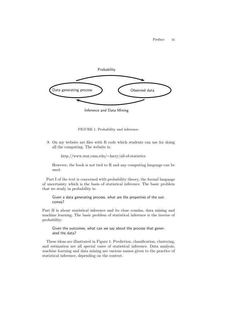
FIGURE 1. Probability and inference.
9. On my website are files with R code which students can use for doingall the computing. The website is:
http://www.stat.cmu.edu/!larry/all-of-statistics
However, the book is not tied to R and any computing language can beused.
Part I of the text is concerned with probability theory, the formal languageof uncertainty which is the basis of statistical inference. The basic problemthat we study in probability is:
Given a data generating process, what are the properties of the out-comes?
Part II is about statistical inference and its close cousins, data mining andmachine learning. The basic problem of statistical inference is the inverse ofprobability:
Given the outcomes, what can we say about the process that gener-ated the data?
These ideas are illustrated in Figure 1. Prediction, classification, clustering,and estimation are all special cases of statistical inference. Data analysis,machine learning and data mining are various names given to the practice ofstatistical inference, depending on the context.
x Preface
Part III applies the ideas from Part II to specific problems such as regres-sion, graphical models, causation, density estimation, smoothing, classifica-tion, and simulation. Part III contains one more chapter on probability thatcovers stochastic processes including Markov chains.
I have drawn on other books in many places. Most chapters contain a sectioncalled Bibliographic Remarks which serves both to acknowledge my debt toother authors and to point readers to other useful references. I would especiallylike to mention the books by DeGroot and Schervish (2002) and Grimmettand Stirzaker (1982) from which I adapted many examples and exercises.
As one develops a book over several years it is easy to lose track of where pre-sentation ideas and, especially, homework problems originated. Some I madeup. Some I remembered from my education. Some I borrowed from otherbooks. I hope I do not o!end anyone if I have used a problem from their bookand failed to give proper credit. As my colleague Mark Schervish wrote in hisbook (Schervish (1995)),
“. . . the problems at the ends of each chapter have come from manysources. . . . These problems, in turn, came from various sourcesunknown to me . . . If I have used a problem without giving propercredit, please take it as a compliment.”
I am indebted to many people without whose help I could not have writtenthis book. First and foremost, the many students who used earlier versionsof this text and provided much feedback. In particular, Liz Prather and Jen-nifer Bakal read the book carefully. Rob Reeder valiantly read through theentire book in excruciating detail and gave me countless suggestions for im-provements. Chris Genovese deserves special mention. He not only providedhelpful ideas about intellectual content, but also spent many, many hourswriting LATEXcode for the book. The best aspects of the book’s layout are dueto his hard work; any stylistic deficiencies are due to my lack of expertise.David Hand, Sam Roweis, and David Scott read the book very carefully andmade numerous suggestions that greatly improved the book. John La!ertyand Peter Spirtes also provided helpful feedback. John Kimmel has been sup-portive and helpful throughout the writing process. Finally, my wife IsabellaVerdinelli has been an invaluable source of love, support, and inspiration.
Larry WassermanPittsburgh, Pennsylvania
July 2003
Preface xi
Statistics/Data Mining Dictionary
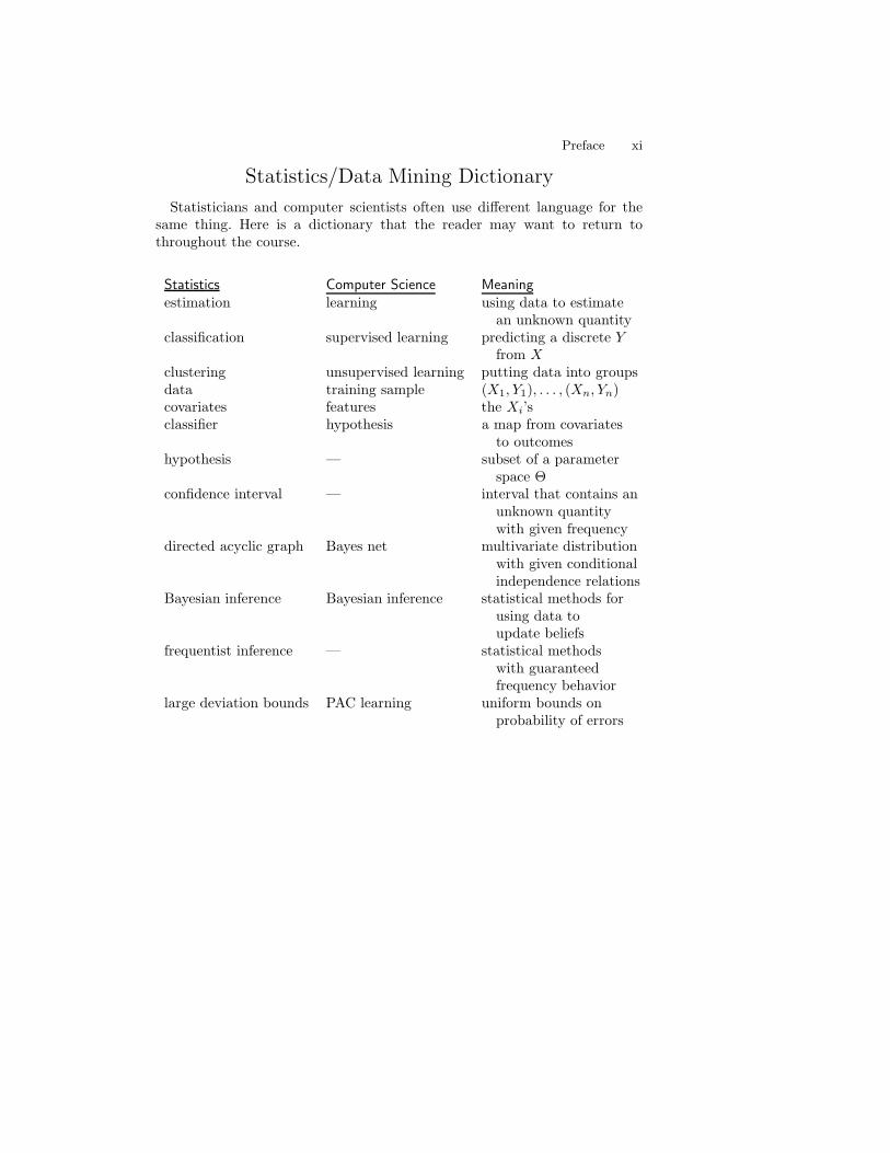
Statisticians and computer scientists often use di!erent language for thesame thing. Here is a dictionary that the reader may want to return tothroughout the course.
Statistics Computer Science Meaningestimation learning using data to estimate
an unknown quantityclassification supervised learning predicting a discrete Y
from Xclustering unsupervised learning putting data into groupsdata training sample (X1, Y1), . . . , (Xn, Yn)covariates features the Xi’sclassifier hypothesis a map from covariates
to outcomeshypothesis — subset of a parameter
space "confidence interval — interval that contains an
unknown quantitywith given frequency
directed acyclic graph Bayes net multivariate distributionwith given conditionalindependence relations
Bayesian inference Bayesian inference statistical methods forusing data toupdate beliefs
frequentist inference — statistical methodswith guaranteedfrequency behavior
large deviation bounds PAC learning uniform bounds onprobability of errors

This is page xiiPrinter: Opaque this
This is page xiiiPrinter: Opaque this
Contents
I Probability
1 Probability 31.1 Introduction . . . . . . . . . . . . . . . . . . . . . . . . . . . . . 31.2 Sample Spaces and Events . . . . . . . . . . . . . . . . . . . . . 31.3 Probability . . . . . . . . . . . . . . . . . . . . . . . . . . . . . 51.4 Probability on Finite Sample Spaces . . . . . . . . . . . . . . . 71.5 Independent Events . . . . . . . . . . . . . . . . . . . . . . . . 81.6 Conditional Probability . . . . . . . . . . . . . . . . . . . . . . 101.7 Bayes’ Theorem . . . . . . . . . . . . . . . . . . . . . . . . . . . 121.8 Bibliographic Remarks . . . . . . . . . . . . . . . . . . . . . . . 131.9 Appendix . . . . . . . . . . . . . . . . . . . . . . . . . . . . . . 131.10 Exercises . . . . . . . . . . . . . . . . . . . . . . . . . . . . . . 13
2 Random Variables 192.1 Introduction . . . . . . . . . . . . . . . . . . . . . . . . . . . . . 192.2 Distribution Functions and Probability Functions . . . . . . . . 202.3 Some Important Discrete Random Variables . . . . . . . . . . . 252.4 Some Important Continuous Random Variables . . . . . . . . . 272.5 Bivariate Distributions . . . . . . . . . . . . . . . . . . . . . . . 312.6 Marginal Distributions . . . . . . . . . . . . . . . . . . . . . . . 332.7 Independent Random Variables . . . . . . . . . . . . . . . . . . 342.8 Conditional Distributions . . . . . . . . . . . . . . . . . . . . . 36
xiv Contents
2.9 Multivariate Distributions and iid Samples . . . . . . . . . . . 382.10 Two Important Multivariate Distributions . . . . . . . . . . . . 392.11 Transformations of Random Variables . . . . . . . . . . . . . . 412.12 Transformations of Several Random Variables . . . . . . . . . . 422.13 Appendix . . . . . . . . . . . . . . . . . . . . . . . . . . . . . . 432.14 Exercises . . . . . . . . . . . . . . . . . . . . . . . . . . . . . . 43
3 Expectation 473.1 Expectation of a Random Variable . . . . . . . . . . . . . . . . 473.2 Properties of Expectations . . . . . . . . . . . . . . . . . . . . . 503.3 Variance and Covariance . . . . . . . . . . . . . . . . . . . . . . 503.4 Expectation and Variance of Important Random Variables . . . 523.5 Conditional Expectation . . . . . . . . . . . . . . . . . . . . . . 543.6 Moment Generating Functions . . . . . . . . . . . . . . . . . . 563.7 Appendix . . . . . . . . . . . . . . . . . . . . . . . . . . . . . . 583.8 Exercises . . . . . . . . . . . . . . . . . . . . . . . . . . . . . . 58
4 Inequalities 634.1 Probability Inequalities . . . . . . . . . . . . . . . . . . . . . . 634.2 Inequalities For Expectations . . . . . . . . . . . . . . . . . . . 664.3 Bibliographic Remarks . . . . . . . . . . . . . . . . . . . . . . . 664.4 Appendix . . . . . . . . . . . . . . . . . . . . . . . . . . . . . . 674.5 Exercises . . . . . . . . . . . . . . . . . . . . . . . . . . . . . . 68
5 Convergence of Random Variables 715.1 Introduction . . . . . . . . . . . . . . . . . . . . . . . . . . . . . 715.2 Types of Convergence . . . . . . . . . . . . . . . . . . . . . . . 725.3 The Law of Large Numbers . . . . . . . . . . . . . . . . . . . . 765.4 The Central Limit Theorem . . . . . . . . . . . . . . . . . . . . 775.5 The Delta Method . . . . . . . . . . . . . . . . . . . . . . . . . 795.6 Bibliographic Remarks . . . . . . . . . . . . . . . . . . . . . . . 805.7 Appendix . . . . . . . . . . . . . . . . . . . . . . . . . . . . . . 81
5.7.1 Almost Sure and L1 Convergence . . . . . . . . . . . . . 815.7.2 Proof of the Central Limit Theorem . . . . . . . . . . . 81
5.8 Exercises . . . . . . . . . . . . . . . . . . . . . . . . . . . . . . 82
II Statistical Inference
6 Models, Statistical Inference and Learning 876.1 Introduction . . . . . . . . . . . . . . . . . . . . . . . . . . . . . 876.2 Parametric and Nonparametric Models . . . . . . . . . . . . . . 876.3 Fundamental Concepts in Inference . . . . . . . . . . . . . . . . 90
6.3.1 Point Estimation . . . . . . . . . . . . . . . . . . . . . . 906.3.2 Confidence Sets . . . . . . . . . . . . . . . . . . . . . . . 92
Contents xv
6.3.3 Hypothesis Testing . . . . . . . . . . . . . . . . . . . . . 946.4 Bibliographic Remarks . . . . . . . . . . . . . . . . . . . . . . . 956.5 Appendix . . . . . . . . . . . . . . . . . . . . . . . . . . . . . . 956.6 Exercises . . . . . . . . . . . . . . . . . . . . . . . . . . . . . . 95
7 Estimating the cdf and Statistical Functionals 977.1 The Empirical Distribution Function . . . . . . . . . . . . . . . 977.2 Statistical Functionals . . . . . . . . . . . . . . . . . . . . . . . 997.3 Bibliographic Remarks . . . . . . . . . . . . . . . . . . . . . . . 1047.4 Exercises . . . . . . . . . . . . . . . . . . . . . . . . . . . . . . 104
8 The Bootstrap 1078.1 Simulation . . . . . . . . . . . . . . . . . . . . . . . . . . . . . . 1088.2 Bootstrap Variance Estimation . . . . . . . . . . . . . . . . . . 1088.3 Bootstrap Confidence Intervals . . . . . . . . . . . . . . . . . . 1108.4 Bibliographic Remarks . . . . . . . . . . . . . . . . . . . . . . . 1158.5 Appendix . . . . . . . . . . . . . . . . . . . . . . . . . . . . . . 115
8.5.1 The Jackknife . . . . . . . . . . . . . . . . . . . . . . . . 1158.5.2 Justification For The Percentile Interval . . . . . . . . . 116
8.6 Exercises . . . . . . . . . . . . . . . . . . . . . . . . . . . . . . 116
9 Parametric Inference 1199.1 Parameter of Interest . . . . . . . . . . . . . . . . . . . . . . . . 1209.2 The Method of Moments . . . . . . . . . . . . . . . . . . . . . . 1209.3 Maximum Likelihood . . . . . . . . . . . . . . . . . . . . . . . . 1229.4 Properties of Maximum Likelihood Estimators . . . . . . . . . 1249.5 Consistency of Maximum Likelihood Estimators . . . . . . . . . 1269.6 Equivariance of the mle . . . . . . . . . . . . . . . . . . . . . . 1279.7 Asymptotic Normality . . . . . . . . . . . . . . . . . . . . . . . 1289.8 Optimality . . . . . . . . . . . . . . . . . . . . . . . . . . . . . 1309.9 The Delta Method . . . . . . . . . . . . . . . . . . . . . . . . . 1319.10 Multiparameter Models . . . . . . . . . . . . . . . . . . . . . . 1339.11 The Parametric Bootstrap . . . . . . . . . . . . . . . . . . . . . 1349.12 Checking Assumptions . . . . . . . . . . . . . . . . . . . . . . . 1359.13 Appendix . . . . . . . . . . . . . . . . . . . . . . . . . . . . . . 135
9.13.1 Proofs . . . . . . . . . . . . . . . . . . . . . . . . . . . . 1359.13.2 Su#ciency . . . . . . . . . . . . . . . . . . . . . . . . . . 1379.13.3 Exponential Families . . . . . . . . . . . . . . . . . . . . 1409.13.4 Computing Maximum Likelihood Estimates . . . . . . . 142
9.14 Exercises . . . . . . . . . . . . . . . . . . . . . . . . . . . . . . 146
10 Hypothesis Testing and p-values 14910.1 The Wald Test . . . . . . . . . . . . . . . . . . . . . . . . . . . 15210.2 p-values . . . . . . . . . . . . . . . . . . . . . . . . . . . . . . . 15610.3 The !2 Distribution . . . . . . . . . . . . . . . . . . . . . . . . 159
xvi Contents
10.4 Pearson’s !2 Test For Multinomial Data . . . . . . . . . . . . . 16010.5 The Permutation Test . . . . . . . . . . . . . . . . . . . . . . . 16110.6 The Likelihood Ratio Test . . . . . . . . . . . . . . . . . . . . . 16410.7 Multiple Testing . . . . . . . . . . . . . . . . . . . . . . . . . . 16510.8 Goodness-of-fit Tests . . . . . . . . . . . . . . . . . . . . . . . . 16810.9 Bibliographic Remarks . . . . . . . . . . . . . . . . . . . . . . . 16910.10Appendix . . . . . . . . . . . . . . . . . . . . . . . . . . . . . . 170
10.10.1The Neyman-Pearson Lemma . . . . . . . . . . . . . . . 17010.10.2The t-test . . . . . . . . . . . . . . . . . . . . . . . . . . 170
10.11Exercises . . . . . . . . . . . . . . . . . . . . . . . . . . . . . . 170
11 Bayesian Inference 17511.1 The Bayesian Philosophy . . . . . . . . . . . . . . . . . . . . . 17511.2 The Bayesian Method . . . . . . . . . . . . . . . . . . . . . . . 17611.3 Functions of Parameters . . . . . . . . . . . . . . . . . . . . . . 18011.4 Simulation . . . . . . . . . . . . . . . . . . . . . . . . . . . . . . 18011.5 Large Sample Properties of Bayes’ Procedures . . . . . . . . . . 18111.6 Flat Priors, Improper Priors, and “Noninformative” Priors . . . 18111.7 Multiparameter Problems . . . . . . . . . . . . . . . . . . . . . 18311.8 Bayesian Testing . . . . . . . . . . . . . . . . . . . . . . . . . . 18411.9 Strengths and Weaknesses of Bayesian Inference . . . . . . . . 18511.10Bibliographic Remarks . . . . . . . . . . . . . . . . . . . . . . . 18911.11Appendix . . . . . . . . . . . . . . . . . . . . . . . . . . . . . . 19011.12Exercises . . . . . . . . . . . . . . . . . . . . . . . . . . . . . . 190
12 Statistical Decision Theory 19312.1 Preliminaries . . . . . . . . . . . . . . . . . . . . . . . . . . . . 19312.2 Comparing Risk Functions . . . . . . . . . . . . . . . . . . . . . 19412.3 Bayes Estimators . . . . . . . . . . . . . . . . . . . . . . . . . . 19712.4 Minimax Rules . . . . . . . . . . . . . . . . . . . . . . . . . . . 19812.5 Maximum Likelihood, Minimax, and Bayes . . . . . . . . . . . 20112.6 Admissibility . . . . . . . . . . . . . . . . . . . . . . . . . . . . 20212.7 Stein’s Paradox . . . . . . . . . . . . . . . . . . . . . . . . . . . 20412.8 Bibliographic Remarks . . . . . . . . . . . . . . . . . . . . . . . 20412.9 Exercises . . . . . . . . . . . . . . . . . . . . . . . . . . . . . . 204
III Statistical Models and Methods
13 Linear and Logistic Regression 20913.1 Simple Linear Regression . . . . . . . . . . . . . . . . . . . . . 20913.2 Least Squares and Maximum Likelihood . . . . . . . . . . . . . 21213.3 Properties of the Least Squares Estimators . . . . . . . . . . . 21413.4 Prediction . . . . . . . . . . . . . . . . . . . . . . . . . . . . . . 21513.5 Multiple Regression . . . . . . . . . . . . . . . . . . . . . . . . 216
Contents xvii
13.6 Model Selection . . . . . . . . . . . . . . . . . . . . . . . . . . . 21813.7 Logistic Regression . . . . . . . . . . . . . . . . . . . . . . . . . 22313.8 Bibliographic Remarks . . . . . . . . . . . . . . . . . . . . . . . 22513.9 Appendix . . . . . . . . . . . . . . . . . . . . . . . . . . . . . . 22513.10Exercises . . . . . . . . . . . . . . . . . . . . . . . . . . . . . . 226
14 Multivariate Models 23114.1 Random Vectors . . . . . . . . . . . . . . . . . . . . . . . . . . 23214.2 Estimating the Correlation . . . . . . . . . . . . . . . . . . . . 23314.3 Multivariate Normal . . . . . . . . . . . . . . . . . . . . . . . . 23414.4 Multinomial . . . . . . . . . . . . . . . . . . . . . . . . . . . . . 23514.5 Bibliographic Remarks . . . . . . . . . . . . . . . . . . . . . . . 23714.6 Appendix . . . . . . . . . . . . . . . . . . . . . . . . . . . . . . 23714.7 Exercises . . . . . . . . . . . . . . . . . . . . . . . . . . . . . . 238
15 Inference About Independence 23915.1 Two Binary Variables . . . . . . . . . . . . . . . . . . . . . . . 23915.2 Two Discrete Variables . . . . . . . . . . . . . . . . . . . . . . . 24315.3 Two Continuous Variables . . . . . . . . . . . . . . . . . . . . . 24415.4 One Continuous Variable and One Discrete . . . . . . . . . . . 24415.5 Appendix . . . . . . . . . . . . . . . . . . . . . . . . . . . . . . 24515.6 Exercises . . . . . . . . . . . . . . . . . . . . . . . . . . . . . . 248
16 Causal Inference 25116.1 The Counterfactual Model . . . . . . . . . . . . . . . . . . . . . 25116.2 Beyond Binary Treatments . . . . . . . . . . . . . . . . . . . . 25516.3 Observational Studies and Confounding . . . . . . . . . . . . . 25716.4 Simpson’s Paradox . . . . . . . . . . . . . . . . . . . . . . . . . 25916.5 Bibliographic Remarks . . . . . . . . . . . . . . . . . . . . . . . 26116.6 Exercises . . . . . . . . . . . . . . . . . . . . . . . . . . . . . . 261
17 Directed Graphs and Conditional Independence 26317.1 Introduction . . . . . . . . . . . . . . . . . . . . . . . . . . . . . 26317.2 Conditional Independence . . . . . . . . . . . . . . . . . . . . . 26417.3 DAGs . . . . . . . . . . . . . . . . . . . . . . . . . . . . . . . . 26417.4 Probability and DAGs . . . . . . . . . . . . . . . . . . . . . . . 26617.5 More Independence Relations . . . . . . . . . . . . . . . . . . . 26717.6 Estimation for DAGs . . . . . . . . . . . . . . . . . . . . . . . . 27217.7 Bibliographic Remarks . . . . . . . . . . . . . . . . . . . . . . . 27217.8 Appendix . . . . . . . . . . . . . . . . . . . . . . . . . . . . . . 27217.9 Exercises . . . . . . . . . . . . . . . . . . . . . . . . . . . . . . 276
18 Undirected Graphs 28118.1 Undirected Graphs . . . . . . . . . . . . . . . . . . . . . . . . . 28118.2 Probability and Graphs . . . . . . . . . . . . . . . . . . . . . . 282
xviii Contents
18.3 Cliques and Potentials . . . . . . . . . . . . . . . . . . . . . . . 28518.4 Fitting Graphs to Data . . . . . . . . . . . . . . . . . . . . . . 28618.5 Bibliographic Remarks . . . . . . . . . . . . . . . . . . . . . . . 28618.6 Exercises . . . . . . . . . . . . . . . . . . . . . . . . . . . . . . 286
19 Log-Linear Models 29119.1 The Log-Linear Model . . . . . . . . . . . . . . . . . . . . . . . 29119.2 Graphical Log-Linear Models . . . . . . . . . . . . . . . . . . . 29419.3 Hierarchical Log-Linear Models . . . . . . . . . . . . . . . . . . 29619.4 Model Generators . . . . . . . . . . . . . . . . . . . . . . . . . . 29719.5 Fitting Log-Linear Models to Data . . . . . . . . . . . . . . . . 29819.6 Bibliographic Remarks . . . . . . . . . . . . . . . . . . . . . . . 30019.7 Exercises . . . . . . . . . . . . . . . . . . . . . . . . . . . . . . 301
20 Nonparametric Curve Estimation 30320.1 The Bias-Variance Tradeo! . . . . . . . . . . . . . . . . . . . . 30420.2 Histograms . . . . . . . . . . . . . . . . . . . . . . . . . . . . . 30520.3 Kernel Density Estimation . . . . . . . . . . . . . . . . . . . . . 31220.4 Nonparametric Regression . . . . . . . . . . . . . . . . . . . . . 31920.5 Appendix . . . . . . . . . . . . . . . . . . . . . . . . . . . . . . 32420.6 Bibliographic Remarks . . . . . . . . . . . . . . . . . . . . . . . 32520.7 Exercises . . . . . . . . . . . . . . . . . . . . . . . . . . . . . . 325
21 Smoothing Using Orthogonal Functions 32721.1 Orthogonal Functions and L2 Spaces . . . . . . . . . . . . . . . 32721.2 Density Estimation . . . . . . . . . . . . . . . . . . . . . . . . . 33121.3 Regression . . . . . . . . . . . . . . . . . . . . . . . . . . . . . . 33521.4 Wavelets . . . . . . . . . . . . . . . . . . . . . . . . . . . . . . . 34021.5 Appendix . . . . . . . . . . . . . . . . . . . . . . . . . . . . . . 34521.6 Bibliographic Remarks . . . . . . . . . . . . . . . . . . . . . . . 34621.7 Exercises . . . . . . . . . . . . . . . . . . . . . . . . . . . . . . 346
22 Classification 34922.1 Introduction . . . . . . . . . . . . . . . . . . . . . . . . . . . . . 34922.2 Error Rates and the Bayes Classifier . . . . . . . . . . . . . . . 35022.3 Gaussian and Linear Classifiers . . . . . . . . . . . . . . . . . . 35322.4 Linear Regression and Logistic Regression . . . . . . . . . . . . 35622.5 Relationship Between Logistic Regression and LDA . . . . . . . 35822.6 Density Estimation and Naive Bayes . . . . . . . . . . . . . . . 35922.7 Trees . . . . . . . . . . . . . . . . . . . . . . . . . . . . . . . . . 36022.8 Assessing Error Rates and Choosing a Good Classifier . . . . . 36222.9 Support Vector Machines . . . . . . . . . . . . . . . . . . . . . 36822.10Kernelization . . . . . . . . . . . . . . . . . . . . . . . . . . . . 37122.11Other Classifiers . . . . . . . . . . . . . . . . . . . . . . . . . . 37522.12Bibliographic Remarks . . . . . . . . . . . . . . . . . . . . . . . 377
Contents xix
22.13Exercises . . . . . . . . . . . . . . . . . . . . . . . . . . . . . . 377
23 Probability Redux: Stochastic Processes 38123.1 Introduction . . . . . . . . . . . . . . . . . . . . . . . . . . . . . 38123.2 Markov Chains . . . . . . . . . . . . . . . . . . . . . . . . . . . 38323.3 Poisson Processes . . . . . . . . . . . . . . . . . . . . . . . . . . 39423.4 Bibliographic Remarks . . . . . . . . . . . . . . . . . . . . . . . 39723.5 Exercises . . . . . . . . . . . . . . . . . . . . . . . . . . . . . . 398
24 Simulation Methods 40324.1 Bayesian Inference Revisited . . . . . . . . . . . . . . . . . . . . 40324.2 Basic Monte Carlo Integration . . . . . . . . . . . . . . . . . . 40424.3 Importance Sampling . . . . . . . . . . . . . . . . . . . . . . . . 40824.4 MCMC Part I: The Metropolis–Hastings Algorithm . . . . . . 41124.5 MCMC Part II: Di!erent Flavors . . . . . . . . . . . . . . . . . 41524.6 Bibliographic Remarks . . . . . . . . . . . . . . . . . . . . . . . 42024.7 Exercises . . . . . . . . . . . . . . . . . . . . . . . . . . . . . . 420
Index

This is page xxPrinter: Opaque this

Part I
Probability

This is pagePrinter: Opaque this
This is page 3Printer: Opaque this
1Probability
1.1 Introduction
Probability is a mathematical language for quantifying uncertainty. In thisChapter we introduce the basic concepts underlying probability theory. Webegin with the sample space, which is the set of possible outcomes.
1.2 Sample Spaces and Events
The sample space $ is the set of possible outcomes of an experiment. Points" in $ are called sample outcomes, realizations, or elements. Subsets of$ are called Events.
1.1 Example. If we toss a coin twice then $ = {HH, HT, TH, TT }. The eventthat the first toss is heads is A = {HH, HT }. !
1.2 Example. Let " be the outcome of a measurement of some physical quan-tity, for example, temperature. Then $ = R = ("#,#). One could argue thattaking $ = R is not accurate since temperature has a lower bound. But thereis usually no harm in taking the sample space to be larger than needed. Theevent that the measurement is larger than 10 but less than or equal to 23 isA = (10, 23]. !
4 1. Probability
1.3 Example. If we toss a coin forever, then the sample space is the infiniteset
$ =!" = ("1,"2,"3, . . . , ) : "i $ {H, T }
".
Let E be the event that the first head appears on the third toss. Then
E =!
("1,"2,"3, . . . , ) : "1 = T,"2 = T,"3 = H, "i $ {H, T } for i > 3". !
Given an event A, let Ac = {" $ $ : " /$ A} denote the complement ofA. Informally, Ac can be read as “not A.” The complement of $ is the emptyset %. The union of events A and B is defined
A#
B = {" $ $ : " $ A or " $ B or " $ both}
which can be thought of as “A or B.” If A1, A2, . . . is a sequence of sets then!#
i=1
Ai =!" $ $ : " $ Ai for at least one i
".
The intersection of A and B is
A$
B = {" $ $ : " $ A and " $ B}
read “A and B.” Sometimes we write A%
B as AB or (A, B). If A1, A2, . . . isa sequence of sets then
!$
i=1
Ai =!" $ $ : " $ Ai for all i
".
The set di!erence is defined by A"B = {" : " $ A," /$ B}. If every elementof A is also contained in B we write A & B or, equivalently, B ' A. If A is afinite set, let |A| denote the number of elements in A. See the following tablefor a summary.
Summary of Terminology$ sample space" outcome (point or element)A event (subset of $)Ac complement of A (not A)A&
B union (A or B)A%
B or AB intersection (A and B)A"B set di!erence (" in A but not in B)A & B set inclusion% null event (always false)$ true event (always true)
1.3 Probability 5
We say that A1, A2, . . . are disjoint or are mutually exclusive if Ai%
Aj =% whenever i (= j. For example, A1 = [0, 1), A2 = [1, 2), A3 = [2, 3), . . . aredisjoint. A partition of $ is a sequence of disjoint sets A1, A2, . . . such that&!
i=1 Ai = $. Given an event A, define the indicator function of A by
IA(") = I(" $ A) ='
1 if " $ A0 if " /$ A.
A sequence of sets A1, A2, . . . is monotone increasing if A1 & A2 &· · · and we define limn"! An =
&!i=1 Ai. A sequence of sets A1, A2, . . . is
monotone decreasing if A1 ' A2 ' · · · and then we define limn"! An =%!i=1 Ai. In either case, we will write An ) A.
1.4 Example. Let $ = R and let Ai = [0, 1/i) for i = 1, 2, . . .. Then&!
i=1 Ai =[0, 1) and
%!i=1 Ai = {0}. If instead we define Ai = (0, 1/i) then
&!i=1 Ai =
(0, 1) and%!
i=1 Ai = %. !
1.3 Probability
We will assign a real number P(A) to every event A, called the probability ofA. 1 We also call P a probability distribution or a probability measure.To qualify as a probability, P must satisfy three axioms:
1.5 Definition. A function P that assigns a real number P(A) to eachevent A is a probability distribution or a probability measure if itsatisfies the following three axioms:Axiom 1: P(A) * 0 for every A
Axiom 2: P($) = 1Axiom 3: If A1, A2, . . . are disjoint then
P( !#
i=1
Ai
)=
!*
i=1
P(Ai).
1It is not always possible to assign a probability to every event A if the sample space is large,such as the whole real line. Instead, we assign probabilities to a limited class of set called aσ-field. See the appendix for details.
6 1. Probability
There are many interpretations of P(A). The two common interpretationsare frequencies and degrees of beliefs. In the frequency interpretation, P(A)is the long run proportion of times that A is true in repetitions. For example,if we say that the probability of heads is 1/2, we mean that if we flip thecoin many times then the proportion of times we get heads tends to 1/2 asthe number of tosses increases. An infinitely long, unpredictable sequence oftosses whose limiting proportion tends to a constant is an idealization, muchlike the idea of a straight line in geometry. The degree-of-belief interpretationis that P(A) measures an observer’s strength of belief that A is true. In eitherinterpretation, we require that Axioms 1 to 3 hold. The di!erence in inter-pretation will not matter much until we deal with statistical inference. There,the di!ering interpretations lead to two schools of inference: the frequentistand the Bayesian schools. We defer discussion until Chapter 11.
One can derive many properties of P from the axioms, such as:
P(%) = 0
A & B =+ P(A) , P(B)
0 , P(A) , 1
P(Ac) = 1" P(A)
A$
B = % =+ P+A#
B,
= P(A) + P(B). (1.1)
A less obvious property is given in the following Lemma.
1.6 Lemma. For any events A and B,
P+A#
B,
= P(A) + P(B)" P(AB).
Proof. Write A&
B = (ABc)&
(AB)&
(AcB) and note that these eventsare disjoint. Hence, making repeated use of the fact that P is additive fordisjoint events, we see that
P+A#
B,
= P+(ABc)
#(AB)
#(AcB)
,
= P(ABc) + P(AB) + P(AcB)
= P(ABc) + P(AB) + P(AcB) + P(AB)" P(AB)
= P+(ABc)
#(AB)
,+ P
+(AcB)
#(AB)
," P(AB)
= P(A) + P(B)" P(AB). !
1.7 Example. Two coin tosses. Let H1 be the event that heads occurs ontoss 1 and let H2 be the event that heads occurs on toss 2. If all outcomes are
1.4 Probability on Finite Sample Spaces 7
equally likely, then P(H1&
H2) = P(H1)+P(H2)"P(H1H2) = 12+ 1
2"14 = 3/4.
!
1.8 Theorem (Continuity of Probabilities). If An ) A then
P(An)) P(A)
as n)#.
Proof. Suppose that An is monotone increasing so that A1 & A2 & · · ·.Let A = limn"! An =
&!i=1 Ai. Define B1 = A1, B2 = {" $ $ : " $
A2," /$ A1}, B3 = {" $ $ : " $ A3," /$ A2," /$ A1}, . . . It can beshown that B1, B2, . . . are disjoint, An =
&ni=1 Ai =
&ni=1 Bi for each n and&!
i=1 Bi =&!
i=1 Ai. (See exercise 1.) From Axiom 3,
P(An) = P(
n#
i=1
Bi
)=
n*
i=1
P(Bi)
and hence, using Axiom 3 again,
limn"!
P(An) = limn"!
n*
i=1
P(Bi) =!*
i=1
P(Bi) = P( !#
i=1
Bi
)= P(A). !
1.4 Probability on Finite Sample Spaces
Suppose that the sample space $ = {"1, . . . ,"n} is finite. For example, if wetoss a die twice, then $ has 36 elements: $ = {(i, j); i, j $ {1, . . . 6}}. If eachoutcome is equally likely, then P(A) = |A|/36 where |A| denotes the numberof elements in A. The probability that the sum of the dice is 11 is 2/36 sincethere are two outcomes that correspond to this event.
If $ is finite and if each outcome is equally likely, then
P(A) =|A||$| ,
which is called the uniform probability distribution. To compute prob-abilities, we need to count the number of points in an event A. Methods forcounting points are called combinatorial methods. We needn’t delve into thesein any great detail. We will, however, need a few facts from counting theorythat will be useful later. Given n objects, the number of ways of ordering
8 1. Probability
these objects is n! = n(n " 1)(n " 2) · · · 3 · 2 · 1. For convenience, we define0! = 1. We also define -
n
k
.=
n!k!(n" k)!
, (1.2)
read “n choose k”, which is the number of distinct ways of choosing k objectsfrom n. For example, if we have a class of 20 people and we want to select acommittee of 3 students, then there are
-203
.=
20!3!17!
=20- 19- 18
3- 2- 1= 1140
possible committees. We note the following properties:-
n
0
.=-
n
n
.= 1 and
-n
k
.=-
n
n" k
..
1.5 Independent Events
If we flip a fair coin twice, then the probability of two heads is 12 -
12 . We
multiply the probabilities because we regard the two tosses as independent.The formal definition of independence is as follows:
1.9 Definition. Two events A and B are independent if
P(AB) = P(A)P(B) (1.3)
and we write A ! B. A set of events {Ai : i $ I} is independent if
P($
i#J
Ai
)=/
i#J
P(Ai)
for every finite subset J of I. If A and B are not independent, we write
A !""""# B
Independence can arise in two distinct ways. Sometimes, we explicitly as-sume that two events are independent. For example, in tossing a coin twice,we usually assume the tosses are independent which reflects the fact that thecoin has no memory of the first toss. In other instances, we derive indepen-dence by verifying that P(AB) = P(A)P(B) holds. For example, in tossinga fair die, let A = {2, 4, 6} and let B = {1, 2, 3, 4}. Then, A
%B = {2, 4},
1.5 Independent Events 9
P(AB) = 2/6 = P(A)P(B) = (1/2)- (2/3) and so A and B are independent.In this case, we didn’t assume that A and B are independent — it just turnedout that they were.
Suppose that A and B are disjoint events, each with positive probability.Can they be independent? No. This follows since P(A)P(B) > 0 yet P(AB) =P(%) = 0. Except in this special case, there is no way to judge independenceby looking at the sets in a Venn diagram.
1.10 Example. Toss a fair coin 10 times. Let A =“at least one head.” Let Tj
be the event that tails occurs on the jth toss. Then
P(A) = 1" P(Ac)
= 1" P(all tails)
= 1" P(T1T2 · · ·T10)
= 1" P(T1)P(T2) · · ·P(T10) using independence
= 1"-
12
.10
. .999. !
1.11 Example. Two people take turns trying to sink a basketball into a net.Person 1 succeeds with probability 1/3 while person 2 succeeds with proba-bility 1/4. What is the probability that person 1 succeeds before person 2?Let E denote the event of interest. Let Aj be the event that the first successis by person 1 and that it occurs on trial number j. Note that A1, A2, . . . aredisjoint and that E =
&!j=1 Aj . Hence,
P(E) =!*
j=1
P(Aj).
Now, P(A1) = 1/3. A2 occurs if we have the sequence person 1 misses, person2 misses, person 1 succeeds. This has probability P(A2) = (2/3)(3/4)(1/3) =(1/2)(1/3). Following this logic we see that P(Aj) = (1/2)j$1(1/3). Hence,
P(E) =!*
j=1
13
-12
.j$1
=13
!*
j=1
-12
.j$1
=23.
Here we used that fact that, if 0 < r < 1 then0!
j=k rj = rk/(1" r). !
10 1. Probability
Summary of Independence
1. A and B are independent if and only if P(AB) = P(A)P(B).
2. Independence is sometimes assumed and sometimes derived.
3. Disjoint events with positive probability are not independent.
1.6 Conditional Probability
Assuming that P(B) > 0, we define the conditional probability of A giventhat B has occurred as follows:
1.12 Definition. If P(B) > 0 then the conditional probability of A
given B is
P(A|B) =P(AB)P(B)
. (1.4)
Think of P(A|B) as the fraction of times A occurs among those in whichB occurs. For any fixed B such that P(B) > 0, P(·|B) is a probability (i.e., itsatisfies the three axioms of probability). In particular, P(A|B) * 0, P($|B) =1 and if A1, A2, . . . are disjoint then P(
&!i=1 Ai|B) =
0!i=1 P(Ai|B). But it
is in general not true that P(A|B&
C) = P(A|B) + P(A|C). The rules ofprobability apply to events on the left of the bar. In general it is not the casethat P(A|B) = P(B|A). People get this confused all the time. For example,the probability of spots given you have measles is 1 but the probability thatyou have measles given that you have spots is not 1. In this case, the di!erencebetween P(A|B) and P(B|A) is obvious but there are cases where it is lessobvious. This mistake is made often enough in legal cases that it is sometimescalled the prosecutor’s fallacy.
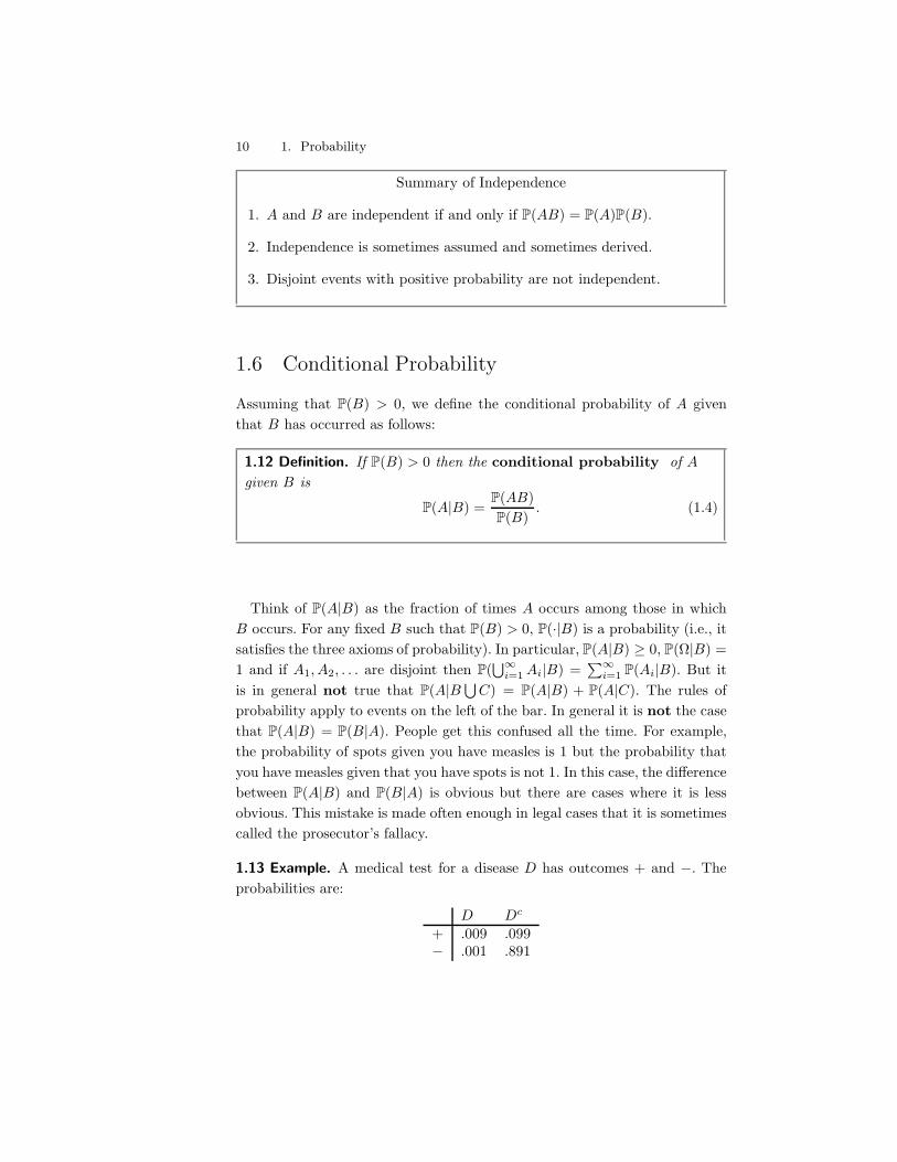
1.13 Example. A medical test for a disease D has outcomes + and ". Theprobabilities are:
D Dc
+ .009 .099" .001 .891
1.6 Conditional Probability 11
From the definition of conditional probability,
P(+|D) =P(+
%D)
P(D)=
.009.009 + .001
= .9
andP("|Dc) =
P("%
Dc)P(Dc)
=.891
.891 + .099. .9.
Apparently, the test is fairly accurate. Sick people yield a positive 90 percentof the time and healthy people yield a negative about 90 percent of the time.Suppose you go for a test and get a positive. What is the probability you havethe disease? Most people answer .90. The correct answer is
P(D|+) =P(+
%D)
P(+)=
.009.009 + .099
. .08.
The lesson here is that you need to compute the answer numerically. Don’ttrust your intuition. !
The results in the next lemma follow directly from the definition of condi-tional probability.
1.14 Lemma. If A and B are independent events then P(A|B) = P(A). Also,for any pair of events A and B,
P(AB) = P(A|B)P(B) = P(B|A)P(A).
From the last lemma, we see that another interpretation of independence isthat knowing B doesn’t change the probability of A. The formula P(AB) =P(A)P(B|A) is sometimes helpful for calculating probabilities.
1.15 Example. Draw two cards from a deck, without replacement. Let A bethe event that the first draw is the Ace of Clubs and let B be the event thatthe second draw is the Queen of Diamonds. Then P(AB) = P(A)P(B|A) =(1/52)- (1/51). !
Summary of Conditional Probability
1. If P(B) > 0, then
P(A|B) =P(AB)P(B)
.
2. P(·|B) satisfies the axioms of probability, for fixed B. In general,P(A|·) does not satisfy the axioms of probability, for fixed A.
3. In general, P(A|B) (= P(B|A).
12 1. Probability
4. A and B are independent if and only if P(A|B) = P(A).
1.7 Bayes’ Theorem
Bayes’ theorem is the basis of “expert systems” and “Bayes’ nets,” which arediscussed in Chapter 17. First, we need a preliminary result.
1.16 Theorem (The Law of Total Probability). Let A1, . . . , Ak be a partitionof $. Then, for any event B,
P(B) =k*
i=1
P(B|Ai)P(Ai).
Proof. Define Cj = BAj and note that C1, . . . , Ck are disjoint and thatB =
&kj=1 Cj . Hence,
P(B) =*
j
P(Cj) =*
j
P(BAj) =*
j
P(B|Aj)P(Aj)
since P(BAj) = P(B|Aj)P(Aj) from the definition of conditional probability.!
1.17 Theorem (Bayes’ Theorem). Let A1, . . . , Ak be a partition of $ suchthat P(Ai) > 0 for each i. If P(B) > 0 then, for each i = 1, . . . , k,
P(Ai|B) =P(B|Ai)P(Ai)0j P(B|Aj)P(Aj)
. (1.5)
1.18 Remark. We call P(Ai) the prior probability of A and P(Ai|B) theposterior probability of A.
Proof. We apply the definition of conditional probability twice, followedby the law of total probability:
P(Ai|B) =P(AiB)P(B)
=P(B|Ai)P(Ai)
P(B)=
P(B|Ai)P(Ai)0j P(B|Aj)P(Aj)
. !
1.19 Example. I divide my email into three categories: A1 = “spam,” A2 =“low priority” and A3 = “high priority.” From previous experience I find that
1.8 Bibliographic Remarks 13
P(A1) = .7, P(A2) = .2 and P(A3) = .1. Of course, .7 + .2 + .1 = 1. Let B bethe event that the email contains the word “free.” From previous experience,P(B|A1) = .9, P(B|A2) = .01, P(B|A1) = .01. (Note: .9 + .01 + .01 (= 1.) Ireceive an email with the word “free.” What is the probability that it is spam?Bayes’ theorem yields,
P(A1|B) =.9- .7
(.9- .7) + (.01- .2) + (.01- .1)= .995. !
1.8 Bibliographic Remarks
The material in this chapter is standard. Details can be found in any numberof books. At the introductory level, there is DeGroot and Schervish (2002);at the intermediate level, Grimmett and Stirzaker (1982) and Karr (1993); atthe advanced level there are Billingsley (1979) and Breiman (1992). I adaptedmany examples and exercises from DeGroot and Schervish (2002) and Grim-mett and Stirzaker (1982).
1.9 Appendix
Generally, it is not feasible to assign probabilities to all subsets of a samplespace $. Instead, one restricts attention to a set of events called a #-algebraor a #-field which is a class A that satisfies:
(i) % $ A,(ii) if A1, A2, . . . ,$ A then
&!i=1 Ai $ A and
(iii) A $ A implies that Ac $ A.The sets in A are said to be measurable. We call ($,A) a measurablespace. If P is a probability measure defined on A, then ($,A, P) is called aprobability space. When $ is the real line, we take A to be the smallest#-field that contains all the open subsets, which is called the Borel #-field.
1.10 Exercises
1. Fill in the details of the proof of Theorem 1.8. Also, prove the monotonedecreasing case.
2. Prove the statements in equation (1.1).
14 1. Probability
3. Let $ be a sample space and let A1, A2, . . . , be events. Define Bn =&!i=n Ai and Cn =
%!i=n Ai.
(a) Show that B1 ' B2 ' · · · and that C1 & C2 & · · ·.
(b) Show that " $%!
n=1 Bn if and only if " belongs to an infinitenumber of the events A1, A2, . . ..
(c) Show that " $&!
n=1 Cn if and only if " belongs to all the eventsA1, A2, . . . except possibly a finite number of those events.
4. Let {Ai : i $ I} be a collection of events where I is an arbitrary indexset. Show that
(#
i#I
Ai
)c
=$
i#I
Aci and
($
i#I
Ai
)c
=#
i#I
Aci
Hint: First prove this for I = {1, . . . , n}.
5. Suppose we toss a fair coin until we get exactly two heads. Describethe sample space S. What is the probability that exactly k tosses arerequired?
6. Let $ = {0, 1, . . . , }. Prove that there does not exist a uniform distri-bution on $ (i.e., if P(A) = P(B) whenever |A| = |B|, then P cannotsatisfy the axioms of probability).
7. Let A1, A2, . . . be events. Show that
P( !#
n=1
An
),
!*
n=1
P (An) .
Hint: Define Bn = An "&n$1
i=1 Ai. Then show that the Bn are disjointand that
&!n=1 An =
&!n=1 Bn.
8. Suppose that P(Ai) = 1 for each i. Prove that
P( !$
i=1
Ai
)= 1.
9. For fixed B such that P(B) > 0, show that P(·|B) satisfies the axiomsof probability.
10. You have probably heard it before. Now you can solve it rigorously.It is called the “Monty Hall Problem.” A prize is placed at random
1.10 Exercises 15
behind one of three doors. You pick a door. To be concrete, let’s supposeyou always pick door 1. Now Monty Hall chooses one of the other twodoors, opens it and shows you that it is empty. He then gives you theopportunity to keep your door or switch to the other unopened door.Should you stay or switch? Intuition suggests it doesn’t matter. Thecorrect answer is that you should switch. Prove it. It will help to specifythe sample space and the relevant events carefully. Thus write $ ={("1,"2) : "i $ {1, 2, 3}} where "1 is where the prize is and "2 is thedoor Monty opens.
11. Suppose that A and B are independent events. Show that Ac and Bc
are independent events.
12. There are three cards. The first is green on both sides, the second is redon both sides and the third is green on one side and red on the other. Wechoose a card at random and we see one side (also chosen at random).If the side we see is green, what is the probability that the other side isalso green? Many people intuitively answer 1/2. Show that the correctanswer is 2/3.
13. Suppose that a fair coin is tossed repeatedly until both a head and tailhave appeared at least once.
(a) Describe the sample space $.
(b) What is the probability that three tosses will be required?
14. Show that if P(A) = 0 or P(A) = 1 then A is independent of every otherevent. Show that if A is independent of itself then P(A) is either 0 or 1.
15. The probability that a child has blue eyes is 1/4. Assume independencebetween children. Consider a family with 3 children.
(a) If it is known that at least one child has blue eyes, what is theprobability that at least two children have blue eyes?
(b) If it is known that the youngest child has blue eyes, what is theprobability that at least two children have blue eyes?
16. Prove Lemma 1.14.
17. Show thatP(ABC) = P(A|BC)P(B|C)P(C).
16 1. Probability
18. Suppose k events form a partition of the sample space $, i.e., theyare disjoint and
&ki=1 Ai = $. Assume that P(B) > 0. Prove that if
P(A1|B) < P(A1) then P(Ai|B) > P(Ai) for some i = 2, . . . , k.
19. Suppose that 30 percent of computer owners use a Macintosh, 50 percentuse Windows, and 20 percent use Linux. Suppose that 65 percent ofthe Mac users have succumbed to a computer virus, 82 percent of theWindows users get the virus, and 50 percent of the Linux users getthe virus. We select a person at random and learn that her system wasinfected with the virus. What is the probability that she is a Windowsuser?
20. A box contains 5 coins and each has a di!erent probability of show-ing heads. Let p1, . . . , p5 denote the probability of heads on each coin.Suppose that
p1 = 0, p2 = 1/4, p3 = 1/2, p4 = 3/4 and p5 = 1.
Let H denote “heads is obtained” and let Ci denote the event that coini is selected.
(a) Select a coin at random and toss it. Suppose a head is obtained.What is the posterior probability that coin i was selected (i = 1, . . . , 5)?In other words, find P(Ci|H) for i = 1, . . . , 5.
(b) Toss the coin again. What is the probability of another head? Inother words find P(H2|H1) where Hj = “heads on toss j.”
Now suppose that the experiment was carried out as follows: We selecta coin at random and toss it until a head is obtained.
(c) Find P(Ci|B4) where B4 = “first head is obtained on toss 4.”
21. (Computer Experiment.) Suppose a coin has probability p of falling headsup. If we flip the coin many times, we would expect the proportion ofheads to be near p. We will make this formal later. Take p = .3 andn = 1, 000 and simulate n coin flips. Plot the proportion of heads as afunction of n. Repeat for p = .03.
22. (Computer Experiment.) Suppose we flip a coin n times and let p denotethe probability of heads. Let X be the number of heads. We call X
a binomial random variable, which is discussed in the next chapter.Intuition suggests that X will be close to n p. To see if this is true, wecan repeat this experiment many times and average the X values. Carry
1.10 Exercises 17
out a simulation and compare the average of the X ’s to n p. Try this forp = .3 and n = 10, n = 100, and n = 1, 000.
23. (Computer Experiment.) Here we will get some experience simulatingconditional probabilities. Consider tossing a fair die. Let A = {2, 4, 6}and B = {1, 2, 3, 4}. Then, P(A) = 1/2, P(B) = 2/3 and P(AB) = 1/3.Since P(AB) = P(A)P(B), the events A and B are independent. Simu-late draws from the sample space and verify that 1P(AB) = 1P(A)1P(B)where 1P(A) is the proportion of times A occurred in the simulation andsimilarly for 1P(AB) and 1P(B). Now find two events A and B that are notindependent. Compute 1P(A), 1P(B) and 1P(AB). Compare the calculatedvalues to their theoretical values. Report your results and interpret.

This is page 18Printer: Opaque this
This is page 19Printer: Opaque this
2Random Variables
2.1 Introduction
Statistics and data mining are concerned with data. How do we link samplespaces and events to data? The link is provided by the concept of a randomvariable.
2.1 Definition. A random variable is a mapping1
X : $) R
that assigns a real number X(") to each outcome ".
At a certain point in most probability courses, the sample space is rarelymentioned anymore and we work directly with random variables. But youshould keep in mind that the sample space is really there, lurking in thebackground.
2.2 Example. Flip a coin ten times. Let X(") be the number of heads in thesequence ". For example, if " = HHTHHTHHTT , then X(") = 6. !
1Technically, a random variable must be measurable. See the appendix for details.
20 2. Random Variables
2.3 Example. Let $ ='
(x, y); x2 + y2 , 12
be the unit disk. Consider
drawing a point at random from $. (We will make this idea more preciselater.) A typical outcome is of the form " = (x, y). Some examples of randomvariables are X(") = x, Y (") = y, Z(") = x + y, and W (") =
3x2 + y2. !
Given a random variable X and a subset A of the real line, define X$1(A) ={" $ $ : X(") $ A} and let
P(X $ A) = P(X$1(A)) = P({" $ $; X(") $ A})P(X = x) = P(X$1(x)) = P({" $ $; X(") = x}).
Notice that X denotes the random variable and x denotes a particular valueof X .
2.4 Example. Flip a coin twice and let X be the number of heads. Then,P(X = 0) = P({TT }) = 1/4, P(X = 1) = P({HT, TH}) = 1/2 andP(X = 2) = P({HH}) = 1/4. The random variable and its distributioncan be summarized as follows:
" P({"}) X(")TT 1/4 0TH 1/4 1HT 1/4 1HH 1/4 2
x P(X = x)0 1/41 1/22 1/4
Try generalizing this to n flips. !
2.2 Distribution Functions and Probability Functions
Given a random variable X , we define the cumulative distribution function(or distribution function) as follows.
2.5 Definition. The cumulative distribution function, or cdf, is thefunction FX : R) [0, 1] defined by
FX(x) = P(X , x). (2.1)
2.2 Distribution Functions and Probability Functions 21
0 1 2
1
FX(x)
x
.25
.50
.75
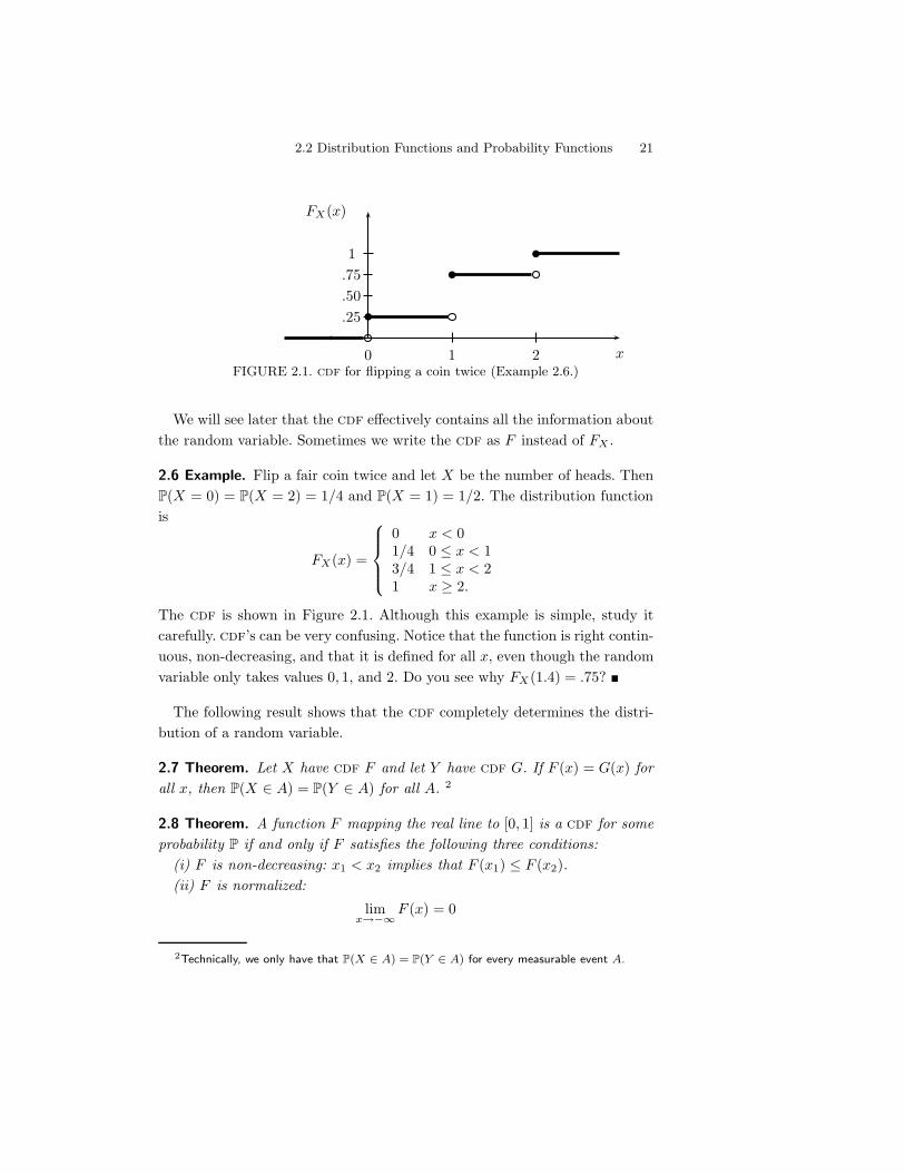
FIGURE 2.1. cdf for flipping a coin twice (Example 2.6.)
We will see later that the cdf e!ectively contains all the information aboutthe random variable. Sometimes we write the cdf as F instead of FX .
2.6 Example. Flip a fair coin twice and let X be the number of heads. ThenP(X = 0) = P(X = 2) = 1/4 and P(X = 1) = 1/2. The distribution functionis
FX(x) =
4556
557
0 x < 01/4 0 , x < 13/4 1 , x < 21 x * 2.
The cdf is shown in Figure 2.1. Although this example is simple, study itcarefully. cdf’s can be very confusing. Notice that the function is right contin-uous, non-decreasing, and that it is defined for all x, even though the randomvariable only takes values 0, 1, and 2. Do you see why FX(1.4) = .75? !
The following result shows that the cdf completely determines the distri-bution of a random variable.
2.7 Theorem. Let X have cdf F and let Y have cdf G. If F (x) = G(x) forall x, then P(X $ A) = P(Y $ A) for all A. 2
2.8 Theorem. A function F mapping the real line to [0, 1] is a cdf for someprobability P if and only if F satisfies the following three conditions:
(i) F is non-decreasing: x1 < x2 implies that F (x1) , F (x2).(ii) F is normalized:
limx"$!
F (x) = 0
2Technically, we only have that P(X ! A) = P(Y ! A) for every measurable event A.
22 2. Random Variables
andlim
x"!F (x) = 1.
(iii) F is right-continuous: F (x) = F (x+) for all x, where
F (x+) = limy!xy>x
F (y).
Proof. Suppose that F is a cdf. Let us show that (iii) holds. Let x bea real number and let y1, y2, . . . be a sequence of real numbers such thaty1 > y2 > · · · and limi yi = x. Let Ai = ("#, yi] and let A = ("#, x]. Notethat A =
%!i=1 Ai and also note that A1 ' A2 ' · · ·. Because the events are
monotone, limi P(Ai) = P(%
i Ai). Thus,
F (x) = P(A) = P($
i
Ai
)= lim
iP(Ai) = lim
iF (yi) = F (x+).
Showing (i) and (ii) is similar. Proving the other direction — namely, that ifF satisfies (i), (ii), and (iii) then it is a cdf for some random variable — usessome deep tools in analysis. !
2.9 Definition. X is discrete if it takes countably3many values{x1, x2, . . .}. We define the probability function or probability massfunction for X by fX(x) = P(X = x).
Thus, fX(x) * 0 for all x $ R and0
i fX(xi) = 1. Sometimes we write f
instead of fX . The cdf of X is related to fX by
FX(x) = P(X , x) =*
xi%x
fX(xi).
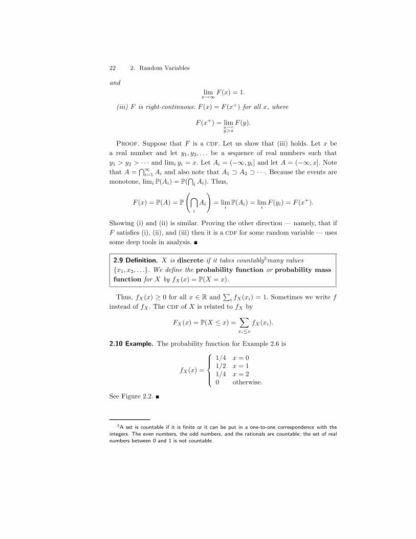
2.10 Example. The probability function for Example 2.6 is
fX(x) =
4556
557
1/4 x = 01/2 x = 11/4 x = 20 otherwise.
See Figure 2.2. !
3A set is countable if it is finite or it can be put in a one-to-one correspondence with theintegers. The even numbers, the odd numbers, and the rationals are countable; the set of realnumbers between 0 and 1 is not countable.
2.2 Distribution Functions and Probability Functions 23
0 1 2
1
fX(x)
x
.25.5.75
FIGURE 2.2. Probability function for flipping a coin twice (Example 2.6).
2.11 Definition. A random variable X is continuous if there exists afunction fX such that fX(x) * 0 for all x,
8!$! fX(x)dx = 1 and for
every a , b,
P(a < X < b) =9 b
afX(x)dx. (2.2)
The function fX is called the probability density function (pdf). Wehave that
FX(x) =9 x
$!fX(t)dt
and fX(x) = F &X(x) at all points x at which FX is di!erentiable.
Sometimes we write8
f(x)dx or8
f to mean8!$! f(x)dx.
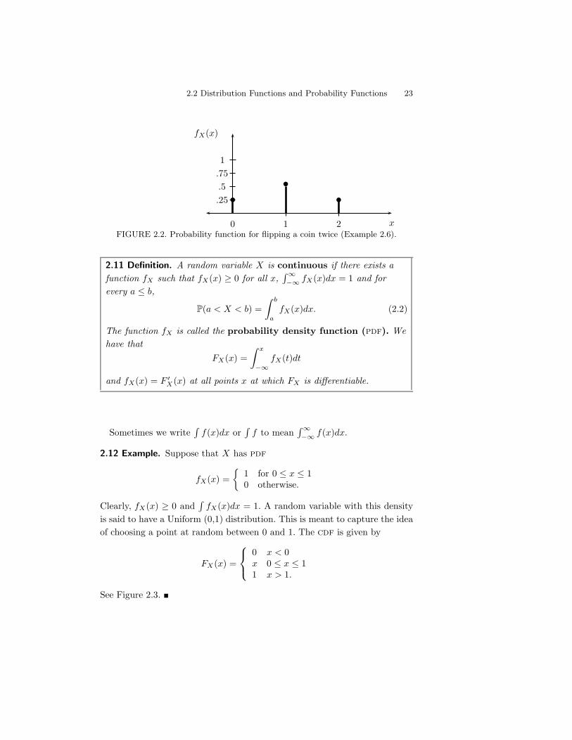
2.12 Example. Suppose that X has pdf
fX(x) ='
1 for 0 , x , 10 otherwise.
Clearly, fX(x) * 0 and8
fX(x)dx = 1. A random variable with this densityis said to have a Uniform (0,1) distribution. This is meant to capture the ideaof choosing a point at random between 0 and 1. The cdf is given by
FX(x) =
46
7
0 x < 0x 0 , x , 11 x > 1.
See Figure 2.3. !
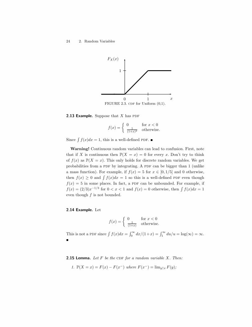
24 2. Random Variables
0 1
1
FX(x)
xFIGURE 2.3. cdf for Uniform (0,1).
2.13 Example. Suppose that X has pdf
f(x) ='
0 for x < 01
(1+x)2 otherwise.
Since8
f(x)dx = 1, this is a well-defined pdf. !
Warning! Continuous random variables can lead to confusion. First, notethat if X is continuous then P(X = x) = 0 for every x. Don’t try to thinkof f(x) as P(X = x). This only holds for discrete random variables. We getprobabilities from a pdf by integrating. A pdf can be bigger than 1 (unlikea mass function). For example, if f(x) = 5 for x $ [0, 1/5] and 0 otherwise,then f(x) * 0 and
8f(x)dx = 1 so this is a well-defined pdf even though
f(x) = 5 in some places. In fact, a pdf can be unbounded. For example, iff(x) = (2/3)x$1/3 for 0 < x < 1 and f(x) = 0 otherwise, then
8f(x)dx = 1
even though f is not bounded.
2.14 Example. Let
f(x) ='
0 for x < 01
(1+x) otherwise.
This is not a pdf since8
f(x)dx =8!0 dx/(1+x) =
8!1 du/u = log(#) =#.
!
2.15 Lemma. Let F be the cdf for a random variable X. Then:
1. P(X = x) = F (x)" F (x$) where F (x$) = limy'x F (y);
2.3 Some Important Discrete Random Variables 25
2. P(x < X , y) = F (y)" F (x);
3. P(X > x) = 1" F (x);
4. If X is continuous then
F (b)" F (a) = P(a < X < b) = P(a , X < b)
= P(a < X , b) = P(a , X , b).
It is also useful to define the inverse cdf (or quantile function).
2.16 Definition. Let X be a random variable with cdf F . The inverseCDF or quantile function is defined by4
F$1(q) = inf!x : F (x) > q
"
for q $ [0, 1]. If F is strictly increasing and continuous then F$1(q) is theunique real number x such that F (x) = q.
We call F$1(1/4) the first quartile, F$1(1/2) the median (or secondquartile), and F$1(3/4) the third quartile.
Two random variables X and Y are equal in distribution — writtenX
d= Y — if FX(x) = FY (x) for all x. This does not mean that X and Y areequal. Rather, it means that all probability statements about X and Y willbe the same. For example, suppose that P(X = 1) = P(X = "1) = 1/2. LetY = "X . Then P(Y = 1) = P(Y = "1) = 1/2 and so X
d= Y . But X and Y
are not equal. In fact, P(X = Y ) = 0.
2.3 Some Important Discrete Random Variables
Warning About Notation! It is traditional to write X ! F to indicatethat X has distribution F . This is unfortunate notation since the symbol !is also used to denote an approximation. The notation X ! F is so pervasivethat we are stuck with it. Read X ! F as “X has distribution F” not as “X
is approximately F”.
4If you are unfamiliar with “inf”, just think of it as the minimum.
26 2. Random Variables
The Point Mass Distribution. X has a point mass distribution at a,written X ! $a, if P(X = a) = 1 in which case
F (x) ='
0 x < a1 x * a.
The probability mass function is f(x) = 1 for x = a and 0 otherwise.
The Discrete Uniform Distribution. Let k > 1 be a given integer.Suppose that X has probability mass function given by
f(x) ='
1/k for x = 1, . . . , k0 otherwise.
We say that X has a uniform distribution on {1, . . . , k}.
The Bernoulli Distribution. Let X represent a binary coin flip. ThenP(X = 1) = p and P(X = 0) = 1" p for some p $ [0, 1]. We say that X has aBernoulli distribution written X ! Bernoulli(p). The probability function isf(x) = px(1" p)1$x for x $ {0, 1}.
The Binomial Distribution. Suppose we have a coin which falls headsup with probability p for some 0 , p , 1. Flip the coin n times and letX be the number of heads. Assume that the tosses are independent. Letf(x) = P(X = x) be the mass function. It can be shown that
f(x) =
: ;nx
<px(1 " p)n$x for x = 0, . . . , n
0 otherwise.
A random variable with this mass function is called a Binomial randomvariable and we write X ! Binomial(n, p). If X1 ! Binomial(n1, p) andX2 ! Binomial(n2, p) then X1 + X2 ! Binomial(n1 + n2, p).
Warning! Let us take this opportunity to prevent some confusion. X is arandom variable; x denotes a particular value of the random variable; n and p
are parameters, that is, fixed real numbers. The parameter p is usually un-known and must be estimated from data; that’s what statistical inference is allabout. In most statistical models, there are random variables and parameters:don’t confuse them.
The Geometric Distribution. X has a geometric distribution withparameter p $ (0, 1), written X ! Geom(p), if
P(X = k) = p(1" p)k$1, k * 1.
2.4 Some Important Continuous Random Variables 27
We have that!*
k=1
P(X = k) = p!*
k=1
(1 " p)k =p
1" (1 " p)= 1.
Think of X as the number of flips needed until the first head when flipping acoin.
The Poisson Distribution. X has a Poisson distribution with parameter%, written X ! Poisson(%) if
f(x) = e$!%x
x!x * 0.
Note that!*
x=0
f(x) = e$!!*
x=0
%x
x!= e$!e! = 1.
The Poisson is often used as a model for counts of rare events like radioactivedecay and tra#c accidents. If X1 ! Poisson(%1) and X2 ! Poisson(%2) thenX1 + X2 ! Poisson(%1 + %2).
Warning! We defined random variables to be mappings from a samplespace $ to R but we did not mention the sample space in any of the distri-butions above. As I mentioned earlier, the sample space often “disappears”but it is really there in the background. Let’s construct a sample space ex-plicitly for a Bernoulli random variable. Let $ = [0, 1] and define P to satisfyP([a, b]) = b" a for 0 , a , b , 1. Fix p $ [0, 1] and define
X(") ='
1 " , p0 " > p.
Then P(X = 1) = P(" , p) = P([0, p]) = p and P(X = 0) = 1 " p. Thus,X ! Bernoulli(p). We could do this for all the distributions defined above. Inpractice, we think of a random variable like a random number but formally itis a mapping defined on some sample space.
2.4 Some Important Continuous Random Variables
The Uniform Distribution. X has a Uniform(a, b) distribution, writtenX ! Uniform(a, b), if
f(x) ='
1b$a for x $ [a, b]0 otherwise
28 2. Random Variables
where a < b. The distribution function is
F (x) =
46
7
0 x < ax$ab$a x $ [a, b]1 x > b.
Normal (Gaussian). X has a Normal (or Gaussian) distribution withparameters µ and #, denoted by X ! N(µ,#2), if
f(x) =1
#/
2&exp'" 1
2#2(x" µ)2
2, x $ R (2.3)
where µ $ R and # > 0. The parameter µ is the “center” (or mean) of thedistribution and # is the “spread” (or standard deviation) of the distribu-tion. (The mean and standard deviation will be formally defined in the nextchapter.) The Normal plays an important role in probability and statistics.Many phenomena in nature have approximately Normal distributions. Later,we shall study the Central Limit Theorem which says that the distribution ofa sum of random variables can be approximated by a Normal distribution.
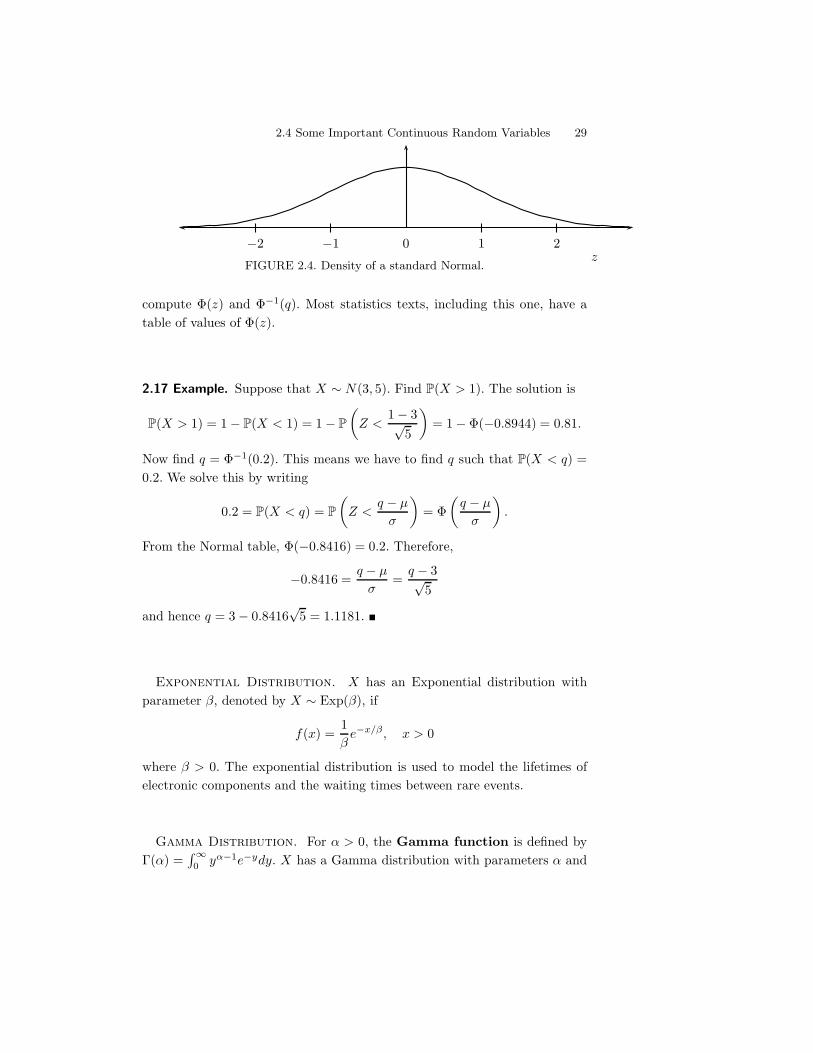
We say that X has a standard Normal distribution if µ = 0 and # = 1.Tradition dictates that a standard Normal random variable is denoted by Z.The pdf and cdf of a standard Normal are denoted by '(z) and %(z). Thepdf is plotted in Figure 2.4. There is no closed-form expression for %. Hereare some useful facts:
(i) If X ! N(µ,#2), then Z = (X " µ)/# ! N(0, 1).
(ii) If Z ! N(0, 1), then X = µ + #Z ! N(µ,#2).
(iii) If Xi ! N(µi,#2i ), i = 1, . . . , n are independent, then
n*
i=1
Xi ! N
(n*
i=1
µi,n*
i=1
#2i
).
It follows from (i) that if X ! N(µ,#2), then
P (a < X < b) = P-
a" µ
#< Z <
b" µ
#
.
= %-
b" µ
#
." %
-a" µ
#
..
Thus we can compute any probabilities we want as long as we can computethe cdf %(z) of a standard Normal. All statistical computing packages will
2.4 Some Important Continuous Random Variables 29
0 1 2"1"2z
FIGURE 2.4. Density of a standard Normal.
compute %(z) and %$1(q). Most statistics texts, including this one, have atable of values of %(z).
2.17 Example. Suppose that X ! N(3, 5). Find P(X > 1). The solution is
P(X > 1) = 1" P(X < 1) = 1" P-
Z <1" 3/
5
.= 1" %("0.8944) = 0.81.
Now find q = %$1(0.2). This means we have to find q such that P(X < q) =0.2. We solve this by writing
0.2 = P(X < q) = P-
Z <q " µ
#
.= %
-q " µ
#
..
From the Normal table, %("0.8416) = 0.2. Therefore,
"0.8416 =q " µ
#=
q " 3/5
and hence q = 3" 0.8416/
5 = 1.1181. !
Exponential Distribution. X has an Exponential distribution withparameter (, denoted by X ! Exp((), if
f(x) =1(
e$x/", x > 0
where ( > 0. The exponential distribution is used to model the lifetimes ofelectronic components and the waiting times between rare events.
Gamma Distribution. For ) > 0, the Gamma function is defined by&()) =
8!0 y#$1e$ydy. X has a Gamma distribution with parameters ) and
30 2. Random Variables
(, denoted by X ! Gamma(),(), if
f(x) =1
(#&())x#$1e$x/", x > 0
where ),( > 0. The exponential distribution is just a Gamma(1,() distribu-tion. If Xi ! Gamma()i,() are independent, then
0ni=1 Xi ! Gamma(
0ni=1 )i,().
The Beta Distribution. X has a Beta distribution with parameters) > 0 and ( > 0, denoted by X ! Beta(),(), if
f(x) =&()+ ()&())&(()
x#$1(1" x)"$1, 0 < x < 1.
t and Cauchy Distribution. X has a t distribution with * degrees offreedom — written X ! t$ — if
f(x) =&;$+12
<
&;$2
< 1;1 + x2
$
<($+1)/2.
The t distribution is similar to a Normal but it has thicker tails. In fact, theNormal corresponds to a t with * =#. The Cauchy distribution is a specialcase of the t distribution corresponding to * = 1. The density is
f(x) =1
&(1 + x2).
To see that this is indeed a density:9 !
$!f(x)dx =
1&
9 !
$!
dx
1 + x2=
1&
9 !
$!
d tan$1(x)dx
=1&
=tan$1(#) " tan$1("#)
>=
1&
?&2"+"&
2
,@= 1.
The !2 distribution. X has a !2 distribution with p degrees of freedom— written X ! !2
p — if
f(x) =1
&(p/2)2p/2x(p/2)$1e$x/2, x > 0.
If Z1, . . . , Zp are independent standard Normal random variables then0p
i=1 Z2i !
!2p.
2.5 Bivariate Distributions 31
2.5 Bivariate Distributions
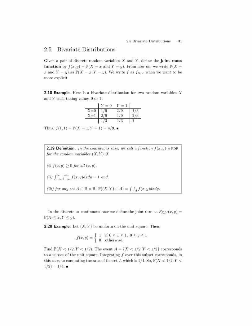
Given a pair of discrete random variables X and Y , define the joint massfunction by f(x, y) = P(X = x and Y = y). From now on, we write P(X =x and Y = y) as P(X = x, Y = y). We write f as fX,Y when we want to bemore explicit.
2.18 Example. Here is a bivariate distribution for two random variables X
and Y each taking values 0 or 1:
Y = 0 Y = 1X=0 1/9 2/9 1/3X=1 2/9 4/9 2/3
1/3 2/3 1
Thus, f(1, 1) = P(X = 1, Y = 1) = 4/9. !
2.19 Definition. In the continuous case, we call a function f(x, y) a pdf
for the random variables (X, Y ) if
(i) f(x, y) * 0 for all (x, y),
(ii)8!$!8!$! f(x, y)dxdy = 1 and,
(iii) for any set A & R- R, P((X, Y ) $ A) =8 8
A f(x, y)dxdy.
In the discrete or continuous case we define the joint cdf as FX,Y (x, y) =P(X , x, Y , y).
2.20 Example. Let (X, Y ) be uniform on the unit square. Then,
f(x, y) ='
1 if 0 , x , 1, 0 , y , 10 otherwise.
Find P(X < 1/2, Y < 1/2). The event A = {X < 1/2, Y < 1/2} correspondsto a subset of the unit square. Integrating f over this subset corresponds, inthis case, to computing the area of the set A which is 1/4. So, P(X < 1/2, Y <
1/2) = 1/4. !
32 2. Random Variables
2.21 Example. Let (X, Y ) have density
f(x, y) ='
x + y if 0 , x , 1, 0 , y , 10 otherwise.
Then9 1
0
9 1
0(x + y)dxdy =
9 1
0
A9 1
0xdx
Bdy +
9 1
0
A9 1
0y dx
Bdy
=9 1
0
12dy +
9 1
0y dy =
12
+12
= 1
which verifies that this is a pdf !
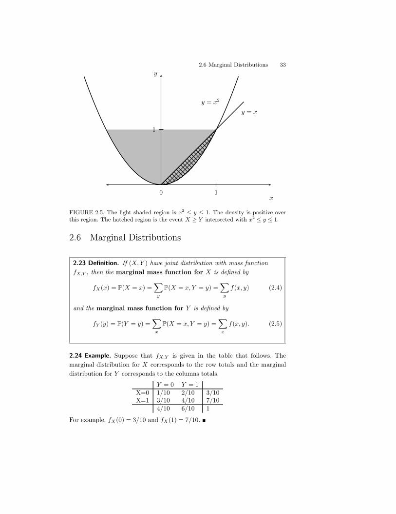
2.22 Example. If the distribution is defined over a non-rectangular region,then the calculations are a bit more complicated. Here is an example which Iborrowed from DeGroot and Schervish (2002). Let (X, Y ) have density
f(x, y) ='
c x2y if x2 , y , 10 otherwise.
Note first that "1 , x , 1. Now let us find the value of c. The trick here isto be careful about the range of integration. We pick one variable, x say, andlet it range over its values. Then, for each fixed value of x, we let y vary overits range, which is x2 , y , 1. It may help if you look at Figure 2.5. Thus,
1 =9 9
f(x, y)dydx = c
9 1
$1
9 1
x2x2y dy dx
= c
9 1
$1x2
A9 1
x2y dy
Bdx = c
9 1
$1x2 1" x4
2dx =
4c
21.
Hence, c = 21/4. Now let us compute P(X * Y ). This corresponds to the setA = {(x, y); 0 , x , 1, x2 , y , x}. (You can see this by drawing a diagram.)So,
P(X * Y ) =214
9 1
0
9 x
x2x2 y dy dx =
214
9 1
0x2
A9 x
x2y dy
Bdx
=214
9 1
0x2
-x2 " x4
2
.dx =
320
. !
2.6 Marginal Distributions 33
0 1
1
y = x2
y = x
x
y
FIGURE 2.5. The light shaded region is x2 " y " 1. The density is positive overthis region. The hatched region is the event X # Y intersected with x2 " y " 1.
2.6 Marginal Distributions
2.23 Definition. If (X, Y ) have joint distribution with mass functionfX,Y , then the marginal mass function for X is defined by
fX(x) = P(X = x) =*
y
P(X = x, Y = y) =*
y
f(x, y) (2.4)
and the marginal mass function for Y is defined by
fY (y) = P(Y = y) =*
x
P(X = x, Y = y) =*
x
f(x, y). (2.5)
2.24 Example. Suppose that fX,Y is given in the table that follows. Themarginal distribution for X corresponds to the row totals and the marginaldistribution for Y corresponds to the columns totals.
Y = 0 Y = 1X=0 1/10 2/10 3/10X=1 3/10 4/10 7/10
4/10 6/10 1
For example, fX(0) = 3/10 and fX(1) = 7/10. !
34 2. Random Variables
2.25 Definition. For continuous random variables, the marginal densitiesare
fX(x) =9
f(x, y)dy, and fY (y) =9
f(x, y)dx. (2.6)
The corresponding marginal distribution functions are denoted by FX andFY .
2.26 Example. Suppose that
fX,Y (x, y) = e$(x+y)
for x, y * 0. Then fX(x) = e$x8!0 e$ydy = e$x. !
2.27 Example. Suppose that
f(x, y) ='
x + y if 0 , x , 1, 0 , y , 10 otherwise.
Then
fY (y) =9 1
0(x + y) dx =
9 1
0xdx +
9 1
0y dx =
12
+ y. !
2.28 Example. Let (X, Y ) have density
f(x, y) ='
214 x2y if x2 , y , 10 otherwise.
Thus,
fX(x) =9
f(x, y)dy =214
x2
9 1
x2y dy =
218
x2(1" x4)
for "1 , x , 1 and fX(x) = 0 otherwise. !
2.7 Independent Random Variables
2.29 Definition. Two random variables X and Y are independent if,for every A and B,
P(X $ A, Y $ B) = P(X $ A)P(Y $ B) (2.7)
and we write X ! Y . Otherwise we say that X and Y are dependentand we write X !""""# Y .
2.7 Independent Random Variables 35
In principle, to check whether X and Y are independent we need to checkequation (2.7) for all subsets A and B. Fortunately, we have the followingresult which we state for continuous random variables though it is true fordiscrete random variables too.
2.30 Theorem. Let X and Y have joint pdf fX,Y . Then X ! Y if and onlyif fX,Y (x, y) = fX(x)fY (y) for all values x and y. 5
2.31 Example. Let X and Y have the following distribution:
Y = 0 Y = 1X=0 1/4 1/4 1/2X=1 1/4 1/4 1/2
1/2 1/2 1
Then, fX(0) = fX(1) = 1/2 and fY (0) = fY (1) = 1/2. X and Y are inde-pendent because fX(0)fY (0) = f(0, 0), fX(0)fY (1) = f(0, 1), fX(1)fY (0) =f(1, 0), fX(1)fY (1) = f(1, 1). Suppose instead that X and Y have the follow-ing distribution:
Y = 0 Y = 1X=0 1/2 0 1/2X=1 0 1/2 1/2
1/2 1/2 1
These are not independent because fX(0)fY (1) = (1/2)(1/2) = 1/4 yetf(0, 1) = 0. !
2.32 Example. Suppose that X and Y are independent and both have thesame density
f(x) ='
2x if 0 , x , 10 otherwise.
Let us find P(X + Y , 1). Using independence, the joint density is
f(x, y) = fX(x)fY (y) ='
4xy if 0 , x , 1, 0 , y , 10 otherwise.
5The statement is not rigorous because the density is defined only up to sets ofmeasure 0.
36 2. Random Variables
Now,
P(X + Y , 1) =9 9
x+y%1f(x, y)dydx
= 49 1
0x
A9 1$x
0ydy
Bdx
= 49 1
0x
(1 " x)2
2dx =
16. !
The following result is helpful for verifying independence.
2.33 Theorem. Suppose that the range of X and Y is a (possibly infinite)rectangle. If f(x, y) = g(x)h(y) for some functions g and h (not necessarilyprobability density functions) then X and Y are independent.
2.34 Example. Let X and Y have density
f(x, y) ='
2e$(x+2y) if x > 0 and y > 00 otherwise.
The range of X and Y is the rectangle (0,#)-(0,#). We can write f(x, y) =g(x)h(y) where g(x) = 2e$x and h(y) = e$2y. Thus, X ! Y . !
2.8 Conditional Distributions
If X and Y are discrete, then we can compute the conditional distribution ofX given that we have observed Y = y. Specifically, P(X = x|Y = y) = P(X =x, Y = y)/P(Y = y). This leads us to define the conditional probability massfunction as follows.
2.35 Definition. The conditional probability mass function is
fX|Y (x|y) = P(X = x|Y = y) =P(X = x, Y = y)
P(Y = y)=
fX,Y (x, y)fY (y)
if fY (y) > 0.
For continuous distributions we use the same definitions. 6 The interpre-tation di!ers: in the discrete case, fX|Y (x|y) is P(X = x|Y = y), but in thecontinuous case, we must integrate to get a probability.
6We are treading in deep water here. When we compute P(X $ A|Y = y) in thecontinuous case we are conditioning on the event {Y = y} which has probability 0. We
2.8 Conditional Distributions 37
2.36 Definition. For continuous random variables, the conditionalprobability density function is
fX|Y (x|y) =fX,Y (x, y)
fY (y)
assuming that fY (y) > 0. Then,
P(X $ A|Y = y) =9
AfX|Y (x|y)dx.
2.37 Example. Let X and Y have a joint uniform distribution on the unitsquare. Thus, fX|Y (x|y) = 1 for 0 , x , 1 and 0 otherwise. Given Y = y, X
is Uniform(0, 1). We can write this as X |Y = y ! Uniform(0, 1). !
From the definition of the conditional density, we see that fX,Y (x, y) =fX|Y (x|y)fY (y) = fY |X(y|x)fX(x). This can sometimes be useful as in exam-ple 2.39.
2.38 Example. Let
f(x, y) ='
x + y if 0 , x , 1, 0 , y , 10 otherwise.
Let us find P(X < 1/4|Y = 1/3). In example 2.27 we saw that fY (y) =y + (1/2). Hence,
fX|Y (x|y) =fX,Y (x, y)
fY (y)=
x + y
y + 12
.
So,
P
(X <
14
CCCCC Y =13
)=9 1/4
0fX|Y
(x
CCCCC13
)dx
=9 1/4
0
x + 13
13 + 1
2
dx =132 + 1
1213 + 1
2
=1180
. !
2.39 Example. Suppose that X ! Uniform(0, 1). After obtaining a value ofX we generate Y |X = x ! Uniform(x, 1). What is the marginal distribution
avoid this problem by defining things in terms of the pdf. The fact that this leads toa well-defined theory is proved in more advanced courses. Here, we simply take it as adefinition.
38 2. Random Variables
of Y ? First note that,
fX(x) ='
1 if 0 , x , 10 otherwise
andfY |X(y|x) =
'1
1$x if 0 < x < y < 10 otherwise.
So,
fX,Y (x, y) = fY |X(y|x)fX(x) ='
11$x if 0 < x < y < 10 otherwise.
The marginal for Y is
fY (y) =9 y
0fX,Y (x, y)dx =
9 y
0
dx
1" x= "
9 1$y
1
du
u= " log(1" y)
for 0 < y < 1. !
2.40 Example. Consider the density in Example 2.28. Let’s find fY |X(y|x).When X = x, y must satisfy x2 , y , 1. Earlier, we saw that fX(x) =(21/8)x2(1" x4). Hence, for x2 , y , 1,
fY |X(y|x) =f(x, y)fX(x)
=214 x2y
218 x2(1" x4)
=2y
1" x4.
Now let us compute P(Y * 3/4|X = 1/2). This can be done by first notingthat fY |X(y|1/2) = 32y/15. Thus,
P(Y * 3/4|X = 1/2) =9 1
3/4f(y|1/2)dy =
9 1
3/4
32y
15dy =
715
. !
2.9 Multivariate Distributions and iid Samples
Let X = (X1, . . . , Xn) where X1, . . . , Xn are random variables. We call X arandom vector. Let f(x1, . . . , xn) denote the pdf. It is possible to definetheir marginals, conditionals etc. much the same way as in the bivariate case.We say that X1, . . . , Xn are independent if, for every A1, . . . , An,
P(X1 $ A1, . . . , Xn $ An) =n/
i=1
P(Xi $ Ai). (2.8)
It su#ces to check that f(x1, . . . , xn) =Dn
i=1 fXi(xi).
2.10 Two Important Multivariate Distributions 39
2.41 Definition. If X1, . . . , Xn are independent and each has the samemarginal distribution with cdf F , we say that X1, . . . , Xn are iid
(independent and identically distributed) and we write
X1, . . .Xn ! F.
If F has density f we also write X1, . . . Xn ! f . We also call X1, . . . , Xn
a random sample of size n from F .
Much of statistical theory and practice begins with iid observations and weshall study this case in detail when we discuss statistics.
2.10 Two Important Multivariate Distributions
Multinomial. The multivariate version of a Binomial is called a Multino-mial. Consider drawing a ball from an urn which has balls with k di!erentcolors labeled “color 1, color 2, . . . , color k.” Let p = (p1, . . . , pk) wherepj * 0 and
0kj=1 pj = 1 and suppose that pj is the probability of drawing
a ball of color j. Draw n times (independent draws with replacement) andlet X = (X1, . . . , Xk) where Xj is the number of times that color j appears.Hence, n =
0kj=1 Xj . We say that X has a Multinomial (n,p) distribution
written X !Multinomial(n, p). The probability function is
f(x) =-
n
x1 . . . xk
.px11 · · · pxk
k (2.9)
where -n
x1 . . . xk
.=
n!x1! · · ·xk!
.
2.42 Lemma. Suppose that X ! Multinomial(n, p) where X = (X1, . . . , Xk)and p = (p1, . . . , pk). The marginal distribution of Xj is Binomial (n,pj).
Multivariate Normal. The univariate Normal has two parameters, µ
and #. In the multivariate version, µ is a vector and # is replaced by a matrix'. To begin, let
Z =
E
FGZ1...
Zk
H
IJ
40 2. Random Variables
where Z1, . . . , Zk ! N(0, 1) are independent. The density of Z is 7
f(z) =k/
i=1
f(zi) =1
(2&)k/2exp
46
7"12
k*
j=1
z2j
KL
M
=1
(2&)k/2exp'"1
2zT z
2.
We say that Z has a standard multivariate Normal distribution written Z !N(0, I) where it is understood that 0 represents a vector of k zeroes and I isthe k - k identity matrix.
More generally, a vector X has a multivariate Normal distribution, denotedby X ! N(µ,'), if it has density 8
f(x; µ,') =1
(2&)k/2|(')|1/2exp'"1
2(x" µ)T'$1(x" µ)
2(2.10)
where |'| denotes the determinant of ', µ is a vector of length k and ' is ak - k symmetric, positive definite matrix. 9 Setting µ = 0 and ' = I givesback the standard Normal.
Since ' is symmetric and positive definite, it can be shown that there existsa matrix '1/2 — called the square root of ' — with the following properties:(i) '1/2 is symmetric, (ii) ' = '1/2'1/2 and (iii) '1/2'$1/2 = '$1/2'1/2 = I
where '$1/2 = ('1/2)$1.
2.43 Theorem. If Z ! N(0, I) and X = µ + '1/2Z then X ! N(µ,').Conversely, if X ! N(µ,'), then '$1/2(X " µ) ! N(0, I).
Suppose we partition a random Normal vector X as X = (Xa, Xb) We cansimilarly partition µ = (µa, µb) and
' =-
'aa 'ab
'ba 'bb
..
2.44 Theorem. Let X ! N(µ,'). Then:(1) The marginal distribution of Xa is Xa ! N(µa,'aa).(2) The conditional distribution of Xb given Xa = xa is
Xb|Xa = xa ! N;
µb + 'ba'$1aa (xa " µa), 'bb " 'ba'$1
aa 'ab
<.
(3) If a is a vector then aT X ! N(aT µ, aT'a).(4) V = (X " µ)T'$1(X " µ) ! !2
k.
7If a and b are vectors then aT b =0k
i=1 aibi.8!!1 is the inverse of the matrix !.9A matrix ! is positive definite if, for all nonzero vectors x, xT!x > 0.
2.11 Transformations of Random Variables 41
2.11 Transformations of Random Variables
Suppose that X is a random variable with pdf fX and cdf FX . Let Y = r(X)be a function of X , for example, Y = X2 or Y = eX . We call Y = r(X) atransformation of X . How do we compute the pdf and cdf of Y ? In thediscrete case, the answer is easy. The mass function of Y is given by
fY (y) = P(Y = y) = P(r(X) = y)
= P({x; r(x) = y}) = P(X $ r$1(y)).
2.45 Example. Suppose that P(X = "1) = P(X = 1) = 1/4 and P(X = 0) =1/2. Let Y = X2. Then, P(Y = 0) = P(X = 0) = 1/2 and P(Y = 1) = P(X =1) + P(X = "1) = 1/2. Summarizing:
x fX(x)-1 1/40 1/21 1/4
y fY (y)0 1/21 1/2
Y takes fewer values than X because the transformation is not one-to-one. !
The continuous case is harder. There are three steps for finding fY :
Three Steps for Transformations
1. For each y, find the set Ay = {x : r(x) , y}.
2. Find the cdf
FY (y) = P(Y , y) = P(r(X) , y)
= P({x; r(x) , y})
=9
Ay
fX(x)dx. (2.11)
3. The pdf is fY (y) = F &Y (y).
2.46 Example. Let fX(x) = e$x for x > 0. Hence, FX(x) =8 x0 fX(s)ds =
1" e$x. Let Y = r(X) = log X . Then, Ay = {x : x , ey} and
FY (y) = P(Y , y) = P(log X , y)
= P(X , ey) = FX(ey) = 1" e$ey
.
Therefore, fY (y) = eye$eyfor y $ R. !
42 2. Random Variables
2.47 Example. Let X ! Uniform("1, 3). Find the pdf of Y = X2. Thedensity of X is
fX(x) ='
1/4 if " 1 < x < 30 otherwise.
Y can only take values in (0, 9). Consider two cases: (i) 0 < y < 1 and (ii) 1 ,y < 9. For case (i), Ay = ["/y,
/y] and FY (y) =
8Ay
fX(x)dx = (1/2)/y.For case (ii), Ay = ["1,
/y] and FY (y) =
8Ay
fX(x)dx = (1/4)(/y + 1).Di!erentiating F we get
fY (y) =
4556
557
14(
y if 0 < y < 11
8(
y if 1 < y < 9
0 otherwise. !
When r is strictly monotone increasing or strictly monotone decreasing thenr has an inverse s = r$1 and in this case one can show that
fY (y) = fX(s(y))CCCCds(y)dy
CCCC . (2.12)
2.12 Transformations of Several Random Variables
In some cases we are interested in transformations of several random variables.For example, if X and Y are given random variables, we might want to knowthe distribution of X/Y , X + Y , max{X, Y } or min{X, Y }. Let Z = r(X, Y )be the function of interest. The steps for finding fZ are the same as before:
Three Steps for Transformations
1. For each z, find the set Az = {(x, y) : r(x, y) , z}.
2. Find the cdf
FZ(z) = P(Z , z) = P(r(X, Y ) , z)
= P({(x, y); r(x, y) , z}) =9 9
Az
fX,Y (x, y) dx dy.
3. Then fZ(z) = F &Z(z).
2.13 Appendix 43
2.48 Example. Let X1, X2 ! Uniform(0, 1) be independent. Find the densityof Y = X1 + X2. The joint density of (X1, X2) is
f(x1, x2) ='
1 0 < x1 < 1, 0 < x2 < 10 otherwise.
Let r(x1, x2) = x1 + x2. Now,
FY (y) = P(Y , y) = P(r(X1, X2) , y)
= P({(x1, x2) : r(x1, x2) , y}) =9 9
Ay
f(x1, x2)dx1dx2.
Now comes the hard part: finding Ay. First suppose that 0 < y , 1. Then Ay
is the triangle with vertices (0, 0), (y, 0) and (0, y). See Figure 2.6. In this case,8 8Ay
f(x1, x2)dx1dx2 is the area of this triangle which is y2/2. If 1 < y < 2,then Ay is everything in the unit square except the triangle with vertices(1, y " 1), (1, 1), (y " 1, 1). This set has area 1" (2" y)2/2. Therefore,
FY (y) =
455556
55557
0 y < 0y2
2 0 , y < 1
1" (2$y)2
2 1 , y < 2
1 y * 2.
By di!erentiation, the pdf is
fY (y) =
456
57
y 0 , y , 12" y 1 , y , 2
0 otherwise. !
2.13 Appendix
Recall that a probability measure P is defined on a #-field A of a samplespace $. A random variable X is a measurable map X : $) R. Measurablemeans that, for every x, {" : X(") , x} $ A.
2.14 Exercises
1. Show thatP(X = x) = F (x+)" F (x$).
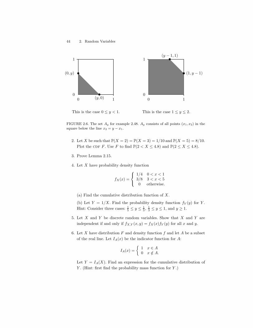
44 2. Random Variables
0 10
1
(0, y)
(y, 0)
This is the case 0 , y < 1.
0 10
1
(1, y " 1)
(y " 1, 1)
This is the case 1 , y , 2.
FIGURE 2.6. The set Ay for example 2.48. Ay consists of all points (x1, x2) in thesquare below the line x2 = y % x1.
2. Let X be such that P(X = 2) = P(X = 3) = 1/10 and P(X = 5) = 8/10.Plot the cdf F . Use F to find P(2 < X , 4.8) and P(2 , X , 4.8).
3. Prove Lemma 2.15.
4. Let X have probability density function
fX(x) =
46
7
1/4 0 < x < 13/8 3 < x < 50 otherwise.
(a) Find the cumulative distribution function of X .
(b) Let Y = 1/X . Find the probability density function fY (y) for Y .Hint: Consider three cases: 1
5 , y , 13 , 1
3 , y , 1, and y * 1.
5. Let X and Y be discrete random variables. Show that X and Y areindependent if and only if fX,Y (x, y) = fX(x)fY (y) for all x and y.
6. Let X have distribution F and density function f and let A be a subsetof the real line. Let IA(x) be the indicator function for A:
IA(x) ='
1 x $ A0 x /$ A.
Let Y = IA(X). Find an expression for the cumulative distribution ofY . (Hint: first find the probability mass function for Y .)
2.14 Exercises 45
7. Let X and Y be independent and suppose that each has a Uniform(0, 1)distribution. Let Z = min{X, Y }. Find the density fZ(z) for Z. Hint:It might be easier to first find P(Z > z).
8. Let X have cdf F . Find the cdf of X+ = max{0, X}.
9. Let X ! Exp((). Find F (x) and F$1(q).
10. Let X and Y be independent. Show that g(X) is independent of h(Y )where g and h are functions.
11. Suppose we toss a coin once and let p be the probability of heads. LetX denote the number of heads and let Y denote the number of tails.
(a) Prove that X and Y are dependent.
(b) Let N ! Poisson(%) and suppose we toss a coin N times. Let X andY be the number of heads and tails. Show that X and Y are independent.
12. Prove Theorem 2.33.
13. Let X ! N(0, 1) and let Y = eX .
(a) Find the pdf for Y . Plot it.
(b) (Computer Experiment.) Generate a vector x = (x1, . . . , x10,000) con-sisting of 10,000 random standard Normals. Let y = (y1, . . . , y10,000)where yi = exi . Draw a histogram of y and compare it to the pdf youfound in part (a).
14. Let (X, Y ) be uniformly distributed on the unit disk {(x, y) : x2 + y2 ,1}. Let R =
/X2 + Y 2. Find the cdf and pdf of R.
15. (A universal random number generator.) Let X have a continuous, strictlyincreasing cdf F . Let Y = F (X). Find the density of Y . This is calledthe probability integral transform. Now let U ! Uniform(0, 1) and letX = F$1(U). Show that X ! F . Now write a program that takesUniform (0,1) random variables and generates random variables froman Exponential (() distribution.
16. Let X ! Poisson(%) and Y ! Poisson(µ) and assume that X and Y areindependent. Show that the distribution of X given that X + Y = n isBinomial(n,&) where & = %/(%+ µ).
46 2. Random Variables
Hint 1: You may use the following fact: If X ! Poisson(%) and Y !Poisson(µ), and X and Y are independent, then X+Y ! Poisson(µ+%).
Hint 2: Note that {X = x, X + Y = n} = {X = x, Y = n" x}.
17. LetfX,Y (x, y) =
'c(x + y2) 0 , x , 1 and 0 , y , 10 otherwise.
Find P;X < 1
2 | Y = 12
<.
18. Let X ! N(3, 16). Solve the following using the Normal table and usinga computer package.
(a) Find P(X < 7).
(b) Find P(X > "2).
(c) Find x such that P(X > x) = .05.
(d) Find P(0 , X < 4).
(e) Find x such that P(|X | > |x|) = .05.
19. Prove formula (2.12).
20. Let X, Y ! Uniform(0, 1) be independent. Find the pdf for X " Y andX/Y .
21. Let X1, . . . , Xn ! Exp(() be iid. Let Y = max{X1, . . . , Xn}. Find thepdf of Y . Hint: Y , y if and only if Xi , y for i = 1, . . . , n.
This is page 47Printer: Opaque this
3Expectation
3.1 Expectation of a Random Variable
The mean, or expectation, of a random variable X is the average value of X .
3.1 Definition. The expected value, or mean, or first moment, ofX is defined to be
E(X) =9
xdF (x) =
: 0x xf(x) if X is discrete
8xf(x)dx if X is continuous
(3.1)
assuming that the sum (or integral) is well defined. We use the followingnotation to denote the expected value of X:
E(X) = EX =9
xdF (x) = µ = µX . (3.2)
The expectation is a one-number summary of the distribution. Think ofE(X) as the average
0ni=1 Xi/n of a large number of iid draws X1, . . . , Xn.
The fact that E(X) .0n
i=1 Xi/n is actually more than a heuristic; it is atheorem called the law of large numbers that we will discuss in Chapter 5.
The notation8
xdF (x) deserves some comment. We use it merely as aconvenient unifying notation so we don’t have to write
0x xf(x) for discrete
48 3. Expectation
random variables and8
xf(x)dx for continuous random variables, but youshould be aware that
8xdF (x) has a precise meaning that is discussed in real
analysis courses.To ensure that E(X) is well defined, we say that E(X) exists if
8x |x|dFX (x) <
#. Otherwise we say that the expectation does not exist.
3.2 Example. Let X ! Bernoulli(p). Then E(X) =01
x=0 xf(x) = (0 - (1 "p)) + (1- p) = p. !
3.3 Example. Flip a fair coin two times. Let X be the number of heads. Then,E(X) =
8xdFX (x) =
0x xfX(x) = (0 - f(0)) + (1 - f(1)) + (2 - f(2)) =
(0- (1/4)) + (1- (1/2)) + (2- (1/4)) = 1. !
3.4 Example. Let X ! Uniform("1, 3). Then, E(X) =8
xdFX(x) =8
xfX(x)dx =14
8 3$1 xdx = 1. !
3.5 Example. Recall that a random variable has a Cauchy distribution if ithas density fX(x) = {&(1 + x2)}$1. Using integration by parts, (set u = x
and v = tan$1 x),9
|x|dF (x) =2&
9 !
0
xdx
1 + x2==x tan$1(x)
>!0"9 !
0tan$1 xdx =#
so the mean does not exist. If you simulate a Cauchy distribution many timesand take the average, you will see that the average never settles down. Thisis because the Cauchy has thick tails and hence extreme observations arecommon. !
From now on, whenever we discuss expectations, we implicitly assume thatthey exist.
Let Y = r(X). How do we compute E(Y )? One way is to find fY (y) andthen compute E(Y ) =
8yfY (y)dy. But there is an easier way.
3.6 Theorem (The Rule of the Lazy Statistician). Let Y = r(X). Then
E(Y ) = E(r(X)) =9
r(x)dFX (x). (3.3)
This result makes intuitive sense. Think of playing a game where we drawX at random and then I pay you Y = r(X). Your average income is r(x) timesthe chance that X = x, summed (or integrated) over all values of x. Here is
3.1 Expectation of a Random Variable 49
a special case. Let A be an event and let r(x) = IA(x) where IA(x) = 1 ifx $ A and IA(x) = 0 if x /$ A. Then
E(IA(X)) =9
IA(x)fX(x)dx =9
AfX(x)dx = P(X $ A).
In other words, probability is a special case of expectation.
3.7 Example. Let X ! Unif(0, 1). Let Y = r(X) = eX . Then,
E(Y ) =9 1
0exf(x)dx =
9 1
0exdx = e" 1.
Alternatively, you could find fY (y) which turns out to be fY (y) = 1/y for1 < y < e. Then, E(Y ) =
8 e1 y f(y)dy = e" 1. !
3.8 Example. Take a stick of unit length and break it at random. Let Y bethe length of the longer piece. What is the mean of Y ? If X is the break pointthen X ! Unif(0, 1) and Y = r(X) = max{X, 1 " X}. Thus, r(x) = 1 " x
when 0 < x < 1/2 and r(x) = x when 1/2 , x < 1. Hence,
E(Y ) =9
r(x)dF (x) =9 1/2
0(1" x)dx +
9 1
1/2xdx =
34. !
Functions of several variables are handled in a similar way. If Z = r(X, Y )then
E(Z) = E(r(X, Y )) =9 9
r(x, y)dF (x, y). (3.4)
3.9 Example. Let (X, Y ) have a jointly uniform distribution on the unitsquare. Let Z = r(X, Y ) = X2 + Y 2. Then,
E(Z) =9 9
r(x, y)dF (x, y) =9 1
0
9 1
0(x2 + y2) dxdy
=9 1
0x2 dx +
9 1
0y2 dy =
23. !
The kth moment of X is defined to be E(Xk) assuming that E(|X |k) <#.
3.10 Theorem. If the kth moment exists and if j < k then the jth momentexists.
Proof. We have
E|X |j =9 !
$!|x|jfX(x)dx
50 3. Expectation
=9
|x|%1|x|jfX(x)dx +
9
|x|>1|x|jfX(x)dx
,9
|x|%1fX(x)dx +
9
|x|>1|x|kfX(x)dx
, 1 + E(|X |k) <#. !
The kth central moment is defined to be E((X " µ)k).
3.2 Properties of Expectations
3.11 Theorem. If X1, . . . , Xn are random variables and a1, . . . , an are con-stants, then
E(*
i
aiXi
)=*
i
aiE(Xi). (3.5)
3.12 Example. Let X ! Binomial(n, p). What is the mean of X? We couldtry to appeal to the definition:
E(X) =9
xdFX(x) =*
x
xfX(x) =n*
x=0
x
-n
x
.px(1" p)n$x
but this is not an easy sum to evaluate. Instead, note that X =0n
i=1 Xi
where Xi = 1 if the ith toss is heads and Xi = 0 otherwise. Then E(Xi) =(p- 1) + ((1" p)- 0) = p and E(X) = E(
0i Xi) =
0i E(Xi) = np. !
3.13 Theorem. Let X1, . . . , Xn be independent random variables. Then,
E(
n/
i=1
Xi
)=/
i
E(Xi). (3.6)
Notice that the summation rule does not require independence but themultiplication rule does.
3.3 Variance and Covariance
The variance measures the “spread” of a distribution. 1
1We can’t use E(X " µ) as a measure of spread since E(X " µ) = E(X) " µ = µ " µ = 0.We can and sometimes do use E|X " µ| as a measure of spread but more often we use thevariance.
3.3 Variance and Covariance 51
3.14 Definition. Let X be a random variable with mean µ. The varianceof X — denoted by #2 or #2
X or V(X) or VX — is defined by
#2 = E(X " µ)2 =9
(x" µ)2dF (x) (3.7)
assuming this expectation exists. The standard deviation issd(X) =
3V(X) and is also denoted by # and #X .
3.15 Theorem. Assuming the variance is well defined, it has the followingproperties:
1. V(X) = E(X2)" µ2.
2. If a and b are constants then V(aX + b) = a2V(X).
3. If X1, . . . , Xn are independent and a1, . . . , an are constants, then
V(
n*
i=1
aiXi
)=
n*
i=1
a2i V(Xi). (3.8)
3.16 Example. Let X ! Binomial(n, p). We write X =0
i Xi where Xi = 1if toss i is heads and Xi = 0 otherwise. Then X =
0i Xi and the random
variables are independent. Also, P(Xi = 1) = p and P(Xi = 0) = 1"p. Recallthat
E(Xi) =-
p- 1.
+-
(1" p)- 0.
= p.
Now,
E(X2i ) =
-p- 12
.+-
(1" p)- 02
.= p.
Therefore, V(Xi) = E(X2i ) " p2 = p " p2 = p(1 " p). Finally, V(X) =
V(0
i Xi) =0
i V(Xi) =0
i p(1 " p) = np(1 " p). Notice that V(X) = 0if p = 1 or p = 0. Make sure you see why this makes intuitive sense. !
If X1, . . . , Xn are random variables then we define the sample mean to be
Xn =1n
n*
i=1
Xi (3.9)
and the sample variance to be
S2n =
1n" 1
n*
i=1
;Xi "Xn
<2. (3.10)
52 3. Expectation
3.17 Theorem. Let X1, . . . , Xn be iid and let µ = E(Xi), #2 = V(Xi). Then
E(Xn) = µ, V(Xn) =#2
nand E(S2
n) = #2.
If X and Y are random variables, then the covariance and correlation be-tween X and Y measure how strong the linear relationship is between X andY .
3.18 Definition. Let X and Y be random variables with means µX andµY and standard deviations #X and #Y . Define the covariance betweenX and Y by
Cov(X, Y ) = E-
(X " µX)(Y " µY ).
(3.11)
and the correlation by
+ = +X,Y = +(X, Y ) =Cov(X, Y )#X#Y
. (3.12)
3.19 Theorem. The covariance satisfies:
Cov(X, Y ) = E(XY )" E(X)E(Y ).
The correlation satisfies:
"1 , +(X, Y ) , 1.
If Y = aX + b for some constants a and b then +(X, Y ) = 1 if a > 0 and+(X, Y ) = "1 if a < 0. If X and Y are independent, then Cov(X, Y ) = + = 0.The converse is not true in general.
3.20 Theorem. V(X + Y ) = V(X) + V(Y ) + 2Cov(X, Y ) and V(X " Y ) =V(X)+V(Y )"2Cov(X, Y ). More generally, for random variables X1, . . . , Xn,
V(*
i
aiXi
)=*
i
a2i V(Xi) + 2
**
i<j
aiajCov(Xi, Xj).
3.4 Expectation and Variance of Important RandomVariables
Here we record the expectation of some important random variables:
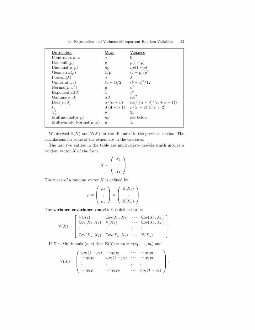
3.4 Expectation and Variance of Important Random Variables 53
Distribution Mean VariancePoint mass at a a 0Bernoulli(p) p p(1" p)Binomial(n, p) np np(1" p)Geometric(p) 1/p (1" p)/p2
Poisson(%) % %Uniform(a, b) (a + b)/2 (b " a)2/12Normal(µ,#2) µ #2
Exponential(() ( (2
Gamma(),() )( )(2
Beta(),() )/()+ () )(/(() + ()2()+ ( + 1))t$ 0 (if * > 1) */(* " 2) (if * > 2)!2
p p 2pMultinomial(n, p) np see belowMultivariate Normal(µ,') µ '
We derived E(X) and V(X) for the Binomial in the previous section. Thecalculations for some of the others are in the exercises.
The last two entries in the table are multivariate models which involve arandom vector X of the form
X =
E
FGX1...
Xk
H
IJ .
The mean of a random vector X is defined by
µ =
E
FGµ1...
µk
H
IJ =
E
FGE(X1)
...E(Xk)
H
IJ .
The variance-covariance matrix ' is defined to be
V(X) =
N
OOOP
V(X1) Cov(X1, X2) · · · Cov(X1, Xk)Cov(X2, X1) V(X2) · · · Cov(X2, Xk)...
......
...Cov(Xk, X1) Cov(Xk, X2) · · · V(Xk)
Q
RRRS.
If X ! Multinomial(n, p) then E(X) = np = n(p1, . . . , pk) and
V(X) =
E
FFFG
np1(1" p1) "np1p2 · · · "np1pk
"np2p1 np2(1" p2) · · · "np2pk...
......
..."npkp1 "npkp2 · · · npk(1" pk)
H
IIIJ.
54 3. Expectation
To see this, note that the marginal distribution of any one component of thevector Xi ! Binomial(n, pi). Thus, E(Xi) = npi and V(Xi) = npi(1 " pi).Note also that Xi + Xj ! Binomial(n, pi + pj). Thus, V(Xi + Xj) = n(pi +pj)(1 " [pi + pj ]). On the other hand, using the formula for the varianceof a sum, we have that V(Xi + Xj) = V(Xi) + V(Xj) + 2Cov(Xi, Xj) =npi(1 " pi) + npj(1 " pj) + 2Cov(Xi, Xj). If we equate this formula withn(pi + pj)(1" [pi + pj ]) and solve, we get Cov(Xi, Xj) = "npipj.
Finally, here is a lemma that can be useful for finding means and variancesof linear combinations of multivariate random vectors.
3.21 Lemma. If a is a vector and X is a random vector with mean µ andvariance ', then E(aT X) = aT µ and V(aT X) = aT'a. If A is a matrix thenE(AX) = Aµ and V(AX) = A'AT .
3.5 Conditional Expectation
Suppose that X and Y are random variables. What is the mean of X amongthose times when Y = y? The answer is that we compute the mean of X asbefore but we substitute fX|Y (x|y) for fX(x) in the definition of expectation.
3.22 Definition. The conditional expectation of X given Y = y is
E(X |Y = y) =
: 0x fX|Y (x|y) dx discrete case
8x fX|Y (x|y) dx continuous case.
(3.13)
If r(x, y) is a function of x and y then
E(r(X, Y )|Y = y) =
: 0r(x, y) fX|Y (x|y) dx discrete case
8r(x, y) fX|Y (x|y) dx continuous case.
(3.14)
Warning! Here is a subtle point. Whereas E(X) is a number, E(X |Y = y)is a function of y. Before we observe Y , we don’t know the value of E(X |Y = y)so it is a random variable which we denote E(X |Y ). In other words, E(X |Y )is the random variable whose value is E(X |Y = y) when Y = y. Similarly,E(r(X, Y )|Y ) is the random variable whose value is E(r(X, Y )|Y = y) whenY = y. This is a very confusing point so let us look at an example.
3.23 Example. Suppose we draw X ! Unif(0, 1). After we observe X = x,we draw Y |X = x ! Unif(x, 1). Intuitively, we expect that E(Y |X = x) =
3.5 Conditional Expectation 55
(1 + x)/2. In fact, fY |X(y|x) = 1/(1" x) for x < y < 1 and
E(Y |X = x) =9 1
xy fY |X(y|x)dy =
11" x
9 1
xy dy =
1 + x
2
as expected. Thus, E(Y |X) = (1 + X)/2. Notice that E(Y |X) = (1 + X)/2 isa random variable whose value is the number E(Y |X = x) = (1 + x)/2 onceX = x is observed. !
3.24 Theorem (The Rule of Iterated Expectations). For random variables X
and Y , assuming the expectations exist, we have that
E [E(Y |X)] = E(Y ) and E [E(X |Y )] = E(X). (3.15)
More generally, for any function r(x, y) we have
E [E(r(X, Y )|X)] = E(r(X, Y )). (3.16)
Proof. We’ll prove the first equation. Using the definition of conditionalexpectation and the fact that f(x, y) = f(x)f(y|x),
E [E(Y |X)] =9
E(Y |X = x)fX(x)dx =9 9
yf(y|x)dyf(x)dx
=9 9
yf(y|x)f(x)dxdy =9 9
yf(x, y)dxdy = E(Y ). !
3.25 Example. Consider example 3.23. How can we compute E(Y )? Onemethod is to find the joint density f(x, y) and then compute E(Y ) =
8 8yf(x, y)dxdy.
An easier way is to do this in two steps. First, we already know that E(Y |X) =(1 + X)/2. Thus,
E(Y ) = EE(Y |X) = E-
(1 + X)2
.
=(1 + E(X))
2=
(1 + (1/2))2
= 3/4. !
3.26 Definition. The conditional variance is defined as
V(Y |X = x) =9
(y " µ(x))2f(y|x)dy (3.17)
where µ(x) = E(Y |X = x).
3.27 Theorem. For random variables X and Y ,
V(Y ) = EV(Y |X) + VE(Y |X).
56 3. Expectation
3.28 Example. Draw a county at random from the United States. Then drawn people at random from the county. Let X be the number of those peoplewho have a certain disease. If Q denotes the proportion of people in thatcounty with the disease, then Q is also a random variable since it varies fromcounty to county. Given Q = q, we have that X ! Binomial(n, q). Thus,E(X |Q = q) = nq and V(X |Q = q) = nq(1 " q). Suppose that the randomvariable Q has a Uniform (0,1) distribution. A distribution that is constructedin stages like this is called a hierarchical model and can be written as
Q ! Uniform(0, 1)
X |Q = q ! Binomial(n, q).
Now, E(X) = EE(X |Q) = E(nQ) = nE(Q) = n/2. Let us compute thevariance of X . Now, V(X) = EV(X |Q) + VE(X |Q). Let’s compute thesetwo terms. First, EV(X |Q) = E[nQ(1 " Q)] = nE(Q(1 " Q)) = n
8q(1 "
q)f(q)dq = n8 10 q(1 " q)dq = n/6. Next, VE(X |Q) = V(nQ) = n2V(Q) =
n28(q " (1/2))2dq = n2/12. Hence, V(X) = (n/6) + (n2/12). !
3.6 Moment Generating Functions
Now we will define the moment generating function which is used for findingmoments, for finding the distribution of sums of random variables and whichis also used in the proofs of some theorems.
3.29 Definition. The moment generating function mgf, or Laplacetransform, of X is defined by
,X(t) = E(etX) =9
etxdF (x)
where t varies over the real numbers.
In what follows, we assume that the mgf is well defined for all t in someopen interval around t = 0. 2
When the mgf is well defined, it can be shown that we can interchange theoperations of di!erentiation and “taking expectation.” This leads to
,&(0) =A
d
dtEetX
B
t=0
= EA
d
dtetX
B
t=0
= E=XetX
>t=0
= E(X).
2A related function is the characteristic function, defined by E(eitX) where i =#"1. This
function is always well defined for all t.
3.6 Moment Generating Functions 57
By taking k derivatives we conclude that ,(k)(0) = E(Xk). This gives us amethod for computing the moments of a distribution.
3.30 Example. Let X ! Exp(1). For any t < 1,
,X(t) = EetX =9 !
0etxe$xdx =
9 !
0e(t$1)xdx =
11" t
.
The integral is divergent if t * 1. So, ,X(t) = 1/(1 " t) for all t < 1. Now,,&(0) = 1 and ,&&(0) = 2. Hence, E(X) = 1 and V(X) = E(X2)"µ2 = 2"1 =1. !
3.31 Lemma. Properties of the mgf.(1) If Y = aX + b, then ,Y (t) = ebt,X(at).(2) If X1, . . . , Xn are independent and Y =
0i Xi, then ,Y (t) =
Di ,i(t)
where ,i is the mgf of Xi.
3.32 Example. Let X ! Binomial(n, p). We know that X =0n
i=1 Xi whereP(Xi = 1) = p and P(Xi = 0) = 1" p. Now ,i(t) = EeXit = (p- et) + ((1"p)) = pet + q where q = 1" p. Thus, ,X(t) =
Di ,i(t) = (pet + q)n. !
Recall that X and Y are equal in distribution if they have the same distri-bution function and we write X
d= Y .
3.33 Theorem. Let X and Y be random variables. If ,X(t) = ,Y (t) for all t
in an open interval around 0, then Xd= Y .
3.34 Example. Let X1 ! Binomial(n1, p) and X2 ! Binomial(n2, p) be inde-pendent. Let Y = X1 + X2. Then,
,Y (t) = ,1(t),2(t) = (pet + q)n1(pet + q)n2 = (pet + q)n1+n2
and we recognize the latter as the mgf of a Binomial(n1 + n2, p) distribu-tion. Since the mgf characterizes the distribution (i.e., there can’t be an-other random variable which has the same mgf) we conclude that Y !Binomial(n1 + n2, p). !
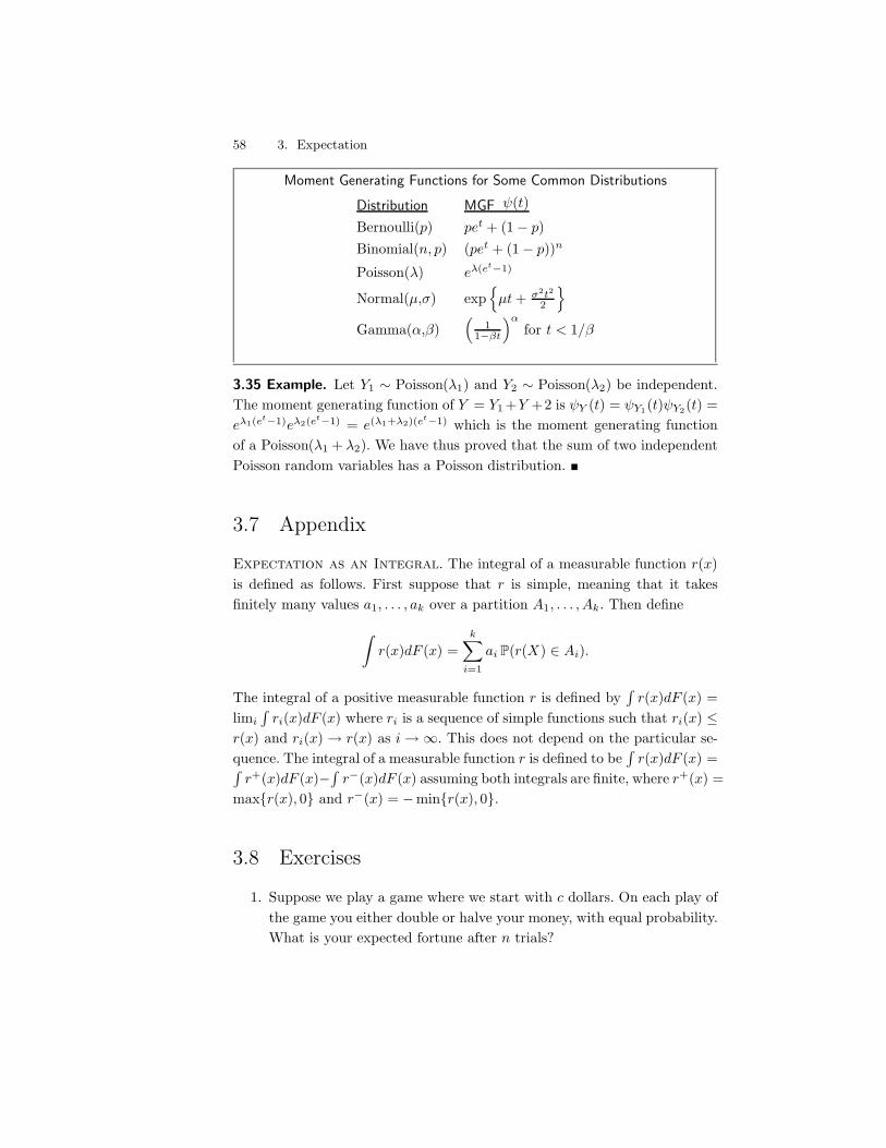
58 3. Expectation
Moment Generating Functions for Some Common Distributions
Distribution MGF ,(t)
Bernoulli(p) pet + (1" p)Binomial(n, p) (pet + (1" p))n
Poisson(%) e!(et$1)
Normal(µ,#) exp!
µt + %2t2
2
"
Gamma(),()+
11$"t
,#for t < 1/(
3.35 Example. Let Y1 ! Poisson(%1) and Y2 ! Poisson(%2) be independent.The moment generating function of Y = Y1 +Y +2 is ,Y (t) = ,Y1(t),Y2(t) =e!1(e
t$1)e!2(et$1) = e(!1+!2)(et$1) which is the moment generating function
of a Poisson(%1 + %2). We have thus proved that the sum of two independentPoisson random variables has a Poisson distribution. !
3.7 Appendix
Expectation as an Integral. The integral of a measurable function r(x)is defined as follows. First suppose that r is simple, meaning that it takesfinitely many values a1, . . . , ak over a partition A1, . . . , Ak. Then define
9r(x)dF (x) =
k*
i=1
ai P(r(X) $ Ai).
The integral of a positive measurable function r is defined by8
r(x)dF (x) =limi
8ri(x)dF (x) where ri is a sequence of simple functions such that ri(x) ,
r(x) and ri(x)) r(x) as i)#. This does not depend on the particular se-quence. The integral of a measurable function r is defined to be
8r(x)dF (x) =8
r+(x)dF (x)"8
r$(x)dF (x) assuming both integrals are finite, where r+(x) =max{r(x), 0} and r$(x) = "min{r(x), 0}.
3.8 Exercises
1. Suppose we play a game where we start with c dollars. On each play ofthe game you either double or halve your money, with equal probability.What is your expected fortune after n trials?
3.8 Exercises 59
2. Show that V(X) = 0 if and only if there is a constant c such thatP (X = c) = 1.
3. Let X1, . . . , Xn ! Uniform(0, 1) and let Yn = max{X1, . . . , Xn}. FindE(Yn).
4. A particle starts at the origin of the real line and moves along the line injumps of one unit. For each jump the probability is p that the particlewill jump one unit to the left and the probability is 1"p that the particlewill jump one unit to the right. Let Xn be the position of the particleafter n units. Find E(Xn) and V(Xn). (This is known as a randomwalk.)
5. A fair coin is tossed until a head is obtained. What is the expectednumber of tosses that will be required?
6. Prove Theorem 3.6 for discrete random variables.
7. Let X be a continuous random variable with cdf F . Suppose thatP (X > 0) = 1 and that E(X) exists. Show that E(X) =
8!0 P(X >
x)dx.
Hint: Consider integrating by parts. The following fact is helpful: if E(X)exists then limx"! x[1" F (x)] = 0.
8. Prove Theorem 3.17.
9. (Computer Experiment.) Let X1, X2, . . . , Xn be N(0, 1) random variablesand let Xn = n$1
0ni=1 Xi. Plot Xn versus n for n = 1, . . . , 10, 000.
Repeat for X1, X2, . . . , Xn ! Cauchy. Explain why there is such a dif-ference.
10. Let X ! N(0, 1) and let Y = eX . Find E(Y ) and V(Y ).
11. (Computer Experiment: Simulating the Stock Market.) Let Y1, Y2, . . . beindependent random variables such that P (Yi = 1) = P (Yi = "1) =1/2. Let Xn =
0ni=1 Yi. Think of Yi = 1 as “the stock price increased
by one dollar”, Yi = "1 as “the stock price decreased by one dollar”,and Xn as the value of the stock on day n.
(a) Find E(Xn) and V(Xn).
(b) Simulate Xn and plot Xn versus n for n = 1, 2, . . . , 10, 000. Repeatthe whole simulation several times. Notice two things. First, it’s easyto “see” patterns in the sequence even though it is random. Second,
60 3. Expectation
you will find that the four runs look very di!erent even though theywere generated the same way. How do the calculations in (a) explainthe second observation?
12. Prove the formulas given in the table at the beginning of Section 3.4for the Bernoulli, Poisson, Uniform, Exponential, Gamma, and Beta.Here are some hints. For the mean of the Poisson, use the fact thatea =
0!x=0 ax/x!. To compute the variance, first compute E(X(X"1)).
For the mean of the Gamma, it will help to multiply and divide by&() + 1)/(#+1 and use the fact that a Gamma density integrates to 1.For the Beta, multiply and divide by &()+ 1)&(()/&()+ ( + 1).
13. Suppose we generate a random variable X in the following way. Firstwe flip a fair coin. If the coin is heads, take X to have a Unif(0,1)distribution. If the coin is tails, take X to have a Unif(3,4) distribution.
(a) Find the mean of X.
(b) Find the standard deviation of X.
14. Let X1, . . . , Xm and Y1, . . . , Yn be random variables and let a1, . . . , am
and b1, . . . , bn be constants. Show that
Cov
E
Gm*
i=1
aiXi,n*
j=1
bjYj
H
J =m*
i=1
n*
j=1
aibjCov(Xi, Yj).
15. Let
fX,Y (x, y) ='
13 (x + y) 0 , x , 1, 0 , y , 20 otherwise.
Find V(2X " 3Y + 8).
16. Let r(x) be a function of x and let s(y) be a function of y. Show that
E(r(X)s(Y )|X) = r(X)E(s(Y )|X).
Also, show that E(r(X)|X) = r(X).
17. Prove thatV(Y ) = E V(Y | X) + V E(Y | X).
Hint: Let m = E(Y ) and let b(x) = E(Y |X = x). Note that E(b(X)) =EE(Y |X) = E(Y ) = m. Bear in mind that b is a function of x. Nowwrite V(Y ) = E(Y "m)2 = E((Y " b(X)) + (b(X)"m))2. Expand the
3.8 Exercises 61
square and take the expectation. You then have to take the expectationof three terms. In each case, use the rule of the iterated expectation:E(stu!) = E(E(stu!|X)).
18. Show that if E(X |Y = y) = c for some constant c, then X and Y areuncorrelated.
19. This question is to help you understand the idea of a sampling dis-tribution. Let X1, . . . , Xn be iid with mean µ and variance #2. LetXn = n$1
0ni=1 Xi. Then Xn is a statistic, that is, a function of the
data. Since Xn is a random variable, it has a distribution. This distri-bution is called the sampling distribution of the statistic. Recall fromTheorem 3.17 that E(Xn) = µ and V(Xn) = #2/n. Don’t confuse thedistribution of the data fX and the distribution of the statistic fXn
. Tomake this clear, let X1, . . . , Xn ! Uniform(0, 1). Let fX be the densityof the Uniform(0, 1). Plot fX . Now let Xn = n$1
0ni=1 Xi. Find E(Xn)
and V(Xn). Plot them as a function of n. Interpret. Now simulate thedistribution of Xn for n = 1, 5, 25, 100. Check that the simulated valuesof E(Xn) and V(Xn) agree with your theoretical calculations. What doyou notice about the sampling distribution of Xn as n increases?
20. Prove Lemma 3.21.
21. Let X and Y be random variables. Suppose that E(Y |X) = X . Showthat Cov(X, Y ) = V(X).
22. Let X ! Uniform(0, 1). Let 0 < a < b < 1. Let
Y ='
1 0 < x < b0 otherwise
and letZ =
'1 a < x < 10 otherwise
(a) Are Y and Z independent? Why/Why not?
(b) Find E(Y |Z). Hint: What values z can Z take? Now find E(Y |Z = z).
23. Find the moment generating function for the Poisson, Normal, andGamma distributions.
24. Let X1, . . . , Xn ! Exp((). Find the moment generating function of Xi.Prove that
0ni=1 Xi ! Gamma(n,().

This is page 62Printer: Opaque this
This is page 63Printer: Opaque this
4Inequalities
4.1 Probability Inequalities
Inequalities are useful for bounding quantities that might otherwise be hardto compute. They will also be used in the theory of convergence which isdiscussed in the next chapter. Our first inequality is Markov’s inequality.
4.1 Theorem (Markov’s inequality). Let X be a non-negative randomvariable and suppose that E(X) exists. For any t > 0,
P(X > t) , E(X)t
. (4.1)
Proof. Since X > 0,
E(X) =9 !
0xf(x)dx =
9 t
0xf(x)dx +
9 !
txf(x)dx
*9 !
txf(x)dx * t
9 !
tf(x)dx = t P(X > t) !

64 4. Inequalities
4.2 Theorem (Chebyshev’s inequality). Let µ = E(X) and #2 = V(X).Then,
P(|X " µ| * t) , #2
t2and P(|Z| * k) , 1
k2(4.2)
where Z = (X " µ)/#. In particular, P(|Z| > 2) , 1/4 andP(|Z| > 3) , 1/9.
Proof. We use Markov’s inequality to conclude that
P(|X " µ| * t) = P(|X " µ|2 * t2) , E(X " µ)2
t2=#2
t2.
The second part follows by setting t = k#. !
4.3 Example. Suppose we test a prediction method, a neural net for example,on a set of n new test cases. Let Xi = 1 if the predictor is wrong and Xi = 0if the predictor is right. Then Xn = n$1
0ni=1 Xi is the observed error rate.
Each Xi may be regarded as a Bernoulli with unknown mean p. We wouldlike to know the true — but unknown — error rate p. Intuitively, we expectthat Xn should be close to p. How likely is Xn to not be within - of p? Wehave that V(Xn) = V(X1)/n = p(1" p)/n and
P(|Xn " p| > -) , V(Xn)-2
=p(1" p)
n-2, 1
4n-2
since p(1" p) , 14 for all p. For - = .2 and n = 100 the bound is .0625. !
Hoe!ding’s inequality is similar in spirit to Markov’s inequality but it is asharper inequality. We present the result here in two parts.
4.4 Theorem (Hoe!ding’s Inequality). Let Y1, . . . , Yn be independentobservations such thatE(Yi) = 0 and ai , Yi , bi. Let - > 0. Then, for any t > 0,
P(
n*
i=1
Yi * -), e$t&
n/
i=1
et2(bi$ai)2/8. (4.3)
4.1 Probability Inequalities 65
4.5 Theorem. Let X1, . . . , Xn ! Bernoulli(p). Then, for any - > 0,
P;|Xn " p| > -
<, 2e$2n&2 (4.4)
where Xn = n$10n
i=1 Xi.
4.6 Example. Let X1, . . . , Xn ! Bernoulli(p). Let n = 100 and - = .2. Wesaw that Chebyshev’s inequality yielded
P(|Xn " p| > -) , .0625.
According to Hoe!ding’s inequality,
P(|Xn " p| > .2) , 2e$2(100)(.2)2 = .00067
which is much smaller than .0625. !
Hoe!ding’s inequality gives us a simple way to create a confidence inter-val for a binomial parameter p. We will discuss confidence intervals in detaillater (see Chapter 6) but here is the basic idea. Fix ) > 0 and let
-n =
T12n
log-
2)
..
By Hoe!ding’s inequality,
P;|Xn " p| > -n
<, 2e$2n&2n = ).
Let C = (Xn" -n, Xn + -n). Then, P(p /$ C) = P(|Xn" p| > -n) , ). Hence,P(p $ C) * 1 " ), that is, the random interval C traps the true parametervalue p with probability 1"); we call C a 1") confidence interval. More onthis later.
The following inequality is useful for bounding probability statements aboutNormal random variables.
4.7 Theorem (Mill’s Inequality). Let Z ! N(0, 1). Then,
P(|Z| > t) ,U
2&
e$t2/2
t.
66 4. Inequalities
4.2 Inequalities For Expectations
This section contains two inequalities on expected values.
4.8 Theorem (Cauchy-Schwartz inequality). If X and Y have finitevariances then
E |XY | ,3
E(X2)E(Y 2). (4.5)
Recall that a function g is convex if for each x, y and each ) $ [0, 1],
g()x + (1" ))y) , )g(x) + (1 " ))g(y).
If g is twice di!erentiable and g&&(x) * 0 for all x, then g is convex. It canbe shown that if g is convex, then g lies above any line that touches g atsome point, called a tangent line. A function g is concave if "g is convex.Examples of convex functions are g(x) = x2 and g(x) = ex. Examples ofconcave functions are g(x) = "x2 and g(x) = log x.
4.9 Theorem (Jensen’s inequality). If g is convex, then
Eg(X) * g(EX). (4.6)
If g is concave, thenEg(X) , g(EX). (4.7)
Proof. Let L(x) = a + bx be a line, tangent to g(x) at the point E(X).Since g is convex, it lies above the line L(x). So,
Eg(X) * EL(X) = E(a + bX) = a + bE(X) = L(E(X)) = g(EX). !
From Jensen’s inequality we see that E(X2) * (EX)2 and if X is positive,then E(1/X) * 1/E(X). Since log is concave, E(log X) , log E(X).
4.3 Bibliographic Remarks
Devroye et al. (1996) is a good reference on probability inequalities and theiruse in statistics and pattern recognition. The following proof of Hoe!ding’sinequality is from that text.
4.4 Appendix 67
4.4 Appendix
Proof of Hoeffding’s Inequality. We will make use of the exact form ofTaylor’s theorem: if g is a smooth function, then there is a number . $ (0, u)such that g(u) = g(0) + ug&(0) + u2
2 g""(.).
Proof of Theorem 4.4. For any t > 0, we have, from Markov’s inequality,that
P(
n*
i=1
Yi * -)
= P(
tn*
i=1
Yi * t-
)= P
+et0n
i=1 Yi * et&,
, e$t&E+et0n
i=1 Yi
,= e$t&
/
i
E(etYi). (4.8)
Since ai , Yi , bi, we can write Yi as a convex combination of ai and bi,namely, Yi = )bi + (1 " ))ai where ) = (Yi " ai)/(bi " ai). So, by theconvexity of ety we have
etYi , Yi " ai
bi " aietbi +
bi " Yi
bi " aietai .
Take expectations of both sides and use the fact that E(Yi) = 0 to get
EetYi , " ai
bi " aietbi +
bi
bi " aietai = eg(u) (4.9)
where u = t(bi " ai), g(u) = "/u + log(1" / + /eu) and / = "ai/(bi " ai).Note that g(0) = g&(0) = 0. Also, g
""(u) , 1/4 for all u > 0. By Taylor’s
theorem, there is a . $ (0, u) such that
g(u) = g(0) + ug"(0) +
u2
2g
""(.)
=u2
2g
""(.) , u2
8=
t2(bi " ai)2
8.
Hence,EetYi , eg(u) , et2(bi$ai)
2/8.
The result follows from (4.8). !
Proof of Theorem 4.5. Let Yi = (1/n)(Xi " p). Then E(Yi) = 0 anda , Yi , b where a = "p/n and b = (1 " p)/n. Also, (b " a)2 = 1/n2.Applying Theorem 4.4 we get
P(Xn " p > -) = P(*
i
Yi > -
), e$t&et2/(8n).
The above holds for any t > 0. In particular, take t = 4n- and we get P(Xn"p > -) , e$2n&2 . By a similar argument we can show that P(Xn " p < "-) ,e$2n&2. Putting these together we get P
;|Xn " p| > -
<, 2e$2n&2 . !
68 4. Inequalities
4.5 Exercises
1. Let X ! Exponential((). Find P(|X " µX | * k#X) for k > 1. Comparethis to the bound you get from Chebyshev’s inequality.
2. Let X ! Poisson(%). Use Chebyshev’s inequality to show that P(X *2%) , 1/%.
3. Let X1, . . . , Xn ! Bernoulli(p) and Xn = n$10n
i=1 Xi. Bound P(|Xn"p| > -) using Chebyshev’s inequality and using Hoe!ding’s inequality.Show that, when n is large, the bound from Hoe!ding’s inequality issmaller than the bound from Chebyshev’s inequality.
4. Let X1, . . . , Xn ! Bernoulli(p).
(a) Let ) > 0 be fixed and define
-n =
T12n
log-
2)
..
Let 1pn = n$10n
i=1 Xi. Define Cn = (1pn " -n, 1pn + -n). Use Hoe!ding’sinequality to show that
P(Cn contains p) * 1" ).
In practice, we truncate the interval so it does not go below 0 or above1.
(b) (Computer Experiment.) Let’s examine the properties of this confi-dence interval. Let ) = 0.05 and p = 0.4. Conduct a simulation studyto see how often the interval contains p (called the coverage). Do thisfor various values of n between 1 and 10000. Plot the coverage versus n.
(c) Plot the length of the interval versus n. Suppose we want the lengthof the interval to be no more than .05. How large should n be?
5. Prove Mill’s inequality, Theorem 4.7. Hint. Note that P(|Z| > t) =2P(Z > t). Now write out what P(Z > t) means and note that x/t > 1whenever x > t.
6. Let Z ! N(0, 1). Find P(|Z| > t) and plot this as a function of t. FromMarkov’s inequality, we have the bound P(|Z| > t) , E|Z|k
tk for anyk > 0. Plot these bounds for k = 1, 2, 3, 4, 5 and compare them to thetrue value of P(|Z| > t). Also, plot the bound from Mill’s inequality.
4.5 Exercises 69
7. Let X1, . . . , Xn ! N(0, 1). Bound P(|Xn| > t) using Mill’s inequality,where Xn = n$1
0ni=1 Xi. Compare to the Chebyshev bound.

This is page 70Printer: Opaque this
This is page 71Printer: Opaque this
5Convergence of Random Variables
5.1 Introduction
The most important aspect of probability theory concerns the behavior ofsequences of random variables. This part of probability is called large sampletheory, or limit theory, or asymptotic theory. The basic question is this:what can we say about the limiting behavior of a sequence of random variablesX1, X2, X3, . . .? Since statistics and data mining are all about gathering data,we will naturally be interested in what happens as we gather more and moredata.
In calculus we say that a sequence of real numbers xn converges to a limitx if, for every - > 0, |xn"x| < - for all large n. In probability, convergence ismore subtle. Going back to calculus for a moment, suppose that xn = x forall n. Then, trivially, limn"! xn = x. Consider a probabilistic version of thisexample. Suppose that X1, X2, . . . is a sequence of random variables whichare independent and suppose each has a N(0, 1) distribution. Since these allhave the same distribution, we are tempted to say that Xn “converges” toX ! N(0, 1). But this can’t quite be right since P(Xn = X) = 0 for all n.(Two continuous random variables are equal with probability zero.)
Here is another example. Consider X1, X2, . . . where Xi ! N(0, 1/n). Intu-itively, Xn is very concentrated around 0 for large n so we would like to saythat Xn converges to 0. But P(Xn = 0) = 0 for all n. Clearly, we need to
72 5. Convergence of Random Variables
develop some tools for discussing convergence in a rigorous way. This chapterdevelops the appropriate methods.
There are two main ideas in this chapter which we state informally here:
1. The law of large numbers says that the sample average Xn = n$10n
i=1 Xi
converges in probability to the expectation µ = E(Xi). This meansthat Xn is close to µ with high probability.
2. The central limit theorem says that/
n(Xn"µ) converges in dis-tribution to a Normal distribution. This means that the sample averagehas approximately a Normal distribution for large n.
5.2 Types of Convergence
The two main types of convergence are defined as follows.
5.1 Definition. Let X1, X2, . . . be a sequence of random variables and letX be another random variable. Let Fn denote the cdf of Xn and let F
denote the cdf of X.
1. Xn converges to X in probability, written XnP")X, if, for every
- > 0,P(|Xn "X | > -)) 0 (5.1)
as n)#.
2. Xn converges to X in distribution, written Xn ! X, if
limn"!
Fn(t) = F (t) (5.2)
at all t for which F is continuous.
When the limiting random variable is a point mass, we change the notationslightly. If P(X = c) = 1 and Xn
P")X then we write XnP") c. Similarly, if
Xn ! X we write Xn ! c.There is another type of convergence which we introduce mainly because it
is useful for proving convergence in probability.
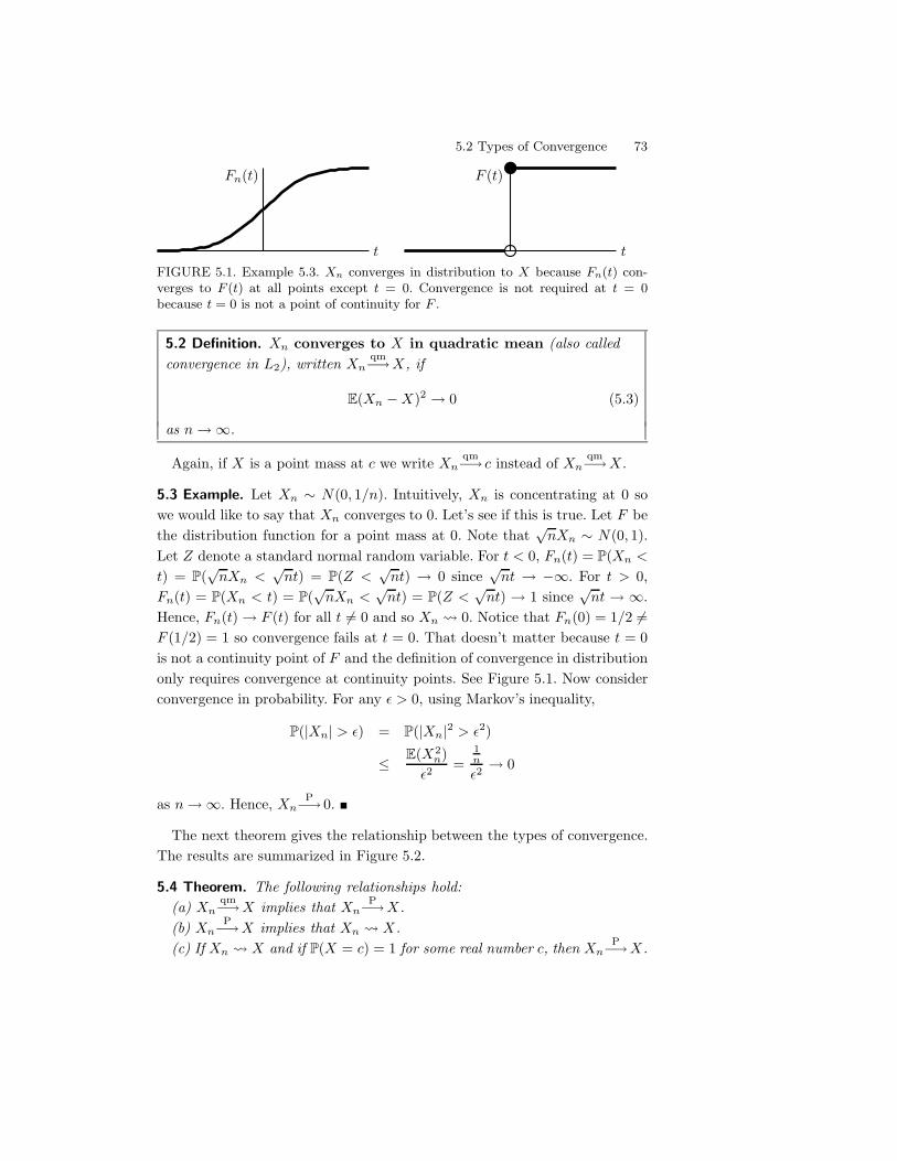
5.2 Types of Convergence 73
t
Fn(t)
t
F (t)
FIGURE 5.1. Example 5.3. Xn converges in distribution to X because Fn(t) con-verges to F (t) at all points except t = 0. Convergence is not required at t = 0because t = 0 is not a point of continuity for F .
5.2 Definition. Xn converges to X in quadratic mean (also calledconvergence in L2), written Xn
qm")X, if
E(Xn "X)2 ) 0 (5.3)
as n)#.
Again, if X is a point mass at c we write Xnqm") c instead of Xn
qm")X .
5.3 Example. Let Xn ! N(0, 1/n). Intuitively, Xn is concentrating at 0 sowe would like to say that Xn converges to 0. Let’s see if this is true. Let F bethe distribution function for a point mass at 0. Note that
/nXn ! N(0, 1).
Let Z denote a standard normal random variable. For t < 0, Fn(t) = P(Xn <
t) = P(/
nXn </
nt) = P(Z </
nt) ) 0 since/
nt ) "#. For t > 0,Fn(t) = P(Xn < t) = P(
/nXn <
/nt) = P(Z <
/nt) ) 1 since
/nt ) #.
Hence, Fn(t)) F (t) for all t (= 0 and so Xn ! 0. Notice that Fn(0) = 1/2 (=F (1/2) = 1 so convergence fails at t = 0. That doesn’t matter because t = 0is not a continuity point of F and the definition of convergence in distributiononly requires convergence at continuity points. See Figure 5.1. Now considerconvergence in probability. For any - > 0, using Markov’s inequality,
P(|Xn| > -) = P(|Xn|2 > -2)
, E(X2n)
-2=
1n
-2) 0
as n)#. Hence, XnP") 0. !
The next theorem gives the relationship between the types of convergence.The results are summarized in Figure 5.2.
5.4 Theorem. The following relationships hold:(a) Xn
qm")X implies that XnP")X.
(b) XnP")X implies that Xn ! X.
(c) If Xn ! X and if P(X = c) = 1 for some real number c, then XnP")X.
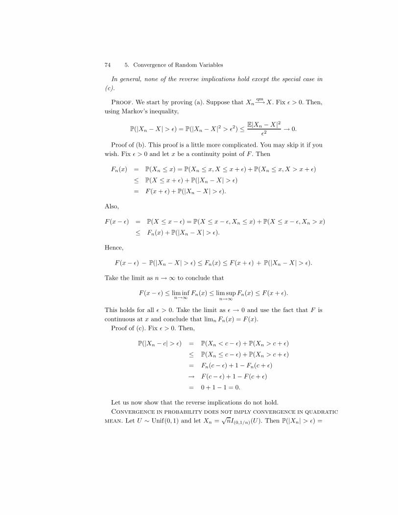
74 5. Convergence of Random Variables
In general, none of the reverse implications hold except the special case in(c).
Proof. We start by proving (a). Suppose that Xnqm")X . Fix - > 0. Then,
using Markov’s inequality,
P(|Xn "X | > -) = P(|Xn "X |2 > -2) , E|Xn "X |2-2
) 0.
Proof of (b). This proof is a little more complicated. You may skip it if youwish. Fix - > 0 and let x be a continuity point of F . Then
Fn(x) = P(Xn , x) = P(Xn , x, X , x + -) + P(Xn , x, X > x + -)
, P(X , x + -) + P(|Xn "X | > -)
= F (x + -) + P(|Xn "X | > -).
Also,
F (x" -) = P(X , x" -) = P(X , x" -, Xn , x) + P(X , x" -, Xn > x)
, Fn(x) + P(|Xn "X | > -).
Hence,
F (x" -) " P(|Xn "X | > -) , Fn(x) , F (x + -) + P(|Xn "X | > -).
Take the limit as n)# to conclude that
F (x" -) , lim infn"!
Fn(x) , lim supn"!
Fn(x) , F (x + -).
This holds for all - > 0. Take the limit as - ) 0 and use the fact that F iscontinuous at x and conclude that limn Fn(x) = F (x).
Proof of (c). Fix - > 0. Then,
P(|Xn " c| > -) = P(Xn < c" -) + P(Xn > c + -)
, P(Xn , c" -) + P(Xn > c + -)
= Fn(c" -) + 1" Fn(c + -)
) F (c" -) + 1" F (c + -)
= 0 + 1" 1 = 0.
Let us now show that the reverse implications do not hold.Convergence in probability does not imply convergence in quadratic
mean. Let U ! Unif(0, 1) and let Xn =/
nI(0,1/n)(U). Then P(|Xn| > -) =
5.2 Types of Convergence 75
quadratic mean probability distribution
point-mass distribution
FIGURE 5.2. Relationship between types of convergence.
P(/
nI(0,1/n)(U) > -) = P(0 , U < 1/n) = 1/n ) 0. Hence, XnP") 0. But
E(X2n) = n
8 1/n0 du = 1 for all n so Xn does not converge in quadratic mean.
Convergence in distribution does not imply convergence in prob-
ability. Let X ! N(0, 1). Let Xn = "X for n = 1, 2, 3, . . .; hence Xn !N(0, 1). Xn has the same distribution function as X for all n so, trivially,limn Fn(x) = F (x) for all x. Therefore, Xn ! X . But P(|Xn " X | > -) =P(|2X | > -) = P(|X | > -/2) (= 0. So Xn does not converge to X in probability.!
Warning! One might conjecture that if XnP") b, then E(Xn)) b. This is
not1 true. Let Xn be a random variable defined by P(Xn = n2) = 1/n andP(Xn = 0) = 1 " (1/n). Now, P(|Xn| < -) = P(Xn = 0) = 1 " (1/n) ) 1.Hence, Xn
P") 0. However, E(Xn) = [n2- (1/n)]+ [0- (1" (1/n))] = n. Thus,E(Xn))#.
Summary. Stare at Figure 5.2.Some convergence properties are preserved under transformations.
5.5 Theorem. Let Xn, X, Yn, Y be random variables. Let g be a continuousfunction.
(a) If XnP")X and Yn
P")Y , then Xn + YnP")X + Y .
(b) If Xnqm")X and Yn
qm")Y , then Xn + Ynqm")X + Y .
(c) If Xn ! X and Yn ! c, then Xn + Yn ! X + c.(d) If Xn
P")X and YnP")Y , then XnYn
P")XY .(e) If Xn ! X and Yn ! c, then XnYn ! cX.(f) If Xn
P")X, then g(Xn) P") g(X).(g) If Xn ! X, then g(Xn) ! g(X).
Parts (c) and (e) are know as Slutzky’s theorem. It is worth noting thatXn ! X and Yn ! Y does not in general imply that Xn + Yn ! X + Y .
1We can conclude that E(Xn) $ b if Xn is uniformly integrable. See the appendix.
76 5. Convergence of Random Variables
5.3 The Law of Large Numbers
Now we come to a crowning achievement in probability, the law of large num-bers. This theorem says that the mean of a large sample is close to the meanof the distribution. For example, the proportion of heads of a large numberof tosses is expected to be close to 1/2. We now make this more precise.
Let X1, X2, . . . be an iid sample, let µ = E(X1) and 2 #2 = V(X1). Recallthat the sample mean is defined as Xn = n$1
0ni=1 Xi and that E(Xn) = µ
and V(Xn) = #2/n.
5.6 Theorem (The Weak Law of Large Numbers (WLLN)). 3
If X1, . . . , Xn are iid, then XnP")µ.
Interpretation of the WLLN: The distribution of Xn becomes more
concentrated around µ as n gets large.
Proof. Assume that # < #. This is not necessary but it simplifies theproof. Using Chebyshev’s inequality,
P;|Xn " µ| > -
<, V(Xn)
-2=
#2
n-2
which tends to 0 as n)#. !
5.7 Example. Consider flipping a coin for which the probability of heads isp. Let Xi denote the outcome of a single toss (0 or 1). Hence, p = P (Xi =1) = E(Xi). The fraction of heads after n tosses is Xn. According to the lawof large numbers, Xn converges to p in probability. This does not mean thatXn will numerically equal p. It means that, when n is large, the distributionof Xn is tightly concentrated around p. Suppose that p = 1/2. How largeshould n be so that P (.4 , Xn , .6) * .7? First, E(Xn) = p = 1/2 andV(Xn) = #2/n = p(1" p)/n = 1/(4n). From Chebyshev’s inequality,
P(.4 , Xn , .6) = P(|Xn " µ| , .1)
= 1" P(|Xn " µ| > .1)
* 1" 14n(.1)2
= 1" 25n
.
The last expression will be larger than .7 if n = 84. !
2Note that µ = E(Xi) is the same for all i so we can define µ = E(Xi) for any i. Byconvention, we often write µ = E(X1).
3There is a stronger theorem in the appendix called the strong law of large numbers.
5.4 The Central Limit Theorem 77
5.4 The Central Limit Theorem
The law of large numbers says that the distribution of Xn piles up near µ.This isn’t enough to help us approximate probability statements about Xn.For this we need the central limit theorem.
Suppose that X1, . . . , Xn are iid with mean µ and variance #2. The centrallimit theorem (CLT) says that Xn = n$1
0i Xi has a distribution which is
approximately Normal with mean µ and variance #2/n. This is remarkablesince nothing is assumed about the distribution of Xi, except the existence ofthe mean and variance.
5.8 Theorem (The Central Limit Theorem (CLT)). Let X1, . . . , Xn be iid
with mean µ and variance #2. Let Xn = n$10n
i=1 Xi. Then
Zn 0Xn " µV
V(Xn)=/
n(Xn " µ)#
! Z
where Z ! N(0, 1). In other words,
limn"!
P(Zn , z) = %(z) =9 z
$!
1/2&
e$x2/2dx.
Interpretation: Probability statements about Xn can be approximated
using a Normal distribution. It’s the probability statements that we
are approximating, not the random variable itself.
In addition to Zn ! N(0, 1), there are several forms of notation to denotethe fact that the distribution of Zn is converging to a Normal. They all meanthe same thing. Here they are:
Zn . N(0, 1)
Xn . N
-µ,
#2
n
.
Xn " µ . N
-0,#2
n
.
/n(Xn " µ) . N
;0, #2
<
/n(Xn " µ)
#. N(0, 1).
5.9 Example. Suppose that the number of errors per computer program has aPoisson distribution with mean 5. We get 125 programs. Let X1, . . . , X125 be
78 5. Convergence of Random Variables
the number of errors in the programs. We want to approximate P(Xn < 5.5).Let µ = E(X1) = % = 5 and #2 = V(X1) = % = 5. Then,
P(Xn < 5.5) = P-/
n(Xn " µ)#
<
/n(5.5" µ)
#
.
. P(Z < 2.5) = .9938. !
The central limit theorem tells us that Zn =/
n(Xn"µ)/# is approximatelyN(0,1). However, we rarely know #. Later, we will see that we can estimate#2 from X1, . . . , Xn by
S2n =
1n" 1
n*
i=1
(Xi "Xn)2.
This raises the following question: if we replace # with Sn, is the central limittheorem still true? The answer is yes.
5.10 Theorem. Assume the same conditions as the CLT. Then,/
n(Xn " µ)Sn
! N(0, 1).
You might wonder, how accurate the normal approximation is. The answeris given in the Berry-Esseen theorem.
5.11 Theorem (The Berry-Esseen Inequality). Suppose that E|X1|3 <#. Then
supz
|P(Zn , z)" %(z)| , 334
E|X1 " µ|3/n#3
. (5.4)
There is also a multivariate version of the central limit theorem.
5.12 Theorem (Multivariate central limit theorem). Let X1, . . . , Xn be iid ran-dom vectors where
Xi =
E
FFFG
X1i
X2i...
Xki
H
IIIJ
with mean
µ =
E
FFFG
µ1
µ2...
µk
H
IIIJ=
E
FFFG
E(X1i)E(X2i)
...E(Xki)
H
IIIJ
5.5 The Delta Method 79
and variance matrix '. Let
X =
E
FFFG
X1
X2...
Xk
H
IIIJ.
where Xj = n$10n
i=1 Xji. Then,/
n(X " µ) ! N(0,').
5.5 The Delta Method
If Yn has a limiting Normal distribution then the delta method allows us tofind the limiting distribution of g(Yn) where g is any smooth function.
5.13 Theorem (The Delta Method). Suppose that/
n(Yn " µ)#
! N(0, 1)
and that g is a di!erentiable function such that g&(µ) (= 0. Then/
n(g(Yn)" g(µ))|g&(µ)|# ! N(0, 1).
In other words,
Yn . N
(µ,#2
n
)implies that g(Yn) . N
(g(µ), (g&(µ))2
#2
n
).
5.14 Example. Let X1, . . . , Xn be iid with finite mean µ and finite variance#2. By the central limit theorem,
/n(Xn " µ)/# ! N(0, 1). Let Wn = eXn .
Thus, Wn = g(Xn) where g(s) = es. Since g&(s) = es, the delta methodimplies that Wn . N(eµ, e2µ#2/n). !
There is also a multivariate version of the delta method.
5.15 Theorem (The Multivariate Delta Method). Suppose that Yn = (Yn1, . . . , Ynk)is a sequence of random vectors such that
/n(Yn " µ) ! N(0,').
80 5. Convergence of Random Variables
Let g : Rk ) R and let
1g(y) =
E
FFG
'g'y1...'g'yk
H
IIJ .
Let 1µ denote 1g(y) evaluated at y = µ and assume that the elements of 1µ
are nonzero. Then/
n(g(Yn)" g(µ)) ! N;0,1T
µ'1µ
<.
5.16 Example. Let-
X11
X21
.,
-X12
X22
., . . . ,
-X1n
X2n
.
be iid random vectors with mean µ = (µ1, µ2)T and variance '. Let
X1 =1n
n*
i=1
X1i, X2 =1n
n*
i=1
X2i
and define Yn = X1X2. Thus, Yn = g(X1, X2) where g(s1, s2) = s1s2. By thecentral limit theorem,
/n
-X1 " µ1
X2 " µ2
.! N(0,').
Now
1g(s) =
('g's1'g's2
)=-
s2
s1
.
and so
1Tµ'1µ = (µ2 µ1)
-#11 #12
#12 #22
.-µ2
µ1
.= µ2
2#11 + 2µ1µ2#12 + µ21#22.
Therefore,
/n(X1X2 " µ1µ2) ! N
-0, µ2
2#11 + 2µ1µ2#12 + µ21#22
.. !
5.6 Bibliographic Remarks
Convergence plays a central role in modern probability theory. For more de-tails, see Grimmett and Stirzaker (1982), Karr (1993), and Billingsley (1979).Advanced convergence theory is explained in great detail in van der Vaartand Wellner (1996) and and van der Vaart (1998).
5.7 Appendix 81
5.7 Appendix
5.7.1 Almost Sure and L1 Convergence
We say that Xn converges almost surely to X , written Xnas")X , if
P({s : Xn(s)) X(s)}) = 1.
We say that Xn converges in L1 to X , written XnL1")X , if
E|Xn "X |) 0
as n)#.
5.17 Theorem. Let Xn and X be random variables. Then:(a) Xn
as")X implies that XnP")X.
(b) Xnqm")X implies that Xn
L1")X.(c) Xn
L1")X implies that XnP")X.
The weak law of large numbers says that Xn converges to E(X1) in proba-bility. The strong law asserts that this is also true almost surely.
5.18 Theorem (The Strong Law of Large Numbers). Let X1, X2, . . . be iid. Ifµ = E|X1| <# then Xn
as")µ.
A sequence Xn is asymptotically uniformly integrable if
limM"!
lim supn"!
E (|Xn|I(|Xn| > M)) = 0.
5.19 Theorem. If XnP") b and Xn is asymptotically uniformly integrable,
then E(Xn)) b.
5.7.2 Proof of the Central Limit Theorem
Recall that if X is a random variable, its moment generating function (mgf)is ,X(t) = EetX . Assume in what follows that the mgf is finite in a neigh-borhood around t = 0.
5.20 Lemma. Let Z1, Z2, . . . be a sequence of random variables. Let ,n be themgf of Zn. Let Z be another random variable and denote its mgf by ,. If,n(t)) ,(t) for all t in some open interval around 0, then Zn ! Z.
82 5. Convergence of Random Variables
proof of the central limit theorem. Let Yi = (Xi " µ)/#. Then,Zn = n$1/2
0i Yi. Let ,(t) be the mgf of Yi. The mgf of
0i Yi is (,(t))n
and mgf of Zn is [,(t//
n)]n 0 .n(t). Now ,&(0) = E(Y1) = 0, ,&&(0) =E(Y 2
1 ) = V(Y1) = 1. So,
,(t) = ,(0) + t,&(0) +t2
2!,&&(0) +
t3
3!,&&&(0) + · · ·
= 1 + 0 +t2
2+
t3
3!,&&&(0) + · · ·
= 1 +t2
2+
t3
3!,&&&(0) + · · ·
Now,
.n(t) =A,
-t/n
.Bn
=A1 +
t2
2n+
t3
3!n3/2,&&&(0) + · · ·
Bn
=
W1 +
t2
2 + t3
3!n1/2,&&&(0) + · · ·
n
Xn
) et2/2
which is the mgf of a N(0,1). The result follows from the previous Theorem.In the last step we used the fact that if an ) a then
+1 +
an
n
,n) ea. !
5.8 Exercises
1. Let X1, . . . , Xn be iid with finite mean µ = E(X1) and finite variance#2 = V(X1). Let Xn be the sample mean and let S2
n be the samplevariance.
(a) Show that E(S2n) = #2.
(b) Show that S2n
P")#2. Hint: Show that S2n = cnn$1
0ni=1 X2
i " dnX2n
where cn ) 1 and dn ) 1. Apply the law of large numbers to n$10n
i=1 X2i
and to Xn. Then use part (e) of Theorem 5.5.
2. Let X1, X2, . . . be a sequence of random variables. Show that Xnqm") b
if and only if
limn"!
E(Xn) = b and limn"!
V(Xn) = 0.
5.8 Exercises 83
3. Let X1, . . . , Xn be iid and let µ = E(X1). Suppose that the variance isfinite. Show that Xn
qm")µ.
4. Let X1, X2, . . . be a sequence of random variables such that
P-
Xn =1n
.= 1" 1
n2and P (Xn = n) =
1n2
.
Does Xn converge in probability? Does Xn converge in quadratic mean?
5. Let X1, . . . , Xn ! Bernoulli(p). Prove that
1n
n*
i=1
X2i
P") p and1n
n*
i=1
X2i
qm") p.
6. Suppose that the height of men has mean 68 inches and standard de-viation 2.6 inches. We draw 100 men at random. Find (approximately)the probability that the average height of men in our sample will be atleast 68 inches.
7. Let %n = 1/n for n = 1, 2, . . .. Let Xn ! Poisson(%n).
(a) Show that XnP") 0.
(b) Let Yn = nXn. Show that YnP") 0.
8. Suppose we have a computer program consisting of n = 100 pages ofcode. Let Xi be the number of errors on the ith page of code. Supposethat the X &
is are Poisson with mean 1 and that they are independent.Let Y =
0ni=1 Xi be the total number of errors. Use the central limit
theorem to approximate P(Y < 90).
9. Suppose that P(X = 1) = P(X = "1) = 1/2. Define
Xn ='
X with probability 1" 1n
en with probability 1n .
Does Xn converge to X in probability? Does Xn converge to X in dis-tribution? Does E(X "Xn)2 converge to 0?
10. Let Z ! N(0, 1). Let t > 0. Show that, for any k > 0,
P(|Z| > t) , E|Z|k
tk.
Compare this to Mill’s inequality in Chapter 4.
84 5. Convergence of Random Variables
11. Suppose that Xn ! N(0, 1/n) and let X be a random variable withdistribution F (x) = 0 if x < 0 and F (x) = 1 if x * 0. Does Xn convergeto X in probability? (Prove or disprove). Does Xn converge to X indistribution? (Prove or disprove).
12. Let X, X1, X2, X3, . . . be random variables that are positive and integervalued. Show that Xn ! X if and only if
limn"!
P(Xn = k) = P(X = k)
for every integer k.
13. Let Z1, Z2, . . . be iid random variables with density f . Suppose thatP(Zi > 0) = 1 and that % = limx)0 f(x) > 0. Let
Xn = n min{Z1, . . . , Zn}.
Show that Xn ! Z where Z has an exponential distribution with mean1/%.
14. Let X1, . . . , Xn ! Uniform(0, 1). Let Yn = X2n. Find the limiting distri-
bution of Yn.
15. Let -X11
X21
.,
-X12
X22
., . . . ,
-X1n
X2n
.
be iid random vectors with mean µ = (µ1, µ2) and variance '. Let
X1 =1n
n*
i=1
X1i, X2 =1n
n*
i=1
X2i
and define Yn = X1/X2. Find the limiting distribution of Yn.
16. Construct an example where Xn ! X and Yn ! Y but Xn + Yn doesnot converge in distribution to X + Y .
Part II
Statistical Inference

This is pagePrinter: Opaque this
This is page 87Printer: Opaque this
6Models, Statistical Inference andLearning
6.1 Introduction
Statistical inference, or “learning” as it is called in computer science, is theprocess of using data to infer the distribution that generated the data. Atypical statistical inference question is:
Given a sample X1, . . . , Xn ! F , how do we infer F?
In some cases, we may want to infer only some feature of F such as itsmean.
6.2 Parametric and Nonparametric Models
A statistical model F is a set of distributions (or densities or regressionfunctions). A parametric model is a set F that can be parameterized by afinite number of parameters. For example, if we assume that the data comefrom a Normal distribution, then the model is
F ='
f(x; µ,#) =1
#/
2&exp'" 1
2#2(x" µ)2
2, µ $ R, # > 0
2. (6.1)
This is a two-parameter model. We have written the density as f(x; µ,#) toshow that x is a value of the random variable whereas µ and # are parameters.
88 6. Models, Statistical Inference and Learning
In general, a parametric model takes the form
F =
:f(x; 0) : 0 $ "
Y(6.2)
where 0 is an unknown parameter (or vector of parameters) that can takevalues in the parameter space ". If 0 is a vector but we are only interested inone component of 0, we call the remaining parameters nuisance parameters.A nonparametric model is a set F that cannot be parameterized by a finitenumber of parameters. For example, FALL = {all cdf&s} is nonparametric. 1
6.1 Example (One-dimensional Parametric Estimation). Let X1, . . ., Xn be in-dependent Bernoulli(p) observations. The problem is to estimate the param-eter p. !
6.2 Example (Two-dimensional Parametric Estimation). Suppose that X1, . . .,Xn ! F and we assume that the pdf f $ F where F is given in (6.1). Inthis case there are two parameters, µ and #. The goal is to estimate theparameters from the data. If we are only interested in estimating µ, then µ isthe parameter of interest and # is a nuisance parameter. !
6.3 Example (Nonparametric estimation of the cdf). Let X1, . . ., Xn be inde-pendent observations from a cdf F . The problem is to estimate F assumingonly that F $ FALL = {all cdf&s}. !
6.4 Example (Nonparametric density estimation). Let X1, . . . , Xn be indepen-dent observations from a cdf F and let f = F & be the pdf. Suppose we wantto estimate the pdf f . It is not possible to estimate f assuming only thatF $ FALL. We need to assume some smoothness on f . For example, we mightassume that f $ F = FDENS
%FSOB where FDENS is the set of all probability
density functions and
FSOB ='
f :9
(f &&(x))2dx <#2
.
The class FSOB is called a Sobolev space; it is the set of functions that arenot “too wiggly.” !
6.5 Example (Nonparametric estimation of functionals). Let X1, . . ., Xn ! F .Suppose we want to estimate µ = E(X1) =
8xdF (x) assuming only that
1The distinction between parametric and nonparametric is more subtle than this but we don’tneed a rigorous definition for our purposes.
6.2 Parametric and Nonparametric Models 89
µ exists. The mean µ may be thought of as a function of F : we can writeµ = T (F ) =
8xdF (x). In general, any function of F is called a statis-
tical functional. Other examples of functionals are the variance T (F ) =8x2dF (x) "
;8xdF (x)
<2 and the median T (F ) = F$1(1/2). !
6.6 Example (Regression, prediction, and classification). Suppose we observe pairsof data (X1, Y1), . . . (Xn, Yn). Perhaps Xi is the blood pressure of subject i
and Yi is how long they live. X is called a predictor or regressor or fea-ture or independent variable. Y is called the outcome or the responsevariable or the dependent variable. We call r(x) = E(Y |X = x) the re-gression function. If we assume that r $ F where F is finite dimensional —the set of straight lines for example — then we have a parametric regres-sion model. If we assume that r $ F where F is not finite dimensional thenwe have a nonparametric regression model. The goal of predicting Y fora new patient based on their X value is called prediction. If Y is discrete(for example, live or die) then prediction is instead called classification. Ifour goal is to estimate the function r, then we call this regression or curveestimation. Regression models are sometimes written as
Y = r(X) + - (6.3)
where E(-) = 0. We can always rewrite a regression model this way. To seethis, define - = Y " r(X) and hence Y = Y + r(X) " r(X) = r(X) + -.Moreover, E(-) = EE(-|X) = E(E(Y " r(X))|X) = E(E(Y |X) " r(X)) =E(r(X)" r(X)) = 0. !
What’s Next? It is traditional in most introductory courses to start withparametric inference. Instead, we will start with nonparametric inference andthen we will cover parametric inference. In some respects, nonparametric in-ference is easier to understand and is more useful than parametric inference.
Frequentists and Bayesians. There are many approaches to statisticalinference. The two dominant approaches are called frequentist inferenceand Bayesian inference. We’ll cover both but we will start with frequentistinference. We’ll postpone a discussion of the pros and cons of these two untillater.
Some Notation. If F = {f(x; 0) : 0 $ "} is a parametric model, we writeP((X $ A) =
8A f(x; 0)dx and E((r(X)) =
8r(x)f(x; 0)dx. The subscript 0
indicates that the probability or expectation is with respect to f(x; 0); it doesnot mean we are averaging over 0. Similarly, we write V( for the variance.
90 6. Models, Statistical Inference and Learning
6.3 Fundamental Concepts in Inference
Many inferential problems can be identified as being one of three types: es-timation, confidence sets, or hypothesis testing. We will treat all of theseproblems in detail in the rest of the book. Here, we give a brief introductionto the ideas.
6.3.1 Point Estimation
Point estimation refers to providing a single “best guess” of some quantityof interest. The quantity of interest could be a parameter in a parametricmodel, a cdf F , a probability density function f , a regression function r, ora prediction for a future value Y of some random variable.
By convention, we denote a point estimate of 0 by 10 or 10n. Remember
that 0 is a fixed, unknown quantity. The estimate 10 depends on the
data so 10 is a random variable.
More formally, let X1, . . . , Xn be n iid data points from some distributionF . A point estimator 10n of a parameter 0 is some function of X1, . . . , Xn:
10n = g(X1, . . . , Xn).
The bias of an estimator is defined by
bias(10n) = E((10n)" 0. (6.4)
We say that 10n is unbiased if E(10n) = 0. Unbiasedness used to receive muchattention but these days is considered less important; many of the estimatorswe will use are biased. A reasonable requirement for an estimator is that itshould converge to the true parameter value as we collect more and moredata. This requirement is quantified by the following definition:
6.7 Definition. A point estimator 10n of a parameter 0 is consistent if10n
P") 0.
The distribution of 10n is called the sampling distribution. The standarddeviation of 10n is called the standard error, denoted by se:
se = se(10n) =V
V(10n). (6.5)
Often, the standard error depends on the unknown F . In those cases, se isan unknown quantity but we usually can estimate it. The estimated standarderror is denoted by 1se.
6.3 Fundamental Concepts in Inference 91
6.8 Example. Let X1, . . . , Xn ! Bernoulli(p) and let 1pn = n$10
i Xi. ThenE(1pn) = n$1
0i E(Xi) = p so 1pn is unbiased. The standard error is se =3
V(1pn) =3
p(1" p)/n. The estimated standard error is 1se =31p(1" 1p)/n.
!
The quality of a point estimate is sometimes assessed by the mean squarederror, or mse defined by
mse = E((10n " 0)2. (6.6)
Keep in mind that E((·) refers to expectation with respect to the distribution
f(x1, . . . , xn; 0) =n/
i=1
f(xi; 0)
that generated the data. It does not mean we are averaging over a distributionfor 0.
6.9 Theorem. The mse can be written as
mse = bias2(10n) + V((10n). (6.7)
Proof. Let 0n = E((10n). Then
E((10n " 0)2 = E((10n " 0n + 0n " 0)2
= E((10n " 0n)2 + 2(0n " 0)E((10n " 0n) + E((0n " 0)2
= (0n " 0)2 + E((10n " 0n)2
= bias2(10n) + V(10n)
where we have used the fact that E((10n " 0n) = 0n " 0n = 0. !
6.10 Theorem. If bias) 0 and se) 0 as n)# then 10n is consistent, thatis, 10n
P") 0.
Proof. If bias ) 0 and se ) 0 then, by Theorem 6.9, MSE ) 0. Itfollows that 10n
qm") 0. (Recall Definition 5.2.) The result follows from part (b)of Theorem 5.4. !
6.11 Example. Returning to the coin flipping example, we have that Ep(1pn) =p so the bias = p" p = 0 and se =
3p(1" p)/n) 0. Hence, 1pn
P") p, that is,1pn is a consistent estimator. !
Many of the estimators we will encounter will turn out to have, approxi-mately, a Normal distribution.
92 6. Models, Statistical Inference and Learning
6.12 Definition. An estimator is asymptotically Normal if
10n " 0se
! N(0, 1). (6.8)
6.3.2 Confidence Sets
A 1 " ) confidence interval for a parameter 0 is an interval Cn = (a, b)where a = a(X1, . . . , Xn) and b = b(X1, . . . , Xn) are functions of the datasuch that
P((0 $ Cn) * 1" ), for all 0 $ ". (6.9)
In words, (a, b) traps 0 with probability 1"). We call 1") the coverage ofthe confidence interval.
Warning! Cn is random and 0 is fixed.Commonly, people use 95 percent confidence intervals, which corresponds
to choosing ) = 0.05. If 0 is a vector then we use a confidence set (such asa sphere or an ellipse) instead of an interval.
Warning! There is much confusion about how to interpret a confidenceinterval. A confidence interval is not a probability statement about 0 since0 is a fixed quantity, not a random variable. Some texts interpret confidenceintervals as follows: if I repeat the experiment over and over, the interval willcontain the parameter 95 percent of the time. This is correct but useless sincewe rarely repeat the same experiment over and over. A better interpretationis this:
On day 1, you collect data and construct a 95 percent confidence
interval for a parameter 01. On day 2, you collect new data and con-
struct a 95 percent confidence interval for an unrelated parameter 02.
On day 3, you collect new data and construct a 95 percent confi-
dence interval for an unrelated parameter 03. You continue this way
constructing confidence intervals for a sequence of unrelated param-
eters 01, 02, . . . Then 95 percent of your intervals will trap the true
parameter value. There is no need to introduce the idea of repeating
the same experiment over and over.
6.13 Example. Every day, newspapers report opinion polls. For example, theymight say that “83 percent of the population favor arming pilots with guns.”Usually, you will see a statement like “this poll is accurate to within 4 points
6.3 Fundamental Concepts in Inference 93
95 percent of the time.” They are saying that 83±4 is a 95 percent confidenceinterval for the true but unknown proportion p of people who favor armingpilots with guns. If you form a confidence interval this way every day for therest of your life, 95 percent of your intervals will contain the true parameter.This is true even though you are estimating a di!erent quantity (a di!erentpoll question) every day. !
6.14 Example. The fact that a confidence interval is not a probability state-ment about 0 is confusing. Consider this example from Berger and Wolpert(1984). Let 0 be a fixed, known real number and let X1, X2 be independentrandom variables such that P(Xi = 1) = P(Xi = "1) = 1/2. Now defineYi = 0 + Xi and suppose that you only observe Y1 and Y2. Define the follow-ing “confidence interval” which actually only contains one point:
C =
:{Y1 " 1} if Y1 = Y2
{(Y1 + Y2)/2} if Y1 (= Y2.
You can check that, no matter what 0 is, we have P((0 $ C) = 3/4 so thisis a 75 percent confidence interval. Suppose we now do the experiment andwe get Y1 = 15 and Y2 = 17. Then our 75 percent confidence interval is {16}.However, we are certain that 0 = 16. If you wanted to make a probabilitystatement about 0 you would probably say that P(0 $ C|Y1, Y2) = 1. There isnothing wrong with saying that {16} is a 75 percent confidence interval. Butis it not a probability statement about 0. !
In Chapter 11 we will discuss Bayesian methods in which we treat 0 as if itwere a random variable and we do make probability statements about 0. Inparticular, we will make statements like “the probability that 0 is in Cn, giventhe data, is 95 percent.” However, these Bayesian intervals refer to degree-of-belief probabilities. These Bayesian intervals will not, in general, trap theparameter 95 percent of the time.
6.15 Example. In the coin flipping setting, let Cn = (1pn" -n, 1pn + -n) where-2n = log(2/))/(2n). From Hoe!ding’s inequality (4.4) it follows that
P(p $ Cn) * 1" )
for every p. Hence, Cn is a 1" ) confidence interval. !
As mentioned earlier, point estimators often have a limiting Normal dis-tribution, meaning that equation (6.8) holds, that is, 10n . N(0, 1se2). In thiscase we can construct (approximate) confidence intervals as follows.
94 6. Models, Statistical Inference and Learning
6.16 Theorem (Normal-based Confidence Interval). Suppose that 10n . N(0, 1se2).Let % be the cdf of a standard Normal and let z#/2 = %$1(1 " ()/2)), thatis, P(Z > z#/2) = )/2 and P("z#/2 < Z < z#/2) = 1" ) where Z ! N(0, 1).Let
Cn = (10n " z#/2 1se, 10n + z#/2 1se). (6.10)
ThenP((0 $ Cn)) 1" ). (6.11)
Proof. Let Zn = (10n " 0)/1se. By assumption Zn ! Z where Z ! N(0, 1).Hence,
P((0 $ Cn) = P(+10n " z#/2 1se < 0 < 10n + z#/2 1se
,
= P(
("z#/2 <
10n " 01se
< z#/2
)
) P;"z#/2 < Z < z#/2
<
= 1" ). !
For 95 percent confidence intervals, ) = 0.05 and z#/2 = 1.96 . 2 leadingto the approximate 95 percent confidence interval 10n ± 2 1se.
6.17 Example. Let X1, . . . , Xn ! Bernoulli(p) and let 1pn = n$10n
i=1 Xi.Then V(1pn) = n$2
0ni=1 V(Xi) = n$2
0ni=1 p(1" p) = n$2np(1" p) = p(1"
p)/n. Hence, se =3
p(1" p)/n and 1se =31pn(1" 1pn)/n. By the Central
Limit Theorem, 1pn . N(p, 1se2). Therefore, an approximate 1 " ) confidenceinterval is
1pn ± z#/2 1se = 1pn ± z#/2
U1pn(1" 1pn)
n.
Compare this with the confidence interval in example 6.15. The Normal-basedinterval is shorter but it only has approximately (large sample) correct cover-age. !
6.3.3 Hypothesis Testing
In hypothesis testing, we start with some default theory — called a nullhypothesis — and we ask if the data provide su#cient evidence to reject thetheory. If not we retain the null hypothesis. 2
2The term “retaining the null hypothesis” is due to Chris Genovese. Other terminology is“accepting the null” or “failing to reject the null.”
6.4 Bibliographic Remarks 95
6.18 Example (Testing if a Coin is Fair). Let
X1, . . . , Xn ! Bernoulli(p)
be n independent coin flips. Suppose we want to test if the coin is fair. Let H0
denote the hypothesis that the coin is fair and let H1 denote the hypothesisthat the coin is not fair. H0 is called the null hypothesis and H1 is calledthe alternative hypothesis. We can write the hypotheses as
H0 : p = 1/2 versus H1 : p (= 1/2.
It seems reasonable to reject H0 if T = |1pn" (1/2)| is large. When we discusshypothesis testing in detail, we will be more precise about how large T shouldbe to reject H0. !
6.4 Bibliographic Remarks
Statistical inference is covered in many texts. Elementary texts include DeG-root and Schervish (2002) and Larsen and Marx (1986). At the intermediatelevel I recommend Casella and Berger (2002), Bickel and Doksum (2000), andRice (1995). At the advanced level, Cox and Hinkley (2000), Lehmann andCasella (1998), Lehmann (1986), and van der Vaart (1998).
6.5 Appendix
Our definition of confidence interval requires that P((0 $ Cn) * 1 " )
for all 0 $ ". A pointwise asymptotic confidence interval requires thatlim infn"! P((0 $ Cn) * 1 " ) for all 0 $ ". A uniform asymptotic con-fidence interval requires that lim infn"! inf(#! P((0 $ Cn) * 1 " ). Theapproximate Normal-based interval is a pointwise asymptotic confidence in-terval.
6.6 Exercises
1. Let X1, . . . , Xn ! Poisson(%) and let 1% = n$10n
i=1 Xi. Find the bias,se, and mse of this estimator.
2. Let X1, . . . , Xn ! Uniform(0, 0) and let 10 = max{X1, . . . , Xn}. Find thebias, se, and mse of this estimator.
96 6. Models, Statistical Inference and Learning
3. Let X1, . . . , Xn ! Uniform(0, 0) and let 10 = 2Xn. Find the bias, se, andmse of this estimator.
This is page 97Printer: Opaque this
7Estimating the cdf and StatisticalFunctionals
The first inference problem we will consider is nonparametric estimation of thecdf F . Then we will estimate statistical functionals, which are functions ofcdf, such as the mean, the variance, and the correlation. The nonparametricmethod for estimating functionals is called the plug-in method.
7.1 The Empirical Distribution Function
Let X1, . . . , Xn ! F be an iid sample where F is a distribution function onthe real line. We will estimate F with the empirical distribution function,which is defined as follows.
7.1 Definition. The empirical distribution function 1Fn is the cdf
that puts mass 1/n at each data point Xi. Formally,
1Fn(x) =0n
i=1 I(Xi , x)n
(7.1)
whereI(Xi , x) =
'1 if Xi , x0 if Xi > x.
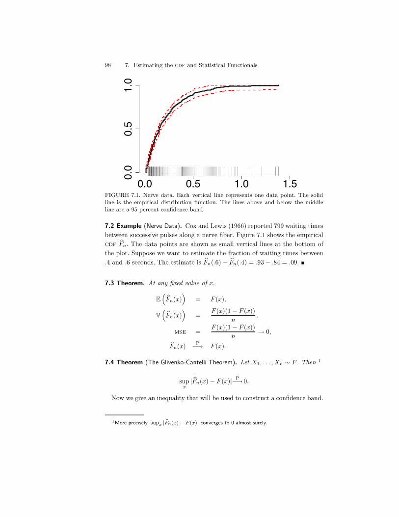
98 7. Estimating the cdf and Statistical Functionals
0.0 0.5 1.0 1.50.0
0.5
1.0
FIGURE 7.1. Nerve data. Each vertical line represents one data point. The solidline is the empirical distribution function. The lines above and below the middleline are a 95 percent confidence band.
7.2 Example (Nerve Data). Cox and Lewis (1966) reported 799 waiting timesbetween successive pulses along a nerve fiber. Figure 7.1 shows the empiricalcdf 1Fn. The data points are shown as small vertical lines at the bottom ofthe plot. Suppose we want to estimate the fraction of waiting times between.4 and .6 seconds. The estimate is 1Fn(.6)" 1Fn(.4) = .93" .84 = .09. !
7.3 Theorem. At any fixed value of x,
E+1Fn(x)
,= F (x),
V+1Fn(x)
,=
F (x)(1 " F (x))n
,
mse =F (x)(1 " F (x))
n) 0,
1Fn(x) P") F (x).
7.4 Theorem (The Glivenko-Cantelli Theorem). Let X1, . . . , Xn ! F . Then 1
supx
| 1Fn(x)" F (x)| P") 0.
Now we give an inequality that will be used to construct a confidence band.
1More precisely, supx | 1Fn(x) " F (x)| converges to 0 almost surely.
7.2 Statistical Functionals 99
7.5 Theorem (The Dvoretzky-Kiefer-Wolfowitz (DKW) Inequality). Let X1, . . .,Xn ! F . Then, for any - > 0,
P(
supx
|F (x) " 1Fn(x)| > -
), 2e$2n&2 . (7.2)
From the DKW inequality, we can construct a confidence set as follows:
A Nonparametric 1" ) Confidence Band for F
Define,
L(x) = max{ 1Fn(x)" -n, 0}U(x) = min{ 1Fn(x) + -n, 1}
where -n =
T12n
log-
2)
..
It follows from (7.2) that for any F ,
P-
L(x) , F (x) , U(x) for all x
.* 1" ). (7.3)
7.6 Example. The dashed lines in Figure 7.1 give a 95 percent confidenceband using -n =
V12n log
;2
.05
<= .048. !
7.2 Statistical Functionals
A statistical functional T (F ) is any function of F . Examples are the meanµ =
8xdF (x), the variance #2 =
8(x " µ)2 dF (x) and the median m =
F$1(1/2).
7.7 Definition. The plug-in estimator of 0 = T (F ) is defined by
10n = T ( 1Fn).
In other words, just plug in 1Fn for the unknown F .
7.8 Definition. If T (F ) =8
r(x)dF (x) for some function r(x) then T iscalled a linear functional.
100 7. Estimating the cdf and Statistical Functionals
The reason T (F ) =8
r(x)dF (x) is called a linear functional is because T
satisfiesT (aF + bG) = aT (F ) + bT (G),
hence T is linear in its arguments. Recall that8
r(x)dF (x) is defined to be8r(x)f(x)dx in the continuous case and
0j r(xj)f(xj) in the discrete. The
empirical cdf 1Fn(x) is discrete, putting mass 1/n at each Xi. Hence, if T (F ) =8r(x)dF (x) is a linear functional then we have:
7.9 Theorem. The plug-in estimator for linear functionalT (F ) =
8r(x)dF (x) is:
T ( 1Fn) =9
r(x)d 1Fn(x) =1n
n*
i=1
r(Xi). (7.4)
Sometimes we can find the estimated standard error se of T ( 1Fn) by doingsome calculations. However, in other cases it is not obvious how to estimatethe standard error. In the next chapter, we will discuss a general method forfinding 1se. For now, let us just assume that somehow we can find 1se.
In many cases, it turns out that
T ( 1Fn) . N(T (F ), 1se2). (7.5)
By equation (6.11), an approximate 1") confidence interval for T (F ) is then
T ( 1Fn) ± z#/2 1se. (7.6)
We will call this the Normal-based interval. For a 95 percent confidenceinterval, z#/2 = z.05/2 = 1.96 . 2 so the interval is
T ( 1Fn) ± 2 1se.
7.10 Example (The mean). Let µ = T (F ) =8
xdF (x). The plug-in estima-
tor is 1µ =8
xd 1Fn(x) = Xn. The standard error is se =V
V(Xn) = #//
n. If1# denotes an estimate of #, then the estimated standard error is 1#/
/n. (In
the next example, we shall see how to estimate #.) A Normal-based confidenceinterval for µ is Xn ± z#/2 1se. !
7.11 Example (The Variance). Let #2 = T (F ) = V(X) =8
x2dF (x)";8
xdF (x)<2.
The plug-in estimator is
1#2 =9
x2d 1Fn(x)"-9
xd 1Fn(x).2
7.2 Statistical Functionals 101
=1n
n*
i=1
X2i "(
1n
n*
i=1
Xi
)2
=1n
n*
i=1
(Xi "Xn)2.
Another reasonable estimator of #2 is the sample variance
S2n =
1n" 1
n*
i=1
(Xi "Xn)2.
In practice, there is little di!erence between 1#2 and S2n and you can use either
one. Returning to the last example, we now see that the estimated standarderror of the estimate of the mean is 1se = 1#/
/n. !
7.12 Example (The Skewness). Let µ and #2 denote the mean and varianceof a random variable X . The skewness is defined to be
1 =E(X " µ)3
#3=
8(x" µ)3dF (x)
Z8(x " µ)2dF (x)
[3/2.
The skewness measures the lack of symmetry of a distribution. To find theplug-in estimate, first recall that 1µ = n$1
0i Xi and 1#2 = n$1
0i(Xi " 1µ)2.
The plug-in estimate of 1 is
11 =8(x" µ)3d 1Fn(x)
!8(x" µ)2d 1Fn(x)
"3/2=
1n
0i(Xi " 1µ)3
1#3. !
7.13 Example (Correlation). Let Z = (X, Y ) and let + = T (F ) = E(X "µX)(Y "µY )/(#x#y) denote the correlation between X and Y , where F (x, y)is bivariate. We can write
T (F ) = a(T1(F ), T2(F ), T3(F ), T4(F ), T5(F ))
where
T1(F ) =8
xdF (z), T2(F ) =8
y dF (z), T3(F ) =8
xy dF (z),T4(F ) =
8x2 dF (z), T5(F ) =
8y2 dF (z),
anda(t1, . . . , t5) =
t3 " t1t23(t4 " t21)(t5 " t22)
.
Replace F with 1Fn in T1(F ), . . . , T5(F ), and take
1+ = a(T1( 1Fn), T2( 1Fn), T3( 1Fn), T4( 1Fn), T5( 1Fn)).
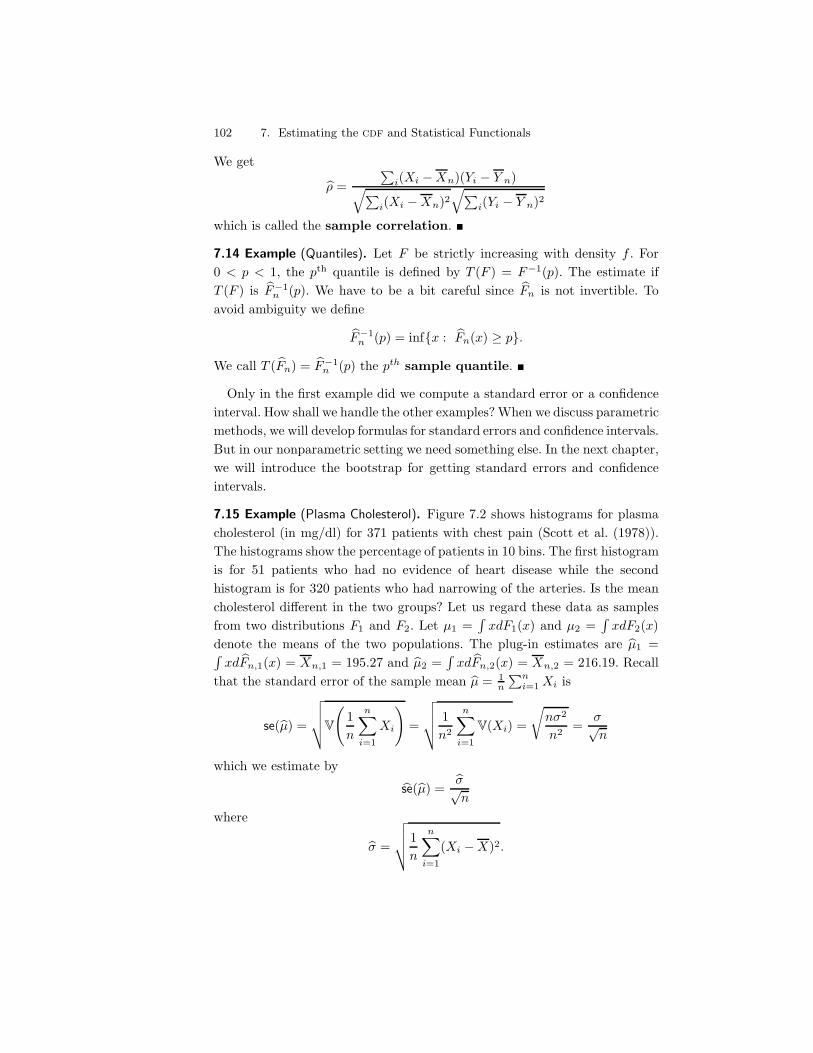
102 7. Estimating the cdf and Statistical Functionals
We get
1+ =0
i(Xi "Xn)(Yi " Y n)V0i(Xi "Xn)2
V0i(Yi " Y n)2
which is called the sample correlation. !
7.14 Example (Quantiles). Let F be strictly increasing with density f . For0 < p < 1, the pth quantile is defined by T (F ) = F$1(p). The estimate ifT (F ) is 1F$1
n (p). We have to be a bit careful since 1Fn is not invertible. Toavoid ambiguity we define
1F$1n (p) = inf{x : 1Fn(x) * p}.
We call T ( 1Fn) = 1F$1n (p) the pth sample quantile. !
Only in the first example did we compute a standard error or a confidenceinterval. How shall we handle the other examples? When we discuss parametricmethods, we will develop formulas for standard errors and confidence intervals.But in our nonparametric setting we need something else. In the next chapter,we will introduce the bootstrap for getting standard errors and confidenceintervals.
7.15 Example (Plasma Cholesterol). Figure 7.2 shows histograms for plasmacholesterol (in mg/dl) for 371 patients with chest pain (Scott et al. (1978)).The histograms show the percentage of patients in 10 bins. The first histogramis for 51 patients who had no evidence of heart disease while the secondhistogram is for 320 patients who had narrowing of the arteries. Is the meancholesterol di!erent in the two groups? Let us regard these data as samplesfrom two distributions F1 and F2. Let µ1 =
8xdF1(x) and µ2 =
8xdF2(x)
denote the means of the two populations. The plug-in estimates are 1µ1 =8xd 1Fn,1(x) = Xn,1 = 195.27 and 1µ2 =
8xd 1Fn,2(x) = Xn,2 = 216.19. Recall
that the standard error of the sample mean 1µ = 1n
0ni=1 Xi is
se(1µ) =
\]]V(
1n
n*
i=1
Xi
)=
\]] 1n2
n*
i=1
V(Xi) =
Un#2
n2=
#/n
which we estimate by
1se(1µ) =1#/n
where
1# =
\]] 1n
n*
i=1
(Xi "X)2.
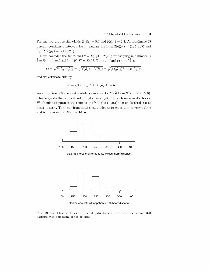
7.2 Statistical Functionals 103
For the two groups this yields 1se(1µ1) = 5.0 and 1se(1µ2) = 2.4. Approximate 95percent confidence intervals for µ1 and µ2 are 1µ1 ± 21se(1µ1) = (185, 205) and1µ2 ± 21se(1µ2) = (211, 221).
Now, consider the functional 0 = T (F2)" T (F1) whose plug-in estimate is10 = 1µ2 " 1µ1 = 216.19" 195.27 = 20.92. The standard error of 10 is
se =3
V(1µ2 " 1µ1) =3
V(1µ2) + V(1µ1) =3
(se(1µ1))2 + (se(1µ2))2
and we estimate this by
1se =3
(1se(1µ1))2 + (1se(1µ2))2 = 5.55.
An approximate 95 percent confidence interval for 0 is 10±2 1se(10n) = (9.8, 32.0).This suggests that cholesterol is higher among those with narrowed arteries.We should not jump to the conclusion (from these data) that cholesterol causesheart disease. The leap from statistical evidence to causation is very subtleand is discussed in Chapter 16. !
plasma cholesterol for patients without heart disease
100 150 200 250 300 350 400
plasma cholesterol for patients with heart disease
100 150 200 250 300 350 400
FIGURE 7.2. Plasma cholesterol for 51 patients with no heart disease and 320patients with narrowing of the arteries.
104 7. Estimating the cdf and Statistical Functionals
7.3 Bibliographic Remarks
The Glivenko-Cantelli theorem is the tip of the iceberg. The theory of dis-tribution functions is a special case of what are called empirical processeswhich underlie much of modern statistical theory. Some references on empiri-cal processes are Shorack and Wellner (1986) and van der Vaart and Wellner(1996).
7.4 Exercises
1. Prove Theorem 7.3.
2. Let X1, . . . , Xn ! Bernoulli(p) and let Y1, . . . , Ym ! Bernoulli(q). Findthe plug-in estimator and estimated standard error for p. Find an ap-proximate 90 percent confidence interval for p. Find the plug-in esti-mator and estimated standard error for p" q. Find an approximate 90percent confidence interval for p" q.
3. (Computer Experiment.) Generate 100 observations from a N(0,1) dis-tribution. Compute a 95 percent confidence band for the cdf F (asdescribed in the appendix). Repeat this 1000 times and see how oftenthe confidence band contains the true distribution function. Repeat us-ing data from a Cauchy distribution.
4. Let X1, . . . , Xn ! F and let 1Fn(x) be the empirical distribution func-tion. For a fixed x, use the central limit theorem to find the limitingdistribution of 1Fn(x).
5. Let x and y be two distinct points. Find Cov( 1Fn(x), 1Fn(y)).
6. Let X1, . . . , Xn ! F and let 1F be the empirical distribution function.Let a < b be fixed numbers and define 0 = T (F ) = F (b) " F (a). Let10 = T ( 1Fn) = 1Fn(b) " 1Fn(a). Find the estimated standard error of 10.Find an expression for an approximate 1" ) confidence interval for 0.
7. Data on the magnitudes of earthquakes near Fiji are available on thewebsite for this book. Estimate the cdf F (x). Compute and plot a 95percent confidence envelope for F (as described in the appendix). Findan approximate 95 percent confidence interval for F (4.9)" F (4.3).

7.4 Exercises 105
8. Get the data on eruption times and waiting times between eruptions ofthe Old Faithful geyser from the website. Estimate the mean waitingtime and give a standard error for the estimate. Also, give a 90 percentconfidence interval for the mean waiting time. Now estimate the medianwaiting time. In the next chapter we will see how to get the standarderror for the median.
9. 100 people are given a standard antibiotic to treat an infection andanother 100 are given a new antibiotic. In the first group, 90 peoplerecover; in the second group, 85 people recover. Let p1 be the probabilityof recovery under the standard treatment and let p2 be the probability ofrecovery under the new treatment. We are interested in estimating 0 =p1 " p2. Provide an estimate, standard error, an 80 percent confidenceinterval, and a 95 percent confidence interval for 0.
10. In 1975, an experiment was conducted to see if cloud seeding producedrainfall. 26 clouds were seeded with silver nitrate and 26 were not. Thedecision to seed or not was made at random. Get the data from
http://lib.stat.cmu.edu/DASL/Stories/CloudSeeding.html
Let 0 be the di!erence in the mean precipitation from the two groups.Estimate 0. Estimate the standard error of the estimate and produce a95 percent confidence interval.

This is page 106Printer: Opaque this
This is page 107Printer: Opaque this
8The Bootstrap
The bootstrap is a method for estimating standard errors and computingconfidence intervals. Let Tn = g(X1, . . . , Xn) be a statistic, that is, Tn is anyfunction of the data. Suppose we want to know VF (Tn), the variance of Tn.We have written VF to emphasize that the variance usually depends on theunknown distribution function F . For example, if Tn = Xn then VF (Tn) =#2/n where #2 =
8(x"µ)2dF (x) and µ =
8xdF (x). Thus the variance of Tn
is a function of F . The bootstrap idea has two steps:
Step 1: Estimate VF (Tn) with V 1Fn(Tn).
Step 2: Approximate V 1Fn(Tn) using simulation.
For Tn = Xn, we have for Step 1 that V 1Fn(Tn) = 1#2/n where 1#2 = n$1
0ni=1(Xi"
Xn). In this case, Step 1 is enough. However, in more complicated cases wecannot write down a simple formula for V 1Fn
(Tn) which is why we need Step2. Before proceeding, let us discuss the idea of simulation.
108 8. The Bootstrap
8.1 Simulation
Suppose we draw an iid sample Y1, . . . , YB from a distribution G. By the lawof large numbers,
Y n =1B
B*
j=1
YjP")9
y dG(y) = E(Y )
as B ) #. So if we draw a large sample from G, we can use the samplemean Y n to approximate E(Y ). In a simulation, we can make B as large aswe like, in which case, the di!erence between Y n and E(Y ) is negligible. Moregenerally, if h is any function with finite mean then
1B
B*
j=1
h(Yj)P")9
h(y)dG(y) = E(h(Y ))
as B )#. In particular,
1B
B*
j=1
(Yj " Y )2 =1B
B*
j=1
Y 2j "
(1B
B*
j=1
Yj
)2
P")9
y2dF (y)"(9
ydF (y)
)2
= V(Y ).
Hence, we can use the sample variance of the simulated values to approximateV(Y ).
8.2 Bootstrap Variance Estimation
According to what we just learned, we can approximate V 1Fn(Tn) by simula-
tion. Now V 1Fn(Tn) means “the variance of Tn if the distribution of the data
is 1Fn.” How can we simulate from the distribution of Tn when the data areassumed to have distribution 1Fn? The answer is to simulate X*
1 , . . . , X*n from
1Fn and then compute T *n = g(X*
1 , . . . , X*n). This constitutes one draw from
the distribution of Tn. The idea is illustrated in the following diagram:
Real world F =+ X1, . . . , Xn =+ Tn = g(X1, . . . , Xn)Bootstrap world 1Fn =+ X*
1 , . . . , X*n =+ T *
n = g(X*1 , . . . , X*
n)
How do we simulate X*1 , . . . , X*
n from 1Fn? Notice that 1Fn puts mass 1/n ateach data point X1, . . . , Xn. Therefore,
8.2 Bootstrap Variance Estimation 109
drawing an observation from 1Fn is equivalent to drawingone point at random from the original data set.
Thus, to simulate X*1 , . . . , X*
n ! 1Fn it su#ces to draw n observations withreplacement from X1, . . . , Xn. Here is a summary:
Bootstrap Variance Estimation
1. Draw X*1 , . . . , X*
n ! 1Fn.
2. Compute T *n = g(X*
1 , . . . , X*n).
3. Repeat steps 1 and 2, B times, to get T *n,1, . . . , T
*n,B.
4. Let
vboot =1B
B*
b=1
(T *
n,b "1B
B*
r=1
T *n,r
)2
. (8.1)
8.1 Example. The following pseudocode shows how to use the bootstrap toestimate the standard error of the median.
Bootstrap for The Median
Given data X = (X(1), ..., X(n)):
T <- median(X)
Tboot <- vector of length B
for(i in 1:B){
Xstar <- sample of size n from X (with replacement)
Tboot[i] <- median(Xstar)
}
se <- sqrt(variance(Tboot))
The following schematic diagram will remind you that we are using twoapproximations:
VF (Tn)not so small_`ab. V 1Fn
(Tn)small_`ab. vboot.
8.2 Example. Consider the nerve data. Let 0 = T (F ) =8(x"µ)3dF (x)/#3 be
the skewness. The skewness is a measure of asymmetry. A Normal distribution,
110 8. The Bootstrap
for example, has skewness 0. The plug-in estimate of the skewness is
10 = T ( 1Fn) =8
(x" µ)3d 1Fn(x)1#3
=1n
0ni=1(Xi "Xn)3
1#3= 1.76.
To estimate the standard error with the bootstrap we follow the same stepsas with the median example except we compute the skewness from eachbootstrap sample. When applied to the nerve data, the bootstrap, based onB = 1, 000 replications, yields a standard error for the estimated skewness of.16. !
8.3 Bootstrap Confidence Intervals
There are several ways to construct bootstrap confidence intervals. Here wediscuss three methods.
Method 1: The Normal Interval. The simplest method is the Normal interval
Tn ± z#/2 1seboot (8.2)
where 1seboot =/
vboot is the bootstrap estimate of the standard error. Thisinterval is not accurate unless the distribution of Tn is close to Normal.
Method 2: Pivotal Intervals. Let 0 = T (F ) and 10n = T ( 1Fn) and define thepivot Rn = 10n" 0. Let 10*n,1, . . . , 10*n,B denote bootstrap replications of 10n. LetH(r) denote the cdf of the pivot:
H(r) = PF (Rn , r). (8.3)
Define C)n = (a, b) where
a = 10n "H$1+1" )
2
,and b = 10n "H$1
+)2
,. (8.4)
It follows that
P(a , 0 , b) = P(a" 10n , 0 " 10n , b" 10n)
= P(10n " b , 10n " 0 , 10n " a)
= P(10n " b , Rn , 10n " a)
= H(10n " a)"H(10n " b)
= H+H$1
+1" )
2
,,"H
+H$1
+)2
,,
= 1" )
2" )
2= 1" ).
8.3 Bootstrap Confidence Intervals 111
Hence, C)n is an exact 1" ) confidence interval for 0. Unfortunately, a and b
depend on the unknown distribution H but we can form a bootstrap estimateof H :
1H(r) =1B
B*
b=1
I(R*n,b , r) (8.5)
where R*n,b = 10*n,b"10n. Let r*" denote the ( sample quantile of (R*
n,1, . . . , R*n,B)
and let 0*" denote the ( sample quantile of (10*n,1, . . . , 10*n,B). Note that r*" =0*"" 10n. It follows that an approximate 1") confidence interval is Cn = (1a,1b)where
1a = 10n " 1H$1+1" )
2
,= 10n " r*1$#/2 = 210n " 0*1$#/2
1b = 10n " 1H$1+)
2
,= 10n " r*#/2 = 210n " 0*#/2.
In summary, the 1" ) bootstrap pivotal confidence interval is
Cn =+210n " 10*1$#/2, 210n " 10*#/2
,. (8.6)
8.3 Theorem. Under weak conditions on T (F ),
PF (T (F ) $ Cn)) 1" )
as n)#, where Cn is given in (8.6).
Method 3: Percentile Intervals. The bootstrap percentile interval is de-fined by
Cn =+0*#/2, 0
*1$#/2
,.
The justification for this interval is given in the appendix.
8.4 Example. For estimating the skewness of the nerve data, here are thevarious confidence intervals.
Method 95% IntervalNormal (1.44, 2.09)Pivotal (1.48, 2.11)Percentile (1.42, 2.03)
All these confidence intervals are approximate. The probability that T (F )is in the interval is not exactly 1" ). All three intervals have the same levelof accuracy. There are more accurate bootstrap confidence intervals but theyare more complicated and we will not discuss them here.
112 8. The Bootstrap
8.5 Example (The Plasma Cholesterol Data). Let us return to the cholesteroldata. Suppose we are interested in the di!erence of the medians. Pseudocodefor the bootstrap analysis is as follows:
x1 <- first sample
x2 <- second sample
n1 <- length(x1)
n2 <- length(x2)
th.hat <- median(x2) - median(x1)
B <- 1000
Tboot <- vector of length B
for(i in 1:B){
xx1 <- sample of size n1 with replacement from x1
xx2 <- sample of size n2 with replacement from x2
Tboot[i] <- median(xx2) - median(xx1)
}
se <- sqrt(variance(Tboot))
Normal <- (th.hat - 2*se, th.hat + 2*se)
percentile <- (quantile(Tboot,.025), quantile(Tboot,.975))
pivotal <- ( 2*th.hat-quantile(Tboot,.975),
2*th.hat-quantile(Tboot,.025) )
The point estimate is 18.5, the bootstrap standard error is 7.42 and the re-sulting approximate 95 percent confidence intervals are as follows:
Method 95% IntervalNormal (3.7, 33.3)Pivotal (5.0, 34.0)Percentile (5.0, 33.3)
Since these intervals exclude 0, it appears that the second group has highercholesterol although there is considerable uncertainty about how much higheras reflected in the width of the intervals. !
The next two examples are based on small sample sizes. In practice, sta-tistical methods based on very small sample sizes might not be reliable. Weinclude the examples for their pedagogical value but we do want to sound anote of caution about interpreting the results with some skepticism.
8.6 Example. Here is an example that was one of the first used to illustratethe bootstrap by Bradley Efron, the inventor of the bootstrap. The data areLSAT scores (for entrance to law school) and GPA.
8.3 Bootstrap Confidence Intervals 113
LSAT 576 635 558 578 666 580 555 661
651 605 653 575 545 572 594
GPA 3.39 3.30 2.81 3.03 3.44 3.07 3.00 3.43
3.36 3.13 3.12 2.74 2.76 2.88 3.96
Each data point is of the form Xi = (Yi, Zi) where Yi = LSATi and Zi =GPAi. The law school is interested in the correlation
0 =8 8
(y " µY )(z " µZ)dF (y, z)V8(y " µY )2dF (y)
8(z " µZ)2dF (z)
.
The plug-in estimate is the sample correlation
10 =0
i(Yi " Y )(Zi " Z)V0i(Yi " Y )2
0i(Zi " Z)2
.
The estimated correlation is 10 = .776. The bootstrap based on B = 1000gives 1se = .137. Figure 8.1 shows the data and a histogram of the bootstrapreplications 10*1 , . . . , 10*B. This histogram is an approximation to the samplingdistribution of 10. The Normal-based 95 percent confidence interval is .78 ±21se = (.51, 1.00) while the percentile interval is (.46,.96). In large samples, thetwo methods will show closer agreement. !
8.7 Example. This example is from Efron and Tibshirani (1993). When drugcompanies introduce new medications, they are sometimes required to showbioequivalence. This means that the new drug is not substantially di!erentthan the current treatment. Here are data on eight subjects who used medi-cal patches to infuse a hormone into the blood. Each subject received threetreatments: placebo, old-patch, new-patch.
subject placebo old new old " placebo new " old1 9243 17649 16449 8406 -12002 9671 12013 14614 2342 26013 11792 19979 17274 8187 -27054 13357 21816 23798 8459 19825 9055 13850 12560 4795 -12906 6290 9806 10157 3516 3517 12412 17208 16570 4796 -6388 18806 29044 26325 10238 -2719
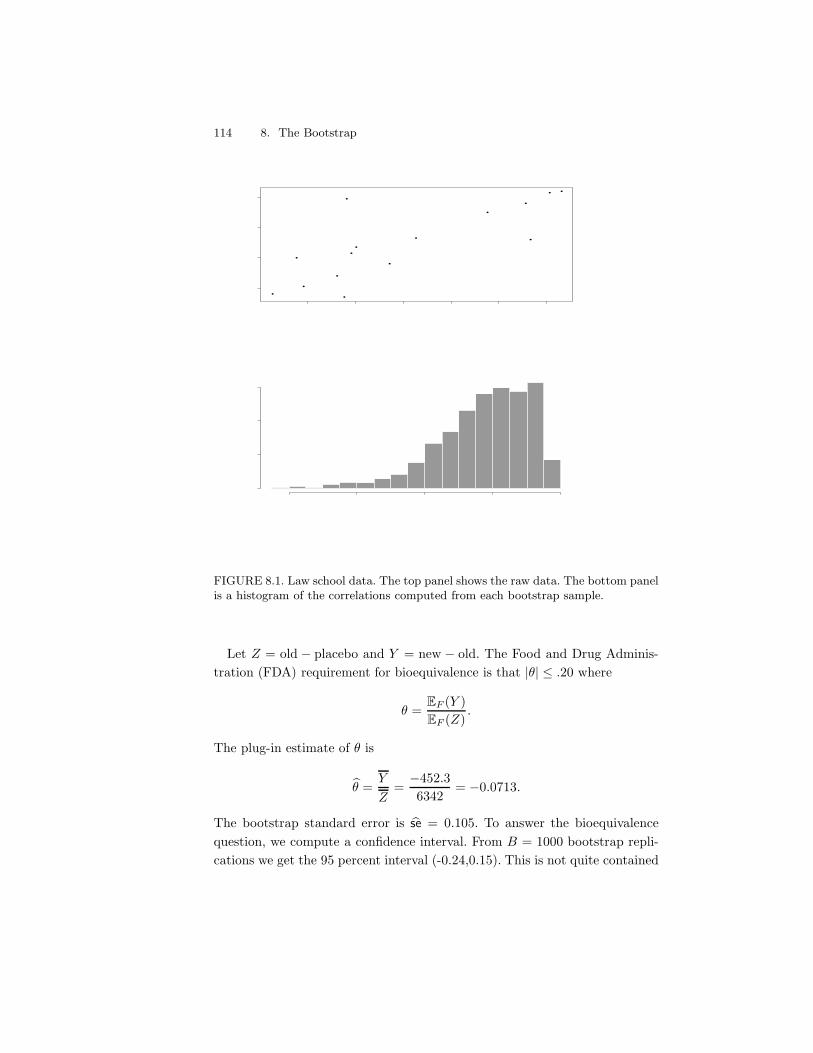
114 8. The Bootstrap
•
•
•
•
•
••
••
• •
••
••
FIGURE 8.1. Law school data. The top panel shows the raw data. The bottom panelis a histogram of the correlations computed from each bootstrap sample.
Let Z = old " placebo and Y = new " old. The Food and Drug Adminis-tration (FDA) requirement for bioequivalence is that |0| , .20 where
0 =EF (Y )EF (Z)
.
The plug-in estimate of 0 is
10 =Y
Z="452.36342
= "0.0713.
The bootstrap standard error is 1se = 0.105. To answer the bioequivalencequestion, we compute a confidence interval. From B = 1000 bootstrap repli-cations we get the 95 percent interval (-0.24,0.15). This is not quite contained
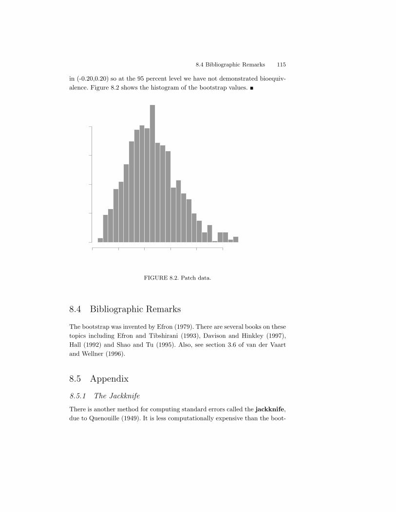
8.4 Bibliographic Remarks 115
in (-0.20,0.20) so at the 95 percent level we have not demonstrated bioequiv-alence. Figure 8.2 shows the histogram of the bootstrap values. !
FIGURE 8.2. Patch data.
8.4 Bibliographic Remarks
The bootstrap was invented by Efron (1979). There are several books on thesetopics including Efron and Tibshirani (1993), Davison and Hinkley (1997),Hall (1992) and Shao and Tu (1995). Also, see section 3.6 of van der Vaartand Wellner (1996).
8.5 Appendix
8.5.1 The Jackknife
There is another method for computing standard errors called the jackknife,due to Quenouille (1949). It is less computationally expensive than the boot-
116 8. The Bootstrap
strap but is less general. Let Tn = T (X1, . . . , Xn) be a statistic and T($i) de-note the statistic with the ith observation removed. Let Tn = n$1
0ni=1 T($i).
The jackknife estimate of var(Tn) is
vjack =n" 1
n
n*
i=1
(T($i) " Tn)2
and the jackknife estimate of the standard error is 1sejack = /vjack. Undersuitable conditions on T , it can be shown that vjack consistently estimatesvar(Tn) in the sense that vjack/var(Tn)
P") 1. However, unlike the bootstrap,the jackknife does not produce consistent estimates of the standard error ofsample quantiles.
8.5.2 Justification For The Percentile Interval
Suppose there exists a monotone transformation U = m(T ) such that U !N(', c2) where ' = m(0). We do not suppose we know the transformation,only that one exists. Let U*
b = m(0*n,b). Let u*" be the ( sample quantile of
the U*b ’s. Since a monotone transformation preserves quantiles, we have that
u*#/2 = m(0*#/2). Also, since U ! N(', c2), the )/2 quantile of U is '" z#/2c.
Hence u*#/2 = '" z#/2c. Similarly, u*
1$#/2 = '+ z#/2c. Therefore,
P(0*#/2 , 0 , 0*1$#/2) = P(m(0*#/2) , m(0) , m(0*1$#/2))
= P(u*#/2 , ' , u*
1$#/2)
= P(U " cz#/2 , ' , U + cz#/2)
= P("z#/2 ,U " '
c, z#/2)
= 1" ).
An exact normalizing transformation will rarely exist but there may existapproximate normalizing transformations.
8.6 Exercises
1. Consider the data in Example 8.6. Find the plug-in estimate of thecorrelation coe#cient. Estimate the standard error using the bootstrap.Find a 95 percent confidence interval using the Normal, pivotal, andpercentile methods.
8.6 Exercises 117
2. (Computer Experiment.) Conduct a simulation to compare the variousbootstrap confidence interval methods. Let n = 50 and let T (F ) =8(x " µ)3dF (x)/#3 be the skewness. Draw Y1, . . . , Yn ! N(0, 1) and
set Xi = eYi , i = 1, . . . , n. Construct the three types of bootstrap 95percent intervals for T (F ) from the data X1, . . . , Xn. Repeat this wholething many times and estimate the true coverage of the three intervals.
3. LetX1, . . . , Xn ! t3
where n = 25. Let 0 = T (F ) = (q.75 " q.25)/1.34 where qp denotes thepth quantile. Do a simulation to compare the coverage and length of thefollowing confidence intervals for 0: (i) Normal interval with standarderror from the bootstrap, (ii) bootstrap percentile interval, and (iii)pivotal bootstrap interval.
4. Let X1, . . . , Xn be distinct observations (no ties). Show that there are-
2n" 1n
.
distinct bootstrap samples.
Hint: Imagine putting n balls into n buckets.
5. Let X1, . . . , Xn be distinct observations (no ties). Let X*1 , . . . , X*
n denotea bootstrap sample and let X
*n = n$1
0ni=1 X*
i . Find: E(X*n|X1, . . . , Xn),
V(X*n|X1, . . . , Xn), E(X*
n) and V(X*n).
6. (Computer Experiment.) Let X1, ..., Xn Normal(µ, 1). Let 0 = eµ and let10 = eX . Create a data set (using µ = 5) consisting of n=100 observa-tions.
(a) Use the bootstrap to get the se and 95 percent confidence intervalfor 0.
(b) Plot a histogram of the bootstrap replications. This is an estimateof the distribution of 10. Compare this to the true sampling distributionof 10.
7. Let X1, ..., Xn ! Uniform(0, 0). Let 10 = Xmax = max{X1, ..., Xn}. Gen-erate a data set of size 50 with 0 = 1.
(a) Find the distribution of 10. Compare the true distribution of 10 to thehistograms from the bootstrap.
118 8. The Bootstrap
(b) This is a case where the bootstrap does very poorly. In fact, we canprove that this is the case. Show that P (10 = 10) = 0 and yet P (10* =10) . .632. Hint: show that, P (10* = 10) = 1" (1" (1/n))n then take thelimit as n gets large.
8. Let Tn = X2n, µ = E(X1), )k =
8|x"µ|kdF (x) and 1)k = n$1
0ni=1 |Xi"
Xn|k. Show that
vboot =4X
2n1)2
n+
4Xn1)3
n2+1)4
n3.
This is page 119Printer: Opaque this
9Parametric Inference
We now turn our attention to parametric models, that is, models of the form
F ='
f(x; 0) : 0 $ "2
(9.1)
where the " & Rk is the parameter space and 0 = (01, . . . , 0k) is the param-eter. The problem of inference then reduces to the problem of estimating theparameter 0.
Students learning statistics often ask: how would we ever know that thedistribution that generated the data is in some parametric model? This isan excellent question. Indeed, we would rarely have such knowledge whichis why nonparametric methods are preferable. Still, studying methods forparametric models is useful for two reasons. First, there are some cases wherebackground knowledge suggests that a parametric model provides a reasonableapproximation. For example, counts of tra#c accidents are known from priorexperience to follow approximately a Poisson model. Second, the inferentialconcepts for parametric models provide background for understanding certainnonparametric methods.
We begin with a brief discussion about parameters of interest and nuisanceparameters in the next section, then we will discuss two methods for estimat-ing 0, the method of moments and the method of maximum likelihood.
120 9. Parametric Inference
9.1 Parameter of Interest
Often, we are only interested in some function T (0). For example, if X !N(µ,#2) then the parameter is 0 = (µ,#). If our goal is to estimate µ thenµ = T (0) is called the parameter of interest and # is called a nuisanceparameter. The parameter of interest might be a complicated function of 0as in the following example.
9.1 Example. Let X1, . . . , Xn ! Normal(µ,#2). The parameter is 0 = (µ,#)and the parameter space is " = {(µ,#) : µ $ R, # > 0}. Suppose that Xi isthe outcome of a blood test and suppose we are interested in 2 , the fractionof the population whose test score is larger than 1. Let Z denote a standardNormal random variable. Then
2 = P(X > 1) = 1" P(X < 1) = 1" P-
X " µ
#<
1" µ
#
.
= 1" P-
Z <1" µ
#
.= 1" %
-1" µ
#
..
The parameter of interest is 2 = T (µ,#) = 1" %((1" µ)/#). !
9.2 Example. Recall that X has a Gamma(),() distribution if
f(x; ),() =1
(#&())x#$1e$x/", x > 0
where ),( > 0 and
&()) =9 !
0y#$1e$ydy
is the Gamma function. The parameter is 0 = (),(). The Gamma distri-bution is sometimes used to model lifetimes of people, animals, and elec-tronic equipment. Suppose we want to estimate the mean lifetime. ThenT (),() = E((X1) = )(. !
9.2 The Method of Moments
The first method for generating parametric estimators that we will studyis called the method of moments. We will see that these estimators are notoptimal but they are often easy to compute. They are are also useful as startingvalues for other methods that require iterative numerical routines.
9.2 The Method of Moments 121
Suppose that the parameter 0 = (01, . . . , 0k) has k components. For 1 ,j , k, define the jth moment
)j 0 )j(0) = E((Xj) =9
xjdF((x) (9.2)
and the jth sample moment
1)j =1n
n*
i=1
Xji . (9.3)
9.3 Definition. The method of moments estimator 10n is defined to bethe value of 0 such that
)1(10n) = 1)1
)2(10n) = 1)2
......
...
)k(10n) = 1)k. (9.4)
Formula (9.4) defines a system of k equations with k unknowns.
9.4 Example. Let X1, . . . , Xn ! Bernoulli(p). Then )1 = Ep(X) = p and1)1 = n$1
0ni=1 Xi. By equating these we get the estimator
1pn =1n
n*
i=1
Xi. !
9.5 Example. Let X1, . . . , Xn ! Normal(µ,#2). Then, )1 = E((X1) = µ
and )2 = E((X21 ) = V((X1) + (E((X1))2 = #2 + µ2. We need to solve the
equations1
1µ =1n
n*
i=1
Xi
1#2 + 1µ2 =1n
n*
i=1
X2i .
This is a system of 2 equations with 2 unknowns. The solution is
1µ = Xn
1Recall that V(X) = E(X2) " (E(X))2. Hence, E(X2) = V(X) + (E(X))2.
122 9. Parametric Inference
1#2 =1n
n*
i=1
(Xi "Xn)2. !
9.6 Theorem. Let 10n denote the method of moments estimator. Under appro-priate conditions on the model, the following statements hold:
1. The estimate 10n exists with probability tending to 1.
2. The estimate is consistent: 10nP") 0.
3. The estimate is asymptotically Normal:/
n(10n " 0) ! N(0,')
where' = gE((Y Y T )gT ,
Y = (X, X2, . . . , Xk)T , g = (g1, . . . , gk) and gj = 3)$1j (0)/30.
The last statement in the theorem above can be used to find standard errorsand confidence intervals. However, there is an easier way: the bootstrap. Wedefer discussion of this until the end of the chapter.
9.3 Maximum Likelihood
The most common method for estimating parameters in a parametric model isthe maximum likelihood method. Let X1, . . ., Xn be iid with pdf f(x; 0).
9.7 Definition. The likelihood function is defined by
Ln(0) =n/
i=1
f(Xi; 0). (9.5)
The log-likelihood function is defined by 4n(0) = logLn(0).
The likelihood function is just the joint density of the data, except that wetreat it is a function of the parameter 0. Thus, Ln : " ) [0,#). Thelikelihood function is not a density function: in general, it is not true thatLn(0) integrates to 1 (with respect to 0).
9.8 Definition. The maximum likelihood estimator mle, denoted by10n, is the value of 0 that maximizes Ln(0).
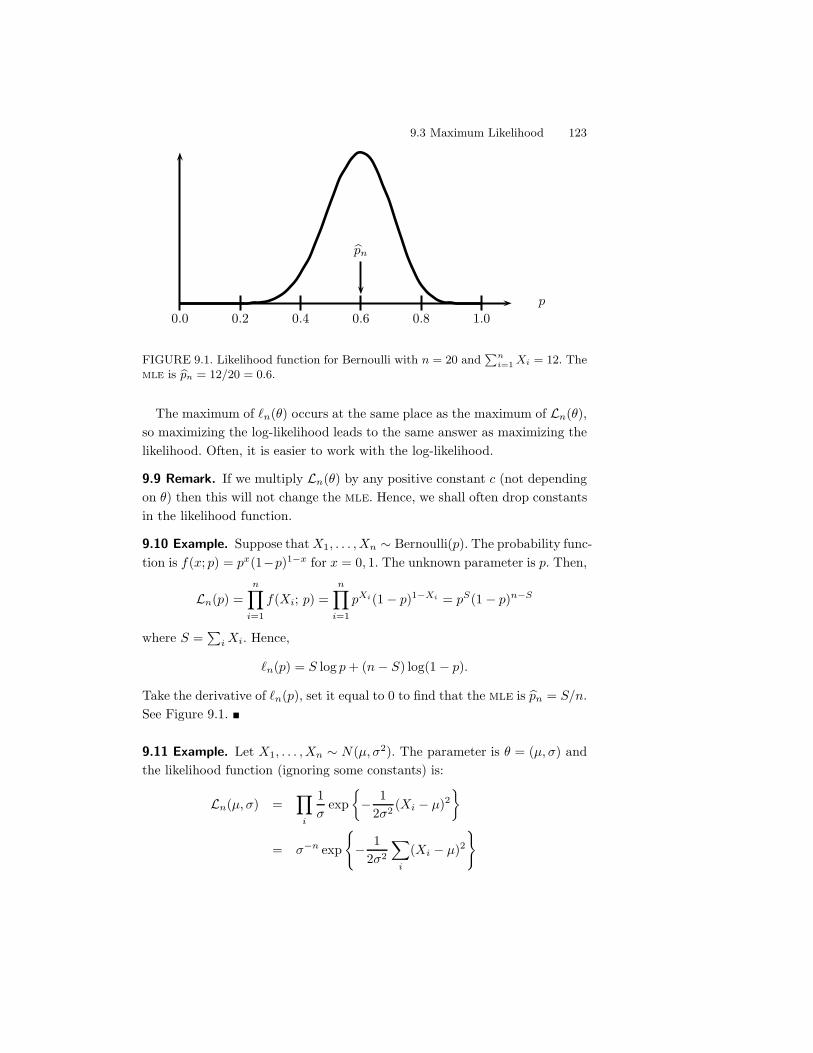
9.3 Maximum Likelihood 123
0.0 0.2 0.4 0.6 0.8 1.0p
1pn
FIGURE 9.1. Likelihood function for Bernoulli with n = 20 and0n
i=1 Xi = 12. Themle is 1pn = 12/20 = 0.6.
The maximum of 4n(0) occurs at the same place as the maximum of Ln(0),so maximizing the log-likelihood leads to the same answer as maximizing thelikelihood. Often, it is easier to work with the log-likelihood.
9.9 Remark. If we multiply Ln(0) by any positive constant c (not dependingon 0) then this will not change the mle. Hence, we shall often drop constantsin the likelihood function.
9.10 Example. Suppose that X1, . . . , Xn ! Bernoulli(p). The probability func-tion is f(x; p) = px(1"p)1$x for x = 0, 1. The unknown parameter is p. Then,
Ln(p) =n/
i=1
f(Xi; p) =n/
i=1
pXi(1" p)1$Xi = pS(1 " p)n$S
where S =0
i Xi. Hence,
4n(p) = S log p + (n" S) log(1" p).
Take the derivative of 4n(p), set it equal to 0 to find that the mle is 1pn = S/n.See Figure 9.1. !
9.11 Example. Let X1, . . . , Xn ! N(µ,#2). The parameter is 0 = (µ,#) andthe likelihood function (ignoring some constants) is:
Ln(µ,#) =/
i
1#
exp'" 1
2#2(Xi " µ)2
2
= #$n exp
:" 1
2#2
*
i
(Xi " µ)2Y
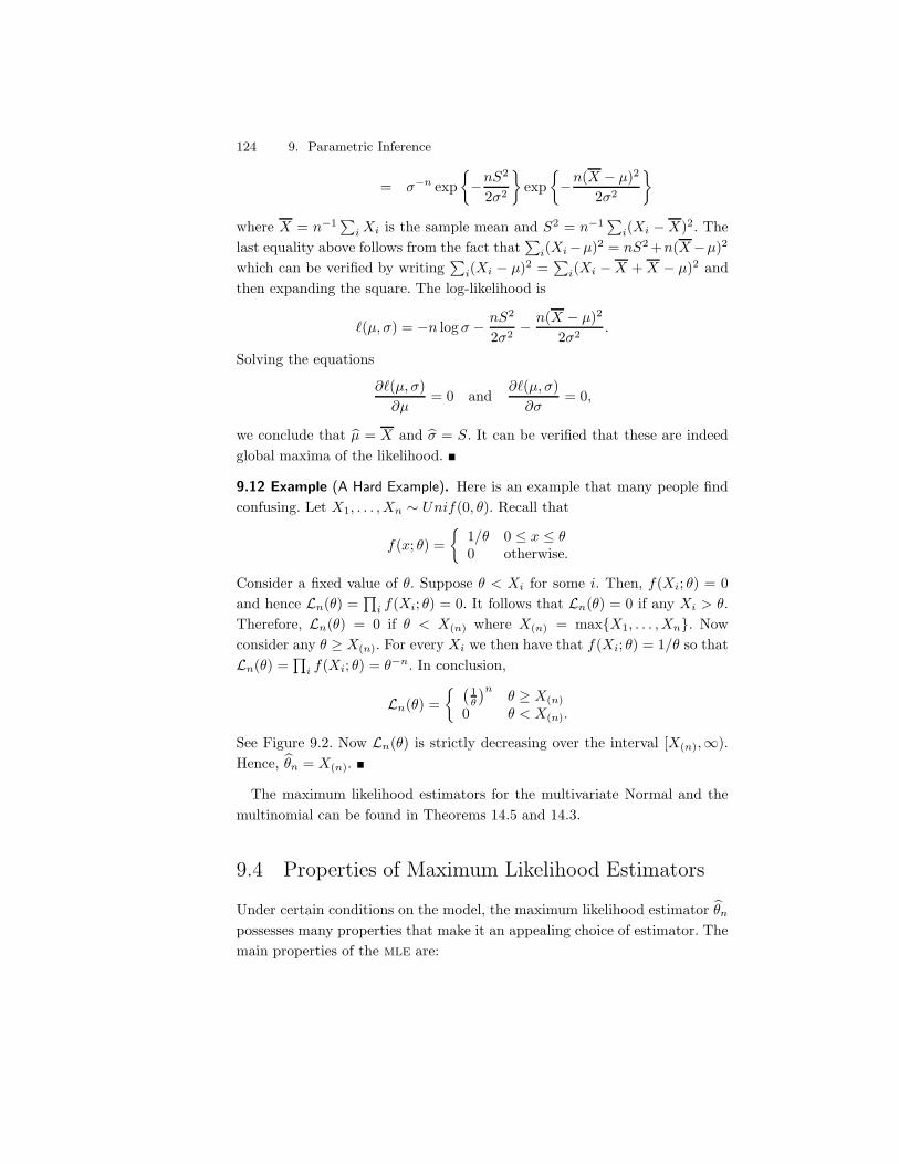
124 9. Parametric Inference
= #$n exp'"nS2
2#2
2exp'"n(X " µ)2
2#2
2
where X = n$10
i Xi is the sample mean and S2 = n$10
i(Xi "X)2. Thelast equality above follows from the fact that
0i(Xi"µ)2 = nS2 +n(X"µ)2
which can be verified by writing0
i(Xi " µ)2 =0
i(Xi "X + X " µ)2 andthen expanding the square. The log-likelihood is
4(µ,#) = "n log# " nS2
2#2" n(X " µ)2
2#2.
Solving the equations
34(µ,#)3µ
= 0 and34(µ,#)3#
= 0,
we conclude that 1µ = X and 1# = S. It can be verified that these are indeedglobal maxima of the likelihood. !
9.12 Example (A Hard Example). Here is an example that many people findconfusing. Let X1, . . . , Xn ! Unif(0, 0). Recall that
f(x; 0) ='
1/0 0 , x , 00 otherwise.
Consider a fixed value of 0. Suppose 0 < Xi for some i. Then, f(Xi; 0) = 0and hence Ln(0) =
Di f(Xi; 0) = 0. It follows that Ln(0) = 0 if any Xi > 0.
Therefore, Ln(0) = 0 if 0 < X(n) where X(n) = max{X1, . . . , Xn}. Nowconsider any 0 * X(n). For every Xi we then have that f(Xi; 0) = 1/0 so thatLn(0) =
Di f(Xi; 0) = 0$n. In conclusion,
Ln(0) =' ;
1(
<n0 * X(n)
0 0 < X(n).
See Figure 9.2. Now Ln(0) is strictly decreasing over the interval [X(n),#).Hence, 10n = X(n). !
The maximum likelihood estimators for the multivariate Normal and themultinomial can be found in Theorems 14.5 and 14.3.
9.4 Properties of Maximum Likelihood Estimators
Under certain conditions on the model, the maximum likelihood estimator 10n
possesses many properties that make it an appealing choice of estimator. Themain properties of the mle are:
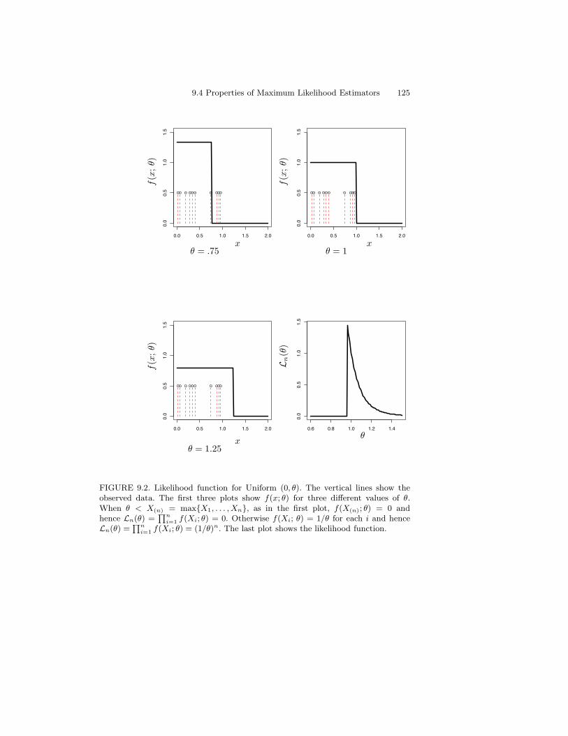
9.4 Properties of Maximum Likelihood Estimators 125
0.0 0.5 1.0 1.5 2.0
0.0
0.5
1.0
1.5
0.0 0.5 1.0 1.5 2.0
0.0
0.5
1.0
1.5
0.0 0.5 1.0 1.5 2.0
0.0
0.5
1.0
1.5
0.6 0.8 1.0 1.2 1.4
0.0
0.5
1.0
1.5
0 = .75 0 = 1
0 = 1.25
x x
x0
f(x
;0)
f(x
;0)
f(x
;0)
L n(0
)
FIGURE 9.2. Likelihood function for Uniform (0, !). The vertical lines show theobserved data. The first three plots show f(x; !) for three di"erent values of !.When ! < X(n) = max{X1, . . . , Xn}, as in the first plot, f(X(n); !) = 0 andhence Ln(!) =
Dni=1 f(Xi; !) = 0. Otherwise f(Xi; !) = 1/! for each i and hence
Ln(!) =Dn
i=1 f(Xi; !) = (1/!)n. The last plot shows the likelihood function.
126 9. Parametric Inference
1. The mle is consistent: 10nP") 0) where 0) denotes the true value of the
parameter 0;
2. The mle is equivariant: if 10n is the mle of 0 then g(10n) is the mle ofg(0);
3. The mle is asymptotically Normal: (10 " 0))/1se ! N(0, 1); also, theestimated standard error 1se can often be computed analytically;
4. The mle is asymptotically optimal or e!cient: roughly, this meansthat among all well-behaved estimators, the mle has the smallest vari-ance, at least for large samples;
5. The mle is approximately the Bayes estimator. (This point will be ex-plained later.)
We will spend some time explaining what these properties mean and whythey are good things. In su#ciently complicated problems, these propertieswill no longer hold and the mle will no longer be a good estimator. For nowwe focus on the simpler situations where the mle works well. The propertieswe discuss only hold if the model satisfies certain regularity conditions.These are essentially smoothness conditions on f(x; 0). Unless otherwisestated, we shall tacitly assume that these conditions hold.
9.5 Consistency of Maximum Likelihood Estimators
Consistency means that the mle converges in probability to the true value.To proceed, we need a definition. If f and g are pdf’s, define the Kullback-Leibler distance 2 between f and g to be
D(f, g) =9
f(x) log-
f(x)g(x)
.dx. (9.6)
It can be shown that D(f, g) * 0 and D(f, f) = 0. For any 0,, $ " writeD(0,,) to mean D(f(x; 0), f(x; ,)).
We will say that the model F is identifiable if 0 (= , implies that D(0,,) >
0. This means that di!erent values of the parameter correspond to di!erentdistributions. We will assume from now on the the model is identifiable.
2This is not a distance in the formal sense because D(f, g) is not symmetric.
9.6 Equivariance of the mle 127
Let 0) denote the true value of 0. Maximizing 4n(0) is equivalent to maxi-mizing
Mn(0) =1n
*
i
logf(Xi; 0)f(Xi; 0))
.
This follows since Mn(0) = n$1(4n(0)" 4n(0))) and 4n(0)) is a constant (withrespect to 0). By the law of large numbers, Mn(0) converges to
E(!
(log
f(Xi; 0)f(Xi; 0))
)=
9log-
f(x; 0)f(x; 0))
.f(x; 0))dx
= "9
log-
f(x; 0))f(x; 0)
.f(x; 0))dx
= "D(0), 0).
Hence, Mn(0) . "D(0), 0) which is maximized at 0) since "D(0), 0)) = 0and "D(0), 0) < 0 for 0 (= 0). Therefore, we expect that the maximizer willtend to 0). To prove this formally, we need more than Mn(0) P") "D(0), 0).We need this convergence to be uniform over 0. We also have to make surethat the function D(0), 0) is well behaved. Here are the formal details.
9.13 Theorem. Let 0) denote the true value of 0. Define
Mn(0) =1n
*
i
logf(Xi; 0)f(Xi; 0))
and M(0) = "D(0), 0). Suppose that
sup(#!
|Mn(0)"M(0)| P") 0 (9.7)
and that, for every - > 0,
sup(:|($(!|+&
M(0) < M(0)). (9.8)
Let 10n denote the mle. Then 10nP") 0).
The proof is in the appendix.
9.6 Equivariance of the mle
9.14 Theorem. Let 2 = g(0) be a function of 0. Let 10n be the mle of 0. Then12n = g(10n) is the mle of 2 .
128 9. Parametric Inference
Proof. Let h = g$1 denote the inverse of g. Then 10n = h(12n). For any 2 ,L(2) =
Di f(xi; h(2)) =
Di f(xi; 0) = L(0) where 0 = h(2). Hence, for any 2 ,
Ln(2) = L(0) , L(10) = Ln(12 ). !
9.15 Example. Let X1, . . . , Xn ! N(0, 1). The mlefor 0 is 10n = Xn. Let2 = e(. Then, the mle for 2 is 12 = e
1( = eX . !
9.7 Asymptotic Normality
It turns out that the distribution of 10n is approximately Normal and we cancompute its approximate variance analytically. To explore this, we first needa few definitions.
9.16 Definition. The score function is defined to be
s(X ; 0) =3 log f(X ; 0)
30. (9.9)
The Fisher information is defined to be
In(0) = V(
(n*
i=1
s(Xi; 0)
)
=n*
i=1
V( (s(Xi; 0)) . (9.10)
For n = 1 we will sometimes write I(0) instead of I1(0). It can be shownthat E((s(X ; 0)) = 0. It then follows that V((s(X ; 0)) = E((s2(X ; 0)). In fact,a further simplification of In(0) is given in the next result.
9.17 Theorem. In(0) = nI(0). Also,
I(0) = "E(
(32 log f(X ; 0)
302
)
= "9 (
32 log f(x; 0)302
)f(x; 0)dx. (9.11)
9.7 Asymptotic Normality 129
9.18 Theorem (Asymptotic Normality of the mle). Let se =V
V(10n).Under appropriate regularity conditions, the following hold:
1. se .3
1/In(0) and(10n " 0)
se! N(0, 1). (9.12)
2. Let 1se =V
1/In(10n). Then,
(10n " 0)1se
! N(0, 1). (9.13)
The proof is in the appendix. The first statement says that 10n . N(0, se)where the approximate standard error of 10n is se =
31/In(0). The second
statement says that this is still true even if we replace the standard error by
its estimated standard error 1se =V
1/In(10n).Informally, the theorem says that the distribution of the mle can be ap-
proximated with N(0, 1se2). From this fact we can construct an (asymptotic)confidence interval.
9.19 Theorem. Let
Cn =-10n " z#/2 1se, 10n + z#/2 1se
..
Then, P((0 $ Cn)) 1" ) as n)#.
Proof. Let Z denote a standard normal random variable. Then,
P((0 $ Cn) = P(+10n " z#/2 1se , 0 , 10n + z#/2 1se
,
= P(
("z#/2 ,
10n " 01se, z#/2
)
) P("z#/2 < Z < z#/2) = 1" ). !
For ) = .05, z#/2 = 1.96 . 2, so:
10n ± 2 1se (9.14)
is an approximate 95 percent confidence interval.
130 9. Parametric Inference
When you read an opinion poll in the newspaper, you often see a statementlike: the poll is accurate to within one point, 95 percent of the time. They aresimply giving a 95 percent confidence interval of the form 10n ± 2 1se.
9.20 Example. Let X1, . . . , Xn ! Bernoulli(p). The mle is 1pn =0
i Xi/n
and f(x; p) = px(1" p)1$x, log f(x; p) = x log p + (1 " x) log(1 " p),
s(X ; p) =X
p" 1"X
1" p,
and"s&(X ; p) =
X
p2+
1"X
(1" p)2.
Thus,
I(p) = Ep("s&(X ; p)) =p
p2+
(1" p)(1 " p)2
=1
p(1 " p).
Hence,
1se =13
In(1pn)=
13nI(1pn)
='1p(1 " 1p)
n
21/2
.
An approximate 95 percent confidence interval is
1pn ± 2'1pn(1" 1pn)
n
21/2
. !
9.21 Example. Let X1, . . . , Xn ! N(0,#2) where #2 is known. The scorefunction is s(X ; 0) = (X " 0)/#2 and s&(X ; 0) = "1/#2 so that I1(0) = 1/#2.The mle is 10n = Xn. According to Theorem 9.18, Xn . N(0,#2/n). In thiscase, the Normal approximation is actually exact. !
9.22 Example. Let X1, . . . , Xn ! Poisson(%). Then 1%n = Xn and some cal-culations show that I1(%) = 1/%, so
1se =1V
nI(1%n)=
T1%n
n.
Therefore, an approximate 1") confidence interval for % is 1%n ± z#/2
V1%n/n.
!
9.8 Optimality
Suppose that X1, . . . , Xn ! N(0,#2). The mle is 10n = Xn. Another reason-able estimator of 0 is the sample median c0n. The mle satisfies
/n(10n " 0) ! N(0,#2).
9.9 The Delta Method 131
It can be proved that the median satisfies
/n(c0n " 0) ! N
+0,#2&
2
,.
This means that the median converges to the right value but has a largervariance than the mle.
More generally, consider two estimators Tn and Un and suppose that
/n(Tn " 0) ! N(0, t2),
and that /n(Un " 0) ! N(0, u2).
We define the asymptotic relative e#ciency of U to T by are(U, T ) = t2/u2.In the Normal example, are(c0n, 10n) = 2/& = .63. The interpretation is thatif you use the median, you are e!ectively using only a fraction of the data.
9.23 Theorem. If 10n is the mle and c0n is any other estimator then 3
are(c0n, 10n) , 1.
Thus, the mle has the smallest (asymptotic) variance and we say that themle is e!cient or asymptotically optimal.
This result is predicated upon the assumed model being correct. If the modelis wrong, the mle may no longer be optimal. We will discuss optimality inmore generality when we discuss decision theory in Chapter 12.
9.9 The Delta Method
Let 2 = g(0) where g is a smooth function. The maximum likelihood esti-mator of 2 is 12 = g(10). Now we address the following question: what is thedistribution of 12?
9.24 Theorem (The Delta Method). If 2 = g(0) where g is di!erentiableand g&(0) (= 0 then
(12n " 2)1se(12 )
! N(0, 1) (9.15)
3The result is actually more subtle than this but the details are too complicated to considerhere.
132 9. Parametric Inference
where 12n = g(10n) and1se(12n) = |g&(10)| 1se(10n) (9.16)
Hence, if
Cn =-12n " z#/2 1se(12n), 12n + z#/2 1se(12n)
.(9.17)
then P((2 $ Cn)) 1" ) as n)#.
9.25 Example. Let X1, . . . , Xn ! Bernoulli(p) and let , = g(p) = log(p/(1"p)). The Fisher information function is I(p) = 1/(p(1" p)) so the estimatedstandard error of the mle 1pn is
1se =
U1pn(1" 1pn)
n.
The mle of , is 1, = log 1p/(1 " 1p). Since, g&(p) = 1/(p(1 " p)), according tothe delta method
1se( 1,n) = |g&(1pn)|1se(1pn) =13
n1pn(1" 1pn).
An approximate 95 percent confidence interval is
1,n ± 23n1pn(1" 1pn)
. !
9.26 Example. Let X1, . . . , Xn ! N(µ,#2). Suppose that µ is known, # isunknown and that we want to estimate , = log #. The log-likelihood is 4(#) ="n log#" 1
2%2
0i(xi"µ)2. Di!erentiate and set equal to 0 and conclude that
1#n =
U0i(Xi " µ)2
n.
To get the standard error we need the Fisher information. First,
log f(X ;#) = " log# " (X " µ)2
2#2
with second derivative1#2" 3(X " µ)2
#4,
and hence
I(#) = " 1#2
+3#2
#4=
2#2
.
9.10 Multiparameter Models 133
Therefore, 1se = 1#n//
2n. Let , = g(#) = log #. Then, 1,n = log 1#n. Sinceg& = 1/#,
1se( 1,n) =11#n
1#n/2n
=1/2n
,
and an approximate 95 percent confidence interval is 1,n ± 2//
2n. !
9.10 Multiparameter Models
These ideas can directly be extended to models with several parameters. Let0 = (01, . . . , 0k) and let 10 = (101, . . . , 10k) be the mle. Let 4n =
0ni=1 log f(Xi; 0),
Hjj =324n302j
and Hjk =324n30j30k
.
Define the Fisher Information Matrix by
In(0) = "
N
OOOP
E((H11) E((H12) · · · E((H1k)E((H21) E((H22) · · · E((H2k)
......
......
E((Hk1) E((Hk2) · · · E((Hkk)
Q
RRRS. (9.18)
Let Jn(0) = I$1n (0) be the inverse of In.
9.27 Theorem. Under appropriate regularity conditions,
(10 " 0) . N(0, Jn).
Also, if 10j is the jth component of 10, then
(10j " 0j)1sej
! N(0, 1) (9.19)
where 1se2j = Jn(j, j) is the jth diagonal element of Jn. The approximate co-
variance of 10j and 10k is Cov(10j , 10k) . Jn(j, k).
There is also a multiparameter delta method. Let 2 = g(01, . . . , 0k) be afunction and let
1g =
E
FFFFFG
3g301...3g30k
H
IIIIIJ
be the gradient of g.
134 9. Parametric Inference
9.28 Theorem (Multiparameter delta method). Suppose that 1g evaluated at10 is not 0. Let 12 = g(10). Then
(12 " 2)1se(12 )
! N(0, 1)
where1se(12 ) =
V(11g)T 1Jn(11g), (9.20)
1Jn = Jn(10n) and 11g is 1g evaluated at 0 = 10.
9.29 Example. Let X1, . . . , Xn ! N(µ,#2). Let 2 = g(µ,#) = #/µ. In Excer-cise 8 you will show that
In(µ,#) =A
n%2 00 2n
%2
B.
Hence,
Jn = I$1n (µ,#) =
1n
A#2 00 %2
2
B.
The gradient of g is
1g =
(" %µ2
1µ
).
Thus,
1se(12 ) =V
(11g)T 1Jn(11g) =1/n
T11µ4
+1#2
21µ2. !
9.11 The Parametric Bootstrap
For parametric models, standard errors and confidence intervals may also beestimated using the bootstrap. There is only one change. In the nonparametricbootstrap, we sampled X*
1 , . . . , X*n from the empirical distribution 1Fn. In the
parametric bootstrap we sample instead from f(x; 10n). Here, 10n could be themle or the method of moments estimator.
9.30 Example. Consider example 9.29. To get the bootstrap standard er-ror, simulate X1, . . . , X*
n ! N(1µ, 1#2), compute 1µ* = n$10
i X*i and 1#2* =
n$10
i(X*i " 1µ*)2. Then compute 12* = g(1µ*, 1#*) = 1#*/1µ*. Repeating this B
times yields bootstrap replications
12*1 , . . . , 12*B
9.12 Checking Assumptions 135
and the estimated standard error is
1seboot =
T0Bb=1(12*b " 12 )2
B. !
The bootstrap is much easier than the delta method. On the other hand,the delta method has the advantage that it gives a closed form expression forthe standard error.
9.12 Checking Assumptions
If we assume the data come from a parametric model, then it is a good idea tocheck that assumption. One possibility is to check the assumptions informallyby inspecting plots of the data. For example, if a histogram of the data looksvery bimodal, then the assumption of Normality might be questionable. Aformal way to test a parametric model is to use a goodness-of-fit test. SeeSection 10.8.
9.13 Appendix
9.13.1 Proofs
Proof of Theorem 9.13. Since 10n maximizes Mn(0), we have Mn(10n) *Mn(0)). Hence,
M(0))"M(10n) = Mn(0))"M(10n) + M(0))"Mn(0))
, Mn(10n)"M(10n) + M(0))"Mn(0))
, sup(
|Mn(0)"M(0)| + M(0))"Mn(0))
P") 0
where the last line follows from (9.7). It follows that, for any $ > 0,
P+M(10n) < M(0))" $
,) 0.
Pick any - > 0. By (9.8), there exists $ > 0 such that |0" 0)| * - implies thatM(0) < M(0))" $. Hence,
P(|10n " 0)| > -) , P+M(10n) < M(0))" $
,) 0. !
Next we want to prove Theorem 9.18. First we need a lemma.
136 9. Parametric Inference
9.31 Lemma. The score function satisfies
E( [s(X ; 0)] = 0.
Proof. Note that 1 =8
f(x; 0)dx. Di!erentiate both sides of this equationto conclude that
0 =3
30
9f(x; 0)dx =
93
30f(x; 0)dx
=9 'f(x;()
'(
f(x; 0)f(x; 0)dx =
93 log f(x; 0)
30f(x; 0)dx
=9
s(x; 0)f(x; 0)dx = E(s(X ; 0). !
Proof of Theorem 9.18. Let 4(0) = logL(0). Then,
0 = 4&(10) . 4&(0) + (10 " 0)4&&(0).
Rearrange the above equation to get 10" 0 = "4&(0)/4&&(0) or, in other words,
/n(10 " 0) =
1(n4&(0)
" 1n4
&&(0)0 TOP
BOTTOM.
Let Yi = 3 log f(Xi; 0)/30. Recall that E(Yi) = 0 from the previous lemmaand also V(Yi) = I(0). Hence,
TOP = n$1/2*
i
Yi =/
nY =/
n(Y " 0) ! W ! N(0, I(0))
by the central limit theorem. Let Ai = "32 log f(Xi; 0)/302. Then E(Ai) =I(0) and
BOTTOM = AP") I(0)
by the law of large numbers. Apply Theorem 5.5 part (e), to conclude that
/n(10 " 0) ! W
I(0)d= N
-0,
1I(0)
..
Assuming that I(0) is a continuous function of 0, it follows that I(10n) P") I(0).Now
10n " 01se
=/
nI1/2(10n)(10n " 0)
=!/
nI1/2(0)(10n " 0)"T
I(10n)I(0)
.
9.13 Appendix 137
The first term tends in distribution to N(0,1). The second term tends inprobability to 1. The result follows from Theorem 5.5 part (e). !
Outline of Proof of Theorem 9.24. Write
12n = g(10n) . g(0) + (10n " 0)g&(0) = 2 + (10n " 0)g&(0).
Thus,/
n(12n " 2) ./
n(10n " 0)g&(0),
and hence 3nI(0)(12n " 2)
g&(0).3
nI(0)(10n " 0).
Theorem 9.18 tells us that the right-hand side tends in distribution to a N(0,1).Hence, 3
nI(0)(12n " 2)g&(0)
! N(0, 1)
or, in other words,12n . N
;2, se2(12n)
<,
where
se2(12n) =(g&(0))2
nI(0).
The result remains true if we substitute 10n for 0 by Theorem 5.5 part (e). !
9.13.2 Su!ciency
A statistic is a function T (Xn) of the data. A su#cient statistic is a statisticthat contains all the information in the data. To make this more formal, weneed some definitions.
9.32 Definition. Write xn 2 yn if f(xn; 0) = c f(yn; 0) for some constantc that might depend on xn and yn but not 0. A statistic T (xn) issu!cient if T (xn)2 T (yn) implies that xn 2 yn.
Notice that if xn 2 yn, then the likelihood function based on xn has thesame shape as the likelihood function based on yn. Roughly speaking, a statis-tic is su#cient if we can calculate the likelihood function knowing only T (Xn).
9.33 Example. Let X1, . . . , Xn ! Bernoulli(p). Then L(p) = pS(1 " p)n$S
where S =0
i Xi, so S is su#cient. !
138 9. Parametric Inference
9.34 Example. Let X1, . . . , Xn ! N(µ,#) and let T = (X, S). Then
f(Xn; µ,#) =-
1#/
2&
.n
exp'"nS2
2#2
2exp'"n(X " µ)2
2#2
2
where S2 is the sample variance. The last expression depends on the dataonly through T and therefore, T = (X, S) is a su#cient statistic. Note thatU = (17 X, S) is also a su#cient statistic. If I tell you the value of U then youcan easily figure out T and then compute the likelihood. Su#cient statisticsare far from unique. Consider the following statistics for the N(µ,#2) model:
T1(Xn) = (X1, . . . , Xn)
T2(Xn) = (X, S)
T3(Xn) = X
T4(Xn) = (X, S, X3).
The first statistic is just the whole data set. This is su#cient. The secondis also su#cient as we proved above. The third is not su#cient: you can’tcompute L(µ,#) if I only tell you X. The fourth statistic T4 is su#cient. Thestatistics T1 and T4 are su#cient but they contain redundant information.Intuitively, there is a sense in which T2 is a “more concise” su#cient statisticthan either T1 or T4. We can express this formally by noting that T2 is afunction of T1 and similarly, T2 is a function of T4. For example, T2 = g(T4)where g(a1, a2, a3) = (a1, a2). !
9.35 Definition. A statistic T is minimal su!cient if (i) it issu"cient; and (ii) it is a function of every other su"cient statistic.
9.36 Theorem. T is minimal su"cient if the following is true:
T (xn) = T (yn) if and only if xn 2 yn.
A statistic induces a partition on the set of outcomes. We can think ofsu#ciency in terms of these partitions.
9.37 Example. Let X1, X2 ! Bernoulli(0). Let V = X1, T =0
i Xi andU = (T, X1). Here is the set of outcomes and the statistics:
X1 X2 V T U0 0 0 0 (0,0)0 1 0 1 (1,0)1 0 1 1 (1,1)1 1 1 2 (2,1)
9.13 Appendix 139
The partitions induced by these statistics are:
V ") {(0, 0), (0, 1)}, {(1, 0), (1, 1)}T ") {(0, 0)}, {(0, 1), (1, 0)}, {(1, 1)}U ") {(0, 0)}, {(0, 1)}, {(1, 0)}, {(1, 1)}.
Then V is not su#cient but T and U are su#cient. T is minimal su#cient;U is not minimal since if xn = (1, 0) and yn = (0, 1), then xn 2 yn yetU(xn) (= U(yn). The statistic W = 17 T generates the same partition as T . Itis also minimal su#cient. !
9.38 Example. For a N(µ,#2) model, T = (X, S) is a minimal su#cientstatistic. For the Bernoulli model, T =
0i Xi is a minimal su#cient statistic.
For the Poisson model, T =0
i Xi is a minimal su#cient statistic. Check thatT = (
0i Xi, X1) is su#cient but not minimal su#cient. Check that T = X1
is not su#cient. !
I did not give the usual definition of su#ciency. The usual definition is this:T is su#cient if the distribution of Xn given T (Xn) = t does not depend on0. In other words, T is su#cient if f(x1, . . . , xn|t; 0) = h(x1, . . . , xn, t) whereh is some function that does not depend on 0.
9.39 Example. Two coin flips. Let X = (X1, X2) ! Bernoulli(p). Then T =X1 + X2 is su#cient. To see this, we need the distribution of (X1, X2) givenT = t. Since T can take 3 possible values, there are 3 conditional distributionsto check. They are: (i) the distribution of (X1, X2) given T = 0:
P (X1 = 0, X2 = 0|t = 0) = 1, P (X1 = 0, X2 = 1|t = 0) = 0,
P (X1 = 1, X2 = 0|t = 0) = 0, P (X1 = 1, X2 = 1|t = 0) = 0;
(ii) the distribution of (X1, X2) given T = 1:
P (X1 = 0, X2 = 0|t = 1) = 0, P (X1 = 0, X2 = 1|t = 1) =12,
P (X1 = 1, X2 = 0|t = 1) =12, P (X1 = 1, X2 = 1|t = 1) = 0; and
(iii) the distribution of (X1, X2) given T = 2:
P (X1 = 0, X2 = 0|t = 2) = 0, P (X1 = 0, X2 = 1|t = 2) = 0,
P (X1 = 1, X2 = 0|t = 2) = 0, P (X1 = 1, X2 = 1|t = 2) = 1.
None of these depend on the parameter p. Thus, the distribution of X1, X2|Tdoes not depend on 0, so T is su#cient. !
140 9. Parametric Inference
9.40 Theorem (Factorization Theorem). T is su"cient if and only if there arefunctions g(t, 0) and h(x) such that f(xn; 0) = g(t(xn), 0)h(xn).
9.41 Example. Return to the two coin flips. Let t = x1 + x2. Then
f(x1, x2; 0) = f(x1; 0)f(x2; 0)
= 0x1(1" 0)1$x10x2(1" 0)1$x2
= g(t, 0)h(x1, x2)
where g(t, 0) = 0t(1 " 0)2$t and h(x1, x2) = 1. Therefore, T = X1 + X2 issu#cient. !
Now we discuss an implication of su#ciency in point estimation. Let 10 bean estimator of 0. The Rao-Blackwell theorem says that an estimator shouldonly depend on the su#cient statistic, otherwise it can be improved. LetR(0, 10) = E((0 " 10)2 denote the mse of the estimator.
9.42 Theorem (Rao-Blackwell). Let 10 be an estimator and let T be a su"cientstatistic. Define a new estimator by
c0 = E(10|T ).
Then, for every 0, R(0, c0) , R(0, 10).
9.43 Example. Consider flipping a coin twice. Let 10 = X1. This is a well-defined (and unbiased) estimator. But it is not a function of the su#cientstatistic T = X1 + X2. However, note that c0 = E(X1|T ) = (X1 + X2)/2. Bythe Rao-Blackwell Theorem, c0 has MSE at least as small as 10 = X1. Thesame applies with n coin flips. Again define 10 = X1 and T =
0i Xi. Then
c0 = E(X1|T ) = n$10
i Xi has improved mse. !
9.13.3 Exponential Families
Most of the parametric models we have studied so far are special cases ofa general class of models called exponential families. We say that {f(x; 0) :0 $ "} is a one-parameter exponential family if there are functions 5(0),B(0), T (x) and h(x) such that
f(x; 0) = h(x)e*(()T (x)$B(().
It is easy to see that T (X) is su#cient. We call T the natural su!cientstatistic.
9.13 Appendix 141
9.44 Example. Let X ! Poisson(0). Then
f(x; 0) =0xe$(
x!=
1x!
ex log ($(
and hence, this is an exponential family with 5(0) = log 0, B(0) = 0, T (x) = x,h(x) = 1/x!. !
9.45 Example. Let X ! Binomial(n, 0). Then
f(x; 0) =-
n
x
.0x(1" 0)n$x =
-n
x
.exp'
x log-
0
1" 0
.+ n log(1" 0)
2.
In this case,
5(0) = log-
0
1" 0
., B(0) = "n log(0)
andT (x) = x, h(x) =
-n
x
..
!
We can rewrite an exponential family as
f(x; 5) = h(x)e*T (x)$A(*)
where 5 = 5(0) is called the natural parameter and
A(5) = log9
h(x)e*T (x)dx.
For example a Poisson can be written as f(x; 5) = e*x$e"
/x! where the naturalparameter is 5 = log 0.
Let X1, . . . , Xn be iid from an exponential family. Then f(xn; 0) is anexponential family:
f(xn; 0) = hn(xn)hn(xn)e*(()Tn(xn)$Bn(()
where hn(xn) =D
i h(xi), Tn(xn) =0
i T (xi) and Bn(0) = nB(0). Thisimplies that
0i T (Xi) is su#cient.
9.46 Example. Let X1, . . . , Xn ! Uniform(0, 0). Then
f(xn; 0) =10n
I(x(n) , 0)
where I is 1 if the term inside the brackets is true and 0 otherwise, andx(n) = max{x1, . . . , xn}. Thus T (Xn) = max{X1, . . . , Xn} is su#cient. Butsince T (Xn) (=
0i T (Xi), this cannot be an exponential family. !
142 9. Parametric Inference
9.47 Theorem. Let X have density in an exponential family. Then,
E(T (X)) = A&(5), V(T (X)) = A&&(5).
If 0 = (01, . . . , 0k) is a vector, then we say that f(x; 0) has exponentialfamily form if
f(x; 0) = h(x) exp
46
7
k*
j=1
5j(0)Tj(x)"B(0)
KL
M .
Again, T = (T1, . . . , Tk) is su#cient. An iid sample of size n also has expo-nential form with su#cient statistic (
0i T1(Xi), . . . ,
0i Tk(Xi)).
9.48 Example. Consider the normal family with 0 = (µ,#). Now,
f(x; 0) = exp'
µ
#2x" x2
2#2" 1
2
-µ2
#2+ log(2)
.2.
This is exponential with
51(0) =µ
#2, T1(x) = x
52(0) = " 12#2
, T2(x) = x2
B(0) =12
-µ2
#2+ log(2)
., h(x) = 1.
Hence, with n iid samples, (0
i Xi,0
i X2i ) is su#cient. !
As before we can write an exponential family as
f(x; 5) = h(x) expZT T (x)5 "A(5)
[,
where A(5) = log8
h(x)eT T (x)*dx. It can be shown that
E(T (X)) = A(5) V(T (X)) = A(5),
where the first expression is the vector of partial derivatives and the secondis the matrix of second derivatives.
9.13.4 Computing Maximum Likelihood Estimates
In some cases we can find the mle 10 analytically. More often, we need tofind the mle by numerical methods. We will briefly discuss two commonly
9.13 Appendix 143
used methods: (i) Newton-Raphson, and (ii) the EM algorithm. Both areiterative methods that produce a sequence of values 00, 01, . . . that, underideal conditions, converge to the mle 10. In each case, it is helpful to use agood starting value 00. Often, the method of moments estimator is a goodstarting value.
Newton-Raphson. To motivate Newton-Raphson, let’s expand the deriva-tive of the log-likelihood around 0j :
0 = 4&(10) . 4&(0j) + (10 " 0j)4""(0j).
Solving for 10 gives
10 . 0j " 4"(0j)
4""(0j).
This suggests the following iterative scheme:
10j+1 = 0j " 4"(0j)
4""(0j).
In the multiparameter case, the mle 10 = (101, . . . , 10k) is a vector and themethod becomes
10j+1 = 0j "H$14"(0j)
where 4"(0j) is the vector of first derivatives and H is the matrix of second
derivatives of the log-likelihood.The EM Algorithm. The letters EM stand for Expectation-Maximization.
The idea is to iterate between taking an expectation then maximizing. Sup-pose we have data Y whose density f(y; 0) leads to a log-likelihood that ishard to maximize. But suppose we can find another random variable Z suchthat f(y; 0) =
8f(y, z; 0) dz and such that the likelihood based on f(y, z; 0)
is easy to maximize. In other words, the model of interest is the marginal of amodel with a simpler likelihood. In this case, we call Y the observed data andZ the hidden (or latent or missing) data. If we could just “fill in” the missingdata, we would have an easy problem. Conceptually, the EM algorithm worksby filling in the missing data, maximizing the log-likelihood, and iterating.
9.49 Example (Mixture of Normals). Sometimes it is reasonable to assume thatthe distribution of the data is a mixture of two normals. Think of heights ofpeople being a mixture of men and women’s heights. Let '(y; µ,#) denotea normal density with mean µ and standard deviation #. The density of amixture of two Normals is
f(y; 0) = (1 " p)'(y; µ0,#0) + p'(y; µ1,#1).
144 9. Parametric Inference
The idea is that an observation is drawn from the first normal with probabilityp and the second with probability 1"p. However, we don’t know which Normalit was drawn from. The parameters are 0 = (µ0,#0, µ1,#1, p). The likelihoodfunction is
L(0) =n/
i=1
[(1 " p)'(yi; µ0,#0) + p'(yi; µ1,#1)] .
Maximizing this function over the five parameters is hard. Imaging that wewere given extra information telling us which of the two normals every observa-tion came from. These “complete” data are of the form (Y1, Z1), . . . , (Yn, Zn),where Zi = 0 represents the first normal and Zi = 1 represents the second.Note that P(Zi = 1) = p. We shall soon see that the likelihood for the com-plete data (Y1, Z1), . . . , (Yn, Zn) is much simpler than the likelihood for theobserved data Y1, . . . , Yn. !
Now we describe the EM algorithm.
The EM Algorithm
(0) Pick a starting value 00. Now for j = 1, 2, . . . , repeat steps 1 and 2below:(1) (The E-step): Calculate
J(0|0j) = E(j
-log
f(Y n, Zn; 0)f(Y n, Zn; 0j)
CCCC Yn = yn
..
The expectation is over the missing data Zn treating 0j and the observeddata Y n as fixed.(2) Find 0j+1 to maximize J(0|0j).
We now show that the EM algorithm always increases the likelihood, thatis, L(0j+1) * L(0j). Note that
J(0j+1|0j) = E(j
-log
f(Y n, Zn; 0j+1)f(Y n, Zn; 0j)
CCCC Yn = yn
.
= logf(yn; 0j+1)f(yn; 0j)
+ E(j
-log
f(Zn|Y n; 0j+1)f(Zn|Y n; 0j)
CCCC Yn = yn
.
and hence
L(0j+1)L(0j)
= logf(yn; 0j+1)f(yn; 0j)
9.13 Appendix 145
= J(0j+1|0j)" E(j
-log
f(Zn|Y n; 0j+1)f(Zn|Y n; 0j)
CCCC Yn = yn
.
= J(0j+1|0j) + K(fj , fj+1)
where fj = f(yn; 0j) and fj+1 = f(yn; 0j+1) and K(f, g) =8
f(x) log(f(x)/g(x)) dx
is the Kullback-Leibler distance. Now, 0j+1 was chosen to maximize J(0|0j).Hence, J(0j+1|0j) * J(0j |0j) = 0. Also, by the properties of Kullback-Leiblerdivergence, K(fj, fj+1) * 0. Hence, L(0j+1) * L(0j) as claimed.
9.50 Example (Continuation of Example 9.49). Consider again the mixture oftwo normals but, for simplicity assume that p = 1/2, #1 = #2 = 1. The densityis
f(y; µ1, µ2) =12'(y; µ0, 1) +
12'(y; µ1, 1).
Directly maximizing the likelihood is hard. Introduce latent variables Z1, . . . , Zn
where Zi = 0 if Yi is from '(y; µ0, 1), and Zi = 1 if Yi is from '(y; µ1, 1),P(Zi = 1) = P (Zi = 0) = 1/2, f(yi|Zi = 0) = '(y; µ0, 1) and f(yi|Zi = 1) ='(y; µ1, 1). So f(y) =
01z=0 f(y, z) where we have dropped the parameters
from the density to avoid notational overload. We can write
f(z, y) = f(z)f(y|z) =12'(y; µ0, 1)1$z'(y; µ1, 1)z.
Hence, the complete likelihood isn/
i=1
'(yi; µ0, 1)1$zi'(yi; µ1, 1)zi .
The complete log-likelihood is then
c4 = "12
n*
i=1
(1" zi)(yi " µ0)2 "12
n*
i=1
zi(yi " µ1)2.
And so
J(0|0j) = "12
n*
i=1
(1" E(Zi|yn, 0j))(yi " µ0)2 "12
n*
i=1
E(Zi|yn, 0j))(yi " µ1)2.
Since Zi is binary, E(Zi|yn, 0j) = P(Zi = 1|yn, 0j) and, by Bayes’ theorem,
P(Zi = 1|yn, 0i) =f(yn|Zi = 1; 0j)P(Zi = 1)
f(yn|Zi = 1; 0j)P(Zi = 1) + f(yn|Zi = 0; 0j)P(Zi = 0)
='(yi; µj
1, 1)12
'(yi; µj1, 1)1
2 + '(yi; µj0, 1)1
2
='(yi; µj
1, 1)'(yi; µj
1, 1) + '(yi; µj0, 1)
= 2(i).
146 9. Parametric Inference
Take the derivative of J(0|0j) with respect to µ1 and µ2, set them equal to 0to get
1µj+11 =
0ni=1 2iyi0ni=1 2i
and1µj+1
0 =0n
i=1(1" 2i)yi0ni=1(1" 2i)
.
We then recompute 2i using 1µj+11 and 1µj+1
0 and iterate. !
9.14 Exercises
1. Let X1, . . . , Xn ! Gamma(),(). Find the method of moments estimatorfor ) and (.
2. Let X1, . . . , Xn ! Uniform(a, b) where a and b are unknown parametersand a < b.
(a) Find the method of moments estimators for a and b.
(b) Find the mle 1a and 1b.
(c) Let 2 =8
xdF (x). Find the mle of 2 .
(d) Let 12 be the mle of 2 . Let c2 be the nonparametric plug-in estimatorof 2 =
8xdF (x). Suppose that a = 1, b = 3, and n = 10. Find the mse
of 12 by simulation. Find the mse of c2 analytically. Compare.
3. Let X1, . . . , Xn ! N(µ,#2). Let 2 be the .95 percentile, i.e. P(X < 2) =.95.
(a) Find the mle of 2 .
(b) Find an expression for an approximate 1") confidence interval for2 .
(c) Suppose the data are:
3.23 -2.50 1.88 -0.68 4.43 0.17
1.03 -0.07 -0.01 0.76 1.76 3.18
0.33 -0.31 0.30 -0.61 1.52 5.43
1.54 2.28 0.42 2.33 -1.03 4.00
0.39
Find the mle 12 . Find the standard error using the delta method. Findthe standard error using the parametric bootstrap.
9.14 Exercises 147
4. Let X1, . . . , Xn ! Uniform(0, 0). Show that the mle is consistent. Hint:Let Y = max{X1, ..., Xn}. For any c, P(Y < c) = P(X1 < c, X2 <
c, ..., Xn < c) = P(X1 < c)P(X2 < c)...P(Xn < c).
5. Let X1, . . . , Xn ! Poisson(%). Find the method of moments estimator,the maximum likelihood estimator and the Fisher information I(%).
6. Let X1, ..., Xn ! N(0, 1). Define
Yi ='
1 if Xi > 00 if Xi , 0.
Let , = P(Y1 = 1).
(a) Find the maximum likelihood estimator 1, of ,.
(b) Find an approximate 95 percent confidence interval for ,.
(c) Define c, = (1/n)0
i Yi. Show that c, is a consistent estimator of ,.
(d) Compute the asymptotic relative e#ciency of c, to 1,. Hint: Use thedelta method to get the standard error of the mle. Then compute thestandard error (i.e. the standard deviation) of c,.
(e) Suppose that the data are not really normal. Show that 1, is notconsistent. What, if anything, does 1, converge to?
7. (Comparing two treatments.) n1 people are given treatment 1 and n2
people are given treatment 2. Let X1 be the number of people on treat-ment 1 who respond favorably to the treatment and let X2 be thenumber of people on treatment 2 who respond favorably. Assume thatX1 ! Binomial(n1, p1) X2 ! Binomial(n2, p2). Let , = p1 " p2.
(a) Find the mle 1, for ,.
(b) Find the Fisher information matrix I(p1, p2).
(c) Use the multiparameter delta method to find the asymptotic stan-dard error of 1,.
(d) Suppose that n1 = n2 = 200, X1 = 160 and X2 = 148. Find 1,. Findan approximate 90 percent confidence interval for , using (i) the deltamethod and (ii) the parametric bootstrap.
8. Find the Fisher information matrix for Example 9.29.
9. Let X1, ..., Xn ! Normal(µ, 1). Let 0 = eµ and let 10 = eX be the mle.Create a data set (using µ = 5) consisting of n=100 observations.
148 9. Parametric Inference
(a) Use the delta method to get 1se and a 95 percent confidence intervalfor 0. Use the parametric bootstrap to get 1se and 95 percent confidenceinterval for 0. Use the nonparametric bootstrap to get 1se and 95 percentconfidence interval for 0. Compare your answers.
(b) Plot a histogram of the bootstrap replications for the parametricand nonparametric bootstraps. These are estimates of the distributionof 10. The delta method also gives an approximation to this distributionnamely, Normal(10, se2). Compare these to the true sampling distribu-tion of 10 (which you can get by simulation). Which approximation —parametric bootstrap, bootstrap, or delta method — is closer to the truedistribution?
10. Let X1, ..., Xn ! Uniform(0, 0). The mle is 10 = X(n) = max{X1, ..., Xn}.Generate a dataset of size 50 with 0 = 1.
(a) Find the distribution of 10 analytically. Compare the true distribu-tion of 10 to the histograms from the parametric and nonparametricbootstraps.
(b) This is a case where the nonparametric bootstrap does very poorly.Show that for the parametric bootstrap P(10* = 10) = 0, but for thenonparametric bootstrap P(10* = 10) . .632. Hint: show that, P(10* =10) = 1 " (1 " (1/n))n then take the limit as n gets large. What is theimplication of this?
This is page 149Printer: Opaque this
10Hypothesis Testing and p-values
Suppose we want to know if exposure to asbestos is associated with lungdisease. We take some rats and randomly divide them into two groups. Weexpose one group to asbestos and leave the second group unexposed. Thenwe compare the disease rate in the two groups. Consider the following twohypotheses:
The Null Hypothesis: The disease rate is the same in the two groups.
The Alternative Hypothesis: The disease rate is not the same in the twogroups.
If the exposed group has a much higher rate of disease than the unexposedgroup then we will reject the null hypothesis and conclude that the evidencefavors the alternative hypothesis. This is an example of hypothesis testing.
More formally, suppose that we partition the parameter space " into twodisjoint sets "0 and "1 and that we wish to test
H0 : 0 $ "0 versus H1 : 0 $ "1. (10.1)
We call H0 the null hypothesis and H1 the alternative hypothesis.Let X be a random variable and let X be the range of X . We test a hypoth-
esis by finding an appropriate subset of outcomes R & X called the rejection
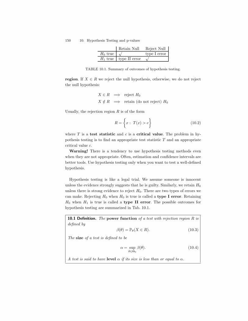
150 10. Hypothesis Testing and p-values
Retain Null Reject NullH0 true
/type I error
H1 true type II error/
TABLE 10.1. Summary of outcomes of hypothesis testing.
region. If X $ R we reject the null hypothesis, otherwise, we do not rejectthe null hypothesis:
X $ R =+ reject H0
X /$ R =+ retain (do not reject) H0
Usually, the rejection region R is of the form
R ='
x : T (x) > c
2(10.2)
where T is a test statistic and c is a critical value. The problem in hy-pothesis testing is to find an appropriate test statistic T and an appropriatecritical value c.
Warning! There is a tendency to use hypothesis testing methods evenwhen they are not appropriate. Often, estimation and confidence intervals arebetter tools. Use hypothesis testing only when you want to test a well-definedhypothesis.
Hypothesis testing is like a legal trial. We assume someone is innocentunless the evidence strongly suggests that he is guilty. Similarly, we retain H0
unless there is strong evidence to reject H0. There are two types of errors wecan make. Rejecting H0 when H0 is true is called a type I error. RetainingH0 when H1 is true is called a type II error. The possible outcomes forhypothesis testing are summarized in Tab. 10.1.
10.1 Definition. The power function of a test with rejection region R isdefined by
((0) = P((X $ R). (10.3)
The size of a test is defined to be
) = sup(#!0
((0). (10.4)
A test is said to have level ) if its size is less than or equal to ).
10. Hypothesis Testing and p-values 151
A hypothesis of the form 0 = 00 is called a simple hypothesis. A hypoth-esis of the form 0 > 00 or 0 < 00 is called a composite hypothesis. A testof the form
H0 : 0 = 00 versus H1 : 0 (= 00
is called a two-sided test. A test of the form
H0 : 0 , 00 versus H1 : 0 > 00
orH0 : 0 * 00 versus H1 : 0 < 00
is called a one-sided test. The most common tests are two-sided.
10.2 Example. Let X1, . . . , Xn ! N(µ,#) where # is known. We want to testH0 : µ , 0 versus H1 : µ > 0. Hence, "0 = ("#, 0] and "1 = (0,#).Consider the test:
reject H0 if T > c
where T = X . The rejection region is
R ='
(x1, . . . , xn) : T (x1, . . . , xn) > c
2.
Let Z denote a standard Normal random variable. The power function is
((µ) = Pµ
;X > c
<
= Pµ
-/n(X " µ)
#>
/n(c" µ)#
.
= P-
Z >
/n(c" µ)#
.
= 1" %-/
n(c" µ)#
..
This function is increasing in µ. See Figure 10.1. Hence
size = supµ%0
((µ) = ((0) = 1" %-/
nc
#
..
For a size ) test, we set this equal to ) and solve for c to get
c =#%$1(1" ))/
n.
We reject when X > #%$1(1" ))//
n. Equivalently, we reject when/
n (X " 0)#
> z#.
where z# = %$1(1 " )). !
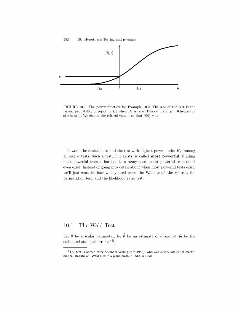
152 10. Hypothesis Testing and p-values
)
µ
((µ)
H0 H1
FIGURE 10.1. The power function for Example 10.2. The size of the test is thelargest probability of rejecting H0 when H0 is true. This occurs at µ = 0 hence thesize is "(0). We choose the critical value c so that "(0) = #.
It would be desirable to find the test with highest power under H1, amongall size ) tests. Such a test, if it exists, is called most powerful. Findingmost powerful tests is hard and, in many cases, most powerful tests don’teven exist. Instead of going into detail about when most powerful tests exist,we’ll just consider four widely used tests: the Wald test,1 the !2 test, thepermutation test, and the likelihood ratio test.
10.1 The Wald Test
Let 0 be a scalar parameter, let 10 be an estimate of 0 and let 1se be theestimated standard error of 10.
1The test is named after Abraham Wald (1902–1950), who was a very influential mathe-matical statistician. Wald died in a plane crash in India in 1950.
10.1 The Wald Test 153
10.3 Definition. The Wald Test
Consider testing
H0 : 0 = 00 versus H1 : 0 (= 00.
Assume that 10 is asymptotically Normal:
(10 " 00)1se
! N(0, 1).
The size ) Wald test is: reject H0 when |W | > z#/2 where
W =10 " 001se
. (10.5)
10.4 Theorem. Asymptotically, the Wald test has size ), that is,
P(0;|W | > z#/2
<) )
as n)#.
Proof. Under 0 = 00, (10 " 00)/1se ! N(0, 1). Hence, the probability ofrejecting when the null 0 = 00 is true is
P(0;|W | > z#/2
<= P(0
(|10 " 00|1se
> z#/2
)
) P;|Z| > z#/2
<
= )
where Z ! N(0, 1). !
10.5 Remark. An alternative version of the Wald test statistic is W = (10 "00)/se0 where se0 is the standard error computed at 0 = 00. Both versions ofthe test are valid.
Let us consider the power of the Wald test when the null hypothesis is false.
10.6 Theorem. Suppose the true value of 0 is 0) (= 00. The power ((0)) — theprobability of correctly rejecting the null hypothesis — is given (approximately)by
1" %-00 " 0)1se
+ z#/2
.+ %
-00 " 0)1se" z#/2
.. (10.6)
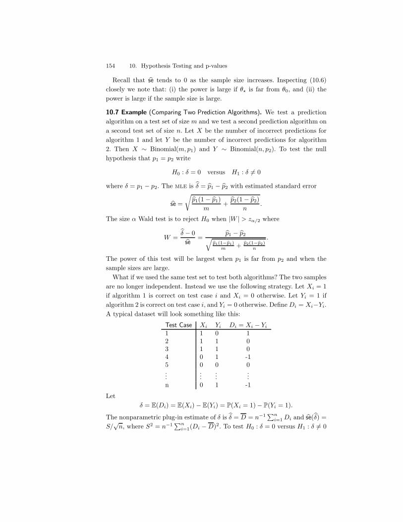
154 10. Hypothesis Testing and p-values
Recall that 1se tends to 0 as the sample size increases. Inspecting (10.6)closely we note that: (i) the power is large if 0) is far from 00, and (ii) thepower is large if the sample size is large.
10.7 Example (Comparing Two Prediction Algorithms). We test a predictionalgorithm on a test set of size m and we test a second prediction algorithm ona second test set of size n. Let X be the number of incorrect predictions foralgorithm 1 and let Y be the number of incorrect predictions for algorithm2. Then X ! Binomial(m, p1) and Y ! Binomial(n, p2). To test the nullhypothesis that p1 = p2 write
H0 : $ = 0 versus H1 : $ (= 0
where $ = p1 " p2. The mle is 1$ = 1p1 " 1p2 with estimated standard error
1se =
U1p1(1" 1p1)
m+1p2(1" 1p2)
n.
The size ) Wald test is to reject H0 when |W | > z#/2 where
W =1$ " 01se
=1p1 " 1p2V
1p1(1$1p1)m + 1p2(1$1p2)
n
.
The power of this test will be largest when p1 is far from p2 and when thesample sizes are large.
What if we used the same test set to test both algorithms? The two samplesare no longer independent. Instead we use the following strategy. Let Xi = 1if algorithm 1 is correct on test case i and Xi = 0 otherwise. Let Yi = 1 ifalgorithm 2 is correct on test case i, and Yi = 0 otherwise. Define Di = Xi"Yi.A typical dataset will look something like this:
Test Case Xi Yi Di = Xi " Yi
1 1 0 12 1 1 03 1 1 04 0 1 -15 0 0 0...
......
...n 0 1 -1
Let$ = E(Di) = E(Xi)" E(Yi) = P(Xi = 1)" P(Yi = 1).
The nonparametric plug-in estimate of $ is 1$ = D = n$10n
i=1 Di and 1se(1$) =S//
n, where S2 = n$10n
i=1(Di "D)2. To test H0 : $ = 0 versus H1 : $ (= 0
10.1 The Wald Test 155
we use W = 1$/1se and reject H0 if |W | > z#/2. This is called a pairedcomparison. !
10.8 Example (Comparing Two Means). Let X1, . . . , Xm and Y1, . . ., Yn betwo independent samples from populations with means µ1 and µ2, respec-tively. Let’s test the null hypothesis that µ1 = µ2. Write this as H0 : $ = 0versus H1 : $ (= 0 where $ = µ1 " µ2. Recall that the nonparametric plug-inestimate of $ is 1$ = X " Y with estimated standard error
1se =
Us21
m+
s22
n
where s21 and s2
2 are the sample variances. The size ) Wald test rejects H0
when |W | > z#/2 where
W =1$ " 01se
=X " YV
s21
m + s22
n
. !
10.9 Example (Comparing Two Medians). Consider the previous example againbut let us test whether the medians of the two distributions are the same.Thus, H0 : $ = 0 versus H1 : $ (= 0 where $ = *1 " *2 where *1 and *2 arethe medians. The nonparametric plug-in estimate of $ is 1$ = 1*1" 1*2 where 1*1and 1*2 are the sample medians. The estimated standard error 1se of 1$ can beobtained from the bootstrap. The Wald test statistic is W = 1$/1se. !
There is a relationship between the Wald test and the 1 " ) asymptoticconfidence interval 10 ± 1se z#/2.
10.10 Theorem. The size ) Wald test rejects H0 : 0 = 00 versus H1 : 0 (= 00if and only if 00 /$ C where
C = (10 " 1se z#/2, 10 + 1se z#/2).
Thus, testing the hypothesis is equivalent to checking whether the null valueis in the confidence interval.
Warning! When we reject H0 we often say that the result is statisticallysignificant. A result might be statistically significant and yet the size of thee!ect might be small. In such a case we have a result that is statistically sig-nificant but not scientifically or practically significant. The di!erence betweenstatistical significance and scientific significance is easy to understand in lightof Theorem 10.10. Any confidence interval that excludes 00 corresponds to re-jecting H0. But the values in the interval could be close to 00 (not scientificallysignificant) or far from 00 (scientifically significant). See Figure 10.2.
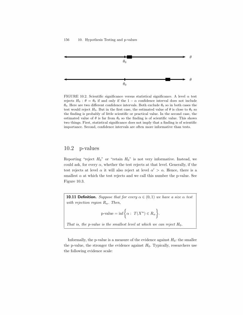
156 10. Hypothesis Testing and p-values
000
000
FIGURE 10.2. Scientific significance versus statistical significance. A level # testrejects H0 : ! = !0 if and only if the 1 % # confidence interval does not include!0. Here are two di"erent confidence intervals. Both exclude !0 so in both cases thetest would reject H0. But in the first case, the estimated value of ! is close to !0 sothe finding is probably of little scientific or practical value. In the second case, theestimated value of ! is far from !0 so the finding is of scientific value. This showstwo things. First, statistical significance does not imply that a finding is of scientificimportance. Second, confidence intervals are often more informative than tests.
10.2 p-values
Reporting “reject H0” or “retain H0” is not very informative. Instead, wecould ask, for every ), whether the test rejects at that level. Generally, if thetest rejects at level ) it will also reject at level )& > ). Hence, there is asmallest ) at which the test rejects and we call this number the p-value. SeeFigure 10.3.
10.11 Definition. Suppose that for every ) $ (0, 1) we have a size ) testwith rejection region R#. Then,
p-value = inf') : T (Xn) $ R#
2.
That is, the p-value is the smallest level at which we can reject H0.
Informally, the p-value is a measure of the evidence against H0: the smallerthe p-value, the stronger the evidence against H0. Typically, researchers usethe following evidence scale:
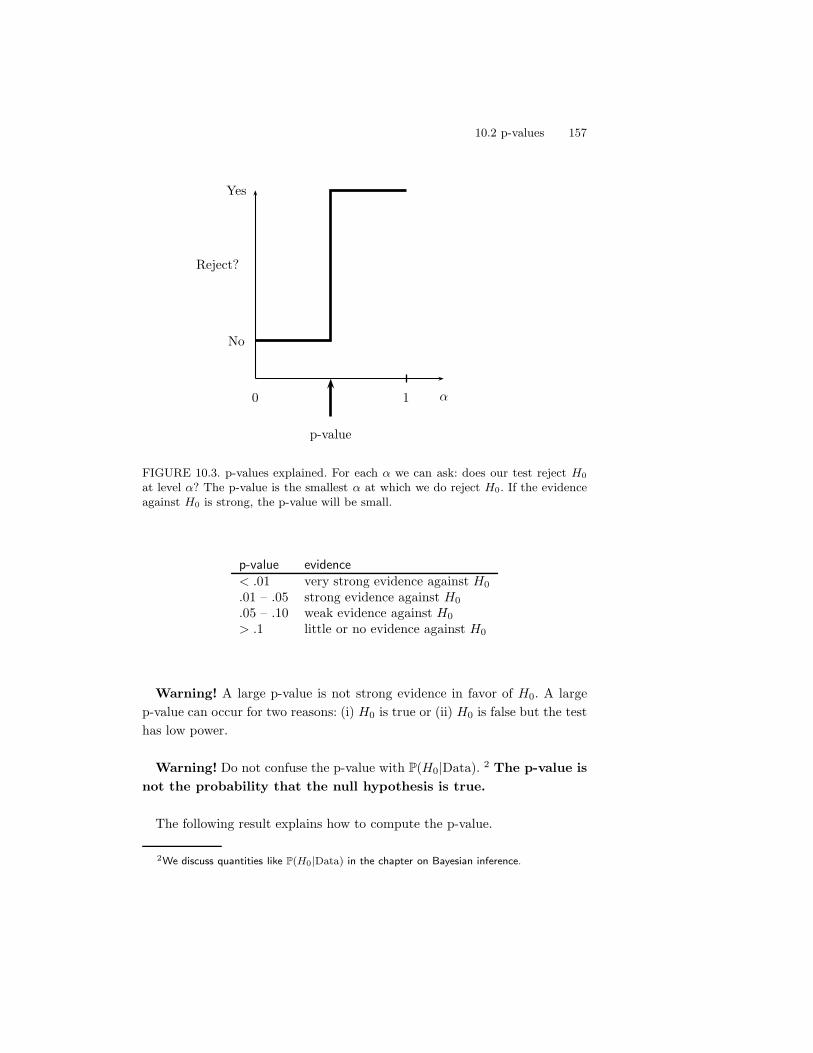
10.2 p-values 157
No
Yes
Reject?
)0 1
p-value
FIGURE 10.3. p-values explained. For each # we can ask: does our test reject H0
at level #? The p-value is the smallest # at which we do reject H0. If the evidenceagainst H0 is strong, the p-value will be small.
p-value evidence< .01 very strong evidence against H0
.01 – .05 strong evidence against H0
.05 – .10 weak evidence against H0
> .1 little or no evidence against H0
Warning! A large p-value is not strong evidence in favor of H0. A largep-value can occur for two reasons: (i) H0 is true or (ii) H0 is false but the testhas low power.
Warning! Do not confuse the p-value with P(H0|Data). 2 The p-value isnot the probability that the null hypothesis is true.
The following result explains how to compute the p-value.
2We discuss quantities like P(H0|Data) in the chapter on Bayesian inference.
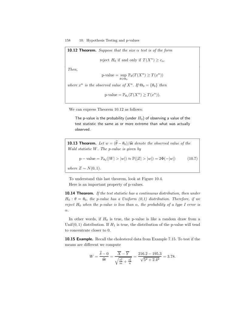
158 10. Hypothesis Testing and p-values
10.12 Theorem. Suppose that the size ) test is of the form
reject H0 if and only if T (Xn) * c#.
Then,p-value = sup
(#!0
P((T (Xn) * T (xn))
where xn is the observed value of Xn. If "0 = {00} then
p-value = P(0(T (Xn) * T (xn)).
We can express Theorem 10.12 as follows:
The p-value is the probability (under H0) of observing a value of the
test statistic the same as or more extreme than what was actually
observed.
10.13 Theorem. Let w = (10 " 00)/1se denote the observed value of theWald statistic W . The p-value is given by
p" value = P(0(|W | > |w|) . P(|Z| > |w|) = 2%("|w|) (10.7)
where Z ! N(0, 1).
To understand this last theorem, look at Figure 10.4.Here is an important property of p-values.
10.14 Theorem. If the test statistic has a continuous distribution, then underH0 : 0 = 00, the p-value has a Uniform (0,1) distribution. Therefore, if wereject H0 when the p-value is less than ), the probability of a type I error is).
In other words, if H0 is true, the p-value is like a random draw from aUnif(0, 1) distribution. If H1 is true, the distribution of the p-value will tendto concentrate closer to 0.
10.15 Example. Recall the cholesterol data from Example 7.15. To test if themeans are di!erent we compute
W =1$ " 01se
=X " YV
s21
m + s22
n
=216.2" 195.3/
52 + 2.42= 3.78.
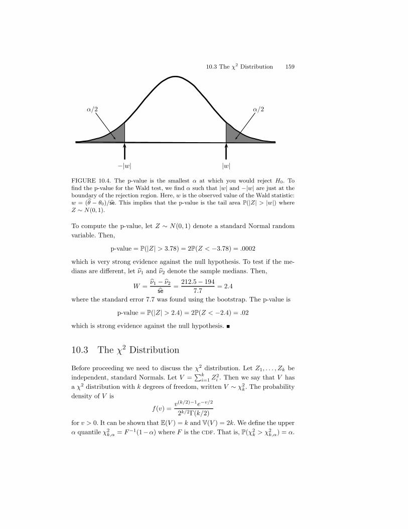
10.3 The $2 Distribution 159
|w|"|w|
)/2)/2
FIGURE 10.4. The p-value is the smallest # at which you would reject H0. Tofind the p-value for the Wald test, we find # such that |w| and %|w| are just at theboundary of the rejection region. Here, w is the observed value of the Wald statistic:w = (1! % !0)/1se. This implies that the p-value is the tail area P(|Z| > |w|) whereZ & N(0, 1).
To compute the p-value, let Z ! N(0, 1) denote a standard Normal randomvariable. Then,
p-value = P(|Z| > 3.78) = 2P(Z < "3.78) = .0002
which is very strong evidence against the null hypothesis. To test if the me-dians are di!erent, let 1*1 and 1*2 denote the sample medians. Then,
W =1*1 " 1*21se
=212.5" 194
7.7= 2.4
where the standard error 7.7 was found using the bootstrap. The p-value is
p-value = P(|Z| > 2.4) = 2P(Z < "2.4) = .02
which is strong evidence against the null hypothesis. !
10.3 The !2 Distribution
Before proceeding we need to discuss the !2 distribution. Let Z1, . . . , Zk beindependent, standard Normals. Let V =
0ki=1 Z2
i . Then we say that V hasa !2 distribution with k degrees of freedom, written V ! !2
k. The probabilitydensity of V is
f(v) =v(k/2)$1e$v/2
2k/2&(k/2)for v > 0. It can be shown that E(V ) = k and V(V ) = 2k. We define the upper) quantile !2
k,# = F$1(1")) where F is the cdf. That is, P(!2k > !2
k,#) = ).
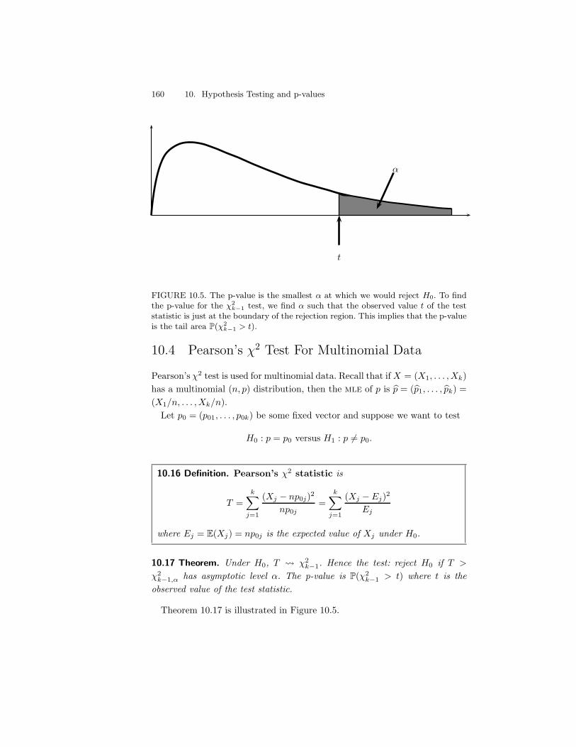
160 10. Hypothesis Testing and p-values
t
)
FIGURE 10.5. The p-value is the smallest # at which we would reject H0. To findthe p-value for the $2
k!1 test, we find # such that the observed value t of the teststatistic is just at the boundary of the rejection region. This implies that the p-valueis the tail area P($2
k!1 > t).
10.4 Pearson’s !2 Test For Multinomial Data
Pearson’s !2 test is used for multinomial data. Recall that if X = (X1, . . . , Xk)has a multinomial (n, p) distribution, then the mle of p is 1p = (1p1, . . . , 1pk) =(X1/n, . . . , Xk/n).
Let p0 = (p01, . . . , p0k) be some fixed vector and suppose we want to test
H0 : p = p0 versus H1 : p (= p0.
10.16 Definition. Pearson’s !2 statistic is
T =k*
j=1
(Xj " np0j)2
np0j=
k*
j=1
(Xj " Ej)2
Ej
where Ej = E(Xj) = np0j is the expected value of Xj under H0.
10.17 Theorem. Under H0, T ! !2k$1. Hence the test: reject H0 if T >
!2k$1,# has asymptotic level ). The p-value is P(!2
k$1 > t) where t is theobserved value of the test statistic.
Theorem 10.17 is illustrated in Figure 10.5.
10.5 The Permutation Test 161
10.18 Example (Mendel’s peas). Mendel bred peas with round yellow seedsand wrinkled green seeds. There are four types of progeny: round yellow,wrinkled yellow, round green, and wrinkled green. The number of each typeis multinomial with probability p = (p1, p2, p3, p4). His theory of inheritancepredicts that p is equal to
p0 0-
916
,316
,316
,116
..
In n = 556 trials he observed X = (315, 101, 108, 32). We will test H0 : p = p0
versus H1 : p (= p0. Since, np01 = 312.75, np02 = np03 = 104.25, and np04 =34.75, the test statistic is
!2 =(315" 312.75)2
312.75+
(101" 104.25)2
104.25
+(108" 104.25)2
104.25+
(32" 34.75)2
34.75= 0.47.
The ) = .05 value for a !23 is 7.815. Since 0.47 is not larger than 7.815 we do
not reject the null. The p-value is
p-value = P(!23 > .47) = .93
which is not evidence against H0. Hence, the data do not contradict Mendel’stheory.3!
In the previous example, one could argue that hypothesis testing is not theright tool. Hypothesis testing is useful to see if there is evidence to reject H0.This is appropriate when H0 corresponds to the status quo. It is not useful forproving that H0 is true. Failure to reject H0 might occur because H0 is true,but it might occur just because the test has low power. Perhaps a confidenceset for the distance between p and p0 might be more useful in this example.
10.5 The Permutation Test
The permutation test is a nonparametric method for testing whether twodistributions are the same. This test is “exact,” meaning that it is not basedon large sample theory approximations. Suppose that X1, . . ., Xm ! FX andY1, . . ., Yn ! FY are two independent samples and H0 is the hypothesis that
3There is some controversy about whether Mendel’s results are “too good.”
162 10. Hypothesis Testing and p-values
the two samples are identically distributed. This is the type of hypothesis wewould consider when testing whether a treatment di!ers from a placebo. Moreprecisely we are testing
H0 : FX = FY versus H1 : FX (= FY .
Let T (x1, . . . , xm, y1, . . . , yn) be some test statistic, for example,
T (X1, . . . , Xm, Y1, . . . , Yn) = |Xm " Y n|.
Let N = m+n and consider forming all N ! permutations of the data X1, . . .,Xm, Y1, . . ., Yn. For each permutation, compute the test statistic T . Denotethese values by T1, . . . , TN !. Under the null hypothesis, each of these values isequally likely. 4 The distribution P0 that puts mass 1/N ! on each Tj is calledthe permutation distribution of T . Let tobs be the observed value of thetest statistic. Assuming we reject when T is large, the p-value is
p-value = P0(T > tobs) =1
N !
N !*
j=1
I(Tj > tobs).
10.19 Example. Here is a toy example to make the idea clear. Suppose thedata are: (X1, X2, Y1) = (1, 9, 3). Let T (X1, X2, Y1) = |X " Y | = 2. Thepermutations are:
permutation value of T probability(1,9,3) 2 1/6(9,1,3) 2 1/6(1,3,9) 7 1/6(3,1,9) 7 1/6(3,9,1) 5 1/6(9,3,1) 5 1/6
The p-value is P(T > 2) = 4/6. !
Usually, it is not practical to evaluate all N ! permutations. We can approx-imate the p-value by sampling randomly from the set of permutations. Thefraction of times Tj > tobs among these samples approximates the p-value.
4More precisely, under the null hypothesis, given the ordered data values,X1, . . . , Xm, Y1, . . . , Yn is uniformly distributed over the N ! permutations of the data.
10.5 The Permutation Test 163
Algorithm for Permutation Test
1. Compute the observed value of the test statistictobs = T (X1, . . . , Xm, Y1, . . . , Yn).
2. Randomly permute the data. Compute the statistic again using thepermuted data.
3. Repeat the previous step B times and let T1, . . . , TB denote theresulting values.
4. The approximate p-value is
1B
B*
j=1
I(Tj > tobs).
10.20 Example. DNA microarrays allow researchers to measure the expres-sion levels of thousands of genes. The data are the levels of messenger RNA(mRNA) of each gene, which is thought to provide a measure of how muchprotein that gene produces. Roughly, the larger the number, the more activethe gene. The table below, reproduced from Efron et al. (2001) shows theexpression levels for genes from ten patients with two types of liver cancercells. There are 2,638 genes in this experiment but here we show just the firsttwo. The data are log-ratios of the intensity levels of two di!erent color dyesused on the arrays.
Type I Type IIPatient 1 2 3 4 5 6 7 8 9 10Gene 1 230 -1,350 -1,580 -400 -760 970 110 -50 -190 -200Gene 2 470 -850 -.8 -280 120 390 -1730 -1360 -1 -330...
......
......
......
......
......
Let’s test whether the median level of gene 1 is di!erent between the twogroups. Let *1 denote the median level of gene 1 of Type I and let *2 denote themedian level of gene 1 of Type II. The absolute di!erence of sample mediansis T = |1*1 " 1*2| = 710. Now we estimate the permutation distribution bysimulation and we find that the estimated p-value is .045. Thus, if we use a) = .05 level of significance, we would say that there is evidence to reject thenull hypothesis of no di!erence. !
164 10. Hypothesis Testing and p-values
In large samples, the permutation test usually gives similar results to a testthat is based on large sample theory. The permutation test is thus most usefulfor small samples.
10.6 The Likelihood Ratio Test
The Wald test is useful for testing a scalar parameter. The likelihood ratiotest is more general and can be used for testing a vector-valued parameter.
10.21 Definition. Consider testing
H0 : 0 $ "0 versus H1 : 0 /$ "0.
The likelihood ratio statistic is
% = 2 log-
sup(#! L(0)sup(#!0
L(0)
.= 2 log
(L(10)L(100)
)
where 10 is the mle and 100 is the mle when 0 is restricted to lie in "0.
You might have expected to see the maximum of the likelihood over "c0
instead of " in the numerator. In practice, replacing "c0 with " has little
e!ect on the test statistic. Moreover, the theoretical properties of % are muchsimpler if the test statistic is defined this way.
The likelihood ratio test is most useful when "0 consists of all parametervalues 0 such that some coordinates of 0 are fixed at particular values.
10.22 Theorem. Suppose that 0 = (01, . . . , 0q, 0q+1, . . . , 0r). Let
"0 = {0 : (0q+1, . . . , 0r) = (00,q+1, . . . , 00,r)}.
Let % be the likelihood ratio test statistic. Under H0 : 0 $ "0,
%(xn) ! !2r$q
where r " q is the dimension of " minus the dimension of "0. The p-valuefor the test is P(!2
r$q > %).
For example, if 0 = (01, 02, 03, 04, 05) and we want to test the null hypothesisthat 04 = 05 = 0 then the limiting distribution has 5 " 3 = 2 degrees offreedom.
10.7 Multiple Testing 165
10.23 Example (Mendel’s Peas Revisited). Consider example 10.18 again. Thelikelihood ratio test statistic for H0 : p = p0 versus H1 : p (= p0 is
% = 2 log-
L(1p)L(p0)
.
= 24*
j=1
Xj log-1pj
p0j
.
= 2-
315 log- 315
556916
.+ 101 log
- 101556316
.
+108 log- 108
556316
.+ 32 log
- 32556116
..
= 0.48.
Under H1 there are four parameters. However, the parameters must sum toone so the dimension of the parameter space is three. Under H0 there are nofree parameters so the dimension of the restricted parameter space is zero. Thedi!erence of these two dimensions is three. Therefore, the limiting distributionof % under H0 is !2
3 and the p-value is
p-value = P(!23 > .48) = .92.
The conclusion is the same as with the !2 test. !
When the likelihood ratio test and the !2 test are both applicable, as in thelast example, they usually lead to similar results as long as the sample size islarge.
10.7 Multiple Testing
In some situations we may conduct many hypothesis tests. In example 10.20,there were actually 2,638 genes. If we tested for a di!erence for each gene,we would be conducting 2,638 separate hypothesis tests. Suppose each testis conducted at level ). For any one test, the chance of a false rejection ofthe null is ). But the chance of at least one false rejection is much higher.This is the multiple testing problem. The problem comes up in many datamining situations where one may end up testing thousands or even millions ofhypotheses. There are many ways to deal with this problem. Here we discusstwo methods.

166 10. Hypothesis Testing and p-values
Consider m hypothesis tests:
H0i versus H1i, i = 1, . . . , m
and let P1, . . . , Pm denote the m p-values for these tests.
The Bonferroni Method
Given p-values P1, . . . , Pm, reject null hypothesis H0i if
Pi <)
m.
10.24 Theorem. Using the Bonferroni method, the probability of falsely re-jecting any null hypotheses is less than or equal to ).
Proof. Let R be the event that at least one null hypothesis is falselyrejected. Let Ri be the event that the ith null hypothesis is falsely rejected.Recall that if A1, . . . , Ak are events then P(
&ki=1 Ai) ,
0ki=1 P(Ai). Hence,
P(R) = P(
m#
i=1
Ri
),
m*
i=1
P(Ri) =m*
i=1
)
m= )
from Theorem 10.14. !
10.25 Example. In the gene example, using ) = .05, we have that .05/2, 638 =.00001895375. Hence, for any gene with p-value less than .00001895375, wedeclare that there is a significant di!erence. !
The Bonferroni method is very conservative because it is trying to makeit unlikely that you would make even one false rejection. Sometimes, a morereasonable idea is to control the false discovery rate (FDR) which is de-fined as the mean of the number of false rejections divided by the number ofrejections.
Suppose we reject all null hypotheses whose p-values fall below some thresh-old. Let m0 be the number of null hypotheses that are true and let m1 =m"m0. The tests can be categorized in a 2- 2 as in Table 10.2.
Define the False Discovery Proportion (FDP)
FDP ='
V/R if R > 00 if R = 0.
The FDP is the proportion of rejections that are incorrect. Next define FDR =E(FDP).
10.7 Multiple Testing 167
H0 Not Rejected H0 Rejected TotalH0 True U V m0
H0 False T S m1
Total m"R R m
TABLE 10.2. Types of outcomes in multiple testing.
The Benjamini-Hochberg (BH) Method
1. Let P(1) < · · · < P(m) denote the ordered p-values.
2. Define
4i =i)
Cmm, and R = max
'i : P(i) < 4i
2(10.8)
where Cm is defined to be 1 if the p-values are independent andCm =
0mi=1(1/i) otherwise.
3. Let T = P(R); we call T the BH rejection threshold.
4. Reject all null hypotheses H0i for which Pi , T.
10.26 Theorem (Benjamini and Hochberg). If the procedure above is applied,then regardless of how many nulls are true and regardless of the distributionof the p-values when the null hypothesis is false,
FDR = E(FDP) , m0
m) , ).
10.27 Example. Figure 10.6 shows six ordered p-values plotted as verticallines. If we tested at level ) without doing any correction for multiple testing,we would reject all hypotheses whose p-values are less than ). In this case,the four hypotheses corresponding to the four smallest p-values are rejected.The Bonferroni method rejects all hypotheses whose p-values are less than)/m. In this case, this leads to no rejections. The BH threshold correspondsto the last p-value that falls under the line with slope ). This leads to twohypotheses being rejected in this case. !
10.28 Example. Suppose that 10 independent hypothesis tests are carriedleading to the following ordered p-values:
0.00017 0.00448 0.00671 0.00907 0.01220
0.33626 0.39341 0.53882 0.58125 0.98617
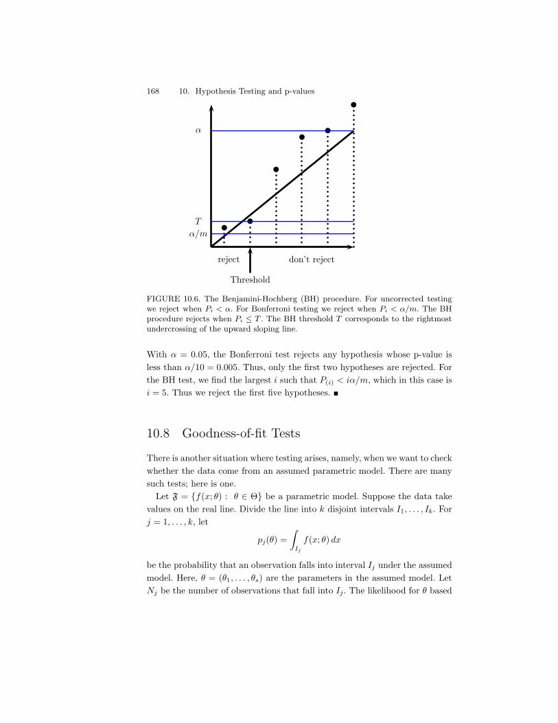
168 10. Hypothesis Testing and p-values
Threshold
reject don’t reject
)
T
)/m
FIGURE 10.6. The Benjamini-Hochberg (BH) procedure. For uncorrected testingwe reject when Pi < #. For Bonferroni testing we reject when Pi < #/m. The BHprocedure rejects when Pi " T . The BH threshold T corresponds to the rightmostundercrossing of the upward sloping line.
With ) = 0.05, the Bonferroni test rejects any hypothesis whose p-value isless than )/10 = 0.005. Thus, only the first two hypotheses are rejected. Forthe BH test, we find the largest i such that P(i) < i)/m, which in this case isi = 5. Thus we reject the first five hypotheses. !
10.8 Goodness-of-fit Tests
There is another situation where testing arises, namely, when we want to checkwhether the data come from an assumed parametric model. There are manysuch tests; here is one.
Let F = {f(x; 0) : 0 $ "} be a parametric model. Suppose the data takevalues on the real line. Divide the line into k disjoint intervals I1, . . . , Ik. Forj = 1, . . . , k, let
pj(0) =9
Ij
f(x; 0) dx
be the probability that an observation falls into interval Ij under the assumedmodel. Here, 0 = (01, . . . , 0s) are the parameters in the assumed model. LetNj be the number of observations that fall into Ij . The likelihood for 0 based
10.9 Bibliographic Remarks 169
on the counts N1, . . . , Nk is the multinomial likelihood
Q(0) =k/
j=1
pi(0)Nj .
Maximizing Q(0) yields estimates c0 = (c01, . . . , c0s) of 0. Now define the teststatistic
Q =k*
j=1
(Nj " npj(c0))2
npj(c0). (10.9)
10.29 Theorem. Let H0 be the null hypothesis that the data are iiddraws fromthe model F = {f(x; 0) : 0 $ "}. Under H " 0, the statistic Q defined inequation (10.9) converges in distribution to a !2
k$1$s random variable. Thus,the (approximate) p-value for the test is P(!2
k$1$s > q) where q denotes theobserved value of Q.
It is tempting to replace c0 in (10.9) with the mle 10. However, this will notresult in a statistic whose limiting distribution is a !2
k$1$s. However, it canbe shown — due to a theorem of Herman Cherno! and Erich Lehmann from1954 — that the p-value is bounded approximately by the p-values obtainedusing a !2
k$1$s and a !2k$1.
Goodness-of-fit testing has some serious limitations. If reject H0 then weconclude we should not use the model. But if we do not reject H0 we can-not conclude that the model is correct. We may have failed to reject simplybecause the test did not have enough power. This is why it is better to usenonparametric methods whenever possible rather than relying on parametricassumptions.
10.9 Bibliographic Remarks
The most complete book on testing is Lehmann (1986). See also Chapter 8 ofCasella and Berger (2002) and Chapter 9 of Rice (1995). The FDR method isdue to Benjamini and Hochberg (1995). Some of the exercises are from Rice(1995).
170 10. Hypothesis Testing and p-values
10.10 Appendix
10.10.1 The Neyman-Pearson Lemma
In the special case of a simple null H0 : 0 = 00 and a simple alternativeH1 : 0 = 01 we can say precisely what the most powerful test is.
10.30 Theorem (Neyman-Pearson). Suppose we test H0 : 0 = 00 versus H1 :0 = 01. Let
T =L(01)L(00)
=Dn
i=1 f(xi; 01)Dni=1 f(xi; 00)
.
Suppose we reject H0 when T > k. If we choose k so that P(0(T > k) = )
then this test is the most powerful, size ) test. That is, among all tests withsize ), this test maximizes the power ((01).
10.10.2 The t-test
To test H0 : µ = µ0 where µ = E(Xi) is the mean, we can use the Wald test.When the data are assumed to be Normal and the sample size is small, it iscommon instead to use the t-test. A random variable T has a t-distributionwith k degrees of freedom if it has density
f(t) =&;
k+12
<
/k&&
;k2
< ;1 + t2
k
<(k+1)/2.
When the degrees of freedom k ) #, this tends to a Normal distribution.When k = 1 it reduces to a Cauchy.
Let X1, . . . , Xn ! N(µ,#2) where 0 = (µ,#2) are both unknown. Supposewe want to test µ = µ0 versus µ (= µ0. Let
T =/
n(Xn " µ0)Sn
where S2n is the sample variance. For large samples T . N(0, 1) under H0.
The exact distribution of T under H0 is tn$1. Hence if we reject when |T | >
tn$1,#/2 then we get a size ) test. However, when n is moderately large, thet-test is essentially identical to the Wald test.
10.11 Exercises
1. Prove Theorem 10.6.

10.11 Exercises 171
2. Prove Theorem 10.14.
3. Prove Theorem 10.10.
4. Prove Theorem 10.12.
5. Let X1, ..., Xn ! Uniform(0, 0) and let Y = max{X1, ..., Xn}. We wantto test
H0 : 0 = 1/2 versus H1 : 0 > 1/2.
The Wald test is not appropriate since Y does not converge to a Normal.Suppose we decide to test this hypothesis by rejecting H0 when Y > c.
(a) Find the power function.
(b) What choice of c will make the size of the test .05?
(c) In a sample of size n = 20 with Y=0.48 what is the p-value? Whatconclusion about H0 would you make?
(d) In a sample of size n = 20 with Y=0.52 what is the p-value? Whatconclusion about H0 would you make?
6. There is a theory that people can postpone their death until after animportant event. To test the theory, Phillips and King (1988) collecteddata on deaths around the Jewish holiday Passover. Of 1919 deaths, 922died the week before the holiday and 997 died the week after. Think ofthis as a binomial and test the null hypothesis that 0 = 1/2. Report andinterpret the p-value. Also construct a confidence interval for 0.
7. In 1861, 10 essays appeared in the New Orleans Daily Crescent. Theywere signed “Quintus Curtius Snodgrass” and some people suspectedthey were actually written by Mark Twain. To investigate this, we willconsider the proportion of three letter words found in an author’s work.From eight Twain essays we have:
.225 .262 .217 .240 .230 .229 .235 .217
From 10 Snodgrass essays we have:
.209 .205 .196 .210 .202 .207 .224 .223 .220 .201
(a) Perform a Wald test for equality of the means. Use the nonparamet-ric plug-in estimator. Report the p-value and a 95 per cent confidenceinterval for the di!erence of means. What do you conclude?
(b) Now use a permutation test to avoid the use of large sample methods.What is your conclusion? (Brinegar (1963)).
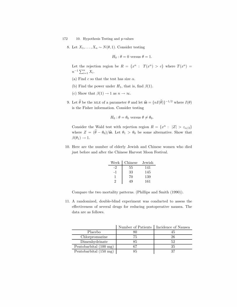
172 10. Hypothesis Testing and p-values
8. Let X1, . . . , Xn ! N(0, 1). Consider testing
H0 : 0 = 0 versus 0 = 1.
Let the rejection region be R = {xn : T (xn) > c} where T (xn) =n$1
0ni=1 Xi.
(a) Find c so that the test has size ).
(b) Find the power under H1, that is, find ((1).
(c) Show that ((1)) 1 as n)#.
9. Let 10 be the mle of a parameter 0 and let 1se = {nI(10)}$1/2 where I(0)is the Fisher information. Consider testing
H0 : 0 = 00 versus 0 (= 00.
Consider the Wald test with rejection region R = {xn : |Z| > z#/2}where Z = (10 " 00)/1se. Let 01 > 00 be some alternative. Show that((01)) 1.
10. Here are the number of elderly Jewish and Chinese women who diedjust before and after the Chinese Harvest Moon Festival.
Week Chinese Jewish-2 55 141-1 33 1451 70 1392 49 161
Compare the two mortality patterns. (Phillips and Smith (1990)).
11. A randomized, double-blind experiment was conducted to assess thee!ectiveness of several drugs for reducing postoperative nausea. Thedata are as follows.
Number of Patients Incidence of NauseaPlacebo 80 45
Chlorpromazine 75 26Dimenhydrinate 85 52
Pentobarbital (100 mg) 67 35Pentobarbital (150 mg) 85 37
10.11 Exercises 173
(a) Test each drug versus the placebo at the 5 per cent level. Also, reportthe estimated odds–ratios. Summarize your findings.
(b) Use the Bonferroni and the FDR method to adjust for multipletesting. (Beecher (1959)).
12. Let X1, ..., Xn ! Poisson(%).
(a) Let %0 > 0. Find the size ) Wald test for
H0 : % = %0 versus H1 : % (= %0.
(b) (Computer Experiment.) Let %0 = 1, n = 20 and ) = .05. SimulateX1, . . . , Xn ! Poisson(%0) and perform the Wald test. Repeat manytimes and count how often you reject the null. How close is the type Ierror rate to .05?
13. Let X1, . . . , Xn ! N(µ,#2). Construct the likelihood ratio test for
H0 : µ = µ0 versus H1 : µ (= µ0.
Compare to the Wald test.
14. Let X1, . . . , Xn ! N(µ,#2). Construct the likelihood ratio test for
H0 : # = #0 versus H1 : # (= #0.
Compare to the Wald test.
15. Let X ! Binomial(n, p). Construct the likelihood ratio test for
H0 : p = p0 versus H1 : p (= p0.
Compare to the Wald test.
16. Let 0 be a scalar parameter and suppose we test
H0 : 0 = 00 versus H1 : 0 (= 00.
Let W be the Wald test statistic and let % be the likelihood ratio teststatistic. Show that these tests are equivalent in the sense that
W 2
%P") 1
as n ) #. Hint: Use a Taylor expansion of the log-likelihood 4(0) toshow that
% .-/
n(10 " 00).2-" 1
n4&&(10)
..

This is page 174Printer: Opaque this
This is page 175Printer: Opaque this
11Bayesian Inference
11.1 The Bayesian Philosophy
The statistical methods that we have discussed so far are known as frequen-tist (or classical) methods. The frequentist point of view is based on thefollowing postulates:
F1 Probability refers to limiting relative frequencies. Probabilities are ob-jective properties of the real world.
F2 Parameters are fixed, unknown constants. Because they are not fluctu-ating, no useful probability statements can be made about parameters.
F3 Statistical procedures should be designed to have well-defined long runfrequency properties. For example, a 95 percent confidence interval shouldtrap the true value of the parameter with limiting frequency at least 95percent.
There is another approach to inference called Bayesian inference. TheBayesian approach is based on the following postulates:
176 11. Bayesian Inference
B1 Probability describes degree of belief, not limiting frequency. As such,we can make probability statements about lots of things, not just datawhich are subject to random variation. For example, I might say that“the probability that Albert Einstein drank a cup of tea on August 1,1948” is .35. This does not refer to any limiting frequency. It reflects mystrength of belief that the proposition is true.
B2 We can make probability statements about parameters, even thoughthey are fixed constants.
B3 We make inferences about a parameter 0 by producing a probabilitydistribution for 0. Inferences, such as point estimates and interval esti-mates, may then be extracted from this distribution.
Bayesian inference is a controversial approach because it inherently em-braces a subjective notion of probability. In general, Bayesian methods pro-vide no guarantees on long run performance. The field of statistics puts moreemphasis on frequentist methods although Bayesian methods certainly havea presence. Certain data mining and machine learning communities seem toembrace Bayesian methods very strongly. Let’s put aside philosophical ar-guments for now and see how Bayesian inference is done. We’ll conclude thischapter with some discussion on the strengths and weaknesses of the Bayesianapproach.
11.2 The Bayesian Method
Bayesian inference is usually carried out in the following way.
1. We choose a probability density f(0) — called the prior distribution— that expresses our beliefs about a parameter 0 before we see anydata.
2. We choose a statistical model f(x|0) that reflects our beliefs about x
given 0. Notice that we now write this as f(x|0) instead of f(x; 0).
3. After observing data X1, . . . , Xn, we update our beliefs and calculatethe posterior distribution f(0|X1, . . . , Xn).
To see how the third step is carried out, first suppose that 0 is discrete andthat there is a single, discrete observation X . We should use a capital letter
11.2 The Bayesian Method 177
now to denote the parameter since we are treating it like a random variable,so let " denote the parameter. Now, in this discrete setting,
P(" = 0|X = x) =P(X = x," = 0)
P(X = x)
=P(X = x|" = 0)P(" = 0)0( P(X = x|" = 0)P(" = 0)
which you may recognize from Chapter 1 as Bayes’ theorem. The versionfor continuous variables is obtained by using density functions:
f(0|x) =f(x|0)f(0)8f(x|0)f(0)d0
. (11.1)
If we have n iid observations X1, . . . , Xn, we replace f(x|0) with
f(x1, . . . , xn|0) =n/
i=1
f(xi|0) = Ln(0).
Notation. We will write Xn to mean (X1, . . . , Xn) and xn to mean (x1, . . . , xn).Now,
f(0|xn) =f(xn|0)f(0)8f(xn|0)f(0)d0
=Ln(0)f(0)
cn3 Ln(0)f(0) (11.2)
wherecn =
9Ln(0)f(0)d0 (11.3)
is called the normalizing constant. Note that cn does not depend on 0. Wecan summarize by writing:
Posterior is proportional to Likelihood times Prior
or, in symbols,f(0|xn) 3 L(0)f(0).
You might wonder, doesn’t it cause a problem to throw away the constantcn? The answer is that we can always recover the constant later if we need to.
What do we do with the posterior distribution? First, we can get a pointestimate by summarizing the center of the posterior. Typically, we use themean or mode of the posterior. The posterior mean is
0n =90f(0|xn)d0 =
80Ln(0)f(0)8Ln(0)f(0)d0
. (11.4)
178 11. Bayesian Inference
We can also obtain a Bayesian interval estimate. We find a and b such that8 a$! f(0|xn)d0 =
8!b f(0|xn)d0 = )/2. Let C = (a, b). Then
P(0 $ C|xn) =9 b
af(0|xn) d0 = 1" )
so C is a 1" ) posterior interval.
11.1 Example. Let X1, . . . , Xn ! Bernoulli(p). Suppose we take the uniformdistribution f(p) = 1 as a prior. By Bayes’ theorem, the posterior has theform
f(p|xn) 3 f(p)Ln(p) = ps(1 " p)n$s = ps+1$1(1" p)n$s+1$1
where s =0n
i=1 xi is the number of successes. Recall that a random variablehas a Beta distribution with parameters ) and ( if its density is
f(p; ),() =&()+ ()&())&(()
p#$1(1" p)"$1.
We see that the posterior for p is a Beta distribution with parameters s + 1and n" s + 1. That is,
f(p|xn) =&(n + 2)
&(s + 1)&(n" s + 1)p(s+1)$1(1" p)(n$s+1)$1.
We write this asp|xn ! Beta(s + 1, n" s + 1).
Notice that we have figured out the normalizing constant without actuallydoing the integral
8Ln(p)f(p)dp. The mean of a Beta(),() distribution is
)/()+ () so the Bayes estimator is
p =s + 1n + 2
. (11.5)
It is instructive to rewrite the estimator as
p = %n1p + (1" %n)cp (11.6)
where 1p = s/n is the mle, cp = 1/2 is the prior mean and %n = n/(n + 2) . 1.A 95 percent posterior interval can be obtained by numerically finding a andb such that
8 ba f(p|xn) dp = .95.
Suppose that instead of a uniform prior, we use the prior p ! Beta(),().If you repeat the calculations above, you will see that p|xn ! Beta()+ s,( +
11.2 The Bayesian Method 179
n " s). The flat prior is just the special case with ) = ( = 1. The posteriormean is
p =)+ s
)+ ( + n=-
n
)+ ( + n
.1p +-
)+ (
)+ ( + n
.p0
where p0 = )/()+ () is the prior mean. !
In the previous example, the prior was a Beta distribution and the posteriorwas a Beta distribution. When the prior and the posterior are in the samefamily, we say that the prior is conjugate with respect to the model.
11.2 Example. Let X1, . . . , Xn ! N(0,#2). For simplicity, let us assume that# is known. Suppose we take as a prior 0 ! N(a, b2). In problem 1 in theexercises it is shown that the posterior for 0 is
0|Xn ! N(0, 22) (11.7)
where0 = wX + (1 " w)a,
w =1
se2
1se2 + 1
b2,
122
=1
se2+
1b2
,
and se = #//
n is the standard error of the mle X . This is another exampleof a conjugate prior. Note that w ) 1 and 2/se) 1 as n)#. So, for largen, the posterior is approximately N(10, se2). The same is true if n is fixed butb)#, which corresponds to letting the prior become very flat.
Continuing with this example, let us find C = (c, d) such that P(0 $C|Xn) = .95. We can do this by choosing c and d such that P(0 < c|Xn) =.025 and P(0 > d|Xn) = .025. So, we want to find c such that
P(0 < c|Xn) = P(0 " 02
<c" 02
CCCCC Xn
)
= P-
Z <c" 02
.= .025.
We know that P(Z < "1.96) = .025. So,
c" 02
= "1.96
implying that c = 0"1.962. By similar arguments, d = 0+1.96. So a 95 percentBayesian interval is 0±1.96 2 . Since 0 . 10 and 2 . se, the 95 percent Bayesianinterval is approximated by 10 ± 1.96 se which is the frequentist confidenceinterval. !
180 11. Bayesian Inference
11.3 Functions of Parameters
How do we make inferences about a function 2 = g(0)? Remember in Chapter3 we solved the following problem: given the density fX for X , find the densityfor Y = g(X). We now simply apply the same reasoning. The posterior cdf
for 2 isH(2 |xn) = P(g(0) , 2 |xn) =
9
Af(0|xn)d0
where A = {0 : g(0) , 2}. The posterior density is h(2 |xn) = H &(2 |xn).
11.3 Example. Let X1, . . . , Xn ! Bernoulli(p) and f(p) = 1 so that p|Xn !Beta(s + 1, n" s + 1) with s =
0ni=1 xi. Let , = log(p/(1" p)). Then
H(,|xn) = P(( , ,|xn) = P(
log-
P
1" P
., ,
CCCCC xn
)
= P(
P , e+
1 + e+
CCCCC xn
)
=9 e#/(1+e#)
0f(p|xn) dp
=&(n + 2)
&(s + 1)&(n" s + 1)
9 e#/(1+e#)
0ps(1" p)n$s dp
and
h(,|xn) = H &(,|xn)
=&(n + 2)
&(s + 1)&(n" s + 1)
-e+
1 + e+
.s - 11 + e+
.n$sE
G3+
e#
1+e#
,
3,
H
J
=&(n + 2)
&(s + 1)&(n" s + 1)
-e+
1 + e+
.s - 11 + e+
.n$s- 11 + e+
.2
=&(n + 2)
&(s + 1)&(n" s + 1)
-e+
1 + e+
.s - 11 + e+
.n$s+2
for , $ R. !
11.4 Simulation
The posterior can often be approximated by simulation. Suppose we draw01, . . . , 0B ! p(0|xn). Then a histogram of 01, . . . , 0B approximates the poste-rior density p(0|xn). An approximation to the posterior mean 0n = E(0|xn) is
11.5 Large Sample Properties of Bayes’ Procedures 181
B$10B
j=1 0j . The posterior 1") interval can be approximated by (0#/2, 01$#/2)where 0#/2 is the )/2 sample quantile of 01, . . . , 0B.
Once we have a sample 01, . . . , 0B from f(0|xn), let 2i = g(0i). Then21, . . . , 2B is a sample from f(2 |xn). This avoids the need to do any analyticalcalculations. Simulation is discussed in more detail in Chapter 24.
11.4 Example. Consider again Example 11.3. We can approximate the pos-terior for , without doing any calculus. Here are the steps:
1. Draw P1, . . . , PB ! Beta(s + 1, n" s + 1).
2. Let ,i = log(Pi/(1" Pi)) for i = 1, . . . , B.
Now ,1, . . . ,,B are iid draws from h(,|xn). A histogram of these valuesprovides an estimate of h(,|xn). !
11.5 Large Sample Properties of Bayes’ Procedures
In the Bernoulli and Normal examples we saw that the posterior mean wasclose to the mle. This is true in greater generality.
11.5 Theorem. Let 10n be the mle and let 1se = 1/V
nI(10n). Under appropriateregularity conditions, the posterior is approximately Normal with mean 10n andstandard deviation 1se. Hence, 0n . 10n. Also, if Cn = (10n"z#/2 1se, 10n +z#/2 1se)is the asymptotic frequentist 1 " ) confidence interval, then Cn is also anapproximate 1" ) Bayesian posterior interval:
P(0 $ Cn|Xn)) 1" ).
There is also a Bayesian delta method. Let 2 = g(0). Then
2 |Xn . N(12 , cse2)
where 12 = g(10) and cse = 1se |g&(10)|.
11.6 Flat Priors, Improper Priors, and“Noninformative” Priors
An important question in Bayesian inference is: where does one get the priorf(0)? One school of thought, called subjectivism says that the prior should
182 11. Bayesian Inference
reflect our subjective opinion about 0 (before the data are collected). This maybe possible in some cases but is impractical in complicated problems especiallyif there are many parameters. Moreover, injecting subjective opinion into theanalysis is contrary to the goal of making scientific inference as objectiveas possible. An alternative is to try to define some sort of “noninformativeprior.” An obvious candidate for a noninformative prior is to use a flat priorf(0) 3 constant.
In the Bernoulli example, taking f(p) = 1 leads to p|Xn ! Beta(s + 1, n"s + 1) as we saw earlier, which seemed very reasonable. But unfettered use offlat priors raises some questions.
Improper Priors. Let X ! N(0,#2) with # known. Suppose we adopta flat prior f(0) 3 c where c > 0 is a constant. Note that
8f(0)d0 = # so
this is not a probability density in the usual sense. We call such a prior animproper prior. Nonetheless, we can still formally carry out Bayes’ theoremand compute the posterior density by multiplying the prior and the likelihood:f(0) 3 Ln(0)f(0) 3 Ln(0). This gives 0|Xn ! N(X,#2/n) and the resultingpoint and interval estimators agree exactly with their frequentist counterparts.In general, improper priors are not a problem as long as the resulting posterioris a well-defined probability distribution.
Flat Priors are Not Invariant. Let X ! Bernoulli(p) and suppose weuse the flat prior f(p) = 1. This flat prior presumably represents our lack ofinformation about p before the experiment. Now let , = log(p/(1" p)). Thisis a transformation of p and we can compute the resulting distribution for ,,namely,
f"(,) =e+
(1 + e+)2
which is not flat. But if we are ignorant about p then we are also ignorantabout , so we should use a flat prior for ,. This is a contradiction. In short,the notion of a flat prior is not well defined because a flat prior on a parameterdoes not imply a flat prior on a transformed version of the parameter. Flatpriors are not transformation invariant.
Jeffreys’ Prior. Je!reys came up with a rule for creating priors. Therule is: take
f(0) 3 I(0)1/2
where I(0) is the Fisher information function. This rule turns out to be trans-formation invariant. There are various reasons for thinking that this priormight be a useful prior but we will not go into details here.
11.7 Multiparameter Problems 183
11.6 Example. Consider the Bernoulli (p) model. Recall that
I(p) =1
p(1" p).
Je!reys’ rule says to use the prior
f(p) 33
I(p) = p$1/2(1" p)$1/2.
This is a Beta (1/2,1/2) density. This is very close to a uniform density. !
In a multiparameter problem, the Je!reys’ prior is defined to be f(0) 33|I(0)| where |A| denotes the determinant of a matrix A and I(0) is the
Fisher information matrix.
11.7 Multiparameter Problems
Suppose that 0 = (01, . . . , 0p). The posterior density is still given by
f(0|xn) 3 Ln(0)f(0). (11.8)
The question now arises of how to extract inferences about one parameter.The key is to find the marginal posterior density for the parameter of interest.Suppose we want to make inferences about 01. The marginal posterior for 01is
f(01|xn) =9
· · ·9
f(01, · · · , 0p|xn)d02 . . . d0p. (11.9)
In practice, it might not be feasible to do this integral. Simulation can help.Draw randomly from the posterior:
01, . . . , 0B ! f(0|xn)
where the superscripts index the di!erent draws. Each 0j is a vector 0j =(0j
1, . . . , 0jp). Now collect together the first component of each draw:
011 , . . . , 0B1 .
These are a sample from f(01|xn) and we have avoided doing any integrals.
11.7 Example (Comparing Two Binomials). Suppose we have n1 control pa-tients and n2 treatment patients and that X1 control patients survive whileX2 treatment patients survive. We want to estimate 2 = g(p1, p2) = p2 " p1.Then,
X1 ! Binomial(n1, p1) and X2 ! Binomial(n2, p2).
184 11. Bayesian Inference
If f(p1, p2) = 1, the posterior is
f(p1, p2|x1, x2) 3 px11 (1" p1)n1$x1px2
2 (1" p2)n2$x2 .
Notice that (p1, p2) live on a rectangle (a square, actually) and that
f(p1, p2|x1, x2) = f(p1|x1)f(p2|x2)
where
f(p1|x1) 3 px11 (1 " p1)n1$x1 and f(p2|x2) 3 px2
2 (1 " p2)n2$x2
which implies that p1 and p2 are independent under the posterior. Also,p1|x1 ! Beta(x1 + 1, n1 " x1 + 1) and p2|x2 ! Beta(x2 + 1, n2 " x2 + 1).If we simulate P1,1, . . . , P1,B ! Beta(x1 + 1, n1" x1 + 1) and P2,1, . . . , P2,B !Beta(x2 +1, n2"x2 +1), then 2b = P2,b"P1,b, b = 1, . . . , B, is a sample fromf(2 |x1, x2). !
11.8 Bayesian Testing
Hypothesis testing from a Bayesian point of view is a complex topic. Wewill only give a brief sketch of the main idea here. The Bayesian approachto testing involves putting a prior on H0 and on the parameter 0 and thencomputing P(H0|Xn). Consider the case where 0 is scalar and we are testing
H0 : 0 = 00 versus H1 : 0 (= 00.
It is usually reasonable to use the prior P(H0) = P(H1) = 1/2 (although thisis not essential in what follows). Under H1 we need a prior for 0. Denote thisprior density by f(0). From Bayes’ theorem
P(H0|Xn = xn) =f(xn|H0)P(H0)
f(xn|H0)P(H0) + f(xn|H1)P(H1)
=12f(xn | 00)
12f(xn | 00) + 1
2f(xn | H1)
=f(xn | 00)
f(xn | 00) +8
f(xn | 0)f(0)d0
=L(00)
L(00) +8L(0)f(0)d0
.
We saw that, in estimation problems, the prior was not very influential andthat the frequentist and Bayesian methods gave similar answers. This is not
11.9 Strengths and Weaknesses of Bayesian Inference 185
the case in hypothesis testing. Also, one can’t use improper priors in testingbecause this leads to an undefined constant in the denominator of the expres-sion above. Thus, if you use Bayesian testing you must choose the prior f(0)very carefully. It is possible to get a prior-free bound on P(H0|Xn = xn).Notice that 0 ,
8L(0)f(0)d0 , L(10). Hence,
L(00)L(00) + L(10)
, P(H0|Xn = xn) , 1.
The upper bound is not very interesting, but the lower bound is non-trivial.
11.9 Strengths and Weaknesses of Bayesian Inference
Bayesian inference is appealing when prior information is available since Bayes’theorem is a natural way to combine prior information with data. Some peo-ple find Bayesian inference psychologically appealing because it allows us tomake probability statements about parameters. In contrast, frequentist infer-ence provides confidence sets Cn which trap the parameter 95 percent of thetime, but we cannot say that P(0 $ Cn|Xn) is .95. In the frequentist approachwe can make probability statements about Cn, not 0. However, psychologicalappeal is not a compelling scientific argument for using one type of inferenceover another.
In parametric models, with large samples, Bayesian and frequentist methodsgive approximately the same inferences. In general, they need not agree.
Here are three examples that illustrate the strengths and weakness of Bayesianinference. The first example is Example 6.14 revisited. This example showsthe psychological appeal of Bayesian inference. The second and third showthat Bayesian methods can fail.
11.8 Example (Example 6.14 revisited). We begin by reviewing the example.Let 0 be a fixed, known real number and let X1, X2 be independent randomvariables such that P(Xi = 1) = P(Xi = "1) = 1/2. Now define Yi = 0 + Xi
and suppose that you only observe Y1 and Y2. Let
C =
:{Y1 " 1} if Y1 = Y2
{(Y1 + Y2)/2} if Y1 (= Y2.
This is a 75 percent confidence set since, no matter what 0 is, P((0 $ C) = 3/4.Suppose we observe Y1 = 15 and Y2 = 17. Then our 75 percent confidence
interval is {16}. However, we are certain, in this case, that 0 = 16. So calling
186 11. Bayesian Inference
this a 75 percent confidence set, bothers many people. Nonetheless, C is avalid 75 percent confidence set. It will trap the true value 75 percent of thetime.
The Bayesian solution is more satisfying to many. For simplicity, assumethat 0 is an integer. Let f(0) be a prior mass function such that f(0) > 0 forevery integer 0. When Y = (Y1, Y2) = (15, 17), the likelihood function is
L(0) ='
1/4 0 = 160 otherwise.
Applying Bayes’ theorem we see that
P(" = 0|Y = (15, 17)) ='
1 0 = 160 otherwise.
Hence, P(0 $ C|Y = (15, 17)) = 1. There is nothing wrong with saying that{16} is a 75 percent confidence interval. But is it not a probability statementabout 0. !
11.9 Example. This is a simplified version of the example in Robins and Ritov(1997). The data consist of n iid triples
(X1, R1, Y1), . . . , (Xn, Yn, Rn).
Let B be a finite but very large number, like B = 100100. Any realistic samplesize n will be small compared to B. Let
0 = (01, . . . , 0B)
be a vector of unknown parameters such that 0 , 0j , 1 for 1 , j , B. Let
. = (.1, . . . , .B)
be a vector of known numbers such that
0 < $ , .j , 1" $ < 1, 1 , j , B,
where $ is some, small, positive number. Each data point (Xi, Ri, Yi) is drawnin the following way:
1. Draw Xi uniformly from {1, . . . , B}.
2. Draw Ri ! Bernoulli(.Xi).
3. If Ri = 1, then draw Yi ! Bernoulli(0Xi ). If Ri = 0, do not draw Yi.
11.9 Strengths and Weaknesses of Bayesian Inference 187
The model may seem a little artificial but, in fact, it is caricature of somereal missing data problems in which some data points are not observed. Inthis example, Ri = 0 can be thought of as meaning “missing.” Our goal is toestimate
, = P(Yi = 1).
Note that
, = P(Yi = 1) =B*
j=1
P(Yi = 1|X = j)P(X = j)
=1B
B*
j=1
0j 0 g(0)
so , = g(0) is a function of 0.Let us consider a Bayesian analysis first. The likelihood of a single obser-
vation isf(Xi, Ri, Yi) = f(Xi)f(Ri|Xi)f(Yi|Xi)Ri .
The last term is raised to the power Ri since, if Ri = 0, then Yi is not observedand hence that term drops out of the likelihood. Since f(Xi) = 1/B and thatYi and Ri are Bernoulli,
f(Xi)f(Ri|Xi)f(Yi|Xi)Ri =1B.RiXi
(1" .Xi)1$Ri 0YiRi
Xi(1" 0Xi)
(1$Yi)Ri .
Thus, the likelihood function is
L(0) =n/
i=1
f(Xi)f(Ri|Xi)f(Yi|Xi)Ri
=n/
i=1
1B.RiXi
(1 " .Xi)1$Ri 0YiRi
Xi(1" 0Xi)
(1$Yi)Ri
3 0YiRiXi
(1 " 0Xi)(1$Yi)Ri .
We have dropped all the terms involving B and the .j ’s since these are knownconstants, not parameters. The log-likelihood is
4(0) =n*
i=1
Yi Ri log 0Xi + (1" Yi)Ri log(1" 0Xi)
=B*
j=1
nj log 0j +B*
j=1
mj log(1" 0j)
188 11. Bayesian Inference
where
nj = #{i : Yi = 1, Ri = 1, Xi = j}mj = #{i : Yi = 0, Ri = 1, Xi = j}.
Now, nj = mj = 0 for most j since B is so much larger than n. This hasseveral implications. First, the mle for most 0j is not defined. Second, formost 0j, the posterior distribution is equal to the prior distribution, sincethose 0j do not appear in the likelihood. Hence, f(0|Data) . f(0). It followsthat f(,|Data) . f(,). In other words, the data provide little informationabout , in a Bayesian analysis.
Now we consider a frequentist solution. Define
1, =1n
n*
i=1
RiYi
.Xi
. (11.10)
We will now show that this estimator is unbiased and has small mean-squarederror. It can be shown (see Exercise 7) that
E( 1,) = , and V( 1,) , 1n$2
. (11.11)
Therefore, the mse is of order 1/n which goes to 0 fairly quickly as we collectmore data, no matter how large B is. The estimator defined in (11.10) is calledthe Horwitz-Thompson estimator. It cannot be derived from a Bayesian orlikelihood point of view since it involves the terms .Xi . These terms dropout of the log-likelihood and hence will not show up in any likelihood-basedmethod including Bayesian estimators.
The moral of the story is this. Bayesian methods are tied to the likeli-hood function. But in high dimensional (and nonparametric) problems, thelikelihood may not yield accurate inferences. !
11.10 Example. Suppose that f is a probability density function and that
f(x) = cg(x)
where g(x) > 0 is a known function and c is unknown. In principle we cancompute c since
8f(x) dx = 1 implies that c = 1/
8g(x) dx. But in many cases
we can’t do the integral8
g(x) dx since g might be a complicated function andx could be high dimensional. Despite the fact that c is not known, it is oftenpossible to draw a sample X1, . . . , Xn from f ; see Chapter 24. Can we use thesample to estimate the normalizing constant c? Here is a frequentist solution:
11.10 Bibliographic Remarks 189
Let 1fn(x) be a consistent estimate of the density f . Chapter 20 explains how toconstruct such an estimate. Choose any point x and note that c = f(x)/g(x).Hence, 1c = 1f(x)/g(x) is a consistent estimate of c. Now let us try to solve thisproblem from a Bayesian approach. Let &(c) be a prior such that &(c) > 0 forall c > 0. The likelihood function is
Ln(c) =n/
i=1
f(Xi) =n/
i=1
cg(Xi) = cnn/
i=1
g(Xi) 3 cn.
Hence the posterior is proportional to cn&(c). The posterior does not dependon X1, . . . , Xn, so we come to the startling conclusion that, from the Bayesianpoint of view, there is no information in the data about c. Moreover, theposterior mean is 8!
0 cn+1&(c) dc8!0 cn&(c) dc
which tends to infinity as n increases. !
These last two examples illustrate an important point. Bayesians are slavesto the likelihood function. When the likelihood goes awry, so will Bayesianinference.
What should we conclude from all this? The important thing is to under-stand that frequentist and Bayesian methods are answering di!erent ques-tions. To combine prior beliefs with data in a principled way, use Bayesian in-ference. To construct procedures with guaranteed long run performance, suchas confidence intervals, use frequentist methods. Generally, Bayesian methodsrun into problems when the parameter space is high dimensional. In particu-lar, 95 percent posterior intervals need not contain the true value 95 percentof the time (in the frequency sense).
11.10 Bibliographic Remarks
Some references on Bayesian inference include Carlin and Louis (1996), Gel-man et al. (1995), Lee (1997), Robert (1994), and Schervish (1995). See Cox(1993), Diaconis and Freedman (1986), Freedman (1999), Barron et al. (1999),Ghosal et al. (2000), Shen and Wasserman (2001), and Zhao (2000) for discus-sions of some of the technicalities of nonparametric Bayesian inference. TheRobins-Ritov example is discussed in detail in Robins and Ritov (1997) whereit is cast more properly as a nonparametric problem. Example 11.10 is due toEdward George (personal communication). See Berger and Delampady (1987)
190 11. Bayesian Inference
and Kass and Raftery (1995) for a discussion of Bayesian testing. See Kassand Wasserman (1996) for a discussion of noninformative priors.
11.11 Appendix
Proof of Theorem 11.5.It can be shown that the e!ect of the prior diminishes as n increases so
that f(0|Xn) 3 Ln(0)f(0) . Ln(0). Hence, log f(0|Xn) . 4(0). Now, 4(0) .4(10)+ (0" 10)4&(10)+ [(0" 10)2/2]4&&(10) = 4(10)+ [(0" 10)2/2]4&&(10) since 4&(10) = 0.Exponentiating, we get approximately that
f(0|Xn) 3 exp
:"1
2(0 " 10)2#2
n
Y
where #2n = "1/4&&(10n). So the posterior of 0 is approximately Normal with
mean 10 and variance #2n. Let 4i = log f(Xi|0), then
1#2
n= "4&&(10n) =
*
i
"4&&i (10n)
= n
-1n
.*
i
"4&&i (10n) . nE(?"4&&i (10n)
@
= nI(10n)
and hence #n . se(10). !
11.12 Exercises
1. Verify (11.7).
2. Let X1, ..., Xn ! Normal(µ, 1).
(a) Simulate a data set (using µ = 5) consisting of n=100 observations.
(b) Take f(µ) = 1 and find the posterior density. Plot the density.
(c) Simulate 1,000 draws from the posterior. Plot a histogram of thesimulated values and compare the histogram to the answer in (b).
(d) Let 0 = eµ. Find the posterior density for 0 analytically and bysimulation.
(e) Find a 95 percent posterior interval for µ.
(f) Find a 95 percent confidence interval for 0.
11.12 Exercises 191
3. Let X1, ..., Xn ! Uniform(0, 0). Let f(0) 3 1/0. Find the posteriordensity.
4. Suppose that 50 people are given a placebo and 50 are given a newtreatment. 30 placebo patients show improvement while 40 treated pa-tients show improvement. Let 2 = p2" p1 where p2 is the probability ofimproving under treatment and p1 is the probability of improving underplacebo.
(a) Find the mle of 2 . Find the standard error and 90 percent confidenceinterval using the delta method.
(b) Find the standard error and 90 percent confidence interval using theparametric bootstrap.
(c) Use the prior f(p1, p2) = 1. Use simulation to find the posteriormean and posterior 90 percent interval for 2 .
(d) Let
, = log--
p1
1" p1
.÷-
p2
1" p2
..
be the log-odds ratio. Note that , = 0 if p1 = p2. Find the mle of ,.Use the delta method to find a 90 percent confidence interval for ,.
(e) Use simulation to find the posterior mean and posterior 90 percentinterval for ,.
5. Consider the Bernoulli(p) observations
0 1 0 1 0 0 0 0 0 0
Plot the posterior for p using these priors: Beta(1/2,1/2), Beta(1,1),Beta(10,10), Beta(100,100).
6. Let X1, . . . , Xn ! Poisson(%).
(a) Let % ! Gamma(),() be the prior. Show that the posterior is alsoa Gamma. Find the posterior mean.
(b) Find the Je!reys’ prior. Find the posterior.
7. In Example 11.9, verify (11.11).
8. Let X ! N(µ, 1). Consider testing
H0 : µ = 0 versus H1 : µ (= 0.
192 11. Bayesian Inference
Take P(H0) = P(H1) = 1/2. Let the prior for µ under H1 be µ !N(0, b2). Find an expression for P(H0|X = x). Compare P(H0|X = x)to the p-value of the Wald test. Do the comparison numerically for avariety of values of x and b. Now repeat the problem using a sample ofsize n. You will see that the posterior probability of H0 can be large evenwhen the p-value is small, especially when n is large. This disagreementbetween Bayesian and frequentist testing is called the Je!reys-Lindleyparadox.
This is page 193Printer: Opaque this
12Statistical Decision Theory
12.1 Preliminaries
We have considered several point estimators such as the maximum likelihoodestimator, the method of moments estimator, and the posterior mean. In fact,there are many other ways to generate estimators. How do we choose amongthem? The answer is found in decision theory which is a formal theory forcomparing statistical procedures.
Consider a parameter 0 which lives in a parameter space ". Let 10 be anestimator of 0. In the language of decision theory, an estimator is sometimescalled a decision rule and the possible values of the decision rule are calledactions.
We shall measure the discrepancy between 0 and 10 using a loss functionL(0, 10). Formally, L maps " - " into R. Here are some examples of lossfunctions:
L(0, 10) = (0 " 10)2 squared error loss,L(0, 10) = |0 " 10| absolute error loss,L(0, 10) = |0 " 10|p Lp loss,L(0, 10) = 0 if 0 = 10 or 1 if 0 (= 10 zero–one loss,L(0, 10) =
8log+
f(x; ()
f(x; 1()
,f(x; 0)dx Kullback–Leibler loss.
194 12. Statistical Decision Theory
Bear in mind in what follows that an estimator 10 is a function of the data.To emphasize this point, sometimes we will write 10 as 10(X). To assess anestimator, we evaluate the average loss or risk.
12.1 Definition. The risk of an estimator 10 is
R(0, 10) = E(-
L(0, 10).
=9
L(0, 10(x))f(x; 0)dx.
When the loss function is squared error, the risk is just the mse (meansquared error):
R(0, 10) = E((10 " 0)2 = mse = V((10) + bias2((10).
In the rest of the chapter, if we do not state what loss function we are using,assume the loss function is squared error.
12.2 Comparing Risk Functions
To compare two estimators we can compare their risk functions. However, thisdoes not provide a clear answer as to which estimator is better. Consider thefollowing examples.
12.2 Example. Let X ! N(0, 1) and assume we are using squared errorloss. Consider two estimators: 101 = X and 102 = 3. The risk functions areR(0, 101) = E((X " 0)2 = 1 and R(0, 102) = E((3" 0)2 = (3" 0)2. If 2 < 0 < 4then R(0, 102) < R(0, 101), otherwise, R(0, 101) < R(0, 102). Neither estimatoruniformly dominates the other; see Figure 12.1. !
12.3 Example. Let X1, . . . , Xn ! Bernoulli(p). Consider squared error lossand let 1p1 = X. Since this has 0 bias, we have that
R(p, 1p1) = V(X) =p(1" p)
n.
Another estimator is1p2 =
Y + )
)+ ( + n
where Y =0n
i=1 Xi and ) and ( are positive constants. This is the posteriormean using a Beta (),() prior. Now,
R(p, 1p2) = Vp(1p2) + (biasp(1p2))2
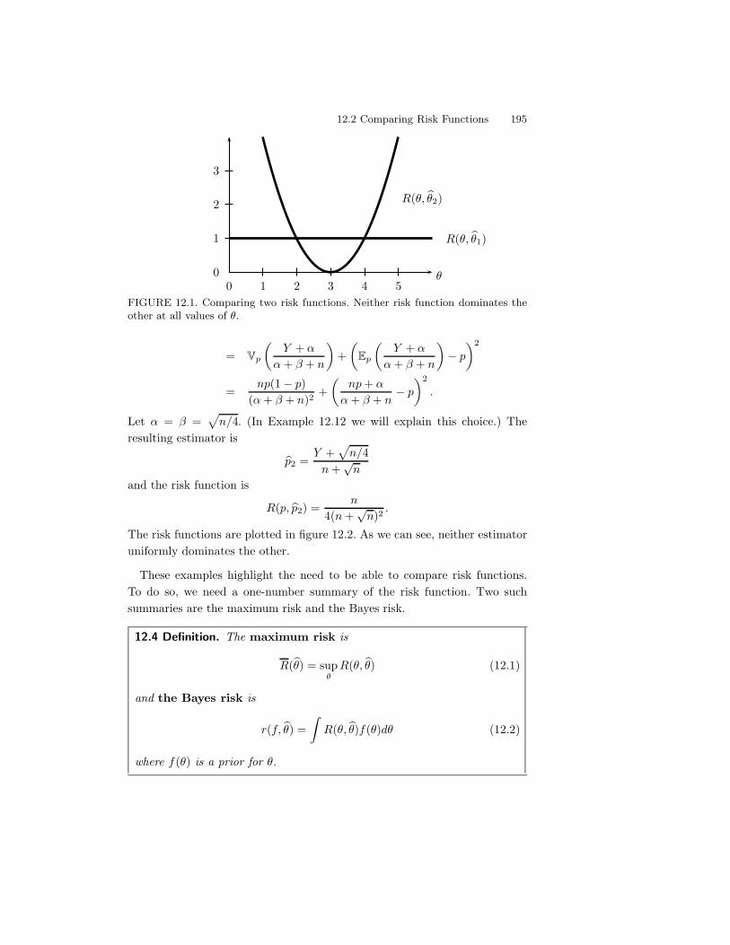
12.2 Comparing Risk Functions 195
0 1 2 3 4 50
1
2
3
R(0, 101)
R(0, 102)
0
FIGURE 12.1. Comparing two risk functions. Neither risk function dominates theother at all values of !.
= Vp
-Y + )
)+ ( + n
.+-
Ep
-Y + )
)+ ( + n
." p
.2
=np(1" p)
()+ ( + n)2+-
np + )
)+ ( + n" p
.2
.
Let ) = ( =3
n/4. (In Example 12.12 we will explain this choice.) Theresulting estimator is
1p2 =Y +
3n/4
n +/
n
and the risk function is
R(p, 1p2) =n
4(n +/
n)2.
The risk functions are plotted in figure 12.2. As we can see, neither estimatoruniformly dominates the other.
These examples highlight the need to be able to compare risk functions.To do so, we need a one-number summary of the risk function. Two suchsummaries are the maximum risk and the Bayes risk.
12.4 Definition. The maximum risk is
R(10) = sup(
R(0, 10) (12.1)
and the Bayes risk is
r(f, 10) =9
R(0, 10)f(0)d0 (12.2)
where f(0) is a prior for 0.
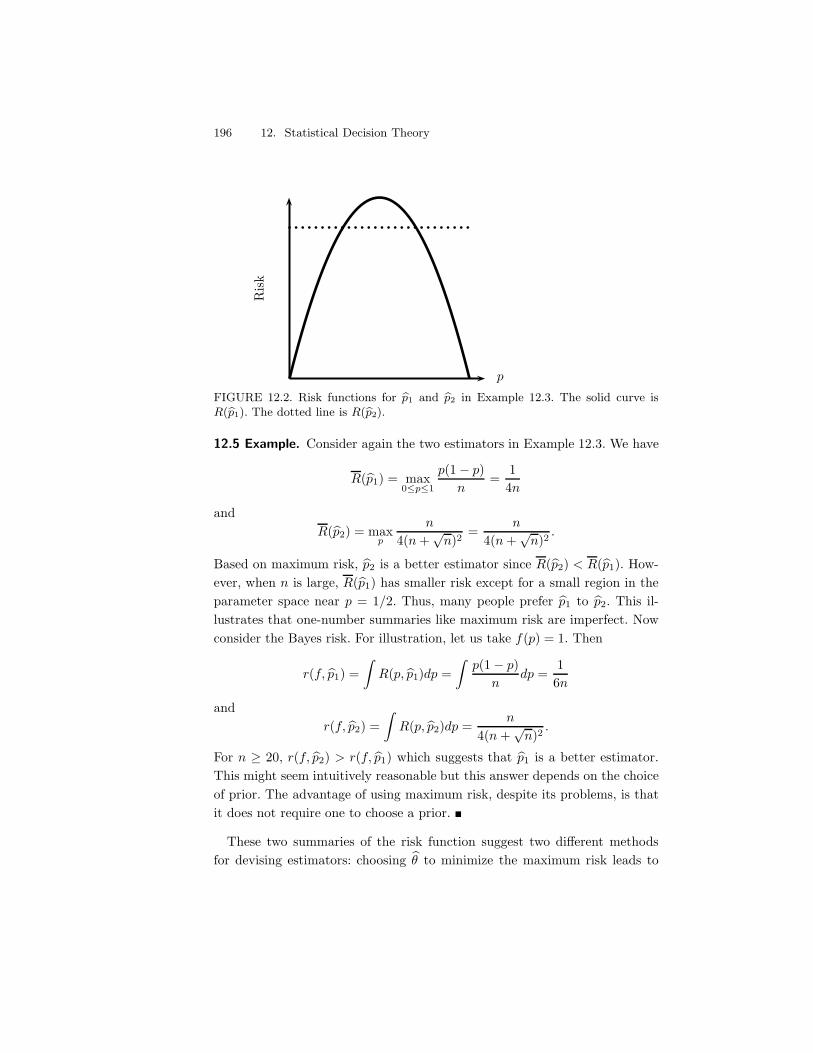
196 12. Statistical Decision Theory
Ris
k
p
FIGURE 12.2. Risk functions for 1p1 and 1p2 in Example 12.3. The solid curve isR(1p1). The dotted line is R(1p2).
12.5 Example. Consider again the two estimators in Example 12.3. We have
R(1p1) = max0%p%1
p(1" p)n
=14n
andR(1p2) = max
p
n
4(n +/
n)2=
n
4(n +/
n)2.
Based on maximum risk, 1p2 is a better estimator since R(1p2) < R(1p1). How-ever, when n is large, R(1p1) has smaller risk except for a small region in theparameter space near p = 1/2. Thus, many people prefer 1p1 to 1p2. This il-lustrates that one-number summaries like maximum risk are imperfect. Nowconsider the Bayes risk. For illustration, let us take f(p) = 1. Then
r(f, 1p1) =9
R(p, 1p1)dp =9
p(1" p)n
dp =16n
andr(f, 1p2) =
9R(p, 1p2)dp =
n
4(n +/
n)2.
For n * 20, r(f, 1p2) > r(f, 1p1) which suggests that 1p1 is a better estimator.This might seem intuitively reasonable but this answer depends on the choiceof prior. The advantage of using maximum risk, despite its problems, is thatit does not require one to choose a prior. !
These two summaries of the risk function suggest two di!erent methodsfor devising estimators: choosing 10 to minimize the maximum risk leads to
12.3 Bayes Estimators 197
minimax estimators; choosing 10 to minimize the Bayes risk leads to Bayesestimators.
12.6 Definition. A decision rule that minimizes the Bayes risk is called aBayes rule. Formally, 10 is a Bayes rule with respect to the prior f if
r(f, 10) = infc(
r(f, c0) (12.3)
where the infimum is over all estimators c0. An estimator that minimizesthe maximum risk is called a minimax rule. Formally, 10 is minimax if
sup(
R(0, 10) = infc(
sup(
R(0, c0) (12.4)
where the infimum is over all estimators c0.
12.3 Bayes Estimators
Let f be a prior. From Bayes’ theorem, the posterior density is
f(0|x) =f(x|0)f(0)
m(x)=
f(x|0)f(0)8f(x|0)f(0)d0
(12.5)
where m(x) =8
f(x, 0)d0 =8
f(x|0)f(0)d0 is the marginal distribution ofX . Define the posterior risk of an estimator 10(x) by
r(10|x) =9
L(0, 10(x))f(0|x)d0. (12.6)
12.7 Theorem. The Bayes risk r(f, 10) satisfies
r(f, 10) =9
r(10|x)m(x) dx.
Let 10(x) be the value of 0 that minimizes r(10|x). Then 10 is the Bayes estimator.
Proof. We can rewrite the Bayes risk as follows:
r(f, 10) =9
R(0, 10)f(0)d0 =9 (9
L(0, 10(x))f(x|0)dx
)f(0)d0
=9 9
L(0, 10(x))f(x, 0)dxd0 =9 9
L(0, 10(x))f(0|x)m(x)dxd0
=9 (9
L(0, 10(x))f(0|x)d0
)m(x) dx =
9r(10|x)m(x) dx.
198 12. Statistical Decision Theory
If we choose 10(x) to be the value of 0 that minimizes r(10|x) then we will mini-mize the integrand at every x and thus minimize the integral
8r(10|x)m(x)dx.
!
Now we can find an explicit formula for the Bayes estimator for some specificloss functions.
12.8 Theorem. If L(0, 10) = (0 " 10)2 then the Bayes estimator is
10(x) =90f(0|x)d0 = E(0|X = x). (12.7)
If L(0, 10) = |0 " 10| then the Bayes estimator is the median of the posteriorf(0|x). If L(0, 10) is zero–one loss, then the Bayes estimator is the mode of theposterior f(0|x).
Proof. We will prove the theorem for squared error loss. The Bayes rule10(x) minimizes r(10|x) =
8(0" 10(x))2f(0|x)d0. Taking the derivative of r(10|x)
with respect to 10(x) and setting it equal to 0 yields the equation 28(0 "
10(x))f(0|x)d0 = 0. Solving for 10(x) we get 12.7. !
12.9 Example. Let X1, . . . , Xn ! N(µ,#2) where #2 is known. Suppose weuse a N(a, b2) prior for µ. The Bayes estimator with respect to squared errorloss is the posterior mean, which is
10(X1, . . . , Xn) =b2
b2 + %2
n
X +%2
n
b2 + %2
n
a. !
12.4 Minimax Rules
Finding minimax rules is complicated and we cannot attempt a completecoverage of that theory here but we will mention a few key results. The mainmessage to take away from this section is: Bayes estimators with a constantrisk function are minimax.
12.10 Theorem. Let 10f be the Bayes rule for some prior f :
r(f, 10f ) = inf1(
r(f, 10). (12.8)
Suppose thatR(0, 10f ) , r(f, 10f ) for all 0. (12.9)
Then 10f is minimax and f is called a least favorable prior.
12.4 Minimax Rules 199
Proof. Suppose that 10f is not minimax. Then there is another rule 100 suchthat sup( R(0, 100) < sup( R(0, 10f ). Since the average of a function is alwaysless than or equal to its maximum, we have that r(f, 100) , sup( R(0, 100).Hence,
r(f, 100) , sup(
R(0, 100) < sup(
R(0, 10f ) , r(f, 10f )
which contradicts (12.8). !
12.11 Theorem. Suppose that 10 is the Bayes rule with respect to someprior f . Suppose further that 10 has constant risk: R(0, 10) = c for some c.Then 10 is minimax.
Proof. The Bayes risk is r(f, 10) =8
R(0, 10)f(0)d0 = c and hence R(0, 10) ,r(f, 10) for all 0. Now apply the previous theorem. !
12.12 Example. Consider the Bernoulli model with squared error loss. Inexample 12.3 we showed that the estimator
1p(Xn) =0n
i=1 Xi +3
n/4n +/
n
has a constant risk function. This estimator is the posterior mean, and hencethe Bayes rule, for the prior Beta(),() with ) = ( =
3n/4. Hence, by the
previous theorem, this estimator is minimax. !
12.13 Example. Consider again the Bernoulli but with loss function
L(p, 1p) =(p" 1p)2
p(1" p).
Let
1p(Xn) = 1p =0n
i=1 Xi
n.
The risk is
R(p, 1p) = E
-(1p" p)2
p(1" p)
.=
1p(1" p)
-p(1" p)
n
.=
1n
which, as a function of p, is constant. It can be shown that, for this lossfunction, 1p(Xn) is the Bayes estimator under the prior f(p) = 1. Hence, 1p isminimax. !
A natural question to ask is: what is the minimax estimator for a Normalmodel?
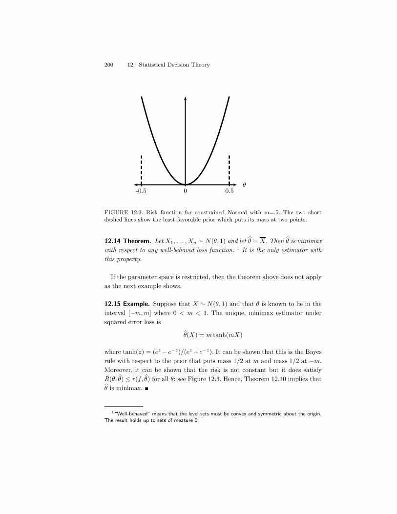
200 12. Statistical Decision Theory
00 0.5-0.5
FIGURE 12.3. Risk function for constrained Normal with m=.5. The two shortdashed lines show the least favorable prior which puts its mass at two points.
12.14 Theorem. Let X1, . . . , Xn ! N(0, 1) and let 10 = X. Then 10 is minimaxwith respect to any well-behaved loss function. 1 It is the only estimator withthis property.
If the parameter space is restricted, then the theorem above does not applyas the next example shows.
12.15 Example. Suppose that X ! N(0, 1) and that 0 is known to lie in theinterval ["m, m] where 0 < m < 1. The unique, minimax estimator undersquared error loss is
10(X) = m tanh(mX)
where tanh(z) = (ez" e$z)/(ez + e$z). It can be shown that this is the Bayesrule with respect to the prior that puts mass 1/2 at m and mass 1/2 at "m.Moreover, it can be shown that the risk is not constant but it does satisfyR(0, 10) , r(f, 10) for all 0; see Figure 12.3. Hence, Theorem 12.10 implies that10 is minimax. !
1“Well-behaved” means that the level sets must be convex and symmetric about the origin.The result holds up to sets of measure 0.
12.5 Maximum Likelihood, Minimax, and Bayes 201
12.5 Maximum Likelihood, Minimax, and Bayes
For parametric models that satisfy weak regularity conditions, the maximumlikelihood estimator is approximately minimax. Consider squared error losswhich is squared bias plus variance. In parametric models with large samples,it can be shown that the variance term dominates the bias so the risk of themle 10 roughly equals the variance:2
R(0, 10) = V((10) + bias2 . V((10).
As we saw in Chapter 9, the variance of the mle is approximately
V(10) . 1nI(0)
where I(0) is the Fisher information. Hence,
nR(0, 10) . 1I(0)
. (12.10)
For any other estimator 0&, it can be shown that for large n, R(0, 0&) * R(0, 10).More precisely,
lim&"0
lim supn"!
sup|($("|<&
n R(0&, 10) * 1I(0)
. (12.11)
This says that, in a local, large sample sense, the mle is minimax. It can alsobe shown that the mle is approximately the Bayes rule.
In summary:
In most parametric models, with large samples, the mle is approxi-
mately minimax and Bayes.
There is a caveat: these results break down when the number of parametersis large as the next example shows.
12.16 Example (Many Normal means). Let Yi ! N(0i,#2/n), i = 1, . . . , n.Let Y = (Y1, . . . , Yn) denote the data and let 0 = (01, . . . , 0n) denote theunknown parameters. Assume that
0 $ "n 0:
(01, . . . , 0n) :n*
i=1
02i , c2
Y
2Typically, the squared bias is order O(n!2) while the variance is of order O(n!1).
202 12. Statistical Decision Theory
for some c > 0. In this model, there are as many parameters as observations. 3
The mle is 10 = Y = (Y1, . . . , Yn). Under the loss function L(0, 10) =0n
i=1(10i"0i)2, the risk of the mle is R(0, 10) = #2. It can be shown that the minimax riskis approximately #2/(#2 + c2) and one can find an estimator c0 that achievesthis risk. Since #2/(#2 +c2) < #2, we see that c0 has smaller risk than the mle.In practice, the di!erence between the risks can be substantial. This showsthat maximum likelihood is not an optimal estimator in high dimensionalproblems. !
12.6 Admissibility
Minimax estimators and Bayes estimators are “good estimators” in the sensethat they have small risk. It is also useful to characterize bad estimators.
12.17 Definition. An estimator 10 is inadmissible if there exists anotherrule 10& such that
R(0, 10&) , R(0, 10) for all 0 and
R(0, 10&) < R(0, 10) for at least one 0.
Otherwise, 10 is admissible.
12.18 Example. Let X ! N(0, 1) and consider estimating 0 with squarederror loss. Let 10(X) = 3. We will show that 10 is admissible. Suppose not.Then there exists a di!erent rule 10& with smaller risk. In particular, R(3, 10&) ,R(3, 10) = 0. Hence, 0 = R(3, 10&) =
8(10&(x) " 3)2f(x; 3)dx. Thus, 10&(x) = 3.
So there is no rule that beats 10. Even though 10 is admissible it is clearly abad decision rule. !
12.19 Theorem (Bayes Rules Are Admissible). Suppose that " & R and thatR(0, 10) is a continuous function of 0 for every 10. Let f be a prior density withfull support, meaning that, for every 0 and every - > 0,
8 (+&($& f(0)d0 > 0. Let
10f be the Bayes’ rule. If the Bayes risk is finite then 10f is admissible.
Proof. Suppose 10f is inadmissible. Then there exists a better rule 10 suchthat R(0, 10) , R(0, 10f ) for all 0 and R(00, 10) < R(00, 10f ) for some 00. Let
3The many Normal means problem is more general than it looks. Many nonparametric esti-mation problems are mathematically equivalent to this model.
12.6 Admissibility 203
* = R(00, 10f ) " R(00, 10) > 0. Since R is continuous, there is an - > 0 suchthat R(0, 10f )"R(0, 10) > */2 for all 0 $ (00 " -, 00 + -). Now,
r(f, 10f )" r(f, 10) =9
R(0, 10f )f(0)d0 "9
R(0, 10)f(0)d0
=9 ?
R(0, 10f )"R(0, 10)@f(0)d0
*9 (0+&
(0$&
?R(0, 10f )"R(0, 10)
@f(0)d0
* *
2
9 (0+&
(0$&f(0)d0
> 0.
Hence, r(f, 10f ) > r(f, 10). This implies that 10f does not minimize r(f, 10) whichcontradicts the fact that 10f is the Bayes rule. !
12.20 Theorem. Let X1, . . . , Xn ! N(µ,#2). Under squared error loss, X isadmissible.
The proof of the last theorem is quite technical and is omitted but the ideais as follows: The posterior mean is admissible for any strictly positive prior.Take the prior to be N(a, b2). When b2 is very large, the posterior mean isapproximately equal to X.
How are minimaxity and admissibility linked? In general, a rule may be one,both, or neither. But here are some facts linking admissibility and minimaxity.
12.21 Theorem. Suppose that 10 has constant risk and is admissible. Then itis minimax.
Proof. The risk is R(0, 10) = c for some c. If 10 were not minimax thenthere exists a rule 10& such that
R(0, 10&) , sup(
R(0, 10&) < sup(
R(0, 10) = c.
This would imply that 10 is inadmissible. !
Now we can prove a restricted version of Theorem 12.14 for squared errorloss.
12.22 Theorem. Let X1, . . . , Xn ! N(0, 1). Then, under squared error loss,10 = X is minimax.
Proof. According to Theorem 12.20, 10 is admissible. The risk of 10 is 1/n
which is constant. The result follows from Theorem 12.21. !
204 12. Statistical Decision Theory
Although minimax rules are not guaranteed to be admissible they are “closeto admissible.” Say that 10 is strongly inadmissible if there exists a rule 10&
and an - > 0 such that R(0, 10&) < R(0, 10)" - for all 0.
12.23 Theorem. If 10 is minimax, then it is not strongly inadmissible.
12.7 Stein’s Paradox
Suppose that X ! N(0, 1) and consider estimating 0 with squared error loss.From the previous section we know that 10(X) = X is admissible. Now considerestimating two, unrelated quantities 0 = (01, 02) and suppose that X1 !N(01, 1) and X2 ! N(02, 1) independently, with loss L(0, 10) =
02j=1(0j"10j)2.
Not surprisingly, 10(X) = X is again admissible where X = (X1, X2). Nowconsider the generalization to k normal means. Let 0 = (01, . . . , 0k), X =(X1, . . . , Xk) with Xi ! N(0i, 1) (independent) and loss L(0, 10) =
0kj=1(0j "
10j)2. Stein astounded everyone when he proved that, if k * 3, then 10(X) = X
is inadmissible. It can be shown that the James-Stein estimator 10S hassmaller risk, where 10S = (10S
1 , . . . , 10Sk ),
10Si (X) =
-1" k " 20
i X2i
.+
Xi (12.12)
and (z)+ = max{z, 0}. This estimator shrinks the Xi’s towards 0. The messageis that, when estimating many parameters, there is great value in shrinking theestimates. This observation plays an important role in modern nonparametricfunction estimation.
12.8 Bibliographic Remarks
Aspects of decision theory can be found in Casella and Berger (2002), Berger(1985), Ferguson (1967), and Lehmann and Casella (1998).
12.9 Exercises
1. In each of the following models, find the Bayes risk and the Bayes esti-mator, using squared error loss.
(a) X ! Binomial(n, p), p ! Beta(),().
12.9 Exercises 205
(b) X ! Poisson(%), % ! Gamma(),().
(c) X ! N(0,#2) where #2 is known and 0 ! N(a, b2).
2. Let X1, . . . , Xn ! N(0,#2) and suppose we estimate 0 with loss functionL(0, 10) = (0 " 10)2/#2. Show that X is admissible and minimax.
3. Let " = {01, . . . , 0k} be a finite parameter space. Prove that the poste-rior mode is the Bayes estimator under zero–one loss.
4. (Casella and Berger (2002).) Let X1, . . . , Xn be a sample from a distri-bution with variance #2. Consider estimators of the form bS2 where S2
is the sample variance. Let the loss function for estimating #2 be
L(#2, 1#2) =1#2
#2" 1" log
-1#2
#2
..
Find the optimal value of b that minimizes the risk for all #2.
5. (Berliner (1983).) Let X ! Binomial(n, p) and suppose the loss functionis
L(p, 1p) =-
1" 1pp
.2
where 0 < p < 1. Consider the estimator 1p(X) = 0. This estimator fallsoutside the parameter space (0, 1) but we will allow this. Show that1p(X) = 0 is the unique, minimax rule.
6. (Computer Experiment.) Compare the risk of the mle and the James-Stein estimator (12.12) by simulation. Try various values of n and vari-ous vectors 0. Summarize your results.

This is page 206Printer: Opaque this
Part III
Statistical Models andMethods

This is pagePrinter: Opaque this
This is page 209Printer: Opaque this
13Linear and Logistic Regression
Regression is a method for studying the relationship between a responsevariable Y and a covariate X . The covariate is also called a predictorvariable or a feature. 1 One way to summarize the relationship between X
and Y is through the regression function
r(x) = E(Y |X = x) =9
y f(y|x)dy. (13.1)
Our goal is to estimate the regression function r(x) from data of the form
(Y1, X1), . . . , (Yn, Xn) ! FX,Y .
In this Chapter, we take a parametric approach and assume that r is linear.In Chapters 20 and 21 we discuss nonparametric regression.
13.1 Simple Linear Regression
The simplest version of regression is when Xi is simple (one-dimensional) andr(x) is assumed to be linear:
r(x) = (0 + (1x.
1The term “regression” is due to Sir Francis Galton (1822-1911) who noticed that tall andshort men tend to have sons with heights closer to the mean. He called this “regression towardsthe mean.”
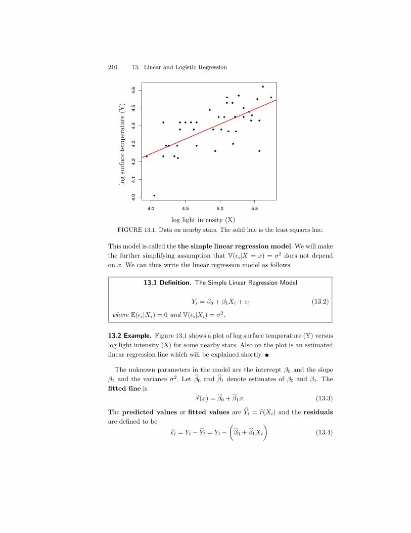
210 13. Linear and Logistic Regression
4.0 4.5 5.0 5.5
4.0
4.1
4.2
4.3
4.4
4.5
4.6
log
surf
ace
tem
pera
ture
(Y)
log light intensity (X)FIGURE 13.1. Data on nearby stars. The solid line is the least squares line.
This model is called the the simple linear regression model. We will makethe further simplifying assumption that V(-i|X = x) = #2 does not dependon x. We can thus write the linear regression model as follows.
13.1 Definition. The Simple Linear Regression Model
Yi = (0 + (1Xi + -i (13.2)
where E(-i|Xi) = 0 and V(-i|Xi) = #2.
13.2 Example. Figure 13.1 shows a plot of log surface temperature (Y) versuslog light intensity (X) for some nearby stars. Also on the plot is an estimatedlinear regression line which will be explained shortly. !
The unknown parameters in the model are the intercept (0 and the slope(1 and the variance #2. Let 1(0 and 1(1 denote estimates of (0 and (1. Thefitted line is
1r(x) = 1(0 + 1(1x. (13.3)
The predicted values or fitted values are 1Yi = 1r(Xi) and the residualsare defined to be
1-i = Yi " 1Yi = Yi "-1(0 + 1(1Xi
.. (13.4)
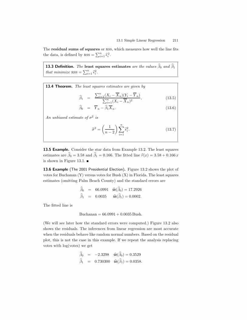
13.1 Simple Linear Regression 211
The residual sums of squares or rss, which measures how well the line fitsthe data, is defined by rss =
0ni=1 1- 2
i .
13.3 Definition. The least squares estimates are the values 1(0 and 1(1
that minimize rss =0n
i=1 1-2i .
13.4 Theorem. The least squares estimates are given by
1(1 =0n
i=1(Xi "Xn)(Yi " Y n)0n
i=1(Xi "Xn)2, (13.5)
1(0 = Y n " 1(1Xn. (13.6)
An unbiased estimate of #2 is
1#2 =-
1n" 2
. n*
i=1
1-2i . (13.7)
13.5 Example. Consider the star data from Example 13.2. The least squaresestimates are 1(0 = 3.58 and 1(1 = 0.166. The fitted line 1r(x) = 3.58 + 0.166 x
is shown in Figure 13.1. !
13.6 Example (The 2001 Presidential Election). Figure 13.2 shows the plot ofvotes for Buchanan (Y) versus votes for Bush (X) in Florida. The least squaresestimates (omitting Palm Beach County) and the standard errors are
1(0 = 66.0991 1se(1(0) = 17.29261(1 = 0.0035 1se(1(1) = 0.0002.
The fitted line is
Buchanan = 66.0991 + 0.0035 Bush.
(We will see later how the standard errors were computed.) Figure 13.2 alsoshows the residuals. The inferences from linear regression are most accuratewhen the residuals behave like random normal numbers. Based on the residualplot, this is not the case in this example. If we repeat the analysis replacingvotes with log(votes) we get
1(0 = "2.3298 1se(1(0) = 0.35291(1 = 0.730300 1se(1(1) = 0.0358.
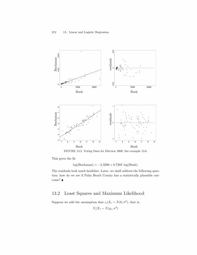
212 13. Linear and Logistic Regression
0 125000 250000
01
50
03
00
0
0 125000 250000!5
00
05
00
7 8 9 10 11 12 13
23
45
67
8
7 8 9 10 11 12 13
!1
01
Bush
Buc
hana
n
Bush
resi
dual
s
Bush
Buc
hana
n
Bush
resi
dual
s
FIGURE 13.2. Voting Data for Election 2000. See example 13.6.
This gives the fit
log(Buchanan) = "2.3298 + 0.7303 log(Bush).
The residuals look much healthier. Later, we shall address the following ques-tion: how do we see if Palm Beach County has a statistically plausible out-come? !
13.2 Least Squares and Maximum Likelihood
Suppose we add the assumption that -i|Xi ! N(0,#2), that is,
Yi|Xi ! N(µi,#2)
13.2 Least Squares and Maximum Likelihood 213
where µi = (0 + (1Xi. The likelihood function is
n/
i=1
f(Xi, Yi) =n/
i=1
fX(Xi)fY |X(Yi|Xi)
=n/
i=1
fX(Xi)-n/
i=1
fY |X(Yi|Xi)
= L1 - L2
where L1 =Dn
i=1 fX(Xi) and
L2 =n/
i=1
fY |X(Yi|Xi). (13.8)
The term L1 does not involve the parameters (0 and (1. We shall focus onthe second term L2 which is called the conditional likelihood, given by
L2 0 L((0,(1,#) =n/
i=1
fY |X(Yi|Xi) 3 #$n exp
:" 1
2#2
*
i
(Yi " µi)2Y
.
The conditional log-likelihood is
4((0,(1,#) = "n log# " 12#2
n*
i=1
-Yi " ((0 + (1Xi)
.2
. (13.9)
To find the mle of ((0,(1) we maximize 4((0,(1,#). From (13.9) we see that
maximizing the likelihood is the same as minimizing the rss0n
i=1
-Yi"((0+
(1Xi).2
. Therefore, we have shown the following:
13.7 Theorem. Under the assumption of Normality, the least squares estima-tor is also the maximum likelihood estimator.
We can also maximize 4((0,(1,#) over #, yielding the mle
1#2 =1n
*
i
1- 2i . (13.10)
This estimator is similar to, but not identical to, the unbiased estimator.Common practice is to use the unbiased estimator (13.7).
214 13. Linear and Logistic Regression
13.3 Properties of the Least Squares Estimators
We now record the standard errors and limiting distribution of the leastsquares estimator. In regression problems, we usually focus on the proper-ties of the estimators conditional on Xn = (X1, . . . , Xn). Thus, we state themeans and variances as conditional means and variances.
13.8 Theorem. Let 1(T = (1(0, 1(1)T denote the least squares estimators.Then,
E(1(|Xn) =-(0
(1
.
V(1(|Xn) =#2
n s2X
(1n
0ni=1 X2
i "Xn
"Xn 1
)(13.11)
where s2X = n$1
0ni=1(Xi "Xn)2.
The estimated standard errors of 1(0 and 1(1 are obtained by taking thesquare roots of the corresponding diagonal terms of V(1(|Xn) and insertingthe estimate 1# for #. Thus,
1se(1(0) =1#
sX/
n
U0ni=1 X2
i
n(13.12)
1se(1(1) =1#
sX/
n. (13.13)
We should really write these as 1se(1(0|Xn) and 1se(1(1|Xn) but we will use theshorter notation 1se(1(0) and 1se(1(1).
13.9 Theorem. Under appropriate conditions we have:
1. (Consistency): 1(0P")(0 and 1(1
P")(1.
2. (Asymptotic Normality):
1(0 " (0
1se(1(0)! N(0, 1) and
1(1 " (1
1se(1(1)! N(0, 1).
3. Approximate 1" ) confidence intervals for (0 and (1 are
1(0 ± z#/2 1se(1(0) and 1(1 ± z#/2 1se(1(1). (13.14)
13.4 Prediction 215
4. The Wald test 2 for testing H0 : (1 = 0 versus H1 : (1 (= 0 is: reject H0
if |W | > z#/2 where W = 1(1/1se(1(1).
13.10 Example. For the election data, on the log scale, a 95 percent confi-dence interval is .7303 ± 2(.0358) = (.66, .80). The Wald statistics for testingH0 : (1 = 0 versus H1 : (1 (= 0 is |W | = |.7303 " 0|/.0358 = 20.40 with ap-value of P(|Z| > 20.40) . 0. This is strong evidence that that the true slopeis not 0. !
13.4 Prediction
Suppose we have estimated a regression model 1r(x) = 1(0 + 1(1x from data(X1, Y1), . . . , (Xn, Yn). We observe the value X = x* of the covariate for anew subject and we want to predict their outcome Y*. An estimate of Y* is
1Y* = 1(0 + 1(1x*. (13.15)
Using the formula for the variance of the sum of two random variables,
V(1Y*) = V(1(0 + 1(1x*) = V(1(0) + x2*V(1(1) + 2x*Cov(1(0, 1(1).
Theorem 13.8 gives the formulas for all the terms in this equation. The es-timated standard error 1se(1Y*) is the square root of this variance, with 1#2 inplace of #2. However, the confidence interval for Y* is not of the usual form1Y* ± z#/2 1se. The reason for this is explained in Exercise 10. The correct formof the confidence interval is given in the following theorem.
13.11 Theorem (Prediction Interval). Let
1. 2n = 1#2
-0ni=1(Xi "X*)2
n0
i(Xi "X)2+ 1.
. (13.16)
An approximate 1" ) prediction interval for Y* is
1Y* ± z#/21.n. (13.17)
2Recall from equation (10.5) that the Wald statistic for testing H0 : β = β0 versus H1 :β %= β0 is W = (1β " β0)/1se(1β).
216 13. Linear and Logistic Regression
13.12 Example (Election Data Revisited). On the log scale, our linear regres-sion gives the following prediction equation:
log(Buchanan) = "2.3298 + 0.7303 log(Bush).
In Palm Beach, Bush had 152,954 votes and Buchanan had 3,467 votes. On thelog scale this is 11.93789 and 8.151045. How likely is this outcome, assumingour regression model is appropriate? Our prediction for log Buchanan votes-2.3298 + .7303 (11.93789)=6.388441. Now, 8.151045 is bigger than 6.388441but is it “significantly” bigger? Let us compute a confidence interval. Wefind that 1.n = .093775 and the approximate 95 percent confidence interval is(6.200,6.578) which clearly excludes 8.151. Indeed, 8.151 is nearly 20 standarderrors from 1Y*. Going back to the vote scale by exponentiating, the confidenceinterval is (493,717) compared to the actual number of votes which is 3,467.!
13.5 Multiple Regression
Now suppose that the covariate is a vector of length k. The data are of theform
(Y1, X1), . . . , (Yi, Xi), . . . , (Yn, Xn)
where
Xi = (Xi1, . . . , Xik).
Here, Xi is the vector of k covariate values for the ith observation. The linearregression model is
Yi =k*
j=1
(jXij + -i (13.18)
for i = 1, . . . , n, where E(-i|X1i, . . . , Xki) = 0. Usually we want to include anintercept in the model which we can do by setting Xi1 = 1 for i = 1, . . . , n. Atthis point it will be more convenient to express the model in matrix notation.The outcomes will be denoted by
Y =
E
FFFG
Y1
Y2...
Yn
H
IIIJ
13.5 Multiple Regression 217
and the covariates will be denoted by
X =
E
FFFG
X11 X12 . . . X1k
X21 X22 . . . X2k...
......
...Xn1 Xn2 . . . Xnk
H
IIIJ.
Each row is one observation; the columns correspond to the k covariates. Thus,X is a (n- k) matrix. Let
( =
E
FG(1...(k
H
IJ and - =
E
FG-1...-n
H
IJ .
Then we can write (13.18) as
Y = X( + -. (13.19)
The form of the least squares estimate is given in the following theorem.
13.13 Theorem. Assuming that the (k - k) matrix XT X is invertible,
1( = (XT X)$1XT Y (13.20)
V(1(|Xn) = #2(XT X)$1 (13.21)1( . N((,#2(XT X)$1). (13.22)
The estimate regression function is 1r(x) =0k
j=11(jxj . An unbiased esti-
mate of #2 is
1#2 =-
1n" k
. n*
i=1
1- 2i
where 1- = X 1("Y is the vector of residuals. An approximate 1") confidenceinterval for (j is
1(j ± z#/2 1se(1(j) (13.23)
where 1se2(1(j) is the jth diagonal element of the matrix 1#2 (XT X)$1.
13.14 Example. Crime data on 47 states in 1960 can be obtained fromhttp://lib.stat.cmu.edu/DASL/Stories/USCrime.html.
If we fit a linear regression of crime rate on 10 variables we get the following:
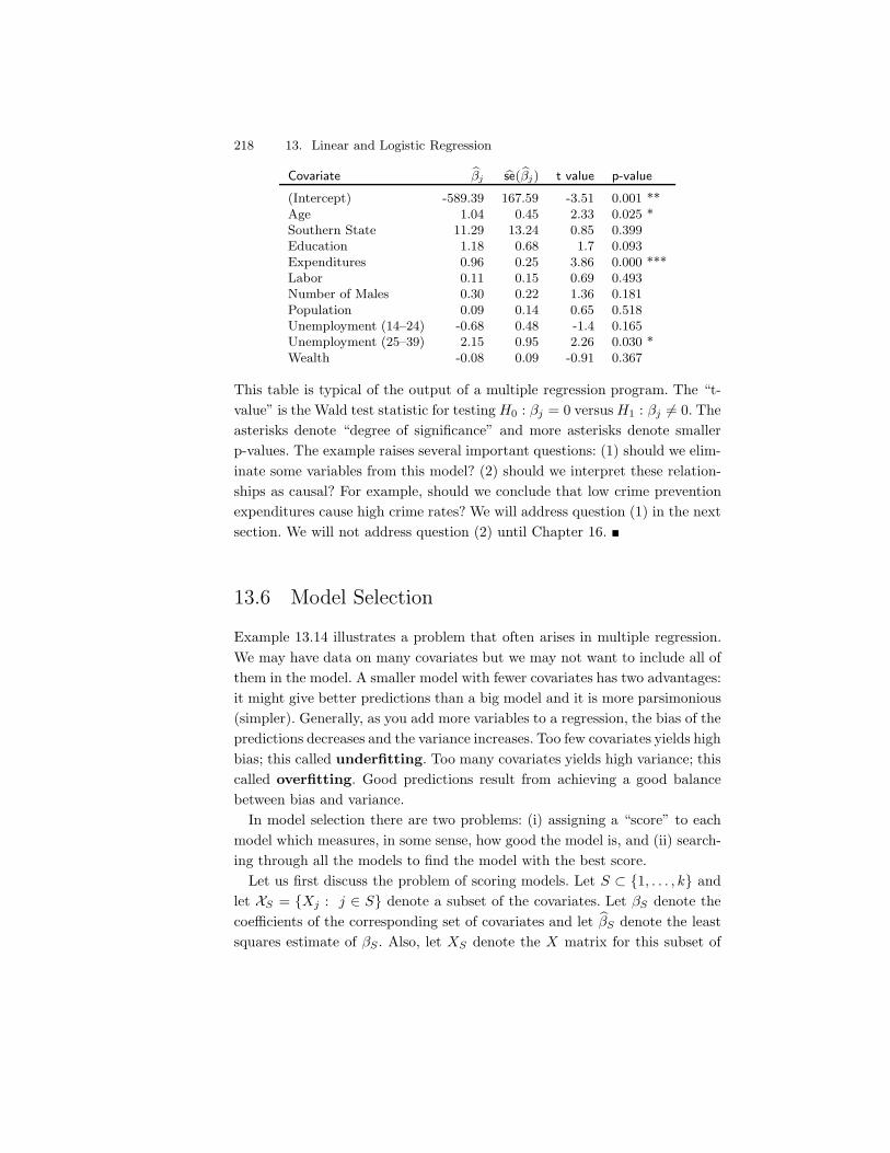
218 13. Linear and Logistic Regression
Covariate 1"j 1se(1"j) t value p-value
(Intercept) -589.39 167.59 -3.51 0.001 **Age 1.04 0.45 2.33 0.025 *Southern State 11.29 13.24 0.85 0.399Education 1.18 0.68 1.7 0.093Expenditures 0.96 0.25 3.86 0.000 ***Labor 0.11 0.15 0.69 0.493Number of Males 0.30 0.22 1.36 0.181Population 0.09 0.14 0.65 0.518Unemployment (14–24) -0.68 0.48 -1.4 0.165Unemployment (25–39) 2.15 0.95 2.26 0.030 *Wealth -0.08 0.09 -0.91 0.367
This table is typical of the output of a multiple regression program. The “t-value” is the Wald test statistic for testing H0 : (j = 0 versus H1 : (j (= 0. Theasterisks denote “degree of significance” and more asterisks denote smallerp-values. The example raises several important questions: (1) should we elim-inate some variables from this model? (2) should we interpret these relation-ships as causal? For example, should we conclude that low crime preventionexpenditures cause high crime rates? We will address question (1) in the nextsection. We will not address question (2) until Chapter 16. !
13.6 Model Selection
Example 13.14 illustrates a problem that often arises in multiple regression.We may have data on many covariates but we may not want to include all ofthem in the model. A smaller model with fewer covariates has two advantages:it might give better predictions than a big model and it is more parsimonious(simpler). Generally, as you add more variables to a regression, the bias of thepredictions decreases and the variance increases. Too few covariates yields highbias; this called underfitting. Too many covariates yields high variance; thiscalled overfitting. Good predictions result from achieving a good balancebetween bias and variance.
In model selection there are two problems: (i) assigning a “score” to eachmodel which measures, in some sense, how good the model is, and (ii) search-ing through all the models to find the model with the best score.
Let us first discuss the problem of scoring models. Let S & {1, . . . , k} andlet XS = {Xj : j $ S} denote a subset of the covariates. Let (S denote thecoe#cients of the corresponding set of covariates and let 1(S denote the leastsquares estimate of (S . Also, let XS denote the X matrix for this subset of
13.6 Model Selection 219
covariates and define 1rS(x) to be the estimated regression function. The pre-dicted values from model S are denoted by 1Yi(S) = 1rS(Xi). The predictionrisk is defined to be
R(S) =n*
i=1
E(1Yi(S)" Y *i )2 (13.24)
where Y *i denotes the value of a future observation of Yi at covariate value
Xi. Our goal is to choose S to make R(S) small.The training error is defined to be
1Rtr(S) =n*
i=1
(1Yi(S)" Yi)2.
This estimate is very biased as an estimate of R(S).
13.15 Theorem. The training error is a downward-biased estimate of the pre-diction risk:
E( 1Rtr(S)) < R(S).
In fact,
bias( 1Rtr(S)) = E( 1Rtr(S))"R(S) = "2*
i=1
Cov(1Yi, Yi). (13.25)
The reason for the bias is that the data are being used twice: to estimatethe parameters and to estimate the risk. When we fit a complex model withmany parameters, the covariance Cov(1Yi, Yi) will be large and the bias of thetraining error gets worse. Here are some better estimates of risk.
Mallow’s Cp statistic is defined by
1R(S) = 1Rtr(S) + 2|S|1#2 (13.26)
where |S| denotes the number of terms in S and 1#2 is the estimate of #2
obtained from the full model (with all covariates in the model). This is simplythe training error plus a bias correction. This estimate is named in honor ofColin Mallows who invented it. The first term in (13.26) measures the fit ofthe model while the second measure the complexity of the model. Think ofthe Cp statistic as:
lack of fit + complexity penalty.
Thus, finding a good model involves trading o" fit and complexity.
220 13. Linear and Logistic Regression
A related method for estimating risk is AIC (Akaike Information Cri-terion). The idea is to choose S to maximize
4S " |S| (13.27)
where 4S is the log-likelihood of the model evaluated at the mle. 3 This canbe thought of “goodness of fit” minus “complexity.” In linear regression withNormal errors (and taking # equal to its estimate from the largest model),maximizing AIC is equivalent to minimizing Mallow’s Cp; see Exercise 8. Theappendix contains more explanation about AIC.
Yet another method for estimating risk is leave-one-out cross-validation.In this case, the risk estimator is
1RCV (S) =n*
i=1
(Yi " 1Y(i))2 (13.28)
where 1Y(i) is the prediction for Yi obtained by fitting the model with Yi omit-ted. It can be shown that
1RCV (S) =n*
i=1
(Yi " 1Yi(S)1" Uii(S)
)2
(13.29)
where Uii(S) is the ith diagonal element of the matrix
U(S) = XS(XTS XS)$1XT
S . (13.30)
Thus, one need not actually drop each observation and re-fit the model. Ageneralization is k-fold cross-validation. Here we divide the data into k
groups; often people take k = 10. We omit one group of data and fit themodels to the remaining data. We use the fitted model to predict the datain the group that was omitted. We then estimate the risk by
0i(Yi " 1Yi)2
where the sum is over the the data points in the omitted group. This process isrepeated for each of the k groups and the resulting risk estimates are averaged.
For linear regression, Mallows Cp and cross-validation often yield essentiallythe same results so one might as well use Mallows’ method. In some of themore complex problems we will discuss later, cross-validation will be moreuseful.
Another scoring method is BIC (Bayesian information criterion). Here wechoose a model to maximize
BIC(S) = 4S "|S|2
log n. (13.31)
3Some texts use a slightly di!erent definition of AIC which involves multiplying the definitionhere by 2 or -2. This has no e!ect on which model is selected.

13.6 Model Selection 221
The BIC score has a Bayesian interpretation. Let S = {S1, . . . , Sm} denotea set of models. Suppose we assign the prior P(Sj) = 1/m over the models.Also, assume we put a smooth prior on the parameters within each model. Itcan be shown that the posterior probability for a model is approximately,
P(Sj |data) . eBIC(Sj)
0r eBIC(Sr)
.
Hence, choosing the model with highest BIC is like choosing the model withhighest posterior probability. The BIC score also has an information-theoreticinterpretation in terms of something called minimum description length. TheBIC score is identical to Mallows Cp except that it puts a more severe penaltyfor complexity. It thus leads one to choose a smaller model than the othermethods.
Now let us turn to the problem of model search. If there are k covariatesthen there are 2k possible models. We need to search through all these models,assign a score to each one, and choose the model with the best score. If k isnot too large we can do a complete search over all the models. When k is large,this is infeasible. In that case we need to search over a subset of all the models.Two common methods are forward and backward stepwise regression.In forward stepwise regression, we start with no covariates in the model. Wethen add the one variable that leads to the best score. We continue addingvariables one at a time until the score does not improve. Backwards stepwiseregression is the same except that we start with the biggest model and dropone variable at a time. Both are greedy searches; nether is guaranteed tofind the model with the best score. Another popular method is to do randomsearching through the set of all models. However, there is no reason to expectthis to be superior to a deterministic search.
13.16 Example. We applied backwards stepwise regression to the crime datausing AIC. The following was obtained from the program R. This programuses a slightly di!erent definition of AIC. With their definition, we seek thesmallest (not largest) possible AIC. This is the same is minimizing MallowsCp.
The full model (which includes all covariates) has AIC= 310.37. In ascend-ing order, the AIC scores for deleting one variable are as follows:
variable Pop Labor South Wealth Males U1 Educ. U2 Age ExpendAIC 308 309 309 309 310 310 312 314 315 324
For example, if we dropped Pop from the model and kept the other terms,then the AIC score would be 308. Based on this information we drop “pop-
222 13. Linear and Logistic Regression
ulation” from the model and the current AIC score is 308. Now we considerdropping a variable from the current model. The AIC scores are:
variable South Labor Wealth Males U1 Education U2 Age ExpendAIC 308 308 308 309 309 310 313 313 329
We then drop “Southern” from the model. This process is continued untilthere is no gain in AIC by dropping any variables. In the end, we are left withthe following model:
Crime = 1.2 Age + .75 Education + .87 Expenditure
+ .34 Males " .86 U1 + 2.31 U2.
Warning! This does not yet address the question of which variables arecauses of crime. !
There is another method for model selection that avoids having to searchthrough all possible models. This method, which is due to Zheng and Loh(1995), does not seek to minimize prediction errors. Rather, it assumes somesubset of the (j ’s are exactly equal to 0 and tries to find the true model,that is, the smallest sub-model consisting of nonzero (j terms. The methodis carried out as follows.
Zheng-Loh Model Selection Method 4
1. Fit the full model with all k covariates and let Wj = 1(j/1se(1(j) denotethe Wald test statistic for H0 : (j = 0 versus H1 : (j (= 0.
2. Order the test statistics from largest to smallest in absolute value:
|W(1)| * |W(2)| * · · · * |W(k)|.
3. Let 1j be the value of j that minimizes
rss(j) + j 1#2 log n
where rss(j) is the residual sums of squares from the model withthe j largest Wald statistics.
4. Choose, as the final model, the regression with the 1j terms with thelargest absolute Wald statistics.
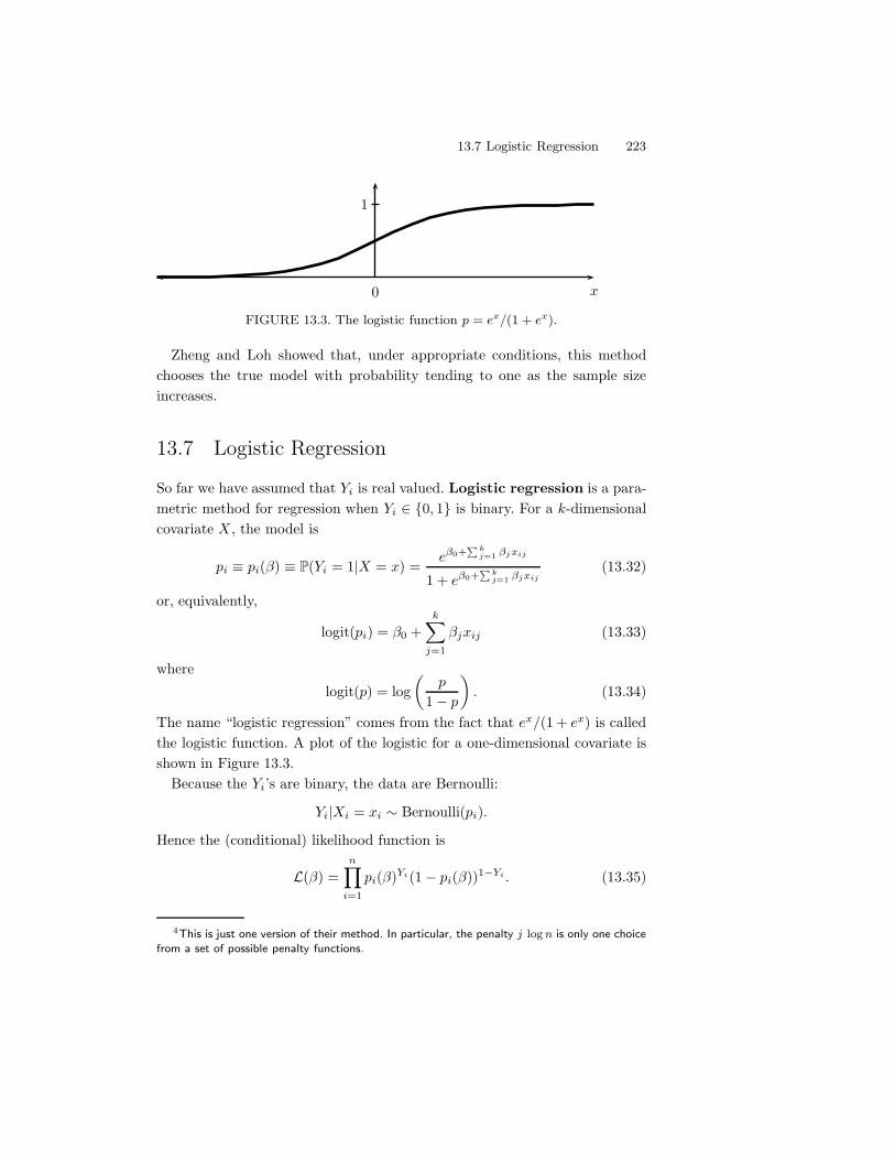
13.7 Logistic Regression 223
x0
1
FIGURE 13.3. The logistic function p = ex/(1 + ex).
Zheng and Loh showed that, under appropriate conditions, this methodchooses the true model with probability tending to one as the sample sizeincreases.
13.7 Logistic Regression
So far we have assumed that Yi is real valued. Logistic regression is a para-metric method for regression when Yi $ {0, 1} is binary. For a k-dimensionalcovariate X , the model is
pi 0 pi(() 0 P(Yi = 1|X = x) =e"0+
0kj=1 "jxij
1 + e"0+0k
j=1 "jxij(13.32)
or, equivalently,
logit(pi) = (0 +k*
j=1
(jxij (13.33)
wherelogit(p) = log
-p
1" p
.. (13.34)
The name “logistic regression” comes from the fact that ex/(1 + ex) is calledthe logistic function. A plot of the logistic for a one-dimensional covariate isshown in Figure 13.3.
Because the Yi’s are binary, the data are Bernoulli:
Yi|Xi = xi ! Bernoulli(pi).
Hence the (conditional) likelihood function is
L(() =n/
i=1
pi(()Yi(1" pi(())1$Yi . (13.35)
4This is just one version of their method. In particular, the penalty j log n is only one choicefrom a set of possible penalty functions.
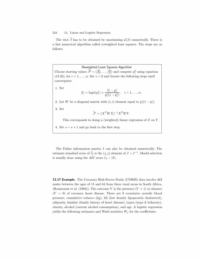
224 13. Linear and Logistic Regression
The mle 1( has to be obtained by maximizing L(() numerically. There isa fast numerical algorithm called reweighted least squares. The steps are asfollows:
Reweighted Least Squares Algorithm
Choose starting values 1(0 = (1(00 , . . . , 1(0
k) and compute p0i using equation
(13.32), for i = 1, . . . , n. Set s = 0 and iterate the following steps untilconvergence.
1. SetZi = logit(ps
i ) +Yi " ps
i
psi (1 " ps
i ), i = 1, . . . , n.
2. Let W be a diagonal matrix with (i, i) element equal to psi (1" ps
i ).
3. Set1(s = (XT WX)$1XT WY.
This corresponds to doing a (weighted) linear regression of Z on Y .
4. Set s = s + 1 and go back to the first step.
The Fisher information matrix I can also be obtained numerically. Theestimate standard error of 1(j is the (j, j) element of J = I$1. Model selectionis usually done using the AIC score 4S " |S|.
13.17 Example. The Coronary Risk-Factor Study (CORIS) data involve 462males between the ages of 15 and 64 from three rural areas in South Africa,(Rousseauw et al. (1983)). The outcome Y is the presence (Y = 1) or absence(Y = 0) of coronary heart disease. There are 9 covariates: systolic bloodpressure, cumulative tobacco (kg), ldl (low density lipoprotein cholesterol),adiposity, famhist (family history of heart disease), typea (type-A behavior),obesity, alcohol (current alcohol consumption), and age. A logistic regressionyields the following estimates and Wald statistics Wj for the coe#cients:
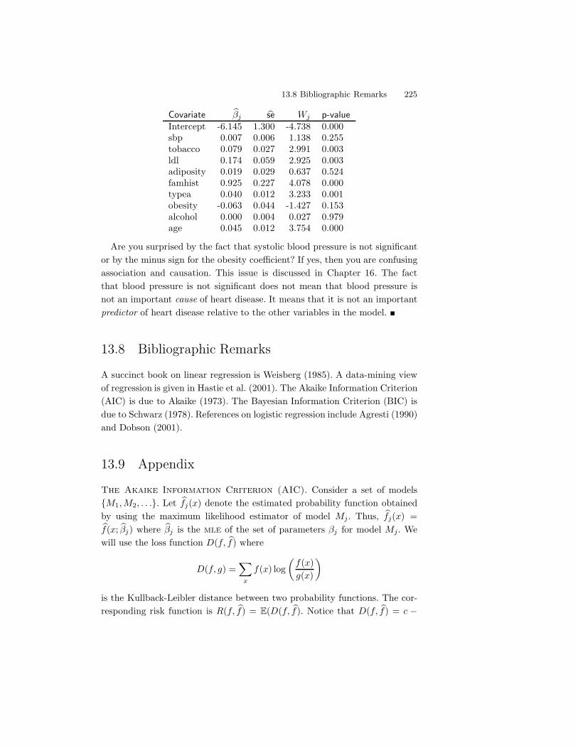
13.8 Bibliographic Remarks 225
Covariate 1(j 1se Wj p-valueIntercept -6.145 1.300 -4.738 0.000sbp 0.007 0.006 1.138 0.255tobacco 0.079 0.027 2.991 0.003ldl 0.174 0.059 2.925 0.003adiposity 0.019 0.029 0.637 0.524famhist 0.925 0.227 4.078 0.000typea 0.040 0.012 3.233 0.001obesity -0.063 0.044 -1.427 0.153alcohol 0.000 0.004 0.027 0.979age 0.045 0.012 3.754 0.000
Are you surprised by the fact that systolic blood pressure is not significantor by the minus sign for the obesity coe#cient? If yes, then you are confusingassociation and causation. This issue is discussed in Chapter 16. The factthat blood pressure is not significant does not mean that blood pressure isnot an important cause of heart disease. It means that it is not an importantpredictor of heart disease relative to the other variables in the model. !
13.8 Bibliographic Remarks
A succinct book on linear regression is Weisberg (1985). A data-mining viewof regression is given in Hastie et al. (2001). The Akaike Information Criterion(AIC) is due to Akaike (1973). The Bayesian Information Criterion (BIC) isdue to Schwarz (1978). References on logistic regression include Agresti (1990)and Dobson (2001).
13.9 Appendix
The Akaike Information Criterion (AIC). Consider a set of models{M1, M2, . . .}. Let 1fj(x) denote the estimated probability function obtainedby using the maximum likelihood estimator of model Mj. Thus, 1fj(x) =1f(x; 1(j) where 1(j is the mle of the set of parameters (j for model Mj. Wewill use the loss function D(f, 1f) where
D(f, g) =*
x
f(x) log-
f(x)g(x)
.
is the Kullback-Leibler distance between two probability functions. The cor-responding risk function is R(f, 1f) = E(D(f, 1f). Notice that D(f, 1f) = c "
226 13. Linear and Logistic Regression
A(f, 1f) where c =0
x f(x) log f(x) does not depend on 1f and
A(f, 1f) =*
x
f(x) log 1f(x).
Thus, minimizing the risk is equivalent to maximizing a(f, 1f) 0 E(A(f, 1f )).It is tempting to estimate a(f, 1f) by
0x1f(x) log 1f(x) but, just as the train-
ing error in regression is a highly biased estimate of prediction risk, it is alsothe case that
0x1f(x) log 1f(x) is a highly biased estimate of a(f, 1f). In fact,
the bias is approximately equal to |Mj|. Thus:
13.18 Theorem. AIC(Mj) is an approximately unbiased estimate of a(f, 1f).
13.10 Exercises
1. Prove Theorem 13.4.
2. Prove the formulas for the standard errors in Theorem 13.8. You shouldregard the Xi’s as fixed constants.
3. Consider the regression through the origin model:
Yi = (Xi + -.
Find the least squares estimate for (. Find the standard error of theestimate. Find conditions that guarantee that the estimate is consistent.
4. Prove equation (13.25).
5. In the simple linear regression model, construct a Wald test for H0 :(1 = 17(0 versus H1 : (1 (= 17(0.
6. Get the passenger car mileage data from
http://lib.stat.cmu.edu/DASL/Datafiles/carmpgdat.html
(a) Fit a simple linear regression model to predict MPG (miles pergallon) from HP (horsepower). Summarize your analysis including aplot of the data with the fitted line.
(b) Repeat the analysis but use log(MPG) as the response. Comparethe analyses.
13.10 Exercises 227
7. Get the passenger car mileage data from
http://lib.stat.cmu.edu/DASL/Datafiles/carmpgdat.html
(a) Fit a multiple linear regression model to predict MPG (miles pergallon) from the other variables. Summarize your analysis.
(b) Use Mallow Cp to select a best sub-model. To search through themodels try (i) forward stepwise, (ii) backward stepwise. Summarize yourfindings.
(c) Use the Zheng-Loh model selection method and compare to (b).
(d) Perform all possible regressions. Compare Cp and BIC. Compare theresults.
8. Assume a linear regression model with Normal errors. Take # known.Show that the model with highest AIC (equation (13.27)) is the modelwith the lowest Mallows Cp statistic.
9. In this question we will take a closer look at the AIC method. LetX1, . . . , Xn be iid observations. Consider two models M0 and M1. Un-der M0 the data are assumed to be N(0, 1) while under M1 the dataare assumed to be N(0, 1) for some unknown 0 $ R:
M0 : X1, . . . , Xn ! N(0, 1)
M1 : X1, . . . , Xn ! N(0, 1), 0 $ R.
This is just another way to view the hypothesis testing problem: H0 :0 = 0 versus H1 : 0 (= 0. Let 4n(0) be the log-likelihood function.The AIC score for a model is the log-likelihood at the mle minus thenumber of parameters. (Some people multiply this score by 2 but thatis irrelevant.) Thus, the AIC score for M0 is AIC0 = 4n(0) and the AICscore for M1 is AIC1 = 4n(10) " 1. Suppose we choose the model withthe highest AIC score. Let Jn denote the selected model:
Jn ='
0 if AIC0 > AIC1
1 if AIC1 > AIC0.
(a) Suppose that M0 is the true model, i.e. 0 = 0. Find
limn"!
P (Jn = 0) .
Now compute limn"! P (Jn = 0) when 0 (= 0.
228 13. Linear and Logistic Regression
(b) The fact that limn"! P (Jn = 0) (= 1 when 0 = 0 is why some peoplesay that AIC “overfits.” But this is not quite true as we shall now see.Let '((x) denote a Normal density function with mean 0 and variance1. Define
1fn(x) =''0(x) if Jn = 0'1((x) if Jn = 1.
If 0 = 0, show that D('0, 1fn) p) 0 as n)# where
D(f, g) =9
f(x) log-
f(x)g(x)
.dx
is the Kullback-Leibler distance. Show also that D('( , 1fn) p) 0 if 0 (= 0.Hence, AIC consistently estimates the true density even if it “over-shoots” the correct model.
(c) Repeat this analysis for BIC which is the log-likelihood minus (p/2) logn
where p is the number of parameters and n is sample size.
10. In this question we take a closer look at prediction intervals. Let 0 =(0 + (1X* and let 10 = 1(0 + 1(1X*. Thus, 1Y* = 10 while Y* = 0 + -. Now,10 . N(0, se2) where
se2 = V(10) = V(1(0 + 1(1x*).
Note that V(10) is the same as V(1Y*). Now, 10±2V
V(10) is an approximate95 percent confidence interval for 0 = (0+(1x* using the usual argumentfor a confidence interval. But, as you shall now show, it is not a validconfidence interval for Y*.
(a) Let s =V
V(1Y*). Show that
P(1Y* " 2s < Y* < 1Y* + 2s) . P-"2 < N
-0, 1 +
#2
s2
.< 2.
(= 0.95.
(b) The problem is that the quantity of interest Y* is equal to a param-eter 0 plus a random variable. We can fix this by defining
.2n = V(1Y*) + #2 =A 0
i(xi " x*)2
n0
i(xi " x)2+ 1B#2.
In practice, we substitute 1# for # and we denote the resulting quantityby 1.n. Now consider the interval 1Y* ± 2 1.n. Show that
P(1Y* " 21.n < Y* < 1Y* + 21.n) . P ("2 < N(0, 1) < 2) . 0.95.
13.10 Exercises 229
11. Get the Coronary Risk-Factor Study (CORIS) data from the book website. Use backward stepwise logistic regression based on AIC to select amodel. Summarize your results.

This is page 230Printer: Opaque this
This is page 231Printer: Opaque this
14Multivariate Models
In this chapter we revisit the Multinomial model and the multivariate Normal.Let us first review some notation from linear algebra. In what follows, x andy are vectors and A is a matrix.
Linear Algebra Notation
xT y inner product0
j xjyj
|A| determinantAT transpose of AA$1 inverse of AI the identity matrixtr(A) trace of a square matrix; sum of its diagonal elementsA1/2 square root matrix
The trace satisfies tr(AB) = tr(BA) and tr(A) + tr(B). Also, tr(a) = a if a
is a scalar. A matrix is positive definite if xT'x > 0 for all nonzero vectorsx. If a matrix A is symmetric and positive definite, its square root A1/2 existsand has the following properties: (1) A1/2 is symmetric; (2) A = A1/2A1/2;(3) A1/2A$1/2 = A$1/2A1/2 = I where A$1/2 = (A1/2)$1.
232 14. Multivariate Models
14.1 Random Vectors
Multivariate models involve a random vector X of the form
X =
E
FGX1...
Xk
H
IJ .
The mean of a random vector X is defined by
µ =
E
FGµ1...
µk
H
IJ =
E
FGE(X1)
...E(Xk)
H
IJ . (14.1)
The covariance matrix ', also written V(X), is defined to be
' =
N
OOOP
V(X1) Cov(X1, X2) · · · Cov(X1, Xk)Cov(X2, X1) V(X2) · · · Cov(X2, Xk)...
......
...Cov(Xk, X1) Cov(Xk, X2) · · · V(Xk)
Q
RRRS. (14.2)
This is also called the variance matrix or the variance–covariance matrix. Theinverse '$1 is called the precision matrix.
14.1 Theorem. Let a be a vector of length k and let X be a random vectorof the same length with mean µ and variance '. Then E(aT X) = aT µ andV(aT X) = aT'a. If A is a matrix with k columns, then E(AX) = Aµ andV(AX) = A'AT .
Now suppose we have a random sample of n vectors:
E
FFFG
X11
X21...
Xk1
H
IIIJ,
E
FFFG
X12
X22...
Xk2
H
IIIJ, . . . ,
E
FFFG
X1n
X2n...
Xkn
H
IIIJ. (14.3)
The sample mean X is a vector defined by
X =
E
FGX1...
Xk
H
IJ
14.2 Estimating the Correlation 233
where Xi = n$10n
j=1 Xij . The sample variance matrix, also called the co-variance matrix or the variance–covariance matrix, is
S =
N
OOOP
s11 s12 · · · s1k
s12 s22 · · · s2k...
......
...s1k s2k · · · skk
Q
RRRS(14.4)
where
sab =1
n" 1
n*
j=1
(Xaj "Xa)(Xbj "Xb).
It follows that E(X) = µ. and E(S) = '.
14.2 Estimating the Correlation
Consider n data points from a bivariate distribution:-
X11
X21
.,
-X12
X22
., · · · ,
-X1n
X2n
..
Recall that the correlation between X1 and X2 is
+ =E((X1 " µ1)(X2 " µ2))
#1#2(14.5)
where #2j = V(Xji), j = 1, 2. The nonparametric plug-in estimator is the
sample correlation 1
1+ =0n
i=1(X1i "X1)(X2i "X2)s1s2
(14.6)
where
s2j =
1n" 1
n*
i=1
(Xji "Xj)2.
We can construct a confidence interval for + by applying the delta method.However, it turns out that we get a more accurate confidence interval by firstconstructing a confidence interval for a function 0 = f(+) and then applying
1More precisely, the plug-in estimator has n rather than n" 1 in the formula for sj but thisdi!erence is small.
234 14. Multivariate Models
the inverse function f$1. The method, due to Fisher, is as follows: Define f
and its inverse by
f(r) =12
-log(1 + r)" log(1 " r)
.
f$1(z) =e2z " 1e2z + 1
.
Approximate Confidence Interval for The Correlation
1. Compute10 = f(1+) =
12
-log(1 + 1+)" log(1 " 1+)
..
2. Compute the approximate standard error of 10 which can be shown tobe
1se(10) =1/
n" 3.
3. An approximate 1" ) confidence interval for 0 = f(+) is
(a, b) 0-10 "
z#/2/n" 3
, 10 +z#/2/n" 3
..
4. Apply the inverse transformation f$1(z) to get a confidence intervalfor +: -
e2a " 1e2a + 1
,e2b " 1e2b + 1
..
Yet another method for getting a confidence interval for + is to use thebootstrap.
14.3 Multivariate Normal
Recall that a vector X has a multivariate Normal distribution, denoted byX ! N(µ,'), if its density is
f(x; µ,') =1
(2&)k/2|'|1/2exp'"1
2(x" µ)T'$1(x" µ)
2(14.7)
where µ is a vector of length k and ' is a k - k symmetric, positive definitematrix. Then E(X) = µ and V(X) = '.
14.4 Multinomial 235
14.2 Theorem. The following properties hold:
1. If Z ! N(0, 1) and X = µ + '1/2Z, then X ! N(µ,').
2. If X ! N(µ,'), then '$1/2(X " µ) ! N(0, 1).
3. If X ! N(µ,') a is a vector of the same length as X, then aT X !N(aT µ, aT'a).
4. LetV = (X " µ)T'$1(X " µ).
Then V ! !2k.
14.3 Theorem. Given a random sample of size n from a N(µ,'), the log-likelihood is (up to a constant not depending on µ or ') given by
4(µ,') = "n
2(X " µ)T'$1(X " µ)" n
2tr('$1S)" n
2log |'|.
The mle is1µ = X and 1' =
-n" 1
n
.S. (14.8)
14.4 Multinomial
Let us now review the Multinomial distribution. The data take the formX = (X1, . . . , Xk) where each Xj is a count. Think of drawing n balls (withreplacement) from an urn which has balls with k di!erent colors. In this case,Xj is the number of balls of the kth color. Let p = (p1, . . . , pk) where pj * 0and
0kj=1 pj = 1 and suppose that pj is the probability of drawing a ball of
color j.
14.4 Theorem. Let X ! Multinomial(n, p). Then the marginal distributionof Xj is Xj ! Binomial(n, pj). The mean and variance of X are
E(X) =
E
FGnp1...
npk
H
IJ
and
V(X) =
E
FFFG
np1(1" p1) "np1p2 · · · "np1pk
"np1p2 np2(1" p2) · · · "np2pk...
......
..."np1pk "np2pk · · · npk(1" pk)
H
IIIJ.
236 14. Multivariate Models
Proof. That Xj ! Binomial(n, pj) follows easily. Hence, E(Xj) = npj andV(Xj) = npj(1" pj). To compute Cov(Xi, Xj) we proceed as follows: Noticethat Xi+Xj ! Binomial(n, pi+pj) and so V(Xi+Xj) = n(pi+pj)(1"pi"pj).On the other hand,
V(Xi + Xj) = V(Xi) + V(Xj) + 2Cov(Xi, Xj)
= npi(1" pi) + npj(1" pj) + 2Cov(Xi, Xj).
Equating this last expression with n(pi+pj)(1"pi"pj) implies that Cov(Xi, Xj) ="npipj. !
14.5 Theorem. The maximum likelihood estimator of p is
1p =
E
FG1p1...1pk
H
IJ =
E
FG
X1n...
Xkn
H
IJ =X
n.
Proof. The log-likelihood (ignoring a constant) is
4(p) =k*
j=1
Xj log pj.
When we maximize 4 we have to be careful since we must enforce the con-straint that
0j pj = 1. We use the method of Lagrange multipliers and instead
maximize
A(p) =k*
j=1
Xj log pj + %
-*
j
pj " 1.
.
Now3A(p)3pj
=Xj
pj+ %.
Setting 'A(p)'pj
= 0 yields 1pj = "Xj/%. Since0
j 1pj = 1 we see that % = "n
and hence 1pj = Xj/n as claimed. !
Next we would like to know the variability of the mle. We can eithercompute the variance matrix of 1p directly or we can approximate the vari-ability of the mle by computing the Fisher information matrix. These twoapproaches give the same answer in this case. The direct approach is easy:V(1p) = V(X/n) = n$2V(X), and so
V(1p) =1n'
14.5 Bibliographic Remarks 237
where
' =
E
FFFG
p1(1" p1) "p1p2 · · · "p1pk
"p1p2 p2(1" p2) · · · "p2pk...
......
..."p1pk "p2pk · · · pk(1" pk)
H
IIIJ.
For large n, 1p has approximately a multivariate Normal distribution.
14.6 Theorem. As n)#,/
n(1p" p) ! N(0,').
14.5 Bibliographic Remarks
Some references on multivariate analysis are Johnson and Wichern (1982) andAnderson (1984). The method for constructing the confidence interval for thecorrelation described in this chapter is due to Fisher (1921).
14.6 Appendix
Proof of Theorem 14.3. Denote the ith random vector by X i. The log-likelihood is
4(µ,') =n*
i=1
f(X i; µ,')
= "kn
2log(2&)" n
2log |'|" 1
2
n*
i=1
(X i " µ)T'$1(X i " µ).
Now,n*
i=1
(X i " µ)T'$1(X i " µ)
=n*
i=1
[(X i "X) + (X " µ)]T'$1[(X i "X) + (X " µ)]
=n*
i=1
=(X i "X)T'$1(X i "X)
>+ n(X " µ)T'$1(X " µ)
since0n
i=1(Xi"X)'$1(X"µ) = 0. Also, notice that (X i"µ)T'$1(X i"µ)
is a scalar, son*
i=1
(X i " µ)T'$1(X i " µ) =n*
i=1
tr=(X i " µ)T'$1(X i " µ)
>
238 14. Multivariate Models
=n*
i=1
tr='$1(X i " µ)(X i " µ)T
>
= tr
W'$1
n*
i=1
(X i " µ)(X i " µ)T
X
= n tr='$1S
>
and the conclusion follows. !
14.7 Exercises
1. Prove Theorem 14.1.
2. Find the Fisher information matrix for the mle of a Multinomial.
3. (Computer Experiment.) Write a function to generate nsim observationsfrom a Multinomial(n, p) distribution.
4. (Computer Experiment.) Write a function to generate nsim observationsfrom a Multivariate normal with given mean µ and covariance matrix'.
5. (Computer Experiment.) Generate 100 random vectors from a N(µ,')distribution where
µ =-
38
., ' =
-1 11 2
..
Plot the simulation as a scatterplot. Estimate the mean and covariancematrix '. Find the correlation + between X1 and X2. Compare thiswith the sample correlations from your simulation. Find a 95 percentconfidence interval for +. Use two methods: the bootstrap and Fisher’smethod. Compare.
6. (Computer Experiment.) Repeat the previous exercise 1000 times. Com-pare the coverage of the two confidence intervals for +.

This is page 239Printer: Opaque this
15Inference About Independence
In this chapter we address the following questions:
(1) How do we test if two random variables are independent?
(2) How do we estimate the strength of dependence between two
random variables?
When Y and Z are not independent, we say that they are dependent orassociated or related. If Y and Z are associated, it does not imply that Y
causes Z or that Z causes Y . Causation is discussed in Chapter 16.Recall that we write Y !Z to mean that Y and Z are independent and we
write Y !""""# Z to mean that Y and Z are dependent.
15.1 Two Binary Variables
Suppose that Y and Z are both binary and consider data (Y1, Z1), . . ., (Yn, Zn).We can represent the data as a two-by-two table:
Y = 0 Y = 1Z = 0 X00 X01 X0·Z = 1 X10 X11 X1·
X·0 X·1 n = X··
240 15. Inference About Independence
where
Xij = number of observations for which Y = i and Z = j.
The dotted subscripts denote sums. Thus,
Xi· =*
j
Xij , X·j =*
i
Xij , n = X·· =*
i,j
Xij .
This is a convention we use throughout the remainder of the book. Denotethe corresponding probabilities by:
Y = 0 Y = 1Z = 0 p00 p01 p0·Z = 1 p10 p11 p1·
p·0 p·1 1
where pij = P(Z = i, Y = j). Let X = (X00, X01, X10, X11) denote the vectorof counts. Then X !Multinomial(n, p) where p = (p00, p01, p10, p11). It is nowconvenient to introduce two new parameters.
15.1 Definition. The odds ratio is defined to be
, =p00p11
p01p10. (15.1)
The log odds ratio is defined to be
/ = log(,). (15.2)
15.2 Theorem. The following statements are equivalent:
1. Y ! Z.2. , = 1.3. / = 0.4. For i, j $ {0, 1}, pij = pi·p·j.
Now consider testing
H0 : Y ! Z versus H1 : Y !""""# Z. (15.3)
First we consider the likelihood ratio test. Under H1, X ! Multinomial(n, p)and the mle is the vector 1p = X/n. Under H0, we again have that X !Multinomial(n, p) but the restricted mle is computed under the constraintpij = pi·p·j This leads to the following test:
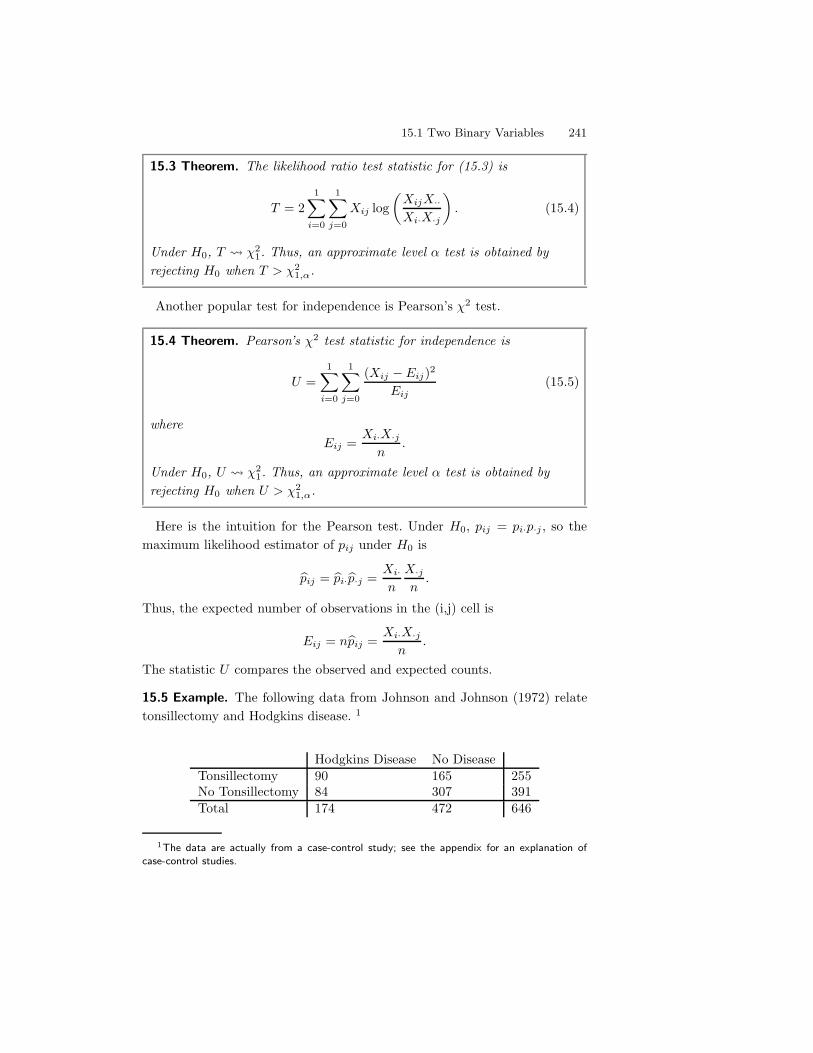
15.1 Two Binary Variables 241
15.3 Theorem. The likelihood ratio test statistic for (15.3) is
T = 21*
i=0
1*
j=0
Xij log-
XijX··
Xi·X·j
.. (15.4)
Under H0, T ! !21. Thus, an approximate level ) test is obtained by
rejecting H0 when T > !21,#.
Another popular test for independence is Pearson’s !2 test.
15.4 Theorem. Pearson’s !2 test statistic for independence is
U =1*
i=0
1*
j=0
(Xij " Eij)2
Eij(15.5)
whereEij =
Xi·X·j
n.
Under H0, U ! !21. Thus, an approximate level ) test is obtained by
rejecting H0 when U > !21,#.
Here is the intuition for the Pearson test. Under H0, pij = pi·p·j , so themaximum likelihood estimator of pij under H0 is
1pij = 1pi·1p·j =Xi·
n
X·j
n.
Thus, the expected number of observations in the (i,j) cell is
Eij = n1pij =Xi·X·j
n.
The statistic U compares the observed and expected counts.
15.5 Example. The following data from Johnson and Johnson (1972) relatetonsillectomy and Hodgkins disease. 1
Hodgkins Disease No DiseaseTonsillectomy 90 165 255No Tonsillectomy 84 307 391Total 174 472 646
1The data are actually from a case-control study; see the appendix for an explanation ofcase-control studies.
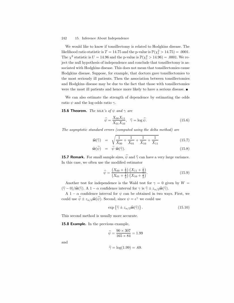
242 15. Inference About Independence
We would like to know if tonsillectomy is related to Hodgkins disease. Thelikelihood ratio statistic is T = 14.75 and the p-value is P(!2
1 > 14.75) = .0001.The !2 statistic is U = 14.96 and the p-value is P(!2
1 > 14.96) = .0001. We re-ject the null hypothesis of independence and conclude that tonsillectomy is as-sociated with Hodgkins disease. This does not mean that tonsillectomies causeHodgkins disease. Suppose, for example, that doctors gave tonsillectomies tothe most seriously ill patients. Then the association between tonsillectomiesand Hodgkins disease may be due to the fact that those with tonsillectomieswere the most ill patients and hence more likely to have a serious disease. !
We can also estimate the strength of dependence by estimating the oddsratio , and the log-odds ratio /.
15.6 Theorem. The mle’s of , and / are
1, =X00X11
X01X10, 1/ = log 1,. (15.6)
The asymptotic standard errors (computed using the delta method) are
1se(1/) =U
1X00
+1
X01+
1X10
+1
X11(15.7)
1se( 1,) = 1, 1se(1/). (15.8)
15.7 Remark. For small sample sizes, 1, and 1/ can have a very large variance.In this case, we often use the modified estimator
1, =;X00 + 1
2
< ;X11 + 1
2
<;X01 + 1
2
< ;X10 + 1
2
< . (15.9)
Another test for independence is the Wald test for / = 0 given by W =(1/ " 0)/1se(1/). A 1" ) confidence interval for / is 1/ ± z#/2 1se(1/).
A 1 " ) confidence interval for , can be obtained in two ways. First, wecould use 1, ± z#/2 1se( 1,). Second, since , = e, we could use
expZ1/ ± z#/2 1se(1/)
[. (15.10)
This second method is usually more accurate.
15.8 Example. In the previous example,
1, =90- 307165- 84
= 1.99
and1/ = log(1.99) = .69.
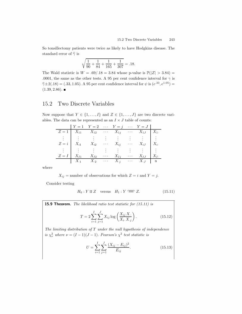
15.2 Two Discrete Variables 243
So tonsillectomy patients were twice as likely to have Hodgkins disease. Thestandard error of 1/ is
U190
+184
+1
165+
1307
= .18.
The Wald statistic is W = .69/.18 = 3.84 whose p-value is P(|Z| > 3.84) =.0001, the same as the other tests. A 95 per cent confidence interval for / is1/±2(.18) = (.33, 1.05). A 95 per cent confidence interval for , is (e.33, e1.05) =(1.39, 2.86). !
15.2 Two Discrete Variables
Now suppose that Y $ {1, . . . , I} and Z $ {1, . . . , J} are two discrete vari-ables. The data can be represented as an I - J table of counts:
Y = 1 Y = 2 · · · Y = j · · · Y = JZ = 1 X11 X12 · · · X1j · · · X1J X1·
......
......
......
......
Z = i Xi1 Xi2 · · · Xij · · · XiJ Xi·...
......
......
......
...Z = I XI1 XI2 · · · XIj · · · XIJ XI·
X·1 X·2 · · · X·j · · · X·J n
where
Xij = number of observations for which Z = i and Y = j.
Consider testing
H0 : Y ! Z versus H1 : Y !""""# Z. (15.11)
15.9 Theorem. The likelihood ratio test statistic for (15.11) is
T = 2I*
i=1
J*
j=1
Xij log-
Xij X··
Xi· X·j
.. (15.12)
The limiting distribution of T under the null hypothesis of independenceis !2
$ where * = (I " 1)(J " 1). Pearson’s !2 test statistic is
U =I*
i=1
J*
j=1
(Xij " Eij)2
Eij. (15.13)
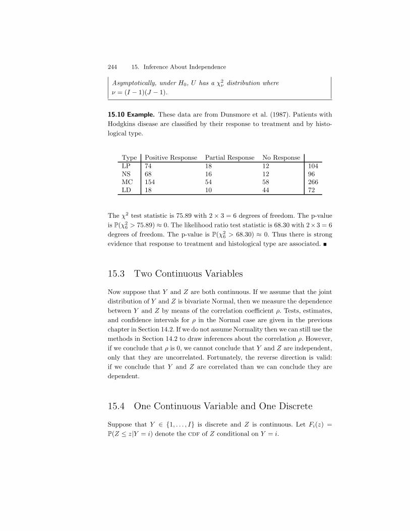
244 15. Inference About Independence
Asymptotically, under H0, U has a !2$ distribution where
* = (I " 1)(J " 1).
15.10 Example. These data are from Dunsmore et al. (1987). Patients withHodgkins disease are classified by their response to treatment and by histo-logical type.
Type Positive Response Partial Response No ResponseLP 74 18 12 104NS 68 16 12 96MC 154 54 58 266LD 18 10 44 72
The !2 test statistic is 75.89 with 2- 3 = 6 degrees of freedom. The p-valueis P(!2
6 > 75.89) . 0. The likelihood ratio test statistic is 68.30 with 2-3 = 6degrees of freedom. The p-value is P(!2
6 > 68.30) . 0. Thus there is strongevidence that response to treatment and histological type are associated. !
15.3 Two Continuous Variables
Now suppose that Y and Z are both continuous. If we assume that the jointdistribution of Y and Z is bivariate Normal, then we measure the dependencebetween Y and Z by means of the correlation coe#cient +. Tests, estimates,and confidence intervals for + in the Normal case are given in the previouschapter in Section 14.2. If we do not assume Normality then we can still use themethods in Section 14.2 to draw inferences about the correlation +. However,if we conclude that + is 0, we cannot conclude that Y and Z are independent,only that they are uncorrelated. Fortunately, the reverse direction is valid:if we conclude that Y and Z are correlated than we can conclude they aredependent.
15.4 One Continuous Variable and One Discrete
Suppose that Y $ {1, . . . , I} is discrete and Z is continuous. Let Fi(z) =P(Z , z|Y = i) denote the cdf of Z conditional on Y = i.
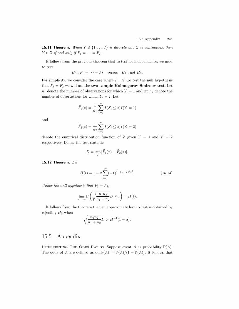
15.5 Appendix 245
15.11 Theorem. When Y $ {1, . . . , I} is discrete and Z is continuous, thenY ! Z if and only if F1 = · · · = FI .
It follows from the previous theorem that to test for independence, we needto test
H0 : F1 = · · · = FI versus H1 : not H0.
For simplicity, we consider the case where I = 2. To test the null hypothesisthat F1 = F2 we will use the two sample Kolmogorov-Smirnov test. Letn1 denote the number of observations for which Yi = 1 and let n2 denote thenumber of observations for which Yi = 2. Let
1F1(z) =1n1
n*
i=1
I(Zi , z)I(Yi = 1)
and1F2(z) =
1n2
n*
i=1
I(Zi , z)I(Yi = 2)
denote the empirical distribution function of Z given Y = 1 and Y = 2respectively. Define the test statistic
D = supx
| 1F1(x) " 1F2(x)|.
15.12 Theorem. Let
H(t) = 1" 2!*
j=1
("1)j$1e$2j2t2 . (15.14)
Under the null hypothesis that F1 = F2,
limn"!
P-U
n1n2
n1 + n2D , t
.= H(t).
It follows from the theorem that an approximate level ) test is obtained byrejecting H0 when U
n1n2
n1 + n2D > H$1(1" )).
15.5 Appendix
Interpreting The Odds Ratios. Suppose event A as probability P(A).The odds of A are defined as odds(A) = P(A)/(1 " P(A)). It follows that
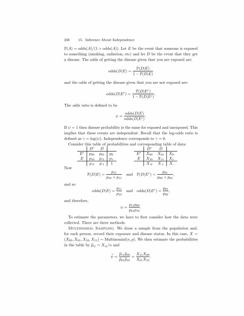
246 15. Inference About Independence
P(A) = odds(A)/(1 + odds(A)). Let E be the event that someone is exposedto something (smoking, radiation, etc) and let D be the event that they geta disease. The odds of getting the disease given that you are exposed are:
odds(D|E) =P(D|E)
1" P(D|E)
and the odds of getting the disease given that you are not exposed are:
odds(D|Ec) =P(D|Ec)
1" P(D|Ec).
The odds ratio is defined to be
, =odds(D|E)odds(D|Ec)
.
If , = 1 then disease probability is the same for exposed and unexposed. Thisimplies that these events are independent. Recall that the log-odds ratio isdefined as / = log(,). Independence corresponds to / = 0.
Consider this table of probabilities and corresponding table of data:Dc D
Ec p00 p01 p0·E p10 p11 p1·
p·0 p·1 1
Dc DEc X00 X01 X0·E X10 X11 X1·
X·0 X·1 X··Now
P(D|E) =p11
p10 + p11and P(D|Ec) =
p01
p00 + p01,
and so
odds(D|E) =p11
p10and odds(D|Ec) =
p01
p00,
and therefore,
, =p11p00
p01p10.
To estimate the parameters, we have to first consider how the data werecollected. There are three methods.
Multinomial Sampling. We draw a sample from the population and,for each person, record their exposure and disease status. In this case, X =(X00, X01, X10, X11) !Multinomial(n, p). We then estimate the probabilitiesin the table by 1pij = Xij/n and
1, =1p111p00
1p011p10=
X11X00
X01X10.
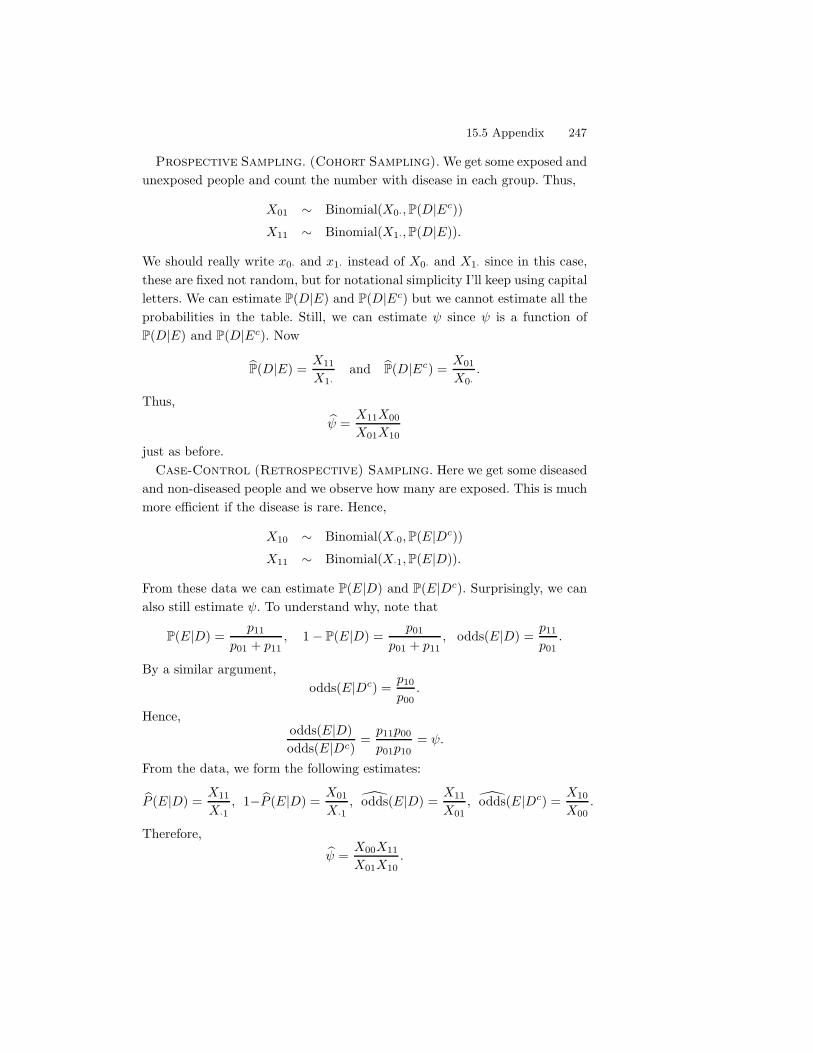
15.5 Appendix 247
Prospective Sampling. (Cohort Sampling). We get some exposed andunexposed people and count the number with disease in each group. Thus,
X01 ! Binomial(X0·, P(D|Ec))
X11 ! Binomial(X1·, P(D|E)).
We should really write x0· and x1· instead of X0· and X1· since in this case,these are fixed not random, but for notational simplicity I’ll keep using capitalletters. We can estimate P(D|E) and P(D|Ec) but we cannot estimate all theprobabilities in the table. Still, we can estimate , since , is a function ofP(D|E) and P(D|Ec). Now
1P(D|E) =X11
X1·and 1P(D|Ec) =
X01
X0·.
Thus,1, =
X11X00
X01X10
just as before.Case-Control (Retrospective) Sampling. Here we get some diseased
and non-diseased people and we observe how many are exposed. This is muchmore e#cient if the disease is rare. Hence,
X10 ! Binomial(X·0, P(E|Dc))
X11 ! Binomial(X·1, P(E|D)).
From these data we can estimate P(E|D) and P(E|Dc). Surprisingly, we canalso still estimate ,. To understand why, note that
P(E|D) =p11
p01 + p11, 1" P(E|D) =
p01
p01 + p11, odds(E|D) =
p11
p01.
By a similar argument,odds(E|Dc) =
p10
p00.
Hence,odds(E|D)odds(E|Dc)
=p11p00
p01p10= ,.
From the data, we form the following estimates:
1P (E|D) =X11
X·1, 1" 1P (E|D) =
X01
X·1, !odds(E|D) =
X11
X01, !odds(E|Dc) =
X10
X00.
Therefore,1, =
X00X11
X01X10.
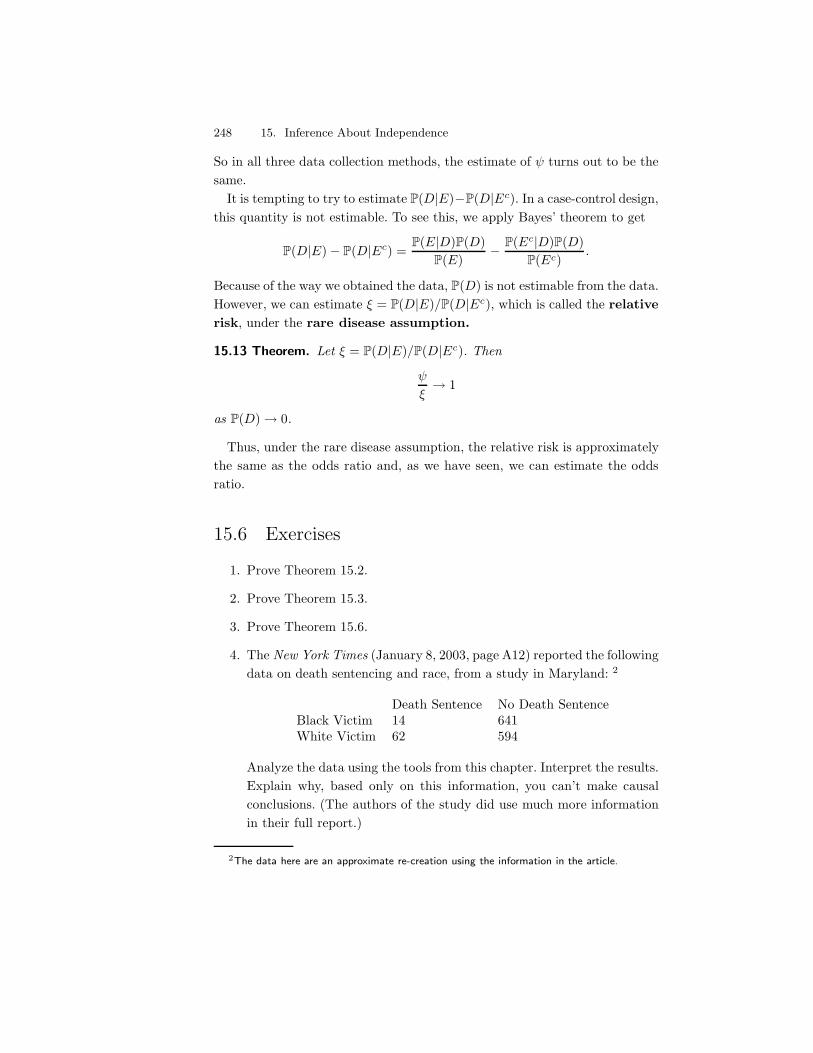
248 15. Inference About Independence
So in all three data collection methods, the estimate of , turns out to be thesame.
It is tempting to try to estimate P(D|E)"P(D|Ec). In a case-control design,this quantity is not estimable. To see this, we apply Bayes’ theorem to get
P(D|E)" P(D|Ec) =P(E|D)P(D)
P(E)" P(Ec|D)P(D)
P(Ec).
Because of the way we obtained the data, P(D) is not estimable from the data.However, we can estimate . = P(D|E)/P(D|Ec), which is called the relativerisk, under the rare disease assumption.
15.13 Theorem. Let . = P(D|E)/P(D|Ec). Then
,
.) 1
as P(D)) 0.
Thus, under the rare disease assumption, the relative risk is approximatelythe same as the odds ratio and, as we have seen, we can estimate the oddsratio.
15.6 Exercises
1. Prove Theorem 15.2.
2. Prove Theorem 15.3.
3. Prove Theorem 15.6.
4. The New York Times (January 8, 2003, page A12) reported the followingdata on death sentencing and race, from a study in Maryland: 2
Death Sentence No Death SentenceBlack Victim 14 641White Victim 62 594
Analyze the data using the tools from this chapter. Interpret the results.Explain why, based only on this information, you can’t make causalconclusions. (The authors of the study did use much more informationin their full report.)
2The data here are an approximate re-creation using the information in the article.

15.6 Exercises 249
5. Analyze the data on the variables Age and Financial Status from:
http://lib.stat.cmu.edu/DASL/Datafiles/montanadat.html
6. Estimate the correlation between temperature and latitude using thedata from
http://lib.stat.cmu.edu/DASL/Datafiles/USTemperatures.html
Use the correlation coe#cient. Provide estimates, tests, and confidenceintervals.
7. Test whether calcium intake and drop in blood pressure are associated.Use the data in
http://lib.stat.cmu.edu/DASL/Datafiles/Calcium.html

This is page 250Printer: Opaque this
This is page 251Printer: Opaque this
16Causal Inference
Roughly speaking, the statement “X causes Y ” means that changing thevalue of X will change the distribution of Y . When X causes Y , X and Y
will be associated but the reverse is not, in general, true. Association does notnecessarily imply causation. We will consider two frameworks for discussingcausation. The first uses counterfactual random variables. The second, pre-sented in the next chapter, uses directed acyclic graphs.
16.1 The Counterfactual Model
Suppose that X is a binary treatment variable where X = 1 means “treated”and X = 0 means “not treated.” We are using the word “treatment” in avery broad sense. Treatment might refer to a medication or something likesmoking. An alternative to “treated/not treated” is “exposed/not exposed”but we shall use the former.
Let Y be some outcome variable such as presence or absence of disease.To distinguish the statement “X is associated Y ” from the statement “X
causes Y ” we need to enrich our probabilistic vocabulary. Specifically, we willdecompose the response Y into a more fine-grained object.
We introduce two new random variables (C0, C1), called potential out-comes with the following interpretation: C0 is the outcome if the subject is
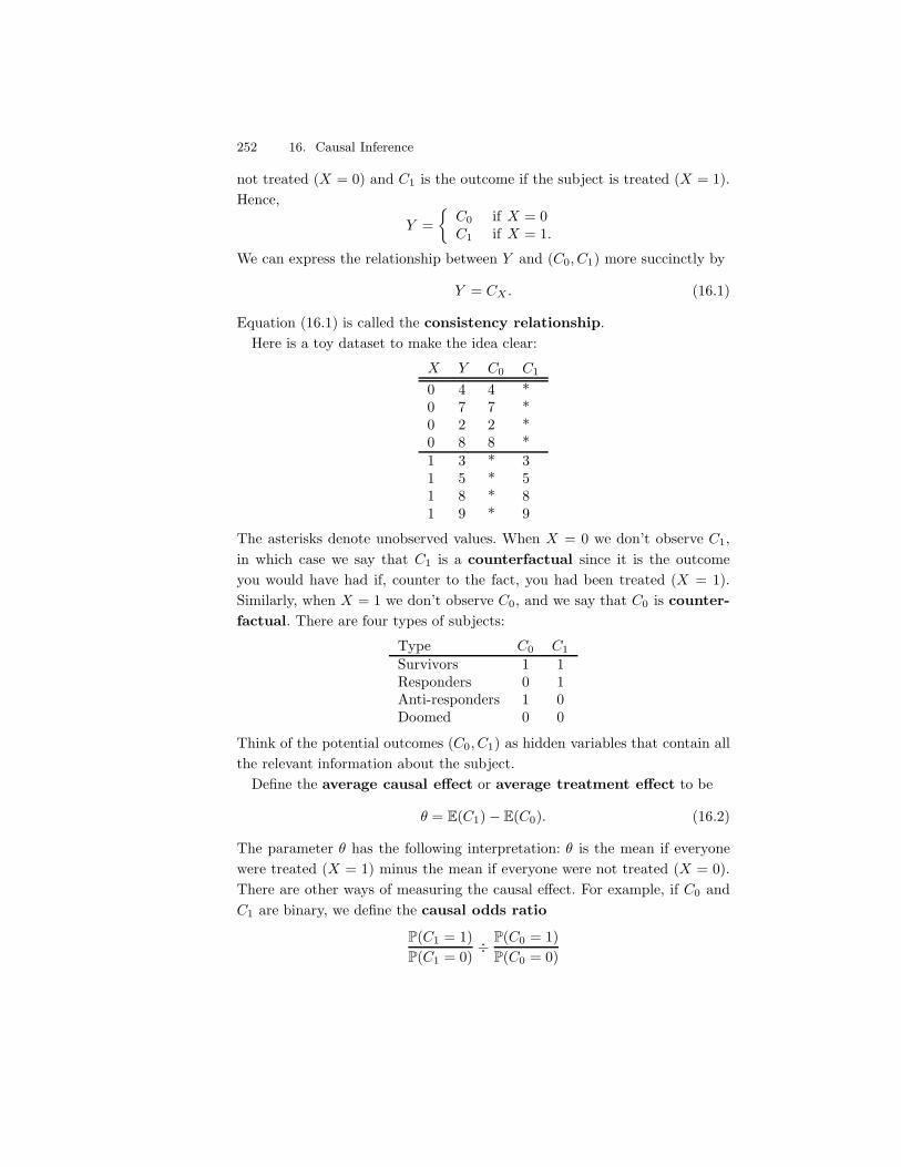
252 16. Causal Inference
not treated (X = 0) and C1 is the outcome if the subject is treated (X = 1).Hence,
Y ='
C0 if X = 0C1 if X = 1.
We can express the relationship between Y and (C0, C1) more succinctly by
Y = CX . (16.1)
Equation (16.1) is called the consistency relationship.Here is a toy dataset to make the idea clear:
X Y C0 C1
0 4 4 *0 7 7 *0 2 2 *0 8 8 *1 3 * 31 5 * 51 8 * 81 9 * 9
The asterisks denote unobserved values. When X = 0 we don’t observe C1,in which case we say that C1 is a counterfactual since it is the outcomeyou would have had if, counter to the fact, you had been treated (X = 1).Similarly, when X = 1 we don’t observe C0, and we say that C0 is counter-factual. There are four types of subjects:
Type C0 C1
Survivors 1 1Responders 0 1Anti-responders 1 0Doomed 0 0
Think of the potential outcomes (C0, C1) as hidden variables that contain allthe relevant information about the subject.
Define the average causal e"ect or average treatment e"ect to be
0 = E(C1)" E(C0). (16.2)
The parameter 0 has the following interpretation: 0 is the mean if everyonewere treated (X = 1) minus the mean if everyone were not treated (X = 0).There are other ways of measuring the causal e!ect. For example, if C0 andC1 are binary, we define the causal odds ratio
P(C1 = 1)P(C1 = 0)
÷ P(C0 = 1)P(C0 = 0)
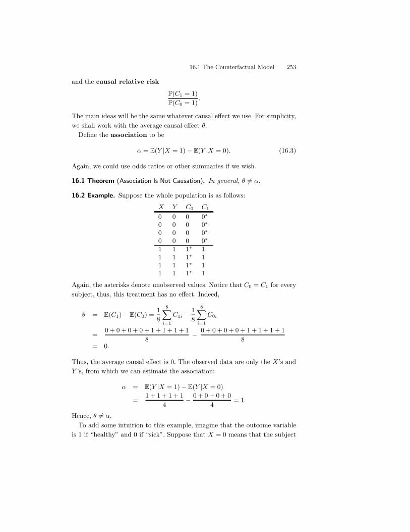
16.1 The Counterfactual Model 253
and the causal relative risk
P(C1 = 1)P(C0 = 1)
.
The main ideas will be the same whatever causal e!ect we use. For simplicity,we shall work with the average causal e!ect 0.
Define the association to be
) = E(Y |X = 1)" E(Y |X = 0). (16.3)
Again, we could use odds ratios or other summaries if we wish.
16.1 Theorem (Association Is Not Causation). In general, 0 (= ).
16.2 Example. Suppose the whole population is as follows:
X Y C0 C1
0 0 0 0*0 0 0 0*0 0 0 0*0 0 0 0*
1 1 1* 11 1 1* 11 1 1* 11 1 1* 1
Again, the asterisks denote unobserved values. Notice that C0 = C1 for everysubject, thus, this treatment has no e!ect. Indeed,
0 = E(C1)" E(C0) =18
8*
i=1
C1i "18
8*
i=1
C0i
=0 + 0 + 0 + 0 + 1 + 1 + 1 + 1
8" 0 + 0 + 0 + 0 + 1 + 1 + 1 + 1
8= 0.
Thus, the average causal e!ect is 0. The observed data are only the X ’s andY ’s, from which we can estimate the association:
) = E(Y |X = 1)" E(Y |X = 0)
=1 + 1 + 1 + 1
4" 0 + 0 + 0 + 0
4= 1.
Hence, 0 (= ).To add some intuition to this example, imagine that the outcome variable
is 1 if “healthy” and 0 if “sick”. Suppose that X = 0 means that the subject
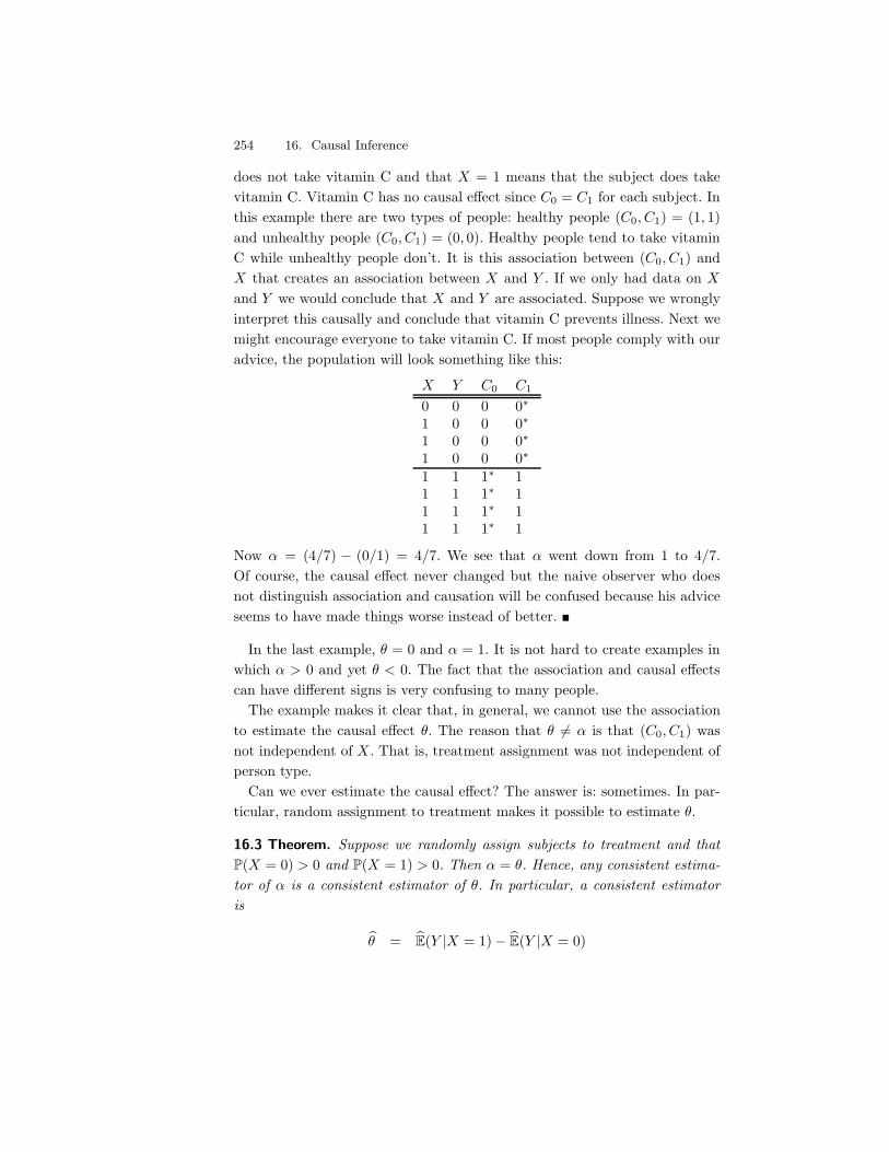
254 16. Causal Inference
does not take vitamin C and that X = 1 means that the subject does takevitamin C. Vitamin C has no causal e!ect since C0 = C1 for each subject. Inthis example there are two types of people: healthy people (C0, C1) = (1, 1)and unhealthy people (C0, C1) = (0, 0). Healthy people tend to take vitaminC while unhealthy people don’t. It is this association between (C0, C1) andX that creates an association between X and Y . If we only had data on X
and Y we would conclude that X and Y are associated. Suppose we wronglyinterpret this causally and conclude that vitamin C prevents illness. Next wemight encourage everyone to take vitamin C. If most people comply with ouradvice, the population will look something like this:
X Y C0 C1
0 0 0 0*1 0 0 0*1 0 0 0*1 0 0 0*
1 1 1* 11 1 1* 11 1 1* 11 1 1* 1
Now ) = (4/7) " (0/1) = 4/7. We see that ) went down from 1 to 4/7.Of course, the causal e!ect never changed but the naive observer who doesnot distinguish association and causation will be confused because his adviceseems to have made things worse instead of better. !
In the last example, 0 = 0 and ) = 1. It is not hard to create examples inwhich ) > 0 and yet 0 < 0. The fact that the association and causal e!ectscan have di!erent signs is very confusing to many people.
The example makes it clear that, in general, we cannot use the associationto estimate the causal e!ect 0. The reason that 0 (= ) is that (C0, C1) wasnot independent of X . That is, treatment assignment was not independent ofperson type.
Can we ever estimate the causal e!ect? The answer is: sometimes. In par-ticular, random assignment to treatment makes it possible to estimate 0.
16.3 Theorem. Suppose we randomly assign subjects to treatment and thatP(X = 0) > 0 and P(X = 1) > 0. Then ) = 0. Hence, any consistent estima-tor of ) is a consistent estimator of 0. In particular, a consistent estimatoris
10 = 1E(Y |X = 1)" 1E(Y |X = 0)
16.2 Beyond Binary Treatments 255
= Y 1 " Y 0
is a consistent estimator of 0, where
Y 1 =1n1
n*
i=1
YiXi, Y 0 =1n0
n*
i=1
Yi(1"Xi),
n1 =0n
i=1 Xi, and n0 =0n
i=1(1 "Xi).
Proof. Since X is randomly assigned, X is independent of (C0, C1). Hence,
0 = E(C1)" E(C0)
= E(C1|X = 1)" E(C0|X = 0) since X ! (C0, C1)
= E(Y |X = 1)" E(Y |X = 0) since Y = CX
= ).
The consistency follows from the law of large numbers. !
If Z is a covariate, we define the conditional causal e"ect by
0z = E(C1|Z = z)" E(C0|Z = z).
For example, if Z denotes gender with values Z = 0 (women) and Z = 1(men), then 00 is the causal e!ect among women and 01 is the causal e!ectamong men. In a randomized experiment, 0z = E(Y |X = 1, Z = z)"E(Y |X =0, Z = z) and we can estimate the conditional causal e!ect using appropriatesample averages.
Summary of the Counterfactual Model
Random variables: (C0, C1, X, Y ).Consistency relationship: Y = CX .Causal E!ect: 0 = E(C1)" E(C0).Association: ) = E(Y |X = 1)" E(Y |X = 0).Random assignment =+ (C0, C1) ! X =+ 0 = ).
16.2 Beyond Binary Treatments
Let us now generalize beyond the binary case. Suppose that X $ X . Forexample, X could be the dose of a drug in which case X $ R. The counterfac-tual vector (C0, C1) now becomes the counterfactual function C(x) where
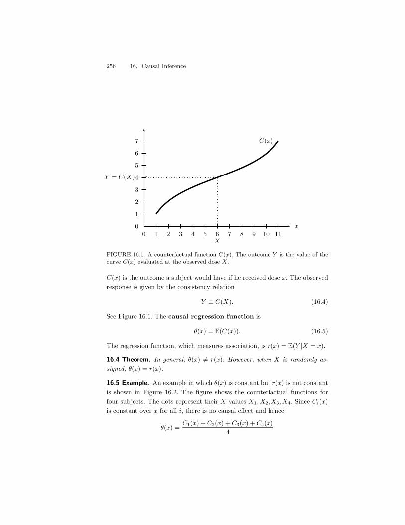
256 16. Causal Inference
0 1 2 3 4 5 6 7 8 9 10 110
1
2
3
4
5
6
7
x
C(x)
X
Y = C(X)
FIGURE 16.1. A counterfactual function C(x). The outcome Y is the value of thecurve C(x) evaluated at the observed dose X.
C(x) is the outcome a subject would have if he received dose x. The observedresponse is given by the consistency relation
Y 0 C(X). (16.4)
See Figure 16.1. The causal regression function is
0(x) = E(C(x)). (16.5)
The regression function, which measures association, is r(x) = E(Y |X = x).
16.4 Theorem. In general, 0(x) (= r(x). However, when X is randomly as-signed, 0(x) = r(x).
16.5 Example. An example in which 0(x) is constant but r(x) is not constantis shown in Figure 16.2. The figure shows the counterfactual functions forfour subjects. The dots represent their X values X1, X2, X3, X4. Since Ci(x)is constant over x for all i, there is no causal e!ect and hence
0(x) =C1(x) + C2(x) + C3(x) + C4(x)
4
16.3 Observational Studies and Confounding 257
is constant. Changing the dose x will not change anyone’s outcome. The fourdots in the lower plot represent the observed data points Y1 = C1(X1), Y2 =C2(X2), Y3 = C3(X3), Y4 = C4(X4). The dotted line represents the regressionr(x) = E(Y |X = x). Although there is no causal e!ect, there is an associationsince the regression curve r(x) is not constant. !
16.3 Observational Studies and Confounding
A study in which treatment (or exposure) is not randomly assigned is called anobservational study. In these studies, subjects select their own value of theexposure X . Many of the health studies you read about in the newspaper arelike this. As we saw, association and causation could in general be quite di!er-ent. This discrepancy occurs in non-randomized studies because the potentialoutcome C is not independent of treatment X . However, suppose we couldfind groupings of subjects such that, within groups, X and {C(x) : x $ X}are independent. This would happen if the subjects are very similar withingroups. For example, suppose we find people who are very similar in age, gen-der, educational background, and ethnic background. Among these people wemight feel it is reasonable to assume that the choice of X is essentially ran-dom. These other variables are called confounding variables.1 If we denotethese other variables collectively as Z, then we can express this idea by sayingthat
{C(x) : x $ X} ! X |Z. (16.6)
Equation (16.6) means that, within groups of Z, the choice of treatment X
does not depend on type, as represented by {C(x) : x $ X}. If (16.6) holdsand we observe Z then we say that there is no unmeasured confounding.
16.6 Theorem. Suppose that (16.6) holds. Then,
0(x) =9
E(Y |X = x, Z = z)dFZ(z)dz. (16.7)
If 1r(x, z) is a consistent estimate of the regression function E(Y |X = x, Z =z), then a consistent estimate of 0(x) is
10(x) =1n
n*
i=1
1r(x, Zi).
1A more precise definition of confounding is given in the next chapter.
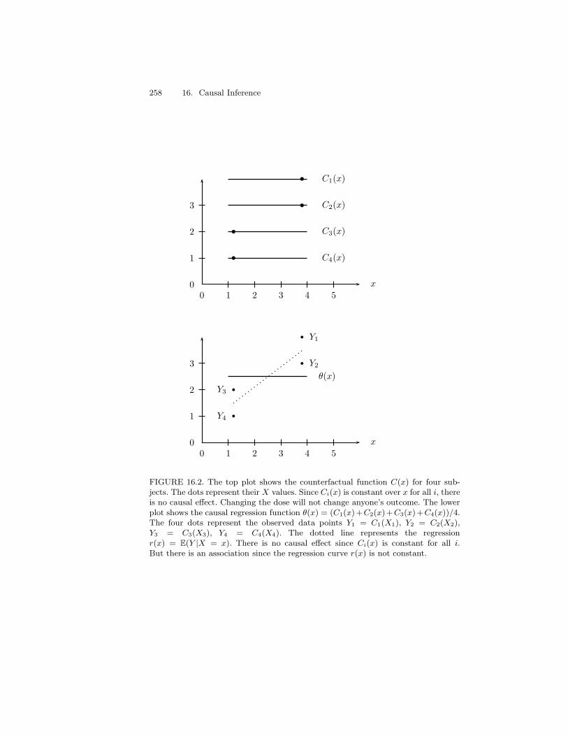
258 16. Causal Inference
0 1 2 3 4 50
1
2
3
C1(x)
C2(x)
C3(x)
C4(x)
x
0 1 2 3 4 50
1
2
30(x)
Y1
Y2
Y3
Y4
x
FIGURE 16.2. The top plot shows the counterfactual function C(x) for four sub-jects. The dots represent their X values. Since Ci(x) is constant over x for all i, thereis no causal e"ect. Changing the dose will not change anyone’s outcome. The lowerplot shows the causal regression function !(x) = (C1(x)+C2(x)+C3(x)+C4(x))/4.The four dots represent the observed data points Y1 = C1(X1), Y2 = C2(X2),Y3 = C3(X3), Y4 = C4(X4). The dotted line represents the regressionr(x) = E(Y |X = x). There is no causal e"ect since Ci(x) is constant for all i.But there is an association since the regression curve r(x) is not constant.
16.4 Simpson’s Paradox 259
In particular, if r(x, z) = (0 + (1x + (2z is linear, then a consistent estimateof 0(x) is
10(x) = 1(0 + 1(1x + 1(2Zn (16.8)
where (1(0, 1(1, 1(2) are the least squares estimators.
16.7 Remark. It is useful to compare equation (16.7) to E(Y |X = x) whichcan be written as E(Y |X = x) =
8E(Y |X = x, Z = z)dFZ|X(z|x).
Epidemiologists call (16.7) the adjusted treatment e"ect. The process ofcomputing adjusted treatment e!ects is called adjusting (or controlling)for confounding. The selection of what confounders Z to measure and con-trol for requires scientific insight. Even after adjusting for confounders, wecannot be sure that there are not other confounding variables that we missed.This is why observational studies must be treated with healthy skepticism.Results from observational studies start to become believable when: (i) theresults are replicated in many studies, (ii) each of the studies controlled forplausible confounding variables, (iii) there is a plausible scientific explanationfor the existence of a causal relationship.
A good example is smoking and cancer. Numerous studies have shown arelationship between smoking and cancer even after adjusting for many con-founding variables. Moreover, in laboratory studies, smoking has been shownto damage lung cells. Finally, a causal link between smoking and cancer hasbeen found in randomized animal studies. It is this collection of evidenceover many years that makes this a convincing case. One single observationalstudy is not, by itself, strong evidence. Remember that when you read thenewspaper.
16.4 Simpson’s Paradox
Simpson’s paradox is a puzzling phenomenon that is discussed in most statis-tics texts. Unfortunately, most explanations are confusing (and in some casesincorrect). The reason is that it is nearly impossible to explain the paradoxwithout using counterfactuals (or directed acyclic graphs).
Let X be a binary treatment variable, Y a binary outcome, and Z a thirdbinary variable such as gender. Suppose the joint distribution of X, Y, Z is
260 16. Causal Inference
Y = 1 Y = 0 Y = 1 Y = 0X = 1 .1500 .2250 .1000 .0250X = 0 .0375 .0875 .2625 .1125
Z = 1 (men) Z = 0 (women)
The marginal distribution for (X, Y ) is
Y = 1 Y = 0X = 1 .25 .25 .50X = 0 .30 .20 .50
.55 .45 1
From these tables we find that,
P(Y = 1|X = 1)" P(Y = 1|X = 0) = "0.1
P(Y = 1|X = 1, Z = 1)" P(Y = 1|X = 0, Z = 1) = 0.1
P(Y = 1|X = 1, Z = 0)" P(Y = 1|X = 0, Z = 0) = 0.1.
To summarize, we seem to have the following information:
Mathematical Statement English Statement?P(Y = 1|X = 1) < P(Y = 1|X = 0) treatment is harmful
P(Y = 1|X = 1, Z = 1) > P(Y = 1|X = 0, Z = 1) treatment is beneficial to menP(Y = 1|X = 1, Z = 0) > P(Y = 1|X = 0, Z = 0) treatment is beneficial to women
Clearly, something is amiss. There can’t be a treatment which is good formen, good for women, but bad overall. This is nonsense. The problem is withthe set of English statements in the table. Our translation from math intoEnglish is specious.
The inequality P(Y = 1|X = 1) < P(Y = 1|X = 0) does notmean that treatment is harmful.
The phrase “treatment is harmful” should be written mathematically asP(C1 = 1) < P(C0 = 1). The phrase “treatment is harmful for men” shouldbe written P(C1 = 1|Z = 1) < P(C0 = 1|Z = 1). The three mathematicalstatements in the table are not at all contradictory. It is only the translationinto English that is wrong.
Let us now show that a real Simpson’s paradox cannot happen, that is,there cannot be a treatment that is beneficial for men and women but harmfuloverall. Suppose that treatment is beneficial for both sexes. Then
P(C1 = 1|Z = z) > P(C0 = 1|Z = z)
16.5 Bibliographic Remarks 261
for all z. It then follows that
P(C1 = 1) =*
z
P(C1 = 1|Z = z)P(Z = z)
>*
z
P(C0 = 1|Z = z)P(Z = z)
= P(C0 = 1).
Hence, P(C1 = 1) > P(C0 = 1), so treatment is beneficial overall. No paradox.
16.5 Bibliographic Remarks
The use of potential outcomes to clarify causation is due mainly to Jerzy Ney-man and Donald Rubin. Later developments are due to Jamie Robins, PaulRosenbaum, and others. A parallel development took place in econometricsby various people including James Heckman and Charles Manski. Texts oncausation include Pearl (2000), Rosenbaum (2002), Spirtes et al. (2000), andvan der Laan and Robins (2003).
16.6 Exercises
1. Create an example like Example 16.2 in which ) > 0 and 0 < 0.
2. Prove Theorem 16.4.
3. Suppose you are given data (X1, Y1), . . . , (Xn, Yn) from an observationalstudy, where Xi $ {0, 1} and Yi $ {0, 1}. Although it is not possibleto estimate the causal e!ect 0, it is possible to put bounds on 0. Findupper and lower bounds on 0 that can be consistently estimated fromthe data. Show that the bounds have width 1.
Hint: Note that E(C1) = E(C1|X = 1)P(X = 1) + E(C1|X = 0)P(X =0).
4. Suppose that X $ R and that, for each subject i, Ci(x) = (1ix. Eachsubject has their own slope (1i. Construct a joint distribution on ((1, X)such that P((1 > 0) = 1 but E(Y |X = x) is a decreasing function of x,where Y = C(X). Interpret.
5. Let X $ {0, 1} be a binary treatment variable and let (C0, C1) denotethe corresponding potential outcomes. Let Y = CX denote the observed

262 16. Causal Inference
response. Let F0 and F1 be the cumulative distribution functions forC0 and C1. Assume that F0 and F1 are both continuous and strictlyincreasing. Let 0 = m1"m0 where m0 = F$1
0 (1/2) is the median of C0
and m1 = F$11 (1/2) is the median of C1. Suppose that the treatment X
is assigned randomly. Find an expression for 0 involving only the jointdistribution of X and Y .
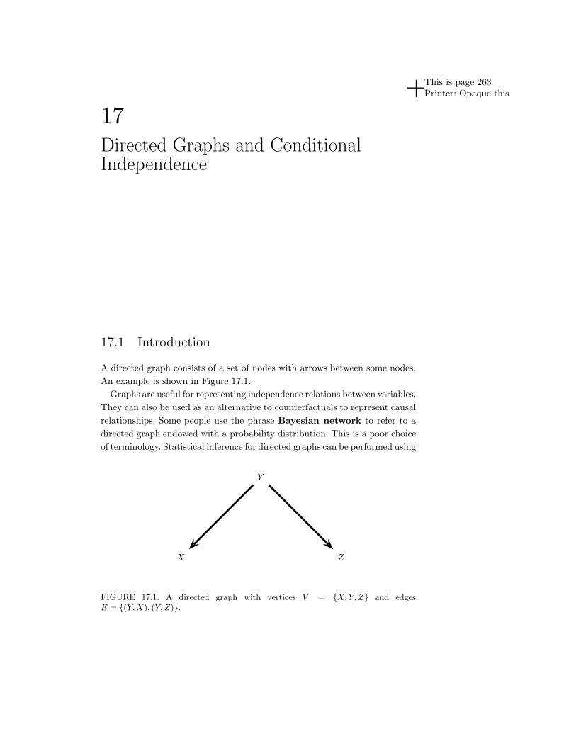
This is page 263Printer: Opaque this
17Directed Graphs and ConditionalIndependence
17.1 Introduction
A directed graph consists of a set of nodes with arrows between some nodes.An example is shown in Figure 17.1.
Graphs are useful for representing independence relations between variables.They can also be used as an alternative to counterfactuals to represent causalrelationships. Some people use the phrase Bayesian network to refer to adirected graph endowed with a probability distribution. This is a poor choiceof terminology. Statistical inference for directed graphs can be performed using
Y
X Z
FIGURE 17.1. A directed graph with vertices V = {X, Y, Z} and edgesE = {(Y, X), (Y, Z)}.
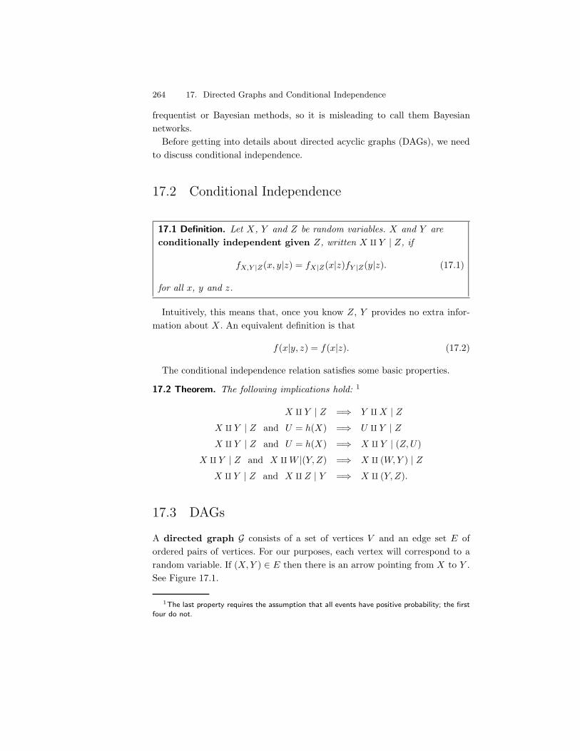
264 17. Directed Graphs and Conditional Independence
frequentist or Bayesian methods, so it is misleading to call them Bayesiannetworks.
Before getting into details about directed acyclic graphs (DAGs), we needto discuss conditional independence.
17.2 Conditional Independence
17.1 Definition. Let X, Y and Z be random variables. X and Y areconditionally independent given Z, written X ! Y | Z, if
fX,Y |Z(x, y|z) = fX|Z(x|z)fY |Z(y|z). (17.1)
for all x, y and z.
Intuitively, this means that, once you know Z, Y provides no extra infor-mation about X . An equivalent definition is that
f(x|y, z) = f(x|z). (17.2)
The conditional independence relation satisfies some basic properties.
17.2 Theorem. The following implications hold: 1
X ! Y | Z =+ Y ! X | Z
X ! Y | Z and U = h(X) =+ U ! Y | Z
X ! Y | Z and U = h(X) =+ X ! Y | (Z, U)
X ! Y | Z and X ! W |(Y, Z) =+ X ! (W, Y ) | Z
X ! Y | Z and X ! Z | Y =+ X ! (Y, Z).
17.3 DAGs
A directed graph G consists of a set of vertices V and an edge set E ofordered pairs of vertices. For our purposes, each vertex will correspond to arandom variable. If (X, Y ) $ E then there is an arrow pointing from X to Y .See Figure 17.1.
1The last property requires the assumption that all events have positive probability; the firstfour do not.
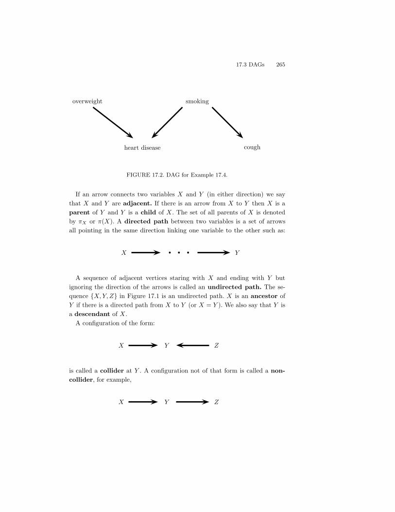
17.3 DAGs 265
heart disease cough
overweight smoking
FIGURE 17.2. DAG for Example 17.4.
If an arrow connects two variables X and Y (in either direction) we saythat X and Y are adjacent. If there is an arrow from X to Y then X is aparent of Y and Y is a child of X . The set of all parents of X is denotedby &X or &(X). A directed path between two variables is a set of arrowsall pointing in the same direction linking one variable to the other such as:
X Y
A sequence of adjacent vertices staring with X and ending with Y butignoring the direction of the arrows is called an undirected path. The se-quence {X, Y, Z} in Figure 17.1 is an undirected path. X is an ancestor ofY if there is a directed path from X to Y (or X = Y ). We also say that Y isa descendant of X .
A configuration of the form:
X Y Z
is called a collider at Y . A configuration not of that form is called a non-collider, for example,
X Y Z
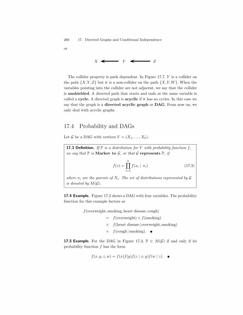
266 17. Directed Graphs and Conditional Independence
or
X Y Z
The collider property is path dependent. In Figure 17.7, Y is a collider onthe path {X, Y, Z} but it is a non-collider on the path {X, Y, W}. When thevariables pointing into the collider are not adjacent, we say that the collideris unshielded. A directed path that starts and ends at the same variable iscalled a cycle. A directed graph is acyclic if it has no cycles. In this case wesay that the graph is a directed acyclic graph or DAG. From now on, weonly deal with acyclic graphs.
17.4 Probability and DAGs
Let G be a DAG with vertices V = (X1, . . . , Xk).
17.3 Definition. If P is a distribution for V with probability function f ,we say that P is Markov to G, or that G represents P, if
f(v) =k/
i=1
f(xi | &i) (17.3)
where &i are the parents of Xi. The set of distributions represented by Gis denoted by M(G).
17.4 Example. Figure 17.2 shows a DAG with four variables. The probabilityfunction for this example factors as
f(overweight, smoking, heart disease, cough)
= f(overweight)- f(smoking)
- f(heart disease | overweight, smoking)
- f(cough | smoking). !
17.5 Example. For the DAG in Figure 17.3, P $ M(G) if and only if itsprobability function f has the form
f(x, y, z, w) = f(x)f(y)f(z | x, y)f(w | z). !
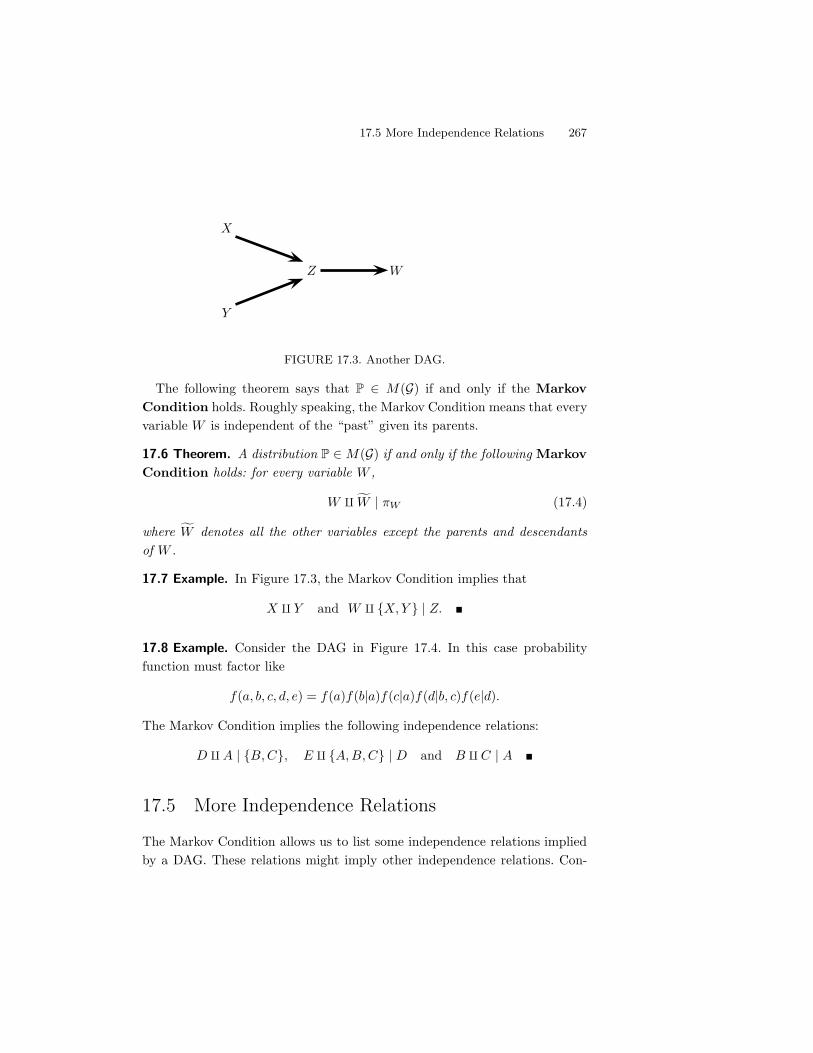
17.5 More Independence Relations 267
Y
X
Z W
FIGURE 17.3. Another DAG.
The following theorem says that P $ M(G) if and only if the MarkovCondition holds. Roughly speaking, the Markov Condition means that everyvariable W is independent of the “past” given its parents.
17.6 Theorem. A distribution P $M(G) if and only if the following MarkovCondition holds: for every variable W ,
W !dW | &W (17.4)
where dW denotes all the other variables except the parents and descendantsof W .
17.7 Example. In Figure 17.3, the Markov Condition implies that
X ! Y and W ! {X, Y } | Z. !
17.8 Example. Consider the DAG in Figure 17.4. In this case probabilityfunction must factor like
f(a, b, c, d, e) = f(a)f(b|a)f(c|a)f(d|b, c)f(e|d).
The Markov Condition implies the following independence relations:
D ! A | {B, C}, E ! {A, B, C} | D and B ! C | A !
17.5 More Independence Relations
The Markov Condition allows us to list some independence relations impliedby a DAG. These relations might imply other independence relations. Con-
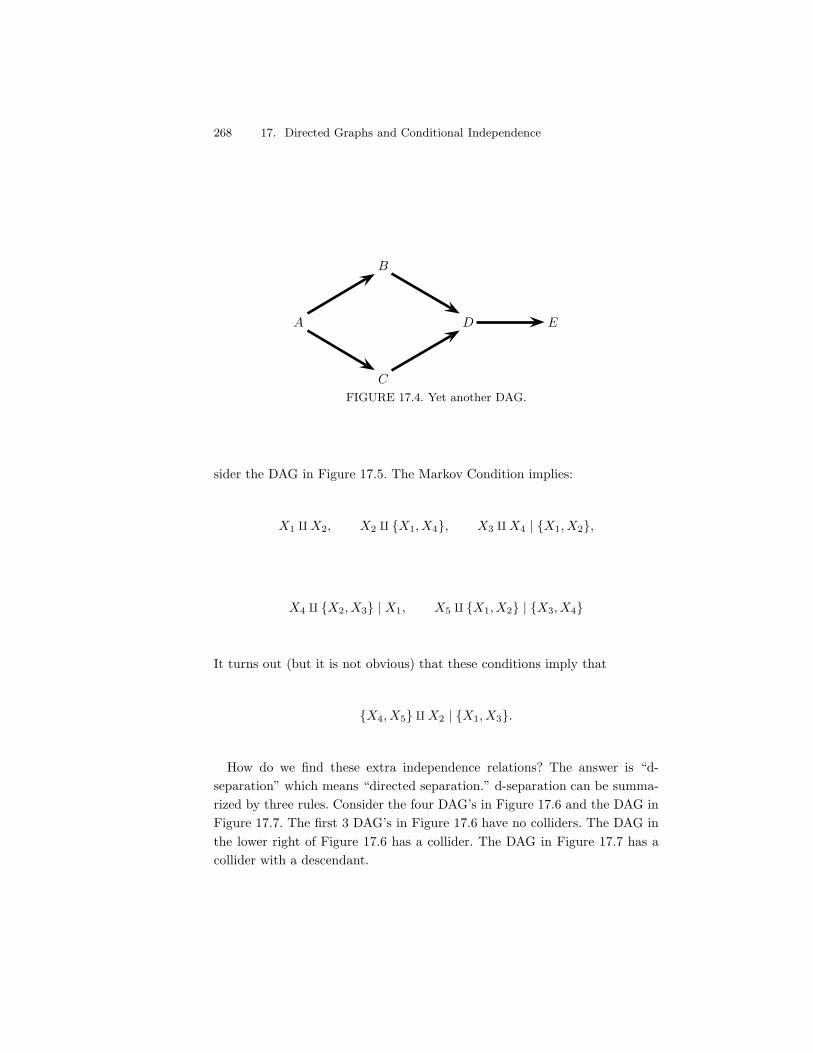
268 17. Directed Graphs and Conditional Independence
A
C
B
D E
FIGURE 17.4. Yet another DAG.
sider the DAG in Figure 17.5. The Markov Condition implies:
X1 ! X2, X2 ! {X1, X4}, X3 ! X4 | {X1, X2},
X4 ! {X2, X3} | X1, X5 ! {X1, X2} | {X3, X4}
It turns out (but it is not obvious) that these conditions imply that
{X4, X5} ! X2 | {X1, X3}.
How do we find these extra independence relations? The answer is “d-separation” which means “directed separation.” d-separation can be summa-rized by three rules. Consider the four DAG’s in Figure 17.6 and the DAG inFigure 17.7. The first 3 DAG’s in Figure 17.6 have no colliders. The DAG inthe lower right of Figure 17.6 has a collider. The DAG in Figure 17.7 has acollider with a descendant.
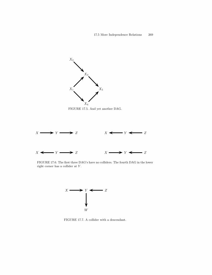
17.5 More Independence Relations 269
X1
X2
X3
X4
X5
FIGURE 17.5. And yet another DAG.
X Y Z X Y Z
X Y Z X Y Z
FIGURE 17.6. The first three DAG’s have no colliders. The fourth DAG in the lowerright corner has a collider at Y .
X Y Z
W
FIGURE 17.7. A collider with a descendant.
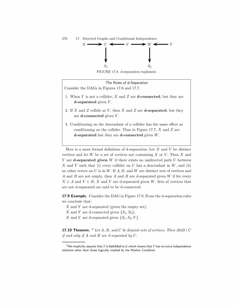
270 17. Directed Graphs and Conditional Independence
X U V W Y
S1 S2
FIGURE 17.8. d-separation explained.
The Rules of d-Separation
Consider the DAGs in Figures 17.6 and 17.7.
1. When Y is not a collider, X and Z are d-connected, but they ared-separated given Y .
2. If X and Z collide at Y , then X and Z are d-separated, but theyare d-connected given Y .
3. Conditioning on the descendant of a collider has the same e!ect asconditioning on the collider. Thus in Figure 17.7, X and Z ared-separated but they are d-connected given W .
Here is a more formal definition of d-separation. Let X and Y be distinctvertices and let W be a set of vertices not containing X or Y . Then X andY are d-separated given W if there exists no undirected path U betweenX and Y such that (i) every collider on U has a descendant in W , and (ii)no other vertex on U is in W . If A, B, and W are distinct sets of vertices andA and B are not empty, then A and B are d-separated given W if for everyX $ A and Y $ B, X and Y are d-separated given W . Sets of vertices thatare not d-separated are said to be d-connected.
17.9 Example. Consider the DAG in Figure 17.8. From the d-separation ruleswe conclude that:
X and Y are d-separated (given the empty set);X and Y are d-connected given {S1, S2};X and Y are d-separated given {S1, S2, V }.
17.10 Theorem. 2 Let A, B, and C be disjoint sets of vertices. Then A!B | C
if and only if A and B are d-separated by C.
2We implicitly assume that P is faithful to G which means that P has no extra independencerelations other than those logically implied by the Markov Condition.
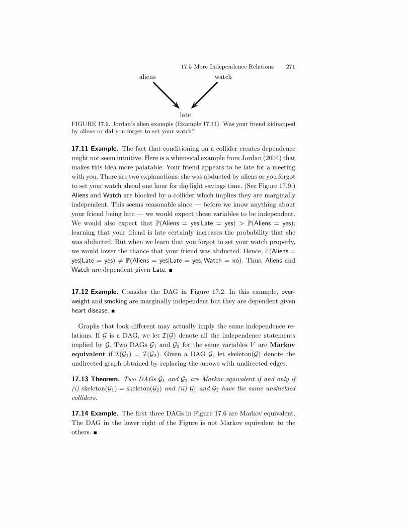
17.5 More Independence Relations 271
late
aliens watch
FIGURE 17.9. Jordan’s alien example (Example 17.11). Was your friend kidnappedby aliens or did you forget to set your watch?
17.11 Example. The fact that conditioning on a collider creates dependencemight not seem intuitive. Here is a whimsical example from Jordan (2004) thatmakes this idea more palatable. Your friend appears to be late for a meetingwith you. There are two explanations: she was abducted by aliens or you forgotto set your watch ahead one hour for daylight savings time. (See Figure 17.9.)Aliens and Watch are blocked by a collider which implies they are marginallyindependent. This seems reasonable since — before we know anything aboutyour friend being late — we would expect these variables to be independent.We would also expect that P(Aliens = yes|Late = yes) > P(Aliens = yes);learning that your friend is late certainly increases the probability that shewas abducted. But when we learn that you forgot to set your watch properly,we would lower the chance that your friend was abducted. Hence, P(Aliens =yes|Late = yes) (= P(Aliens = yes|Late = yes, Watch = no). Thus, Aliens andWatch are dependent given Late. !
17.12 Example. Consider the DAG in Figure 17.2. In this example, over-
weight and smoking are marginally independent but they are dependent givenheart disease. !
Graphs that look di!erent may actually imply the same independence re-lations. If G is a DAG, we let I(G) denote all the independence statementsimplied by G. Two DAGs G1 and G2 for the same variables V are Markovequivalent if I(G1) = I(G2). Given a DAG G, let skeleton(G) denote theundirected graph obtained by replacing the arrows with undirected edges.
17.13 Theorem. Two DAGs G1 and G2 are Markov equivalent if and only if(i) skeleton(G1) = skeleton(G2) and (ii) G1 and G2 have the same unshieldedcolliders.
17.14 Example. The first three DAGs in Figure 17.6 are Markov equivalent.The DAG in the lower right of the Figure is not Markov equivalent to theothers. !
272 17. Directed Graphs and Conditional Independence
17.6 Estimation for DAGs
Two estimation questions arise in the context of DAGs. First, given a DAGG and data V1, . . . , Vn from a distribution f consistent with G, how do weestimate f? Second, given data V1, . . . , Vn how do we estimate G? The firstquestion is pure estimation while the second involves model selection. Theseare very involved topics and are beyond the scope of this book. We will justbriefly mention the main ideas.
Typically, one uses some parametric model f(x|&x; 0x) for each conditionaldensity. The likelihood function is then
L(0) =n/
i=1
f(Vi; 0) =n/
i=1
m/
j=1
f(Xij |&j ; 0j),
where Xij is the value of Xj for the ith data point and 0j are the parameters forthe jth conditional density. We can then estimate the parameters by maximumlikelihood.
To estimate the structure of the DAG itself, we could fit every possible DAGusing maximum likelihood and use AIC (or some other method) to choose aDAG. However, there are many possible DAGs so you would need much datafor such a method to be reliable. Also, searching through all possible DAGsis a serious computational challenge. Producing a valid, accurate confidenceset for the DAG structure would require astronomical sample sizes. If priorinformation is available about part of the DAG structure, the computationaland statistical problems are at least partly ameliorated.
17.7 Bibliographic Remarks
There are a number of texts on DAGs including Edwards (1995) and Jordan(2004). The first use of DAGs for representing causal relationships was byWright (1934). Modern treatments are contained in Spirtes et al. (2000) andPearl (2000). Robins et al. (2003) discuss the problems with estimating causalstructure from data.
17.8 Appendix
Causation Revisited. We discussed causation in Chapter 16 using the ideaof counterfactual random variables. A di!erent approach to causation uses
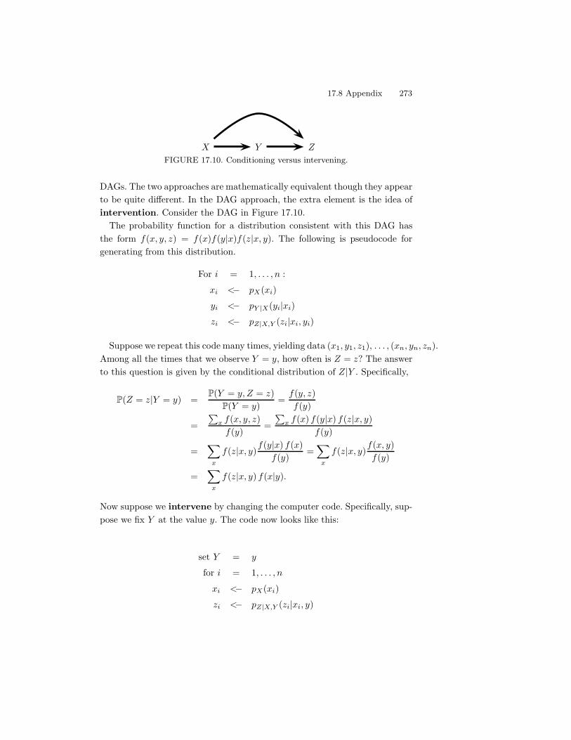
17.8 Appendix 273
X Y Z
FIGURE 17.10. Conditioning versus intervening.
DAGs. The two approaches are mathematically equivalent though they appearto be quite di!erent. In the DAG approach, the extra element is the idea ofintervention. Consider the DAG in Figure 17.10.
The probability function for a distribution consistent with this DAG hasthe form f(x, y, z) = f(x)f(y|x)f(z|x, y). The following is pseudocode forgenerating from this distribution.
For i = 1, . . . , n :
xi <" pX(xi)
yi <" pY |X(yi|xi)
zi <" pZ|X,Y (zi|xi, yi)
Suppose we repeat this code many times, yielding data (x1, y1, z1), . . . , (xn, yn, zn).Among all the times that we observe Y = y, how often is Z = z? The answerto this question is given by the conditional distribution of Z|Y . Specifically,
P(Z = z|Y = y) =P(Y = y, Z = z)
P(Y = y)=
f(y, z)f(y)
=0
x f(x, y, z)f(y)
=0
x f(x) f(y|x) f(z|x, y)f(y)
=*
x
f(z|x, y)f(y|x) f(x)
f(y)=*
x
f(z|x, y)f(x, y)f(y)
=*
x
f(z|x, y) f(x|y).
Now suppose we intervene by changing the computer code. Specifically, sup-pose we fix Y at the value y. The code now looks like this:
set Y = y
for i = 1, . . . , n
xi <" pX(xi)
zi <" pZ|X,Y (zi|xi, y)
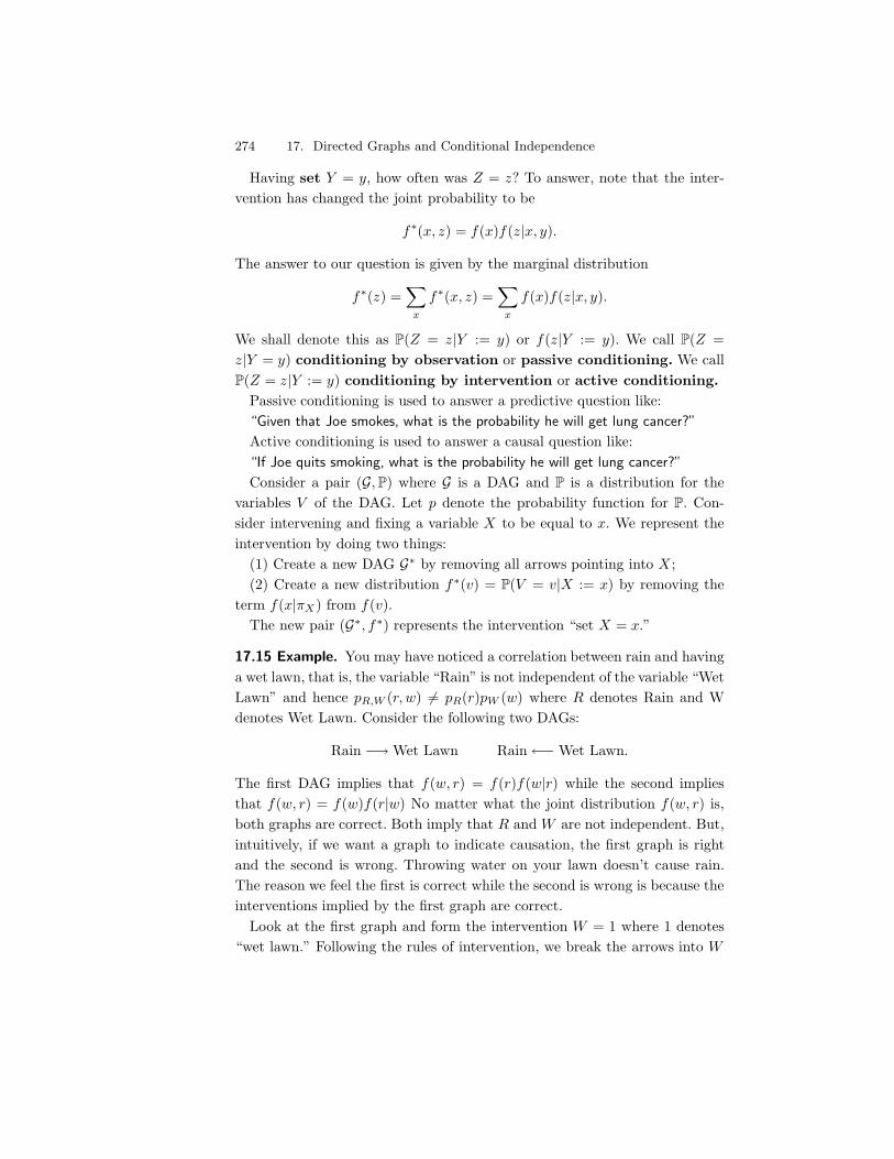
274 17. Directed Graphs and Conditional Independence
Having set Y = y, how often was Z = z? To answer, note that the inter-vention has changed the joint probability to be
f*(x, z) = f(x)f(z|x, y).
The answer to our question is given by the marginal distribution
f*(z) =*
x
f*(x, z) =*
x
f(x)f(z|x, y).
We shall denote this as P(Z = z|Y := y) or f(z|Y := y). We call P(Z =z|Y = y) conditioning by observation or passive conditioning. We callP(Z = z|Y := y) conditioning by intervention or active conditioning.
Passive conditioning is used to answer a predictive question like:“Given that Joe smokes, what is the probability he will get lung cancer?”
Active conditioning is used to answer a causal question like:“If Joe quits smoking, what is the probability he will get lung cancer?”
Consider a pair (G, P) where G is a DAG and P is a distribution for thevariables V of the DAG. Let p denote the probability function for P. Con-sider intervening and fixing a variable X to be equal to x. We represent theintervention by doing two things:
(1) Create a new DAG G* by removing all arrows pointing into X ;(2) Create a new distribution f*(v) = P(V = v|X := x) by removing the
term f(x|&X) from f(v).The new pair (G*, f*) represents the intervention “set X = x.”
17.15 Example. You may have noticed a correlation between rain and havinga wet lawn, that is, the variable “Rain” is not independent of the variable “WetLawn” and hence pR,W (r, w) (= pR(r)pW (w) where R denotes Rain and Wdenotes Wet Lawn. Consider the following two DAGs:
Rain ")Wet Lawn Rain4"Wet Lawn.
The first DAG implies that f(w, r) = f(r)f(w|r) while the second impliesthat f(w, r) = f(w)f(r|w) No matter what the joint distribution f(w, r) is,both graphs are correct. Both imply that R and W are not independent. But,intuitively, if we want a graph to indicate causation, the first graph is rightand the second is wrong. Throwing water on your lawn doesn’t cause rain.The reason we feel the first is correct while the second is wrong is because theinterventions implied by the first graph are correct.
Look at the first graph and form the intervention W = 1 where 1 denotes“wet lawn.” Following the rules of intervention, we break the arrows into W
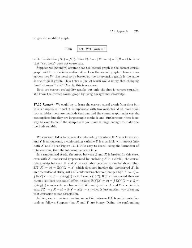
17.8 Appendix 275
to get the modified graph:
Rain set Wet Lawn =1
with distribution f*(r) = f(r). Thus P(R = r | W := w) = P(R = r) tells usthat “wet lawn” does not cause rain.
Suppose we (wrongly) assume that the second graph is the correct causalgraph and form the intervention W = 1 on the second graph. There are noarrows into W that need to be broken so the intervention graph is the sameas the original graph. Thus f*(r) = f(r|w) which would imply that changing“wet” changes “rain.” Clearly, this is nonsense.
Both are correct probability graphs but only the first is correct causally.We know the correct causal graph by using background knowledge.
17.16 Remark. We could try to learn the correct causal graph from data butthis is dangerous. In fact it is impossible with two variables. With more thantwo variables there are methods that can find the causal graph under certainassumptions but they are large sample methods and, furthermore, there is noway to ever know if the sample size you have is large enough to make themethods reliable.
We can use DAGs to represent confounding variables. If X is a treatmentand Y is an outcome, a confounding variable Z is a variable with arrows intoboth X and Y ; see Figure 17.11. It is easy to check, using the formalism ofinterventions, that the following facts are true:
In a randomized study, the arrow between Z and X is broken. In this case,even with Z unobserved (represented by enclosing Z in a circle), the causalrelationship between X and Y is estimable because it can be shown thatE(Y |X := x) = E(Y |X = x) which does not involve the unobserved Z. Inan observational study, with all confounders observed, we get E(Y |X := x) =8
E(Y |X = x, Z = z)dFZ(z) as in formula (16.7). If Z is unobserved then wecannot estimate the causal e!ect because E(Y |X := x) =
8E(Y |X = x, Z =
z)dFZ(z) involves the unobserved Z. We can’t just use X and Y since in thiscase. P(Y = y|X = x) (= P(Y = y|X := x) which is just another way of sayingthat causation is not association.
In fact, we can make a precise connection between DAGs and counterfac-tuals as follows. Suppose that X and Y are binary. Define the confounding
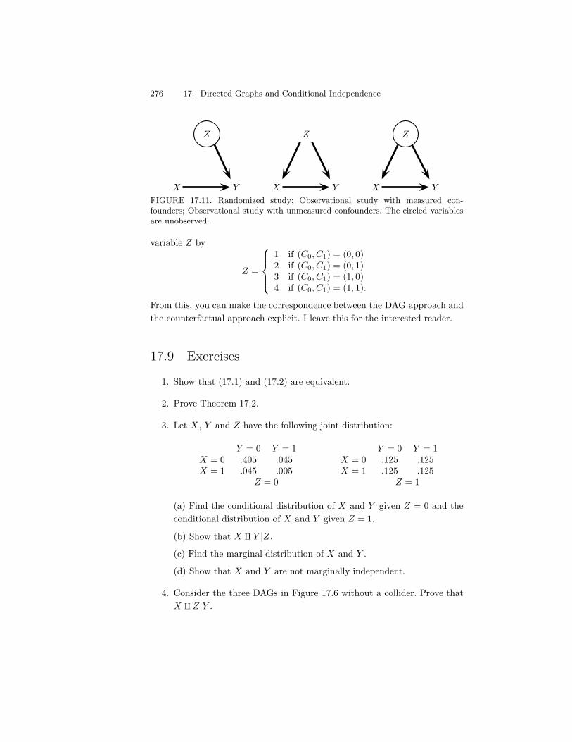
276 17. Directed Graphs and Conditional Independence
X Y
Z
X Y
Z
X Y
Z
FIGURE 17.11. Randomized study; Observational study with measured con-founders; Observational study with unmeasured confounders. The circled variablesare unobserved.
variable Z by
Z =
4556
557
1 if (C0, C1) = (0, 0)2 if (C0, C1) = (0, 1)3 if (C0, C1) = (1, 0)4 if (C0, C1) = (1, 1).
From this, you can make the correspondence between the DAG approach andthe counterfactual approach explicit. I leave this for the interested reader.
17.9 Exercises
1. Show that (17.1) and (17.2) are equivalent.
2. Prove Theorem 17.2.
3. Let X , Y and Z have the following joint distribution:
Y = 0 Y = 1 Y = 0 Y = 1X = 0 .405 .045 X = 0 .125 .125X = 1 .045 .005 X = 1 .125 .125
Z = 0 Z = 1
(a) Find the conditional distribution of X and Y given Z = 0 and theconditional distribution of X and Y given Z = 1.
(b) Show that X ! Y |Z.
(c) Find the marginal distribution of X and Y .
(d) Show that X and Y are not marginally independent.
4. Consider the three DAGs in Figure 17.6 without a collider. Prove thatX ! Z|Y .
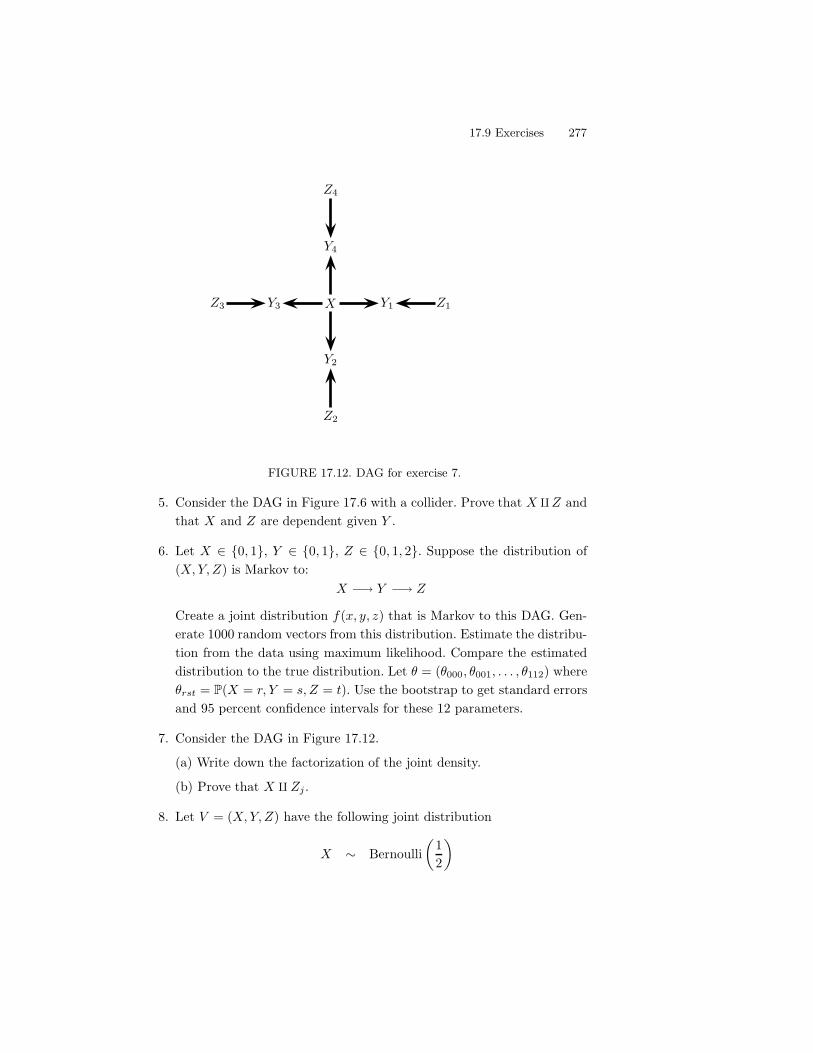
17.9 Exercises 277
X Y1 Z1Y3Z3
Y4
Z4
Y2
Z2
FIGURE 17.12. DAG for exercise 7.
5. Consider the DAG in Figure 17.6 with a collider. Prove that X !Z andthat X and Z are dependent given Y .
6. Let X $ {0, 1}, Y $ {0, 1}, Z $ {0, 1, 2}. Suppose the distribution of(X, Y, Z) is Markov to:
X ") Y ") Z
Create a joint distribution f(x, y, z) that is Markov to this DAG. Gen-erate 1000 random vectors from this distribution. Estimate the distribu-tion from the data using maximum likelihood. Compare the estimateddistribution to the true distribution. Let 0 = (0000, 0001, . . . , 0112) where0rst = P(X = r, Y = s, Z = t). Use the bootstrap to get standard errorsand 95 percent confidence intervals for these 12 parameters.
7. Consider the DAG in Figure 17.12.
(a) Write down the factorization of the joint density.
(b) Prove that X ! Zj .
8. Let V = (X, Y, Z) have the following joint distribution
X ! Bernoulli-
12
.
278 17. Directed Graphs and Conditional Independence
Y | X = x ! Bernoulli-
e4x$2
1 + e4x$2
.
Z | X = x, Y = y ! Bernoulli-
e2(x+y)$2
1 + e2(x+y)$2
..
(a) Find an expression for P(Z = z | Y = y). In particular, find P(Z =1 | Y = 1).
(b) Write a program to simulate the model. Conduct a simulation andcompute P(Z = 1 | Y = 1) empirically. Plot this as a function ofthe simulation size N . It should converge to the theoretical value youcomputed in (a).
(c) (Refers to material in the appendix.) Write down an expression forP(Z = 1 | Y := y). In particular, find P(Z = 1 | Y := 1).
(d) (Refers to material in the appendix.) Modify your program to sim-ulate the intervention “set Y = 1.” Conduct a simulation and computeP(Z = 1 | Y := 1) empirically. Plot this as a function of the simulationsize N . It should converge to the theoretical value you computed in (c).
9. This is a continuous, Gaussian version of the last question. Let V =(X, Y, Z) have the following joint distribution
X ! Normal (0, 1)
Y | X = x ! Normal ()x, 1)
Z | X = x, Y = y ! Normal ((y + /x, 1).
Here, ),( and / are fixed parameters. economists refer to models likethis as structural equation models.
(a) Find an explicit expression for f(z | y) and E(Z | Y = y) =8
zf(z |y)dz.
(b) (Refers to material in the appendix.) Find an explicit expressionfor f(z | Y := y) and then find E(Z | Y := y) 0
8zf(z | Y := y)dy.
Compare to (b).
(c) Find the joint distribution of (Y, Z). Find the correlation + betweenY and Z.
(d) (Refers to material in the appendix.) Suppose that X is not observedand we try to make causal conclusions from the marginal distribution of(Y, Z). (Think of X as unobserved confounding variables.) In particular,
17.9 Exercises 279
suppose we declare that Y causes Z if + (= 0 and we declare that Y doesnot cause Z if + = 0. Show that this will lead to erroneous conclusions.
(e) (Refers to material in the appendix.) Suppose we conduct a ran-domized experiment in which Y is randomly assigned. To be concrete,suppose that
X ! Normal(0, 1)
Y ! Normal(), 1)
Z | X = x, Y = y ! Normal((y + /x, 1).
Show that the method in (d) now yields correct conclusions (i.e., + = 0if and only if f(z | Y := y) does not depend on y).

This is page 280Printer: Opaque this

This is page 281Printer: Opaque this
18Undirected Graphs
Undirected graphs are an alternative to directed graphs for representing in-dependence relations. Since both directed and undirected graphs are used inpractice, it is a good idea to be facile with both. The main di!erence betweenthe two is that the rules for reading independence relations from the graphare di!erent.
18.1 Undirected Graphs
An undirected graph G = (V, E) has a finite set V of vertices (or nodes)and a set E of edges (or arcs) consisting of pairs of vertices. The verticescorrespond to random variables X, Y, Z, . . . and edges are written as unorderedpairs. For example, (X, Y ) $ E means that X and Y are joined by an edge.An example of a graph is in Figure 18.1.
Two vertices are adjacent, written X ! Y , if there is an edge betweenthem. In Figure 18.1, X and Y are adjacent but X and Z are not adjacent. Asequence X0, . . . , Xn is called a path if Xi$1 ! Xi for each i. In Figure 18.1,X, Y, Z is a path. A graph is complete if there is an edge between every pairof vertices. A subset U & V of vertices together with their edges is called asubgraph.
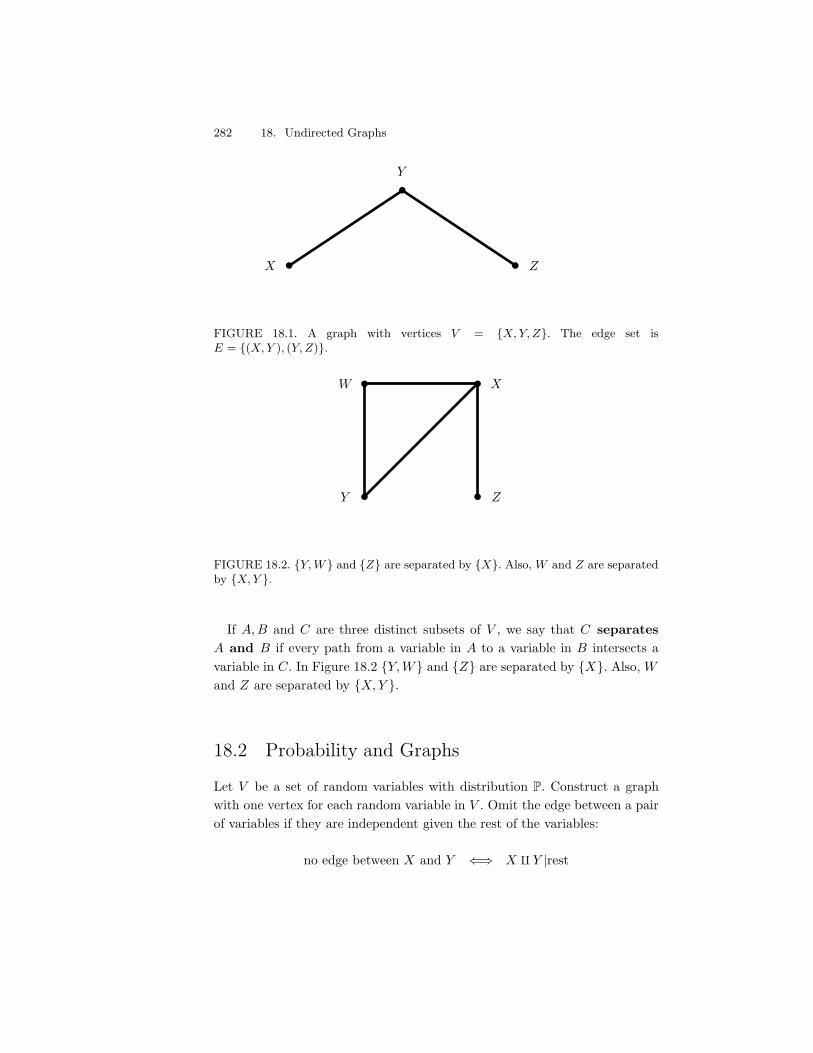
282 18. Undirected Graphs
X
Y
Z
FIGURE 18.1. A graph with vertices V = {X, Y, Z}. The edge set isE = {(X, Y ), (Y, Z)}.
Y
W X
Z
FIGURE 18.2. {Y, W} and {Z} are separated by {X}. Also, W and Z are separatedby {X, Y }.
If A, B and C are three distinct subsets of V , we say that C separatesA and B if every path from a variable in A to a variable in B intersects avariable in C. In Figure 18.2 {Y, W} and {Z} are separated by {X}. Also, W
and Z are separated by {X, Y }.
18.2 Probability and Graphs
Let V be a set of random variables with distribution P. Construct a graphwith one vertex for each random variable in V . Omit the edge between a pairof variables if they are independent given the rest of the variables:
no edge between X and Y 5+ X ! Y |rest
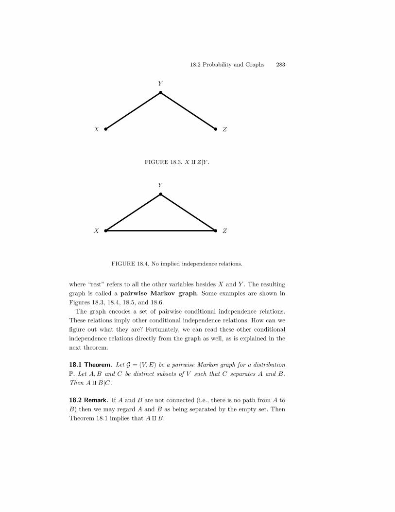
18.2 Probability and Graphs 283
X
Y
Z
FIGURE 18.3. X ! Z|Y .
X
Y
Z
FIGURE 18.4. No implied independence relations.
where “rest” refers to all the other variables besides X and Y . The resultinggraph is called a pairwise Markov graph. Some examples are shown inFigures 18.3, 18.4, 18.5, and 18.6.
The graph encodes a set of pairwise conditional independence relations.These relations imply other conditional independence relations. How can wefigure out what they are? Fortunately, we can read these other conditionalindependence relations directly from the graph as well, as is explained in thenext theorem.
18.1 Theorem. Let G = (V, E) be a pairwise Markov graph for a distributionP. Let A, B and C be distinct subsets of V such that C separates A and B.Then A ! B|C.
18.2 Remark. If A and B are not connected (i.e., there is no path from A toB) then we may regard A and B as being separated by the empty set. ThenTheorem 18.1 implies that A ! B.
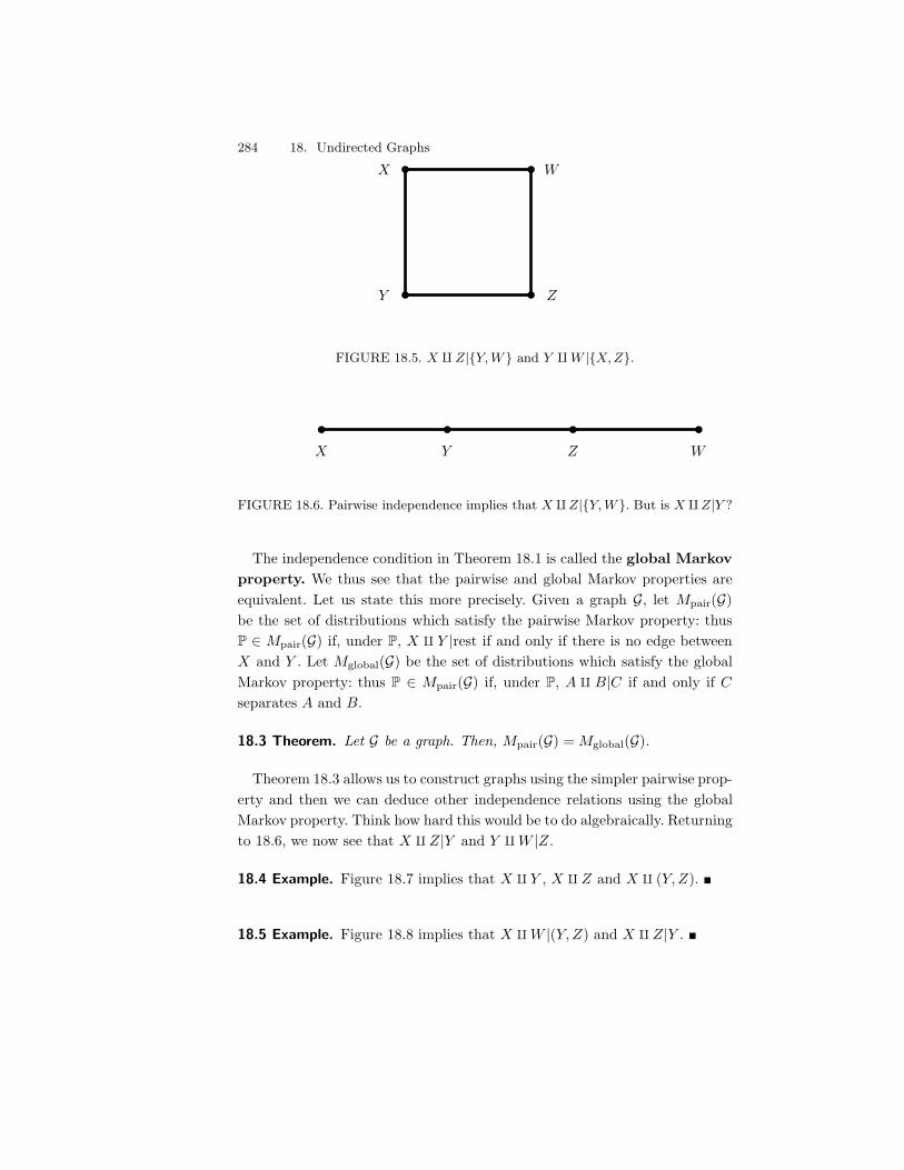
284 18. Undirected Graphs
Y
X W
Z
FIGURE 18.5. X ! Z|{Y, W} and Y ! W |{X, Z}.
X Y Z W
FIGURE 18.6. Pairwise independence implies that X !Z|{Y, W}. But is X !Z|Y ?
The independence condition in Theorem 18.1 is called the global Markovproperty. We thus see that the pairwise and global Markov properties areequivalent. Let us state this more precisely. Given a graph G, let Mpair(G)be the set of distributions which satisfy the pairwise Markov property: thusP $ Mpair(G) if, under P, X ! Y |rest if and only if there is no edge betweenX and Y . Let Mglobal(G) be the set of distributions which satisfy the globalMarkov property: thus P $ Mpair(G) if, under P, A ! B|C if and only if C
separates A and B.
18.3 Theorem. Let G be a graph. Then, Mpair(G) = Mglobal(G).
Theorem 18.3 allows us to construct graphs using the simpler pairwise prop-erty and then we can deduce other independence relations using the globalMarkov property. Think how hard this would be to do algebraically. Returningto 18.6, we now see that X ! Z|Y and Y ! W |Z.
18.4 Example. Figure 18.7 implies that X ! Y , X ! Z and X ! (Y, Z). !
18.5 Example. Figure 18.8 implies that X ! W |(Y, Z) and X ! Z|Y . !
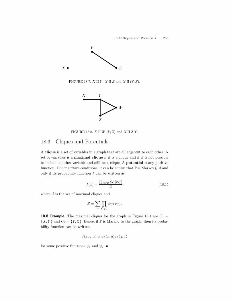
18.3 Cliques and Potentials 285
X
Y
Z
FIGURE 18.7. X ! Y , X ! Z and X ! (Y, Z).
X Y
Z
W
FIGURE 18.8. X ! W |(Y, Z) and X ! Z|Y .
18.3 Cliques and Potentials
A clique is a set of variables in a graph that are all adjacent to each other. Aset of variables is a maximal clique if it is a clique and if it is not possibleto include another variable and still be a clique. A potential is any positivefunction. Under certain conditions, it can be shown that P is Markov G if andonly if its probability function f can be written as
f(x) =D
C#C ,C(xC)Z
(18.1)
where C is the set of maximal cliques and
Z =*
x
/
C#C,C(xC).
18.6 Example. The maximal cliques for the graph in Figure 18.1 are C1 ={X, Y } and C2 = {Y, Z}. Hence, if P is Markov to the graph, then its proba-bility function can be written
f(x, y, z) 3 ,1(x, y),2(y, z)
for some positive functions ,1 and ,2. !
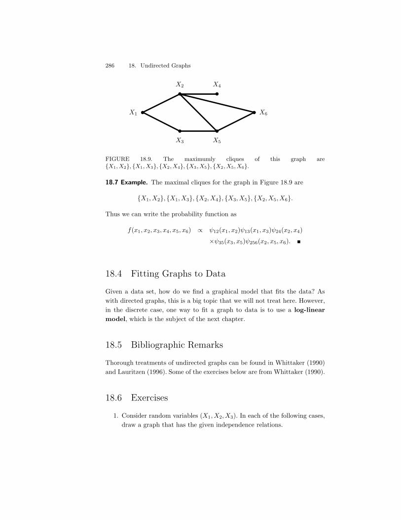
286 18. Undirected Graphs
X3 X5
X1
X2 X4
X6
FIGURE 18.9. The maximumly cliques of this graph are{X1, X2}, {X1, X3}, {X2, X4}, {X3, X5}, {X2, X5, X6}.
18.7 Example. The maximal cliques for the graph in Figure 18.9 are
{X1, X2}, {X1, X3}, {X2, X4}, {X3, X5}, {X2, X5, X6}.
Thus we can write the probability function as
f(x1, x2, x3, x4, x5, x6) 3 ,12(x1, x2),13(x1, x3),24(x2, x4)
-,35(x3, x5),256(x2, x5, x6). !
18.4 Fitting Graphs to Data
Given a data set, how do we find a graphical model that fits the data? Aswith directed graphs, this is a big topic that we will not treat here. However,in the discrete case, one way to fit a graph to data is to use a log-linearmodel, which is the subject of the next chapter.
18.5 Bibliographic Remarks
Thorough treatments of undirected graphs can be found in Whittaker (1990)and Lauritzen (1996). Some of the exercises below are from Whittaker (1990).
18.6 Exercises
1. Consider random variables (X1, X2, X3). In each of the following cases,draw a graph that has the given independence relations.
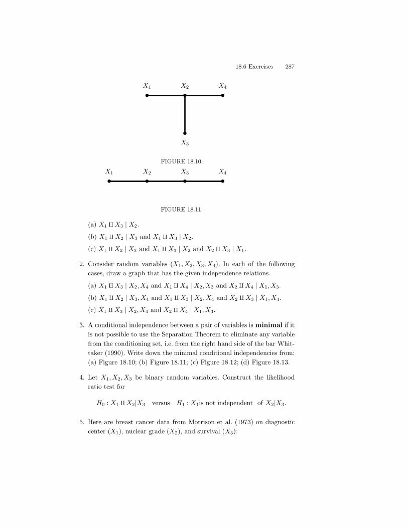
18.6 Exercises 287
X1 X2 X4
X3
FIGURE 18.10.
X1 X2 X3 X4
FIGURE 18.11.
(a) X1 ! X3 | X2.
(b) X1 ! X2 | X3 and X1 ! X3 | X2.
(c) X1 ! X2 | X3 and X1 ! X3 | X2 and X2 ! X3 | X1.
2. Consider random variables (X1, X2, X3, X4). In each of the followingcases, draw a graph that has the given independence relations.
(a) X1 ! X3 | X2, X4 and X1 ! X4 | X2, X3 and X2 ! X4 | X1, X3.
(b) X1 ! X2 | X3, X4 and X1 ! X3 | X2, X4 and X2 ! X3 | X1, X4.
(c) X1 ! X3 | X2, X4 and X2 ! X4 | X1, X3.
3. A conditional independence between a pair of variables is minimal if itis not possible to use the Separation Theorem to eliminate any variablefrom the conditioning set, i.e. from the right hand side of the bar Whit-taker (1990). Write down the minimal conditional independencies from:(a) Figure 18.10; (b) Figure 18.11; (c) Figure 18.12; (d) Figure 18.13.
4. Let X1, X2, X3 be binary random variables. Construct the likelihoodratio test for
H0 : X1 ! X2|X3 versus H1 : X1is not independent of X2|X3.
5. Here are breast cancer data from Morrison et al. (1973) on diagnosticcenter (X1), nuclear grade (X2), and survival (X3):
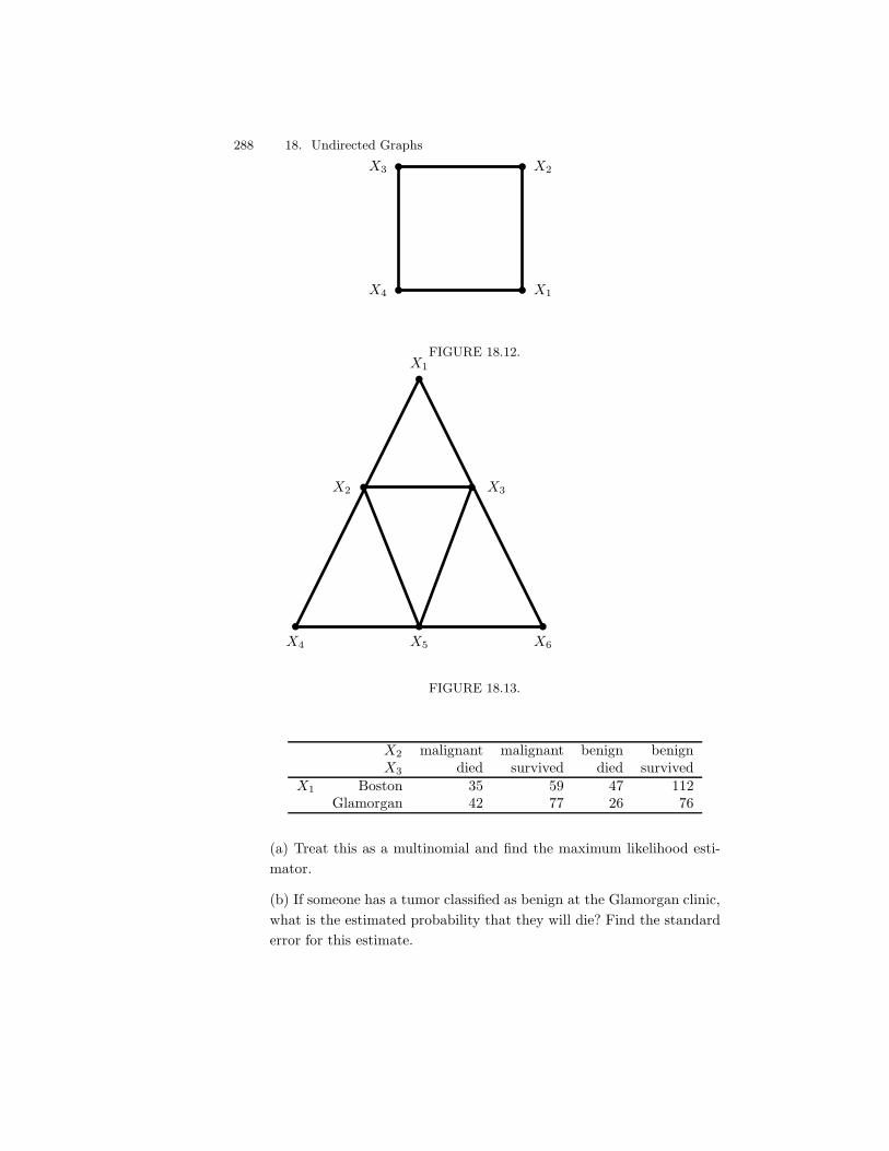
288 18. Undirected Graphs
X4
X3 X2
X1
FIGURE 18.12.
X4
X2 X3
X1
X6X5
FIGURE 18.13.
X2 malignant malignant benign benignX3 died survived died survived
X1 Boston 35 59 47 112Glamorgan 42 77 26 76
(a) Treat this as a multinomial and find the maximum likelihood esti-mator.
(b) If someone has a tumor classified as benign at the Glamorgan clinic,what is the estimated probability that they will die? Find the standarderror for this estimate.

18.6 Exercises 289
(c) Test the following hypotheses:
X1 ! X2|X3 versus X1 !""""# X2|X3
X1 ! X3|X2 versus X1 !""""# X3|X2
X2 ! X3|X1 versus X2 !""""# X3|X1
Use the test from question 4. Based on the results of your tests, drawand interpret the resulting graph.

This is page 290Printer: Opaque this
This is page 291Printer: Opaque this
19Log-Linear Models
In this chapter we study log-linear models which are useful for modelingmultivariate discrete data. There is a strong connection between log-linearmodels and undirected graphs.
19.1 The Log-Linear Model
Let X = (X1, . . . , Xm) be a discrete random vector with probability function
f(x) = P(X = x) = P(X1 = x1, . . . , Xm = xm)
where x = (x1, . . . , xm). Let rj be the number of values that Xj takes. Withoutloss of generality, we can assume that Xj $ {0, 1, . . . , rj " 1}. Suppose nowthat we have n such random vectors. We can think of the data as a samplefrom a Multinomial with N = r1 - r2 - · · ·- rm categories. The data can berepresented as counts in a r1-r2- · · ·-rm table. Let p = (p1, . . . , pN ) denotethe multinomial parameter.
Let S = {1, . . . , m}. Given a vector x = (x1, . . . , xm) and a subset A & S,let xA = (xj : j $ A). For example, if A = {1, 3} then xA = (x1, x3).
292 19. Log-Linear Models
19.1 Theorem. The joint probability function f(x) of a single random vectorX = (X1, . . . , Xm) can be written as
log f(x) =*
A,S
,A(x) (19.1)
where the sum is over all subsets A of S = {1, . . . , m} and the ,’s satisfy thefollowing conditions:
1. ,-(x) is a constant;
2. For every A & S, ,A(x) is only a function of xA and not the rest of thex&
js.
3. If i $ A and xi = 0, then ,A(x) = 0.
The formula in equation (19.1) is called the log-linear expansion of f .Each ,A(x) may depend on some unknown parameters (A. Let ( = ((A :A & S) be the set of all these parameters. We will write f(x) = f(x;() whenwe want to emphasize the dependence on the unknown parameters (.
In terms of the multinomial, the parameter space is
P ='
p = (p1, . . . , pN ) : pj * 0,N*
j=1
pj = 12
.
This is an N " 1 dimensional space. In the log-linear representation, the pa-rameter space is
" ='( = ((1, . . . ,(N ) : ( = ((p), p $ P
2
where ((p) is the set of ( values associated with p. The set " is a N " 1dimensional surface in RN . We can always go back and forth between the twoparameterizations we can write ( = ((p) and p = p(().
19.2 Example. Let X ! Bernoulli(p) where 0 < p < 1. We can write theprobability mass function for X as
f(x) = px(1" p)1$x = px1 p1$x
2
for x = 0, 1, where p1 = p and p2 = 1" p. Hence,
log f(x) = ,-(x) + ,1(x)
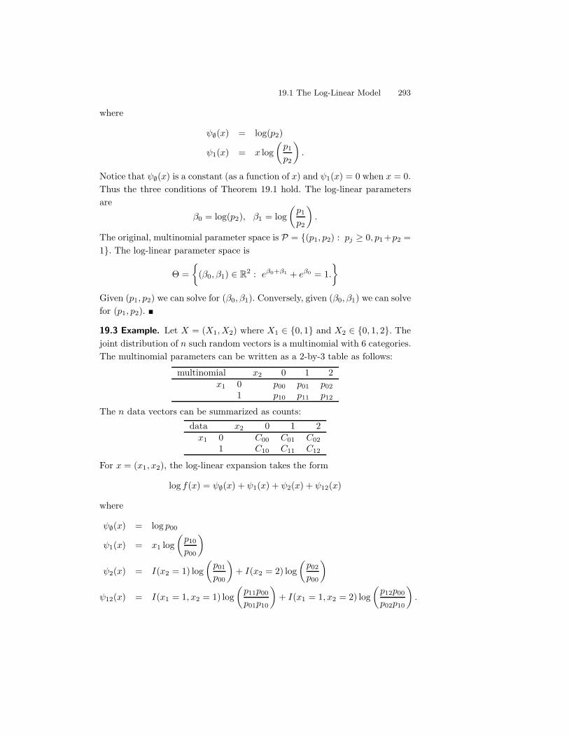
19.1 The Log-Linear Model 293
where
,-(x) = log(p2)
,1(x) = x log-
p1
p2
..
Notice that ,-(x) is a constant (as a function of x) and ,1(x) = 0 when x = 0.Thus the three conditions of Theorem 19.1 hold. The log-linear parametersare
(0 = log(p2), (1 = log-
p1
p2
..
The original, multinomial parameter space is P = {(p1, p2) : pj * 0, p1+p2 =1}. The log-linear parameter space is
" ='
((0,(1) $ R2 : e"0+"1 + e"0 = 1.
2
Given (p1, p2) we can solve for ((0,(1). Conversely, given ((0,(1) we can solvefor (p1, p2). !
19.3 Example. Let X = (X1, X2) where X1 $ {0, 1} and X2 $ {0, 1, 2}. Thejoint distribution of n such random vectors is a multinomial with 6 categories.The multinomial parameters can be written as a 2-by-3 table as follows:
multinomial x2 0 1 2x1 0 p00 p01 p02
1 p10 p11 p12
The n data vectors can be summarized as counts:data x2 0 1 2
x1 0 C00 C01 C02
1 C10 C11 C12
For x = (x1, x2), the log-linear expansion takes the form
log f(x) = ,-(x) + ,1(x) + ,2(x) + ,12(x)
where
,-(x) = log p00
,1(x) = x1 log-
p10
p00
.
,2(x) = I(x2 = 1) log-
p01
p00
.+ I(x2 = 2) log
-p02
p00
.
,12(x) = I(x1 = 1, x2 = 1) log-
p11p00
p01p10
.+ I(x1 = 1, x2 = 2) log
-p12p00
p02p10
..
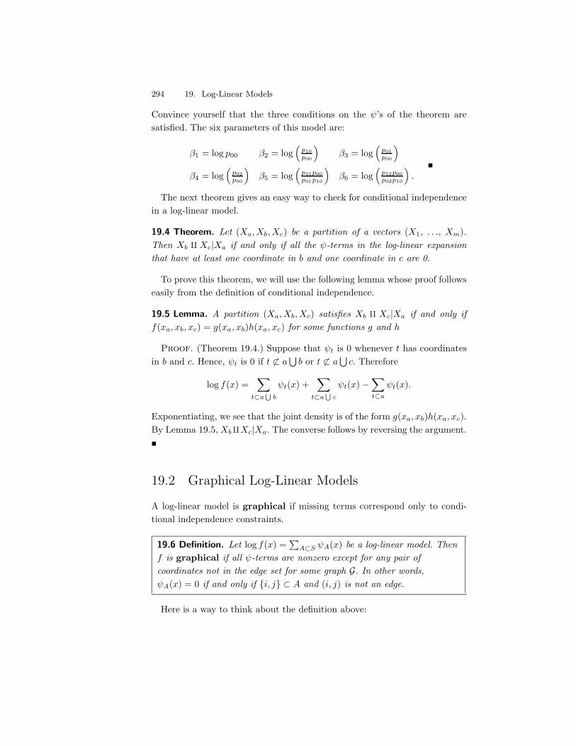
294 19. Log-Linear Models
Convince yourself that the three conditions on the ,’s of the theorem aresatisfied. The six parameters of this model are:
(1 = log p00 (2 = log+
p10p00
,(3 = log
+p01p00
,
(4 = log+
p02p00
,(5 = log
+p11p00p01p10
,(6 = log
+p12p00p02p10
,.
!
The next theorem gives an easy way to check for conditional independencein a log-linear model.
19.4 Theorem. Let (Xa, Xb, Xc) be a partition of a vectors (X1, . . ., Xm).Then Xb ! Xc|Xa if and only if all the ,-terms in the log-linear expansionthat have at least one coordinate in b and one coordinate in c are 0.
To prove this theorem, we will use the following lemma whose proof followseasily from the definition of conditional independence.
19.5 Lemma. A partition (Xa, Xb, Xc) satisfies Xb ! Xc|Xa if and only iff(xa, xb, xc) = g(xa, xb)h(xa, xc) for some functions g and h
Proof. (Theorem 19.4.) Suppose that ,t is 0 whenever t has coordinatesin b and c. Hence, ,t is 0 if t (& a
&b or t (& a
&c. Therefore
log f(x) =*
t,a&
b
,t(x) +*
t,a&
c
,t(x)"*
t,a
,t(x).
Exponentiating, we see that the joint density is of the form g(xa, xb)h(xa, xc).By Lemma 19.5, Xb!Xc|Xa. The converse follows by reversing the argument.!
19.2 Graphical Log-Linear Models
A log-linear model is graphical if missing terms correspond only to condi-tional independence constraints.
19.6 Definition. Let log f(x) =0
A,S ,A(x) be a log-linear model. Thenf is graphical if all ,-terms are nonzero except for any pair ofcoordinates not in the edge set for some graph G. In other words,,A(x) = 0 if and only if {i, j} & A and (i, j) is not an edge.
Here is a way to think about the definition above:
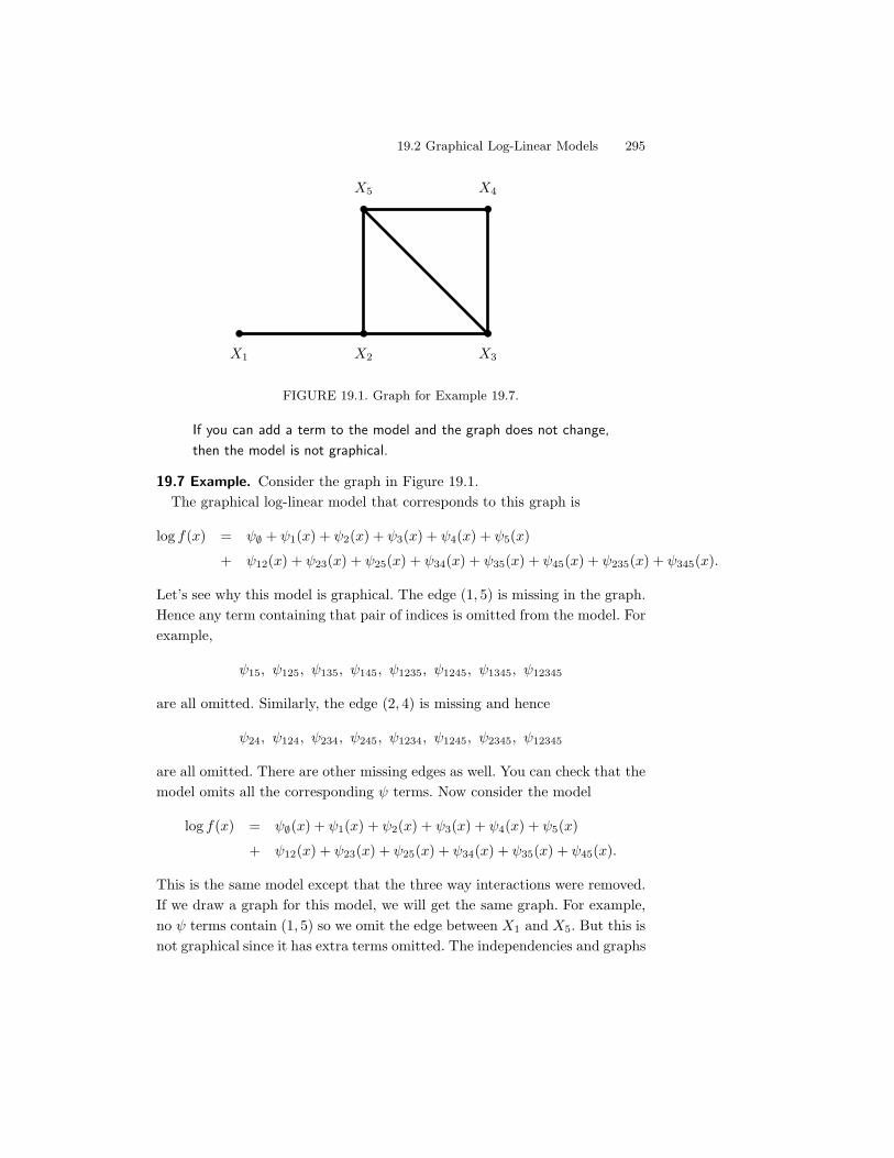
19.2 Graphical Log-Linear Models 295
X1 X2 X3
X5 X4
FIGURE 19.1. Graph for Example 19.7.
If you can add a term to the model and the graph does not change,
then the model is not graphical.
19.7 Example. Consider the graph in Figure 19.1.The graphical log-linear model that corresponds to this graph is
log f(x) = ,- + ,1(x) + ,2(x) + ,3(x) + ,4(x) + ,5(x)
+ ,12(x) + ,23(x) + ,25(x) + ,34(x) + ,35(x) + ,45(x) + ,235(x) + ,345(x).
Let’s see why this model is graphical. The edge (1, 5) is missing in the graph.Hence any term containing that pair of indices is omitted from the model. Forexample,
,15, ,125, ,135, ,145, ,1235, ,1245, ,1345, ,12345
are all omitted. Similarly, the edge (2, 4) is missing and hence
,24, ,124, ,234, ,245, ,1234, ,1245, ,2345, ,12345
are all omitted. There are other missing edges as well. You can check that themodel omits all the corresponding , terms. Now consider the model
log f(x) = ,-(x) + ,1(x) + ,2(x) + ,3(x) + ,4(x) + ,5(x)
+ ,12(x) + ,23(x) + ,25(x) + ,34(x) + ,35(x) + ,45(x).
This is the same model except that the three way interactions were removed.If we draw a graph for this model, we will get the same graph. For example,no , terms contain (1, 5) so we omit the edge between X1 and X5. But this isnot graphical since it has extra terms omitted. The independencies and graphs
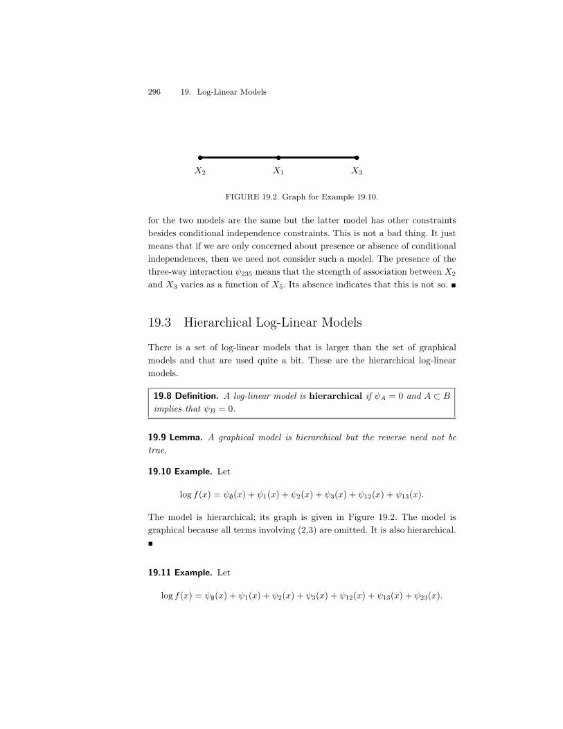
296 19. Log-Linear Models
X2 X1 X3
FIGURE 19.2. Graph for Example 19.10.
for the two models are the same but the latter model has other constraintsbesides conditional independence constraints. This is not a bad thing. It justmeans that if we are only concerned about presence or absence of conditionalindependences, then we need not consider such a model. The presence of thethree-way interaction ,235 means that the strength of association between X2
and X3 varies as a function of X5. Its absence indicates that this is not so. !
19.3 Hierarchical Log-Linear Models
There is a set of log-linear models that is larger than the set of graphicalmodels and that are used quite a bit. These are the hierarchical log-linearmodels.
19.8 Definition. A log-linear model is hierarchical if ,A = 0 and A & B
implies that ,B = 0.
19.9 Lemma. A graphical model is hierarchical but the reverse need not betrue.
19.10 Example. Let
log f(x) = ,-(x) + ,1(x) + ,2(x) + ,3(x) + ,12(x) + ,13(x).
The model is hierarchical; its graph is given in Figure 19.2. The model isgraphical because all terms involving (2,3) are omitted. It is also hierarchical.!
19.11 Example. Let
log f(x) = ,-(x) + ,1(x) + ,2(x) + ,3(x) + ,12(x) + ,13(x) + ,23(x).
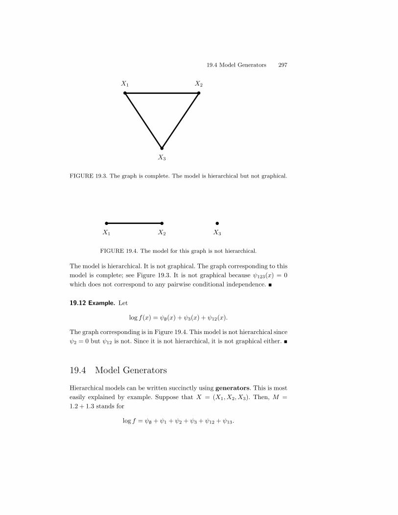
19.4 Model Generators 297
X3
X1 X2
FIGURE 19.3. The graph is complete. The model is hierarchical but not graphical.
X1 X2 X3
FIGURE 19.4. The model for this graph is not hierarchical.
The model is hierarchical. It is not graphical. The graph corresponding to thismodel is complete; see Figure 19.3. It is not graphical because ,123(x) = 0which does not correspond to any pairwise conditional independence. !
19.12 Example. Let
log f(x) = ,-(x) + ,3(x) + ,12(x).
The graph corresponding is in Figure 19.4. This model is not hierarchical since,2 = 0 but ,12 is not. Since it is not hierarchical, it is not graphical either. !
19.4 Model Generators
Hierarchical models can be written succinctly using generators. This is mosteasily explained by example. Suppose that X = (X1, X2, X3). Then, M =1.2 + 1.3 stands for
log f = ,- + ,1 + ,2 + ,3 + ,12 + ,13.
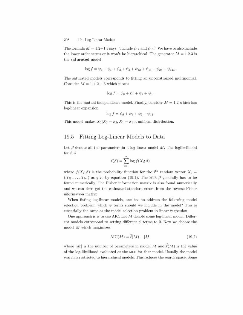
298 19. Log-Linear Models
The formula M = 1.2+1.3 says: “include ,12 and ,13.” We have to also includethe lower order terms or it won’t be hierarchical. The generator M = 1.2.3 isthe saturated model
log f = ,- + ,1 + ,2 + ,3 + ,12 + ,13 + ,23 + ,123.
The saturated models corresponds to fitting an unconstrained multinomial.Consider M = 1 + 2 + 3 which means
log f = ,- + ,1 + ,2 + ,3.
This is the mutual independence model. Finally, consider M = 1.2 which haslog-linear expansion
log f = ,- + ,1 + ,2 + ,12.
This model makes X3|X2 = x2, X1 = x1 a uniform distribution.
19.5 Fitting Log-Linear Models to Data
Let ( denote all the parameters in a log-linear model M . The loglikelihoodfor ( is
4(() =n*
i=1
log f(Xi;()
where f(Xi;() is the probability function for the ith random vector Xi =(Xi1, . . . , Xim) as give by equation (19.1). The mle 1( generally has to befound numerically. The Fisher information matrix is also found numericallyand we can then get the estimated standard errors from the inverse Fisherinformation matrix.
When fitting log-linear models, one has to address the following modelselection problem: which , terms should we include in the model? This isessentially the same as the model selection problem in linear regression.
One approach is is to use AIC. Let M denote some log-linear model. Di!er-ent models correspond to setting di!erent , terms to 0. Now we choose themodel M which maximizes
AIC(M) = 14(M)" |M | (19.2)
where |M | is the number of parameters in model M and 14(M) is the valueof the log-likelihood evaluated at the mle for that model. Usually the modelsearch is restricted to hierarchical models. This reduces the search space. Some
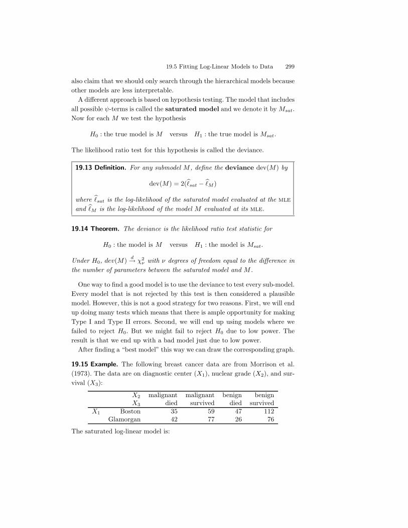
19.5 Fitting Log-Linear Models to Data 299
also claim that we should only search through the hierarchical models becauseother models are less interpretable.
A di!erent approach is based on hypothesis testing. The model that includesall possible ,-terms is called the saturated model and we denote it by Msat.Now for each M we test the hypothesis
H0 : the true model is M versus H1 : the true model is Msat.
The likelihood ratio test for this hypothesis is called the deviance.
19.13 Definition. For any submodel M , define the deviance dev(M) by
dev(M) = 2(14sat " 14M )
where 14sat is the log-likelihood of the saturated model evaluated at the mle
and 14M is the log-likelihood of the model M evaluated at its mle.
19.14 Theorem. The deviance is the likelihood ratio test statistic for
H0 : the model is M versus H1 : the model is Msat.
Under H0, dev(M) d) !2$ with * degrees of freedom equal to the di!erence in
the number of parameters between the saturated model and M .
One way to find a good model is to use the deviance to test every sub-model.Every model that is not rejected by this test is then considered a plausiblemodel. However, this is not a good strategy for two reasons. First, we will endup doing many tests which means that there is ample opportunity for makingType I and Type II errors. Second, we will end up using models where wefailed to reject H0. But we might fail to reject H0 due to low power. Theresult is that we end up with a bad model just due to low power.
After finding a “best model” this way we can draw the corresponding graph.
19.15 Example. The following breast cancer data are from Morrison et al.(1973). The data are on diagnostic center (X1), nuclear grade (X2), and sur-vival (X3):
X2 malignant malignant benign benignX3 died survived died survived
X1 Boston 35 59 47 112Glamorgan 42 77 26 76
The saturated log-linear model is:
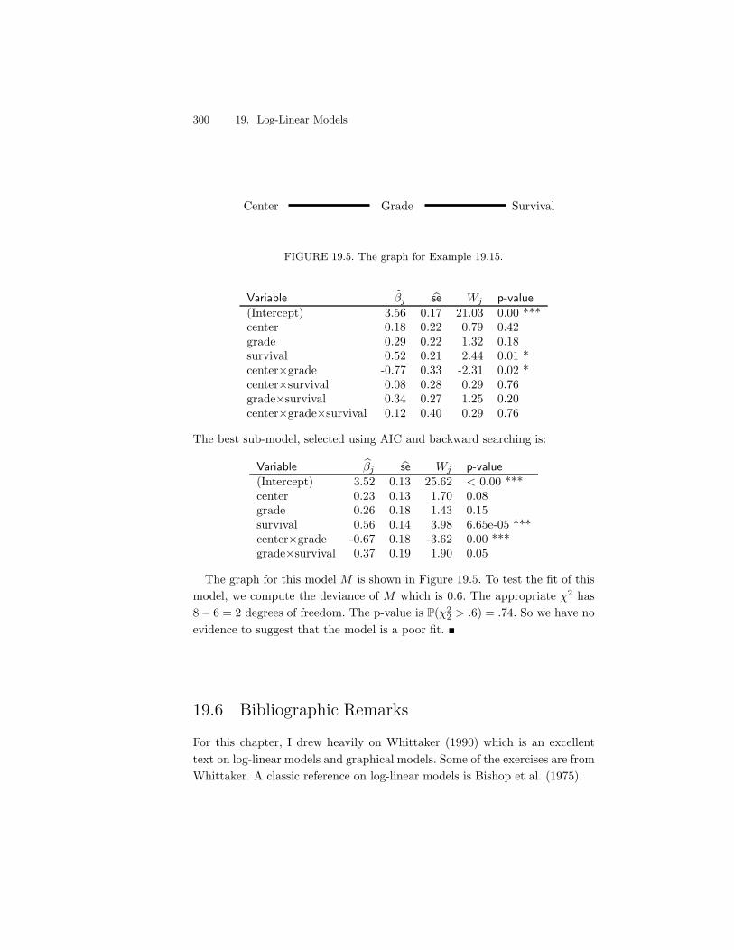
300 19. Log-Linear Models
Center Grade Survival
FIGURE 19.5. The graph for Example 19.15.
Variable 1(j 1se Wj p-value(Intercept) 3.56 0.17 21.03 0.00 ***center 0.18 0.22 0.79 0.42grade 0.29 0.22 1.32 0.18survival 0.52 0.21 2.44 0.01 *center-grade -0.77 0.33 -2.31 0.02 *center-survival 0.08 0.28 0.29 0.76grade-survival 0.34 0.27 1.25 0.20center-grade-survival 0.12 0.40 0.29 0.76
The best sub-model, selected using AIC and backward searching is:
Variable 1(j 1se Wj p-value(Intercept) 3.52 0.13 25.62 < 0.00 ***center 0.23 0.13 1.70 0.08grade 0.26 0.18 1.43 0.15survival 0.56 0.14 3.98 6.65e-05 ***center-grade -0.67 0.18 -3.62 0.00 ***grade-survival 0.37 0.19 1.90 0.05
The graph for this model M is shown in Figure 19.5. To test the fit of thismodel, we compute the deviance of M which is 0.6. The appropriate !2 has8" 6 = 2 degrees of freedom. The p-value is P(!2
2 > .6) = .74. So we have noevidence to suggest that the model is a poor fit. !
19.6 Bibliographic Remarks
For this chapter, I drew heavily on Whittaker (1990) which is an excellenttext on log-linear models and graphical models. Some of the exercises are fromWhittaker. A classic reference on log-linear models is Bishop et al. (1975).
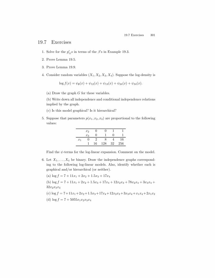
19.7 Exercises 301
19.7 Exercises
1. Solve for the p&ijs in terms of the (’s in Example 19.3.
2. Prove Lemma 19.5.
3. Prove Lemma 19.9.
4. Consider random variables (X1, X2, X3, X4). Suppose the log-density is
log f(x) = ,-(x) + ,12(x) + ,13(x) + ,24(x) + ,34(x).
(a) Draw the graph G for these variables.
(b) Write down all independence and conditional independence relationsimplied by the graph.
(c) Is this model graphical? Is it hierarchical?
5. Suppose that parameters p(x1, x2, x3) are proportional to the followingvalues:
x2 0 0 1 1x3 0 1 0 1
x1 0 2 8 4 161 16 128 32 256
Find the ,-terms for the log-linear expansion. Comment on the model.
6. Let X1, . . . , X4 be binary. Draw the independence graphs correspond-ing to the following log-linear models. Also, identify whether each isgraphical and/or hierarchical (or neither).
(a) log f = 7 + 11x1 + 2x2 + 1.5x3 + 17x4
(b) log f = 7 + 11x1 + 2x2 + 1.5x3 + 17x4 + 12x2x3 + 78x2x4 + 3x3x4 +32x2x3x4
(c) log f = 7+11x1+2x2+1.5x3+17x4+12x2x3+3x3x4+x1x4+2x1x2
(d) log f = 7 + 5055x1x2x3x4

This is page 302Printer: Opaque this
This is page 303Printer: Opaque this
20Nonparametric Curve Estimation
In this Chapter we discuss nonparametric estimation of probability densityfunctions and regression functions which we refer to as curve estimation orsmoothing.
In Chapter 7 we saw that it is possible to consistently estimate a cumulativedistribution function F without making any assumptions about F . If we wantto estimate a probability density function f(x) or a regression function r(x) =E(Y |X = x) the situation is di!erent. We cannot estimate these functionsconsistently without making some smoothness assumptions. Correspondingly,we need to perform some sort of smoothing operation on the data.
An example of a density estimator is a histogram, which we discuss indetail in Section 20.2. To form a histogram estimator of a density f , we dividethe real line to disjoint sets called bins. The histogram estimator is a piecewiseconstant function where the height of the function is proportional to numberof observations in each bin; see Figure 20.3. The number of bins is an exampleof a smoothing parameter. If we smooth too much (large bins) we get ahighly biased estimator while if we smooth too little (small bins) we get ahighly variable estimator. Much of curve estimation is concerned with tryingto optimally balance variance and bias.
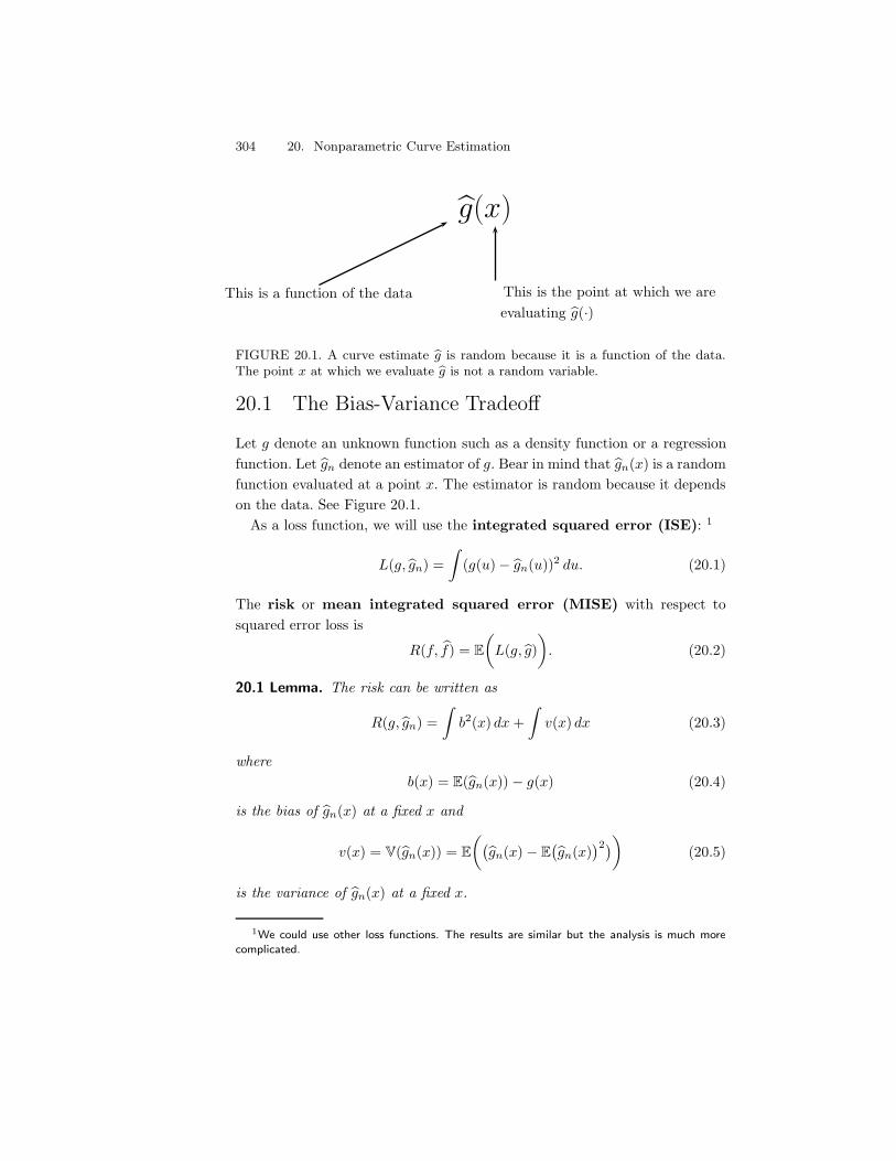
304 20. Nonparametric Curve Estimation
1g(x)
This is a function of the data This is the point at which we areevaluating 1g(·)
FIGURE 20.1. A curve estimate 1g is random because it is a function of the data.The point x at which we evaluate 1g is not a random variable.
20.1 The Bias-Variance Tradeo!
Let g denote an unknown function such as a density function or a regressionfunction. Let 1gn denote an estimator of g. Bear in mind that 1gn(x) is a randomfunction evaluated at a point x. The estimator is random because it dependson the data. See Figure 20.1.
As a loss function, we will use the integrated squared error (ISE): 1
L(g, 1gn) =9
(g(u)" 1gn(u))2 du. (20.1)
The risk or mean integrated squared error (MISE) with respect tosquared error loss is
R(f, 1f) = E-
L(g, 1g).
. (20.2)
20.1 Lemma. The risk can be written as
R(g, 1gn) =9
b2(x) dx +9
v(x) dx (20.3)
whereb(x) = E(1gn(x)) " g(x) (20.4)
is the bias of 1gn(x) at a fixed x and
v(x) = V(1gn(x)) = E-;1gn(x) " E
;1gn(x)
<2<.
(20.5)
is the variance of 1gn(x) at a fixed x.
1We could use other loss functions. The results are similar but the analysis is much morecomplicated.
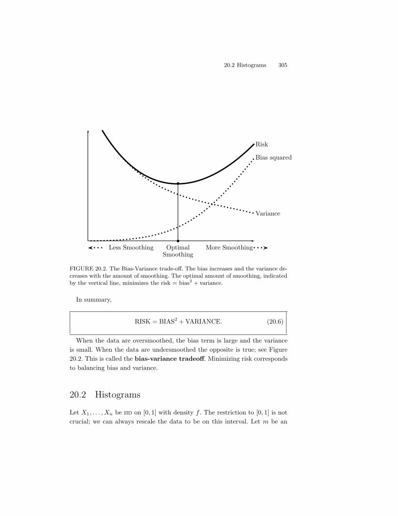
20.2 Histograms 305
Risk
Bias squared
Variance
OptimalSmoothing
More SmoothingLess Smoothing
FIGURE 20.2. The Bias-Variance trade-o". The bias increases and the variance de-creases with the amount of smoothing. The optimal amount of smoothing, indicatedby the vertical line, minimizes the risk = bias2 + variance.
In summary,
RISK = BIAS2 + VARIANCE. (20.6)
When the data are oversmoothed, the bias term is large and the varianceis small. When the data are undersmoothed the opposite is true; see Figure20.2. This is called the bias-variance tradeo". Minimizing risk correspondsto balancing bias and variance.
20.2 Histograms
Let X1, . . . , Xn be iid on [0, 1] with density f . The restriction to [0, 1] is notcrucial; we can always rescale the data to be on this interval. Let m be an
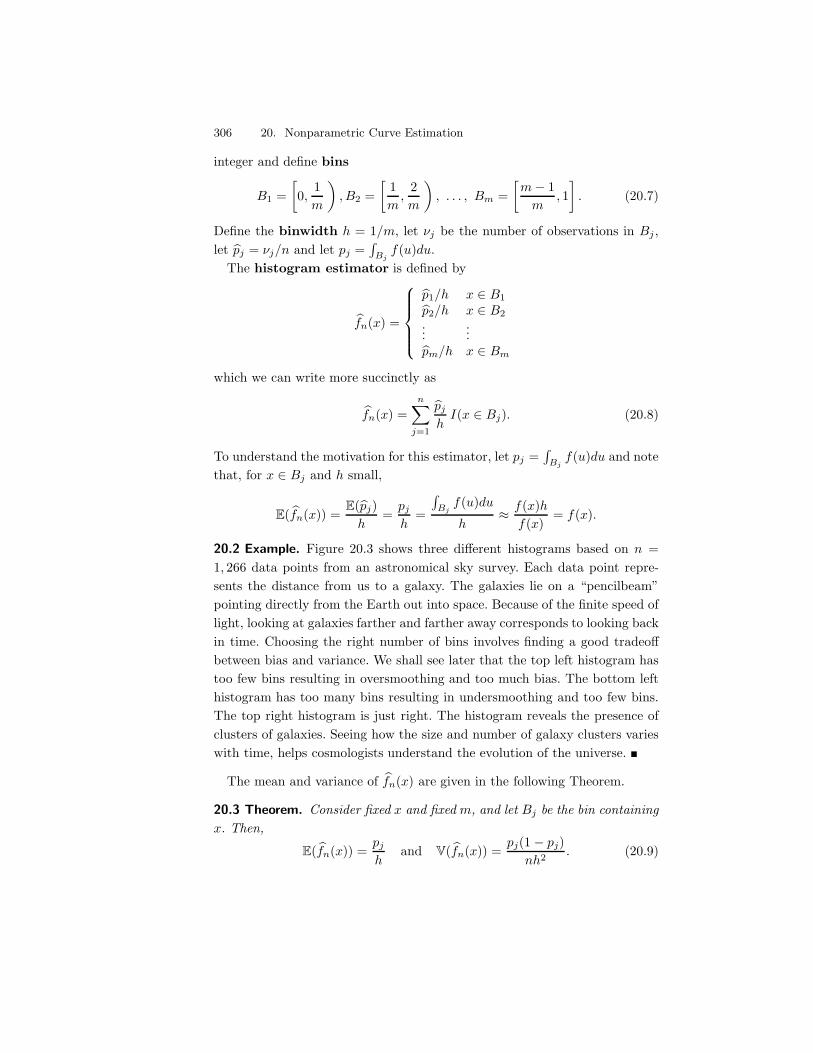
306 20. Nonparametric Curve Estimation
integer and define bins
B1 =A0,
1m
., B2 =
A1m
,2m
., . . . , Bm =
Am" 1
m, 1B
. (20.7)
Define the binwidth h = 1/m, let *j be the number of observations in Bj ,let 1pj = *j/n and let pj =
8Bj
f(u)du.The histogram estimator is defined by
1fn(x) =
45556
5557
1p1/h x $ B1
1p2/h x $ B2...
...1pm/h x $ Bm
which we can write more succinctly as
1fn(x) =n*
j=1
1pj
hI(x $ Bj). (20.8)
To understand the motivation for this estimator, let pj =8
Bjf(u)du and note
that, for x $ Bj and h small,
E( 1fn(x)) =E(1pj)
h=
pj
h=
8Bj
f(u)du
h. f(x)h
f(x)= f(x).
20.2 Example. Figure 20.3 shows three di!erent histograms based on n =1, 266 data points from an astronomical sky survey. Each data point repre-sents the distance from us to a galaxy. The galaxies lie on a “pencilbeam”pointing directly from the Earth out into space. Because of the finite speed oflight, looking at galaxies farther and farther away corresponds to looking backin time. Choosing the right number of bins involves finding a good tradeo!between bias and variance. We shall see later that the top left histogram hastoo few bins resulting in oversmoothing and too much bias. The bottom lefthistogram has too many bins resulting in undersmoothing and too few bins.The top right histogram is just right. The histogram reveals the presence ofclusters of galaxies. Seeing how the size and number of galaxy clusters varieswith time, helps cosmologists understand the evolution of the universe. !
The mean and variance of 1fn(x) are given in the following Theorem.
20.3 Theorem. Consider fixed x and fixed m, and let Bj be the bin containingx. Then,
E( 1fn(x)) =pj
hand V( 1fn(x)) =
pj(1 " pj)nh2
. (20.9)
20.2 Histograms 307
Oversmoothed
0.00 0.05 0.10 0.15 0.20
02
46
810
1214
Just Right
0.00 0.05 0.10 0.15 0.20
010
2030
4050
60
Undersmoothed
0.00 0.05 0.10 0.15 0.20
020
4060
0 200 400 600 800 1000
!14
!12
!10
!8!6
number of bins
cross
valid
ation
score
FIGURE 20.3. Three versions of a histogram for the astronomy data. The top lefthistogram has too few bins. The bottom left histogram has too many bins. The topright histogram is just right. The lower, right plot shows the estimated risk versusthe number of bins.
308 20. Nonparametric Curve Estimation
Let’s take a closer look at the bias-variance tradeo! using equation (20.9).Consider some x $ Bj . For any other u $ Bj ,
f(u) . f(x) + (u " x)f &(x)
and so
pj =9
Bj
f(u)du .9
Bj
-f(x) + (u " x)f &(x)
.du
= f(x)h + hf &(x)-
h
-j " 1
2
." x
..
Therefore, the bias b(x) is
b(x) = E( 1fn(x)) " f(x) =pj
h" f(x)
.f(x)h + hf &(x)
;h;j " 1
2
<" x<
h" f(x)
= f &(x)-
h
-j " 1
2
." x
..
If cxj is the center of the bin, then9
Bj
b2(x) dx .9
Bj
(f &(x))2-
h
-j " 1
2
." x
.2
dx
. (f &(cxj))29
Bj
-h
-j " 1
2
." x
.2
dx
= (f &(cxj))2h3
12.
Therefore,9 1
0b2(x)dx =
m*
j=1
9
Bj
b2(x)dx .m*
j=1
(f &(cxj))2h3
12
=h2
12
m*
j=1
h (f &(cxj))2 .h2
12
9 1
0(f &(x))2dx.
Note that this increases as a function of h. Now consider the variance. For h
small, 1" pj . 1, so
v(x) . pj
nh2
=f(x)h + hf &(x)
;h;j " 1
2
<" x<
nh2
. f(x)nh
20.2 Histograms 309
where we have kept only the dominant term. So,9 1
0v(x)dx . 1
nh.
Note that this decreases with h. Putting all this together, we get:
20.4 Theorem. Suppose that8
(f &(u))2du <#. Then
R( 1fn, f) . h2
12
9(f &(u))2du +
1nh
. (20.10)
The value h* that minimizes (20.10) is
h* =1
n1/3
-68
(f &(u))2du
.1/3
. (20.11)
With this choice of binwidth,
R( 1fn, f) . C
n2/3(20.12)
where C = (3/4)2/3
-8(f &(u))2du
.1/3
.
Theorem 20.4 is quite revealing. We see that with an optimally chosen bin-width, the MISE decreases to 0 at rate n$2/3. By comparison, most parametricestimators converge at rate n$1. The slower rate of convergence is the pricewe pay for being nonparametric. The formula for the optimal binwidth h* isof theoretical interest but it is not useful in practice since it depends on theunknown function f .
A practical way to choose the binwidth is to estimate the risk functionand minimize over h. Recall that the loss function, which we now write as afunction of h, is
L(h) =9
( 1fn(x) " f(x))2 dx
=91f 2n (x) dx " 2
91fn(x)f(x)dx +
9f2(x) dx.
The last term does not depend on the binwidth h so minimizing the risk isequivalent to minimizing the expected value of
J(h) =91f 2n (x) dx " 2
91fn(x)f(x)dx.
310 20. Nonparametric Curve Estimation
We shall refer to E(J(h)) as the risk, although it di!ers from the true risk bythe constant term
8f2(x) dx.
20.5 Definition. The cross-validation estimator of risk is
1J(h) =9 -
1fn(x).2
dx" 2n
n*
i=1
1f($i)(Xi) (20.13)
where 1f($i) is the histogram estimator obtained after removing the ith
observation. We refer to 1J(h) as the cross-validation score or estimatedrisk.
20.6 Theorem. The cross-validation estimator is nearly unbiased:
E( 1J(x)) . E(J(x)).
In principle, we need to recompute the histogram n times to compute 1J(h).Moreover, this has to be done for all values of h. Fortunately, there is ashortcut formula.
20.7 Theorem. The following identity holds:
1J(h) =2
(n" 1)h" n + 1
(n" 1)
m*
j=1
1p 2j . (20.14)
20.8 Example. We used cross-validation in the astronomy example. The cross-validation function is quite flat near its minimum. Any m in the range of 73 to310 is an approximate minimizer but the resulting histogram does not changemuch over this range. The histogram in the top right plot in Figure 20.3 wasconstructed using m = 73 bins. The bottom right plot shows the estimatedrisk, or more precisely, 1A, plotted versus the number of bins. !
Next we want a confidence set for f . Suppose 1fn is a histogram with m binsand binwidth h = 1/m. We cannot realistically make confidence statementsabout the fine details of the true density f . Instead, we shall make confidencestatements about f at the resolution of the histogram. To this end, define
fn(x) = E( 1fn(x)) =pj
hfor x $ Bj (20.15)
where pj =8
Bjf(u)du. Think of f(x) as a “histogramized” version of f .
20.2 Histograms 311
20.9 Definition. A pair of functions (4n(x), un(x)) is a 1" ) confidenceband (or confidence envelope) if
P-4(x) , fn(x) , u(x) for all x
.* 1" ). (20.16)
20.10 Theorem. Let m = m(n) be the number of bins in the histogram 1fn.Assume that m(n))# and m(n) log n/n) 0 as n)#. Define
4n(x) =-
max'V
1fn(x) " c, 02.2
un(x) =-V
1fn(x) + c
.2
(20.17)
where
c =z#/(2m)
2
Um
n. (20.18)
Then, (4n(x), un(x)) is an approximate 1" ) confidence band.
Proof. Here is an outline of the proof. From the central limit theorem, 1pj .N(pj, pj(1" pj)/n). By the delta method,
31pj . N(/pj , 1/(4n)). Moreover,
it can be shown that the31pj’s are approximately independent. Therefore,
2/
n
-31pj "/
pj
.. Zj (20.19)
where Z1, . . . , Zm ! N(0, 1). Let
A ='4n(x) , fn(x) , un(x) for all x
2='
maxx
CCCCV1fn(x) "
Vf(x)
CCCC , c
2.
Then,
P(Ac) = P-
maxx
CCCCV1fn(x)"
Vf(x)
CCCC > c
.= P
(max
j
CCCCC
U1pj
h"U
pj
h
CCCCC > c
)
= P-
maxj
2/
nCCC31pj "/
pj
CCC > z#/(2m)
.
. P-
maxj
|Zj | > z#/(2m)
.,
m*
j=1
P;|Zj | > z#/(2m)
<
=m*
j=1
)
m= ). !
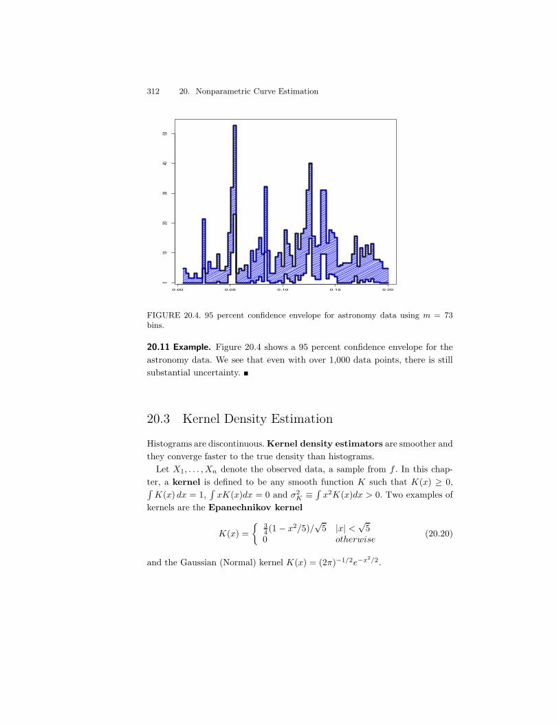
312 20. Nonparametric Curve Estimation
0.00 0.05 0.10 0.15 0.20
010
2030
4050
FIGURE 20.4. 95 percent confidence envelope for astronomy data using m = 73bins.
20.11 Example. Figure 20.4 shows a 95 percent confidence envelope for theastronomy data. We see that even with over 1,000 data points, there is stillsubstantial uncertainty. !
20.3 Kernel Density Estimation
Histograms are discontinuous. Kernel density estimators are smoother andthey converge faster to the true density than histograms.
Let X1, . . . , Xn denote the observed data, a sample from f . In this chap-ter, a kernel is defined to be any smooth function K such that K(x) * 0,8
K(x) dx = 1,8
xK(x)dx = 0 and #2K 0
8x2K(x)dx > 0. Two examples of
kernels are the Epanechnikov kernel
K(x) ='
34 (1 " x2/5)/
/5 |x| <
/5
0 otherwise(20.20)
and the Gaussian (Normal) kernel K(x) = (2&)$1/2e$x2/2.
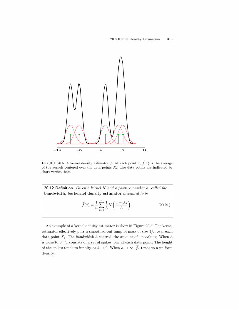
20.3 Kernel Density Estimation 313
!10 !5 0 5 10
FIGURE 20.5. A kernel density estimator 1f . At each point x, 1f(x) is the averageof the kernels centered over the data points Xi. The data points are indicated byshort vertical bars.
20.12 Definition. Given a kernel K and a positive number h, called thebandwidth, the kernel density estimator is defined to be
1f(x) =1n
n*
i=1
1h
K
-x"Xi
h
.. (20.21)
An example of a kernel density estimator is show in Figure 20.5. The kernelestimator e!ectively puts a smoothed-out lump of mass of size 1/n over eachdata point Xi. The bandwidth h controls the amount of smoothing. When h
is close to 0, 1fn consists of a set of spikes, one at each data point. The heightof the spikes tends to infinity as h) 0. When h)#, 1fn tends to a uniformdensity.
314 20. Nonparametric Curve Estimation
20.13 Example. Figure 20.6 shows kernel density estimators for the astron-omy data using three di!erent bandwidths. In each case we used a Gaussiankernel. The properly smoothed kernel density estimator in the top right panelshows similar structure as the histogram. However, it is easier to see the clus-ters with the kernel estimator. !
To construct a kernel density estimator, we need to choose a kernel K anda bandwidth h. It can be shown theoretically and empirically that the choiceof K is not crucial. 2 However, the choice of bandwidth h is very important.As with the histogram, we can make a theoretical statement about how therisk of the estimator depends on the bandwidth.
20.14 Theorem. Under weak assumptions on f and K,
R(f, 1fn) . 14#4
Kh4
9(f
""(x))2 +
8K2(x)dx
nh(20.22)
where #2K =
8x2K(x)dx. The optimal bandwidth is
h* =c$2/51 c1/5
2 c$1/53
n1/5(20.23)
where c1 =8
x2K(x)dx, c2 =8
K(x)2dx and c3 =8(f &&(x))2dx. With this
choice of bandwidth,R(f, 1fn) . c4
n4/5
for some constant c4 > 0.
Proof. Write Kh(x, X) = h$1K ((x "X)/h) and 1fn(x) = n$10
i Kh(x, Xi).Thus, E[ 1fn(x)] = E[Kh(x, X)] and V[ 1fn(x)] = n$1V[Kh(x, X)]. Now,
E[Kh(x, X)] =9
1h
K
-x" t
h
.f(t) dt
=9
K(u)f(x" hu) du
=9
K(u)Af(x) " hf
"(x) +
12f
""(x) + · · ·
Bdu
= f(x) +12h2f
""(x)9
u2K(u) du · · ·
since8
K(x) dx = 1 and8
xK(x) dx = 0. The bias is
E[Kh(x, X)]" f(x) . 12#2
kh2f""(x).
2It can be shown that the Epanechnikov kernel is optimal in the sense of giving smallestasymptotic mean squared error, but it is really the choice of bandwidth which is crucial.
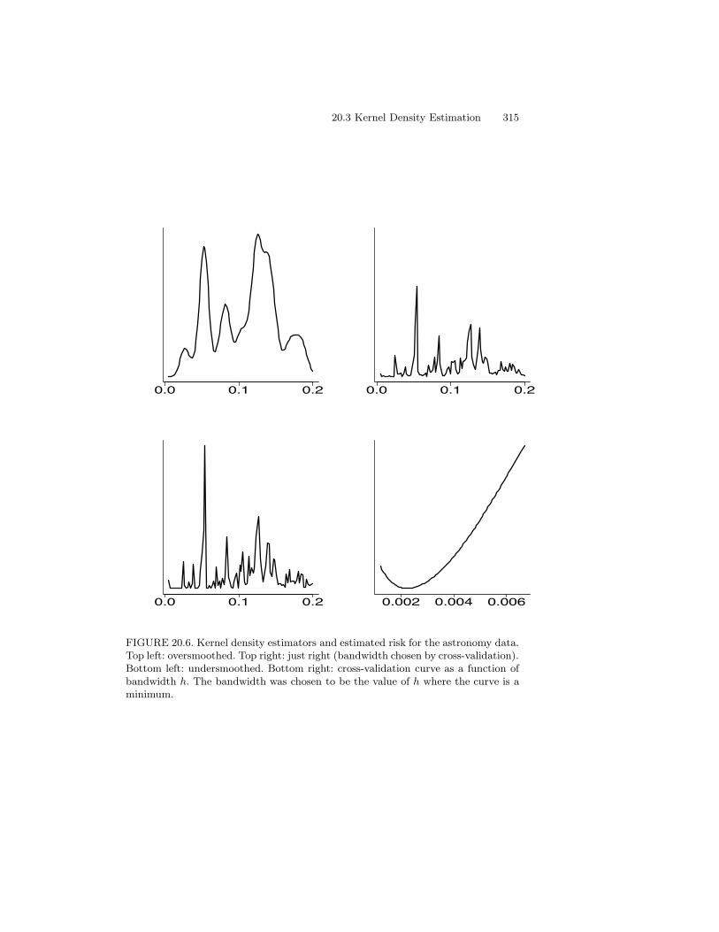
20.3 Kernel Density Estimation 315
0.0 0.1 0.2 0.0 0.1 0.2
0.0 0.1 0.2 0.002 0.004 0.006
FIGURE 20.6. Kernel density estimators and estimated risk for the astronomy data.Top left: oversmoothed. Top right: just right (bandwidth chosen by cross-validation).Bottom left: undersmoothed. Bottom right: cross-validation curve as a function ofbandwidth h. The bandwidth was chosen to be the value of h where the curve is aminimum.
316 20. Nonparametric Curve Estimation
By a similar calculation,
V[ 1fn(x)] . f(x)8
K2(x) dx
n hn.
The result follows from integrating the squared bias plus the variance. !
We see that kernel estimators converge at rate n$4/5 while histograms con-verge at the slower rate n$2/3. It can be shown that, under weak assumptions,there does not exist a nonparametric estimator that converges faster thann$4/5.
The expression for h* depends on the unknown density f which makesthe result of little practical use. As with the histograms, we shall use cross-validation to find a bandwidth. Thus, we estimate the risk (up to a constant)by
1J(h) =91f2(x)dz " 2
n
n*
i=1
1f$i(Xi) (20.24)
where 1f$i is the kernel density estimator after omitting the ith observation.
20.15 Theorem. For any h > 0,
E?1J(h)
@= E [J(h)] .
Also,
1J(h) . 1hn2
*
i
*
j
K*-
Xi "Xj
h
.+
2nh
K(0) (20.25)
where K*(x) = K(2)(x) " 2K(x) and K(2)(z) =8
K(z " y)K(y)dy. In par-ticular, if K is a N(0,1) Gaussian kernel then K(2)(z) is the N(0, 2) density.
We then choose the bandwidth hn that minimizes 1J(h).3 A justification forthis method is given by the following remarkable theorem due to Stone.
20.16 Theorem (Stone’s Theorem). Suppose that f is bounded. Let 1fh denotethe kernel estimator with bandwidth h and let hn denote the bandwidth chosenby cross-validation. Then,
8 +f(x)" 1fhn(x)
,2dx
infh
8 +f(x)" 1fh(x)
,2dx
P") 1. (20.26)
3For large data sets, 1f and (20.25) can be computed quickly using the fast Fourier transform.
20.3 Kernel Density Estimation 317
20.17 Example. The top right panel of Figure 20.6 is based on cross-validation.These data are rounded which problems for cross-validation. Specifically, itcauses the minimizer to be h = 0. To overcome this problem, we added asmall amount of random Normal noise to the data. The result is that 1J(h) isvery smooth with a well defined minimum. !
20.18 Remark. Do not assume that, if the estimator 1f is wiggly, then cross-validation has let you down. The eye is not a good judge of risk.
To construct confidence bands, we use something similar to histograms.Again, the confidence band is for the smoothed version,
fn = E( 1fn(x)) =9
1h
K
-x" u
h
.f(u) du,
of the true density f . 4 Assume the density is on an interval (a, b). The bandis
4n(x) = 1fn(x) " q se(x), un(x) = 1fn(x) + q se(x) (20.27)
where
se(x) =s(x)/
n,
s2(x) =1
n" 1
n*
i=1
(Yi(x) " Y n(x))2,
Yi(x) =1h
K
-x"Xi
h
.,
q = %$1
-1 + (1 " ))1/m
2
.,
m =b " a
"
where " is the width of the kernel. In case the kernel does not have finitewidth then we take " to be the e!ective width, that is, the range over whichthe kernel is non-negligible. In particular, we take " = 3h for the Normalkernel.
20.19 Example. Figure 20.7 shows approximate 95 percent confidence bandsfor the astronomy data. !
4This is a modified version of the band described in Chaudhuri and Marron (1999).
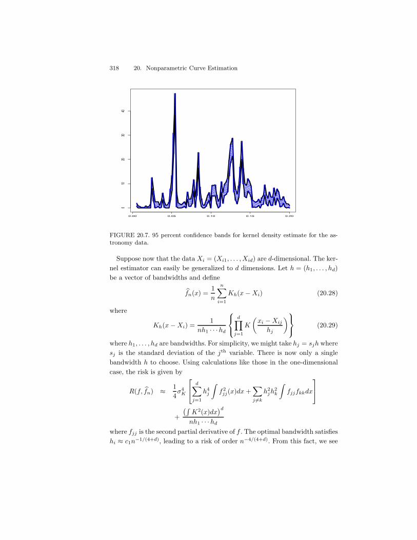
318 20. Nonparametric Curve Estimation
0.00 0.05 0.10 0.15 0.20
010
2030
40
FIGURE 20.7. 95 percent confidence bands for kernel density estimate for the as-tronomy data.
Suppose now that the data Xi = (Xi1, . . . , Xid) are d-dimensional. The ker-nel estimator can easily be generalized to d dimensions. Let h = (h1, . . . , hd)be a vector of bandwidths and define
1fn(x) =1n
n*
i=1
Kh(x "Xi) (20.28)
where
Kh(x"Xi) =1
nh1 · · ·hd
46
7
d/
j=1
K
-xi "Xij
hj
.KL
M (20.29)
where h1, . . . , hd are bandwidths. For simplicity, we might take hj = sjh wheresj is the standard deviation of the jth variable. There is now only a singlebandwidth h to choose. Using calculations like those in the one-dimensionalcase, the risk is given by
R(f, 1fn) . 14#4
K
N
Pd*
j=1
h4j
9f2
jj(x)dx +*
j .=k
h2jh
2k
9fjjfkkdx
Q
S
+;8
K2(x)dx<d
nh1 · · ·hd
where fjj is the second partial derivative of f . The optimal bandwidth satisfieshi . c1n$1/(4+d), leading to a risk of order n$4/(4+d). From this fact, we see
20.4 Nonparametric Regression 319
that the risk increases quickly with dimension, a problem usually called thecurse of dimensionality. To get a sense of how serious this problem is,consider the following table from Silverman (1986) which shows the samplesize required to ensure a relative mean squared error less than 0.1 at 0 whenthe density is multivariate normal and the optimal bandwidth is selected:
Dimension Sample Size1 42 193 674 2235 7686 27907 10,7008 43,7009 187,000
10 842,000
This is bad news indeed. It says that having 842,000 observations in a ten-dimensional problem is really like having 4 observations in a one-dimensionalproblem.
20.4 Nonparametric Regression
Consider pairs of points (x1, Y1), . . . , (xn, Yn) related by
Yi = r(xi) + -i (20.30)
where E(-i) = 0. We have written the xi’s in lower case since we will treatthem as fixed. We can do this since, in regression, it is only the mean of Y
conditional on x that we are interested in. We want to estimate the regressionfunction r(x) = E(Y |X = x).
There are many nonparametric regression estimators. Most involve esti-mating r(x) by taking some sort of weighted average of the Yi’s, giving higherweight to those points near x. A popular version is the Nadaraya-Watsonkernel estimator.
20.20 Definition. The Nadaraya-Watson kernel estimator is definedby
1r(x) =n*
i=1
wi(x)Yi (20.31)
320 20. Nonparametric Curve Estimation
where K is a kernel and the weights wi(x) are given by
wi(x) =K;
x$xih
<
0nj=1 K
+x$xj
h
, . (20.32)
The form of this estimator comes from first estimating the joint densityf(x, y) using kernel density estimation and then inserting the estimate intothe formula,
r(x) = E(Y |X = x) =9
yf(y|x)dy =8
yf(x, y)dy8f(x, y)dy
.
20.21 Theorem. Suppose that V(-i) = #2. The risk of the Nadaraya-Watsonkernel estimator is
R(1rn, r) . h4
4
-9x2K2(x)dx
.4 9 -r&&(x) + 2r&(x)
f &(x)f(x)
.2
dx
+9
#28
K2(x)dx
nhf(x)dx. (20.33)
The optimal bandwidth decreases at rate n$1/5 and with this choice the riskdecreases at rate n$4/5.
In practice, to choose the bandwidth h we minimize the cross validationscore
1J(h) =n*
i=1
(Yi " 1r$i(xi))2 (20.34)
where 1r$i is the estimator we get by omitting the ith variable. Fortunately,there is a shortcut formula for computing 1J .
20.22 Theorem. 1J can be written as
1J(h) =n*
i=1
(Yi " 1r(xi))21
(1" K(0)
0nj=1 K
+xi#xj
h
,
)2 . (20.35)
20.23 Example. Figures 20.8 shows cosmic microwave background (CMB)data from BOOMERaNG (Netterfield et al. (2002)), Maxima (Lee et al.(2001)), and DASI (Halverson et al. (2002))). The data consist of n pairs(x1, Y1), . . ., (xn, Yn) where xi is called the multipole moment and Yi is the
20.4 Nonparametric Regression 321
estimated power spectrum of the temperature fluctuations. What you are see-ing are sound waves in the cosmic microwave background radiation which isthe heat, left over from the big bang. If r(x) denotes the true power spectrum,then
Yi = r(xi) + -i
where -i is a random error with mean 0. The location and size of peaks inr(x) provides valuable clues about the behavior of the early universe. Figure20.8 shows the fit based on cross-validation as well as an undersmoothed andoversmoothed fit. The cross-validation fit shows the presence of three well-defined peaks, as predicted by the physics of the big bang. !
The procedure for finding confidence bands is similar to that for densityestimation. However, we first need to estimate #2. Suppose that the xi’s areordered. Assuming r(x) is smooth, we have r(xi+1)" r(xi) . 0 and hence
Yi+1 " Yi =Ar(xi+1) + -i+1
B"Ar(xi) + -i
B. -i+1 " -i
and hence
V(Yi+1 " Yi) . V(-i+1 " -i) = V(-i+1) + V(-i) = 2#2.
We can thus use the average of the n" 1 di!erences Yi+1"Yi to estimate #2.Hence, define
1#2 =1
2(n" 1)
n$1*
i=1
(Yi+1 " Yi)2. (20.36)
As with density estimate, the confidence band is for the smoothed versionrn(x) = E(1rn(x)) of the true regression function r.
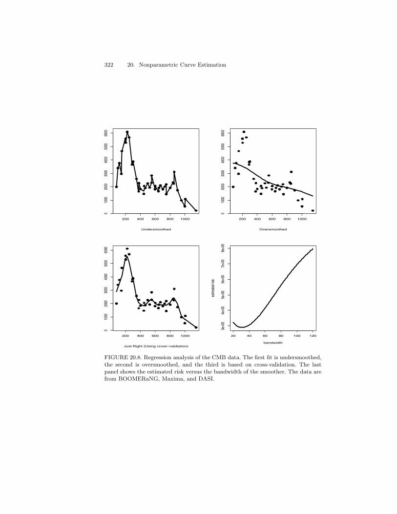
322 20. Nonparametric Curve Estimation
200 400 600 800 1000
010
0020
0030
0040
0050
0060
00
Undersmoothed
200 400 600 800 10000
1000
2000
3000
4000
5000
6000
Oversmoothed
200 400 600 800 1000
010
0020
0030
0040
0050
0060
00
Just Right (Using cross!valdiation)
20 40 60 80 100 120
3e+0
54e
+05
5e+0
56e
+05
7e+0
58e
+05
bandwidth
estima
ted ris
k
FIGURE 20.8. Regression analysis of the CMB data. The first fit is undersmoothed,the second is oversmoothed, and the third is based on cross-validation. The lastpanel shows the estimated risk versus the bandwidth of the smoother. The data arefrom BOOMERaNG, Maxima, and DASI.
20.4 Nonparametric Regression 323
Confidence Bands for Kernel Regression
An approximate 1" ) confidence band for rn(x) is
4n(x) = 1rn(x) " q 1se(x), un(x) = 1rn(x) + q 1se(x) (20.37)
where
1se(x) = 1#
\]] n*
i=1
w2i (x),
q = %$1
-1 + (1" ))1/m
2
.,
m =b" a
",
1# is defined in (20.36) and " is the width of the kernel. In case the kerneldoes not have finite width then we take " to be the e!ective width, thatis, the range over which the kernel is non-negligible. In particular, we take" = 3h for the Normal kernel.
20.24 Example. Figure 20.9 shows a 95 percent confidence envelope for theCMB data. We see that we are highly confident of the existence and positionof the first peak. We are more uncertain about the second and third peak.At the time of this writing, more accurate data are becoming available thatapparently provide sharper estimates of the second and third peak. !
The extension to multiple regressors X = (X1, . . . , Xp) is straightforward.As with kernel density estimation we just replace the kernel with a multivari-ate kernel. However, the same caveats about the curse of dimensionality apply.In some cases, we might consider putting some restrictions on the regressionfunction which will then reduce the curse of dimensionality. For example,additive regression is based on the model
Y =p*
j=1
rj(Xj) + -. (20.38)
Now we only need to fit p one-dimensional functions. The model can be en-riched by adding various interactions, for example,
Y =p*
j=1
rj(Xj) +*
j<k
rjk(XjXk) + -. (20.39)
Additive models are usually fit by an algorithm called backfitting.
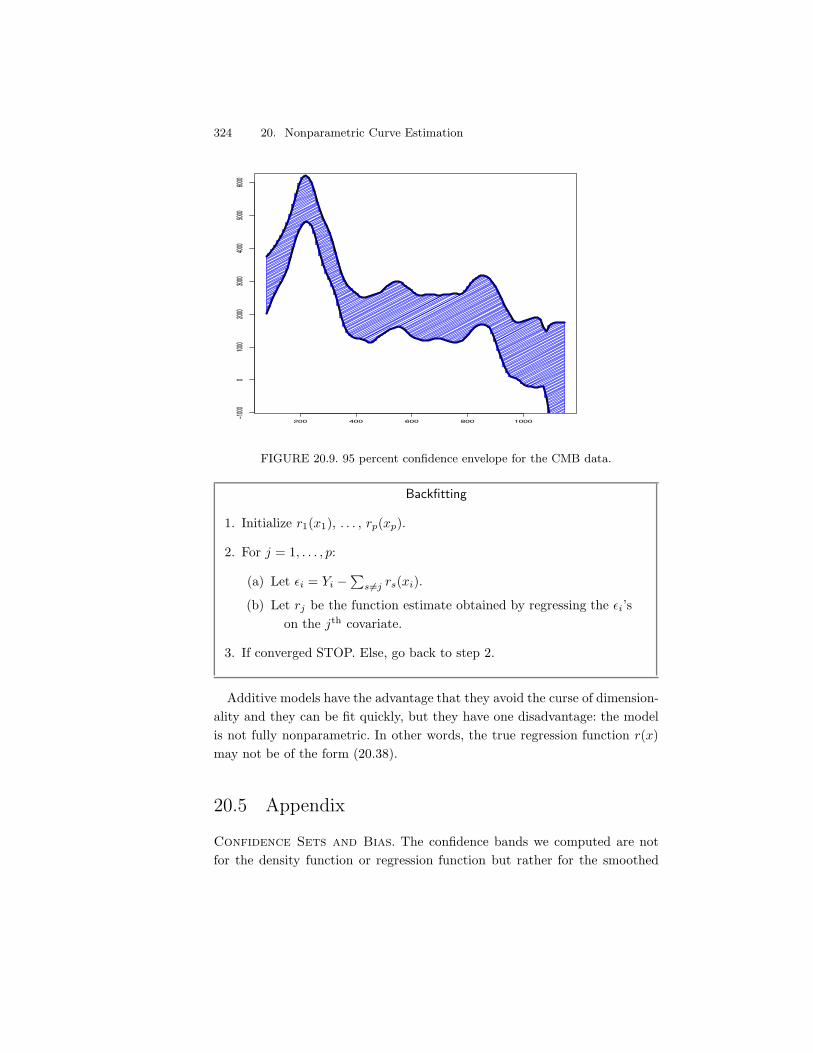
324 20. Nonparametric Curve Estimation
200 400 600 800 1000
!1000
0100
0200
0300
0400
0500
0600
0
FIGURE 20.9. 95 percent confidence envelope for the CMB data.
Backfitting
1. Initialize r1(x1), . . . , rp(xp).
2. For j = 1, . . . , p:
(a) Let -i = Yi "0
s.=j rs(xi).
(b) Let rj be the function estimate obtained by regressing the -i’son the jth covariate.
3. If converged STOP. Else, go back to step 2.
Additive models have the advantage that they avoid the curse of dimension-ality and they can be fit quickly, but they have one disadvantage: the modelis not fully nonparametric. In other words, the true regression function r(x)may not be of the form (20.38).
20.5 Appendix
Confidence Sets and Bias. The confidence bands we computed are notfor the density function or regression function but rather for the smoothed
20.6 Bibliographic Remarks 325
function. For example, the confidence band for a kernel density estimate withbandwidth h is a band for the function one gets by smoothing the true functionwith a kernel with the same bandwidth. Getting a confidence set for the truefunction is complicated for reasons we now explain.
Let 1fn(x) denote an estimate of the function f(x). Denote the mean andstandard deviation of 1fn(x) by fn(x) and sn(x). Then,
1fn(x) " f(x)sn(x)
=1fn(x)" fn(x)
sn(x)+
fn(x) " f(x)sn(x)
.
Typically, the first term converges to a standard Normal from which one de-rives confidence bands. The second term is the bias divided by the standarddeviation. In parametric inference, the bias is usually smaller than the stan-dard deviation of the estimator so this term goes to 0 as the sample sizeincreases. In nonparametric inference, optimal smoothing leads us to balancethe bias and the standard deviation. Thus the second term does not vanisheven with large sample sizes. This means that the confidence interval will notbe centered around the true function f .
20.6 Bibliographic Remarks
Two very good books on density estimation are Scott (1992) and Silverman(1986). The literature on nonparametric regression is very large. Two goodstarting points are Hardle (1990) and Loader (1999). The latter emphasizes aclass of techniques called local likelihood methods.
20.7 Exercises
1. Let X1, . . . , Xn ! f and let 1fn be the kernel density estimator using theboxcar kernel:
K(x) ='
1 " 12 < x < 1
20 otherwise.
(a) Show that
E( 1f(x)) =1h
9 x+(h/2)
x$(h/2)f(y)dy
and
V( 1f(x)) =1
nh2
N
P9 x+(h/2)
x$(h/2)f(y)dy "
(9 x+(h/2)
x$(h/2)f(y)dy
)2Q
S .
326 20. Nonparametric Curve Estimation
(b) Show that if h) 0 and nh)# as n)#, then 1fn(x) P") f(x).
2. Get the data on fragments of glass collected in forensic work from thebook website. Estimate the density of the first variable (refractive in-dex) using a histogram and use a kernel density estimator. Use cross-validation to choose the amount of smoothing. Experiment with di!erentbinwidths and bandwidths. Comment on the similarities and di!erences.Construct 95 percent confidence bands for your estimators.
3. Consider the data from question 2. Let Y be refractive index and letx be aluminum content (the fourth variable). Perform a nonparametricregression to fit the model Y = f(x)+-. Use cross-validation to estimatethe bandwidth. Construct 95 percent confidence bands for your estimate.
4. Prove Lemma 20.1.
5. Prove Theorem 20.3.
6. Prove Theorem 20.7.
7. Prove Theorem 20.15.
8. Consider regression data (x1, Y1), . . . , (xn, Yn). Suppose that 0 , xi , 1for all i. Define bins Bj as in equation (20.7). For x $ Bj define
1rn(x) = Y j
where Y j is the mean of all the Yi’s corresponding to those xi’s in Bj .Find the approximate risk of this estimator. From this expression forthe risk, find the optimal bandwidth. At what rate does the risk go tozero?
9. Show that with suitable smoothness assumptions on r(x), 1#2 in equation(20.36) is a consistent estimator of #2.
10. Prove Theorem 20.22.
This is page 327Printer: Opaque this
21Smoothing Using Orthogonal Functions
In this chapter we will study an approach to nonparametric curve estima-tion based on orthogonal functions. We begin with a brief introduction tothe theory of orthogonal functions, then we turn to density estimation andregression.
21.1 Orthogonal Functions and L2 Spaces
Let v = (v1, v2, v3) denote a three-dimensional vector, that is, a list of threereal numbers. Let V denote the set of all such vectors. If a is a scalar (anumber) and v is a vector, we define av = (av1, av2, av3). The sum of vectorsv and w is defined by v+w = (v1 +w1, v2 +w2, v3 +w3). The inner productbetween two vectors v and w is defined by 6v, w7 =
03i=1 viwi. The norm
(or length) of a vector v is defined by
||v|| =36v, v7 =
\]] 3*
i=1
v2i . (21.1)
Two vectors are orthogonal (or perpendicular) if 6v, w7 = 0. A set ofvectors are orthogonal if each pair in the set is orthogonal. A vector is normalif ||v|| = 1.
328 21. Smoothing Using Orthogonal Functions
Let '1 = (1, 0, 0), '2 = (0, 1, 0), '3 = (0, 0, 1). These vectors are said to bean orthonormal basis for V since they have the following properties:(i) they are orthogonal;(ii) they are normal;(iii) they form a basis for V , which means that any v $ V can be written as alinear combination of '1, '2, '3:
v =3*
j=1
(j'j where (j = 6'j , v7. (21.2)
For example, if v = (12, 3, 4) then v = 12'1 + 3'2 + 4'3. There are otherorthonormal bases for V , for example,
,1 =-
1/3,
1/3,
1/3
., ,2 =
-1/2," 1/
2, 0.
, ,3 =-
1/6,
1/6," 2/
6
..
You can check that these three vectors also form an orthonormal basis for V .Again, if v is any vector then we can write
v =3*
j=1
(j,j where (j = 6,j , v7.
For example, if v = (12, 3, 4) then
v = 10.97,1 + 6.36,2 + 2.86,3.
Now we make the leap from vectors to functions. Basically, we just replacevectors with functions and sums with integrals. Let L2(a, b) denote all func-tions defined on the interval [a, b] such that
8 ba f(x)2dx <#:
L2(a, b) =
:f : [a, b]) R,
9 b
af(x)2dx <#
Y. (21.3)
We sometimes write L2 instead of L2(a, b). The inner product between twofunctions f, g $ L2 is defined by
8f(x)g(x)dx. The norm of f is
||f || =
T9f(x)2dx. (21.4)
Two functions are orthogonal if8
f(x)g(x)dx = 0. A function is normal if||f || = 1.
A sequence of functions '1,'2,'3, . . . is orthonormal if8'2
j (x)dx = 1 foreach j and
8'i(x)'j(x)dx = 0 for i (= j. An orthonormal sequence is com-
plete if the only function that is orthogonal to each 'j is the zero function.
21.1 Orthogonal Functions and L2 Spaces 329
In this case, the functions '1,'2,'3, . . . form in basis, meaning that if f $ L2
then f can be written as1
f(x) =!*
j=1
(j'j(x), where (j =9 b
af(x)'j(x)dx. (21.5)
A useful result is Parseval’s relation which says that
||f ||2 09
f2(x) dx =!*
j=1
(2j 0 ||(||2 (21.6)
where ( = ((1,(2, . . .).
21.1 Example. An example of an orthonormal basis for L2(0, 1) is the cosinebasis defined as follows. Let '0(x) = 1 and for j * 1 define
'j(x) =/
2 cos(j&x). (21.7)
The first six functions are plotted in Figure 21.1. !
21.2 Example. Let
f(x) =3
x(1 " x) sin-
2.1&(x + .05)
.
which is called the “doppler function.” Figure 21.2 shows f (top left) and itsapproximation
fJ(x) =J*
j=1
(j'j(x)
with J equal to 5 (top right), 20 (bottom left), and 200 (bottom right).As J increases we see that fJ(x) gets closer to f(x). The coe#cients (j =8 10 f(x)'j(x)dx were computed numerically. !
21.3 Example. The Legendre polynomials on ["1, 1] are defined by
Pj(x) =1
2jj!dj
dxj(x2 " 1)j , j = 0, 1, 2, . . . (21.8)
It can be shown that these functions are complete and orthogonal and that9 1
$1P 2
j (x)dx =2
2j + 1. (21.9)
1The equality in the displayed equation means that8
(f(x)"fn(x))2dx $ 0 where fn(x) =0nj=1 βjφj(x).
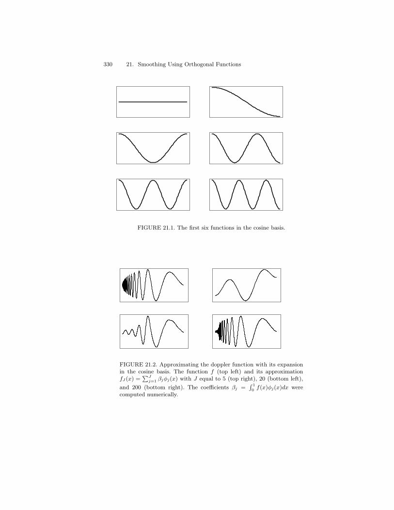
330 21. Smoothing Using Orthogonal Functions
FIGURE 21.1. The first six functions in the cosine basis.
FIGURE 21.2. Approximating the doppler function with its expansionin the cosine basis. The function f (top left) and its approximationfJ (x) =
0Jj=1 "j%j(x) with J equal to 5 (top right), 20 (bottom left),
and 200 (bottom right). The coe#cients "j =8 10
f(x)%j(x)dx werecomputed numerically.
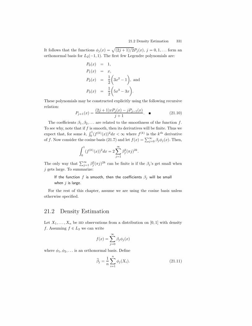
21.2 Density Estimation 331
It follows that the functions 'j(x) =3
(2j + 1)/2Pj(x), j = 0, 1, . . . form anorthonormal basis for L2("1, 1). The first few Legendre polynomials are:
P0(x) = 1,
P1(x) = x,
P2(x) =12
-3x2 " 1
., and
P3(x) =12
-5x3 " 3x
..
These polynomials may be constructed explicitly using the following recursiverelation:
Pj+1(x) =(2j + 1)xPj(x) " jPj$1(x)
j + 1. ! (21.10)
The coe#cients (1,(2, . . . are related to the smoothness of the function f .To see why, note that if f is smooth, then its derivatives will be finite. Thus weexpect that, for some k,
8 10 (f (k)(x))2dx <# where f (k) is the kth derivative
of f . Now consider the cosine basis (21.7) and let f(x) =0!
j=0 (j'j(x). Then,9 1
0(f (k)(x))2dx = 2
!*
j=1
(2j (&j)2k.
The only way that0!
j=1 (2j (&j)2k can be finite is if the (j ’s get small when
j gets large. To summarize:
If the function f is smooth, then the coe"cients (j will be small
when j is large.
For the rest of this chapter, assume we are using the cosine basis unlessotherwise specified.
21.2 Density Estimation
Let X1, . . . , Xn be iid observations from a distribution on [0, 1] with densityf . Assuming f $ L2 we can write
f(x) =!*
j=0
(j'j(x)
where '1,'2, . . . is an orthonormal basis. Define
1(j =1n
n*
i=1
'j(Xi). (21.11)
332 21. Smoothing Using Orthogonal Functions
21.4 Theorem. The mean and variance of 1(j are
E+1(j
,= (j, V
+1(j
,=#2
j
n(21.12)
where#2
j = V('j(Xi)) =9
('j(x)" (j)2f(x)dx. (21.13)
Proof. The mean is
E+1(j
,=
1n
n*
i=1
E ('j(Xi))
= E ('j(X1))
=9'j(x)f(x)dx = (j .
The calculation for the variance is similar. !
Hence, 1(j is an unbiased estimate of (j . It is tempting to estimate f by0!j=11(j'j(x) but this turns out to have a very high variance. Instead, consider
the estimator
1f(x) =J*
j=1
1(j'j(x). (21.14)
The number of terms J is a smoothing parameter. Increasing J will decreasebias while increasing variance. For technical reasons, we restrict J to lie inthe range
1 , J , p
where p = p(n) =/
n. To emphasize the dependence of the risk function onJ , we write the risk function as R(J).
21.5 Theorem. The risk of 1f is
R(J) =J*
j=1
#2j
n+
!*
j=J+1
(2j . (21.15)
An estimate of the risk is
1R(J) =J*
j=1
1#2j
n+
p*
j=J+1
(1(2j "
1#2j
n
)
+
(21.16)
where a+ = max{a, 0} and
1#2j =
1n" 1
n*
i=1
+'j(Xi)" 1(j
,2. (21.17)
21.2 Density Estimation 333
To motivate this estimator, note that 1#2j is an unbiased estimate of #2
j and1(2j " 1#2
j is an unbiased estimator of (2j . We take the positive part of the latter
term since we know that (2j cannot be negative. We now choose 1 , 1J , p to
minimize 1R( 1f, f). Here is a summary:
Summary of Orthogonal Function Density Estimation
1. Let1(j =
1n
n*
i=1
'j(Xi).
2. Choose 1J to minimize 1R(J) over 1 , J , p =/
n where 1R is given inequation (21.16).
3. Let
1f(x) =1J*
j=1
1(j'j(x).
The estimator 1fn can be negative. If we are interested in exploring theshape of f , this is not a problem. However, if we need our estimate to be aprobability density function, we can truncate the estimate and then normalizeit. That is, we take 1f* = max{ 1fn(x), 0}/
8 10 max{ 1fn(u), 0}du.
Now let us construct a confidence band for f . Suppose we estimate f usingJ orthogonal functions. We are essentially estimating fJ(x) =
0Jj=1 (j'j(x)
not the true density f(x) =0!
j=1 (j'j(x). Thus, the confidence band shouldbe regarded as a band for fJ(x).
21.6 Theorem. An approximate 1 " ) confidence band for fJ is (4(x), u(x))where
4(x) = 1fn(x) " c, u(x) = 1fn(x) + c (21.18)
where
c = K2
TJ!2
J,#
n(21.19)
andK = max
1%j%Jmax
x|'j(x)|.
For the cosine basis, K =/
2.
Proof. Here is an outline of the proof. Let L =0J
j=1(1(j " (j)2. By thecentral limit theorem, 1(j . N((j ,#2
j /n). Hence, 1(j . (j + #j-j//
n where
334 21. Smoothing Using Orthogonal Functions
-j ! N(0, 1), and therefore
L . 1n
J*
j=1
#2j -
2j ,
K2
n
J*
j=1
-2jd=
K2
n!2
J . (21.20)
Thus we have, approximately, that
P-
L >K2
n!2
J,#
., P
-K2
n!2
J >K2
n!2
J,#
.= ).
Also,
maxx
| 1fJ(x)" fJ(x)| , maxx
J*
j=1
|'j(x)| |1(j " (j |
, KJ*
j=1
|1(j " (j|
,/
J K
\]] J*
j=1
(1(j " (j)2
=/
J K/
L
where the third inequality is from the Cauchy-Schwartz inequality (Theorem4.8). So,
P
E
Gmaxx
| 1fJ (x)" fJ(x)| > K2
TJ!2
J,#
n
H
J , P
E
G/
J K/
L > K2
TJ!2
J,#
n
H
J
= P
E
G/
L > K
T!2
J,#
n
H
J
= P(
L >K2!2
J,#
n
)
, ). !
21.7 Example. Let
f(x) =56'(x; 0, 1) +
16
5*
j=1
'(x; µj , .1)
where '(x; µ,#) denotes a Normal density with mean µ and standard deviation#, and (µ1, . . . , µ5) = ("1,"1/2, 0, 1/2, 1). Marron and Wand (1992) call this
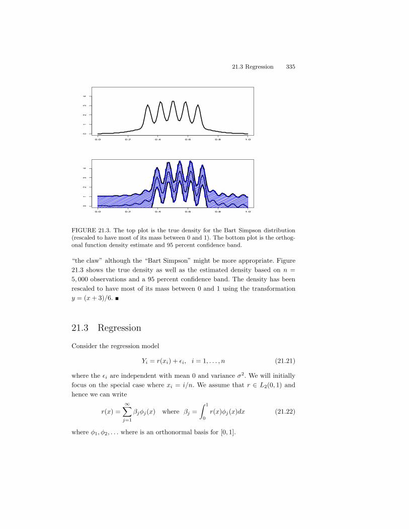
21.3 Regression 335
0.0 0.2 0.4 0.6 0.8 1.0
01
23
4
0.0 0.2 0.4 0.6 0.8 1.0
01
23
4
FIGURE 21.3. The top plot is the true density for the Bart Simpson distribution(rescaled to have most of its mass between 0 and 1). The bottom plot is the orthog-onal function density estimate and 95 percent confidence band.
“the claw” although the “Bart Simpson” might be more appropriate. Figure21.3 shows the true density as well as the estimated density based on n =5, 000 observations and a 95 percent confidence band. The density has beenrescaled to have most of its mass between 0 and 1 using the transformationy = (x + 3)/6. !
21.3 Regression
Consider the regression model
Yi = r(xi) + -i, i = 1, . . . , n (21.21)
where the -i are independent with mean 0 and variance #2. We will initiallyfocus on the special case where xi = i/n. We assume that r $ L2(0, 1) andhence we can write
r(x) =!*
j=1
(j'j(x) where (j =9 1
0r(x)'j(x)dx (21.22)
where '1,'2, . . . where is an orthonormal basis for [0, 1].
336 21. Smoothing Using Orthogonal Functions
Define1(j =
1n
n*
i=1
Yi 'j(xi), j = 1, 2, . . . (21.23)
Since 1(j is an average, the central limit theorem tells us that 1(j will beapproximately Normally distributed.
21.8 Theorem.
1(j . N
-(j ,
#2
n
.. (21.24)
Proof. The mean of 1(j is
E(1(j) =1n
n*
i=1
E(Yi)'j(xi) =1n
n*
i=1
r(xi)'j(xi)
.9
r(x)'j (x)dx = (j
where the approximate equality follows from the definition of a Riemann in-tegral:
0i )nh(xi))
8 10 h(x)dx where )n = 1/n. The variance is
V(1(j) =1n2
n*
i=1
V(Yi)'2j (xi)
=#2
n2
n*
i=1
'2j(xi) =
#2
n
1n
n*
i=1
'2j(xi)
. #2
n
9'2
j(x)dx =#2
n
since8'2
j (x)dx = 1. !
Let
1r(x) =J*
j=1
1(j'j(x),
and letR(J) = E
9(r(x) " 1r(x))2 dx
be the risk of the estimator.
21.9 Theorem. The risk R(J) of the estimator 1rn(x) =0J
j=11(j'j(x) is
R(J) =J#2
n+
!*
j=J+1
(2j . (21.25)
21.3 Regression 337
To estimate for #2 = V(-i) we use
1#2 =n
k
n*
i=n$k+1
1(2j (21.26)
where k = n/4. To motivate this estimator, recall that if f is smooth, then(j . 0 for large j. So, for j * k, 1(j . N(0,#2/n) and thus, 1(j . #Zj/
/n for
for j * k, where Zj ! N(0, 1). Therefore,
1#2 =n
k
n*
i=n$k+1
1(2j .
n
k
n*
i=n$k+1
-#/n1(j
.2
=#2
k
n*
i=n$k+1
1(2j =
#2
k!2
k
since a sum of k Normals has a !2k distribution. Now E(!2
k) = k and henceE(1#2) . #2. Also, V(!2
k) = 2k and hence V(1#2) . (#4/k2)(2k) = (2#4/k)) 0as n ) #. Thus we expect 1#2 to be a consistent estimator of #2. There isnothing special about the choice k = n/4. Any k that increases with n at anappropriate rate will su#ce.
We estimate the risk with
1R(J) = J1#2
n+
n*
j=J+1
-1(2j "
1#2
n
.
+
. (21.27)
21.10 Example. Figure 21.4 shows the doppler function f and n = 2, 048observations generated from the model
Yi = r(xi) + -i
where xi = i/n, -i ! N(0, (.1)2). The figure shows the data and the estimatedfunction. The estimate was based on 1J = 234 terms. !
We are now ready to give a complete description of the method.
Orthogonal Series Regression Estimator
1. Let1(j =
1n
n*
i=1
Yi'j(xi), j = 1, . . . , n.
2. Let
1#2 =n
k
n*
i=n$k+1
1(2j (21.28)
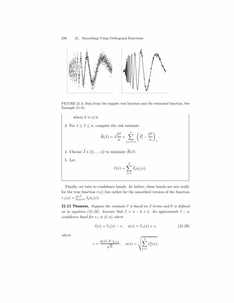
338 21. Smoothing Using Orthogonal Functions
FIGURE 21.4. Data from the doppler test function and the estimated function. SeeExample 21.10.
where k . n/4.
3. For 1 , J , n, compute the risk estimate
1R(J) = J1#2
n+
n*
j=J+1
-1(2j "
1#2
n
.
+
.
4. Choose 1J $ {1, . . . n} to minimize 1R(J).
5. Let
1r(x) =1J*
j=1
1(j'j(x).
Finally, we turn to confidence bands. As before, these bands are not reallyfor the true function r(x) but rather for the smoothed version of the functionrJ (x) =
01Jj=1 (j'j(x).
21.11 Theorem. Suppose the estimate 1r is based on J terms and 1# is definedas in equation (21.28). Assume that J < n " k + 1. An approximate 1 " )confidence band for rJ is (4, u) where
4(x) = 1rn(x) " c, u(x) = 1rn(x) + c, (21.29)
where
c =a(x) 1# !J,#/
n, a(x) =
\]] J*
j=1
'2j (x),
21.3 Regression 339
and 1# is given in equation (21.28).
Proof. Let L =0J
j=1(1(j " (j)2. By the central limit theorem, 1(j .N((j ,#2/n). Hence, 1(j . (j + #-j/
/n where -j ! N(0, 1) and therefore
L . #2
n
J*
j=1
-2jd=#2
n!2
J .
Thus,
P-
L >#2
n!2
J,#
.= P
-#2
n!2
J >#2
n!2
J,#
.= ).
Also,
|1r(x) " rJ(x)| ,J*
j=1
|'j(x)| |1(j " (j |
,
\]] J*
j=1
'2j (x)
\]] J*
j=1
(1(j " (2j )
, a(x)/
L
by the Cauchy-Schwartz inequality (Theorem 4.8). So,
P(
maxx
| 1fJ(x) " f(x)|a(x)
>1#!J,#/
n
), P
-/L >
1#!J,#/n
.
= )
and the result follows. !
21.12 Example. Figure 21.5 shows the confidence envelope for the dopplersignal. The first plot is based on J = 234 (the value of J that minimizes theestimated risk). The second is based on J = 45 .
/n. Larger J yields a higher
resolution estimator at the cost of large confidence bands. Smaller J yields alower resolution estimator but has tighter confidence bands. !
So far, we have assumed that the xi’s are of the form {1/n, 2/n, . . . , 1}.If the xi’s are on interval [a, b], then we can rescale them so that are in theinterval [0, 1]. If the xi’s are not equally spaced, the methods we have discussedstill apply so long as the xi’s “fill out” the interval [0,1] in such a way so as tonot be too clumped together. If we want to treat the xi’s as random insteadof fixed, then the method needs significant modifications which we shall notdeal with here.
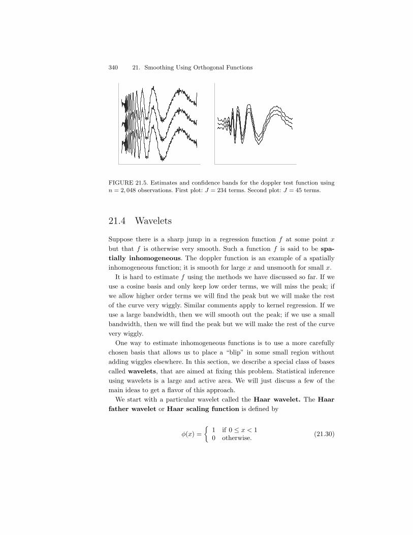
340 21. Smoothing Using Orthogonal Functions
FIGURE 21.5. Estimates and confidence bands for the doppler test function usingn = 2, 048 observations. First plot: J = 234 terms. Second plot: J = 45 terms.
21.4 Wavelets
Suppose there is a sharp jump in a regression function f at some point x
but that f is otherwise very smooth. Such a function f is said to be spa-tially inhomogeneous. The doppler function is an example of a spatiallyinhomogeneous function; it is smooth for large x and unsmooth for small x.
It is hard to estimate f using the methods we have discussed so far. If weuse a cosine basis and only keep low order terms, we will miss the peak; ifwe allow higher order terms we will find the peak but we will make the restof the curve very wiggly. Similar comments apply to kernel regression. If weuse a large bandwidth, then we will smooth out the peak; if we use a smallbandwidth, then we will find the peak but we will make the rest of the curvevery wiggly.
One way to estimate inhomogeneous functions is to use a more carefullychosen basis that allows us to place a “blip” in some small region withoutadding wiggles elsewhere. In this section, we describe a special class of basescalled wavelets, that are aimed at fixing this problem. Statistical inferenceusing wavelets is a large and active area. We will just discuss a few of themain ideas to get a flavor of this approach.
We start with a particular wavelet called the Haar wavelet. The Haarfather wavelet or Haar scaling function is defined by
'(x) ='
1 if 0 , x < 10 otherwise. (21.30)
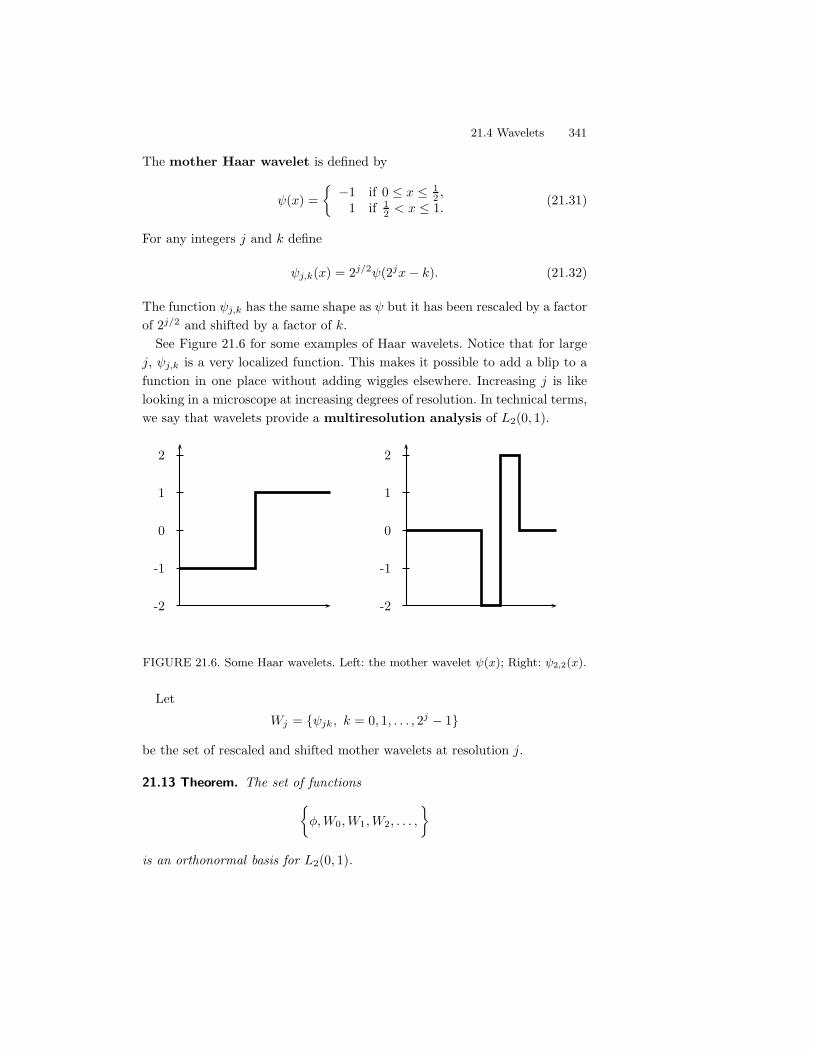
21.4 Wavelets 341
The mother Haar wavelet is defined by
,(x) ='"1 if 0 , x , 1
2 ,1 if 1
2 < x , 1.(21.31)
For any integers j and k define
,j,k(x) = 2j/2,(2jx" k). (21.32)
The function ,j,k has the same shape as , but it has been rescaled by a factorof 2j/2 and shifted by a factor of k.
See Figure 21.6 for some examples of Haar wavelets. Notice that for largej, ,j,k is a very localized function. This makes it possible to add a blip to afunction in one place without adding wiggles elsewhere. Increasing j is likelooking in a microscope at increasing degrees of resolution. In technical terms,we say that wavelets provide a multiresolution analysis of L2(0, 1).
-2
-1
0
1
2
-2
-1
0
1
2
FIGURE 21.6. Some Haar wavelets. Left: the mother wavelet &(x); Right: &2,2(x).
Let
Wj = {,jk, k = 0, 1, . . . , 2j " 1}
be the set of rescaled and shifted mother wavelets at resolution j.
21.13 Theorem. The set of functions'', W0, W1, W2, . . . ,
2
is an orthonormal basis for L2(0, 1).
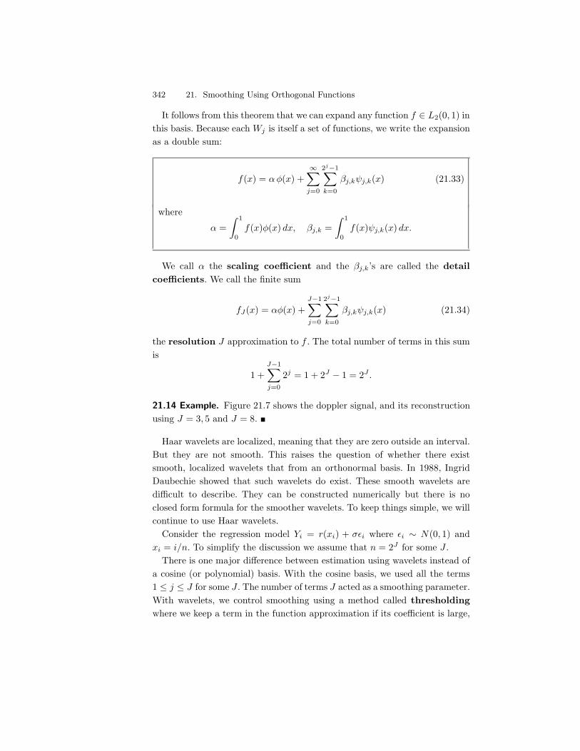
342 21. Smoothing Using Orthogonal Functions
It follows from this theorem that we can expand any function f $ L2(0, 1) inthis basis. Because each Wj is itself a set of functions, we write the expansionas a double sum:
f(x) = )'(x) +!*
j=0
2j$1*
k=0
(j,k,j,k(x) (21.33)
where
) =9 1
0f(x)'(x) dx, (j,k =
9 1
0f(x),j,k(x) dx.
We call ) the scaling coe!cient and the (j,k’s are called the detailcoe!cients. We call the finite sum
fJ(x) = )'(x) +J$1*
j=0
2j$1*
k=0
(j,k,j,k(x) (21.34)
the resolution J approximation to f . The total number of terms in this sumis
1 +J$1*
j=0
2j = 1 + 2J " 1 = 2J .
21.14 Example. Figure 21.7 shows the doppler signal, and its reconstructionusing J = 3, 5 and J = 8. !
Haar wavelets are localized, meaning that they are zero outside an interval.But they are not smooth. This raises the question of whether there existsmooth, localized wavelets that from an orthonormal basis. In 1988, IngridDaubechie showed that such wavelets do exist. These smooth wavelets aredi#cult to describe. They can be constructed numerically but there is noclosed form formula for the smoother wavelets. To keep things simple, we willcontinue to use Haar wavelets.
Consider the regression model Yi = r(xi) + #-i where -i ! N(0, 1) andxi = i/n. To simplify the discussion we assume that n = 2J for some J .
There is one major di!erence between estimation using wavelets instead ofa cosine (or polynomial) basis. With the cosine basis, we used all the terms1 , j , J for some J . The number of terms J acted as a smoothing parameter.With wavelets, we control smoothing using a method called thresholdingwhere we keep a term in the function approximation if its coe#cient is large,
21.4 Wavelets 343
0.0 0.2 0.4 0.6 0.8 1.0
!0.4
!0.2
0.00.2
0.4
x
f
0.0 0.2 0.4 0.6 0.8 1.0
!0.4
!0.2
0.00.2
0.4
0.0 0.2 0.4 0.6 0.8 1.0
!0.4
!0.2
0.00.2
0.4
0.0 0.2 0.4 0.6 0.8 1.0
!0.4
!0.2
0.00.2
0.4
FIGURE 21.7. The doppler signal and its reconstructionfJ (x) = #%(x) +
0J!1j=0
0k "j,k&j,k(x) based on J = 3, J = 5, and J = 8.
otherwise, we throw out that term. There are many versions of thresholding.The simplest is called hard, universal thresholding. Let J = log2(n) and define
1) =1n
*
i
'k(xi)Yi and Dj,k =1n
*
i
,j,k(xi)Yi (21.35)
for 0 , j , J " 1.
Haar Wavelet Regression
1. Compute 1) and Dj,k as in (21.35), for 0 , j , J " 1.
2. Estimate #; see (21.37).
3. Apply universal thresholding:
1(j,k =
:Dj,k if |Dj,k| > 1#
V2 log n
n
0 otherwise.
Y(21.36)
4. Set 1f(x) = 1)'(x) +0J$1
j=j0
02j$1k=0
1(j,k,j,k(x).
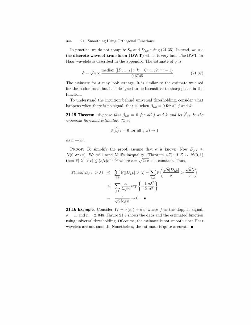
344 21. Smoothing Using Orthogonal Functions
In practice, we do not compute Sk and Dj,k using (21.35). Instead, we usethe discrete wavelet transform (DWT) which is very fast. The DWT forHaar wavelets is described in the appendix. The estimate of # is
1# =/
n-median
;|DJ$1,k| : k = 0, . . . , 2J$1 " 1
<
0.6745. (21.37)
The estimate for # may look strange. It is similar to the estimate we usedfor the cosine basis but it is designed to be insensitive to sharp peaks in thefunction.
To understand the intuition behind universal thresholding, consider whathappens when there is no signal, that is, when (j,k = 0 for all j and k.
21.15 Theorem. Suppose that (j,k = 0 for all j and k and let 1(j,k be theuniversal threshold estimator. Then
P(1(j,k = 0 for all j, k)) 1
as n)#.
Proof. To simplify the proof, assume that # is known. Now Dj,k .N(0,#2/n). We will need Mill’s inequality (Theorem 4.7): if Z ! N(0, 1)then P(|Z| > t) , (c/t)e$t2/2 where c =
32/& is a constant. Thus,
P(max |Dj,k| > %) ,*
j,k
P(|Dj,k| > %) =*
j,k
P-/
n|Dj,k|#
>
/n%
#
.
,*
j,k
c#
%/
nexp'"1
2n%2
#2
2
=c/
2 logn) 0. !
21.16 Example. Consider Yi = r(xi) + #-i where f is the doppler signal,# = .1 and n = 2, 048. Figure 21.8 shows the data and the estimated functionusing universal thresholding. Of course, the estimate is not smooth since Haarwavelets are not smooth. Nonetheless, the estimate is quite accurate. !
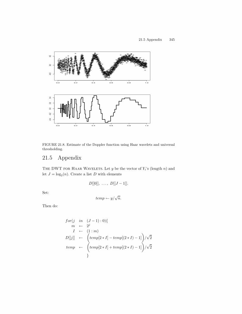
21.5 Appendix 345
0.0 0.2 0.4 0.6 0.8 1.0
!0.5
0.00.5
0.0 0.2 0.4 0.6 0.8 1.0
!0.4
!0.2
0.00.2
0.4
FIGURE 21.8. Estimate of the Doppler function using Haar wavelets and universalthresholding.
21.5 Appendix
The DWT for Haar Wavelets. Let y be the vector of Yi’s (length n) andlet J = log2(n). Create a list D with elements
D[[0]], . . . , D[[J " 1]].
Set:temp4 y/
/n.
Then do:
for(j in (J " 1) : 0){m 4 2j
I 4 (1 : m)
D[[j]] 4-
temp[2 8 I]" temp[(2 8 I)" 1].
//
2
temp 4-
temp[2 8 I] + temp[(2 8 I)" 1].
//
2
}
346 21. Smoothing Using Orthogonal Functions
21.6 Bibliographic Remarks
Efromovich (1999) is a reference for orthogonal function methods. See alsoBeran (2000) and Beran and Dumbgen (1998). An introduction to wavelets isgiven in Ogden (1997). A more advanced treatment can be found in Hardleet al. (1998). The theory of statistical estimation using wavelets has beendeveloped by many authors, especially David Donoho and Ian Johnstone. SeeDonoho and Johnstone (1994), Donoho and Johnstone (1995), Donoho et al.(1995), and Donoho and Johnstone (1998).
21.7 Exercises
1. Prove Theorem 21.5.
2. Prove Theorem 21.9.
3. Let
,1 =-
1/3,
1/3,
1/3
., ,2 =
-1/2," 1/
2, 0.
, ,3 =-
1/6,
1/6," 2/
6
..
Show that these vectors have norm 1 and are orthogonal.
4. Prove Parseval’s relation equation (21.6).
5. Plot the first five Legendre polynomials. Verify, numerically, that theyare orthonormal.
6. Expand the following functions in the cosine basis on [0, 1]. For (a)and (b), find the coe#cients (j analytically. For (c) and (d), find thecoe#cients (j numerically, i.e.
(j =9 1
0f(x)'j(x) . 1
N
N*
r=1
f+ r
N
,'j
+ r
N
,
for some large integer N . Then plot the partial sum0n
j=1 (j'j(x) forincreasing values of n.
(a) f(x) =/
2 cos(3&x).
(b) f(x) = sin(&x).
(c) f(x) =011
j=1 hjK(x"tj) where K(t) = (1+sign(t))/2, sign(x) = "1if x < 0, sign(x) = 0 if x = 0, sign(x) = 1 if x > 0,
21.7 Exercises 347
(tj) = (.1, .13, .15, .23, .25, .40, .44, .65, .76, .78, .81),
(hj) = (4,"5, 3,"4, 5,"4.2, 2.1, 4.3,"3.1, 2.1,"4.2).
(d) f =3
x(1" x) sin+
2.1-(x+.05)
,.
7. Consider the glass fragments data from the book’s website. Let Y berefractive index and let X be aluminum content (the fourth variable).
(a) Do a nonparametric regression to fit the model Y = f(x) + - usingthe cosine basis method. The data are not on a regular grid. Ignore thiswhen estimating the function. (But do sort the data first according tox.) Provide a function estimate, an estimate of the risk, and a confidenceband.
(b) Use the wavelet method to estimate f .
8. Show that the Haar wavelets are orthonormal.
9. Consider again the doppler signal:
f(x) =3
x(1 " x) sin-
2.1&x + 0.05
..
Let n = 1, 024, # = 0.1, and let (x1, . . . , xn) = (1/n, . . . , 1). Generatedata
Yi = f(xi) + #-i
where -i ! N(0, 1).
(a) Fit the curve using the cosine basis method. Plot the function esti-mate and confidence band for J = 10, 20, . . . , 100.
(b) Use Haar wavelets to fit the curve.
10. (Haar density Estimation.) Let X1, . . . , Xn ! f for some density f on[0, 1]. Let’s consider constructing a wavelet histogram. Let ' and , bethe Haar father and mother wavelet. Write
f(x) . '(x) +J$1*
j=0
2j$1*
k=0
(j,k,j,k(x)
where J . log2(n). Let
1(j,k =1n
n*
i=1
,j,k(Xi).
348 21. Smoothing Using Orthogonal Functions
(a) Show that 1(j,k is an unbiased estimate of (j,k.
(b) Define the Haar histogram
1f(x) = '(x) +B*
j=0
2j$1*
k=0
1(j,k,j,k(x)
for 0 , B , J " 1.
(c) Find an approximate expression for the MSE as a function of B.
(d) Generate n = 1, 000 observations from a Beta (15,4) density. Es-timate the density using the Haar histogram. Use leave-one-out crossvalidation to choose B.
11. In this question, we will explore the motivation for equation (21.37). LetX1, . . . , Xn ! N(0,#2). Let
1# =/
n- median (|X1|, . . . , |Xn|)0.6745
.
(a) Show that E(1#) = #.
(b) Simulate n = 100 observations from a N(0,1) distribution. Compute1# as well as the usual estimate of #. Repeat 1,000 times and comparethe MSE.
(c) Repeat (b) but add some outliers to the data. To do this, simulateeach observation from a N(0,1) with probability .95 and simulate eachobservation from a N(0,10) with probability .95.
12. Repeat question 6 using the Haar basis.
This is page 349Printer: Opaque this
22Classification
22.1 Introduction
The problem of predicting a discrete random variable Y from another randomvariable X is called classification, supervised learning, discrimination,or pattern recognition.
Consider iid data (X1, Y1), . . . , (Xn, Yn) where
Xi = (Xi1, . . . , Xid) $ X & Rd
is a d-dimensional vector and Yi takes values in some finite set Y. A classifi-cation rule is a function h : X ) Y. When we observe a new X , we predictY to be h(X).
22.1 Example. Here is a an example with fake data. Figure 22.1 shows 100data points. The covariate X = (X1, X2) is 2-dimensional and the outcomeY $ Y = {0, 1}. The Y values are indicated on the plot with the trianglesrepresenting Y = 1 and the squares representing Y = 0. Also shown is a linearclassification rule represented by the solid line. This is a rule of the form
h(x) ='
1 if a + b1x1 + b2x2 > 00 otherwise.
Everything above the line is classified as a 0 and everything below the line isclassified as a 1. !
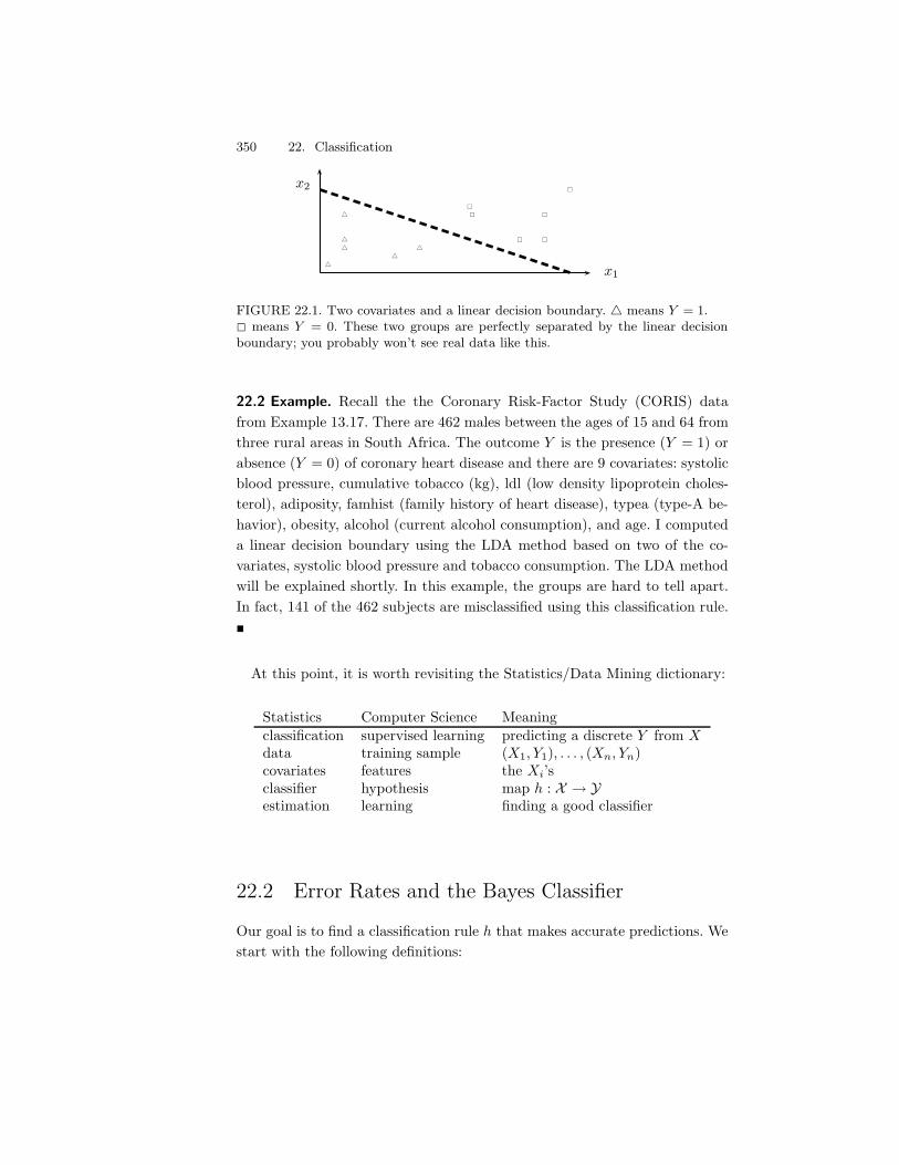
350 22. Classification
x1
x2
FIGURE 22.1. Two covariates and a linear decision boundary. ' means Y = 1.$ means Y = 0. These two groups are perfectly separated by the linear decisionboundary; you probably won’t see real data like this.
22.2 Example. Recall the the Coronary Risk-Factor Study (CORIS) datafrom Example 13.17. There are 462 males between the ages of 15 and 64 fromthree rural areas in South Africa. The outcome Y is the presence (Y = 1) orabsence (Y = 0) of coronary heart disease and there are 9 covariates: systolicblood pressure, cumulative tobacco (kg), ldl (low density lipoprotein choles-terol), adiposity, famhist (family history of heart disease), typea (type-A be-havior), obesity, alcohol (current alcohol consumption), and age. I computeda linear decision boundary using the LDA method based on two of the co-variates, systolic blood pressure and tobacco consumption. The LDA methodwill be explained shortly. In this example, the groups are hard to tell apart.In fact, 141 of the 462 subjects are misclassified using this classification rule.!
At this point, it is worth revisiting the Statistics/Data Mining dictionary:
Statistics Computer Science Meaningclassification supervised learning predicting a discrete Y from Xdata training sample (X1, Y1), . . . , (Xn, Yn)covariates features the Xi’sclassifier hypothesis map h : X ) Yestimation learning finding a good classifier
22.2 Error Rates and the Bayes Classifier
Our goal is to find a classification rule h that makes accurate predictions. Westart with the following definitions:
22.2 Error Rates and the Bayes Classifier 351
22.3 Definition. The true error rate1of a classifier h is
L(h) = P({h(X) (= Y }) (22.1)
and the empirical error rate or training error rate is
1Ln(h) =1n
n*
i=1
I(h(Xi) (= Yi). (22.2)
First we consider the special case where Y = {0, 1}. Let
r(x) = E(Y |X = x) = P(Y = 1|X = x)
denote the regression function. From Bayes’ theorem we have that
r(x) = P(Y = 1|X = x)
=f(x|Y = 1)P(Y = 1)
f(x|Y = 1)P(Y = 1) + f(x|Y = 0)P(Y = 0)
=&f1(x)
&f1(x) + (1" &)f0(x)(22.3)
where
f0(x) = f(x|Y = 0)
f1(x) = f(x|Y = 1)
& = P(Y = 1).
22.4 Definition. The Bayes classification rule h* is
h*(x) ='
1 if r(x) > 12
0 otherwise. (22.4)
The set D(h) = {x : P(Y = 1|X = x) = P(Y = 0|X = x)} is called thedecision boundary.
Warning! The Bayes rule has nothing to do with Bayesian inference. Wecould estimate the Bayes rule using either frequentist or Bayesian methods.
The Bayes rule may be written in several equivalent forms:
1One can use other loss functions. For simplicity we will use the error rate as our loss function.
352 22. Classification
h*(x) ='
1 if P(Y = 1|X = x) > P(Y = 0|X = x)0 otherwise (22.5)
andh*(x) =
'1 if &f1(x) > (1" &)f0(x)0 otherwise. (22.6)
22.5 Theorem. The Bayes rule is optimal, that is, if h is any other classifi-cation rule then L(h*) , L(h).
The Bayes rule depends on unknown quantities so we need to use the datato find some approximation to the Bayes rule. At the risk of oversimplifying,there are three main approaches:
1. Empirical Risk Minimization. Choose a set of classifiers H and find 1h $ Hthat minimizes some estimate of L(h).
2. Regression. Find an estimate 1r of the regression function r and define
1h(x) ='
1 if 1r(x) > 12
0 otherwise.
3. Density Estimation. Estimate f0 from the Xi’s for which Yi = 0, estimatef1 from the Xi’s for which Yi = 1 and let 1& = n$1
0ni=1 Yi. Define
1r(x) = 1P(Y = 1|X = x) =1& 1f1(x)
1& 1f1(x) + (1" 1&) 1f0(x)
and1h(x) =
'1 if 1r(x) > 1
20 otherwise.
Now let us generalize to the case where Y takes on more than two valuesas follows.
22.6 Theorem. Suppose that Y $ Y = {1, . . . , K}. The optimal rule is
h(x) = argmaxk P(Y = k|X = x) (22.7)
= argmaxk&k fk(x) (22.8)
whereP(Y = k|X = x) =
fk(x)&k0r fr(x)&r
, (22.9)
&r = P (Y = r), fr(x) = f(x|Y = r) and argmaxk means “the value of k
that maximizes that expression.”
22.3 Gaussian and Linear Classifiers 353
22.3 Gaussian and Linear Classifiers
Perhaps the simplest approach to classification is to use the density estima-tion strategy and assume a parametric model for the densities. Suppose thatY = {0, 1} and that f0(x) = f(x|Y = 0) and f1(x) = f(x|Y = 1) are bothmultivariate Gaussians:
fk(x) =1
(2&)d/2|'k|1/2exp'"1
2(x " µk)T'$1
k (x" µk)2
, k = 0, 1.
Thus, X |Y = 0 ! N(µ0,'0) and X |Y = 1 ! N(µ1,'1).
22.7 Theorem. If X |Y = 0 ! N(µ0,'0) and X |Y = 1 ! N(µ1,'1), then theBayes rule is
h*(x) =
:1 if r2
1 < r20 + 2 log
+-1-0
,+ log
+|#0||#1|
,
0 otherwise(22.10)
wherer2i = (x" µi)T'$1
i (x" µi), i = 1, 2 (22.11)
is the Manalahobis distance. An equivalent way of expressing the Bayes’rule is
h*(x) = argmaxk$k(x)
where
$k(x) = "12
log |'k|"12(x" µk)T'$1
k (x " µk) + log &k (22.12)
and |A| denotes the determinant of a matrix A.
The decision boundary of the above classifier is quadratic so this procedureis called quadratic discriminant analysis (QDA). In practice, we usesample estimates of &, µ1, µ2,'0,'1 in place of the true value, namely:
1&0 =1n
n*
i=1
(1" Yi), 1&1 =1n
n*
i=1
Yi
1µ0 =1n0
*
i: Yi=0
Xi, 1µ1 =1n1
*
i: Yi=1
Xi
S0 =1n0
*
i: Yi=0
(Xi " 1µ0)(Xi " 1µ0)T , S1 =1n1
*
i: Yi=1
(Xi " 1µ1)(Xi " 1µ1)T
where n0 =0
i(1" Yi) and n1 =0
i Yi.
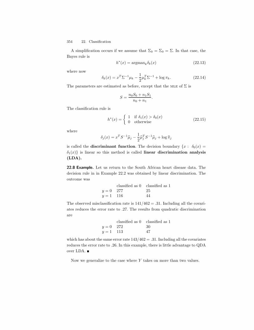
354 22. Classification
A simplification occurs if we assume that '0 = '0 = '. In that case, theBayes rule is
h*(x) = argmaxk$k(x) (22.13)
where now$k(x) = xT'$1µk "
12µT
k '$1 + log &k. (22.14)
The parameters are estimated as before, except that the mle of ' is
S =n0S0 + n1S1
n0 + n1.
The classification rule is
h*(x) ='
1 if $1(x) > $0(x)0 otherwise (22.15)
where$j(x) = xT S$11µj "
121µT
j S$11µj + log 1&j
is called the discriminant function. The decision boundary {x : $0(x) =$1(x)} is linear so this method is called linear discrimination analysis(LDA).
22.8 Example. Let us return to the South African heart disease data. Thedecision rule in in Example 22.2 was obtained by linear discrimination. Theoutcome was
classified as 0 classified as 1y = 0 277 25y = 1 116 44
The observed misclassification rate is 141/462 = .31. Including all the covari-ates reduces the error rate to .27. The results from quadratic discriminationare
classified as 0 classified as 1y = 0 272 30y = 1 113 47
which has about the same error rate 143/462 = .31. Including all the covariatesreduces the error rate to .26. In this example, there is little advantage to QDAover LDA. !
Now we generalize to the case where Y takes on more than two values.
22.3 Gaussian and Linear Classifiers 355
22.9 Theorem. Suppose that Y $ {1, . . . , K}. If fk(x) = f(x|Y = k) isGaussian, the Bayes rule is
h(x) = argmaxk$k(x)
where
$k(x) = "12
log |'k|"12(x" µk)T'$1
k (x" µk) + log &k. (22.16)
If the variances of the Gaussians are equal, then
$k(x) = xT'$1µk "12µT
k '$1 + log &k. (22.17)
We estimate $k(x) by by inserting estimates of µk, 'k and &k. There isanother version of linear discriminant analysis due to Fisher. The idea isto first reduce the dimension of covariates to one dimension by projectingthe data onto a line. Algebraically, this means replacing the covariate X =(X1, . . . , Xd) with a linear combination U = wT X =
0dj=1 wjXj . The goal is
to choose the vector w = (w1, . . . , wd) that “best separates the data.” Thenwe perform classification with the one-dimensional covariate Z instead of X .
We need define what we mean by separation of the groups. We would likethe two groups to have means that are far apart relative to their spread. Letµj denote the mean of X for Yj and let ' be the variance matrix of X . ThenE(U |Y = j) = E(wT X |Y = j) = wT µj and V(U) = wT'w. 2 Define theseparation by
J(w) =(E(U |Y = 0)" E(U |Y = 1))2
wT'w
=(wT µ0 " wT µ1)2
wT'w
=wT (µ0 " µ1)(µ0 " µ1)T w
wT'w.
We estimate J as follows. Let nj =0n
i=1 I(Yi = j) be the number of obser-vations in group j, let Xj be the sample mean vector of the X ’s for group j,and let Sj be the sample covariance matrix in group j. Define
1J(w) =wT SBw
wT SW w(22.18)
2The quantity J arises in physics, where it is called the Rayleigh coe"cient.
356 22. Classification
where
SB = (X0 "X1)(X0 "X1)T
SW =(n0 " 1)S0 + (n1 " 1)S1
(n0 " 1) + (n1 " 1).
22.10 Theorem. The vector
w = S$1W (X0 "X1) (22.19)
is a minimizer of 1J(w). We call
U = wT X = (X0 "X1)T S$1W X (22.20)
the Fisher linear discriminant function. The midpoint m between X0 andX1 is
m =12(X0 + X1) =
12(X0 "X1)T S$1
B (X0 + X1) (22.21)
Fisher’s classification rule is
h(x) ='
0 if wT X * m1 if wT X < m.
Fisher’s rule is the same as the Bayes linear classifier in equation (22.14)when 1& = 1/2.
22.4 Linear Regression and Logistic Regression
A more direct approach to classification is to estimate the regression functionr(x) = E(Y |X = x) without bothering to estimate the densities fk. For therest of this section, we will only consider the case where Y = {0, 1}. Thus,r(x) = P(Y = 1|X = x) and once we have an estimate 1r, we will use theclassification rule
1h(x) ='
1 if 1r(x) > 12
0 otherwise. (22.22)
The simplest regression model is the linear regression model
Y = r(x) + - = (0 +d*
j=1
(jXj + - (22.23)
where E(-) = 0. This model can’t be correct since it does not force Y = 0 or1. Nonetheless, it can sometimes lead to a decent classifier.
22.4 Linear Regression and Logistic Regression 357
Recall that the least squares estimate of ( = ((0,(1, . . . ,(d)T minimizesthe residual sums of squares
rss(() =n*
i=1
-Yi " (0 "
d*
j=1
Xij(j
.2
.
Let X denote the N - (d + 1) matrix of the form
X =
N
OOOP
1 X11 . . . X1d
1 X21 . . . X2d...
......
...1 Xn1 . . . Xnd
Q
RRRS.
Also let Y = (Y1, . . . , Yn)T . Then,
RSS(() = (Y "X()T (Y "X()
and the model can be written as
Y = X( + -
where - = (-1, . . . , -n)T . From Theorem 13.13,
1( = (XT X)$1XT Y.
The predicted values are1Y = X1(.
Now we use (22.22) to classify, where 1r(x) = 1(0 +0
j1(jxj .
An alternative is to use logistic regression which was also discussed in Chap-ter 13. The model is
r(x) = P(Y = 1|X = x) =e"0+
0j "jxj
1 + e"0+0
j "jxj(22.24)
and the mle 1( is obtained numerically.
22.11 Example. Let us return to the heart disease data. The mle is given inExample 13.17. The error rate, using this model for classification, is .27. Theerror rate from a linear regression is .26.
We can get a better classifier by fitting a richer model. For example, wecould fit
logit P(Y = 1|X = x) = (0 +*
j
(jxj +*
j,k
(jkxjxk. (22.25)
358 22. Classification
More generally, we could add terms of up to order r for some integer r. Largevalues of r give a more complicated model which should fit the data better.But there is a bias–variance tradeo! which we’ll discuss later.
22.12 Example. If we use model (22.25) for the heart disease data with r = 2,the error rate is reduced to .22. !
22.5 Relationship Between Logistic Regression andLDA
LDA and logistic regression are almost the same thing. If we assume that eachgroup is Gaussian with the same covariance matrix, then we saw earlier that
log-
P(Y = 1|X = x)P(Y = 0|X = x)
.= log
-&0
&1
." 1
2(µ0 + µ1)T'$1(µ1 " µ0)
+ xT'$1(µ1 " µ0)
0 )0 + )T x.
On the other hand, the logistic model is, by assumption,
log-
P(Y = 1|X = x)P(Y = 0|X = x)
.= (0 + (T x.
These are the same model since they both lead to classification rules that arelinear in x. The di!erence is in how we estimate the parameters.
The joint density of a single observation is f(x, y) = f(x|y)f(y) = f(y|x)f(x).In LDA we estimated the whole joint distribution by maximizing the likeli-hood /
i
f(xi, yi) =/
i
f(xi|yi)
a b_ `Gaussian
/
i
f(yi)
a b_ `Bernoulli
. (22.26)
In logistic regression we maximized the conditional likelihoodD
i f(yi|xi) butwe ignored the second term f(xi):
/
i
f(xi, yi) =/
i
f(yi|xi)
a b_ `logistic
/
i
f(xi)
a b_ `ignored
. (22.27)
Since classification only requires knowing f(y|x), we don’t really need to es-timate the whole joint distribution. Logistic regression leaves the marginal
22.6 Density Estimation and Naive Bayes 359
distribution f(x) unspecified so it is more nonparametric than LDA. This isan advantage of the logistic regression approach over LDA.
To summarize: LDA and logistic regression both lead to a linear classi-fication rule. In LDA we estimate the entire joint distribution f(x, y) =f(x|y)f(y). In logistic regression we only estimate f(y|x) and we don’t botherestimating f(x).
22.6 Density Estimation and Naive Bayes
The Bayes rule is h(x) = argmaxk &k fk(x). If we can estimate &k and fk
then we can estimate the Bayes classification rule. Estimating &k is easy butwhat about fk? We did this previously by assuming fk was Gaussian. An-other strategy is to estimate fk with some nonparametric density estimator1fk such as a kernel estimator. But if x = (x1, . . . , xd) is high-dimensional,nonparametric density estimation is not very reliable. This problem is amelio-rated if we assume that X1, . . . , Xd are independent, for then, fk(x1, . . . , xd) =Dd
j=1 fkj(xj). This reduces the problem to d one-dimensional density estima-tion problems, within each of the k groups. The resulting classifier is calledthe naive Bayes classifier. The assumption that the components of X areindependent is usually wrong yet the resulting classifier might still be accu-rate. Here is a summary of the steps in the naive Bayes classifier:
The Naive Bayes Classifier
1. For each group k, compute an estimate 1fkj of the density fkj for Xj ,using the data for which Yi = k.
2. Let
1fk(x) = 1fk(x1, . . . , xd) =d/
j=1
1fkj(xj).
3. Let
1&k =1n
n*
i=1
I(Yi = k)
where I(Yi = k) = 1 if Yi = k and I(Yi = k) = 0 if Yi (= k.
4. Leth(x) = argmaxk 1&k
1fk(x).
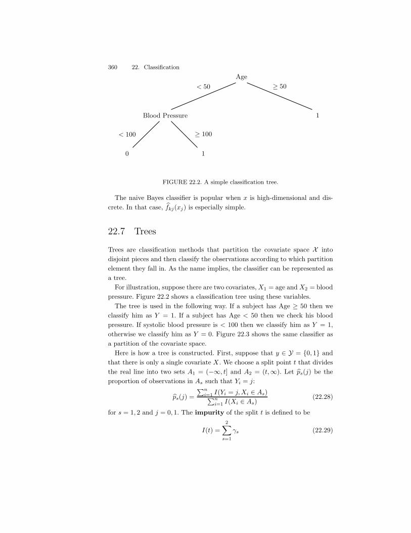
360 22. Classification
0 1
Blood Pressure 1
Age
< 100 * 100
< 50 * 50
FIGURE 22.2. A simple classification tree.
The naive Bayes classifier is popular when x is high-dimensional and dis-crete. In that case, 1fkj(xj) is especially simple.
22.7 Trees
Trees are classification methods that partition the covariate space X intodisjoint pieces and then classify the observations according to which partitionelement they fall in. As the name implies, the classifier can be represented asa tree.
For illustration, suppose there are two covariates, X1 = age and X2 = bloodpressure. Figure 22.2 shows a classification tree using these variables.
The tree is used in the following way. If a subject has Age * 50 then weclassify him as Y = 1. If a subject has Age < 50 then we check his bloodpressure. If systolic blood pressure is < 100 then we classify him as Y = 1,otherwise we classify him as Y = 0. Figure 22.3 shows the same classifier asa partition of the covariate space.
Here is how a tree is constructed. First, suppose that y $ Y = {0, 1} andthat there is only a single covariate X . We choose a split point t that dividesthe real line into two sets A1 = ("#, t] and A2 = (t,#). Let 1ps(j) be theproportion of observations in As such that Yi = j:
1ps(j) =0n
i=1 I(Yi = j, Xi $ As)0ni=1 I(Xi $ As)
(22.28)
for s = 1, 2 and j = 0, 1. The impurity of the split t is defined to be
I(t) =2*
s=1
/s (22.29)
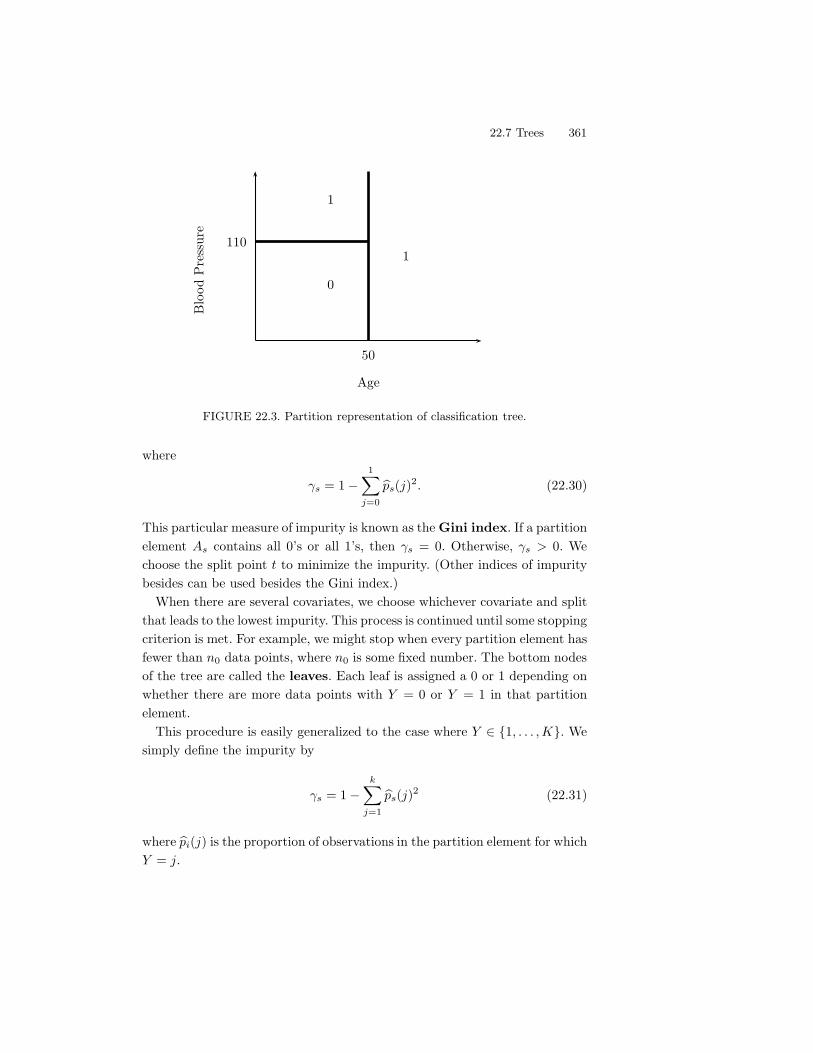
22.7 Trees 361
1
0
1
Age
Blo
odP
ress
ure
50
110
FIGURE 22.3. Partition representation of classification tree.
where
/s = 1"1*
j=0
1ps(j)2. (22.30)
This particular measure of impurity is known as the Gini index. If a partitionelement As contains all 0’s or all 1’s, then /s = 0. Otherwise, /s > 0. Wechoose the split point t to minimize the impurity. (Other indices of impuritybesides can be used besides the Gini index.)
When there are several covariates, we choose whichever covariate and splitthat leads to the lowest impurity. This process is continued until some stoppingcriterion is met. For example, we might stop when every partition element hasfewer than n0 data points, where n0 is some fixed number. The bottom nodesof the tree are called the leaves. Each leaf is assigned a 0 or 1 depending onwhether there are more data points with Y = 0 or Y = 1 in that partitionelement.
This procedure is easily generalized to the case where Y $ {1, . . . , K}. Wesimply define the impurity by
/s = 1"k*
j=1
1ps(j)2 (22.31)
where 1pi(j) is the proportion of observations in the partition element for whichY = j.
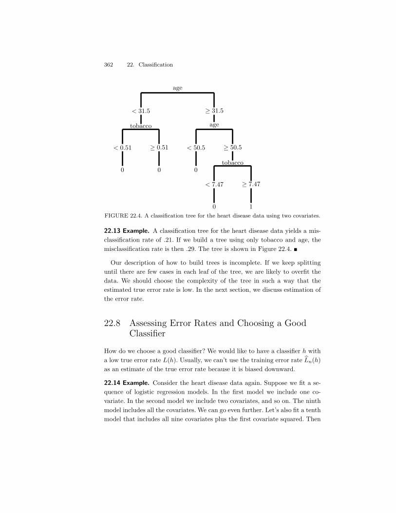
362 22. Classification
tobacco
< 0.51 * 0.51
age
< 31.5 * 31.5
age
< 50.5 * 50.5
tobacco
< 7.47 * 7.47
0 0 0
0 1FIGURE 22.4. A classification tree for the heart disease data using two covariates.
22.13 Example. A classification tree for the heart disease data yields a mis-classification rate of .21. If we build a tree using only tobacco and age, themisclassification rate is then .29. The tree is shown in Figure 22.4. !
Our description of how to build trees is incomplete. If we keep splittinguntil there are few cases in each leaf of the tree, we are likely to overfit thedata. We should choose the complexity of the tree in such a way that theestimated true error rate is low. In the next section, we discuss estimation ofthe error rate.
22.8 Assessing Error Rates and Choosing a GoodClassifier
How do we choose a good classifier? We would like to have a classifier h witha low true error rate L(h). Usually, we can’t use the training error rate 1Ln(h)as an estimate of the true error rate because it is biased downward.
22.14 Example. Consider the heart disease data again. Suppose we fit a se-quence of logistic regression models. In the first model we include one co-variate. In the second model we include two covariates, and so on. The ninthmodel includes all the covariates. We can go even further. Let’s also fit a tenthmodel that includes all nine covariates plus the first covariate squared. Then
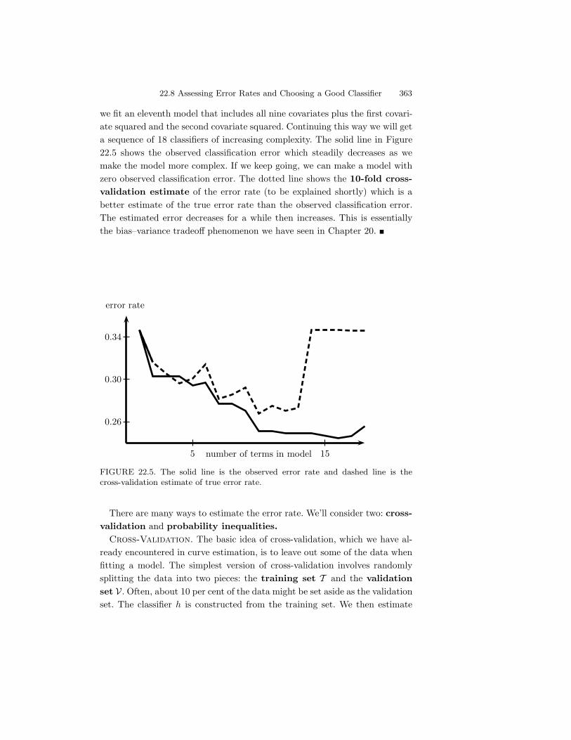
22.8 Assessing Error Rates and Choosing a Good Classifier 363
we fit an eleventh model that includes all nine covariates plus the first covari-ate squared and the second covariate squared. Continuing this way we will geta sequence of 18 classifiers of increasing complexity. The solid line in Figure22.5 shows the observed classification error which steadily decreases as wemake the model more complex. If we keep going, we can make a model withzero observed classification error. The dotted line shows the 10-fold cross-validation estimate of the error rate (to be explained shortly) which is abetter estimate of the true error rate than the observed classification error.The estimated error decreases for a while then increases. This is essentiallythe bias–variance tradeo! phenomenon we have seen in Chapter 20. !
number of terms in model
error rate
0.26
0.30
0.34
5 15
FIGURE 22.5. The solid line is the observed error rate and dashed line is thecross-validation estimate of true error rate.
There are many ways to estimate the error rate. We’ll consider two: cross-validation and probability inequalities.
Cross-Validation. The basic idea of cross-validation, which we have al-ready encountered in curve estimation, is to leave out some of the data whenfitting a model. The simplest version of cross-validation involves randomlysplitting the data into two pieces: the training set T and the validationset V . Often, about 10 per cent of the data might be set aside as the validationset. The classifier h is constructed from the training set. We then estimate
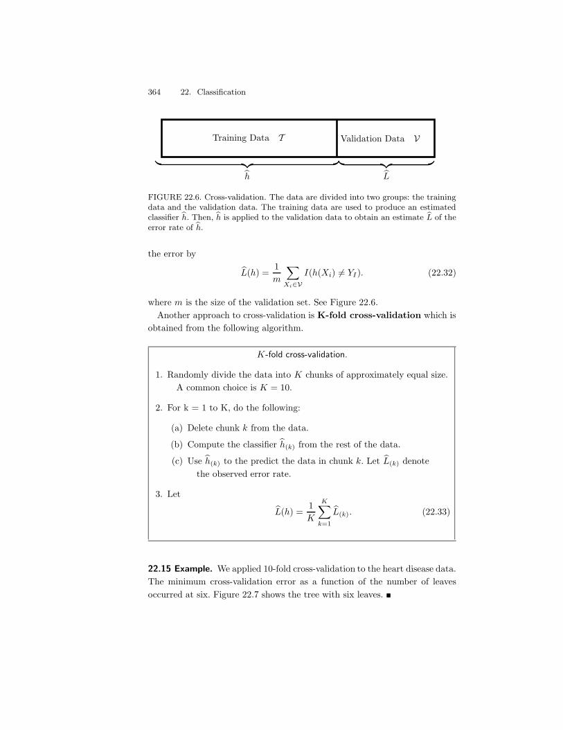
364 22. Classification
Training Data T Validation Data V
a b_ `1h
a b_ `1L
FIGURE 22.6. Cross-validation. The data are divided into two groups: the trainingdata and the validation data. The training data are used to produce an estimatedclassifier 1h. Then, 1h is applied to the validation data to obtain an estimate 1L of theerror rate of 1h.
the error by
1L(h) =1m
*
Xi#VI(h(Xi) (= YI). (22.32)
where m is the size of the validation set. See Figure 22.6.Another approach to cross-validation is K-fold cross-validation which is
obtained from the following algorithm.
K-fold cross-validation.
1. Randomly divide the data into K chunks of approximately equal size.A common choice is K = 10.
2. For k = 1 to K, do the following:
(a) Delete chunk k from the data.
(b) Compute the classifier 1h(k) from the rest of the data.
(c) Use 1h(k) to the predict the data in chunk k. Let 1L(k) denotethe observed error rate.
3. Let
1L(h) =1K
K*
k=1
1L(k). (22.33)
22.15 Example. We applied 10-fold cross-validation to the heart disease data.The minimum cross-validation error as a function of the number of leavesoccurred at six. Figure 22.7 shows the tree with six leaves. !
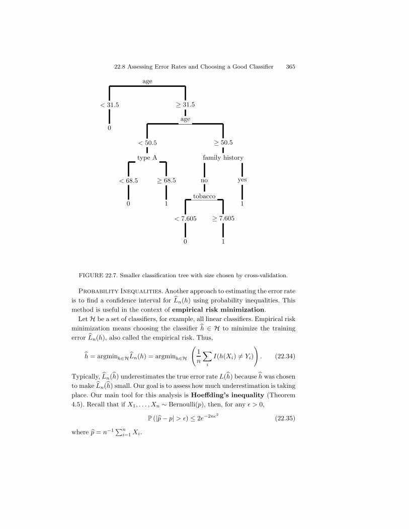
22.8 Assessing Error Rates and Choosing a Good Classifier 365
age
< 31.5 * 31.5
age
< 50.5 * 50.5
type A
< 68.5 * 68.5
family history
no yes
tobacco
< 7.605 * 7.605
0
0 1
0 1
1
FIGURE 22.7. Smaller classification tree with size chosen by cross-validation.
Probability Inequalities. Another approach to estimating the error rateis to find a confidence interval for 1Ln(h) using probability inequalities. Thismethod is useful in the context of empirical risk minimization.
Let H be a set of classifiers, for example, all linear classifiers. Empirical riskminimization means choosing the classifier 1h $ H to minimize the trainingerror 1Ln(h), also called the empirical risk. Thus,
1h = argminh#H1Ln(h) = argminh#H
(1n
*
i
I(h(Xi) (= Yi)
). (22.34)
Typically, 1Ln(1h) underestimates the true error rate L(1h) because 1h was chosento make 1Ln(1h) small. Our goal is to assess how much underestimation is takingplace. Our main tool for this analysis is Hoe"ding’s inequality (Theorem4.5). Recall that if X1, . . . , Xn ! Bernoulli(p), then, for any - > 0,
P (|1p" p| > -) , 2e$2n&2 (22.35)
where 1p = n$10n
i=1 Xi.
366 22. Classification
First, suppose that H = {h1, . . . , hm} consists of finitely many classifiers.For any fixed h, 1Ln(h) converges in almost surely to L(h) by the law of largenumbers. We will now establish a stronger result.
22.16 Theorem (Uniform Convergence). Assume H is finite and has m ele-ments. Then,
P-
maxh#H
|1Ln(h)" L(h)| > -
., 2me$2n&2.
Proof. We will use Hoe!ding’s inequality and we will also use the factthat if A1, . . . , Am is a set of events then P(
&mi=1 Ai) ,
0mi=1 P(Ai). Now,
P-
maxh#H
|1Ln(h)" L(h)| > -
.= P
(#
h#H|1Ln(h)" L(h)| > -
)
,*
H#HP+|1Ln(h)" L(h)| > -
,
,*
H#H2e$2n&2 = 2me$2n&2 . !
22.17 Theorem. Let
- =
T2n
log-
2m
)
..
Then 1Ln(1h) ± - is a 1" ) confidence interval for L(1h).
Proof. This follows from the fact that
P(|1Ln(1h)" L(1h)| > -) , P-
maxh#H
|1Ln(1h)" L(1h)| > -
.
, 2me$2n&2 = ). !
When H is large the confidence interval for L(1h) is large. The more functionsthere are in H the more likely it is we have “overfit” which we compensatefor by having a larger confidence interval.
In practice we usually use sets H that are infinite, such as the set of linearclassifiers. To extend our analysis to these cases we want to be able to saysomething like
P-
suph#H
|1Ln(h)" L(h)| > -
., something not too big.
One way to develop such a generalization is by way of the Vapnik-Chervonenkisor VC dimension.
22.8 Assessing Error Rates and Choosing a Good Classifier 367
Let A be a class of sets. Give a finite set F = {x1, . . . , xn} let
NA(F ) = #'
F$
A : A $ A2
(22.36)
be the number of subsets of F “picked out” by A. Here #(B) denotes thenumber of elements of a set B. The shatter coe!cient is defined by
s(A, n) = maxF#Fn
NA(F ) (22.37)
where Fn consists of all finite sets of size n. Now let X1, . . . , Xn ! P and let
Pn(A) =1n
*
i
I(Xi $ A)
denote the empirical probability measure. The following remarkable the-orem bounds the distance between P and Pn.
22.18 Theorem (Vapnik and Chervonenkis (1971)). For any P, n and - > 0,
P'
supA#A
|Pn(A) " P(A)| > -
2, 8s(A, n)e$n&2/32. (22.38)
The proof, though very elegant, is long and we omit it. If H is a set ofclassifiers, define A to be the class of sets of the form {x : h(x) = 1}. Wethen define s(H, n) = s(A, n).
22.19 Theorem.
P'
suph#H
|1Ln(h)" L(h)| > -
2, 8s(H, n)e$n&2/32.
A 1" ) confidence interval for L(1h) is 1Ln(1h) ± -n where
-2n =32n
log-
8s(H, n))
..
These theorems are only useful if the shatter coe#cients do not grow tooquickly with n. This is where VC dimension enters.
22.20 Definition. The VC (Vapnik-Chervonenkis) dimension of a class ofsets A is defined as follows. If s(A, n) = 2n for all n, set V C(A) =#.Otherwise, define V C(A) to be the largest k for which s(A, n) = 2k.
Thus, the VC-dimension is the size of the largest finite set F that can beshattered by A meaning that A picks out each subset of F . If H is a set ofclassifiers we define V C(H) = V C(A) where A is the class of sets of the form{x : h(x) = 1} as h varies in H. The following theorem shows that if A hasfinite VC-dimension, then the shatter coe#cients grow as a polynomial in n.
368 22. Classification
22.21 Theorem. If A has finite VC-dimension v, then
s(A, n) , nv + 1.
22.22 Example. Let A = {("#, a]; a $ R}. The A shatters every 1-pointset {x} but it shatters no set of the form {x, y}. Therefore, V C(A) = 1. !
22.23 Example. Let A be the set of closed intervals on the real line. ThenA shatters S = {x, y} but it cannot shatter sets with 3 points. ConsiderS = {x, y, z} where x < y < z. One cannot find an interval A such thatA%
S = {x, z}. So, V C(A) = 2. !
22.24 Example. Let A be all linear half-spaces on the plane. Any 3-pointset (not all on a line) can be shattered. No 4 point set can be shattered.Consider, for example, 4 points forming a diamond. Let T be the left andrightmost points. This can’t be picked out. Other configurations can also beseen to be unshatterable. So V C(A) = 3. In general, halfspaces in Rd haveVC dimension d + 1. !
22.25 Example. Let A be all rectangles on the plane with sides parallel tothe axes. Any 4 point set can be shattered. Let S be a 5 point set. There isone point that is not leftmost, rightmost, uppermost, or lowermost. Let T beall points in S except this point. Then T can’t be picked out. So V C(A) = 4.!
22.26 Theorem. Let x have dimension d and let H be th set of linear classi-fiers. The VC-dimension of H is d + 1. Hence, a 1") confidence interval forthe true error rate is 1L(1h) ± - where
-2n =32n
log-
8(nd+1 + 1))
..
22.9 Support Vector Machines
In this section we consider a class of linear classifiers called support vectormachines. Throughout this section, we assume that Y is binary. It will beconvenient to label the outcomes as "1 and +1 instead of 0 and 1. A linearclassifier can then be written as
h(x) = sign-
H(x).
22.9 Support Vector Machines 369
where x = (x1, . . . , xd),
H(x) = a0 +d*
i=1
aixi
and
sign(z) =
46
7
"1 if z < 00 if z = 01 if z > 0.
First, suppose that the data are linearly separable, that is, there existsa hyperplane that perfectly separates the two classes.
22.27 Lemma. The data can be separated by some hyperplane if and only ifthere exists a hyperplane H(x) = a0 +
0di=1 aixi such that
YiH(xi) * 1, i = 1, . . . , n. (22.39)
Proof. Suppose the data can be separated by a hyperplane W (x) = b0 +0di=1 bixi. It follows that there exists some constant c such that Yi = 1 implies
W (Xi) * c and Yi = "1 implies W (Xi) , "c. Therefore, YiW (Xi) * c forall i. Let H(x) = a0 +
0di=1 aixi where aj = bj/c. Then YiH(Xi) * 1 for all
i. The reverse direction is straightforward. !
In the separable case, there will be many separating hyperplanes. Howshould we choose one? Intuitively, it seems reasonable to choose the hyper-plane “furthest” from the data in the sense that it separates the +1s and -1sand maximizes the distance to the closest point. This hyperplane is called themaximum margin hyperplane. The margin is the distance to from thehyperplane to the nearest point. Points on the boundary of the margin arecalled support vectors. See Figure 22.8.
22.28 Theorem. The hyperplane 1H(x) = 1a0 +0d
i=1 1aixi that separates thedata and maximizes the margin is given by minimizing (1/2)
0dj=1 a2
j subjectto (22.39).
It turns out that this problem can be recast as a quadratic programmingproblem. Let 6Xi, Xk7 = XT
i Xk denote the inner product of Xi and Xk.
22.29 Theorem. Let 1H(x) = 1a0 +0d
i=1 1aixi denote the optimal (largest mar-gin) hyperplane. Then, for j = 1, . . . , d,
1aj =n*
i=1
1)iYiXj(i)
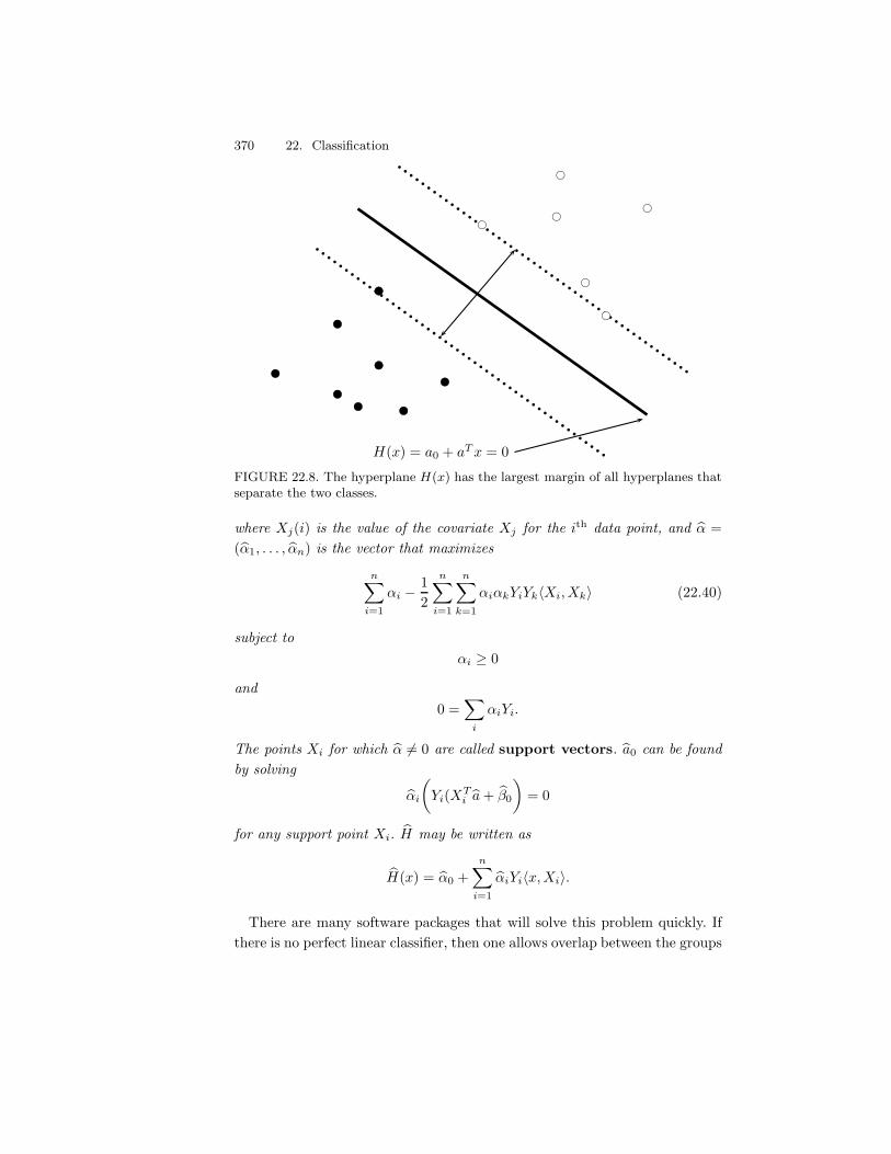
370 22. Classification
H(x) = a0 + aT x = 0
FIGURE 22.8. The hyperplane H(x) has the largest margin of all hyperplanes thatseparate the two classes.
where Xj(i) is the value of the covariate Xj for the ith data point, and 1) =(1)1, . . . , 1)n) is the vector that maximizes
n*
i=1
)i "12
n*
i=1
n*
k=1
)i)kYiYk6Xi, Xk7 (22.40)
subject to)i * 0
and0 =
*
i
)iYi.
The points Xi for which 1) (= 0 are called support vectors. 1a0 can be foundby solving
1)i
-Yi(XT
i 1a + 1(0
.= 0
for any support point Xi. 1H may be written as
1H(x) = 1)0 +n*
i=1
1)iYi6x, Xi7.
There are many software packages that will solve this problem quickly. Ifthere is no perfect linear classifier, then one allows overlap between the groups
22.10 Kernelization 371
by replacing the condition (22.39) with
YiH(xi) * 1" .i, .i * 0, i = 1, . . . , n. (22.41)
The variables .1, . . . , .n are called slack variables.We now maximize (22.40) subject to
0 , .i , c, i = 1, . . . , n
andn*
i=1
)iYi = 0.
The constant c is a tuning parameter that controls the amount of overlap.
22.10 Kernelization
There is a trick called kernelization for improving a computationally simpleclassifier h. The idea is to map the covariate X — which takes values in X —into a higher dimensional space Z and apply the classifier in the bigger spaceZ. This can yield a more flexible classifier while retaining computationallysimplicity.
The standard example of this idea is illustrated in Figure 22.9. The covariatex = (x1, x2). The Yis can be separated into two groups using an ellipse. Definea mapping ' by
z = (z1, z2, z3) = '(x) = (x21,/
2x1x2, x22).
Thus, ' maps X = R2 into Z = R3. In the higher-dimensional space Z, theYi’s are separable by a linear decision boundary. In other words,
a linear classifier in a higher-dimensional space corresponds to a non-
linear classifier in the original space.
The point is that to get a richer set of classifiers we do not need to give up theconvenience of linear classifiers. We simply map the covariates to a higher-dimensional space. This is akin to making linear regression more flexible byusing polynomials.
There is a potential drawback. If we significantly expand the dimensionof the problem, we might increase the computational burden. For example,if x has dimension d = 256 and we wanted to use all fourth-order terms,then z = '(x) has dimension 183,181,376. We are spared this computational
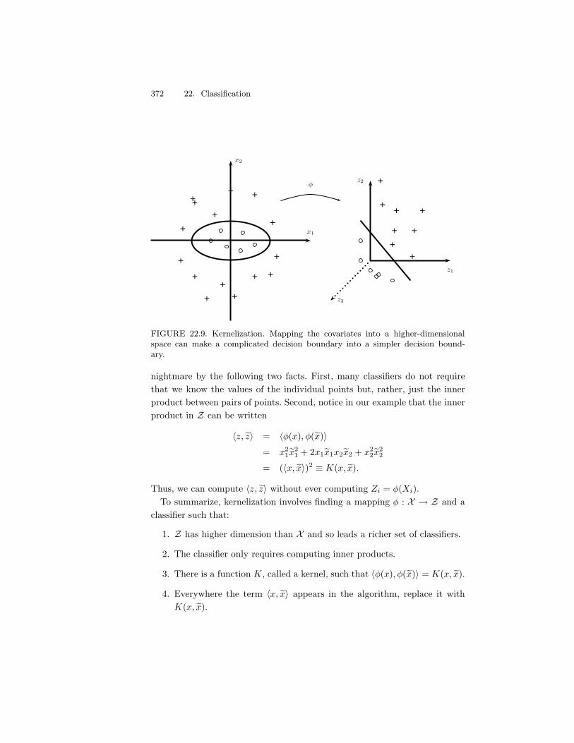
372 22. Classification
x1
x2
+
+
+
+++
+ +
+
+
+++
+ +
z1
z2
z3
+
+
++
+
+
+
+
'
FIGURE 22.9. Kernelization. Mapping the covariates into a higher-dimensionalspace can make a complicated decision boundary into a simpler decision bound-ary.
nightmare by the following two facts. First, many classifiers do not requirethat we know the values of the individual points but, rather, just the innerproduct between pairs of points. Second, notice in our example that the innerproduct in Z can be written
6z, cz7 = 6'(x),'(cx)7= x2
1cx21 + 2x1cx1x2cx2 + x2
2cx22
= (6x, cx7)2 0 K(x, cx).
Thus, we can compute 6z, cz7 without ever computing Zi = '(Xi).To summarize, kernelization involves finding a mapping ' : X ) Z and a
classifier such that:
1. Z has higher dimension than X and so leads a richer set of classifiers.
2. The classifier only requires computing inner products.
3. There is a function K, called a kernel, such that 6'(x),'(cx)7 = K(x, cx).
4. Everywhere the term 6x, cx7 appears in the algorithm, replace it withK(x, cx).
22.10 Kernelization 373
In fact, we never need to construct the mapping ' at all. We only needto specify a kernel K(x, cx) that corresponds to 6'(x),'(cx)7 for some '. Thisraises an interesting question: given a function of two variables K(x, y), doesthere exist a function '(x) such that K(x, y) = 6'(x),'(y)7? The answer isprovided by Mercer’s theorem which says, roughly, that if K is positivedefinite — meaning that
9 9K(x, y)f(x)f(y)dxdy * 0
for square integrable functions f — then such a ' exists. Examples of com-monly used kernels are:
polynomial K(x, cx) =-6x, cx7+ a
.r
sigmoid K(x, cx) = tanh(a6x, cx7+ b)
Gaussian K(x, cx) = exp-"||x" cx||2/(2#2)
.
Let us now see how we can use this trick in LDA and in support vectormachines.
Recall that the Fisher linear discriminant method replaces X with U =wT X where w is chosen to maximize the Rayleigh coe#cient
J(w) =wT SBw
wT SW w,
SB = (X0 "X1)(X0 "X1)T
andSW =
-(n0 " 1)S0
(n0 " 1) + (n1 " 1)
.+-
(n1 " 1)S1
(n0 " 1) + (n1 " 1)
..
In the kernelized version, we replace Xi with Zi = '(Xi) and we find w tomaximize
J(w) =wT cSBw
wT cSW w(22.42)
wherecSB = (Z0 " Z1)(Z0 " Z1)T
and
SW =
((n0 " 1)cS0
(n0 " 1) + (n1 " 1)
)+
((n1 " 1)cS1
(n0 " 1) + (n1 " 1)
).
Here, cSj is the sample of covariance of the Zi’s for which Y = j. However, totake advantage of kernelization, we need to re-express this in terms of innerproducts and then replace the inner products with kernels.
374 22. Classification
It can be shown that the maximizing vector w is a linear combination ofthe Zi’s. Hence we can write
w =n*
i=1
)iZi.
Also,
Zj =1nj
n*
i=1
'(Xi)I(Yi = j).
Therefore,
wT Zj =- n*
i=1
)iZi
.T- 1nj
n*
i=1
'(Xi)I(Yi = j).
=1nj
n*
i=1
n*
s=1
)iI(Ys = j)ZTi '(Xs)
=1nj
n*
i=1
)i
n*
s=1
I(Ys = j)'(Xi)T'(Xs)
=1nj
n*
i=1
)i
n*
s=1
I(Ys = j)K(Xi, Xs)
= )T Mj
where Mj is a vector whose ith component is
Mj(i) =1nj
n*
s=1
K(Xi, Xs)I(Yi = j).
It follows thatwT cSBw = )T M)
where M = (M0 "M1)(M0 "M1)T . By similar calculations, we can write
wT cSW w = )T N)
whereN = K0
-I " 1
n01.
KT0 + K1
-I " 1
n11.
KT1 ,
I is the identity matrix, 1 is a matrix of all one’s, and Kj is the n - nj
matrix with entries (Kj)rs = K(xr, xs) with xs varying over the observationsin group j. Hence, we now find ) to maximize
J()) =)T M)
)T N).
22.11 Other Classifiers 375
All the quantities are expressed in terms of the kernel. Formally, the solutionis ) = N$1(M0 "M1). However, N might be non-invertible. In this case onereplaces N by N + bI, for some constant b. Finally, the projection onto thenew subspace can be written as
U = wT'(x) =n*
i=1
)iK(xi, x).
The support vector machine can similarly be kernelized. We simply replace6Xi, Xj7 with K(Xi, Xj). For example, instead of maximizing (22.40), we nowmaximize
n*
i=1
)i "12
n*
i=1
n*
k=1
)i)kYiYkK(Xi, Xj). (22.43)
The hyperplane can be written as 1H(x) = 1a0 +0n
i=1 1)iYiK(X, Xi).
22.11 Other Classifiers
There are many other classifiers and space precludes a full discussion of all ofthem. Let us briefly mention a few.
The k-nearest-neighbors classifier is very simple. Given a point x, findthe k data points closest to x. Classify x using the majority vote of these k
neighbors. Ties can be broken randomly. The parameter k can be chosen bycross-validation.
Bagging is a method for reducing the variability of a classifier. It is mosthelpful for highly nonlinear classifiers such as trees. We draw B bootstrapsamples from the data. The bth bootstrap sample yields a classifier hb. Thefinal classifier is
1h(x) ='
1 if 1B
0Bb=1 hb(x) * 1
20 otherwise.
Boosting is a method for starting with a simple classifier and graduallyimproving it by refitting the data giving higher weight to misclassified samples.Suppose that H is a collection of classifiers, for example, trees with onlyone split. Assume that Yi $ {"1, 1} and that each h is such that h(x) ${"1, 1}. We usually give equal weight to all data points in the methods wehave discussed. But one can incorporate unequal weights quite easily in mostalgorithms. For example, in constructing a tree, we could replace the impuritymeasure with a weighted impurity measure. The original version of boosting,called AdaBoost, is as follows.
376 22. Classification
1. Set the weights wi = 1/n, i = 1, . . . , n.
2. For j = 1, . . . , J , do the following steps:
(a) Constructing a classifier hj from the data using the weights w1, . . . , wn.
(b) Compute the weighted error estimate:
1Lj =0n
i=1 wiI(Yi (= hj(Xi))0ni=1 wi
.
(c) Let )j = log((1" 1Lj)/1Lj).
(d) Update the weights:
wi 4" wie#jI(Yi .=hj(Xi))
3. The final classifier is
1h(x) = sign- J*
j=1
)jhj(x).
.
There is now an enormous literature trying to explain and improve onboosting. Whereas bagging is a variance reduction technique, boosting canbe thought of as a bias reduction technique. We starting with a simple —and hence highly-biased — classifier, and we gradually reduce the bias. Thedisadvantage of boosting is that the final classifier is quite complicated.
Neural Networks are regression models of the form 3
Y = (0 +p*
j=1
(j#()0 + )T X)
where # is a smooth function, often taken to be #(v) = ev/(1 + ev). Thisis really nothing more than a nonlinear regression model. Neural nets werefashionable for some time but they pose great computational di#culties. Inparticular, one often encounters multiple minima when trying to find the leastsquares estimates of the parameters. Also, the number of terms p is essentiallya smoothing parameter and there is the usual problem of trying to choose p
to find a good balance between bias and variance.
3This is the simplest version of a neural net. There are more complex versions of the model.
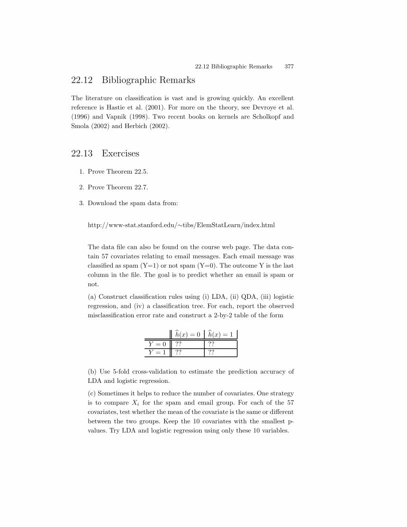
22.12 Bibliographic Remarks 377
22.12 Bibliographic Remarks
The literature on classification is vast and is growing quickly. An excellentreference is Hastie et al. (2001). For more on the theory, see Devroye et al.(1996) and Vapnik (1998). Two recent books on kernels are Scholkopf andSmola (2002) and Herbich (2002).
22.13 Exercises
1. Prove Theorem 22.5.
2. Prove Theorem 22.7.
3. Download the spam data from:
http://www-stat.stanford.edu/!tibs/ElemStatLearn/index.html
The data file can also be found on the course web page. The data con-tain 57 covariates relating to email messages. Each email message wasclassified as spam (Y=1) or not spam (Y=0). The outcome Y is the lastcolumn in the file. The goal is to predict whether an email is spam ornot.
(a) Construct classification rules using (i) LDA, (ii) QDA, (iii) logisticregression, and (iv) a classification tree. For each, report the observedmisclassification error rate and construct a 2-by-2 table of the form
1h(x) = 0 1h(x) = 1Y = 0 ?? ??Y = 1 ?? ??
(b) Use 5-fold cross-validation to estimate the prediction accuracy ofLDA and logistic regression.
(c) Sometimes it helps to reduce the number of covariates. One strategyis to compare Xi for the spam and email group. For each of the 57covariates, test whether the mean of the covariate is the same or di!erentbetween the two groups. Keep the 10 covariates with the smallest p-values. Try LDA and logistic regression using only these 10 variables.
378 22. Classification
4. Let A be the set of two-dimensional spheres. That is, A $ A if A ={(x, y) : (x"a)2+(y"b)2 , c2} for some a, b, c. Find the VC-dimensionof A.
5. Classify the spam data using support vector machines. Free software forthe support vector machine is at http://svmlight.joachims.org/
6. Use VC theory to get a confidence interval on the true error rate of theLDA classifier for the iris data (from the book web site).
7. Suppose that Xi $ R and that Yi = 1 whenever |Xi| , 1 and Yi = 0whenever |Xi| > 1. Show that no linear classifier can perfectly classifythese data. Show that the kernelized data Zi = (Xi, X2
i ) can be linearlyseparated.
8. Repeat question 5 using the kernel K(x, cx) = (1 + xT cx)p. Choose p bycross-validation.
9. Apply the k nearest neighbors classifier to the “iris data.” Choose k bycross-validation.
10. (Curse of Dimensionality.) Suppose that X has a uniform distributionon the d-dimensional cube ["1/2, 1/2]d. Let R be the distance from theorigin to the closest neighbor. Show that the median of R is
E
G
+1";
12
<1/n,
vd(1)
H
J
1/d
where
vd(r) = rd &d/2
&((d/2) + 1)
is the volume of a sphere of radius r. For what dimension d does themedian of R exceed the edge of the cube when n = 100, n = 1, 000,n = 10, 000? (Hastie et al. (2001), p. 22–27.)
11. Fit a tree to the data in question 3. Now apply bagging and report yourresults.
12. Fit a tree that uses only one split on one variable to the data in question3. Now apply boosting.
22.13 Exercises 379
13. Let r(x) = P(Y = 1|X = x) and let 1r(x) be an estimate of r(x). Considerthe classifier
h(x) ='
1 if 1r(x) * 1/20 otherwise.
Assume that 1r(x) . N(r(x),#2(x)) for some functions r(x) and #2(x).Show that, for fixed x,
P(Y (= h(x)) . P(Y (= h*(x))
+
CCCCC2r(x) " 1
CCCCC -
N
OOP1" %
E
FFG
sign-
r(x) " (1/2).
(r(x)" (1/2))
#(x)
H
IIJ
Q
RRS
where % is the standard Normal cdf and h* is the Bayes rule. Regard
sign-
(r(x) " (1/2))(r(x) " (1/2)).
as a type of bias term. Explain the
implications for the bias–variance tradeo! in classification (Friedman(1997)).
Hint: first show that
P(Y (= h(x)) = |2r(x) " 1|P(h(x) (= h*(x)) + P(Y (= h*(x)).

This is page 380Printer: Opaque this
This is page 381Printer: Opaque this
23Probability Redux: Stochastic Processes
23.1 Introduction
Most of this book has focused on iid sequences of random variables. Now weconsider sequences of dependent random variables. For example, daily tem-peratures will form a sequence of time-ordered random variables and clearlythe temperature on one day is not independent of the temperature on theprevious day.
A stochastic process {Xt : t $ T } is a collection of random variables.We shall sometimes write X(t) instead of Xt. The variables Xt take values insome set X called the state space. The set T is called the index set andfor our purposes can be thought of as time. The index set can be discreteT = {0, 1, 2, . . .} or continuous T = [0,#) depending on the application.
23.1 Example (iid observations). A sequence of iid random variables can bewritten as {Xt : t $ T } where T = {1, 2, 3, . . . , }. Thus, a sequence of iid
random variables is an example of a stochastic process. !
23.2 Example (The Weather). Let X = {sunny, cloudy}. A typical sequence(depending on where you live) might be
sunny, sunny, cloudy, sunny, cloudy, cloudy, · · ·
This process has a discrete state space and a discrete index set. !
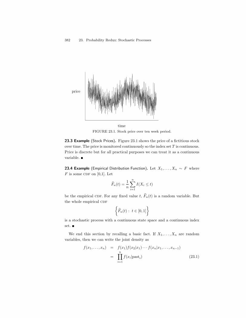
382 23. Probability Redux: Stochastic Processes
time
price
FIGURE 23.1. Stock price over ten week period.
23.3 Example (Stock Prices). Figure 23.1 shows the price of a fictitious stockover time. The price is monitored continuously so the index set T is continuous.Price is discrete but for all practical purposes we can treat it as a continuousvariable. !
23.4 Example (Empirical Distribution Function). Let X1, . . . , Xn ! F whereF is some cdf on [0,1]. Let
1Fn(t) =1n
n*
i=1
I(Xi , t)
be the empirical cdf. For any fixed value t, 1Fn(t) is a random variable. Butthe whole empirical cdf
'1Fn(t) : t $ [0, 1]
2
is a stochastic process with a continuous state space and a continuous indexset. !
We end this section by recalling a basic fact. If X1, . . . , Xn are randomvariables, then we can write the joint density as
f(x1, . . . , xn) = f(x1)f(x2|x1) · · · f(xn|x1, . . . , xn$1)
=n/
i=1
f(xi|pasti) (23.1)
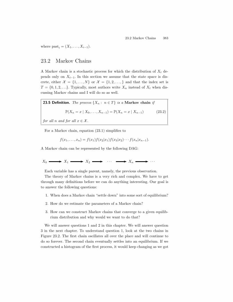
23.2 Markov Chains 383
where pasti = (X1, . . . , Xi$1).
23.2 Markov Chains
A Markov chain is a stochastic process for which the distribution of Xt de-pends only on Xt$1. In this section we assume that the state space is dis-crete, either X = {1, . . . , N} or X = {1, 2, . . . , } and that the index set isT = {0, 1, 2, . . .}. Typically, most authors write Xn instead of Xt when dis-cussing Markov chains and I will do so as well.
23.5 Definition. The process {Xn : n $ T } is a Markov chain if
P(Xn = x | X0, . . . , Xn$1) = P(Xn = x | Xn$1) (23.2)
for all n and for all x $ X .
For a Markov chain, equation (23.1) simplifies to
f(x1, . . . , xn) = f(x1)f(x2|x1)f(x3|x2) · · · f(xn|xn$1).
A Markov chain can be represented by the following DAG:
X0 X1 X2 · · · Xn · · ·
Each variable has a single parent, namely, the previous observation.The theory of Markov chains is a very rich and complex. We have to get
through many definitions before we can do anything interesting. Our goal isto answer the following questions:
1. When does a Markov chain “settle down” into some sort of equilibrium?
2. How do we estimate the parameters of a Markov chain?
3. How can we construct Markov chains that converge to a given equilib-rium distribution and why would we want to do that?
We will answer questions 1 and 2 in this chapter. We will answer question3 in the next chapter. To understand question 1, look at the two chains inFigure 23.2. The first chain oscillates all over the place and will continue todo so forever. The second chain eventually settles into an equilibrium. If weconstructed a histogram of the first process, it would keep changing as we got
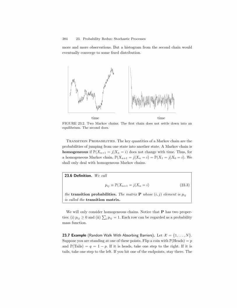
384 23. Probability Redux: Stochastic Processes
more and more observations. But a histogram from the second chain wouldeventually converge to some fixed distribution.
time timeFIGURE 23.2. Two Markov chains. The first chain does not settle down into anequilibrium. The second does.
Transition Probabilities. The key quantities of a Markov chain are theprobabilities of jumping from one state into another state. A Markov chain ishomogeneous if P(Xn+1 = j|Xn = i) does not change with time. Thus, fora homogeneous Markov chain, P(Xn+1 = j|Xn = i) = P(X1 = j|X0 = i). Weshall only deal with homogeneous Markov chains.
23.6 Definition. We call
pij 0 P(Xn+1 = j|Xn = i) (23.3)
the transition probabilities. The matrix P whose (i, j) element is pij
is called the transition matrix.
We will only consider homogeneous chains. Notice that P has two proper-ties: (i) pij * 0 and (ii)
0i pij = 1. Each row can be regarded as a probability
mass function.
23.7 Example (Random Walk With Absorbing Barriers). Let X = {1, . . . , N}.Suppose you are standing at one of these points. Flip a coin with P(Heads) = p
and P(Tails) = q = 1 " p. If it is heads, take one step to the right. If it istails, take one step to the left. If you hit one of the endpoints, stay there. The
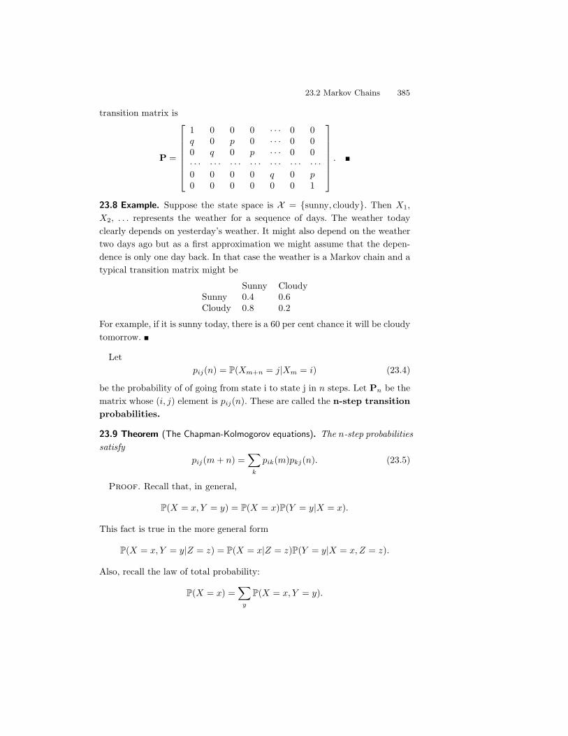
23.2 Markov Chains 385
transition matrix is
P =
N
OOOOOOP
1 0 0 0 · · · 0 0q 0 p 0 · · · 0 00 q 0 p · · · 0 0· · · · · · · · · · · · · · · · · · · · ·0 0 0 0 q 0 p0 0 0 0 0 0 1
Q
RRRRRRS. !
23.8 Example. Suppose the state space is X = {sunny, cloudy}. Then X1,X2, . . . represents the weather for a sequence of days. The weather todayclearly depends on yesterday’s weather. It might also depend on the weathertwo days ago but as a first approximation we might assume that the depen-dence is only one day back. In that case the weather is a Markov chain and atypical transition matrix might be
Sunny CloudySunny 0.4 0.6Cloudy 0.8 0.2
For example, if it is sunny today, there is a 60 per cent chance it will be cloudytomorrow. !
Letpij(n) = P(Xm+n = j|Xm = i) (23.4)
be the probability of of going from state i to state j in n steps. Let Pn be thematrix whose (i, j) element is pij(n). These are called the n-step transitionprobabilities.
23.9 Theorem (The Chapman-Kolmogorov equations). The n-step probabilitiessatisfy
pij(m + n) =*
k
pik(m)pkj(n). (23.5)
Proof. Recall that, in general,
P(X = x, Y = y) = P(X = x)P(Y = y|X = x).
This fact is true in the more general form
P(X = x, Y = y|Z = z) = P(X = x|Z = z)P(Y = y|X = x, Z = z).
Also, recall the law of total probability:
P(X = x) =*
y
P(X = x, Y = y).
386 23. Probability Redux: Stochastic Processes
Using these facts and the Markov property we have
pij(m + n) = P(Xm+n = j|X0 = i)
=*
k
P(Xm+n = j, Xm = k|X0 = i)
=*
k
P(Xm+n = j|Xm = k, X0 = i)P(Xm = k|X0 = i)
=*
k
P(Xm+n = j|Xm = k)P(Xm = k|X0 = i)
=*
k
pik(m)pkj(n). !
Look closely at equation (23.5). This is nothing more than the equation formatrix multiplication. Hence we have shown that
Pm+n = PmPn. (23.6)
By definition, P1 = P. Using the above theorem, P2 = P1+1 = P1P1 =PP = P2. Continuing this way, we see that
Pn = Pn 0 P-P- · · ·-Pa b_ `multiply the matrix n times
. (23.7)
Let µn = (µn(1), . . . , µn(N)) be a row vector where
µn(i) = P(Xn = i) (23.8)
is the marginal probability that the chain is in state i at time n. In particular,µ0 is called the initial distribution. To simulate a Markov chain, all youneed to know is µ0 and P. The simulation would look like this:
Step 1: Draw X0 ! µ0. Thus, P(X0 = i) = µ0(i).Step 2: Denote the outcome of step 1 by i. Draw X1 ! P. In other words,P(X1 = j|X0 = i) = pij .Step 3: Suppose the outcome of step 2 is j. Draw X2 ! P. In other words,P(X2 = k|X1 = j) = pjk.
And so on.
It might be di#cult to understand the meaning of µn. Imagine simulatingthe chain many times. Collect all the outcomes at time n from all the chains.This histogram would look approximately like µn. A consequence of theorem23.9 is the following:
23.2 Markov Chains 387
23.10 Lemma. The marginal probabilities are given by
µn = µ0Pn.
Proof.
µn(j) = P(Xn = j)
=*
i
P(Xn = j|X0 = i)P (X0 = i)
=*
i
µ0(i)pij(n) = µ0Pn. !
Summary of Terminology
1. Transition matrix: P(i, j) = P(Xn+1 = j|Xn = i) = pij .
2. n-step matrix: Pn(i, j) = P(Xn+m = j|Xm = i).
3. Pn = Pn.
4. Marginal: µn(i) = P(Xn = i).
5. µn = µ0Pn.
States. The states of a Markov chain can be classified according to variousproperties.
23.11 Definition. We say that i reaches j (or j is accessible from i) ifpij(n) > 0 for some n, and we write i) j. If i) j and j ) i then wewrite i2 j and we say that i and j communicate.
23.12 Theorem. The communication relation satisfies the following proper-ties:
1. i2 i.
2. If i2 j then j 2 i.
3. If i2 j and j 2 k then i2 k.
4. The set of states X can be written as a disjoint union of classes X =X1&X2&· · · where two states i and j communicate with each other if
and only if they are in the same class.
388 23. Probability Redux: Stochastic Processes
If all states communicate with each other, then the chain is called irre-ducible. A set of states is closed if, once you enter that set of states younever leave. A closed set consisting of a single state is called an absorbingstate.
23.13 Example. Let X = {1, 2, 3, 4} and
P =
E
FFFFG
13
23 0 0
23
13 0 0
14
14
14
14
0 0 0 1
H
IIIIJ
The classes are {1, 2}, {3} and {4}. State 4 is an absorbing state. !
Suppose we start a chain in state i. Will the chain ever return to state i?If so, that state is called persistent or recurrent.
23.14 Definition. State i is recurrent or persistent if
P(Xn = i for some n * 1 | X0 = i) = 1.
Otherwise, state i is transient.
23.15 Theorem. A state i is recurrent if and only if*
n
pii(n) =#. (23.9)
A state i is transient if and only if*
n
pii(n) <#. (23.10)
Proof. DefineIn =
'1 if Xn = i0 if Xn (= i.
The number of times that the chain is in state i is Y =0!
n=0 In. The meanof Y , given that the chain starts in state i, is
E(Y |X0 = i) =!*
n=0
E(In|X0 = i) =!*
n=0
P(Xn = i|X0 = i) =!*
n=0
pii(n).
Define ai = P(Xn = i for some n * 1 | X0 = i). If i is recurrent, ai = 1. Thus,the chain will eventually return to i. Once it does return to i, we argue again
23.2 Markov Chains 389
that since ai = 1, the chain will return to state i again. By repeating thisargument, we conclude that E(Y |X0 = i) = #. If i is transient, then ai < 1.When the chain is in state i, there is a probability 1"ai > 0 that it will neverreturn to state i. Thus, the probability that the chain is in state i exactly n
times is an$1i (1" ai). This is a geometric distribution which has finite mean.
!
23.16 Theorem. Facts about recurrence.
1. If state i is recurrent and i2 j, then j is recurrent.
2. If state i is transient and i2 j, then j is transient.
3. A finite Markov chain must have at least one recurrent state.
4. The states of a finite, irreducible Markov chain are all recurrent.
23.17 Theorem (Decomposition Theorem). The state space X can be writtenas the disjoint union
X = XT
#X1
#X2 · · ·
where XT are the transient states and each Xi is a closed, irreducible set ofrecurrent states.
23.18 Example (Random Walk). Let X = {. . . ,"2,"1, 0, 1, 2, . . . , } and sup-pose that pi,i+1 = p, pi,i$1 = q = 1" p. All states communicate, hence eitherall the states are recurrent or all are transient. To see which, suppose we startat X0 = 0. Note that
p00(2n) =-
2n
n
.pnqn (23.11)
since the only way to get back to 0 is to have n heads (steps to the right) andn tails (steps to the left). We can approximate this expression using Stirling’sformula which says that
n! ! nn/ne$n/
2&.
Inserting this approximation into (23.11) shows that
p00(2n) ! (4pq)n
/n&
.
It is easy to check that0
n p00(n) < # if and only if0
n p00(2n) < #.Moreover,
0n p00(2n) = # if and only if p = q = 1/2. By Theorem (23.15),
the chain is recurrent if p = 1/2 otherwise it is transient. !
390 23. Probability Redux: Stochastic Processes
Convergence of Markov Chains. To discuss the convergence of chains,we need a few more definitions. Suppose that X0 = i. Define the recurrencetime
Tij = min{n > 0 : Xn = j} (23.12)
assuming Xn ever returns to state i, otherwise define Tij = #. The meanrecurrence time of a recurrent state i is
mi = E(Tii) =*
n
nfii(n) (23.13)
where
fij(n) = P(X1 (= j, X2 (= j, . . . , Xn$1 (= j, Xn = j|X0 = i).
A recurrent state is null if mi = # otherwise it is called non-null or posi-tive.
23.19 Lemma. If a state is null and recurrent, then pnii ) 0.
23.20 Lemma. In a finite state Markov chain, all recurrent states are positive.
Consider a three-state chain with transition matrixN
P0 1 00 0 11 0 0
Q
S .
Suppose we start the chain in state 1. Then we will be in state 3 at times 3, 6,9, . . . . This is an example of a periodic chain. Formally, the period of state i
is d if pii(n) = 0 whenever n is not divisible by d and d is the largest integerwith this property. Thus, d = gcd{n : pii(n) > 0} where gcd means “greatercommon divisor.” State i is periodic if d(i) > 1 and aperiodic if d(i) = 1.A state with period 1 is called aperiodic.
23.21 Lemma. If state i has period d and i2 j then j has period d.
23.22 Definition. A state is ergodic if it is recurrent, non-null andaperiodic. A chain is ergodic if all its states are ergodic.
Let & = (&i : i $ X ) be a vector of non-negative numbers that sum to one.Thus & can be thought of as a probability mass function.
23.23 Definition. We say that & is a stationary (or invariant)distribution if & = &P.
23.2 Markov Chains 391
Here is the intuition. Draw X0 from distribution & and suppose that & is astationary distribution. Now draw X1 according to the transition probabilityof the chain. The distribution of X1 is then µ1 = µ0P = &P = &. Thedistribution of X2 is &P2 = (&P)P = &P = &. Continuing this way, we seethat the distribution of Xn is &Pn = &. In other words:
If at any time the chain has distribution &, then it will continue to
have distribution & forever.
23.24 Definition. We say that a chain has limiting distribution if
Pn )
N
OOOP
&&...&
Q
RRRS
for some &, that is, &j = limn"! Pnij exists and is independent of i.
Here is the main theorem about convergence. The theorem says that anergodic chain converges to its stationary distribution. Also, sample averagesconverge to their theoretical expectations under the stationary distribution.
23.25 Theorem. An irreducible, ergodic Markov chain has a uniquestationary distribution &. The limiting distribution exists and is equal to&. If g is any bounded function, then, with probability 1,
limN"!
1N
N*
n=1
g(Xn)) E-(g) 0*
j
g(j)&j . (23.14)
Finally, there is another definition that will be useful later. We say that &satisfies detailed balance if
&ipij = pji&j . (23.15)
Detailed balance guarantees that & is a stationary distribution.
23.26 Theorem. If & satisfies detailed balance, then & is a stationary distri-bution.
Proof. We need to show that &P = &. The jth element of &P is0
i &ipij =0i &jpji = &j
0i pji = &j . !
392 23. Probability Redux: Stochastic Processes
The importance of detailed balance will become clear when we discussMarkov chain Monte Carlo methods in Chapter 24.
Warning! Just because a chain has a stationary distribution does not meanit converges.
23.27 Example. Let
P =
N
P0 1 00 0 11 0 0
Q
S .
Let & = (1/3, 1/3, 1/3). Then &P = & so & is a stationary distribution. Ifthe chain is started with the distribution & it will stay in that distribution.Imagine simulating many chains and checking the marginal distribution ateach time n. It will always be the uniform distribution &. But this chain doesnot have a limit. It continues to cycle around forever. !
Examples of Markov Chains.
23.28 Example. Let X = {1, 2, 3, 4, 5, 6}. Let
P =
N
OOOOOOOOOP
12
12 0 0 0 0
14
34 0 0 0 0
14
14
14
14 0 0
14 0 1
414 0 1
4
0 0 0 0 12
12
0 0 0 0 12
12
Q
RRRRRRRRRS
Then C1 = {1, 2} and C2 = {5, 6} are irreducible closed sets. States 3 and4 are transient because of the path 3 ) 4 ) 6 and once you hit state 6you cannot return to 3 or 4. Since pii(1) > 0, all the states are aperiodic. Insummary, 3 and 4 are transient while 1, 2, 5, and 6 are ergodic. !
23.29 Example (Hardy-Weinberg). Here is a famous example from genetics.Suppose a gene can be type A or type a. There are three types of people (calledgenotypes): AA, Aa, and aa. Let (p, q, r) denote the fraction of people of eachgenotype. We assume that everyone contributes one of their two copies of thegene at random to their children. We also assume that mates are selected atrandom. The latter is not realistic however, it is often reasonable to assumethat you do not choose your mate based on whether they are AA, Aa, oraa. (This would be false if the gene was for eye color and if people chosemates based on eye color.) Imagine if we pooled everyone’s genes together.The proportion of A genes is P = p + (q/2) and the proportion of a genes is
23.2 Markov Chains 393
Q = r + (q/2). A child is AA with probability P 2, aA with probability 2PQ,and aa with probability Q2. Thus, the fraction of A genes in this generationis
P 2 + PQ =+p +
q
2
,2++p +
q
2
,+r +
q
2
,.
However, r = 1 " p " q. Substitute this in the above equation and you getP 2 + PQ = P . A similar calculation shows that the fraction of “a” genes isQ. We have shown that the proportion of type A and type a is P and Q andthis remains stable after the first generation. The proportion of people of typeAA, Aa, aa is thus (P 2, 2PQ, Q2) from the second generation and on. This iscalled the Hardy-Weinberg law.
Assume everyone has exactly one child. Now consider a fixed person andlet Xn be the genotype of their nth descendant. This is a Markov chain withstate space X = {AA, Aa, aa}. Some basic calculations will show you that thetransition matrix is N
PP Q 0P2
P+Q2
Q2
0 P Q
Q
S .
The stationary distribution is & = (P 2, 2PQ, Q2). !
23.30 Example (Markov chain Monte Carlo). In Chapter 24 we will present asimulation method called Markov chain Monte Carlo (MCMC). Here is a briefdescription of the idea. Let f(x) be a probability density on the real line andsuppose that f(x) = cg(x) where g(x) is a known function and c > 0 isunknown. In principle, we can compute c since
8f(x)dx = 1 implies that
c = 1/8
g(x)dx. However, it may not be feasible to perform this integral, noris it necessary to know c in the following algorithm. Let X0 be an arbitrarystarting value. Given X0, . . . , Xi, draw Xi+1 as follows. First, draw W !N(Xi, b2) where b > 0 is some fixed constant. Let
r = min'
g(W )g(Xi)
, 12
.
Draw U ! Uniform(0, 1) and set
Xi+1 ='
W if U < rXi if U * r.
We will see in Chapter 24 that, under weak conditions, X0, X1, . . . , is anergodic Markov chain with stationary distribution f . Hence, we can regardthe draws as a sample from f . !
394 23. Probability Redux: Stochastic Processes
Inference for Markov Chains. Consider a chain with finite state spaceX = {1, 2, . . . , N}. Suppose we observe n observations X1, . . . , Xn from thischain. The unknown parameters of a Markov chain are the initial probabilitiesµ0 = (µ0(1), µ0(2), . . . , ) and the elements of the transition matrix P. Eachrow of P is a multinomial distribution. So we are essentially estimating N
distributions (plus the initial probabilities). Let nij be the observed numberof transitions from state i to state j. The likelihood function is
L(µ0,P) = µ0(x0)n/
r=1
pXr#1,Xr = µ0(x0)N/
i=1
N/
j=1
pnij
ij .
There is only one observation on µ0 so we can’t estimate that. Rather, wefocus on estimating P. The mle is obtained by maximizing L(µ0,P) subjectto the constraint that the elements are non-negative and the rows sum to 1.The solution is
1pij =nij
ni
where ni =0N
j=1 nij . Here we are assuming that ni > 0. If not, then we set1pij = 0 by convention.
23.31 Theorem (Consistency and Asymptotic Normality of the mle). Assume thatthe chain is ergodic. Let 1pij(n) denote the mle after n observations. Then1pij(n) P") pij. Also,
?3Ni(n)(1pij " pij)
@! N(0,')
where the left-hand side is a matrix, Ni(n) =0n
r=1 I(Xr = i) and
'ij,k. =
46
7
pij(1 " pij) (i, j) = (k, 4)"pijpi. i = k, j (= 40 otherwise.
23.3 Poisson Processes
The Poisson process arises when we count occurrences of events over time, forexample, tra#c accidents, radioactive decay, arrival of email messages, etc.As the name suggests, the Poisson process is intimately related to the Poissondistribution. Let’s first review the Poisson distribution.
Recall that X has a Poisson distribution with parameter % — written X !Poisson(%) — if
P(X = x) 0 p(x; %) =e$!%x
x!, x = 0, 1, 2, . . .
23.3 Poisson Processes 395
Also recall that E(X) = % and V(X) = %. If X ! Poisson(%), Y ! Poisson(*)and X!Y , then X+Y ! Poisson(%+*). Finally, if N ! Poisson(%) and Y |N =n ! Binomial(n, p), then the marginal distribution of Y is Y ! Poisson(%p).
Now we describe the Poisson process. Imagine that you are at your com-puter. Each time a new email message arrives you record the time. Let Xt bethe number of messages you have received up to and including time t. Then,{Xt : t $ [0,#)} is a stochastic process with state space X = {0, 1, 2, . . .}.A process of this form is called a counting process. A Poisson process isa counting process that satisfies certain conditions. In what follows, we willsometimes write X(t) instead of Xt. Also, we need the following notation.Write f(h) = o(h) if f(h)/h ) 0 as h ) 0. This means that f(h) is smallerthan h when h is close to 0. For example, h2 = o(h).
23.32 Definition. A Poisson process is a stochastic process{Xt : t $ [0,#)} with state space X = {0, 1, 2, . . .} such that
1. X(0) = 0.
2. For any 0 = t0 < t1 < t2 < · · · < tn, the increments
X(t1)"X(t0), X(t2)"X(t1), · · · , X(tn)"X(tn$1)
are independent.
3. There is a function %(t) such that
P(X(t + h)"X(t) = 1) = %(t)h + o(h) (23.16)
P(X(t + h)"X(t) * 2) = o(h). (23.17)
We call %(t) the intensity function.
The last condition means that the probability of an event in [t, t + h] isapproximately h%(t) while the probability of more than one event is small.
23.33 Theorem. If Xt is a Poisson process with intensity function %(t), then
X(s + t)"X(s) ! Poisson(m(s + t)"m(s))
where
m(t) =9 t
0%(s) ds.
In particular, X(t) ! Poisson(m(t)). Hence, E(X(t)) = m(t) and V(X(t)) =m(t).
396 23. Probability Redux: Stochastic Processes
23.34 Definition. A Poisson process with intensity function %(t) 0 % forsome % > 0 is called a homogeneous Poisson process with rate %. Inthis case,
X(t) ! Poisson(%t).
Let X(t) be a homogeneous Poisson process with rate %. Let Wn be thetime at which the nth event occurs and set W0 = 0. The random variablesW0, W1, . . . , are called waiting times. Let Sn = Wn+1"Wn. Then S0, S1, . . . ,
are called sojourn times or interarrival times.
23.35 Theorem. The sojourn times S0, S1, . . . are iid random variables. Theirdistribution is exponential with mean 1/%, that is, they have density
f(s) = %e$!s, s * 0.
The waiting time Wn ! Gamma(n, 1/%) i.e., it has density
f(w) =1
&(n)%nwn$1e$!t.
Hence, E(Wn) = n/% and V(Wn) = n/%2.
Proof. First, we have
P(S1 > t) = P(X(t) = 0) = e$!t
with shows that the cdf for S1 is 1"e$!t. This shows the result for S1. Now,
P(S2 > t|S1 = s) = P(no events in (s, s + t]|S1 = s)
= P(no events in (s, s + t]) (increments are independent)
= e$!t.
Hence, S2 has an exponential distribution and is independent of S1. The resultfollows by repeating the argument. The result for Wn follows since a sum ofexponentials has a Gamma distribution. !
23.36 Example. Figure 23.3 shows requests to a WWW server in Calgary.1
Assuming that this is a homogeneous Poisson process, N 0 X(T ) ! Poisson(%T ).The likelihood is
L(%) 3 e$!T (%T )N
1See http://ita.ee.lbl.gov/html/contrib/Calgary-HTTP.html for more information.
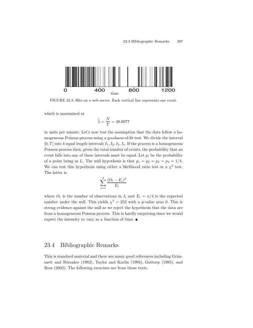
23.4 Bibliographic Remarks 397
0 400 800 1200time
FIGURE 23.3. Hits on a web server. Each vertical line represents one event.
which is maximized at
1% =N
T= 48.0077
in units per minute. Let’s now test the assumption that the data follow a ho-mogeneous Poisson process using a goodness-of-fit test. We divide the interval[0, T ] into 4 equal length intervals I1, I2, I3, I4. If the process is a homogeneousPoisson process then, given the total number of events, the probability that anevent falls into any of these intervals must be equal. Let pi be the probabilityof a point being in Ii. The null hypothesis is that p1 = p2 = p3 = p4 = 1/4.We can test this hypothesis using either a likelihood ratio test or a !2 test.The latter is
4*
i=1
(Oi " Ei)2
Ei
where Oi is the number of observations in Ii and Ei = n/4 is the expectednumber under the null. This yields !2 = 252 with a p-value near 0. This isstrong evidence against the null so we reject the hypothesis that the data arefrom a homogeneous Poisson process. This is hardly surprising since we wouldexpect the intensity to vary as a function of time. !
23.4 Bibliographic Remarks
This is standard material and there are many good references including Grim-mett and Stirzaker (1982), Taylor and Karlin (1994), Guttorp (1995), andRoss (2002). The following exercises are from those texts.
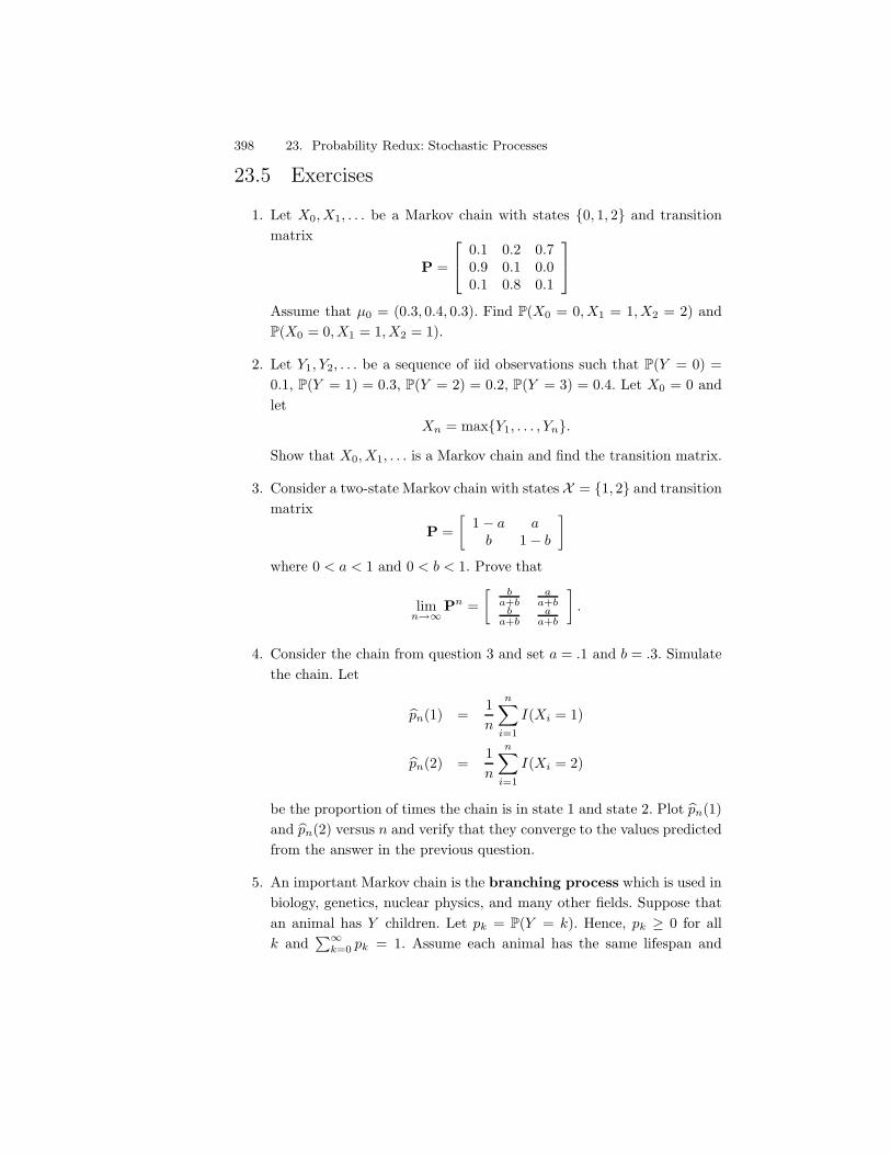
398 23. Probability Redux: Stochastic Processes
23.5 Exercises
1. Let X0, X1, . . . be a Markov chain with states {0, 1, 2} and transitionmatrix
P =
N
P0.1 0.2 0.70.9 0.1 0.00.1 0.8 0.1
Q
S
Assume that µ0 = (0.3, 0.4, 0.3). Find P(X0 = 0, X1 = 1, X2 = 2) andP(X0 = 0, X1 = 1, X2 = 1).
2. Let Y1, Y2, . . . be a sequence of iid observations such that P(Y = 0) =0.1, P(Y = 1) = 0.3, P(Y = 2) = 0.2, P(Y = 3) = 0.4. Let X0 = 0 andlet
Xn = max{Y1, . . . , Yn}.
Show that X0, X1, . . . is a Markov chain and find the transition matrix.
3. Consider a two-state Markov chain with states X = {1, 2} and transitionmatrix
P =A
1" a ab 1" b
B
where 0 < a < 1 and 0 < b < 1. Prove that
limn"!
Pn =A b
a+ba
a+bb
a+ba
a+b
B.
4. Consider the chain from question 3 and set a = .1 and b = .3. Simulatethe chain. Let
1pn(1) =1n
n*
i=1
I(Xi = 1)
1pn(2) =1n
n*
i=1
I(Xi = 2)
be the proportion of times the chain is in state 1 and state 2. Plot 1pn(1)and 1pn(2) versus n and verify that they converge to the values predictedfrom the answer in the previous question.
5. An important Markov chain is the branching process which is used inbiology, genetics, nuclear physics, and many other fields. Suppose thatan animal has Y children. Let pk = P(Y = k). Hence, pk * 0 for allk and
0!k=0 pk = 1. Assume each animal has the same lifespan and
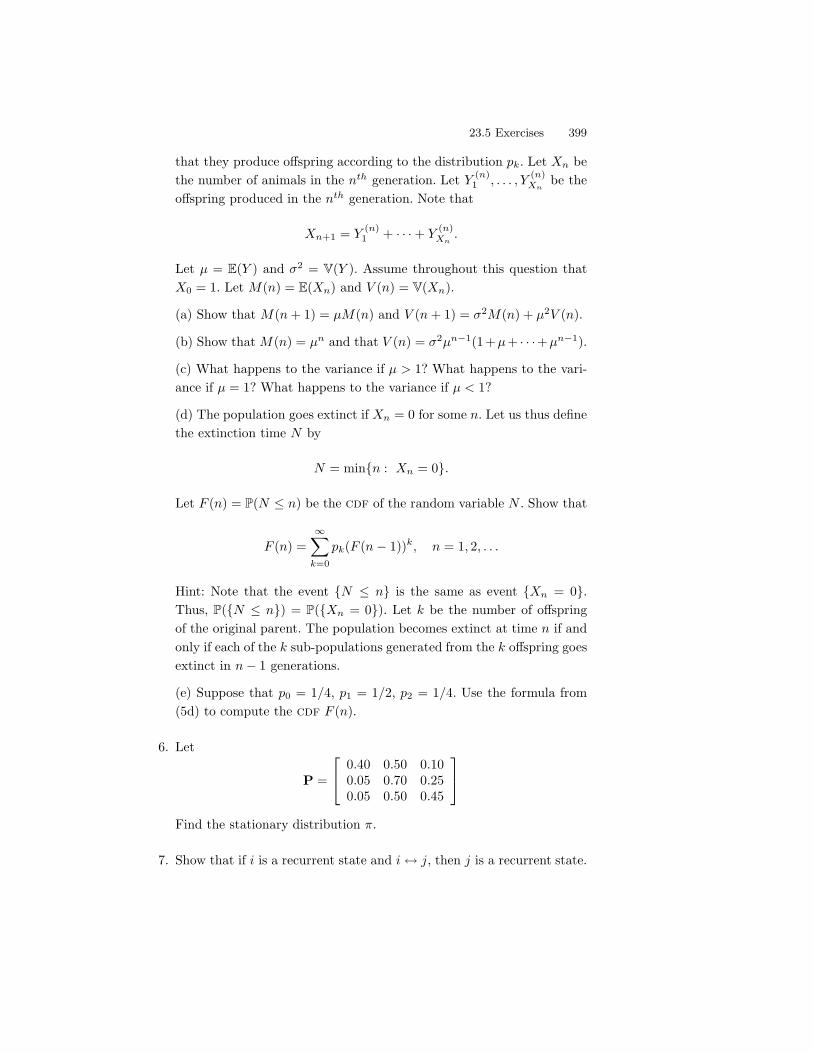
23.5 Exercises 399
that they produce o!spring according to the distribution pk. Let Xn bethe number of animals in the nth generation. Let Y (n)
1 , . . . , Y (n)Xn
be theo!spring produced in the nth generation. Note that
Xn+1 = Y (n)1 + · · · + Y (n)
Xn.
Let µ = E(Y ) and #2 = V(Y ). Assume throughout this question thatX0 = 1. Let M(n) = E(Xn) and V (n) = V(Xn).
(a) Show that M(n + 1) = µM(n) and V (n + 1) = #2M(n) + µ2V (n).
(b) Show that M(n) = µn and that V (n) = #2µn$1(1+µ+ · · ·+µn$1).
(c) What happens to the variance if µ > 1? What happens to the vari-ance if µ = 1? What happens to the variance if µ < 1?
(d) The population goes extinct if Xn = 0 for some n. Let us thus definethe extinction time N by
N = min{n : Xn = 0}.
Let F (n) = P(N , n) be the cdf of the random variable N . Show that
F (n) =!*
k=0
pk(F (n" 1))k, n = 1, 2, . . .
Hint: Note that the event {N , n} is the same as event {Xn = 0}.Thus, P({N , n}) = P({Xn = 0}). Let k be the number of o!springof the original parent. The population becomes extinct at time n if andonly if each of the k sub-populations generated from the k o!spring goesextinct in n" 1 generations.
(e) Suppose that p0 = 1/4, p1 = 1/2, p2 = 1/4. Use the formula from(5d) to compute the cdf F (n).
6. Let
P =
N
P0.40 0.50 0.100.05 0.70 0.250.05 0.50 0.45
Q
S
Find the stationary distribution &.
7. Show that if i is a recurrent state and i2 j, then j is a recurrent state.
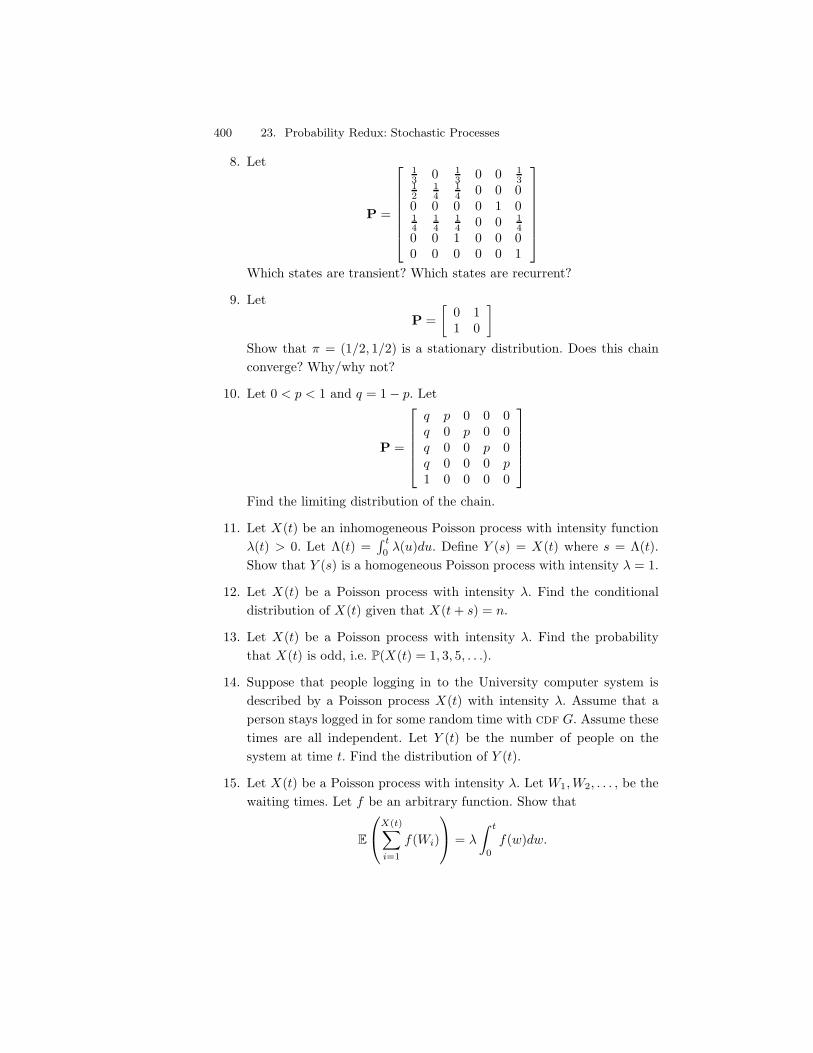
400 23. Probability Redux: Stochastic Processes
8. Let
P =
N
OOOOOOP
13 0 1
3 0 0 13
12
14
14 0 0 0
0 0 0 0 1 014
14
14 0 0 1
40 0 1 0 0 00 0 0 0 0 1
Q
RRRRRRS
Which states are transient? Which states are recurrent?
9. LetP =
A0 11 0
B
Show that & = (1/2, 1/2) is a stationary distribution. Does this chainconverge? Why/why not?
10. Let 0 < p < 1 and q = 1" p. Let
P =
N
OOOOP
q p 0 0 0q 0 p 0 0q 0 0 p 0q 0 0 0 p1 0 0 0 0
Q
RRRRS
Find the limiting distribution of the chain.
11. Let X(t) be an inhomogeneous Poisson process with intensity function%(t) > 0. Let *(t) =
8 t0 %(u)du. Define Y (s) = X(t) where s = *(t).
Show that Y (s) is a homogeneous Poisson process with intensity % = 1.
12. Let X(t) be a Poisson process with intensity %. Find the conditionaldistribution of X(t) given that X(t + s) = n.
13. Let X(t) be a Poisson process with intensity %. Find the probabilitythat X(t) is odd, i.e. P(X(t) = 1, 3, 5, . . .).
14. Suppose that people logging in to the University computer system isdescribed by a Poisson process X(t) with intensity %. Assume that aperson stays logged in for some random time with cdf G. Assume thesetimes are all independent. Let Y (t) be the number of people on thesystem at time t. Find the distribution of Y (t).
15. Let X(t) be a Poisson process with intensity %. Let W1, W2, . . . , be thewaiting times. Let f be an arbitrary function. Show that
E
E
GX(t)*
i=1
f(Wi)
H
J = %
9 t
0f(w)dw.
23.5 Exercises 401
16. A two-dimensional Poisson point process is a process of random pointson the plane such that (i) for any set A, the number of points fallingin A is Poisson with mean %µ(A) where µ(A) is the area of A, (ii) thenumber of events in non-overlapping regions is independent. Consideran arbitrary point x0 in the plane. Let X denote the distance from x0
to the nearest random point. Show that
P(X > t) = e$!-t2
andE(X) =
12/%
.

This is page 402Printer: Opaque this
This is page 403Printer: Opaque this
24Simulation Methods
In this chapter we will show how simulation can be used to approximate inte-grals. Our leading example is the problem of computing integrals in Bayesianinference but the techniques are widely applicable. We will look at three inte-gration methods: (i) basic Monte Carlo integration, (ii) importance sampling,and (iii) Markov chain Monte Carlo (MCMC).
24.1 Bayesian Inference Revisited
Simulation methods are especially useful in Bayesian inference so let us brieflyreview the main ideas in Bayesian inference. See Chapter 11 for more details.
Given a prior f(0) and data Xn = (X1, . . . , Xn) the posterior density is
f(0|Xn) =L(0)f(0)
c
where L(0) is the likelihood function and
c =9
L(0)f(0) d0
is the normalizing constant. The posterior mean is
0 =90f(0|Xn)d0 =
80L(0)f(0)d0
c.
404 24. Simulation Methods
If 0 = (01, . . . , 0k) is multidimensional, then we might be interested in theposterior for one of the components, 01, say. This marginal posterior densityis
f(01|Xn) =9 9
· · ·9
f(01, . . . , 0k|Xn)d02 · · · d0k
which involves high-dimensional integration.When 0 is high-dimensional, it may not be feasible to calculate these inte-
grals analytically. Simulation methods will often be helpful.
24.2 Basic Monte Carlo Integration
Suppose we want to evaluate the integral
I =9 b
ah(x) dx
for some function h. If h is an “easy” function like a polynomial or trigono-metric function, then we can do the integral in closed form. If h is complicatedthere may be no known closed form expression for I. There are many numer-ical techniques for evaluating I such as Simpson’s rule, the trapezoidal ruleand Gaussian quadrature. Monte Carlo integration is another approach forapproximating I which is notable for its simplicity, generality and scalability.
Let us begin by writing
I =9 b
ah(x)dx =
9 b
aw(x)f(x)dx (24.1)
where w(x) = h(x)(b"a) and f(x) = 1/(b"a). Notice that f is the probabilitydensity for a uniform random variable over (a, b). Hence,
I = Ef (w(X))
where X ! Unif(a, b). If we generate X1, . . . , XN ! Unif(a, b), then by thelaw of large numbers
1I 0 1N
N*
i=1
w(Xi)P")E(w(X)) = I. (24.2)
This is the basic Monte Carlo integration method. We can also computethe standard error of the estimate
1se =s/N
24.2 Basic Monte Carlo Integration 405
where
s2 =0N
i=1(Yi " 1I)2
N " 1
where Yi = w(Xi). A 1") confidence interval for I is 1I ±z#/2 1se. We can takeN as large as we want and hence make the length of the confidence intervalvery small.
24.1 Example. Let h(x) = x3. Then, I =8 10 x3dx = 1/4. Based on N =
10, 000 observations from a Uniform(0, 1) we get 1I = .248 with a standarderror of .0028. !
A generalization of the basic method is to consider integrals of the form
I =9
h(x)f(x)dx (24.3)
where f(x) is a probability density function. Taking f to be a Uniform (a,b)gives us the special case above. Now we draw X1, . . . , XN ! f and take
1I 0 1N
N*
i=1
h(Xi)
as before.
24.2 Example. Let
f(x) =1/2&
e$x2/2
be the standard Normal pdf. Suppose we want to compute the cdf at somepoint x:
I =9 x
$!f(s)ds = %(x).
WriteI =
9h(s)f(s)ds
whereh(s) =
'1 s < x0 s * x.
Now we generate X1, . . . , XN ! N(0, 1) and set
1I =1N
*
i
h(Xi) =number of observations , x
N.
For example, with x = 2, the true answer is %(2) = .9772 and the MonteCarlo estimate with N = 10, 000 yields .9751. Using N = 100, 000 we get.9771. !
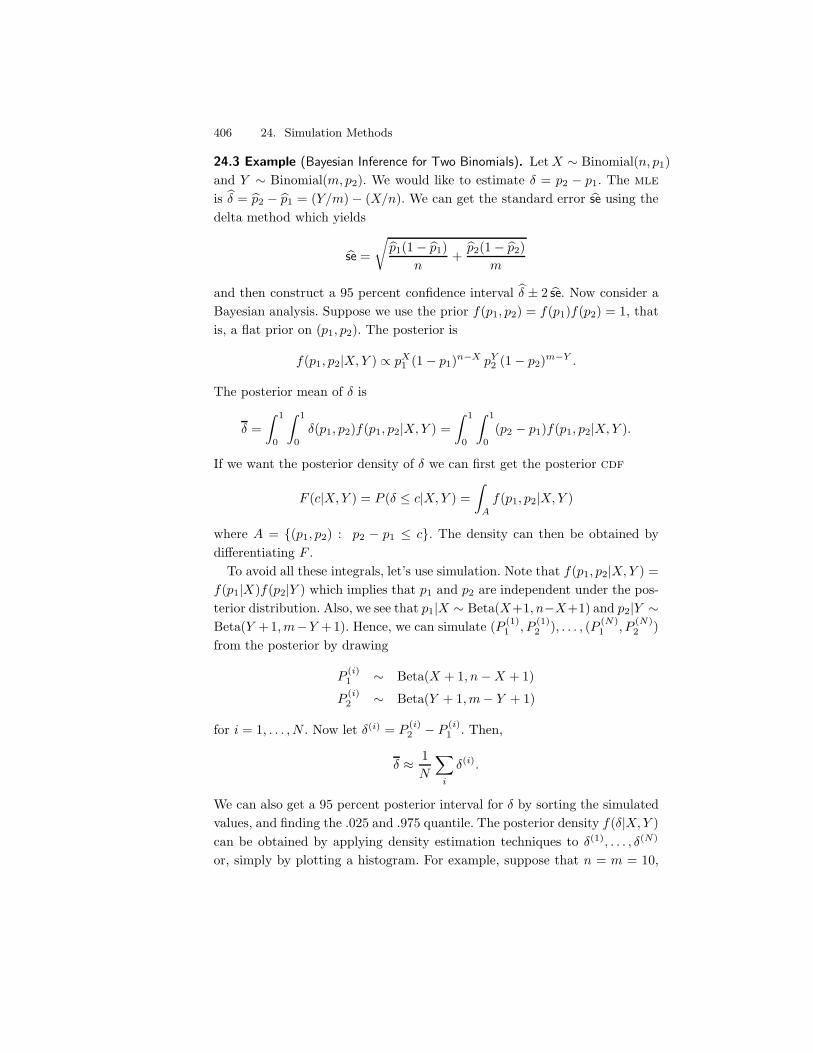
406 24. Simulation Methods
24.3 Example (Bayesian Inference for Two Binomials). Let X ! Binomial(n, p1)and Y ! Binomial(m, p2). We would like to estimate $ = p2 " p1. The mle
is 1$ = 1p2 " 1p1 = (Y/m)" (X/n). We can get the standard error 1se using thedelta method which yields
1se =
U1p1(1" 1p1)
n+1p2(1" 1p2)
m
and then construct a 95 percent confidence interval 1$ ± 2 1se. Now consider aBayesian analysis. Suppose we use the prior f(p1, p2) = f(p1)f(p2) = 1, thatis, a flat prior on (p1, p2). The posterior is
f(p1, p2|X, Y ) 3 pX1 (1" p1)n$X pY
2 (1 " p2)m$Y .
The posterior mean of $ is
$ =9 1
0
9 1
0$(p1, p2)f(p1, p2|X, Y ) =
9 1
0
9 1
0(p2 " p1)f(p1, p2|X, Y ).
If we want the posterior density of $ we can first get the posterior cdf
F (c|X, Y ) = P ($ , c|X, Y ) =9
Af(p1, p2|X, Y )
where A = {(p1, p2) : p2 " p1 , c}. The density can then be obtained bydi!erentiating F .
To avoid all these integrals, let’s use simulation. Note that f(p1, p2|X, Y ) =f(p1|X)f(p2|Y ) which implies that p1 and p2 are independent under the pos-terior distribution. Also, we see that p1|X ! Beta(X+1, n"X+1) and p2|Y !Beta(Y +1, m"Y +1). Hence, we can simulate (P (1)
1 , P (1)2 ), . . . , (P (N)
1 , P (N)2 )
from the posterior by drawing
P (i)1 ! Beta(X + 1, n"X + 1)
P (i)2 ! Beta(Y + 1, m" Y + 1)
for i = 1, . . . , N . Now let $(i) = P (i)2 " P (i)
1 . Then,
$ . 1N
*
i
$(i).
We can also get a 95 percent posterior interval for $ by sorting the simulatedvalues, and finding the .025 and .975 quantile. The posterior density f($|X, Y )can be obtained by applying density estimation techniques to $(1), . . . , $(N)
or, simply by plotting a histogram. For example, suppose that n = m = 10,
24.2 Basic Monte Carlo Integration 407
!0.6 0.0 0.6
FIGURE 24.1. Posterior of ' from simulation.
X = 8 and Y = 6. From a posterior sample of size 1000 we get a 95 percentposterior interval of (-0.52,0.20). The posterior density can be estimated froma histogram of the simulated values as shown in Figure 24.1. !
24.4 Example (Bayesian Inference for Dose Response). Suppose we conduct anexperiment by giving rats one of ten possible doses of a drug, denoted byx1 < x2 < . . . < x10. For each dose level xi we use n rats and we observeYi, the number that survive. Thus we have ten independent binomials Yi !Binomial(n, pi). Suppose we know from biological considerations that higherdoses should have higher probability of death. Thus, p1 , p2 , · · · , p10. Wewant to estimate the dose at which the animals have a 50 percent chance ofdying. This is called the LD50. Formally, $ = xj where
j = min{i : pi * .50}.
Notice that $ is implicitly a (complicated) function of p1, . . . , p10 so we canwrite $ = g(p1, . . . , p10) for some g. This just means that if we know (p1, . . . , p10)then we can find $. The posterior mean of $ is
9 9· · ·9
Ag(p1, . . . , p10)f(p1, . . . , p10|Y1, . . . , Y10)dp1dp2 . . . dp10.
The integral is over the region
A = {(p1, . . . , p10) : p1 , · · · , p10}.
The posterior cdf of $ is
F (c|Y1, . . . , Y10) = P($ , c|Y1, . . . , Y10)
=9 9
· · ·9
Bf(p1, . . . , p10|Y1, . . . , Y10)dp1dp2 . . . dp10
408 24. Simulation Methods
where
B = A$:
(p1, . . . , p10) : g(p1, . . . , p10) , c
Y.
We need to do a 10-dimensional integral over a restricted region A. Instead,we will use simulation. Let us take a flat prior truncated over A. Except forthe truncation, each Pi has once again a Beta distribution. To draw from theposterior we do the following steps:
(1) Draw Pi ! Beta(Yi + 1, n" Yi + 1), i = 1, . . . , 10.(2) If P1 , P2 , · · · , P10 keep this draw. Otherwise, throw it away and
draw again until you get one you can keep.(3) Let $ = xj where
j = min{i : Pi > .50}.
We repeat this N times to get $(1), . . . , $(N) and take
E($|Y1, . . . , Y10) .1N
*
i
$(i).
$ is a discrete variable. We can estimate its probability mass function by
P($ = xj |Y1, . . . , Y10) .1N
N*
i=1
I($(i) = j).
For example, consider the following data:
Dose 1 2 3 4 5 6 7 8 9 10Number of animals ni 15 15 15 15 15 15 15 15 15 15Number of survivors Yi 0 0 2 2 8 10 12 14 15 14
The posterior draws for p1, . . . , p10 are shown in the second panel in thefigure. We find that that $ = 4.04 with a 95 percent interval of (3,5). !
24.3 Importance Sampling
Consider again the integral I =8
h(x)f(x)dx where f is a probability density.The basic Monte Carlo method involves sampling from f . However, thereare cases where we may not know how to sample from f . For example, inBayesian inference, the posterior density density is is obtained by multiplyingthe likelihood L(0) times the prior f(0). There is no guarantee that f(0|x)will be a known distribution like a Normal or Gamma or whatever.
24.3 Importance Sampling 409
Importance sampling is a generalization of basic Monte Carlo which over-comes this problem. Let g be a probability density that we know how tosimulate from. Then
I =9
h(x)f(x)dx =9
h(x)f(x)g(x)
g(x)dx = Eg(Y ) (24.4)
where Y = h(X)f(X)/g(X) and the expectation Eg(Y ) is with respect to g.We can simulate X1, . . . , XN ! g and estimate I by
1I =1N
*
i
Yi =1N
*
i
h(Xi)f(Xi)g(Xi)
. (24.5)
This is called importance sampling. By the law of large numbers, 1I P") I.However, there is a catch. It’s possible that 1I might have an infinite standarderror. To see why, recall that I is the mean of w(x) = h(x)f(x)/g(x). Thesecond moment of this quantity is
Eg(w2(X)) =9 -
h(x)f(x)g(x)
.2
g(x)dx =9
h2(x)f2(x)g(x)
dx. (24.6)
If g has thinner tails than f , then this integral might be infinite. To avoid this,a basic rule in importance sampling is to sample from a density g with thickertails than f . Also, suppose that g(x) is small over some set A where f(x) islarge. Again, the ratio of f/g could be large leading to a large variance. Thisimplies that we should choose g to be similar in shape to f . In summary, agood choice for an importance sampling density g should be similar to f butwith thicker tails. In fact, we can say what the optimal choice of g is.
24.5 Theorem. The choice of g that minimizes the variance of 1I is
g*(x) =|h(x)|f(x)8|h(s)|f(s)ds
.
Proof. The variance of w = fh/g is
Eg(w2)" (E(w2))2 =9
w2(x)g(x)dx "-9
w(x)g(x)dx
.2
=9
h2(x)f2(x)g2(x)
g(x)dx "-9
h(x)f(x)g(x)
g(x)dx
.2
=9
h2(x)f2(x)g2(x)
g(x)dx "-9
h(x)f(x)dx
.2
.
410 24. Simulation Methods
The second integral does not depend on g, so we only need to minimize thefirst integral. From Jensen’s inequality (Theorem 4.9) we have
Eg(W 2) * (Eg(|W |))2 =-9
|h(x)|f(x)dx
.2
.
This establishes a lower bound on Eg(W 2). However, Eg$(W 2) equals thislower bound which proves the claim. !
This theorem is interesting but it is only of theoretical interest. If we didnot know how to sample from f then it is unlikely that we could sample from|h(x)|f(x)/
8|h(s)|f(s)ds. In practice, we simply try to find a thick-tailed
distribution g which is similar to f |h|.
24.6 Example (Tail Probability). Let’s estimate I = P(Z > 3) = .0013 whereZ ! N(0, 1). Write I =
8h(x)f(x)dx where f(x) is the standard Normal
density and h(x) = 1 if x > 3, and 0 otherwise. The basic Monte Carloestimator is 1I = N$1
0i h(Xi) where X1, . . . , XN ! N(0, 1). Using N = 100
we find (from simulating many times) that E(1I) = .0015 and V(1I) = .0039.Notice that most observations are wasted in the sense that most are not nearthe right tail. Now we will estimate this with importance sampling taking g
to be a Normal(4,1) density. We draw values from g and the estimate is now1I = N$1
0i f(Xi)h(Xi)/g(Xi). In this case we find that E(1I) = .0011 and
V(1I) = .0002. We have reduced the standard deviation by a factor of 20. !
24.7 Example (Measurement Model With Outliers). Suppose we have measure-ments X1, . . . , Xn of some physical quantity 0. A reasonable model is
Xi = 0 + -i.
If we assume that -i ! N(0, 1) then Xi ! N(0i, 1). However, when takingmeasurements, it is often the case that we get the occasional wild observation,or outlier. This suggests that a Normal might be a poor model since Normalshave thin tails which implies that extreme observations are rare. One way toimprove the model is to use a density for -i with a thicker tail, for example,a t-distribution with * degrees of freedom which has the form
t(x) =&;$+12
<
&;$2
< 1*&
-1 +
x2
*
.$($+1)/2
.
Smaller values of * correspond to thicker tails. For the sake of illustration wewill take * = 3. Suppose we observe n Xi = 0 + -i, i = 1, . . . , n where -i has
24.4 MCMC Part I: The Metropolis–Hastings Algorithm 411
a t distribution with * = 3. We will take a flat prior on 0. The likelihood isL(0) =
Dni=1 t(Xi " 0) and the posterior mean of 0 is
0 =80L(0)d08L(0)d0
.
We can estimate the top and bottom integral using importance sampling. Wedraw 01, . . . , 0N ! g and then
0 .1N
0Nj=1
(jL((j)g((j)
1N
0Nj=1
L((j)g((j)
.
To illustrate the idea, we drew n = 2 observations. The posterior mean (com-puted numerically) is -0.54. Using a Normal importance sampler g yields anestimate of -0.74. Using a Cauchy (t-distribution with 1 degree of freedom)importance sampler yields an estimate of -0.53. !
24.4 MCMC Part I: The Metropolis–HastingsAlgorithm
Consider once more the problem of estimating the integral I =8
h(x)f(x)dx.Now we introduce Markov chain Monte Carlo (MCMC) methods. The idea isto construct a Markov chain X1, X2, . . . , whose stationary distribution is f .Under certain conditions it will then follow that
1N
N*
i=1
h(Xi)P")Ef (h(X)) = I.
This works because there is a law of large numbers for Markov chains; seeTheorem 23.25.
The Metropolis–Hastings algorithm is a specific MCMC method thatworks as follows. Let q(y|x) be an arbitrary, friendly distribution (i.e., weknow how to sample from q(y|x)). The conditional density q(y|x) is calledthe proposal distribution. The Metropolis–Hastings algorithm creates asequence of observations X0, X1, . . . , as follows.
Metropolis–Hastings Algorithm
Choose X0 arbitrarily. Suppose we have generated X0, X1, . . . , Xi. Togenerate Xi+1 do the following:(1) Generate a proposal or candidate value Y ! q(y|Xi).

412 24. Simulation Methods
(2) Evaluate r 0 r(Xi, Y ) where
r(x, y) = min'
f(y)f(x)
q(x|y)q(y|x)
, 12
.
(3) Set
Xi+1 ='
Y with probability rXi with probability 1" r.
24.8 Remark. A simple way to execute step (3) is to generate U ! (0, 1). IfU < r set Xi+1 = Y otherwise set Xi+1 = Xi.
24.9 Remark. A common choice for q(y|x) is N(x, b2) for some b > 0. Thismeans that the proposal is draw from a Normal, centered at the currentvalue. In this case, the proposal density q is symmetric, q(y|x) = q(x|y), andr simplifies to
r = min'
f(Y )f(Xi)
, 12
.
By construction, X0, X1, . . . is a Markov chain. But why does this Markovchain have f as its stationary distribution? Before we explain why, let us firstdo an example.
24.10 Example. The Cauchy distribution has density
f(x) =1&
11 + x2
.
Our goal is to simulate a Markov chain whose stationary distribution is f .As suggested in the remark above, we take q(y|x) to be a N(x, b2). So in thiscase,
r(x, y) = min'
f(y)f(x)
, 12
= min'
1 + x2
1 + y2, 12
.
So the algorithm is to draw Y ! N(Xi, b2) and set
Xi+1 ='
Y with probability r(Xi, Y )Xi with probability 1" r(Xi, Y ).
The simulator requires a choice of b. Figure 24.2 shows three chains of lengthN = 1, 000 using b = .1, b = 1 and b = 10. Setting b = .1 forces the chainto take small steps. As a result, the chain doesn’t “explore” much of thesample space. The histogram from the sample does not approximate the truedensity very well. Setting b = 10 causes the proposals to often be far in the
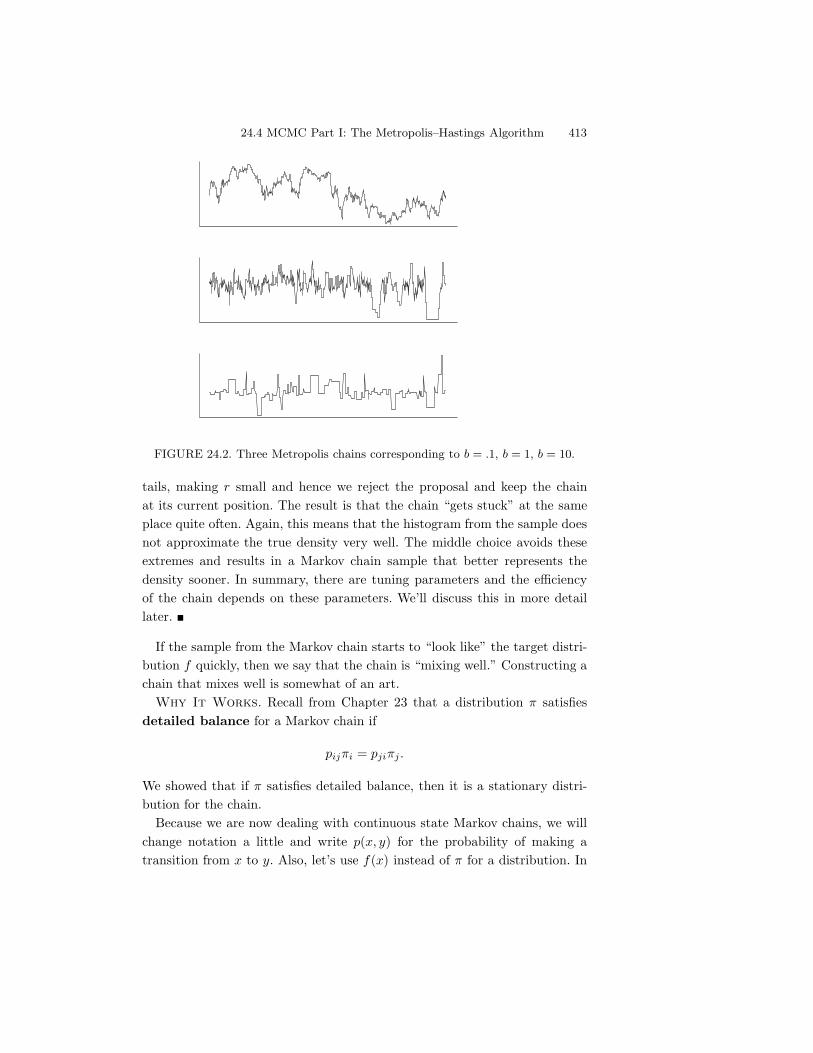
24.4 MCMC Part I: The Metropolis–Hastings Algorithm 413
FIGURE 24.2. Three Metropolis chains corresponding to b = .1, b = 1, b = 10.
tails, making r small and hence we reject the proposal and keep the chainat its current position. The result is that the chain “gets stuck” at the sameplace quite often. Again, this means that the histogram from the sample doesnot approximate the true density very well. The middle choice avoids theseextremes and results in a Markov chain sample that better represents thedensity sooner. In summary, there are tuning parameters and the e#ciencyof the chain depends on these parameters. We’ll discuss this in more detaillater. !
If the sample from the Markov chain starts to “look like” the target distri-bution f quickly, then we say that the chain is “mixing well.” Constructing achain that mixes well is somewhat of an art.
Why It Works. Recall from Chapter 23 that a distribution & satisfiesdetailed balance for a Markov chain if
pij&i = pji&j .
We showed that if & satisfies detailed balance, then it is a stationary distri-bution for the chain.
Because we are now dealing with continuous state Markov chains, we willchange notation a little and write p(x, y) for the probability of making atransition from x to y. Also, let’s use f(x) instead of & for a distribution. In
414 24. Simulation Methods
this new notation, f is a stationary distribution if f(x) =8
f(y)p(y, x)dy anddetailed balance holds for f if
f(x)p(x, y) = f(y)p(y, x). (24.7)
Detailed balance implies that f is a stationary distribution since, if detailedbalance holds, then
9f(y)p(y, x)dy =
9f(x)p(x, y)dy = f(x)
9p(x, y)dy = f(x)
which shows that f(x) =8
f(y)p(y, x)dy as required. Our goal is to show thatf satisfies detailed balance which will imply that f is a stationary distributionfor the chain.
Consider two points x and y. Either
f(x)q(y|x) < f(y)q(x|y) or f(x)q(y|x) > f(y)q(x|y).
We will ignore ties (which occur with probability zero for continuous distribu-tions). Without loss of generality, assume that f(x)q(y|x) > f(y)q(x|y). Thisimplies that
r(x, y) =f(y)f(x)
q(x|y)q(y|x)
and that r(y, x) = 1. Now p(x, y) is the probability of jumping from x to y.This requires two things: (i) the proposal distribution must generate y, and(ii) you must accept y. Thus,
p(x, y) = q(y|x)r(x, y) = q(y|x)f(y)f(x)
q(x|y)q(y|x)
=f(y)f(x)
q(x|y).
Therefore,
f(x)p(x, y) = f(y)q(x|y). (24.8)
On the other hand, p(y, x) is the probability of jumping from y to x. Thisrequires two things: (i) the proposal distribution must generate x, and (ii) youmust accept x. This occurs with probability p(y, x) = q(x|y)r(y, x) = q(x|y).Hence,
f(y)p(y, x) = f(y)q(x|y). (24.9)
Comparing (24.8) and (24.9), we see that we have shown that detailed balanceholds.
24.5 MCMC Part II: Di"erent Flavors 415
24.5 MCMC Part II: Di!erent Flavors
There are di!erent types of MCMC algorithm. Here we will consider a few ofthe most popular versions.
Random-Walk-Metropolis–Hastings. In the previous section we con-sidered drawing a proposal Y of the form
Y = Xi + -i
where -i comes from some distribution with density g. In other words, q(y|x) =g(y " x). We saw that in this case,
r(x, y) = min'
1,f(y)f(x)
2.
This is called a random-walk-Metropolis–Hastings method. The reasonfor the name is that, if we did not do the accept–reject step, we would besimulating a random walk. The most common choice for g is a N(0, b2). Thehard part is choosing b so that the chain mixes well. A good rule of thumb is:choose b so that you accept the proposals about 50 percent of the time.
Warning! This method doesn’t make sense unless X takes values on thewhole real line. If X is restricted to some interval then it is best to transformX . For example, if X $ (0,#) then you might take Y = log X and thensimulate the distribution for Y instead of X .
Independence-Metropolis–Hastings. This is an importance-samplingversion of MCMC. We draw the proposal from a fixed distribution g. Gen-erally, g is chosen to be an approximation to f . The acceptance probabilitybecomes
r(x, y) = min'
1,f(y)f(x)
g(x)g(y)
2.
Gibbs Sampling. The two previous methods can be easily adapted, inprinciple, to work in higher dimensions. In practice, tuning the chains to makethem mix well is hard. Gibbs sampling is a way to turn a high-dimensionalproblem into several one-dimensional problems.
Here’s how it works for a bivariate problem. Suppose that (X, Y ) has den-sity fX,Y (x, y). First, suppose that it is possible to simulate from the condi-tional distributions fX|Y (x|y) and fY |X(y|x). Let (X0, Y0) be starting values.Assume we have drawn (X0, Y0), . . . , (Xn, Yn). Then the Gibbs sampling al-gorithm for getting (Xn+1, Yn+1) is:
416 24. Simulation Methods
Gibbs Sampling
Xn+1 ! fX|Y (x|Yn)
Yn+1 ! fY |X(y|Xn+1)
repeat
This generalizes in the obvious way to higher dimensions.
24.11 Example (Normal Hierarchical Model). Gibbs sampling is very usefulfor a class of models called hierarchical models. Here is a simple case.Suppose we draw a sample of k cities. From each city we draw ni people andobserve how many people Yi have a disease. Thus, Yi ! Binomial(ni, pi). Weare allowing for di!erent disease rates in di!erent cities. We can also think ofthe p&is as random draws from some distribution F . We can write this modelin the following way:
Pi ! F
Yi|Pi = pi ! Binomial(ni, pi).
We are interested in estimating the p&is and the overall disease rate8
p dF (p).To proceed, it will simplify matters if we make some transformations that
allow us to use some Normal approximations. Let 1pi = Yi/ni. Recall that1pi . N(pi, si) where si =
31pi(1" 1pi)/ni. Let ,i = log(pi/(1 " pi)) and
define Zi 0 1,i = log(1pi/(1" 1pi)). By the delta method,
1,i . N(,i,#2i )
where #2i = 1/(n1pi(1"1pi)). Experience shows that the Normal approximation
for , is more accurate than the Normal approximation for p so we shall workwith ,. We shall treat #i as known. Furthermore, we shall take the distributionof the ,&
is to be Normal. The hierarchical model is now
,i ! N(µ, 22)
Zi|,i ! N(,i,#2i ).
As yet another simplification we take 2 = 1. The unknown parameter are0 = (µ,,1, . . . ,,k). The likelihood function is
L(0) 3/
i
f(,i|µ)/
i
f(Zi|,)
3/
i
exp'"1
2(,i " µ)2
2exp'" 1
2#2i
(Zi " ,i)22
.
24.5 MCMC Part II: Di"erent Flavors 417
If we use the prior f(µ) 3 1 then the posterior is proportional to the likelihood.To use Gibbs sampling, we need to find the conditional distribution of eachparameter conditional on all the others. Let us begin by finding f(µ|rest)where “rest” refers to all the other variables. We can throw away any termsthat don’t involve µ. Thus,
f(µ|rest) 3/
i
exp'"1
2(,i " µ)2
2
3 exp'"k
2(µ" b)2
2
whereb =
1k
*
i
,i.
Hence we see that µ|rest ! N(b, 1/k). Next we will find f(,|rest). Again, wecan throw away any terms not involving ,i leaving us with
f(,i|rest) 3 exp'"1
2(,i " µ)2
2exp'" 1
2#2i
(Zi " ,i)22
3 exp'" 1
2d2i
(,i " ei)22
where
ei =Zi
%2i
+ µ
1 + 1%2
i
and d2i =
11 + 1
%2i
and so ,i|rest ! N(ei, d2i ). The Gibbs sampling algorithm then involves iter-
ating the following steps N times:
draw µ ! N(b, v2)
draw ,1 ! N(e1, d21)
......
draw ,k ! N(ek, d2k).
It is understood that at each step, the most recently drawn version of eachvariable is used.
We generated a numerical example with k = 20 cities and n = 20 peoplefrom each city. After running the chain, we can convert each ,i back into pi
by way of pi = e+i/(1 + e+i). The raw proportions are shown in Figure 24.4.Figure 24.3 shows “trace plots” of the Markov chain for p1 and µ. Figure24.4 shows the posterior for µ based on the simulated values. The second
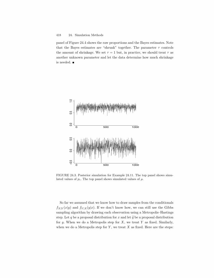
418 24. Simulation Methods
panel of Figure 24.4 shows the raw proportions and the Bayes estimates. Notethat the Bayes estimates are “shrunk” together. The parameter 2 controlsthe amount of shrinkage. We set 2 = 1 but, in practice, we should treat 2 asanother unknown parameter and let the data determine how much shrinkageis needed. !
0 500 1000
0.00.5
1.0
0 500 1000!0.5
0.00.5
FIGURE 24.3. Posterior simulation for Example 24.11. The top panel shows simu-lated values of p1. The top panel shows simulated values of µ.
So far we assumed that we know how to draw samples from the conditionalsfX|Y (x|y) and fY |X(y|x). If we don’t know how, we can still use the Gibbssampling algorithm by drawing each observation using a Metropolis–Hastingsstep. Let q be a proposal distribution for x and let cq be a proposal distributionfor y. When we do a Metropolis step for X , we treat Y as fixed. Similarly,when we do a Metropolis step for Y , we treat X as fixed. Here are the steps:
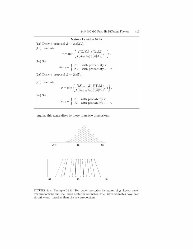
24.5 MCMC Part II: Di"erent Flavors 419
Metropolis within Gibbs
(1a) Draw a proposal Z ! q(z|Xn).(1b) Evaluate
r = min'
f(Z, Yn)f(Xn, Yn)
q(Xn|Z)q(Z|Xn)
, 12
.
(1c) Set
Xn+1 ='
Z with probability rXn with probability 1" r.
(2a) Draw a proposal Z ! cq(z|Yn).
(2b) Evaluate
r = min'
f(Xn+1, Z)f(Xn+1, Yn)
cq(Yn|Z)cq(Z|Yn)
, 12
.
(2c) Set
Yn+1 ='
Z with probability rYn with probability 1" r.
Again, this generalizes to more than two dimensions.
!0.6 0.0 0.6
0.0 0.5 1.0
FIGURE 24.4. Example 24.11. Top panel: posterior histogram of µ. Lower panel:raw proportions and the Bayes posterior estimates. The Bayes estimates have beenshrunk closer together than the raw proportions.
420 24. Simulation Methods
24.6 Bibliographic Remarks
MCMC methods go back to the e!ort to build the atomic bomb in World WarII. They were used in various places after that, especially in spatial statistics.There was a new surge of interest in the 1990s that still continues. My mainreference for this chapter was Robert and Casella (1999). See also Gelmanet al. (1995) and Gilks et al. (1998).
24.7 Exercises
1. Let
I =9 2
1
e$x2/2
/2&
dx.
(a) Estimate I using the basic Monte Carlo method. Use N = 100, 000.Also, find the estimated standard error.
(b) Find an (analytical) expression for the standard error of your esti-mate in (a). Compare to the estimated standard error.
(c) Estimate I using importance sampling. Take g to be N(1.5, v2) withv = .1, v = 1 and v = 10. Compute the (true) standard errors in eachcase. Also, plot a histogram of the values you are averaging to see ifthere are any extreme values.
(d) Find the optimal importance sampling function g*. What is thestandard error using g*?
2. Here is a way to use importance sampling to estimate a marginal density.Let fX,Y (x, y) be a bivariate density and let (X1, X2), . . . , (XN , YN ) !fX,Y .
(a) Let w(x) be an arbitrary probability density function. Let
1fX(x) =1N
N*
i=1
fX,Y (x, Yi)w(Xi)fX,Y (Xi, Yi)
.
Show that, for each x,1fX(x) p) fX(x).
Find an expression for the variance of this estimator.
(b) Let Y ! N(0, 1) and X |Y = y ! N(y, 1 + y2). Use the method in(a) to estimate fX(x).
24.7 Exercises 421
3. Here is a method called accept–reject sampling for drawing observa-tions from a distribution.
(a) Suppose that f is some probability density function. Let g be anyother density and suppose that f(x) , Mg(x) for all x, where M is aknown constant. Consider the following algorithm:
(step 1): Draw X ! g and U ! Unif(0, 1);
(step 2): If U , f(X)/(Mg(X)) set Y = X , otherwise go back to step1. (Keep repeating until you finally get an observation.)
Show that the distribution of Y is f .
(b) Let f be a standard Normal density and let g(x) = 1/(1 + x2) bethe Cauchy density. Apply the method in (a) to draw 1,000 observationsfrom the Normal distribution. Draw a histogram of the sample to verifythat the sample appears to be Normal.
4. A random variable Z has a inverse Gaussian distribution if it hasdensity
f(z) 3 z$3/2 exp'"01z "
02z
+ 230102 + log
+3202,2
, z > 0
where 01 > 0 and 02 > 0 are parameters. It can be shown that
E(Z) =U0201
and E-
1Z
.=U0102
+1
202.
(a) Let 01 = 1.5 and 02 = 2. Draw a sample of size 1,000 using theindependence-Metropolis–Hastings method. Use a Gamma distributionas the proposal density. To assess the accuracy, compare the mean of Z
and 1/Z from the sample to the theoretical means Try di!erent Gammadistributions to see if you can get an accurate sample.
(b) Draw a sample of size 1,000 using the random-walk-Metropolis–Hastings method. Since z > 0 we cannot just use a Normal density.One strategy is this. Let W = log Z. Find the density of W . Use therandom-walk-Metropolis–Hastings method to get a sample W1, . . . , WN
and let Zi = eWi . Assess the accuracy of the simulation as in part (a).
5. Get the heart disease data from the book web site. Consider a Bayesiananalysis of the logistic regression model
P(Y = 1|X = x) =e"0+
0kj=1 "jxj
1 + e"0+0k
j=1 "jxj.

422 24. Simulation Methods
Use the flat prior f((0, . . . ,(k) 3 1. Use the Gibbs–Metropolis algorithmto draw a sample of size 10,000 from the posterior f((0,(1|data). Plothistograms of the posteriors for the (j ’s. Get the posterior mean and a95 percent posterior interval for each (j .
(b) Compare your analysis to a frequentist approach using maximumlikelihood.

This is page 423Printer: Opaque this
Bibliography
Agresti, A. (1990). Categorical Data Analysis. Wiley.
Akaike, H. (1973). Information theory and an extension of the maximumlikelihood principle. Second International Symposium on Information The-ory 267–281.
Anderson, T. W. (1984). An Introduction to Multivariate Statistical Anal-ysis (Second Edition). Wiley.
Barron, A., Schervish, M. J. and Wasserman, L. (1999). The consis-tency of posterior distributions in nonparametric problems. The Annals ofStatistics 27 536–561.
Beecher, H. (1959). Measurement of Subjective Responses. Oxford Univer-sity Press.
Benjamini, Y. and Hochberg, Y. (1995). Controlling the false discoveryrate: A practical and powerful approach to multiple testing. Journal of theRoyal Statistical Society, Series B, Methodological 57 289–300.
Beran, R. (2000). REACT scatterplot smoothers: Supere#ciency throughbasis economy. Journal of the American Statistical Association 95 155–171.
Beran, R. and Dumbgen, L. (1998). Modulation of estimators and confi-dence sets. The Annals of Statistics 26 1826–1856.
424 Bibliography
Berger, J. and Wolpert, R. (1984). The Likelihood Principle. Instituteof Mathematical Statistics.
Berger, J. O. (1985). Statistical Decision Theory and Bayesian Analysis(Second Edition). Springer-Verlag.
Berger, J. O. and Delampady, M. (1987). Testing precise hypotheses (c/r:P335-352). Statistical Science 2 317–335.
Berliner, L. M. (1983). Improving on inadmissible estimators in the controlproblem. The Annals of Statistics 11 814–826.
Bickel, P. J. and Doksum, K. A. (2000). Mathematical Statistics: BasicIdeas and Selected Topics, Vol. I (Second Edition). Prentice Hall.
Billingsley, P. (1979). Probability and Measure. Wiley.
Bishop, Y. M. M., Fienberg, S. E. and Holland, P. W. (1975). DiscreteMultivariate Analyses: Theory and Practice. MIT Press.
Breiman, L. (1992). Probability. Society for Industrial and Applied Mathe-matics.
Brinegar, C. S. (1963). Mark Twain and the Quintus Curtius Snodgrassletters: A statistical test of authorship. Journal of the American StatisticalAssociation 58 85–96.
Carlin, B. P. and Louis, T. A. (1996). Bayes and Empirical Bayes Methodsfor Data Analysis. Chapman & Hall.
Casella, G. and Berger, R. L. (2002). Statistical Inference. DuxburyPress.
Chaudhuri, P. and Marron, J. S. (1999). Sizer for exploration of structuresin curves. Journal of the American Statistical Association 94 807–823.
Cox, D. and Lewis, P. (1966). The Statistical Analysis of Series of Events.Chapman & Hall.
Cox, D. D. (1993). An analysis of Bayesian inference for nonparametricregression. The Annals of Statistics 21 903–923.
Cox, D. R. and Hinkley, D. V. (2000). Theoretical statistics. Chapman &Hall.
425
Davison, A. C. and Hinkley, D. V. (1997). Bootstrap Methods and TheirApplication. Cambridge University Press.
DeGroot, M. and Schervish, M. (2002). Probability and Statistics (ThirdEdition). Addison-Wesley.
Devroye, L., Gyorfi, L. and Lugosi, G. (1996). A Probabilistic Theoryof Pattern Recognition. Springer-Verlag.
Diaconis, P. and Freedman, D. (1986). On inconsistent Bayes estimatesof location. The Annals of Statistics 14 68–87.
Dobson, A. J. (2001). An introduction to generalized linear models. Chap-man & Hall.
Donoho, D. L. and Johnstone, I. M. (1994). Ideal spatial adaptation bywavelet shrinkage. Biometrika 81 425–455.
Donoho, D. L. and Johnstone, I. M. (1995). Adapting to unknownsmoothness via wavelet shrinkage. Journal of the American Statistical As-sociation 90 1200–1224.
Donoho, D. L. and Johnstone, I. M. (1998). Minimax estimation viawavelet shrinkage. The Annals of Statistics 26 879–921.
Donoho, D. L., Johnstone, I. M., Kerkyacharian, G. and Picard, D.
(1995). Wavelet shrinkage: Asymptopia? (Disc: p 337–369). Journal of theRoyal Statistical Society, Series B, Methodological 57 301–337.
Dunsmore, I., Daly, F. et al. (1987). M345 Statistical Methods, Unit 9:Categorical Data. The Open University.
Edwards, D. (1995). Introduction to graphical modelling. Springer-Verlag.
Efromovich, S. (1999). Nonparametric Curve Estimation: Methods, Theoryand Applications. Springer-Verlag.
Efron, B. (1979). Bootstrap methods: Another look at the jackknife. TheAnnals of Statistics 7 1–26.
Efron, B., Tibshirani, R., Storey, J. D. and Tusher, V. (2001). Em-pirical Bayes analysis of a microarray experiment. Journal of the AmericanStatistical Association 96 1151–1160.
426 Bibliography
Efron, B. and Tibshirani, R. J. (1993). An Introduction to the Bootstrap.Chapman & Hall.
Ferguson, T. (1967). Mathematical Statistics : a Decision Theoretic Ap-proach. Academic Press.
Fisher, R. (1921). On the probable error of a coe#cient of correlation de-duced from a small sample. Metron 1 1–32.
Freedman, D. (1999). Wald lecture: On the Bernstein-von Mises theoremwith infinite-dimensional parameters. The Annals of Statistics 27 1119–1141.
Friedman, J. H. (1997). On bias, variance, 0/1-loss, and the curse-of-dimensionality. Data Mining and Knowledge Discovery 1 55–77.
Gelman, A., Carlin, J. B., Stern, H. S. and Rubin, D. B. (1995).Bayesian Data Analysis. Chapman & Hall.
Ghosal, S., Ghosh, J. K. and Van Der Vaart, A. W. (2000). Conver-gence rates of posterior distributions. The Annals of Statistics 28 500–531.
Gilks, W. R., Richardson, S. and Spiegelhalter, D. J. (1998). MarkovChain Monte Carlo in Practice. Chapman & Hall.
Grimmett, G. and Stirzaker, D. (1982). Probability and Random Pro-cesses. Oxford University Press.
Guttorp, P. (1995). Stochastic Modeling of Scientific Data. Chapman &Hall.
Hall, P. (1992). The Bootstrap and Edgeworth Expansion. Springer-Verlag.
Halverson, N., Leitch, E., Pryke, C., Kovac, J., Carlstrom, J.,Holzapfel, W., Dragovan, M., Cartwright, J., Mason, B., Padin,
S., Pearson, T., Shepherd, M. and Readhead, A. (2002). DASI firstresults: A measurement of the cosmic microwave background angular powerspectrum. Astrophysics Journal 568 38–45.
Hardle, W. (1990). Applied nonparametric regression. Cambridge Univer-sity Press.
Hardle, W., Kerkyacharian, G., Picard, D. and Tsybakov, A. (1998).Wavelets, Approximation, and Statistical Applications. Springer-Verlag.
427
Hastie, T., Tibshirani, R. and Friedman, J. H. (2001). The Elementsof Statistical Learning: Data Mining, Inference, and Prediction. Springer-Verlag.
Herbich, R. (2002). Learning Kernel Classifiers: Theory and Algorithms.MIT Press.
Johnson, R. A. and Wichern, D. W. (1982). Applied Multivariate Statis-tical Analysis. Prentice-Hall.
Johnson, S. and Johnson, R. (1972). New England Journal of Medicine287 1122–1125.
Jordan, M. (2004). Graphical models. In Preparation.
Karr, A. (1993). Probability. Springer-Verlag.
Kass, R. E. and Raftery, A. E. (1995). Bayes factors. Journal of theAmerican Statistical Association 90 773–795.
Kass, R. E. and Wasserman, L. (1996). The selection of prior distributionsby formal rules (corr: 1998 v93 p 412). Journal of the American StatisticalAssociation 91 1343–1370.
Larsen, R. J. and Marx, M. L. (1986). An Introduction to MathematicalStatistics and Its Applications (Second Edition). Prentice Hall.
Lauritzen, S. L. (1996). Graphical Models. Oxford University Press.
Lee, A. T. et al. (2001). A high spatial resolution analysis of the maxima-1cosmic microwave background anisotropy data. Astrophys. J. 561 L1–L6.
Lee, P. M. (1997). Bayesian Statistics: An Introduction. Edward Arnold.
Lehmann, E. L. (1986). Testing Statistical Hypotheses (Second Edition).Wiley.
Lehmann, E. L. and Casella, G. (1998). Theory of Point Estimation.Springer-Verlag.
Loader, C. (1999). Local regression and likelihood. Springer-Verlag.
Marron, J. S. and Wand, M. P. (1992). Exact mean integrated squarederror. The Annals of Statistics 20 712–736.
428 Bibliography
Morrison, A., Black, M., Lowe, C., Macmahon, B. and Yusa, S.
(1973). Some international di!erences in histology and survival in breastcancer. International Journal of Cancer 11 261–267.
Netterfield, C. B. et al. (2002). A measurement by boomerang of mul-tiple peaks in the angular power spectrum of the cosmic microwave back-ground. Astrophys. J. 571 604–614.
Ogden, R. T. (1997). Essential Wavelets for Statistical Applications andData Analysis. Birkhauser.
Pearl, J. (2000). Casuality: models, reasoning, and inference. CambridgeUniversity Press.
Phillips, D. and King, E. (1988). Death takes a holiday: Mortality sur-rounding major social occasions. Lancet 2 728–732.
Phillips, D. and Smith, D. (1990). Postponement of death until symbol-ically meaningful occasions. Journal of the American Medical Association263 1947–1961.
Quenouille, M. (1949). Approximate tests of correlation in time series.Journal of the Royal Statistical Society B 11 18–84.
Rice, J. A. (1995). Mathematical Statistics and Data Analysis (Second Edi-tion). Duxbury Press.
Robert, C. P. (1994). The Bayesian Choice: A Decision-theoretic Motiva-tion. Springer-Verlag.
Robert, C. P. and Casella, G. (1999). Monte Carlo Statistical Methods.Springer-Verlag.
Robins, J., Scheines, R., Spirtes, P. and Wasserman, L. (2003). Uniformconvergence in causal inference. Biometrika (to appear).
Robins, J. M. and Ritov, Y. (1997). Toward a curse of dimensionality ap-propriate (CODA) asymptotic theory for semi-parametric models. Statisticsin Medicine 16 285–319.
Rosenbaum, P. (2002). Observational Studies. Springer-Verlag.
Ross, S. (2002). Probability Models for Computer Science. Academic Press.
429
Rousseauw, J., du Plessis, J., Benade, A., Jordaan, P., Kotze, J.,Jooste, P. and Ferreira, J. (1983). Coronary risk factor screening inthree rural communities. South African Medical Journal 64 430–436.
Schervish, M. J. (1995). Theory of Statistics. Springer-Verlag.
Scholkopf, B. and Smola, A. (2002). Learning with Kernels: SupportVector Machines, Regularization, Optimization, and Beyond. MIT Press.
Schwarz, G. (1978). Estimating the dimension of a model. The Annals ofStatistics 6 461–464.
Scott, D., Gotto, A., Cole, J. and Gorry, G. (1978). Plasma lipids ascollateral risk factors in coronary artery disease: a study of 371 males withchest pain. Journal of Chronic Diseases 31 337–345.
Scott, D. W. (1992). Multivariate Density Estimation: Theory, Practice,and Visualization. Wiley.
Shao, J. and Tu, D. (1995). The Jackknife and Bootstrap (German).Springer-Verlag.
Shen, X. and Wasserman, L. (2001). Rates of convergence of posteriordistributions. The Annals of Statistics 29 687–714.
Shorack, G. R. and Wellner, J. A. (1986). Empirical Processes WithApplications to Statistics. Wiley.
Silverman, B. W. (1986). Density Estimation for Statistics and Data Anal-ysis. Chapman & Hall.
Spirtes, P., Glymour, C. N. and Scheines, R. (2000). Causation, predic-tion, and search. MIT Press.
Taylor, H. M. and Karlin, S. (1994). An Introduction to Stochastic Mod-eling. Academic Press.
van der Laan, M. and Robins, J. (2003). Unified Methods for CensoredLongitudinal Data and Causality. Springer Verlag.
van der Vaart, A. W. (1998). Asymptotic Statistics. Cambridge UniversityPress.
van der Vaart, A. W. and Wellner, J. A. (1996). Weak Convergenceand Empirical Processes: With Applications to Statistics. Springer-Verlag.
430 Bibliography
Vapnik, V. N. (1998). Statistical Learning Theory. Wiley.
Weisberg, S. (1985). Applied Linear Regression. Wiley.
Whittaker, J. (1990). Graphical Models in Applied Multivariate Statistics.Wiley.
Wright, S. (1934). The method of path coe#cients. The Annals of Mathe-matical Statistics 5 161–215.
Zhao, L. H. (2000). Bayesian aspects of some nonparametric problems. TheAnnals of Statistics 28 532–552.
Zheng, X. and Loh, W.-Y. (1995). Consistent variable selection in linearmodels. Journal of the American Statistical Association 90 151–156.
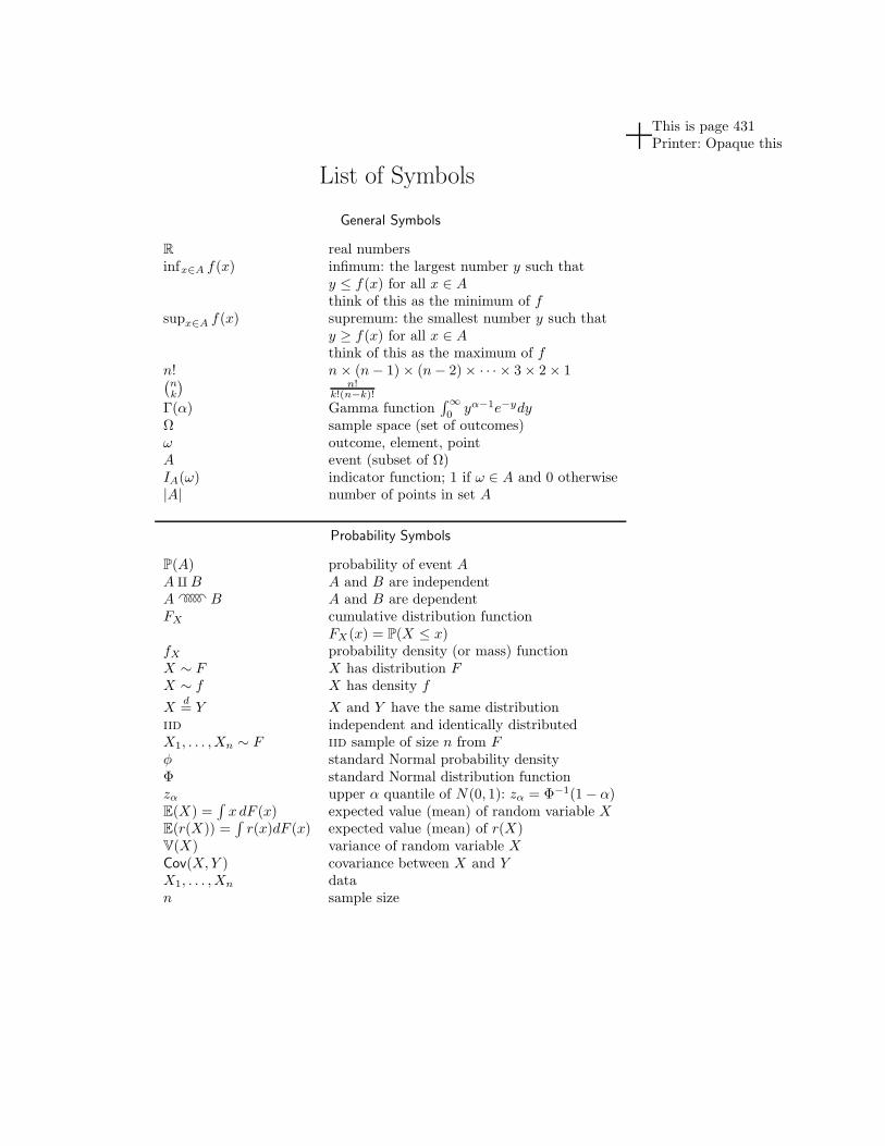
This is page 431Printer: Opaque this
List of Symbols
General Symbols
R real numbersinfx#A f(x) infimum: the largest number y such that
y , f(x) for all x $ Athink of this as the minimum of f
supx#A f(x) supremum: the smallest number y such thaty * f(x) for all x $ Athink of this as the maximum of f
n! n- (n" 1)- (n" 2)- · · ·- 3- 2- 1;nk
<n!
k!(n$k)!
&()) Gamma function8!0 y#$1e$ydy
$ sample space (set of outcomes)" outcome, element, pointA event (subset of $)IA(") indicator function; 1 if " $ A and 0 otherwise|A| number of points in set A
Probability Symbols
P(A) probability of event AA ! B A and B are independentA !""""# B A and B are dependentFX cumulative distribution function
FX(x) = P(X , x)fX probability density (or mass) functionX ! F X has distribution FX ! f X has density f
Xd= Y X and Y have the same distribution
iid independent and identically distributedX1, . . . , Xn ! F iid sample of size n from F' standard Normal probability density% standard Normal distribution functionz# upper ) quantile of N(0, 1): z# = %$1(1" ))E(X) =
8xdF (x) expected value (mean) of random variable X
E(r(X)) =8
r(x)dF (x) expected value (mean) of r(X)V(X) variance of random variable XCov(X, Y ) covariance between X and YX1, . . . , Xn datan sample size
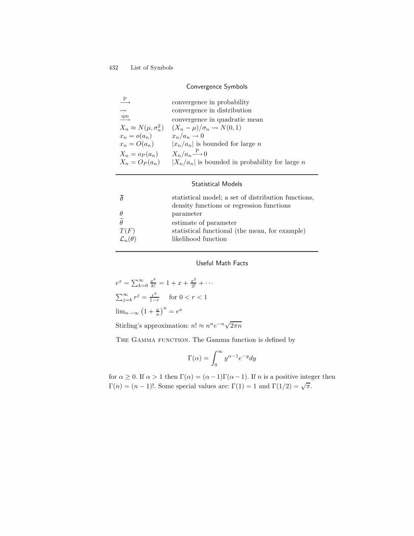
432 List of Symbols
Convergence Symbols
P") convergence in probability! convergence in distributionqm") convergence in quadratic meanXn . N(µ,#2
n) (Xn " µ)/#n ! N(0, 1)xn = o(an) xn/an ) 0xn = O(an) |xn/an| is bounded for large n
Xn = oP (an) Xn/anP") 0
Xn = OP (an) |Xn/an| is bounded in probability for large n
Statistical Models
F statistical model; a set of distribution functions,density functions or regression functions
0 parameter10 estimate of parameterT (F ) statistical functional (the mean, for example)Ln(0) likelihood function
Useful Math Facts
ex =0!
k=0xk
k! = 1 + x + x2
2! + · · ·0!
j=k rj = rk
1$r for 0 < r < 1
limn"!;1 + a
n
<n = ea
Stirling’s approximation: n! . nne$n/
2&n
The Gamma function. The Gamma function is defined by
&()) =9 !
0y#$1e$ydy
for ) * 0. If ) > 1 then &()) = ()"1)&()"1). If n is a positive integer then&(n) = (n" 1)!. Some special values are: &(1) = 1 and &(1/2) =
/&.
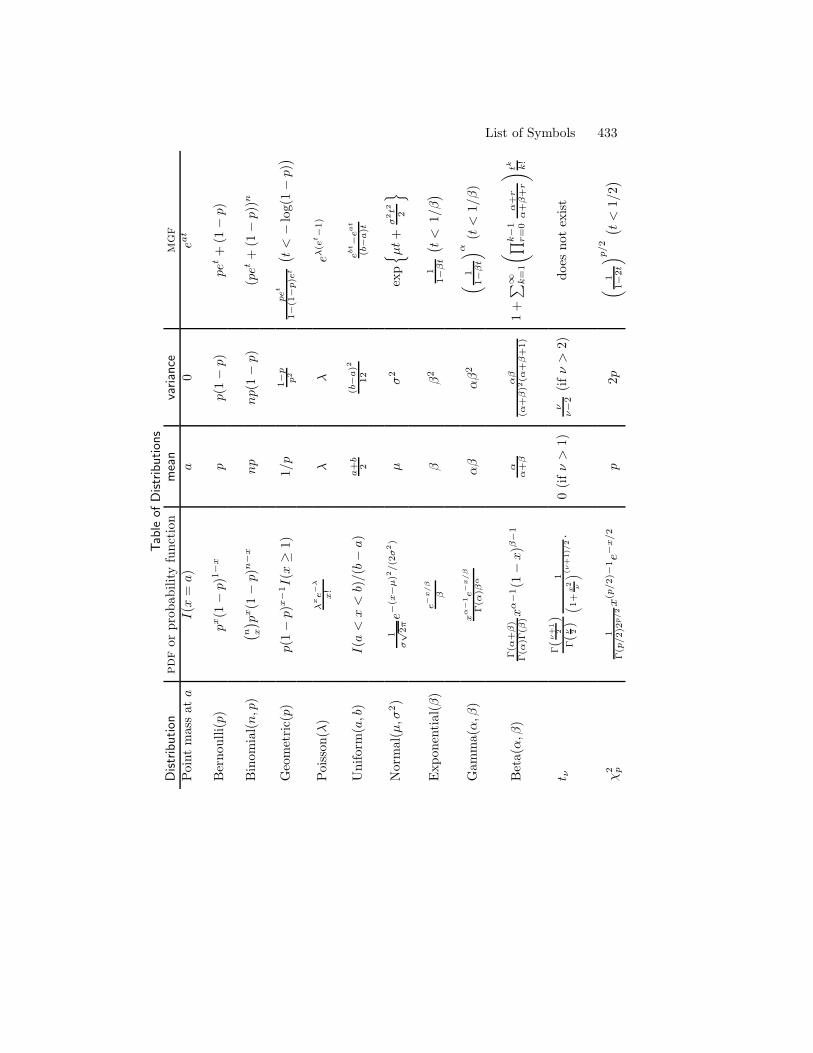
Tab
leof
Distr
ibut
ions
List of Symbols 433
Distr
ibut
ion
orpr
obab
ility
func
tion
mea
nva
rian
cemgf
Poi
ntm
ass
ata
I(x
=a)
a0
eat
Ber
noul
li(p)
px(1"
p)1$
xp
p(1"
p)pe
t+
(1"
p)
Bin
omia
l(n,p
); n x
< px(1"
p)n$
xnp
np(
1"
p)(p
et+
(1"
p))n
Geo
met
ric(
p)p(
1"
p)x$
1I(
x*
1)1/
p1$
pp2
pe
t
1$
(1$
p)e
t
; t<"
log(
1"
p)<
Poi
sson
(%)
!xe#
$
x!
%%
e!(e
t$
1)
Uni
form
(a,b
)I(
a<
x<
b)/(
b"
a)a+
b2
(b$
a)2
12
ebt$
ea
t
(b$
a)t
Nor
mal
(µ,#
2)
1%(
2-e$
(x$
µ)2
/(2%
2)
µ#
2ex
p! µ
t+%
2t2 2
"
Exp
onen
tial
(()
e#
x/
%
"(
(2
11$"
t
; t<
1/(<
Gam
ma(),(
)x
&#
1e#
x/
%
$(#
)"&
)(
)(
2+
11$"
t
, #(t
<1/()
Bet
a(),(
)$(#
+")
$(#
)$("
)x#$
1(1"
x)"
$1
##+"
#"
(#+")2
(#+"+
1)
1+0
! k=
1
-D
k$
1r=
0#+
r#+"+
r
.tk k!
t $$('
+1
2)
$(' 2
)1
+1+
x2 '
,('
+1)/
2.
0(if*
>1)
$$$
2(if*
>2)
does
not
exis
t
!2 p
1$(p
/2)2
p/2x
(p/2)$
1e$
x/2
p2p
+1
1$
2t
, p/2; t
<1/
2<
This is pagePrinter: Opaque this
Index
!2 distribution, 30
accept-reject sampling, 421accessible, 387actions, 193acyclic, 266additive regression, 323adjacent, 281adjusted treatment e!ect, 259admissibility
Bayes rules, 202admissible, 202AIC (Akaike Information Criterion),
220Aliens, 271alternative hypothesis, 95, 149ancestor, 265aperiodic, 390arcs, 281associated, 239association, 253
association is not causation, 16.1,253
assume, 8asymptotic Normality, 128asymptotic theory, 71asymptotically Normal, 92, 126asymptotically optimal, 126asymptotically uniformly integrable,
81average causal e!ect, 252average treatment e!ect, 252Axiom 1, 5Axiom 2, 5Axiom 3, 5axioms of probability, 5
backfitting, 324bagging, 375bandwidth, 313Bayes classification rule, 351Bayes Estimators, 197Bayes risk, 195
Index
Bayes rules, 197admissibility, 202
Bayes’ Theorem, 12, 1.17, 12Bayesian inference, 89, 175
strengths and weaknesses, 185Bayesian network, 263Bayesian philosophy, 175Bayesian testing, 184Benjamini and Hochberg, 10.26, 167Benjamini-Hochberg (BH) method,
167Bernoulli distribution, 26, 29Beta distribution, 30bias-variance tradeo!, 305Bibliographic Remarks, 13Binomial distribution, 26bins, 303, 306binwidth, 306bivariate distribution, 31Bonferroni method, 166boosting, 375bootstrap, 107
parametric, 134Bootstrap Confidence Intervals, 110bootstrap percentile interval, 111bootstrap pivotal confidence, 111Bootstrap variance estimation, 109branching process, 398
candidate, 411Cauchy distribution, 30Cauchy-Schwartz inequality, 4.8, 66causal odds ratio, 252causal regression function, 256causal relative risk, 253Central Limit Theorem (CLT), 5.8,
77Chapman-Kolmogorov equations, 23.9,
385
Chebyshev’s inequality, 4.2, 64checking assumptions, 135child, 265classes, 387classification, 349classification rule, 349classification trees, 360classifier
assessing error rate, 362clique, 285closed, 388CLT, 77collider, 265comparing risk functions, 194complete, 281, 328composite hypothesis, 151Computer Experiment, 16, 17concave, 66conditional causal e!ect, 255conditional distribution, 36conditional expectation, 54conditional independence, 264
minimal, 287conditional likelihood, 213Conditional Probability, 10conditional probability, 10, 10conditional probability density func-
tion, 37conditional probability mass func-
tion, 36conditioning by intervention, 274conditioning by observation, 274confidence band, 99confidence bands, 323confidence interval, 65, 92confidence set, 92confounding variables, 257conjugate, 179
Index
consistency relationship, 252consistent, 90, 126continuity of probabilities, 1.8, 7continuous, 23converges in distribution, 72converges in probability, 72convex, 66correlation, 52
confidence interval, 234cosine basis, 329counterfactual, 251, 252counting process, 395covariance, 52covariance matrix, 232covariate, 209coverage, 92critical value, 150cross-validation, 363cross-validation estimator of risk,
310cumulative distribution function, 20curse of dimensionality, 319curve estimation, 89, 303
d-connected, 270d-separated, 270DAG, 266data mining, viidecision rule, 193decision theory, 193decomposition theorem, 23.17, 389delta method, 5.13, 79, 131density estimation, 312
kernel approach, 312orthogonal function approach,
331dependent, 34, 239dependent variable, 89derive, 8
descendant, 265detail coe#cients, 342detailed balance, 391, 413deviance, 299directed acyclic graph, 266directed graph, 264directed path, 265discrete, 22discrete uniform distribution, 26discrete wavelet transform (DWT),
344discriminant function, 354discrimination, 349disjoint, 5distribution
!2, 30Bernoulli, 26, 29Beta, 30Binomial, 26Cauchy, 30conditional, 36discrete uniform, 26Gaussian, 28Geometric, 26Multinomial, 39multivariate Normal, 39Normal, 28point mass, 26Poisson, 27t, 30Uniform, 27
Dvoretzky-Kiefer-Wolfowitz (DKW)inequality, 7.5, 98
edges, 281e#cient, 126, 131elements, 3EM algorithm, 144empirical distribution function, 97
Index
empirical error rate, 351empirical probability measure, 367empirical risk minimization, 352, 365Epanechnikov kernel, 312equal in distribution, 25equivariant, 126ergodic, 390Events, 3events, 3evidence, 157Exercises, 13expectation, 47
conditional, 54expected value, 47exponential families, 140
faithful, 270false discovery proportion, 166false discovery rate, 166FDP, 166FDR, 166feature, 89, 209first moment, 47first quartile, 25Fisher information, 128Fisher information matrix, 133Fisher linear discriminant function,
356fitted line, 210fitted values, 210frequentist (or classical), 175frequentist inference, 89
Gamma function, 29Gaussian classifier, 353Gaussian distribution, 28Geometric distribution, 26Gibbs sampling, 416Gini index, 361
Glivenko-Cantelli theorem, 7.4, 98goodness-of-fit tests, 168graphical, 294graphical log-linear models, 294
Haar father wavelet, 340Haar scaling function, 340Haar wavelet regression, 343hierarchical log-linear model, 296hierarchical model, 56hierarchical models, 416histogram, 303, 305histogram estimator, 306Hoe!ding’s inequality, 4.4, 64, 365homogeneous, 384homogeneous Poisson process, 396Horwitz-Thompson, 188hypothesis testing, 94
identifiable, 126importance sampling, 408impurity, 360inadmissible, 202independent, 8, 8, 34Independent Events, 8independent random variables, 34independent variable, 89index set, 381indicator function, 5inequalities, 63inner product, 327integrated squared error (ISE), 304intensity function, 395interarrival times, 396intervene, 273intervention, 273Introduction, 3invariant, 390inverse Gaussian distribution, 421
Index
irreducible, 388iterated expectations, 3.24, 55
jackknife, 115James-Stein estimator, 204Je!reys-Lindley paradox, 192Jensen’s inequality, 4.9, 66joint mass function, 31
K-fold cross-validation, 364k-nearest-neighbors, 375kernel, 312kernel density estimator, 312, 313kernelization, 371Kolmogorov-Smirnov test, 245Kullback-Leibler distance, 126
Laplace transform, 56large sample theory, 71law of large numbers, 72law of total probability, 1.16, 12lazy, 3.6, 48least favorable prior, 198least squares estimates, 211leave-one-out cross-validation, 220leaves, 361Legendre polynomials, 329length, 327level, 150likelihood function, 122likelihood ratio statistic, 164likelihood ratio test, 164limit theory, 71limiting distribution, 391linear algebra notation, 231linear classifier, 353linearly separable, 369log odds ratio, 240log-likelihood function, 122
log-linear expansion, 292log-linear model, 286log-linear models, 291logistic regression, 223loss function, 193
machine learning, viiManalahobis distance, 353marginal Distribution, 33marginal distribution, 197Markov chain, 383, 383Markov condition, 267Markov equivalent, 271Markov’s inequality, 4.1, 63maximal clique, 285maximum likelihood, 122maximum likelihood estimates
computing, 142maximum likelihood estimator
consistent, 126maximum risk, 195mean, 47mean integrated squared error (MISE),
304mean recurrence time, 390mean squared error, 91measurable, 13, 43median, 25
bootstrap, 109Mercer’s theorem, 373method of moments estimator, 121Metropolis within Gibbs, 419Metropolis–Hastings algorithm, 411Mill’s inequality, 4.7, 65minimal conditional independence,
287minimal su#cient, 138minimax rule, 197, 198missing data, 187
Index
mixture of Normals, 143model generator, 297model selection, 218moment generating function, 56moments, 49monotone decreasing, 5monotone increasing, 5Monte Carlo integration, 404Monte Carlo integration method,
404Monty Hall, 14most powerful, 152mother Haar wavelet, 341MSE, 91Multinomial, 235Multinomial distribution, 39multiparameter models, 133multiple regression, 216multiple testing, 165multiresolution analysis, 341Multivariate central limit theorem,
5.12, 78Multivariate Delta Method, 5.15,
79multivariate Normal, 234multivariate Normal distribution, 39mutually exclusive, 5
Nadaraya-Watson kernel estimator,319
naive Bayes classifier, 359natural parameter, 141natural su#cient statistic, 140neural networks, 376Newton-Raphson, 143Neyman-Pearson, 10.30, 170nodes, 281non-collider, 265non-null, 390
nonparametric model, 88nonparametric regression, 319
kernel approach, 319orthogonal function approach,
337norm, 327normal, 327Normal distribution, 28Normal-based confidence interval,
6.16, 94normalizing constant, 177, 403not, 10nuisance parameter, 120nuisance parameters, 88null, 390null hypothesis, 94, 149
observational studies, 257odds ratio, 240olive statistics, ione-parameter exponential family,
140one-sided test, 151optimality, 130orthogonal, 327orthogonal functions, 327orthonormal, 328orthonormal basis, 328outcome, 89overfitting, 218
p-value, 156, 157pairwise Markov graph, 283parameter of interest, 120parameter space, 88parameters, 26parametric bootstrap, 134parametric model, 87parent, 265
Index
Parseval’s relation, 329partition, 5path, 281Pearson’s !2 test, 241period, 390periodic, 390permutation distribution, 162permutation test, 161permutation test:algorithm, 163perpendicular, 327persistent, 388pivot, 110plug-in estimator, 99point estimation, 90point mass distribution, 26pointwise asymptotic, 95Poisson distribution, 27Poisson process, 394, 395positive definite, 231posterior, 176
large sample properties, 181posterior risk, 197potential, 285potential outcomes, 251power function, 150precision matrix, 232predicted values, 210prediction, 89, 215prediction interval, 13.11, 215prediction risk, 219predictor, 89predictor variable, 209prior distribution, 176Probability, 5probability, 5probability distribution, 5, 5probability function, 22probability inequalities, 63
probability mass function, 22probability measure, 5, 5Probability on Finite Sample Spaces,
7proposal, 411
quadratic discriminant analysis (QDA),353
quantile function, 25quantiles, 102
random variable, 19independent, 34
random vector, 38, 232random walk, 59random-walk-Metropolis-Hastings,
415realizations, 3recurrence time, 390recurrent, 388regression, 89, 209, 335
nonparametric, 319regression function, 89, 209, 351regression through the origin, 226regressor, 89rejection region, 150relative risk, 248represents, 266residual sums of squares, 211residuals, 210response variable, 89, 209reweighted least squares, 224risk, 194, 304rule of the lazy statistician, 3.6, 48Rules of d-separation, 270
sample correlation, 102sample mean, 51sample outcomes, 3
Index
sample quantile, 102sample space, 3Sample Spaces and Events, 3sample variance, 51sampling distribution, 90saturated model, 298, 299scaling coe#cient, 342score function, 128se, 90shatter coe#cient, 367shattered, 367simple hypothesis, 151simple linear regression, 210Simpson’s paradox, 259simulation, 108, 180size, 150slack variables, 371Slutzky’s theorem, 75smoothing, 303smoothing parameter, 303Sobolev space, 88sojourn times, 396spatially inhomogeneous, 340standard deviation, 51standard error, 90standard Normal distribution, 28state space, 381stationary, 390statistic, 61, 107, 137statistical functional, 89, 99statistical model, 87Stein’s paradox, 204stochastic process, 381Stone’s theorem, 20.16, 316strong law of large numbers, 5.18,
81strongly inadmissible, 204subjectivism, 181
su#ciency, 137su#cient statistic, 137Summary of Terminology, 4supervised learning, 349support vector machines, 368support vectors, 370
t distribution, 30t-test, 170test statistic, 150third quartile, 25thresholding, 342training error, 219training error rate, 351training set, 363transformations of random variables,
41transient, 388true error rate, 351two-sided test, 151type I error, 150type II error, 150types of convergence, 72
unbiased, 90underfitting, 218undirected graph, 281uniform asymptotic, 95Uniform distribution, 27unshielded collider, 266
validation set, 363Vapnik-Chervonenkis, 366variance, 51
conditional, 55variance-covariance matrix, 53vertices, 281
waiting times, 396Wald test, 153

Index
wavelets, 340weak law of large numbers (WLLN),
5.6, 76
Zheng-Loh method, 222