A little bit of help with Maple - University of Wollongongweb/@i… · · 2015-06-05A little bit of help with Maple School of Mathematics and Applied Statistics ... The aim of this

A little bit of help with Maple

School of Mathematics and Applied StatisticsUniversity of Wollongong

2008

http://www.uow.edu.au/informatics/maths/

http://www.uow.edu.au/


Welcome!

The aim of this manual is to provide you with a little bit of help with Maple. Inside you willfind brief descriptions on a lot of useful commands and packages that are commonly neededwhen using Maple. Full worked examples are presented to show you how to use the Maplecommands, with different options given, where the aim is to teach you Maple by example –not by showing the full technical detail. If you want the full detail, you are encouraged tolook at the Maple Help menu.

To use this manual, a basic understanding of mathematics and how to use a computer isassumed. While this manual is based on Version 10.01 of Maple on the PC platform on Win-dows XP, most of it should be applicable to other versions, platforms and operating systems.

This handbook is built upon the original version of this handbook by Maureen Edwards andAlex Antic. Further information has been gained from the Help menu in Maple itself.

If you have any suggestions or comments, please email them to Grant Cox ([email protected]).

Table of contents : Index 1/81

Contents

1 Introduction 41.1 What is Maple? . . . . . . . . . . . . . . . . . . . . . . . . . . . . . . . . . . . 41.2 Getting started . . . . . . . . . . . . . . . . . . . . . . . . . . . . . . . . . . . 41.3 Operators . . . . . . . . . . . . . . . . . . . . . . . . . . . . . . . . . . . . . . 7

1.3.1 The Ditto Operator . . . . . . . . . . . . . . . . . . . . . . . . . . . . . 91.4 Assign and unassign . . . . . . . . . . . . . . . . . . . . . . . . . . . . . . . . 91.5 Special constants . . . . . . . . . . . . . . . . . . . . . . . . . . . . . . . . . . 111.6 Evaluation . . . . . . . . . . . . . . . . . . . . . . . . . . . . . . . . . . . . . . 11

1.6.1 Digits . . . . . . . . . . . . . . . . . . . . . . . . . . . . . . . . . . . . 131.6.2 The absolute value and the sign of a number . . . . . . . . . . . . . . . 13

1.7 Automatic simplifications . . . . . . . . . . . . . . . . . . . . . . . . . . . . . 151.8 Sets and lists . . . . . . . . . . . . . . . . . . . . . . . . . . . . . . . . . . . . 151.9 Names, symbols and strings . . . . . . . . . . . . . . . . . . . . . . . . . . . . 18

2 The basic commands 232.1 Common mathematical functions . . . . . . . . . . . . . . . . . . . . . . . . . 232.2 Summation and products . . . . . . . . . . . . . . . . . . . . . . . . . . . . . . 232.3 Limits . . . . . . . . . . . . . . . . . . . . . . . . . . . . . . . . . . . . . . . . 262.4 Basic plotting . . . . . . . . . . . . . . . . . . . . . . . . . . . . . . . . . . . . 27

2.4.1 Basic two dimensional plots . . . . . . . . . . . . . . . . . . . . . . . . 272.4.2 Basic three dimensional plots . . . . . . . . . . . . . . . . . . . . . . . 32

2.5 Arrays, vectors and matrices . . . . . . . . . . . . . . . . . . . . . . . . . . . . 322.6 Series expansions . . . . . . . . . . . . . . . . . . . . . . . . . . . . . . . . . . 392.7 Simplifying and manipulation expressions . . . . . . . . . . . . . . . . . . . . . 402.8 Printing, reading and writing . . . . . . . . . . . . . . . . . . . . . . . . . . . 47

3 Calculus 523.1 Differentiation . . . . . . . . . . . . . . . . . . . . . . . . . . . . . . . . . . . . 523.2 Integration . . . . . . . . . . . . . . . . . . . . . . . . . . . . . . . . . . . . . . 54

4 Solving equations 574.1 Algebraic equations . . . . . . . . . . . . . . . . . . . . . . . . . . . . . . . . . 574.2 Differential equations . . . . . . . . . . . . . . . . . . . . . . . . . . . . . . . . 614.3 Recurrence equations . . . . . . . . . . . . . . . . . . . . . . . . . . . . . . . . 64

5 Some useful packages 655.1 plots . . . . . . . . . . . . . . . . . . . . . . . . . . . . . . . . . . . . . . . . . 665.2 LinearAlgebra . . . . . . . . . . . . . . . . . . . . . . . . . . . . . . . . . . . . 695.3 PDEtools . . . . . . . . . . . . . . . . . . . . . . . . . . . . . . . . . . . . . . 71

2


6 Programming in Maple 736.1 Procedures . . . . . . . . . . . . . . . . . . . . . . . . . . . . . . . . . . . . . . 736.2 Modules . . . . . . . . . . . . . . . . . . . . . . . . . . . . . . . . . . . . . . . 756.3 If statements . . . . . . . . . . . . . . . . . . . . . . . . . . . . . . . . . . . . 756.4 For statements . . . . . . . . . . . . . . . . . . . . . . . . . . . . . . . . . . . 76


Chapter 1

Introduction

In this chapter, we will look at what Maple is, and how to start using it to solve manyproblems in mathematics.

1.1 What is Maple?

Maple is a powerful software program that can be used to solve general-purpose mathematicalproblems. Problems in the areas of mathematics, science and engineering (and many more)can be investigated using either Maple’s in-built commands, or by utilizing Maple’s powerfulnative programming language to create your own personalized programs.

While this handbook aims to provide you with everything you need to learn the basics ofMaple, further information about Maple can be found either in numerous books in the library(library.uow.edu.au) or at Maple’s web site: www.maplesoft.com

1.2 Getting started

To use Maple, you need to type your commands in a Maple worksheet. There are two typesof worksheet: a classic worksheet and a visually enhanced worksheet. Figures 1.1 and 1.2show examples of a classic and visually enhanced worksheet, respectively. While the visuallyenhanced worksheet looks pretty, and presents the mathematics on the screen in a similarformat to what you would write down on a sheet of paper, it is not that user friendly. Onthe other hand, the classic worksheet is very user friendly, but is not as visually pleasing.However, the author of this handbook highly recommends that you always use the classicworksheet - at least until you become good at using Maple. As such, everything in the hand-book is based on the assumption that you are using the classic worksheet.

To start using Maple (in Microsoft Windows), go to:Start → All programs → Maple 10 → Classic Maple Worksheet 10

Note:Always save your Maple worksheet as a classic Maple worksheet - it should have the file typeextension ‘.mws ’, while the visually enhanced worksheet has the file type extension ‘.ms ’.

�

4

library.uow.edu.au

www.maplesoft.com


Figure 1.1: An example of a classic worksheet in Maple.

Figure 1.2: An example of a visually enhanced worksheet in Maple.



When you type Maple commands into the classic worksheet, the color of the text should bered. Thus, all Maple commands and inputs in this handbook will also be in red text. Maplecommands must be typed after the prompt: [ >

Almost every statement entered into Maple must end with either a semicolon (i.e., ;) or acolon (i.e., :) . If a semicolon is at the end of a statement, then the output will be displayedto the screen, while if a colon is used, then the output is suppressed - although the statementis still executed. To execute a command, press the Enter or Return key, while the blinkingcursor is anywhere in the statement. The cursor does not need to be at the end of the state-ment in order to execute it. Once a command is executed, a new prompt is displayed, readyfor your next command.

Example 1.1:[For example, if a semicolon, ;, is used, then the result is printed to the screen:[> 2;

2[However, if a colon, :, is used, then the statement is executed, but the result isnot printed to the screen:[> 2:[>

Note:If you have executed a statement, which has a semicolon at the end of the statement, but nooutput is given by Maple, then either:

• your statement has no output - indeed some Maple commands have no output, or

• Maple cannot find the answer to your statement.

�

Alternatively, you can execute a command by moving the blinking cursor to the appropriatecommand line and pressing the icon with a single exclamation mark, i.e., ! . Further, you

can execute the entire worksheet by pressing the icon with three exclamation marks, i.e., !!! .

If you want a new prompt above where the cursor is currently located, press Ctrl k, whileif you want a new prompt below, press Ctrl j. In regards to the prompt, the [ shows thesize of the execution group. If you have a multi-line input statement, then the [ will growto encompass the entire statement. You can also add extra lines to an execution group, i.e,input statement, by pressing Shift Enter. All statements in the same execution group areexecuted at the same time - but in order of appearance.

When typing commands, please keep in mind that Maple is case sensitive. For example, piand Pi are different commands.



mathematical relational+ addition < less than− subtraction > greater than∗ multiplication <= less than or equal to/ division >= greater than or equal to

ˆ or ∗∗ exponentiation <> not equal= equal = equal

logical setand intersector unionxor exclusive or minus

implies subsetnot member

Table 1.1: The basic operators in Maple.

Finally, Maple has an in-built help support. You can either go to the Help menu and searchfor a desired topic or command, or if you already know the command, i.e., command name,then you can instead type ? command name to bring up the relevant help page. Noticethat this is one of the very few situations where you do not need to have a colon or semicolonat the end of the statement. These help pages provide a detailed explanation on the com-mands and available options, usually with some basic examples.

1.3 Operators

The basic operators in Maple, including mathematical, relational, logical and set, are listedin Table 1.1. For more information about these operators, type ? operators.

Note:When typing decimal numbers you need to be a little bit careful with blank spaces, because. is an operator in Maple that performs non-commutative, or dot product, multiplication onits arguments. Some examples of using the operator . in Maple are given below:

Example 1.2:[> 2 . 5;

10[> 2 .5;

10[> 2. 5;

Error, unexpected number[> 2.5;

2.5

For more information on the . operator, see ? ..�



We will see examples of how to use the relational, logical and set operators later. However,some examples of how to use the mathematical operators are presented in the following ex-ample:

Example 1.3:[> 2 + 3;

5[> 2 − 3;

−1[> 2 * 3;

6[> 2 / 3;

2

3[> 2 ˆ 12;

4096

The blank spaces between the numbers and the operators in the above example can be ne-glected. For example, we could instead have written:

Example 1.4:[> 2+3;

5[> 2 +3;

5[> 2+ 3;

5[> 2 + 3 ;

5[> 2+ 3 ;

5[> 2−3;

−1[> 2*3;

6[> 2/3;

2

3[> 2ˆ12;

4096

In other words, Maple ignores spaces, in general. There are a small number of exceptions,where one is demonstrated in Example 1.2.



Note:The standard order of operations holds true in Maple.

�

Example 1.5:[> 2 + 6/2;

5[> (2 + 6)/2;

4

1.3.1 The Ditto Operator

The ditto operator, %, is a useful function within Maple that allows previously generatedresults to be accessed. The three ditto operators, %, %% and %%%, refer to the last, secondlast and third last non-null results computed in the worksheet, respectively.

For example, consider the following Maple worksheet:

Example 1.6:[> 3;

3[> x;

x[> hello;

hello[> %;

hello[> %%%;

x

Note:The ditto operator, %, refers to the most recent statement executed – this need not be locateddirectly above.

�

1.4 Assign and unassign

To assign a value to a variable, the command := is used. For example:



Example 1.7:[To assign the value of 2 to the variable x, use[> x := 2;

x := 2[Thus, if x is used elsewhere, Maple knows its value to be 2, i.e.,[> y := 3*x;

y := 6

To unassign a value to a previously assigned variable, use the unassign command. For ex-ample:

Example 1.8:[Assuming x is defined as above in Example 1.7, then to unassign x, use[> x;

2[> unassign(’x’):[> x;

x

Note:The argument of the unassign command must have the single quotes, ’ ’ around the vari-able to be unassigned. The single quotes have the effect of delaying the evaluation of thevariable, so that the command unassign(’x’) unassign’s the variable, x, and not the valueof the variable.

�

To clear all stored information in a Maple worksheet, use the command restart.

Example 1.9:[> x := -2;

x := −2[> x;

−2[> restart:[> x;

x

Note:



The restart command will not be executed if it is read in from a file.�

1.5 Special constants

Maple has a number of protected characters and words. For a complete list, see the help pages? initialfunctions and ? initialconstants. Three of the most important constants are:

• I: complex symbol, where I2 = −1.

• infinity: mathematical infinity, i.e., ∞.

• Pi: constant value of π.

pi is also used in Maple, but it is not a protected word. Instead, it is only used as a symbolto represent the constant value of π. Similarly, the characters e an E are not protected inMaple. To use the value of the exponential, e, consider the following example:

Example 1.10:[> x := exp(1);

x := e[> ln(x);

1[where exp is the exponential function and ln is the logarithmic function. See? exp and ? ln for more information.

Note:Any symbol or variable name beginning with an underscore, i.e., , is reserved for use byMaple library code and as such should not be used by you for a variable name. Also, vari-ables names should not begin or end with a tilde, i.e., ∼.

�

1.6 Evaluation

When using special constants, such as Pi, Maple will by default represent them by theirsymbol, π, and not by their numerical value, 3.141592654. To obtain the value of a constant,you need to ask Maple to evaluate it using the function evalf, which converts an expressionfrom it’s symbolic form into it’s numeric floating-point form.



Example 1.11:[> Pi;

π[> evalf(Pi);

3.141592654 As pi is used to denote the symbol of the constant π, then you cannot obtainthe numerical value of π via the evalf function. If you do try, then you willonly obtain the symbol back, i.e.,[> evalf(pi);

π

Maple represents fractions in rational form. To obtain the numerical value of a fraction, usethe evalf function. For example:

Example 1.12:[> 10/7;

10

7[> evalf(10/7);

1.428571429[Maple automatically converts an expression to it’s numerical decimal value ifthe expression contains a decimal number, i.e.,[> 10./7;

1.428571429[> 10/7.0;

1.428571429[> 10.0/7.;

1.428571429[where Maple treats 10. to be the same as 10.0.

Further, evalf can be used to also find the decimal value of an irrational number, i.e., see Piabove.

Maple has other evaluation functions. The three most common other evaluation functionsare:

• eval: evaluates an expression at a point. See ? eval for more information.

• evalb: determines the boolean value of an expression, i.e., true or false. See ? evalb formore information.

• evalc: determines the complex value of an expression. See ? evalc for more information.



Example 1.13:[> eval(2x+1,x=2);

5[> evalb(2>3);

false > evalc(sqrt(1 + I));1

2

√2 + 2

√2 +

1

2I

√−2 + 2

√2[

where sqrt is the square root function.

Note:The function eval also has other uses, which we will see later!

�

1.6.1 Digits

In floating-point calculations, the default number of digits that Maple returns is 10. To changethis value to some number n, where n is a natural number from 1 to kernelopts(maxdigits),we need to change the predefined Maple variable Digits. For example:

Example 1.14:[To check the number of digits being used, simply check the value of Digits,i.e.,[> Digits;

10[To alter the number of digits to, say 5, use[> Digits := 5;

Digits := 5[Thus, if now we evaluate Pi using evalf, we find[> evalf(Pi);

3.1416

1.6.2 The absolute value and the sign of a number

To find the absolute value of a number or expression, use the abs command.



Example 1.15:[> abs(3);

3[> abs(-3);

3[> abs(cos(3));

− cos(3)[> a:=abs(2*x-3);

a := |2x− 3|[> abs(1 - 2*I); √

5

See ? abs for more information.

To determine the sign of a number, use the sign command.

Example 1.16:[> sign(0);

1[> sign(-2/3);

−1[> sign(2 - 3*I);

1[> sign(-2 - 3*I);

−1

For more information, see ? sign. To determine the sign of a real or complex expression, usethe signum command.

Example 1.17:[> signum(0);

0[> signum(-2/3);

−1 > signum(1 - 2*I); (1

5− 2

5I

)√5[

Note that signum(x) = x/abs(x) for x 6= 0.

See ? signum for more information.



1.7 Automatic simplifications

There are a number of simplifications that Maple will perform by default for any calculation.For example, if x is an arbitrary variable, then:

Example 1.18:[> x - x;

0[> x + x;

2x[> x + 0;

x[> x ∗ x;

x2[> x/x;

1[> x ∗ 1;

x[> xˆ0;

1[> xˆ1;

x[Calculating infinity/infinity, or infinity - infinity, returns the value[> infinity/infinity;

undefined[while trying to calculate 0/0 returns the error message[> 0/0;

Error, numeric exception: division by zero

1.8 Sets and lists

In Maple, there are two different ways to order a sequence of expressions, by either using alist or a set .

A list is an ordered sequence of expressions of the form [e1, e2, . . . ], where e1, e2, . . . areexpressions. In this case, the two lists [a,b] and [b,a] are not equal.

A set is an unorder sequence of expressions of the form {e1, e2, . . . }. In this case, the twosets {a,b} and {b,a} are equal. When using a set to denote a sequence of expressions, donot assume that Maple will preserve the same order.

Thus, if you want an ordered sequence of expressions, then you should use a list, with the



square brackets [ ]. Otherwise, you can use a set, with curly brackets { }.

Two very useful commands that are often used in conjunction with sets and lists, are the nopsand op commands. The nops command returns the number of operands in an expression.For example:

Example 1.19:[> L := [1,2,3,4];

L := [1, 2, 3, 4][> S := {5,6,7};

S := {5, 6, 7}[> nops(L);

4[> nops(S);

3[The nops command can be used with more than just sets and lists. Forexample, it can be used to tell you how many terms in an equation, i.e.,[> eqn := 1 + x + y + x*y - yˆ2;

eqn := 1 + x + y + xy − y2[> nops(eqn);

5

The op command extracts the operands from an expression. For example:

Example 1.20:[> S := {5,6,7};

S := {5, 6, 7}[> op(S);

5, 6, 7[The op command can also be used to select individual particular operands, i.e.,[> op(2,S);

6[and similarly for other expressions, i.e.,[> eqn := 1 + x + y + x*y - yˆ2;

eqn := 1 + x + y + xy − y2[> op(5,eqn);

−y2

For more help on nops and op, see ? nops and ? op. There are many operations that youcan do on both lists and sets. Some examples are given below:



Example 1.21:[Sets remove duplication, while lists don’t, i.e.,[> {a,a,b};

{a, b}[> [a,a,b];

[a, a, b][You can convert from a list to a set, and vice-versa[> convert([a,b],set);

{a, b}[> convert({a,b},list);

[a, b][For more information on convert, see ? convert. Maple may change the orderof elements in a set, i.e.,[> {b,a,c};

{a, b, c}[To select elements from a list or set, use [#], i.e.,[> L := [1,2,3,4];

L := [1, 2, 3, 4][> S := {5,6,7};

S := {5, 6, 7}[> L[1];

1[> S[2];

6[> L[2..4];

[2, 3, 4][If you want to add a new element to a list, use[> L1 := [op(L),12];

L1 := [1, 2, 3, 4, 12][Similarly for sets, or use union. To remove an element from a set, use[> S minus 6;

{5, 7}[To remove an element from a list, it is slightly harder to do. Instead of minus,use[> remove(has,L1,3);

[1, 2, 4, 12][The command remove, and its counterpart select, are very useful commandsthat can be used in many situations. See later for more details.



Another common command used in conjunction with sets and lists is the seq command. Forexample:

Example 1.22:[If[> L1 := [1,2,3];

L1 := [1, 2, 3][> L2 := [4,5,6];

L2 := [4, 5, 6][then to multiply the corresponding elements of L1 and L2 together to form anew list L3, we can use[> L3 := [seq(L1[i]*L2[i],i=1..nops(L1))];

L3 := [4, 10, 18]

For more help on seq, see ? seq. An alternate way to calculate the product of elements fromtwo lists, is to use the zip command, i.e.,

Example 1.23:[If[> L1 := [1,2,3];

L1 := [1, 2, 3][> L2 := [4,5,6];

L2 := [4, 5, 6][then[> zip((x,y)-> x*y,L1,L2);

[4, 10, 18][Note that zip cannot be used with sets.

For more information on the zip command, see ? zip.

1.9 Names, symbols and strings

Any expression may be assigned a name. In the above example, the expression [1, 2, 3] hasassigned the name L1. A valid name in Maple should satisfy the following criteria:

• Starts with a letter, followed by zero or more letters, digits, and underscore characters –uppercase and lowercase letters are distinct.

• You can form names by enclosing any sequence of characters in a pair of left single quotes,i.e., ‘This is a name‘.



• Any valid Maple name formed without using left single quotes is precisely the same as thename formed by surrounding the name with left single quotes. Therefore, x and ‘x‘ bothrefer to the same name x.

• Names can be formed with the concatenation operator || or with the cat command (seeexample below). For more information see ? || and ? cat.

• Names should not start with an underscore, , or a tilde, ∼, and should not contain a slash,/.

Example 1.24:[> This is a valid name := 2;

This is a valid name := 2[> ‘I like this number!‘ := 42;

I like this name! := 42[> ‘I like this number!‘;

42[You can join names together using || to form new names, i.e.,[> i := 5;

i := 5[> p || i;

p5[> p || 2*i;

p10[If the right-hand expression is a sequence or a range and the operands of therange are integers or character strings, then Maple returns a sequence ofnames.[> a || (a, b, 4, 67);

aa, ab, a4, a67[> ”foo” || (1..3);

”foo1”, ”foo2”, ”foo3”[You can include ‘ in names by using two of them.[> ‘Trees aren“t pink!‘;

Trees aren′t pink!

See ? name for more information.

There are two types of names: indexed names and symbols (non-indexed names). All of theabove names are symbols because they are not of the form: name[expression]. An indexedname may appear almost anywhere a name can appear.



Example 1.25:[The following are examples of symbol names.[> a := 2;

a := 2[> distance := 3.5;

distance := 3.5[The following are examples of indexed names.[> a[1] := 2;

a[1] := 2[> a[2] := 3;

a[2] := 3[> a[3] := 5;

a[3] := 5[> distance[0] := 2.7;

distance[0] := 2.7[> distance[1] := 3.5;

distance[1] := 3.5[> A[1,2,3][x,y][2,1] := 0;

A[1, 2, 3][x, y][2, 1] := 0

It is strongly recommended that you don’t use the same name for indexed and symbol names– otherwise things may go wrong!

Example 1.26:[> a[1] := 2;

a[1] := 2[> a[1];

2[> a;

a[> a := 3;

a := 3[> a[1];

31[> b := 2;

b := 2[> b[1] := 3;

b[1] := 3[> b;

b



A string is a sequence of characters that has no value other than itself. It cannot be assignedto, and will always evaluate to itself.

A string is written by enclosing any sequence of characters within a pair of double quotecharacters, i.e., ”This is a string”. Strings may also be formed with the concatenationoperator ||, or with the cat command.

Example 1.27:[> ”The sky is blue”;

”The sky is blue”[> ”The sea is green”;

”The sea is green”[If you try to assign to a string, the following error occurs:[> ”A dog has how many legs?” := 4;

Error, invalid left hand side of assignment[Using the || operator, we find[> ”This” || ” ” || ”and” || ” ” || ”that”;

”This and that”

Strings are very useful when you want to write messages to the screen. In particular, as wewill see later, when writing procedures it can be useful to output error messages to the screenusing strings.

There are a number of very useful commands that can be used in conjunction with names,symbols and strings, including:

• convert: Can be used to convert from one Maple expression into another. This is one ofthe most useful and powerful Maple commands to know! Here, in particular, it can be usedto convert a name into a string, and vice-versa. See ? convert for more information.

• cat: Can be used to combine strings and names together. This is useful when you want towrite informed messages to the screen. See ? cat for more information.

• parse: Can be used to evaluate a Maple expression contained within a string (see examplebelow). Note that the string must consist of exactly one Maple expression. By default,the expression is parsed, and returned unevaluated. If the option ’statement’ is specified,the string is parsed and evaluated, and the result is returned. See ? parse for moreinformation.

• assign: Can be used to assign one value to another. See ? assign for more information.

• type: Can be used to check they type of a Maple expression. This is particularly usefulwhen you have assigned a value to a name and you want to check that the type is correct.See ? type for more information.



• whattype: Can be used to see what Maple type an expression is. If you do not knowwhat type something this, this command comes in handy. See ? whattype for moreinformation.

Example 1.28:[> convert(a,string);

”a”[> convert(‘I want to be a string¡,string);

”I want to be a string!”[> convert(”I don’t like being a name”,name);

I don′t like being a name[To assign the value 6 to the name converted from the string ”2 times 3equals”, you need to use the assign command:[> assign(convert(”2 times 3 equals”,name),6);[> ”2 times 3 equals”;

”2 times 3 equals”[> ‘2 times 3 equals‘;

6[Note that the assign command above produces no output. The parsecommand can be used to evaluate the expression within a string.[> a := 3;

a := 3[> parse(”a”);

a[> parse(”a”,statement);

3[The type command can used to check the type of a Maple expression.[> type(b,name);

true[> b := 2;

b := 2[> type(b,name);

false[> whattype(b);

integer

For more information, see ? strings and ? names.


Chapter 2

The basic commands

In this chapter we will go through some of the basic commands that you may need to useMaple.

2.1 Common mathematical functions

Maple has many built-in mathematical functions that are commonly used. These include:sin, cos, tan, exp, ln and sqrt, among many more. For a full list of initially known func-tions in Maple, see ? initial functions.

For an example of how to use these functions, consider:

Example 2.1:[> sin(Pi/2);

1[> exp(x);

ex[> exp(ln(x));

x[> sqrt(4*x);

2√

x

2.2 Summation and products

In mathematics, there are many times when you either want to add or multiply a sequenceof numbers or expressions.

In Maple, the two most commonly used functions for calculating summations are sum andadd. The important difference between these two commands is that sum tries to calculatea formula for the sum, while add calculates the sum by simply adding the finite sequence ofterms. Thus, it is strongly recommended that you use the add command if an explicit sum isneeded, particularly when summing over all elements of a list, array, matrix, or similar datastructure. See ? sum for a more detailed comparison between sum and add.

23


Similarly, there are two common functions used for calculating products, namely productand mul. The command product is used when you want to determine a formula that isequal to the product, whereas the mul command is used when you want to calculate thefinite product of terms. Thus, mul is similar to add, in that it is strongly recommended thatyou use mul if an explicit product of terms is needed.

For some examples of the summation and product commands, consider:

Example 2.2:[The sum of the first 10 integers is calculated by[> add(i,i=1..10);

55[while the formula for the sum of the first n integers is given by[> sum(i,i=1..n);

(n+1)2

2− n

2− 1

2[Similarly, the product of the first 10 integers is found by[> mul(i,i=1..10);

3628800[while the formula for the product of the first n integers is determined by[> product(i,i=1..n);

Γ(n + 1)[where Γ denotes the GAMMA function. See ? GAMMA for moreinformation.

For all of the summation and product commands, the first argument in the command denotesthe terms to be summed/multiplied, while the second argument denotes the index and therange of the index to be summed/multiplied over. For more information, see ? sum, ? add,? product and ? mul.

For an example of how to add a sequence of numbers from a list (or set), consider:

Example 2.3:[> L := [1,3,5,7];

L := [1, 3, 5, 7][> add(L[i],i=1..4);

16

Note:If you are using either sum or product to determine a formula for the summation or product,and Maple is unable to calculate the answer, then the function call is returned. �



For example:

Example 2.4: > sum(nˆk/(n-1),n=2..k);k∑

n=2

nk

n− 1[which shows that Maple is unable to calculate a closed form formula for theanswer.

To calculate infinite sums (or products), consider:

Example 2.5: > sum(1/xˆ2,x=1..infinity);π2

6 > product(xˆn,x=1..infinity);∞∏

x=1

xn

If you want the sum of an expression, but you do not want Maple to calculate it, then youcan use what is called the inert form of the sum command, i.e., Sum. For example:

Example 2.6: > S := Sum(xˆk,k=0..n);

S :=n∑

k=0

xk

> X := 2 + 3S - Sˆ3;

X := 2 + 3

(n∑

k=0

xk

)−

(n∑

k=0

xk

)3

[If you want to determine the value of an inert Sum, use the value command,i.e., > value(S);

x(n+1)

x− 1− 1

x− 1

Note:The inert form of product is Product

�



2.3 Limits

Maple can calculate directional and bidirectional limits. To attempt to calculate the limitingvalue of an expression, say f(x), as x approaches a, i.e., lim

x→af(x), then we use the limit

command.

The limit command has three arguments. The first argument is the expression that you want

to take the limit of, saysin(x− 2)

x− 2. The second argument defines the limit you want to take,

say as x approaches 2. And finally, the third argument, which is optional, tells Maple if youonly want a directional limit from either the left or the right, or a real or complex limit.If no third argument is specified, then Maple assumes that you want the bidirectional reallimit.

Example 2.7:[> limit(sin(x-2)/(x-2),x=2);

1[If the bidirectional limit does not exist, then undefined is returned:[> limit(1/x,x=0);

undefined[To calculate a directional limit, specify the direction as the third argument,i.e.,[> limit(1/x,x=0,left);

−∞[> limit(1/x,x=0,right);

∞[You can take the limit at infinity, i.e.,[> limit(exp(-x),x=infinity);

0

The inert form of limit is Limit. If the inert form of the limit is used, then Maple will notcalculate the limit – until forced to do so using the value command.

Example 2.8:[> L := Limit(xˆ2,x=3);

L := limx→3

x2[> value(L);

9

See ? limit for more information on the limit and Limit commands.



2.4 Basic plotting

You can use Maple to create two and three dimensional graphs easily. Here, we are going tolook at some of the basic plotting commands.

2.4.1 Basic two dimensional plots

To create a two dimensional plot, the plot command is used. The plot command must haveat least two arguments specified. The first argument is the expression to be plotted, while thesecond argument denotes the dependent variable and the range of which it is to be plotted over.

Example 2.9:

> plot(sin(x),x=0..2*Pi);

The plot command can have extra (optional) arguments. Some common options include:

• A vertical range – if this is specified then it must be the third argument. Unlike the hori-zontal range, when specifying the vertical range, you don’t specify a variable (see examplebelow).

• axes: Specifies the type of axes to be drawn on the plot. axes can be set to the following:boxed, frame, none or normal, which can be specified in either upper or lower caseletters. The default value is normal.

• color: Specifies the color of the lines. All lines in the plot will change to the color specified.See ? plot,color for more information of available colors.

• labels: Specifies the labels of the axes. By default, Maple will put the dependant variable(which from the specification of the horizontal range) on the horizontal axis, and leavethe vertical axis with no label. To change this, you need to specify a string each for thehorizontal and vertical axes (see example below).

• labeldirections: Specifies the directions of the axes labels. By default all labels will bewritten horizontally on the graphs. To change the direction, you need to set labeldirec-tions equal to a list of two elements, where the first corresponds to the direction of thehorizontal axis while the second element of the list corresponds to the direction of the ver-tical axis. These elements must only be equal to either horizontal or vertical, where caseof letters does not matter (see example below).



• linestyle: Specifies the style of the lines. linestyle must be set equal to either be 1, 2, 3or 4, or one of the following names: SOLID, DOT, DASH, or DASHDOT. The namemust be in uppercase letters.

• numpoints: Specifies the minimum number of points used to generate the plot. If thelines on the graphs are looking jagged, you can increase the minimum number of pointsthat Maple uses to draw the graphs by setting numpoints to a positive integer, where thedefault value is 50. By default, Maple uses adaptive techniques to draw graphs, so Maplemay use more than the specified number of points.

• thickness: Specifies the thickness of the lines. thickness must be set equal to a non-negative integer, where by default it is equal to zero. The higher the number, the thickerthe lines.

For more information of plotting options, see ? plot,options.

Example 2.10:

> plot(sin(x),x=0..2*Pi,-0.8..0.8,color=green,thickness=5,linestyle=4,labels=[”x”,”sin(x)”],labeldirections=[horizontal,vertical]);

[If we change the axes to boxed, we find:

> plot(sin(x),x=0..2*Pi,-0.8..0.8,color=green,thickness=5,linestyle=4,labels=[”x”,”sin(x)”],labeldirections=[horizontal,vertical],axes=boxed);

You can also use the plot command to plot a list of points.



Example 2.11:[If you want to plot the points: [0,0], [1,1], and [1,0.5], then you need to createa list of the points, i.e.,[> L := [[0,0], [1,1], [1,0.5]];

L := [[0, 0], [1, 1], [1, 0.5]]

> plot(L,thickness=3);

[To plot a closed shape, you need to add the first point to the end of the list:

> plot([op(L),L[1]],thickness=3);

[To fill in the closed shape with a color, set the option filled to true:

> plot([op(L),L[1]],thickness=3,filled=true,color=blue);

To graph a parametric function, you can use the plot command as well.



Example 2.12:[If x = sin t and y = cos t, for t ∈ [−π, π], then consider:

> plot([sin(t), cos(t), t=-Pi..Pi],color=blue,thickness=4);

It is possible to plot multiple functions on the same graph using the plot command.

Example 2.13:[If you want to plot both y = sin x and y = cos x, over the same range of say,x ∈ [0, 2π], then consider:

> plot([sin(x),cos(x)],x=0..2*Pi, thickness=[4,2], color=[blue, red],linestyle=[1,3]);

[Note that the options for each line can be defined separately.

Note:To plot multiple functions on the same plot, but with different ranges, you need to use theplots[display] command. This will be covered in more detail later.

�To plot polar functions, you can use the plot command with the option coords=polar, andwhere function is defined for r and θ parametrically.



Example 2.14:[To plot r = 3 sin 3θ, consider:three leaf rose

> plot([3*sin(3*theta),theta,theta=0..2*Pi],coords=polar,thickness=4);

[Some other interesting polar plots are:limacon

> plot([2-4*cos(theta),theta,theta=0..2*Pi],coords=polar,thickness=3,color=green);

[spiral of Archimedes

> plot([exp(theta/3),theta,theta=0..4*Pi],coords=polar,thickness=3,color=blue);

See ? plot,polar for more information on polar plotting, and see ? plot,coords for moreinformation on plots in other coordinate systems.



2.4.2 Basic three dimensional plots

Three dimensional functions can be plotted in Maple in a similar manner as to two dimen-sional plots. However, instead of using the plot command, you use the plot3d command,and where you specify the range in two directions, not just one.

Example 2.15:

> plot3d(cos(x*y), x=-Pi..Pi, y=-Pi..Pi);

[Note that by default no axes are drawn in three dimensional plots! To havethem drawn, you need to use the axes option.

> plot3d(cos(x*y), x=-Pi..Pi, y=-Pi..Pi,axes=frame,labels=[x,y,z]);

[Note: The options of axes in plot3d are the same as for plot.

See ? plot3d,options for more information about the possible options for plot3d.

Basically, all of the possibilities of what you can do in two dimensions with plot can beextended to do in three dimensions with plot3d, but where you have surfaces instead oflines. This raises the question of how do you draw three dimensional curves? This will beanswered later, when we look at the plots[spacecurve] command.

2.5 Arrays, vectors and matrices

In early versions of Maple, before Maple 9, the way to create arrays, vectors and matriceswas generally to use the array command (one alternative was to use the linalg[matrix]command). However, from Maple 9 onwards, the three data structures Array, Vector andMatrix were introduced, and are intended to replace the array command. Therefore, here



we look at how these new commands work in Maple.

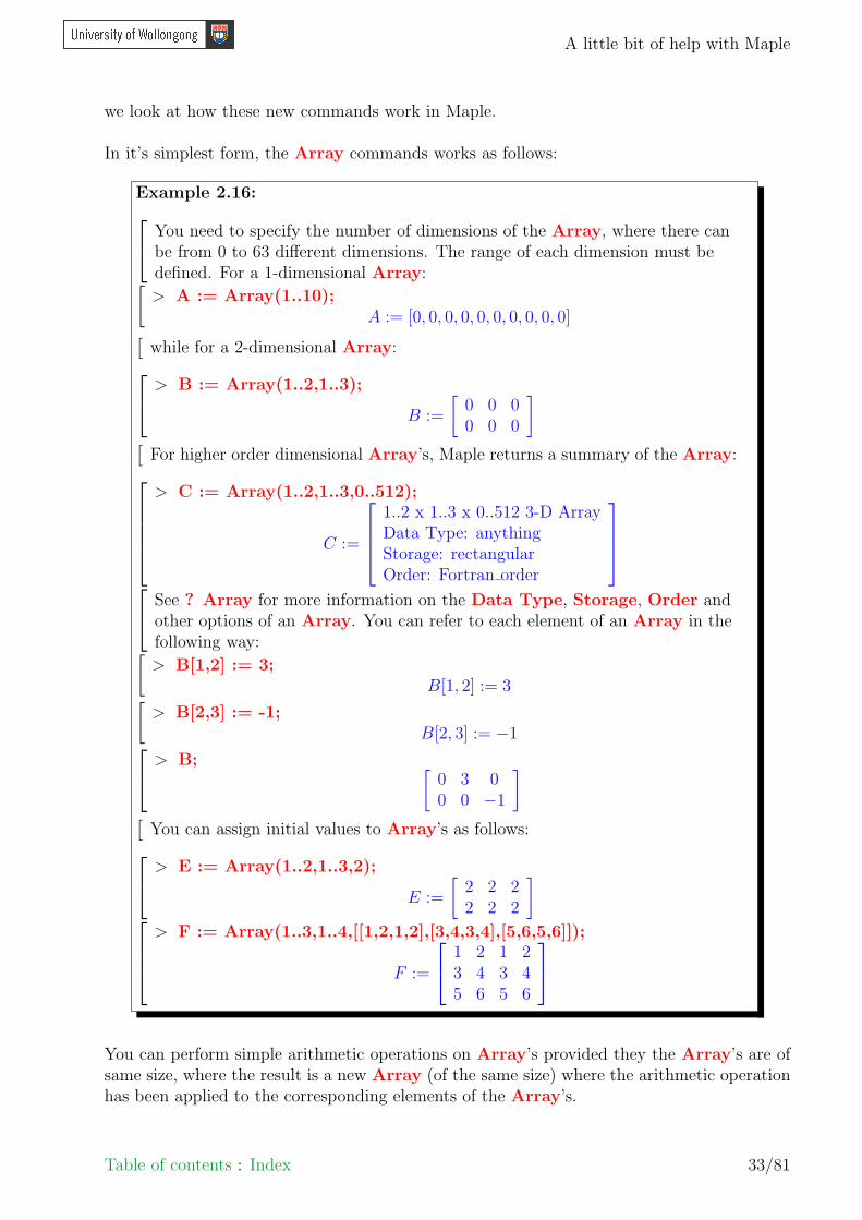
In it’s simplest form, the Array commands works as follows:

Example 2.16: You need to specify the number of dimensions of the Array, where there canbe from 0 to 63 different dimensions. The range of each dimension must bedefined. For a 1-dimensional Array:[> A := Array(1..10);

A := [0, 0, 0, 0, 0, 0, 0, 0, 0, 0][while for a 2-dimensional Array: > B := Array(1..2,1..3);

B :=

[0 0 00 0 0

][

For higher order dimensional Array’s, Maple returns a summary of the Array:> C := Array(1..2,1..3,0..512);

C :=

1..2 x 1..3 x 0..512 3-D ArrayData Type: anythingStorage: rectangularOrder: Fortran order

See ? Array for more information on the Data Type, Storage, Order and

other options of an Array. You can refer to each element of an Array in thefollowing way:[> B[1,2] := 3;

B[1, 2] := 3[> B[2,3] := -1;

B[2, 3] := −1 > B; [0 3 00 0 −1

][

You can assign initial values to Array’s as follows: > E := Array(1..2,1..3,2);

E :=

[2 2 22 2 2

]

> F := Array(1..3,1..4,[[1,2,1,2],[3,4,3,4],[5,6,5,6]]);

F :=

1 2 1 23 4 3 45 6 5 6

You can perform simple arithmetic operations on Array’s provided they the Array’s are ofsame size, where the result is a new Array (of the same size) where the arithmetic operationhas been applied to the corresponding elements of the Array’s.



Example 2.17:[Assume the Array’s B, E and F are as defined in the previous example, i.e., > B; [

0 3 00 0 −1

] > E; [

2 2 22 2 2

]

> F; 1 2 1 23 4 3 45 6 5 6

[

Then we can calculate: > B - 3*E; [−6 −3 −6−6 −6 −1

] > B*E; [

0 6 00 0 −2

] > %/%%; [

0 −2 00 0 2

7

][

Note that normal matrix multiplication does not work:[> B*F;

Error, (in rtable/Product) invalid arguments[Recall, that we also have the non-commutative multiplication operator ., i.e., > B . E; [

0 6 00 0 −2

][

so in terms of Array’s, * and . are the same.

Array’s are useful when you want to store, manipulate and manage multi-dimensional data.However, when you have one or two dimensional data (i.e., something which can be expressedas a vector or a matrix), then it is better to use the Vector and Matrix data structures,as there exists many useful commands in the LinearAlgebra package that can be used tomanipulate them.

The Vector data structure is useful when you want to perform matrix calculations on one-dimensional array’s. Vector’s differ to Array’s in that they are only one-dimensional andoperations on Vector’s must obey the usual linear algebra rules for matrices.



Example 2.18:[The are a number of ways to define Vector’s, including:> A := Vector(3); 0

00

> B := Vector(1..3,5);

B :=

555

[

> C := Vector[row]([1,2,3]);C := [1, 2, 3]

> E := Vector[column]([4,5,6]); 456

> F := 2*B;

E :=

101010

> B + F; 151515

[

> B + C;Error, (in rtable/Sum) invalid arguments[

Referring to an element of a Vector is similar to Array’s:[> C[2];

2[To convert a row vector into a column vector, or vice-versa, use the convertcommand:> G := convert(C,Vector[column]); 1

23

[

> type(G,Vector[column]);true

See ? Vector for some other ways to define a Vector and it’s elements. When specifying aVector, you can add the option of either [row] or [column], as shown in the above example.In these cases, the Vector is outputted and treated as either a row or column vector. Bydefault, Maple assumes the Vector is a column vector.



You can perform operations on Vector’s in the same way as Array’s – provided they are ofthe same dimension and type – except for multiplication.

Example 2.19:> B := Vector(1..3,5);

B :=

555

[

> C := Vector[row]([1,2,3]);C := [1, 2, 3]

> E := Vector[column]([4,5,6]); 456

[

The * multiplicative operator does not work for Vector’s, i.e.,[> B * E;

Error, (in rtable/Product) invalid arguments[> E * C;

Error, (in rtable/Product) invalid arguments[However, the . non-commutative multiplicative operator works are follows:[If you multiply two Vector’s of the same orientation, then the dot product ofthe two Vector’s is returned, i.e.,[> B.E;

75[> C . C;

14[If the two Vector’s are of different orientation, then the two vector’s aremultiplied according to the standard rules of matrix multiplication, i.e.,> E .C; 4 8 12

5 10 156 12 18

[

> C. E;32[

Note that the blank spaces around the . operator above do not matter, asMaple will ignore them when dealing with non-numbers.

To perform more complicated operations on Vector’s, you need to use commands from theLinearAlgebra package – we will see more about this later.

Note:An alternate way to define a Vector is to use the < > notation.

�



Example 2.20:> A := <1,0,1>;

A :=

101

[

> type(A,Vector);true

A Matrix is similar to a Vector, except that it can be one or two dimensional.

Example 2.21: > M := Matrix(2);

M :=

[0 00 0

] > N := Matrix(2,3);

N :=

[0 0 00 0 0

] > P := Matrix(1..2,1..3,5);

P :=

[5 5 55 5 5

] > Q := Matrix([[1,2,3],[4,5,6]]);

Q :=

[1 2 34 5 6

] > R := Matrix(2,3,symbol=m);

R :=

[m1,1 m1,2 m1,3

m2,1 m2,2 m2,3

]

Note:To refer to an element of a Matrix, you need to specify both the row and the column of theelement in the Matrix – even when the Matrix is one-dimensional.

�

Example 2.22: > Q := Matrix([[1,2,3],[4,5,6]]);

Q :=

[1 2 34 5 6

][

> Q[2,3];6[

> T := Matrix([3,5,7]);T := [3 5 7][

> T[1,2];5



You can perform simple arithmetic operations on Matrix’s in a similar manner to Array’sand Vector’s.

Example 2.23: > P := Matrix(1..2,1..3,5);

P :=

[5 5 55 5 5

] > Q := Matrix([[1,2,3],[4,5,6]]);

Q :=

[1 2 34 5 6

] > P - 2*Q; [

3 1 −1−3 −5 −7

][

To perform matrix multiplication, you need to use the . operator:> S := Matrix(3,2,[[1,-1],[2,1],[3,1]]);

S :=

1 −12 13 1

> Q . S; [

14 432 7

] > Q . P;

Error, (in LinearAlgebra:-MatrixMatrixMultiply) first matrix columndimension (3) <> second matrix row dimension (2)

To perform more complicated operations on Matrix’s, you need to use commands from theLinearAlgebra package – we will see more about this later.

Note:An alternate way to define a Matrix is to use the << > | < >> notation, where each< > defines a column of the Matrix.

�

Example 2.24:> A := <<1,0,1> | <2,1,3>>;

A :=

1 20 11 3

[

> type(A,Matrix);true

The Matrix command has many useful options, see ? Matrix for more information. Aparticularly useful option is the ability to define identity matrices, as given below:



Example 2.25:> M:=Matrix(3,3,shape=identity);

M :=

1 0 00 1 00 0 1

[

Because we have specified that M has shape=indentity, then we are unableto change the elements of M, i.e.,[> M[1,1] := 2;

Error, invalid assignment to identity diagonal[> M[1,2] := 3;

Error, invalid assignment of non-zero to identity off-diagonal

2.6 Series expansions

Maple provides the ability to easily calculate different types of series expansions. Two of themost commonly used series expansions in Maple are series and taylor.

Example 2.26:[The series command computes a truncated series expansion of an expressionabout a specified point for the specified order.[> S := series(exp(x),x=0,8 );

S := 1 + x + 12x2 + 1

6x3 + 1

24x4 + 1

120x5 + 1

720x6 + 1

5040x7 + O(x8)[

> series(cos(x),x=1,3);cos(1)− sin(1)(x− 1)− 1

2cos(1)(x− 1)2 + O((x− 1)3)[

The O() term denotes the order of the series expansion. To remove the orderterm, say in order to plot the expansion, use the convert command, i.e.,[> T := convert(S,polynom);

1 + x + 12x2 + 1

6x3 + 1

24x4 + 1

120x5 + 1

720x6 + 1

5040x7[

Note that if the series is expanded about infinity, then an asymptoticexpansion is generated.[> series(xˆ3/(xˆ4+4*x-5),x=infinity);

1x− 4

x4 + 5x5 + O

(1x7

)[The taylor command computes the Taylor series of an expression, and is arestriction of the more general series command[> taylor(cos(x),x=1,3);

cos(1)− sin(1)(x− 1)− 12cos(1)(x− 1)2 + O((x− 1)3)[

> taylor(sin(x),x);x− 1

6x3 + 1

120x5 + O(x6)

For more information, see ? series.



2.7 Simplifying and manipulation expressions

There are many commands that can be used to simplify and manipulate expressions. In thissection, some of the more common commands will be discussed.

Example 2.27:[Expressions can be factorized using the factor command.[> factor(6*xˆ2+18*x-24);

6(x + 4)(x− 1) > factor((xˆ3-yˆ3)/(xˆ4-yˆ4));x2 + xy + y2

(y + x)(x2 + y2)[You can factorize an equation in the same manner:[> eqn := yˆ2 - 1 = xˆ2 + 4*x + 4;

y2 − 1 = x2 + 4x + 4[> factor(eqn);

(y − 1)(y + 1) = (x + 2)2[Alternatively, you can factorize the left hand or the right hand side of anequation separately, by using the lhs and rhs commands.[> lhs(eqn);

y2 − 1[> rhs(eqn);

x2 + 2x + 4[> factor(lhs(eqn)) = factor(rhs(eqn));

(y − 1)(y + 1) = (x + 2)2

Note:The factor command cannot be used to factorize expressions that cannot be perfectly fac-torized.

�

Example 2.28:[The factor command will not recognize that x2 + 2x + 1 + y can be factoredas (x + 1)2 + y.[> eq := xˆ2 + 2*x + 1 + y;

x2 + 2x + 1 + y[> factor(eq);

x2 + 2x + 1 + y[To factor the equation, we need to use the student[completesquare]command. We will see more on this later.



There are times when you want to factorize the denominator or numerator of an expression.In this case, the commands denom and numer come in handy.

Example 2.29: > yeqn := (sin(x)ˆ2 + 2*sin(x) + 1)/(x - 1/x);

yeqn :=sin(x)2 + 2 sin(x) + 1

x− 1

x[> yeqn denom := denom(yeqn);

x− 1

x[> yeqn numer := numer(yeqn);

sin(x)2 + 2 sin(x) + 1 > factor(yeqn numer)/factor(yeqn denom);(sin(x) + 1)2x

(x− 1)(x + 1)[Of course, in this case, we can just use the factor command normally: > factor(yeqn);

(sin(x) + 1)2x

(x− 1)(x + 1)

See ? factor for more information.

The opposite of factorizing expressions is, of course, expanding expressions. To do this, usethe expand command.

Example 2.30:[> expand((x - 1)*(x + 1));

x2 − 1[> expand((x+1)/(x+2));

x

x + 2+

1

x + 2 For quotients of polynomials, only sums in the numerator are expanded –products and powers are left alone. See the normal command for dealing withquotients of polynomials. > expand(1/(x+1)/x);

1

(x + 1)x[The expand command can be used for more than just polynomials:[> expand(sin(x+y));

sin(x) cos(y) + cos(x) sin(y)[> expand(exp(a+ln(b)));

eab



See ? expand for more information.

If you have an expression that can be simplified using well-known simplification rules, thenyou can use the simplify command to do this. The simplify searches the expression forfunction calls, square roots, radicals, and powers, and then invokes the appropriate simplifi-cation procedures.

Example 2.31:[> simplify(4ˆ(1/2)+3);

5[> te1 := exp(a+ln(b*exp(c)));

te1 := e(a+ln(bec))[> simplify(te1);

bea+c

There are times when using the simplify command causes unwanted and unnecessary diffi-culties, because Maple considers the analytical issue of branches for multi-valued functions.In situations where such branches are not of interest, then various options can be applied.

Example 2.32:[> g:=sqrt(xˆ2);

g :=√

x2[> simplify(g);

csgn(x)x where csgn is the sign function for real and complex functions – see ? csgnfor more information. However, if we are only interested in the symbolicsimplification, then:[> simplify(g,symbolic);

x[Alternatively, we could have done:[> simplify(g,assume=real);

x[> simplify(g,assume=positive);

x

See ? simplify for more information.

To combine terms in sums, products, and powers into a single term, the combine commandis used. For many functions, the transformations applied by the combine command are theinverse of the transformations that are applied by the expand command.



Example 2.33:[> expand(sin(a+b));

sin(a) cos(b) + cos(a) cos(b)[> combine(sin(a)*cos(b) + cos(a)*sin(b));

sin(a + b)[> E := exp(x)ˆ2*exp(y);

E := (ex)2ey[> combine(E);

e2x+y

There may be times when you only want certain terms to be combined. To do this, you needto specify the appropriate options in the combine command.

Example 2.34:[> eqn := 4*sin(x)ˆ3+exp(y)*exp(x);

eqn := 4 sin(x)3 + eyex[> combine(eqn);

− sin(3x) + 3 sin(x) + ex+y[> combine(eqn,trig;

− sin(3x) + 3 sin(x) + exey[> combine(eqn,exp);

4 sin(x)3 + ex+y

When you want to collect together the coefficients of a variable or function in an equation,then you should use the collect command.

Example 2.35:[> f := a*ln(x)-ln(x)*x-x;

a ln(x)− ln(x)x− x[> collect(f,ln(x));

(a− x) ln(x)− x[When collecting coefficients, Maple does not automatically sort them into anyparticular order.[> g := 3*(x - 2) + x*(2 - 3*xˆ2);

g := 3x− 6 + x(2− 3x2)[> collect(g,x);

−6− 3x3 + 5x[To do so, you need to use the sort command.[> sort(collect(g,x));

−3x3 + 5x− 6



See ? sort for more information. When you want to collect more than one variable or func-tion in an expression, you do so by specifying a list of objects to be collected.

Example 2.36:[> p := x*y+a*x*y+y*xˆ2-a*y*xˆ2+x+a*x;

p := xy + axy + yx2 − ayx2 + x + ax[> collect(p, x);

(y − ay)x2 + (y + ay + 1 + a)x[> collect(p, [x,y]);

(1− a)yx2 + ((1 + a)y + 1 + a)x[> collect(p, [y,x]);

((1− a)x2 + (1 + a)x)y + (1 + a)x[Note that the order the objects are to be collected in will alter the output. Ifthis is not desired, then use the distributed option.[> collect(p, [x,y], distributed);

(1 + a)x + (1 + a)xy + (1− a)yx2

See ? collect for more information. Additionally, if you have a polynomial, then you can askMaple to pick out particular coefficients using the coeff command.

Example 2.37:[> p := 4*xˆ2 + 3*yˆ3 - 5;

4x2 + 3y3 − 5[There are two ways to pick out the coefficient of x2, i.e.,[> coeff(p,x,2);

4[> coeff(p,xˆ2);

4[> coeff(p,x,0);

3y3 − 5

See ? coeff for more information.

If you want all of the coefficients, then you can either use the coeff command manually foreach coefficient, or you can use the coeffs command.



Example 2.38:[> s := 3*vˆ2*yˆ2+2*v*yˆ3;

s := 3v2y2 + 2vy3[The coefficients of v can be picked out by:[> coeffs(s,v,’vt’);

2y3, 3y2[where vt specifies what the corresponding power of v is, i.e.,[> vt;

v, v2[We can pick out the coefficients of y in a similar manner:[> coeffs(s,y,’yt’);

2v, 3v2[> yt;

y3, y2

See ? coeffs for more information.

Alternatively, you may only want to select, or remove, certain terms from an expression. Todo so, use the select, remove and selectremove commands.

Example 2.39:[> f := 2*exp(a*x)*sin(x)*ln(y);

f := 2eax sin(x) ln(y)[> select(has, f, x);

eax sin(x)[> remove(has, f, x);

2 ln(y)[> selectremove(has, f, x);

eax sin(x), 2 ln(y)[> g := 2*exp(a*x)*sin(x)*ln(y) + cos(x)*exp(b*y) + 3;

g := 2eax sin(x) ln(y) + cos(x)eby + 3[> select(has,g,cos);

cos(x)eby[> remove(has,g,[cos,ln]);

3

For more information, see ? select, ? remove and ? selectremove.

We have seen previously that we can use the op and nops commands to manipulate elementsin a list. We can also use these commands in other expressions.



Example 2.40:[To know the number of terms in an equation, use the nops command, i.e.,[> f := expand(((x-4)*(xˆ2 + x - 3) + xˆ2*(x - 3))ˆ2);

f := 4x6 − 24x5 + 8x4 + 132x3 − 95x2 − 168x + 144[> nops(f);

7[To create a sequence of all the terms, use the op command, i.e.,[> op(f);

4x6,−24x5, 8x4, 132x3,−95x2,−168x, 144[To select the nth term of the expression, use:[> op(1,f);

4x6[> op(2,f);

−24x5[> op(3,f);

8x4[and so forth. Further, you can use the op command to find the next level ofterms, i.e.,[> op(4,f);

123x3[> op(op(4,f);

123, x3

If you want to substitute values, or expressions, into an equation or expression, use the subscommand.

Example 2.41:[> w := a*b + b - 3*c;

w := ab + b− 3c[> subs(a=2,w);

3b− 3c[> subs([a=0],w);

b− 3c[> subs([a=1],[b=2],w);

4− 3c[> subs([a=1, b=3],[b=2],w);

6− 3c



Example 2.42:[There is a difference between the eval and subs commands:[> z := 6*u*vˆ2 - 3*v + 3*exp(v - u);

z := 6uv2 − 3v + 3ev−u[> subs(u=2,v=2,z);

42 + 3e0[> eval(z,[u=2,v=2]);

45

For more information, see ? subs.

2.8 Printing, reading and writing

When creating programs, you will often want to print messages to the screen, or to a file. Inthis section, we are going to look at how to print data to the screen and write data to files.

The print command displays the values of the arguments of the command to the screen, andreturns NULL as the function value. The arguments are printed separated by a comma anda blank space.

Example 2.43:[> print(I,Love,Maths);

I, Love, Maths[> print(”This is a string”);

”This is a string”[> x := 42;

x := 42[> print(x);

42[> print(seq(i,i=1..10));

1, 2, 3, 4, 5, 6, 7, 8, 9, 10[The print commands returns no value. > y := print(4*xˆ2);

16y :=[

> y;

See ? print for more information.



The print command is fairly limited in the format of how the output appears. One alter-native is to use the printf command. To do so, you need to specify the format string thatdefines the format of the output, where for full details see ? printf. Some examples of theprintf command are given below.

Example 2.44:[To output strings, use the %s format:[> printf(”%s\n”,”This is cool!”);

This is cool![> printf(”%s %s %s\n”,This, is, ”cool!”);

This is cool![> x := 42;

x := 42[> printf(”The answer is x = %s”, convert(x,string));

The answer is x = 42[Alternatively, to print the number x = 42 without converting to a string, usethe %g format, i.e.,[> printf(”The answer is x = %g”, x);

The answer is x = 42

For full details on all the different types of formats, see ? printf. There a number of differentways to write data to a file. One of these is the fprintf command, which is related to theprintf command.

Example 2.45:> x := 23; y := -1/x;

x := 23

y :=−1

23[You first need to use the fopen command to open the file you want to printto, i.e., > fd := fopen(”temp file”, WRITE):

fprintf(fd, ”x = %d, y = %g”,x,y):fclose(fd): which will have written: x = 23, y = −0.0434783 to the file: temp file. The

location of this file will depends on a number of factors. To be certain of it’slocation, use: > fd := fopen(”C:/temp file”, WRITE):

fprintf(fd, ”x = %d, y = %g”,x,y):fclose(fd):[

where the file is located on the C: drive. Note that you must close the fileusing the fclose command – otherwise the file will appear empty.



For more information, see ? fprintf, fopen and fclose. Some other useful commands towrite data to a file include the writeline, writedata and writestat commands.

Example 2.46:[The writeline command writes a string to either the screen or to a file: > writeline(terminal,”This is a test”,”So is this”));

This is a testSo is this

26[The 26 is the number of characters returned from the writeline command. Tosuppress this, use the colon : instead. To write the strings to a file, use:[> writeline(”C:/whatever.txt”,”This is a test”,”So is this”):

fclose(”C:/whatever.txt”):[The writedata command can be used to numerical data to a file.[> A := [[0,1,3.4,2,5.3],[-3,1,5.6,2,4.5]];

A := [[0, 1, 3.4, 2, 5.3], [−3, 1, 5.6, 2, 4.5]][> writedata(”C:/A data.txt”,A,float):which writes

0 1 3.4 2 5.3

−3 1 5.6 2 4.5

to the file A data.txt, and is located on the C: drive. If[> B := [[x,1,3.4,2,5.3],[y,1,5.6,2,4.5]];;

B := [[x, 1, 3.4, 2, 5.3], [y, 1, 5.6, 2, 4.5]];[> writedata(”C:/B data.txt”,B,float);

Error, (in writedata) Bad data found x[because x and y are not numerical values. To get around this, you need tospecify the individual formats for each data, i.e.,[> writedata(”C:/B data.txt”,B,[string,integer,float,integer,float]);

fclose(”C:/B data.txt”):[The writestat command writes a string or an expression to a file. In someways, it is the more general form of both writeline and writedata.

For more information, see ? writedata, ? writeline and writestat. Another alternativeon how to write data to a file, is to use the writeto and appendto commands. Simply put,you use the writeto command to specify what file to want to start writing to, and then fromthis point onwards any commands executed in the Maple worksheet will have their outputwritten to the specified file. If you only want to append to a file that already has somethingin it, then use the appendto command, which will start writing at the end of the specified file.



Example 2.47:[> writeto(”C:/C data.txt”);[> y := xˆ2 - 2*x + 1;[> 3*4;[> writeto(terminal);[> y;

x2 − 2 ∗ x + 1[where the command writeto(terminal) tells Maple to write back to thescreen again.

See ? writeto and ? appendto for more information.

The opposite of writing is, of course, reading. To read data from a file, you can use readline,readdata or readstat, in a similar manner to how the write versions work.

Example 2.48:

Suppose that a file called SomeData.txt is located on the C: drive, andcontains:

1 2 3 4 5

6 7 8 9 0

To read the first column of this data, use:[> readdata(”C:/SomeData.txt”,1);

[1., 6.][where, unless told otherwise, Maple assumes the numbers are floats. Further,to read in all 5 columns:[> readdata(”C:/SomeData.txt”,1);

[[1., 2., 3., 4., 5.], [6., 7., 8., 9., 0.]]If instead SomeData.txt contains:

x 2 3 4 5

y 7 8 9 0

then to read in all the data, you need to specify the type of each column, i.e.,[> readdata(”C:/SomeData.txt”,[string,integer,float,integer,float]);

[[”x”, 2, 3., 4, 5.], [”y”, 7, 8., 9, 0.]]

For more information, see ? readdata, ? readline and ? readstat.

Finally, if you have a file that contains Maple commands, then you can tell Maple to execute



these commands by using the read command.

Example 2.49:

Suppose that a file called SomeCommands.txt is located on the C: drive, andcontains:

y := sin(x);

subs([z=y],zˆ2 - 1);

To get Maple to read in and execute these commands, use: > read ”C:/SomeCommands.txt”;y := sin(x)sin(x)2 − 1[

Note that the restart command will not be executed if Maple reads it in froma file


Chapter 3

Calculus

In this chapter, we look at how to calculate derivatives and integrals of expressions.

3.1 Differentiation

To calculate the partial derivative of an expression, use the diff command.

Example 3.1:[> diff(sin(x),x);

cos(x)[> diff(sin(x),y);

0[You can calculate higher order derivatives in a number of ways, i.e.,[> diff(diff(xˆ2 - 3*x + 4,x),x);

2[or,[> diff(xˆ2 - 3*x + 4,x,x);

2[or,[> diff(xˆ2 - 3*x + 4,[x,x]);

2[or,[> diff(xˆ2 - 3*x + 4,x$2);

2[where $ is operator for forming an expression sequence, i.e.,[> x$4;

x, x, x, x

52


For more information, see ? $ and ? diff. The $ operator is particularly useful when dealingwith higher order derivatives.

Example 3.2:[> z := sin(x)*cos(y);

z := sin(x) cos(y)[> diff(z,x$42,y$76);

− sin(x) cos(y)

The inert form of the diff command, is the Diff command.

Example 3.3: > Diff(f(x,y),[x,y]) = diff(sin(x*y),[x,y]);∂2

∂y∂xf(x, y) = − sin(xy)xy + cos(xy)

There is also a differential operator in Maple, namely the D command.

Example 3.4:[> D(sin);

cos[> D(cos);

− sin[To calculate higher order derivatives, use the @@ operator, i.e.,[> (D@@2)(sin);

− sin The D operator is particularly useful when you want to specify the derivativeof an expression evaluated at a point, i.e., when you need to specify initial orboundary conditions:[> D(f)(0) = 0;

D(f)(0) = 0[or, in other words, > convert(D(f)(0) = 0,diff);(

d

dt1f(t1)

)∣∣∣∣t1=0

= 0

The D operator can also be used for partial derivatives, where you need to specify whichindependent variable you want to differentiate with respect to.



Example 3.5:> D[1](F)(x,y)

convert(%,diff);D1(F )(x, y)

∂

∂xF (x, y)

> D[2](F)(x,y)convert(%,diff);

D2(F )(x, y)

∂

∂yF (x, y)[

To calculate higher order partial derivative operators, consider> D[1,1,2](F)(x,y)

convert(%,diff);D1,1,2(F )(x, y)

∂3

∂y∂x2F (x, y)

For more information, see ? D and ? @@.

3.2 Integration

The opposite of differentiation is, of course, integration. To integrate an expression, use theint command.

Example 3.6:[To calculate an indefinite integral:[> int(sin(x),x);

− cos(x)[Note that no constant of integration appears in the result. To calculate adefinite integral:[> int(sin(x),x=0..Pi);

2[> int(sin(x),x=0..pi);

1− cos(π)[To calculate a double integral, you need to repeat the int command, i.e.,[> int(int(sin(x),x),x);

− sin(x)



Note:There is no shorthand way to represent double, triple and higher order integrals – you mustrepeat the int command for each integral.

�

Example 3.7: > int(x,x);x2

2[If we try a shorthand way, similar to higher order derivatives, then Mapleeither ignores the extra input or returns an error, i.e., > int(x,x,x);

x2

2 > int(x,x$3);x2

2[> int(x,[x,x,x,x]);

Error, (in int) wrong number (or type) of arguments

The inert form of int is the Int command.

Example 3.8: > Int(f(x),x=a..b); ∫ b

a

f(x)dx > eqn := Int(Int(x*y,x),y);

eqn :=

∫∫xy dxdy[

To get Maple to evaluate the Int command, use the value command, i.e., > value(eqn);x2y2

4

Note:The value command can be used to force Maple to evaluate inert commands, such as Int,Diff, Limit, Product and Sum, by applying the lowercase versions, i.e., int, diff, limit,product and sum.

�

Sometimes Maple cannot evaluate an integral analytically. In this case, Maple will simplyreturn your call. However, in such situations, if there are no non-numeric values then you canask Maple to determine a numerical approximation to the integral using the evalf command.



Example 3.9: > MyInt := int(sin(cos(sin(x))),x=0..Pi);

MyInt :=

∫ π

0

sin(cos(sin(x))) dx[To determine a numerical approximation to the above integral, use the evalfcommand, i.e.,[> evalf(MyInt);

2.147394008


Chapter 4

Solving equations

In this chapter, we look at how to use Maple to solve algebraic, differential and recurrenceequations.

4.1 Algebraic equations

To solve algebraic equations, use the solve command.

Example 4.1:[> eqn := f = m*a;

eqn := f = m a[To solve eqn for a:[> solve(eqn,a);

f

m[Note that Maple returns what a is equal to – it does not return an equation. Ifthere is more than one solution, Maple will return a sequence of solutions, i.e.,[> eq := xˆ4-5*xˆ2+6*x=2;

eq := x4 − 5x2 + 6x = 2[> sols := solve(eq,x);

sols := 1, 1,√

3− 1,−1−√

3[> sols[3]; √

3− 1[You can use the solve command to solve a system of equations, i..e,> e1 := 4*x - 5*y = 3;

e2 := x + 7*y = 0;e1 := 4x - 5y = 3e2 := x + 7y = 0[

> solve({e1,e2},{x,y});

{y =−1

11, x =

7

11}

57


Note:If you specify the variables to be solved for using a set, as in the above example, then Maplewill return the answer in any order. In the above example, the order of the variables werespecified by {x,y}, but Maple returned the answer with y first, and then x. However, if youexecute the solve command again, then Maple may return the answers in a different order.This is particularly true for large systems of equations. If you want Maple to always returnthe solution in a desired order, then specify the order of the variables using a list (see examplebelow).

�

Example 4.2:> eqn1 := 3.2*x + 1.3*y + 4.2*z = 5;

eqn2 := 8.7*x + 19*y + 11.2*z = 94;eqn3 := x + y/4 + z = 1;

eqn1 := 3.2*x + 1.3*y + 4.2*z = 5eqn2 := 8.7*x + 19*y + 11.2*z = 94

eqn3 := x + y/4 + z = 1[> solve({eqn1, eqn2, eqn3}, [x, y, z]);

[[x = 0.4969502408, y = 5.187800963, z = −0.7939004815]][> solve({eqn1, eqn2, eqn3}, [x, z, y]);

[[x = 0.4969502408, z = −0.7939004815, y = 5.187800963]][> solve({eqn1, eqn2, eqn3}, [y, x, z]);

[[y = 5.187800963, x = 0.4969502408, z = −0.7939004815]] Note that because some of the coefficients of the variables in the aboveequations are floating point numbers, then Maple will automatically convertthe answers to floating point numbers.

See ? solve for more information. If you have used the solve command to find the analyticalsolutions to an equation, but you want to know the floating point value of the solutions, thenconsider the following two methods.

Example 4.3:[> eq := xˆ4-5*xˆ2+6*x-2;

eq := x4 − 5x2 + 6x− 2[> sols := solve(eq,x);

sols := 1, 1,√

3− 1,−1−√

3[If you want a floating point approximation of the solution, then you can eitheruse evalf, i.e.,[> evalf(solve(eq,x));

1., 1., 0.732050808,−2.732050808[or you can use the fsolve command.[> fsolve(eq,x);

−2.732050808, 0.732050808, 1., 1.



The fsolve command works in pretty much the same way as the solve command. If theequation is a polynomial, then Maple will return all real roots, by default. If the equationis not a polynomial, then Maple will return a single root of the equation. There are someoptions to try to get Maple to solve for more roots.

Example 4.4:[> fsolve(sin(x) = 1,x);

1.570796327[To get Maple to solve for a different root, either specify a range, i.e.,[> fsolve(sin(x) = 1,x=-6..1);

−4.712388980[or use the avoid option and specify a starting point, i.e.,[> fsolve( sin(x) = 1,x=8,avoid={x=1.570796327, x=-4.712388980});

7.853981636[If you want all the roots of a polynomial, where some of the roots are complex,then you need to specify the complex option, i.e.,[> polynomial := 23*xˆ5 + 105*xˆ4 - 10*xˆ2 + 17*x;

polynomial := 23x5 + 105x4 − 10x2 + 17x[> fsolve(polynomial);

−4.536168981,−0.6371813185, 0. > fsolve(polynomial, x, complex);-4.536168981, -0.6371813185, 0., 0.3040664543 - 0.4040619058 I,

0.3040664543 + 0.4040619058 I[Note that if Maple cannot find a solution, then NULL is returned, i.e.,[> fsolve(xˆ2 + 1 = 0,x);

For more information, see ? fsolve. An alternate to using the solve command to determinethe analytical solution of a system of equations, is the eliminate command.

Example 4.5:> eqn1 := xˆ2+yˆ2-1;

eqn2 := xˆ3-yˆ2*x+x*y-3;eqn1 := x2 + y2 − 1

eqn2 := x3 − y2x + xy − 3 > eliminate({ eqn1, eqn2 },x);[{x =

3

−2y2 + y + 1}, {−7y4 + 4y6 + 6y3 − 4y5 + 4y2 − 2y + 8}

][

where Maple returns one possible expression for the desired variable andwhatever equations are left when the elimination is made.



See ? eliminate for more information.

To determine integer-valued solutions of an equation, use the isolve command.

Example 4.6:[> isolve(xˆ2 - x - 6);

{x = −2}, {x = 3}[> isolve(3*x-4*y=7);

{x = 5 + 4 Z1, y = 2 + 3 Z1}[where Z1 is an arbitrary constant. If isolve cannot determine aninteger-valued solution, then NULL is returned, i.e.,[> isolve(x2̂=3);

For more information, see ? isolve. Additionally, if you want to find integer-valued solutions(mod n), then use the msolve command.

Example 4.7:[> msolve(3*x-4*y=1,7*x+y=2,19);

{y = 11, x = 15}[> msolve(2ˆi=3,19);

{i = 13 + 18 Z1}

See ? msolve for more information.



4.2 Differential equations

In this section we will look at how to solve differential equations. For ordinary differentialequations, use the dsolve command.

Example 4.8: > ode := diff(y(x),x,x) = 2*y(x) + 1;

ode :=d2

dx2y(x) = 2y(x) + 1[

> dsolve(ode);

y(x) = e(√

2x) C2 + e(−√

2x) C1− 1

2[where C1 and C2 are arbitrary constants of integration. You can specifyconditions to determine the constants of integration, i.e.,[> ics := y(0)=1, D(y)(0)=0;

ics := y(0) = 1, D(y)(0) = 0[> sol := dsolve({ode, ics});

sol := y(x) =3

4e(√

2x) +3

4e(−

√2x) − 1

2[To test to see if the solution satisfies the ode, use the odetest command, i.e.,[> odetest(sol,ode);

0 where if zero is returned, then the solution satisfies the ode. If you also wantto check that the solution satisfies the initial conditions, then specify a list ofequations that you want to check whether the solution satisfies, i.e.,[> odetest(sol,[ode, ics]);

[0, 0, 0][where the first zero corresponds to the ode, the second zero to the first initialcondition and the third zero to the second initial condition, respectively.

Note:In the above example, to specify initial conditions that contain a derivative, the D operatoris used.

�

For more information, see ? dsolve. Maple can also determine numerical solutions to odesusing the numeric option in dsolve, i.e.,

Example 4.9: > deq1 := diff(y(x),x) + sin(x)*y(x) = 0;

deq1 :=

(d

dxy(x)

)+ sin(x)y(x) = 0



[> ics := y(0) = 1;

ics := y(0) = 1[The analytical solution is given by > dsol := dsolve(deq1, ics);

dsol := y(x) =ecos(x)

e[while the numerical solution is given by[> dsol N := dsolve(deq1, ics,numeric);

dsol N := proc(x rkf45)...end proc where x rkf45 denotes the numerical solution is using a Fehlberg fourth-fifthorder Runge-Kutta method with degree four interpolant, and theproc ... end proc defines a procedure (which we will see more about later).To see the numerical solution:[> dsol N(0);

[x = 0., y(x) = 1.][> dsol N(0.1);

[x = 0.1, y(x) = 0.995016612435748794][> dsol N(2);

[x = 2., y(x) = 0.242647315785959495][Alternatively, you can use the output=listprocedure option, i.e.,[> dsol N2 := dsolve(deq1, ics,numeric, output=listprocedure);

dsol N2 := [x = (proc(x)...end proc), y(x) = (proc(x)...end proc)][> f := eval(y(x),dsol N2);

f := proc(x)...end proc[> f(2);

0.242647315785959495

Note:To plot the numerical solution, Maple provides the odeplot command within the plots pack-age (see next chapter).

�

To solve partial differential equations, use the pdsolve command.

Example 4.10: > PDE := x*diff(f(x,y),y)-y*diff(f(x,y),x) = 0;

PDE := x

(∂

∂yf(x, y)

)− y

(∂

∂xf(x, y)

)= 0[

> pdsolve(PDE);f(x, y) = F1(x2 + y2)[

where F1(x2 + y2) is an arbitrary function of x2 + y2.



The pdsolve command has many options to try to help Maple solve the pde. For example,you can suggest the form of the solution.

Example 4.11: > PDE := S(x,y)*diff(S(x,y),y,x) + diff(S(x,y),x)*diff(S(x,y),y) = 1;

PDE := S(x, y)

(∂2

∂y∂xS(x, y)

)+

(∂

∂xS(x, y)

)(∂

∂yS(x, y)

)= 1[

If we use pdsolve without any hints, then we get: > pdsolve(PDE);

(S(x, y) = F1(x) F2(y))&where

[{ d

dxF1(x) =

c1

F1(x),

d

dyF2(y) =

1

2

1

F2(y) c1

}]

[However, if we suggest a form of the solution, then[> pdsolve(PDE,HINT=P(x,y)ˆ(1/2));

S(x, y) =√

F2(x) + F1(y) + 2xy[where F1 and F2 are arbitrary functions of their arguments.

Note:You can also use pdsolve to try to solve a system of partial differential equations.

�

Maple can also be used to find a numerical solution to a partial differential equation.

Example 4.12:[Consider the pde: > PDE := diff(u(x,t),t)=-diff(u(x,t),x);

PDE :=∂

∂tu(x, t) = −

(∂

∂xu(x, t)

)[

subject to the initial-boundary conditions:[> IBC := u(x,0)=sin(2*Pi*x),u(0,t)=-sin(2*Pi*t);

IBC := {u(x, 0) = sin(2πx), u(0, t) = − sin(2πt)}[Then the numerical solution is given by[> pds := pdsolve(PDE,IBC,numeric,time=t,range=0..1);

pds := module()export plot, plot3d, animate, value, settings; ...end module[Note that the numerical solution of a pde returns a module, not a proc likethe numerical solution of an ode. Please see later for more information onmodule’s.



[To examine the numerical values of the solution, use the values option, i.e.,> pds:-value(t=0)(0);

pds:-value(t=0)(1);[x = 0., t = 0., u(x, t) = 0.]

[x = 1., t = 0., u(x, t) = −0.244929359829470494 10−15] The above values correspond to t = 0 with x = 0 and x = 1. To plot thenumerical solution, you don’t need the odeplot command, but instead youcan use the plot option, i.e.,

> p1:=pds:-plot(t=0,numpoints=50):p2:=pds:-plot(t=1/8,numpoints=50,color=blue):p3:=pds:-plot(t=1/4,numpoints=50,color=green):plots[display](p1,p2,p3);

For more information, please see ? pdsolve, ? pdsolve, system and ? pdsolve, numeric.

4.3 Recurrence equations

To solve recurrence relations, use the rsolve command.

Example 4.13:[> rsolve(f(n) = -3*f(n-1) - 2*f(n-2), f(k));

(2f(0) + f(1))(−1)k + (−f(0)− f(1))(−2)k[You can apply initial conditions, i.e.,[> rsolve(f(n) = -3*f(n-1) - 2*f(n-2), f(1..2)=1, f);

f(n) = −3(−1)n + (−2)n[You can make a procedure of the solution, i.e., > rr := rsolve(s(n) = 2*s(n-1), s(0)=1, s, ’makeproc’);

rr := proc (n)if 1 < nargs then (′procname′)(args) else expand(2n)end if end proc[

> rr(0), rr(1), rr(2), rr(3);1, 2, 4, 8


Chapter 5

Some useful packages

In this chapter we will look at some packages that contain some commands that you may finduseful in Maple.

To include a package into Maple, you need to use the with command.

Example 5.1:[To include the plots package, use

> with(plots);Warning, the name changecoords has been redefined

[Interactive, animate, animate3d, animatecurve, arrow, changecoords,complexplot, complexplot3d, conformal, conformal3d, contourplot,

contourplot3d, coordplot, coordplot3d, cylinderplot, densityplot, display,display3d, fieldplot, fieldplot3d, gradplot, gradplot3d, graphplot3d,implicitplot, implicitplot3d, inequal, interactive, interactiveparams,

listcontplot, listcontplot3d, listdensityplot, listplot, listplot3d, loglogplot,logplot, matrixplot, multiple, odeplot, pareto, plotcompare, pointplot,

pointplot3d, polarplot, polygonplot, polygonplot3d, polyhedra supported,polyhedraplot, replot, rootlocus, semilogplot, setoptions, setoptions3d,spacecurve, sparsematrixplot, sphereplot, surfdata, textplot, textplot3d,

tubeplot ]Note that if you use the semi colon ;, then you will see a list of all thecommands available in the package. Also, in this case, a warning message isgiven saying that this package has redefined a command that already exists inMaple – this is something to be kept in mind if you need to use either thestandard or the new definition of this command.[To include only a particular command, say the listplot command, use[> with(plots, listplot);

[listplot][Alternative, if you only want to use a command once or twice, then you canuse the [ ] notation, i.e.,[> plots[listplot]([seq([i,sin(i)],i=0..10)]):

65


5.1 plots

The plots package contains over fifty commands that can be used to plot various Maple ex-pressions and data structures. A brief description of some of the more useful and commonlyneeded commands are presented below.

The display and display3d commands can be used to plot multiple plots in the same plot.Example 4.12 above provides an example of this for display.

Example 5.2:[> with(plots):

> F:=plot3d(sin(x*y), x=-Pi..Pi, y=-Pi..Pi):G:=plot3d(x + y, x=-Pi..Pi, y=-Pi..Pi):H:=plot3d([2*sin(t)*cos(s), 2*cos(t)*cos(s), 2*sin(s)], s=0..Pi, t=-Pi..Pi):display([F, G, H]);

For more information, see ? plots[display]. To plot a list of points, or an array of data, thelistplot command is very useful.

Example 5.3:[> t := Array([seq(i,i=1..10)]);

t := [1, 2, 3, 4, 5, 6, 7, 8, 9, 10]

> plots[listplot]([seq([t[i],sin(t[i])],i=1..10)],color=pink,thickness=3);



See ? plots[listplot] for more information. The command dsolve can be used to determinethe numerical solution to and ordinary differential equation. To plot the resulting solution,you can use the odeplot command.

Example 5.4:[> with(plots, odeplot);

[odeplot][> p:= dsolve(D(y)(x) = y(x), y(0)=1, type=numeric, range=-5..2):

> odeplot(p,thickness=3);

[If the range is not specified in the dsolve command, then you need to do so inthe odeplot command, i.e.,[> p2 := dsolve( diff(y(x),x) = sin(x*y(x)),y(0)=2,y(x),type=numeric):

> odeplot(p2,[x,y(x)],0..6,thickness=3);

See ? plots[odeplot] for more information. Another way to plot a polar curve, is to use thepolarplot command.

Example 5.5:[To plot a circle of radius 1:

> polarplot(1);



[To plot x = cos θ and y = sin θ, use the similar format to the plot commandwith coords=polar option, i.e.,

> polarplot([cos(t),sin(t),t=0..2*Pi],color=gold,thickness=2);

For more information, see ? plots[polarplot]. To plot a list of data in order to create aclosed shaped, you can use the polygonplot and and polygonplot3d.

Example 5.6:

> onepoly := [[0,0],[0,1],[1,1] ,[1,0]];polygonplot(onepoly,thickness=3);

onepoly := [[0, 0], [0, 1], [1, 1], [1, 0]]

[To create a polygon, consider:

> ngon := n − > [seq([cos(2*Pi*i/n), sin(2*Pi*i/n)], i = 1..n)]:polygonplot(ngon(5),color=BLUE);

[Similar closed shaped can be created in three-dimensions usingpolygonplot3d.

See ? polygonplot and ? polygonplot3d for more information. To write words, symbolsand sentences onto plots, Maple provides the textplot command.



Example 5.7:

> p := plot(sin(x),x=-Pi..Pi):delta := 0.05:t1 := textplot([Pi/2,1+d,‘Local Maxima (Pi/2, 1)‘],align=ABOVE):t2 := textplot([-Pi/2,-1,‘Local Minima (-Pi/2, -1)‘],align=BELOW):display(p,t1,t2,thickness=3);

For further information, see ? plots[textplot].

5.2 LinearAlgebra

We have seen how to perform simple operations on Vector’s and Matrix’s. Maple providesthe LinearAlgebra package with over one hundred commands to manipulate Vector’s andMatrix’s.

Example 5.8:[> with(LinearAlgebra): > P := Matrix(1..2,1..3,5);

P :=

[5 5 55 5 5

] > Q := Matrix([[1,2,3],[4,5,6]]);

Q :=

[1 2 34 5 6

][

To transpose a Matrix, use the Transpose command, i.e.,> T := Transpose(Q);

T :=

1 42 53 6

[

To multiply to Matrix’s together, use the Multiply command, i.e., > Multiply(Q,T); [14 3232 77

]



For more information, see ? LinearAlgebra[Transpose] and ? LinearAlgebra[Multiply].To determine the eigenvalues and eigenvectors of a given Matrix, use the Eigenvalues andEigenvectors commands.

Example 5.9:> with(LinearAlgebra):

A := << −1,−3,−6 > | < 3, 5, 6 > | < −3,−3,−4 >>;

A :=

−1 −3 −63 5 6

−3 −3 −4

> Eigenvalues(A); −422

> (v, e) := Eigenvectors(A);

v, e :=

−422

,

12−1 1

12

0 11 1 0

so the Eigenvectors command returns a Vector containing the eigenvalues

and a Matrix containing the corresponding eigenvectors as the columns of theMatrix. Thus, checking that Ax = λx, i.e.,> Multiply(A,e[1..3,1]) = Multiply(v[1],e[1..3,1]); −2

−24

=

−2−2

4

[

where here λ is[> v[1];

−4[and x is the corresponding eigenvector, i.e.,> e[1..3,1];

1212

1

Note:The Multiply command can also be used to multiply Matrix’s with Vector’s and scalars,as demonstrated above.

�

See ? LinearAlgebra[Eigenvalues] and ? LinearAlgebra[Eigenvectors] for more infor-mation.



5.3 PDEtools

The PDEtools package is a collection of commands and routines to help find analytical so-lutions to partial differential equations. However, here we present a couple of the commandsthat can be utilized elsewhere in Maple.

The dchange command can be used to change the variable in mathematical expressions.

Example 5.10:[> with(PDEtools): > PDE := diff(f(x,y),x) + g(x,y) + diff(f(x,y),y)=0;

PDE :=

(∂

∂xf(x, y)

)+ g(x, y) +

(∂

∂yf(x, y)

)= 0

> tr := x = r + s, y = r - s:dchange(tr,PDE); (

∂

∂rf(r, s)

)+ g(r, s) = 0 > II := Int(xˆ2,x=0..1);

II :=

∫ 1

0

x2dx > dchange(x=sin(y),II); ∫ π

2

0

sin(y)2 cos(y)dy

For more information, see ? PDEtools[dchange]. Another convenient command is thedeclare command.

Example 5.11:[It can be easier to read the Maple output if looks more compact, i.e.,> with(PDEtools):

declare(y(x), prime=x);y(x) will now be displayed as y

derivatives with respect to x of functions of one variable will now bedisplayed with ’[

so thatd

dxy(x) now looks like[

> diff(y(x),x);y′ > ode := diff(diff(y(x),x),x)*diff(y(x),x)*y(x)*f(x)-2*diff(y(x),x)ˆ3*xˆ6

+ 2*diff(y(x),x)ˆ2*y(x)*diff(g(x),x) + y(x)ˆ5;ode := y′′y′yf(x)− 2y′3x6 + 2y′2yg′ + y5



[You can tell Maple to toggle between using the compact form and the fullform, using the OFF and ON options, i.e.,> OFF;

ode;(d2

dx2y(x)

)(d

dxy(x)

)y(x)f(x)−2

(d

dxy(x)

)3

x6+2

(d

dxy(x)

)2

y(x)

(d

dxg(x)

)+y(x)5 > ON;

ode;y′′y′yf(x)− 2y′3x6 + 2y′2yg′ + y5

For more information, see ? PDEtools[declare].


Chapter 6

Programming in Maple

In this chapter, we look at how to use Maple to create functions and programs. The simplestway to create a function is by using the −> operator.

Example 6.1:[> f := x −> 3*x + 5;

f := x−> 3x + 5[> f(2);

11[> g := (x,y) −> sin(x)*cos(y) + x*y;

g := (x, y)−> sin(x) cos(y) + xy[> g(Pi/2, Pi);

−1 +1

2π2

See ? −> for more information.

6.1 Procedures

More advanced functions can be created using the proc command. This command can havenumerous arguments, but returns only one value (which may be assigned to some name).

Example 6.2:

> lc := proc( s, u, t, v )description ”linear combination of the arguments”;local lincom;lincom := s * u + t * v;return lincom

end proc;lc := proc (s, u, t, v) local lincom; description ”linear combination of

the arguments”; lincom := s*u + t*v; return lincom end proc[Notice that the last statement before the end proc does not need to have acolon : or a semi-colon ;.

73


Note:When writing programs and procedures, it is good programming practice to indent your codeto make it easier to read. Further, you can use blank lines to enhance the readability of yourcode. Finally, you should include comments in your code telling the reader what you aredoing. Comments can be inserted using the # command.

�

Example 6.3:

> DiffProd := proc(func1, func2, var)description ”Calculates the derivative of the product of the

two functions, func1 and func2, with respect to ’var’.”:

local Dfunc1, Dfunc2, answer:

Dfunc1 := diff(func1,var): # derivative of func1 w.r.t varDfunc2 := diff(func2,var): # derivative of func2 w.r.t var

# calculate derivative of product using product ruleanswer := Dfunc1*func2 + func1*Dfunc2:

return answerend proc;

DiffProd := proc (func1, func2, var)local Dfunc1, Dfunc2, answer;description ”Calculates the derivative of the product of th e two func-tions, func1 and func2, with respect to ’var’.”;

Dfunc1 := diff(func1, var); Dfunc2 := diff(func2, var); answer :=Dfunc1*func2 + func1*Dfunc2; return answerend proc[

> ans := DiffProd(sin(x),cos(x),x);ans := cos(x)2 − sin(x)2[

> diff(sin(x)*cos(x),x);cos(x)2 − sin(x)2[

> combine(ans);cos(2x)

Note:If Dfunc1, Dfunc2 and answer had not been defined as local (or global) variables, thenMaple would print a warning message to the screen saying that they have implicitly been de-fined as local variables. It is good programming practice to create code that does not produceany error or warning messages.

�

For more information, see ? proc.



6.2 Modules

Procedures can generally only be used to return one result. If you want multiple results re-turned, then use the module command.

Example 6.4:[If you have two numbers, a and b, and you want to know a + b mod 5 anda× b mod 5, then consider:> z5 := module()

export plus, times;plus := (a,b) −> a + b mod 5;times := (a,b) −> a * b mod 5;

end module;z5 := module () export plus, times; end module[

where plus and times have been defined as the results to be exported. Toaccess these results, you need to use the :- operator, i.e.,[> z5:-plus(2,4);

1[> z5:-times(2,4);

3

Note:We saw an example of a module, when we looked at the pdsolve command.

�

See ? module for more information.

6.3 If statements

When writing programs, it is common to want to test to see if an expression is true, and thenexecute some other statements depending on the value of the first expression. Maple providesthe if statement for this purpose. There is more than one representation of the if statement,due to optional arguments.

Example 6.5: > a := 3;b := 5;

a := 3b := 5[

> if a > b then a else b end if;5



> if b - a <> 0 then

c := b - aelse

c := a - bend if;

c := 2

> if c < a and c < b thena - c;b - c

elif c < a and c > b thena - c;c - b

elsea + b - c

end if;13[

The elif command above stands for ‘else if’.

Note:The last statement before either an else, elif or end if statement does not have to have acolon : or a semi-colon ;.

�

The operator form of the if statement is given by the ‘if‘ operator.

Example 6.6:[> a := 3; b := 5;

a := 3b := 5[

> 5*(Pi + ‘if‘(a > b,a,b));5π + 25

For more information, see ? if.

6.4 For statements

To repeat an expression, use the for statement. There is more than one representation of thefor statement, due to optional arguments.



Example 6.7:

> summ := 0;for i from 1 to 10 do

summ := summ + iend do;

summ := 0summ := 1summ := 3summ := 6summ := 10summ := 15summ := 21summ := 28summ := 36summ := 45summ := 55[

If you don’t want to see each step, then use a colon : at the end of the end docommand.

Note:If you nest for statements, then Maple will not show the output for each step – even if youuse a semi-colon ;. If you want to see the output, you need to use commands like print,writeline, etc.

�

Example 6.8:> for i from 1 by 2 while i <= 100 do

for j in [1,24,3,-6,0,2] doi*j

end do;end do;[

However, if you replace i*j by print(i*j), then each step will be printed to thescreen (not shown here as there are 300 lines of output!).

See ? for for more information.


Index

! , 6

!!! , 6+, 7−, 7/, 7<, 7<=, 7<>, 7>, 7>=, 7Γ, see GAMMA∗, 7∗∗, 7∞, 11||, 19’, 10->, 73:-, 75:=, 9#, 74$, 52%, see ditto%%, see ditto%%%, see dittoˆ , 7‘, 18

abs, 13add, 23and, 7appendto, 49Array, 32

Data Type, 33Order, 33Storage, 33

assign, see :=, 21

cat, 19, 21coeff, 44coeffs, 44collect, 43

distributed, 44

combine, 42command, 65commands

case sensitive, 6executing, 6

complex number, see Iconvert, 21

list, 17set, 17

cos, 23csgn, 42

Ddifferential operator, 53initial conditions, 61

dchange, 71declare, 71delay evaluation, see ’denom, 41Diff

evaluating Diff, 55inert form of diff, 53

diff, 52Digits, 13display, 66ditto, see operatorsdsolve, 61

numeric, 61plotting numerical solution, 67

Eigenvalues, 70Eigenvectors, 70eliminate, 59end of statement

colon :, 6seimcolon ;, 6

eval, 12evalb, 12evalc, 12evalf, 11

evaluating an integral numerically, 55numerical value of solve, 58

78


evaluationat a point, 12boolean, 12complex, 12floating point, see evalf

executing a statementhow to, 6no output, 6

execution group, 6exp, 11, 23expand, 41

factor, 40fclose, 48fopen, 48for, 76fprintf, 48fractions, 12fsolve, 59

avoid, 59complex, 59

GAMMA, 24

help?, 7in-built support pages, 7

I, 11if, 75implies, 7index, 32indexed, see nameinfinity, see ∞initial functions and constants, 11inserting new input prompts, 6Int

evaluating Int, 55inert form of int, 55

int, 54intersect, 7isolve, 60

lhs, 40Limit

evaluating Limit, 55inert form of limit, 26

limit, 26linalg

matrix, 32LinearAlgebra, 34, 69

Eigenvalues, 70Eigenvectors, 70Multiply, 69Transpose, 69

list, 15ln, 11, 23

maple functons, see initial functions and con-stants

Matrix, 32, 37<< > | < >>, 38indentity, 38

member, 7minus, 7module, 63, 75msolve, 60mul, 24Multiply, 69

name, 18indexed, 19symbol, 19

nops, 16, 45normal, 41not, 7number of digits, see Digitsnumer, 41

odeplot, 67odetest, 61op, 16, 45operators

ditto, 9logical, 7mathematical, 7relational, 7set, 7

or, 7

parse, 21PDEtools, 71

dchange, 71declare, 71

pdsolve, 62Pi, see pipi

difference between pi and Pi, 11plot, 27

axes, 27boxed, 27



frame, 27none, 27normal, 27

color, 27coords, 31labeldirections, 27labels, 27linestyle, 28list of points, 28multiple functions, 30numpoints, 28options, 28parametric plots, 29polar, 30thickness, 28

plot3d, 32plots, 62, 66

display, 30, 66display3d, 66odeplot, 62, 67polygonplot, 68polygonplot3d, 68spacecurve, 32textplot, 68

polygonplot, 68polygonplot3d, 68print, 47printf, 48proc, 73Product

evaluating Product, 55inert form of product, 25

product, 24

read, 51readline, 50remove, 17, 45restart, 10

not executed, 51rhs, 40rsolve, 64

select, 17, 45selectremove, 45seq, 18series, 39set, 15sign, 14simplify, 42

symbolic, 42

sin, 23solve, 57sort, 43sqrt, 23

the square root function, 13starting Maple, 4string, 21student[completesquare], 40subs, 46subset, 7Sum

evaluating Sum, 55inert form of sum, 25

sum, 23symbol, see name

tan, 23taylor, 39textplot, 68Transpose, 69type, 21

unassign, 10union, 7

value, 25, 55Vector, 32, 34

< >, 36column, 35dot prouct, 36row, 35

whattype, 22worksheet

classic, 4visually enhanced, 4

writedata, 49writeline, 49writestat, 49writeto, 49

xor, 7

zip, 18


Documents

A little bit of help with Maple - University of Wollongongweb/@i… · · 2015-06-05A little bit of help with Maple School of Mathematics and Applied Statistics ... The aim of this