Embed Size (px)
Citation preview
JOURNAL OF INDUSTRIAL AND doi:10.3934/jimo.2016016MANAGEMENT OPTIMIZATIONVolume 13, Number 1, January 2017 pp. 267–282
A LINEAR-QUADRATIC CONTROL PROBLEM OF UNCERTAIN
DISCRETE-TIME SWITCHED SYSTEMS
Hongyan Yan
School of Science, Nanjing Forestry University, Nanjing 210037, China
Yun Sun and Yuanguo Zhu∗
School of Science, Nanjing University of Science & Technology
Nanjing 210094, China
(Communicated by Cheng-Chew Lim)
Abstract. This paper studies a linear-quadratic control problem for discrete-
time switched systems with subsystems perturbed by uncertainty. Analyticalexpressions are derived for both the optimal objective function and the optimal
switching strategy. A two-step pruning scheme is developed to efficiently solve
such problem. The performance of this method is shown by two examples.
1. Introduction. Many practical systems operate by switching between differentsubsystems or modes. They are called switched systems. The optimal controlproblems of switched systems arise naturally when the control systems under con-sideration have multiple operating modes. An example of a switched system is aswitched-capacitor DC/DC power converter [17] which operates by switching be-tween different circuit topologies so as to produce a steady output voltage. A pow-ertrain system [20] can also be viewed as a switched system which needs switchingbetween different gears to achieve an objective such as fast and smooth accelerationresponse to the driver’s commands, low fuel consumption and low levels of pollutantemissions. By taking the feeding of glycerol as a continuous-time process, Reference[16] introduces a controlled nonlinear multistage dynamical system to describe themicrobial fed-batch culture. Subjected to this system, the objective is to maximizethe concentration of 1, 3-PD at the terminal time. Thus, this practical problemis converted to an optimal control model of switched systems. Other examples ofoptimal control problems of switched systems include sensor scheduling [21], airtraffic control [19] and cognitive radio networks [10].
For switched systems, the aim of optimal control is to seek both the optimalswitching law and the optimal continuous input for optimizing a certain performancecriterion. Many successful algorithms have already been developed to seek the opti-mal control of switched systems. It is worth mentioning that Xu and Antsaklis [23]propose a two-stage optimization strategy for the optimal control of continuous-time switched systems. Stage (a) is a conventional optimal control problem thatfinds the optimal cost given the sequence of active subsystems and the switching
2010 Mathematics Subject Classification. Primary: 49N10, 49L20; Secondary: 65K05.Key words and phrases. Linear-quadratic model, uncertain switched system, optimal control,
local pruning scheme, global pruning scheme.∗ Corresponding author.
267

268 HONGYAN YAN, YUN SUN AND YUANGUO ZHU
instants and stage (b) is a constrained nonlinear optimization problem that findsthe local optimal switching instants. A general continuous-time switching problemis investigated in [2] based on the maximum principle and an embedding method.Furthermore, Teo et al [18, 9] propose a control parameterization technique and thetime scaling transform method to find the approximate optimal control inputs andswitching instants, which have been used extensively. As for discrete-time models,Bemporad et al [1] study the solution to optimal control problems for discrete timelinear hybrid systems. Borrelli et al [3] describe an off-line procedure to synthesizeoptimal control laws based on the minimization of quadratic and linear performanceindices subject to linear constraints on inputs and states. The procedure is based ona combination of dynamic programming and multiparametric quadratic program-ming. There is no doubt that the quadratic control of switched systems representsone of the most important optimal control problems of switched system. Zhang etal [26] study the discrete-time linear quadratic control problem for switched linearsystems (LQCS) based on the dynamic programming approach. Problems of LQCSwith a constant switching cost are investigated in [7] based on an efficient branchand bound algorithm. Lincoln and Rantzer [11] derive a sub-optimal control lawfor LQCS with an infinite horizon. Moreover, motivated by the problems of viralmutation in HIV infection, reference [5] considers discrete-time control for switchedpositive systems.
Up to now, a majority of methods for optimal control problems of switched sys-tems are based on deterministic models for the subsystems dynamic. However,indeterminacy is ubiquitous in realistic system models. As a consequence, the con-troller may not be able to serve its purpose or even cause systems to be inactivedue to the influence of this indeterminacy. Therefore, it is necessary to discusslinear quadratic optimal control problems of uncertain switched system. Most liter-ature characterize the involved uncertainty as randomness and implement optimalschemes in the stochastic environment. For example, Zhang et al [27] describe sto-chastic models and designed a control strategy to meet certain design criteria in theprobabilistic sense and Wu et al [22] investigate the problem of sliding mode controlof a continuous-time switched stochastic system. In reality, due to lack of historicaldata, however, in many cases, no samples are available to estimate a probabilitydistribution and we have to invite some domain experts to evaluate the degree ofbelief that each event will happen. As noted by the Nobelist Kahneman and hispartner Tversky [8], humans tend to overweight unlikely events. Thus, the degree ofbelief may have a much larger range than the true frequency as a result. In this case,probability theory does not work [12] and in order to rationally deal with degree ofbelief, uncertainty theory was founded in 2007 [13]. Nowadays, uncertainty theoryhas become a branch of axiomatic mathematics for modeling degree of belief [14].Theory and practice have shown that uncertainty theory is an efficient tool to dealwith some non-deterministic information, such as expert data and subjective esti-mations, which appears in many practical problems. During the past seven years,there have been many achievements in uncertainty theory, such as uncertain pro-gramming, uncertain statistics, uncertain logic, uncertain inference, and uncertainprocess. Moreover, uncertainty theory has been applied in many fields, includingfacility location problems [6], project scheduling problems [28] and portfolio selec-tion problems [29]. For the purpose of dealing with an uncertain optimal controlproblem with an uncertain process, Zhu [29] proposed and studied an uncertainoptimal control problem in 2010.

A LINEAR-QUADRATIC CONTROL PROBLEM OF UDSS 269
For continuous-time switched systems with subsystems perturbed by uncertainty,an optimal control problem is investigated in [24]. The aim of such problem is toseek both the switching instants and the optimal continuous input for optimizinga certain performance criterion. For solving the model, we decompose it into twostages. The first stage is to seek the minimum value of the cost function under fixedswitching instants and in the second stage the modified golden section method isused to solve optimization problems. Additionally, [25] studied a bang-bang controlmodel with optimistic value criterion for uncertain switched systems. However,many real-world switched systems are discrete-time. For example, the problem oftreatment scheduling to minimize the adverse effects of virus mutation in HIV [5] isdiscrete-time. Moreover, sometimes we need to discretize continuous-time switchedsystems so as to solve our problems as in [20, 4]. Therefore, we consider the problemof quadratic optimal control for an uncertain discrete-time linear switched system.
The remainder of this paper is organized as follows. In the next section, somebasic concepts of uncertainty theory are reviewed. In Section 3, a linear-quadraticcontrol problem of the uncertain discrete-time switched systems to be studied inthis paper will be presented. By using a dynamic programming approach, theanalytical solutions of the optimal objective function and the control strategy whichare characterized by a sequence of sets of ordered pairs are derived in Section 4.In order to improve the computational efficiency, a two-step pruning scheme ispresented to remove as many redundant pairs of matrices as possible in Section 5.Finally, the approach is tested through two numerical examples in Section 6.
Throughout the paper, we use notation Q ≥ 0 (Q > 0) to denote a positivesemidefinite (PSD) matrix (positive definite matrix), Sn+ (Sn++) is the set of alln×n positive semidefinite matrices (positive definite matrices), ‖x‖2S is the quadraticterm xτSx with S being symmetric and positive semidefinite and |H| is the numberof the elements in the finite set H.
2. Preliminary of uncertainty theory. In this section, we will state some basicconcepts in uncertainty theory [13, 14].
Definition 2.1. (Liu [13]) Let Γ be a nonempty set, and L a σ-algebra over Γ.Each element A ∈ L is called an event. A set function M defined on the σ-algebraL is called an uncertain measure if it satisfies (i) M(Γ) = 1; (ii) M(A) +M(Ac) = 1for any event A; (iii) M(
⋃∞i=1Ai) ≤
∑∞i=1 M(Ai) for every countable sequence of
events Ai.
The triplet (Γ,L,M) is called an uncertainty space. An uncertain variable is ameasurable function from an uncertainty space (Γ,L,M) to the set R of real num-bers, and an uncertain vector is a measurable function from an uncertainty spaceto Rn. In order to describe an uncertain variable, the concept of an uncertaintydistribution is defined as follows: the uncertainty distribution Φ : R → [0, 1] of anuncertain variable ξ is defined by Φ(x) = M{ξ ≤ x} for any real number x.
Definition 2.2. (Liu [13]) An uncertain variable ξ is called linear if it has a linearuncertainty distribution
Φ(x) =
0, if x ≤ a,(x− a)/(b− a), if a ≤ x ≤ b,1, if x ≥ b,
(1)

270 HONGYAN YAN, YUN SUN AND YUANGUO ZHU
where a and b are real numbers with a < b. Such a linear uncertain variable isdenoted by ξ ∼ L(a, b).
The expected value [13] of an uncertain variable ξ is defined by
E[ξ] =
∫ +∞
0
M{ξ ≥ r}dr −∫ 0
−∞M{ξ ≤ r}dr
provided that at least one of the two integrals is finite.We have the following conclusions about the expected value.
Lemma 2.3. (Liu [13]) Let ξ be an uncertain variable with regular uncertaintydistribution Φ. If the expected value exists, then
E[ξ] =
∫ 1
0
Φ−1(α)dα
Example 1. Let ξ ∼ L(a, b) be a linear uncertain variable. Then its inverseuncertainty distribution is Φ−1(α) = (1− α)a+ αb, and its expected value is
E[ξ] =
∫ 1
0
((1− α)a+ αb)dα = (a+ b)/2.
Lemma 2.4. (Liu [15]) Assume ξ1, ξ2, · · · , ξn are independent uncertain variableswith regular uncertainty distributions Φ1,Φ2, · · · ,Φn, respectively. If f(x1, x1, · · · ,xn) is strictly increasing with respect to x1, x1, · · · , xm and strictly decreasing withrespect to xm+1, xm+2, · · · , xn, then the uncertain variable ξ = f(x1, x1, · · · , xn)has an expected value
E[ξ] =
∫ 1
0
f(Φ−11 (α), · · · ,Φ−1m (α),Φ−1m+1(1− α), · · · ,Φ−1n (1− α))dα.
The expected value of monotone function f(ξ) can be obtained by the uncertaindistribution of ξ from the above theorem. A scheme is introduced for establishingthe uncertainty distribution of function f(ξ) directly from the distribution of ξwithout the monotonicity of f(x) for a common uncertain vector ξ in [30], where acommon uncertain variable is defined as follows.
Let B be the Borel algebra over R, C be the collection of all intervals of the form(−∞, a], [b,+∞), ∅ and R. The uncertain measure M is provided in such a way:first,
M{(−∞, a]} = Φ(a),M{[b,+∞)} = 1− Φ(b),M{∅} = 0,M{R} = 1
second, for any B ∈ B, there exists a sequence {Ai} in C such that B ⊂⋃∞i=1Ai.
Thus
M{B} =
infB⊂
⋃Ai
∞∑i=1
M{Ai}, if infB⊂
⋃Ai
∞∑i=1
M{Ai} < 0.5,
1− infBc⊂
⋃Ai
∞∑i=1
M{Ai}, if infBc⊂
⋃Ai
∞∑i=1
M{Ai} < 0.5,
0.5, otherwise.
(2)
Definition 2.5. (Zhu [30]) An uncertain variable ξ with distribution Φ(x) is com-mon if it is from the uncertainty space (R,B,M) to R defined by ξ(γ) = γ, whereB is the Borel algebra over R and M is defined by (2).

A LINEAR-QUADRATIC CONTROL PROBLEM OF UDSS 271
Lemma 2.6. (Zhu [30]) Let ξ be a common uncertain variable with the continuousdistribution Φ(x). For real numbers b and c, denote
x1 =−b−
√b2 − 4(c− x)
2, x2 =
−b+√b2 − 4(c− x)
2
for x ≥ c− b2
4 . Then the distribution of the uncertain variable ξ2 + bξ + c is
Ψ(x) =
0, if x < c− b2
4
Φ(x2) ∧ (1− Φ(x1)), if Φ(x2) ∧ (1− Φ(x1)) < 0.5
Φ(x2)− Φ(x1), if Φ(x2)− Φ(x1) > 0.5
0.5, otherwise.
(3)
Example 2. (Zhu[30]) Let ξ be a common linear uncertain variable L(−1, 1). ThenE[ξ2 + bξ] = 1
3 if |b| ≥ 2.
3. Problem formulation. Considering the following class of uncertain discrete-time linear switched systems consisting of m subsystems.
x(k + 1) = Ay(k)x(k) +By(k)u(k) + σk+1ξk+1, k = 0, 1, · · · , N − 1 (4)
where (i) for each k ∈ K , {0, 1, · · · , N−1}, x(k) ∈ Rn is the state vector with x(0)
given and u(k) ∈ Rr is the control vector, y(k) ∈M , {1, · · · ,m} is the switchingcontrol that indicates the active subsystem at stage k; (ii) for each i ∈ M , Ai ,Biare constant matrices of appropriate dimension; (iii) for each k ∈ K, σk+1 ∈ Rn andσk+1 6= 0, ξk is the disturbance and ξ1, ξ2, · · · , ξN are independent linear uncertainvariables denoted by L(−1, 1).
The performance of the sequence u(k)|N−1k=0 and y(k)|N−1k=0 can be measured bythe following expected value:
E
[‖x(N)‖2Qf +
N−1∑k=0
(‖x(k)‖2Qy(k) + ‖u(k)‖2Ry(k))
](5)
where, for any i ∈M , Qi ≥ 0, Ri > 0 and (Qi, Ri) constitutes the cost-matrix pairof the i-th subsystem and Qf > 0 is the terminal penalty matrix. The goal of thispaper is to solve the following problem.
Problem 1. Find u∗(k)|N−1k=0 and y∗(k)|N−1k=0 to minimize (5) subject to the dy-namical system (4) with initial state x(0) = x0.
4. DP-based approach for Problem 1. By using the dynamic programming ap-proach, we will derive the analytical solution of Problem 1 in this section. However,we should prove the recurrence formula first.
4.1. Recurrence formula. For any 0 < k < N − 1, let J(k, xk) be the optimalreward obtainable in [k,N ] with the condition that at stage k we are in statex(k) = xk. Then we have

272 HONGYAN YAN, YUN SUN AND YUANGUO ZHU
J(k, xk) = minu(i),y(i),k≤i≤N
E
‖xN‖2Qf +
N−1∑j=k
(‖x(j)‖2Qy(j) + ‖u(j)‖2Ry(j))
subject to
x(j + 1) = Ay(j)x(j) +By(j)u(j) + σj+1ξj+1,
j = k, · · · , N − 1,
x(k) = xk.
(6)
Applying Bellman’s Principle of Optimality, we can obtain the following recurrenceequation.
Theorem 4.1. For model (6), we have the following recurrence equation:
J(N, xN ) = minu(N),y(N)
[‖xN‖2Qf
]J(k, xk) = min
u(k),y(k)E[‖xk‖2Qy(k) + ‖u(k)‖2Ry(k) + J(k + 1, xk+1)
]Proof. It is obvious that J(N, xN ) = min
u(N),y(N)[‖xN )‖2Qf ]. For any k = N − 1, N −
2, · · · , 1, 0, we have
J(k, xk) = minu(i),y(i),k≤i≤N
E
‖xN‖2Qf +
N−1∑j=k
(‖xj‖2Qy(j) + ‖u(j)‖2Ry(j))
= minu(i),y(i),k≤i≤N
E
{‖xk‖2Qy(k) + ‖u(k)‖2Ry(k) + E
[‖xN‖2Qf
+
N−1∑j=k+1
(‖xj‖2Qy(j) + ‖u(j)‖2Ry(j))]}
≥ minu(i),y(i),k≤i≤N
E
{‖xk‖2Qy(k) + ‖u(k)‖2Ry(k) + min
u(i),y(i),k+1≤i≤NE
[‖xN‖2Qf
+
N−1∑j=k+1
(‖x(j)‖2Qy(j) + ‖u(j)‖2Ry(j))]}
= minu(k),y(k)
E[‖xk‖2Qy(k) + ‖u(k)‖2Ry(k) + J(k + 1, xk+1)
]In addition, for any u(i), y(i), k ≤ i ≤ N , we have
J(k, xk) ≤ E
‖xN‖2Qf +
N−1∑j=k
(‖xj‖2Qy(j) + ‖u(j)‖2Ry(j))
= E
‖xk‖2Qy(k) + ‖u(k)‖2Ry(k) + ‖xN‖2Qf +
N−1∑j=k+1
(‖xj‖2Qy(j) + ‖u(j)‖2Ry(j))

A LINEAR-QUADRATIC CONTROL PROBLEM OF UDSS 273
Since J(k, xk) is independent of u(i), y(i) for k + 1 ≤ i ≤ N , we have
J(k, xk) ≤ E
{‖xk‖2Qy(k) + ‖u(k)‖2Ry(k) + min
u(i),y(i),k+1≤i≤N−1E
[‖xN‖2Qf
+
N−1∑j=k+1
(‖xj‖2Qy(j) + ‖u(j)‖2Ry(j))]}
= E[‖xk‖2Qy(k) + ‖u(k)‖2Ry(k) + J(k + 1, xk+1)
]Taking the minimum of u(k), y(k) in the previous inequality yields
J(k, xk) ≤ minu(k),y(k)
E[‖xk‖2Qy(k) + ‖u(k)‖2Ry(k) + J(k + 1, xk+1)
]The recurrence equation is proved.
4.2. Analytical solution. By using the recurrence equation, the analytical solu-tion of Problem 1 can be derived. As in [26], define the following Riccati operatorρi(P ) : S+
n → S+n for given i ∈M and P ∈ S+
n ,
ρi(P ) , Qi +Aτi PAi −Aτi PBi(Bτi PBi +Ri)−1Bτi PAi
Let {Hi}Ni=0 denote the set of ordered pairs of matrices defined recursively:
H0 = {(Qf , 0)}, Hk+1 =⋃
(P,γ)∈Hk
Γk(P, γ),
with
Γk(P, γ) =⋃i∈M{(ρi(P ), γ +
1
3‖σN−k‖2P )}, (P, γ) ∈ Hk
for k = 0, 1, · · · , N − 1. Suppose that for each i ∈ M , k = 0, 1, · · · , N − 1 andP ≥ 0, the following condition holds
|(Ai(k)x(k) +Bi(k)u(k))τPσk+1| ≥ ‖σk+1‖2P (7)
which means that at each stage k, the disturbance upon each subsystem is compar-atively small.
Next, we will derive the analytical solution of Problem 1. Firstly, we have
J(N, xN ) = ‖xN‖2Qf = min(P,γ)∈H0
(‖xN‖2P + γ).
For k = N − 1, the following equation holds by Theorem 4.1:

274 HONGYAN YAN, YUN SUN AND YUANGUO ZHU
J(N − 1, xN−1) = minu(N−1),y(N−1)
E[‖xN−1‖2Qy(N−1)
+ ‖u(N − 1)‖2Ry(N−1)
+J(N, xN )]
= minu(N−1),y(N−1)
{‖xN−1‖2Qy(N−1)
+ ‖u(N − 1)‖2Ry(N−1)
+ E
[(Ay(N−1)xN−1 +By(N−1)u(N − 1) + σNξN
)τQf
(Ay(N−1)xN−1 +By(N−1)u(N − 1) + σNξN
)]}
= minu(N−1),y(N−1)
{‖xN−1‖2Qy(N−1)+A
τy(N−1)
QfAy(N−1)
+ ‖u(N − 1)‖2Ry(N−1)+Bτy(N−1)
QfBy(N−1)
+ 2uτ (N − 1)Bτy(N−1)QfAy(N−1)xN−1
+ E
[2(Ay(N−1)xN−1 +By(N−1)u(N − 1))τQfσNξN
+ ‖σN‖2Qf ξ2N
]}. (8)
Denote a = 2(Ay(N−1)xN−1 +By(N−1)u(N − 1))τQfσN , b = ‖σN‖2Qf and s = a/b.
With condition (7), we can derive |s| ≥ 2. Moreover, ξN is a linear uncertainvariable and ξN ∼ L(−1, 1). According to Example 2, the following equations hold
E[aξN + bξ2N ] = bE[ξ2N + sξN ] =1
3b =
1
3‖σN‖2Qf . (9)
Substituting (9) into (8) yields
J(N − 1, xN−1) = minu(N−1),y(N−1)
{‖xN−1‖2Qy(N−1)+A
τy(N−1)
QfAy(N−1)
+ ‖u(N − 1)‖2Ry(N−1)+Bτy(N−1)
QfBy(N−1)
+ 2uτ (N − 1)Bτy(N−1)QfAy(N−1)xN−1 +1
3‖σN‖2Qf
}(10)
, minu(N−1),y(N−1)
f(u(N − 1), y(N − 1)).
The optimal control u∗(N − 1)satisfies
∂f
∂u(N − 1)=2(Ry∗(N−1) +Bτy∗(N−1)QfBy∗(N−1))u
∗(N − 1)
+ 2Bτy∗(N−1)QfAy∗(N−1)xN−1 = 0.
Since
∂2f
∂u2(N − 1)= 2(Ry∗(N−1) +Bτy∗(N−1)QfBy∗(N−1)) > 0,

A LINEAR-QUADRATIC CONTROL PROBLEM OF UDSS 275
we have
u∗(N − 1) = −(Ry∗(N−1) +Bτy∗(N−1)QfBy∗(N−1))−1Bτy∗(N−1)QfAy∗(N−1)xN−1.
(11)Substituting (11) into (10) yields
J(N − 1, xN−1) = miny(N−1)
{xτN−1
[Qy(N−1) +Aτy(N−1)QfAy(N−1) −A
τy(N−1)Qf
By(N−1)(Ry(N−1) +Bτy(N−1)QfBy(N−1))−1Bτy(N−1)QfAy(N−1)
]xN−1 +
1
3‖σN‖2Qf
}. (12)
According to the definition of ρi(P ) and Hk, Eq. (12) can be written as
J(N − 1, xN−1) = miny(N−1)∈M
[‖xN−1‖2ρy(N−1)(Qf )
+1
3‖σN‖2Qf
](13)
= min(P,γ)∈H1
[‖xN−1‖2P + γ
].
Moreover, according to (13), we have
y∗(N − 1) = arg min(P,γ)∈H0
{‖xN−1‖2ρy(N−1)(P ) +
1
3‖σN‖2P + γ
}. (14)
For k = N − 2, we have
J(N − 2, xN−2) = minu(N−2),y(N−2)
E
[‖xN−2‖2Qy(N−2)
+ ‖u(N − 2)‖2Ry(N−2)+ J(N − 1, xN−1)
]= minu(N−2),y(N−2),(P,γ)∈H1
{‖xN−2‖2Qy(N−2)
+ ‖u(N − 2)‖2Ry(N−2)
+ E
[(Ay(N−2)xN−2 +By(N−2)u(N − 2) + σN−1ξN−1
)τP
(Ay(N−2)xN−2 +By(N−2)u(N − 2) + σN−1ξN−1
)]+ γ
}
= minu(N−2),y(N−2),(P,γ)∈H1
{‖xN−2‖2Qy(N−2)+A
τy(N−2)
PAy(N−2)
+ ‖u(N − 2)‖2Ry(N−2)+Bτy(N−2)
PBy(N−2)+ 2u(N − 2)τBτy(N−2)
PAy(N−2)xN−2 + E
[2(Ay(N−2)xN−2 +By(N−2)u(N − 2)
)τPσN−1ξN−1 + ‖σN−1‖2P ξ2N−1
]+ γ
}. (15)
It follows from a similar computation to (9) that
E[2(Ay(N−2)xN−2 +By(N−2)u(N − 2))τPσN−1ξN−1 + ‖σN−1‖2P ξ
2N−1
]=
1
3‖σN−1‖2P .
By the similar method to the above process, we can obtain
u∗(N − 2) = −(Ry∗(N−2) +Bτy∗(N−2)PBy∗(N−2))−1Bτy∗(N−2)PAy∗(N−2)x(N − 2),

276 HONGYAN YAN, YUN SUN AND YUANGUO ZHU
J(N − 2, xN−2) = miny(N−2)∈M,(P,γ)∈H1
[‖xN−2‖2ρy(N−2)(P ) +
1
3‖σN−1‖2P + γ]
= min(P,γ)∈H2
[‖xN−2‖2P + γ
].
and
y∗(N − 2) = arg miny(N−2)∈M,(P,γ)∈H1
{‖xN−2‖2ρy(N−2)(P ) +
1
3‖σN−1‖2P + γ
}.
By induction, we can obtain the following theorem.
Theorem 4.2. Under condition (7), at stage k, for given xk, the optimal switchingcontrol and optimal continuous control are
y∗(k) = arg miny(k)∈M,(P,γ)∈HN−k−1
{‖xk‖2ρy(k)(P ) +
1
3‖σk+1‖2P + γ
}and
u∗(k) = −(Ry∗(k) +Bτy∗(k)P∗By∗(k))
−1Bτy∗(k)P∗Ay∗(k)x(k),
where
(y∗(k), P ∗, γ∗) = arg miny(k)∈M,(P,γ)∈HN−k−1
{‖xk‖2ρy(k)(P ) +
1
3‖σk+1‖2P + γ
}.
The optimal value of Problem 1 is
J(0, x0) = min(P,γ)∈HN
(‖x0‖2P + γ). (16)
Remark 1. Theorem 4.2 reveals that, at iteration k, the optimal value and theoptimal control law at all the future iterations only depend on the current setHk. The above theorem properly transforms the enumeration over the switchingsequences in mN to the enumeration over the pairs of matrices in Hk. It will beshown in the next section that the expression given by (16) is more convenient forthe analysis and the efficient computation of problem 1.
5. Two-step pruning scheme. According to Theorem 4.2, at iteration k, theoptimal value and the optimal control law at all the future iterations only dependon the current set Hk. However, as k increases, the size of Hk grows exponen-tially. It becomes unfeasible to compute Hk when k grows large. A natural wayof simplifying the computation is to ignore some redundant pairs in Hk. In orderto improve computational efficiency, a two-step pruning scheme aimed at removingsome redundant pairs will be presented in this section. The first step is a localpruning and the second step is a global pruning. To formalize the above idea, thefollowing definitions are introduced.
Definition 5.1. A pair of matrices (P , γ) is called redundant with respect to H if
min(P,γ)∈H\{(P ,γ)}
{‖x‖2P + γ} = min(P,γ)∈H
{‖x‖2P + γ},∀x ∈ Rn.
Definition 5.2. The set H is called equivalent to H, denoted by H ∼ H if
min(P,γ)∈H
{‖x‖2P + γ} = min(P,γ)∈H
{‖x‖2P + γ},∀x ∈ Rn.

A LINEAR-QUADRATIC CONTROL PROBLEM OF UDSS 277
Therefore, any equivalent subsets of Hk define the same J(k, xk). To ease thecomputation, we shall prune away as many redundant pairs as possible from Hk
and obtain an equivalent subset of Hk whose size is as small as possible. In orderto remove as many redundant pairs of matrices from Hk as possible, a two-steppruning scheme is applied here. The first step is a local pruning which prunes awaysome redundant pairs from Γk(P, γ) for any (P, γ), and the second step is a globalpruning which removing redundant pairs from Hk+1 after the first step.
5.1. Local pruning scheme. The goal of local pruning algorithm is removingas many redundant pairs of matrices as possible from Γk(P, γ). However, testingwhether a pair is redundant or not is a challenging problem. A sufficient conditionfor checking whether pairs are redundant or not is given in the following lemma.
Lemma 5.3. A pair (P , γ) is redundant in Γk(P, γ) if there exist nonnegative con-
stants α1, α2, · · · , αs−1 such that∑s−1i=1 αi = 1 and
P ≥s−1∑i=1
αiP(i) (17)
where s = |Γk(P, γ)| and {(P (i), γ(i))}s−1i=1 is an enumeration of Γk(P, γ)\{(P , γ)}.
Proof. Firstly, from the definition of Γk(P, γ) =⋃i∈M{(ρi(P ), γ + 1
3‖σN−k‖2P )}, we
have the fact that the second part γ(i) is equal to γ + 13‖σN−k‖
2P for any pair
(P (i), γ(i)) in Γk(P, γ). Additionally, we know
α1(P − P (1)) + · · ·+ αs−1(P − P (s−1)) ≥ 0
by the condition (17). Thus, for any x ≥ 0, we have
α1‖x‖2P−P (1) + · · ·+ αs−1‖x‖2P−P (s−1) ≥ 0.
So there exists at least one i such that the following formula holds
‖x‖2P−P (i) ≥ 0.
According to γ(i) = γ, we obtain
‖x‖2P
+ γ ≥ ‖x‖2P (i) + γ(i),
which indicates (P , γ) is redundant in Γk(P, γ). The proof is completed.
Checking the condition (17) in Lemma 5.3 is a LMI feasibility problem whichcan be solved with MATLAB toolbox LMI. However, Lemma 5.3 can not removeall the redundant pairs. If the condition in Lemma 5.3 is met, then the pairs underconsideration will be discarded, otherwise, the pairs will be kept and get into Hk+1.As we know, the size of Hk+1 is crucial throughout the computational process. So,after this step, we apply a global pruning to Hk+1.
5.2. Global pruning scheme. A pair in Hk being redundant or not can bechecked by the following lemma.
Lemma 5.4. A pair (P , γ) is redundant in Hk if there exist nonnegative constants
α1, α2, · · · , αl−1 such that∑l−1i=1 αi = 1 and(
P 00 γ
)≥
l−1∑i=1
αi
(P (i) 0
0 γ(i)
)(18)

278 HONGYAN YAN, YUN SUN AND YUANGUO ZHU
where l = |Hk| and {(P (i), γ(i))}l−1i=1 is an enumeration of Hk\{(P , γ)}.
The proof of Lemma 5.4 is similar to that of Lemma 5.3.A detailed description of the two-step pruning process is given in Algorithm 1.
Algorithm 1 :(Two-step pruning scheme)
1: Set H0 = {(Qf , 0)};2: for k = 0 to N − 1 do3: for all (P, γ) ∈ Hk do4: Γk(P, γ) = ∅;5: for i = 1 to m do6: P (i) = ρi(P ),7: γ(i) = γ + 1
3‖σN−k‖2P ,
8: Γk(P, γ) = Γk(P, γ)⋃{(P (i), γ(i))};
9: end for10: for i = 1 to m do11: if (P (i), γ(i)) satisfies the condition in Lemma 5.3, then12: Γk(P, γ) = Γk(P, γ)\{(P (i), γ(i))};13: end if14: end for15: end for16: Hk+1 =
⋃(P,γ)∈Hk
Γk(P, γ);
17: Hk+1 = Hk+1;
18: for i = 1 to |Hk+1| do
19: if (P (i), γ(i)) satisfies the condition in Lemma 5.4, then
20: Hk+1 = Hk+1\{(P (i), γ(i))};21: end if22: end for23: end for24: J(0, x0) = min
(P,γ)∈HN(‖x0‖2P + γ).
Remark 2. Here, after the local pruning, the set Hk is represented by Hk. ThenHk is represented by Hk after the global pruning. This two-step pruning schemeis different from the approach proposed in [27] which only prunes redundant pairsin Hk+1. Because the size of Hk+1 is much larger than Γk, the computational costof checking whether a pair in Hk+1 is redundant or not is more complicated thanit is in Γk whose size is only m. The two-step pruning scheme thus decreases thecomputational complexity of each round of checking.
Remark 3. In order to explain our two-step pruning scheme more clearly, wemake a metaphor. Image that we have to select several top basketball players froma university with thousands of students. How should we select the players moreefficiently? Obviously, one to one competition or one to several competition for allthe students in this university is not an efficient method. However, the pruningscheme proposed in [27] is such method. Without one step above, the two-steppruning scheme works as follows, firstly, we choose some best players from eachcollege or department of the university which can be viewed as a local pruning.

A LINEAR-QUADRATIC CONTROL PROBLEM OF UDSS 279
Secondly, the top players are selected by competitions among these best players andthis step can be viewed as a global pruning. From the two-step pruning scheme, wecan select the top basketball players from a university efficiently. Similar schemesto the above pruning method have been widely used in many sport events, such asthe regular season and playoffs of NBA, the group phase and knockout round of theFootball World Cup and the like.
Remark 4. The discrete-time problem is multi-stage decision-making course. Ithas obvious difference with continuous-time case [24], which is not only in the formof solution but also in the methods of solution.
The sets {Hk}Nk=0 generated by Algorithm 1 typically contain much fewer pairsof matrices than {Hk}Nk=0 and are thus much easier to deal with. The efficiency ofthe algorithm is illustrated in the next section.
6. Numerical examples.
Example 3. Consider the uncertain discrete-time optimal control problem 1 withN = 10, m = 3 and
A1 =
(2 10 1
), B1 =
(11
), A2 =
(1 11 2
), B2 =
(12
),
A3 =
(2 11 2
), B3 =
(21
), Q1 = Q2 = Q3 =
(1 00 1
), Qf =
(4 11 2
),
R1 = R2 = R3 = 1, σk =
(0.10.1
), k = 1, 2, · · · , N.
Algorithm 1 is applied to solve this problem. The numbers of elements in Hk
and Hk at each step are listed in Table 1. It turns out that |Hk| is very small, andthe maximum value is 3 as compared to growing exponentially when k increases.
Table 1. Size of Hk and Hk for Example 3
k 1 2 3 4 5 6 7 8 9 10
|Hk| 2 5 4 4 7 7 4 7 7 7
|Hk| 2 2 2 3 3 2 3 3 3 3
Choose x0 = (3,−1)τ , the optimal controls and the optimal values are obtainedby Theorem 4.2 and listed in Table 2. The data in the fourth column of Ta-ble 2 are the corresponding states which are derived from x(k + 1) = Ay∗(k)x(k) +By∗(k)u
∗(k) + σk+1rk+1, where rk+1 is the realization of uncertain variable ξk+1 ∼L(−1, 1), and may be generated by a random number in [−1, 1] (k = 0, 1, 2, · · · , 9).
The number of Hk indicates the effect of the local pruning. In order to test theeffect of the local pruning further, the number of subsystems is increased and thefollowing problem is considered.
Example 4. Consider a more complex example with 6 subsystems (m = 6). Thefirst three subsystems are the same as Example 3 and the other three are chosen as
A4 =
(1 20 1
), B4 =
(01
), A5 =
(1 21 1
), B5 =
(13
),
280 HONGYAN YAN, YUN SUN AND YUANGUO ZHU
Table 2. The optimal results of Example 3
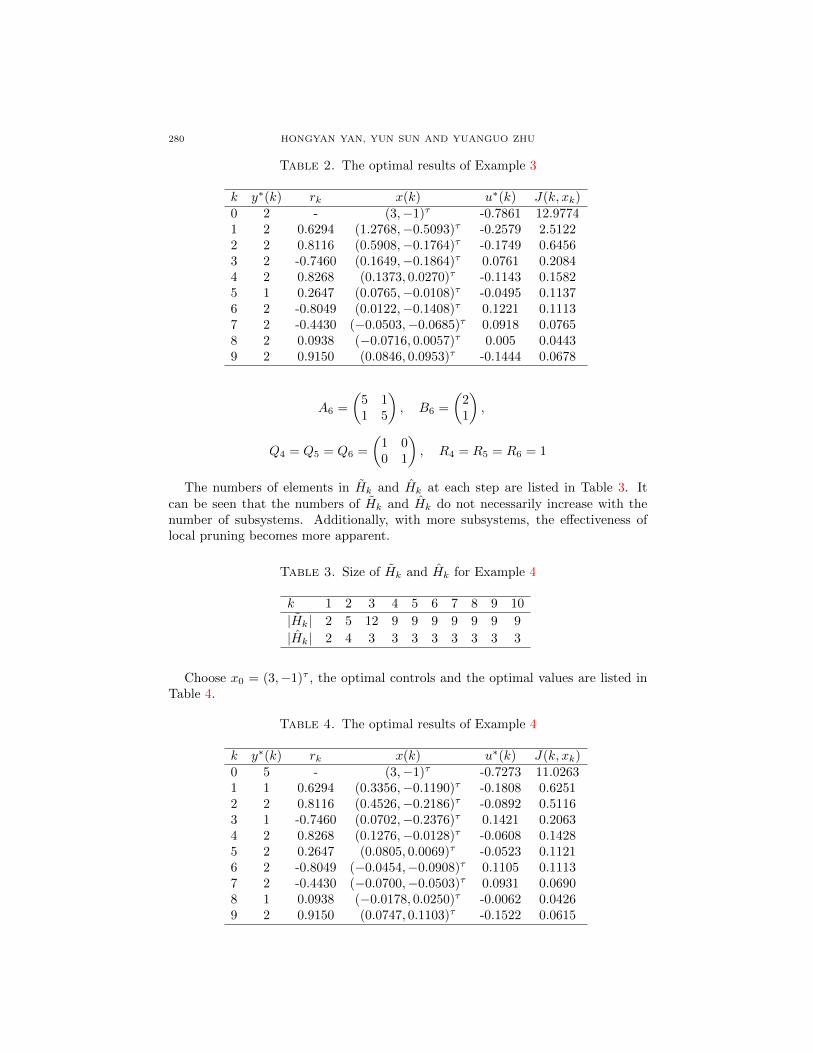
k y∗(k) rk x(k) u∗(k) J(k, xk)0 2 - (3,−1)τ -0.7861 12.97741 2 0.6294 (1.2768,−0.5093)τ -0.2579 2.51222 2 0.8116 (0.5908,−0.1764)τ -0.1749 0.64563 2 -0.7460 (0.1649,−0.1864)τ 0.0761 0.20844 2 0.8268 (0.1373, 0.0270)τ -0.1143 0.15825 1 0.2647 (0.0765,−0.0108)τ -0.0495 0.11376 2 -0.8049 (0.0122,−0.1408)τ 0.1221 0.11137 2 -0.4430 (−0.0503,−0.0685)τ 0.0918 0.07658 2 0.0938 (−0.0716, 0.0057)τ 0.005 0.04439 2 0.9150 (0.0846, 0.0953)τ -0.1444 0.0678
A6 =
(5 11 5
), B6 =
(21
),
Q4 = Q5 = Q6 =
(1 00 1
), R4 = R5 = R6 = 1
The numbers of elements in Hk and Hk at each step are listed in Table 3. Itcan be seen that the numbers of Hk and Hk do not necessarily increase with thenumber of subsystems. Additionally, with more subsystems, the effectiveness oflocal pruning becomes more apparent.
Table 3. Size of Hk and Hk for Example 4
k 1 2 3 4 5 6 7 8 9 10
|Hk| 2 5 12 9 9 9 9 9 9 9
|Hk| 2 4 3 3 3 3 3 3 3 3
Choose x0 = (3,−1)τ , the optimal controls and the optimal values are listed inTable 4.
Table 4. The optimal results of Example 4
k y∗(k) rk x(k) u∗(k) J(k, xk)0 5 - (3,−1)τ -0.7273 11.02631 1 0.6294 (0.3356,−0.1190)τ -0.1808 0.62512 2 0.8116 (0.4526,−0.2186)τ -0.0892 0.51163 1 -0.7460 (0.0702,−0.2376)τ 0.1421 0.20634 2 0.8268 (0.1276,−0.0128)τ -0.0608 0.14285 2 0.2647 (0.0805, 0.0069)τ -0.0523 0.11216 2 -0.8049 (−0.0454,−0.0908)τ 0.1105 0.11137 2 -0.4430 (−0.0700,−0.0503)τ 0.0931 0.06908 1 0.0938 (−0.0178, 0.0250)τ -0.0062 0.04269 2 0.9150 (0.0747, 0.1103)τ -0.1522 0.0615

A LINEAR-QUADRATIC CONTROL PROBLEM OF UDSS 281
7. Conclusions. A quadratic optimal control model for uncertain discrete-timeswitched linear systems whose subsystems are perturbed by uncertain factors hasbeen presented, together with a method to design a control strategy and a switchinglaw. The analytical solutions of the optimal objective function and the controlstrategy can be exactly characterized by Hk, whose size grows exponentially. Atwo-step pruning scheme is developed to prune out as many redundant matrices inHk as possible. The first step is a local pruning and the second step is a globalpruning. The examples validate the effectiveness of the method and show the factthat the greater the number of subsystems is, the better the effectiveness of thelocal pruning is.
Acknowledgments. This work is supported by the National Natural Science Foun-dation of China (No.61273009).
REFERENCES
[1] A. Bemporad, F. Borrelli and M. Morari, On the optimal control law for linear discretetime hybrid systems, Lecture Notes in Computer Science, Hybrid System: Computation and
Control , 2289 (2002), 222–292.
[2] S. C. Benga and R. A. Decarlo, Optimal control of switching systems, Automatica, 41 (2005),11–27.
[3] F. Borrelli, M. Baotic, A. Bemporad and M. Morari, Dynamic programming for contrained
optimal control of discrete-time linear hybrid systems, Automatica, 41 (2005), 1709–1721.[4] S. Boubakera, M. Djemaic, N. Manamannid and F. M’Sahlie, Active modes and switching in-
stants identification for linear switched systems based on discrete particle swarm optimization,
Applied Soft Computing, 14 (2014), 482–488.[5] H. V. Esteban, C. Patrizio, M. Richard and B. Franco, Discrete-time control for switched
positive systems with application to mitigating viral escape, International Journal of Robust
and Nonlinear Control , 21 (2011), 1093–1111.[6] Y. Gao, Uncertain models for single facility location problems on networks, Applied Mathe-
matical Modelling, 36 (2012), 2592–2599.[7] J. Gao and L. Duan, Linear-quadratic switching control with switching cost, Automatica, 48
(2012), 1138–1143.
[8] D. Kahneman and A. Tversky, Prospect theory: An analysis of decision under risk, Econo-metrica, 47 (1979), 263–292.
[9] H. W. J. Lee, K. L. Teo, V. Rehbock and L. S. Jennings, Control parametrization enhancing
technique for optimal discrete-valued control problems, Automatica, 35 (1999), 1401–1407.[10] F. Li, P. Shi, L. Wu, M. V. Basin and C. C. Lim, Quantized control design for cognitive
radio networks modeled as nonlinear semi-Markovian jump systems, IEEE Transactions on
Industrial Electronics, 62 (2015), 2330–2340.[11] B. Lincoln and A. Rantzer, Relaxing dynamic programming, IEEE Transactions on Auto-
matic Control , 51 (2006), 1249–1260.
[12] B. Liu, Why is there a need for uncertainty theory, Journal of Uncertain Systems, 6 (2012),3–10.
[13] B. Liu, Uncertainty Theory, 2nd edition, Springer-Verlag, Berlin, 2007.[14] B. Liu, Uncertainty Theory: A Branch of Mathematics for Modeling Human Uncertainty,
Springer-Verlag, Berlin, 2010.
[15] Y. Liu and M. Ha, Expected value of function of uncertain variables, Journal of UncertainSystems, 4 (2010), 181–186.
[16] C. Liu, Z. Gong and E. Feng, Modelling and optimal control for nonlinear multistage dynam-ical system of microbial fed-batch culture, Journal of Industrial and Management Optimiza-tion, 5 (2009), 835–850.
[17] R. Loxton, K. L. Teo, V. Rehbock and W. K. Ling, Optimal switching instants for a switched-
capacitor DC/DC power converter, Automatica, 45 (2009), 973–980.[18] K. L. Teo, C. J. Goh and K. H. Wong, A Unified Computational Approach to Optimal Control
Problems, Longman Scientific and Technical, New York, 1991.

282 HONGYAN YAN, YUN SUN AND YUANGUO ZHU
[19] C. Tomlin, G. J. Pappas, J. Lygeros, D. N. Godbole and S. Sastry, Hybrid control models ofnext generation air traffic management, Hybrid Systems IV , 1273 (1997), 378–404.
[20] L. Y. Wang, A. Beydoun, J. Sun and I. Kolmanasovsky, Optimal hybrid control with appli-
cation to automotive powertrain systems, Lecture Notes in Control and Information Science,222 (1997), 190–200.
[21] S. Woon, V. Rehbock and R. Loxton, Global optimization method for continuous-time sensorscheduling, Nonlinear Dynamic Systems Theory, 10 (2010), 175–188.
[22] L. Wu, D. Ho and C. Li, Sliding mode control of switched hybrid systems with stochastic
perturbation, Systems & Control Letters, 60 (2011), 531–539.[23] X. Xu and P. Antsaklis, Optimal control of switched systems based on parameterization of
the switching instants, IEEE Transactions on Automatic Control , 49 (2004), 2–16.
[24] H. Yan and Y. Zhu, Bang-bang control model for uncertain switched systems, Applied Math-ematical Modelling, 39 (2015), 2994–3002.
[25] H. Yan and Y. Zhu, Bang-bang control model with optimistic value criterion for uncertain
switched systems, Journal of Intelligent Manufacturing, (2015), 1–8.[26] W. Zhang, J. Hu and A. Abate, On the value function of the discrete-time switched lqr
problem, IEEE Transactions on Automatic Control , 54 (2009), 2669–2674.
[27] W. Zhang, J. Hu and J. Lian, Quadratic optimal control of switched linear stochastic systems,Systems & Control Letters, 59 (2010), 736–744.
[28] X. Zhang and X. Chen, A new uncertain programming model for project scheduling problem,Information: An International Interdisciplinary Journal, 15 (2012), 3901–3910.
[29] Y. Zhu, Uncertain optimal control with application to a portfolio selection model, Cybernetics
and Systems: An International Journal , 41 (2010), 535–547.[30] Y. Zhu, Functions of uncertain variables and uncertain programmin, Journal of Uncertain
Systems, 6 (2012), 278–288.
Received January 2015; 1st revision May 2015; final revision December 2015.
E-mail address: [email protected]
E-mail address: chinalsy [email protected]
E-mail address: [email protected]