A LINEAR MULTIFACTOR MODEL FOR REITS SELECTION USING ...ale44/MScWorkReport-LE.pdf · A LINEAR MULTIFACTOR MODEL FOR REITS SELECTION USING GRADIENT ... of the REIT on a public stock

A LINEAR MULTIFACTOR MODEL FOR REITS SELECTION USINGGRADIENT MAXIMIZATION

by

Anatole Le

DIRO

Universite de Montreal, Montreal

December 2006

A WORK REPORT SUBMITTED TOUNIVERSITE DE MONTREAL

IN PARTIAL FULFILLMENT OF THE REQUIREMENTS OF THE DEGREE OF

MASTER OFSCIENCE

Copyright c© 2006 by Anatole Le

Abstract

Investing in real estate can provide a good source of diversification as well as a hedge

against inflation. In this report, we describe a quantitative ranking model for portfolio

construction developed at Desjardins Global Asset Management for the market of Real

Estate Investment Trusts (REITs). The linear multifactor model uses eight signals and a

gradient maximization algorithm to compute the weights associated to each factor.

We used Java for developing the ranking system and implementthe gradient maximiza-

tion algorithm. We measured the performance of the model by backtesting it over data

ranging from 1995 to 2006. We simulated two long-only portfolios, the first one composed

of the highest ranked REITs by the model and the second one of the lowest ranked. We

restricted trading volume to 10% of a REIT’s daily volume andincluded a $0.05/share

transaction fee.

The simulations results were compared with the MSCI REIT index. The portfolio with

the highest ranked REITs outperformed the benchmark significantly by 7.5% on average

annually while the one with the lowest ranked REITs underperformed the index by 2.1%.

Annual volatility of the returns was higher for both portfolios (16.0% and 16.6%) than for

the benchmark (14.6%), but this increase is relatively small.

i

ii

Acknowledgments

The completion of this work would not have been possible without the help of many

people. I first would like to thank Robert Normand, my immediate boss and senior director

of the Quantitative Research & Management Group at Desjardins Global Asset Manage-

ment. My previous background was in mathematics and computer science, and Robert

helped me learn the required financial skills. I was also given lots of freedom to do re-

search and Robert provided guidance, many ideas and insights into the development of the

ranking model. I would also like to thank my colleague, Mariane Bastien, for her help with

learning about the REITs industry, for her constant search for new data, for her work with

the Compustat database and for the numerous discussions we had on the factors to include.

I also learned and received help from Dr Yoshua Bengio, who ischarge of the Master’s

program in Mathematical and Computational Finance at Universite de Montreal. In his

graduate course, Machine Learning Algorithms, I learned many statistical algorithms and

optimizations which I used in this work. Dr Bengio also provided ideas for improving the

effectiveness of the model and for optimizing the model parameters.

Throughout my graduate studies at Universite de Montreal, I was supported financially

with scholarships received from the Institut de Finance Mathematique de Montreal (IFM2)

and from the DIRO department at Universite de Montreal.

Finally, my last thoughts go to Cecile, who is always there to listen and advise when

needed, and whose love and support help me go through good anddifficult times.

iii

iv

Contents

Abstract i

Acknowledgments iii

Contents v

List of Figures vii

List of Tables ix

1 Introduction 1

1.1 What Are REITs . . . . . . . . . . . . . . . . . . . . . . . . . . . . . . . 1

1.2 Why Invest in REITs . . . . . . . . . . . . . . . . . . . . . . . . . . . . . 3

1.3 A Quantitative System for REITs Selection . . . . . . . . . . . .. . . . . 5

1.4 Report Organization . . . . . . . . . . . . . . . . . . . . . . . . . . . . . .5

2 Ranking Model 7

2.1 Overview . . . . . . . . . . . . . . . . . . . . . . . . . . . . . . . . . . . 7

2.2 Factors . . . . . . . . . . . . . . . . . . . . . . . . . . . . . . . . . . . . . 8

2.3 Gradient Maximization . . . . . . . . . . . . . . . . . . . . . . . . . . . .10

2.3.1 Algorithm . . . . . . . . . . . . . . . . . . . . . . . . . . . . . . . 10

2.3.2 Example . . . . . . . . . . . . . . . . . . . . . . . . . . . . . . . 12

2.4 Summary . . . . . . . . . . . . . . . . . . . . . . . . . . . . . . . . . . . 14

v

3 Experimental Framework 15

3.1 Data . . . . . . . . . . . . . . . . . . . . . . . . . . . . . . . . . . . . . . 15

3.2 Systems and Tools . . . . . . . . . . . . . . . . . . . . . . . . . . . . . . 16

3.3 Simulations Implementation . . . . . . . . . . . . . . . . . . . . . . .. . 16

3.3.1 Parameters . . . . . . . . . . . . . . . . . . . . . . . . . . . . . . 16

3.3.2 Rolling Window . . . . . . . . . . . . . . . . . . . . . . . . . . . 17

4 Simulations Results 19

4.1 Measurements . . . . . . . . . . . . . . . . . . . . . . . . . . . . . . . . . 19

4.2 Results . . . . . . . . . . . . . . . . . . . . . . . . . . . . . . . . . . . . . 20

5 Conclusions and Future Work 27

5.1 Conclusions . . . . . . . . . . . . . . . . . . . . . . . . . . . . . . . . . . 27

5.2 Future Work . . . . . . . . . . . . . . . . . . . . . . . . . . . . . . . . . . 28

5.2.1 Rebalancing . . . . . . . . . . . . . . . . . . . . . . . . . . . . . . 28

5.2.2 Classification and Regression Trees . . . . . . . . . . . . . . .. . 28

5.2.3 Combining Models . . . . . . . . . . . . . . . . . . . . . . . . . . 29

Appendices

A Gradient Maximization Computed Weights 31

B Simulations Monthly Returns 35

Bibliography 41

vi

List of Figures

1.1 Daily Dollar Volume (millions) of NAREIT Index . . . . . . . .. . . . . . 2

1.2 Sector Capitalization of NAREIT Index . . . . . . . . . . . . . . .. . . . 2

1.3 REITs Correlation with Various Asset Classes . . . . . . . . .. . . . . . . 3

1.4 REITs Dividend Yield vs. 10-Year Treasury Bonds Yield . .. . . . . . . . 4

1.5 Annual Return of Various Asset Classes . . . . . . . . . . . . . . .. . . . 4

1.6 Annual Volatility of Various Asset Classes . . . . . . . . . . .. . . . . . . 4

2.1 Ranking Model for Portfolio Selection . . . . . . . . . . . . . . .. . . . . 9

2.2 Example of Determining the Gradient . . . . . . . . . . . . . . . . .. . . 12

2.3 Illustration of the Gradient Maximization with Two Factors . . . . . . . . . 13

4.1 Cumulative Returns of Simulated Portfolios and Index . .. . . . . . . . . 23

4.2 Annual Excess Return of Simulated Portfolios over Index. . . . . . . . . . 25

4.3 Annual Tracking Error of Simulated Portfolios . . . . . . . .. . . . . . . 26

vii

viii

List of Tables

4.1 Simulations Results . . . . . . . . . . . . . . . . . . . . . . . . . . . . . .22

4.2 Excess Return Measurements . . . . . . . . . . . . . . . . . . . . . . . .. 24

A.1 Weights Computed for Highest-Ranked Strategy . . . . . . . .. . . . . . . 32

A.2 Weights Computed for Lowest-Ranked Strategy . . . . . . . . .. . . . . . 33

B.1 Monthly Return for 1998 . . . . . . . . . . . . . . . . . . . . . . . . . . . 35

B.2 Monthly Return for 1999 and 2000 . . . . . . . . . . . . . . . . . . . . .. 36




ix

Chapter 1

Introduction

1.1 What Are REITs

A Real Estate Investment Trust (REIT) is a corporation or trust that owns, manages, ac-

quires, develops, and finances income-producing real estate. As a publicly traded company,

a REIT allows smaller investors to invest in commercial realestate by purchasing shares

of the REIT on a public stock exchange [REI04], and improves liquidity over investing

directly in real estate. Various characteristics of REITs include that a REIT must pay 90%

of its taxable income through dividend payments, 75% of its assets must be invested in real

estate or mortgage loans, and 75% of gross income must be derived from rents, interests

on mortgages from real estate property, or gains on sales of real estate assets. Also, a REIT

must have at least one hundred shareholders with the five largest owning less than 50% of

the total number of outstanding shares.

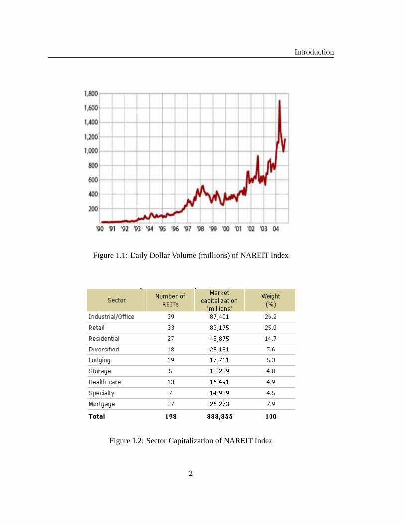
REITs have grown dramatically as an asset class over the lastdecade as can be seen

from Figure 1.1 which shows the daily transaction volume (inmillions) for the NAREIT

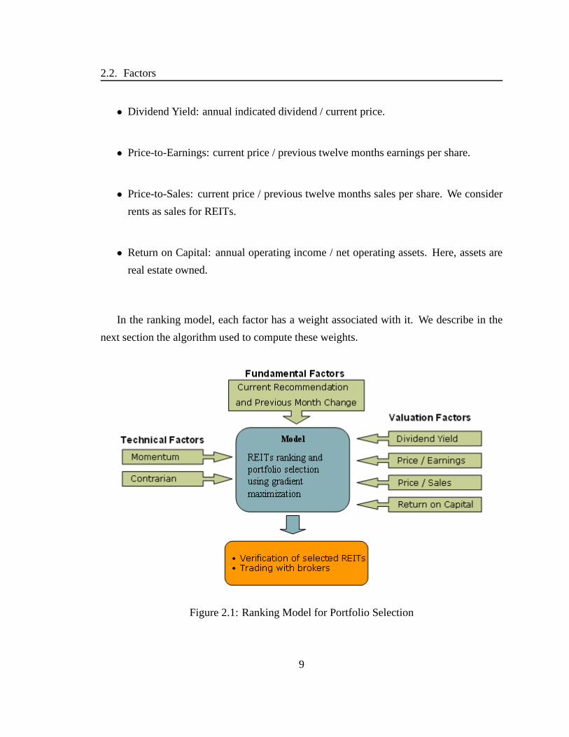
index. Figure 1.2 provides a break-down of the sector capitalization within the NAREIT

index as of September 2005.

1

Introduction

Figure 1.1: Daily Dollar Volume (millions) of NAREIT Index

Figure 1.2: Sector Capitalization of NAREIT Index

2

1.2. Why Invest in REITs

1.2 Why Invest in REITs

An advantage of including REITs in a portfolio is that it can reduce overall portfolio risk

through diversification since real estate has had in the pasta low correlation with other asset

classes. Figure 1.3 shows the correlation of the NAREIT index with short-term and long-

term bonds as well as large-cap and small-cap indices (Russell 1000 and Russell 2000).

Figure 1.3: REITs Correlation with Various Asset Classes

Another advantage of investing in REITs is that it can provide a hedge against inflation

as rental increases provide protection from increase in prices, and delivering strong cash

flows regularly through dividend payments [FSH05]. We see inFigure 1.4 that the REITs

dividend yield has been higher than the 10-year Treasury bond yield since 1999.

Over the past 7 years, REITs produced a higher total return than the major stock mar-

ket indices as well as long-term bonds while exhibiting smaller volatility than the Russell

indices (see Figures 1.5 and 1.6).

3

Introduction

Figure 1.4: REITs Dividend Yield vs. 10-Year Treasury BondsYield

Figure 1.5: Annual Return of Various Asset Classes

Figure 1.6: Annual Volatility of Various Asset Classes

4

1.3. A Quantitative System for REITs Selection

1.3 A Quantitative System for REITs Selection

The benefits of investing in real estate have led the Quantitative Group at Desjardins Global

Asset Management (DGAM) to pursue a project of developing a quantitative system for

REITs selection as part of a global portfolio.

We developed a ranking system for REITs based on a multifactor model. The model

ranks each REIT by using a linear combination of eight factors. A gradient maximization

algorithm is used to compute the weights for the model. We also implemented various

optimizations for the model parameters such as the number ofREITs to carry in the portfo-

lio and the maximum holding rank for a REIT. The latter provides a rank threshold under

which a REIT is sold. We performed various experiments to validate and measure the

performance of the model over data ranging from 1995 to 2006.While taking into con-

sideration transaction costs and liquidity, we simulated long-only portfolios composed of

the highest ranked and of the lowest ranked REITs by the model. The backtests results

produced for the first portfolio annual excess return averaging 7.5%. For the second simu-

lated portfolio, it underperformed the MSCI REIT index by 2.1% on average annually. A

production version of this model is currently in place and used for REITs selection in a real

portfolio.

1.4 Report Organization

The remainder of this report is organized as follows. The next chapter describes the REITs

ranking system. We first provide an overview of the model, then we discuss the selected

factors used by the model, and finally we describe the implementation of the gradient max-

imization algorithm used to compute the weights associatedto each factor. In Chapter 3,

we specify the data and the environment in which we conductedthe experiments, and give

details on the implementation of the simulations. In Chapter 4, we discuss the results ob-

tained and compare them with the MSCI REIT index. We concludewith Chapter 5 and

suggest potential areas for future work.

5

Introduction

6

Chapter 2

Ranking Model

2.1 Overview

The ranking system is based on a multifactor model where eachREIT is assigned a score

based on a combination of several factors. The scores are sorted in decreasing order, giving

a ranking from the strongest REITs to the weakest ones according to the model. The score

of a REIT is a function of the selected factors or signals. Foreach factor, its value is

computed for every REIT. The values are then sorted in decreasing order and divided into

deciles. REITs in the top decile get a score of 10 for that particular factor, those in the

second best decile have a value of 9, and so on until the bottomdecile where REITs are

assigned a score of 1. If some data is missing and as a result the value of a factor cannot be

computed for a REIT, we assign it a score of 3. For example, if we consider the dividend

yield factor, the top 10% of REITs with the highest dividend yield will have a score of

10 while the bottom 10% will get a score of 1. If for any reason we cannot compute the

dividend yield of a REIT, we will assign it a value of 3. Finally, the ranking score of a

REIT is a linear function of the individual factors scores. The following equation gives the

score of REITr j wherewi denotes the weight associated with factorfi .

score(r j) =n

∑i=1

wi fi(r j) (2.1)

7

Ranking Model

The weightswi are computed using a gradient maximization algorithm whichwe de-

scribe in Section 2.3. We note that since the weights sum to 1 and that the score for each

factor is in the range of 1 to 10, the minimum and maximum ranking scores are 1 and 10

respectively for a REIT.

2.2 Factors

For the n-factor ranking model, we selected eight market factors that can be grouped in

three categories: technical, valuation (accounting ratios) and fundamental (analysts recom-

mendations). We used two technical signals: 6-month price momentum and 5-day price

contrarian. We used four standard accounting ratios: dividend yield, price-to-earnings,

price-to-sales and return on capital. Finally, we used two analysts signals: current rec-

ommendation (buy, hold or sell) and recommendation change from the previous month

(upgrade, downgrade or no change) from Green Street Advisors, a research and brokerage

firm dedicated to the REITs’ market. Recommendations from Green Street are made based

on their proprietary calculation of net asset value (NAV) asa relative valuation measure for

REITs in their respective sector. We note that for the analysts signals, we cannot split them

into deciles since there are only three possible values for the current recommendation and

recommendation change factors. We thus assign a value of 10,5 and 1 respectively for buy,

hold and sell recommendations. We do the same for upgrade, nochange and downgrade

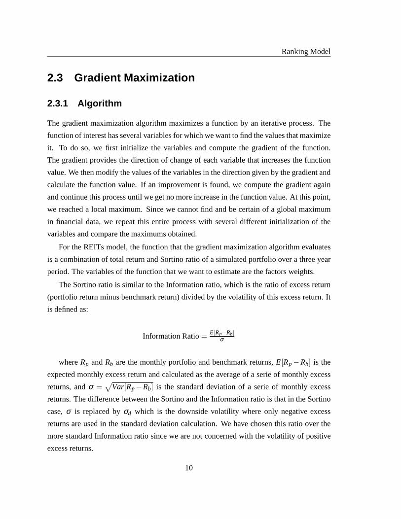
for the recommendation change factor. In Figure 2.1, we showa high-level overview of the

model.

Below, we provide details of the calculation of the technical signals and accounting

ratios used by the model.

• Price momentum:(Pt−1+Divt−7,t−1)/Pt−7 wherePt−1 is the price 1-month prior to

time t andDivt−7,t−1 is the total dividend from montht −7 to montht −1. Interme-

diate term positive momentum is viewed as favorable.

• Price contrarian:(Pt−1 + Divt−6,t−1)/Pt−6 wherePt−1 is the price 1-day prior and

Divt−6,t−1 is the dividend from dayt −6 to t −1. Short-term reversal in the trend is

viewed as favorable.

8

2.2. Factors

• Dividend Yield: annual indicated dividend / current price.

• Price-to-Earnings: current price / previous twelve monthsearnings per share.

• Price-to-Sales: current price / previous twelve months sales per share. We consider

rents as sales for REITs.

• Return on Capital: annual operating income / net operating assets. Here, assets are

real estate owned.

In the ranking model, each factor has a weight associated with it. We describe in the

next section the algorithm used to compute these weights.

Figure 2.1: Ranking Model for Portfolio Selection

9

Ranking Model

2.3 Gradient Maximization

2.3.1 Algorithm

The gradient maximization algorithm maximizes a function by an iterative process. The

function of interest has several variables for which we wantto find the values that maximize

it. To do so, we first initialize the variables and compute thegradient of the function.

The gradient provides the direction of change of each variable that increases the function

value. We then modify the values of the variables in the direction given by the gradient and

calculate the function value. If an improvement is found, wecompute the gradient again

and continue this process until we get no more increase in thefunction value. At this point,

we reached a local maximum. Since we cannot find and be certainof a global maximum

in financial data, we repeat this entire process with severaldifferent initialization of the

variables and compare the maximums obtained.

For the REITs model, the function that the gradient maximization algorithm evaluates

is a combination of total return and Sortino ratio of a simulated portfolio over a three year

period. The variables of the function that we want to estimate are the factors weights.

The Sortino ratio is similar to the Information ratio, whichis the ratio of excess return

(portfolio return minus benchmark return) divided by the volatility of this excess return. It

is defined as:

Information Ratio= E[Rp−Rb]σ

whereRp andRb are the monthly portfolio and benchmark returns,E[Rp−Rb] is the

expected monthly excess return and calculated as the average of a serie of monthly excess

returns, andσ =√

Var[Rp−Rb] is the standard deviation of a serie of monthly excess

returns. The difference between the Sortino and the Information ratio is that in the Sortino

case,σ is replaced byσd which is the downside volatility where only negative excess

returns are used in the standard deviation calculation. We have chosen this ratio over the

more standard Information ratio since we are not concerned with the volatility of positive

excess returns.

10

2.3. Gradient Maximization

The gradient maximization algorithm has been implemented as described by Brush and

Schock [BS95]. We highlight the six steps in this process below:

(I) Initialize weights randomly.

(II) Simulate portfolios composed of the highest ranked REITs for all combinations

of weights adjusted by +/- 20% over three years of daily data.

(III) Compute total return and Sortino ratio for each simulation.

(IV) Modify the weights in the direction given by the best simulated portfolio in

Step III, and perform simulations in this direction until a local maximum is

reached.

(V) Repeat Steps (II), (III) and (IV) until no improvement isfound.

(VI) Repeat the entire process from Step (I) with different initial weights.

It should be noted that the gradient computation is done by Steps II and III, i.e. we

adjust the weights in every direction, we simulate portfolios using these weights, and we

compute portfolio return and Sortino ratio. The direction of weights adjustments (the gradi-

ent) can then be found by choosing the portfolio that best combines total return and Sortino

ratio (the criteria to maximize).

11

Ranking Model

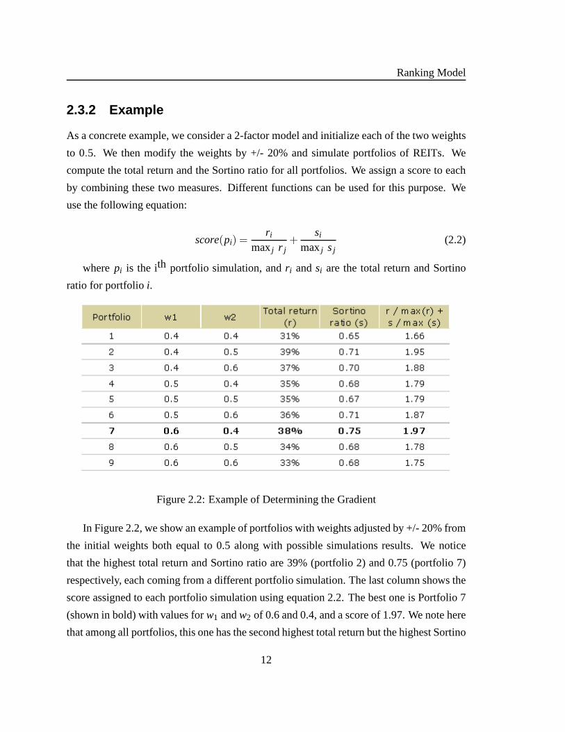
2.3.2 Example

As a concrete example, we consider a 2-factor model and initialize each of the two weights

to 0.5. We then modify the weights by +/- 20% and simulate portfolios of REITs. We

compute the total return and the Sortino ratio for all portfolios. We assign a score to each

by combining these two measures. Different functions can beused for this purpose. We

use the following equation:

score(pi) =r i

maxj r j+

si

maxj sj(2.2)

wherepi is the ith portfolio simulation, andr i andsi are the total return and Sortino

ratio for portfolioi.

Figure 2.2: Example of Determining the Gradient

In Figure 2.2, we show an example of portfolios with weights adjusted by +/- 20% from

the initial weights both equal to 0.5 along with possible simulations results. We notice

that the highest total return and Sortino ratio are 39% (portfolio 2) and 0.75 (portfolio 7)

respectively, each coming from a different portfolio simulation. The last column shows the

score assigned to each portfolio simulation using equation2.2. The best one is Portfolio 7

(shown in bold) with values forw1 andw2 of 0.6 and 0.4, and a score of 1.97. We note here

that among all portfolios, this one has the second highest total return but the highest Sortino

12

2.3. Gradient Maximization

ratio. Thus, the direction of the gradient for weightw1 is positive (since 0.6 is higher than

the initial 0.5 value) and forw2 it is negative (since 0.4 is lower than 0.5).

Figure 2.3 (from [BS95]) shows the gradient maximization iterative process for a 2-

factor model (two weights to estimate). Point 1 is the starting point where weights are

initialized (Step I). The black dots surrounding Point 1 in the figure correspond to the

modification of the weights (Step II) to find the direction of highest improvement (Step

III). We see in the picture that this direction is pointing towards Point 2. Weights are

adjusted in this direction (Step IV) until a local maximum isreached (Point 2). Steps II,

III and IV are performed until Point 3 is reached, and again until Point 4. At that point,

modifying the weights does not improve the solution.

Figure 2.3: Illustration of the Gradient Maximization withTwo Factors

13

Ranking Model

2.4 Summary

In summary, the ranking model is a 4-step quantitative process:

(I) For each of the eight factors, rank REITs based on the values of the factor.

(II) For every factor, divide the ranking into deciles and assign them a score of 1

(bottom decile) to 10 (top decile).

(III) Compute weights for each factor using the gradient maximization algorithm

described in Section 2.3.

(IV) Compute the total score for each REIT using equation 2.1.

In this chapter, we described the ranking system used for selecting REITs in a portfolio.

In the next chapter, we discuss the experimental framework in which we ran simulations to

evaluate the performance of the model.

14

Chapter 3

Experimental Framework

In this chapter, we describe the environment in which we conducted experiments to

evaluate the performance of the ranking model. The next section describes the data that we

used. Section 3.2 specifies the systems and tools used for thedevelopment of the model and

for the simulations. Finally, in Section 3.3, we give details of the simulations, including

the various parameters used by the model and the implementation of the train/test rolling

window employed to evaluate its performance.

3.1 Data

For our experiments, we used data ranging from January 1995 to June 2006 from the S&P

Compustat database, including daily prices, dividend dataat the ex-date, and quarterly fun-

damental data to compute price-to-earnings, price-to-sales, dividend yield and return on

capital ratios. For the quarterly fundamentals, we used thePoint-in-Time package in Com-

pustat which shows the data that was available in the database historically at a given point in

time. For example, if a REIT had its earnings per share for thelast quarter of 1999 restated

in 2001, then in our simulations we used the unrestated valuein 2000 but the restated one

in 2001. Hence, the Point-in-Time package keeps track of financial restatements making

backtests results more reliable.

We considered for our sample the set of REITs covered by GreenStreet Advisors, in-

cluding those that do not exist anymore, have merged, or stopped being followed. To limit

15


the effect of survivorship bias, we included every REIT thatreceived monthly recommen-

dations between 1995 and 2006 by Green Street. This gave us approximately 150 REITs

for the entire period, of which about ten were eliminated dueto unavailability of prices or

quarterly data. We note that typically, for any given month,there were around 60 to 70

REITs covered by Green Street.

3.2 Systems and Tools

The development of the model as well as the simulations have been made in the Java pro-

gramming language using JDK 1.5.0 Update 6 within the Cygwinenvironment. The ma-

chine used for the implementation and for running the experiments was an Intel Pentium 4,

2.8 GHz system with 2 GBs of RAM running Microsoft Windows XP Professional Version

2002 Service Pack 2.

3.3 Simulations Implementation

3.3.1 Parameters

In Section 2.3, we described how the gradient maximization algorithm computes the weights

associated to each factor. In our simulations, two additional parameters, which we called

PF SIZEandMAX HOLD RANK, also needed to be optimized. The first one specified

the number of REITs to buy when there was cash available in theportfolio. For example,

if after optimizationPF SIZEwas set to 12, then every day if the portfolio had money

available then the top 12 ranked REITs by the model were purchased with equal weights.

For the second parameter, it provided the maximum rank of a REIT to stay in the portfolio.

For example, if the maximum rank was 30, then whenever the rank of a REIT contained in

the portfolio fell below 30, we got rid of it. We added these two parameters to the factors

weights to be optimized as part of the gradient maximizationalgorithm.

In our simulations, we allocated an initial capital of 10 millions dollars for the portfolio.

The simulations were performed daily and whenever there wasmoney available in the port-

folio, the highestPF SIZEranked REITs by the model were purchased (equal-weighted).

16

3.3. Simulations Implementation

If a REIT held in the portfolio had a rank lower thanMAX HOLD RANK, we sold it.

When establishing a position for a REIT, we limited the maximum number of shares that

we bought or sold to 10% of the REIT’s daily volume. We included a $0.05 fee for the cost

of each share transaction, and used the average of the daily high, low and close price for

the transaction price.

3.3.2 Rolling Window

We implemented the backtesting of the ranking system by using the rolling train/test win-

dow model typically used in learning algorithms and described in [Lev95]. We performed

sequential validation of the model by training the gradientmaximization over three years

of continuous data, and then evaluated the computed weightson the subsequent six months

of data. The gradient maximization algorithm was thus invoked every six months. Since

our data is from January 1995 to June 2006, the simulations ofthe portfolios started in

January 1998 using computed weights by the gradient maximization on data from January

1995 until December 1997. The performance of the portfolioswas then measured using

these weights on six months of out-of-sample data from January 1998 to June 1998. In

July 1998, the gradient maximization algorithm was invokedagain, and the data for train-

ing and testing were moved accordingly, i.e. the weights were recomputed using data from

July 1995 until June 1998 and the performance was evaluated using the new computed

weights on out-of-sample data from July 1998 to December 1998. The window of data for

training and testing was moved forward this way until the endof the simulations in June

2006. We note that the signals were calculated daily. Hence,the model ranked REITs on a

daily basis, and positions were evaluated and rebalanced accordingly.

We simulated two long-only portfolios: the first one composed of the highest ranked

REITs by the model and the second one of the lowest. We used thegradient maximization

algorithm to compute weights for each. Invoking the gradient maximization for selecting

low performing REITs is the opposite of for high performing REITs, i.e. instead of maxi-

mizing total return and Sortino ratio we minimize it. In Appendix A, we show the weights

computed every six months for both simulations.

17


18

Chapter 4

Simulations Results

In the previous chapter, we discussed the experimental framework and the implementa-

tion of the highest- and lowest-ranked REITs simulations using the gradient maximization

algorithm. In the following sections, we present the performance measurements of the

simulated portfolios.

4.1 Measurements

The performance measurements of the ranking model start in January 1998 and end in June

2006. We list and provide details of the various measurements for the simulations results

contained in Tables 4.1 and 4.2.

• Position Size (µ): daily average number of REITs held in portfolio.

• Position Cash (µ andσ ): daily average and standard deviation of cash position as a

percentage of total portfolio value.

• Monthly Turnover (µ andσ ): A measurement of portfolio trading activity. A high

turnover value means assets are bought and sold frequently and thus high transaction

costs are incurred. The value for a given month is calculatedby dividing the monthly

total dollar value of purchases or sales (whichever is less)by the average total value

of the portfolio in the month.

19

Simulations Results

• Monthly Return (µ): average monthly return of portfolio.

• Yearly Return: portfolio return in a given year.

• Total Return: portfolio return from the simulation start date until the end date.

• Annual Volatility: standard deviation of the serie of portfolio monthly returns multi-

plied by√

12.

• Maximum Drawdown: largest percentage loss from a peak in portfolio value to a

bottom.

• Recovery Date: date at which the portfolio value recovered from the maximum draw-

down.

• Excess Return (µ andσ ): average and standard deviation of the serie of monthly ex-

cess returns over the MSCI REIT index. Excess return for a given month is calculated

as the portfolio return for that month minus the index return.

• Months Positive: number of months where the excess return ispositive.

• Tracking Error: standard deviation of the serie of monthly excess returns multiplied

by√

12.

• Information Ratio: average of the serie of monthly excess returns divided by the

standard deviation of the serie.

• Sortino Ratio: same as the Information ratio except that only negative excess returns

are taken into account when computing the standard deviation of the serie of excess

returns.

4.2 Results

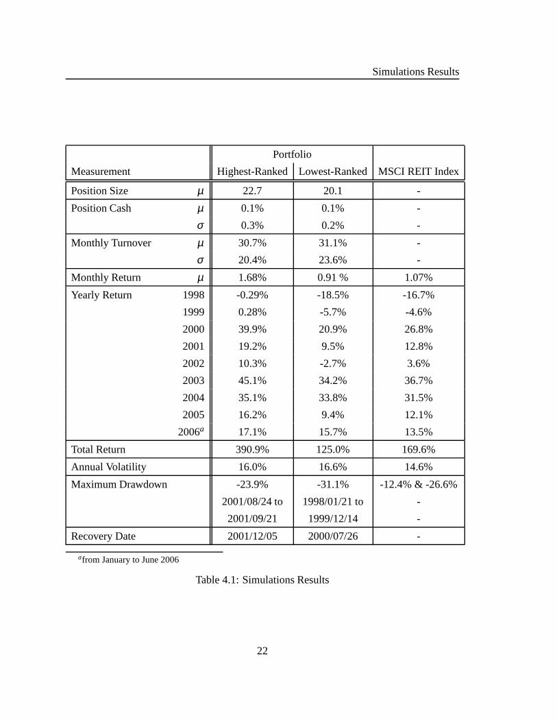
The results of the ranking model simulations are shown in Table 4.1. It should be noted

that the yearly return for 2006 only includes the first six months. The first row of Table 4.1

20

4.2. Results

shows that the average number of REITs held daily in the highest- and lowest-ranked port-

folios is about the same. Similarly for the daily cash position for both models which had

only 0.1% on average, and hence our restriction of limiting transaction volume to 10% of

the daily volume did not cause liquidity issues. For both strategies, the turnover was around

31%, a large but not excessive value. This means that each portfolio was rolled over ap-

proximately 3 1/2 times per year. The monthly return for the highest-ranked portfolio was

1.68%, much higher than for the benchmark (1.07%). For the lowest-ranked simulation,

the monthly return was 0.91%, which is below the index. We note that if we wanted to be

market neutral, this difference would not be significant enough to short the lowest-ranked

portfolio since taking into account the repo rate (the cost of borrowing shares for shorting),

the performance would approximately be the same as the indexbut with more risks (see

discussion on volatility below).

In the middle rows, we see the yearly returns from 1998 to 2006(only the first six

months are included in 2006). In every year, the highest-ranked simulation outperformed

both the lowest-ranked portfolio and the benchmark. For thelowest-ranked portfolio, it

underperformed the benchmark each year except for 2004 and 2006. The highest-ranked

portfolio thus outperformed much more the benchmark and more consistently than the

lowest-ranked portfolio underperformed it. The total returns for both simulations as well

as for the index were 390.9%, 125.0% and 169.6% respectively, with annual volatility of

16.0%, 16.6% and 14.6%. Although the volatility of the benchmark returns was smaller

than the ones for the simulations, the difference is not significant compared with the excess

returns generated by the highest-ranked portfolio. However, this increase in risks may not

justify the shorting of the lowest-ranked portfolio given its small underperformance.

The last two rows of Table 4.1 show the maximum drawdown and recovery date for the

simulations. For the first portfolio, the largest decrease in value from any given point was

-23.9% while the index dropped by -12.4% for the same period.It then took 2 1/2 months

for the portfolio to return to that peak. For the second portfolio, the maximum drawdown

was -31.1% (-26.6% for the benchmark) but it took more than seven months to recover

from this drop.

21

Simulations Results

Portfolio

Measurement Highest-Ranked Lowest-Ranked MSCI REIT Index

Position Size µ 22.7 20.1 -

Position Cash µ 0.1% 0.1% -

σ 0.3% 0.2% -

Monthly Turnover µ 30.7% 31.1% -

σ 20.4% 23.6% -

Monthly Return µ 1.68% 0.91 % 1.07%

Yearly Return 1998 -0.29% -18.5% -16.7%

1999 0.28% -5.7% -4.6%

2000 39.9% 20.9% 26.8%

2001 19.2% 9.5% 12.8%

2002 10.3% -2.7% 3.6%

2003 45.1% 34.2% 36.7%

2004 35.1% 33.8% 31.5%

2005 16.2% 9.4% 12.1%

2006a 17.1% 15.7% 13.5%

Total Return 390.9% 125.0% 169.6%

Annual Volatility 16.0% 16.6% 14.6%

Maximum Drawdown -23.9% -31.1% -12.4% & -26.6%

2001/08/24 to 1998/01/21 to -

2001/09/21 1999/12/14 -

Recovery Date 2001/12/05 2000/07/26 -

afrom January to June 2006

Table 4.1: Simulations Results

22

4.2. Results

We show cumulative total returns of the simulated portfolios and of the MSCI REIT

index (the benchmark) in Figure 4.1 for a $100 investment at the beginning of the period

in January 1998 until June 2006. We see in the figure that the highest-ranked strategy

outperformed the lowest-ranked portfolio and the benchmark significantly for the entire

period. The lowest-ranked simulation underperformed the index modestly, and hence we

do not recommend it as a shorting strategy since a cost of 1.0-1.5% annually would be

incurred for borrowing shares.

Figure 4.1: Cumulative Returns of Simulated Portfolios andIndex

23

Simulations Results

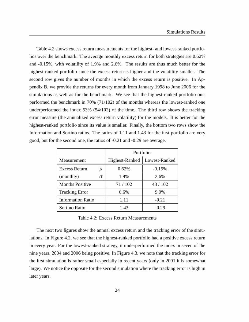
Table 4.2 shows excess return measurements for the highest-and lowest-ranked portfo-

lios over the benchmark. The average monthly excess return for both strategies are 0.62%

and -0.15%, with volatility of 1.9% and 2.6%. The results arethus much better for the

highest-ranked portfolio since the excess return is higherand the volatility smaller. The

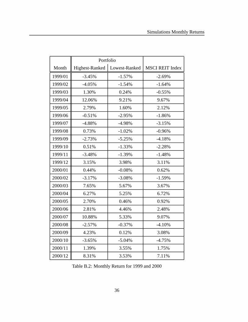
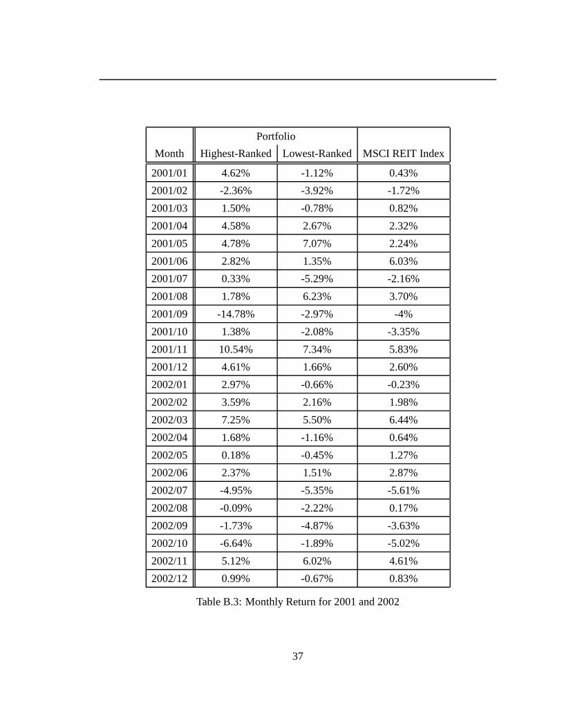
second row gives the number of months in which the excess return is positive. In Ap-

pendix B, we provide the returns for every month from January1998 to June 2006 for the

simulations as well as for the benchmark. We see that the highest-ranked portfolio out-

performed the benchmark in 70% (71/102) of the months whereas the lowest-ranked one

underperformed the index 53% (54/102) of the time. The thirdrow shows the tracking

error measure (the annualized excess return volatility) for the models. It is better for the

highest-ranked portfolio since its value is smaller. Finally, the bottom two rows show the

Information and Sortino ratios. The ratios of 1.11 and 1.43 for the first portfolio are very

good, but for the second one, the ratios of -0.21 and -0.29 areaverage.

Portfolio

Measurement Highest-Ranked Lowest-Ranked

Excess Return µ 0.62% -0.15%

(monthly) σ 1.9% 2.6%

Months Positive 71 / 102 48 / 102

Tracking Error 6.6% 9.0%

Information Ratio 1.11 -0.21

Sortino Ratio 1.43 -0.29

Table 4.2: Excess Return Measurements

The next two figures show the annual excess return and the tracking error of the simu-

lations. In Figure 4.2, we see that the highest-ranked portfolio had a positive excess return

in every year. For the lowest-ranked strategy, it underperformed the index in seven of the

nine years, 2004 and 2006 being positive. In Figure 4.3, we note that the tracking error for

the first simulation is rather small especially in recent years (only in 2001 it is somewhat

large). We notice the opposite for the second simulation where the tracking error is high in

later years.

24

4.2. Results

Figure 4.2: Annual Excess Return of Simulated Portfolios over Index

25

Simulations Results

Figure 4.3: Annual Tracking Error of Simulated Portfolios

26

Chapter 5

Conclusions and Future Work

5.1 Conclusions

In this report, we first gave a description of REITs and discussed several advantages of

investing in them. We then described the development of a quantitative system for REITs

selection based on a multifactor model. Eight factors were chosen for the model: price

momentum, price contrarian, current analyst recommendation, change in recommendation

from the previous month, dividend yield, price-to-earnings, price-to-sales and return on

capital. The model combined these signals linearly, and used a gradient maximization

algorithm to compute the weights associated to each factor.

We conducted experiments by backtesting the model using a rolling train/test window

over data ranging from 1995 to 2006. We performed simulations of portfolios composed

of the highest- and lowest-ranked REITs by the model. We limited transaction volume to

10% of a REIT’s daily volume and assumed a fee of $0.05 for eachshare transacted.

Finally, we measured the performance of the simulations andcompared the results with

the MSCI REIT index. The results of the simulations show thatthe highest-ranked strategy

outperformed the benchmark significantly and had returns inexcess of 7.5% annually on

average. In every year from 1998 to 2006, the excess return was positive while the annual

volatility was only 1.4% higher (16.0% versus 14.6% for the benchmark). For the lowest-

ranked simulation, the portfolio underperformed the indexby 2.1% on average annually

with a 2.0% increase in volatility (16.6%).

27


5.2 Future Work

5.2.1 Rebalancing

In our simulations, when a set of REITs was selected to be purchased, each one of them

was allocated the same amount of money, i.e. positions were equal-weighted. In contrast,

different trading methods could be explored. An interesting alternative would be the anticor

algorithm presented by Borodin, El-Yaniv and Gogan [BEYG04], which on the premise

that constant rebalancing can improve performance, have developed a technique that takes

advantage of predictable correlation between pairs of stocks.

5.2.2 Classification and Regression Trees

Classification and Regression Trees (CART) is a non-parametric method that classifies ob-

servations into categories, or in the continuous case into regression trees. CART is modeled

in the form of binary trees that represent decision rules. Each internal node in the binary

tree split sample data into two nodes based on the variable value associated with that node

(in this case the associated factor’s value). As such, CART is also known as binary recursive

partitioning since parent nodes are always split into exactly two child nodes and recursive

because the process can be repeated by treating each child node as a parent [whies]. This

hierarchical representation results in data clusters starting from the root node with the entire

learning data and end with small group of homogeneous observations [And05].

It would be interesting to experiment with a CART model sinceit has been a proven

robust data-mining and data-analysis tool used in the past and capable of discovering im-

portant patterns and relationships in highly complex data.CART’s set of decision rules

could also provide intuition in the relationships between the different factors affecting the

performance of REITs, and consequently provide a high degree of result’s interpretability.

28

5.2. Future Work

5.2.3 Combining Models

It is known that combining various predictors can improve upon using predictors individu-

ally. Thus, the ranking model described in this report couldbe used in conjunction with a

CART model. An investigation of committee and bagging techniques [KV95,Bre94] could

be performed to see whether factors affecting REITs performance could be generalized.

29


30

Appendix A

Gradient Maximization Computed Weights

In the following two tables, we show the weights that were computed every six months

by the gradient maximization algorithm for the highest- andlowest-ranked portfolio simu-

lations. We note that the weights in a row may not always sum to1 because of rounding to

the second decimal. In the tables, the corresponding factors are:

• F1: Contrarian

• F2: Current Green Street Recommendation

• F3: Recommendation Change from Previous Month by Green Street

• F4: Momentum

• F5: Dividend Yield

• F6: Price-to-Earnings

• F7: Price-to-Sales

• F8: Return on Capital

31


Factor

Date F1 F2 F3 F4 F5 F6 F7 F8

1998/01/01 0.23 0.05 0.3 0.22 0.02 0.03 0.05 0.09

1998/07/01 0.15 0.14 0.19 0.23 0.04 0.04 0.12 0.09

1999/01/01 0.24 0.07 0.35 0.16 0.02 0.05 0.06 0.06

1999/07/01 0.23 0.27 0.29 0.06 0.04 0.02 0.07 0.01

2000/01/01 0.3 0.08 0.24 0.16 0.03 0.05 0.08 0.06

2000/07/01 0.14 0.18 0.25 0.08 0.05 0.06 0.18 0.05

2001/01/01 0.12 0.18 0.25 0.1 0.04 0.06 0.17 0.07

2001/07/01 0.22 0.05 0.37 0.07 0.08 0.09 0.1 0.03

2002/01/01 0.13 0.09 0.15 0.17 0.12 0.13 0.14 0.07

2002/07/01 0.15 0.11 0.15 0.23 0.12 0.08 0.08 0.09

2003/01/01 0.13 0.13 0.21 0.16 0.11 0.08 0.05 0.12

2003/07/01 0.12 0.14 0.13 0.14 0.09 0.14 0.11 0.14

2004/01/01 0.11 0.1 0.13 0.13 0.14 0.12 0.06 0.2

2004/07/01 0.12 0.14 0.14 0.14 0.09 0.11 0.08 0.17

2005/01/01 0.17 0.11 0.2 0.09 0.07 0.14 0.05 0.17

2005/07/01 0.19 0.11 0.2 0.12 0.05 0.09 0.08 0.16

2006/01/01 0.12 0.2 0.21 0.1 0.06 0.06 0.07 0.17

Table A.1: Weights Computed for Highest-Ranked Strategy

32

Factor

Date F1 F2 F3 F4 F5 F6 F7 F8

1998/01/01 0.21 0.12 0.22 0.14 0.06 0.11 0.08 0.05

1998/07/01 0.19 0.04 0.45 0.07 0.05 0.09 0.08 0.02

1999/01/01 0.25 0.05 0.3 0.16 0.1 0.09 0.02 0.03

1999/07/01 0.18 0.08 0.37 0.13 0.09 0.1 0.03 0.03

2000/01/01 0.22 0.06 0.36 0.13 0.11 0.06 0.02 0.04

2000/07/01 0.16 0.08 0.33 0.11 0.08 0.13 0.04 0.07

2001/01/01 0.12 0.09 0.37 0.09 0.12 0.09 0.04 0.09

2001/07/01 0.19 0.14 0.37 0.05 0.05 0.07 0.04 0.08

2002/01/01 0.14 0.08 0.61 0.03 0.04 0.04 0.03 0.03

2002/07/01 0.12 0.13 0.35 0.08 0.07 0.1 0.08 0.06

2003/01/01 0.12 0.18 0.12 0.1 0.12 0.19 0.06 0.11

2003/07/01 0.09 0.16 0.08 0.07 0.15 0.19 0.08 0.17

2004/01/01 0.1 0.14 0.08 0.08 0.21 0.21 0.1 0.08

2004/07/01 0.11 0.15 0.12 0.07 0.22 0.13 0.12 0.09

2005/01/01 0.1 0.2 0.1 0.1 0.17 0.16 0.06 0.12

2005/07/01 0.11 0.19 0.15 0.08 0.13 0.12 0.08 0.14

2006/01/01 0.11 0.14 0.24 0.12 0.06 0.08 0.13 0.13

Table A.2: Weights Computed for Lowest-Ranked Strategy

33


34

Appendix B

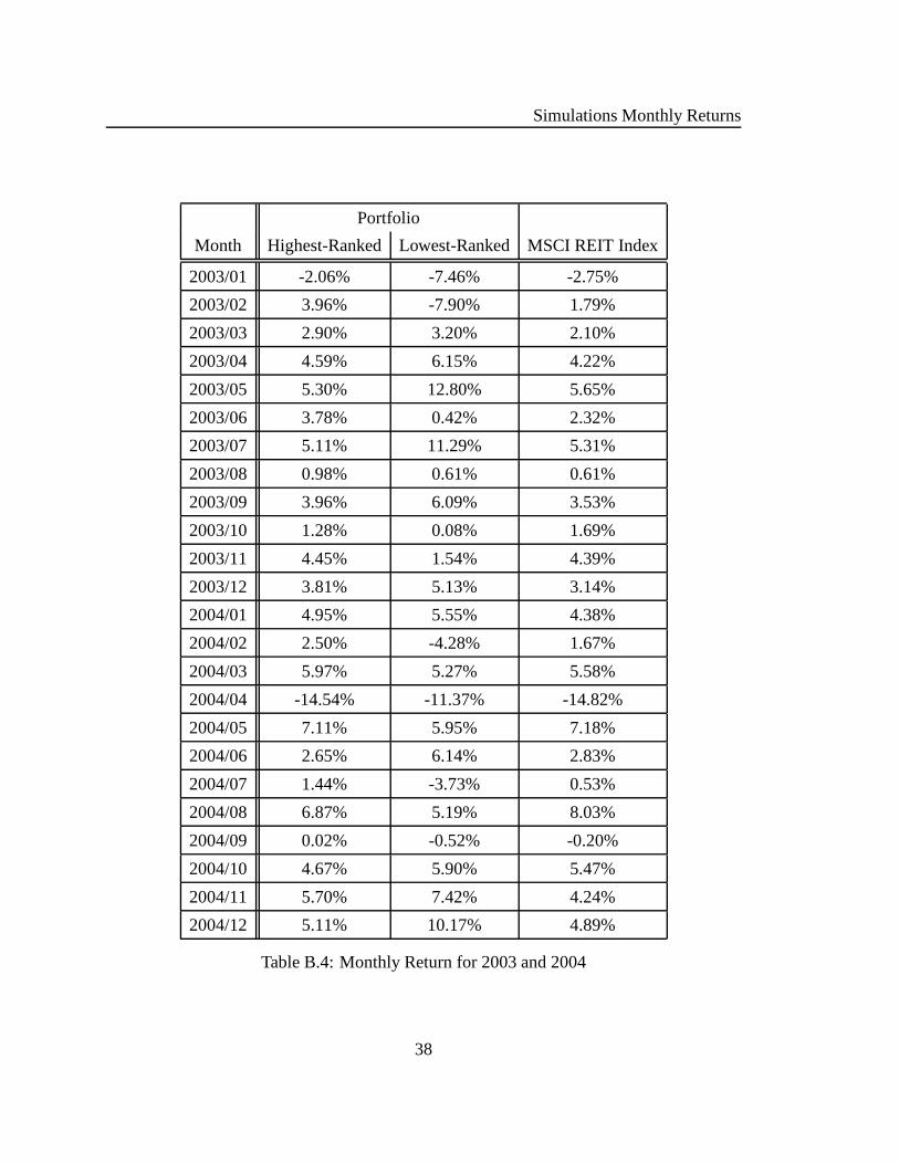
Simulations Monthly Returns

The following tables show the monthly returns of the highest- and lowest-ranked port-

folio simulations.

Portfolio

Month Highest-Ranked Lowest-Ranked MSCI REIT Index

1998/01 0.75% 0.46% -1.24%

1998/02 -1.29% -2.56% -1.61%

1998/03 3.26% 1.30% 2.37%

1998/04 -3.45% -3.15% -3.54%

1998/05 0.77% 0.48% -0.87%

1998/06 0.08% -0.40% -0.01%

1998/07 -3.65% -6.73% -7.02%

1998/08 -6.95% -12.93% -9.42%

1998/09 10.44% 6.46% 6.19%

1998/10 -1.17% -0.38% -1.89%

1998/11 -0.14% 3.87% 1.57%

1998/12 2.06% -5.23% -1.78%

Table B.1: Monthly Return for 1998

35


Portfolio


1999/01 -3.45% -1.57% -2.69%

1999/02 -4.05% -1.54% -1.64%

1999/03 1.30% 0.24% -0.55%

1999/04 12.06% 9.21% 9.67%

1999/05 2.79% 1.60% 2.12%

1999/06 -0.51% -2.95% -1.86%

1999/07 -4.88% -4.98% -3.15%

1999/08 0.73% -1.02% -0.96%

1999/09 -2.73% -5.25% -4.18%

1999/10 0.51% -1.33% -2.28%

1999/11 -3.48% -1.39% -1.48%

1999/12 3.15% 3.98% 3.11%

2000/01 0.44% -0.08% 0.62%

2000/02 -3.17% -3.08% -1.59%

2000/03 7.65% 5.67% 3.67%

2000/04 6.27% 5.25% 6.72%

2000/05 2.70% 0.46% 0.92%

2000/06 2.81% 4.46% 2.48%

2000/07 10.88% 5.33% 9.07%

2000/08 -2.57% -0.37% -4.10%

2000/09 4.23% 0.12% 3.08%

2000/10 -3.65% -5.04% -4.75%

2000/11 1.39% 3.55% 1.75%

2000/12 8.31% 3.53% 7.11%

Table B.2: Monthly Return for 1999 and 2000

36

Portfolio


2001/01 4.62% -1.12% 0.43%

2001/02 -2.36% -3.92% -1.72%

2001/03 1.50% -0.78% 0.82%

2001/04 4.58% 2.67% 2.32%

2001/05 4.78% 7.07% 2.24%

2001/06 2.82% 1.35% 6.03%

2001/07 0.33% -5.29% -2.16%

2001/08 1.78% 6.23% 3.70%

2001/09 -14.78% -2.97% -4%

2001/10 1.38% -2.08% -3.35%

2001/11 10.54% 7.34% 5.83%

2001/12 4.61% 1.66% 2.60%

2002/01 2.97% -0.66% -0.23%

2002/02 3.59% 2.16% 1.98%

2002/03 7.25% 5.50% 6.44%

2002/04 1.68% -1.16% 0.64%

2002/05 0.18% -0.45% 1.27%

2002/06 2.37% 1.51% 2.87%

2002/07 -4.95% -5.35% -5.61%

2002/08 -0.09% -2.22% 0.17%

2002/09 -1.73% -4.87% -3.63%

2002/10 -6.64% -1.89% -5.02%

2002/11 5.12% 6.02% 4.61%

2002/12 0.99% -0.67% 0.83%


37


Portfolio


2003/01 -2.06% -7.46% -2.75%

2003/02 3.96% -7.90% 1.79%

2003/03 2.90% 3.20% 2.10%

2003/04 4.59% 6.15% 4.22%

2003/05 5.30% 12.80% 5.65%

2003/06 3.78% 0.42% 2.32%

2003/07 5.11% 11.29% 5.31%

2003/08 0.98% 0.61% 0.61%

2003/09 3.96% 6.09% 3.53%

2003/10 1.28% 0.08% 1.69%

2003/11 4.45% 1.54% 4.39%

2003/12 3.81% 5.13% 3.14%

2004/01 4.95% 5.55% 4.38%

2004/02 2.50% -4.28% 1.67%

2004/03 5.97% 5.27% 5.58%

2004/04 -14.54% -11.37% -14.82%

2004/05 7.11% 5.95% 7.18%

2004/06 2.65% 6.14% 2.83%

2004/07 1.44% -3.73% 0.53%

2004/08 6.87% 5.19% 8.03%

2004/09 0.02% -0.52% -0.20%

2004/10 4.67% 5.90% 5.47%

2004/11 5.70% 7.42% 4.24%

2004/12 5.11% 10.17% 4.89%


38

Portfolio


2005/01 -8.34% -7.85% -8.61%

2005/02 2.61% -1.87% 2.92%

2005/03 -1.85% -2.76% -1.60%

2005/04 6.76% 1.40% 5.94%

2005/05 4.91% 8.53% 3.26%

2005/06 5.36% 3.85% 5.02%

2005/07 6.95% 5.47% 7.17%

2005/08 -3.03% -2.46% -3.85%

2005/09 0.93% -0.27% 0.57%

2005/10 -4.23% -1.90% -2.38%

2005/11 6.57% 6.05% 4.33%

2005/12 -0.15% 1.96% -0.10%

2006/01 5.85% 9.22% 7.68%

2006/02 3.46% 1.20% 1.88%

2006/03 6.81% 4.51% 4.97%

2006/04 -2.90% -2.49% -3.72%

2006/05 -1.82% -0.83% -2.88%

2006/06 5.01% 3.56% 5.38%


39


40

Bibliography

[And05] Anton Andriyashin. Financial applications of classification and regression

trees. Master’s thesis, Humboldt University, Berlin, March 2005.

[BEYG04] A. Borodin, R. El-Yaniv, and V. Gogan. Can we learn to beat the best stock.

Journal of Artificial Intelligence Research, 21:579–594, May 2004.

URL: <citeseer.ist.psu.edu/borodin03can.html>.

[Bre94] Leo Breiman. Bagging predictors.Machine Learning, 24(2):123–140, 1994.

URL: <ftp://ftp.stat.berkeley.edu/pub/users/breiman/bagging.ps.

[BS95] J.S. Brush and V.K. Schock. Gradient maximization: An integrated return/risk

portfolio construction procedure.Journal of Portfolio Management, 21(4),

1995.

[FSH05] Corin Frost, Amy Schioldager, and Scott Hammond. Real estate investing: the

reit way. Investment Research Journal from Barclays Global Investors, 8(7),

September 2005.

[GB96] Joumana Ghosn and Yoshua Bengio. Multi-task learning for stock selection.

In NIPS, pages 946–952, 1996.

[KV95] A. Krogh and J. Vedelsby. Neural network ensembles, cross validation and

active learning. pages 231–238. Cambridge MA: MIT Press, 1995.

41

Bibliography

[Lev95] Asriel E. Levin. Stock selection via nonlinear multi-factor models. InNIPS,

pages 966–972, 1995.

[LLM94] Asriel U. Levin, Todd K. Leen, and John E. Moody. Fastpruning using prin-

cipal components. In Jack D. Cowan, Gerald Tesauro, and Joshua Alspector,

editors,Advances in Neural Information Processing Systems, volume 6, pages

35–42. Morgan Kaufmann Publishers, Inc., 1994.

[lon99] Steven F. Freed. An Overview of Long-Short Equity Investing, William Mercer

Investment Consulting, Nov. 29, 1999.

[REI04] REITs 101: Introduction to Real Estate Investment Trusts, Citigroup Global

Markets, Sept. 29, 2004.

[whies] An Overview of the CART Methodology, Salford Systems White Paper Series.

[ZNG01] Hans-Georg Zimmermann, Ralph Neuneier, and Ralph Grothmann. Active

portfolio-management based on error correction neural networks. In NIPS,

pages 1465–1472, 2001.

42

Documents

A LINEAR MULTIFACTOR MODEL FOR REITS SELECTION USING ...ale44/MScWorkReport-LE.pdf · A LINEAR MULTIFACTOR MODEL FOR REITS SELECTION USING GRADIENT ... of the REIT on a public stock