1

A Life Cycle Assessment of Oxymethylene Ether Synthesis from

Biomass-derived Syngas as a Diesel Additive

Nafisa Mahbub1, Adetoyese Olajire Oyedun1, Amit Kumar1,1*, Dorian Oestreich2, Ulrich

Arnold2, Jörg Sauer2

1 Department of Mechanical Engineering, 10-263 Donadeo Innovation Centre for Engineering,

University of Alberta, Edmonton, Alberta T6G 1H9, Canada.

2 Institute of Catalysis Research and Technology (IKFT), Karlsruhe Institute of Technology

(KIT), Hermann-von-Helmholtz-Platz 1, 76344 Eggenstein-Leopoldshafen, Germany.

ABSTRACT

The life cycle energy consumption and greenhouse gas (GHG) emission performances of forest

biomass-derived oxymethylene ether (OME) synthesis used as a diesel additive are analyzed in

this study. OME, a new alternative liquid fuel, has great miscibility with conventional fuels like

diesel. OME can reduce combustion emissions significantly when used as a diesel additive

without any modification to the engine. A data-intensive spreadsheet-based life cycle assessment

(LCA) model was developed for OME synthesis from woodchips derived from two different

kinds of forest biomass, whole tree and forest residue. Woodchip harvesting, chip transportation,

1* Corresponding author. Tel.: +1-780-492-7797.

E-mail: Amit.Kumar@ualberta.ca (A. Kumar).

2

chemical synthesis of OME from biomass-derived syngas, OME transportation to blending, and

vehicle combustion of this transportation fuel were considered in the system boundary. The

results show that the whole tree pathway produces 27 g CO2eq/MJ of OME, whereas the forest

residue pathway produces 18 g CO2eq/MJ of OME over 20 years of plant life. The difference is

mainly due to some emissions-intensive operations involved in biomass harvesting and biomass

transportation such as skidding, road construction, etc., in the whole tree pathway. Also, vehicle

combustion was found to be the most GHG-intensive unit for both pathways. OME combustion

in a vehicle accounts for about 77% and 83% of the total life cycle GHG emissions for the whole

tree and forest residue pathways, respectively. This study also compares the diesel life cycle

emission numbers with the life cycle emissions of OME derived from forest biomass, and it was

observed that GHG emissions can be reduced by 20-21% and soot (black carbon) emissions can

be reduced by 30% using a 10% OME blended diesel as a transportation fuel compared with

conventional diesel.

Keywords: Life cycle assessment; oxymethylene ether; forest biomass; greenhouse gas

emissions; energy

Abbreviations:

ARP Acid rain precursors

CNG Compressed natural gas

CO Carbon monoxide

CO2eq Carbon dioxide equivalent

3

FU Functional unit

GHG Greenhouse gas

GOP Ground-level ozone precursors

HC Hydrocarbon

LCA Life cycle assessment

LNG Liquefied natural gas

LPG Liquefied petroleum gas

MJ Megajoule

NOx Nitrogen oxide

OME Oxymethylene ether

PM Particulate matter

VOC Volatile organic compounds

WTW Well to wheel

4

1. Introduction

Around 46 billion metric tonnes of CO2eq gases or GHGs were emitted worldwide in 2010, of

which an estimated 71% came from energy production and use alone, including fuel combustion

in vehicles (EPA, 2014). Canada emitted 702 million tonnes of CO2eq gases in 2011, and most

of these emissions came from Alberta, in particular from the petroleum industry (Environment

Canada, 2013). In 2014, Alberta generated 250 Mt of GHGs. If Alberta continues to generate

GHGs at this rate, it will produce more than 300 Mt CO2eq gases per year by 2050, which is

alarming (Mahbub and Kumar, 2014; Row and Mohareb, 2014). In 2011, Alberta generated

around 239 Mt CO2eq gases, of which almost 40% came from mining and oil gas extraction and

the subsequent use of oil and gas in production, refining, and vehicle combustion (Mahbub and

Kumar, 2014; Row and Mohareb, 2014). Vehicle exhaust in the form of CO2, soot, NOx, HC,

and CO creates environmental pollution. Carbon black, or soot, is considered to be the second

largest emission-contributing global warming material after carbon dioxide. It is responsible for

producing around 1.1 W/m2 of warming effect in the atmosphere (Bond et al., 2013). The

combustion of fossil fuels in vehicles is one of the highest potential sources of soot or black

carbon.

Oxygenated compounds are added to conventional fossil fuels as additives to reduce soot

formation (Pellegrini et al., 2012) and make combustion cleaner (Zhang et al., 2014; Zhang et al.,

2016). Oxymethylene ether (OME) is an emerging fuel that can be used as an alternative

transportation fuel or a fuel additive. The composition of oligomer molecules in OMEs can be

adjusted to match the distillation range of diesel, thus providing great miscibility with diesel. In

addition, OME can be used in old vehicles without altering the engine or using any diesel

5

particulate filter (DPF) or any other expensive maintenance device and can be produced from a

range of feedstocks including both fossil sources and biomass (Pellegrini et al., 2013).

To combat the environmental issues arising from fossil fuel combustion and fossil resource

depletion, there is a move towards the production and use of alternative fuels (Kajaste, 2014;

Nguyen et al., 2013). GHGs can be reduced considerably by replacing fossil sources with bio-

based energy sources such as whole tree biomass, forest residue, agricultural residue, etc. (Agbor

et al., 2016; Thakur et al., 2014). In Alberta, forests are harvested mainly for pulp and lumber.

Since the demand for paper is decreasing, forest biomass can be a potential source of energy that

can replace fossil sources (Government of Canada, 2016; Kabir and Kumar, 2012).

Beer and Grant (2007) discussed GHG emissions reduction from the production and use of

several biomass-derived alternative fuel blends such as diesohol (15% ethanol blended with low

sulfur diesel and an emulsifier), hydrated ethanol (azeotropic ethanol), petrohol (E10, a blend of

10% ethanol and premium unleaded petrol), and E85 (a blend of 85% ethanol, ignition improver,

and a denaturant). Pre-combustion and combustion emissions from conventional fuels (i.e.,

diesel) and several alternative fuels such as CNG, LNG, LPG, ethanol blended with 5% petrol

(E95), E10 blend (10% ethanol by volume mixed with gasoline), pure biodiesel (BD100),

biodiesel blended with 80% diesel (BD20), and 65% diesel (BD35) have been discussed in the

literature (Beer et al., 2002; Beer et al., 2003).

Among the oxygenated compounds, methanol, dimethyl ether (DME), dimethoxymethane

(DMM), and OME are the most prominent diesel additives discussed in the literature (Zhang et

al., 2014; Zhang et al., 2016). Studies have discussed different processes of fuel grade methanol

production such as direct conversion of conventional fossil fuels including NG, biomass

6

gasification, CO2 hydrogenation etc. and analyzed different process parameters on methanol

yield (Liu et al., 2016; Riaz et al., 2013). Methanol and dimethyl ether produced from renewable

sources like hydrogen from water or wind electrolysis and captured carbon dioxide (Matzen and

Demirel, 2016; Van-Dal and Bouallou, 2013) can reduce greenhouse gas emissions by 82-86%

compared to conventional fossil fuels. However, due to their chemical properties, DMM and

DME require engine modification prior to their use as diesel additives in vehicles whereas OMEs

can be used as diesel additives without any engine modification (Pellegrini et al., 2013; Zhang et

al., 2016). Burger et al. (2010) discussed the formation of OMEs from DMM and trioxane (TRI)

and also investigated the physical and chemical properties of OMEs used as diesel additives.

Zhang et al. (2014) developed a detail process model to produce OMEs from biomass and

investigated some of the key parameters affecting the process such as equivalence ratio, H2/CO

ratio, and water flow rates. The authors found that a blend of 20% OME and 80% diesel can

reduce soot emissions by 50%. Pellegrini et al. (2013) investigated the performance of neat OME

(100%) and blended OME (10% OME blended with 90% diesel) in reducing the combustion

emissions from old vehicles. Usually, a 10% blend of any oxygenated component with any

conventional transportation fuel is considered the maximum to be used in old cars (Löfvenberg,

2010; Pellegrini et al., 2013). Since the lower heating value (LHV) of OME is significantly less,

100% OME as a transportation fuel is not considered to be strong enough for highway driving

conditions (Pellegrini et al., 2013). Pellegrini et al. (2014) further investigated the polyaromatic

hydrocarbon (PAH) emissions and particle number size distribution (PNSD) in an old vehicle

fueled with 7.5% OME blended in diesel. Zhang et al. (2016) designed an optimal process model

for the production of high OMEs (such as OME3, OME4, and OME5) from woody biomass. A

7

number of studies have been conducted on process modelling of OME synthesis from methanol

(Zhang et al., 2014; Zhang et al., 2016), and there are a few studies on combustion emission

performance of OME in vehicles (Pellegrini et al., 2012; Pellegrini et al., 2013). But there is

almost no published literature on LCAs or life cycle emission performances of the whole supply

chain of OME production from biomass to be used as a diesel additive. This study focuses on the

life cycle environmental impacts of the production and combustion of OME from two different

types of woody biomass in the western Canadian province of Alberta.

OME as a fuel or fuel additive has not been discussed widely in the literature. Nor is there an

LCA of OME, which is essential to determine the environmental impacts of the technology.

Therefore, the main objective of this study is to conduct an LCA of energy and emission

performance of OMEs from whole tree and forest residue biomass in Western Canada. The

specific objectives are to:

● Develop a system boundary diagram showing the production and use of OME from

biomass;

● Develop energy consumption estimates of various unit operations for the whole chain of

OME production from biomass and the use of OMEs;

● Estimate the life cycle GHG emissions for the whole chain of OME production and use;

● Estimate the life cycle acid rain precursors (ARPs) and the ground-level ozone precursors

(GOPs) for the upstream operations;

● Conduct a sensitivity analysis to study the impact of variations in input parameters on

overall life cycle GHG emissions.

8

2. Methodology

The goal of this study is to develop a data-intensive spreadsheet-based LCA model for OME

synthesis from woodchips derived from two different types of forest biomass, whole tree and

forest residue, and calculate the GHG emissions and net-energy-ratio (NER). The net energy

ratio is the ratio of total energy output from the system to the total non-renewable energy input to

the system (Shahrukh et al., 2015; Spitzley and Keoleian, 2004). Information from the literature

and Alberta-specific assumptions (such as biomass yield, biomass harvest area, moisture content,

and tortuosity factor for biomass transportation distance) and current practices were used to

evaluate energy consumption and GHG emissions.

In this study, a life cycle assessment of OME synthesis from two different types of forest

biomass was carried out. The system boundary was made up of the following six unit operations

for both pathways: biomass production, biomass transportation, chemical conversion, fuel

mixing, fuel dispensing, and vehicle combustion. The unit operations were further divided into

subunit operations for both biomass feedstock pathways (see Fig. 1). Due to the lack of data and

relatively less significance on overall life cycle emissions, the downstream operations such as

fuel dispensing, blending, storage, etc., were not included.

The results are given using a functional unit (FU) of 1 MJ of heat produced from OME so that

the LCA results can be compared with the results of other LCA studies.

Three gases – carbon dioxide (CO2), methane (CH4), and nitrous oxide (N2O) – are considered to

cause global warming. Their relative impact on global warming is assumed to be 1, 34, and 298

times, respectively (Myhre et al., 2013). A 100-year time horizon is assumed for this impact. The

9

acid rain precursors (ARPs) are sulfur dioxide (SO2) and nitrogen oxide (NOx), which are

considered mainly responsible for acidification. The weighting factor for ARPs (SO2eq) is

considered to be 1 for SO2 and 0.7 for NOx. The ground-level ozone precursor (GOP) was also

calculated in this study. GOPs include NOx and volatile organic compounds (VOC). Both of

these compounds have a weighting factor of 1 as GOPs. In the presence of sunlight, NOx and

VOC react with each other chemically and create ground-level ozone (Kabir and Kumar, 2011;

Perera and Sanford, 2011).

3. Life Cycle Inventory

Both pathways studied here involve biomass production, biomass transportation, OME synthesis

from biomass-derived syngas, transportation of OME, blending, and fuel combustion in a

vehicle. As mentioned above, downstream operations like fuel mixing, storage, distribution,

distillation, etc., are not considered in this study. This study considers a plant (gasifier) capacity

of 277 t/d for OME synthesis. The GHG emissions are calculated over 20 years of plant life and

the results are given in g CO2eq/MJ of OME. The results are also compared to conventional

diesel emission numbers.

3.1 Biomass Production

For whole tree harvesting in Alberta, trees are cut in the stand, skidded to the roadside and

delimbed, and, eventually, the trunk is used by pulp and paper industries (Pulkki, 1997;

Shahrukh et al., 2016b). The biomass harvesting unit operation includes the subunit operations

felling, skidding, and chipping (Fig. 1). The energy and emission impacts from manufacturing,

operations, and disposal of the equipment used (feller, skidder, chipper) are also considered.

Silviculture operations, which include fertilizing and pesticide spraying, are not considered in the

10

base model because in Alberta it is assumed that first-generation trees are harvested. However, a

case described later in the sensitivity analysis (section 4.4) was developed that includes the

energy and emission impacts from silviculture operations.

Fig. 1

In Alberta, the rotation of whole tree growth is assumed to be 100 years; this time frame was

determined based on weather and soil conditions. Whole forest yield includes both hardwood and

softwood. It is assumed in this study that 84 dry tonnes of forest biomass are harvested per

hectare and that 20% of whole tree biomass is forest residues (Alberta Energy, 1985; Kumar et

al., 2003). Thus the yield of forest harvest residue is assumed 0.247 dry tonnes per hectare over a

100-year rotation. The current trend in Alberta is to burn the residues to prevent forest fires

(Shahrukh et al., 2016a). The removal of forest residues removes nutrients required for forest

growth that would otherwise be returned to the soil. It is assumed in this study that ash (from the

bio-plant) would be returned to the forest floor after the biomass is used for fuel production and

thus forest soil nutrients are balanced (Thakur et al., 2014; Wihersaari, 2005). As the nutrient

system can be balanced (through ash replacement) and the residues are otherwise considered

waste (by their burning), forest harvest residues can be considered a good source for bioenergy

production . Table 1 shows the data and assumptions for biomass harvesting for both the whole

tree and forest residue pathways.

Table 1

11

The forest residue pathway includes forwarding and chipping (See Fig. 1). The energy and

emission impacts from production, operations, and disposal of the equipment used (forwarder

and chipper) were also considered in this study.

Steel is used in the construction of all types of equipment and machines (e.g., fellers, skidders,

forwarders, chippers, and transportation vehicles) considered in this study over the entire life

cycle for both pathways.

Diesel is the fuel used to operate the machinery and equipment. Natural gas is used during the

conversion of OME from biomass for syngas cleaning. The life cycle energy and combustion

emission factors for different material and fuels considered in the system boundary for both

pathways were taken from literature (Kabir and Kumar, 2012; Pellegrini et al., 2013; Stripple,

2001). The energy and emission factors are given in Table 2. The specifications of equipment

used in biomass processing and harvesting for both pathways are given in Table 3. Energy and

emission impacts from construction, operation, and disposal of equipment and machinery were

considered in the system boundary.

Table 2

Table 3

3.2 Biomass Transportation

A circular biomass harvest area is assumed for both pathways. Biomass collection distance

depends on two other aspects, tortuosity and geometric factors. The tortuosity factor is the ratio

of the distance travelled for biomass collection divided by the visible biomass collection

distance, and the geometric factor is used to measure the biomass distribution over the harvest

12

area. A circular harvest area growing only a biomass feedstock has a geometric factor of one, and

the tortuosity factor was assumed in this study (for practical transportation assumptions) to be

1.27 (Overend, 1982). We assumed that the preprocessing plant was situated at the center of the

harvest area. This methodology has been used in earlier studies (Shahrukh et al., 2016b). With

these assumptions, the biomass collection distances used for the whole tree and forest residue

pathways were 4.56 km and 21.75 km, respectively (Thakur et al., 2014).

Biomass is transported in heavy capacity trailer trucks. Fourteen tonnes of steel are used to

manufacture a trailer truck. A trailer truck can carry 23 wet tonnes of biomass in a single trip and

travel up to 2.55 km/L of fuel when empty and 2.12 km/L with a load (Kabir and Kumar, 2012;

Mann and Spath, 1997). The energy and emission impacts of truck construction and operation

are included in this study.

For the whole tree pathway, road construction was considered as a subunit operation. Forest

roads are classified as primary, secondary, and tertiary. Whole trees are usually slid to a primary

roadside and chipped, and the chips are transported by truck on primary roads. Other harvesting

machinery like fellers, skidders and chippers operate on secondary and tertiary roads on slow

speed.

For an OME plant with a capacity of 277 dry tonnes of biomass per day, around 36.48 km of

primary road, 42.98 km of secondary road, and 28.65 km of tertiary road construction were

assumed for the whole tree pathway in this study. The road construction estimates are based on a

discussion with Fulton Smyl (Business Analyst, Alberta Innovates-Technology Futures on June

28, 2016) on Alberta’s forest management plans, roads classification, and design specifications.

The energy and emission factors for primary road construction – 1731 GJ/km, 403,845 kg

13

CO2eq/km, 1015 kg SO2eq/km, and 1155 kg (NOx + VOC)/km – are taken from previous studies

(Kabir and Kumar, 2011, 2012; Stripple, 2001). Crawler tractors (140 horsepower /105 kilowatt)

are assumed to be used for secondary and tertiary road construction (Winkler, 1998). Primary

roads are generally built as permanent roads, whereas secondary roads are built to be semi-

permanent and tertiary roads are temporary trails mostly used for harvesting (Ontario Ministry of

Natural Resources, 1994). Hence, the tractor operating hours are considered to be 70 h/km for

secondary road and 100 h/km for tertiary road construction in this study (Table 3) (Winkler,

1998).

For the forest residue pathway, no road construction is required. The chips are assumed to be

transported using the existing road network used by regular logging companies (Kabir and

Kumar, 2011, 2012; Shahrukh et al., 2016b).

We calculated truck fuel consumption using a formula from Sultana and Kumar (2011), given in

Equation 1. We assumed that a truck carries less than its payload, or volumetric capacity. Truck

fuel consumption is calculated as follows:

(1)

where Fa = actual fuel consumed by a truck while carrying a load La (L/km), Fe = fuel consumed

by an empty truck (L/km), Ff = fuel consumed by a fully loaded truck (L/km), La = actual load

transported by a truck (t), and Lp= volumetric capacity of a truck (t). The inventory data for

biomass transportation are given in Table 1.

14

3.3 OME Plant Construction

An OME plant is assumed to have 20 years of plant life. Due to similarities in the chemical

conversion of OME with other fuels like biohydrogen production (such as biomass gasification,

syngas cleaning, H2/CO adjusting, etc.), the scale factor needed to determine the amount of

material to construct an OME plant is taken from existing literature on other plants (Moore,

1959; Spath and Mann, 2000). The amount of construction material was determined through

Equation 2 obtained from Sarkar and Kumar (2010a, b):

(2)

Here, Si = the size of the OME plant, So = the size of reference plant, Ci = the amount of material

required for an OME plant, So = the amount of material in the reference plant, and n= the scale

factor. A scale factor of 0.76 was assumed in this study. The scale factor was taken from Kabir

and Kumar (2011) due to similarities in biohydrogen production operations and OME synthesis.

As an example, for a Battelle Columbus Laboratory (BCL) plant with a capacity of 250,200 kg

H2/ day, Kabir and Kumar (2011) estimated the amount of steel, concrete, and aluminium to be

5350, 16,535, and 44 t, respectively. We used these values as reference plant material amounts in

Equation 2 and a scale factor of 0.76 and estimated the amount of material for an OME plant

(capacity 24,746 kg OME/day) to be 922 t steel, 2850 t concrete, and 7.58 t of aluminium. The

energy and emission impacts of plant decommissioning and disposal of construction material are

also included in the plant construction unit operation. The energy and emission impacts from

plant decommissioning are assumed to be 3% of plant construction impacts (Elsayed and

Mortimer, 2001; Kabir and Kumar, 2011). The construction materials are assumed to be disposed

15

of in landfills 50 km from the plant (Kabir and Kumar, 2011, 2012; Spath et al., 2005). Heavy

capacity trucks used in biomass transportation are used for construction material disposal. All

aluminium and concrete material are assumed to be landfilled, but 75% of the steel is recycled

and 25% of it is landfilled (Spath et al., 2005; Spath and Mann, 2000). The energy and emission

factors for steel and aluminium landfilling are 0.01 tCO2eq/t material and, for concrete, 0.044

tCO2eq/t material (Spath et al., 2005; Spath and Mann, 2000).

3.4 Chemical Conversion

Five subunit operations are included in the chemical conversion process: gasification, syngas

cleaning and H2/CO adjustment, methanol synthesis, OME synthesis, and ash disposal. Both

feedstocks undergo the same process. Biomass conversion is considered to be carbon neutral as

all carbon released during the combustion of the woodchips is compensated by the amount of

carbon up taken during forest growth (Hartmann and Kaltschmitt, 1999; Liu et al., 2013; Zhang

et al., 2009). The input-output mass flow rates for chemical conversion unit operations are given

in Table 4. The output includes OMEs 1 to 8 and some untreated gases such as N2, O2, water, etc.

6.80 MW of external heat energy, supplied by natural gas, are used in syngas cleaning and

H2/CO adjustment unit operations (Zhang et al., 2016). But this external energy is a small

fraction (around 6.57%) of the energy consumed during the whole chemical conversion process.

The remaining heat energy is supplied by the combustion of 13 – 17% of the input biomass

depending on the biomass feedstocks as stated by Zhang et al. (2016).

Table 4

The ash contents in whole tree and forest residue biomass are assumed to be 1% and 3%,

respectively (Van den Broek et al., 1995; Kumar et al., 2003). Over 20 years, 16,986 t and

16

50,957 t of ash are produced through the whole tree and forest residue pathways, respectively.

The ash is assumed to be disposed of 50 km away from the plant in the forest area and is usually

considered to replace the nutrients removed with the trees and residues (Kumar et al., 2003;

Spath et al., 2005). The same heavy capacity trailer trucks used in biomass transportation are

used to spread ash. The ash spreading rate is assumed to be 1 t/ha, and a 40' fertilizer spreader

with a capacity of 4.41 ha/h is used (Kabir and Kumar, 2011; Spath et al., 2005). The life cycle

energy and emission impacts of trucks and spreaders used for ash transportation and ash

spreading are included in this study.

3.5 OME Transportation

In this study, we assumed a distance of 300 kilometers to transport OME from the chemical

conversion plant to the blending plant. We also assumed that the high capacity trailer trucks used

for biomass transportation and ash disposal would be used for OME transportation. The energy

and emissions impacts of construction and operation of trucks are considered in this study.

3.6 Vehicle Combustion

Combustion emissions and fuel consumption numbers are taken from a study by Pellegrini et al.

(2013). They tested an in-use diesel engine car with three different types of fuel, conventional

diesel, 100% OME, and a 10% OME diesel blend. The particulate matter (PM) emissions were

also calculated, and the PM composition determined the amount of soot emissions. Pellegrini et

al. (2013) found that 77% of diesel PM emissions are black carbon/soot whereas in OME, only

33% of PM emissions are black carbon/soot and 50% of the PM emissions come from the

volatile organic fractions in lube oil. These figures are used in our model to calculate the soot

emissions from vehicle combustion. The soot emissions for 100% OME and a 10% OME blend

17

with diesel as calculated in this model are 0.0011 g/MJ of OME and 0.0071 g/MJ of OME,

respectively. When a strong oxidation catalyst and a good synthetic lubricant in vehicles are

used, PM emissions can be further reduced. According to the experimental results by Pellegrini

et al., using 100% OME as a transportation fuel can reduce soot emissions significantly, although

hydrocarbon (HC), carbon monoxide (CO), nitrogen oxides (NOx), and carbon dioxide (CO2)

emissions and fuel consumption increase (Pellegrini et al., 2013). The CO2eq emissions from the

combustion of 100% OME as a transportation fuel are considered to be zero in our model since

we assume that the combustion emissions of biomass-derived fuels are compensated by the

amount of CO2 taken up by the tree during its growth. The combustion emissions from a 10%

OME blend with diesel are around 0.060 CO2eq/MJ of OME and come predominantly from the

diesel fraction.

4. Results and Discussion

In this section, the results of the life cycle energy and emission impact assessments for both

whole tree and forest residue pathways are presented, compared, and discussed. The sensitivity

analyses for the different scenarios are also discussed.

4.1 Life Cycle Energy and Emission Impacts for the Whole Tree Pathway

Table 5 shows the energy consumptions and GHG emissions results for the upstream operations

from whole tree biomass.

Table 5

Of the upstream unit operations (biomass production, biomass transportation, and chemical

conversion), chemical conversion consumes the most energy, almost 85% of the energy

18

consumed in the pathway. The primary energy input for chemical conversion is the heat from the

wood chips, which is around 26.37 MW (equivalent to 8.215 MJ/kg). The output from one

subunit operation is used as input for the next. About 6.80 MW of fossil heat energy (from

natural gas) are used in the syngas cleaning and H2/CO adjusting subunit operation; this is the

only fossil energy considered in chemical conversion operation. Biomass harvesting is the

second most energy-intensive unit operation, and biomass transportation consumes the least

energy over the entire life cycle of whole tree pathway.

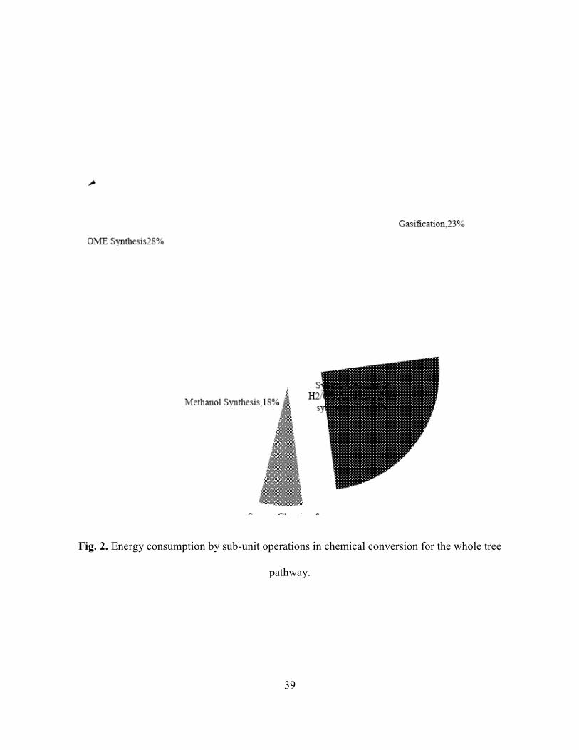
For chemical conversion, OME synthesis in the whole tree pathway consumes the most energy,

around 28% of the energy used in the conversion (Fig. 2). The energy required in gasification

(around 23% of the energy consumed in chemical conversion) comes primarily from the biomass

(wood chips). The fossil energy used in this pathway is around 6.57%, which is supplied by

natural gas.

Fig. 2

Equipment construction energy is negligible compared to equipment operation energy for all the

biomass harvesting equipment considered in this study.

Around 40% of the energy used in the whole tree pathway is consumed in skidding operations.

For this study, 19 skidders with a productivity of 7.5 dry tonnes whole trees per hour are required

for a plant capacity of 277 t/d over 20 years (Table 3). A skidder’s hourly productivity is

comparatively much lower than that of a feller (8.75 dry tonnes whole trees per hour) or a

chipper (30 dry tonnes whole trees per hour for a high-efficient chipper). But a skidder’s life

cycle fuel consumption is higher than that of a feller (Table 3), making it the highest energy-

19

consuming unit in biomass production. Only six high-efficient chippers are required over 20

years, hence chipping is the least energy consuming unit (around 22%) throughout the life cycle

(Table 3).

Vehicle combustion is the most GHG emissions-intensive unit, contributing around 77% of life

cycle GHG emissions in the whole tree pathway. However, this unit operation is considered to be

carbon neutral, thereby nullifying the effect of GHG emissions. Biomass production produces the

second highest GHG emissions and contributes 12% of emissions over the life cycle.

In this study, it was assumed that 36.5 km of primary roads were constructed in order to haul

whole tree biomass from the forest. This is the third most emissions-intensive unit operation

(5.35% of total life cycle GHG emissions) when using whole tree biomass as an energy source.

The impact of this subunit operation on the entire life cycle emissions is discussed in the

sensitivity analysis.

Biomass production contributes around 12% of the GHG emissions over the entire life cycle for

the whole tree pathway. For biomass production, the skidder operation is the most emissions-

intensive unit (Fig. 3). Because of its relatively lower productivity and comparatively higher fuel

consumption compared to the other unit operations, skidder operations contribute the most GHG

emissions over the whole tree pathway life cycle, around 40%. The fellers contribute 36% of the

life cycle GHG emissions followed by chipper operation emissions, which are around 22%.

Equipment construction emissions are negligible compared to equipment operation emissions.

Fig. 3

20

Over the entire life cycle of the whole tree pathway, the chemical conversion unit process

contributes very few GHG emissions (only 4.82%); this result is mainly based on the

assumptions that the amount of CO2 released during the gasification of the forest biomass is

equal to the amount of CO2 taken up by the tree during its growth and the amount of external

fossil energy used during chemical conversion is negligible (only 6.57% of life cycle energy

consumption). The GHG emissions from ash disposal, including ash transportation and ash

spreading, are included in this unit operation. OME transportation emits the fewest GHGs over

the entire life cycle, only 0.43 % of life cycle GHG emissions.

The biomass production unit operation contributes the highest ARP emissions, around 62% of

the life cycle ARP emissions. The biomass transportation, chemical conversion, and OME

transportation unit processes contribute around 17%, 18%, and 2% of the life cycle ARP

emissions, respectively. Due to the lack of data, ARP and GOP emissions were not calculated for

the downstream unit operation, combustion in vehicles, for either pathway.

GOP emissions for biomass production, biomass transportation, and chemical conversion are

around 0.09 g (NOx +VOC)/MJ, 0.018 g (NOx +VOC)/MJ, and 0.02 g (NOx +VOC)/MJ

respectively. GOP emissions from the OME transportation unit operation are negligible, around

2% of the life cycle GOP emissions.

4.2 Life Cycle Energy and Emission Impacts for the Forest Residue Pathway

Table 6 shows the preliminary energy consumption and GHG emissions results for the upstream

operations from forest residue biomass.

Table 6

21

Whole tree and forest residue biomass feedstocks use the same chemical conversion process.

Thus, as for the whole tree pathway, chemical conversion is the highest energy-consuming

upstream unit operation in the forest residue pathway, around 89% of the life cycle energy,

followed by biomass production, biomass transportation, and OME transportation, which

consume around 9%, 1.3%, and 0.47% of the energy, respectively. Among the four unit

operations, vehicle combustion emits the most GHGs, around 83% of the life cycle GHG

emissions.

Biomass production produces 9.5% of the GHG emissions over the entire life cycle, followed by

chemical conversion, biomass transportation, and OME transportation at around 5%, 1.35%, and

0.47% of life cycle GHG emissions, respectively. The transportation emissions are low mainly

because no road construction is considered for the forest residue pathway (existing roads built for

logging operations are used). Similar to the whole tree pathway, chemical conversion emissions

are almost carbon neutral and hence contribute only 5% of the life cycle GHG emissions.

Equipment construction emissions are also negligible compared to equipment operation

emissions, as for the whole tree pathway. Around 50% of biomass production emissions are from

forwarder operation emissions due to the forwarder’s low productivity. For an OME plant with a

capacity of 277 t/d, around 17 forwarders are required throughout the 20 years of plant life. Six

highly productive (more than twice the productivity of a forwarder) chippers are used over 20

years of plant life, producing 47% of the biomass production emissions, almost the same as that

from forwarders.

Similar to the whole tree pathway, ARP emissions are highest for the biomass production unit

operation (around 61% of the life cycle ARP emissions), followed by the chemical conversion,

22

biomass transportation, and OME transportation operations, which contribute around 26% , 9%,

and 3% of the total life cycle ARP emissions, respectively.

In the forest residue pathway, biomass production GOP emissions are 66% of the total life cycle

GOP emissions, and chemical conversion, biomass transportation, and OME transportation

contribute around 22%, 9%, and 3% of the life cycle GOP emissions, respectively. OME

transportation contributes the lowest GOP emissions, around 0.003 g (NOx +VOC)/MJ of OME.

4.3 Comparison of Life Cycle Energy and Emission Impacts between the Two Pathways

Figure 4 shows the life cycle energy consumption of four unit operations – biomass production,

biomass transportation, chemical conversion, and vehicle combustion – in the whole tree and

forest residue pathways.

Fig. 4

Both pathways use the same chemical conversion process, and chemical conversion is the most

energy-intensive upstream operation for both (around 80-85%). Since road construction is

considered in the whole tree and not the forest residue pathway, biomass transportation energy

consumption in the whole tree pathway is twice as high as in the forest residue pathway (even

though the transportation distance for biomass collection in the forest residue pathway [21.75

km] is almost 5 times higher than in the whole tree pathway [4.56 km]). However, biomass

production energy in the whole tree pathway is higher than that of the forest residue pathway.

This is due to the effects of the subunit operations involved in biomass production. In the whole

tree pathway, biomass production has three subunit operations (skidding, felling, and chipping),

and skidding consumes the most energy (almost 40% of the energy consumed in biomass

23

production). In the forest residue pathway, the biomass production unit includes only forwarding

and chipping, neither of which consumes large amounts of energy.

For both pathways, vehicle combustion produces the highest GHG emissions, around 89.55 g

CO2eq/MJ of OME. In the whole tree pathway, vehicle combustion contributes around 77% of

the life cycle GHG emissions and in the forest residue pathway, vehicle combustion is

responsible for 83% of the life cycle GHG emissions (see Fig. 5). Since OME is produced from

biomass, combustion emissions are considered to be carbon neutral. Hence 83% of life cycle

GHG emissions in the forest residue pathway and 77% in the whole tree pathway are considered

carbon neutral, and thus the forest residue pathway produces fewer GHGs than the whole tree

pathway. In both pathways, the second highest GHG emissions come from biomass production

(around 12% of the life cycle emissions from the whole tree and 9.5% from the forest residue

pathway). Biomass transportation emissions in the whole tree pathway are almost four times

higher than those of the forest residue pathway (Fig. 5). This is mainly due to the emissions-

intensive unit operation road construction. About 36.5 km of primary road construction is

considered in the whole tree pathway.

Fig. 5

Around 12% of life cycle emissions come from biomass production in the whole tree pathway

and 9.5% the forest residue pathway. GHG emissions from whole tree and forest residue biomass

production are 14.25 g CO2eq/MJ and 10.15 g CO2eq/MJ, respectively. GHG emissions from

whole tree biomass production are higher because of the differences in biomass production

energy consumption, as explained earlier.

24

GHG emissions from chemical conversion are around 5.67 g CO2eq/MJ in the forest residue

pathway and 5.61 g CO2eq/MJ in the whole tree pathway. The difference is due to the higher ash

content in forest residues. Because of the higher ash content, this pathway produces more ash

than the whole tree pathway, thereby contributing slightly higher GHG emissions.

With respect to ARP emissions, biomass production is the highest contributor in both pathways.

Whole tree biomass production produces around 0.06 g SO2eq/ MJ and forest residue biomass

production contributes 0.04 g SO2eq/MJ (see Tables 5 and 6).

The highest GOP emissions come from whole tree biomass production and are around 0.09 g

(NOx +VOC)/MJ (see Table 5). The forest residue pathway also generates the highest GOP

emissions from biomass production unit operations; these are around 0.06 g (NOx +VOC)/MJ

(see Table 6).

4.4 Comparison with Diesel Life Cycle Energy and Emission Impacts

We compared life cycle GHG emission numbers of OME derived from forest biomass to those of

the conventional fossil fuel diesel. Several LCA studies have been published on diesel life cycle

emissions (Garg et al., 2013; Gerdes and Skone, 2009; Rahman et al., 2015). The diesel GHG

emission numbers include emissions from crude recovery, crude transportation to the refinery,

crude refining, transportation and distribution of finished fuels to the dispensing station, and

combustion of fuels in vehicles. The upstream GHG emission numbers, from crude recovery to

dispensing fuel, are taken from Rahman et al. (2015), and the combustion emission numbers for

diesel are taken from Pellegrini et al. (2013).

25

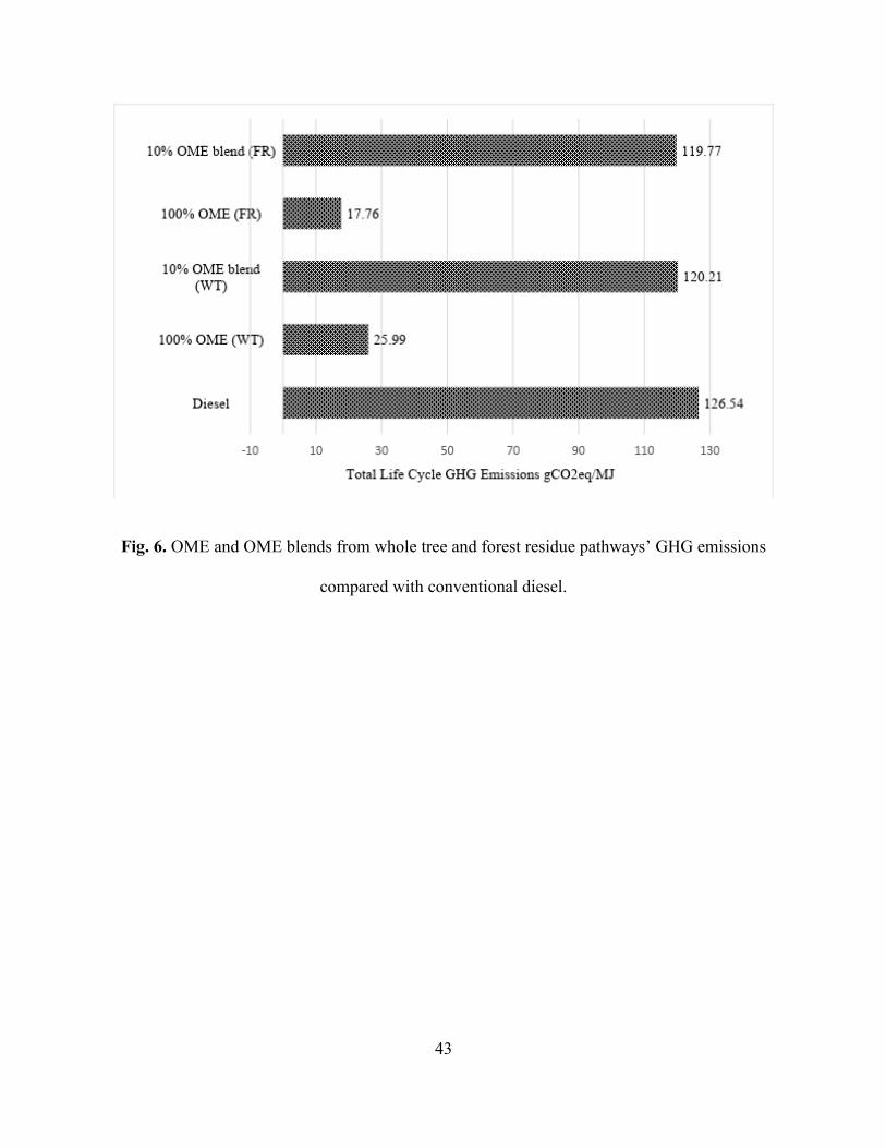
The well-to-wheel (WTW) diesel life cycle GHG emissions calculated by Rahman et al.

(2015)were 126.54 g CO2eq/MJ, whereas in this study the life cycle GHG emissions from 100%

OME as a transportation fuel were found to be 27g CO2eq/MJ when OME is produced from

whole trees and 18g CO2eq/MJ when OME is produced from forest residues (Fig. 6). In the

OME pathways, GHG emissions from vehicle combustion are assumed to be carbon neutral and

the chemical conversion process is assumed to be almost carbon neutral since only 6.57% of life

cycle energy consumption comes from a fossil source. Hence, total life cycle emissions from

OME pathways are significantly lower than those of diesel. Total life cycle GHG emissions and

percentage reductions in GHGs compared to conventional diesel for 100% OME and a 10%

OME blend with diesel to be used as transportation fuels are given in Table 7. The upstream

emissions from the forest residue pathway (18g CO2eq/MJ) are significantly lower than those of

the whole tree pathway (27 g CO2eq/MJ). Hence, 100% OME as a transportation fuel from the

forest residue pathway contributes 86% fewer GHG emissions than diesel, whereas 100% OME

from the whole tree pathway contributes 79% fewer GHG emissions than diesel. Similarly, when

OME is used as a diesel additive, for the 10% OME blended with 90% diesel, the life cycle GHG

emissions are reduced by 5% and 5.35% compared to that of diesel, when OME is produced

from the whole tree and forest residue pathways, respectively. Upstream emissions are allocated

to the OME blends depending on their mass in the finished fuel.

Fig. 6

The soot emissions for 100% OME and a 10% OME blend with diesel as calculated in our model

are 0.0011 g/MJ of OME and 0.0071 g/MJ of OME, whereas the soot emissions from diesel are

0.01 g/MJ of diesel (Pellegrini et al., 2013). We compared the soot emissions from a 10% OME

26

blend and 100% OME to the soot emissions from diesel and found that soot emissions decrease

by 30% and 89% compared to diesel for a 10% OME blend with diesel and 100% OME,

respectively. The soot emissions for all three fuels are shown in Table 7.

4.5 Sensitivity Analysis

A number of scenarios were developed for both pathways by varying parameters and

assumptions of upstream operations, and the impacts of these variations on life cycle energy and

emissions are given in Table 8. The scenarios were developed independently of each other and

compared with the base scenario. The downstream operation (vehicle combustion) is not

included in this analysis. Four scenarios were developed for the forest residue pathway and six

for the whole tree pathway.

In scenario 1, the change in capacity factors for both pathways was analyzed. The pathways were

analyzed for two sets of capacity factors: set one at 0.7 for year 1, 0.8 for year 2, 0.95 from year

3 onwards and set two at 0.65 for year 1, 0.7 for year 2, 0.75 from year 3 onwards. Life cycle

energy and emissions increased with the increased capacity factors for both pathways, and, in the

forest residue pathway, both increase significantly. As an example, GHG emissions increased

around 9% over the base scenario in the forest residue pathway with the increased capacity

factors (see Table 8). Scenario 2 demonstrates the effects of a 10% increase and decrease in

biomass yield. When the yield increases, life cycle energy consumption and emissions drop for

both pathways, and when yield decreases, energy consumption and emissions increase. But the

changes are insignificant and are within ±1%. Scenario 3 looks at the effects of a 10% increase

and a 10% decrease in biomass moisture content for both pathways. The impact is small and is

within ±1%. In scenario 4, we analyzed life cycle emission and energy consumption impacts by

27

changing the capacity by ±10%. Overall energy consumption and emissions increase with

increased capacity, but the energy consumption per unit output (per tonne of OME produced)

decreases as the capacity increases. For the whole tree pathway, a fifth scenario was developed

considering silviculture, which involves the application of fertilizer and pesticides and considers

machinery fuel consumption. Energy consumption and emissions increases were negligible.

Scenario 6 demonstrates the impact of excluding road construction operations in the whole tree

pathway. Road construction is assumed to be an emissions-intensive operation in the whole tree

pathway. We found that the energy consumption and life cycle emissions dropped significantly

compared to the base scenario. The GHG emissions also dropped considerably, by around 33%

compared to base scenario, and the other two emissions, ARP and GOP, dropped to 32% and

24% of the base scenario, respectively. Life cycle energy consumption was reduced by 4% from

the base scenario (Table 8).

5. Conclusion

This study determined the overall life cycle emissions of OME derived from two different types

of forest biomass, whole tree and forest residue, and used as a diesel additive. The life cycle

GHG emissions of OME from the whole tree and forest residue pathways are 27 g CO2eq/MJ

and 18 g CO2eq/MJ, respectively. The results show that a 10% OME blend with diesel reduces

GHG and soot emissions by 20-21% and 30%, respectively, compared to 100% diesel. Based on

these results, it is obvious that OME, when used as a diesel additive, can decrease GHG

emissions significantly compared to conventional diesel. This model can be used to design an

optimal process for maximizing OME production and minimizing energy consumption and GHG

emissions. The model can also be used to determine the optimum fuel mix (OME-diesel blend)

28

contributing the lowest GHG emissions. We recommend for further studies that the model be

extended to include other feedstocks such as agricultural residues, wood waste, or fossil fuels to

produce OME and other modes of biomass transportation such as bales, pellets, etc. The results

of this study will be of great interest to policy makers, petroleum-based fuel producers, and

biofuel companies on the environmental impacts of blending OME with diesel fuels.

Acknowledgements

The authors would like to acknowledge the partners in the Helmholtz-Alberta Initiative, the

Helmholtz Association, and the University of Alberta, whose financial support has made this

research possible. Also the authors would like to acknowledge the researchers of KIT (Karlsruhe

Institute of Technology) for their help in providing experimental data. Astrid Blodgett is

acknowledged for editorial assistance.

References

Agbor, E., Oyedun, A.O., Zhang, X., Kumar, A., 2016. Integrated techno-economic and

environmental assessments of sixty scenarios for co-firing biomass with coal and natural

gas. Appl Energ 169, 433-449.

Alberta Energy, 1985. Alberta Phase 3 Forest Inventory - An Overview. Alberta Energy and

Natural Resources. Available from: https://archive.org/details/albertaphase3for00albe

(Accessed Date: October 20, 2016).

Beer, T., Grant, T., 2007. Life-cycle analysis of emissions from fuel ethanol and blends in

Australian heavy and light vehicles. J. Clean. Prod. 15, 833-837.

29

Beer, T., Grant, T., Williams, D., Watson, H., 2002. Fuel-cycle greenhouse gas emissions from

alternative fuels in Australian heavy vehicles. Atmos. Environ. 36, 753-763.

Beer, T., Olaru, D., Van der Schoot, M., Grant, T., Keating, B., Hatfield Dodds, S., Smith, C.,

Azzi, M., Potterton, P., Mitchell, D., 2003. Appropriateness of a 350 Million Litre Biofuels

Target: Report to the Australian Government Department of Industry, Tourism and

Resources. CSIRO, ABARE, BTRE, Canberra.

Bond, T.C., Doherty, S.J., Fahey, D., Forster, P., Berntsen, T., DeAngelo, B., Flanner, M., Ghan,

S., Kärcher, B., Koch, D., 2013. Bounding the role of black carbon in the climate system: A

scientific assessment. J. G. R. Atmospheres 118, 5380-5552.

Burger, J., Siegert, M., Ströfer, E., Hasse, H., 2010. Poly (oxymethylene) dimethyl ethers as

components of tailored diesel fuel: Properties, synthesis and purification concepts. Fuel 89,

3315-3319.

Desrochers, L., Puttock, D., Ryans, M., 1993. The economics of chipping logging residues at

roadside: a study of three systems. Biomass Bioenerg. 5(6), 401-411.

Elsayed, M., Mortimer, N., 2001. Carbon and energy modelling of biomass systems: conversion

plant and data updates. Harwell Laboratory, Energy Technology Support Unit. Report No:

ESTU B/U1/00644/REP and DTI/Pub URN 01/1342.

Environment Canada, 2013. In: National inventory report: greenhouse gas sources and sinks in

Canada Part 1. Canada’s 2013 UNFCCC Submission; p. 171–97.

30

EPA, 2014. Climate Change Indicators in the United States: Global Greenhouse Gas Emissions.

United States Environmental Protection Agency. Available from:

https://www3.epa.gov/climatechange/pdfs/print_global-ghg-emissions-2014.pdf (Accessed

Date: June 15, 2016).

Garg, A., Vishwanathan, S., Avashia, V., 2013. Life cycle greenhouse gas emission assessment

of major petroleum oil products for transport and household sectors in India. Energy Policy

58, 38-48.

Gerdes, K., Skone, T., 2009. An evaluation of the extraction, transport and refining of imported

crude oils and the impact on life cycle greenhouse gas emissions. National Energy

Technology Laboratory. Report No: DOE/NETL-2009/1362. Available from:

http://www.netl.doe.gov/energy

analyses/pubs/PetrRefGHGEmiss_ImportSourceSpecific1.pdf (Accessed Date: April 20,

2016).

Government of Canada, 2016. Forestry: Region of Western Canada and the Territories: 2014-

2016. Available from: http://www.edsc.gc.ca/img/edsc-

esdc/jobbank/SectoralProfiles/WT/2A71-RPT-SectProf_WT_Forestry_EN--GEN-

20150827-VF-MR.pdf (Accessed Date: October 21, 2016).

Han, H. S., Renzie, C., 2001. Snip & skid: partial cut logging to control mountain pine beetle

infestations in British Columbia. Prince George, BC: University of Northern British

Columbia. Available from:

https://www.researchgate.net/profile/Han_Sup_Han/publication/228732211_Snip_skid_par

31

tial_cut_logging_to_control_mountain_pine_beetle_infestations_in_British_Columbia/link

s/568c091508ae71d5cd04a974.pdf (Accessed Date: April 05, 2017).

Hartmann, D., Kaltschmitt, M., 1999. Electricity generation from solid biomass via co-

combustion with coal: energy and emission balances from a German case study. Biomass

Bioenerg. 16, 397-406.

Kabir, M.R., Kumar, A., 2011. Development of net energy ratio and emission factor for

biohydrogen production pathways. Bioresour. Technol. 102, 8972-8985.

Kabir, M.R., Kumar, A., 2012. Comparison of the energy and environmental performances of

nine biomass/coal co-firing pathways. Bioresour. Technol. 124, 394-405.

Kajaste, R., 2014. Chemicals from biomass–managing greenhouse gas emissions in biorefinery

production chains–a review. J Clean Prod. 75, 1-10.

Kumar, A., Cameron, J.B., Flynn, P.C., 2003. Biomass power cost and optimum plant size in

western Canada. Biomass Bioenerg. 24, 445-464.

Liu, X., Saydah, B., Eranki, P., Colosi, L.M., Mitchell, B.G., Rhodes, J., Clarens, A.F., 2013.

Pilot-scale data provide enhanced estimates of the life cycle energy and emissions profile

of algae biofuels produced via hydrothermal liquefaction. Bioresour. Technol 148, 163-

171.

Liu, Z., Peng, W., Motahari-Nezhad, M., Shahraki, S., Beheshti, M., 2016. Circulating fluidized

bed gasification of biomass for flexible end-use of syngas: a micro and nano scale study for

production of bio-methanol. J Clean Prod. 129, 249-255.

32

Löfvenberg, U., 2010. The BEST experiences with low blends in diesel and petrol fuels.

Integrated project (Project No: TREN/05/FP6EN/S07.53807/019854) for BEST

(BioEthanol for Sustainable Transport) Deliverable No: D3.15. Available from:

http://www.stockholm.se/best-europe.

MacDonald, A.J., 2006. Estimated costs for harvesting, comminuting, and transporting beetle-

killed pine in the Quesnel/Nazko area of central British Columbia. FERIC advantage

report, vol. 17, number 16, Vancouver, BC. Forest Engineering Research Institute of

Canada (FERIC).

Mahbub, N., Kumar, A., 2014. Co-product use of ethanol produced from wheat grain in Alberta,

presented at the 64th Canadian Chemical Engineering Conference, Niagara Falls, Ontario,

Canada http://abstracts.csche2015.ca/00000394.htm

Mann, M.K., Spath, P.L., 1997. Life cycle assessment of a biomass gasification combined-cycle

power system. National Renewable Energy Lab., Golden, CO (US). Report No: 23076.

Available from: http://www.nrel.gov/docs/legosti/fy98/23076.pdf.

Mann, M., Spath, P., 2001. A life cycle assessment of biomass cofiring in a coal-fired power

plant. Clean Technol Envir, 3(2), 81-91.

Matzen, M., Demirel, Y., 2016. Methanol and dimethyl ether from renewable hydrogen and

carbon dioxide: Alternative fuels production and life-cycle assessment. J Clean Prod. 139,

1068-1077.

33

Moore, F.T., 1959. Economies of scale: Some statistical evidence. The Quarterly Journal of

Economics, 232-245.

Myhre, G., Shindell, D., Bréon, F. M., Collins, W., Fuglestvedt, J., Huang, J., Koch, D.,

Lamarque, J. F., Lee, D., Mendoza, B., Nakajima T., Robock A., Stephens G., Takemura

T., Zhang, H., 2013. Anthropogenic and Natural Radiative Forcing. In: Climate Change

2013: The Physical Science Basis. Contribution of Working Group I to the Fifth

Assessment Report of the Intergovernmental Panel on Climate Change [Stocker, T.F., D.

Qin, G.-K. Plattner, M. Tignor, S.K. Allen, J. Boschung, A. Nauels, Y. Xia, V. Bex and

P.M. Midgley (eds.)]. Cambridge University Press, Cambridge, United Kingdom and New

York, NY, USA.

Nguyen, T. L. T., Hermansen, J. E., Nielsen, R. G., 2013. Environmental assessment of

gasification technology for biomass conversion to energy in comparison with other

alternatives: the case of wheat straw. J Clean Prod. 53, 138-148.

Ontario Ministry of Natural Resources, 1994. Reasons for Decision and Decision: Class

Environmental Assessment by the Ministry of Natural Resources for Timber Management

on Crown Lands in Ontario. Environmental Assessment Board: Ontario Ministry of Natural

Resources. Available from:

http://www.web2.mnr.gov.on.ca/mnr/forests/timberea/decision_pdfs/intro.pdf. (Accessed

Date: July 26, 2016).

Overend, R., 1982. The average haul distance and transportation work factors for biomass

delivered to a central plant. Biomass 2, 75-79.

34

Pellegrini, L., Marchionna, M., Patrini, R., Beatrice, C., Giacomo, N.D., Guido, C., 2012.

Combustion Behaviour and Emission Performance of Neat and Blended Polyoxymethylene

Dimethyl Ethers in a Light-Duty Diesel Engine. SAE Technical Paper No: 2012-01-1053.

Pellegrini, L., Marchionna, M., Patrini, R., Salvatore, F., 2013. Emission Performance of Neat

and Blended Polyoxymethylene Dimethyl Ethers in an Old Light-Duty Diesel Car. SAE

Technical Paper No: 2013-01-1035.

Pellegrini, L., Patrini, R., Marchionna, M., 2014. Effect of POMDME Blend on PAH Emissions

and Particulate Size Distribution from an In-Use Light-Duty Diesel Engine. SAE Technical

Paper No: 2014-01-1951.

Perera, E., Sanford, T., 2011. Climate Change and Your Health. Rising Temperatures and

Worsening Ozone Pollution. The Union of Concerned Scientists. Available from:

http://www.ucsusa.org/sites/default/files/legacy/assets/documents/global_warming/climate-

change-and-ozone-pollution.pdf. (Accessed Date: August 30, 2016).

Pulkki, R., 1997. Cut-to-length, tree-length or full tree harvesting. Central Woodlands 1(3), 22-

27.

Rahman, M.M., Canter, C., Kumar, A., 2015. Well-to-wheel life cycle assessment of

transportation fuels derived from different North American conventional crudes. Appl.

Energy 156, 159-173.

Riaz, A., Zahedi, G., Klemeš, J.J., 2013. A review of cleaner production methods for the

manufacture of methanol. J Clean Prod. 57, 19-37.

35

Row, J., Mohareb, E., 2014. Energy efficiency potential in alberta. Technical report, Alberta

Energy Efficiency Alliance. Available from: http://www.aeea.ca/pdf/ee-potential-in-ab.pdf

(Accessed Date: October 20, 2016).

Sarkar, S., Kumar, A., 2010a. Biohydrogen production from forest and agricultural residues for

upgrading of bitumen from oil sands. Energy 35, 582-591.

Sarkar, S., Kumar, A., 2010b. Large-scale biohydrogen production from bio-oil. Bioresour.

Technol. 101, 7350-7361.

Shahrukh, H., Oyedun, A.O., Kumar, A., Ghiasi, B., Kumar, L., Sokhansanj, S., 2015. Net

energy ratio for the production of steam pretreated biomass-based pellets. Biomass

Bioenerg. 80, 286-297.

Shahrukh, H., Oyedun, A.O., Kumar, A., Ghiasi, B., Kumar, L., Sokhansanj, S., 2016a.

Comparative net energy ratio analysis of pellet produced from steam pretreated biomass

from agricultural residues and energy crops. Biomass Bioenerg. 90, 50-59.

Shahrukh, H., Oyedun, A.O., Kumar, A., Ghiasi, B., Kumar, L., Sokhansanj, S., 2016b. Techno-

economic assessment of pellets produced from steam pretreated biomass feedstock.

Biomass Bioenerg. 87, 131-143.

Spath, P., Aden, A., Eggeman, T., Ringer, M., Wallace, B., Jechura, J., 2005. Biomass to

Hydrogen Production Detailed Design and Economics Utilizing the Battelle Columbus

Laboratory Indirectly-Heated Gasifier. National Renewable Energy Laboratory Golden,

36

CO. Report No: NREL/TP-510-37408. Available from:

http://www.nrel.gov/docs/fy05osti/37408.pdf.

Spath, P.L., Mann, M.K., 2000. Life cycle assessment of hydrogen production via natural gas

steam reforming. National Renewable Energy Laboratory Golden, CO. Report No:

NREL/TP-570-27637. Available from:

http://pordlabs.ucsd.edu/sgille/mae124_s06/27637.pdf.

Spitzley, D.V., Keoleian, G.A., 2004. Life cycle environmental and economic assessment of

willow biomass electricity: A comparison with other renewable and non-renewable

sources. Ann Arbor, MI: Center for Sustainable Systems, University of Michigan.

Available from: http://css.snre.umich.edu/publication/life-cycle-environmental-and-

economic-assessment-willow-biomass-electricity-comparison.

Stripple, H., 2001. Life Cycle Assesment of Road: A Pilot Study for Inventory Analysis; IVL

Swedish Environmental Research Institute: Stockholm, Sweden, 2001.

Sultana, A., Kumar, A., 2011. Development of energy and emission parameters for densified

form of lignocellulosic biomass. Energy 36, 2716-2732.

Thakur, A., Canter, C.E., Kumar, A., 2014. Life-cycle energy and emission analysis of power

generation from forest biomass. Appl. Energ. 128, 246-253.

Van-Dal, É.S., Bouallou, C., 2013. Design and simulation of a methanol production plant from

CO2 hydrogenation. J Clean Prod. 57, 38-45.

37

Van den Broek, R., Faaij, A., Van Wijk, A., 1995. Biomass combustion power generation

technologies. Biomass combustion power generation technologies: Background report 41

for the EU Joule 2+ project: Energy from biomass: An assessment of two promising

systems for energy production (NWS-95029). Netherlands.

Wihersaari, M., 2005. Greenhouse gas emissions from final harvest fuel chip production in

Finland. Biomass Bioenerg. 28, 435-443.

Winkler, N., 1998. A manual for the planning, design and construction of forest roads in steep

terrain. Food and Agriculture Organization of the United Nations, Forest Harvesting Case

Study 10. Available from: http://www.fao.org/3/a-w8297e/index.html. (Accessed Date:

August 30, 2016).

Zhang, X., Kumar, A., Arnold, U., Sauer, J., 2014. Biomass-derived Oxymethylene Ethers as

Diesel Additives: A Thermodynamic Analysis. Energy Procedia 61, 1921-1924.

Zhang, X., Oyedun, A.O., Kumar, A., Oestreich, D., Arnold, U., Sauer, J., 2016. An optimized

process design for oxymethylene ether production from woody-biomass-derived syngas.

Biomass Bioenerg. 90, 7-14.

Zhang, Y., McKechnie, J., Cormier, D., Lyng, R., Mabee, W., Ogino, A., Maclean, H.L., 2009.

Life cycle emissions and cost of producing electricity from coal, natural gas, and wood

pellets in Ontario, Canada. Environ Sci Technol. 44, 538-544.

38

Figures

Fig. 1. System boundary for OME synthesis from whole tree and forest residue biomass

39

Fig. 2. Energy consumption by sub-unit operations in chemical conversion for the whole tree

pathway.

40

Fig. 3. GHG emissions from different sub-unit operations in biomass production (gCO2eq/MJ),

whole tree pathway.

41

Fig. 4. Whole tree and forest residue pathways’ life cycle energy consumption comparison.

42

Fig. 5. Whole tree and forest residue pathways’ life cycle GHG emissions comparison.

43

Fig. 6. OME and OME blends from whole tree and forest residue pathways’ GHG emissions

compared with conventional diesel.

44

Tables

Table 1

Inventory data and assumptions for biomass harvesting, transportation, and chemical conversion

Assumptions/Properties Units Whole tree Forest residue Comments/ References

Biomass required over

20 years t 776,552 1,009,518

Dry basis. Calculated from

(Zhang et al., 2014; Shahrukh

et al., 2016b)

Biomass production t/ha 84 0.247 Dry basis (Kumar et al., 2003)

Higher heating value GJ/t 20 20 Dry basis (Kumar et al., 2003)

Moisture contenta wt.% 50 45 (Kumar et al., 2003)

Annual biomass

requirement t/y 38,828 50,476

Dry basis. Calculated from

(Kabir and Kumar, 2011;

Zhang et al., 2014; Shahrukh

et al., 2016b)

Harvest area ha 585 207,158 Calculated from (Agbor et al.,

2016)

Transportation distance km 4.56 21.75 Calculated from (Agbor et al.,

2016)

Ash content wt.% 1 3 (Kumar et al., 2003)

Pesticide application kg/ha 0.17 - (Kabir and Kumar, 2012)

Biomass flow to

gasifier t/d 277 277

Wet basis (Zhang et al., 2014

)

45

Plant life years 20 20 (Kabir and Kumar, 2011)

Capacity factor

Year 1 0.7 0.7 (Shahrukh et al., 2016b)

Year 2 0.8 0.8 (Shahrukh et al., 2016b)

Year 3 & onwards 0.85 0.85 (Shahrukh et al., 2016b)

Volumetric truck

capacity m³ 70 70 (Mann and Spath, 1997)

Lifetime of each truck km 540,715 540,715 (Mann and Spath, 2001)

Dedicated trucks

required (WT) 1.56 7.82

Calculated from (Mann and

Spath, 2001; Zhang et al.,

2014; Shahrukh et al., 2016b

Bulk density of whole

tree chip kg/m³ 250 235 (Kabir and Kumar, 2012)

Gross vehicle mass t 38 38 (Kabir and Kumar, 2012)

Truck payload t 23 23 (Kabir and Kumar, 2012)

Truck fuel

consumptions (empty/

full load)

L/km 0.24/0.33 0.24/0.33 (Sultana and Kumar, 2011)

Actual load carried by

truck (WT) t 17.5 16.5 (Kabir and Kumar, 2012)

Road construction km 36.5 N/A Calculated from (Thakur et

al., 2014; Winkler, 1998)

46

required in 20 yrs

aThe moisture content in Table 1 refers to the moisture content of as-received biomass feedstock,

and the capacity factors are the conventional ones used for biomass-based plants (Kabir and

Kumar, 2012).

Table 2

Energy and emission factors for fuel, materials, and road construction used in the system

[derived from Kabir and Kumar (2011, 2012) and Stripple (2001)]

Diesel

HHV (MJ/L) kg CO2eq/GJ kg SO2eq/GJ kg (NOx +

VOC)/GJ GJ/GJ

35.97 100.30 0.39 0.63 1.29

Natural gas

HHV (MJ/kg) kg CO2eq/GJ kg SO2eq/GJ kg (NOx

+VOC)/GJ GJ/GJ

38.26 56.58 0.128 0.22 1.11

Steel

GJ/tonne kg CO2eq/GJ kg SO2eq/GJ kg (NOx

+VOC)/GJ -

34.00 2494.86 21.15 9.66

Road

construction

GJ/km kg CO2eq/km kg SO2eq/km kg (NOx

+VOC)/km -

1731 403,845 1015 1155

47

Table 3

Specifications of equipment used in whole tree and forest residue pathways for biomass

harvesting, processing, and road construction.

Equipment specification Value Unit Comments/References

Feller (whole tree pathway)

John Deere 853J 205/274 kW/hp

(MacDonald, 2006)

Feller lifetime productivity 95,812.5 t WFb

Dry basis (MacDonald,

2006)

Feller lifetime fuel consumption 514,650 L diesel

(MacDonald, 2006)

Dedicated feller required 18

Calculated from (Zhang

et al., 2014; Shahrukh et

al., 2016b; Kumar et al.,

2003)

Steel in each feller 28.84 t

(MacDonald, 2006)

Skidder (whole tree pathway)

John Deere 748 H 141/189 kWb/hpb (Han and Renzie, 2001)

Skidder lifetime productivity 90,000 t WF Dry basis (Han and

48

Renzie, 2001)

Skidder lifetime fuel consumption 540,000 L diesel (Han and Renzie, 2001)

Dedicated skidder required 19

Calculated from (Zhang

et al., 2014; Shahrukh et

al., 2016b; Kumar et al.,

2003)

Steel in each skidder 14.35 t (Han and Renzie, 2001)

Chipper (whole tree pathway)

Morbark 50/48 chipper (MacDonald, 2006)

Chipper lifetime productivity 270,000 t WF Dry basis (MacDonald,

2006)

Chipper lifetime fuel consumption 900,000 Lb diesel (MacDonald, 2006)

Steel in each chipper

28.16

t (MacDonald, 2006)

Dedicated chipper required 6

Calculated from (Zhang

et al., 2014; Shahrukh et

al., 2016b; Kumar et al.,

2003)

Forwarder (forest residue pathway)

Wheel loader (Komatsu WA 250-6) 138 hp Mann and Spath (1997)

Forwarder lifetime productivity 101,200 t FRb Dry basis (MacDonald,

2006)

Forwarder lifetime fuel consumption 416,000 L diesel (MacDonald, 2006)

t Mann and Spath (1997)

49

Steel in each forwarder

11.58

Dedicated forwarder required 17

Calculated from (Zhang

et al., 2014; Shahrukh et

al., 2016b; Kumar et al.,

2003)

Chipper (forest residue pathway)

Nicholson WFP 3A (Desrochers et al., 1993)

Chipper lifetime productivity 252,000 t FR Dry basis (Desrochers et

al., 1993)

Chipper lifetime fuel consumption 990,000 L diesel (Desrochers et al., 1993)

Steel in each chipper

57.82

t

(Desrochers et al., 1993)

Dedicated chipper required 7

Calculated from (Zhang

et al., 2014; Shahrukh et

al., 2016b; Kumar et al.,

2003)

Crawler tractor (secondary and

tertiary

road construction)

140/105 hp/kW (Winkler, 1998)

Tractor lifetime productivity 8,000 h (Winkler, 1998)

Tractor lifetime fuel consumption 184,000 L diesel (Winkler, 1998)

Operating machine hours (secondary

road) 70 h/km (Winkler, 1998)

Operating machine hours (tertiary 100 h/km (Winkler, 1998)

50

road)

Dedicated tractor required (secondary

and tertiary)

0.73

Calculated from (Thakur

et al., 2014; Winkler,

1998; Fulton Smyl,

Business Analyst, Alberta

Innovates-Technology

Futures, 2016 on June 28,

2016)

bWF= whole forest, FR= forest residue, kW=kilowatt, hp=horsepower, L= litre

Table 4

Input-output data inventory for chemical conversion unit operations

Chemical conversion units Inputs Mass flow rate

kg/s

Outputs Mass flow rate

kg/s

Gasification Air 3.21 Raw syngas 5.35

Syngas cleaning &

adjusting

Woodchips

Raw syngas

3.54

5.35

Cleaned

Syngas

4.09

Methanol synthesis Cleaned syngas 4.09 Methanol 0.92

OME Synthesis Methanol 0.92 Total OME 0.29

Table 5

Life cycle energy use and emissions for different upstream unit operations of the whole tree

pathway

Preliminary results Energy use GHG emissions ARP GOP emissions

51

emissions

Units GJ/MJ g CO2eq/MJ g SO2eq/MJ g(NOx+VOC)/MJ

Biomass production 0.18 14.25 0.057 0.088

Biomass transportation 0.03 5.41 0.014 0.017

Chemical conversion 1.24 5.61 0.017 0.020

OME transportation ME 0.01 0.50 0.002 0.003

52

Table 6

Life cycle energy use and emissions for different upstream operations in the forest residue

pathway.

Preliminary results Energy use GHG emissions ARP emissions GOP emissions

Units GJ/MJ gCO2eq/MJ gSO2eq/MJ g(NOx+VOC)/MJ

Biomass production 0.13 10.15 0.041 0.063

Biomass transportation 0.02 1.45 0.006 0.009

Chemical conversion 1.24 5.67 0.020 0.021

OME transportation 0.01 0.50 0.002 0.003

53

Table 7

Upstream emissions, combustion emissions, total life cycle GHG emissions, total life cycle soot

emissions, and reductions in GHG and soot emissions compared to diesel for OME and OME

blends with diesel.

Fuels Upstream

emissions

Combustion

emissions

Accountable

combustion

emissions

Total life

cycle GHG

emissions

Reduction

s

compared

to diesel

(%)

Life

cycle

soot

emissio

n

Reductions

compared

to diesel

(%)

g CO2eq/MJ g CO2eq/MJ g CO2eq/MJ g CO2eq/MJ g/MJ

Diesel 34.98 91.55 91.55 126.54 N/A 0.0101 N/A

100%

OME (a)c

25.99 89.55 0 25.99 79.5 0.0011 89

10% OME

blend (a)

33.65 91.44 86.56 120.21 5 0.0071 30

100%

OME (b)c

17.76 89.55 0 17.76 86 0.0011 89

10% OME

blend (b)

33.21 91.44 86.56 119.77 5.35 0.0071 30

c(a) denotes OME produced from whole tree biomass and (b) denotes OME produced from forest

residues

Table 8

Sensitivity analysis and results

Energy

Use

GHG

Emissions

ARP

Emissions

GOP

Emissions

% Change from Base Case

54

Scenario GJ/MJ g

CO2eq/MJ

g

SO2eq/MJ

g (NOx

+VOC)/M

J

Energy

Use

GHG

Emissio

n

ARP

Emissio

n

GOP

Emissio

n

FRd 1ad 1.39 24.52 0.09 0.14 -2.00 -9.37 -10.36 -10.18

1bd 1.33 20.17 0.07 0.11 2.14 10.04 11.09 10.90

WTd 1a 1.76 89.92 0.27 0.37 -2.31 -3.54 -4.78 -5.50

1b 1.68 83.51 0.25 0.33 2.50 3.84 5.17 5.95

FR 2a 1.36 22.31 0.08 0.13 0.11 0.52 0.59 0.56

2b 1.36 22.56 0.08 0.13 -0.13 -0.61 -0.69 -0.65

WT 2a 1.72 86.83 0.26 0.35 0.00 0.01 0.01 0.01

2b 0.00 86.85 0.26 0.35 -0.01 -0.01 -0.01 -0.01

FR 3a 1.36 22.32 0.08 0.13 0.10 0.47 0.53 0.50

3b 1.36 22.52 0.08 0.01 -0.10 -0.45 -0.52 -0.49

WT 3a 1.72 86.83 0.26 0.35 0.01 0.01 0.01 0.01

3b 1.72 86.85 0.26 0.35 0.00 -0.01 -0.01 -0.01

FR 4a 1.38 24.38 0.09 0.14 -1.87 -8.74 -9.66 -9.49

4b 1.33 20.48 0.07 0.12 1.85 8.66 9.56 9.40

WT 4a 1.76 89.71 0.27 0.36 -2.15 -3.31 -4.46 -5.13

4b 1.69 83.97 0.25 0.33 2.15 3.31 4.46 5.13

WT 5 1.72 86.87 0.26 0.35 -0.03 -0.04 -0.05 -0.06

WT 6 1.49 32.81 0.12 0.19 4 33 32 24

da corresponds to a positive change of parameters, b corresponds to a negative change of

parameters, FR = forest residue pathway and WT = whole tree pathway

The negative sign denotes an increase from the base case and the positive sign denotes a decrease

from the base case.