Embed Size (px)
Citation preview
A Life-Cycle Analysis of the Greenhouse Gas Emissions of Corn-Based Ethanol
January 12, 2017
Prepared for
U.S. Department of Agriculture Climate Change Program Office 1400 Independence Avenue, SW Washington, DC 20250
Prepared by
ICF 1725 I (Eye) Street Washington, DC 20006

blankpage
A Life-Cycle Analysis of the Greenhouse Gas Emissions of Corn-Based Ethanol
ICF prepared this final project report under USDA Contract No. AG-3142-D-16-0243 in support of the project: Technical Support Communicating Results of “Retrospective and Current Examination of the Lifecycle GHG Emissions of Corn-Based Ethanol” Report. This final project report is presented in the form in which ICF provided it to USDA. Any views presented are those of the authors and are not necessarily the views of or endorsed by USDA. For more information: Jan Lewandrowski, USDA Project Manager ([email protected]) Bill Hohenstein, Director, USDA Climate Change Program Office ([email protected]) Suggested Citation: Flugge, M., J. Lewandrowski, J. Rosenfeld, C. Boland, T. Hendrickson, K. Jaglo, S. Kolansky, K. Moffroid, M. Riley-Gilbert, and D. Pape, 2017. A Life-Cycle Analysis of the Greenhouse Gas Emissions of Corn-Based Ethanol. Report prepared by ICF under USDA Contract No. AG-3142-D-16-0243. January 30, 2017. Acknowledgements
ICF and USDA’s Office of the Chief Economist (OCE) gratefully acknowledge and thank the following
individuals for the time and effort they provided to review and comment on a previous draft of this report:
Michael Wang, Hao Cai, Jeongwoo Han, and Zhangcai Qin of Argonne National Laboratory; Wyatt
Thompson of the University of Missouri; James Duffield of OCE’s Office of Energy Policy and New
Uses; Ron Gecan of the Congressional Budget Office; and Andrew Crane-Droesch, Jayson Beckman,
and Jonathan McFadden of USDA’s Economic Research Service. Addressing the comments provided by
these individuals significantly improved the overall quality of this document.
Persons with Disabilities Individuals who are deaf, hard of hearing, or have speech disabilities and you wish to file either an EEO or program complaint please contact USDA through the Federal Relay Service at (800) 877‐8339 or (800) 845‐6136 (in Spanish). Persons with disabilities, who wish to file a program complaint, please see information above on how to contact us by mail directly or by email. If you require alternate means of communication for program information (e.g., Braille, large print, audiotape, etc.) please contact USDA’s TARGET Center at (202) 720‐2600 (voice and TDD).
A Life-Cycle Analysis of the Greenhouse Gas Emissions of Corn-Based Ethanol
ICF iv
blankpage
Contents 1. Introduction ................................................................................................................................1
1.1. Background ................................................................................................................................... 1 1.2. General Approach ......................................................................................................................... 5 1.3. Organization of the Report ........................................................................................................... 7 1.4. References: Introduction .............................................................................................................. 8
2. Review of the Scientific Papers, Technical Reports, Data Sets, and Other Information that have Become Available Since 2010 and Relate to Current Emissions Levels in Each Emissions Category .................................................................................9 2.1. Domestic Farm Inputs and Fertilizer N2O ..................................................................................... 9
2.1.1. Domestic Farm Chemical Use ........................................................................................ 10 2.1.2. Domestic Farm Energy Use ............................................................................................ 10 2.1.3. Domestic Farm Nitrogen Application ............................................................................ 11 2.1.4. Domestic Farm Inputs and Fertilizer N2O Emission Factors .......................................... 12 2.1.5. Domestic Farm Input and Fertilizer N2O Management Practices ................................. 15 2.1.6. References: Domestic Farm Inputs and Fertilizer N2O .................................................. 17
2.2. Domestic Land-Use Change ........................................................................................................ 18 2.2.1. Emission Factors Comparison ........................................................................................ 23 2.2.2. Winrock Emission Factors .............................................................................................. 26 2.2.3. Woods Hole Emission Factors ....................................................................................... 28 2.2.4. Air Resources Board Low-Carbon Fuel Standard Agro-Ecological Zone Model ............. 30 2.2.5. References: Domestic Land-Use Change ....................................................................... 34
2.3. Domestic Rice Methane .............................................................................................................. 35 2.3.1. Background on Methane from Rice Production ............................................................ 36 2.3.2. Number of crops per season (e.g., primary and ratoon crop) U.S. Rice Production Area
....................................................................................................................................... 36 2.3.3. U.S. Methane Emission Factors for Rice Production ..................................................... 40 2.3.4. Annual U.S. Methane Emissions from Rice Production ................................................. 43 2.3.5. Conclusions .................................................................................................................... 44 2.3.6. References: Domestic Rice Methane ............................................................................ 44
2.4. Domestic and International Livestock ........................................................................................ 46 2.4.1. Livestock Emission Sources ........................................................................................... 46 2.4.2. Domestic Livestock Emissions ....................................................................................... 48 2.4.3. International Livestock Emissions.................................................................................. 51 2.4.4. References: Domestic and International Livestock ....................................................... 53
2.5. International Land-Use Change .................................................................................................. 55 2.5.1. Activity Data Used in RFS2 RIA ...................................................................................... 55 2.5.2. Comparison of Predicted Results to Actual Land-Use Trends ....................................... 60 2.5.3. Alternative to FAPRI-CARD Modelling ........................................................................... 66 2.5.4. References: International Land-Use Change ................................................................. 70
2.6. International Farm Inputs and Fertilizer N2O ............................................................................. 71 2.6.1. References: International Farm Inputs and Fertilizer N2O ............................................ 74
2.7. International Rice Methane ........................................................................................................ 74 2.7.1. Background on Methane from Different Rice Production Systems and Global Rice
Production ..................................................................................................................... 75 2.7.2. Global Rice Production Area .......................................................................................... 75
2.7.3. Global Methane Emission Factors for Rice Production ................................................. 78 2.7.4. Annual Methane Emissions from Global Rice Production ............................................. 81 2.7.5. Conclusions .................................................................................................................... 82 2.7.6. References: International Rice Methane ....................................................................... 82
2.8. Fuel and Feedstock Transport .................................................................................................... 83 2.8.1. References: Fuel and Feedstock Transport ................................................................... 84
2.9. Fuel Production........................................................................................................................... 84 2.9.1. References: Fuel Production ......................................................................................... 86
2.10. Tailpipe ....................................................................................................................................... 86 2.10.1. References: Tailpipe ...................................................................................................... 87
3. Current GHG Emission Values for Each Emissions Source Category .............................................. 88 3.1. Domestic Farm Inputs and Fertilizer N2O ................................................................................... 88
3.1.1. EPA RIA Methodology and Data Sources ....................................................................... 88 3.1.2. EPA RIA Results .............................................................................................................. 90 3.1.3. ICF Methodology and Data Sources .............................................................................. 92 3.1.4. Ethanol Co-Product Credit ............................................................................................. 94 3.1.5. ICF Results ...................................................................................................................... 95 3.1.6. Limitations, Uncertainty, and Knowledge Gaps ............................................................ 95 3.1.7. References: Domestic Farm Inputs and Fertilizer N2O .................................................. 96
3.2. Domestic Land-Use Change ........................................................................................................ 96 3.2.1. EPA RIA Methodology and Data Sources ....................................................................... 96 3.2.2. EPA RIA Results .............................................................................................................. 98 3.2.3. ICF Methodology and Data Sources .............................................................................. 99 3.2.4. ICF Results .................................................................................................................... 102 3.2.5. Limitations, Uncertainty, and Knowledge Gaps .......................................................... 103 3.2.6. References: Domestic Land-Use Change ..................................................................... 103
3.3. Domestic Rice Methane ............................................................................................................ 103 3.3.1. EPA RIA Methodology and Data Sources ..................................................................... 104 3.3.2. EPA RIA Results ............................................................................................................ 104 3.3.3. ICF Methodology and Data Sources ............................................................................ 105 3.3.4. ICF Results .................................................................................................................... 106 3.3.5. Limitations, Uncertainties, and Knowledge Gaps ........................................................ 107 3.3.6. References: Domestic Rice Methane .......................................................................... 107
3.4. Domestic Livestock ................................................................................................................... 107 3.4.1. EPA RIA Methodology and Data Sources ..................................................................... 107 3.4.2. EPA RIA Results ............................................................................................................ 108 3.4.3. ICF Methodology and Data Sources ............................................................................ 109 3.4.4. Reduced Methane from DGS as Animal Feed: Domestic Livestock ............................ 110 3.4.5. ICF Results .................................................................................................................... 111 3.4.6. Limitations, Uncertainty, and Knowledge Gaps: Domestic Livestock ......................... 111 3.4.7. References: Domestic Livestock .................................................................................. 112
3.5. International Livestock ............................................................................................................. 112 3.5.1. EPA RIA Methodology and Data Sources ..................................................................... 112 3.5.2. EPA RIA Results ............................................................................................................ 113 3.5.3. ICF Methodology and Data Sources ............................................................................ 115 3.5.4. ICF Results .................................................................................................................... 116 3.5.5. References: International Livestock ............................................................................ 117
3.6. International Land-Use Change ................................................................................................ 117 3.6.1. EPA RIA Methodology and Data Sources ..................................................................... 117 3.6.2. EPA RIA Results ............................................................................................................ 119 3.6.3. ICF Methodology and Data Sources ............................................................................ 121 3.6.4. ICF Results .................................................................................................................... 125 3.6.5. Limitations, Uncertainty, and Knowledge Gaps .......................................................... 127 3.6.6. References: International Land-Use Change ............................................................... 127
3.7. International Farm Inputs and Fertilizer N2O ........................................................................... 128 3.7.1. EPA RIA Methodology and Data Sources ..................................................................... 128 3.7.2. EPA RIA Results ............................................................................................................ 129 3.7.3. ICF Methodology and Data Sources ............................................................................ 130 3.7.4. ICF Results .................................................................................................................... 131 3.7.5. Limitations, Uncertainty, and Knowledge Gaps .......................................................... 132 3.7.6. References: International Farm Inputs and Fertilizer N2O .......................................... 132
3.8. International Rice Methane ...................................................................................................... 133 3.8.1. EPA RIA Methodology and Data Sources ..................................................................... 133 3.8.2. EPA RIA Results ............................................................................................................ 133 3.8.3. ICF Methodology ......................................................................................................... 134 3.8.4. ICF Results .................................................................................................................... 135 3.8.5. Limitations, Uncertainty, and Knowledge Gaps .......................................................... 135 3.8.6. References: International Rice Methane ..................................................................... 136
3.9. Fuel and Feedstock Transport .................................................................................................. 136 3.9.1. EPA Methodology and Data Sources ........................................................................... 136 3.9.2. EPA RIA Results ............................................................................................................ 137 3.9.3. ICF Methodology ......................................................................................................... 138 3.9.4. ICF Results .................................................................................................................... 140 3.9.5. Limitations, Uncertainty, and Knowledge Gaps .......................................................... 141 3.9.6. References: Fuel and Feedstock Transport ................................................................. 141
3.10. Fuel Production......................................................................................................................... 141 3.10.1. EPA RIA Methodology and Data Sources ..................................................................... 142 3.10.2. EPA RIA Results ............................................................................................................ 142 3.10.3. ICF Methodology ......................................................................................................... 145 3.10.4. ICF Results .................................................................................................................... 147 3.10.5. Limitations, Uncertainty, and Knowledge Gaps .......................................................... 148 3.10.6. References: Fuel Production ....................................................................................... 148
3.11. Tailpipe ..................................................................................................................................... 149 3.11.1. EPA RIA Methodology and Data Sources ..................................................................... 149 3.11.2. EPA RIA Results ............................................................................................................ 149 3.11.3. ICF Methodology ......................................................................................................... 150 3.11.4. ICF Results .................................................................................................................... 150 3.11.5. Limitations, Uncertainty, and Knowledge Gaps .......................................................... 151 3.11.6. References: Tailpipe .................................................................................................... 151
3.12. Result of Combining the Current GHG Emission Category Values ........................................... 151
4. Projected GHG LCA Emissions Values for a Business-As-Usual Scenario and a Building-Blocks Scenario for Corn Ethanol in 2022 ..................................................................... 153 4.1. Key Parameters and BAU and Building-Blocks Scenarios ......................................................... 153 4.2. Domestic Farm Inputs and Fertilizer N2O ................................................................................. 154
4.2.1. Methodology: ICF: 2022 BAU Scenario ........................................................................ 154 4.2.2. Methodology: ICF: 2022 Building-Blocks Scenario ...................................................... 155 4.2.3. Domestic Farm Inputs and Fertilizer N2O Results ........................................................ 157 4.2.4. References: Domestic Farm Inputs and Fertilizer N2O ................................................ 158
4.3. Domestic Land-Use Change ...................................................................................................... 159 4.3.1. Methodology ............................................................................................................... 159 4.3.2. Domestic Land-Use Change Results ............................................................................ 159 4.3.3. Limitations, Uncertainty, and Knowledge Gaps .......................................................... 160 4.3.4. References: Domestic Land-Use Change ..................................................................... 160
4.4. Fuel Production......................................................................................................................... 160 4.4.1. Methodology ............................................................................................................... 160 4.4.2. Fuel Production Results ............................................................................................... 161 4.4.3. Limitations, Uncertainty, and Knowledge Gaps .......................................................... 163 4.4.4. References: Fuel Production ....................................................................................... 163
4.5. Fuel and Feedstock Transportation .......................................................................................... 163 4.5.1. Methodology ............................................................................................................... 164 4.5.2. Fuel and Feedstock Transportation Results ................................................................ 165 4.5.3. Limitations, Uncertainty, and Knowledge Gaps .......................................................... 166
4.6. Summary of the ICF: 2022 BAU and ICF: 2022 Building-Block Scenarios Results ..................... 166
Figures
Figure 1-1: Summary of Data Sources and Models Used in the Development of the Eleven Emission Sources (Source: Figure 2.2-1 from EPA RIA) ................................................... 3
Figure 1-2: Summary of LCA emission Factors Showing the Relative Contributions Across the 11 Emission Categories (Source: Figure 2.6-2 from EPA RIA) ............................................... 4
Figure 2-1: Comparison of Emission Factors for Fertilizers ........................................................................ 14 Figure 2-2: Changes in Corn Production Practices from 2005 to 2010 ....................................................... 16 Figure 2-3: Comparison of Modelled Trend of U.S. Corn Harvested acreage to Actual and
Recent Forecast (Sources: EPA (2010c), USDA ERS (2015b), and USDA (2015a)) ..................................................................................................................................... 20
Figure 2-4: U.S. Map of Average 2006–2010 Major and Minor Rice Crop Areas ....................................... 37 Figure 2-5: U.S. Map of Average 2006–2010 Major and Minor Corn Crop Areas ...................................... 38 Figure 2-6: U.S. Planted and Harvested Rice (millions of acres) ................................................................. 40 Figure 2-7: Corn Only Scenario Compared to Control Scenario: Changes in Harvested
Hectares (000 ha) by 2022 (EPA, 2010a) ................................................................................... 59 Figure 2-8: Comparison of Brazilian Deforestation (sq. km) and U.S. Corn Ethanol
Production (billion gallons) by Year (Sources: Deforestation from the Brazilian National Institute of Space Research (INPE, 2014); U.S. corn ethanol production from the U.S. Energy Information Administration (EIA, 2015)) ............................. 60
Figure 2-9: Comparison of International Land-use Change from Various Sources (Boland and Unnasch, 2014)................................................................................................................... 61
Figure 2-10: Change in Harvested Land 2010–2012 Average Minus 2004–2006 Average (Note: Percentage indicates country's share of total world change) (Source: Babcock and Iqbal, 2014) .......................................................................................................... 63
Figure 2-11: Extensive and Intensive Land-use Changes: 2004–2006 to 2010–2012 from FAOSTAT (Source: Babcock and Iqbal, 2014) ............................................................................ 65
Figure 2-12: Ethanol Industry Corn Utilization and Average Yield, 1982–2014.......................................... 85 Figure 3-1: Changes in Land Allocation Over Time (2017 and 2022) for the Fuel-Specific
Scenario ..................................................................................................................................... 97 Figure 3-2: Change in GHG Emissions Due to Domestic Land-use Change by Scenario,
2022, Annualized Over 30 years for the Different Fuels within RFS2 (Source: Figure 2.4-19 in EPA RIA) (Units: kg CO2e/MMBtu) .................................................................. 99
Figure 3-3: Harvest Crop Area Changes by Crop and Region for Corn Ethanol, 2022 (Source: Figure 2.4-21 from EPA RIA) (Units: 000s ha) ........................................................... 119
Figure 3-4: Literature and ICF Values for International Land-Use Change Due to U.S. Corn Ethanol Demand ...................................................................................................................... 127
Figure 3-5: GREET Process Maps for Fuel and Feedstock Transportation (HHDDT denotes heavy heavy-duty diesel trucks and MHDDT denotes medium heavy-duty diesel trucks.) .......................................................................................................................... 139
Figure 3-6: Fuel and Feedstock Transportation Emissions ....................................................................... 140 Figure 3-7: Industry Average Fuel Production Emissions for Varied Milling Processes ............................ 148 Figure 3-8: Comparison of EPA-RIA and ICF Carbon Intensities ............................................................... 152 Figure 4-1: Range of Emissions for the Domestic Farm Inputs and Fertilizer N2O Emission
Category Based on Adoption of USDA Conservation Practice Standards ............................... 158 Figure 4-2: Fuel Production Emissions for ICF Emission Reduction Scenarios (Note: The
horizontal axis reflects share of fuel mix.) .............................................................................. 163
Figure 4-3: Fuel and Feedstock Transportation Emissions by ICF Scenario .............................................. 165 Figure 4-4: Full Life-Cycle Corn Ethanol GHG Results for the ICF: 2014 Current
Conditions, ICF: 2022 BAU, and ICF: 2022 Building-Blocks Scenarios ..................................... 167
Tables
Table 1-1: Assumptions for Corn Ethanol Volumes by 2022 (Source: EPA RIA) ........................................... 6 Table 1-2: Global Warming Potentials .......................................................................................................... 7 Table 2-1: N Application for Corn ............................................................................................................... 12 Table 2-2: RIA Emission Factors for Domestic Farm Inputs and Fertilizer (Units:
Emissions—grams per ton of nutrient; Energy Use—MMBtu per ton of nutrient) .................................................................................................................................... 12
Table 2-3: RIA Emission Factors for Domestic Farm Inputs and Fertilizer (Units: Emissions—grams per ton of nutrient; Energy Use—MMBtu per ton of nutrient) .................................................................................................................................... 13
Table 2-4: Updated Emission Factors for Domestic Farm Inputs and Fertilizer (Units: Emissions—grams per ton of nutrient; Energy Use—MMBtu per ton of nutrient) .................................................................................................................................... 14
Table 2-5: U.S. Corn Crop Actual Performance ........................................................................................... 19 Table 2-6: USDA Corn Crop Long Term Projections .................................................................................... 20 Table 2-7: RFS2 RIA Corn Ethanol Production Forecast Parameters for Control Base Yield
Case as Documented by Several Sources .................................................................................. 21 Table 2-8: U.S. Ethanol Production and Ethanol Conversion 2007 to 2014 ............................................... 21 Table 2-9: U.S. Ethanol Production and Ethanol Conversion 2007 to 2014 ............................................... 23 Table 2-10: Comparison of Winrock, Woods Hole, and ARB LCFS AEZ Model LUC
Emission Factors for Forestry (Note: * indicates the highest emission factors among sources) ......................................................................................................................... 23
Table 2-11: Comparison of Winrock, Woods Hole, and ARB LCFS AEZ Model LUC Emission Factors for Grasslands (Note: * indicates the highest emission factors among sources) ............................................................................................................. 24
Table 2-12: Comparison of Winrock, Wood Hole, and ARB LCFS AEZ Model LUC Emission Factors for Cropland Pasture .................................................................................................... 25
Table 2-13: Winrock LUC GHG Emission Factors for United States in Units of CO2e/hectare ............................................................................................................................. 26
Table 2-14: Winrock LUC GHG Emission Factors for United States in Units of C/hectare .......................... 26 Table 2-15: Winrock LUC GHG Emission Factors—International ................................................................ 27 Table 2-16: Woods Hole C-Release Weighted by Ecosystem for United States ......................................... 28 Table 2-17: Woods Hole C-Release Weighted by Ecosystem in Forest Internationally .............................. 28 Table 2-18: Woods Hole C-Release Weighted by Ecosystem in Grassland Conversion
Internationally ........................................................................................................................... 29 Table 2-19: AEZ LUC Emission Factors Model v.52 (CO2e/ha) .................................................................... 31 Table 2-20: AEZ Model v.52 LUC Emission Factors Weighted by AEZ LUC Estimated by
GTAP .......................................................................................................................................... 34 Table 2-21: U.S. Planted and Harvested Rice (millions of acres) ................................................................ 39 Table 2-22: Rice Methane Emission Factors from the Inventory of U.S. Greenhouse Gas
Emissions and Sinks ................................................................................................................... 41 Table 2-23: Comparison of Inventory (1990–2013) and RFS2 RIA (See Last Row) Effective
Emissions Factors (kg CO2e/acre) .............................................................................................. 42 Table 2-24: Past and Projected Emissions from U.S. Rice Production (MMTCO2e) .................................... 43 Table 2-25: Enteric CH4 Annual Emission Factors ....................................................................................... 49 Table 2-26: Domestic Manure Management Annual Emission Factors ...................................................... 49
Table 2-27: Change in Domestic Livestock Herd Size by Scenario, 2022 .................................................... 50 Table 2-28: Changes in Domestic Livestock Populations between the 1990–2003 Average
Populations and 2013 Populations ........................................................................................... 51 Table 2-29: Enteric CH4 Emission Factors Used in the RFS2 RIA ................................................................. 52 Table 2-30: Manure Management CH4 Emission Factors Used in the RFS2 RIA ......................................... 52 Table 2-31: FAPRI-CARD Change in Harvested Hectares (000s ha) in 2022 (EPA, 2010c) .......................... 57 Table 2-32: Changes in Harvested Land and Changes in Double Cropping (Babcock and
Iqbal, 2014) ............................................................................................................................... 63 Table 2-33: GTAP Modeling Scenarios (Argonne National Laboratory, 2014) ............................................ 66 Table 2-34: Scenario Case A—GTAP Output Taken from Argonne National Laboratory's
CCLUB Model. Results Generated from Taheripour and Tyner (2011) and Taken from Argonne National Laboratory’s CCLUB Model (Argonne National Laboratory, 2014) ...................................................................................................................... 68
Table 2-35: Scenario Case H—GTAP Output Taken from Argonne National Laboratory's CCLUB Model. Results Generated from Taheripour and Tyner (2013) and Taken from Argonne National Laboratory’s CCLUB Model (Argonne National Laboratory, 2014) ...................................................................................................................... 69
Table 2-36: Nitrogen Consumption by Region by Calendar Year as Provided by International Fertilizer Industry Association (metric tons of N) ............................................... 71
Table 2-37: Consumption by Country (Brazil in this Case) by Calendar Year as Provided by International Fertilizer Industry Association (metric ton of N) ................................................. 73
Table 2-38: Nitrogen Fertilizers Consumed (N Total Nutrients) in Brazil as Provided by Food and Agriculture Organization of the United Nations (metric ton of N) ........................... 74
Table 2-39: Global Harvested Rice Area (Millions of Acres) ....................................................................... 75 Table 2-40: Top Five Rice Producing Countries (Millions of Acres Harvested) ........................................... 77 Table 2-41: Methods Used to Estimate Rice Methane Emissions from Second National
Communications of Top Five Rice Producing Countries ........................................................... 79 Table 2-42: Global Rice Methane Emission Factors .................................................................................... 80 Table 2-43: Global Emissions from Rice Production (Gg CO2e) .................................................................. 81 Table 2-44: GHG Intensity for Corn Ethanol Production Facilities .............................................................. 84 Table 3-1: Summary of Domestic Agricultural Inputs for Corn Ethanol, 2022 (Source:
Table 2.4-5 from EPA RIA) ......................................................................................................... 90 Table 3-2: Relative Change in N2O Emissions (DAYCENT/CENTURY) .......................................................... 91 Table 3-3: Emission Factors for Domestic Farm Inputs and Fertilizer N2O (Units:
Emissions—grams per ton of nutrient; Energy Use—MMBtu per ton of nutrient) .................................................................................................................................... 91
Table 3-4: Domestic Agricultural Input Emissions including Ethanol Co-Product Credit............................ 92 Table 3-5: Effective Chemical Application Rates (Pounds per Acre) Using 2010 ARMS
Data ........................................................................................................................................... 93 Table 3-6: Calculated Changes in Corn Production in the ICF: 2014 Current Conditions
Control Scenario (Acres) ............................................................................................................ 93 Table 3-7: N2O from Fertilizer, Fertilizer and Pesticides, and Fuel Use Emissions Impacts ........................ 94 Table 3-8: Ethanol Production Market Breakdown and Animal Feed Displacement by
Ethanol Plant Type .................................................................................................................... 94 Table 3-9: Ethanol Co-Product Credit by Ethanol Plant Type ..................................................................... 95 Table 3-10: Domestic Agricultural Input Emissions including Ethanol Co-Product Credit.......................... 95 Table 3-11: Changes in Cropland Based on FASOM .................................................................................... 97 Table 3-12: Domestic Land Use Change Emissions ..................................................................................... 99
Table 3-13: GTAP Data for U.S. Acreage Changes by Year, AEZ, and Land Type ...................................... 100 Table 3-14: Soil Carbon Emission Factors for Reduced Till in Century/COLE ........................................... 101 Table 3-15: Soil Carbon Emission Factors for Conventional Till in Century/COLE .................................... 101 Table 3-16: Final Scenario Results for 2013 GTAP Acreage Change Data ................................................. 102 Table 3-17: Domestic Land Use Change Emissions ................................................................................... 103 Table 3-18: Average Methane Emission Factors from Irrigated Rice Cultivation by Region
(Source: Table 2.4-9 from EPA RIA) (Units: kg CO2e/acre) ...................................................... 104 Table 3-19: Relative Change in Domestic Methane from Rice Production .............................................. 104 Table 3-20: Domestic Rice Methane Emissions ........................................................................................ 105 Table 3-21: EPA RIA Domestic Rice Acreage for Corn Only, Control, and Reference
Scenarios ................................................................................................................................. 105 Table 3-22: ICF Regional Acreage and GHG Emissions for Domestic Rice Methane ................................ 106 Table 3-23: Domestic Rice Methane Emissions ........................................................................................ 106 Table 3-24: Domestic Livestock Emission Factors ..................................................................................... 108 Table 3-25: Differences in Livestock Populations from the RIA ................................................................ 108 Table 3-26: Domestic Livestock Emissions ................................................................................................ 108 Table 3-27: Differences in Livestock Populations from the RIA ................................................................ 109 Table 3-28: Livestock GHG Emissions Per Head (g CO2e/head) ................................................................ 110 Table 3-29: Livestock GHG Emissions ....................................................................................................... 110 Table 3-30: Total Combined Enteric and Manure Management GHG Emissions ..................................... 110 Table 3-31: Reduced Methane Emissions from DGS as Animal Feed by Ethanol Plant Type ................... 111 Table 3-32: Domestic Livestock Emissions ................................................................................................ 111 Table 3-33: International Livestock Changes Due to Corn Ethanol Production ........................................ 113 Table 3-34: International Livestock Emission Factors ............................................................................... 115 Table 3-35. International Livestock Emissions .......................................................................................... 115 Table 3-36: International Livestock Changes Due to Corn Ethanol Production by Region
in 2022 (head/billion Btu) ....................................................................................................... 116 Table 3-37: International Livestock Emissions .......................................................................................... 116 Table 3-38: International Land-Use Change GHG Emission Impacts by Region, 2022
(Source: Table 2.4-47 from EPA RIA) (Units: kg CO2e/MMBtu) .............................................. 120 Table 3-39: International Land-Use Change Emissions ............................................................................. 121 Table 3-40: GTAP Land-Use Change Output Generated by Taheripour and Tyner (2013)
and Taken from Argonne National Laboratory’s CCLUB Model .............................................. 122 Table 3-41: Comparison of GTAP 2013 Change in Acres and GTAP 2013 Adjusted with
Data from Babcock and Iqbal (2014) ....................................................................................... 124 Table 3-42: Comparison of International Crop Area Change between RIA and Proposed
Data ......................................................................................................................................... 124 Table 3-43: International Land-Use Change Results by Acre Change Data Set and
Emission Factor Data Set ......................................................................................................... 125 Table 3-44: International Land-Use Change Emissions ............................................................................. 127 Table 3-45: Changes in International Agricultural Inputs ......................................................................... 129 Table 3-46: Relative Change in International Fertillizer N2O Emissions ................................................... 130 Table 3-47: International Farm Inputs and Fertilizer N2O Emissions ........................................................ 130 Table 3-48: International Agricultural Input Emissions by Chemical and Application
(g CO2e/MMBtu)...................................................................................................................... 131 Table 3-49: International Farm Inputs and Fertilizer N2O Emissions ........................................................ 132 Table 3-50: International Rice Production ................................................................................................ 133 Table 3-51: Relative Change in International Methane from Rice Production ......................................... 133
Table 3-52: International Rice Methane Emissions .................................................................................. 134 Table 3-53: 2017 International Rice Acreage, Emission Factors, and Associated GHG
Emissions with Corn Ethanol Expansion.................................................................................. 134 Table 3-54: International Rice Methane Emissions .................................................................................. 135 Table 3-55: Transportation Distance and Mode Assumptions for DGS .................................................... 136 Table 3-56: Transportation Distance and Mode Assumptions for Corn Ethanol ...................................... 137 Table 3-57: Emission Factors Used for Fuel and Feedstock Transport (Units: Emissions—
grams/bushel or ton; Energy—Btu per bushel or ton) ........................................................... 137 Table 3-58: Fuel and Feedstock Transport Emissions ............................................................................... 137 Table 3-59: Mode and Distance Assumptions .......................................................................................... 140 Table 3-60: Fuel and Feedstock Transport Emissions ............................................................................... 141 Table 3-61: 2022 Energy Use at Ethanol Plants with CHP (Source: Table 2.4-55 from EPA
RIA) (Units: Btu/gallon) ........................................................................................................... 142 Table 3-62: Upstream Emission Factors for Fuels and Electricity ............................................................. 144 Table 3-63: Fuel Production Emissions ..................................................................................................... 145 Table 3-64: Assumptions and Inputs for Fuel Production Modeling in GREET ......................................... 146 Table 3-65: Corn Ethanol Fuel Production Results (g CO2e/MMBtu) ....................................................... 147 Table 3-66: Fuel Production Emissions ..................................................................................................... 147 Table 3-67: Emission Factors for Tailpipe Combustion (Source: Table 2.4-71 from EPA
RIA) .......................................................................................................................................... 149 Table 3-68: Tailpipe Emissions .................................................................................................................. 150 Table 3-69: Ethanol Tailpipe Emissions ..................................................................................................... 150 Table 4-1: Key Parameters and Scenarios Considered ............................................................................. 153 Table 4-2: USDA Corn Crop Long-Term Projections .................................................................................. 155 Table 4-3: Domestic Farm Inputs and Fertilizer N2O Emissions Including Ethanol Co-
Product Credit ......................................................................................................................... 157 Table 4-4: ICF Analysis Results for Reduced and Conventional Till Practices ........................................... 160 Table 4-5: ICF Analysis Results for Fuel Production Emission Reduction Scenarios ................................. 161 Table 4-6: Fuel Production Emissions ....................................................................................................... 162 Table 4-7: Emission Factor Variations for Fuel and Feedstock Transportation Pathways ........................ 164 Table 4-8: Fuel and Feedstock Transportation Emissions for ICF: 2014 Current
Conditions, ICF: 2022 BAU, and ICF: 2022 Build-Blocks Scenarios .......................................... 165
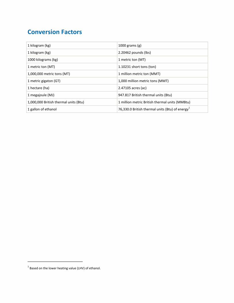
Conversion Factors
1 kilogram (kg) 1000 grams (g)
1 kilogram (kg) 2.20462 pounds (lbs)
1000 kilograms (kg) 1 metric ton (MT)
1 metric ton (MT) 1.10231 short tons (ton)
1,000,000 metric tons (MT) 1 million metric ton (MMT)
1 metric gigaton (GT) 1,000 million metric tons (MMT)
1 hectare (ha) 2.47105 acres (ac)
1 megajoule (MJ) 947.817 British thermal units (Btu)
1,000,000 British thermal units (Btu) 1 million metric British thermal units (MMBtu)
1 gallon of ethanol 76,330.0 British thermal units (Btu) of energy1
1 Based on the lower heating value (LHV) of ethanol.

blankpage
A Life-Cycle Analysis of the Greenhouse Gas Emissions of Corn-Based Ethanol
ICF 1 January 12, 2017
1. Introduction This chapter introduces the background for, the general approach for conducting the analyses described
in, and the organization of this report.
1.1. Background
Between 2004 and 2014, U.S. ethanol production, virtually all from corn starch, increased from 3.4 to
14.3 billion gallons per year. This increase in production was largely the result of two pieces of
legislation that mandated the nation’s supply of transportation fuel contain specified quantities of
renewable fuels (i.e. biofuels). Specifically, the Energy Policy Act of 2005 established the Renewable Fuel
Standard (RFS), which included a schedule of required biofuel use that started at 4 billion gallons in 2006
and rose to 7.5 billion gallons by 2012. Two years later, the Energy Independence and Security Act of
2007 replaced the RFS with the Revised Renewable Fuel Standard (RFS2). The RFS2 included a new
schedule of required biofuel use that began at 9 billion gallons in 2008 and ramped up to 36 billion
gallons in 2022. Corn ethanol’s mandate started at 9 billion gallons in 2008, gradually increased to 15
billion gallons in 2015, and was held constant at that level through 2022.
With the exception of ethanol produced in certain grandfathered refineries, a biofuel must have a life-
cycle greenhouse gas (GHG) profile at least 20 percent lower than that of the fossil fuel it replaces to
qualify as a renewable fuel under the RFS2. Earlier studies by Searchinger et al. (2008) and Fargione et
al. (2008) examined the effects of allocating billions of bushels of corn to ethanol production on supplies
of corn and other commodities going to domestic and world food and feed markets.2 These studies
proposed that domestic and world commodity prices would rise and farmers in the United States and
other regions would respond by bringing new lands into production. Bringing new land into commodity
production results typically in CO2 emissions and these emissions can be large if the former land use was
native grassland, wetland, or forest. The domestic and international land effects described above are
referred to as, respectively, “direct land-use change” and “indirect land-use change” (iLUC). GHG profiles
of corn ethanol date back to the early 1990s, but those done prior to 2007 did not account for emissions
related to iLUC. Searchinger et al. (2008) and Fargione et al. (2008) concluded that when emissions
related to iLUC are accounted for, corn ethanol has a higher GHG profile than gasoline. More recently,
researchers have reviewed the responses of farmers across the world to changes in corn demand. This
study draws on these new findings, including Bruce Babcock and Zabid Iqbal’s publication “Using Recent
Land Use Changes to Validate Land Use Change Models”. Babcock and Iqbal’s study confirmed that the
primary land-use change response by the world’s farmers during the period 2004–2012 was to use
2 The cap also reflected a practical constraint. For a various reasons, the ethanol content of gasoline sold in the Unites States for use in light trucks and automobiles is limited to 10 percent (a product called E10). This constraint is referred to as the “blend wall.” The blend wall presents a challenge to expanding ethanol consumption because virtually all gasoline now sold in the United States is E10. In 2015, for example, the United States consumed about 140.4 billion gallons of gasoline (https://www.eia.gov/tools/faqs/faq.cfm?id=23&t=10). The blend wall thus limited domestic consumption of ethanol in transportation fuel to a little over 14 billion gallons.
A Life-Cycle Analysis of the Greenhouse Gas Emissions of Corn-Based Ethanol
ICF 2 January 12, 2017
available land resources more efficiently rather than expanding land brought into production (Babcock
and Iqbal, 2014). Farmers in Brazil, India, and China have increased double cropping, reduced
unharvested planted area, reduced fallow land, and reduced temporary pasture in order to expand
production.
The RFS2 directed the U.S. Environmental Protection Agency (EPA) to do a full life-cycle analysis (LCA) of
greenhouse gas (GHG) emissions associated with the production of corn ethanol (as well as other
biofuels) and explicitly specified that emissions related to iLUC be included. In 2010, EPA released this
LCA as part of its Regulatory Impact Analysis (RIA) of the RFS2. The EPA RIA developed projections
through 2022 of the GHG emissions associated with 11 specific emission categories that, conceptually,
capture the full range of direct and indirect GHG emissions associated with corn-ethanol production and
combustion (i.e., from corn field to tailpipe). These emission categories include:
1. Domestic farm inputs and fertilizer N2O
2. Domestic land-use change
3. Domestic rice methane3
4. Domestic livestock4
5. International land-use change
6. International farm inputs and fertilizer N2O
7. International rice methane
8. International livestock
9. Fuel and feedstock transport
10. Fuel production
11. Tailpipe
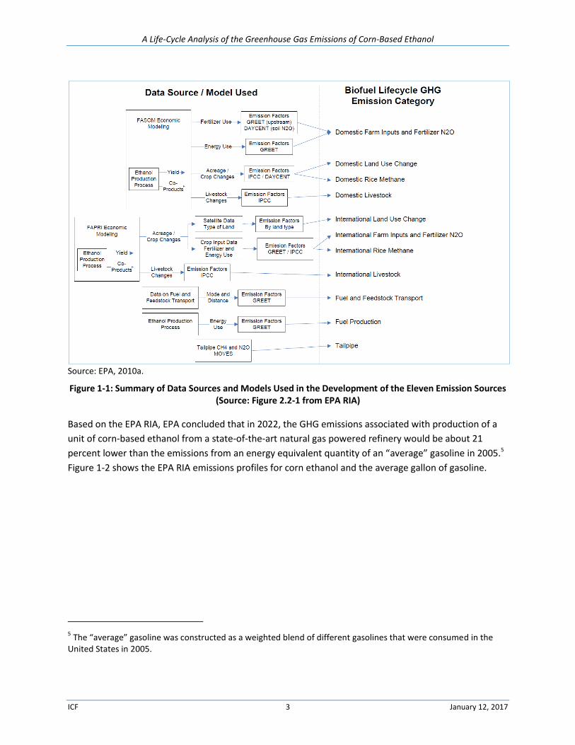
Figure 1-1 presents these emission categories and the data sources and models that EPA used to
estimate their GHG emissions. EPA evaluated the emissions and energy use associated with each
emission category and the upstream components.
3 Domestic rice methane is included to account for changes in land-use emissions based on the increased demand for biofuels and change in domestic rice acreage.
4 Domestic livestock is included to account for the change in livestock production as costs for feed changes due to corn ethanol
production.
A Life-Cycle Analysis of the Greenhouse Gas Emissions of Corn-Based Ethanol
ICF 3 January 12, 2017
Source: EPA, 2010a.
Figure 1-1: Summary of Data Sources and Models Used in the Development of the Eleven Emission Sources (Source: Figure 2.2-1 from EPA RIA)
Based on the EPA RIA, EPA concluded that in 2022, the GHG emissions associated with production of a
unit of corn-based ethanol from a state-of-the-art natural gas powered refinery would be about 21
percent lower than the emissions from an energy equivalent quantity of an “average” gasoline in 2005.5
Figure 1-2 shows the EPA RIA emissions profiles for corn ethanol and the average gallon of gasoline.
5 The “average” gasoline was constructed as a weighted blend of different gasolines that were consumed in the United States in 2005.
A Life-Cycle Analysis of the Greenhouse Gas Emissions of Corn-Based Ethanol
ICF 4 January 12, 2017
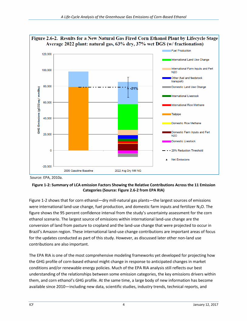
Source: EPA, 2010a.
Figure 1-2: Summary of LCA emission Factors Showing the Relative Contributions Across the 11 Emission Categories (Source: Figure 2.6-2 from EPA RIA)
Figure 1-2 shows that for corn ethanol—dry mill-natural gas plants—the largest sources of emissions
were international land-use change, fuel production, and domestic farm inputs and fertilizer N2O. The
figure shows the 95 percent confidence interval from the study’s uncertainty assessment for the corn
ethanol scenario. The largest source of emissions within international land-use change are the
conversion of land from pasture to cropland and the land-use change that were projected to occur in
Brazil’s Amazon region. These international land-use change contributions are important areas of focus
for the updates conducted as part of this study. However, as discussed later other non-land use
contributions are also important.
The EPA RIA is one of the most comprehensive modeling frameworks yet developed for projecting how
the GHG profile of corn-based ethanol might change in response to anticipated changes in market
conditions and/or renewable energy policies. Much of the EPA RIA analysis still reflects our best
understanding of the relationships between some emission categories, the key emissions drivers within
them, and corn ethanol’s GHG profile. At the same time, a large body of new information has become
available since 2010—including new data, scientific studies, industry trends, technical reports, and
A Life-Cycle Analysis of the Greenhouse Gas Emissions of Corn-Based Ethanol
ICF 5 January 12, 2017
updated emissions coefficients—that indicates that for many of the emission categories in the EPA RIA,
the actual emissions pathways that have developed since 2010 differ significantly from those projected
in the EPA RIA. The primary purpose of this report is to consider a more complete set of information
now available related to the life-cycle emissions for corn-based ethanol and based on this information,
assess its current (i.e., in 2014) GHG emissions profile.
This report also develops two projected emissions profiles for corn ethanol in 2022 (the last year of the
RFS2). Starting with the current emissions profile, the first projection, labeled the business-as-usual
(BAU) scenario, assumes that recent trends observed in corn inputs and per-acre yields, refinery
technologies, vehicle fleets, and other factors continue through 2022. The continuation of these trends
has implications for the path that GHG emissions attributable to corn ethanol production will follow
over the next few years. The second projection, labeled the Building-Blocks scenario, adds to the BAU
the assumption that refineries adopt a set of currently available GHG reducing technologies and
practices in corn production, transportation, and co-products. The Building-Blocks scenario can be
viewed as a best-case assessment of corn ethanol’s potential to mitigate GHG emissions given currently
available technologies and production practices.
1.2. General Approach
Since 2010, the EPA RIA’s estimated GHG mitigation value for corn ethanol, 21 percent lower emissions
than an energy equivalent quantity of gasoline, has dominated academic, industry, and policy
discussions of GHG issues related to renewable transportation fuels, as well as the design of federal
renewable fuels policy (specifically, the RFS2). For these reasons, the structure the LCA developed in this
report is designed so that comparisons of its results with those in the EPA RIA are relatively
straightforward. For example, to match boundary conditions and emissions coverage, this study employs
the same 11 emission categories that make up the EPA RIA. Due to the EPA RIA’s comprehensive
coverage of GHG emissions, both in aggregate and within each category, it is generally straightforward
to assess where new information indicates that current emissions differ from the paths projected in
2010, as well as what the magnitudes and directions of the differences are.
Another structural similarity that facilitates comparisons between the LCA developed here and that in
the RIA is a focus on the increase in corn ethanol production attributable to the RFS2 in assessing corn
ethanol’s GHG profile. This results in an emphasis on the relationships that currently exist between the
11 emission categories, the key GHG drivers within them, and ethanol’s GHG profile. Based on a 2007
projection of ethanol production (i.e., before the RFS2) done by the Department of Energy’s Energy
Information Agency (EIA) without an RFS in place and the 15 billion gallon cap on corn ethanol in the
RFS2, EPA projected that the RFS2 would increase corn ethanol production by 3.03 billion gallons in
2014 and 2.6 billion gallons in 2022 over the baseline EIA projection.6 We used the 3.03 billion gallon
increase in ethanol production to assess the contribution of most of the emission categories in the
6 In January of 2007, total ethanol production capacity in place and under construction was 11.6 billion gallons (RFA, 2007).
A Life-Cycle Analysis of the Greenhouse Gas Emissions of Corn-Based Ethanol
ICF 6 January 12, 2017
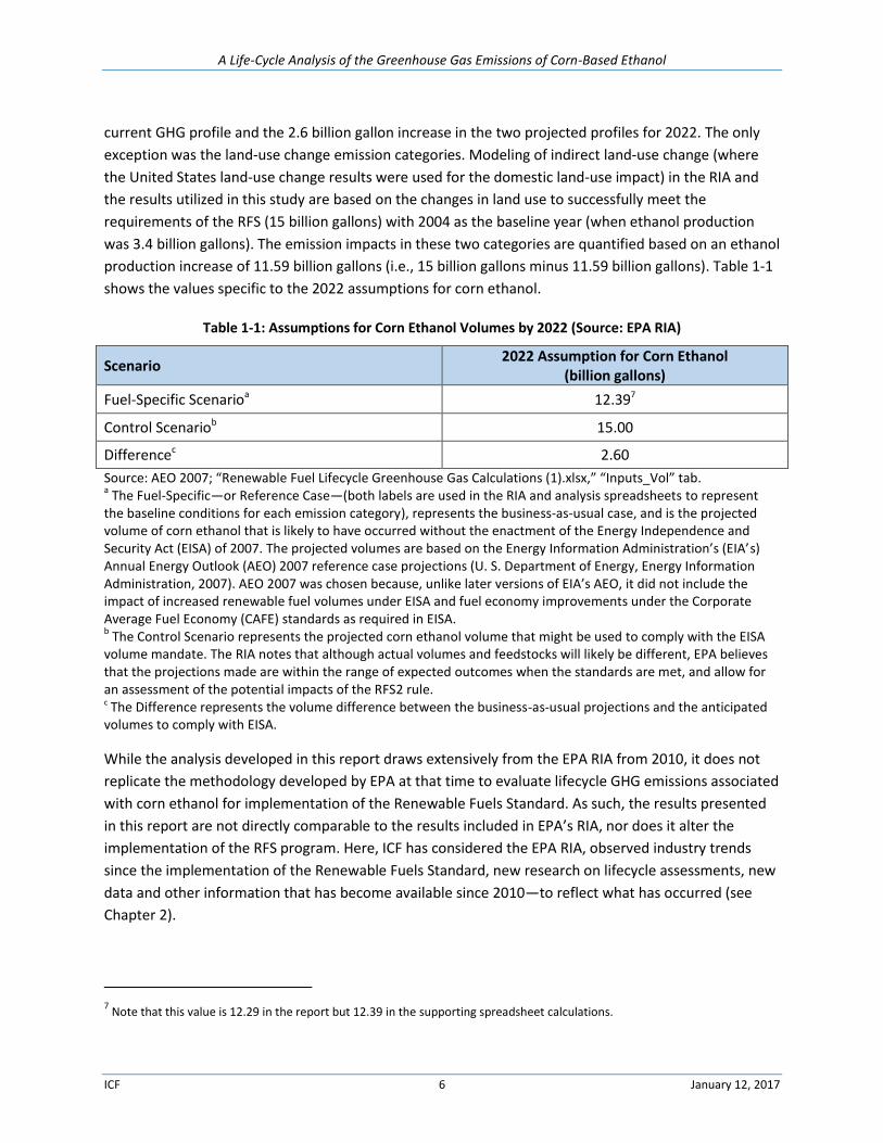
current GHG profile and the 2.6 billion gallon increase in the two projected profiles for 2022. The only
exception was the land-use change emission categories. Modeling of indirect land-use change (where
the United States land-use change results were used for the domestic land-use impact) in the RIA and
the results utilized in this study are based on the changes in land use to successfully meet the
requirements of the RFS (15 billion gallons) with 2004 as the baseline year (when ethanol production
was 3.4 billion gallons). The emission impacts in these two categories are quantified based on an ethanol
production increase of 11.59 billion gallons (i.e., 15 billion gallons minus 11.59 billion gallons). Table 1-1
shows the values specific to the 2022 assumptions for corn ethanol.
Table 1-1: Assumptions for Corn Ethanol Volumes by 2022 (Source: EPA RIA)
Scenario 2022 Assumption for Corn Ethanol
(billion gallons)
Fuel-Specific Scenarioa 12.397
Control Scenariob 15.00
Differencec 2.60
Source: AEO 2007; “Renewable Fuel Lifecycle Greenhouse Gas Calculations (1).xlsx,” “Inputs_Vol” tab. a The Fuel-Specific—or Reference Case—(both labels are used in the RIA and analysis spreadsheets to represent
the baseline conditions for each emission category), represents the business-as-usual case, and is the projected volume of corn ethanol that is likely to have occurred without the enactment of the Energy Independence and Security Act (EISA) of 2007. The projected volumes are based on the Energy Information Administration’s (EIA’s) Annual Energy Outlook (AEO) 2007 reference case projections (U. S. Department of Energy, Energy Information Administration, 2007). AEO 2007 was chosen because, unlike later versions of EIA’s AEO, it did not include the impact of increased renewable fuel volumes under EISA and fuel economy improvements under the Corporate Average Fuel Economy (CAFE) standards as required in EISA. b The Control Scenario represents the projected corn ethanol volume that might be used to comply with the EISA
volume mandate. The RIA notes that although actual volumes and feedstocks will likely be different, EPA believes that the projections made are within the range of expected outcomes when the standards are met, and allow for an assessment of the potential impacts of the RFS2 rule. c The Difference represents the volume difference between the business-as-usual projections and the anticipated
volumes to comply with EISA.
While the analysis developed in this report draws extensively from the EPA RIA from 2010, it does not
replicate the methodology developed by EPA at that time to evaluate lifecycle GHG emissions associated
with corn ethanol for implementation of the Renewable Fuels Standard. As such, the results presented
in this report are not directly comparable to the results included in EPA’s RIA, nor does it alter the
implementation of the RFS program. Here, ICF has considered the EPA RIA, observed industry trends
since the implementation of the Renewable Fuels Standard, new research on lifecycle assessments, new
data and other information that has become available since 2010—to reflect what has occurred (see
Chapter 2).
7 Note that this value is 12.29 in the report but 12.39 in the supporting spreadsheet calculations.
A Life-Cycle Analysis of the Greenhouse Gas Emissions of Corn-Based Ethanol
ICF 7 January 12, 2017
New information accounted for in this assessment includes new values that have been developed since
2010 for many of the GHG emissions coefficients and conversion factors used in the RIA. These
coefficients and factors are used to assign GHG emissions values to specific changes in economic
activity, input use, land management practices, and output levels. In general, updated values for specific
emissions coefficients and factors are discussed in the sections where they are applicable. One set of
updated conversion factors, however, applies across emission categories and is discussed below.
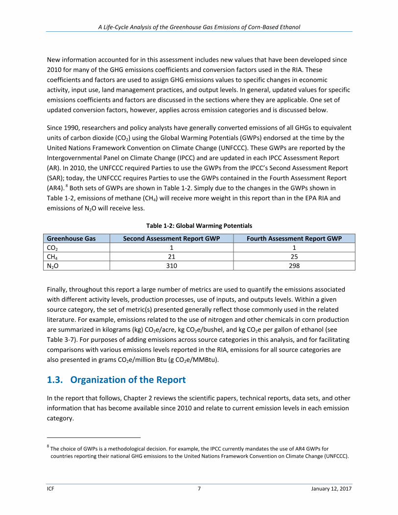
Since 1990, researchers and policy analysts have generally converted emissions of all GHGs to equivalent
units of carbon dioxide (CO2) using the Global Warming Potentials (GWPs) endorsed at the time by the
United Nations Framework Convention on Climate Change (UNFCCC). These GWPs are reported by the
Intergovernmental Panel on Climate Change (IPCC) and are updated in each IPCC Assessment Report
(AR). In 2010, the UNFCCC required Parties to use the GWPs from the IPCC’s Second Assessment Report
(SAR); today, the UNFCCC requires Parties to use the GWPs contained in the Fourth Assessment Report
(AR4). 8 Both sets of GWPs are shown in Table 1-2. Simply due to the changes in the GWPs shown in
Table 1-2, emissions of methane (CH4) will receive more weight in this report than in the EPA RIA and
emissions of N2O will receive less.
Table 1-2: Global Warming Potentials
Greenhouse Gas Second Assessment Report GWP Fourth Assessment Report GWP
CO2 1 1
CH4 21 25
N2O 310 298
Finally, throughout this report a large number of metrics are used to quantify the emissions associated
with different activity levels, production processes, use of inputs, and outputs levels. Within a given
source category, the set of metric(s) presented generally reflect those commonly used in the related
literature. For example, emissions related to the use of nitrogen and other chemicals in corn production
are summarized in kilograms (kg) CO2e/acre, kg CO2e/bushel, and kg CO2e per gallon of ethanol (see
Table 3-7). For purposes of adding emissions across source categories in this analysis, and for facilitating
comparisons with various emissions levels reported in the RIA, emissions for all source categories are
also presented in grams CO2e/million Btu (g CO2e/MMBtu).
1.3. Organization of the Report
In the report that follows, Chapter 2 reviews the scientific papers, technical reports, data sets, and other
information that has become available since 2010 and relate to current emission levels in each emission
category.
8 The choice of GWPs is a methodological decision. For example, the IPCC currently mandates the use of AR4 GWPs for
countries reporting their national GHG emissions to the United Nations Framework Convention on Climate Change (UNFCCC).
A Life-Cycle Analysis of the Greenhouse Gas Emissions of Corn-Based Ethanol
ICF 8 January 12, 2017
Chapter 3 develops current GHG emission values for each emission category included in the EPA RIA
based on the literature review. Chapter 3 considers each emission category separately. For each
emission category, the section includes a summary of the methods, data sources, and emissions
projection developed in the EPA RIA, describes the methods ICF used to quantify the contribution to
corn ethanol’s current GHG profile attributable to that category, and quantifies that contribution.
Based on the current GHG emissions profile of corn ethanol developed in Chapter 3, Chapter 4 develops
two projected profiles for corn ethanol in 2022. The first projection considers a continuation through
2022 of observable trends in corn yields (per acre), process fuel switching toward natural gas, and fuel
efficiency in trucking. The second projection adds a number of changes refineries could make in their
value chain to further reduce the GHG intensity of corn ethanol. These changes include contracting with
farmers to reduce tillage and manage nitrogen applications, switch to biomass as a process fuel, and
locating confined livestock operations in close proximity to refineries.
1.4. References: Introduction
Babcock, B.A. and Iqbal, Z., 2014. “Using Recent Land Use Changes to Validate Land Use Change Models”. Staff Report 14-SR 109. Center for Agricultural and Rural Development: Iowa State University. http://www.card.iastate.edu/publications/dbs/pdffiles/14sr109.pdf
EPA. (2010, February). U.S. Environmental Protection Agency: Renewable Fuel Standard (RFS2) Regulatory Impact Analysis. Retrieved from http://www.epa.gov/oms/renewablefuels/420r10006.pdf
Fargione, J., J. Hill, D. Tilman, S. Polasky, and P. Hawthorne. 2008. “Land Clearing and the Biofuel Carbon Debt.” Science. Vol 319. 29 February: pp 1235-1238.
Renewable Fuels Association (RFA). 2007. Ethanol Industry Outlook, 2007: Building New Horizons. Available at: http://ethanolrfa.org/wp-content/uploads/2015/09/RFA_Outlook_2007.pdf
Searchinger, T., R. Heimlich, R.A. Houghton, F. Dong, A. Elobeid, J. Fabiosa, S. Tokgoz, D. Hayes, and T. Yu. 2008. “Use of Cropland for Biofuels Increases Greenhouse Gases Through Emissions from Land-Use Change.” Science. Vol 319. 29 February: pp 1238-1240.
U. S. Department of Energy, Energy Information Administration. (2007, February). Annual Energy Outlook. Retrieved from http://tonto.eia.doe.gov/ftproot/forecasting/0383(2007).pdf
A Life-Cycle Analysis of the Greenhouse Gas Emissions of Corn-Based Ethanol
ICF 9 January 12, 2017
2. Review of the Scientific Papers, Technical Reports, Data Sets, and Other Information that have Become Available Since 2010 and Relate to Current Emissions Levels in Each Emissions Category This chapter reviews and synthesizes the scientific papers, technical reports, data sets, and other
information in the peer-reviewed and credible non-peer-reviewed literature that have become available
since 2010 and relate to current emissions levels in the 11 source categories included in EPA’s
Renewable Fuel Standard Program (RFS2) Regulatory Impact Analysis (RIA). The review is organized by
emission category with the exception of the domestic livestock with international livestock categories,
which are dealt with in one section. For each emission category, a summary of the scientific papers,
technical reports, data sets, and other information that has become available since 2010 is provided.
Where applicable, information, data, and emission factors from the more recent literature is compared
to corresponding information and data used in the RIA.9 In addition, key issues identified in the available
literature are summarized.
The remainder of this chapter is organized as follows:
1. Domestic farm inputs and fertilizer N2O
2. Domestic land-use change
3. Domestic rice methane
4. Domestic and international livestock
5. International land-use change
6. International farm inputs and fertilizer N2O
7. International rice methane
8. Fuel and feedstock transport
9. Fuel production
10. Tailpipe
2.1. Domestic Farm Inputs and Fertilizer N2O
The domestic farm inputs evaluated in the RIA include fertilizers, herbicides, pesticides, and on-site fuel
use. The fertilizers evaluated included nitrogen, phosphorous, potash, and lime. Representative
herbicides and pesticides were also included. On-site fuels included diesel, gasoline, natural gas, and
electricity. N2O emissions due to application of synthetic fertilizers were also quantified.
9 Many of the inputs for the existing EPA emission estimates come from established data sources (e.g., the emission factors included in GREET) and other model outputs (e.g., FASOM, FAPRI, MOVES). We reviewed updated output datasets including emission factors from more recent versions of these models. For example, Argonne National Laboratory’s GREET and Carbon Calculator for Land Use Change from Biofuels Production (CCLUB) models were updated in 2015, so ICF was able to readily compare any updated emission factors against those used for the RIA.
A Life-Cycle Analysis of the Greenhouse Gas Emissions of Corn-Based Ethanol
ICF 10 January 12, 2017
The RIA uses estimates of domestic agricultural inputs for fertilizer, pesticides, and energy use from the
Forestry and Agriculture Sector Optimization Model (FASOM) output. Since the release of the RFS2 RIA,
additional empirical data are available to validate and/or update those inputs used in the analysis. For
example, the U.S. Department of Agriculture’s (USDA) National Agricultural Statistics Service (NASS)
reports much of these data under the Agricultural Chemical Use Program.
2.1.1. Domestic Farm Chemical Use
The NASS Agricultural Chemical Use Program is USDA’s official source of statistics about on-farm
chemical use and pest management practices.10 Since 1990, NASS has surveyed U.S. farmers to collect
information on the chemical ingredients they apply to agricultural commodities through fertilizers and
pesticides. On a rotating basis, the program currently includes fruits; vegetables; major field crops such
as cotton, corn, potatoes, soybeans, and wheat; and nursery and floriculture crops.
Each survey focuses on the top-producing states that together account for the majority of U.S. acres or
production of the surveyed commodity. Data are available at the state level for all surveyed states, as
well as at a multi-state level including all surveyed states. Data items published include, but are not
limited to:
Percentage acreage treated, number of applications, rates of application, and total amounts applied
of the primary macronutrients nitrogen (N), phosphate (P2O5), and potash (K2O) as well as (since
2005) the secondary macronutrient sulfur (S). Available annually for field crops.
Percentage acreage or production treated, number of applications, rates of application, and total
amounts applied of the individual active ingredients composing all registered pesticides used. Active
ingredients are classified as herbicides, fungicides, insecticides, or other (regulators, desiccants,
etc.), according to the pesticide product classification. Rates and amounts applied are published in
the acid or metallic equivalent, as applicable. Selected items available for all commodity programs.
2.1.2. Domestic Farm Energy Use
Periodically, USDA produces an updated inventory of GHG emissions and carbon storage for the
agriculture and forestry sectors. These reports are consistent with the annual emissions reporting done
by EPA, but provide an enhanced view of the data regionally and by land use.
The report is prepared with contributions from the USDA Agricultural Research Service, USDA Forest
Service, USDA Natural Resources Conservation Service, USDA Office of Energy Policy and New Uses,
USDA Climate Change Program Office, U.S. Environmental Protection Agency (EPA), and researchers at
Colorado State University. The estimates in the USDA GHG Inventory are consistent with those
published by the EPA in the official Inventory of U.S. Greenhouse Gas Emissions and Sinks. The last USDA
10 More information on the program, and access to the data Chemical Use data from the NASS Quick Stats database is available online at: http://www.nass.usda.gov/Surveys/Guide_to_NASS_Surveys/Chemical_Use/
A Life-Cycle Analysis of the Greenhouse Gas Emissions of Corn-Based Ethanol
ICF 11 January 12, 2017
GHG inventory was published in September 2016. Chapter 5 of the USDA Agriculture and Forestry
Greenhouse Gas Inventory: 1990–2013 provides information on energy use in agriculture (USDA, 2016a).
Empirical data with which to validate and/or update those inputs used (and emissions estimated) in the
RFS2 RIA analysis is available from the underlying data source (and emission factors) used in the
inventory.
Estimates of CO2 from agricultural operations are based on energy expense data from
the Agricultural Resource Management Survey (ARMS) conducted by the National
Agricultural Statistics Service (NASS) of the USDA. The ARMS collects information on
farm production expenditures, including expenditures on diesel fuel, gasoline, LP gas,
natural gas, and electricity... NASS also collects data on price per gallon paid by farmers
for gasoline, diesel, and LP gas... Energy expenditures are divided by fuel prices to
approximate gallons of fuel consumed by farmers. Gallons of gasoline, diesel, and LP gas
are then converted to Btu based on the heating value of each of the fuels. The individual
farm data are aggregated by state, and the state data are divided into 10 production
regions, allowing fuel consumption to be estimated at the national and regional levels.
Farm consumption estimates for electricity and natural gas are also approximated by
dividing prices into expenditures. Since electricity and natural gas prices are not collected
by NASS, we use data from the Energy Information Administration (EIA) that reports
average prices by state… NASS regional prices were derived by aggregating the EIA state
data into NASS production regions. (USDA, 2011)
2.1.3. Domestic Farm Nitrogen Application
As indicated in the recent literature (see Table 2-1), N application has increased from 137 to 143 pounds
per acre from 2005 to 2010. However, yield per acre has increased during the same period, thereby
resulting in a net decrease in N application per crop yield. In particular, as The Fertilizer Institute states:
Between 1980 and 2014, U.S. farmers more than doubled corn production using only
slightly more fertilizer nutrients than were used in 1980. This analysis is based on
fertilizer application rate and corn production and acreage data reported by the U.S.
Department of Agriculture’s (USDA) National Agricultural Statistics Service (NASS).
Specifically, in 1980, farmers grew 6.64 billion bushels of corn using 3.2 pounds of
nutrients (nitrogen, phosphorus and potassium) for each bushel and in 2014 they grew
14.22 billion bushels using less than 1.6 pounds of nutrients per bushel produced. In
total, this represents an 114 percent increase in production using only 4.5 percent more
nutrients during that same timeframe.
Between 2010 and 2014 there was a slight decrease in fertilizer per bushel (i.e., from 1.63 to 1.56
pounds of N per bushel) (The Fertilizer Institute, 2016). This decrease in fertilizer application, combined
with the direct change in acres, could reduce the impact of domestic nitrogen application.
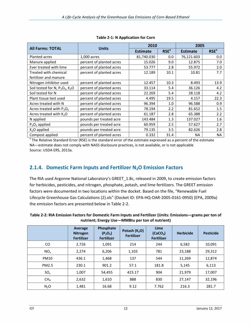
A Life-Cycle Analysis of the Greenhouse Gas Emissions of Corn-Based Ethanol
ICF 12 January 12, 2017
Table 2-1: N Application for Corn
All Farms: TOTAL Units 2010 2005
Estimate RSEa Estimate RSEa Planted acres 1,000 acres 81,740.030 0.0 76,121.603 0.0
Manure applied percent of planted acres 15.026 9.0 12.875 7.0
Ever treated with lime percent of planted acres 53.777 2.8 55.972 2.0
Treated with chemical fertilizer and manure
percent of planted acres 12.189 10.1 10.81 7.7
Nitrogen inhibitor used percent of planted acres 12.457 10.3 8.493 13.9
Soil tested for N, P2O5, K2O percent of planted acres 33.114 5.4 36.126 4.2
Soil tested for N percent of planted acres 22.269 5.4 28.118 4.2
Plant tissue test used percent of planted acres 4.495 19.5 4.157 22.3
Acres treated with N percent of planted acres 96.394 1.0 96.588 0.9
Acres treated with P2O5 percent of planted acres 78.194 2.2 81.652 1.5
Acres treated with K2O percent of planted acres 61.187 2.8 65.388 2.2
N applied pounds per treated acre 143.484 1.3 137.027 1.6
P2O5 applied pounds per treated acre 60.959 2.5 57.627 2.7
K2O applied pounds per treated acre 79.135 3.5 82.626 2.8
Compost applied percent of planted acres 0.332 31.4 NA NA a The Relative Standard Error (RSE) is the standard error of the estimate expressed as a percent of the estimate
NA—estimate does not comply with NASS disclosure practices, is not available, or is not applicable Source: USDA ERS, 2013a.
2.1.4. Domestic Farm Inputs and Fertilizer N2O Emission Factors
The RIA used Argonne National Laboratory’s GREET_1.8c, released in 2009, to create emission factors
for herbicides, pesticides, and nitrogen, phosphate, potash, and lime fertilizers. The GREET emission
factors were documented in two locations within the docket. Based on the file, “Renewable Fuel
Lifecycle Greenhouse Gas Calculations (2).xls” (Docket ID: EPA-HQ-OAR-2005-0161-0950) (EPA, 2009a)
the emission factors are presented below in Table 2-2.
Table 2-2: RIA Emission Factors for Domestic Farm Inputs and Fertilizer (Units: Emissions—grams per ton of nutrient; Energy Use—MMBtu per ton of nutrient)
Average Nitrogen Fertilizer
Phosphate (P2O5)
Fertilizer
Potash (K2O) Fertilizer
Lime (CaCO3)
Fertilizer Herbicide Pesticide
CO 2,726 1,091 214 244 6,582 10,091
NOx 2,274 6,206 1,103 781 23,188 29,312
PM10 436.1 1,468 137 544 11,269 12,874
PM2.5 230.1 901.2 57.1 181.8 5,145 6,113
SOx 1,007 54,455 423.17 904 21,979 17,007
CH4 2,632 1,610 888 830 27,147 32,196
N2O 1,481 16.68 9.12 7.762 216.3 281.7
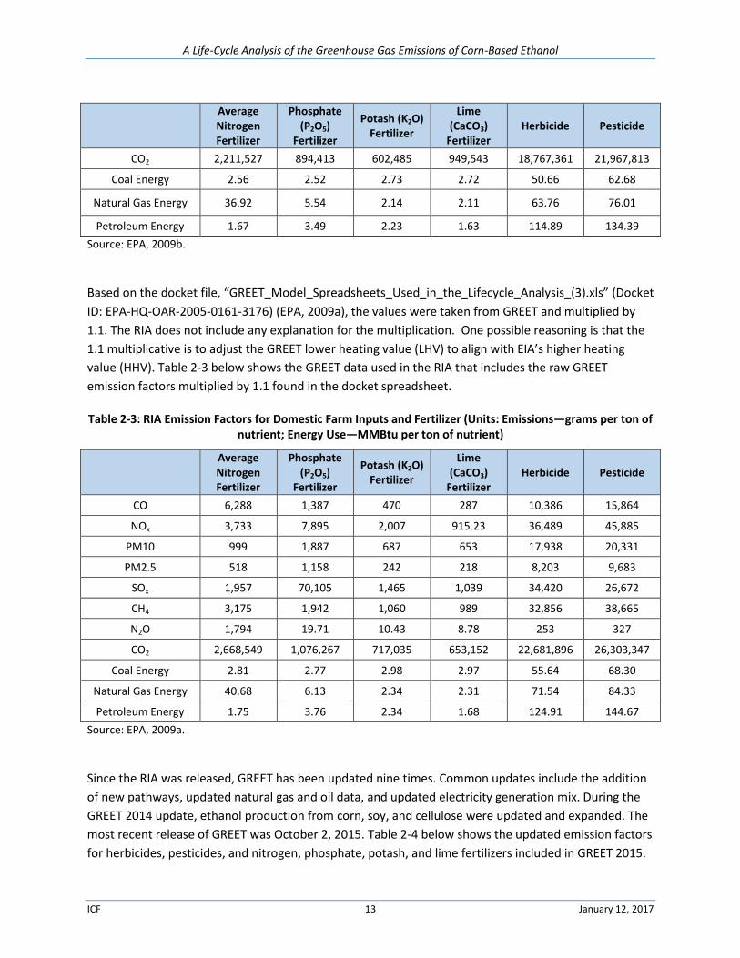
A Life-Cycle Analysis of the Greenhouse Gas Emissions of Corn-Based Ethanol
ICF 13 January 12, 2017
Average Nitrogen Fertilizer
Phosphate (P2O5)
Fertilizer
Potash (K2O) Fertilizer
Lime (CaCO3)
Fertilizer Herbicide Pesticide
CO2 2,211,527 894,413 602,485 949,543 18,767,361 21,967,813
Coal Energy 2.56 2.52 2.73 2.72 50.66 62.68
Natural Gas Energy 36.92 5.54 2.14 2.11 63.76 76.01
Petroleum Energy 1.67 3.49 2.23 1.63 114.89 134.39
Source: EPA, 2009b.
Based on the docket file, “GREET_Model_Spreadsheets_Used_in_the_Lifecycle_Analysis_(3).xls” (Docket
ID: EPA-HQ-OAR-2005-0161-3176) (EPA, 2009a), the values were taken from GREET and multiplied by
1.1. The RIA does not include any explanation for the multiplication. One possible reasoning is that the
1.1 multiplicative is to adjust the GREET lower heating value (LHV) to align with EIA’s higher heating
value (HHV). Table 2-3 below shows the GREET data used in the RIA that includes the raw GREET
emission factors multiplied by 1.1 found in the docket spreadsheet.
Table 2-3: RIA Emission Factors for Domestic Farm Inputs and Fertilizer (Units: Emissions—grams per ton of nutrient; Energy Use—MMBtu per ton of nutrient)
Average Nitrogen Fertilizer
Phosphate (P2O5)
Fertilizer
Potash (K2O) Fertilizer
Lime (CaCO3)
Fertilizer Herbicide Pesticide
CO 6,288 1,387 470 287 10,386 15,864
NOx 3,733 7,895 2,007 915.23 36,489 45,885
PM10 999 1,887 687 653 17,938 20,331
PM2.5 518 1,158 242 218 8,203 9,683
SOx 1,957 70,105 1,465 1,039 34,420 26,672
CH4 3,175 1,942 1,060 989 32,856 38,665
N2O 1,794 19.71 10.43 8.78 253 327
CO2 2,668,549 1,076,267 717,035 653,152 22,681,896 26,303,347
Coal Energy 2.81 2.77 2.98 2.97 55.64 68.30
Natural Gas Energy 40.68 6.13 2.34 2.31 71.54 84.33
Petroleum Energy 1.75 3.76 2.34 1.68 124.91 144.67
Source: EPA, 2009a.
Since the RIA was released, GREET has been updated nine times. Common updates include the addition
of new pathways, updated natural gas and oil data, and updated electricity generation mix. During the
GREET 2014 update, ethanol production from corn, soy, and cellulose were updated and expanded. The
most recent release of GREET was October 2, 2015. Table 2-4 below shows the updated emission factors
for herbicides, pesticides, and nitrogen, phosphate, potash, and lime fertilizers included in GREET 2015.
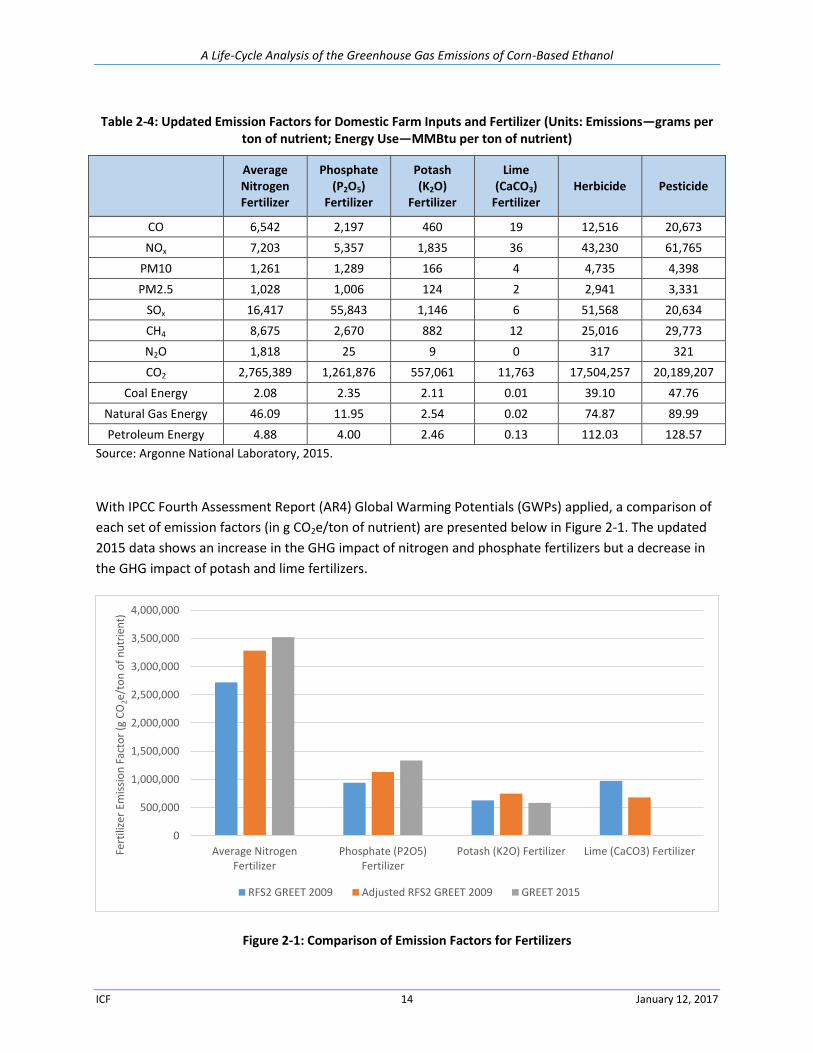
A Life-Cycle Analysis of the Greenhouse Gas Emissions of Corn-Based Ethanol
ICF 14 January 12, 2017
Table 2-4: Updated Emission Factors for Domestic Farm Inputs and Fertilizer (Units: Emissions—grams per ton of nutrient; Energy Use—MMBtu per ton of nutrient)
Average Nitrogen Fertilizer
Phosphate (P2O5)
Fertilizer
Potash (K2O)
Fertilizer
Lime (CaCO3)
Fertilizer Herbicide Pesticide
CO 6,542 2,197 460 19 12,516 20,673
NOx 7,203 5,357 1,835 36 43,230 61,765
PM10 1,261 1,289 166 4 4,735 4,398
PM2.5 1,028 1,006 124 2 2,941 3,331
SOx 16,417 55,843 1,146 6 51,568 20,634
CH4 8,675 2,670 882 12 25,016 29,773
N2O 1,818 25 9 0 317 321
CO2 2,765,389 1,261,876 557,061 11,763 17,504,257 20,189,207
Coal Energy 2.08 2.35 2.11 0.01 39.10 47.76
Natural Gas Energy 46.09 11.95 2.54 0.02 74.87 89.99
Petroleum Energy 4.88 4.00 2.46 0.13 112.03 128.57
Source: Argonne National Laboratory, 2015.
With IPCC Fourth Assessment Report (AR4) Global Warming Potentials (GWPs) applied, a comparison of
each set of emission factors (in g CO2e/ton of nutrient) are presented below in Figure 2-1. The updated
2015 data shows an increase in the GHG impact of nitrogen and phosphate fertilizers but a decrease in
the GHG impact of potash and lime fertilizers.
Figure 2-1: Comparison of Emission Factors for Fertilizers
0
500,000
1,000,000
1,500,000
2,000,000
2,500,000
3,000,000
3,500,000
4,000,000
Average NitrogenFertilizer
Phosphate (P2O5)Fertilizer
Potash (K2O) Fertilizer Lime (CaCO3) FertilizerFert
ilize
r Em
issi
on
Fac
tor
(g C
O2e
/to
n o
f n
utr
ien
t)
RFS2 GREET 2009 Adjusted RFS2 GREET 2009 GREET 2015
A Life-Cycle Analysis of the Greenhouse Gas Emissions of Corn-Based Ethanol
ICF 15 January 12, 2017
As the tables show, there are significant differences in emissions and energy use between GREET1_2009
and GREET1_2015 for nitrogen fertilizer and lime.
For nitrogen fertilizer, between 2009 and 2015, Argonne adjusted energy use for nitrogen fertilizer
manufacturing by increasing natural gas use across all nitrogen fertilizer types. For lime, energy use and
emissions are significantly reduced from GREET_2009 to GREET_2015. The changes result from
Argonne’s correction of using crushed limestone in GREET_2015 from using lime in GREET_2009.
2.1.5. Domestic Farm Input and Fertilizer N2O Management Practices
While the RIA includes comprehensive information on emission factors, it does not include the recent
literature discussing an increase in crop and nutrient management strategies. These strategies have the
potential to reduce the emissions from agriculture production, which could have a noticeable impact on
domestic farm input and fertilizer N2O emission calculations such as for the corn ethanol LCA. Two of the
most common of these strategies are use of nitrification inhibitors and precision agriculture. USDA
statistics already reflect the effects of precision agriculture through the reduced fertilizer use per bushel
of corn harvest, however use of nitrification inhibitors is not reflected in estimation of N2O emissions.
Nitrification inhibitors work by slowing the nitrification process when nitrogen-based fertilizer is applied
to crops, which allows for an increase in nitrogen use efficiency. Inhibitors can be mixed into fertilizers
or applied separately, and they give crops access to a larger percentage of applied fertilizer. This
increased access to applied nitrogen improves the nitrogen use and reduces the nitrogen loss from
crops, which decreases the resulting emissions from applied nitrogen-based fertilizers. More specifically,
as Trenkel (2010) explains in his comprehensive paper on enhancing nutrient use efficiency in
agriculture through slow- and controlled-release and stabilized fertilizers, the Association of American
Plant Food Control Officials (AAPFCO) defines a nitrification inhibitor as “a substance that inhibits the
biological oxidation of ammoniacal-N to nitrate-N” (Trenkel, 2010). Maintaining the nitrogen in its
ammonium form longer gives crops a more prolonged chance for nitrogen-uptake, therefore using the
applied nitrogen more effectively and reducing emissions through nitrogen loss.
Precision agriculture refers to crop strategies that use field-specific data to optimize outputs. As
Schimmelpfennig and Ebel (2011) describe in their paper on the recent adoption of precision agriculture,
the term precision agriculture is used to designate crop practices that use “information gathered during
field operations, from planting to harvest, to calibrate the application of inputs and economize on fuel
use.” These practices include GPS- and sensor-based mapping systems that regulate the application rate
of inputs such as fertilizers and eliminate the potential for overlapping application on corners and
irregular fields. Systems that regulate and optimize the application rate are typically called variable rate
technology (VRT) or variable rate application (VRA), while systems that reduce or eliminate overlap in
application are typically called swath control.
Studies released since the implementation of RFS2 show that use of inhibitors on crops can reduce
emissions around 20 to 60 percent, depending on factors such as timing of application and soil moisture
(Halvorson, 2014; Thapa et al., 2015). In a slightly more modest range, recent literature indicates that
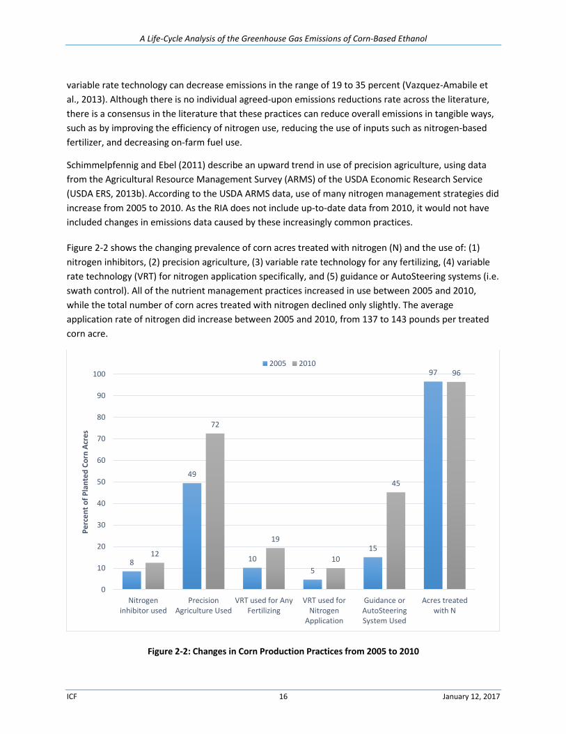
A Life-Cycle Analysis of the Greenhouse Gas Emissions of Corn-Based Ethanol
ICF 16 January 12, 2017
variable rate technology can decrease emissions in the range of 19 to 35 percent (Vazquez-Amabile et
al., 2013). Although there is no individual agreed-upon emissions reductions rate across the literature,
there is a consensus in the literature that these practices can reduce overall emissions in tangible ways,
such as by improving the efficiency of nitrogen use, reducing the use of inputs such as nitrogen-based
fertilizer, and decreasing on-farm fuel use.
Schimmelpfennig and Ebel (2011) describe an upward trend in use of precision agriculture, using data
from the Agricultural Resource Management Survey (ARMS) of the USDA Economic Research Service
(USDA ERS, 2013b). According to the USDA ARMS data, use of many nitrogen management strategies did
increase from 2005 to 2010. As the RIA does not include up-to-date data from 2010, it would not have
included changes in emissions data caused by these increasingly common practices.
Figure 2-2 shows the changing prevalence of corn acres treated with nitrogen (N) and the use of: (1)
nitrogen inhibitors, (2) precision agriculture, (3) variable rate technology for any fertilizing, (4) variable
rate technology (VRT) for nitrogen application specifically, and (5) guidance or AutoSteering systems (i.e.
swath control). All of the nutrient management practices increased in use between 2005 and 2010,
while the total number of corn acres treated with nitrogen declined only slightly. The average
application rate of nitrogen did increase between 2005 and 2010, from 137 to 143 pounds per treated
corn acre.
Figure 2-2: Changes in Corn Production Practices from 2005 to 2010
8
49
10
5
15
97
12
72
19
10
45
96
0
10
20
30
40
50
60
70
80
90
100
Nitrogeninhibitor used
PrecisionAgriculture Used
VRT used for AnyFertilizing
VRT used forNitrogen
Application
Guidance orAutoSteeringSystem Used
Acres treatedwith N
Pe
rce
nt
of
Pla
nte
d C
orn
Acr
es
2005 2010
A Life-Cycle Analysis of the Greenhouse Gas Emissions of Corn-Based Ethanol
ICF 17 January 12, 2017
These practices are clearly increasing in use domestically, and given their positive reviews in the recent
literature, they are likely to continue to increase. Practices such as use of nitrification inhibitors and
precision agriculture could decrease both upstream and downstream emissions from agriculture and will
play an important mitigation role in the sector. ICF recognizes that more recent data may be available
including a report by the University of Nebraska (Castle et al. 2015).
2.1.6. References: Domestic Farm Inputs and Fertilizer N2O
Argonne National Laboratory, 2015. GREET 1_2015. https://greet.es.anl.gov/greet_1_series
Castle, M., Lubben, B.D., Luck, J. 2015. “Precision Agriculture Usage and Big Agriculture Data” University of Nebraska–Lincoln Extension. http://agecon.unl.edu/documents/2369805/20977275/5-27-15.pdf/b80d3d0a-684e-4bdd-993c-96246691bc95.
EPA, 2009a. GREET1.8c Results found in spreadsheet “GREET_Model_Spreadsheets_Used_in_the_Lifecycle_Analysis_(3).xls”, Docket ID: EPA-HQ-OAR-2005-0161-3176. http://www.regulations.gov/#!documentDetail;D=EPA-HQ-OAR-2005-0161-3176
EPA, 2009b. GREET1.8c Results found in spreadsheet, “Renewable Fuel Lifecycle Greenhouse Gas Calculations (2).xls” (Docket ID: EPA-HQ-OAR-2005-0161-0950). http://www.regulations.gov/#!documentDetail;D=EPA-HQ-OAR-2005-0161-0950
Halvorson, A.D., 2014. Nitrogen Fertilizer Source and Management Effects on Nitrous Oxide Emissions. 16th World Fertilizer Congress of CIEC, Rio de Janeiro, Brazil, 20-24 October 2014, p. 68-71.
Thapa et al., 2015. Stabilized Nitrogen Fertilizers and Application Rate Influence Nitrogen Losses under Rainfed Spring Wheat. Agronomy Journal, 107(5): 1885-1894.
The Fertilizer Institute, 2016. Fertilizer Use. https://www.tfi.org/statistics/fertilizer-use
Trenkel, M.E., 2010. Slow- and Controlled-Release and Stabilized Fertilizers: An Option for Enhancing Nutrient Use Efficiency in Agriculture. International Fertilizer Industry Association. Page 14.
Schimmelpfennig, D., and Ebel, R., 2011. On the Doorstep of the Information Age: Recent Adoption of Precision Agriculture, EIB-80, U.S. Deptartment of Agriculture, Economic Research Service. Page iii.
USDA ERS, 2013a. Agricultural Resource Management Survey. U.S. Department of Agriculture, Economic Research Service. http://www.ers.usda.gov/data-products/arms-farm-financial-and-crop-production-practices.aspx
USDA ERS, 2013b. Agricultural Resource Management Survey, Farm Financial and Crop Production Practices. U.S. Department of Agriculture, Economic Research Service. http://www.ers.usda.gov/data-products/arms-farm-financial-and-crop-production-practices.aspx
USDA, 2011. U.S. Agriculture and Forestry Greenhouse Gas Inventory: 1990–2008. Climate Change Program Office, Office of the Chief Economist, U.S.Department of Agriculture. Technical Bulletin No. 1930. 159 pp. June, 2011.
A Life-Cycle Analysis of the Greenhouse Gas Emissions of Corn-Based Ethanol
ICF 18 January 12, 2017
USDA, 2016. U.S. Agriculture and Forestry Greenhouse Gas Inventory: 1990–2013. Climate Change Program Office, Office of the Chief Economist, U.S.Department of Agriculture. Technical Bulletin No. 1943. 137 pp. September, 2016.
Vazquez-Amabile, G., Gonzalo, M. Pella, M. , Galbusera, S. and Cueto, G. 2013. Evaluation of the Variable Rate Fertilization in winter crops for shallow soils using soil depth maps and crop simulation models in southeastern Pampas, Argentina. 2013 ASABE Annual International Meeting, Kansas City, MO, 21-24 July, 2013.
2.2. Domestic Land-Use Change
USDA feed grains database provides useful information to determine actual land use for corn ethanol
production. The database provides United States commodity market year annual information for:
Corn Production
Planted Acreage
Corn Harvested Acreage
Corn use in alcohol for fuel use
Current available information covers market years 1980 to 2015. Marketing years (MYs) span calendar
years and often overlap both calendar years. For example, marketing year 2012 is interpreted as
2012/2013 and refers to the marketing year beginning September 1, 2012 and ending August 31, 2013.
Annual values for the two most recent years (i.e., 2014 and 2015) are preliminary and/or forecasts
(USDA ERS, 2015a).
The USDA National Agricultural Statistics Service corn production forecast has two components—acres
to be harvested and expected yield per acre.
Every year a single survey is performed in June. The producers are asked to report the
acreage, by crop, that has either being planted or that they intend to plant, and the
acreage they expect to harvest as grain. Data from this survey are used to estimate,
among other things, total acres planted to corn…regardless of the intended uses.
Preliminary projections of acres to be harvested for grain are also made using these
data. (USDA NASS, 1999)
This information allows for the determination of historical average national corn yield, percentage of
U.S. corn production allocated to ethanol, and differences between corn planted acreage and corn
harvested acreage. Table 2-5 summarizes the data.
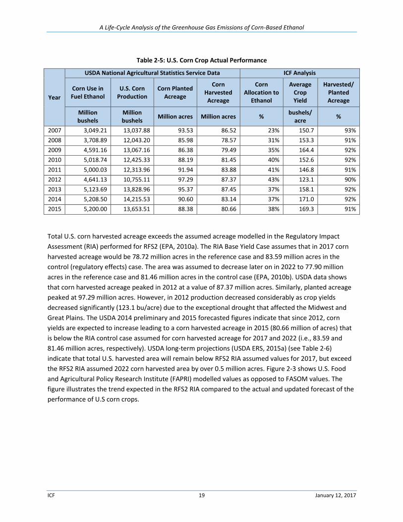
A Life-Cycle Analysis of the Greenhouse Gas Emissions of Corn-Based Ethanol
ICF 19 January 12, 2017
Table 2-5: U.S. Corn Crop Actual Performance
Year
USDA National Agricultural Statistics Service Data ICF Analysis
Corn Use in Fuel Ethanol
U.S. Corn Production
Corn Planted Acreage
Corn Harvested Acreage
Corn Allocation to
Ethanol
Average Crop Yield
Harvested/ Planted Acreage
Million bushels
Million bushels
Million acres Million acres % bushels/
acre %
2007 3,049.21 13,037.88 93.53 86.52 23% 150.7 93%
2008 3,708.89 12,043.20 85.98 78.57 31% 153.3 91%
2009 4,591.16 13,067.16 86.38 79.49 35% 164.4 92%
2010 5,018.74 12,425.33 88.19 81.45 40% 152.6 92%
2011 5,000.03 12,313.96 91.94 83.88 41% 146.8 91%
2012 4,641.13 10,755.11 97.29 87.37 43% 123.1 90%
2013 5,123.69 13,828.96 95.37 87.45 37% 158.1 92%
2014 5,208.50 14,215.53 90.60 83.14 37% 171.0 92%
2015 5,200.00 13,653.51 88.38 80.66 38% 169.3 91%
Total U.S. corn harvested acreage exceeds the assumed acreage modelled in the Regulatory Impact
Assessment (RIA) performed for RFS2 (EPA, 2010a). The RIA Base Yield Case assumes that in 2017 corn
harvested acreage would be 78.72 million acres in the reference case and 83.59 million acres in the
control (regulatory effects) case. The area was assumed to decrease later on in 2022 to 77.90 million
acres in the reference case and 81.46 million acres in the control case (EPA, 2010b). USDA data shows
that corn harvested acreage peaked in 2012 at a value of 87.37 million acres. Similarly, planted acreage
peaked at 97.29 million acres. However, in 2012 production decreased considerably as crop yields
decreased significantly (123.1 bu/acre) due to the exceptional drought that affected the Midwest and
Great Plains. The USDA 2014 preliminary and 2015 forecasted figures indicate that since 2012, corn
yields are expected to increase leading to a corn harvested acreage in 2015 (80.66 million of acres) that
is below the RIA control case assumed for corn harvested acreage for 2017 and 2022 (i.e., 83.59 and
81.46 million acres, respectively). USDA long-term projections (USDA ERS, 2015a) (see Table 2-6)
indicate that total U.S. harvested area will remain below RFS2 RIA assumed values for 2017, but exceed
the RFS2 RIA assumed 2022 corn harvested area by over 0.5 million acres. Figure 2-3 shows U.S. Food
and Agricultural Policy Research Institute (FAPRI) modelled values as opposed to FASOM values. The
figure illustrates the trend expected in the RFS2 RIA compared to the actual and updated forecast of the
performance of U.S corn crops.
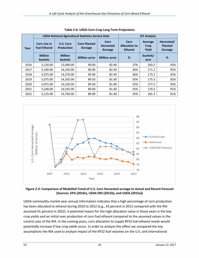
A Life-Cycle Analysis of the Greenhouse Gas Emissions of Corn-Based Ethanol
ICF 20 January 12, 2017
Table 2-6: USDA Corn Crop Long Term Projections
Year
USDA National Agricultural Statistics Service Data ICF Analysis
Corn Use in Fuel Ethanol
U.S. Corn Production
Corn Planted Acreage
Corn Harvested Acreage
Corn Allocation to
Ethanol
Average Crop Yield
Harvested/ Planted Acreage
Million bushels
Million bushels
Million acres Million acres % bushels/
acre %
2016 5,150.00 13,940.00 90.00 82.40 37% 169.2 92%
2017 5,100.00 14,105.00 90.00 82.40 36% 171.2 92%
2018 5,075.00 14,270.00 90.00 82.40 36% 173.2 92%
2019 5,075.00 14,355.00 89.50 81.90 35% 175.3 92%
2020 5,075.00 14,520.00 89.50 81.90 35% 177.3 92%
2021 5,100.00 14,595.00 89.00 81.40 35% 179.3 91%
2022 5,125.00 14,760.00 89.00 81.40 35% 181.3 91%
Figure 2-3: Comparison of Modelled Trend of U.S. Corn Harvested acreage to Actual and Recent Forecast (Sources: EPA (2010c), USDA ERS (2015b), and USDA (2015a))
USDA commodity market year annual information indicates that a high percentage of corn production
has been allocated to ethanol during 2010 to 2012 (e.g., 43 percent in 2012 compared with the RIA
assumed 41 percent in 2022). A potential reason for the high allocation value in those years is the low
crop yields and an initial over production of corn fuel ethanol compared to the assumed values in the
control case of the RIA. In the coming years, corn allocation to supply RFS2 fuel ethanol needs would
potentially increase if low crop yields occur. In order to analyze this effect we compared the key
assumptions the RIA used to analyze impact of the RFS2 fuel volumes on the U.S. and international
78
79
80
81
82
83
84
85
86
87
88
2007 2010 2013 2016 2019 2022
U.S
. Co
rn H
arve
sted
Acr
eage
(M
illio
n o
f A
cres
)
Year
Control Case
Reference
USDA MY Statistics
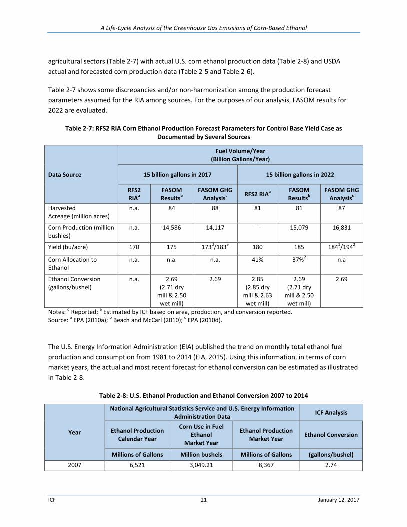
A Life-Cycle Analysis of the Greenhouse Gas Emissions of Corn-Based Ethanol
ICF 21 January 12, 2017
agricultural sectors (Table 2-7) with actual U.S. corn ethanol production data (Table 2-8) and USDA
actual and forecasted corn production data (Table 2-5 and Table 2-6).
Table 2-7 shows some discrepancies and/or non-harmonization among the production forecast
parameters assumed for the RIA among sources. For the purposes of our analysis, FASOM results for
2022 are evaluated.
Table 2-7: RFS2 RIA Corn Ethanol Production Forecast Parameters for Control Base Yield Case as Documented by Several Sources
Data Source
Fuel Volume/Year (Billion Gallons/Year)
15 billion gallons in 2017 15 billion gallons in 2022
RFS2 RIA
a FASOM Results
b
FASOM GHG Analysis
c
RFS2 RIAa
FASOM Results
b
FASOM GHG Analysis
c
Harvested Acreage (million acres)
n.a. 84 88 81 81 87
Corn Production (million bushles)
n.a. 14,586 14,117 --- 15,079 16,831
Yield (bu/acre) 170 175 173d/183
e 180 185 184
1/194
2
Corn Allocation to Ethanol
n.a. n.a. n.a. 41% 37%2 n.a
Ethanol Conversion (gallons/bushel)
n.a. 2.69 (2.71 dry
mill & 2.50 wet mill)
2.69 2.85 (2.85 dry
mill & 2.63 wet mill)
2.69 (2.71 dry
mill & 2.50 wet mill)
2.69
Notes: d Reported;
e Estimated by ICF based on area, production, and conversion reported.
Source: a EPA (2010a);
b Beach and McCarl (2010);
c EPA (2010d).
The U.S. Energy Information Administration (EIA) published the trend on monthly total ethanol fuel
production and consumption from 1981 to 2014 (EIA, 2015). Using this information, in terms of corn
market years, the actual and most recent forecast for ethanol conversion can be estimated as illustrated
in Table 2-8.
Table 2-8: U.S. Ethanol Production and Ethanol Conversion 2007 to 2014
Year
National Agricultural Statistics Service and U.S. Energy Information Administration Data
ICF Analysis
Ethanol Production Calendar Year
Corn Use in Fuel Ethanol
Market Year
Ethanol Production Market Year
Ethanol Conversion
Millions of Gallons Million bushels Millions of Gallons (gallons/bushel)
2007 6,521 3,049.21 8,367 2.74
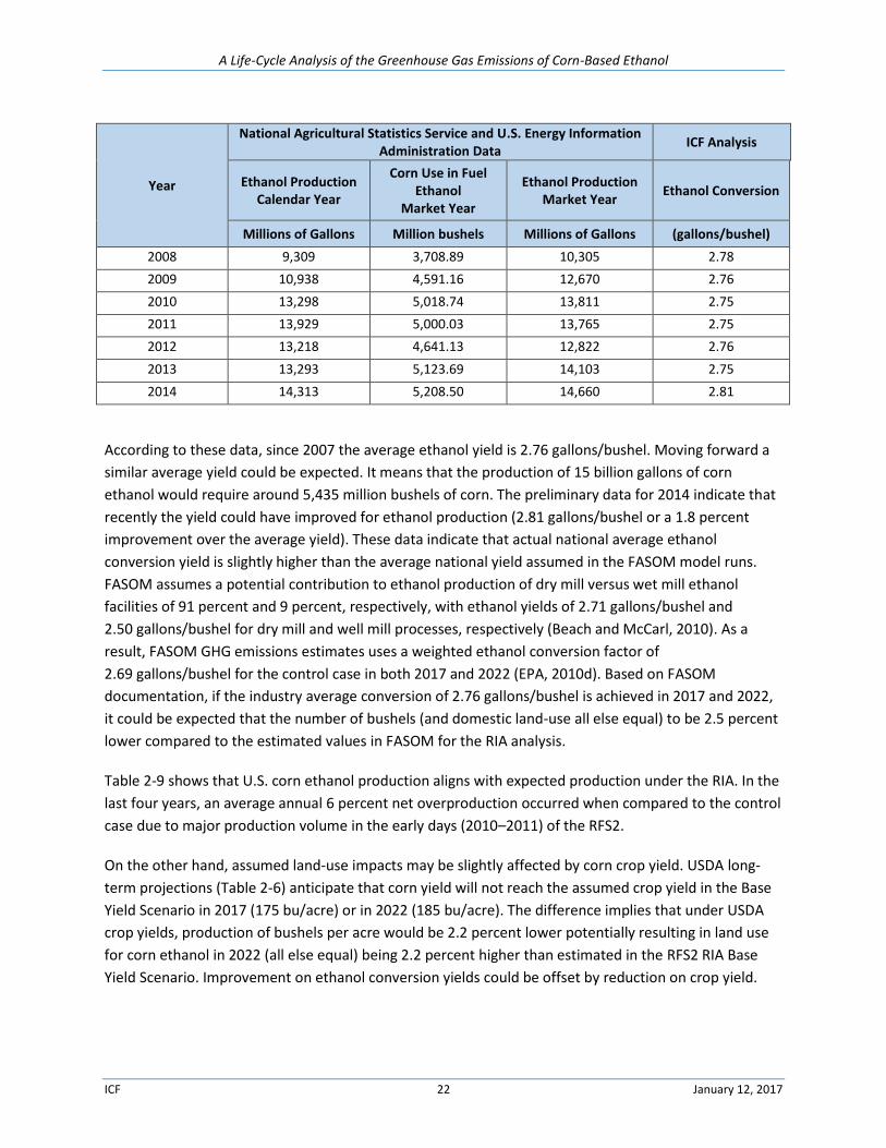
A Life-Cycle Analysis of the Greenhouse Gas Emissions of Corn-Based Ethanol
ICF 22 January 12, 2017
Year
National Agricultural Statistics Service and U.S. Energy Information Administration Data
ICF Analysis
Ethanol Production Calendar Year
Corn Use in Fuel Ethanol
Market Year
Ethanol Production Market Year
Ethanol Conversion
Millions of Gallons Million bushels Millions of Gallons (gallons/bushel)
2008 9,309 3,708.89 10,305 2.78
2009 10,938 4,591.16 12,670 2.76
2010 13,298 5,018.74 13,811 2.75
2011 13,929 5,000.03 13,765 2.75
2012 13,218 4,641.13 12,822 2.76
2013 13,293 5,123.69 14,103 2.75
2014 14,313 5,208.50 14,660 2.81
According to these data, since 2007 the average ethanol yield is 2.76 gallons/bushel. Moving forward a
similar average yield could be expected. It means that the production of 15 billion gallons of corn
ethanol would require around 5,435 million bushels of corn. The preliminary data for 2014 indicate that
recently the yield could have improved for ethanol production (2.81 gallons/bushel or a 1.8 percent
improvement over the average yield). These data indicate that actual national average ethanol
conversion yield is slightly higher than the average national yield assumed in the FASOM model runs.
FASOM assumes a potential contribution to ethanol production of dry mill versus wet mill ethanol
facilities of 91 percent and 9 percent, respectively, with ethanol yields of 2.71 gallons/bushel and
2.50 gallons/bushel for dry mill and well mill processes, respectively (Beach and McCarl, 2010). As a
result, FASOM GHG emissions estimates uses a weighted ethanol conversion factor of
2.69 gallons/bushel for the control case in both 2017 and 2022 (EPA, 2010d). Based on FASOM
documentation, if the industry average conversion of 2.76 gallons/bushel is achieved in 2017 and 2022,
it could be expected that the number of bushels (and domestic land-use all else equal) to be 2.5 percent
lower compared to the estimated values in FASOM for the RIA analysis.
Table 2-9 shows that U.S. corn ethanol production aligns with expected production under the RIA. In the
last four years, an average annual 6 percent net overproduction occurred when compared to the control
case due to major production volume in the early days (2010–2011) of the RFS2.
On the other hand, assumed land-use impacts may be slightly affected by corn crop yield. USDA long-
term projections (Table 2-6) anticipate that corn yield will not reach the assumed crop yield in the Base
Yield Scenario in 2017 (175 bu/acre) or in 2022 (185 bu/acre). The difference implies that under USDA
crop yields, production of bushels per acre would be 2.2 percent lower potentially resulting in land use
for corn ethanol in 2022 (all else equal) being 2.2 percent higher than estimated in the RFS2 RIA Base
Yield Scenario. Improvement on ethanol conversion yields could be offset by reduction on crop yield.
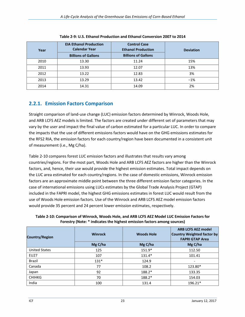
A Life-Cycle Analysis of the Greenhouse Gas Emissions of Corn-Based Ethanol
ICF 23 January 12, 2017
Table 2-9: U.S. Ethanol Production and Ethanol Conversion 2007 to 2014
Year
EIA Ethanol Production Calendar Year
Control Case
Ethanol Production Deviation
Billions of Gallons Billions of Gallons
2010 13.30 11.24 15%
2011 13.93 12.07 13%
2012 13.22 12.83 3%
2013 13.29 13.42 −1%
2014 14.31 14.09 2%
2.2.1. Emission Factors Comparison
Straight comparison of land-use change (LUC) emission factors determined by Winrock, Woods Hole,
and ARB LCFS AEZ models is limited. The factors are created under different set of parameters that may
vary by the user and impact the final value of carbon estimated for a particular LUC. In order to compare
the impacts that the use of different emissions factors would have on the GHG emissions estimates for
the RFS2 RIA, the emission factors for each country/region have been documented in a consistent unit
of measurement (i.e., Mg C/ha).
Table 2-10 compares forest LUC emission factors and illustrates that results vary among
countries/regions. For the most part, Woods Hole and ARB LCFS AEZ factors are higher than the Winrock
factors, and, hence, their use would provide the highest emission estimates. Total impact depends on
the LUC area estimated for each country/regions. In the case of domestic emissions, Winrock emission
factors are an approximate middle point between the three different emission factor categories. In the
case of international emissions using LUCs estimates by the Global Trade Analysis Project (GTAP)
included in the FAPRI model, the highest GHG emissions estimates in forest LUC would result from the
use of Woods Hole emission factors. Use of the Winrock and ARB LCFS AEZ model emission factors
would provide 35 percent and 24 percent lower emission estimates, respectively.
Table 2-10: Comparison of Winrock, Woods Hole, and ARB LCFS AEZ Model LUC Emission Factors for Forestry (Note: * indicates the highest emission factors among sources)
Country/Region Winrock Woods Hole
ARB LCFS AEZ model Country Weighted factor by
FAPRI GTAP Area
Mg C/ha Mg C/ha Mg C/ha
United States 125 151.9* 112.50
EU27 107 131.4* 101.41
Brazil 131* 124.9 -
Canada 77 108.2 123.80*
Japan 92 188.2* 133.35
CHIHKG 70 188.2* 154.03
India 100 131.4 196.21*
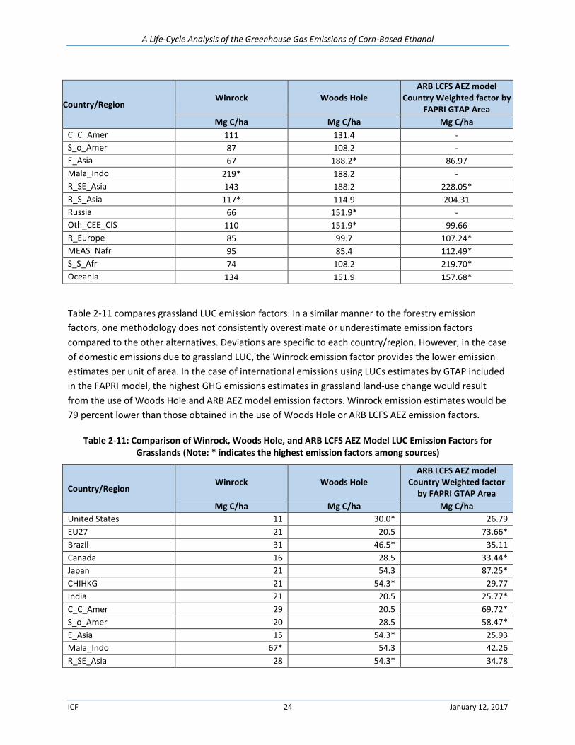
A Life-Cycle Analysis of the Greenhouse Gas Emissions of Corn-Based Ethanol
ICF 24 January 12, 2017
Country/Region Winrock Woods Hole
ARB LCFS AEZ model Country Weighted factor by
FAPRI GTAP Area
Mg C/ha Mg C/ha Mg C/ha
C_C_Amer 111 131.4 -
S_o_Amer 87 108.2 -
E_Asia 67 188.2* 86.97
Mala_Indo 219* 188.2 -
R_SE_Asia 143 188.2 228.05*
R_S_Asia 117* 114.9 204.31
Russia 66 151.9* -
Oth_CEE_CIS 110 151.9* 99.66
R_Europe 85 99.7 107.24*
MEAS_Nafr 95 85.4 112.49*
S_S_Afr 74 108.2 219.70*
Oceania 134 151.9 157.68*
Table 2-11 compares grassland LUC emission factors. In a similar manner to the forestry emission
factors, one methodology does not consistently overestimate or underestimate emission factors
compared to the other alternatives. Deviations are specific to each country/region. However, in the case
of domestic emissions due to grassland LUC, the Winrock emission factor provides the lower emission
estimates per unit of area. In the case of international emissions using LUCs estimates by GTAP included
in the FAPRI model, the highest GHG emissions estimates in grassland land-use change would result
from the use of Woods Hole and ARB AEZ model emission factors. Winrock emission estimates would be
79 percent lower than those obtained in the use of Woods Hole or ARB LCFS AEZ emission factors.
Table 2-11: Comparison of Winrock, Woods Hole, and ARB LCFS AEZ Model LUC Emission Factors for Grasslands (Note: * indicates the highest emission factors among sources)
Country/Region Winrock Woods Hole
ARB LCFS AEZ model Country Weighted factor
by FAPRI GTAP Area
Mg C/ha Mg C/ha Mg C/ha
United States 11 30.0* 26.79
EU27 21 20.5 73.66*
Brazil 31 46.5* 35.11
Canada 16 28.5 33.44*
Japan 21 54.3 87.25*
CHIHKG 21 54.3* 29.77
India 21 20.5 25.77*
C_C_Amer 29 20.5 69.72*
S_o_Amer 20 28.5 58.47*
E_Asia 15 54.3* 25.93
Mala_Indo 67* 54.3 42.26
R_SE_Asia 28 54.3* 34.78
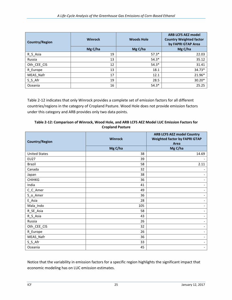
A Life-Cycle Analysis of the Greenhouse Gas Emissions of Corn-Based Ethanol
ICF 25 January 12, 2017
Country/Region Winrock Woods Hole
ARB LCFS AEZ model Country Weighted factor
by FAPRI GTAP Area
Mg C/ha Mg C/ha Mg C/ha
R_S_Asia 19 57.3* 22.03
Russia 13 54.3* 35.12
Oth_CEE_CIS 12 54.3* 31.41
R_Europe 13 18.1 34.73*
MEAS_Nafr 17 12.1 21.96*
S_S_Afr 19 28.5 30.20*
Oceania 16 54.3* 25.25
Table 2-12 indicates that only Winrock provides a complete set of emission factors for all different
countries/regions in the category of Cropland Pasture. Wood Hole does not provide emission factors
under this category and ARB provides only two data points.
Table 2-12: Comparison of Winrock, Wood Hole, and ARB LCFS AEZ Model LUC Emission Factors for Cropland Pasture
Country/Region Winrock
ARB LCFS AEZ model Country Weighted factor by FAPRI GTAP
Area
Mg C/ha Mg C/ha
United States 38 14.69
EU27 39 -
Brazil 58 2.11
Canada 32 -
Japan 38 -
CHIHKG 36 -
India 41 -
C_C_Amer 49 -
S_o_Amer 36 -
E_Asia 28 -
Mala_Indo 105 -
R_SE_Asia 58 -
R_S_Asia 43 -
Russia 26 -
Oth_CEE_CIS 32 -
R_Europe 26 -
MEAS_Nafr 36 -
S_S_Afr 33 -
Oceania 45 -
Notice that the variability in emission factors for a specific region highlights the significant impact that
economic modeling has on LUC emission estimates.
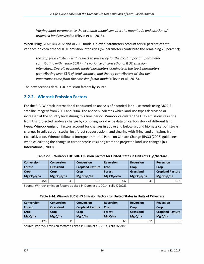
A Life-Cycle Analysis of the Greenhouse Gas Emissions of Corn-Based Ethanol
ICF 26 January 12, 2017
Varying input parameter to the economic model can alter the magnitude and location of
projected land conversion (Plevin et al., 2015).
When using GTAP-BIO-ADV and AEZ-EF models, eleven parameters account for 80 percent of total
variance on corn ethanol ILUC emission intensities (57 parameters contribute the remaining 20 percent);
the crop yield elasticity with respect to price is by far the most important parameter
contributing with nearly 50% in the variance of corn ethanol ILUC emission
intensities…Overall, economic model parameters dominate in the top 5 parameters
(contributing over 65% of total variance) and the top contributors of `3rd tier`
importance came from the emission factor model (Plevin et al., 2015).
The next sections detail LUC emission factors by source.
2.2.2. Winrock Emission Factors
For the RIA, Winrock International conducted an analysis of historical land-use trends using MODIS
satellite imagery from 2001 and 2004. The analysis indicates which land-use types decreased or
increased at the country level during this time period. Winrock calculated the GHG emissions resulting
from this projected land-use change by compiling world wide data on carbon stock of different land
types. Winrock emission factors account for changes in above and below-ground biomass carbon stocks,
changes in soils carbon stocks, lost forest sequestration, land clearing with firing, and emissions from
rice cultivation. Winrock followed Intergovernmental Panel on Climate Change (IPCC) (2006) guidelines
when calculating the change in carbon stocks resulting from the projected land-use changes (ICF
International, 2009).
Table 2-13: Winrock LUC GHG Emission Factors for United States in Units of CO2e/hectare
Conversion Conversion Conversion Reversion Reversion Reversion
Forest Grassland Cropland Pasture Crop Crop Crop
Crop Crop Crop Forest Grassland Cropland Pasture
Mg CO2e/ha Mg CO2e/ha Mg CO2e/ha Mg CO2e/ha Mg CO2e/ha Mg CO2e/ha
458 41 138 −237 −41 −138
Source: Winrock emission factors as cited in Dunn et al., 2014, cells J79:O83
Table 2-14: Winrock LUC GHG Emission Factors for United States in Units of C/hectare
Conversion Conversion Conversion Reversion Reversion Reversion
Forest Grassland Cropland Pasture Crop Crop Crop
Crop Crop Crop Forest Grassland Cropland Pasture
Mg C/ha Mg C/ha Mg C/ha Mg C/ha Mg C/ha Mg C/ha
125 11 38 −65 −11 −38
Source: Winrock emission factors as cited in Dunn et al., 2014, cells D79:I83
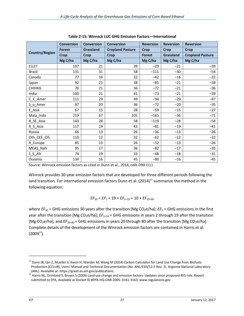
A Life-Cycle Analysis of the Greenhouse Gas Emissions of Corn-Based Ethanol
ICF 27 January 12, 2017
Table 2-15: Winrock LUC GHG Emission Factors—International
Country/Region
Conversion Conversion Conversion Reversion Reversion Reversion
Forest Grassland Cropland Pasture Crop Crop Crop
Crop Crop Crop Forest Grassland Cropland Pasture
Mg C/ha Mg C/ha Mg C/ha Mg C/ha Mg C/ha Mg C/ha
EU27 107 21 39 −29 −21 −39
Brazil 131 31 58 −111 −30 −54
Canada 77 16 32 −42 −16 −32
Japan 92 21 38 −85 −21 −38
CHIHKG 70 21 36 −72 −21 −36
India 100 21 41 −73 −21 −39
C_C_Amer 111 29 49 −94 −29 −47
S_o_Amer 87 20 36 −72 −20 −35
E_Asia 67 15 28 −59 −15 −27
Mala_Indo 219 67 105 −165 −36 −71
R_SE_Asia 143 28 58 −119 −28 −54
R_S_Asia 117 19 43 −81 −19 −41
Russia 66 13 26 −36 −13 −26
Oth_CEE_CIS 110 12 32 −62 −12 −32
R_Europe 85 13 26 −52 −13 −26
MEAS_Nafr 95 17 36 −82 −17 −35
S_S_Afr 74 19 33 −48 −18 −31
Oceania 134 16 45 −80 −16 -45
Source: Winrock emission factors as cited in Dunn et al., 2014, cells D90:I111
Winrock provides 30-year emission factors that are developed for three different periods following the
land transition. For international emission factors Dunn et al. (2014)11 summarize the method in the
following equation:
EF30 = EF1 + 19 × EF2–19 + 10 × EF20–80
where EF30 = GHG emissions 30 years after the transition [Mg CO2e/ha]; EF1 = GHG emissions in the first
year after the transition [Mg CO2e/ha]; EF2–19 = GHG emissions in years 2 through 19 after the transition
[Mg CO2e/ha]; and EF20–80 = GHG emissions in years 20 through 80 after the transition [Mg CO2e/ha].
Complete details of the development of the Winrock emission factors are contained in Harris et al.
(200912).
11 Dunn JB, Qin Z, Mueller S, Kwon H, Wander M, Wang M (2014) Carbon Calculator for Land Use Change from Biofuels Production (CCLUB), Users' Manual and Technical Documentation (No. ANL/ESD/12-5 Rev. 2). Argonne National Laboratory (ANL). Available at: https://greet.es.anl.gov/publications.
12 Harris NL, Grimland S, Brown S (2009) Land use change and emission factors: Updates since proposed RFS rule. Report submitted to EPA, Available at Docket ID #EPA-HQ-OAR-2005- 0161-3163, www.regulations.gov
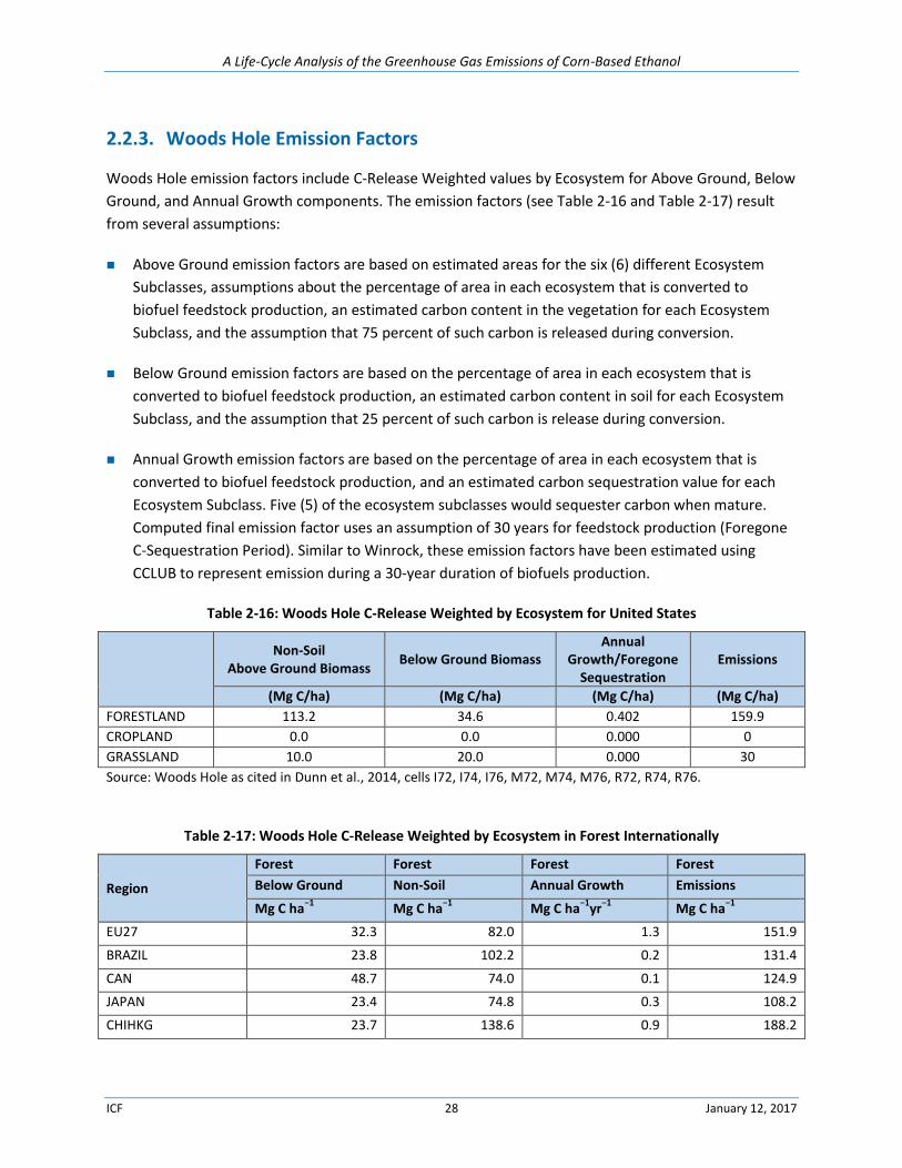
A Life-Cycle Analysis of the Greenhouse Gas Emissions of Corn-Based Ethanol
ICF 28 January 12, 2017
2.2.3. Woods Hole Emission Factors
Woods Hole emission factors include C-Release Weighted values by Ecosystem for Above Ground, Below
Ground, and Annual Growth components. The emission factors (see Table 2-16 and Table 2-17) result
from several assumptions:
Above Ground emission factors are based on estimated areas for the six (6) different Ecosystem
Subclasses, assumptions about the percentage of area in each ecosystem that is converted to
biofuel feedstock production, an estimated carbon content in the vegetation for each Ecosystem
Subclass, and the assumption that 75 percent of such carbon is released during conversion.
Below Ground emission factors are based on the percentage of area in each ecosystem that is
converted to biofuel feedstock production, an estimated carbon content in soil for each Ecosystem
Subclass, and the assumption that 25 percent of such carbon is release during conversion.
Annual Growth emission factors are based on the percentage of area in each ecosystem that is
converted to biofuel feedstock production, and an estimated carbon sequestration value for each
Ecosystem Subclass. Five (5) of the ecosystem subclasses would sequester carbon when mature.
Computed final emission factor uses an assumption of 30 years for feedstock production (Foregone
C-Sequestration Period). Similar to Winrock, these emission factors have been estimated using
CCLUB to represent emission during a 30-year duration of biofuels production.
Table 2-16: Woods Hole C-Release Weighted by Ecosystem for United States
Non-Soil
Above Ground Biomass Below Ground Biomass
Annual Growth/Foregone
Sequestration Emissions
(Mg C/ha) (Mg C/ha) (Mg C/ha) (Mg C/ha)
FORESTLAND 113.2 34.6 0.402 159.9
CROPLAND 0.0 0.0 0.000 0
GRASSLAND 10.0 20.0 0.000 30
Source: Woods Hole as cited in Dunn et al., 2014, cells I72, I74, I76, M72, M74, M76, R72, R74, R76.
Table 2-17: Woods Hole C-Release Weighted by Ecosystem in Forest Internationally
Region
Forest Forest Forest Forest
Below Ground Non-Soil Annual Growth Emissions
Mg C ha−1
Mg C ha−1
Mg C ha−1
yr−1
Mg C ha−1
EU27 32.3 82.0 1.3 151.9
BRAZIL 23.8 102.2 0.2 131.4
CAN 48.7 74.0 0.1 124.9
JAPAN 23.4 74.8 0.3 108.2
CHIHKG 23.7 138.6 0.9 188.2
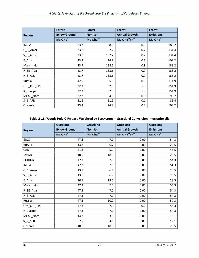
A Life-Cycle Analysis of the Greenhouse Gas Emissions of Corn-Based Ethanol
ICF 29 January 12, 2017
Region
Forest Forest Forest Forest
Below Ground Non-Soil Annual Growth Emissions
Mg C ha−1
Mg C ha−1
Mg C ha−1
yr−1
Mg C ha−1
INDIA 23.7 138.6 0.9 188.2
C_C_Amer 23.8 102.2 0.2 131.4
S_o_Amer 23.8 102.2 0.2 131.4
E_Asia 23.4 74.8 0.3 108.2
Mala_Indo 23.7 138.6 0.9 188.2
R_SE_Asia 23.7 138.6 0.9 188.2
R_S_Asia 23.7 138.6 0.9 188.2
Russia 42.0 65.0 0.3 114.9
Oth_CEE_CIS 32.3 82.0 1.3 151.9
R_Europe 32.3 82.0 1.3 151.9
MEAS_NAfr 22.2 54.9 0.8 99.7
S_S_AFR 31.6 51.9 0.1 85.4
Oceania 23.4 74.8 0.3 108.2
Table 2-18: Woods Hole C-Release Weighted by Ecosystem in Grassland Conversion Internationally
Region
Grassland Grassland Grassland Grassland
Below Ground Non-Soil Annual Growth Emissions
Mg C ha−1
Mg C ha−1
Mg C ha−1
yr−1
Mg C ha−1
EU27 47.3 7.0 0.00 54.3
BRAZIL 13.8 6.7 0.00 20.5
CAN 41.4 5.1 0.00 46.5
JAPAN 10.5 18.0 0.00 28.5
CHIHKG 47.3 7.0 0.00 54.3
INDIA 47.3 7.0 0.00 54.3
C_C_Amer 13.8 6.7 0.00 20.5
S_o_Amer 13.8 6.7 0.00 20.5
E_Asia 10.5 18.0 0.00 28.5
Mala_Indo 47.3 7.0 0.00 54.3
R_SE_Asia 47.3 7.0 0.00 54.3
R_S_Asia 47.3 7.0 0.00 54.3
Russia 47.3 10.0 0.00 57.3
Oth_CEE_CIS 47.3 7.0 0.0 54.3
R_Europe 47.3 7.0 0.00 54.3
MEAS_NAfr 14.3 3.8 0.00 18.1
S_S_AFR 7.5 4.6 0.00 12.1
Oceania 10.5 18.0 0.00 28.5
A Life-Cycle Analysis of the Greenhouse Gas Emissions of Corn-Based Ethanol
ICF 30 January 12, 2017
Source: Woods Hole as cited in Dunn et al., 2014, cells B73:T93. Assumption: Input 6: Feedstock Production Years (Foregone C-Sequestration Period) = 30 years Production Years (Foregone C-Sequestration Period) = 30 years
2.2.4. Air Resources Board Low-Carbon Fuel Standard Agro-Ecological Zone Model
The Air Resources Board (ARB) Low-Carbon Fuel Standard (LCFS) Agro-Ecological Zone (AEZ) model
provides U.S. and international LUC emission factors for the conversion of forestry, pasture, cropland
pasture, and annuals. The model emission factors are disaggregated by world region and agro-ecological
zones (AEZs). The model is consistent with the 19 regions and 18 zones reported by GTAP-BIO (GTAP
biofuels) model. As a result, the model combines matrices of carbon fluxes (Mg CO2 ha−1yr−1) with
matrices of changes in land use (ha) according to land-use category as projected by the GTAP-BIO
model. The model also includes indexed carbon stock estimates (MgC ha−1) for biomass and soil carbon
by the GTAP AEZ and region. The model uses assumptions about carbon loss from soils, biomass, mode
of conversion, quantity and species of carbonaceous, and other GHG emissions resulting from
conversion and carbon remaining in harvested wood products and char, and foregone sequestration
(CARB, 2015). The full analytic time horizon used in AEZ-EF model is 30 years (Plevin et al, 201513).
Table 2-19 shows the emission factors for Forest to Annuals, Pasture to Annuals, and CroplandPasture to
Annuals that can be compared to the emission factors developed by Winrock or Woods Hole. In order to
do a comparison, the emission factors that are provided by region and AEZ should be converted into
equivalent emission factors by country/region. The country/region equivalent emission factors are
weighted based on LUC area in each AEZ estimated by GTAP. Table 2-20 shows the equivalent emission
factors.
13 Plevin et al.,2015. Carbon Accounting and Economic Model Uncertainty of Emissions from Biofuels-Induced Land Use Change. Environmental Science & Technology, 49(5). March 3, 2015. http://escholarship.org/uc/item/9wz1r8gf
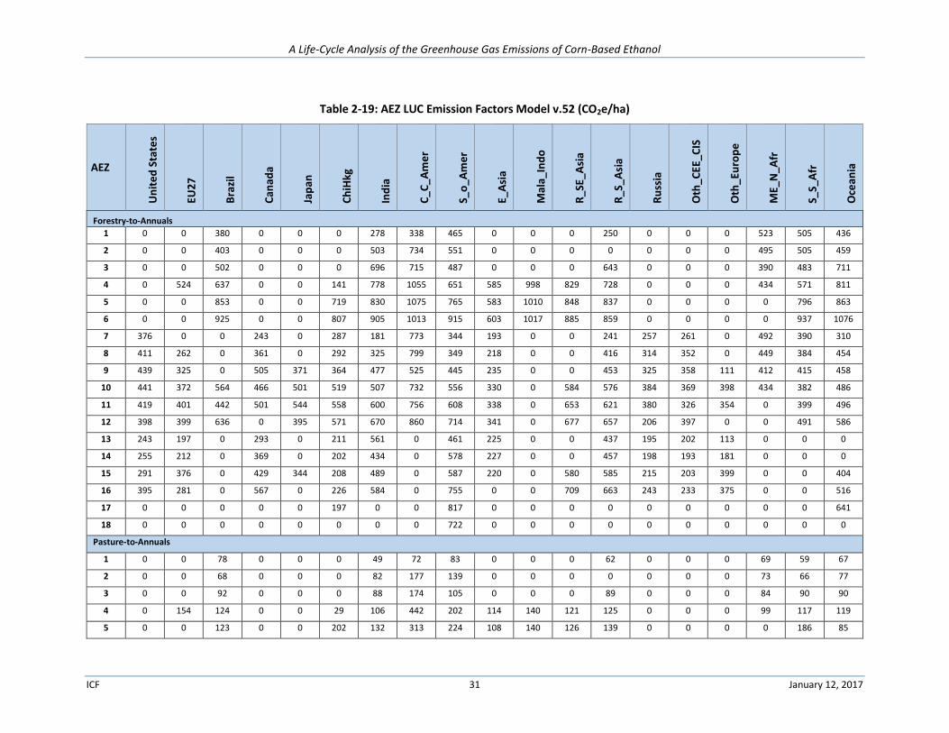
A Life-Cycle Analysis of the Greenhouse Gas Emissions of Corn-Based Ethanol
ICF 31 January 12, 2017
Table 2-19: AEZ LUC Emission Factors Model v.52 (CO2e/ha)
AEZ
Un
ite
d S
tate
s
EU2
7
Bra
zil
Can
ada
Jap
an
Ch
iHkg
Ind
ia
C_C
_A
me
r
S_o
_A
me
r
E_A
sia
Mal
a_In
do
R_S
E_A
sia
R_S
_A
sia
Ru
ssia
Oth
_CEE
_CIS
Oth
_Eu
rop
e
ME_
N_A
fr
S_S_
Afr
Oce
ania
Forestry-to-Annuals
1 0 0 380 0 0 0 278 338 465 0 0 0 250 0 0 0 523 505 436
2 0 0 403 0 0 0 503 734 551 0 0 0 0 0 0 0 495 505 459
3 0 0 502 0 0 0 696 715 487 0 0 0 643 0 0 0 390 483 711
4 0 524 637 0 0 141 778 1055 651 585 998 829 728 0 0 0 434 571 811
5 0 0 853 0 0 719 830 1075 765 583 1010 848 837 0 0 0 0 796 863
6 0 0 925 0 0 807 905 1013 915 603 1017 885 859 0 0 0 0 937 1076
7 376 0 0 243 0 287 181 773 344 193 0 0 241 257 261 0 492 390 310
8 411 262 0 361 0 292 325 799 349 218 0 0 416 314 352 0 449 384 454
9 439 325 0 505 371 364 477 525 445 235 0 0 453 325 358 111 412 415 458
10 441 372 564 466 501 519 507 732 556 330 0 584 576 384 369 398 434 382 486
11 419 401 442 501 544 558 600 756 608 338 0 653 621 380 326 354 0 399 496
12 398 399 636 0 395 571 670 860 714 341 0 677 657 206 397 0 0 491 586
13 243 197 0 293 0 211 561 0 461 225 0 0 437 195 202 113 0 0 0
14 255 212 0 369 0 202 434 0 578 227 0 0 457 198 193 181 0 0 0
15 291 376 0 429 344 208 489 0 587 220 0 580 585 215 203 399 0 0 404
16 395 281 0 567 0 226 584 0 755 0 0 709 663 243 233 375 0 0 516
17 0 0 0 0 0 197 0 0 817 0 0 0 0 0 0 0 0 0 641
18 0 0 0 0 0 0 0 0 722 0 0 0 0 0 0 0 0 0 0
Pasture-to-Annuals
1 0 0 78 0 0 0 49 72 83 0 0 0 62 0 0 0 69 59 67
2 0 0 68 0 0 0 82 177 139 0 0 0 0 0 0 0 73 66 77
3 0 0 92 0 0 0 88 174 105 0 0 0 89 0 0 0 84 90 90
4 0 154 124 0 0 29 106 442 202 114 140 121 125 0 0 0 99 117 119
5 0 0 123 0 0 202 132 313 224 108 140 126 139 0 0 0 0 186 85
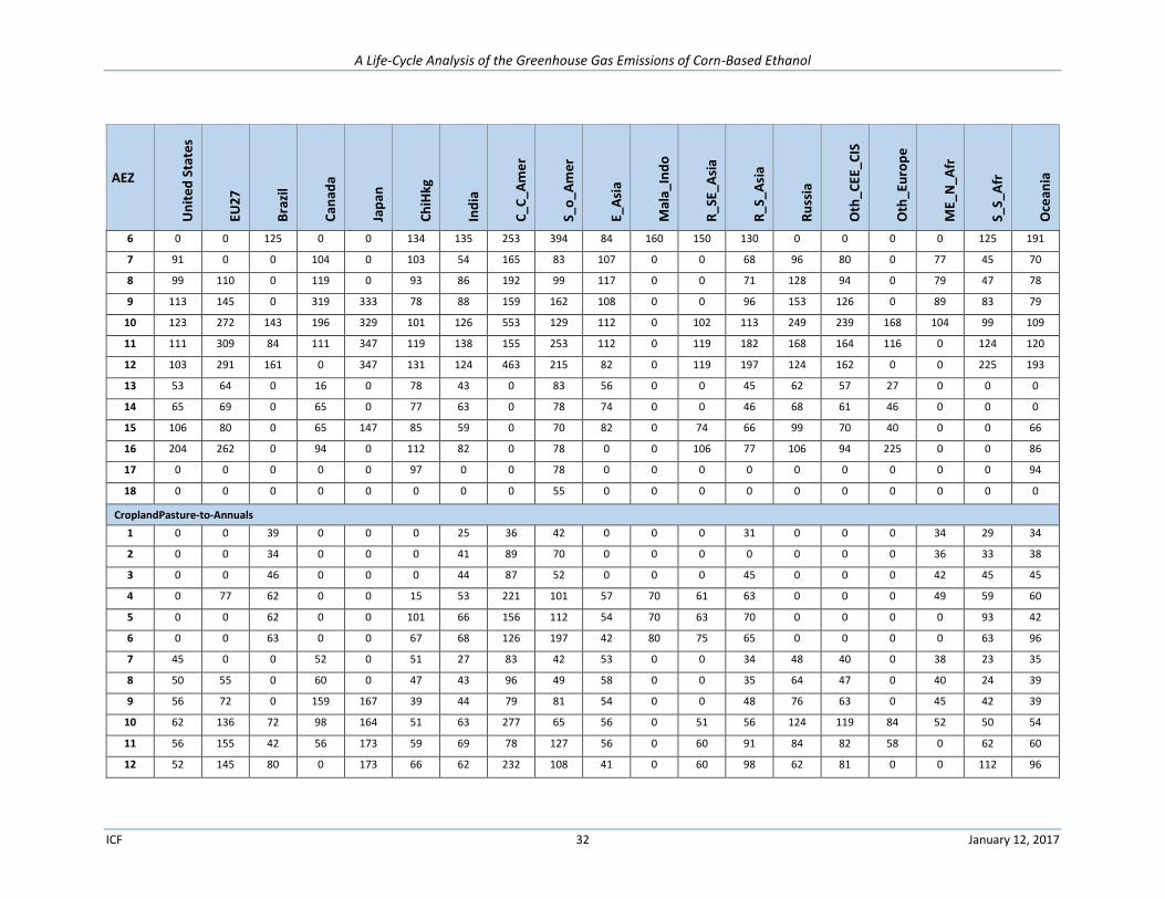
A Life-Cycle Analysis of the Greenhouse Gas Emissions of Corn-Based Ethanol
ICF 32 January 12, 2017
AEZ U
nit
ed
Sta
tes
EU2
7
Bra
zil
Can
ada
Jap
an
Ch
iHkg
Ind
ia
C_C
_A
me
r
S_o
_A
me
r
E_A
sia
Mal
a_In
do
R_S
E_A
sia
R_S
_A
sia
Ru
ssia
Oth
_CEE
_CIS
Oth
_Eu
rop
e
ME_
N_A
fr
S_S_
Afr
Oce
ania
6 0 0 125 0 0 134 135 253 394 84 160 150 130 0 0 0 0 125 191
7 91 0 0 104 0 103 54 165 83 107 0 0 68 96 80 0 77 45 70
8 99 110 0 119 0 93 86 192 99 117 0 0 71 128 94 0 79 47 78
9 113 145 0 319 333 78 88 159 162 108 0 0 96 153 126 0 89 83 79
10 123 272 143 196 329 101 126 553 129 112 0 102 113 249 239 168 104 99 109
11 111 309 84 111 347 119 138 155 253 112 0 119 182 168 164 116 0 124 120
12 103 291 161 0 347 131 124 463 215 82 0 119 197 124 162 0 0 225 193
13 53 64 0 16 0 78 43 0 83 56 0 0 45 62 57 27 0 0 0
14 65 69 0 65 0 77 63 0 78 74 0 0 46 68 61 46 0 0 0
15 106 80 0 65 147 85 59 0 70 82 0 74 66 99 70 40 0 0 66
16 204 262 0 94 0 112 82 0 78 0 0 106 77 106 94 225 0 0 86
17 0 0 0 0 0 97 0 0 78 0 0 0 0 0 0 0 0 0 94
18 0 0 0 0 0 0 0 0 55 0 0 0 0 0 0 0 0 0 0
CroplandPasture-to-Annuals
1 0 0 39 0 0 0 25 36 42 0 0 0 31 0 0 0 34 29 34
2 0 0 34 0 0 0 41 89 70 0 0 0 0 0 0 0 36 33 38
3 0 0 46 0 0 0 44 87 52 0 0 0 45 0 0 0 42 45 45
4 0 77 62 0 0 15 53 221 101 57 70 61 63 0 0 0 49 59 60
5 0 0 62 0 0 101 66 156 112 54 70 63 70 0 0 0 0 93 42
6 0 0 63 0 0 67 68 126 197 42 80 75 65 0 0 0 0 63 96
7 45 0 0 52 0 51 27 83 42 53 0 0 34 48 40 0 38 23 35
8 50 55 0 60 0 47 43 96 49 58 0 0 35 64 47 0 40 24 39
9 56 72 0 159 167 39 44 79 81 54 0 0 48 76 63 0 45 42 39
10 62 136 72 98 164 51 63 277 65 56 0 51 56 124 119 84 52 50 54
11 56 155 42 56 173 59 69 78 127 56 0 60 91 84 82 58 0 62 60
12 52 145 80 0 173 66 62 232 108 41 0 60 98 62 81 0 0 112 96
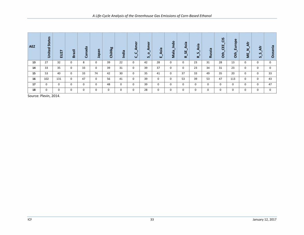
A Life-Cycle Analysis of the Greenhouse Gas Emissions of Corn-Based Ethanol
ICF 33 January 12, 2017
AEZ U
nit
ed
Sta
tes
EU2
7
Bra
zil
Can
ada
Jap
an
Ch
iHkg
Ind
ia
C_C
_A
me
r
S_o
_A
me
r
E_A
sia
Mal
a_In
do
R_S
E_A
sia
R_S
_A
sia
Ru
ssia
Oth
_CEE
_CIS
Oth
_Eu
rop
e
ME_
N_A
fr
S_S_
Afr
Oce
ania
13 27 32 0 8 0 39 22 0 42 28 0 0 23 31 28 13 0 0 0
14 33 35 0 33 0 39 31 0 39 37 0 0 23 34 31 23 0 0 0
15 53 40 0 33 74 42 30 0 35 41 0 37 33 49 35 20 0 0 33
16 102 131 0 47 0 56 41 0 39 0 0 53 39 53 47 113 0 0 43
17 0 0 0 0 0 48 0 0 39 0 0 0 0 0 0 0 0 0 47
18 0 0 0 0 0 0 0 0 28 0 0 0 0 0 0 0 0 0 0
Source: Plevin, 2014.
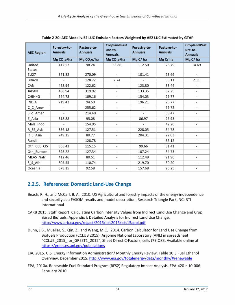
A Life-Cycle Analysis of the Greenhouse Gas Emissions of Corn-Based Ethanol
ICF 34 January 12, 2017
Table 2-20: AEZ Model v.52 LUC Emission Factors Weighted by AEZ LUC Estimated by GTAP
AEZ Region
Forestry-to-Annuals
Pasture-to-Annuals
CroplandPasture-to-Annuals
Forestry-to-Annuals
Pasture-to-Annuals
CroplandPasture-to-Annuals
Mg CO2e/ha Mg CO2e/ha Mg CO2e/ha Mg C/ ha Mg C/ ha Mg C/ ha
United States
412.52 98.24 53.86 112.50 26.79 14.69
EU27 371.82 270.09 - 101.41 73.66 -
BRAZIL - 128.72 7.74 - 35.11 2.11
CAN 453.94 122.62 - 123.80 33.44 -
JAPAN 488.94 319.92 - 133.35 87.25 -
CHIHKG 564.78 109.16 - 154.03 29.77 -
INDIA 719.42 94.50 - 196.21 25.77 -
C_C_Amer - 255.62 - - 69.72 -
S_o_Amer - 214.40 - - 58.47 -
E_Asia 318.88 95.08 - 86.97 25.93 -
Mala_Indo - 154.95 - - 42.26 -
R_SE_Asia 836.18 127.51 - 228.05 34.78 -
R_S_Asia 749.15 80.77 - 204.31 22.03 -
Russia - 128.78 - - 35.12 -
Oth_CEE_CIS 365.43 115.15 - 99.66 31.41 -
Oth_Europe 393.22 127.34 - 107.24 34.73 -
MEAS_Nafr 412.46 80.51 - 112.49 21.96 -
S_S_Afr 805.55 110.74 - 219.70 30.20 -
Oceania 578.15 92.58 - 157.68 25.25 -
2.2.5. References: Domestic Land-Use Change
Beach, R. H., and McCarl, B. A., 2010. US Agricultural and forestry impacts of the energy independence and security act: FASOM results and model description. Research Triangle Park, NC: RTI International.
CARB 2015. Staff Report: Calculating Carbon Intensity Values from Indirect Land Use Change and Crop Based Biofuels. Appendix I: Detailed Analysis for Indirect Land Use Change. http://www.arb.ca.gov/regact/2015/lcfs2015/lcfs15appi.pdf
Dunn, J.B., Mueller, S., Qin, Z., and Wang, M.Q., 2014. Carbon Calculator for Land Use Change from Biofuels Production (CCLUB 2015). Argonne National Laboratory (ANL) in spreadsheet “CCLUB_2015_for_GREET1_2015”, Sheet Direct C-Factors, cells J79:O83. Available online at https://greet.es.anl.gov/publications
EIA, 2015. U.S. Energy Information Administration/ Monthly Energy Review. Table 10.3 Fuel Ethanol Overview. December 2015. http://www.eia.gov/totalenergy/data/monthly/#renewable
EPA, 2010a. Renewable Fuel Standard Program (RFS2) Regulatory Impact Analysis. EPA-420-r-10-006. February 2010.
A Life-Cycle Analysis of the Greenhouse Gas Emissions of Corn-Based Ethanol
ICF 35 January 12, 2017
EPA, 2010b. Forestry and Agricultural Sector Optimization Model (FASOM) High Yield Sensitivity Comparison for Renewable Fuel Standard (RFS2). File:EPA-HQ-OAR-2005-0161-3180. http://www.regulations.gov/#!documentDetail;D=EPA-HQ-OAR-2005-0161-3180. Posted Mar 26, 2010.
EPA., 2010c. Life Cycle Analysis Results found in spreadsheet “Memorandum_to_Docket_SUBJECT_Fapri-Card_Lifecycle_GHG_(Greenhouse_Gases)_Analysis_Results,” Docket ID: EPA-HQ-OAR-2005-0161-3153. http://www.regulations.gov/#!documentDetail;D=EPA-HQ-OAR-2005-0161-3153
EPA, 2010d. Life Cycle Analysis Results found in spreadsheet “Forest_Agricultural_Sector_Optimization_Model_(FASOM)_Results_for_Lifecycle_Greenhouse_Gas_(GHG)” Docket ID: EPA-HQ-OAR-2005-0161-0948. Available online at: http://www.regulations.gov/#!documentDetail;D=EPA-HQ-OAR-2005-0161-0948
ICF International, 2009. Emissions from Land Use Change due to Increased Biofuel Production. Satellite Imagery and Emissions Factor Analysis. Peer Review Report.
Plevin, R. J., Beckman, J., Golub, A. A., Witcover, J., and O’Hare, M., 2015. Carbon Accounting and Economic Model Uncertainty of Emissions from Biofuels-Induced Land Use Change. Environmental Science & Technology, 49(5), 2656–2664.
Plevin, R.J., 2014. Agro-Ecological Zone Emissions Factor (AEZ-EF) Model in spreadsheet “aez-ef_model_v52.xls”, EF Sheet. Available online at www.arb.ca.gov/fuels/lcfs/lcfs_meetings/aez-ef_model_v52.xlsm
USDA ERS, 2015a. USDA Agricultural Projections, U.S. Department of Agriculture, Economic Research Service. http://www.ers.usda.gov/media/1776016/oce151d.pdf.
USDA ERS, 2015b. Feed Grains Database. U.S. Department of Agriculture, Economic Research Service. http://www.ers.usda.gov/data-products/feed-grains-database/documentation.aspx
USDA NASS, 1999. Understanding USDA Crop Forecasts. U.S. Departmnet of Agriculture, National Agricultural Statistics Service, and World Agricultural Outlook Board, Office of the Chief Economist http://www.nass.usda.gov/Education_and_Outreach/Understanding_Statistics/pub1554.pdf
2.3. Domestic Rice Methane
A review of the current literature shows that U.S. rice production and corresponding methane emissions
have remained relatively constant between 1990 through 2013. Harvested acres of rice have fluctuated
between ≈2.5 and 3.6 million acres, and emissions have fluctuated between 7.7 and 11.1 million metric
tons CO2 equivalent (MMT CO2e) (USDA ERS, 2015; EPA, 2015). The RFS2 RIA FASOM has higher
projections for future harvested rice acres than the current USDA Projections (USDA OCE, 2016). For
example, both the Control Case and the Reference Case have higher predicted harvested acres of rice in
2012 (3.8 million acres for the Reference Case and 3.35 million acres for the Control Case) than were
actually harvested in eight of the last nine years with 2010 as the only exception (USDA 2015).
Use of the RFS2 RIA emission factors for rice would under-estimate methane production from rice
cultivation in most regions between 1990 and 2013 when compared to effective emission factors from
A Life-Cycle Analysis of the Greenhouse Gas Emissions of Corn-Based Ethanol
ICF 36 January 12, 2017
the EPA Inventory (EPA, 2015). For example, the RFS2 RIA emission factor for the south central region
(where approximately70 percent of all rice production occurs) is 2,249.20 kg CO2e/acre compared to the
effective Inventory emission factor which ranges from approximately 2,800 to 3,100 kg CO2e/acre
between 1990–2013. The total projected 2012 rice methane emissions from the RFS2 RIA are nearly
double those of the EPA inventory despite the lower emission factors in the RFS2 RIA. The RFS2 RIA
estimated 2012 emissions are 17.8 MMTons CO2e for the Control Case and 18.41 MMT CO2e for the
Reference Case compared to 9.29 MMT CO2e from the EPA inventory and 8.78 MMT CO2e from the
Food and Agriculture Organization of the United Nations (FAO). The RFS2 RIA values seem inexplicably
high given the RFS2 RIA estimated acreage and the RFS2 RIA emission factors used. As the RFS2 RIA did
not provide all of the necessary underlying data, we could not reproduce the RFS2 RIA total emissions to
compare values to recent data.
2.3.1. Background on Methane from Rice Production
Methane is the primary greenhouse gas related to rice production (Gathorne-Hardy, 2013). All rice is the
United States is grown under continuously flooded, shallow water conditions where drainage does not
occur except by accident (EPA, 2015). Under flooded conditions, soils become anaerobic (lacking
oxygen) resulting in the production of methane (CH4) when soil organic matter is decomposed by
anaerobic methanogenic bacteria. A minor percentage of the methane produced (10–40 percent) is
released from the soil to the atmosphere either by diffusive transport through the rice plants, soil
diffusion or bubbling through floodwaters (EPA, 2015).
The amount of methane produced by rice cultivation is influenced by multiple factors (EPA, 2015;
Garthorne-Hardy, 2013; Hussain et al., 2015), including:
Water management practices (e.g., deepwater (greater than one meter) production, dryland
production, mid-season drainage, intermittent drainage)
Fertilizer practices (e.g., use of urea, ammonium nitrate, ammonium sulfate, organic fertilizers)
Residue management (e.g., straw removal, straw burning)
Soil temperature
Soil type
Rice cultivar
Cultivation practices (e.g., tillage, seeding and weeding practices)
2.3.2. Number of crops per season (e.g., primary and ratoon crop) U.S. Rice Production Area
Rice is currently produced in seven states: Arkansas, California, Louisiana, Mississippi, Missouri, and
Texas, and rice was produced in Oklahoma through 2007 (EPA, 2015; USDA ERS, 2015a). Figure 2-4
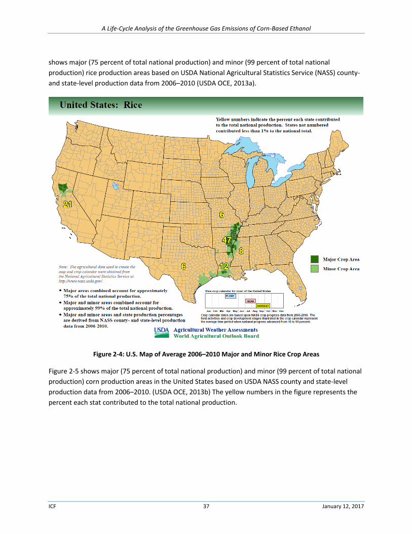
A Life-Cycle Analysis of the Greenhouse Gas Emissions of Corn-Based Ethanol
ICF 37 January 12, 2017
shows major (75 percent of total national production) and minor (99 percent of total national
production) rice production areas based on USDA National Agricultural Statistics Service (NASS) county-
and state-level production data from 2006–2010 (USDA OCE, 2013a).
Figure 2-4: U.S. Map of Average 2006–2010 Major and Minor Rice Crop Areas
Figure 2-5 shows major (75 percent of total national production) and minor (99 percent of total national
production) corn production areas in the United States based on USDA NASS county and state-level
production data from 2006–2010. (USDA OCE, 2013b) The yellow numbers in the figure represents the
percent each stat contributed to the total national production.
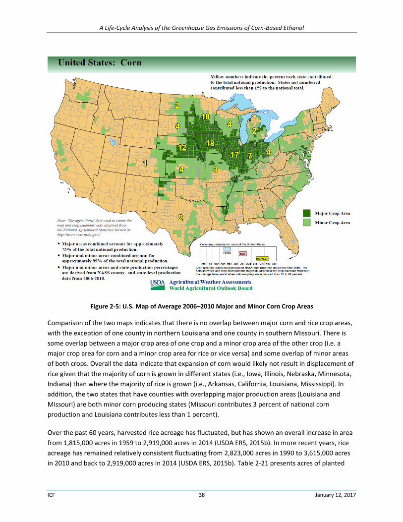
A Life-Cycle Analysis of the Greenhouse Gas Emissions of Corn-Based Ethanol
ICF 38 January 12, 2017
Figure 2-5: U.S. Map of Average 2006–2010 Major and Minor Corn Crop Areas
Comparison of the two maps indicates that there is no overlap between major corn and rice crop areas,
with the exception of one county in northern Louisiana and one county in southern Missouri. There is
some overlap between a major crop area of one crop and a minor crop area of the other crop (i.e. a
major crop area for corn and a minor crop area for rice or vice versa) and some overlap of minor areas
of both crops. Overall the data indicate that expansion of corn would likely not result in displacement of
rice given that the majority of corn is grown in different states (i.e., Iowa, Illinois, Nebraska, Minnesota,
Indiana) than where the majority of rice is grown (i.e., Arkansas, California, Louisiana, Mississippi). In
addition, the two states that have counties with overlapping major production areas (Louisiana and
Missouri) are both minor corn producing states (Missouri contributes 3 percent of national corn
production and Louisiana contributes less than 1 percent).
Over the past 60 years, harvested rice acreage has fluctuated, but has shown an overall increase in area
from 1,815,000 acres in 1959 to 2,919,000 acres in 2014 (USDA ERS, 2015b). In more recent years, rice
acreage has remained relatively consistent fluctuating from 2,823,000 acres in 1990 to 3,615,000 acres
in 2010 and back to 2,919,000 acres in 2014 (USDA ERS, 2015b). Table 2-21 presents acres of planted
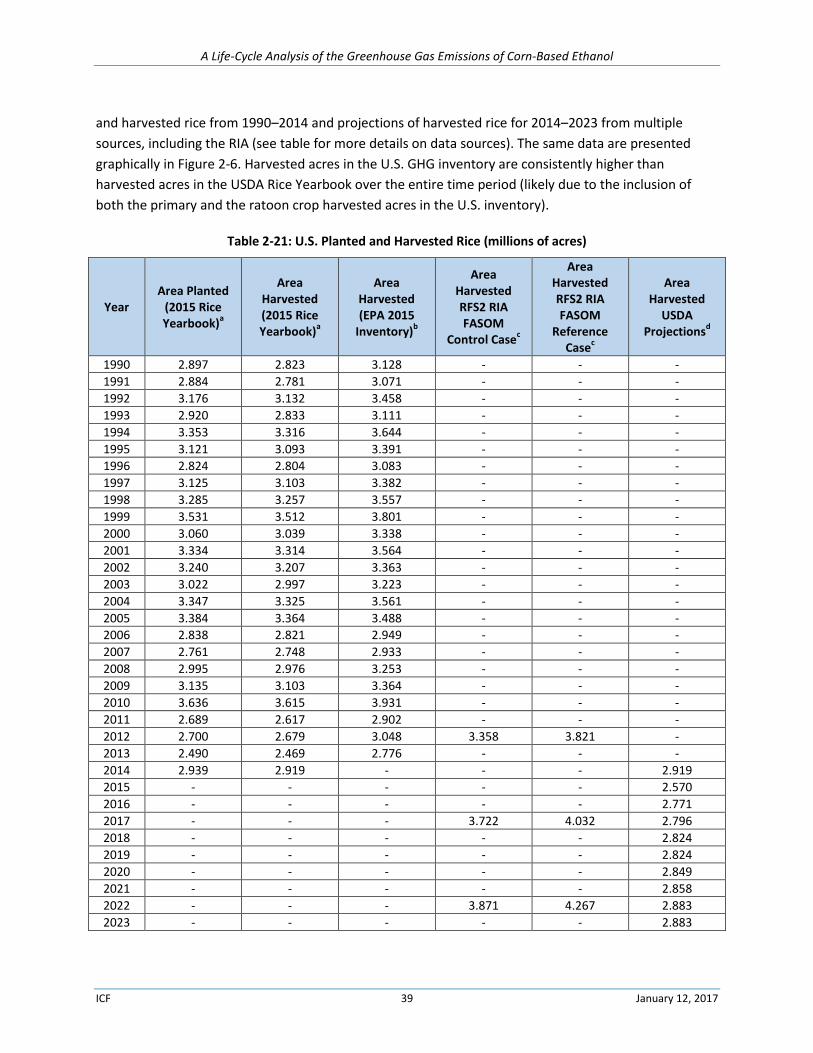
A Life-Cycle Analysis of the Greenhouse Gas Emissions of Corn-Based Ethanol
ICF 39 January 12, 2017
and harvested rice from 1990–2014 and projections of harvested rice for 2014–2023 from multiple
sources, including the RIA (see table for more details on data sources). The same data are presented
graphically in Figure 2-6. Harvested acres in the U.S. GHG inventory are consistently higher than
harvested acres in the USDA Rice Yearbook over the entire time period (likely due to the inclusion of
both the primary and the ratoon crop harvested acres in the U.S. inventory).
Table 2-21: U.S. Planted and Harvested Rice (millions of acres)
Year Area Planted
(2015 Rice Yearbook)
a
Area Harvested (2015 Rice Yearbook)
a
Area Harvested (EPA 2015
Inventory)b
Area Harvested RFS2 RIA FASOM
Control Casec
Area Harvested RFS2 RIA FASOM
Reference Case
c
Area Harvested
USDA Projections
d
1990 2.897 2.823 3.128 - - -
1991 2.884 2.781 3.071 - - -
1992 3.176 3.132 3.458 - - -
1993 2.920 2.833 3.111 - - -
1994 3.353 3.316 3.644 - - -
1995 3.121 3.093 3.391 - - -
1996 2.824 2.804 3.083 - - -
1997 3.125 3.103 3.382 - - -
1998 3.285 3.257 3.557 - - -
1999 3.531 3.512 3.801 - - -
2000 3.060 3.039 3.338 - - -
2001 3.334 3.314 3.564 - - -
2002 3.240 3.207 3.363 - - -
2003 3.022 2.997 3.223 - - -
2004 3.347 3.325 3.561 - - -
2005 3.384 3.364 3.488 - - -
2006 2.838 2.821 2.949 - - -
2007 2.761 2.748 2.933 - - -
2008 2.995 2.976 3.253 - - -
2009 3.135 3.103 3.364 - - -
2010 3.636 3.615 3.931 - - -
2011 2.689 2.617 2.902 - - -
2012 2.700 2.679 3.048 3.358 3.821 -
2013 2.490 2.469 2.776 - - -
2014 2.939 2.919 - - - 2.919
2015 - - - - - 2.570
2016 - - - - - 2.771
2017 - - - 3.722 4.032 2.796
2018 - - - - - 2.824
2019 - - - - - 2.824
2020 - - - - - 2.849
2021 - - - - - 2.858
2022 - - - 3.871 4.267 2.883
2023 - - - - - 2.883
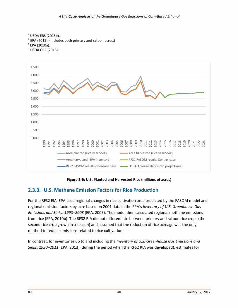
A Life-Cycle Analysis of the Greenhouse Gas Emissions of Corn-Based Ethanol
ICF 40 January 12, 2017
a USDA ERS (2015b).
b EPA (2015). (Includes both primary and ratoon acres.)
c EPA (2010a).
d USDA OCE (2016).
Figure 2-6: U.S. Planted and Harvested Rice (millions of acres)
2.3.3. U.S. Methane Emission Factors for Rice Production
For the RFS2 EIA, EPA used regional changes in rice cultivation area predicted by the FASOM model and
regional emission factors by acre based on 2001 data in the EPA’s Inventory of U.S. Greenhouse Gas
Emissions and Sinks: 1990–2003 (EPA, 2005). The model then calculated regional methane emissions
from rice (EPA, 2010b). The RFS2 RIA did not differentiate between primary and ratoon rice crops (the
second rice crop grown in a season) and assumed that the reduction of rice acreage was the only
method to reduce emissions related to rice cultivation.
In contrast, for inventories up to and including the Inventory of U.S. Greenhouse Gas Emissions and
Sinks: 1990–2011 (EPA, 2013) (during the period when the RFS2 RIA was developed), estimates for
0.000
0.500
1.000
1.500
2.000
2.500
3.000
3.500
4.000
4.500
19
90
19
91
19
92
19
93
19
94
19
95
19
96
19
97
19
98
19
99
20
00
20
01
20
02
20
03
20
04
20
05
20
06
20
07
20
08
20
09
20
10
20
11
20
12
20
13
20
14
20
15
20
16
20
17
20
18
20
19
20
20
20
21
20
22
20
23
Area planted (rice yearbook) Area harvested (rice yearbook)
Area harvested (EPA inventory) RFS2 FASOM results Control case
RFS2 FASOM results reference case USDA Acreage Harvested projections
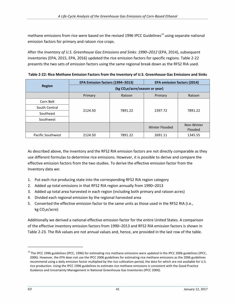
A Life-Cycle Analysis of the Greenhouse Gas Emissions of Corn-Based Ethanol
ICF 41 January 12, 2017
methane emissions from rice were based on the revised 1996 IPCC Guidelines14 using separate national
emission factors for primary and ratoon rice crops.
After the Inventory of U.S. Greenhouse Gas Emissions and Sinks: 1990–2012 (EPA, 2014), subsequent
inventories (EPA, 2015, EPA, 2016) updated the rice emission factors for specific regions. Table 2-22
presents the two sets of emission factors using the same regional break down as the RFS2 RIA used.
Table 2-22: Rice Methane Emission Factors from the Inventory of U.S. Greenhouse Gas Emissions and Sinks
Region EPA Emission factors (1994–2013) EPA emission factors (2014)
(kg CO2e/acre/season or year)
Primary Ratoon Primary Ratoon
Corn Belt
2124.50 7891.22 2397.72 7891.22 South Central
Southeast
Southwest
Winter Flooded Non-Winter
Flooded
Pacific Southwest 2124.50 7891.22 2691.11 1345.55
As described above, the inventory and the RFS2 RIA emission factors are not directly comparable as they
use different formulas to determine rice emissions. However, it is possible to derive and compare the
effective emission factors from the two studies. To derive the effective emission factor from the
Inventory data we:
1. Put each rice producing state into the corresponding RFS2 RIA region category
2. Added up total emissions in that RFS2 RIA region annually from 1990–2013
3. Added up total area harvested in each region (including both primary and ratoon acres)
4. Divided each regional emission by the regional harvested area
5. Converted the effective emission factor to the same units as those used in the RFS2 RIA (i.e.,
kg CO2e/acre)
Additionally we derived a national effective emission factor for the entire United States. A comparison
of the effective inventory emission factors from 1990–2013 and RFS2 RIA emission factors is shown in
Table 2-23. The RIA values are not annual values and, hence, are provided in the last row of the table.
14 The IPCC 1996 guidelines (IPCC, 1996) for estimating rice methane emissions were updated in the IPCC 2006 guidelines (IPCC, 2006). However, the EPA does not use the IPCC 2006 guidelines for estimating rice methane emissions as the 2006 guidelines recommend using a daily emission factor multiplied by the rice cultivation period, the data for which are not available for U.S. rice production. Using the IPCC 1996 guidelines to estimate rice methane emissions is consistent with the Good Practice Guidance and Uncertainty Management in National Greenhouse Gas Inventories (IPCC 2000).
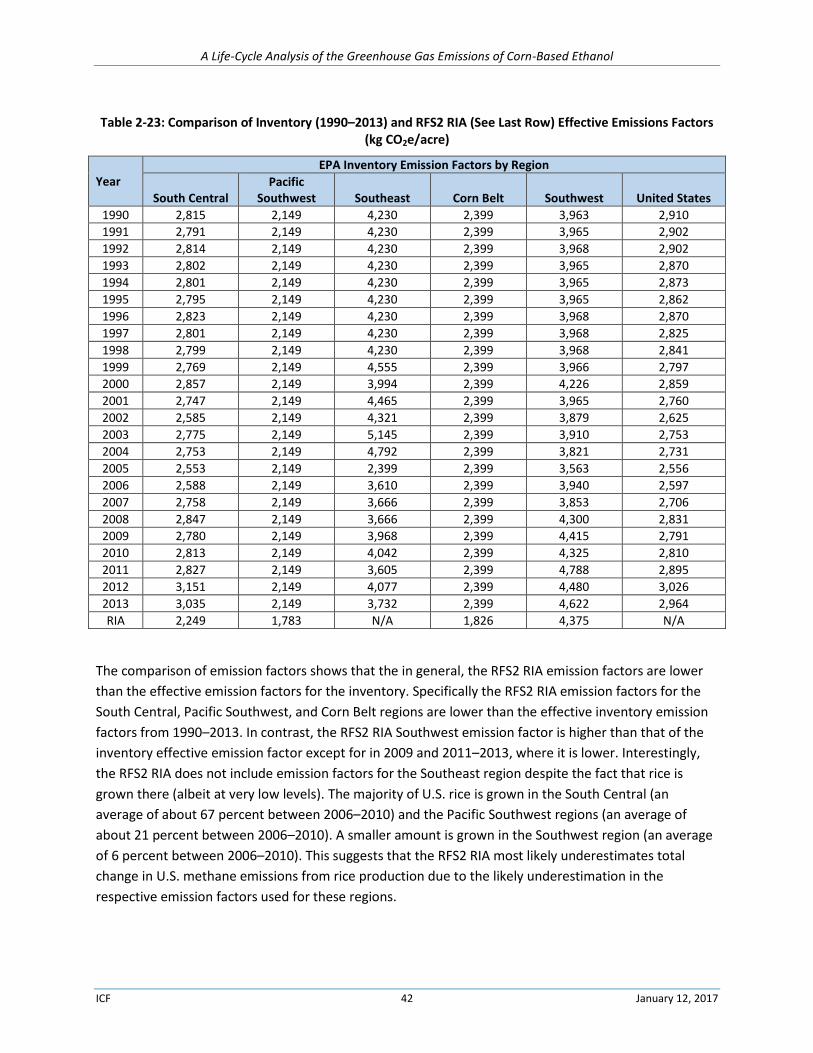
A Life-Cycle Analysis of the Greenhouse Gas Emissions of Corn-Based Ethanol
ICF 42 January 12, 2017
Table 2-23: Comparison of Inventory (1990–2013) and RFS2 RIA (See Last Row) Effective Emissions Factors (kg CO2e/acre)
Year
EPA Inventory Emission Factors by Region
South Central Pacific
Southwest Southeast Corn Belt Southwest United States
1990 2,815 2,149 4,230 2,399 3,963 2,910
1991 2,791 2,149 4,230 2,399 3,965 2,902
1992 2,814 2,149 4,230 2,399 3,968 2,902
1993 2,802 2,149 4,230 2,399 3,965 2,870
1994 2,801 2,149 4,230 2,399 3,965 2,873
1995 2,795 2,149 4,230 2,399 3,965 2,862
1996 2,823 2,149 4,230 2,399 3,968 2,870
1997 2,801 2,149 4,230 2,399 3,968 2,825
1998 2,799 2,149 4,230 2,399 3,968 2,841
1999 2,769 2,149 4,555 2,399 3,966 2,797
2000 2,857 2,149 3,994 2,399 4,226 2,859
2001 2,747 2,149 4,465 2,399 3,965 2,760
2002 2,585 2,149 4,321 2,399 3,879 2,625
2003 2,775 2,149 5,145 2,399 3,910 2,753
2004 2,753 2,149 4,792 2,399 3,821 2,731
2005 2,553 2,149 2,399 2,399 3,563 2,556
2006 2,588 2,149 3,610 2,399 3,940 2,597
2007 2,758 2,149 3,666 2,399 3,853 2,706
2008 2,847 2,149 3,666 2,399 4,300 2,831
2009 2,780 2,149 3,968 2,399 4,415 2,791
2010 2,813 2,149 4,042 2,399 4,325 2,810
2011 2,827 2,149 3,605 2,399 4,788 2,895
2012 3,151 2,149 4,077 2,399 4,480 3,026
2013 3,035 2,149 3,732 2,399 4,622 2,964
RIA 2,249 1,783 N/A 1,826 4,375 N/A
The comparison of emission factors shows that the in general, the RFS2 RIA emission factors are lower
than the effective emission factors for the inventory. Specifically the RFS2 RIA emission factors for the
South Central, Pacific Southwest, and Corn Belt regions are lower than the effective inventory emission
factors from 1990–2013. In contrast, the RFS2 RIA Southwest emission factor is higher than that of the
inventory effective emission factor except for in 2009 and 2011–2013, where it is lower. Interestingly,
the RFS2 RIA does not include emission factors for the Southeast region despite the fact that rice is
grown there (albeit at very low levels). The majority of U.S. rice is grown in the South Central (an
average of about 67 percent between 2006–2010) and the Pacific Southwest regions (an average of
about 21 percent between 2006–2010). A smaller amount is grown in the Southwest region (an average
of 6 percent between 2006–2010). This suggests that the RFS2 RIA most likely underestimates total
change in U.S. methane emissions from rice production due to the likely underestimation in the
respective emission factors used for these regions.
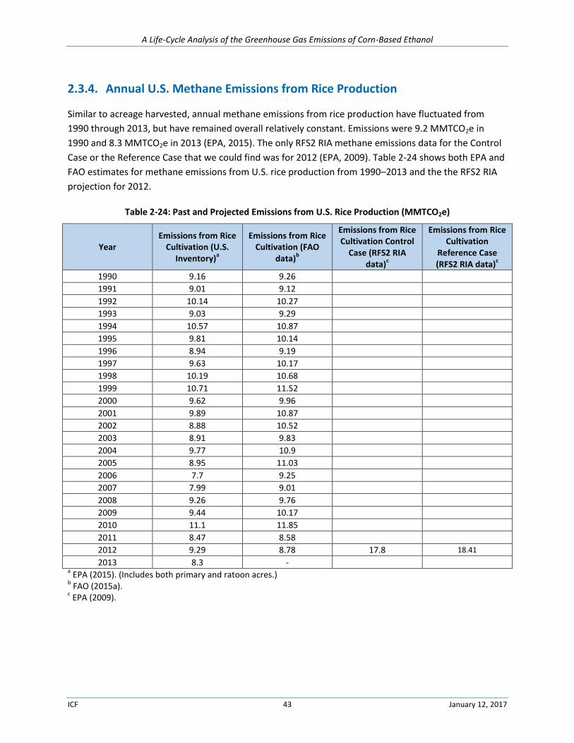
A Life-Cycle Analysis of the Greenhouse Gas Emissions of Corn-Based Ethanol
ICF 43 January 12, 2017
2.3.4. Annual U.S. Methane Emissions from Rice Production
Similar to acreage harvested, annual methane emissions from rice production have fluctuated from
1990 through 2013, but have remained overall relatively constant. Emissions were 9.2 MMTCO2e in
1990 and 8.3 MMTCO2e in 2013 (EPA, 2015). The only RFS2 RIA methane emissions data for the Control
Case or the Reference Case that we could find was for 2012 (EPA, 2009). Table 2-24 shows both EPA and
FAO estimates for methane emissions from U.S. rice production from 1990–2013 and the the RFS2 RIA
projection for 2012.
Table 2-24: Past and Projected Emissions from U.S. Rice Production (MMTCO2e)
Year Emissions from Rice
Cultivation (U.S. Inventory)
a
Emissions from Rice Cultivation (FAO
data)b
Emissions from Rice Cultivation Control
Case (RFS2 RIA data)
c
Emissions from Rice Cultivation
Reference Case (RFS2 RIA data)
c
1990 9.16 9.26
1991 9.01 9.12
1992 10.14 10.27
1993 9.03 9.29
1994 10.57 10.87
1995 9.81 10.14
1996 8.94 9.19
1997 9.63 10.17
1998 10.19 10.68
1999 10.71 11.52
2000 9.62 9.96
2001 9.89 10.87
2002 8.88 10.52
2003 8.91 9.83
2004 9.77 10.9
2005 8.95 11.03
2006 7.7 9.25
2007 7.99 9.01
2008 9.26 9.76
2009 9.44 10.17
2010 11.1 11.85
2011 8.47 8.58
2012 9.29 8.78 17.8 18.41
2013 8.3 -
a EPA (2015). (Includes both primary and ratoon acres.)
b FAO (2015a).
c EPA (2009).
A Life-Cycle Analysis of the Greenhouse Gas Emissions of Corn-Based Ethanol
ICF 44 January 12, 2017
The data show that FAO emissions projections15 are slightly higher than EPA inventory data for all
historic years except for 2012 where the FAO emissions projections are slightly lower than those from
the EPA inventory. The total projected 2012 rice methane emissions from the RFS2 RIA are nearly
double those of the EPA inventory and the FAO, despite the fact that the RFS2 RIA has lower emission
factors than the EPA inventory. The RFS2 RIA estimated 2012 emissions are 17.8 MMT CO2e for the
Control Case and 18.41 MMT CO2e for the Reference Case compared to 9.29 MMT CO2e from the EPA
inventory and 8.78 MMT CO2e from the FAO. The RFS2 RIA values seem high given the RFS2 RIA
estimated acreage and the RFS2 RIA emission factors used. However, as the RFS2 RIA did not provide all
the data used to create the total emissions numbers, we cannot evaluate the underlying assumptions or
data used to develop emission values used in the RFS2 RIA to compare values to updated data.
2.3.5. Conclusions
A review of the current literature shows that U.S. rice production and corresponding methane emissions
have remained relatively constant between 1990 through 2013 despite the expansion in corn and corn
ethanol production. Harvested acres of rice have fluctuated between approximately 2.5 and 3.6 million
acres, and emissions have fluctuated between 7.7 and 11.1 MMTCO2e during this period (USDA ERS,
2015; EPA, 2015). In comparison with the EPA inventory data, the RFS2 RIA FASOM data overestimates
harvested rice acreage in 2012 and underestimates rice emission factors in most regions, when
compared to effective emissions factors from the EPA inventory between 1990 and 2013. However, the
RFS2 RIA total projected 2012 rice methane emissions are nearly double those of the EPA inventory and
the FAO, despite the lower emission factors in the RFS2 RIA.
2.3.6. References: Domestic Rice Methane
EPA, 2015. Inventory of U.S. Greenhouse Gas Emissions and Sinks: 1990–2013. U.S. Environmental Protection Agency. EPA 430-R-15-004. http://www3.epa.gov/climatechange/Downloads/ghgemissions/US-GHG-Inventory-2015-Main-Text.pdf
EPA, 2014. Inventory of U.S. Greenhouse Gas Emissions and Sinks: 1990–2012. U.S. Environmental Protection Agency. EPA 430-R-14-003. http://www3.epa.gov/climatechange/Downloads/ghgemissions/US-GHG-Inventory-2014-Main-Text.pdf
EPA, 2013. Inventory of U.S. Greenhouse Gas Emissions and Sinks: 1990–2011. U.S. Environmental Protection Agency. EPA 430-R-13-001. http://www3.epa.gov/climatechange/Downloads/ghgemissions/US-GHG-Inventory-2013-Main-Text.pdf
15 FAO country emissions are computed at Tier 1 following the Revised 1996 IPCC Guidelines for National GHG Inventories
(IPCC, 1997) and the IPCC 2000 Good Practice Guidance and Uncertainty Management in National GHG Inventories (IPCC, 2000); available by country, with global coverage and relative to the period 1961-present, with annual updates, and projections for 2030 and 2050. (FAO, 2015b).
A Life-Cycle Analysis of the Greenhouse Gas Emissions of Corn-Based Ethanol
ICF 45 January 12, 2017
EPA, 2010b. Life Cycle Analysis Results found in spreadsheet “Forest_Agricultural_Sector_Optimization_Model_(FASOM)_Results_for_Lifecycle_Greenhouse_Gas_(GHG)” Docket ID: EPA-HQ-OAR-2005-0161-0948. Available online at: http://www.regulations.gov/#!documentDetail;D=EPA-HQ-OAR-2005-0161-0948
EPA, 2010a. Renewable Fuel Standard (RFS2) Final Regulatory Impact Analysis. EPA-420-R-10-006. Available: http://www3.epa.gov/otaq/renewablefuels/420r10006.pdf
EPA, 2009. GREET1.8c Results found in spreadsheet, “Renewable Fuel Lifecycle Greenhouse Gas Calculations.xls” (Docket ID: EPA-HQ-OAR-2005-0161-0950). Available online at: http://www.regulations.gov/#!documentDetail;D=EPA-HQ-OAR-2005-0161-0950
EPA, 2005. Inventory of U.S. Greenhouse Gas Emissions and Sinks: 1990-2003. U.S. Environmental Protection Agency. EPA 430-R-05-003. http://www3.epa.gov/climatechange/Downloads/ghgemissions/05CR.pdf
FAO, 2015a. FAOSTAT, Emissions – Agriculture. Food and Agriculture Organization of the United Nations, Stastics Division. Accessed January 20, 2016. http://faostat3.fao.org/browse/G1/*/E
FAO, 2015b. Emissions- Agriculture: Rice cultivation. Food and Agriculture Organization of the United Nations. Accessed 1/20/16 http://faostat3.fao.org/mes/methodology_list/E
Gathorne-Hardy, A. (2013). Greenhouse gas emissions from rice (Vol. 3). RGTW Working Paper no. 3 http://www.southasia.ox.ac.uk/sites/sias/files/documents/GHG%20emissions%20from%20rice%20-%20%20working%20paper.pdf
Hussain, S., Peng, S., Fahad, S., Khaliq, A., Huang, J., Cui, K., & Nie, L. (2015). Rice management interventions to mitigate greenhouse gas emissions: a review. Environmental Science and Pollution Research, 22(5), 3342-3360.
IPCC, 2006. 2006 IPCC Guidelines for National Greenhouse Gas Inventories. Intergovernmental Panel on Climate Change. National Greenhouse Gas Inventories Programme, Kanagawa, Japan. http://www.ipcc-nggip.iges.or.jp/public/2006gl/
IPCC, 2000. IPCC (2000) Good Practice Guidance and Uncertainty Management in National Greenhouse Gas Inventories. Intergovernmental Panel on Climate Change. National Greenhouse Gas Inventories Programme, Kanagawa, Japan. http://www.ipcc-nggip.iges.or.jp/public/gp/english/
IPCC, 1997. Revised 1996 IPCC Guidelines for National Greenhouse Gas Inventories. Intergovernmental Panel on Climate Change. National Greenhouse Gas Inventories Programme, Kanagawa, Japan. http://www.ipcc-nggip.iges.or.jp/public/gl/invs1.html
USDA, ERS, 2015a. Rice Yearbook 2015, Table 7: State and U.S. rice acreage, yield, and production, all rice and by class. U.S. Department of Agriculture, Economic Research Service. http://www.ers.usda.gov/data-products/rice-yearbook-2015.aspx
USDA, ERS, 2015b. Rice Yearbook 2015, Table 9: U.S. rice acreage, yield, and production. U.S. Department of Agriculture, Economic Research Service. http://www.ers.usda.gov/data-products/rice-yearbook-2015.aspx
USDA OCE, 2013a. United States: Rice, Agricultural Weather Assessments. U.S. Department of Agriculture, Office of the Chief Economist, World Agricultural Outlook Board. http://www.usda.gov/oce/weather/pubs/Other/MWCACP/Graphs/USA/US_Rice.pdf
A Life-Cycle Analysis of the Greenhouse Gas Emissions of Corn-Based Ethanol
ICF 46 January 12, 2017
USDA OCE, 2013b. United States: Corn, Agricultural Weather Assessments. U.S. Department of Agriculture, Office of the Chief Economist, World Agricultural Outlook Board. http://www.usda.gov/oce/weather/pubs/Other/MWCACP/Graphs/USA/US_Corn.pdf
USDA OCE, 2016. USDA Agricultural Projections to 2025. “U.S. rice” http://www.usda.gov/oce/commodity/projections/Rice.xls
2.4. Domestic and International Livestock
Aligned with EPA’s final Regulatory Impact Analysis (RIA) (EPA, 2010a) for the revised Renewable Fuel
Standard Program (RFS2), the Domestic and International Livestock emission categories includes
emissions, both domestically and internationally, related to domestic corn ethanol production and
livestock production systems. Internationally we summarize the literature related to emissions
associated with livestock production systems in various regions with whom the United States has
significant agricultural and energy trade. Impacts internationally are projected to vary by livestock and
ethanol feedstock (corn, soy, sugarcane, and switchgrass).
Livestock production systems include practices that involve raising livestock for meat, eggs, dairy, and
other products such as leather, fur, and wool. Farmers and other facility operators raise animals in
either confined, semi-confined, or unconfined spaces. Literature incorporated into this review is mostly
limited to considering variables related to corn ethanol production, such as changes in livestock
production that affect the cultivation and use of corn, including use of corn-based feed (including
distillers grains), land-use demands for domestic livestock production (range, feedlots, pasture), trends
in typical animal mass (TAM), total population, and the amount of meat and dairy from each animal.
The international livestock sector is characterized by a dichotomy between developing and developed
countries. Much of the growth in total meat production between 1980 and 2002 was concentrated in
countries with rapid economic growth. In developed countries, production and consumption of livestock
products are growing slowly or not at all. Livestock production in industrialized countries accounts for 53
percent of agricultural GDP (Thornton, 2010). Particularly of interest are the practices in South America.
The continent’s livestock industry (especially swine and cattle production) is concentrated in Brazil and is
characterized by landless monogastric production systems (LLM) and Grassland-based livestock
production systems (Roman et al., 2006).
2.4.1. Livestock Emission Sources
Although there are emissions associated with livestock production that are not directly emitted from
livestock and their waste (such as due to transportation, animal feed production, or dairy/meat
processing), this literature review focuses on the two primary sources of emissions from livestock
included in the RFS2 RIA: enteric fermentation and manure management. Enteric fermentation
produces methane (“enteric CH4”) and manure management practices result in emissions of CH4 and
nitrous oxide (N2O).
A Life-Cycle Analysis of the Greenhouse Gas Emissions of Corn-Based Ethanol
ICF 47 January 12, 2017
2.4.1.1. Enteric Fermentation
Enteric fermentation is a process through which microbes present in the digestive tract of livestock
break down food, emitting CH4 as a by-product. Ruminant animals, such as cattle, sheep, and goats,
have multi-chambered digestive systems that produce more CH4 than those of non-ruminant animals.
Methane emissions are also produced by monogastric (non-ruminant, e.g., swine) livestock but at a
magnitude much lower than for ruminant livestock.
Methane emissions from enteric fermentation depend on a combination of the following factors:
predominant animal types, the quantity and quality of the diet, use of dietary additives, and the animals’
activity data (e.g., work performed, pregnancy rates) (ICF International, 2013; Eve et al., 2014).
The literature also indicates that a significant component in determining enteric emissions is dietary
composition, which consists of overall feed intake and feed composition. For example, digestible energy
(DE) in low-quality feed such as late-season forage is less than that in high-quality feed (e.g., mixed feed
or spring forage). With lower quality food sources, cattle will need to eat more food in order to get the
same amount of energy, thus leading to greater emissions in most cases. Increasing the ratio of grains
(and other concentrates) to forage; increasing dietary fat content; and additives can decrease enteric
CH4 emissions from cattle (ICF International, 2013; Eve et al., 2014; Gerber et al., 2013). Diets rich in
biofuel crop residues like distillers grains can have a higher fat content, helping to reduce enteric
emissions from cattle (Lemenager et al., 2006; Latour and Schinckel, 2007). Expansion of the ethanol
industry led to increased demand for corn and an increased supply of co-products from the ethanol
production processes (USDA, 2009). Ethanol co-products have the potential to serve as both an
economic source of cattle feed (USDA, 2009) and a means to reduce enteric emissions. However, the
inclusion of additives, such as ionophores, nitrates, and tannins, have unclear long-term benefits in
terms of reducing enteric CH4 emissions.
At least one study concludes that cattle consuming steam-flaked corn (SFC)-based diets produce less
enteric CH4 and preserve more energy than cattle that consume dry-rolled corn (DRC)-based diets.
However, inclusion of wet distillers grains with solubles (WDGS) at 30 percent of feed composition has
little effect on enteric CH4 production and energy metabolism (Hales et al., 2012). Another study
concludes that, compared with use of WDGS, using corn or wheat based DDGs in finishing cattle’s diets
reduced enteric CH4 emissions by 1 percent and 0.8 percent, respectively (Wunerberg et al., 2013).
Cows in intensive dairy production systems are typically fed high ratios of forages to concentrates. Feed
often includes corn silage, alfalfa/ grass silage, alfalfa hay, high-moisture corn, soybean meal, and
sometimes commodity feeds (e.g., corn gluten and/or dried distillers grains (DDG)). Dairy cows are fed
diets that support the relevant milk production stage (ICF International, 2013). Although dairy cows are
fed high quality nutrition, linked to lower enteric CH4 emissions than lower-quality nutrition, they have a
much higher TAM than beef cattle in the United States (EPA, 2015).
A Life-Cycle Analysis of the Greenhouse Gas Emissions of Corn-Based Ethanol
ICF 48 January 12, 2017
2.4.1.2. Manure Management
Manure management is the collection, storage, transfer, and treatment of animal urine and feces (Eve
et al., 2014). The anaerobic decomposition of manure results in CH4 production and both direct and
indirect pathways16 results in N2O emissions. Manure management systems include variations within the
following categories: solid storage, slurry systems, lagoons, and spreading.
The amount of CH4 and N2O generated from manure management practices depends on the animal
type, animal diet, and activity data. However, the primary determinant of manure management GHG
emissions is the system used to manage manure (e.g., solid storage, anaerobic lagoons, ponds). The
same quantity of manure will generate different CH4 and N2O emissions as the management practice
defines the emission rate (ICF International, 2013; Eve et al., 2014; Gerber et al., 2013). Manure stored
under anaerobic conditions produce a significant portion of all manure-related emissions (specifically, as
CH4), so covering anaerobic lagoons or utilizing other anaerobic digesters provides a good opportunity to
reduce these emissions (ICF International, 2013; Gerber et al., 2013).
2.4.2. Domestic Livestock Emissions
Overall emissions from domestic livestock production are dominated by enteric CH4, but manure
management practices produce emissions that are still a significant component of total agricultural
sector emissions. Enteric CH4 is more closely linked to diet, and thus corn (and other grain) production,
than are the GHGs produced by manure management. Manure management mitigation methods focus
primarily on capturing existing emissions, rather than through dietary modification.
2.4.2.1. Domestic Livestock Enteric Fermentation Emissions
In 2014, enteric CH4 emissions in the United States were 164.3 MMT CO2e, (i.e., more than 65 percent of
the emissions from animal production systems). More than 71 percent was from beef cattle and more
than 96 percent was from beef and dairy cattle together (EPA, 2016). Enteric CH4 is the primary GHG
produced by dairy cows (on a per-head basis). However, there are more beef cattle than dairy cows in
the United States, consequently, more overall enteric CH4 is produced by beef cattle (ICF International,
2013).
The model used in the RFS2 RIA (FASOM) projects domestic enteric CH4 emissions using 2001 average
emissions per head according to the Inventory of U.S. Greenhouse Gas Emissions and Sinks: 1990–2003
(EPA, 2005) and multiplying them by the projected change in populations. Therefore, emissions are
based only on populations, trends for which are discussed in Section 2.4.2.3.
16 Indirect routes for producing N2O include: (1) the direct production of NH3 and NOx later reacting further to produce N2O and (2) runoff and leaching of N from manure into groundwater, also eventually reacting further to produce N2O (Eve et al., 2014; EPA, 2015).
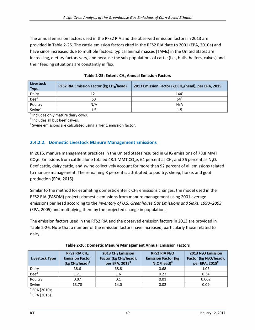
A Life-Cycle Analysis of the Greenhouse Gas Emissions of Corn-Based Ethanol
ICF 49 January 12, 2017
The annual emission factors used in the RFS2 RIA and the observed emission factors in 2013 are
provided in Table 2-25. The cattle emission factors cited in the RFS2 RIA date to 2001 (EPA, 2010a) and
have since increased due to multiple factors: typical animal masses (TAMs) in the United States are
increasing, dietary factors vary, and because the sub-populations of cattle (i.e., bulls, heifers, calves) and
their feeding situations are constantly in flux.
Table 2-25: Enteric CH4 Annual Emission Factors
Livestock Type
RFS2 RIA Emission Factor (kg CH4/head) 2013 Emission Factor (kg CH4/head), per EPA, 2015
Dairy 121 144a
Beef 53 64b
Poultry N/A N/A
Swinec 1.5 1.5
a Includes only mature dairy cows.
b Includes all but beef calves.
c Swine emissions are calculated using a Tier 1 emission factor.
2.4.2.2. Domestic Livestock Manure Management Emissions
In 2015, manure management practices in the United States resulted in GHG emissions of 78.8 MMT
CO2e. Emissions from cattle alone totaled 48.1 MMT CO2e, 64 percent as CH4 and 36 percent as N2O.
Beef cattle, dairy cattle, and swine collectively account for more than 92 percent of all emissions related
to manure management. The remaining 8 percent is attributed to poultry, sheep, horse, and goat
production (EPA, 2015).
Similar to the method for estimating domestic enteric CH4 emissions changes, the model used in the
RFS2 RIA (FASOM) projects domestic emissions from manure management using 2001 average
emissions per head according to the Inventory of U.S. Greenhouse Gas Emissions and Sinks: 1990–2003
(EPA, 2005) and multiplying them by the projected change in populations.
The emission factors used in the RFS2 RIA and the observed emission factors in 2013 are provided in
Table 2-26. Note that a number of the emission factors have increased, particularly those related to
dairy.
Table 2-26: Domestic Manure Management Annual Emission Factors
Livestock Type RFS2 RIA CH4
Emission Factor (kg CH4/head)
a
2013 CH4 Emission Factor (kg CH4/head),
per EPA, 2015b
RFS2 RIA N2O Emission Factor (kg
N2O/head)a
2013 N2O Emission Factor (kg N2O/head),
per EPA, 2015b
Dairy 38.6 68.8 0.68 1.03
Beef 1.71 1.6 0.23 0.34
Poultry 0.07 0.1 0.01 0.002
Swine 13.78 14.0 0.02 0.09 a EPA (2010);
b EPA (2015).
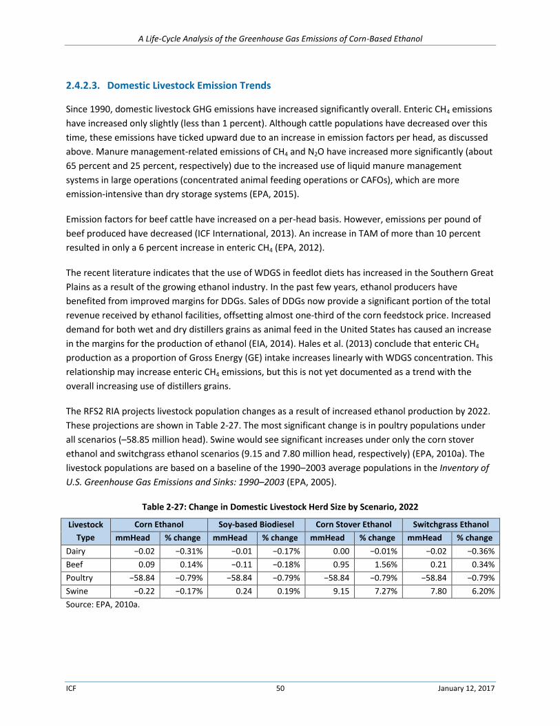
A Life-Cycle Analysis of the Greenhouse Gas Emissions of Corn-Based Ethanol
ICF 50 January 12, 2017
2.4.2.3. Domestic Livestock Emission Trends
Since 1990, domestic livestock GHG emissions have increased significantly overall. Enteric CH4 emissions
have increased only slightly (less than 1 percent). Although cattle populations have decreased over this
time, these emissions have ticked upward due to an increase in emission factors per head, as discussed
above. Manure management-related emissions of CH4 and N2O have increased more significantly (about
65 percent and 25 percent, respectively) due to the increased use of liquid manure management
systems in large operations (concentrated animal feeding operations or CAFOs), which are more
emission-intensive than dry storage systems (EPA, 2015).
Emission factors for beef cattle have increased on a per-head basis. However, emissions per pound of
beef produced have decreased (ICF International, 2013). An increase in TAM of more than 10 percent
resulted in only a 6 percent increase in enteric CH4 (EPA, 2012).
The recent literature indicates that the use of WDGS in feedlot diets has increased in the Southern Great
Plains as a result of the growing ethanol industry. In the past few years, ethanol producers have
benefited from improved margins for DDGs. Sales of DDGs now provide a significant portion of the total
revenue received by ethanol facilities, offsetting almost one-third of the corn feedstock price. Increased
demand for both wet and dry distillers grains as animal feed in the United States has caused an increase
in the margins for the production of ethanol (EIA, 2014). Hales et al. (2013) conclude that enteric CH4
production as a proportion of Gross Energy (GE) intake increases linearly with WDGS concentration. This
relationship may increase enteric CH4 emissions, but this is not yet documented as a trend with the
overall increasing use of distillers grains.
The RFS2 RIA projects livestock population changes as a result of increased ethanol production by 2022.
These projections are shown in Table 2-27. The most significant change is in poultry populations under
all scenarios (–58.85 million head). Swine would see significant increases under only the corn stover
ethanol and switchgrass ethanol scenarios (9.15 and 7.80 million head, respectively) (EPA, 2010a). The
livestock populations are based on a baseline of the 1990–2003 average populations in the Inventory of
U.S. Greenhouse Gas Emissions and Sinks: 1990–2003 (EPA, 2005).
Table 2-27: Change in Domestic Livestock Herd Size by Scenario, 2022
Livestock
Type
Corn Ethanol Soy-based Biodiesel Corn Stover Ethanol Switchgrass Ethanol
mmHead % change mmHead % change mmHead % change mmHead % change
Dairy −0.02 −0.31% −0.01 −0.17% 0.00 −0.01% −0.02 −0.36%
Beef 0.09 0.14% −0.11 −0.18% 0.95 1.56% 0.21 0.34%
Poultry −58.84 −0.79% −58.84 −0.79% −58.84 −0.79% −58.84 −0.79%
Swine −0.22 −0.17% 0.24 0.19% 9.15 7.27% 7.80 6.20%
Source: EPA, 2010a.
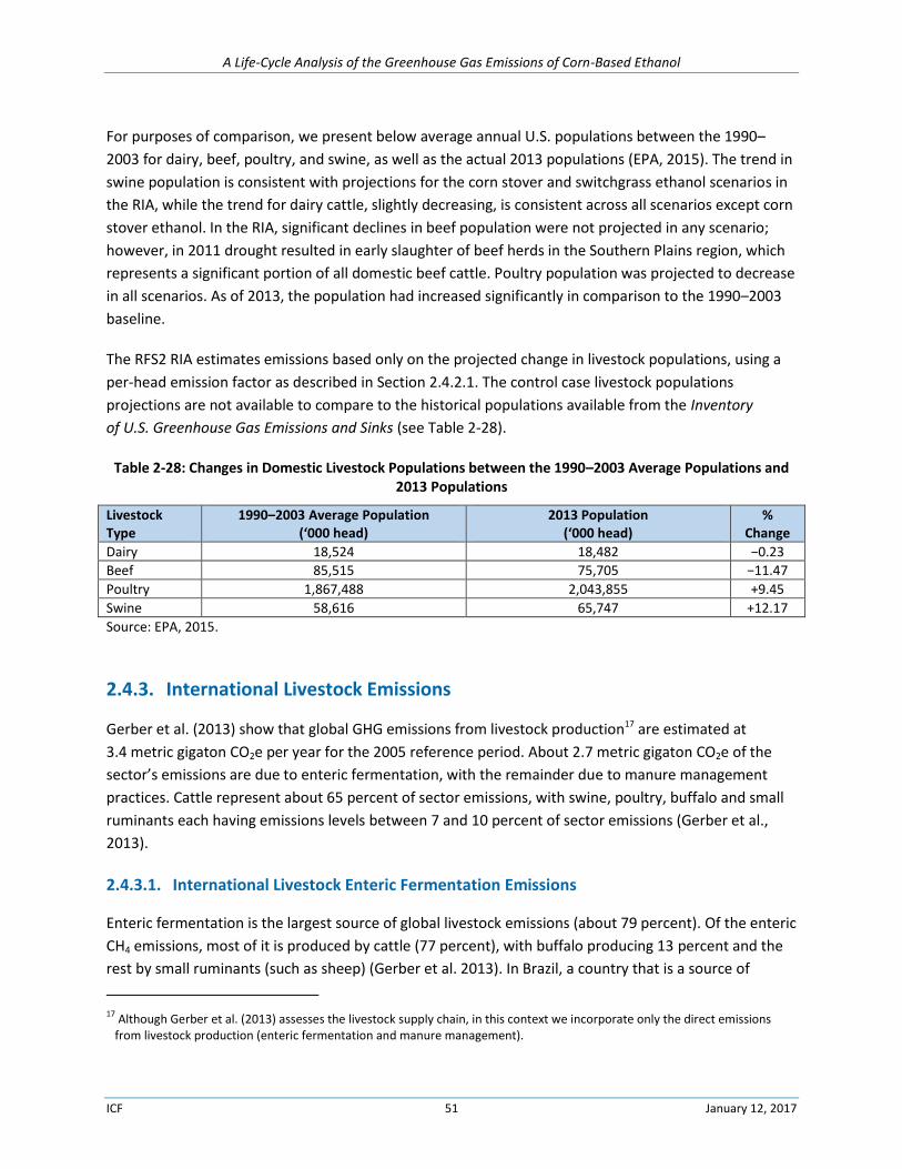
A Life-Cycle Analysis of the Greenhouse Gas Emissions of Corn-Based Ethanol
ICF 51 January 12, 2017
For purposes of comparison, we present below average annual U.S. populations between the 1990–
2003 for dairy, beef, poultry, and swine, as well as the actual 2013 populations (EPA, 2015). The trend in
swine population is consistent with projections for the corn stover and switchgrass ethanol scenarios in
the RIA, while the trend for dairy cattle, slightly decreasing, is consistent across all scenarios except corn
stover ethanol. In the RIA, significant declines in beef population were not projected in any scenario;
however, in 2011 drought resulted in early slaughter of beef herds in the Southern Plains region, which
represents a significant portion of all domestic beef cattle. Poultry population was projected to decrease
in all scenarios. As of 2013, the population had increased significantly in comparison to the 1990–2003
baseline.
The RFS2 RIA estimates emissions based only on the projected change in livestock populations, using a
per-head emission factor as described in Section 2.4.2.1. The control case livestock populations
projections are not available to compare to the historical populations available from the Inventory
of U.S. Greenhouse Gas Emissions and Sinks (see Table 2-28).
Table 2-28: Changes in Domestic Livestock Populations between the 1990–2003 Average Populations and 2013 Populations
Livestock Type
1990–2003 Average Population (‘000 head)
2013 Population (‘000 head)
% Change
Dairy 18,524 18,482 −0.23
Beef 85,515 75,705 −11.47
Poultry 1,867,488 2,043,855 +9.45
Swine 58,616 65,747 +12.17
Source: EPA, 2015.
2.4.3. International Livestock Emissions
Gerber et al. (2013) show that global GHG emissions from livestock production17 are estimated at
3.4 metric gigaton CO2e per year for the 2005 reference period. About 2.7 metric gigaton CO2e of the
sector’s emissions are due to enteric fermentation, with the remainder due to manure management
practices. Cattle represent about 65 percent of sector emissions, with swine, poultry, buffalo and small
ruminants each having emissions levels between 7 and 10 percent of sector emissions (Gerber et al.,
2013).
2.4.3.1. International Livestock Enteric Fermentation Emissions
Enteric fermentation is the largest source of global livestock emissions (about 79 percent). Of the enteric
CH4 emissions, most of it is produced by cattle (77 percent), with buffalo producing 13 percent and the
rest by small ruminants (such as sheep) (Gerber et al. 2013). In Brazil, a country that is a source of
17 Although Gerber et al. (2013) assesses the livestock supply chain, in this context we incorporate only the direct emissions from livestock production (enteric fermentation and manure management).
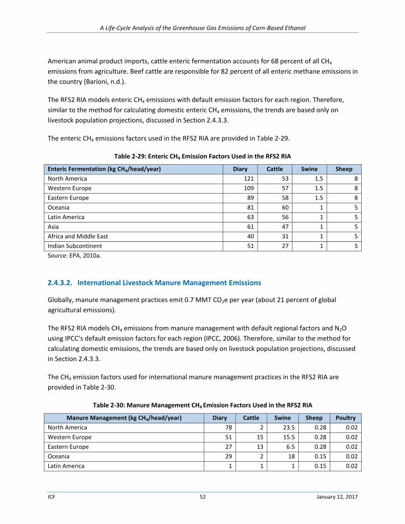
A Life-Cycle Analysis of the Greenhouse Gas Emissions of Corn-Based Ethanol
ICF 52 January 12, 2017
American animal product imports, cattle enteric fermentation accounts for 68 percent of all CH4
emissions from agriculture. Beef cattle are responsible for 82 percent of all enteric methane emissions in
the country (Barioni, n.d.).
The RFS2 RIA models enteric CH4 emissions with default emission factors for each region. Therefore,
similar to the method for calculating domestic enteric CH4 emissions, the trends are based only on
livestock population projections, discussed in Section 2.4.3.3.
The enteric CH4 emissions factors used in the RFS2 RIA are provided in Table 2-29.
Table 2-29: Enteric CH4 Emission Factors Used in the RFS2 RIA
Enteric Fermentation (kg CH4/head/year) Diary Cattle Swine Sheep
North America 121 53 1.5 8
Western Europe 109 57 1.5 8
Eastern Europe 89 58 1.5 8
Oceania 81 60 1 5
Latin America 63 56 1 5
Asia 61 47 1 5
Africa and Middle East 40 31 1 5
Indian Subcontinent 51 27 1 5
Source: EPA, 2010a.
2.4.3.2. International Livestock Manure Management Emissions
Globally, manure management practices emit 0.7 MMT CO2e per year (about 21 percent of global
agricultural emissions).
The RFS2 RIA models CH4 emissions from manure management with default regional factors and N2O
using IPCC’s default emission factors for each region (IPCC, 2006). Therefore, similar to the method for
calculating domestic emissions, the trends are based only on livestock population projections, discussed
in Section 2.4.3.3.
The CH4 emission factors used for international manure management practices in the RFS2 RIA are
provided in Table 2-30.
Table 2-30: Manure Management CH4 Emission Factors Used in the RFS2 RIA
Manure Management (kg CH4/head/year) Diary Cattle Swine Sheep Poultry
North America 78 2 23.5 0.28 0.02
Western Europe 51 15 15.5 0.28 0.02
Eastern Europe 27 13 6.5 0.28 0.02
Oceania 29 2 18 0.15 0.02
Latin America 1 1 1 0.15 0.02
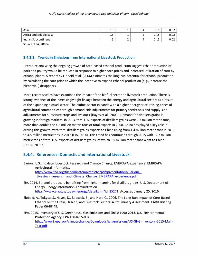
A Life-Cycle Analysis of the Greenhouse Gas Emissions of Corn-Based Ethanol
ICF 53 January 12, 2017
Asia 18 1 4 0.15 0.02
Africa and Middle East 1.5 1 2 0.15 0.02
Indian Subcontinent 5 2 4 0.15 0.02
Source: EPA, 2010a
2.4.3.3. Trends in Emissions from International Livestock Production
Literature analyzing the ongoing growth of corn-based ethanol production suggests that production of
pork and poultry would be reduced in response to higher corn prices and increased utilization of corn by
ethanol plants. A report by Elobeid et al. (2006) estimates the long-run potential for ethanol production
by calculating the corn price at which the incentive to expand ethanol production (e.g., increase the
blend wall) disappears.
More recent studies have examined the impact of the biofuel sector on livestock production. There is
strong evidence of the increasingly tight linkage between the energy and agricultural sectors as a result
of the expanding biofuel sector. The biofuel sector expands with a higher energy price, raising prices of
agricultural commodities through demand-side adjustments for primary feedstocks and supply-side
adjustments for substitute crops and livestock (Hayes et al., 2009). Demand for distillers grains is
growing in foreign markets. In 2013, total U.S. exports of distillers grains were 9.7 million metric tons,
more than double the 4.5 million metric tons of total exports in 2008. China has played a key role in
driving this growth, with total distillers grains exports to China rising from 1.4 million metric tons in 2011
to 4.5 million metric tons in 2013 (EIA, 2014). This trend has continued through 2015 with 12.7 million
metric tons of total U.S. exports of distillers grains, of which 6.5 million metric tons went to China
(USDA, 2016b).
2.4.4. References: Domestic and International Livestock
Barioni, L.G., no date. Livestock Research and Climate Change, EMBRAPA experience. EMBRAPA Agricultural Informatics. http://www.fao.org/fileadmin/templates/tci/pdf/presentations/Barioni_-_Livestock_research_and_Climate_Change_EMBRAPA_experience.pdf
EIA, 2014. Ethanol producers benefiting from higher margins for distillers grains. U.S. Department of Energy, Energy Information Administration https://www.eia.gov/todayinenergy/detail.cfm?id=15271. Accessed January 25, 2016.
Elobeid, A., Tokgoz, S., Hayes, D., Babcock, B., and Hart, C., 2006. The Long-Run Impact of Corn-Based Ethanol on the Grain, Oilseed, and Livestock Sectors: A Preliminary Assessment. CARD Briefing Paper 06-BP 49.
EPA, 2015. Inventory of U.S. Greenhouse Gas Emissions and Sinks: 1990-2013. U.S. Environmental Protection Agency. EPA 430-R-15-004. http://www3.epa.gov/climatechange/Downloads/ghgemissions/US-GHG-Inventory-2015-Main-Text.pdf
A Life-Cycle Analysis of the Greenhouse Gas Emissions of Corn-Based Ethanol
ICF 54 January 12, 2017
EPA, 2012. Operating Anaerobic Digester Projects, U.S. Environmental Protection Agency. http://www.epa.gov/agstar/projects/index.html. Accessed January 21, 2016.
EPA, 2010a. Renewable Fuel Standard (RFS2) Final Regulatory Impact Analysis. EPA-420-R-10-006. Available: http://www3.epa.gov/otaq/renewablefuels/420r10006.pdf
EPA, 2005. Inventory of U.S. Greenhouse Gas Emissions and Sinks: 1990-2003. U.S. Environmental Protection Agency. EPA 430-R-05-003. http://www3.epa.gov/climatechange/Downloads/ghgemissions/05CR.pdf
Eve, M., D. Pape, M. Flugge, R. Steele, D. Man, M. Riley‐Gilbert, and S. Biggar, (Eds), 2014. Quantifying Greenhouse Gas Fluxes in Agriculture and Forestry: Methods for Entity‐Scale Inventory. Technical Bulletin Number 1939. Office of the Chief Economist, U.S. Department of Agriculture, Washington, DC. 606 pages. July 2014.
Gerber, P.J., Steinfeld, H., Henderson, B., Mottet, A., Opio, C., Dijkman, J., Falcucci, A. and Tempio, G., 2013. Tackling climate change through livestock – A global assessment of emissions and mitigation opportunities. Food and Agriculture Organization of the United Nations (FAO), Rome.
Hales, K.E., Cole, N.A., MacDonald, J.C., 2012. Effects of corn processing method and dietary inclusion of wet distillers grains with solubles on energy metabolism, carbon-nitrogen balance, and methane emissions of cattle. Journal of Animal Science, 90(9):3174-85.
Hales, K.E., Cole, N.A., MacDonald, J.C., 2013. Effects of increasing concentrations of wet distillers grains with solubles in steam-flaked, corn-based diets on energy metabolism, carbon-nitrogen balance, and methane emissions of cattle. Journal of Animal Science, 91(2):819-28.
Hayes, D., Babcock, B., Fabiosa, J., Tokgoz, S., Elobeid, A., Yu, T., Dong, F., Hard, C., Chavez, E., Pan, S., Carriquiry, M., and Dumortier, J., 2009. Biofuels: Potential Production Capacity, Effects on Grain and Livestock Sectors, and Implications for Food Prices and Consumers. Journal of Agricultural and Applied Economics, 41(2): 465-491.
Hünerberg, M., McGinn, S.M., Beauchemin, K.A., Okine, E.K., Harstad, O.M., McAllister, T.A., 2013. Effect of dried distillers' grains with solubles on enteric methane emissions and nitrogen excretion from finishing beef cattle. Canadian Journal of Animal Science, 93(3): 373-385.
ICF International, 2013. Greenhouse Gas Mitigation Options and Costs for Agricultural Land and Animal Production within the United States. U.S. Department of Agriculture, Climate Change Program Office.
IPCC, 2006. 2006 IPCC Guidelines for National Greenhouse Gas Inventories. Volume 4, Chapter 10. International Panel on Climate Change. http://www.ipcc-nggip.iges.or.jp/public/2006gl/pdf/4_Volume4/V4_10_Ch10_Livestock.pdf
Latour, M., and Schinckel, A., 2007. The Influence of Dried Distillers’ Grains on Carcass Fat in Swine. BioEnergy (ID-345-W), Department of Animal Sciences, Purdue University. https://www.extension.purdue.edu/extmedia/id/id-345-w.pdf
Lemenager, R., Applegate, T., Claeys, M., Donkin, S., Johnson, T., Lake, S., Neary, M., Radcliffe, S., Richert, B., Schinckel, A., Schutz, M., and Sutton, A. 2006. The Value of Distillers’ Grains as a Livestock Feed. BioEnergy (ID-330), Department of Animal Sciences, Purdue University. https://www.extension.purdue.edu/extmedia/id/id-330.pdf
A Life-Cycle Analysis of the Greenhouse Gas Emissions of Corn-Based Ethanol
ICF 55 January 12, 2017
Robinson, T.P., Thornton P.K., Franceschini, G., Kruska, R.L., Chiozza, F., Notenbaert, A., Cecchi, G., Herrero, M., Epprecht, M., Fritz, S., You, L., Conchedda, G. and See, L., 2011. Global livestock production systems. Rome, Food and Agriculture Organization of the United Nations (FAO) and International Livestock Research Institute (ILRI), 152 pp.
Roman, A., Lukesova, D., Novak, P., and Zizlavsky, M., 2006. Description of Meat Production in South America. Agrucultura Tropica et Subtropica. Volume 39 (4).
Teenstra, E., Vellinga, T., Aektasaeng, N., Amatayakul, W., Ndambi, A., Pelster, D., Germer, L., Jenet, A., Opio, C., Andeweg, K., 2014. Global Assessment of Manure Management Policies and Practices. Wageningen, Wageningen UR (University & Research centre) Livestock Research, Livestock Research Report 844.
Thornton, P.K., 2010. Livestock Production: Recent Trends, Future Prospects. Philosophical Transactions of the Royal Society. 365(1554): 2853–2867.
USDA ERS, 2009. Ethanol Co-Product Use in U.S. Cattle Feeding. U.S. Department of Agriculture, Economic Research Service. http://www.ers.usda.gov/media/147398/fds09d01.pdf
USDA FAS, 2016. USDA Foreign Agricultural Service Export Sales Reporting Database. Accessed on December 28, 2016. https://apps.fas.usda.gov/gats/ExpressQuery1.aspx
2.5. International Land-Use Change
The FAPRI-CARD model was used to determine the number of hectares that will change internationally
(excluding the United States) based on the impact of RFS2. Based on a review of published literature, it
seems that the land-use patterns that were anticipated, particularly in South America and Africa, have
not materialized.
2.5.1. Activity Data Used in RFS2 RIA
Iowa State University and the Center for Agricultural and Rural Development developed and manage
FAPRI-CARD’s international module. The module is based on multi-market, partial-equilibrium,
econometric, non-spatial models. It considers a number of factors including population and GDP growth;
production and consumption trends; existing trade patterns; and both international and domestic
pricing. The model evaluates grains, oilseeds, livestock, dairy products, sugar and biofuels (ethanol and
biodiesel) across the 54 major producing countries and regions. The area harvested was determined for
each of the countries and regions, however FAPRI-CARD does not predict what type of land will be
affected only the number of acres. EPA’s RFS2 RIA determined the type of land using GIS data. Results
showed that the international crop area harvested changed by 789 thousand hectares for the Corn
Ethanol scenario in 2022.
FAPRI-CARD determined the change in harvested hectares for 20 crops in 2022, as seen below in Figure
2-7. The RIA considers only the hectares associated with the “first crop”. First crop is determined by
subtracting the change in hectares from crops that would be planted for winter and spring harvest from
the total hectares. The harvested hectares subtracted were for winter barley, corn safrinha, the second
cropping of dry beans, winter wheat and hay. The first crop data was then separated into annual and
A Life-Cycle Analysis of the Greenhouse Gas Emissions of Corn-Based Ethanol
ICF 56 January 12, 2017
perennial crops. Annual crops included all first crops except for palm and sugarcane hectares. Perennial
crops were assumed to be palm and sugarcane harvested hectares. The change in hectares harvested
for 2022 is shown in Table 2-31.
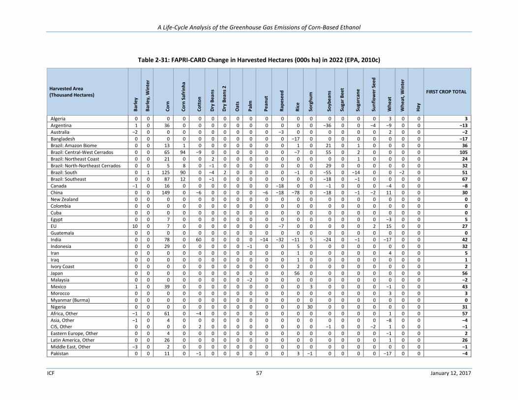
A Life-Cycle Analysis of the Greenhouse Gas Emissions of Corn-Based Ethanol
ICF 57 January 12, 2017
Table 2-31: FAPRI-CARD Change in Harvested Hectares (000s ha) in 2022 (EPA, 2010c)
Harvested Area (Thousand Hectares)
Bar
ley
Bar
ley,
Win
ter
Co
rn
Co
rn S
afri
nh
a
Co
tto
n
Dry
Be
ans
Dry
Be
ans
2
Oat
s
Pal
m
Pe
anu
t
Rap
ese
ed
Ric
e
Sorg
hu
m
Soyb
ean
s
Suga
r B
eet
Suga
rcan
e
Sun
flo
wer
Se
ed
Wh
eat
Wh
eat
, Win
ter
Hay
FIRST CROP TOTAL
Algeria 0 0 0 0 0 0 0 0 0 0 0 0 0 0 0 0 0 3 0 0 3
Argentina 1 0 36 0 0 0 0 0 0 0 0 0 0 −36 0 0 −4 −9 0 0 −13
Australia −2 0 0 0 0 0 0 0 0 0 −3 0 0 0 0 0 0 2 0 0 −2
Bangladesh 0 0 0 0 0 0 0 0 0 0 0 −17 0 0 0 0 0 0 0 0 −17
Brazil: Amazon Biome 0 0 13 1 0 0 0 0 0 0 0 1 0 21 0 1 0 0 0 0 36
Brazil: Central-West Cerrados 0 0 65 94 −9 0 0 0 0 0 0 −7 0 55 0 2 0 0 0 0 105
Brazil: Northeast Coast 0 0 21 0 0 2 0 0 0 0 0 0 0 0 0 1 0 0 0 0 24
Brazil: North-Northeast Cerrados 0 0 5 8 0 −1 0 0 0 0 0 0 0 29 0 0 0 0 0 0 32
Brazil: South 0 1 125 90 0 −4 2 0 0 0 0 −1 0 −55 0 −14 0 0 −2 0 51
Brazil: Southeast 0 0 87 12 0 −1 0 0 0 0 0 0 0 −18 0 −1 0 0 0 0 67
Canada −1 0 16 0 0 0 0 0 0 0 −18 0 0 −1 0 0 0 −4 0 0 −8
China 0 0 149 0 −6 0 0 0 0 −6 −18 −78 0 −18 0 −1 −2 11 0 0 30
New Zealand 0 0 0 0 0 0 0 0 0 0 0 0 0 0 0 0 0 0 0 0 0
Colombia 0 0 0 0 0 0 0 0 0 0 0 0 0 0 0 0 0 0 0 0 0
Cuba 0 0 0 0 0 0 0 0 0 0 0 0 0 0 0 0 0 0 0 0 0
Egypt 0 0 7 0 0 0 0 0 0 0 0 0 0 0 0 0 0 −3 0 0 5
EU 10 0 7 0 0 0 0 0 0 0 −7 0 0 0 0 0 2 15 0 0 27
Guatemala 0 0 0 0 0 0 0 0 0 0 0 0 0 0 0 0 0 0 0 0 0
India 0 0 78 0 60 0 0 0 0 −14 −32 −11 5 −24 0 −1 0 −17 0 0 42
Indonesia 0 0 29 0 0 0 0 0 −1 0 0 5 0 0 0 0 0 0 0 0 32
Iran 0 0 0 0 0 0 0 0 0 0 0 1 0 0 0 0 0 4 0 0 5
Iraq 0 0 0 0 0 0 0 0 0 0 0 1 0 0 0 0 0 0 0 0 1
Ivory Coast 0 0 0 0 0 0 0 0 0 0 0 2 0 0 0 0 0 0 0 0 2
Japan 0 0 0 0 0 0 0 0 0 0 0 56 0 0 0 0 0 0 0 0 56
Malaysia 0 0 0 0 0 0 0 0 −2 0 0 0 0 0 0 0 0 0 0 0 −2
Mexico 1 0 39 0 0 0 0 0 0 0 0 0 3 0 0 0 0 −1 0 0 43
Morocco 0 0 0 0 0 0 0 0 0 0 0 0 0 0 0 0 0 3 0 0 3
Myanmar (Burma) 0 0 0 0 0 0 0 0 0 0 0 0 0 0 0 0 0 0 0 0 0
Nigeria 0 0 0 0 0 0 0 0 0 0 0 0 30 0 0 0 0 0 0 0 31
Africa, Other −1 0 61 0 −4 0 0 0 0 0 0 0 0 0 0 0 0 1 0 0 57
Asia, Other −1 0 4 0 0 0 0 0 0 0 0 0 0 0 0 0 0 −8 0 0 −4 CIS, Other 0 0 0 0 2 0 0 0 0 0 0 0 0 −1 0 0 −2 1 0 0 −1
Eastern Europe, Other 0 0 4 0 0 0 0 0 0 0 0 0 0 0 0 0 0 −1 0 0 2
Latin America, Other 0 0 26 0 0 0 0 0 0 0 0 0 0 0 0 0 0 1 0 0 26
Middle East, Other −3 0 2 0 0 0 0 0 0 0 0 0 0 0 0 0 0 0 0 0 −1
Pakistan 0 0 11 0 −1 0 0 0 0 0 0 3 −1 0 0 0 0 −17 0 0 −4
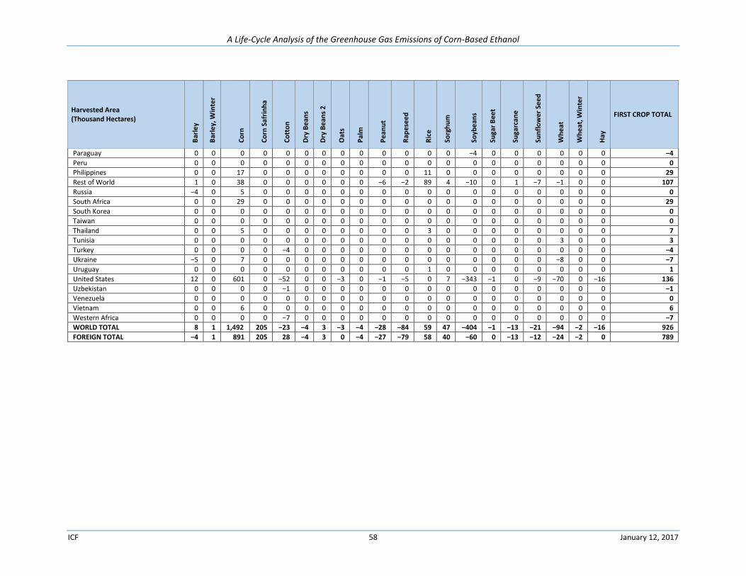
A Life-Cycle Analysis of the Greenhouse Gas Emissions of Corn-Based Ethanol
ICF 58 January 12, 2017
Harvested Area (Thousand Hectares)
Bar
ley
Bar
ley,
Win
ter
Co
rn
Co
rn S
afri
nh
a
Co
tto
n
Dry
Be
ans
Dry
Be
ans
2
Oat
s
Pal
m
Pe
anu
t
Rap
ese
ed
Ric
e
Sorg
hu
m
Soyb
ean
s
Suga
r B
eet
Suga
rcan
e
Sun
flo
wer
Se
ed
Wh
eat
Wh
eat
, Win
ter
Hay
FIRST CROP TOTAL
Paraguay 0 0 0 0 0 0 0 0 0 0 0 0 0 −4 0 0 0 0 0 0 −4
Peru 0 0 0 0 0 0 0 0 0 0 0 0 0 0 0 0 0 0 0 0 0
Philippines 0 0 17 0 0 0 0 0 0 0 0 11 0 0 0 0 0 0 0 0 29
Rest of World 1 0 38 0 0 0 0 0 0 −6 −2 89 4 −10 0 1 −7 −1 0 0 107
Russia −4 0 5 0 0 0 0 0 0 0 0 0 0 0 0 0 0 0 0 0 0
South Africa 0 0 29 0 0 0 0 0 0 0 0 0 0 0 0 0 0 0 0 0 29
South Korea 0 0 0 0 0 0 0 0 0 0 0 0 0 0 0 0 0 0 0 0 0
Taiwan 0 0 0 0 0 0 0 0 0 0 0 0 0 0 0 0 0 0 0 0 0
Thailand 0 0 5 0 0 0 0 0 0 0 0 3 0 0 0 0 0 0 0 0 7
Tunisia 0 0 0 0 0 0 0 0 0 0 0 0 0 0 0 0 0 3 0 0 3
Turkey 0 0 0 0 −4 0 0 0 0 0 0 0 0 0 0 0 0 0 0 0 −4
Ukraine −5 0 7 0 0 0 0 0 0 0 0 0 0 0 0 0 0 −8 0 0 −7
Uruguay 0 0 0 0 0 0 0 0 0 0 0 1 0 0 0 0 0 0 0 0 1
United States 12 0 601 0 −52 0 0 −3 0 −1 −5 0 7 −343 −1 0 −9 −70 0 −16 136
Uzbekistan 0 0 0 0 −1 0 0 0 0 0 0 0 0 0 0 0 0 0 0 0 −1
Venezuela 0 0 0 0 0 0 0 0 0 0 0 0 0 0 0 0 0 0 0 0 0
Vietnam 0 0 6 0 0 0 0 0 0 0 0 0 0 0 0 0 0 0 0 0 6
Western Africa 0 0 0 0 −7 0 0 0 0 0 0 0 0 0 0 0 0 0 0 0 −7
WORLD TOTAL 8 1 1,492 205 −23 −4 3 −3 −4 −28 −84 59 47 −404 −1 −13 −21 −94 −2 −16 926
FOREIGN TOTAL −4 1 891 205 28 −4 3 0 −4 −27 −79 58 40 −60 0 −13 −12 −24 −2 0 789
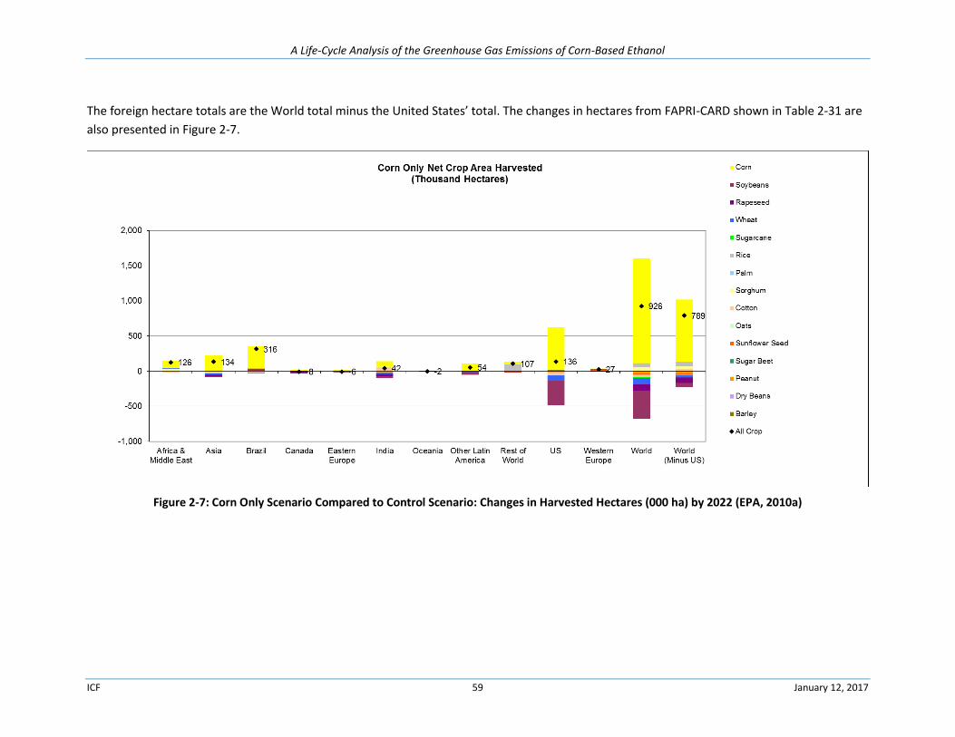
A Life-Cycle Analysis of the Greenhouse Gas Emissions of Corn-Based Ethanol
ICF 59 January 12, 2017
The foreign hectare totals are the World total minus the United States’ total. The changes in hectares from FAPRI-CARD shown in Table 2-31 are
also presented in Figure 2-7.
Figure 2-7: Corn Only Scenario Compared to Control Scenario: Changes in Harvested Hectares (000 ha) by 2022 (EPA, 2010a)
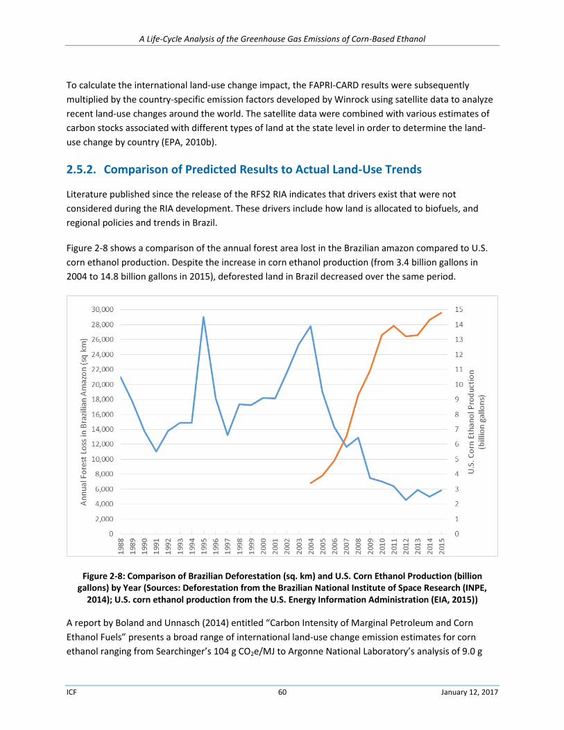
A Life-Cycle Analysis of the Greenhouse Gas Emissions of Corn-Based Ethanol
ICF 60 January 12, 2017
To calculate the international land-use change impact, the FAPRI-CARD results were subsequently
multiplied by the country-specific emission factors developed by Winrock using satellite data to analyze
recent land-use changes around the world. The satellite data were combined with various estimates of
carbon stocks associated with different types of land at the state level in order to determine the land-
use change by country (EPA, 2010b).
2.5.2. Comparison of Predicted Results to Actual Land-Use Trends
Literature published since the release of the RFS2 RIA indicates that drivers exist that were not
considered during the RIA development. These drivers include how land is allocated to biofuels, and
regional policies and trends in Brazil.
Figure 2-8 shows a comparison of the annual forest area lost in the Brazilian amazon compared to U.S.
corn ethanol production. Despite the increase in corn ethanol production (from 3.4 billion gallons in
2004 to 14.8 billion gallons in 2015), deforested land in Brazil decreased over the same period.
Figure 2-8: Comparison of Brazilian Deforestation (sq. km) and U.S. Corn Ethanol Production (billion gallons) by Year (Sources: Deforestation from the Brazilian National Institute of Space Research (INPE,
2014); U.S. corn ethanol production from the U.S. Energy Information Administration (EIA, 2015))
A report by Boland and Unnasch (2014) entitled “Carbon Intensity of Marginal Petroleum and Corn
Ethanol Fuels” presents a broad range of international land-use change emission estimates for corn
ethanol ranging from Searchinger’s 104 g CO2e/MJ to Argonne National Laboratory’s analysis of 9.0 g
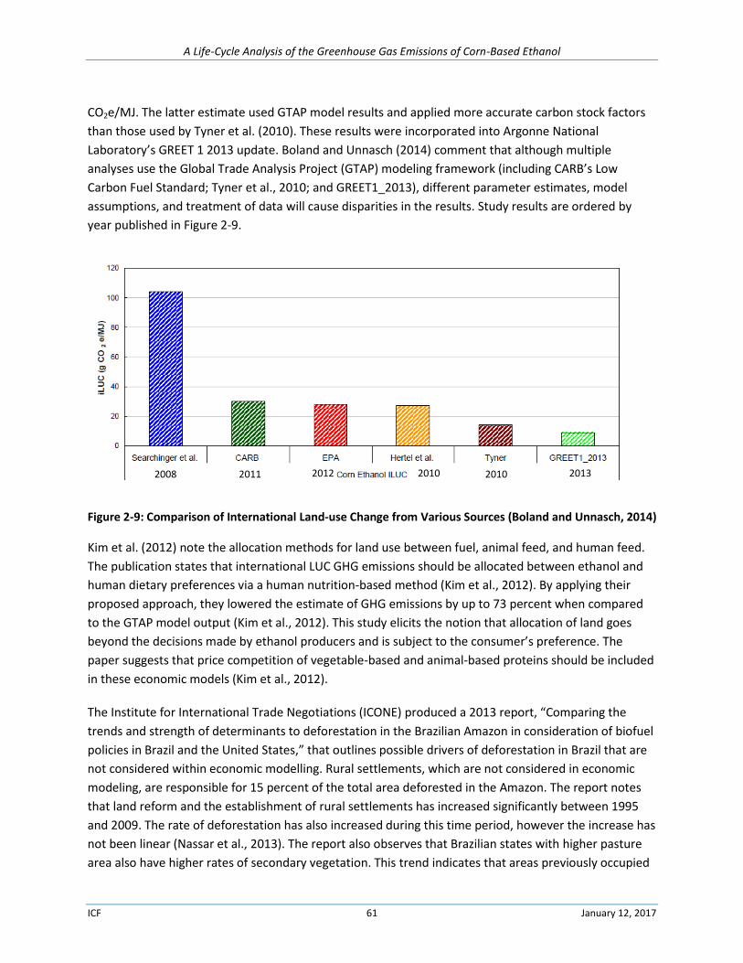
A Life-Cycle Analysis of the Greenhouse Gas Emissions of Corn-Based Ethanol
ICF 61 January 12, 2017
CO2e/MJ. The latter estimate used GTAP model results and applied more accurate carbon stock factors
than those used by Tyner et al. (2010). These results were incorporated into Argonne National
Laboratory’s GREET 1 2013 update. Boland and Unnasch (2014) comment that although multiple
analyses use the Global Trade Analysis Project (GTAP) modeling framework (including CARB’s Low
Carbon Fuel Standard; Tyner et al., 2010; and GREET1_2013), different parameter estimates, model
assumptions, and treatment of data will cause disparities in the results. Study results are ordered by
year published in Figure 2-9.
Figure 2-9: Comparison of International Land-use Change from Various Sources (Boland and Unnasch, 2014)
Kim et al. (2012) note the allocation methods for land use between fuel, animal feed, and human feed.
The publication states that international LUC GHG emissions should be allocated between ethanol and
human dietary preferences via a human nutrition-based method (Kim et al., 2012). By applying their
proposed approach, they lowered the estimate of GHG emissions by up to 73 percent when compared
to the GTAP model output (Kim et al., 2012). This study elicits the notion that allocation of land goes
beyond the decisions made by ethanol producers and is subject to the consumer’s preference. The
paper suggests that price competition of vegetable-based and animal-based proteins should be included
in these economic models (Kim et al., 2012).
The Institute for International Trade Negotiations (ICONE) produced a 2013 report, “Comparing the
trends and strength of determinants to deforestation in the Brazilian Amazon in consideration of biofuel
policies in Brazil and the United States,” that outlines possible drivers of deforestation in Brazil that are
not considered within economic modelling. Rural settlements, which are not considered in economic
modeling, are responsible for 15 percent of the total area deforested in the Amazon. The report notes
that land reform and the establishment of rural settlements has increased significantly between 1995
and 2009. The rate of deforestation has also increased during this time period, however the increase has
not been linear (Nassar et al., 2013). The report also observes that Brazilian states with higher pasture
area also have higher rates of secondary vegetation. This trend indicates that areas previously occupied
2008 2011 2012 2010 2010 2013
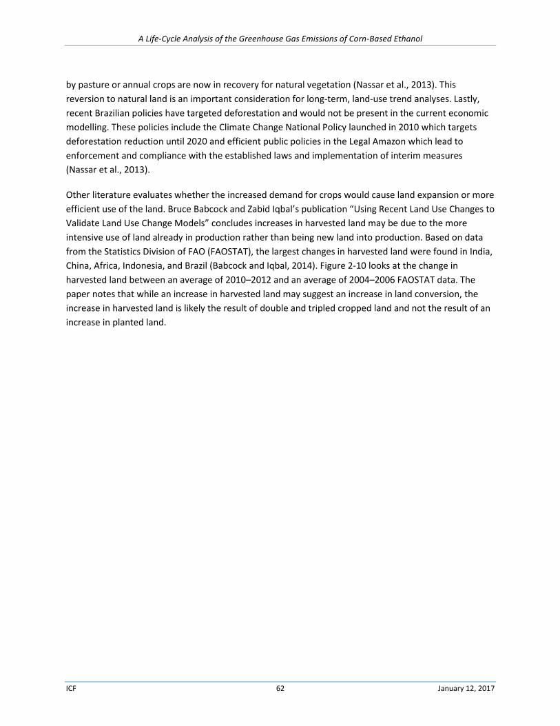
A Life-Cycle Analysis of the Greenhouse Gas Emissions of Corn-Based Ethanol
ICF 62 January 12, 2017
by pasture or annual crops are now in recovery for natural vegetation (Nassar et al., 2013). This
reversion to natural land is an important consideration for long-term, land-use trend analyses. Lastly,
recent Brazilian policies have targeted deforestation and would not be present in the current economic
modelling. These policies include the Climate Change National Policy launched in 2010 which targets
deforestation reduction until 2020 and efficient public policies in the Legal Amazon which lead to
enforcement and compliance with the established laws and implementation of interim measures
(Nassar et al., 2013).
Other literature evaluates whether the increased demand for crops would cause land expansion or more
efficient use of the land. Bruce Babcock and Zabid Iqbal’s publication “Using Recent Land Use Changes to
Validate Land Use Change Models” concludes increases in harvested land may be due to the more
intensive use of land already in production rather than being new land into production. Based on data
from the Statistics Division of FAO (FAOSTAT), the largest changes in harvested land were found in India,
China, Africa, Indonesia, and Brazil (Babcock and Iqbal, 2014). Figure 2-10 looks at the change in
harvested land between an average of 2010–2012 and an average of 2004–2006 FAOSTAT data. The
paper notes that while an increase in harvested land may suggest an increase in land conversion, the
increase in harvested land is likely the result of double and tripled cropped land and not the result of an
increase in planted land.
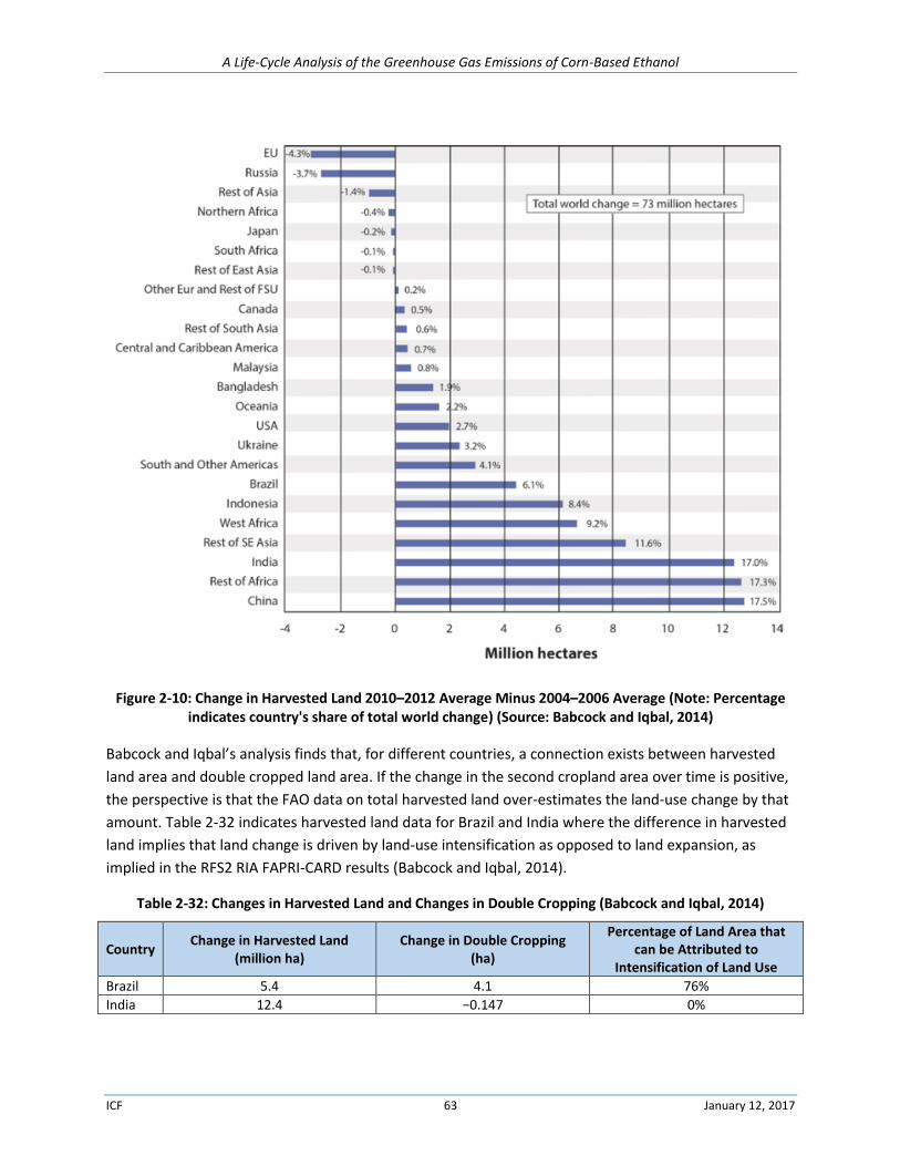
A Life-Cycle Analysis of the Greenhouse Gas Emissions of Corn-Based Ethanol
ICF 63 January 12, 2017
Figure 2-10: Change in Harvested Land 2010–2012 Average Minus 2004–2006 Average (Note: Percentage indicates country's share of total world change) (Source: Babcock and Iqbal, 2014)
Babcock and Iqbal’s analysis finds that, for different countries, a connection exists between harvested
land area and double cropped land area. If the change in the second cropland area over time is positive,
the perspective is that the FAO data on total harvested land over-estimates the land-use change by that
amount. Table 2-32 indicates harvested land data for Brazil and India where the difference in harvested
land implies that land change is driven by land-use intensification as opposed to land expansion, as
implied in the RFS2 RIA FAPRI-CARD results (Babcock and Iqbal, 2014).
Table 2-32: Changes in Harvested Land and Changes in Double Cropping (Babcock and Iqbal, 2014)
Country Change in Harvested Land
(million ha) Change in Double Cropping
(ha)
Percentage of Land Area that can be Attributed to
Intensification of Land Use
Brazil 5.4 4.1 76%
India 12.4 −0.147 0%
A Life-Cycle Analysis of the Greenhouse Gas Emissions of Corn-Based Ethanol
ICF 64 January 12, 2017
The intensification of land use in India shown in Table 2-32 is attributed to a 6 million hectare increase in
irrigated land. More irrigation allowed for a greater proportion of planted acres to be harvested. India
also increased its support prices and input subsidies in the mid-2000s, which increased the value of the
established cropland. The increased change in harvested land in sub-Saharan Africa is likely a better
measurement of the change in planted land given the proportion of African crop production that occurs
on small farms. Increased food production in the region matches the increase in the amount of land
planted. Lack of technology and capital signifies that double-cropping is not common. World-wide, the
extensive change (land expansion) was a net increase of 24 million hectares from 2004–2006 to 2010–
2012, while the aggregate intensive land-use change was 49.1 million hectares (Babcock and Iqbal,
2014). This difference led Babcock and Iqbal to conclude that the reliability of current models would be
increased if intensification of land use was considered.
2.5.2.1. Actual Land-Use Trends by Region
The FAPRI-CARD and GTAP models are the most widely used international models to predict land-use
changes associated with increased biofuel production. Both models allow crop yields to respond to an
increase in pricing, however they do not allow for adjustments in land-use intensity. Given the observed
trends presented above in Table 2-32, Babcock and Iqbal conclude that specific countries (e.g., Brazil)
and regions included within the EPA’s Renewable Fuel Standard Program Regulatory Impact Analysis
(RFS2 RIA) analysis have not followed the predicted trends from the FAPRI-CARD analysis (Babcock and
Iqbal, 2014).
Babcock and Iqbal looked at the intensive and extensive margin for each country/region in order to
determine how much of the change in land was attributable to land expansion or double cropping.
Intensive margin changes are those due to double cropping and a decrease in land that is planted but
not harvested. Extensive margin changes are those that show an increase in harvested land. Figure 2-11
below shows their analysis of FAOSTAT data between 2004–2006 to 2010–2012 for each country/region
indicating whether the change in harvested land area was intensive or extensive (Babcock and Iqbal,
2014).
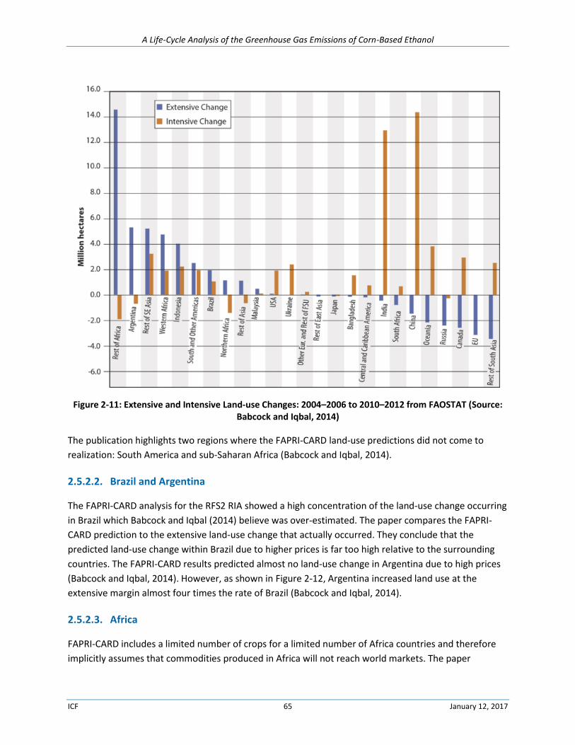
A Life-Cycle Analysis of the Greenhouse Gas Emissions of Corn-Based Ethanol
ICF 65 January 12, 2017
Figure 2-11: Extensive and Intensive Land-use Changes: 2004–2006 to 2010–2012 from FAOSTAT (Source: Babcock and Iqbal, 2014)
The publication highlights two regions where the FAPRI-CARD land-use predictions did not come to
realization: South America and sub-Saharan Africa (Babcock and Iqbal, 2014).
2.5.2.2. Brazil and Argentina
The FAPRI-CARD analysis for the RFS2 RIA showed a high concentration of the land-use change occurring
in Brazil which Babcock and Iqbal (2014) believe was over-estimated. The paper compares the FAPRI-
CARD prediction to the extensive land-use change that actually occurred. They conclude that the
predicted land-use change within Brazil due to higher prices is far too high relative to the surrounding
countries. The FAPRI-CARD results predicted almost no land-use change in Argentina due to high prices
(Babcock and Iqbal, 2014). However, as shown in Figure 2-12, Argentina increased land use at the
extensive margin almost four times the rate of Brazil (Babcock and Iqbal, 2014).
2.5.2.3. Africa
FAPRI-CARD includes a limited number of crops for a limited number of Africa countries and therefore
implicitly assumes that commodities produced in Africa will not reach world markets. The paper
A Life-Cycle Analysis of the Greenhouse Gas Emissions of Corn-Based Ethanol
ICF 66 January 12, 2017
comments that the large land-use changes shown in Figure 2-12 would have occurred regardless of high
commodity prices (Babcock and Iqbal, 2014). Based on this trend, the FAPRI-CARD results for the RFS2
RIA underestimated Africa’s connection to the world commodity market, and the impact that the
connectedness would have on extensive land-use change (Babcock and Iqbal, 2014).
2.5.3. Alternative to FAPRI-CARD Modelling
Given that the attributes and assumptions of the FAPRI-CARD analysis may not reflect actual land use
change trends, other models provide an alternative analysis to develop international land-use estimates.
FAPRI-CARD, as noted in Section 2.5.1, is a partial-equilibrium model that is multi-market and non-
spatial. Because the model is non-spatial, it does not distinguish between the sources and destinations
of trade between regions and countries (FAPRI, 2008). FAPRI did not develop an updated 2011 baseline
due to budget constraints, causing this data output to be antiquated.
GTAP is a computable equilibrium model with perfect competition and links production and
consumption by region. The GTAP-BIO model is specifically tailored to estimate the land use impact of
an exogenous policy shock. The GTAP-BIO database has been updated based on trends in land-use
patterns and updated data are available. In the EPA RIA analysis, geospatial data was used to distinguish
which types of land were converted and reverted while GTAP’s output includes this modeled data.
GTAP allows three land types to be used for biofuel production: forest, grassland, and cropland-pasture
land. Crop-pasture land is agricultural land that has been converted to agriculture dominated by the
production of biofuel feedstocks. GTAP results are available for two pertinent biofuel production
scenarios. Both scenarios reflect a shock of 11.59 billion gallons of increased demand for corn as a
feedstock commodity. Scenario Case A was modeled in 2011 and Case H was modelled in 2013 (Argonne
National Laboratory, 2014). The production scenarios are shown below in Table 2-33 and were taken
from Argonne National Laboratory’s Carbon Calculator for Land Use Change from Biofuels Production
(CCLUB) model.
Table 2-33: GTAP Modeling Scenarios (Argonne National Laboratory, 2014)
Case18
Case Description Gallons Source
A An increase in corn ethanol production from its 2004 level (3.41 billion gallons [BG]) to 15 BG
11.59 Taheripour et al., 2011
H An increase in corn ethanol production from its 2004 level (3.41 BG) to 15 BG with GTAP recalibrated land transformation parameters
11.59 Taheripour and Tyner, 2013
Although Case A and H model the same production volume, there were key aspects within the GTAP
model run that cause different results.
18 Note: Case lettering is referred to within the cited publications.
A Life-Cycle Analysis of the Greenhouse Gas Emissions of Corn-Based Ethanol
ICF 67 January 12, 2017
Land Transformation: Land transformation elasticity reflects the ease of land transition from one
state to another. A low value indicates limited land transitions. In 2011, GTAP included only one land
transformation elasticity for the world. Taheripour and Tyner (2013) updated the land
transformation data to develop region-specific elasticities using two United Nations Food and
Agriculture Organization land-cover datasets. The updates allowed for determination of changes in
agricultural land area and the characterization of changes in harvested area for crop types. Based on
this change, Taheripour and Tyner (2013) found that that the United States moved a sizeable
amount of agricultural land to produce corn and oilseed crops without significant expansion in
overall agricultural land (Argonne National Laboratory, 2014).
Treatment of Conversion Costs: In 2011, converting pasture and forest to cropland cost the same
amount. In 2013, GTAP was adjusted to reflect the greater cost of converting of forest to cropland
compared to converting pasture to cropland. In the updated dataset, it is more costly to convert
forest to cropland than in the prior model version.
Taheripour and Tyner (2013) used observed land-use trends as a guide for the most recent update of
GTAP. This methodology was used to reconcile the differences between modeled predictions and the
observed trends. They specifically address how land-use changes responded to changes in global
commodity pricing.
The raw GTAP data is grouped by land-use type (forest, grassland, cropland pasture, and cropland). Each
country/region contains the hectares converted for each of the 18 Agro-ecological Zones (AEZ). A
summary table of the GTAP total hectares by region for Scenario A is shown below in Table 2-34 and
Scenario H is shown in Table 2-35 (Argonne National Laboratory, 2014).
The GTAP 2011 data (Scenario A) shows an increase in international (excluding U.S.) Forest and Cropland
acres while there is a decrease in Grassland and Cropland-Grassland acres. The international change in
hectares for GTAP 2013 output shows similar trends for Cropland, Grassland, and Cropland-Grassland
hectares although the change for each category is consistently smaller. For the change in Forest
hectares, the GTAP 2013 output shows a decrease in area change—a difference of 123,249 hectares.
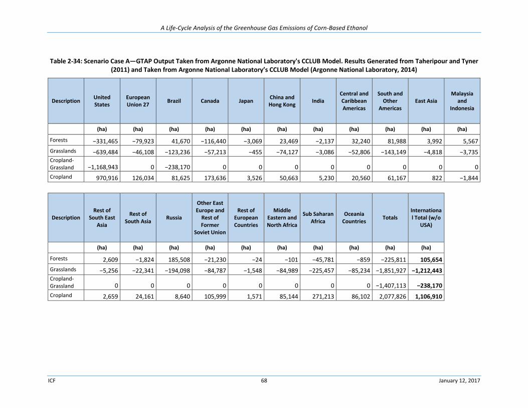
A Life-Cycle Analysis of the Greenhouse Gas Emissions of Corn-Based Ethanol
ICF 68 January 12, 2017
Table 2-34: Scenario Case A—GTAP Output Taken from Argonne National Laboratory's CCLUB Model. Results Generated from Taheripour and Tyner (2011) and Taken from Argonne National Laboratory’s CCLUB Model (Argonne National Laboratory, 2014)
Description United States
European Union 27
Brazil Canada Japan China and Hong Kong
India Central and Caribbean Americas
South and Other
Americas East Asia
Malaysia and
Indonesia
(ha) (ha) (ha) (ha) (ha) (ha) (ha) (ha) (ha) (ha) (ha)
Forests −331,465 −79,923 41,670 −116,440 −3,069 23,469 −2,137 32,240 81,988 3,992 5,567
Grasslands −639,484 −46,108 −123,236 −57,213 −455 −74,127 −3,086 −52,806 −143,149 −4,818 −3,735
Cropland-Grassland −1,168,943 0 −238,170 0 0 0 0 0 0 0 0
Cropland 970,916 126,034 81,625 173,636 3,526 50,663 5,230 20,560 61,167 822 −1,844
Description Rest of
South East Asia
Rest of South Asia
Russia
Other East Europe and
Rest of Former
Soviet Union
Rest of European Countries
Middle Eastern and North Africa
Sub Saharan Africa
Oceania Countries
Totals International Total (w/o
USA)
(ha) (ha) (ha) (ha) (ha) (ha) (ha) (ha) (ha) (ha)
Forests 2,609 −1,824 185,508 −21,230 −24 −101 −45,781 −859 −225,811 105,654
Grasslands −5,256 −22,341 −194,098 −84,787 −1,548 −84,989 −225,457 −85,234 −1,851,927 −1,212,443
Cropland-Grassland 0 0 0 0 0 0 0 0 −1,407,113 −238,170
Cropland 2,659 24,161 8,640 105,999 1,571 85,144 271,213 86,102 2,077,826 1,106,910
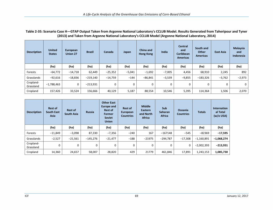
A Life-Cycle Analysis of the Greenhouse Gas Emissions of Corn-Based Ethanol
ICF 69 January 12, 2017
Table 2-35: Scenario Case H—GTAP Output Taken from Argonne National Laboratory's CCLUB Model. Results Generated from Taheripour and Tyner (2013) and Taken from Argonne National Laboratory’s CCLUB Model (Argonne National Laboratory, 2014)
Description United States
European Union 27
Brazil Canada Japan China and Hong Kong
India
Central and
Caribbean Americas
South and Other
Americas East Asia
Malaysia and
Indonesia
(ha) (ha) (ha) (ha) (ha) (ha) (ha) (ha) (ha) (ha) (ha)
Forests −64,772 −14,718 62,449 −25,352 −5,041 −1,692 −7,005 4,456 68,910 2,245 892
Grasslands −92,616 −18,836 −219,140 −14,759 −144 −86,841 −3,539 −9,855 −183,326 −3,762 −2,973
Cropland-Grassland
−1,788,463 0 −213,931 0 0 0 0 0 0 0 0
Cropland 157,426 33,524 156,666 40,129 5,187 88,554 10,546 5,395 114,364 1,506 2,070
Description Rest of
South East Asia
Rest of South Asia
Russia
Other East Europe and
Rest of Former Soviet Union
Rest of European Countries
Middle Eastern
and North Africa
Sub Saharan
Africa
Oceania Countries
Totals Internation
al Total (w/o USA)
(ha) (ha) (ha) (ha) (ha) (ha) (ha) (ha) (ha) (ha)
Forests −11,849 −3,098 87,330 −7,356 −240 167 −167148 −545 −82369 −17,595
Grasslands −2,527 −21,561 −145,276 −21,477 −188 −21975 −294,787 −17,308 −1,160,891 −1,068,274
Cropland-Grassland
0 0 0 0 0 0 0 0 −2,002,393 −213,931
Cropland 14,360 24,657 58,007 28,820 429 21779 461,846 17,891 1,243,153 1,085,730
A Life-Cycle Analysis of the Greenhouse Gas Emissions of Corn-Based Ethanol
ICF 70 January 12, 2017
2.5.4. References: International Land-Use Change
Babcock, B.A. and Iqbal, Z., 2014. “Using Recent Land Use Changes to Validate Land Use Change Models”. Staff Report 14-SR 109. Center for Agricultural and Rural Development: Iowa State University. http://www.card.iastate.edu/publications/dbs/pdffiles/14sr109.pdf
Boland. S. and Unnasch. S., 2014. Carbon Intensity of Marginal Petroleum and Corn Ethanol Fuels. Life Cycle Associates Report LCA.6075.83.2014, Prepared for Renewable Fuels Association.
Used data cited within Boland and Unnsach but originally cited in:
Dunn, J., Mueller, S., Kwon, H.Y. and Wang, M.Q., 2013. Land-Use Change and Greenhouse Gas Emissions from Corn and Cellulosic Ethanol. Biotechnology for Biofuels 2013, (6) pp. 51
Hertel, T.W., Golub, A.A., Jones, A.D., O’Hare, M., Plevin, R.J., & Kammen, D.M., 2010. Global land use and greenhouse gas emissions impacts of U.S. maize ethanol: Estimating market-mediated responses. Bioscience, 60, pp. 223-231.
Searchinger, T., Heimlich, R., Houghton, R.A., Dong, F., Elobeid, A., Fabiosa, J., et al., 2008. Use of U.S. croplands for biofuels increases greenhouse gases through emissions from land-use change. Science, 319 (5867), pp. 1238-1240
Tyner, W. E. Taheripour, F., Zhuang, Q., Birur, B., 2010. Land Use Changes and Consequent CO2 Emissions Due to US Corn Ethanol Production: A Comprehensive Analysis, Department of Agricultural Economics, Purdue University, Report to Argonne National Laboratory.
Dunn JB, Mueller S, Qin Z, Wang MQ (2014) Carbon Calculator for Land Use Change from Biofuels Production (CCLUB 2015). Argonne National Laboratory (ANL).
EIA, 2015. U.S. Energy Information Administration/ Monthly Energy Review. Table 10.3 Fuel Ethanol Overview. December 2015. http://www.eia.gov/totalenergy/data/monthly/#renewable
EPA, 2010c. Memorandum to Docket. SUBJECT: Fapri-Card Lifecycle GHG (Greenhouse Gases) Analysis Results (January 29, 2010) from Docket. Regulations.gov, ID: EPA-HQ-OAR-2005-0161-3153. Posted March 26, 2010. http://www.regulations.gov/#!documentDetail;D=EPA-HQ-OAR-2005-0161-3153
EPA, 2010a. Renewable Fuel Standard (RFS2) Final Regulatory Impact Analysis. EPA-420-R-10-006. Available: http://www3.epa.gov/otaq/renewablefuels/420r10006.pdf
FAO, 2009. FAOStat Production (Crops). Retrieved from FAOStat: http://faostat.fao.org/site/567/DesktopDefault.aspx?PageID=567#ancor
FAPRI (2008) Biofuels: Impacts of Selected Farm Bill Provisions and Other Biofuel Policy Options. Available online at: http://www.fapri.missouri.edu/outreach/publications/2008/FAPRI_MU_Report_06_08.pdf
Kim, S.K., Dale, B.E. and Ong, R.G., 2012. An alternative approach to indirect land use change: Allocating greenhouse gas effects among different uses of land. Biomass and Bioenergy (46). 447-42.
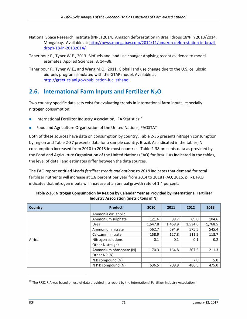
A Life-Cycle Analysis of the Greenhouse Gas Emissions of Corn-Based Ethanol
ICF 71 January 12, 2017
National Space Research Institute (INPE) 2014. Amazon deforestation in Brazil drops 18% in 2013/2014. Mongabay. Available at: http://news.mongabay.com/2014/11/amazon-deforestation-in-brazil-drops-18-in-20132014/
Taheripour F., Tyner W.E., 2013. Biofuels and land use change: Applying recent evidence to model estimates. Applied Sciences, 3, 14–38.
Taheripour F., Tyner W.E., and Wang M.Q., 2011. Global land use change due to the U.S. cellulosic biofuels program simulated with the GTAP model. Available at http://greet.es.anl.gov/publication-luc_ethanol.
2.6. International Farm Inputs and Fertilizer N2O
Two country-specific data sets exist for evaluating trends in international farm inputs, especially
nitrogen consumption:
International Fertilizer Industry Association, IFA Statistics19
Food and Agriculture Organization of the United Nations, FAOSTAT
Both of these sources have data on consumption by country. Table 2-36 presents nitrogen consumption
by region and Table 2-37 presents data for a sample country, Brazil. As indicated in the tables, N
consumption increased from 2010 to 2013 in most countries. Table 2-38 presents data as provided by
the Food and Agriculture Organization of the United Nations (FAO) for Brazil. As indicated in the tables,
the level of detail and estimates differ between the data sources.
The FAO report entitled World fertilizer trends and outlook to 2018 indicates that demand for total
fertilizer nutrients will increase at 1.8 percent per year from 2014 to 2018 (FAO, 2015, p. ix). FAO
indicates that nitrogen inputs will increase at an annual growth rate of 1.4 percent.
Table 2-36: Nitrogen Consumption by Region by Calendar Year as Provided by International Fertilizer Industry Association (metric tons of N)
Country Product 2010 2011 2012 2013
Africa
Ammonia dir. applic.
Ammonium sulphate 121.6 99.7 69.0 104.6
Urea 1,647.8 1,468.9 1,534.6 1,768.5
Ammonium nitrate 562.7 594.9 575.5 545.4
Calc.amm. nitrate 158.9 127.8 111.5 118.7
Nitrogen solutions 0.1 0.1 0.1 0.2
Other N straight
Ammonium phosphate (N) 170.3 164.8 207.5 211.3
Other NP (N)
N K compound (N) 7.0 5.0
N P K compound (N) 636.5 709.9 486.5 475.0
19 The RFS2 RIA was based on use of data provided in a report by the International Fertilizer Industry Association.
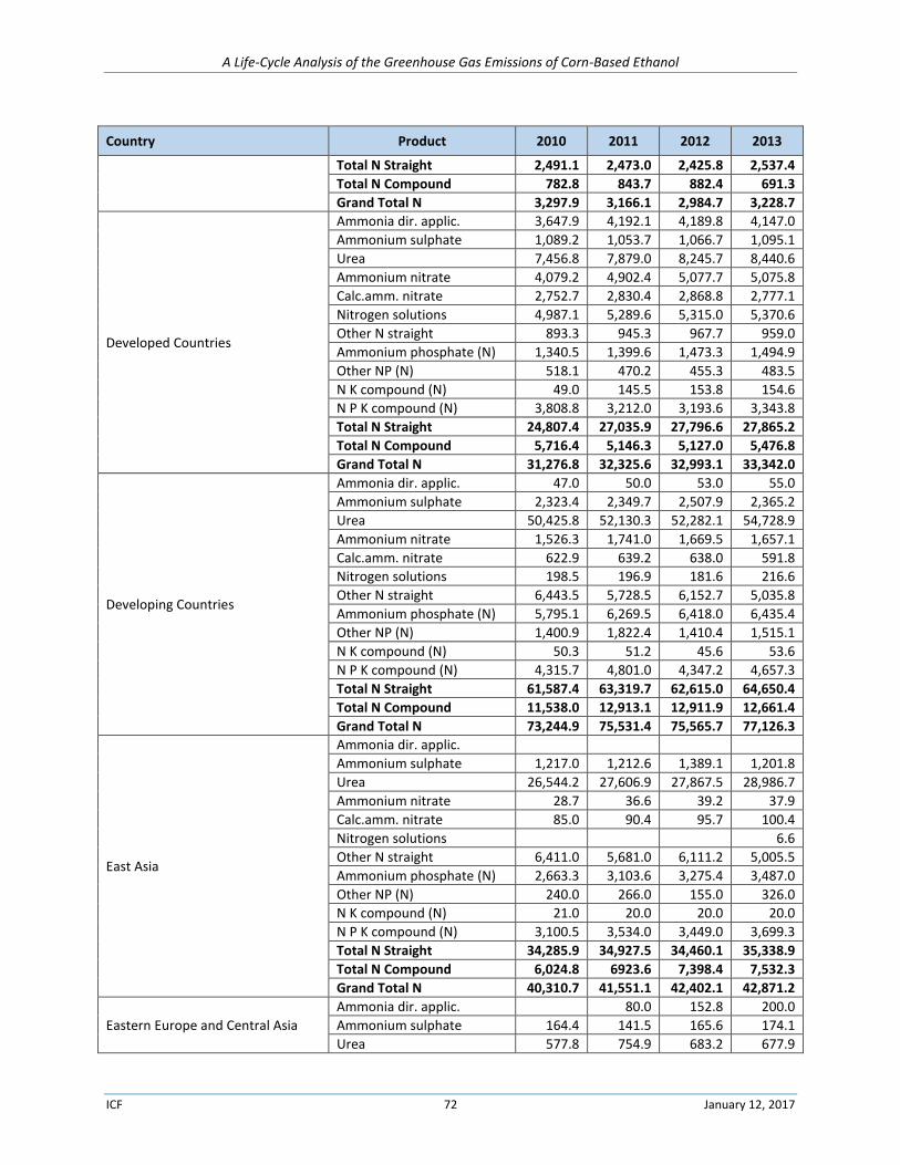
A Life-Cycle Analysis of the Greenhouse Gas Emissions of Corn-Based Ethanol
ICF 72 January 12, 2017
Country Product 2010 2011 2012 2013
Total N Straight 2,491.1 2,473.0 2,425.8 2,537.4
Total N Compound 782.8 843.7 882.4 691.3
Grand Total N 3,297.9 3,166.1 2,984.7 3,228.7
Developed Countries
Ammonia dir. applic. 3,647.9 4,192.1 4,189.8 4,147.0
Ammonium sulphate 1,089.2 1,053.7 1,066.7 1,095.1
Urea 7,456.8 7,879.0 8,245.7 8,440.6
Ammonium nitrate 4,079.2 4,902.4 5,077.7 5,075.8
Calc.amm. nitrate 2,752.7 2,830.4 2,868.8 2,777.1
Nitrogen solutions 4,987.1 5,289.6 5,315.0 5,370.6
Other N straight 893.3 945.3 967.7 959.0
Ammonium phosphate (N) 1,340.5 1,399.6 1,473.3 1,494.9
Other NP (N) 518.1 470.2 455.3 483.5
N K compound (N) 49.0 145.5 153.8 154.6
N P K compound (N) 3,808.8 3,212.0 3,193.6 3,343.8
Total N Straight 24,807.4 27,035.9 27,796.6 27,865.2
Total N Compound 5,716.4 5,146.3 5,127.0 5,476.8
Grand Total N 31,276.8 32,325.6 32,993.1 33,342.0
Developing Countries
Ammonia dir. applic. 47.0 50.0 53.0 55.0
Ammonium sulphate 2,323.4 2,349.7 2,507.9 2,365.2
Urea 50,425.8 52,130.3 52,282.1 54,728.9
Ammonium nitrate 1,526.3 1,741.0 1,669.5 1,657.1
Calc.amm. nitrate 622.9 639.2 638.0 591.8
Nitrogen solutions 198.5 196.9 181.6 216.6
Other N straight 6,443.5 5,728.5 6,152.7 5,035.8
Ammonium phosphate (N) 5,795.1 6,269.5 6,418.0 6,435.4
Other NP (N) 1,400.9 1,822.4 1,410.4 1,515.1
N K compound (N) 50.3 51.2 45.6 53.6
N P K compound (N) 4,315.7 4,801.0 4,347.2 4,657.3
Total N Straight 61,587.4 63,319.7 62,615.0 64,650.4
Total N Compound 11,538.0 12,913.1 12,911.9 12,661.4
Grand Total N 73,244.9 75,531.4 75,565.7 77,126.3
East Asia
Ammonia dir. applic.
Ammonium sulphate 1,217.0 1,212.6 1,389.1 1,201.8
Urea 26,544.2 27,606.9 27,867.5 28,986.7
Ammonium nitrate 28.7 36.6 39.2 37.9
Calc.amm. nitrate 85.0 90.4 95.7 100.4
Nitrogen solutions 6.6
Other N straight 6,411.0 5,681.0 6,111.2 5,005.5
Ammonium phosphate (N) 2,663.3 3,103.6 3,275.4 3,487.0
Other NP (N) 240.0 266.0 155.0 326.0
N K compound (N) 21.0 20.0 20.0 20.0
N P K compound (N) 3,100.5 3,534.0 3,449.0 3,699.3
Total N Straight 34,285.9 34,927.5 34,460.1 35,338.9
Total N Compound 6,024.8 6923.6 7,398.4 7,532.3
Grand Total N 40,310.7 41,551.1 42,402.1 42,871.2
Eastern Europe and Central Asia
Ammonia dir. applic. 80.0 152.8 200.0
Ammonium sulphate 164.4 141.5 165.6 174.1
Urea 577.8 754.9 683.2 677.9
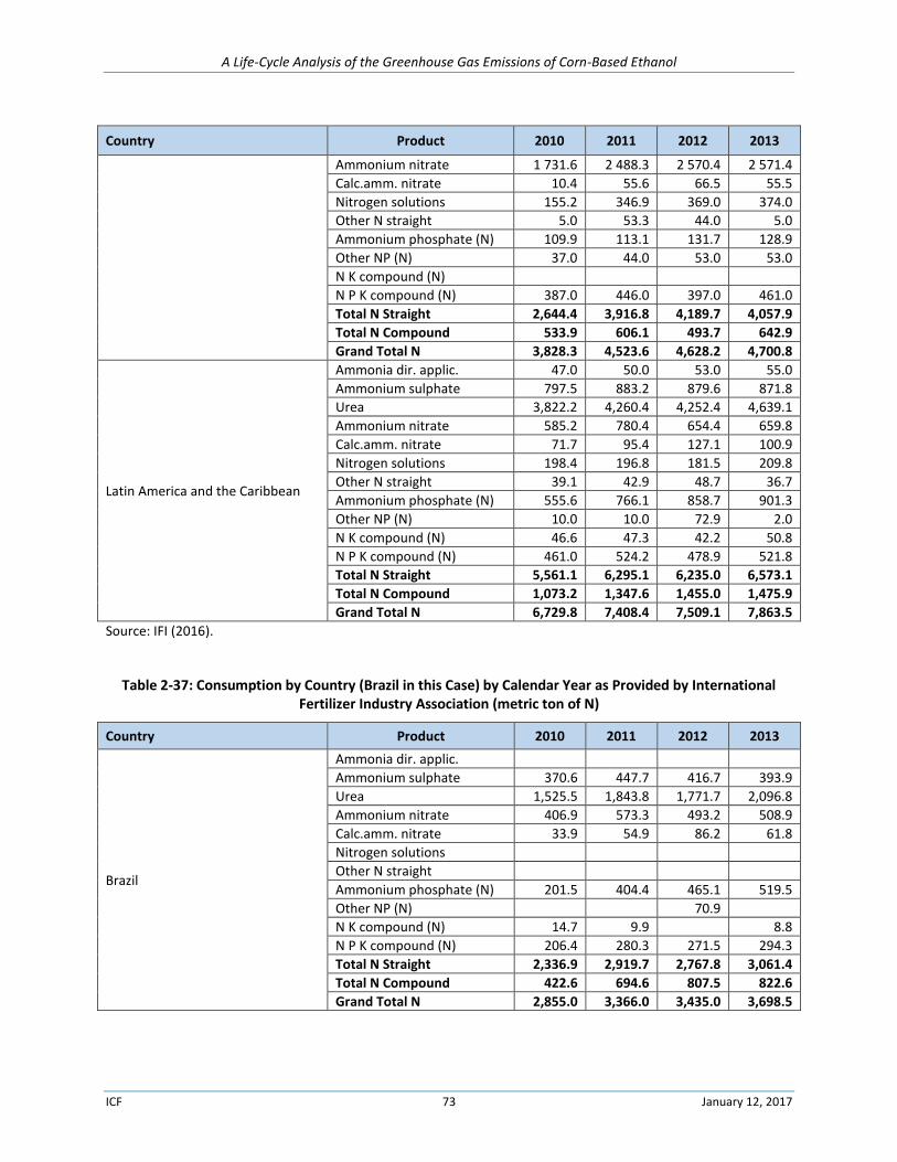
A Life-Cycle Analysis of the Greenhouse Gas Emissions of Corn-Based Ethanol
ICF 73 January 12, 2017
Country Product 2010 2011 2012 2013
Ammonium nitrate 1 731.6 2 488.3 2 570.4 2 571.4
Calc.amm. nitrate 10.4 55.6 66.5 55.5
Nitrogen solutions 155.2 346.9 369.0 374.0
Other N straight 5.0 53.3 44.0 5.0
Ammonium phosphate (N) 109.9 113.1 131.7 128.9
Other NP (N) 37.0 44.0 53.0 53.0
N K compound (N)
N P K compound (N) 387.0 446.0 397.0 461.0
Total N Straight 2,644.4 3,916.8 4,189.7 4,057.9
Total N Compound 533.9 606.1 493.7 642.9
Grand Total N 3,828.3 4,523.6 4,628.2 4,700.8
Latin America and the Caribbean
Ammonia dir. applic. 47.0 50.0 53.0 55.0
Ammonium sulphate 797.5 883.2 879.6 871.8
Urea 3,822.2 4,260.4 4,252.4 4,639.1
Ammonium nitrate 585.2 780.4 654.4 659.8
Calc.amm. nitrate 71.7 95.4 127.1 100.9
Nitrogen solutions 198.4 196.8 181.5 209.8
Other N straight 39.1 42.9 48.7 36.7
Ammonium phosphate (N) 555.6 766.1 858.7 901.3
Other NP (N) 10.0 10.0 72.9 2.0
N K compound (N) 46.6 47.3 42.2 50.8
N P K compound (N) 461.0 524.2 478.9 521.8
Total N Straight 5,561.1 6,295.1 6,235.0 6,573.1
Total N Compound 1,073.2 1,347.6 1,455.0 1,475.9
Grand Total N 6,729.8 7,408.4 7,509.1 7,863.5
Source: IFI (2016).
Table 2-37: Consumption by Country (Brazil in this Case) by Calendar Year as Provided by International Fertilizer Industry Association (metric ton of N)
Country Product 2010 2011 2012 2013
Brazil
Ammonia dir. applic.
Ammonium sulphate 370.6 447.7 416.7 393.9
Urea 1,525.5 1,843.8 1,771.7 2,096.8
Ammonium nitrate 406.9 573.3 493.2 508.9
Calc.amm. nitrate 33.9 54.9 86.2 61.8
Nitrogen solutions
Other N straight
Ammonium phosphate (N) 201.5 404.4 465.1 519.5
Other NP (N) 70.9
N K compound (N) 14.7 9.9 8.8
N P K compound (N) 206.4 280.3 271.5 294.3
Total N Straight 2,336.9 2,919.7 2,767.8 3,061.4
Total N Compound 422.6 694.6 807.5 822.6
Grand Total N 2,855.0 3,366.0 3,435.0 3,698.5
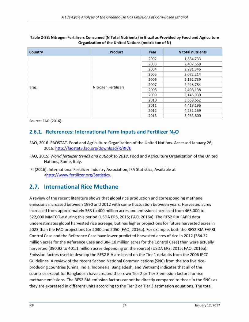
A Life-Cycle Analysis of the Greenhouse Gas Emissions of Corn-Based Ethanol
ICF 74 January 12, 2017
Table 2-38: Nitrogen Fertilizers Consumed (N Total Nutrients) in Brazil as Provided by Food and Agriculture Organization of the United Nations (metric ton of N)
Country Product Year N total nutrients
Brazil Nitrogen Fertilizers
2002 1,834,733
2003 2,407,558
2004 2,281,346
2005 2,072,214
2006 2,192,739
2007 2,948,784
2008 2,498,138
2009 3,145,930
2010 3,668,652
2011 4,418,196
2012 4,251,169
2013 3,953,800
Source: FAO (2016).
2.6.1. References: International Farm Inputs and Fertilizer N2O
FAO, 2016. FAOSTAT. Food and Agriculture Organization of the United Nations. Accessed January 26, 2016. http://faostat3.fao.org/download/R/RF/E
FAO, 2015. World fertilizer trends and outlook to 2018, Food and Agriculture Organization of the United Nations, Rome, Italy.
IFI (2016). International Fertilizer Industry Association, IFA Statistics, Available at <http://www.fertilizer.org/Statistics.
2.7. International Rice Methane
A review of the recent literature shows that global rice production and corresponding methane
emissions increased between 1990 and 2012 with some fluctuation between years. Harvested acres
increased from approximately 363 to 400 million acres and emissions increased from 465,000 to
522,000 MMTCO2e during this period (USDA ERS, 2015; FAO, 2016a). The RFS2 RIA FAPRI data
underestimates global harvested rice acreage, but has higher projections for future harvested acres in
2023 than the FAO projections for 2030 and 2050 (FAO, 2016a). For example, both the RFS2 RIA FAPRI
Control Case and the Reference Case have lower predicted harvested acres of rice in 2012 (384.32
million acres for the Reference Case and 384.10 million acres for the Control Case) than were actually
harvested (390.92 to 401.1 million acres depending on the source) (USDA ERS, 2015; FAO, 2016a).
Emission factors used to develop the RFS2 RIA are based on the Tier 1 defaults from the 2006 IPCC
Guidelines. A review of the recent Second National Communications (SNC) from the top five rice-
producing countries (China, India, Indonesia, Bangladesh, and Vietnam) indicates that all of the
countries except for Bangladesh have created their own Tier 2 or Tier 3 emission factors for rice
methane emissions. The RFS2 RIA emission factors cannot be directly compared to those in the SNCs as
they are expressed in different units according to the Tier 2 or Tier 3 estimation equations. The total
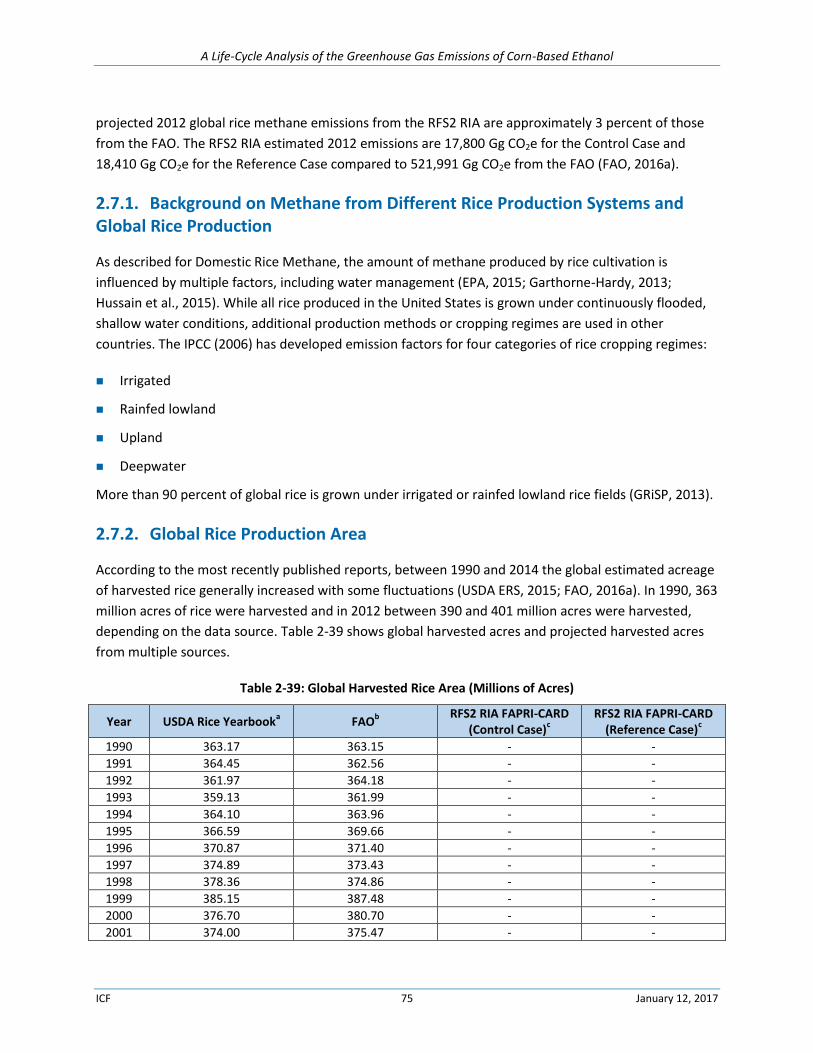
A Life-Cycle Analysis of the Greenhouse Gas Emissions of Corn-Based Ethanol
ICF 75 January 12, 2017
projected 2012 global rice methane emissions from the RFS2 RIA are approximately 3 percent of those
from the FAO. The RFS2 RIA estimated 2012 emissions are 17,800 Gg CO2e for the Control Case and
18,410 Gg CO2e for the Reference Case compared to 521,991 Gg CO2e from the FAO (FAO, 2016a).
2.7.1. Background on Methane from Different Rice Production Systems and Global Rice Production
As described for Domestic Rice Methane, the amount of methane produced by rice cultivation is
influenced by multiple factors, including water management (EPA, 2015; Garthorne-Hardy, 2013;
Hussain et al., 2015). While all rice produced in the United States is grown under continuously flooded,
shallow water conditions, additional production methods or cropping regimes are used in other
countries. The IPCC (2006) has developed emission factors for four categories of rice cropping regimes:
Irrigated
Rainfed lowland
Upland
Deepwater
More than 90 percent of global rice is grown under irrigated or rainfed lowland rice fields (GRiSP, 2013).
2.7.2. Global Rice Production Area
According to the most recently published reports, between 1990 and 2014 the global estimated acreage
of harvested rice generally increased with some fluctuations (USDA ERS, 2015; FAO, 2016a). In 1990, 363
million acres of rice were harvested and in 2012 between 390 and 401 million acres were harvested,
depending on the data source. Table 2-39 shows global harvested acres and projected harvested acres
from multiple sources.
Table 2-39: Global Harvested Rice Area (Millions of Acres)
Year USDA Rice Yearbooka FAO
b
RFS2 RIA FAPRI-CARD (Control Case)
c RFS2 RIA FAPRI-CARD
(Reference Case)c
1990 363.17 363.15 - -
1991 364.45 362.56 - -
1992 361.97 364.18 - -
1993 359.13 361.99 - -
1994 364.10 363.96 - -
1995 366.59 369.66 - -
1996 370.87 371.40 - -
1997 374.89 373.43 - -
1998 378.36 374.86 - -
1999 385.15 387.48 - -
2000 376.70 380.70 - -
2001 374.00 375.47 - -
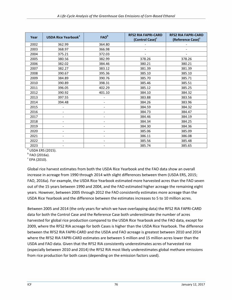
A Life-Cycle Analysis of the Greenhouse Gas Emissions of Corn-Based Ethanol
ICF 76 January 12, 2017
Year USDA Rice Yearbooka FAO
b
RFS2 RIA FAPRI-CARD (Control Case)
c RFS2 RIA FAPRI-CARD
(Reference Case)c
2002 362.99 364.80 - -
2003 368.97 366.98 - -
2004 375.21 372.03 - -
2005 380.56 382.99 378.26 378.26
2006 382.02 384.46 380.21 380.21
2007 382.27 383.12 381.39 381.39
2008 390.67 395.36 385.10 385.10
2009 384.89 390.76 385.70 385.71
2010 390.89 398.31 385.46 385.51
2011 396.05 402.29 385.12 385.25
2012 390.92 401.10 384.10 384.32
2013 397.55 - 383.88 383.56
2014 394.48 - 384.26 383.96
2015 - - 384.59 384.32
2016 - - 384.73 384.47
2017 - - 384.46 384.19
2018 - - 384.34 384.25
2019 - - 384.30 384.36
2020 - - 385.06 385.09
2021 - - 386.11 386.08
2022 - - 385.56 385.48
2023 - - 385.74 385.65 a USDA ERS (2015).
b FAO (2016a).
c EPA (2010).
Global rice harvest estimates from both the USDA Rice Yearbook and the FAO data show an overall
increase in acreage from 1990 through 2014 with slight differences between them (USDA ERS, 2015;
FAO, 2016a). For example, the USDA Rice Yearbook estimated more harvested acres than the FAO seven
out of the 15 years between 1990 and 2004, and the FAO estimated higher acreage the remaining eight
years. However, between 2005 through 2012 the FAO consistently estimates more acreage than the
USDA Rice Yearbook and the difference between the estimates increases to 5 to 10 million acres.
Between 2005 and 2014 (the only years for which we have overlapping data) the RFS2 RIA FAPRI-CARD
data for both the Control Case and the Reference Case both underestimate the number of acres
harvested for global rice production compared to the USDA Rice Yearbook and the FAO data, except for
2009, where the RFS2 RIA acreage for both Cases is higher than the USDA Rice Yearbook. The difference
between the RFS2 RIA FAPRI-CARD and the USDA and FAO acreage is greatest between 2010 and 2014
where the RFS2 RIA FAPRI-CARD estimates are between 5 million and 15 million acres lower than the
USDA and FAO data. Given that the RFS2 RIA consistently underestimates acres of harvested rice
(especially between 2010 and 2014) the RFS2 RIA most likely underestimates global methane emissions
from rice production for both cases (depending on the emission factors used).
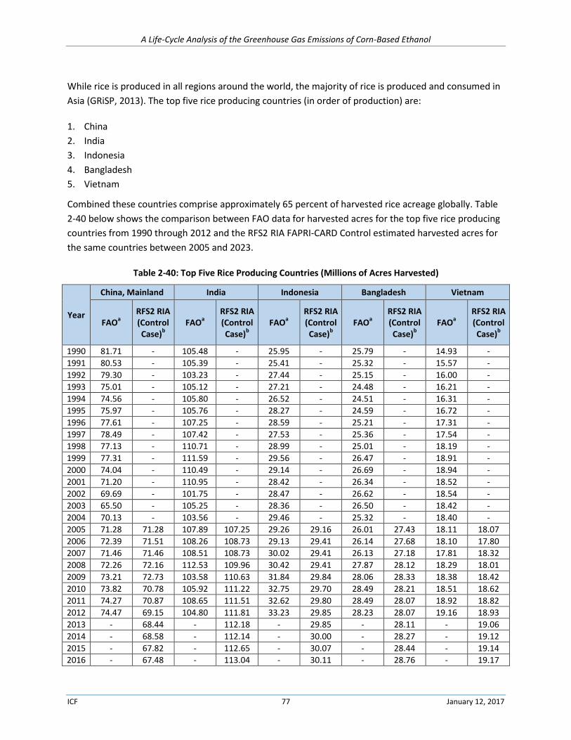
A Life-Cycle Analysis of the Greenhouse Gas Emissions of Corn-Based Ethanol
ICF 77 January 12, 2017
While rice is produced in all regions around the world, the majority of rice is produced and consumed in
Asia (GRiSP, 2013). The top five rice producing countries (in order of production) are:
1. China
2. India
3. Indonesia
4. Bangladesh
5. Vietnam
Combined these countries comprise approximately 65 percent of harvested rice acreage globally. Table
2-40 below shows the comparison between FAO data for harvested acres for the top five rice producing
countries from 1990 through 2012 and the RFS2 RIA FAPRI-CARD Control estimated harvested acres for
the same countries between 2005 and 2023.
Table 2-40: Top Five Rice Producing Countries (Millions of Acres Harvested)
Year
China, Mainland India Indonesia Bangladesh Vietnam
FAOa
RFS2 RIA (Control Case)
b
FAOa
RFS2 RIA (Control Case)
b
FAOa
RFS2 RIA (Control Case)
b
FAOa
RFS2 RIA (Control Case)
b
FAOa
RFS2 RIA (Control Case)
b
1990 81.71 - 105.48 - 25.95 - 25.79 - 14.93 -
1991 80.53 - 105.39 - 25.41 - 25.32 - 15.57 -
1992 79.30 - 103.23 - 27.44 - 25.15 - 16.00 -
1993 75.01 - 105.12 - 27.21 - 24.48 - 16.21 -
1994 74.56 - 105.80 - 26.52 - 24.51 - 16.31 -
1995 75.97 - 105.76 - 28.27 - 24.59 - 16.72 -
1996 77.61 - 107.25 - 28.59 - 25.21 - 17.31 -
1997 78.49 - 107.42 - 27.53 - 25.36 - 17.54 -
1998 77.13 - 110.71 - 28.99 - 25.01 - 18.19 -
1999 77.31 - 111.59 - 29.56 - 26.47 - 18.91 -
2000 74.04 - 110.49 - 29.14 - 26.69 - 18.94 -
2001 71.20 - 110.95 - 28.42 - 26.34 - 18.52 -
2002 69.69 - 101.75 - 28.47 - 26.62 - 18.54 -
2003 65.50 - 105.25 - 28.36 - 26.50 - 18.42 -
2004 70.13 - 103.56 - 29.46 - 25.32 - 18.40 -
2005 71.28 71.28 107.89 107.25 29.26 29.16 26.01 27.43 18.11 18.07
2006 72.39 71.51 108.26 108.73 29.13 29.41 26.14 27.68 18.10 17.80
2007 71.46 71.46 108.51 108.73 30.02 29.41 26.13 27.18 17.81 18.32
2008 72.26 72.16 112.53 109.96 30.42 29.41 27.87 28.12 18.29 18.01
2009 73.21 72.73 103.58 110.63 31.84 29.84 28.06 28.33 18.38 18.42
2010 73.82 70.78 105.92 111.22 32.75 29.70 28.49 28.21 18.51 18.62
2011 74.27 70.87 108.65 111.51 32.62 29.80 28.49 28.07 18.92 18.82
2012 74.47 69.15 104.80 111.81 33.23 29.85 28.23 28.07 19.16 18.93
2013 - 68.44 - 112.18 - 29.85 - 28.11 - 19.06
2014 - 68.58 - 112.14 - 30.00 - 28.27 - 19.12
2015 - 67.82 - 112.65 - 30.07 - 28.44 - 19.14
2016 - 67.48 - 113.04 - 30.11 - 28.76 - 19.17
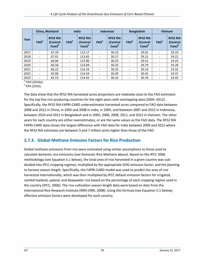
A Life-Cycle Analysis of the Greenhouse Gas Emissions of Corn-Based Ethanol
ICF 78 January 12, 2017
Year
China, Mainland India Indonesia Bangladesh Vietnam
FAOa
RFS2 RIA (Control Case)
b
FAOa
RFS2 RIA (Control Case)
b
FAOa
RFS2 RIA (Control Case)
b
FAOa
RFS2 RIA (Control Case)
b
FAOa
RFS2 RIA (Control Case)
b
2017 - 67.29 - 113.17 - 30.23 - 29.01 - 19.19
2018 - 67.01 - 113.65 - 30.17 - 29.22 - 19.22
2019 - 66.84 - 113.90 - 30.23 - 29.51 - 19.25
2020 - 66.56 - 114.09 - 30.25 - 29.79 - 19.28
2021 - 66.22 - 114.33 - 30.33 - 30.14 - 19.32
2022 - 65.80 - 114.59 - 30.30 - 30.42 - 19.37
2023 - 65.53 - 114.92 - 30.33 - 30.76 - 19.45 a FAO (2016a).
b EPA (2010).
The data show that the RFS2 RIA harvested acres projections are relatively close to the FAO estimates
for the top five rice producing countries for the eight years with overlapping data (2005–2012).
Specifically, the RFS2 RIA FAPRI-CARD underestimates harvested acres compared to FAO data between
2008 and 2012 in China, in 2005 and 2008 in India, in 2005, and between 2007 and 2012 in Indonesia,
between 2010 and 2012 in Bangladesh and in 2005, 2006, 2008, 2011, and 2012 in Vietnam. The other
years for each country are either overestimates, or are the same values as the FAO data. The RFS2 RIA
FAPRI-CARD data shows the largest difference with FAO data for India between 2009 and 2012 where
the RFS2 RIA estimates are between 3 and 7 million acres higher than those of the FAO.
2.7.3. Global Methane Emission Factors for Rice Production
Global methane emissions from rice were estimated using similar assumptions to those used to
calculate domestic rice emissions (see Domestic Rice Methane above). Based on the IPCC 2006
methodology (see Equation 5.1 below), the total area of rice harvested in a given country was sub-
divided into IPCC cropping regimes, multiplied by the appropriate GHG emission factor, and the planting
to harvest season length. Specifically, the FAPRI-CARD model was used to predict the area of rice
harvested internationally, which was then multiplied by IPCC default emission factors for irrigated,
rainfed lowland, upland, and deepwater rice based on the percentage of each cropping regime used in
the country (IPCC, 2006). The rice cultivation season length data were based on data from the
International Rice Research Institute (IRRI) (IRRI, 2008). Using this formula (see Equation 5.1 below),
effective emission factors were developed for each country.
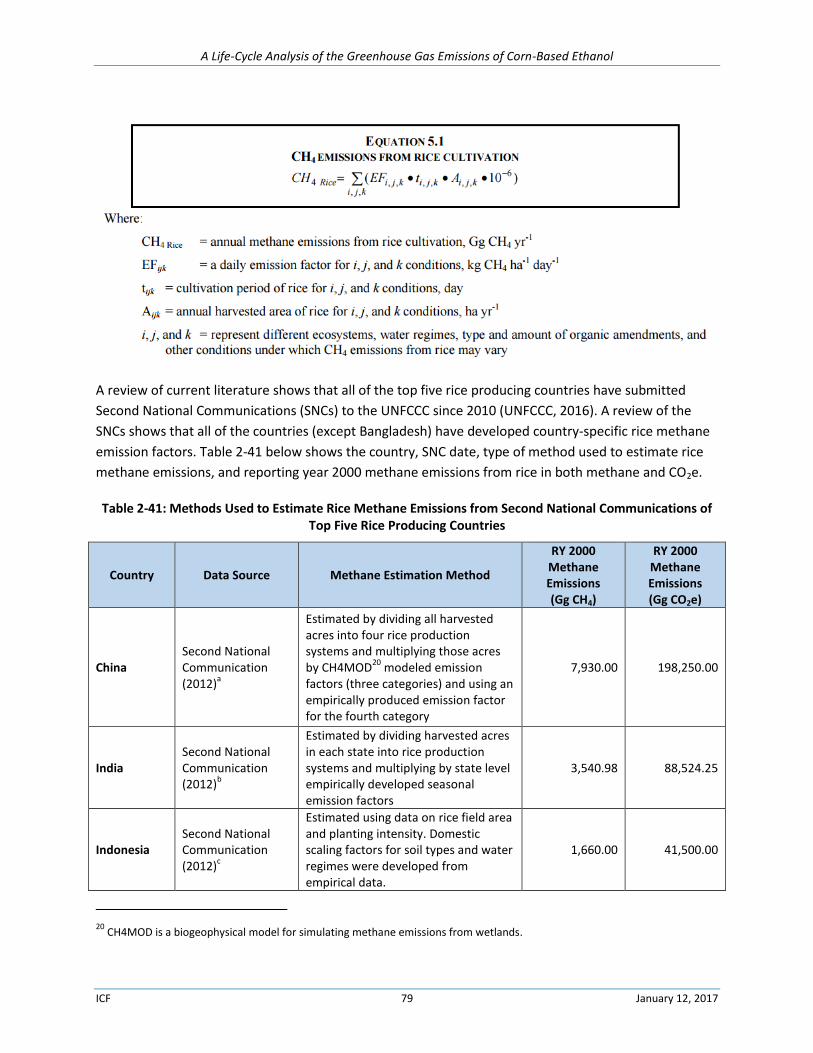
A Life-Cycle Analysis of the Greenhouse Gas Emissions of Corn-Based Ethanol
ICF 79 January 12, 2017
A review of current literature shows that all of the top five rice producing countries have submitted
Second National Communications (SNCs) to the UNFCCC since 2010 (UNFCCC, 2016). A review of the
SNCs shows that all of the countries (except Bangladesh) have developed country-specific rice methane
emission factors. Table 2-41 below shows the country, SNC date, type of method used to estimate rice
methane emissions, and reporting year 2000 methane emissions from rice in both methane and CO2e.
Table 2-41: Methods Used to Estimate Rice Methane Emissions from Second National Communications of Top Five Rice Producing Countries
Country Data Source Methane Estimation Method
RY 2000 Methane Emissions (Gg CH4)
RY 2000 Methane Emissions (Gg CO2e)
China Second National Communication (2012)
a
Estimated by dividing all harvested acres into four rice production systems and multiplying those acres by CH4MOD
20 modeled emission
factors (three categories) and using an empirically produced emission factor for the fourth category
7,930.00 198,250.00
India Second National Communication (2012)
b
Estimated by dividing harvested acres in each state into rice production systems and multiplying by state level empirically developed seasonal emission factors
3,540.98 88,524.25
Indonesia Second National Communication (2012)
c
Estimated using data on rice field area and planting intensity. Domestic scaling factors for soil types and water regimes were developed from empirical data.
1,660.00 41,500.00
20 CH4MOD is a biogeophysical model for simulating methane emissions from wetlands.
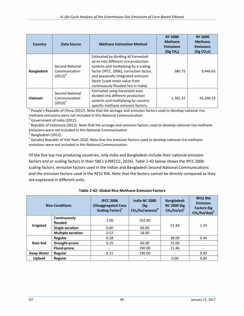
A Life-Cycle Analysis of the Greenhouse Gas Emissions of Corn-Based Ethanol
ICF 80 January 12, 2017
Country Data Source Methane Estimation Method
RY 2000 Methane Emissions (Gg CH4)
RY 2000 Methane Emissions (Gg CO2e)
Bangladesh Second National Communication (2012)
d
Estimated by dividing all harvested acres into different rice production systems and multiplying by a scaling factor (IPCC, 2006), correction factor, and seasonally integrated emission factor (used mean value from continuously flooded rice in India).
380.75 9,446.65
Vietnam Second National Communication (2010)
e
Estimated using harvested area divided into different production systems and multiplying by country-specific methane emission factors.
1,782.37 43,209.25
a People’s Republic of China (2012). Note that the acreage and emission factors used to develop national rice
methane emissions were not included in this National Communication. b Government of India (2012).
c Republic of Indonesia (2012). Note that the acreage and emission factors used to develop national rice methane
emissions were not included in this National Communication. d Bangladesh (2012).
e Socialist Republic of Viet Nam 2010. Note that the emission factors used to develop national rice methane
emissions were not included in this National Communication.
Of the five top rice producing countries, only India and Bangladesh include their national emission
factors and or scaling factors in their SNCs (UNFCCC, 2016). Table 2-42 below shows the IPCC 2006
scaling factors, emission factors used in the Indian and Bangladesh Second National Communications
and the emission factors used in the RFS2 RIA. Note that the factors cannot be directly compared as they
are expressed in different units.
Table 2-42: Global Rice Methane Emission Factors
Rice Conditions IPCC 2006
(Disaggregated Case Scaling Factor)
a
India NC 2000 (kg
CH4/ha/season)b
Bangladesh NC 2000 (kg CH4/ha/yr)
c
RFS2 RIA Emission
Factors (kg CH4/ha/day)
d
Irrigated
Continuously flooded
1.00 162.00
52.44 1.24 Single aeration 0.60 66.00
Multiple aeration 0.52 18.00
Rain-fed
Regular 0.28 - 28.00 0.44
Drought-prone 0.25 66.00 25.00 -
Flood-prone - 190.00 11.46 -
Deep Water Regular 0.31 190.00 - 0.49
Upland Regular - - 0.00 0.00
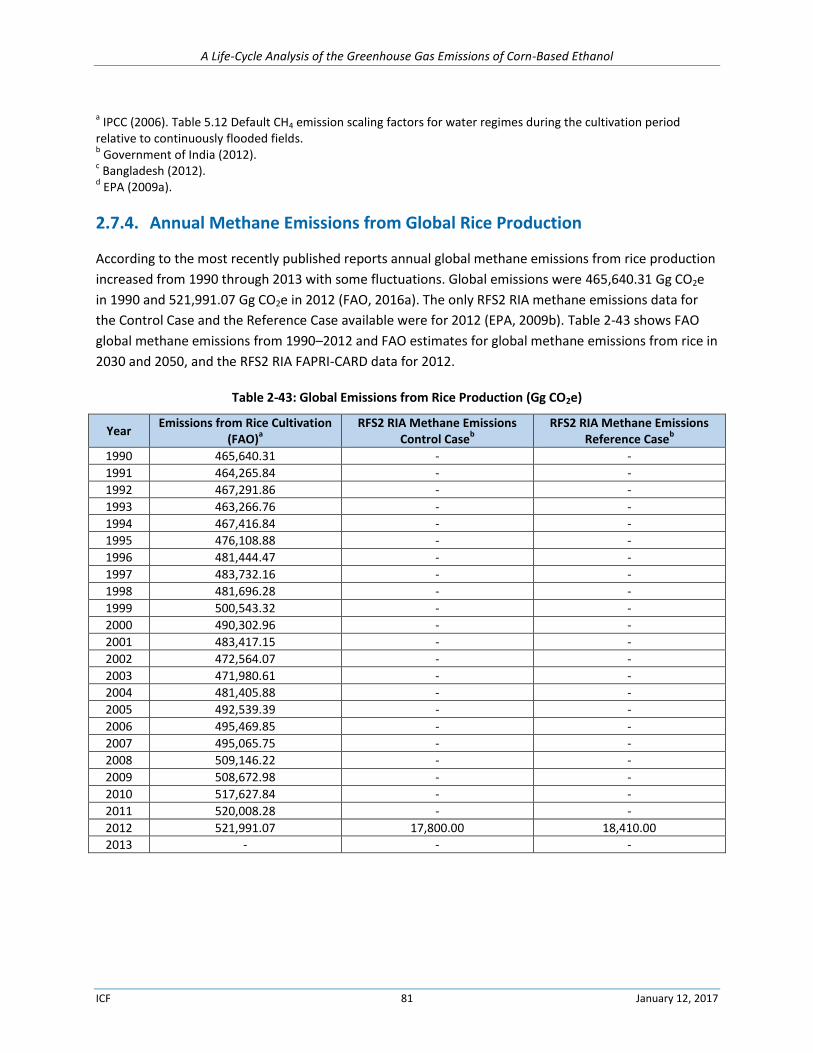
A Life-Cycle Analysis of the Greenhouse Gas Emissions of Corn-Based Ethanol
ICF 81 January 12, 2017
a IPCC (2006). Table 5.12 Default CH4 emission scaling factors for water regimes during the cultivation period
relative to continuously flooded fields. b Government of India (2012).
c Bangladesh (2012).
d EPA (2009a).
2.7.4. Annual Methane Emissions from Global Rice Production
According to the most recently published reports annual global methane emissions from rice production
increased from 1990 through 2013 with some fluctuations. Global emissions were 465,640.31 Gg CO2e
in 1990 and 521,991.07 Gg CO2e in 2012 (FAO, 2016a). The only RFS2 RIA methane emissions data for
the Control Case and the Reference Case available were for 2012 (EPA, 2009b). Table 2-43 shows FAO
global methane emissions from 1990–2012 and FAO estimates for global methane emissions from rice in
2030 and 2050, and the RFS2 RIA FAPRI-CARD data for 2012.
Table 2-43: Global Emissions from Rice Production (Gg CO2e)
Year Emissions from Rice Cultivation
(FAO)a
RFS2 RIA Methane Emissions Control Case
b RFS2 RIA Methane Emissions
Reference Caseb
1990 465,640.31 - -
1991 464,265.84 - -
1992 467,291.86 - -
1993 463,266.76 - -
1994 467,416.84 - -
1995 476,108.88 - -
1996 481,444.47 - -
1997 483,732.16 - -
1998 481,696.28 - -
1999 500,543.32 - -
2000 490,302.96 - -
2001 483,417.15 - -
2002 472,564.07 - -
2003 471,980.61 - -
2004 481,405.88 - -
2005 492,539.39 - -
2006 495,469.85 - -
2007 495,065.75 - -
2008 509,146.22 - -
2009 508,672.98 - -
2010 517,627.84 - -
2011 520,008.28 - -
2012 521,991.07 17,800.00 18,410.00
2013 - - -
A Life-Cycle Analysis of the Greenhouse Gas Emissions of Corn-Based Ethanol
ICF 82 January 12, 2017
a FAO (2016a).
b EPA (2009b).
The data show that similar to global harvested rice acreage, the FAO emissions21 increase from
465,640.31 Gg CO2e in 1990 to 521,991.07 Gg CO2e in 2012 (FAO, 2016a). The RFS2 RIA values for 2012
are approximately 3 percent of the FAO values.
2.7.5. Conclusions
A review of the current literature shows that global rice production and corresponding methane
emissions have increased between 1990 and 2012, with some fluctuation between years. The RFS2 RIA
FASOM data underestimates global harvested rice acreage. Emission factors used to develop the RFS2
RIA are based on Tier 1 IPCC 2006 guidelines. A review of the recent Second National Communications
(SNC) from the top 5 rice producing countries shows that most of the countries have now created their
own Tier 2 or Tier 3 country or region specific methane emission factors for rice. The RFS2 RIA emission
factors cannot be directly compared to the SNCs as they are expressed in different units. The total
projected 2012 global rice methane emissions from the RFS2 RIA are approximately three percent of
those from the FAO.
2.7.6. References: International Rice Methane
Government of the People’s Republic of Bangladesh, 2012. Second national communication of Bangladesh to the United Nations Framework Convention on Climate Change. http://unfccc.int/resource/docs/natc/bgdnc2.pdf
EPA, 2010c. FAPRI-CARD Results found in spreadsheet, “Memorandum to Docket. SUBJECT: Fapri-Card Lifecycle GHG (Greenhouse Gases) Analysis Results.xls” (Docket ID: EPA-HQ-OAR-2005-0161-3153). http://www.regulations.gov/#!documentDetail;D=EPA-HQ-OAR-2005-0161-3153
EPA, 2009a. Peer Review Report: International Agricultural Greenhouse Gas Emissions and Factors as provided to EPA to support its RFS2 rulemaking ID: EPA-HQ-OAR-2005-0161-1039 http://www.regulations.gov/#!documentDetail;D=EPA-HQ-OAR-2005-0
EPA, 2009b. GREET1.8c Results found in spreadsheet, “Renewable Fuel Lifecycle Greenhouse Gas Calculations (1).xls” (Docket ID: EPA-HQ-OAR-2005-0161-0950). http://www.regulations.gov/#!documentDetail;D=EPA-HQ-OAR-2005-0161-0950
FAO, 2016a. FAOSTAT: Emissions- Agriculture: Rice Cultivation. Food and Agriculture Organization of the United Nations. Accessed January 26, 2016. http://faostat3.fao.org/download/G1/GR/E
FAO, 2016b. Emissions- Agriculture: Rice cultivation. Food and Agriculture Organization of the United Nations. Accessed January 20, 2016. http://faostat3.fao.org/mes/methodology_list/E
21FAO state emissions are computed at Tier 1 following the Revised 1996 IPCC Guidelines for National GHG Inventories (IPCC,
1997) and the IPCC 2000 Good Practice Guidance and Uncertainty Management in National GHG Inventories (IPCC, 2000); available by country, with global coverage and relative to the period 1961-present, with annual updates, and projections for 2030 and 2050. (FAO, 2016b).
A Life-Cycle Analysis of the Greenhouse Gas Emissions of Corn-Based Ethanol
ICF 83 January 12, 2017
Gathorne-Hardy, A. (2013). Greenhouse gas emissions from rice (Vol. 3). RGTW Working Paper no. 3 http://www.southasia.ox.ac.uk/sites/sias/files/documents/GHG%20emissions%20from%20rice%20-%20%20working%20paper.pdf
Government of India, 2012. Second National Communication to the United Nations Framework Convention on Climate Change 2012. http://unfccc.int/resource/docs/natc/indnc2.pdf
GRiSP (Global Rice Science Partnership). 2013. Rice almanac, 4th edition. Los Baños, Philippines: International Rice Research Institute.
Hussain, S., Peng, S., Fahad, S., Khaliq, A., Huang, J., Cui, K., & Nie, L. (2015). Rice management interventions to mitigate greenhouse gas emissions: a review. Environmental Science and Pollution Research, 22(5), 3342-3360.
IPCC, 2006. Chapter 5: Cropland. In 2006 IPCC Guidelines for National Greenhouse Gas Inventories. Intergovernmental Panel on Climate Change. National Greenhouse Gas Inventories Programme, Kanagawa, Japan. http://www.ipcc-nggip.iges.or.jp/public/2006gl/
IRRI, 2008. International Rice Research Institute. www.irri.org
People’s Republic of China, 2012. Second National Communication on Climate Change of The People’s Republic of China 2012. http://unfccc.int/resource/docs/natc/chnnc2e.pdf
Republic of Indonesia, 2012. Indonesia Second National Communication under the United Nations Framework Convention on Climate Change (UNFCCC) 2012 http://unfccc.int/resource/docs/natc/indonc2.pdf
UNFCCC, 2016. Submitted National Communications from non-Annex I Parties. United Nationals Framework Convention on Climate Change. Accessed January 27, 2016. http://unfccc.int/national_reports/non-annex_i_natcom/submitted_natcom/items/653.php
USDA, ERS, 2015. Rice Yearbook 2015, Table 22: World rice supply and utilization. U.S. Department of Agriculture, Economic Research Service. http://www.ers.usda.gov/data-products/rice-yearbook-2015.aspx
Socialist Republic of Viet Nam, 2010. Viet Nam's second national communication to the United Nations Framework Convention on Climate Change. http://unfccc.int/resource/docs/natc/vnmnc02.pdf
2.8. Fuel and Feedstock Transport
EPA’s RFS2 RIA estimated that fuel and feedstock transportation accounted for less than 5 percent of
total life-cycle GHG emissions from corn ethanol (about 3.5 g CO2e/MJ). This estimation used GREET
emission factors for rail, barge and truck. In 2015, GREET researchers substantially expanded the
capabilities of the model’s truck transportation LCA. This expansion included five varieties of diesel and
gasoline freight vehicles. Beyond traditional fossil fuel vehicles, the update includes alternative fuel
vehicles for hybrid and hydraulic technologies: biodiesel, dimethyl ether, renewable diesel, compressed
natural gas, liquefied natural gas, liquefied petroleum gases, ethanol, and electricity (Cai et al., 2015).
Outside of GREET, researchers used economic input-output LCA (EIO-LCA) methodologies to determine
new life-cycle freight emission factors for rail, barge, truck, and air (Nealer et al., 2012). The
methodology determined these emission factors by analyzing industry inputs and outputs from over 400
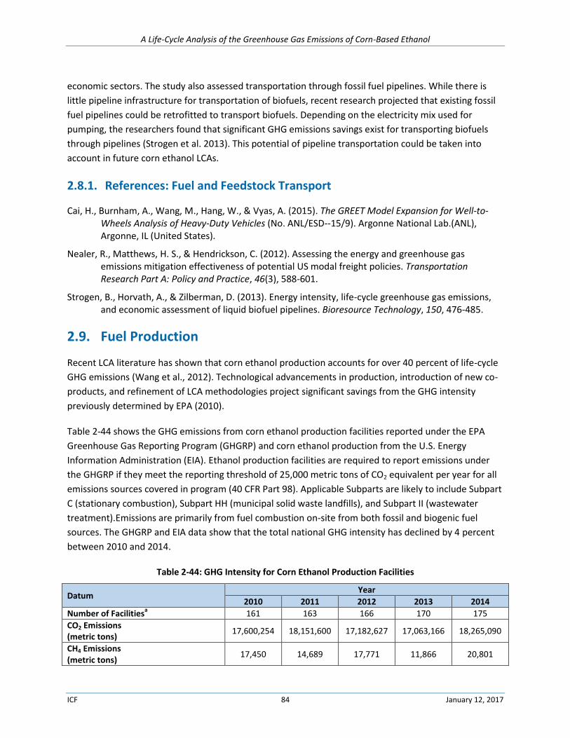
A Life-Cycle Analysis of the Greenhouse Gas Emissions of Corn-Based Ethanol
ICF 84 January 12, 2017
economic sectors. The study also assessed transportation through fossil fuel pipelines. While there is
little pipeline infrastructure for transportation of biofuels, recent research projected that existing fossil
fuel pipelines could be retrofitted to transport biofuels. Depending on the electricity mix used for
pumping, the researchers found that significant GHG emissions savings exist for transporting biofuels
through pipelines (Strogen et al. 2013). This potential of pipeline transportation could be taken into
account in future corn ethanol LCAs.
2.8.1. References: Fuel and Feedstock Transport
Cai, H., Burnham, A., Wang, M., Hang, W., & Vyas, A. (2015). The GREET Model Expansion for Well-to-Wheels Analysis of Heavy-Duty Vehicles (No. ANL/ESD--15/9). Argonne National Lab.(ANL), Argonne, IL (United States).
Nealer, R., Matthews, H. S., & Hendrickson, C. (2012). Assessing the energy and greenhouse gas emissions mitigation effectiveness of potential US modal freight policies. Transportation Research Part A: Policy and Practice, 46(3), 588-601.
Strogen, B., Horvath, A., & Zilberman, D. (2013). Energy intensity, life-cycle greenhouse gas emissions, and economic assessment of liquid biofuel pipelines. Bioresource Technology, 150, 476-485.
2.9. Fuel Production
Recent LCA literature has shown that corn ethanol production accounts for over 40 percent of life-cycle
GHG emissions (Wang et al., 2012). Technological advancements in production, introduction of new co-
products, and refinement of LCA methodologies project significant savings from the GHG intensity
previously determined by EPA (2010).
Table 2-44 shows the GHG emissions from corn ethanol production facilities reported under the EPA
Greenhouse Gas Reporting Program (GHGRP) and corn ethanol production from the U.S. Energy
Information Administration (EIA). Ethanol production facilities are required to report emissions under
the GHGRP if they meet the reporting threshold of 25,000 metric tons of CO2 equivalent per year for all
emissions sources covered in program (40 CFR Part 98). Applicable Subparts are likely to include Subpart
C (stationary combustion), Subpart HH (municipal solid waste landfills), and Subpart II (wastewater
treatment).Emissions are primarily from fuel combustion on-site from both fossil and biogenic fuel
sources. The GHGRP and EIA data show that the total national GHG intensity has declined by 4 percent
between 2010 and 2014.
Table 2-44: GHG Intensity for Corn Ethanol Production Facilities
Datum Year
2010 2011 2012 2013 2014
Number of Facilitiesa 161 163 166 170 175
CO2 Emissions (metric tons)
17,600,254 18,151,600 17,182,627 17,063,166 18,265,090
CH4 Emissions (metric tons)
17,450 14,689 17,771 11,866 20,801
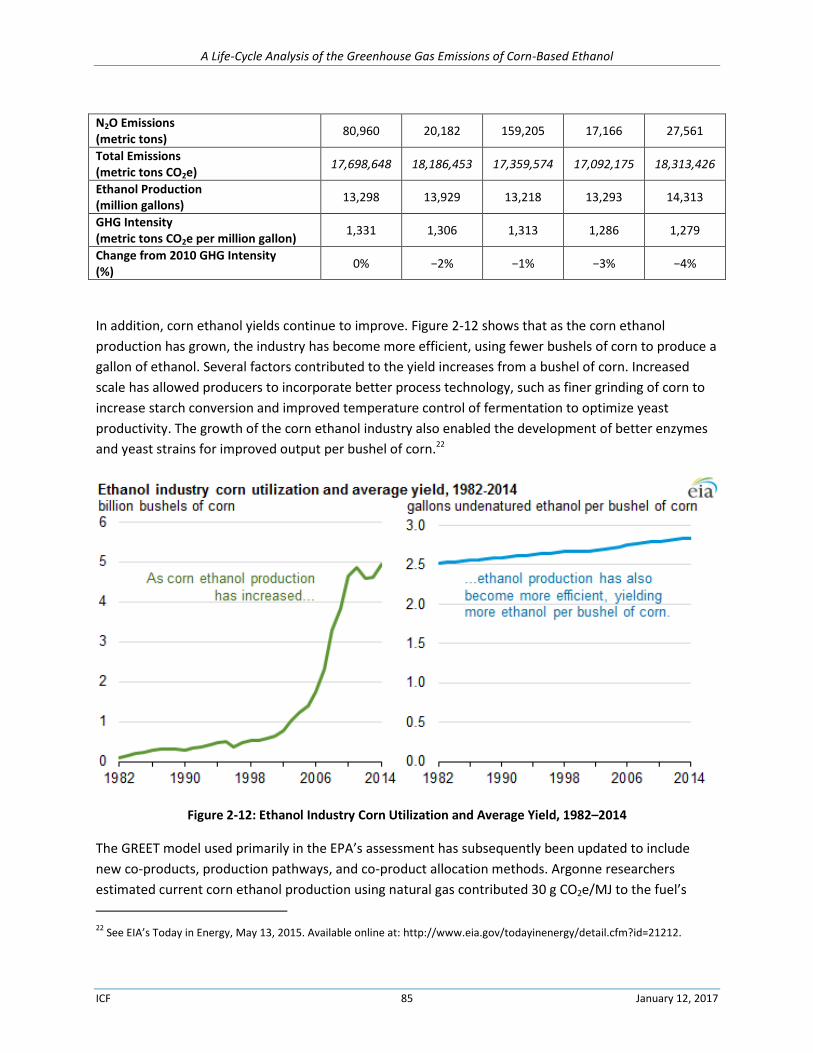
A Life-Cycle Analysis of the Greenhouse Gas Emissions of Corn-Based Ethanol
ICF 85 January 12, 2017
In addition, corn ethanol yields continue to improve. Figure 2-12 shows that as the corn ethanol
production has grown, the industry has become more efficient, using fewer bushels of corn to produce a
gallon of ethanol. Several factors contributed to the yield increases from a bushel of corn. Increased
scale has allowed producers to incorporate better process technology, such as finer grinding of corn to
increase starch conversion and improved temperature control of fermentation to optimize yeast
productivity. The growth of the corn ethanol industry also enabled the development of better enzymes
and yeast strains for improved output per bushel of corn.22
Figure 2-12: Ethanol Industry Corn Utilization and Average Yield, 1982–2014
The GREET model used primarily in the EPA’s assessment has subsequently been updated to include
new co-products, production pathways, and co-product allocation methods. Argonne researchers
estimated current corn ethanol production using natural gas contributed 30 g CO2e/MJ to the fuel’s
22 See EIA’s Today in Energy, May 13, 2015. Available online at: http://www.eia.gov/todayinenergy/detail.cfm?id=21212.
N2O Emissions (metric tons)
80,960 20,182 159,205 17,166 27,561
Total Emissions (metric tons CO2e)
17,698,648 18,186,453 17,359,574 17,092,175 18,313,426
Ethanol Production (million gallons)
13,298 13,929 13,218 13,293 14,313
GHG Intensity (metric tons CO2e per million gallon)
1,331 1,306 1,313 1,286 1,279
Change from 2010 GHG Intensity (%)
0% −2% −1% −3% −4%
A Life-Cycle Analysis of the Greenhouse Gas Emissions of Corn-Based Ethanol
ICF 86 January 12, 2017
well-to-wheels GHG intensity (Wang et al., 2012). This estimate is similar to the value projected for 2022
by the EPA (2010) report. The Argonne report acknowledged that major energy efficiency improvements
could be made to the system if corn and corn stover processes were combined, utilizing combined heat
and power (CHP) from the corn stover process.
The same research team produced a refined LCA of corn ethanol that detailed the benefits of dried
distillers grain (DGS) and corn oil recovery in ethanol production (Wang et al., 2015). The study applied
four different allocation techniques in determining the variations in effects of the co-products on the
final GHG intensity: marginal energy allocation, hybrid market-value allocation, process-level allocation,
and soy biodiesel displacement. This methodology estimated the life-cycle GHG intensity of corn ethanol
production to range between 15–20 g CO2e/MJ, a 33–50 percent reduction from the EPA report,
depending on the co-product handling method used. For the marginal and displacement methods,
ethanol production values are similar to Wang et al. 2012, but a DGS displacement credit reduces the
life-cycle emissions. The hybrid-market and process-level allocation methods do not use a displacement
credit, and allocate a share of the production burden to the DGS co-product based on the specific
method.
Boland and Unnasch (2014) projected significant reductions in life-cycle corn ethanol GHG intensity,
using the EPA (2010) report as a baseline. This study assessed a corn and corn stover ethanol production
pathway with 10 variations in fuel and co-products. The dry mill production variations using natural gas
ranged from 20–35 g CO2e/MJ. Substituting biomass in place of natural gas resulted in 10 g CO2e/MJ, a
67 percent reduction from the EPA report. The study projected these GHG intensities to decline by 8–20
percent from 2012–2022 due to efficiency improvements.
2.9.1. References: Fuel Production
Boland. S. and Unnasch. S. (2014) Carbon Intensity of Marginal Petroleum and Corn Ethanol Fuels. Life Cycle Associates Report LCA.6075.83.2014, Prepared for Renewable Fuels Association.
Wang, M., Han, J., Dunn, J. B., Cai, H., & Elgowainy, A. (2012). Well-to-wheels energy use and greenhouse gas emissions of ethanol from corn, sugarcane and cellulosic biomass for US use. Environmental Research Letters, 7(4), 045905.
Wang, Z., Dunn, J. B., Han, J., & Wang, M. Q. (2015). Influence of corn oil recovery on life-cycle greenhouse gas emissions of corn ethanol and corn oil biodiesel. Biotechnology for biofuels, 8(1), 1.
2.10. Tailpipe
About 19.64 pounds (8.91 kg) of carbon dioxide (CO2) are produced from burning a gallon of gasoline
that does not contain ethanol. Most of the retail gasoline now sold in the United States contains about
10 percent fuel ethanol (or E10) by volume. Burning a gallon of E10 produces about 17.68 pounds (8.02
kg) of CO2 that is emitted from the fossil fuel content. If the CO2 emissions from ethanol combustion are
A Life-Cycle Analysis of the Greenhouse Gas Emissions of Corn-Based Ethanol
ICF 87 January 12, 2017
considered, then about 18.95 pounds (8.60 kg) of CO2 are produced when a gallon of E10 is combusted.
About 12.73 pounds (5.77 kg) of CO2 are produced when a gallon of pure ethanol is combusted.23
The EPA (2010) report used the EPA’s motor vehicle emission simulator (MOVES) 2009 model to
estimate CH4 and N2O emissions from gasoline and diesel vehicles. The MOVES model derived emission
factors from federal GHG emission testing. The EPA has updated MOVES twice since the 2009 model in
2010 and 2014. The 2010 update included multiple improvements for gasoline and diesel GHG emission
rates for the following criteria (EPA, 2014):
Corporate Average Fuel Economy (CAFE) standards and projections for light duty vehicles from
2008–2016
Updated and projected energy usage rates for light and heavy-duty vehicles
Improved methane emission calculations based on total fuel hydrocarbons
The 2014 model further updated the gasoline/diesel emission factors to reflect changes in fuel economy
data. While these updates present opportunities for improvements in accuracy for future LCA models, it
should be noted that tailpipe emissions only represent about 1 percent of total life-cycle GHG emissions
from corn ethanol (EPA, 2010a).
2.10.1. References: Tailpipe
EPA, (2014). Greenhouse Gas and Energy Consumption Rates for On-road Vehicles: Updates for MOVES2014. http://www3.epa.gov/otaq/models/moves/documents/420r15003.pdf
23 See How much carbon dioxide is produced by burning gasoline and diesel fuel? Available online at: http://www.eia.gov/tools/faqs/faq.cfm?id=307&t=10.
A Life-Cycle Analysis of the Greenhouse Gas Emissions of Corn-Based Ethanol
ICF 88 January 12, 2017
3. Current GHG Emission Values for Each Emissions Source Category This chapter presents an assessment of the GHG footprint of corn-based ethanol today. For each
emission source category, we include a summary of the methods, data sources, and emissions
projection developed in the EPA RIA, describe the methods used here to quantify the contribution to
corn ethanol’s current GHG profile attributable to that category, and quantify that contribution.
The chapter is organized by emission category,specifically:
Domestic farm inputs and fertilizer N2O
Domestic land-use change
Domestic rice methane
Domestic livestock
International livestock
International land-use change
International farm inputs and fertilizer N2O
International rice methane
Fuel and feedstock transport
Fuel production
Tailpipe
Result of combining the current GHG emission category values
3.1. Domestic Farm Inputs and Fertilizer N2O
The domestic farm inputs evaluated in the EPA RIA include fertilizers, herbicides, pesticides, and on-site
fuel use. The fertilizers evaluated included nitrogen, phosphorous, potash, and lime. Representative
herbicides and pesticides were also included. On-site fuels included diesel, gasoline, natural gas, and
electricity. EPA also quantified N2O emissions due to application of synthetic fertilizers.
3.1.1. EPA RIA Methodology and Data Sources
The EPA RIA used the domestic agricultural inputs for fertilizer, pesticides, and energy use from the
Forestry and Agriculture Sector Optimization Model (FASOM) output (Adams et al., 2005). 24 The amount
of each input was determined based on the inputs required for the specified crops and the changes in
demand for those crops based on increased biofuel production. FASOM constructed crop budgets for 11
24 The Forestry and Agriculture Sector Optimization Model is a dynamic, partial equilibrium, sectoral model used to simulate potential future impacts of polices on land use, GHG fluxes, and commodity markets within the agricultural and forestry sectors. It has collaborators at Oregon State, Research Triangle Institute, Electric Power Research Institute, EPA, USDA, and USDA-Forest Service.
A Life-Cycle Analysis of the Greenhouse Gas Emissions of Corn-Based Ethanol
ICF 89 January 12, 2017
market regions, which varied by crop, management practice, and region. Within these crop budgets,
data on crop yield, fertilizer, pesticides, and fuels used were included. These budgets did not reflect
input or yield changes that may result in altered crop rotation patterns or the use of marginal land. The
energy use in FASOM represented the fuels used for grain drying. It was based on the assumptions that
17.5 gallons of propane and 9 kWh of electricity were required to remove 10 percentage points of
moisture from 100 bushels of grain. The total energy use per acre was determined by multiplying the
energy use per percentage point per yield unit for each crop that is dried (i.e., bushel of grain) by the
total number of percentage points to be removed and the yield per acre.
The emission factors used for the fertilizers and pesticides were from the Greenhouse Gas, Regulated
Emissions, and Energy use in Transportation (GREET) spreadsheet analysis tool developed by Argonne
National Laboratories. GREET version 1.8c was primarily used. The electricity emission factors represent
average U.S. grid electricity production and were also based on GREET (EPA, 2009).
The N2O emissions were based on different N-input sources including fertilizer application, nitrogen-
fixing crops such as soybeans, and crop residues. The N2O emissions from manure management systems
(and manure application) are addressed in the Domestic Livestock section. To model the domestic
impacts of N2O emissions from fertilizer application, Colorado State University’s CENTURY and DAYCENT
models were used. 25 The CENTURY and DAYCENT simulate plant-soil systems and simulates plant
production, soil carbon dynamics, soil nutrient dynamics and soil water and temperature. These
simulations account for all nitrogen inputs into the soil and provide regression equations with the
coefficients accounting for N2O estimates by region, crop type, irrigation status, and crop residue
treatment. The regression equations were then used to calculate the N2O emission per acre. FASOM was
used to evaluate the N2O emissions from crop residues and residue burning using IPCC guidelines and
assumed that 1 percent of nitrogen (N) residing in crop residues that remain on the field is emitted as
N2O emissions, following IPCC guidelines. These crop residues emissions estimates consider:
N content by crop based on yield,
Residue-to-crop ratio,
Percent dry matter,
Percentage of rice area burned in each state,
Burn and combustion efficiency, and
Percent of residue burned by crop.
25 Colorado State’s CENTURY and DAYCENT models are related models focused on nutrient cycling. The CENTURY model is a general model of plant-soil nutrient cycling which is being used to simulate carbon and nutrient dynamics for different types of ecosystems including grasslands, agricultural lands, forests, and savannas. The DAYCENT model simulates carbon and nitrogen fluxes through the ecosystem at daily time-step intervals.
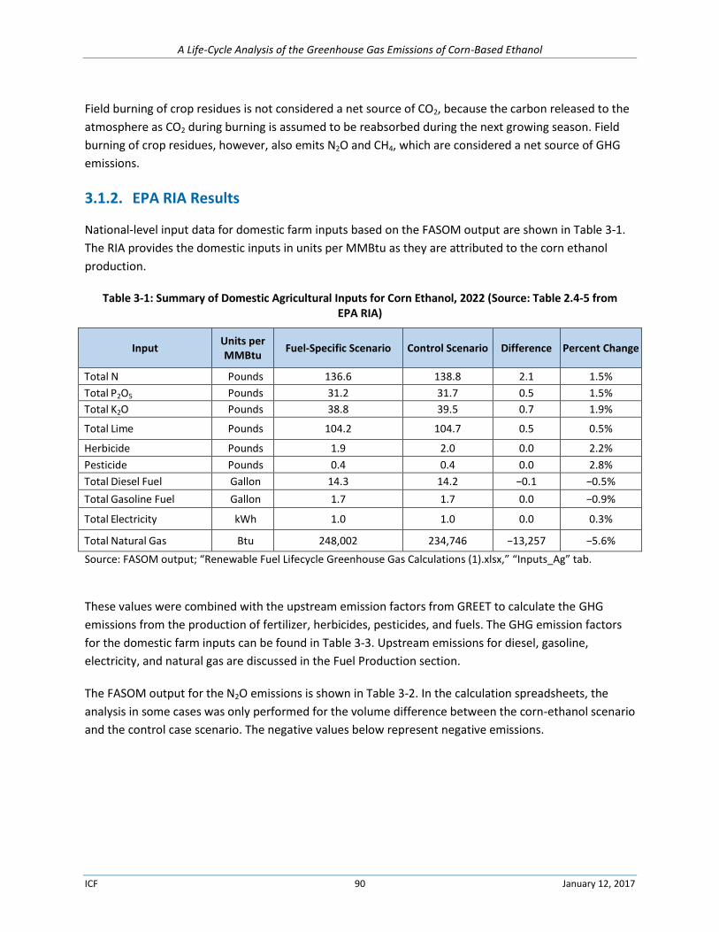
A Life-Cycle Analysis of the Greenhouse Gas Emissions of Corn-Based Ethanol
ICF 90 January 12, 2017
Field burning of crop residues is not considered a net source of CO2, because the carbon released to the
atmosphere as CO2 during burning is assumed to be reabsorbed during the next growing season. Field
burning of crop residues, however, also emits N2O and CH4, which are considered a net source of GHG
emissions.
3.1.2. EPA RIA Results
National-level input data for domestic farm inputs based on the FASOM output are shown in Table 3-1.
The RIA provides the domestic inputs in units per MMBtu as they are attributed to the corn ethanol
production.
Table 3-1: Summary of Domestic Agricultural Inputs for Corn Ethanol, 2022 (Source: Table 2.4-5 from EPA RIA)
Input Units per MMBtu
Fuel-Specific Scenario Control Scenario Difference Percent Change
Total N Pounds 136.6 138.8 2.1 1.5%
Total P2O5 Pounds 31.2 31.7 0.5 1.5%
Total K2O Pounds 38.8 39.5 0.7 1.9%
Total Lime Pounds 104.2 104.7 0.5 0.5%
Herbicide Pounds 1.9 2.0 0.0 2.2%
Pesticide Pounds 0.4 0.4 0.0 2.8%
Total Diesel Fuel Gallon 14.3 14.2 −0.1 −0.5%
Total Gasoline Fuel Gallon 1.7 1.7 0.0 −0.9%
Total Electricity kWh 1.0 1.0 0.0 0.3%
Total Natural Gas Btu 248,002 234,746 −13,257 −5.6%
Source: FASOM output; “Renewable Fuel Lifecycle Greenhouse Gas Calculations (1).xlsx,” “Inputs_Ag” tab.
These values were combined with the upstream emission factors from GREET to calculate the GHG
emissions from the production of fertilizer, herbicides, pesticides, and fuels. The GHG emission factors
for the domestic farm inputs can be found in Table 3-3. Upstream emissions for diesel, gasoline,
electricity, and natural gas are discussed in the Fuel Production section.
The FASOM output for the N2O emissions is shown in Table 3-2. In the calculation spreadsheets, the
analysis in some cases was only performed for the volume difference between the corn-ethanol scenario
and the control case scenario. The negative values below represent negative emissions.
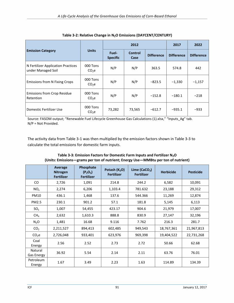
A Life-Cycle Analysis of the Greenhouse Gas Emissions of Corn-Based Ethanol
ICF 91 January 12, 2017
Table 3-2: Relative Change in N2O Emissions (DAYCENT/CENTURY)
Emission Category Units
2012 2017 2022
Fuel-Specific
Control Case
Difference Difference Difference
N Fertilizer Application Practices under Managed Soil
000 Tons CO2e
N/P N/P 363.5 574.8 442
Emissions from N Fixing Crops 000 Tons
CO2e N/P N/P −823.5 −1,330 −1,157
Emissions from Crop Residue Retention
000 Tons CO2e
N/P N/P −152.8 −180.1 −218
Domestic Fertilizer Use 000 Tons
CO2e 73,282 73,565 −612.7 −935.1 −933
Source: FASOM output; “Renewable Fuel Lifecycle Greenhouse Gas Calculations (1).xlsx,” “Inputs_Ag” tab. N/P = Not Provided.
The activity data from Table 3-1 was then multiplied by the emission factors shown in Table 3-3 to
calculate the total emissions for domestic farm inputs.
Table 3-3: Emission Factors for Domestic Farm Inputs and Fertilizer N2O (Units: Emissions—grams per ton of nutrient; Energy Use—MMBtu per ton of nutrient)
Average Nitrogen Fertilizer
Phosphate (P2O5)
Fertilizer
Potash (K2O) Fertilizer
Lime (CaCO3) Fertilizer
Herbicide Pesticide
CO 2,726 1,091 214.8 244.2 6,582 10,091
NOx 2,274 6,206 1,103.4 781.632 23,188 29,312
PM10 436.1 1,468 137.6 544.366 11,269 12,874
PM2.5 230.1 901.2 57.1 181.8 5,145 6,113
SOx 1,007 54,455 423.17 904.6 21,979 17,007
CH4 2,632 1,610.3 888.8 830.9 27,147 32,196
N2O 1,481 16.68 9.116 7.762 216.3 281.7
CO2 2,211,527 894,413 602,485 949,543 18,767,361 21,967,813
CO2e 2,726,048 933,401 623,976 969,398 19,404,522 22,731,268
Coal Energy
2.56 2.52 2.73 2.72 50.66 62.68
Natural Gas Energy
36.92 5.54 2.14 2.11 63.76 76.01
Petroleum Energy
1.67 3.49 2.23 1.63 114.89 134.39
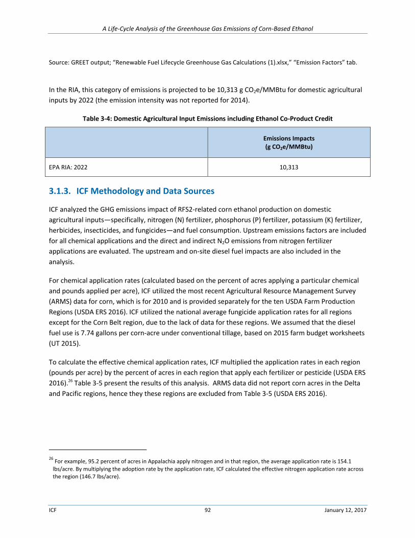
A Life-Cycle Analysis of the Greenhouse Gas Emissions of Corn-Based Ethanol
ICF 92 January 12, 2017
Source: GREET output; “Renewable Fuel Lifecycle Greenhouse Gas Calculations (1).xlsx,” “Emission Factors” tab.
In the RIA, this category of emissions is projected to be 10,313 g CO2e/MMBtu for domestic agricultural
inputs by 2022 (the emission intensity was not reported for 2014).
Table 3-4: Domestic Agricultural Input Emissions including Ethanol Co-Product Credit
Emissions Impacts (g CO2e/MMBtu)
EPA RIA: 2022 10,313
3.1.3. ICF Methodology and Data Sources
ICF analyzed the GHG emissions impact of RFS2-related corn ethanol production on domestic
agricultural inputs—specifically, nitrogen (N) fertilizer, phosphorus (P) fertilizer, potassium (K) fertilizer,
herbicides, insecticides, and fungicides—and fuel consumption. Upstream emissions factors are included
for all chemical applications and the direct and indirect N2O emissions from nitrogen fertilizer
applications are evaluated. The upstream and on-site diesel fuel impacts are also included in the
analysis.
For chemical application rates (calculated based on the percent of acres applying a particular chemical
and pounds applied per acre), ICF utilized the most recent Agricultural Resource Management Survey
(ARMS) data for corn, which is for 2010 and is provided separately for the ten USDA Farm Production
Regions (USDA ERS 2016). ICF utilized the national average fungicide application rates for all regions
except for the Corn Belt region, due to the lack of data for these regions. We assumed that the diesel
fuel use is 7.74 gallons per corn-acre under conventional tillage, based on 2015 farm budget worksheets
(UT 2015).
To calculate the effective chemical application rates, ICF multiplied the application rates in each region
(pounds per acre) by the percent of acres in each region that apply each fertilizer or pesticide (USDA ERS
2016).26 Table 3-5 present the results of this analysis. ARMS data did not report corn acres in the Delta
and Pacific regions, hence they these regions are excluded from Table 3-5 (USDA ERS 2016).
26 For example, 95.2 percent of acres in Appalachia apply nitrogen and in that region, the average application rate is 154.1
lbs/acre. By multiplying the adoption rate by the application rate, ICF calculated the effective nitrogen application rate across the region (146.7 lbs/acre).
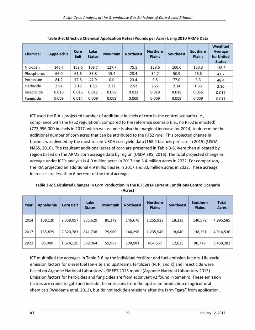
A Life-Cycle Analysis of the Greenhouse Gas Emissions of Corn-Based Ethanol
ICF 93 January 12, 2017
Table 3-5: Effective Chemical Application Rates (Pounds per Acre) Using 2010 ARMS Data
Chemical Appalachia Corn Belt
Lake States
Mountain Northeast Northern
Plains Southeast
Southern Plains
Weighted Average
for United States
Nitrogen 146.7 152.6 109.7 127.7 75.1 138.6 160.6 130.3 138.3
Phosphorus 66.0 61.6 35.8 15.4 23.4 34.7 50.9 26.8 47.7
Potassium 81.2 72.8 47.9 0.0 23.4 9.8 77.0 5.3 48.4
Herbicide 2.94 2.13 1.63 2.37 2.92 2.22 2.14 1.63 2.10
Insecticide 0.016 0.015 0.012 0.058 0.022 0.018 0.018 0.056 0.017
Fungicide 0.009 0.014 0.009 0.009 0.009 0.009 0.009 0.009 0.011
ICF used the RIA’s projected number of additional bushels of corn in the control scenario (i.e.,
compliance with the RFS2 regulation), compared to the reference scenario (i.e., no RFS2 is enacted)
(773,956,000 bushels in 2017, which we assume is also the marginal increase for 2014) to determine the
additional number of corn acres that can be attributed to the RFS2 rule. This projected change in
bushels was divided by the most recent USDA corn yield data (168.4 bushels per acre in 2015) (USDA
NASS, 2016). The resultant additional acres of corn are presented in Table 3-6, were then allocated by
region based on the ARMS corn acreage data by region (USDA ERS, 2016). The total projected change in
acreage under ICF’s analysis is 4.9 million acres in 2017 and 3.4 million acres in 2022. For comparison,
the RIA projected an additional 4.9 million acres in 2017 and 3.6 million acres in 2022. These acreage
increases are less than 6 percent of the total acreage.
Table 3-6: Calculated Changes in Corn Production in the ICF: 2014 Current Conditions Control Scenario (Acres)
Year Appalachia Corn Belt Lake
States Mountain Northeast
Northern Plains
Southeast Southern
Plains Total Acres
2014 138,120 2,359,057 855,620 81,279 146,676 1,255,923 18,338 140,572 4,995,585
2017 135,879 2,320,783 841,738 79,960 144,296 1,235,546 18,040 138,291 4,914,536
2022 95,090 1,624,126 589,064 55,957 100,981 864,657 12,625 96,778 3,439,282
ICF multiplied the acreages in Table 3-6 by the individual fertilizer and fuel emission factors. Life-cycle
emission factors for diesel fuel (on-site and upstream), fertilizers (N, P, and K) and insecticide were
based on Argonne National Laboratory’s GREET 2015 model (Argonne National Laboratory 2015).
Emission factors for herbicides and fungicides are from ecoinvent v2 found in SimaPro. These emission
factors are cradle to gate and include the emissions from the upstream production of agricultural
chemicals (Weidema et al. 2013), but do not include emissions after the farm “gate” from application.
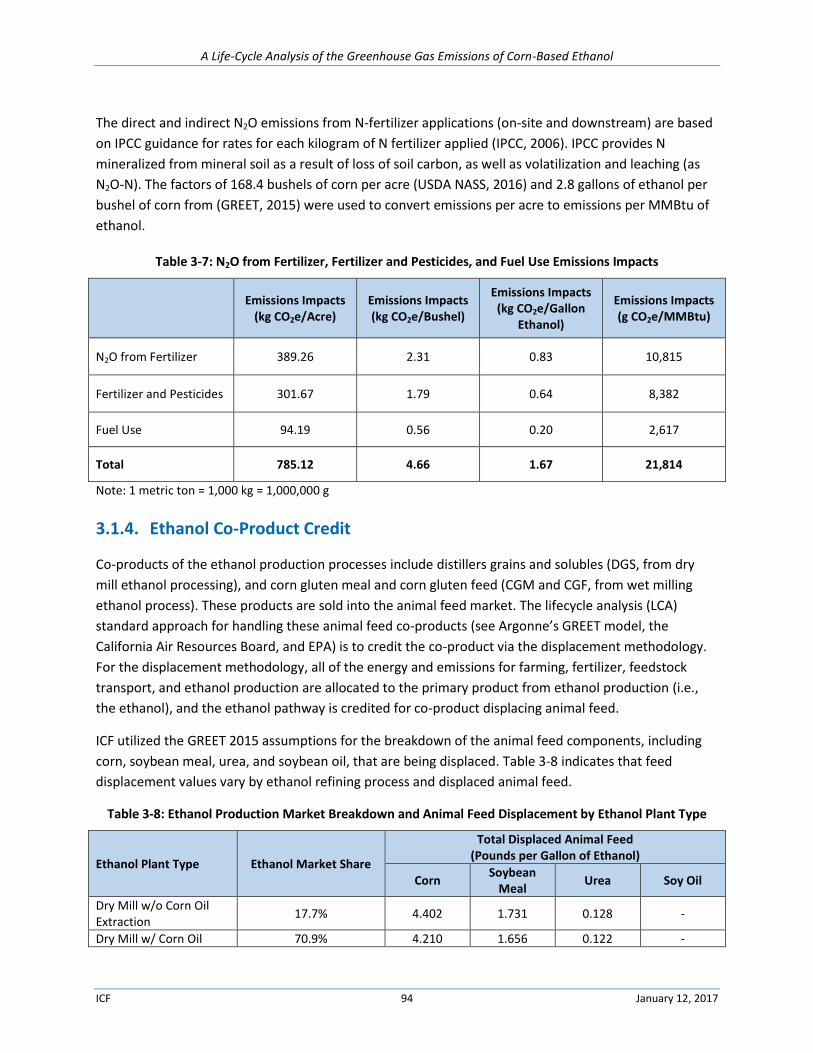
A Life-Cycle Analysis of the Greenhouse Gas Emissions of Corn-Based Ethanol
ICF 94 January 12, 2017
The direct and indirect N2O emissions from N-fertilizer applications (on-site and downstream) are based
on IPCC guidance for rates for each kilogram of N fertilizer applied (IPCC, 2006). IPCC provides N
mineralized from mineral soil as a result of loss of soil carbon, as well as volatilization and leaching (as
N2O-N). The factors of 168.4 bushels of corn per acre (USDA NASS, 2016) and 2.8 gallons of ethanol per
bushel of corn from (GREET, 2015) were used to convert emissions per acre to emissions per MMBtu of
ethanol.
Table 3-7: N2O from Fertilizer, Fertilizer and Pesticides, and Fuel Use Emissions Impacts
Emissions Impacts
(kg CO2e/Acre) Emissions Impacts (kg CO2e/Bushel)
Emissions Impacts (kg CO2e/Gallon
Ethanol)
Emissions Impacts (g CO2e/MMBtu)
N2O from Fertilizer 389.26 2.31 0.83 10,815
Fertilizer and Pesticides 301.67 1.79 0.64 8,382
Fuel Use 94.19 0.56 0.20 2,617
Total 785.12 4.66 1.67 21,814
Note: 1 metric ton = 1,000 kg = 1,000,000 g
3.1.4. Ethanol Co-Product Credit
Co-products of the ethanol production processes include distillers grains and solubles (DGS, from dry
mill ethanol processing), and corn gluten meal and corn gluten feed (CGM and CGF, from wet milling
ethanol process). These products are sold into the animal feed market. The lifecycle analysis (LCA)
standard approach for handling these animal feed co-products (see Argonne’s GREET model, the
California Air Resources Board, and EPA) is to credit the co-product via the displacement methodology.
For the displacement methodology, all of the energy and emissions for farming, fertilizer, feedstock
transport, and ethanol production are allocated to the primary product from ethanol production (i.e.,
the ethanol), and the ethanol pathway is credited for co-product displacing animal feed.
ICF utilized the GREET 2015 assumptions for the breakdown of the animal feed components, including
corn, soybean meal, urea, and soybean oil, that are being displaced. Table 3-8 indicates that feed
displacement values vary by ethanol refining process and displaced animal feed.
Table 3-8: Ethanol Production Market Breakdown and Animal Feed Displacement by Ethanol Plant Type
Ethanol Plant Type Ethanol Market Share
Total Displaced Animal Feed (Pounds per Gallon of Ethanol)
Corn Soybean
Meal Urea Soy Oil
Dry Mill w/o Corn Oil Extraction
17.7% 4.402 1.731 0.128 -
Dry Mill w/ Corn Oil 70.9% 4.210 1.656 0.122 -
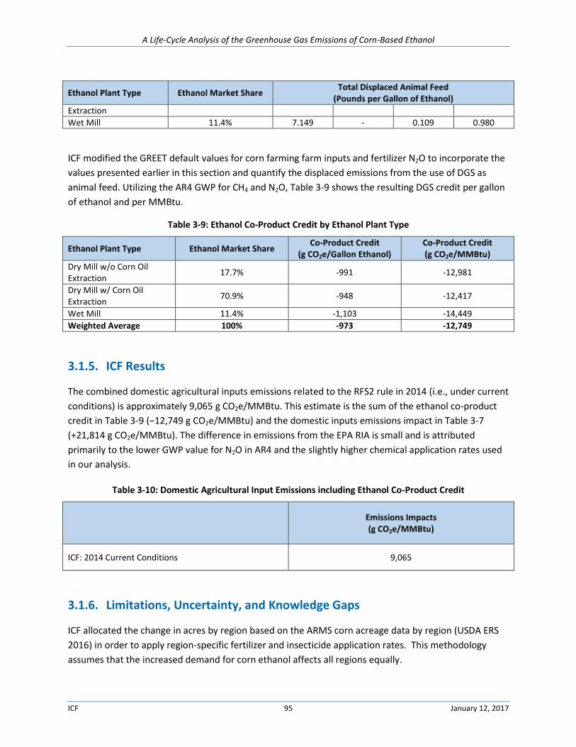
A Life-Cycle Analysis of the Greenhouse Gas Emissions of Corn-Based Ethanol
ICF 95 January 12, 2017
Ethanol Plant Type Ethanol Market Share Total Displaced Animal Feed
(Pounds per Gallon of Ethanol)
Extraction
Wet Mill 11.4% 7.149 - 0.109 0.980
ICF modified the GREET default values for corn farming farm inputs and fertilizer N2O to incorporate the
values presented earlier in this section and quantify the displaced emissions from the use of DGS as
animal feed. Utilizing the AR4 GWP for CH4 and N2O, Table 3-9 shows the resulting DGS credit per gallon
of ethanol and per MMBtu.
Table 3-9: Ethanol Co-Product Credit by Ethanol Plant Type
Ethanol Plant Type Ethanol Market Share Co-Product Credit
(g CO2e/Gallon Ethanol) Co-Product Credit (g CO2e/MMBtu)
Dry Mill w/o Corn Oil Extraction
17.7% -991 -12,981
Dry Mill w/ Corn Oil Extraction
70.9% -948 -12,417
Wet Mill 11.4% -1,103 -14,449
Weighted Average 100% -973 -12,749
3.1.5. ICF Results
The combined domestic agricultural inputs emissions related to the RFS2 rule in 2014 (i.e., under current
conditions) is approximately 9,065 g CO2e/MMBtu. This estimate is the sum of the ethanol co-product
credit in Table 3-9 (−12,749 g CO2e/MMBtu) and the domestic inputs emissions impact in Table 3-7
(+21,814 g CO2e/MMBtu). The difference in emissions from the EPA RIA is small and is attributed
primarily to the lower GWP value for N2O in AR4 and the slightly higher chemical application rates used
in our analysis.
Table 3-10: Domestic Agricultural Input Emissions including Ethanol Co-Product Credit
Emissions Impacts (g CO2e/MMBtu)
ICF: 2014 Current Conditions 9,065
3.1.6. Limitations, Uncertainty, and Knowledge Gaps
ICF allocated the change in acres by region based on the ARMS corn acreage data by region (USDA ERS
2016) in order to apply region-specific fertilizer and insecticide application rates. This methodology
assumes that the increased demand for corn ethanol affects all regions equally.
A Life-Cycle Analysis of the Greenhouse Gas Emissions of Corn-Based Ethanol
ICF 96 January 12, 2017
To model the energy associated with tillage and chemical application, ICF used a dataset that is specific
to Tennessee, however recognizes that other datasets, such as the ARMS data, could be used. The
University of Tennessee dataset provides the necessary granularity in energy used by activity. ICF
recognizes that crop budgets are based on recommendations.
Finally, this analysis did not include the emissions impacts from the current use of nitrogen inhibitors
and other advanced farming and agricultural practices. Potential emissions reductions from adoption of
these practices are considered in the projection scenarios developed in Chapter 4.
3.1.7. References: Domestic Farm Inputs and Fertilizer N2O
Adams, D., Alig, R., McCarl, B. A., & Murray, B. C. (2005). FASOMGHG Conceptual Structure and Specification: Documentation. Retrieved from http://agecon2.tamu.edu/people/faculty/mccarl-bruce/papers/1212FASOMGHG_doc.pdf
EPA. (2009, October 30). GREET. RFS2 FRM modified version of GREET1.8c Upstream Emissions Spreadsheet.
IPCC. (2006). 2006 IPCC Guidelines for National Greenhouse Gas Inventories, Prepared by the National Greenhouse Gas Inventories Programme, Eggleston H.S., Buendia L., Miwa K., Ngara T. and. Japan: IGES.
3.2. Domestic Land-Use Change
To model the land-use change within the United States, EPA used the FASOM model to project the land
conversions (Adams et al., 2005). In particular, EPA used the model to project land-use change from the
increase in corn ethanol production and the change in GHG emissions from the changes in land use.
3.2.1. EPA RIA Methodology and Data Sources
The FASOM model includes the land-use categories cropland, cropland pasture, forestland, forest
pasture, rangeland, developed land, and acres enrolled in the Conservation Reserve Program (CRP). The
model determines how much of each land-use category is actively used in production and how much is
idle during a specific time period.
Since the publication of the EPA RIA, FASOM has been updated to allow analysis across the forest and
agricultural sector combined as opposed to separate runs of the forest and agricultural sector
components. These model updates are not reflected in the RIA results. FASOM did not explicitly account
for the corn oil extracted from distillers grain. Since the RIA, the model has been modified to add this
pathway as part of the dry milling process. The original analysis is based on the assumption that by
2022, 70 percent of dry mill ethanol plants will withdraw corn oil via extraction, 20 percent will
withdraw corn oil via fractionation, and 10 percent will do neither (EPA, 2010a).
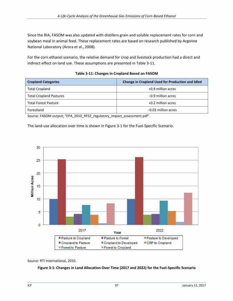
A Life-Cycle Analysis of the Greenhouse Gas Emissions of Corn-Based Ethanol
ICF 97 January 12, 2017
Since the RIA, FASOM was also updated with distillers grain and soluble replacement rates for corn and
soybean meal in animal feed. These replacement rates are based on research published by Argonne
National Laboratory (Arora et al., 2008).
For the corn ethanol scenario, the relative demand for crop and livestock production had a direct and
indirect effect on land use. These assumptions are presented in Table 3-11.
Table 3-11: Changes in Cropland Based on FASOM
Cropland Categories Change in Cropland Used for Production and Idled
Total Cropland +0.9 million acres
Total Cropland Pastures −0.9 million acres
Total Forest Pasture +0.2 million acres
Forestland −0.03 million acres
Source: FASOM output; “EPA_2010_RFS2_regulatory_impact_assessment.pdf”.
The land-use allocation over time is shown in Figure 3-1 for the Fuel-Specific Scenario.
Source: RTI International, 2010.
Figure 3-1: Changes in Land Allocation Over Time (2017 and 2022) for the Fuel-Specific Scenario
A Life-Cycle Analysis of the Greenhouse Gas Emissions of Corn-Based Ethanol
ICF 98 January 12, 2017
The land-use change is modelled across three phenomena:
1. Developed Land: FASOM assumed that developed land is of higher value than all other land
categories, the amount of developed land increased at a steady rate over time and the rate of
urbanization is assumed to be exogenous based on projections of population and income growth.
2. Carbon Sequestration: FASOM accounted for carbon storage in trees, understory, and litter within
both forests and plantations of woody biofuel feedstocks but excludes carbon stored in annually
cultivated crops. Changes in sequestration for land moved from the forestry and agricultural sectors
into developed land is tracked within FASOM.
3. Agricultural Land-Use Change GHG Emission Factors: FASOM agricultural land GHG emission factors
were updated with the DAYCENT/CENTURY model runs to reflect scientific updates at the time of
the model runs (RTI International, 2010).
To calculate the annualized timing of cumulative GHG emissions due to land-use change, all emissions
associated with agricultural land (CO2 and N2O from cropland, pastureland, and CRP land) and forestland
between 2000 and 2022 (CO2 from biomass, soil, and forest products) are summed as the emissions
from these categories accumulate over time. EPA’s RIA states, “The GHG emissions associated with
converting land into crop production would accumulate over time with the largest release occurring in
the first few years due to clearing with fire or biomass decay. After the land is converted, moderate
amounts of soil carbon would continue to be released for approximately 20 years. Furthermore, there
would be foregone sequestration associated with the fact that the forest would have continued to
sequester carbon had it not been cleared for approximately 80 years.”
3.2.2. EPA RIA Results
The aggregate GHG emissions from domestic land-use changes are a result of the difference in land-use
change and management practices in 2022 and dependent on changes in the land-use patterns that
occurred prior to 2022. FASOM generates GHG emissions estimates with land-use change for every five-
year period within the identified timeframe (Adams et al., 2005). Using these data, the EPA RIA
calculated the GHG emissions changes for corn ethanol and annualized the cumulative change (EPA,
2010a). The change in emissions is shown in Figure 3-2.
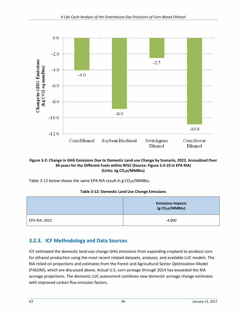
A Life-Cycle Analysis of the Greenhouse Gas Emissions of Corn-Based Ethanol
ICF 99 January 12, 2017
Figure 3-2: Change in GHG Emissions Due to Domestic Land-use Change by Scenario, 2022, Annualized Over 30 years for the Different Fuels within RFS2 (Source: Figure 2.4-19 in EPA RIA)
(Units: kg CO2e/MMBtu)
Table 3-12 below shows the same EPA RIA result in g CO2e/MMBtu.
Table 3-12: Domestic Land Use Change Emissions
Emissions Impacts (g CO2e/MMBtu)
EPA RIA: 2022 -4,000
3.2.3. ICF Methodology and Data Sources
ICF estimated the domestic land-use change GHG emissions from expanding cropland to produce corn
for ethanol production using the most recent related datasets, analyses, and available LUC models. The
RIA relied on projections and estimates from the Forest and Agricultural Sector Optimization Model
(FASOM), which are discussed above. Actual U.S. corn acreage through 2014 has exceeded the RIA
acreage projections. The domestic LUC assessment combines new domestic acreage change estimates
with improved carbon flux emission factors.
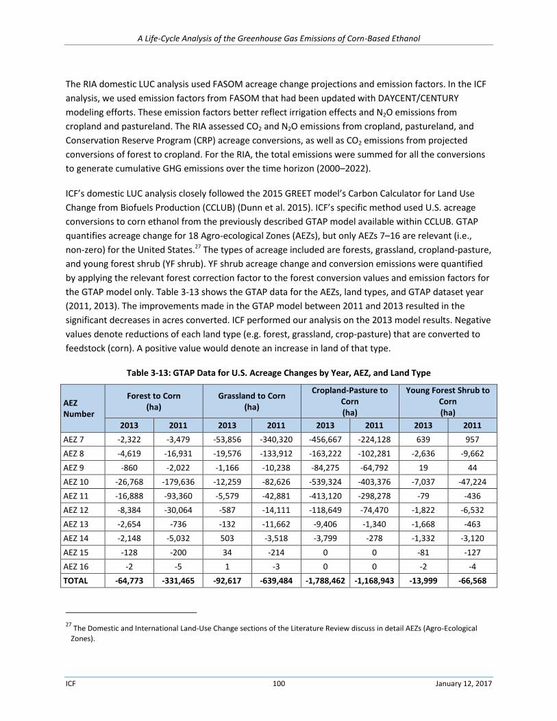
A Life-Cycle Analysis of the Greenhouse Gas Emissions of Corn-Based Ethanol
ICF 100 January 12, 2017
The RIA domestic LUC analysis used FASOM acreage change projections and emission factors. In the ICF
analysis, we used emission factors from FASOM that had been updated with DAYCENT/CENTURY
modeling efforts. These emission factors better reflect irrigation effects and N2O emissions from
cropland and pastureland. The RIA assessed CO2 and N2O emissions from cropland, pastureland, and
Conservation Reserve Program (CRP) acreage conversions, as well as CO2 emissions from projected
conversions of forest to cropland. For the RIA, the total emissions were summed for all the conversions
to generate cumulative GHG emissions over the time horizon (2000–2022).
ICF’s domestic LUC analysis closely followed the 2015 GREET model’s Carbon Calculator for Land Use
Change from Biofuels Production (CCLUB) (Dunn et al. 2015). ICF’s specific method used U.S. acreage
conversions to corn ethanol from the previously described GTAP model available within CCLUB. GTAP
quantifies acreage change for 18 Agro-ecological Zones (AEZs), but only AEZs 7–16 are relevant (i.e.,
non-zero) for the United States.27 The types of acreage included are forests, grassland, cropland-pasture,
and young forest shrub (YF shrub). YF shrub acreage change and conversion emissions were quantified
by applying the relevant forest correction factor to the forest conversion values and emission factors for
the GTAP model only. Table 3-13 shows the GTAP data for the AEZs, land types, and GTAP dataset year
(2011, 2013). The improvements made in the GTAP model between 2011 and 2013 resulted in the
significant decreases in acres converted. ICF performed our analysis on the 2013 model results. Negative
values denote reductions of each land type (e.g. forest, grassland, crop-pasture) that are converted to
feedstock (corn). A positive value would denote an increase in land of that type.
Table 3-13: GTAP Data for U.S. Acreage Changes by Year, AEZ, and Land Type
AEZ Number
Forest to Corn (ha)
Grassland to Corn (ha)
Cropland-Pasture to Corn (ha)
Young Forest Shrub to Corn (ha)
2013 2011 2013 2011 2013 2011 2013 2011
AEZ 7 -2,322 -3,479 -53,856 -340,320 -456,667 -224,128 639 957
AEZ 8 -4,619 -16,931 -19,576 -133,912 -163,222 -102,281 -2,636 -9,662
AEZ 9 -860 -2,022 -1,166 -10,238 -84,275 -64,792 19 44
AEZ 10 -26,768 -179,636 -12,259 -82,626 -539,324 -403,376 -7,037 -47,224
AEZ 11 -16,888 -93,360 -5,579 -42,881 -413,120 -298,278 -79 -436
AEZ 12 -8,384 -30,064 -587 -14,111 -118,649 -74,470 -1,822 -6,532
AEZ 13 -2,654 -736 -132 -11,662 -9,406 -1,340 -1,668 -463
AEZ 14 -2,148 -5,032 503 -3,518 -3,799 -278 -1,332 -3,120
AEZ 15 -128 -200 34 -214 0 0 -81 -127
AEZ 16 -2 -5 1 -3 0 0 -2 -4
TOTAL -64,773 -331,465 -92,617 -639,484 -1,788,462 -1,168,943 -13,999 -66,568
27 The Domestic and International Land-Use Change sections of the Literature Review discuss in detail AEZs (Agro-Ecological
Zones).
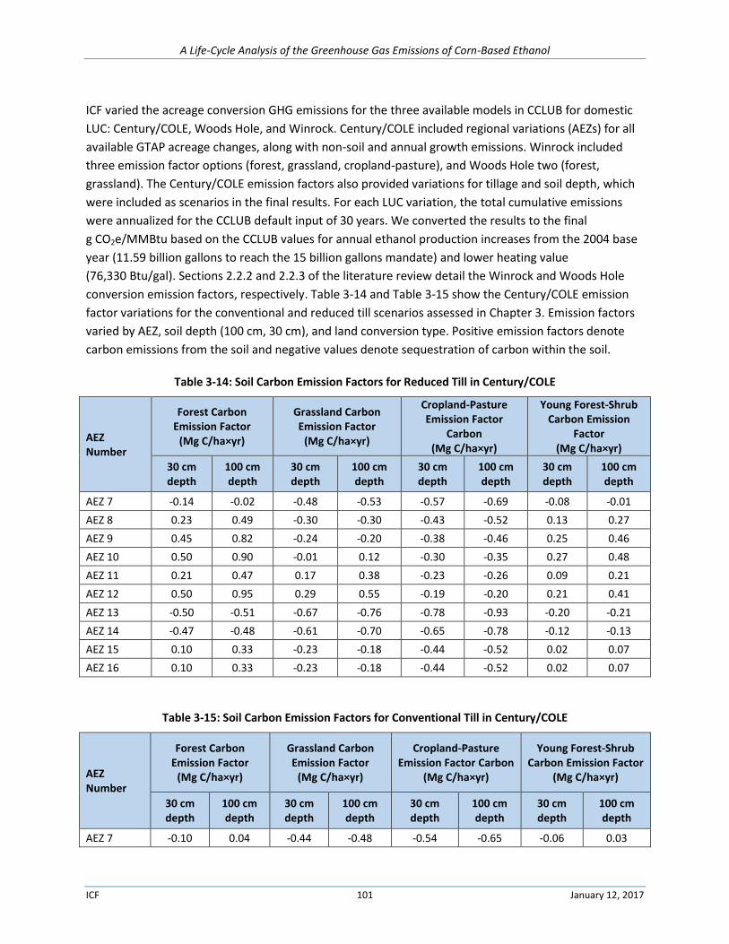
A Life-Cycle Analysis of the Greenhouse Gas Emissions of Corn-Based Ethanol
ICF 101 January 12, 2017
ICF varied the acreage conversion GHG emissions for the three available models in CCLUB for domestic
LUC: Century/COLE, Woods Hole, and Winrock. Century/COLE included regional variations (AEZs) for all
available GTAP acreage changes, along with non-soil and annual growth emissions. Winrock included
three emission factor options (forest, grassland, cropland-pasture), and Woods Hole two (forest,
grassland). The Century/COLE emission factors also provided variations for tillage and soil depth, which
were included as scenarios in the final results. For each LUC variation, the total cumulative emissions
were annualized for the CCLUB default input of 30 years. We converted the results to the final
g CO2e/MMBtu based on the CCLUB values for annual ethanol production increases from the 2004 base
year (11.59 billion gallons to reach the 15 billion gallons mandate) and lower heating value
(76,330 Btu/gal). Sections 2.2.2 and 2.2.3 of the literature review detail the Winrock and Woods Hole
conversion emission factors, respectively. Table 3-14 and Table 3-15 show the Century/COLE emission
factor variations for the conventional and reduced till scenarios assessed in Chapter 3. Emission factors
varied by AEZ, soil depth (100 cm, 30 cm), and land conversion type. Positive emission factors denote
carbon emissions from the soil and negative values denote sequestration of carbon within the soil.
Table 3-14: Soil Carbon Emission Factors for Reduced Till in Century/COLE
AEZ Number
Forest Carbon Emission Factor
(Mg C/ha×yr)
Grassland Carbon Emission Factor
(Mg C/ha×yr)
Cropland-Pasture Emission Factor
Carbon (Mg C/ha×yr)
Young Forest-Shrub Carbon Emission
Factor (Mg C/ha×yr)
30 cm depth
100 cm depth
30 cm depth
100 cm depth
30 cm depth
100 cm depth
30 cm depth
100 cm depth
AEZ 7 -0.14 -0.02 -0.48 -0.53 -0.57 -0.69 -0.08 -0.01
AEZ 8 0.23 0.49 -0.30 -0.30 -0.43 -0.52 0.13 0.27
AEZ 9 0.45 0.82 -0.24 -0.20 -0.38 -0.46 0.25 0.46
AEZ 10 0.50 0.90 -0.01 0.12 -0.30 -0.35 0.27 0.48
AEZ 11 0.21 0.47 0.17 0.38 -0.23 -0.26 0.09 0.21
AEZ 12 0.50 0.95 0.29 0.55 -0.19 -0.20 0.21 0.41
AEZ 13 -0.50 -0.51 -0.67 -0.76 -0.78 -0.93 -0.20 -0.21
AEZ 14 -0.47 -0.48 -0.61 -0.70 -0.65 -0.78 -0.12 -0.13
AEZ 15 0.10 0.33 -0.23 -0.18 -0.44 -0.52 0.02 0.07
AEZ 16 0.10 0.33 -0.23 -0.18 -0.44 -0.52 0.02 0.07
Table 3-15: Soil Carbon Emission Factors for Conventional Till in Century/COLE
AEZ Number
Forest Carbon Emission Factor
(Mg C/ha×yr)
Grassland Carbon Emission Factor
(Mg C/ha×yr)
Cropland-Pasture Emission Factor Carbon
(Mg C/ha×yr)
Young Forest-Shrub Carbon Emission Factor
(Mg C/ha×yr)
30 cm depth
100 cm depth
30 cm depth
100 cm depth
30 cm depth
100 cm depth
30 cm depth
100 cm depth
AEZ 7 -0.10 0.04 -0.44 -0.48 -0.54 -0.65 -0.06 0.03
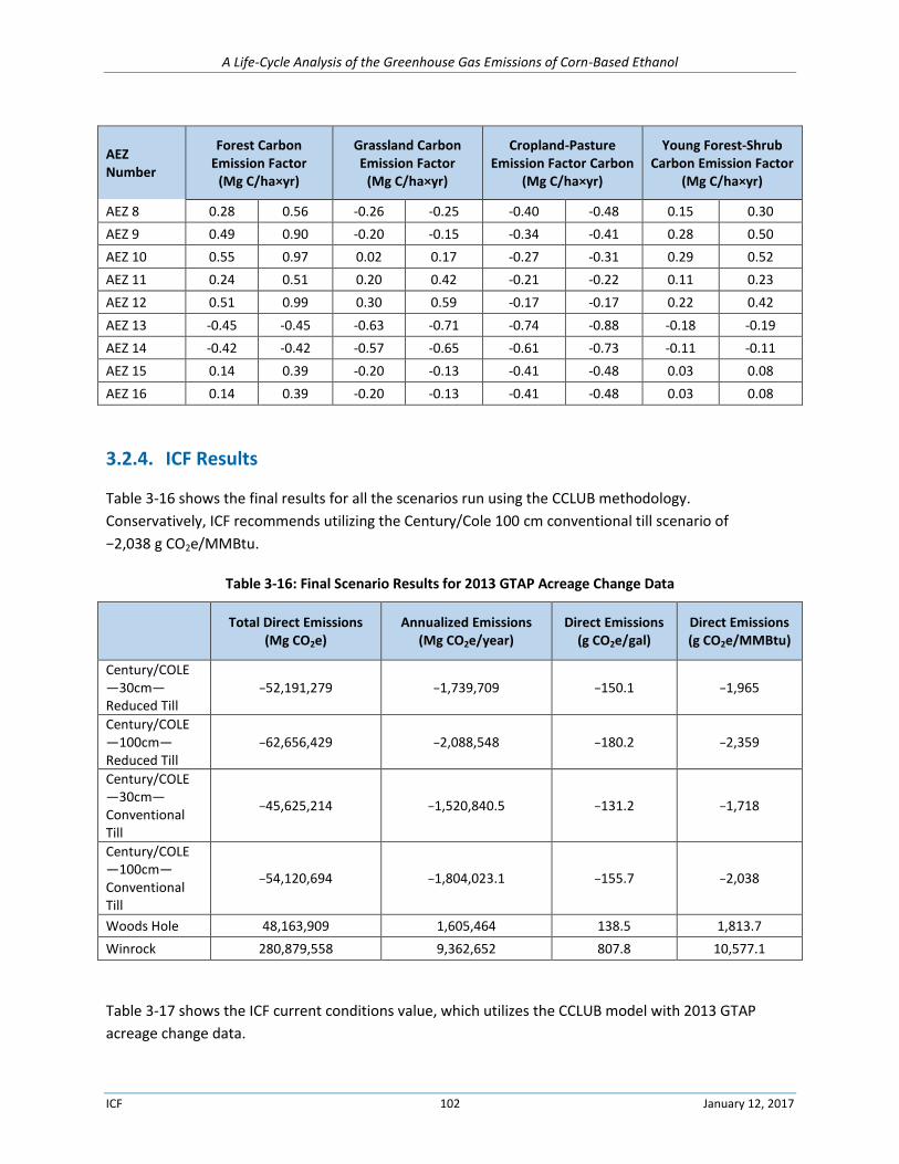
A Life-Cycle Analysis of the Greenhouse Gas Emissions of Corn-Based Ethanol
ICF 102 January 12, 2017
AEZ Number
Forest Carbon Emission Factor
(Mg C/ha×yr)
Grassland Carbon Emission Factor
(Mg C/ha×yr)
Cropland-Pasture Emission Factor Carbon
(Mg C/ha×yr)
Young Forest-Shrub Carbon Emission Factor
(Mg C/ha×yr)
AEZ 8 0.28 0.56 -0.26 -0.25 -0.40 -0.48 0.15 0.30
AEZ 9 0.49 0.90 -0.20 -0.15 -0.34 -0.41 0.28 0.50
AEZ 10 0.55 0.97 0.02 0.17 -0.27 -0.31 0.29 0.52
AEZ 11 0.24 0.51 0.20 0.42 -0.21 -0.22 0.11 0.23
AEZ 12 0.51 0.99 0.30 0.59 -0.17 -0.17 0.22 0.42
AEZ 13 -0.45 -0.45 -0.63 -0.71 -0.74 -0.88 -0.18 -0.19
AEZ 14 -0.42 -0.42 -0.57 -0.65 -0.61 -0.73 -0.11 -0.11
AEZ 15 0.14 0.39 -0.20 -0.13 -0.41 -0.48 0.03 0.08
AEZ 16 0.14 0.39 -0.20 -0.13 -0.41 -0.48 0.03 0.08
3.2.4. ICF Results
Table 3-16 shows the final results for all the scenarios run using the CCLUB methodology.
Conservatively, ICF recommends utilizing the Century/Cole 100 cm conventional till scenario of
−2,038 g CO2e/MMBtu.
Table 3-16: Final Scenario Results for 2013 GTAP Acreage Change Data
Total Direct Emissions
(Mg CO2e) Annualized Emissions
(Mg CO2e/year) Direct Emissions
(g CO2e/gal) Direct Emissions (g CO2e/MMBtu)
Century/COLE—30cm—Reduced Till
−52,191,279 −1,739,709 −150.1 −1,965
Century/COLE—100cm—Reduced Till
−62,656,429 −2,088,548 −180.2 −2,359
Century/COLE—30cm—Conventional Till
−45,625,214 −1,520,840.5 −131.2 −1,718
Century/COLE—100cm—Conventional Till
−54,120,694 −1,804,023.1 −155.7 −2,038
Woods Hole 48,163,909 1,605,464 138.5 1,813.7
Winrock 280,879,558 9,362,652 807.8 10,577.1
Table 3-17 shows the ICF current conditions value, which utilizes the CCLUB model with 2013 GTAP
acreage change data.
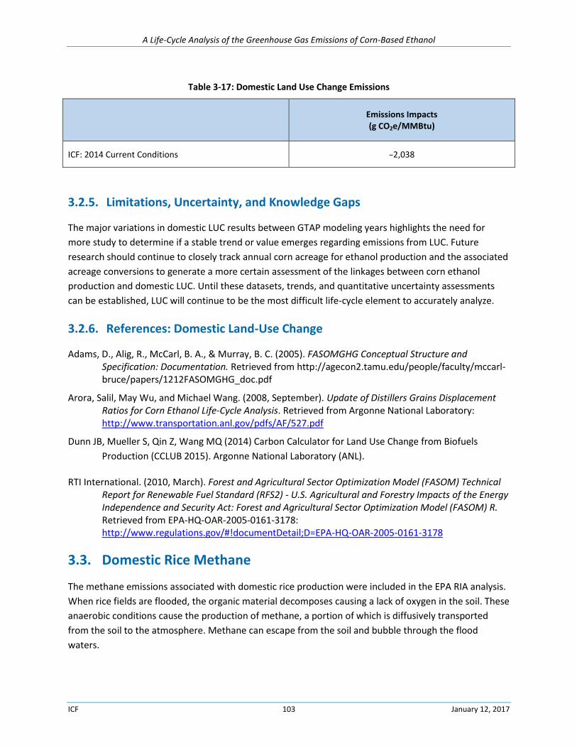
A Life-Cycle Analysis of the Greenhouse Gas Emissions of Corn-Based Ethanol
ICF 103 January 12, 2017
Table 3-17: Domestic Land Use Change Emissions
Emissions Impacts (g CO2e/MMBtu)
ICF: 2014 Current Conditions −2,038
3.2.5. Limitations, Uncertainty, and Knowledge Gaps
The major variations in domestic LUC results between GTAP modeling years highlights the need for
more study to determine if a stable trend or value emerges regarding emissions from LUC. Future
research should continue to closely track annual corn acreage for ethanol production and the associated
acreage conversions to generate a more certain assessment of the linkages between corn ethanol
production and domestic LUC. Until these datasets, trends, and quantitative uncertainty assessments
can be established, LUC will continue to be the most difficult life-cycle element to accurately analyze.
3.2.6. References: Domestic Land-Use Change
Adams, D., Alig, R., McCarl, B. A., & Murray, B. C. (2005). FASOMGHG Conceptual Structure and Specification: Documentation. Retrieved from http://agecon2.tamu.edu/people/faculty/mccarl-bruce/papers/1212FASOMGHG_doc.pdf
Arora, Salil, May Wu, and Michael Wang. (2008, September). Update of Distillers Grains Displacement Ratios for Corn Ethanol Life-Cycle Analysis. Retrieved from Argonne National Laboratory: http://www.transportation.anl.gov/pdfs/AF/527.pdf
Dunn JB, Mueller S, Qin Z, Wang MQ (2014) Carbon Calculator for Land Use Change from Biofuels
Production (CCLUB 2015). Argonne National Laboratory (ANL).
RTI International. (2010, March). Forest and Agricultural Sector Optimization Model (FASOM) Technical Report for Renewable Fuel Standard (RFS2) - U.S. Agricultural and Forestry Impacts of the Energy Independence and Security Act: Forest and Agricultural Sector Optimization Model (FASOM) R. Retrieved from EPA-HQ-OAR-2005-0161-3178: http://www.regulations.gov/#!documentDetail;D=EPA-HQ-OAR-2005-0161-3178
3.3. Domestic Rice Methane
The methane emissions associated with domestic rice production were included in the EPA RIA analysis.
When rice fields are flooded, the organic material decomposes causing a lack of oxygen in the soil. These
anaerobic conditions cause the production of methane, a portion of which is diffusively transported
from the soil to the atmosphere. Methane can escape from the soil and bubble through the flood
waters.
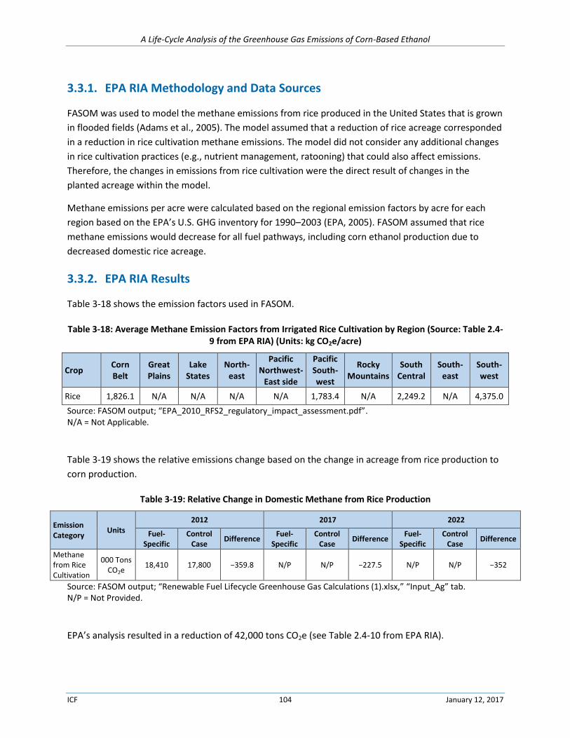
A Life-Cycle Analysis of the Greenhouse Gas Emissions of Corn-Based Ethanol
ICF 104 January 12, 2017
3.3.1. EPA RIA Methodology and Data Sources
FASOM was used to model the methane emissions from rice produced in the United States that is grown
in flooded fields (Adams et al., 2005). The model assumed that a reduction of rice acreage corresponded
in a reduction in rice cultivation methane emissions. The model did not consider any additional changes
in rice cultivation practices (e.g., nutrient management, ratooning) that could also affect emissions.
Therefore, the changes in emissions from rice cultivation were the direct result of changes in the
planted acreage within the model.
Methane emissions per acre were calculated based on the regional emission factors by acre for each
region based on the EPA’s U.S. GHG inventory for 1990–2003 (EPA, 2005). FASOM assumed that rice
methane emissions would decrease for all fuel pathways, including corn ethanol production due to
decreased domestic rice acreage.
3.3.2. EPA RIA Results
Table 3-18 shows the emission factors used in FASOM.
Table 3-18: Average Methane Emission Factors from Irrigated Rice Cultivation by Region (Source: Table 2.4-9 from EPA RIA) (Units: kg CO2e/acre)
Crop Corn Belt
Great Plains
Lake States
North-east
Pacific Northwest-
East side
Pacific South-west
Rocky Mountains
South Central
South-east
South-west
Rice 1,826.1 N/A N/A N/A N/A 1,783.4 N/A 2,249.2 N/A 4,375.0
Source: FASOM output; “EPA_2010_RFS2_regulatory_impact_assessment.pdf”. N/A = Not Applicable.
Table 3-19 shows the relative emissions change based on the change in acreage from rice production to
corn production.
Table 3-19: Relative Change in Domestic Methane from Rice Production
Emission Category
Units 2012 2017 2022
Fuel-Specific
Control Case
Difference Fuel-
Specific Control
Case Difference
Fuel-Specific
Control Case
Difference
Methane from Rice Cultivation
000 Tons CO2e
18,410 17,800 −359.8 N/P N/P −227.5 N/P N/P −352
Source: FASOM output; “Renewable Fuel Lifecycle Greenhouse Gas Calculations (1).xlsx,” “Input_Ag” tab. N/P = Not Provided.
EPA’s analysis resulted in a reduction of 42,000 tons CO2e (see Table 2.4-10 from EPA RIA).
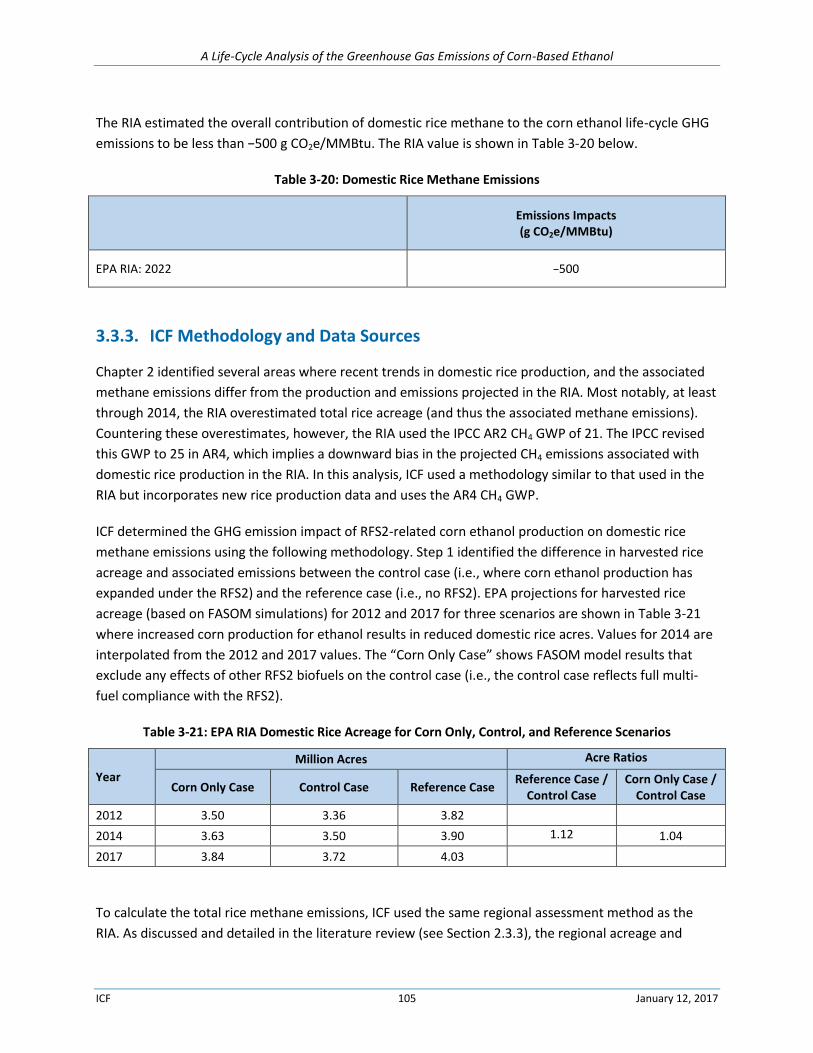
A Life-Cycle Analysis of the Greenhouse Gas Emissions of Corn-Based Ethanol
ICF 105 January 12, 2017
The RIA estimated the overall contribution of domestic rice methane to the corn ethanol life-cycle GHG
emissions to be less than −500 g CO2e/MMBtu. The RIA value is shown in Table 3-20 below.
Table 3-20: Domestic Rice Methane Emissions
Emissions Impacts (g CO2e/MMBtu)
EPA RIA: 2022 −500
3.3.3. ICF Methodology and Data Sources
Chapter 2 identified several areas where recent trends in domestic rice production, and the associated
methane emissions differ from the production and emissions projected in the RIA. Most notably, at least
through 2014, the RIA overestimated total rice acreage (and thus the associated methane emissions).
Countering these overestimates, however, the RIA used the IPCC AR2 CH4 GWP of 21. The IPCC revised
this GWP to 25 in AR4, which implies a downward bias in the projected CH4 emissions associated with
domestic rice production in the RIA. In this analysis, ICF used a methodology similar to that used in the
RIA but incorporates new rice production data and uses the AR4 CH4 GWP.
ICF determined the GHG emission impact of RFS2-related corn ethanol production on domestic rice
methane emissions using the following methodology. Step 1 identified the difference in harvested rice
acreage and associated emissions between the control case (i.e., where corn ethanol production has
expanded under the RFS2) and the reference case (i.e., no RFS2). EPA projections for harvested rice
acreage (based on FASOM simulations) for 2012 and 2017 for three scenarios are shown in Table 3-21
where increased corn production for ethanol results in reduced domestic rice acres. Values for 2014 are
interpolated from the 2012 and 2017 values. The “Corn Only Case” shows FASOM model results that
exclude any effects of other RFS2 biofuels on the control case (i.e., the control case reflects full multi-
fuel compliance with the RFS2).
Table 3-21: EPA RIA Domestic Rice Acreage for Corn Only, Control, and Reference Scenarios
Year
Million Acres Acre Ratios
Corn Only Case Control Case Reference Case Reference Case /
Control Case Corn Only Case /
Control Case
2012 3.50 3.36 3.82
2014 3.63 3.50 3.90 1.12 1.04
2017 3.84 3.72 4.03
To calculate the total rice methane emissions, ICF used the same regional assessment method as the
RIA. As discussed and detailed in the literature review (see Section 2.3.3), the regional acreage and
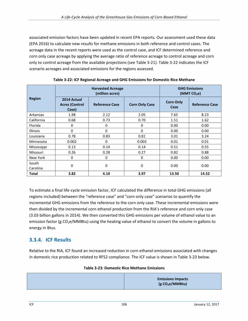
A Life-Cycle Analysis of the Greenhouse Gas Emissions of Corn-Based Ethanol
ICF 106 January 12, 2017
associated emission factors have been updated in recent EPA reports. Our assessment used these data
(EPA 2016) to calculate new results for methane emissions in both reference and control cases. The
acreage data in the recent reports were used as the control case, and ICF determined reference and
corn only case acreage by applying the average ratio of reference acreage to control acreage and corn
only to control acreage from the available projections (see Table 3-21). Table 3-22 indicates the ICF
scenario acreages and associated emissions for the regions assessed.
Table 3-22: ICF Regional Acreage and GHG Emissions for Domestic Rice Methane
Region
Harvested Acreage (million acres)
GHG Emissions (MMT CO2e)
2014 Actual Acres (Control
Case) Reference Case Corn Only Case
Corn Only Case
Reference Case
Arkansas 1.98 2.12 2.05 7.65 8.23
California 0.68 0.73 0.70 1.51 1.62
Florida 0 0 0 0.00 0.00
Illinois 0 0 0 0.00 0.00
Louisiana 0.78 0.83 0.81 3.01 3.24
Minnesota 0.002 0 0.003 0.01 0.01
Mississippi 0.13 0.14 0.14 0.51 0.55
Missouri 0.26 0.28 0.27 0.82 0.88
New York 0 0 0 0.00 0.00
South Carolina
0 0 0 0.00 0.00
Total 3.82 4.10 3.97 13.50 14.52
To estimate a final life-cycle emission factor, ICF calculated the difference in total GHG emissions (all
regions included) between the “reference case” and “corn only case” scenarios to quantify the
incremental GHG emissions from the reference to the corn only case. These incremental emissions were
then divided by the incremental corn ethanol production from the RIA’s reference and corn only case
(3.03 billion gallons in 2014). We then converted this GHG emissions per volume of ethanol value to an
emission factor (g CO2e/MMBtu) using the heating value of ethanol to convert the volume in gallons to
energy in Btus.
3.3.4. ICF Results
Relative to the RIA, ICF found an increased reduction in corn ethanol emissions associated with changes
in domestic rice production related to RFS2 compliance. The ICF value is shown in Table 3-23 below.
Table 3-23: Domestic Rice Methane Emissions
Emissions Impacts (g CO2e/MMBtu)
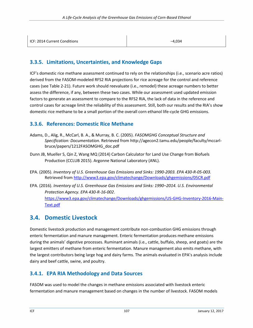
A Life-Cycle Analysis of the Greenhouse Gas Emissions of Corn-Based Ethanol
ICF 107 January 12, 2017
ICF: 2014 Current Conditions −4,034
3.3.5. Limitations, Uncertainties, and Knowledge Gaps
ICF’s domestic rice methane assessment continued to rely on the relationships (i.e., scenario acre ratios)
derived from the FASOM-modeled RFS2 RIA projections for rice acreage for the control and reference
cases (see Table 2-21). Future work should reevaluate (i.e., remodel) these acreage numbers to better
assess the difference, if any, between these two cases. While our assessment used updated emission
factors to generate an assessment to compare to the RFS2 RIA, the lack of data in the reference and
control cases for acreage limit the reliability of this assessment. Still, both our results and the RIA’s show
domestic rice methane to be a small portion of the overall corn ethanol life-cycle GHG emissions.
3.3.6. References: Domestic Rice Methane
Adams, D., Alig, R., McCarl, B. A., & Murray, B. C. (2005). FASOMGHG Conceptual Structure and Specification: Documentation. Retrieved from http://agecon2.tamu.edu/people/faculty/mccarl-bruce/papers/1212FASOMGHG_doc.pdf
Dunn JB, Mueller S, Qin Z, Wang MQ (2014) Carbon Calculator for Land Use Change from Biofuels
Production (CCLUB 2015). Argonne National Laboratory (ANL).
EPA. (2005). Inventory of U.S. Greenhouse Gas Emissions and Sinks: 1990-2003. EPA 430-R-05-003. Retrieved from http://www3.epa.gov/climatechange/Downloads/ghgemissions/05CR.pdf
EPA. (2016). Inventory of U.S. Greenhouse Gas Emissions and Sinks: 1990–2014. U.S. Environmental
Protection Agency. EPA 430-R-16-002.
https://www3.epa.gov/climatechange/Downloads/ghgemissions/US-GHG-Inventory-2016-Main-
Text.pdf
3.4. Domestic Livestock
Domestic livestock production and management contribute non-combustion GHG emissions through
enteric fermentation and manure management. Enteric fermentation produces methane emissions
during the animals’ digestive processes. Ruminant animals (i.e., cattle, buffalo, sheep, and goats) are the
largest emitters of methane from enteric fermentation. Manure management also emits methane, with
the largest contributors being large hog and dairy farms. The animals evaluated in EPA’s analysis include
dairy and beef cattle, swine, and poultry.
3.4.1. EPA RIA Methodology and Data Sources
FASOM was used to model the changes in methane emissions associated with livestock enteric
fermentation and manure management based on changes in the number of livestock. FASOM models
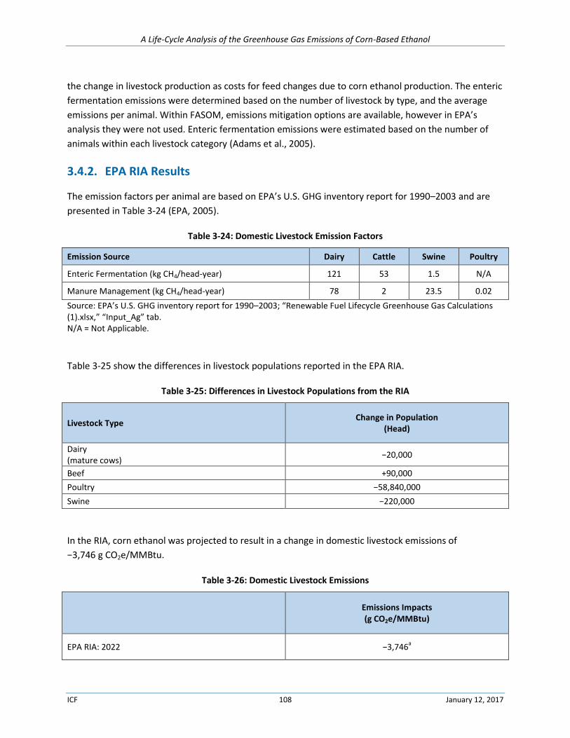
A Life-Cycle Analysis of the Greenhouse Gas Emissions of Corn-Based Ethanol
ICF 108 January 12, 2017
the change in livestock production as costs for feed changes due to corn ethanol production. The enteric
fermentation emissions were determined based on the number of livestock by type, and the average
emissions per animal. Within FASOM, emissions mitigation options are available, however in EPA’s
analysis they were not used. Enteric fermentation emissions were estimated based on the number of
animals within each livestock category (Adams et al., 2005).
3.4.2. EPA RIA Results
The emission factors per animal are based on EPA’s U.S. GHG inventory report for 1990–2003 and are
presented in Table 3-24 (EPA, 2005).
Table 3-24: Domestic Livestock Emission Factors
Emission Source Dairy Cattle Swine Poultry
Enteric Fermentation (kg CH4/head-year) 121 53 1.5 N/A
Manure Management (kg CH4/head-year) 78 2 23.5 0.02
Source: EPA’s U.S. GHG inventory report for 1990–2003; “Renewable Fuel Lifecycle Greenhouse Gas Calculations (1).xlsx,” “Input_Ag” tab. N/A = Not Applicable.
Table 3-25 show the differences in livestock populations reported in the EPA RIA.
Table 3-25: Differences in Livestock Populations from the RIA
Livestock Type Change in Population
(Head)
Dairy (mature cows)
−20,000
Beef +90,000
Poultry
−58,840,000
Swine −220,000
In the RIA, corn ethanol was projected to result in a change in domestic livestock emissions of
−3,746 g CO2e/MMBtu.
Table 3-26: Domestic Livestock Emissions
Emissions Impacts (g CO2e/MMBtu)
EPA RIA: 2022 −3,746a
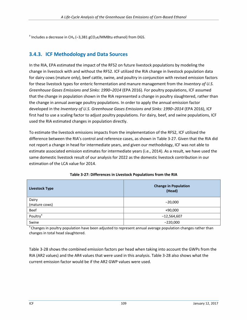
A Life-Cycle Analysis of the Greenhouse Gas Emissions of Corn-Based Ethanol
ICF 109 January 12, 2017
a Includes a decrease in CH4 (−3,381 gCO2e/MMBtu ethanol) from DGS.
3.4.3. ICF Methodology and Data Sources
In the RIA, EPA estimated the impact of the RFS2 on future livestock populations by modeling the
change in livestock with and without the RFS2. ICF utilized the RIA change in livestock population data
for dairy cows (mature only), beef cattle, swine, and poultry in conjunction with revised emission factors
for these livestock types for enteric fermentation and manure management from the Inventory of U.S.
Greenhouse Gases Emissions and Sinks: 1990–2014 (EPA 2016). For poultry populations, ICF assumed
that the change in population shown in the RIA represented a change in poultry slaughtered, rather than
the change in annual average poultry populations. In order to apply the annual emission factor
developed in the Inventory of U.S. Greenhouse Gases Emissions and Sinks: 1990–2014 (EPA 2016), ICF
first had to use a scaling factor to adjust poultry populations. For dairy, beef, and swine populations, ICF
used the RIA estimated changes in population directly.
To estimate the livestock emissions impacts from the implementation of the RFS2, ICF utilized the
difference between the RIA’s control and reference cases, as shown in Table 3-27. Given that the RIA did
not report a change in head for intermediate years, and given our methodology, ICF was not able to
estimate associated emission estimates for intermediate years (i.e., 2014). As a result, we have used the
same domestic livestock result of our analysis for 2022 as the domestic livestock contribution in our
estimation of the LCA value for 2014.
Table 3-27: Differences in Livestock Populations from the RIA
Livestock Type Change in Population
(Head)
Dairy (mature cows)
−20,000
Beef +90,000
Poultrya
−12,564,607
Swine −220,000 a
Changes in poultry population have been adjusted to represent annual average population changes rather than changes in total head slaughtered.
Table 3-28 shows the combined emission factors per head when taking into account the GWPs from the
RIA (AR2 values) and the AR4 values that were used in this analysis. Table 3-28 also shows what the
current emission factor would be if the AR2 GWP values were used.
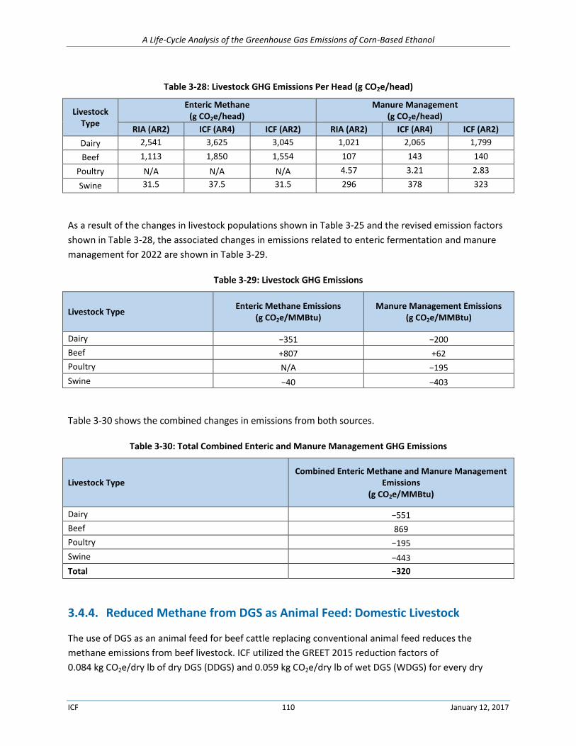
A Life-Cycle Analysis of the Greenhouse Gas Emissions of Corn-Based Ethanol
ICF 110 January 12, 2017
Table 3-28: Livestock GHG Emissions Per Head (g CO2e/head)
Livestock Type
Enteric Methane (g CO2e/head)
Manure Management (g CO2e/head)
RIA (AR2) ICF (AR4) ICF (AR2) RIA (AR2) ICF (AR4) ICF (AR2)
Dairy 2,541 3,625 3,045 1,021 2,065 1,799
Beef 1,113 1,850 1,554 107 143 140
Poultry N/A N/A N/A 4.57 3.21 2.83
Swine 31.5 37.5 31.5 296 378 323
As a result of the changes in livestock populations shown in Table 3-25 and the revised emission factors
shown in Table 3-28, the associated changes in emissions related to enteric fermentation and manure
management for 2022 are shown in Table 3-29.
Table 3-29: Livestock GHG Emissions
Livestock Type Enteric Methane Emissions
(g CO2e/MMBtu) Manure Management Emissions
(g CO2e/MMBtu)
Dairy −351 −200
Beef +807 +62
Poultry N/A −195
Swine −40 −403
Table 3-30 shows the combined changes in emissions from both sources.
Table 3-30: Total Combined Enteric and Manure Management GHG Emissions
Livestock Type Combined Enteric Methane and Manure Management
Emissions (g CO2e/MMBtu)
Dairy −551
Beef 869
Poultry −195
Swine −443
Total −320
3.4.4. Reduced Methane from DGS as Animal Feed: Domestic Livestock
The use of DGS as an animal feed for beef cattle replacing conventional animal feed reduces the
methane emissions from beef livestock. ICF utilized the GREET 2015 reduction factors of
0.084 kg CO2e/dry lb of dry DGS (DDGS) and 0.059 kg CO2e/dry lb of wet DGS (WDGS) for every dry
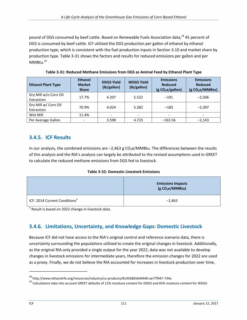
A Life-Cycle Analysis of the Greenhouse Gas Emissions of Corn-Based Ethanol
ICF 111 January 12, 2017
pound of DGS consumed by beef cattle. Based on Renewable Fuels Association data,28 45 percent of
DGS is consumed by beef cattle. ICF utilized the DGS production per gallon of ethanol by ethanol
production type, which is consistent with the fuel production inputs in Section 3.10 and market share by
production type. Table 3-31 shows the factors and results for reduced emissions per gallon and per
MMBtu.29
Table 3-31: Reduced Methane Emissions from DGS as Animal Feed by Ethanol Plant Type
Ethanol Plant Type Ethanol Market Share
DDGS Yield (lb/gallon)
WDGS Yield (lb/gallon)
Emissions Reduced
(g CO2e/gallon)
Emissions Reduced
(g CO2e/MMBtu)
Dry Mill w/o Corn Oil Extraction
17.7% 4.207 5.522 −191 −2,506
Dry Mill w/ Corn Oil Extraction
70.9% 4.024 5.282 −183 −2,397
Wet Mill 11.4% - - - -
Per Average Gallon - 3.598 4.723 −163.56 −2,143
3.4.5. ICF Results
In our analysis, the combined emissions are −2,463 g CO2e/MMBtu. The differences between the results
of this analysis and the RIA’s analysis can largely be attributed to the revised assumptions used in GREET
to calculate the reduced methane emissions from DGS fed to livestock.
Table 3-32: Domestic Livestock Emissions
Emissions Impacts (g CO2e/MMBtu)
ICF: 2014 Current Conditionsa −2,463
a Result is based on 2022 change in livestock data.
3.4.6. Limitations, Uncertainty, and Knowledge Gaps: Domestic Livestock
Because ICF did not have access to the RIA’s original control and reference scenario data, there is
uncertainty surrounding the populations utilized to create the original changes in livestock. Additionally,
as the original RIA only provided a single output for the year 2022, data was not available to develop
changes in livestock emissions for intermediate years, therefore the emission changes for 2022 are used
as a proxy. Finally, we do not believe the RIA accounted for increases in livestock production over time,
28 http://www.ethanolrfa.org/resources/industry/co-products/#1456865649440-ae77f947-734a
29 Calculations take into account GREET defaults of 12% moisture content for DDGS and 65% moisture content for WDGS
A Life-Cycle Analysis of the Greenhouse Gas Emissions of Corn-Based Ethanol
ICF 112 January 12, 2017
e.g., dairy milk production and beef weight increases when accounting for the population changes in
future years. Therefore, the population changes also do not consider these production changes.
The change in poultry populations used in the RIA appears to represent the total number of animals
alive during each year. ICF adjusted this number to represent a steady-state population to account for
the lifetime of the animals. ICF’s adjustment for the number of steady-state heads is more appropriate
for the emission factors used from EPA (2016) which are on an emissions per head per year basis. This
analysis, like the RIA, only takes into account the change in livestock populations between the reference
and control cases.
3.4.7. References: Domestic Livestock
Adams, D., Alig, R., McCarl, B. A., & Murray, B. C. (2005). FASOMGHG Conceptual Structure and Specification: Documentation. Retrieved from http://agecon2.tamu.edu/people/faculty/mccarl-bruce/papers/1212FASOMGHG_doc.pdf
EPA, 2005. Inventory of U.S. Greenhouse Gas Emissions and Sinks: 1990-2003. EPA 430-R-05-003. Retrieved from http://www3.epa.gov/climatechange/Downloads/ghgemissions/05CR.pdf
EPA, 2010a. Renewable Fuel Standard Program (RFS2) Regulatory Impact Analysis. EPA-420-r-10-006. February 2010.
EPA, 2016. Inventory of U.S. Greenhouse Gas Emissions and Sinks: 1990–2014. U.S. Environmental Protection Agency. EPA 430-R-16-002. https://www3.epa.gov/climatechange/Downloads/ghgemissions/US-GHG-Inventory-2016-Main-Text.pdf
USDA, 2016b. USDA Agricultural Projections to 2025. USDA Agricultural Projections No. (OCE-2016-1) 99 pp, February 2016. http://www.ers.usda.gov/publications/oce-usda-agricultural-projections/oce-2016-1.aspx
3.5. International Livestock
In order to be congruous with the domestic livestock emissions, enteric fermentation and manure
management were evaluated for international livestock. The GHG impacts associated with changes in
livestock across seven regions were calculated. The number of livestock was determined for: Canada,
Western Europe, Eastern Europe, Oceania, Latin America, Africa, the Middle East, and India using the
FAPRI-CARD model (FAPRI, 2004). The animals evaluated include dairy and beef cattle, swine, sheep, and
poultry.
3.5.1. EPA RIA Methodology and Data Sources
Based on a similar methodology to the domestic livestock impacts, the FAPRI-CARD model determined
the change in livestock production based on feed prices, and these changes were multiplied by the GHG
emission factors for both enteric fermentation and manure management. The enteric fermentation
emissions were determined based on the number of livestock by type, and the average emissions per
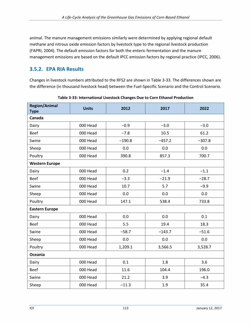
A Life-Cycle Analysis of the Greenhouse Gas Emissions of Corn-Based Ethanol
ICF 113 January 12, 2017
animal. The manure management emissions similarly were determined by applying regional default
methane and nitrous oxide emission factors by livestock type to the regional livestock production
(FAPRI, 2004). The default emission factors for both the enteric fermentation and the manure
management emissions are based on the default IPCC emission factors by regional practice (IPCC, 2006).
3.5.2. EPA RIA Results
Changes in livestock numbers attributed to the RFS2 are shown in Table 3-33. The differences shown are
the difference (in thousand livestock head) between the Fuel-Specific Scenario and the Control Scenario.
Table 3-33: International Livestock Changes Due to Corn Ethanol Production
Region/Animal Type
Units 2012 2017 2022
Canada
Dairy 000 Head −0.9 −3.0 −3.0
Beef 000 Head −7.8 10.5 61.2
Swine 000 Head −190.8 −457.2 −307.8
Sheep 000 Head 0.0 0.0 0.0
Poultry 000 Head 390.8 857.3 700.7
Western Europe
Dairy 000 Head 0.2 −1.4 −1.1
Beef 000 Head −3.3 −21.9 −28.7
Swine 000 Head 10.7 5.7 −9.9
Sheep 000 Head 0.0 0.0 0.0
Poultry 000 Head 147.1 538.4 733.8
Eastern Europe
Dairy 000 Head 0.0 0.0 0.1
Beef 000 Head 5.5 19.4 18.3
Swine 000 Head −58.7 −143.7 −51.6
Sheep 000 Head 0.0 0.0 0.0
Poultry 000 Head 1,209.1 3,566.5 3,528.7
Oceania
Dairy 000 Head 0.1 1.8 3.6
Beef 000 Head 11.6 104.4 196.0
Swine 000 Head 21.2 3.9 −4.3
Sheep 000 Head −11.3 1.9 35.4
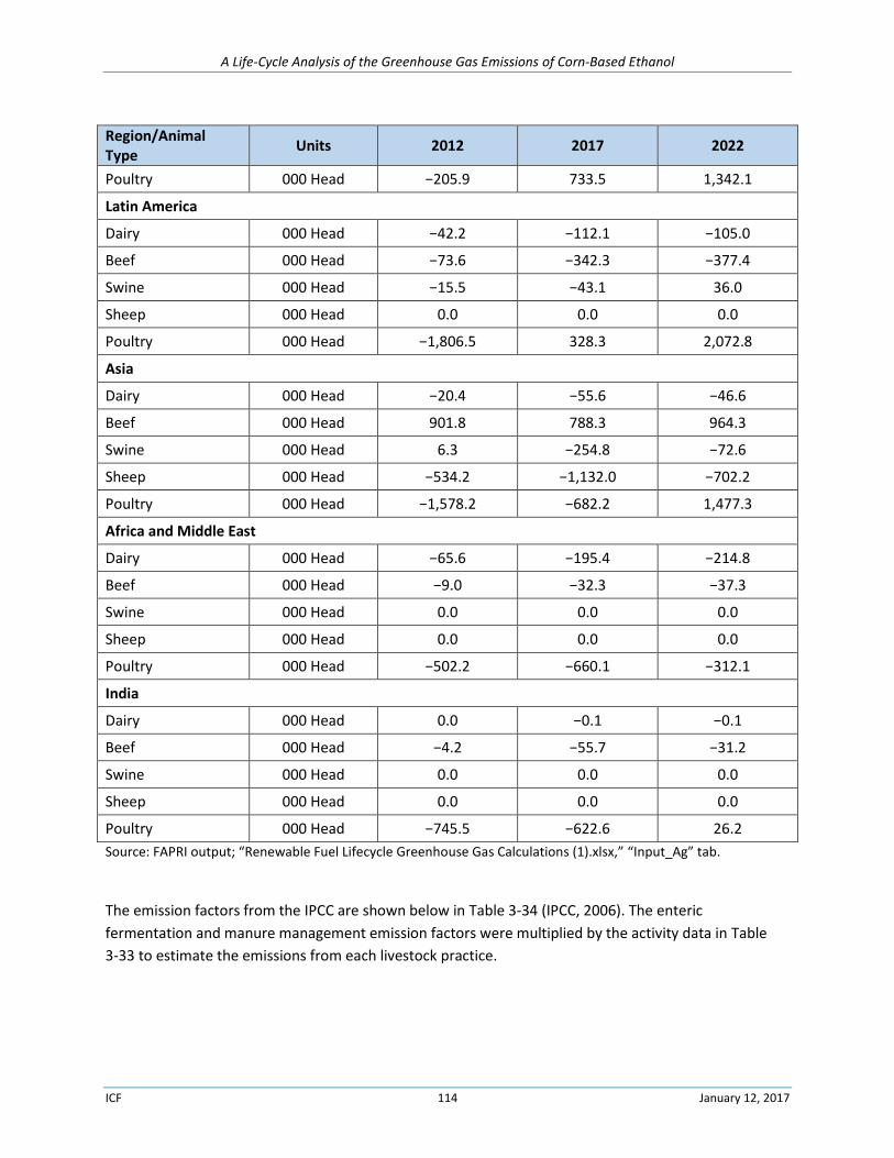
A Life-Cycle Analysis of the Greenhouse Gas Emissions of Corn-Based Ethanol
ICF 114 January 12, 2017
Region/Animal Type
Units 2012 2017 2022
Poultry 000 Head −205.9 733.5 1,342.1
Latin America
Dairy 000 Head −42.2 −112.1 −105.0
Beef 000 Head −73.6 −342.3 −377.4
Swine 000 Head −15.5 −43.1 36.0
Sheep 000 Head 0.0 0.0 0.0
Poultry 000 Head −1,806.5 328.3 2,072.8
Asia
Dairy 000 Head −20.4 −55.6 −46.6
Beef 000 Head 901.8 788.3 964.3
Swine 000 Head 6.3 −254.8 −72.6
Sheep 000 Head −534.2 −1,132.0 −702.2
Poultry 000 Head −1,578.2 −682.2 1,477.3
Africa and Middle East
Dairy 000 Head −65.6 −195.4 −214.8
Beef 000 Head −9.0 −32.3 −37.3
Swine 000 Head 0.0 0.0 0.0
Sheep 000 Head 0.0 0.0 0.0
Poultry 000 Head −502.2 −660.1 −312.1
India
Dairy 000 Head 0.0 −0.1 −0.1
Beef 000 Head −4.2 −55.7 −31.2
Swine 000 Head 0.0 0.0 0.0
Sheep 000 Head 0.0 0.0 0.0
Poultry 000 Head −745.5 −622.6 26.2
Source: FAPRI output; “Renewable Fuel Lifecycle Greenhouse Gas Calculations (1).xlsx,” “Input_Ag” tab.
The emission factors from the IPCC are shown below in Table 3-34 (IPCC, 2006). The enteric
fermentation and manure management emission factors were multiplied by the activity data in Table
3-33 to estimate the emissions from each livestock practice.
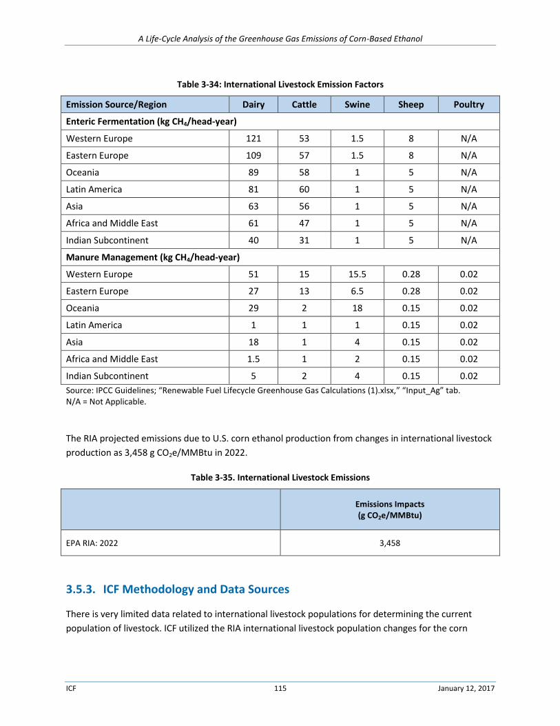
A Life-Cycle Analysis of the Greenhouse Gas Emissions of Corn-Based Ethanol
ICF 115 January 12, 2017
Table 3-34: International Livestock Emission Factors
Emission Source/Region Dairy Cattle Swine Sheep Poultry
Enteric Fermentation (kg CH4/head-year)
Western Europe 121 53 1.5 8 N/A
Eastern Europe 109 57 1.5 8 N/A
Oceania 89 58 1 5 N/A
Latin America 81 60 1 5 N/A
Asia 63 56 1 5 N/A
Africa and Middle East 61 47 1 5 N/A
Indian Subcontinent 40 31 1 5 N/A
Manure Management (kg CH4/head-year)
Western Europe 51 15 15.5 0.28 0.02
Eastern Europe 27 13 6.5 0.28 0.02
Oceania 29 2 18 0.15 0.02
Latin America 1 1 1 0.15 0.02
Asia 18 1 4 0.15 0.02
Africa and Middle East 1.5 1 2 0.15 0.02
Indian Subcontinent 5 2 4 0.15 0.02
Source: IPCC Guidelines; “Renewable Fuel Lifecycle Greenhouse Gas Calculations (1).xlsx,” “Input_Ag” tab. N/A = Not Applicable.
The RIA projected emissions due to U.S. corn ethanol production from changes in international livestock
production as 3,458 g CO2e/MMBtu in 2022.
Table 3-35. International Livestock Emissions
Emissions Impacts (g CO2e/MMBtu)
EPA RIA: 2022 3,458
3.5.3. ICF Methodology and Data Sources
There is very limited data related to international livestock populations for determining the current
population of livestock. ICF utilized the RIA international livestock population changes for the corn
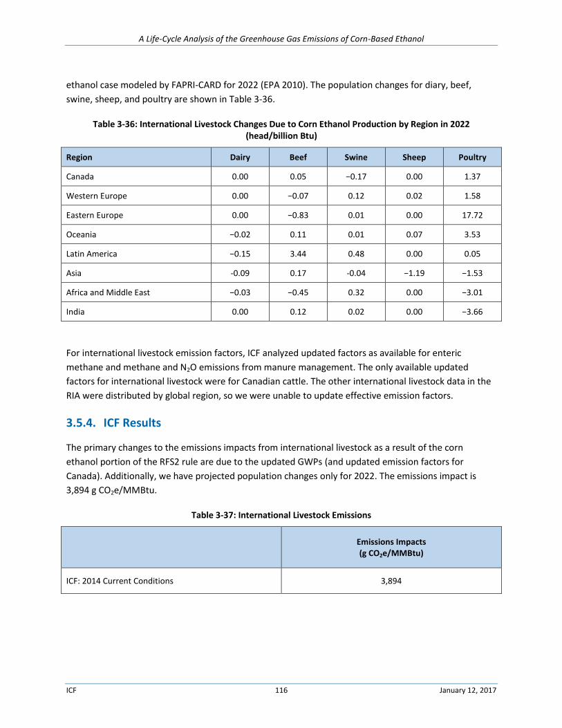
A Life-Cycle Analysis of the Greenhouse Gas Emissions of Corn-Based Ethanol
ICF 116 January 12, 2017
ethanol case modeled by FAPRI-CARD for 2022 (EPA 2010). The population changes for diary, beef,
swine, sheep, and poultry are shown in Table 3-36.
Table 3-36: International Livestock Changes Due to Corn Ethanol Production by Region in 2022 (head/billion Btu)
Region Dairy Beef Swine Sheep Poultry
Canada 0.00 0.05 −0.17 0.00 1.37
Western Europe 0.00 −0.07 0.12 0.02 1.58
Eastern Europe 0.00 −0.83 0.01 0.00 17.72
Oceania −0.02 0.11 0.01 0.07 3.53
Latin America −0.15 3.44 0.48 0.00 0.05
Asia -0.09 0.17 -0.04 −1.19 −1.53
Africa and Middle East −0.03 −0.45 0.32 0.00 −3.01
India 0.00 0.12 0.02 0.00 −3.66
For international livestock emission factors, ICF analyzed updated factors as available for enteric
methane and methane and N2O emissions from manure management. The only available updated
factors for international livestock were for Canadian cattle. The other international livestock data in the
RIA were distributed by global region, so we were unable to update effective emission factors.
3.5.4. ICF Results
The primary changes to the emissions impacts from international livestock as a result of the corn
ethanol portion of the RFS2 rule are due to the updated GWPs (and updated emission factors for
Canada). Additionally, we have projected population changes only for 2022. The emissions impact is
3,894 g CO2e/MMBtu.
Table 3-37: International Livestock Emissions
Emissions Impacts (g CO2e/MMBtu)
ICF: 2014 Current Conditions 3,894
A Life-Cycle Analysis of the Greenhouse Gas Emissions of Corn-Based Ethanol
ICF 117 January 12, 2017
3.5.5. References: International Livestock
EPA, 2010a. Renewable Fuel Standard Program (RFS2) Regulatory Impact Analysis. EPA-420-r-10-006. February 2010.
EPA, 2016. Inventory of U.S. Greenhouse Gas Emissions and Sinks: 1990–2014. U.S. Environmental Protection Agency. EPA 430-R-16-002. https://www3.epa.gov/climatechange/Downloads/ghgemissions/US-GHG-Inventory-2016-Main-Text.pdf
FAPRI. (2004). Documentation the FAPRI Modeling System. Ames, IA: Iowa State University.
IPCC. (2006). 2006 IPCC Guidelines for National Greenhouse Gas Inventories, Prepared by the National Greenhouse Gas Inventories Programme, Eggleston H.S., Buendia L., Miwa K., Ngara T. and. Japan: IGES.
USDA, 2016. USDA Agricultural Projections to 2025. USDA Agricultural Projections No. (OCE-2016-1) 99 pp, February 2016. http://www.ers.usda.gov/publications/oce-usda-agricultural-projections/oce-2016-1.aspx
3.6. International Land-Use Change
To model the change in cropland land internationally in response to increased corn ethanol production
in the United States, the RFS2 RIA used the integrated Food and Agricultural Policy and Research
Institute International model, maintained by the Center for Agricultural and Rural Development at Iowa
State University (FAPRI-CARD) (FAPRI, 2004). 30 The Center for Agricultural and Rural Development at
Iowa State University ran the FAPRI-CARD model on behalf of EPA.
3.6.1. EPA RIA Methodology and Data Sources
FAPRI-CARD projected the total changes in land area used for commodity production (crops and
livestock) cropland by region. The land-cover types (forests, grassland, etc.) affected and the location of
the land conversions were determined using MODIS satellite data provided by Winrock International
who produces the land-use conversions internationally from 2001 to 2007 (MODIS; Friedl, 2009). The
land conversion scenarios analyzed were the following:
Annual Crops to/from Perennial Crops
Pasture to/from Perennial Crops
Pasture to/from Annual Crops
Natural Ecosystems to/from Annual Crops
Natural Ecosystems to/from Perennial Crops
30 The Farm and Agricultural Policy Research Institute’s FAPRI CARD model examines and projects the production, use, stocks,
prices, and trade for ethanol for several countries and regions of the world.
A Life-Cycle Analysis of the Greenhouse Gas Emissions of Corn-Based Ethanol
ICF 118 January 12, 2017
Natural Ecosystems to/from Pasture
Natural ecosystems include forests, grasslands, savannas, shrublands, wetlands, and barren land.
The assessment assumes that the social, political, and economic forces that drove land-use change
during this period of time will remain the same through 2022.
The international land-use change emission impacts are based on:
Land Conversion Categories: The different types of land conversions were analyzed with satellite
data to show their location and the land-cover types affected in order to estimate the international
land-use change.
Forest Carbon Stock Estimates: EPA’s emission factors incorporated spatial, region-specific maps
derived using adjusted biome-level Tier 1 default values from IPCC and supplemented with country-
specific data sources (Ruesch and Gibbs, 2008).
Land Clearing with Fire: Fire for land clearing is assumed to occur in all countries included in the
analysis except China and Argentina. These estimates are based on the area burnt, the mass of fuel
used for combustion and the emission factor for dry matter (IPCC, 2006).
Changes in Soil Carbon Stocks: The changes in soil carbon stocks on land converted to cropland
were calculated based on Section 5.3.3.4 of the IPCC AFOLU section. The specific soil stock change
factors used for land use, management, and inputs were multiplied by the reference carbon stocks.
Following IPCC guidelines, the total difference in carbon stocks before and after conversion was
averaged over 20 years (IPCC, 2006).
Foregone Forest Sequestration: Forest sequestration rates were taken from the IPCC Tier 1 default
values for native forests. Updated literature values were available for tropical intact old growth
forests (0.49 t C/ha/yr) and temperate and boreal forests (3–4 t CO2e/ha/yr) (Lewis et al., 2009)
(Myneni et al., 2001).
Land Reversion Carbon Uptake Factors: All reversion factors (except reversion to forest) were
estimated as the reverse of emission factors, and all increases in biomass stocks occurred in Year 1.
Forest reversion factors are based on the assumption that biomass accumulates every year over the
entire 30-year time period.
Change in Pasture Land Conversion: The analysis accounted for changes in pasture area resulting
from livestock fluctuations in order to create a link between the livestock and land used for grazing.
The regional pasture stocking rates determine the amount of land needed for pasture. Any
unneeded pasture areas are available for cropland or to be returned to their natural state. In
countries where the livestock rates increased, the land used for pasture can be added to the
abandoned cropland, unused grassland, or result in deforestation. The average stocking rates for
each of the 54 FAPRI-CARD regions were determined based on data on livestock populations from
the United Nations Food and Agricultural Organization (FAO) (see Table 2.4-31 from EPA RIA) (EPA,
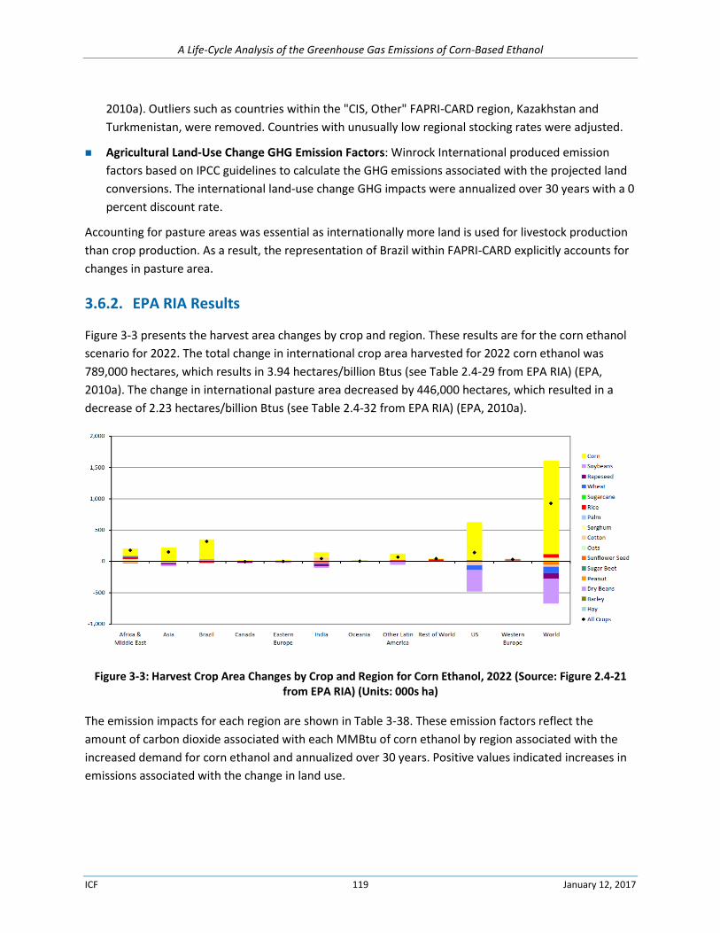
A Life-Cycle Analysis of the Greenhouse Gas Emissions of Corn-Based Ethanol
ICF 119 January 12, 2017
2010a). Outliers such as countries within the "CIS, Other" FAPRI-CARD region, Kazakhstan and
Turkmenistan, were removed. Countries with unusually low regional stocking rates were adjusted.
Agricultural Land-Use Change GHG Emission Factors: Winrock International produced emission
factors based on IPCC guidelines to calculate the GHG emissions associated with the projected land
conversions. The international land-use change GHG impacts were annualized over 30 years with a 0
percent discount rate.
Accounting for pasture areas was essential as internationally more land is used for livestock production
than crop production. As a result, the representation of Brazil within FAPRI-CARD explicitly accounts for
changes in pasture area.
3.6.2. EPA RIA Results
Figure 3-3 presents the harvest area changes by crop and region. These results are for the corn ethanol
scenario for 2022. The total change in international crop area harvested for 2022 corn ethanol was
789,000 hectares, which results in 3.94 hectares/billion Btus (see Table 2.4-29 from EPA RIA) (EPA,
2010a). The change in international pasture area decreased by 446,000 hectares, which resulted in a
decrease of 2.23 hectares/billion Btus (see Table 2.4-32 from EPA RIA) (EPA, 2010a).
Figure 3-3: Harvest Crop Area Changes by Crop and Region for Corn Ethanol, 2022 (Source: Figure 2.4-21 from EPA RIA) (Units: 000s ha)
The emission impacts for each region are shown in Table 3-38. These emission factors reflect the
amount of carbon dioxide associated with each MMBtu of corn ethanol by region associated with the
increased demand for corn ethanol and annualized over 30 years. Positive values indicated increases in
emissions associated with the change in land use.
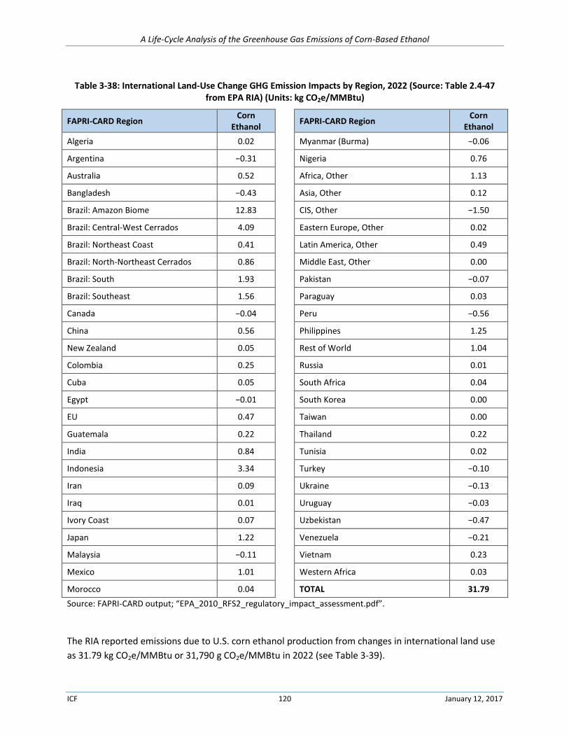
A Life-Cycle Analysis of the Greenhouse Gas Emissions of Corn-Based Ethanol
ICF 120 January 12, 2017
Table 3-38: International Land-Use Change GHG Emission Impacts by Region, 2022 (Source: Table 2.4-47 from EPA RIA) (Units: kg CO2e/MMBtu)
FAPRI-CARD Region Corn
Ethanol FAPRI-CARD Region
Corn Ethanol
Algeria 0.02 Myanmar (Burma) −0.06
Argentina −0.31 Nigeria 0.76
Australia 0.52 Africa, Other 1.13
Bangladesh −0.43 Asia, Other 0.12
Brazil: Amazon Biome 12.83 CIS, Other −1.50
Brazil: Central-West Cerrados 4.09 Eastern Europe, Other 0.02
Brazil: Northeast Coast 0.41 Latin America, Other 0.49
Brazil: North-Northeast Cerrados 0.86 Middle East, Other 0.00
Brazil: South 1.93 Pakistan −0.07
Brazil: Southeast 1.56 Paraguay 0.03
Canada −0.04 Peru −0.56
China 0.56 Philippines 1.25
New Zealand 0.05 Rest of World 1.04
Colombia 0.25 Russia 0.01
Cuba 0.05 South Africa 0.04
Egypt −0.01 South Korea 0.00
EU 0.47 Taiwan 0.00
Guatemala 0.22 Thailand 0.22
India 0.84 Tunisia 0.02
Indonesia 3.34 Turkey −0.10
Iran 0.09 Ukraine −0.13
Iraq 0.01 Uruguay −0.03
Ivory Coast 0.07 Uzbekistan −0.47
Japan 1.22 Venezuela −0.21
Malaysia −0.11 Vietnam 0.23
Mexico 1.01 Western Africa 0.03
Morocco 0.04 TOTAL 31.79
Source: FAPRI-CARD output; “EPA_2010_RFS2_regulatory_impact_assessment.pdf”.
The RIA reported emissions due to U.S. corn ethanol production from changes in international land use
as 31.79 kg CO2e/MMBtu or 31,790 g CO2e/MMBtu in 2022 (see Table 3-39).
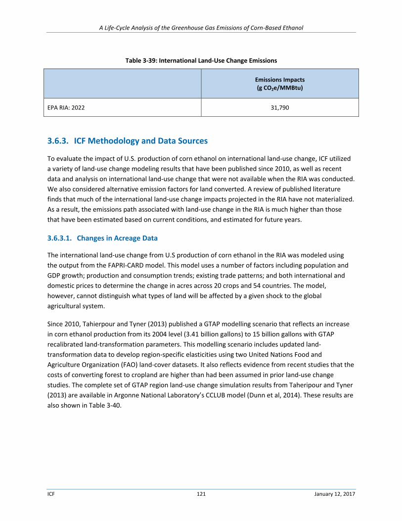
A Life-Cycle Analysis of the Greenhouse Gas Emissions of Corn-Based Ethanol
ICF 121 January 12, 2017
Table 3-39: International Land-Use Change Emissions
Emissions Impacts (g CO2e/MMBtu)
EPA RIA: 2022 31,790
3.6.3. ICF Methodology and Data Sources
To evaluate the impact of U.S. production of corn ethanol on international land-use change, ICF utilized
a variety of land-use change modeling results that have been published since 2010, as well as recent
data and analysis on international land-use change that were not available when the RIA was conducted.
We also considered alternative emission factors for land converted. A review of published literature
finds that much of the international land-use change impacts projected in the RIA have not materialized.
As a result, the emissions path associated with land-use change in the RIA is much higher than those
that have been estimated based on current conditions, and estimated for future years.
3.6.3.1. Changes in Acreage Data
The international land-use change from U.S production of corn ethanol in the RIA was modeled using
the output from the FAPRI-CARD model. This model uses a number of factors including population and
GDP growth; production and consumption trends; existing trade patterns; and both international and
domestic prices to determine the change in acres across 20 crops and 54 countries. The model,
however, cannot distinguish what types of land will be affected by a given shock to the global
agricultural system.
Since 2010, Tahierpour and Tyner (2013) published a GTAP modelling scenario that reflects an increase
in corn ethanol production from its 2004 level (3.41 billion gallons) to 15 billion gallons with GTAP
recalibrated land-transformation parameters. This modelling scenario includes updated land-
transformation data to develop region-specific elasticities using two United Nations Food and
Agriculture Organization (FAO) land-cover datasets. It also reflects evidence from recent studies that the
costs of converting forest to cropland are higher than had been assumed in prior land-use change
studies. The complete set of GTAP region land-use change simulation results from Taheripour and Tyner
(2013) are available in Argonne National Laboratory’s CCLUB model (Dunn et al, 2014). These results are
also shown in Table 3-40.
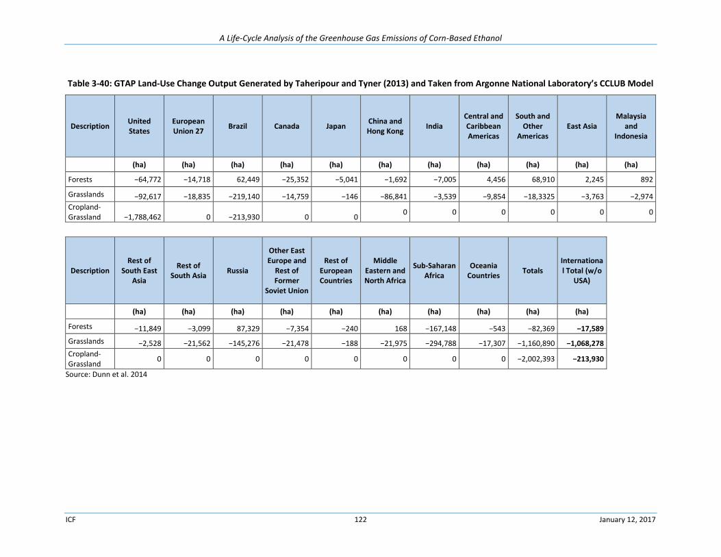
A Life-Cycle Analysis of the Greenhouse Gas Emissions of Corn-Based Ethanol
ICF 122 January 12, 2017
Table 3-40: GTAP Land-Use Change Output Generated by Taheripour and Tyner (2013) and Taken from Argonne National Laboratory’s CCLUB Model
Description United States
European Union 27
Brazil Canada Japan China and Hong Kong
India Central and Caribbean Americas
South and Other
Americas East Asia
Malaysia and
Indonesia
(ha) (ha) (ha) (ha) (ha) (ha) (ha) (ha) (ha) (ha) (ha)
Forests −64,772 −14,718 62,449 −25,352 −5,041 −1,692 −7,005 4,456 68,910 2,245 892
Grasslands −92,617 −18,835 −219,140 −14,759 −146 −86,841 −3,539 −9,854 −18,3325 −3,763 −2,974
Cropland-Grassland −1,788,462 0 −213,930 0 0
0 0 0 0 0 0
Description Rest of
South East Asia
Rest of South Asia
Russia
Other East Europe and
Rest of Former
Soviet Union
Rest of European Countries
Middle Eastern and North Africa
Sub-Saharan Africa
Oceania Countries
Totals International Total (w/o
USA)
(ha) (ha) (ha) (ha) (ha) (ha) (ha) (ha) (ha) (ha)
Forests −11,849 −3,099 87,329 −7,354 −240 168 −167,148 −543 −82,369 −17,589 Grasslands −2,528 −21,562 −145,276 −21,478 −188 −21,975 −294,788 −17,307 −1,160,890 −1,068,278 Cropland-
Grassland 0 0 0 0 0 0 0 0 −2,002,393 −213,930
Source: Dunn et al. 2014
A Life-Cycle Analysis of the Greenhouse Gas Emissions of Corn-Based Ethanol
ICF 123 January 12, 2017
Since 2010, a number of studies have evaluated the land-use change outcomes projected in the RIA (see
Chapter 2). These studies generally conclude that there is not a strong link between corn ethanol
production in the United States and deforestation in other countries, particularly in Brazil where much
of the RIA’s emissions related to indirect land use change were projected to occur. Additionally, among
the broad range of emission estimates associated with indirect land-use change, across studies these
estimates have decreased over time. For the land-use change that has been observed, Bruce Babcock
and Zabid Iqbal’s publication “Using Recent Land Use Changes to Validate Land Use Change Models”
confirmed that the primary response from farmers across the world during the period 2004–2012 was to
use available land resources more efficiently rather than to expand the amount of land in production.
Farmers in Brazil, India, and China have increased double cropping, reduced unharvested planted area,
reduced fallow land, and reduced temporary pasture which explains why the land-use changes
projected in the RIA for Brazil and elsewhere have not materialized (Babcock and Iqbal, 2014).
To develop an updated picture of regional land-use changes that have occurred since 2010 as a result of
increases in corn ethanol production in the United States, ICF incorporated qualitative data from
Babcock and Iqbal (2014) along with recent GTAP simulation results from Dunn et al. 2014. The acres
adjustments relied on one source in order to be consistent across regions.
ICF identified five regions for adjustments based on observed land practices and FAO data analysis.
Brazil: Babcock and Iqbal (2014) show that 76 percent of Brazil’s change in acres was due to double
cropped land. This analysis assumes that the 76 percent change can be applied the acreage within
the GTAP output that was attributed to U.S. corn demand.
India: Babcock and Iqbal (2014) note that 100 percent of India’s change in acres should be
attributed to double cropping leading ICF to adjust GTAP 2013 change in acres to zero.
China: Between 2010 and 2012, Babcock and Iqbal (2014) state that 29 percent of China’s change in
harvested acres should be attributed to double cropping. ICF adjusted the GTAP 2013 output to
attribute 71 percent of the country’s change in acres to U.S. corn demand.
Sub-Saharan Africa: According to Babcock and Iqbal (2014), much of region’s crop production was
conducted by small-scale producers without modern farming equipment leading to the idea that
double cropping is not widely adopted. The authors note that given domestic food demand from
growing populations in the region, the extensive land-use increase equaled 20.7 million hectares or
1.35 percent (Babcock and Iqbal 2014). ICF adjusted the GTAP Sub-Saharan Africa region to
allocate 1.35 percent of the GTAP 2013 change in acres to corn ethanol.
Indonesia: Babcock and Iqbal (2014) cite multiple studies that state that the land-use change in
Indonesia attributed to corn production is most likely inflated due to the prevalence of double
cropping and the significant expansion of palm oil production. They commented that a significant
portion of the corn production increase is due to double cropping (Babcock and Iqbal 2014). ICF
attributed 50 percent of the GTAP 2013 acres to those due to corn ethanol demands.
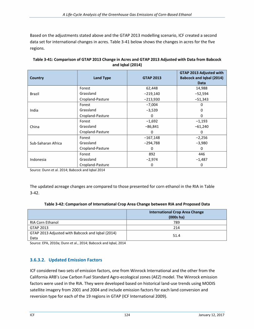
A Life-Cycle Analysis of the Greenhouse Gas Emissions of Corn-Based Ethanol
ICF 124 January 12, 2017
Based on the adjustments stated above and the GTAP 2013 modelling scenario, ICF created a second
data set for international changes in acres. Table 3-41 below shows the changes in acres for the five
regions.
Table 3-41: Comparison of GTAP 2013 Change in Acres and GTAP 2013 Adjusted with Data from Babcock and Iqbal (2014)
Country Land Type GTAP 2013 GTAP 2013 Adjusted with Babcock and Iqbal (2014)
Data
Brazil
Forest 62,448 14,988
Grassland −219,140 −52,594
Cropland-Pasture −213,930 −51,343
India
Forest −7,004 0
Grassland −3,539 0
Cropland-Pasture 0 0
China
Forest −1,692 −1,193
Grassland −86,841 −61,240
Cropland-Pasture 0 0
Sub-Saharan Africa
Forest −167,148 −2,256
Grassland −294,788 −3,980
Cropland-Pasture 0 0
Indonesia
Forest 892 446
Grassland −2,974 −1,487
Cropland-Pasture 0 0 Source: Dunn et al. 2014; Babcock and Iqbal 2014
The updated acreage changes are compared to those presented for corn ethanol in the RIA in Table
3-42.
Table 3-42: Comparison of International Crop Area Change between RIA and Proposed Data
International Crop Area Change
(000s ha)
RIA Corn Ethanol 789
GTAP 2013 214
GTAP 2013 Adjusted with Babcock and Iqbal (2014) Data
51.4
Source: EPA, 2010a; Dunn et al., 2014; Babcock and Iqbal, 2014
3.6.3.2. Updated Emission Factors
ICF considered two sets of emission factors, one from Winrock International and the other from the
California ARB’s Low Carbon Fuel Standard Agro-ecological zones (AEZ) model. The Winrock emission
factors were used in the RIA. They were developed based on historical land-use trends using MODIS
satellite imagery from 2001 and 2004 and include emission factors for each land conversion and
reversion type for each of the 19 regions in GTAP (ICF International 2009).
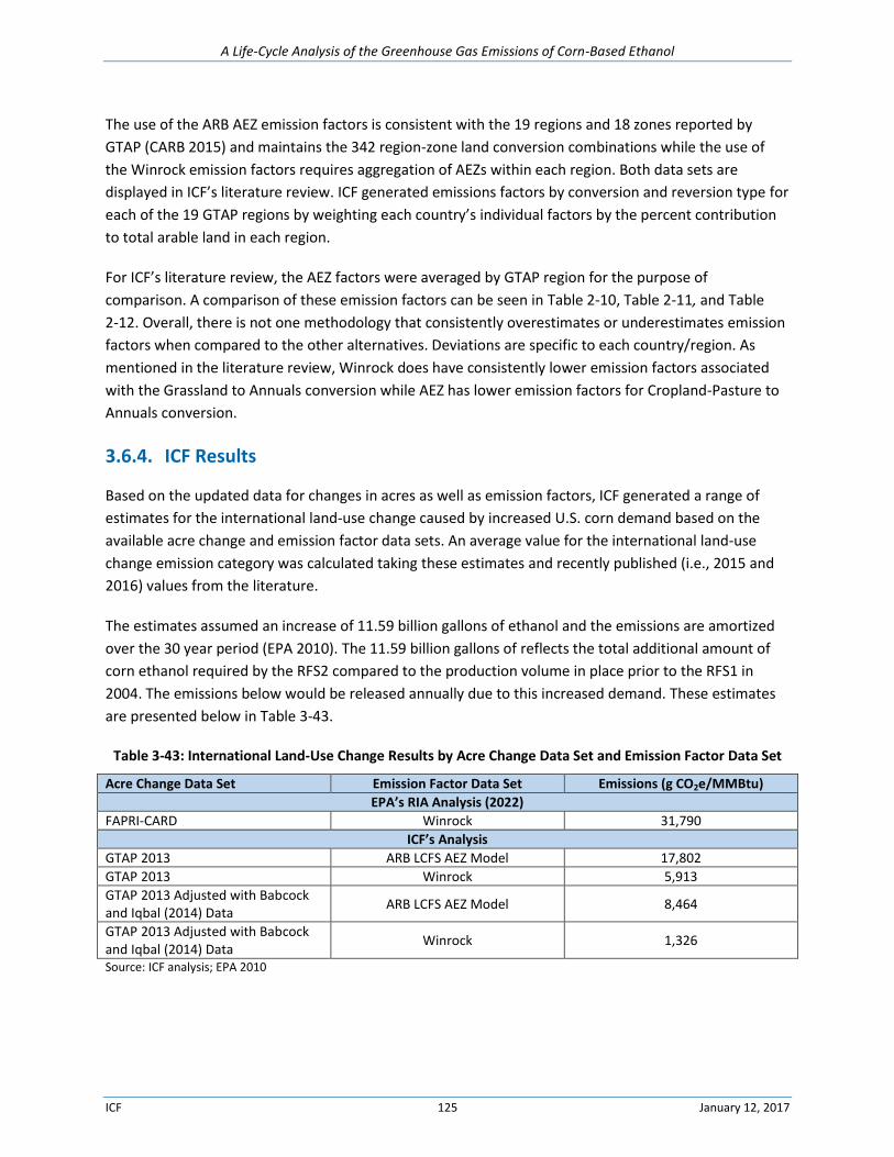
A Life-Cycle Analysis of the Greenhouse Gas Emissions of Corn-Based Ethanol
ICF 125 January 12, 2017
The use of the ARB AEZ emission factors is consistent with the 19 regions and 18 zones reported by
GTAP (CARB 2015) and maintains the 342 region-zone land conversion combinations while the use of
the Winrock emission factors requires aggregation of AEZs within each region. Both data sets are
displayed in ICF’s literature review. ICF generated emissions factors by conversion and reversion type for
each of the 19 GTAP regions by weighting each country’s individual factors by the percent contribution
to total arable land in each region.
For ICF’s literature review, the AEZ factors were averaged by GTAP region for the purpose of
comparison. A comparison of these emission factors can be seen in Table 2-10, Table 2-11, and Table
2-12. Overall, there is not one methodology that consistently overestimates or underestimates emission
factors when compared to the other alternatives. Deviations are specific to each country/region. As
mentioned in the literature review, Winrock does have consistently lower emission factors associated
with the Grassland to Annuals conversion while AEZ has lower emission factors for Cropland-Pasture to
Annuals conversion.
3.6.4. ICF Results
Based on the updated data for changes in acres as well as emission factors, ICF generated a range of
estimates for the international land-use change caused by increased U.S. corn demand based on the
available acre change and emission factor data sets. An average value for the international land-use
change emission category was calculated taking these estimates and recently published (i.e., 2015 and
2016) values from the literature.
The estimates assumed an increase of 11.59 billion gallons of ethanol and the emissions are amortized
over the 30 year period (EPA 2010). The 11.59 billion gallons of reflects the total additional amount of
corn ethanol required by the RFS2 compared to the production volume in place prior to the RFS1 in
2004. The emissions below would be released annually due to this increased demand. These estimates
are presented below in Table 3-43.
Table 3-43: International Land-Use Change Results by Acre Change Data Set and Emission Factor Data Set
Acre Change Data Set Emission Factor Data Set Emissions (g CO2e/MMBtu)
EPA’s RIA Analysis (2022)
FAPRI-CARD Winrock 31,790
ICF’s Analysis
GTAP 2013 ARB LCFS AEZ Model 17,802
GTAP 2013 Winrock 5,913
GTAP 2013 Adjusted with Babcock and Iqbal (2014) Data
ARB LCFS AEZ Model 8,464
GTAP 2013 Adjusted with Babcock and Iqbal (2014) Data
Winrock 1,326
Source: ICF analysis; EPA 2010
A Life-Cycle Analysis of the Greenhouse Gas Emissions of Corn-Based Ethanol
ICF 126 January 12, 2017
All emission calculations presented above are lower that EPA’s RIA estimate of the impacts from
international land-use change.
In regards to acreage data, the GTAP 2013 modelling scenario is more conservative than the GTAP 2013
adjusted with Babcock and Iqbal (2014) data. Although the quantitative analysis conducted by Babcock
and Iqbal (2014) attempts to better represent the actual acreage change for the five regions due to corn
ethanol production, the evidence is not strong enough to solely recommend the qualitative adjustments
that were made. The GTAP 2013 adjusted with Babcock and Iqbal (2014) data with Winrock emission
factors scenario provides the lower bound for this estimate and illustrates that increased corn ethanol
demand could have only a small impact on international land-use change.
The ARB LCFS AEZ does have higher emissions impact estimates than the Winrock data. This analysis is in
line with what was observed during the literature review, where it was determined (see Section 2.2)
that ARB LCFS AEZ would provide the highest emission estimates. These values provide the upper bound
for this analysis.
To reflect the full range of recently published literature relating to the contribution of international land-
use change to the current GHG profile of corn ethanol, ICF adopted a composite approach that averaged
the results of three recently published studies (CARB, 2015; Dunn et al., 2015; and GTAP, 2013) and four
scenarios developed from their results that allow for alternative sets of emissions factors and the
increased use of double cropping (Babcock and Iqbal, 2014). These seven results are shown in Figure 3-4.
Dunn et al. (2015) quantify two emissions related to international land-use change distinguished by the
use of the Winrock and the Woods Hole emissions factors (EFs). ICF developed four scenarios from the
results of the most recently published GTAP study (GTAP 2013) to account for the use of ARB EFs and
Winrock EFs as well as increased double cropping (denoted “Adjusted” in Figure 3-4). Across these seven
results, the average emissions impact is 8.61 g CO2e/MJ. This value converts to 9,082 g CO2e/MMBtu,
which is the value ICF used as the contribution of international land-use change to corn ethanol’s
current GHG profile (see Table 3-44).
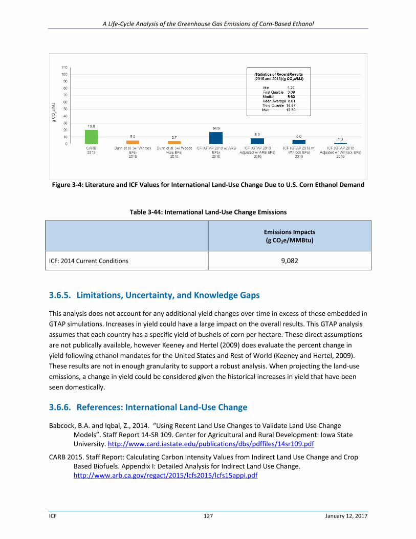
A Life-Cycle Analysis of the Greenhouse Gas Emissions of Corn-Based Ethanol
ICF 127 January 12, 2017
Figure 3-4: Literature and ICF Values for International Land-Use Change Due to U.S. Corn Ethanol Demand
Table 3-44: International Land-Use Change Emissions
Emissions Impacts (g CO2e/MMBtu)
ICF: 2014 Current Conditions 9,082
3.6.5. Limitations, Uncertainty, and Knowledge Gaps
This analysis does not account for any additional yield changes over time in excess of those embedded in
GTAP simulations. Increases in yield could have a large impact on the overall results. This GTAP analysis
assumes that each country has a specific yield of bushels of corn per hectare. These direct assumptions
are not publically available, however Keeney and Hertel (2009) does evaluate the percent change in
yield following ethanol mandates for the United States and Rest of World (Keeney and Hertel, 2009).
These results are not in enough granularity to support a robust analysis. When projecting the land-use
emissions, a change in yield could be considered given the historical increases in yield that have been
seen domestically.
3.6.6. References: International Land-Use Change
Babcock, B.A. and Iqbal, Z., 2014. “Using Recent Land Use Changes to Validate Land Use Change Models”. Staff Report 14-SR 109. Center for Agricultural and Rural Development: Iowa State University. http://www.card.iastate.edu/publications/dbs/pdffiles/14sr109.pdf
CARB 2015. Staff Report: Calculating Carbon Intensity Values from Indirect Land Use Change and Crop Based Biofuels. Appendix I: Detailed Analysis for Indirect Land Use Change. http://www.arb.ca.gov/regact/2015/lcfs2015/lcfs15appi.pdf
A Life-Cycle Analysis of the Greenhouse Gas Emissions of Corn-Based Ethanol
ICF 128 January 12, 2017
Dunn JB, Qin Z, Mueller S, Kwon H, Wander M, Wang M (2014) Carbon Calculator for Land Use Change from Biofuels Production (CCLUB), Users' Manual and Technical Documentation (No. ANL/ESD/12-5 Rev. 2). Argonne National Laboratory (ANL). Available at: https://greet.es.anl.gov/publications.
EPA, 2010a. Renewable Fuel Standard Program (RFS2) Regulatory Impact Analysis. EPA-420-r-10-006. February 2010.
FAPRI. (2004). Documentation the FAPRI Modeling System. Ames, IA: Iowa State University.
Friedl, M. (2009, December). Validation of the Consistent-Year V003 MODIS Land Cover Product, MODIS Land Team Internal PI Document. Retrieved from http://landval.gsfc.nasa.gov/Results.php?TitleID=mod12_valsup1
ICF International, 2009. Emissions from Land Use Change due to Increased Biofuel Production. Satellite Imagery and Emissions Factor Analysis. Peer Review Report.
IPCC. (2006). 2006 IPCC Guidelines for National Greenhouse Gas Inventories, Prepared by the National Greenhouse Gas Inventories Programme, Eggleston H.S., Buendia L., Miwa K., Ngara T. and. Japan: IGES.
Keeney, R. and Hertel, T.W. 2009. “The Indirect Land Use Impacts Of United States Biofuels Policies: The Importance Of Acreage, Yield, And Bilateral Trade Responses”. American Journal of Agricultural Economics. 91(4). 895-909. http://web.ics.purdue.edu/~hertel/data/uploads/publications/keeney-hertel-ajae.pdf
Lewis, S.L., G. Lopez-Gonzalez, B. Sonké, K. Affum Bafoe, T.R. Baker, L.O. Ojo, O.L. (2009). Increasing carbon storage in intact African tropical forests. Nature, 1003-1006.
MODIS. (n.d.). MODIS/Terra Land Cover Type Yearly L3 Global 1km SIN GRID (MOD12Q1) Version 4.
Myneni, R.B., D. Jong, C.J. Tucker, R.K. Kaufmann, P.E. Kauppi, J. Liski, L. Zhou, V. (2001). A large carbon sink in the woody biomass of Northern forests. PNAS, 14784-14789.
Ruesch, A. and H.K. Gibbs. (2008). New IPCC Tier-1 Global Biomass Carbon Map For the. Retrieved from Oak Ridge National Laboratory: http://cdiac.ornl.gov
Taheripour F., Tyner W.E., 2013. Biofuels and land use change: Applying recent evidence to model estimates. Applied Sciences, 3, 14–38.
3.7. International Farm Inputs and Fertilizer N2O
The international farm inputs included in the RFS2 analysis include fertilizers, herbicides, pesticides,
energy use, and direct and indirect fertilizer N2O emissions.
3.7.1. EPA RIA Methodology and Data Sources
The activity data for international farm inputs are based on the following methods and sources:
Fertilizer Application Rates: The changes in crop area and production by crop type and country
output from the FAPRI-CARD model was used to determine the applied amount of fertilizer.
Regional fertilizer application rates (kg/ha) were taken from the International Fertilizer Industry
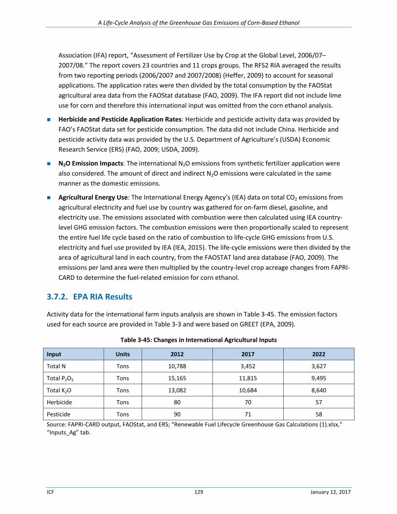
A Life-Cycle Analysis of the Greenhouse Gas Emissions of Corn-Based Ethanol
ICF 129 January 12, 2017
Association (IFA) report, “Assessment of Fertilizer Use by Crop at the Global Level, 2006/07–
2007/08.” The report covers 23 countries and 11 crops groups. The RFS2 RIA averaged the results
from two reporting periods (2006/2007 and 2007/2008) (Heffer, 2009) to account for seasonal
applications. The application rates were then divided by the total consumption by the FAOStat
agricultural area data from the FAOStat database (FAO, 2009). The IFA report did not include lime
use for corn and therefore this international input was omitted from the corn ethanol analysis.
Herbicide and Pesticide Application Rates: Herbicide and pesticide activity data was provided by
FAO’s FAOStat data set for pesticide consumption. The data did not include China. Herbicide and
pesticide activity data was provided by the U.S. Department of Agriculture’s (USDA) Economic
Research Service (ERS) (FAO, 2009; USDA, 2009).
N2O Emission Impacts: The international N2O emissions from synthetic fertilizer application were
also considered. The amount of direct and indirect N2O emissions were calculated in the same
manner as the domestic emissions.
Agricultural Energy Use: The International Energy Agency’s (IEA) data on total CO2 emissions from
agricultural electricity and fuel use by country was gathered for on-farm diesel, gasoline, and
electricity use. The emissions associated with combustion were then calculated using IEA country-
level GHG emission factors. The combustion emissions were then proportionally scaled to represent
the entire fuel life cycle based on the ratio of combustion to life-cycle GHG emissions from U.S.
electricity and fuel use provided by IEA (IEA, 2015). The life-cycle emissions were then divided by the
area of agricultural land in each country, from the FAOSTAT land area database (FAO, 2009). The
emissions per land area were then multiplied by the country-level crop acreage changes from FAPRI-
CARD to determine the fuel-related emission for corn ethanol.
3.7.2. EPA RIA Results
Activity data for the international farm inputs analysis are shown in Table 3-45. The emission factors
used for each source are provided in Table 3-3 and were based on GREET (EPA, 2009).
Table 3-45: Changes in International Agricultural Inputs
Input Units 2012 2017 2022
Total N Tons 10,788 3,452 3,627
Total P2O5 Tons 15,165 11,815 9,495
Total K2O Tons 13,082 10,684 8,640
Herbicide Tons 80 70 57
Pesticide Tons 90 71 58
Source: FAPRI-CARD output, FAOStat, and ERS; “Renewable Fuel Lifecycle Greenhouse Gas Calculations (1).xlsx,” “Inputs_Ag” tab.
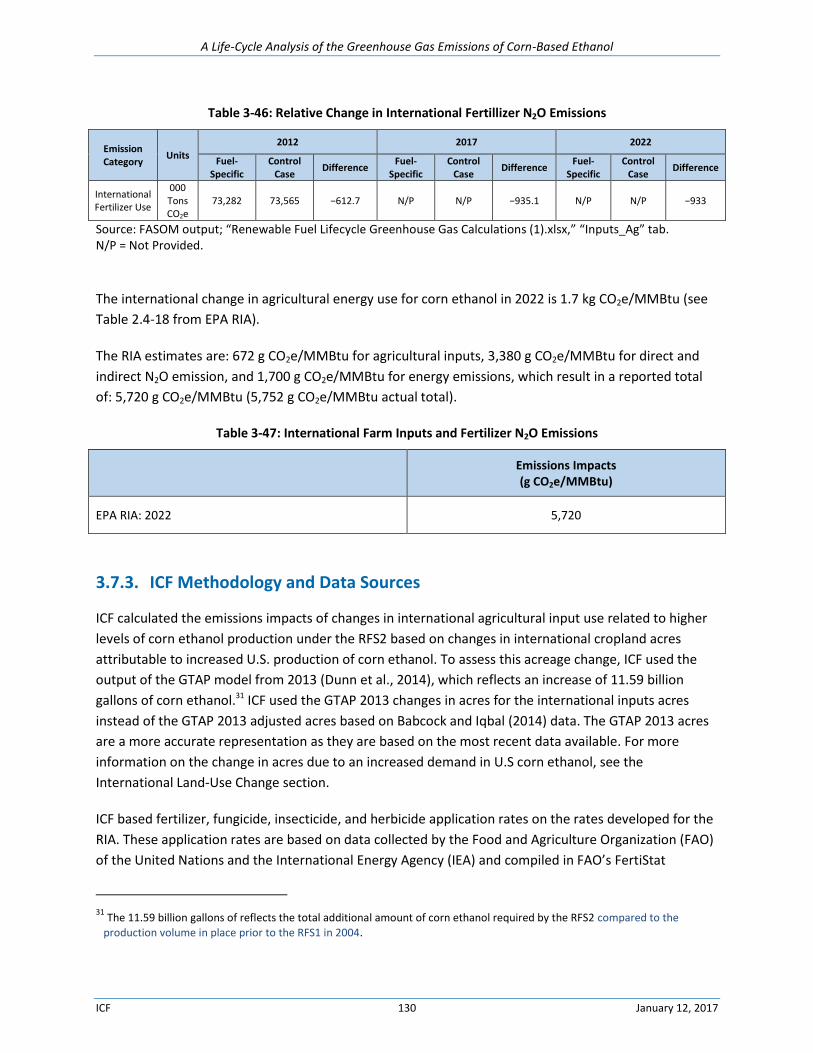
A Life-Cycle Analysis of the Greenhouse Gas Emissions of Corn-Based Ethanol
ICF 130 January 12, 2017
Table 3-46: Relative Change in International Fertillizer N2O Emissions
Emission Category
Units 2012 2017 2022
Fuel-Specific
Control Case
Difference Fuel-
Specific Control
Case Difference
Fuel-Specific
Control Case
Difference
International Fertilizer Use
000 Tons CO2e
73,282 73,565 −612.7 N/P N/P −935.1 N/P N/P −933
Source: FASOM output; “Renewable Fuel Lifecycle Greenhouse Gas Calculations (1).xlsx,” “Inputs_Ag” tab. N/P = Not Provided.
The international change in agricultural energy use for corn ethanol in 2022 is 1.7 kg CO2e/MMBtu (see
Table 2.4-18 from EPA RIA).
The RIA estimates are: 672 g CO2e/MMBtu for agricultural inputs, 3,380 g CO2e/MMBtu for direct and
indirect N2O emission, and 1,700 g CO2e/MMBtu for energy emissions, which result in a reported total
of: 5,720 g CO2e/MMBtu (5,752 g CO2e/MMBtu actual total).
Table 3-47: International Farm Inputs and Fertilizer N2O Emissions
Emissions Impacts (g CO2e/MMBtu)
EPA RIA: 2022 5,720
3.7.3. ICF Methodology and Data Sources
ICF calculated the emissions impacts of changes in international agricultural input use related to higher
levels of corn ethanol production under the RFS2 based on changes in international cropland acres
attributable to increased U.S. production of corn ethanol. To assess this acreage change, ICF used the
output of the GTAP model from 2013 (Dunn et al., 2014), which reflects an increase of 11.59 billion
gallons of corn ethanol.31 ICF used the GTAP 2013 changes in acres for the international inputs acres
instead of the GTAP 2013 adjusted acres based on Babcock and Iqbal (2014) data. The GTAP 2013 acres
are a more accurate representation as they are based on the most recent data available. For more
information on the change in acres due to an increased demand in U.S corn ethanol, see the
International Land-Use Change section.
ICF based fertilizer, fungicide, insecticide, and herbicide application rates on the rates developed for the
RIA. These application rates are based on data collected by the Food and Agriculture Organization (FAO)
of the United Nations and the International Energy Agency (IEA) and compiled in FAO’s FertiStat
31 The 11.59 billion gallons of reflects the total additional amount of corn ethanol required by the RFS2 compared to the
production volume in place prior to the RFS1 in 2004.
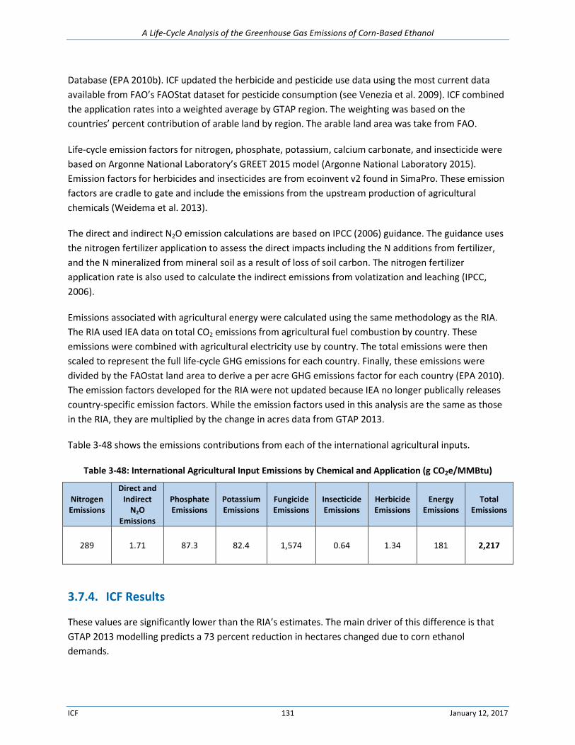
A Life-Cycle Analysis of the Greenhouse Gas Emissions of Corn-Based Ethanol
ICF 131 January 12, 2017
Database (EPA 2010b). ICF updated the herbicide and pesticide use data using the most current data
available from FAO’s FAOStat dataset for pesticide consumption (see Venezia et al. 2009). ICF combined
the application rates into a weighted average by GTAP region. The weighting was based on the
countries’ percent contribution of arable land by region. The arable land area was take from FAO.
Life-cycle emission factors for nitrogen, phosphate, potassium, calcium carbonate, and insecticide were
based on Argonne National Laboratory’s GREET 2015 model (Argonne National Laboratory 2015).
Emission factors for herbicides and insecticides are from ecoinvent v2 found in SimaPro. These emission
factors are cradle to gate and include the emissions from the upstream production of agricultural
chemicals (Weidema et al. 2013).
The direct and indirect N2O emission calculations are based on IPCC (2006) guidance. The guidance uses
the nitrogen fertilizer application to assess the direct impacts including the N additions from fertilizer,
and the N mineralized from mineral soil as a result of loss of soil carbon. The nitrogen fertilizer
application rate is also used to calculate the indirect emissions from volatization and leaching (IPCC,
2006).
Emissions associated with agricultural energy were calculated using the same methodology as the RIA.
The RIA used IEA data on total CO2 emissions from agricultural fuel combustion by country. These
emissions were combined with agricultural electricity use by country. The total emissions were then
scaled to represent the full life-cycle GHG emissions for each country. Finally, these emissions were
divided by the FAOstat land area to derive a per acre GHG emissions factor for each country (EPA 2010).
The emission factors developed for the RIA were not updated because IEA no longer publically releases
country-specific emission factors. While the emission factors used in this analysis are the same as those
in the RIA, they are multiplied by the change in acres data from GTAP 2013.
Table 3-48 shows the emissions contributions from each of the international agricultural inputs.
Table 3-48: International Agricultural Input Emissions by Chemical and Application (g CO2e/MMBtu)
Nitrogen Emissions
Direct and Indirect
N2O Emissions
Phosphate Emissions
Potassium Emissions
Fungicide Emissions
Insecticide Emissions
Herbicide Emissions
Energy Emissions
Total Emissions
289 1.71 87.3 82.4 1,574 0.64 1.34 181 2,217
3.7.4. ICF Results
These values are significantly lower than the RIA’s estimates. The main driver of this difference is that
GTAP 2013 modelling predicts a 73 percent reduction in hectares changed due to corn ethanol
demands.
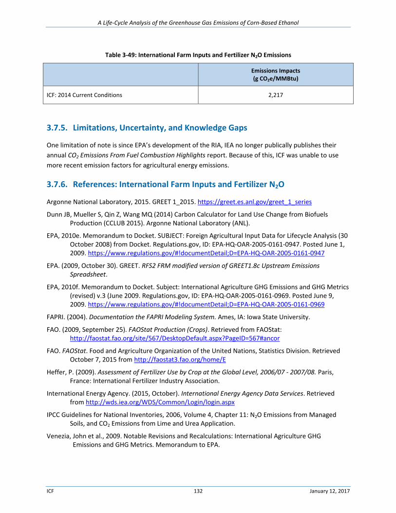
A Life-Cycle Analysis of the Greenhouse Gas Emissions of Corn-Based Ethanol
ICF 132 January 12, 2017
Table 3-49: International Farm Inputs and Fertilizer N2O Emissions
Emissions Impacts (g CO2e/MMBtu)
ICF: 2014 Current Conditions 2,217
3.7.5. Limitations, Uncertainty, and Knowledge Gaps
One limitation of note is since EPA’s development of the RIA, IEA no longer publically publishes their
annual CO2 Emissions From Fuel Combustion Highlights report. Because of this, ICF was unable to use
more recent emission factors for agricultural energy emissions.
3.7.6. References: International Farm Inputs and Fertilizer N2O
Argonne National Laboratory, 2015. GREET 1_2015. https://greet.es.anl.gov/greet_1_series
Dunn JB, Mueller S, Qin Z, Wang MQ (2014) Carbon Calculator for Land Use Change from Biofuels Production (CCLUB 2015). Argonne National Laboratory (ANL).
EPA, 2010e. Memorandum to Docket. SUBJECT: Foreign Agricultural Input Data for Lifecycle Analysis (30 October 2008) from Docket. Regulations.gov, ID: EPA-HQ-OAR-2005-0161-0947. Posted June 1, 2009. https://www.regulations.gov/#!documentDetail;D=EPA-HQ-OAR-2005-0161-0947
EPA. (2009, October 30). GREET. RFS2 FRM modified version of GREET1.8c Upstream Emissions Spreadsheet.
EPA, 2010f. Memorandum to Docket. Subject: International Agriculture GHG Emissions and GHG Metrics (revised) v.3 (June 2009. Regulations.gov, ID: EPA-HQ-OAR-2005-0161-0969. Posted June 9, 2009. https://www.regulations.gov/#!documentDetail;D=EPA-HQ-OAR-2005-0161-0969
FAPRI. (2004). Documentation the FAPRI Modeling System. Ames, IA: Iowa State University.
FAO. (2009, September 25). FAOStat Production (Crops). Retrieved from FAOStat: http://faostat.fao.org/site/567/DesktopDefault.aspx?PageID=567#ancor
FAO. FAOStat. Food and Argriculture Organization of the United Nations, Statistics Division. Retrieved October 7, 2015 from http://faostat3.fao.org/home/E
Heffer, P. (2009). Assessment of Fertilizer Use by Crop at the Global Level, 2006/07 - 2007/08. Paris, France: International Fertilizer Industry Association.
International Energy Agency. (2015, October). International Energy Agency Data Services. Retrieved from http://wds.iea.org/WDS/Common/Login/login.aspx
IPCC Guidelines for National Inventories, 2006, Volume 4, Chapter 11: N2O Emissions from Managed Soils, and CO2 Emissions from Lime and Urea Application.
Venezia, John et al., 2009. Notable Revisions and Recalculations: International Agriculture GHG Emissions and GHG Metrics. Memorandum to EPA.
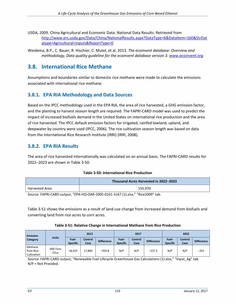
A Life-Cycle Analysis of the Greenhouse Gas Emissions of Corn-Based Ethanol
ICF 133 January 12, 2017
USDA, 2009. China Agricultural and Economic Data: National Data Results. Retrieved from http://www.ers.usda.gov/Data/China/NationalResults.aspx?DataType=6&DataItem=160&StrDatatype=Agricultural+inputs&ReportType=0
Weidema, B.P., C. Bauer, R. Hischier, C. Mutel, et al. 2013. The ecoinvent database: Overview and methodology, Data quality guideline for the ecoinvent database version 3. www.ecoinvent.org
3.8. International Rice Methane
Assumptions and boundaries similar to domestic rice methane were made to calculate the emissions
associated with international rice methane.
3.8.1. EPA RIA Methodology and Data Sources
Based on the IPCC methodology used in the EPA RIA, the area of rice harvested, a GHG emission factor,
and the planting to harvest season length are required. The FAPRI-CARD model was used to predict the
impact of increased biofuels demand in the United States on international rice production and the area
of rice harvested. The IPCC default emission factors for irrigated, rainfed lowland, upland, and
deepwater by country were used (IPCC, 2006). The rice cultivation season length was based on data
from the International Rice Research Institute (IRRI) (IRRI, 2008).
3.8.2. EPA RIA Results
The area of rice harvested internationally was calculated on an annual basis. The FAPRI-CARD results for
2022–2023 are shown in Table 3-50.
Table 3-50: International Rice Production
Thousand Acres Harvested in 2022–2023
Harvested Area 155,970
Source: FAPRI-CARD output; “EPA-HQ-OAR-2005-0161-3167 (1).xlsx,” “Rice2009” tab.
Table 3-51 shows the emissions as a result of land-use change from increased demand from biofuels and
converting land from rice acres to corn acres.
Table 3-51: Relative Change in International Methane from Rice Production
Emission Category
Units 2012 2017 2022
Fuel-Specific
Control Case
Difference Fuel-
Specific Control
Case Difference
Fuel-Specific
Control Case
Difference
Methane from Rice Cultivation
000 Tons CO2e
18,410 17,800 −359.8 N/P N/P −227.5 N/P N/P −352
Source: FAPRI-CARD output; “Renewable Fuel Lifecycle Greenhouse Gas Calculations (1).xlsx,” “Input_Ag” tab. N/P = Not Provided.
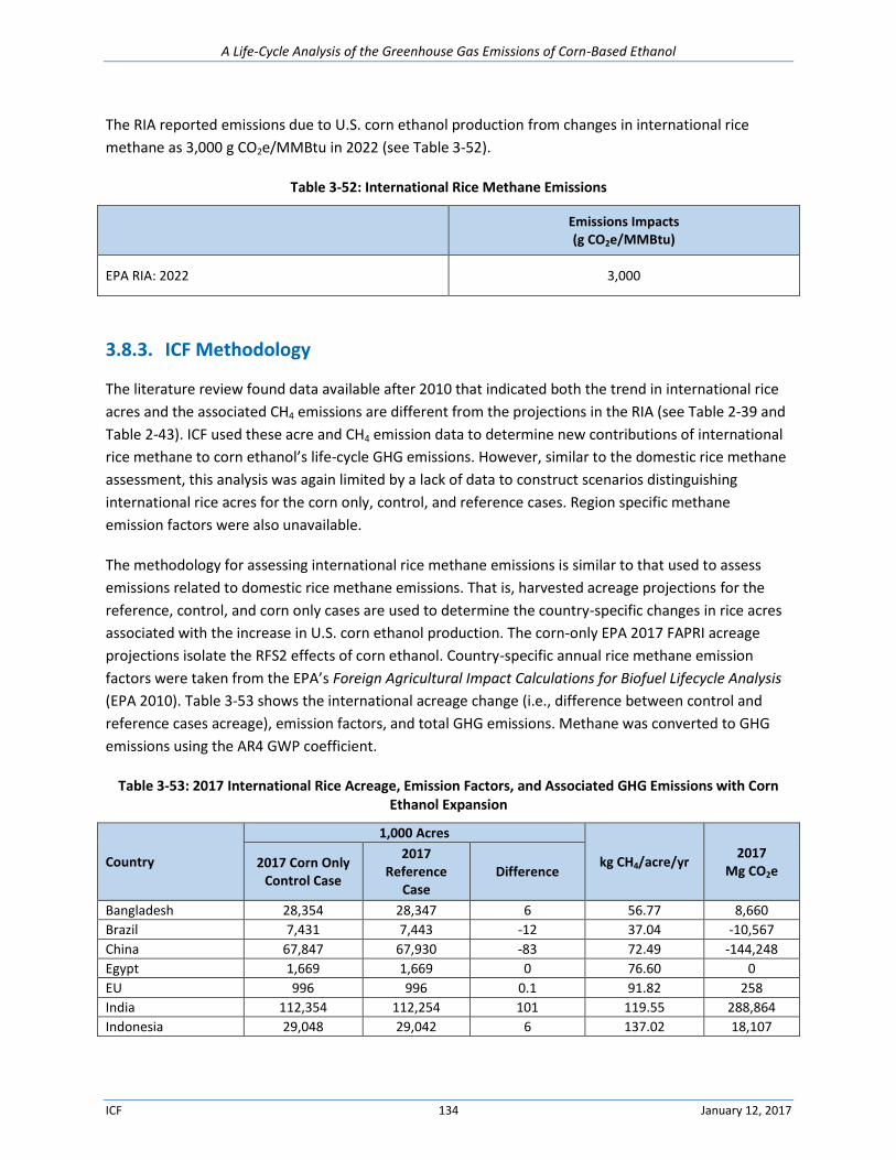
A Life-Cycle Analysis of the Greenhouse Gas Emissions of Corn-Based Ethanol
ICF 134 January 12, 2017
The RIA reported emissions due to U.S. corn ethanol production from changes in international rice
methane as 3,000 g CO2e/MMBtu in 2022 (see Table 3-52).
Table 3-52: International Rice Methane Emissions
Emissions Impacts (g CO2e/MMBtu)
EPA RIA: 2022 3,000
3.8.3. ICF Methodology
The literature review found data available after 2010 that indicated both the trend in international rice
acres and the associated CH4 emissions are different from the projections in the RIA (see Table 2-39 and
Table 2-43). ICF used these acre and CH4 emission data to determine new contributions of international
rice methane to corn ethanol’s life-cycle GHG emissions. However, similar to the domestic rice methane
assessment, this analysis was again limited by a lack of data to construct scenarios distinguishing
international rice acres for the corn only, control, and reference cases. Region specific methane
emission factors were also unavailable.
The methodology for assessing international rice methane emissions is similar to that used to assess
emissions related to domestic rice methane emissions. That is, harvested acreage projections for the
reference, control, and corn only cases are used to determine the country-specific changes in rice acres
associated with the increase in U.S. corn ethanol production. The corn-only EPA 2017 FAPRI acreage
projections isolate the RFS2 effects of corn ethanol. Country-specific annual rice methane emission
factors were taken from the EPA’s Foreign Agricultural Impact Calculations for Biofuel Lifecycle Analysis
(EPA 2010). Table 3-53 shows the international acreage change (i.e., difference between control and
reference cases acreage), emission factors, and total GHG emissions. Methane was converted to GHG
emissions using the AR4 GWP coefficient.
Table 3-53: 2017 International Rice Acreage, Emission Factors, and Associated GHG Emissions with Corn Ethanol Expansion
Country
1,000 Acres
kg CH4/acre/yr 2017
Mg CO2e 2017 Corn Only
Control Case
2017 Reference
Case Difference
Bangladesh 28,354 28,347 6 56.77 8,660
Brazil 7,431 7,443 -12 37.04 -10,567
China 67,847 67,930 -83 72.49 -144,248
Egypt 1,669 1,669 0 76.60 0
EU 996 996 0.1 91.82 258
India 112,354 112,254 101 119.55 288,864
Indonesia 29,048 29,042 6 137.02 18,107
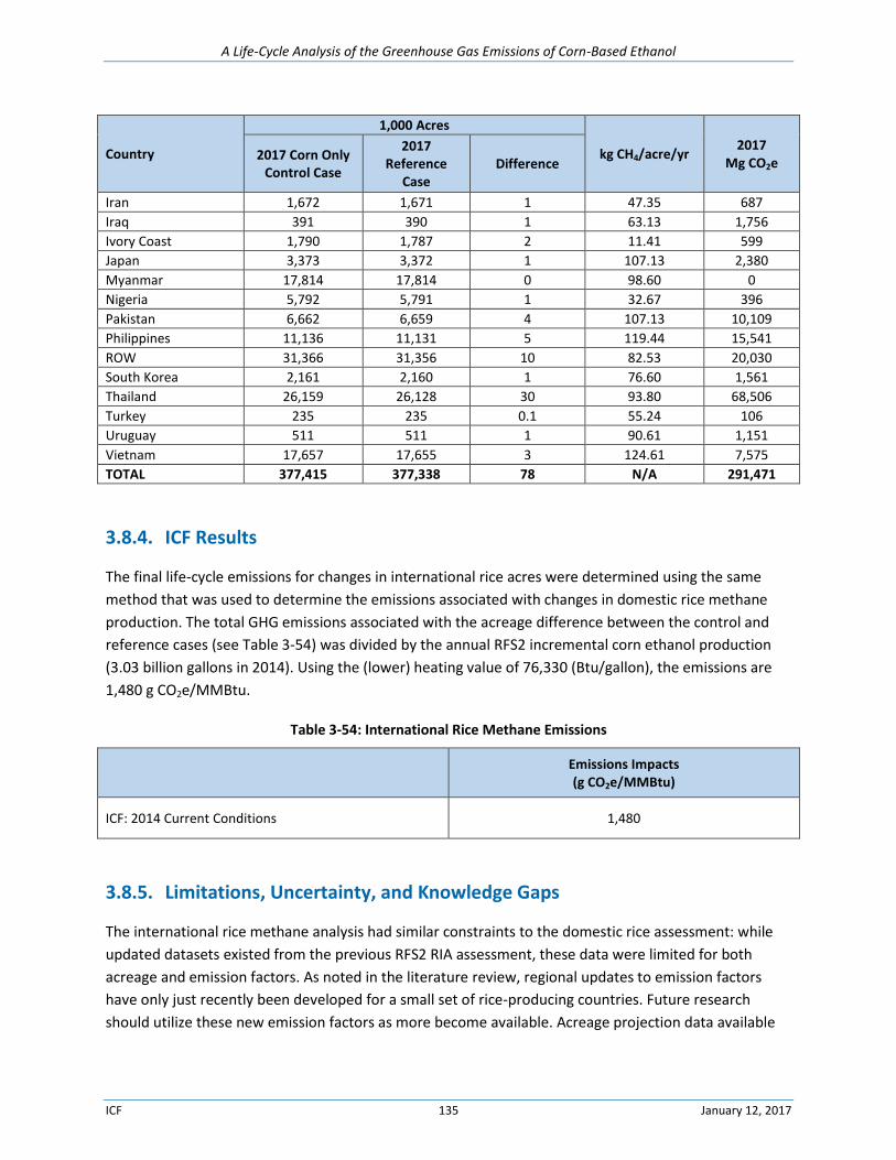
A Life-Cycle Analysis of the Greenhouse Gas Emissions of Corn-Based Ethanol
ICF 135 January 12, 2017
Country
1,000 Acres
kg CH4/acre/yr 2017
Mg CO2e 2017 Corn Only
Control Case
2017 Reference
Case Difference
Iran 1,672 1,671 1 47.35 687
Iraq 391 390 1 63.13 1,756
Ivory Coast 1,790 1,787 2 11.41 599
Japan 3,373 3,372 1 107.13 2,380
Myanmar 17,814 17,814 0 98.60 0
Nigeria 5,792 5,791 1 32.67 396
Pakistan 6,662 6,659 4 107.13 10,109
Philippines 11,136 11,131 5 119.44 15,541
ROW 31,366 31,356 10 82.53 20,030
South Korea 2,161 2,160 1 76.60 1,561
Thailand 26,159 26,128 30 93.80 68,506
Turkey 235 235 0.1 55.24 106
Uruguay 511 511 1 90.61 1,151
Vietnam 17,657 17,655 3 124.61 7,575
TOTAL 377,415 377,338 78 N/A 291,471
3.8.4. ICF Results
The final life-cycle emissions for changes in international rice acres were determined using the same
method that was used to determine the emissions associated with changes in domestic rice methane
production. The total GHG emissions associated with the acreage difference between the control and
reference cases (see Table 3-54) was divided by the annual RFS2 incremental corn ethanol production
(3.03 billion gallons in 2014). Using the (lower) heating value of 76,330 (Btu/gallon), the emissions are
1,480 g CO2e/MMBtu.
Table 3-54: International Rice Methane Emissions
Emissions Impacts (g CO2e/MMBtu)
ICF: 2014 Current Conditions 1,480
3.8.5. Limitations, Uncertainty, and Knowledge Gaps
The international rice methane analysis had similar constraints to the domestic rice assessment: while
updated datasets existed from the previous RFS2 RIA assessment, these data were limited for both
acreage and emission factors. As noted in the literature review, regional updates to emission factors
have only just recently been developed for a small set of rice-producing countries. Future research
should utilize these new emission factors as more become available. Acreage projection data available
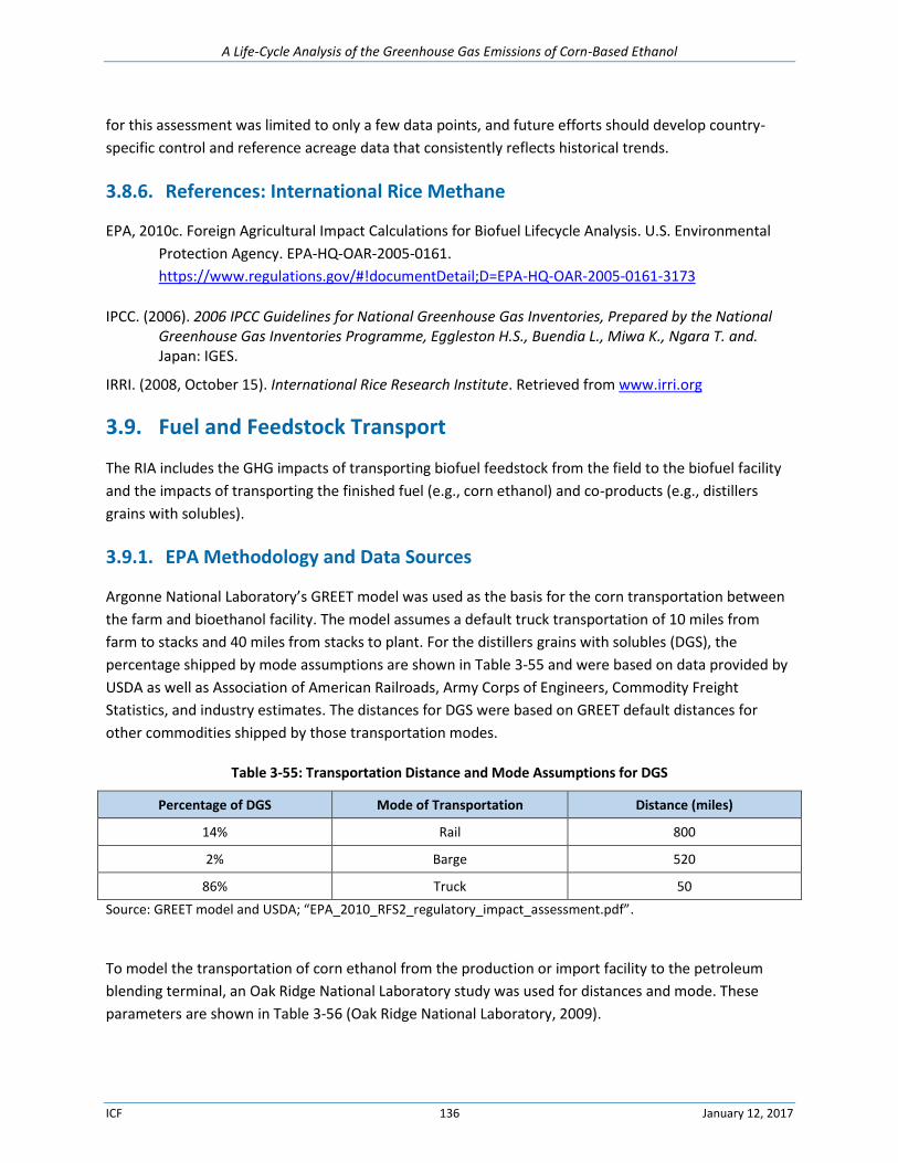
A Life-Cycle Analysis of the Greenhouse Gas Emissions of Corn-Based Ethanol
ICF 136 January 12, 2017
for this assessment was limited to only a few data points, and future efforts should develop country-
specific control and reference acreage data that consistently reflects historical trends.
3.8.6. References: International Rice Methane
EPA, 2010c. Foreign Agricultural Impact Calculations for Biofuel Lifecycle Analysis. U.S. Environmental
Protection Agency. EPA‐HQ‐OAR‐2005‐0161.
https://www.regulations.gov/#!documentDetail;D=EPA-HQ-OAR-2005-0161-3173
IPCC. (2006). 2006 IPCC Guidelines for National Greenhouse Gas Inventories, Prepared by the National Greenhouse Gas Inventories Programme, Eggleston H.S., Buendia L., Miwa K., Ngara T. and. Japan: IGES.
IRRI. (2008, October 15). International Rice Research Institute. Retrieved from www.irri.org
3.9. Fuel and Feedstock Transport
The RIA includes the GHG impacts of transporting biofuel feedstock from the field to the biofuel facility
and the impacts of transporting the finished fuel (e.g., corn ethanol) and co-products (e.g., distillers
grains with solubles).
3.9.1. EPA Methodology and Data Sources
Argonne National Laboratory’s GREET model was used as the basis for the corn transportation between
the farm and bioethanol facility. The model assumes a default truck transportation of 10 miles from
farm to stacks and 40 miles from stacks to plant. For the distillers grains with solubles (DGS), the
percentage shipped by mode assumptions are shown in Table 3-55 and were based on data provided by
USDA as well as Association of American Railroads, Army Corps of Engineers, Commodity Freight
Statistics, and industry estimates. The distances for DGS were based on GREET default distances for
other commodities shipped by those transportation modes.
Table 3-55: Transportation Distance and Mode Assumptions for DGS
Percentage of DGS Mode of Transportation Distance (miles)
14% Rail 800
2% Barge 520
86% Truck 50
Source: GREET model and USDA; “EPA_2010_RFS2_regulatory_impact_assessment.pdf”.
To model the transportation of corn ethanol from the production or import facility to the petroleum
blending terminal, an Oak Ridge National Laboratory study was used for distances and mode. These
parameters are shown in Table 3-56 (Oak Ridge National Laboratory, 2009).
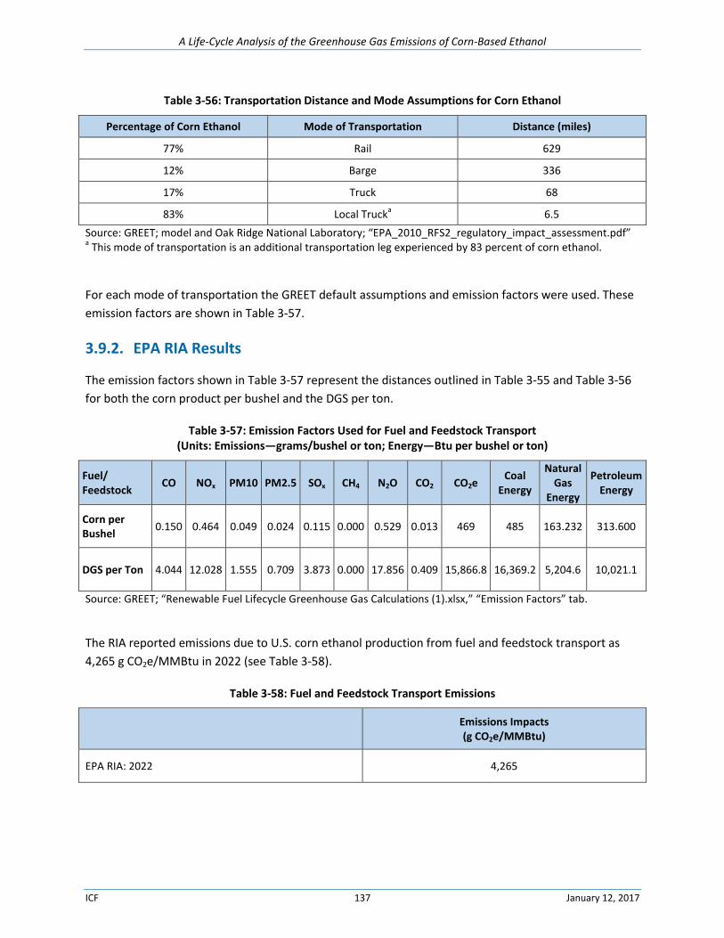
A Life-Cycle Analysis of the Greenhouse Gas Emissions of Corn-Based Ethanol
ICF 137 January 12, 2017
Table 3-56: Transportation Distance and Mode Assumptions for Corn Ethanol
Percentage of Corn Ethanol Mode of Transportation Distance (miles)
77% Rail 629
12% Barge 336
17% Truck 68
83% Local Trucka 6.5
Source: GREET; model and Oak Ridge National Laboratory; “EPA_2010_RFS2_regulatory_impact_assessment.pdf” a This mode of transportation is an additional transportation leg experienced by 83 percent of corn ethanol.
For each mode of transportation the GREET default assumptions and emission factors were used. These
emission factors are shown in Table 3-57.
3.9.2. EPA RIA Results
The emission factors shown in Table 3-57 represent the distances outlined in Table 3-55 and Table 3-56
for both the corn product per bushel and the DGS per ton.
Table 3-57: Emission Factors Used for Fuel and Feedstock Transport (Units: Emissions—grams/bushel or ton; Energy—Btu per bushel or ton)
Fuel/ Feedstock
CO NOx PM10 PM2.5 SOx CH4 N2O CO2 CO2e Coal
Energy
Natural Gas
Energy
Petroleum Energy
Corn per Bushel
0.150 0.464 0.049 0.024 0.115 0.000 0.529 0.013 469 485 163.232 313.600
DGS per Ton 4.044 12.028 1.555 0.709 3.873 0.000 17.856 0.409 15,866.8 16,369.2 5,204.6 10,021.1
Source: GREET; “Renewable Fuel Lifecycle Greenhouse Gas Calculations (1).xlsx,” “Emission Factors” tab.
The RIA reported emissions due to U.S. corn ethanol production from fuel and feedstock transport as
4,265 g CO2e/MMBtu in 2022 (see Table 3-58).
Table 3-58: Fuel and Feedstock Transport Emissions
Emissions Impacts (g CO2e/MMBtu)
EPA RIA: 2022 4,265
A Life-Cycle Analysis of the Greenhouse Gas Emissions of Corn-Based Ethanol
ICF 138 January 12, 2017
3.9.3. ICF Methodology
Fuel and feedstock transportation represents a minimal portion of total corn ethanol life-cycle GHG
emissions, contributing less than 5 percent (EPA, 2010a). However, transportation systems are dynamic
and since 2010 have continually evolved to become more fuel and GHG efficient. Key developments
that may have affected the GHG LCA profile of corn ethanol include:
Improved transportation technologies, such as improved fuel economies for medium and heavy
duty (MDHD) diesel trucks (Cai et al., 2015).
Infrastructure retrofits, such as utilizing existing liquid fuel pipelines for ethanol transport (Strogen
et al., 2013).
Decreasing GHG intensity of the average fuel mix used in transportation (Cai et al., 2015).
Given these potential sources of GHG reductions, our assessment applied the latest data and emission
factors using a similar methodology to the EPA’s report.
Figure 3-5 illustrates the stages involved in fuel and feedstock transportation based on the most recent
GREET model.
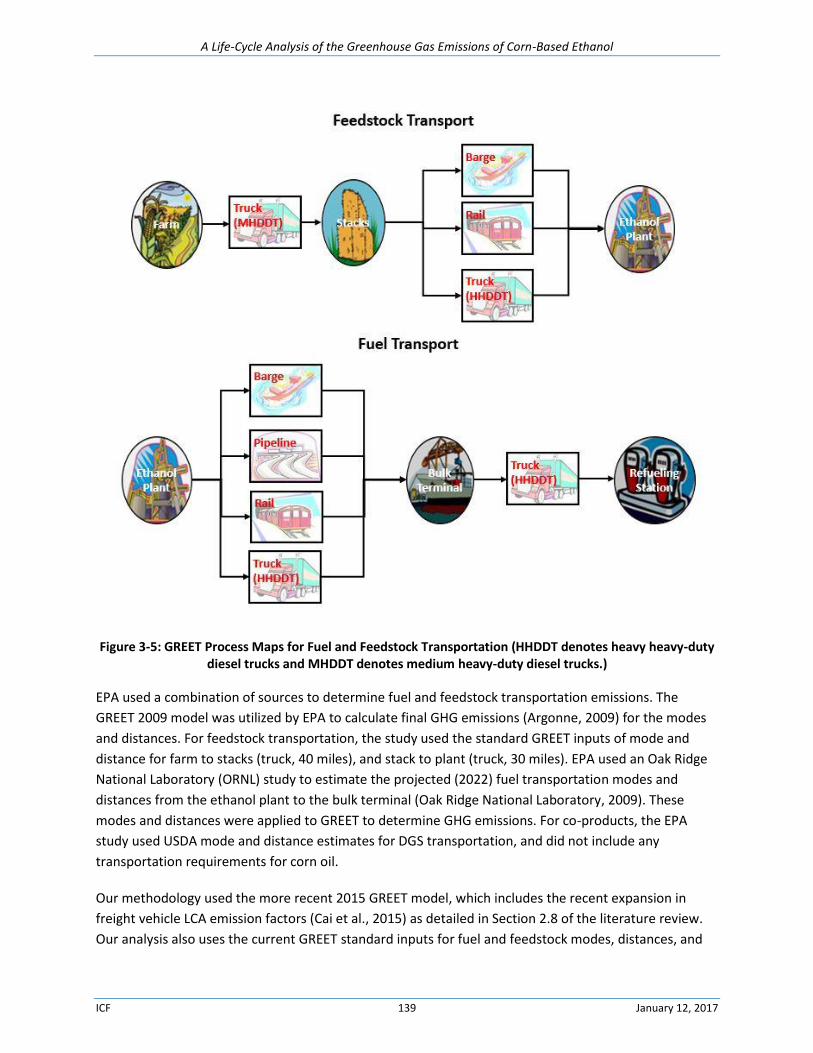
A Life-Cycle Analysis of the Greenhouse Gas Emissions of Corn-Based Ethanol
ICF 139 January 12, 2017
Figure 3-5: GREET Process Maps for Fuel and Feedstock Transportation (HHDDT denotes heavy heavy-duty diesel trucks and MHDDT denotes medium heavy-duty diesel trucks.)
EPA used a combination of sources to determine fuel and feedstock transportation emissions. The
GREET 2009 model was utilized by EPA to calculate final GHG emissions (Argonne, 2009) for the modes
and distances. For feedstock transportation, the study used the standard GREET inputs of mode and
distance for farm to stacks (truck, 40 miles), and stack to plant (truck, 30 miles). EPA used an Oak Ridge
National Laboratory (ORNL) study to estimate the projected (2022) fuel transportation modes and
distances from the ethanol plant to the bulk terminal (Oak Ridge National Laboratory, 2009). These
modes and distances were applied to GREET to determine GHG emissions. For co-products, the EPA
study used USDA mode and distance estimates for DGS transportation, and did not include any
transportation requirements for corn oil.
Our methodology used the more recent 2015 GREET model, which includes the recent expansion in
freight vehicle LCA emission factors (Cai et al., 2015) as detailed in Section 2.8 of the literature review.
Our analysis also uses the current GREET standard inputs for fuel and feedstock modes, distances, and
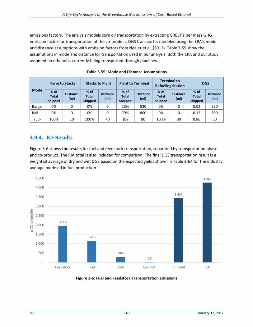
A Life-Cycle Analysis of the Greenhouse Gas Emissions of Corn-Based Ethanol
ICF 140 January 12, 2017
emissions factors. The analysis models corn oil transportation by extracting GREET’s per mass GHG
emission factor for transportation of the co-product. DGS transport is modeled using the EPA’s mode
and distance assumptions with emission factors from Nealer et al. (2012). Table 3-59 show the
assumptions in mode and distance for transportation used in our analysis. Both the EPA and our study
assumed no ethanol is currently being transported through pipelines.
Table 3-59: Mode and Distance Assumptions
Mode
Farm to Stacks Stacks to Plant Plant to Terminal Terminal to
Refueling Station DGS
% of Total
Shipped
Distance (mi)
% of Total
Shipped
Distance (mi)
% of Total
Shipped
Distance (mi)
% of Total
Shipped
Distance (mi)
% of Total
Shipped
Distance (mi)
Barge 0% 0 0% 0 13% 520 0% 0 0.02 520
Rail 0% 0 0% 0 79% 800 0% 0 0.12 800
Truck 100% 10 100% 40 8% 80 100% 30 0.86 50
3.9.4. ICF Results
Figure 3-6 shows the results for fuel and feedstock transportation, separated by transportation phase
and co-product. The RIA total is also included for comparison. The final DGS transportation result is a
weighted average of dry and wet DGS based on the expected yields shown in Table 3-64 for the industry
average modeled in fuel production.
Figure 3-6: Fuel and Feedstock Transportation Emissions
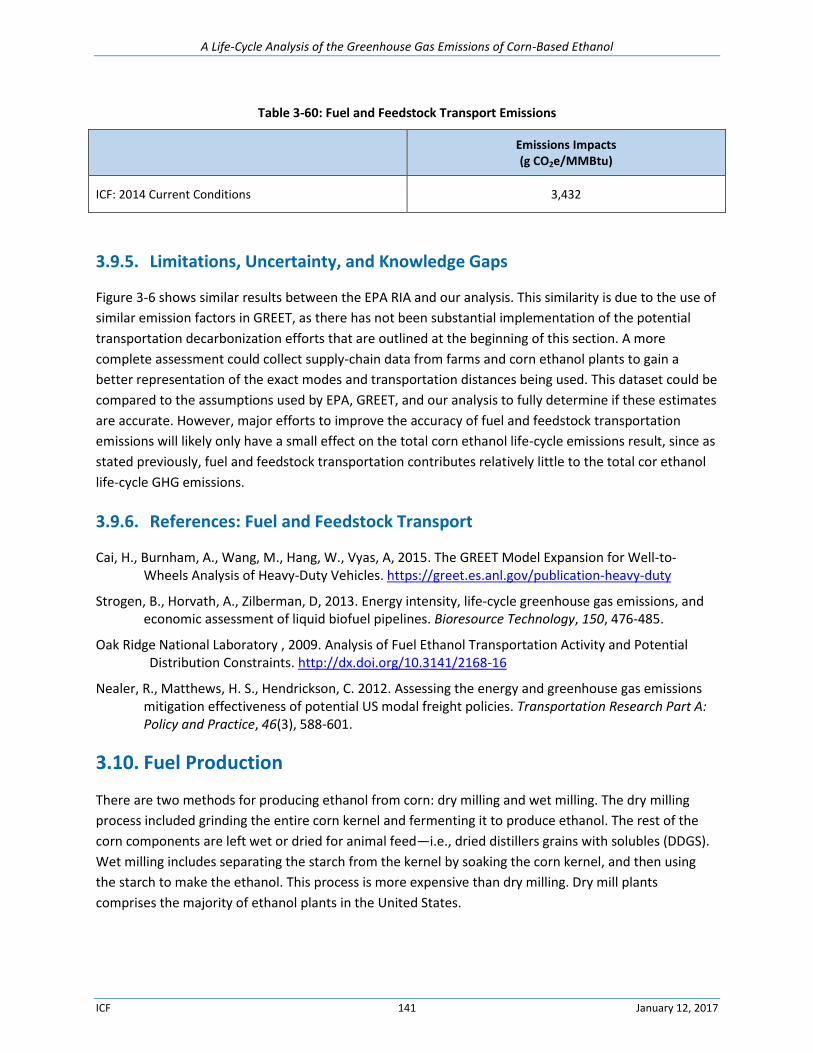
A Life-Cycle Analysis of the Greenhouse Gas Emissions of Corn-Based Ethanol
ICF 141 January 12, 2017
Table 3-60: Fuel and Feedstock Transport Emissions
Emissions Impacts (g CO2e/MMBtu)
ICF: 2014 Current Conditions 3,432
3.9.5. Limitations, Uncertainty, and Knowledge Gaps
Figure 3-6 shows similar results between the EPA RIA and our analysis. This similarity is due to the use of
similar emission factors in GREET, as there has not been substantial implementation of the potential
transportation decarbonization efforts that are outlined at the beginning of this section. A more
complete assessment could collect supply-chain data from farms and corn ethanol plants to gain a
better representation of the exact modes and transportation distances being used. This dataset could be
compared to the assumptions used by EPA, GREET, and our analysis to fully determine if these estimates
are accurate. However, major efforts to improve the accuracy of fuel and feedstock transportation
emissions will likely only have a small effect on the total corn ethanol life-cycle emissions result, since as
stated previously, fuel and feedstock transportation contributes relatively little to the total cor ethanol
life-cycle GHG emissions.
3.9.6. References: Fuel and Feedstock Transport
Cai, H., Burnham, A., Wang, M., Hang, W., Vyas, A, 2015. The GREET Model Expansion for Well-to-Wheels Analysis of Heavy-Duty Vehicles. https://greet.es.anl.gov/publication-heavy-duty
Strogen, B., Horvath, A., Zilberman, D, 2013. Energy intensity, life-cycle greenhouse gas emissions, and economic assessment of liquid biofuel pipelines. Bioresource Technology, 150, 476-485.
Oak Ridge National Laboratory , 2009. Analysis of Fuel Ethanol Transportation Activity and Potential Distribution Constraints. http://dx.doi.org/10.3141/2168-16
Nealer, R., Matthews, H. S., Hendrickson, C. 2012. Assessing the energy and greenhouse gas emissions mitigation effectiveness of potential US modal freight policies. Transportation Research Part A: Policy and Practice, 46(3), 588-601.
3.10. Fuel Production
There are two methods for producing ethanol from corn: dry milling and wet milling. The dry milling
process included grinding the entire corn kernel and fermenting it to produce ethanol. The rest of the
corn components are left wet or dried for animal feed—i.e., dried distillers grains with solubles (DDGS).
Wet milling includes separating the starch from the kernel by soaking the corn kernel, and then using
the starch to make the ethanol. This process is more expensive than dry milling. Dry mill plants
comprises the majority of ethanol plants in the United States.
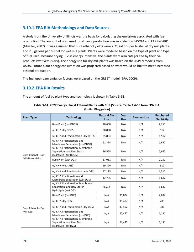
A Life-Cycle Analysis of the Greenhouse Gas Emissions of Corn-Based Ethanol
ICF 142 January 12, 2017
3.10.1. EPA RIA Methodology and Data Sources
A study from the University of Illinois was the basis for calculating the emissions associated with fuel
production. The amount of corn used for ethanol production was modeled by FASOM and FAPRI-CARD
(Mueller, 2007). It was assumed that pure ethanol yields were 2.71 gallons per bushel at dry mill plants
and 2.5 gallons per bushel for wet mill plants. Plants were modeled based on the type of plant and type
of fuel used. Because drying DGS is energy intensive, the plants were also categorized by their co-
products (wet versus dry). The energy use for dry mill plants was based on the ASPEN models from
USDA. Future plant energy consumption was projected based on what would be built to meet increased
ethanol production.
The fuel upstream emission factors were based on the GREET model (EPA, 2009).
3.10.2. EPA RIA Results
The amount of fuel by plant type and technology is shown in Table 3-61.
Table 3-61: 2022 Energy Use at Ethanol Plants with CHP (Source: Table 2.4-55 from EPA RIA) (Units: Btu/gallon)
Plant Type Technology Natural Gas
Use Coal Use
Biomass Use Purchased Electricity
Corn Ethanol—Dry Mill-Natural Gas
Base Plant (dry DDGS) 28,660 N/A N/A 2,251
w/ CHP (dry DDGS) 30,898 N/A N/A 512
w/ CHP and Fractionation (dry DDGS) 25,854 N/A N/A 1,512
w/ CHP, Fractionation, and Membrane Separation (dry DDGS)
21,354 N/A N/A 1,682
w/ CHP, Fractionation, Membrane Separation, and Raw Starch Hydrolysis (dry DDGS)
16,568 N/A N/A 1,682
Base Plant (wet DGS) 17,081 N/A N/A 2,251
w/ CHP (wet DGS) 19,320 N/A N/A 512
w/ CHP and Fractionation (wet DGS) 17,285 N/A N/A 1,512
w/ CHP, Fractionation and Membrane Separation (wet DGS)
12,785 N/A N/A 1,682
w/ CHP, Fractionation, Membrane Separation, and Raw Starch Hydrolysis (wet DGS)
9,932 N/A N/A 1,682
Corn Ethanol—Dry Mill-Coal
Base Plant (dry DGS) N/A 35,824 N/A 2,694
w/ CHP (dry DGS) N/A 39,407 N/A 205
w/ CHP and Fractionation (dry DGS) N/A 33,102 N/A 986
w/ CHP, Fractionation, and Membrane Separation (dry DGS)
N/A 27,477 N/A 1,191
w/ CHP, Fractionation, Membrane Separation, and Raw Starch Hydrolysis (dry DGS)
N/A 21,495 N/A 1,191
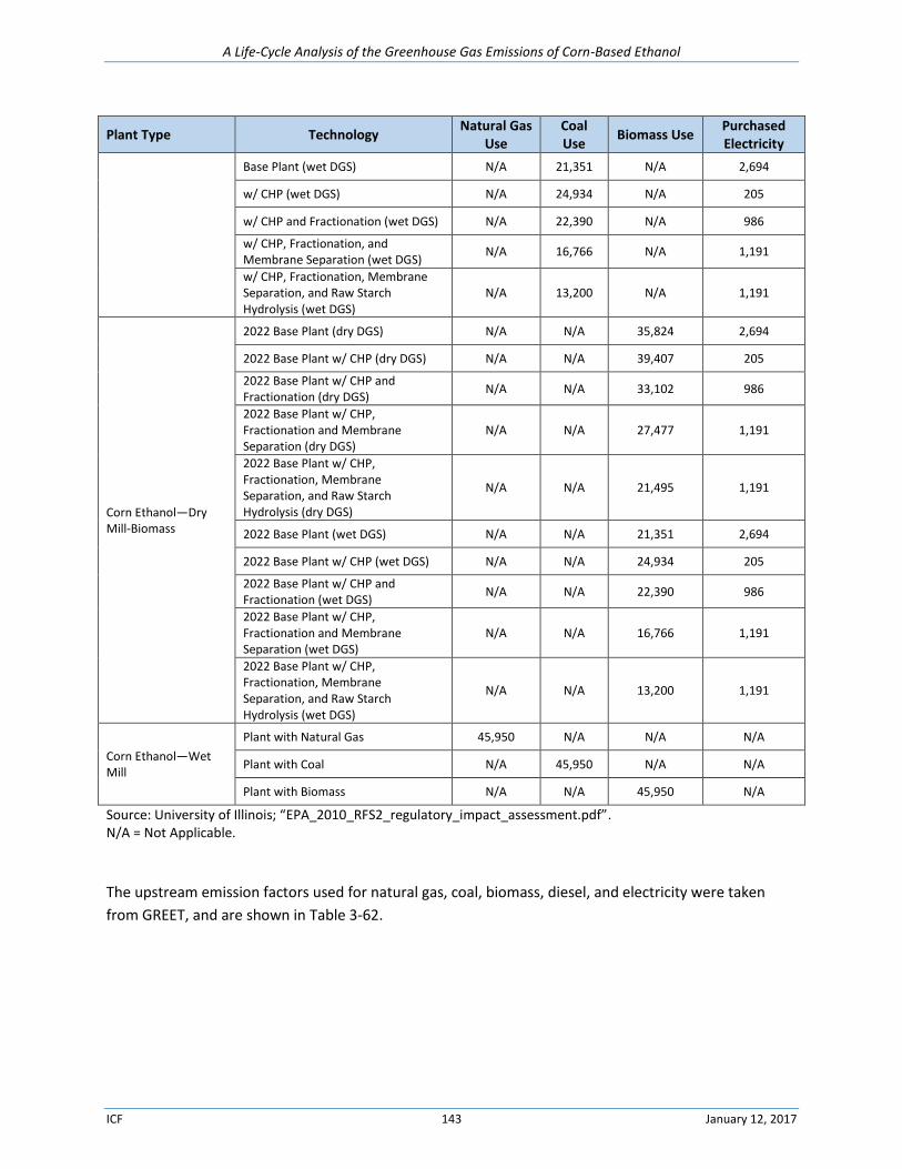
A Life-Cycle Analysis of the Greenhouse Gas Emissions of Corn-Based Ethanol
ICF 143 January 12, 2017
Plant Type Technology Natural Gas
Use Coal Use
Biomass Use Purchased Electricity
Base Plant (wet DGS) N/A 21,351 N/A 2,694
w/ CHP (wet DGS) N/A 24,934 N/A 205
w/ CHP and Fractionation (wet DGS) N/A 22,390 N/A 986
w/ CHP, Fractionation, and Membrane Separation (wet DGS)
N/A 16,766 N/A 1,191
w/ CHP, Fractionation, Membrane Separation, and Raw Starch Hydrolysis (wet DGS)
N/A 13,200 N/A 1,191
Corn Ethanol—Dry Mill-Biomass
2022 Base Plant (dry DGS) N/A N/A 35,824 2,694
2022 Base Plant w/ CHP (dry DGS) N/A N/A 39,407 205
2022 Base Plant w/ CHP and Fractionation (dry DGS)
N/A N/A 33,102 986
2022 Base Plant w/ CHP, Fractionation and Membrane Separation (dry DGS)
N/A N/A 27,477 1,191
2022 Base Plant w/ CHP, Fractionation, Membrane Separation, and Raw Starch Hydrolysis (dry DGS)
N/A N/A 21,495 1,191
2022 Base Plant (wet DGS) N/A N/A 21,351 2,694
2022 Base Plant w/ CHP (wet DGS) N/A N/A 24,934 205
2022 Base Plant w/ CHP and Fractionation (wet DGS)
N/A N/A 22,390 986
2022 Base Plant w/ CHP, Fractionation and Membrane Separation (wet DGS)
N/A N/A 16,766 1,191
2022 Base Plant w/ CHP, Fractionation, Membrane Separation, and Raw Starch Hydrolysis (wet DGS)
N/A N/A 13,200 1,191
Corn Ethanol—Wet Mill
Plant with Natural Gas 45,950 N/A N/A N/A
Plant with Coal N/A 45,950 N/A N/A
Plant with Biomass N/A N/A 45,950 N/A
Source: University of Illinois; “EPA_2010_RFS2_regulatory_impact_assessment.pdf”. N/A = Not Applicable.
The upstream emission factors used for natural gas, coal, biomass, diesel, and electricity were taken
from GREET, and are shown in Table 3-62.
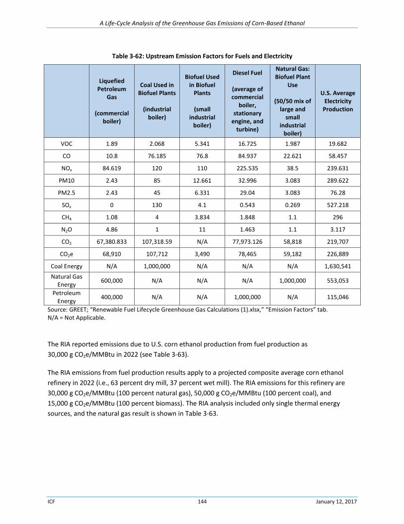
A Life-Cycle Analysis of the Greenhouse Gas Emissions of Corn-Based Ethanol
ICF 144 January 12, 2017
Table 3-62: Upstream Emission Factors for Fuels and Electricity
Liquefied Petroleum
Gas
(commercial boiler)
Coal Used in Biofuel Plants
(industrial
boiler)
Biofuel Used in Biofuel
Plants
(small industrial
boiler)
Diesel Fuel
(average of commercial
boiler, stationary
engine, and turbine)
Natural Gas: Biofuel Plant
Use
(50/50 mix of large and
small industrial
boiler)
U.S. Average Electricity
Production
VOC 1.89 2.068 5.341 16.725 1.987 19.682
CO 10.8 76.185 76.8 84.937 22.621 58.457
NOx 84.619 120 110 225.535 38.5 239.631
PM10 2.43 85 12.661 32.996 3.083 289.622
PM2.5 2.43 45 6.331 29.04 3.083 76.28
SOx 0 130 4.1 0.543 0.269 527.218
CH4 1.08 4 3.834 1.848 1.1 296
N2O 4.86 1 11 1.463 1.1 3.117
CO2 67,380.833 107,318.59 N/A 77,973.126 58,818 219,707
CO2e 68,910 107,712 3,490 78,465 59,182 226,889
Coal Energy N/A 1,000,000 N/A N/A N/A 1,630,541
Natural Gas Energy
600,000 N/A N/A N/A 1,000,000 553,053
Petroleum Energy
400,000 N/A N/A 1,000,000 N/A 115,046
Source: GREET; “Renewable Fuel Lifecycle Greenhouse Gas Calculations (1).xlsx,” “Emission Factors” tab. N/A = Not Applicable.
The RIA reported emissions due to U.S. corn ethanol production from fuel production as
30,000 g CO2e/MMBtu in 2022 (see Table 3-63).
The RIA emissions from fuel production results apply to a projected composite average corn ethanol
refinery in 2022 (i.e., 63 percent dry mill, 37 percent wet mill). The RIA emissions for this refinery are
30,000 g CO2e/MMBtu (100 percent natural gas), 50,000 g CO2e/MMBtu (100 percent coal), and
15,000 g CO2e/MMBtu (100 percent biomass). The RIA analysis included only single thermal energy
sources, and the natural gas result is shown in Table 3-63.
A Life-Cycle Analysis of the Greenhouse Gas Emissions of Corn-Based Ethanol
ICF 145 January 12, 2017
Table 3-63: Fuel Production Emissions
Emissions Impacts (g CO2e/MMBtu)
EPA RIA: 2022 30,000
3.10.3. ICF Methodology
Corn-ethanol production has experienced considerable growth since 2010. From 2009–2014, U.S. fuel
ethanol production increased by 40 percent, reaching over 14 billion gallons annually (EIA 2013, EIA
2015). There are currently 14 newly proposed and under-construction production plants, which will add
over 850 million gallons per year to U.S. capacity (Ethanol Producer Magazine 2016).
With this growth have come improved process efficiencies and new co-products. These process
upgrades have become drivers for a decreasing GHG-intensity of corn ethanol production. Production
yields, measured in gallons of ethanol per bushel of corn, increased by 5 percent between 2006 and
2014. New enzymes and yeast strains have increased process efficiencies in starch conversion and
fermentation (EIA 2015). Along with distillers grains and solubles (DGS), corn oil is now recovered as a
co-product, and 80 percent of dry grind mills are now capable of corn oil recovery (Argonne 2014). New
state and federal programs, such as EPA’s Efficient Producer Program and California’s Low Carbon Fuel
Standard, create incentives for innovative efforts that continue to lower corn ethanol production GHG
emissions.
The RIA used process-level data for energy use at corn ethanol production facilities. The data accounted
for both dry and wet mill processes, where EPA modeled variations of primary energy (i.e., coal, natural
gas, biomass) and electricity demands. The wet mill model did not include any electricity use. For the dry
mill model, five process variations were modeled for both dry and wet DGS outputs (i.e., 10 total):
Base plant
Combined heat and power (CHP)
CHP with corn oil fractionation
CHP with fractionation and membrane separation
CHP with fractionation, membrane separation, and raw starch hydrolysis
The study restricted wet milling variations to only three primary energy use variations (100 percent
natural gas, 100 percent coal, 100 percent biomass). The final average plant results were based on a
combination of dry milling with fractionation (63 percent) and wet milling (37 percent), where both
processes used natural gas as the primary energy source.
Our analysis uses more recent corn ethanol production data and emission factors available to estimate
the current GHG intensity of production processes. The modeling utilizes the more recent GREET corn
ethanol pathway updates (Argonne 2014), which use process-level data from Mueller and Kwik (2012).
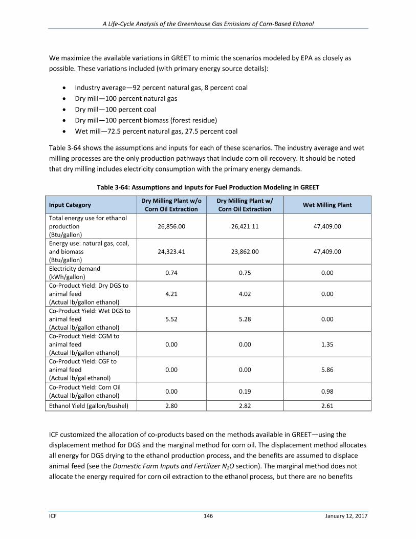
A Life-Cycle Analysis of the Greenhouse Gas Emissions of Corn-Based Ethanol
ICF 146 January 12, 2017
We maximize the available variations in GREET to mimic the scenarios modeled by EPA as closely as
possible. These variations included (with primary energy source details):
Industry average—92 percent natural gas, 8 percent coal
Dry mill—100 percent natural gas
Dry mill—100 percent coal
Dry mill—100 percent biomass (forest residue)
Wet mill—72.5 percent natural gas, 27.5 percent coal
Table 3-64 shows the assumptions and inputs for each of these scenarios. The industry average and wet
milling processes are the only production pathways that include corn oil recovery. It should be noted
that dry milling includes electricity consumption with the primary energy demands.
Table 3-64: Assumptions and Inputs for Fuel Production Modeling in GREET
Input Category Dry Milling Plant w/o
Corn Oil Extraction Dry Milling Plant w/ Corn Oil Extraction
Wet Milling Plant
Total energy use for ethanol production (Btu/gallon)
26,856.00 26,421.11 47,409.00
Energy use: natural gas, coal, and biomass (Btu/gallon)
24,323.41 23,862.00 47,409.00
Electricity demand (kWh/gallon)
0.74 0.75 0.00
Co-Product Yield: Dry DGS to animal feed (Actual lb/gallon ethanol)
4.21 4.02 0.00
Co-Product Yield: Wet DGS to animal feed (Actual lb/gallon ethanol)
5.52 5.28 0.00
Co-Product Yield: CGM to animal feed (Actual lb/gallon ethanol)
0.00 0.00 1.35
Co-Product Yield: CGF to animal feed (Actual lb/gal ethanol)
0.00 0.00 5.86
Co-Product Yield: Corn Oil (Actual lb/gallon ethanol)
0.00 0.19 0.98
Ethanol Yield (gallon/bushel) 2.80 2.82 2.61
ICF customized the allocation of co-products based on the methods available in GREET—using the
displacement method for DGS and the marginal method for corn oil. The displacement method allocates
all energy for DGS drying to the ethanol production process, and the benefits are assumed to displace
animal feed (see the Domestic Farm Inputs and Fertilizer N2O section). The marginal method does not
allocate the energy required for corn oil extraction to the ethanol process, but there are no benefits
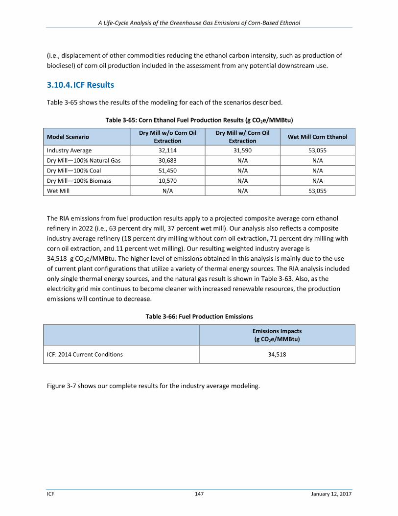
A Life-Cycle Analysis of the Greenhouse Gas Emissions of Corn-Based Ethanol
ICF 147 January 12, 2017
(i.e., displacement of other commodities reducing the ethanol carbon intensity, such as production of
biodiesel) of corn oil production included in the assessment from any potential downstream use.
3.10.4. ICF Results
Table 3-65 shows the results of the modeling for each of the scenarios described.
Table 3-65: Corn Ethanol Fuel Production Results (g CO2e/MMBtu)
Model Scenario Dry Mill w/o Corn Oil
Extraction Dry Mill w/ Corn Oil
Extraction Wet Mill Corn Ethanol
Industry Average 32,114 31,590 53,055
Dry Mill—100% Natural Gas 30,683 N/A N/A
Dry Mill—100% Coal 51,450 N/A N/A
Dry Mill—100% Biomass 10,570 N/A N/A
Wet Mill N/A N/A 53,055
The RIA emissions from fuel production results apply to a projected composite average corn ethanol
refinery in 2022 (i.e., 63 percent dry mill, 37 percent wet mill). Our analysis also reflects a composite
industry average refinery (18 percent dry milling without corn oil extraction, 71 percent dry milling with
corn oil extraction, and 11 percent wet milling). Our resulting weighted industry average is
34,518 g CO2e/MMBtu. The higher level of emissions obtained in this analysis is mainly due to the use
of current plant configurations that utilize a variety of thermal energy sources. The RIA analysis included
only single thermal energy sources, and the natural gas result is shown in Table 3-63. Also, as the
electricity grid mix continues to become cleaner with increased renewable resources, the production
emissions will continue to decrease.
Table 3-66: Fuel Production Emissions
Emissions Impacts (g CO2e/MMBtu)
ICF: 2014 Current Conditions 34,518
Figure 3-7 shows our complete results for the industry average modeling.
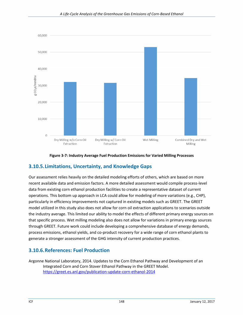
A Life-Cycle Analysis of the Greenhouse Gas Emissions of Corn-Based Ethanol
ICF 148 January 12, 2017
Figure 3-7: Industry Average Fuel Production Emissions for Varied Milling Processes
3.10.5. Limitations, Uncertainty, and Knowledge Gaps
Our assessment relies heavily on the detailed modeling efforts of others, which are based on more
recent available data and emission factors. A more detailed assessment would compile process-level
data from existing corn ethanol production facilities to create a representative dataset of current
operations. This bottom up approach in LCA could allow for modeling of more variations (e.g., CHP),
particularly in efficiency improvements not captured in existing models such as GREET. The GREET
model utilized in this study also does not allow for corn oil extraction applications to scenarios outside
the industry average. This limited our ability to model the effects of different primary energy sources on
that specific process. Wet milling modeling also does not allow for variations in primary energy sources
through GREET. Future work could include developing a comprehensive database of energy demands,
process emissions, ethanol yields, and co-product recovery for a wide range of corn ethanol plants to
generate a stronger assessment of the GHG intensity of current production practices.
3.10.6. References: Fuel Production
Argonne National Laboratory, 2014. Updates to the Corn Ethanol Pathway and Development of an Integrated Corn and Corn Stover Ethanol Pathway in the GREET Model. https://greet.es.anl.gov/publication-update-corn-ethanol-2014
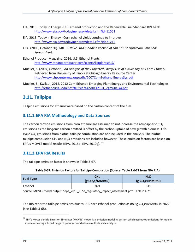
A Life-Cycle Analysis of the Greenhouse Gas Emissions of Corn-Based Ethanol
ICF 149 January 12, 2017
EIA, 2013. Today in Energy - U.S. ethanol production and the Renewable Fuel Standard RIN bank. http://www.eia.gov/todayinenergy/detail.cfm?id=11551
EIA, 2015. Today in Energy - Corn ethanol yields continue to improve. http://www.eia.gov/todayinenergy/detail.cfm?id=21212
EPA. (2009, October 30). GREET. RFS2 FRM modified version of GREET1.8c Upstream Emissions Spreadsheet.
Ethanol Producer Magazine, 2016. U.S. Ethanol Plants. http://www.ethanolproducer.com/plants/listplants/US/
Mueller, S. (2007, October ). An Analysis of the Projected Energy Use of Future Dry Mill Corn Ethanol. Retrieved from University of Illinois at Chicago Energy Resource Center: http://www.chpcentermw.org/pdfs/2007CornEethanolEnergySys.pdf
Mueller, S., Kwik, J., 2012. 2012 Corn Ethanol: Emerging Plant Energy and Environmental Technologies. http://ethanolrfa.3cdn.net/fe5f4b7a4bdbc12101_2gm6bejk4.pdf
3.11. Tailpipe
Tailpipe emissions for ethanol were based on the carbon content of the fuel.
3.11.1. EPA RIA Methodology and Data Sources
The carbon dioxide emissions from corn ethanol are assumed to not increase the atmospheric CO2
emissions as the biogenic carbon emitted is offset by the carbon uptake of new growth biomass. Life-
cycle CO2 emissions from biofuel tailpipe combustion are not included in the analysis. The biofuel
tailpipe combustion CH4 and N2O emissions are included however. These emission factors are based on
EPA’s MOVES model results (EPA, 2015b; EPA, 2010g). 32
3.11.2. EPA RIA Results
The tailpipe emission factor is shown in Table 3-67.
Table 3-67: Emission Factors for Tailpipe Combustion (Source: Table 2.4-71 from EPA RIA)
Fuel Type CH4
(g CO2e/MMBtu) N2O
(g CO2e/MMBtu)
Ethanol 269 611
Source: MOVES model output; “epa_2010_RFS2_regulatory_impact_assessment.pdf” Table 2.4-71.
The RIA reported tailpipe emissions due to U.S. corn ethanol production as 880 g CO2e/MMBtu in 2022
(see Table 3-68).
32 EPA’s Motor Vehicle Emission Simulator (MOVES) model is a emission modeling system which estimates emissions for mobile
sources covering a broad range of pollutants and allows multiple scale analysis.
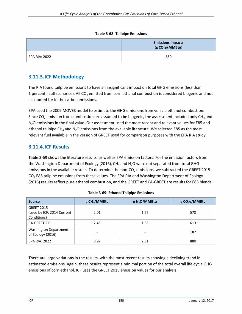
A Life-Cycle Analysis of the Greenhouse Gas Emissions of Corn-Based Ethanol
ICF 150 January 12, 2017
Table 3-68: Tailpipe Emissions
Emissions Impacts (g CO2e/MMBtu)
EPA RIA: 2022 880
3.11.3. ICF Methodology
The RIA found tailpipe emissions to have an insignificant impact on total GHG emissions (less than
1 percent in all scenarios). All CO2 emitted from corn ethanol combustion is considered biogenic and not
accounted for in the carbon emissions.
EPA used the 2009 MOVES model to estimate the GHG emissions from vehicle ethanol combustion.
Since CO2 emission from combustion are assumed to be biogenic, the assessment included only CH4 and
N2O emissions in the final value. Our assessment used the most recent and relevant values for E85 and
ethanol tailpipe CH4 and N2O emissions from the available literature. We selected E85 as the most
relevant fuel available in the version of GREET used for comparison purposes with the EPA RIA study.
3.11.4. ICF Results
Table 3-69 shows the literature results, as well as EPA emission factors. For the emission factors from
the Washington Department of Ecology (2016), CH4 and N2O were not separated from total GHG
emissions in the available results. To determine the non-CO2 emissions, we subtracted the GREET 2015
CO2 E85 tailpipe emissions from these values. The EPA RIA and Washington Department of Ecology
(2016) results reflect pure ethanol combustion, and the GREET and CA-GREET are results for E85 blends.
Table 3-69: Ethanol Tailpipe Emissions
Source g CH4/MMBtu g N2O/MMBtu g CO2e/MMBtu
GREET 2015 (used by ICF: 2014 Current Conditions)
2.01 1.77 578
CA-GREET 2.0 2.45 1.85 613
Washington Department of Ecology (2016)
- - 187
EPA RIA: 2022 8.97 2.31 880
There are large variations in the results, with the most recent results showing a declining trend in
estimated emissions. Again, these results represent a minimal portion of the total overall life-cycle GHG
emissions of corn ethanol. ICF uses the GREET 2015 emission values for our analysis.
A Life-Cycle Analysis of the Greenhouse Gas Emissions of Corn-Based Ethanol
ICF 151 January 12, 2017
3.11.5. Limitations, Uncertainty, and Knowledge Gaps
The EPA RIA used the 2009 MOVES model to estimate the GHG emissions from vehicle ethanol
combustion. Our analysis did not use the more recent (2015) EPA MOVES model for determining ethanol
emissions. MOVES is the official model for state implementation plans (SIPs) and transportation
conformity, as well as being the standard for determining tailpipe GHG emissions. MOVES bases
emissions on instantaneous energy consumption and a continually-updated database to generate
emission factors customized for regional, temporal, and other scenarios. Because of this highly-region-
specific nature of MOVES, this study instead used recent literature that focused on average emission
factors. Future assessments could utilize the latest version of MOVES to better estimate ethanol tailpipe
emissions. However, this added effort will likely have a minimal effect on the overall accuracy of the
corn ethanol LCA, as tailpipe emissions are comparatively less significant.
3.11.6. References: Tailpipe
California ARB, 2015. CA-GREET 2.0 Model. http://www.arb.ca.gov/fuels/lcfs/ca-greet/ca-greet.htm
EPA. (2010g). NMIM and MOVES Runs for RFS2 Air Quality Modeling: Memorandum.
EPA. (2015b, October 13). Motor Vehicle Emission Simulator). Retrieved from http://www.epa.gov/otaq/models/moves/index.htm
Washington Department of Ecology, 2016. Greenhouse Gas Reporting: Transportation Fuel Suppliers. http://www.ecy.wa.gov/programs/air/permit_register/ghg/GHG_transp.html
3.12. Result of Combining the Current GHG Emission Category Values
This section presents a current GHG LCA for corn ethanol production. The data used to develop this LCA
span the 2010–2014 timeframe and, consequently, the ICF: 2014 Current Conditions analysis is
appropriately viewed as the current GHG profile of corn ethanol. The EPA RIA LCA was a projection,
done in 2010, of GHG emissions from a new natural gas powered ethanol refinery in 2022. The RIA and
ICF LCAs are directly comparable because the large majority of existing refineries use natural gas (i.e.,
the industry has already shifted away from coal-fired plants) and industry ethanol production, that is
13.5–14.5 billion gallons a year, is very close to the 15 billion gallon cap in the RFS2.
Figure 3-8 shows the results of combining the 11 emission categories from the EPA RIA: 2022 and ICF:
2014 Current Conditions analyses.
The EPA RIA: 2022 LCA value for corn ethanol is 79,180 g CO2e/MMBtu compared to
98,000 g CO2e/MMBtu for the 2005 gasoline baseline which is used as the fossil fuel carbon intensity
reference in the RFS2.
Our ICF: 2014 Current Conditions value is 55,731 g CO2e/MMBtu.
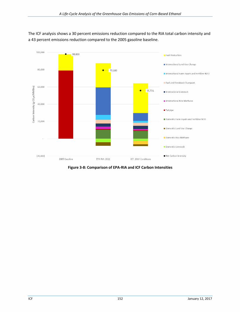
A Life-Cycle Analysis of the Greenhouse Gas Emissions of Corn-Based Ethanol
ICF 152 January 12, 2017
The ICF analysis shows a 30 percent emissions reduction compared to the RIA total carbon intensity and
a 43 percent emissions reduction compared to the 2005 gasoline baseline.
Figure 3-8: Comparison of EPA-RIA and ICF Carbon Intensities
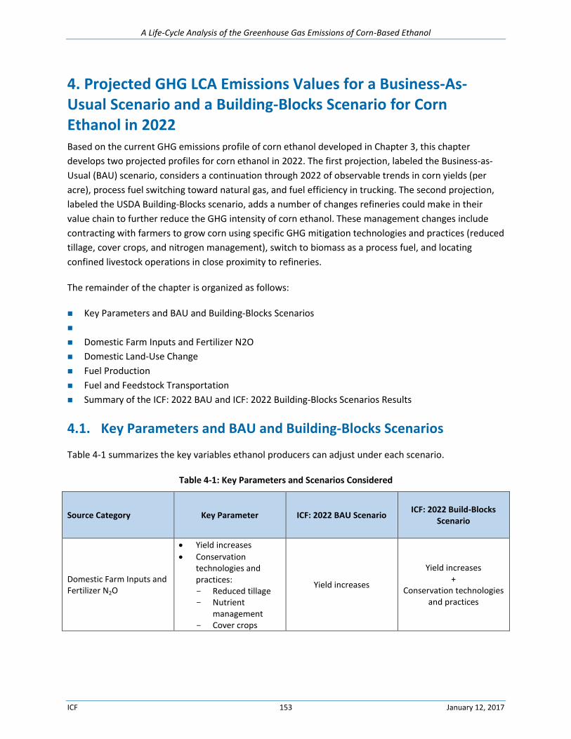
A Life-Cycle Analysis of the Greenhouse Gas Emissions of Corn-Based Ethanol
ICF 153 January 12, 2017
4. Projected GHG LCA Emissions Values for a Business-As-Usual Scenario and a Building-Blocks Scenario for Corn Ethanol in 2022 Based on the current GHG emissions profile of corn ethanol developed in Chapter 3, this chapter
develops two projected profiles for corn ethanol in 2022. The first projection, labeled the Business-as-
Usual (BAU) scenario, considers a continuation through 2022 of observable trends in corn yields (per
acre), process fuel switching toward natural gas, and fuel efficiency in trucking. The second projection,
labeled the USDA Building-Blocks scenario, adds a number of changes refineries could make in their
value chain to further reduce the GHG intensity of corn ethanol. These management changes include
contracting with farmers to grow corn using specific GHG mitigation technologies and practices (reduced
tillage, cover crops, and nitrogen management), switch to biomass as a process fuel, and locating
confined livestock operations in close proximity to refineries.
The remainder of the chapter is organized as follows:
Key Parameters and BAU and Building-Blocks Scenarios
Domestic Farm Inputs and Fertilizer N2O
Domestic Land-Use Change
Fuel Production
Fuel and Feedstock Transportation
Summary of the ICF: 2022 BAU and ICF: 2022 Building-Blocks Scenarios Results
4.1. Key Parameters and BAU and Building-Blocks Scenarios
Table 4-1 summarizes the key variables ethanol producers can adjust under each scenario.
Table 4-1: Key Parameters and Scenarios Considered
Source Category Key Parameter ICF: 2022 BAU Scenario ICF: 2022 Build-Blocks
Scenario
Domestic Farm Inputs and Fertilizer N2O
Yield increases
Conservation technologies and practices: Reduced tillage Nutrient
management Cover crops
Yield increases
Yield increases +
Conservation technologies and practices
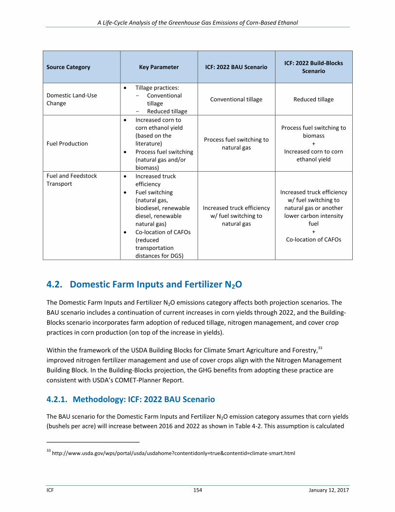
A Life-Cycle Analysis of the Greenhouse Gas Emissions of Corn-Based Ethanol
ICF 154 January 12, 2017
Source Category Key Parameter ICF: 2022 BAU Scenario ICF: 2022 Build-Blocks
Scenario
Domestic Land-Use Change
Tillage practices: Conventional
tillage Reduced tillage
Conventional tillage Reduced tillage
Fuel Production
Increased corn to corn ethanol yield (based on the literature)
Process fuel switching (natural gas and/or biomass)
Process fuel switching to natural gas
Process fuel switching to biomass
+ Increased corn to corn
ethanol yield
Fuel and Feedstock Transport
Increased truck efficiency
Fuel switching (natural gas, biodiesel, renewable diesel, renewable natural gas)
Co-location of CAFOs (reduced transportation distances for DGS)
Increased truck efficiency w/ fuel switching to
natural gas
Increased truck efficiency w/ fuel switching to
natural gas or another lower carbon intensity
fuel +
Co-location of CAFOs
4.2. Domestic Farm Inputs and Fertilizer N2O
The Domestic Farm Inputs and Fertilizer N2O emissions category affects both projection scenarios. The
BAU scenario includes a continuation of current increases in corn yields through 2022, and the Building-
Blocks scenario incorporates farm adoption of reduced tillage, nitrogen management, and cover crop
practices in corn production (on top of the increase in yields).
Within the framework of the USDA Building Blocks for Climate Smart Agriculture and Forestry,33
improved nitrogen fertilizer management and use of cover crops align with the Nitrogen Management
Building Block. In the Building-Blocks projection, the GHG benefits from adopting these practice are
consistent with USDA’s COMET-Planner Report.
4.2.1. Methodology: ICF: 2022 BAU Scenario
The BAU scenario for the Domestic Farm Inputs and Fertilizer N2O emission category assumes that corn yields
(bushels per acre) will increase between 2016 and 2022 as shown in Table 4-2. This assumption is calculated
33 http://www.usda.gov/wps/portal/usda/usdahome?contentidonly=true&contentid=climate-smart.html
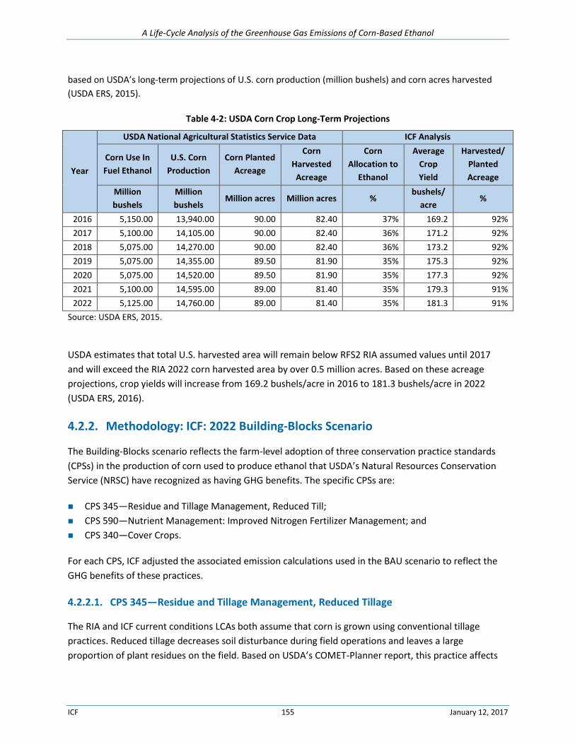
A Life-Cycle Analysis of the Greenhouse Gas Emissions of Corn-Based Ethanol
ICF 155 January 12, 2017
based on USDA’s long-term projections of U.S. corn production (million bushels) and corn acres harvested
(USDA ERS, 2015).
Table 4-2: USDA Corn Crop Long-Term Projections
Year
USDA National Agricultural Statistics Service Data ICF Analysis
Corn Use In
Fuel Ethanol
U.S. Corn
Production
Corn Planted
Acreage
Corn
Harvested
Acreage
Corn
Allocation to
Ethanol
Average
Crop
Yield
Harvested/
Planted
Acreage
Million
bushels
Million
bushels Million acres Million acres %
bushels/
acre %
2016 5,150.00 13,940.00 90.00 82.40 37% 169.2 92%
2017 5,100.00 14,105.00 90.00 82.40 36% 171.2 92%
2018 5,075.00 14,270.00 90.00 82.40 36% 173.2 92%
2019 5,075.00 14,355.00 89.50 81.90 35% 175.3 92%
2020 5,075.00 14,520.00 89.50 81.90 35% 177.3 92%
2021 5,100.00 14,595.00 89.00 81.40 35% 179.3 91%
2022 5,125.00 14,760.00 89.00 81.40 35% 181.3 91%
Source: USDA ERS, 2015.
USDA estimates that total U.S. harvested area will remain below RFS2 RIA assumed values until 2017
and will exceed the RIA 2022 corn harvested area by over 0.5 million acres. Based on these acreage
projections, crop yields will increase from 169.2 bushels/acre in 2016 to 181.3 bushels/acre in 2022
(USDA ERS, 2016).
4.2.2. Methodology: ICF: 2022 Building-Blocks Scenario
The Building-Blocks scenario reflects the farm-level adoption of three conservation practice standards
(CPSs) in the production of corn used to produce ethanol that USDA’s Natural Resources Conservation
Service (NRSC) have recognized as having GHG benefits. The specific CPSs are:
CPS 345—Residue and Tillage Management, Reduced Till;
CPS 590—Nutrient Management: Improved Nitrogen Fertilizer Management; and
CPS 340—Cover Crops.
For each CPS, ICF adjusted the associated emission calculations used in the BAU scenario to reflect the
GHG benefits of these practices.
4.2.2.1. CPS 345—Residue and Tillage Management, Reduced Tillage
The RIA and ICF current conditions LCAs both assume that corn is grown using conventional tillage
practices. Reduced tillage decreases soil disturbance during field operations and leaves a large
proportion of plant residues on the field. Based on USDA’s COMET-Planner report, this practice affects
A Life-Cycle Analysis of the Greenhouse Gas Emissions of Corn-Based Ethanol
ICF 156 January 12, 2017
the soil carbon storage (see Domestic Land-Use Change section below) and nitrous oxide emissions from
changes in the soil environment. It does not affect any changes in fertilizer application rates.
To account for the adoption of reduced tillage in this analysis, ICF adjusted the fuel used for on-farm
equipment and reduced the indirect N2O emissions associated with conventional tillage. Diesel fuel use
is assumed to be 7.74 gallons per corn-acre under conventional tillage, based on 2015 farm budget
worksheets published by the University of Tennessee (2015). To model reduced tillage, ICF reduced the
fuel used for chisel and disk machinery in the conventional tillage case by 50 percent. Fuel use and
related CO2 emissions for all other equipment used in no-till systems remained the same as in
conventional tillage systems (University of Tennessee, 2015). This resulted in a fuel consumption of
6.95 gallons per corn-acre. With respect to indirect N2O emissions, the shift from conventional to
reduced tillage reduces the volatization rate of nitrogen fertilizer (Swan et al., n.d.) The COMET-Planner
report attributes a 0.07 Mg CO2e/acre/year reduction in emissions due to reduced tillage relative to
conventional tillage. This represents a 74.4 percent reduction in volatization N2O emissions (here
measured in kg N2O/acre per kilogram of nitrogen applied).
4.2.2.2. CPS 590—Nutrient Management: Improved Nitrogen Fertilizer Management
CPS 590 assumes the adoption of new nitrogen fertilizer management techniques including reduced
application rates from targeted nitrogen fertilizer application management and the use of nitrification
inhibitors. The COMET-Planner report estimates that CPS 590 practices can reduce nitrogen application
rates by 15 percent. This percent adjustment was made to the application rates in the Building-Blocks
scenario.
Nitrification inhibitors are applied to reduce the leaching or production of N2O in the soil. The most
common nitrification inhibitor used in the United States on corn acres is nitrapyrin. A report by the
International Fertilizer Industry Association states that application rates of nitrapyrin range between
1.4–5.6 liters per hectare (Trenkel 2010). The assumed density is 1.582 grams/cm3 (LookChem 2008).
Based on these data, ICF assumed an application rate of 2.24 kg/acre. There are very few sources of
publically available life-cycle assessment data with which to quantify the upstream emissions for
nitrification inhibitors. For the upstream production emissions, ICF used “Organophosphorus-
compound” from the ecoinvent database (Weidema et al. 2013) as a proxy for nitrapyrin. The emissions
per kilogram of product are in line with those found in Dow’s “Using LCA to Identify Options for
Greenhouse Gas Emission Reductions in Australian Wheat Farming" (Helling et al. 2014).
4.2.2.3. CPS 340—Cover Crops
Cover crops are planted in addition to seasonal crops to increase the nitrogen and water-use
efficiencies. The additional crop residues increase soil carbon levels (Swan et al., n.d.) and can reduce
the indirect emissions of nitrogen (e.g., N2O). The reductions of indirect N2O emissions are due to
decreases in the leaching rate of nitrogen fertilizer (Swan et al., n.d.). The COMET-Planner report
attributes a 0.05 Mg CO2e/acre/year reduction in emissions due to cover crops. This represents a
76.8 percent reduction in leaching N2O emissions (here measured in kg N2O/acre per kilogram of
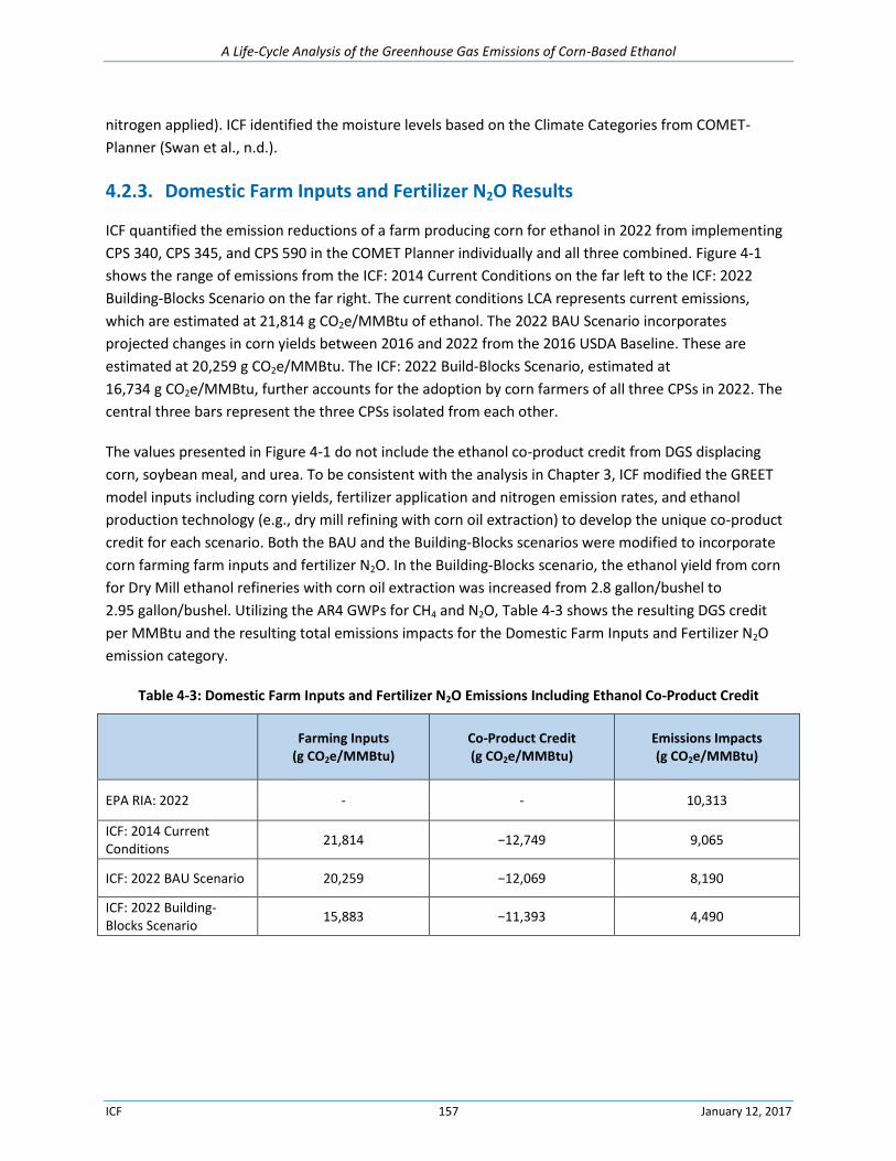
A Life-Cycle Analysis of the Greenhouse Gas Emissions of Corn-Based Ethanol
ICF 157 January 12, 2017
nitrogen applied). ICF identified the moisture levels based on the Climate Categories from COMET-
Planner (Swan et al., n.d.).
4.2.3. Domestic Farm Inputs and Fertilizer N2O Results
ICF quantified the emission reductions of a farm producing corn for ethanol in 2022 from implementing
CPS 340, CPS 345, and CPS 590 in the COMET Planner individually and all three combined. Figure 4-1
shows the range of emissions from the ICF: 2014 Current Conditions on the far left to the ICF: 2022
Building-Blocks Scenario on the far right. The current conditions LCA represents current emissions,
which are estimated at 21,814 g CO2e/MMBtu of ethanol. The 2022 BAU Scenario incorporates
projected changes in corn yields between 2016 and 2022 from the 2016 USDA Baseline. These are
estimated at 20,259 g CO2e/MMBtu. The ICF: 2022 Build-Blocks Scenario, estimated at
16,734 g CO2e/MMBtu, further accounts for the adoption by corn farmers of all three CPSs in 2022. The
central three bars represent the three CPSs isolated from each other.
The values presented in Figure 4-1 do not include the ethanol co-product credit from DGS displacing
corn, soybean meal, and urea. To be consistent with the analysis in Chapter 3, ICF modified the GREET
model inputs including corn yields, fertilizer application and nitrogen emission rates, and ethanol
production technology (e.g., dry mill refining with corn oil extraction) to develop the unique co-product
credit for each scenario. Both the BAU and the Building-Blocks scenarios were modified to incorporate
corn farming farm inputs and fertilizer N2O. In the Building-Blocks scenario, the ethanol yield from corn
for Dry Mill ethanol refineries with corn oil extraction was increased from 2.8 gallon/bushel to
2.95 gallon/bushel. Utilizing the AR4 GWPs for CH4 and N2O, Table 4-3 shows the resulting DGS credit
per MMBtu and the resulting total emissions impacts for the Domestic Farm Inputs and Fertilizer N2O
emission category.
Table 4-3: Domestic Farm Inputs and Fertilizer N2O Emissions Including Ethanol Co-Product Credit
Farming Inputs
(g CO2e/MMBtu) Co-Product Credit (g CO2e/MMBtu)
Emissions Impacts (g CO2e/MMBtu)
EPA RIA: 2022 - - 10,313
ICF: 2014 Current Conditions
21,814 −12,749 9,065
ICF: 2022 BAU Scenario 20,259 −12,069 8,190
ICF: 2022 Building-Blocks Scenario
15,883 −11,393 4,490
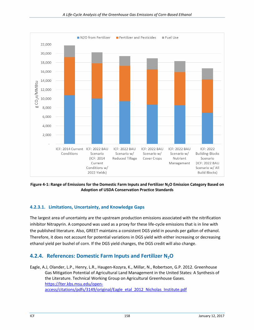
A Life-Cycle Analysis of the Greenhouse Gas Emissions of Corn-Based Ethanol
ICF 158 January 12, 2017
Figure 4-1: Range of Emissions for the Domestic Farm Inputs and Fertilizer N2O Emission Category Based on Adoption of USDA Conservation Practice Standards
4.2.3.1. Limitations, Uncertainty, and Knowledge Gaps
The largest area of uncertainty are the upstream production emissions associated with the nitrification
inhibitor Nitrapyrin. A compound was used as a proxy for these life-cycle emissions that is in line with
the published literature. Also, GREET maintains a consistent DGS yield in pounds per gallon of ethanol.
Therefore, it does not account for potential variations in DGS yield with either increasing or decreasing
ethanol yield per bushel of corn. If the DGS yield changes, the DGS credit will also change.
4.2.4. References: Domestic Farm Inputs and Fertilizer N2O
Eagle, A.J, Olander, L.P., Henry, L.R., Haugen-Kozyra, K., Millar, N., Robertson, G.P. 2012. Greenhouse Gas Mitigation Potential of Agricultural Land Management in the United States: A Synthesis of the Literature. Technical Working Group on Agricultural Greenhouse Gases. https://lter.kbs.msu.edu/open-access/citations/pdfs/3149/original/Eagle_etal_2012_Nicholas_Institute.pdf
A Life-Cycle Analysis of the Greenhouse Gas Emissions of Corn-Based Ethanol
ICF 159 January 12, 2017
Helling, R.K., Cass, I., Merrill, J. 2014. Using LCA to Identify Options for Greenhouse Gas Emission Reductions in Australian Wheat Farming. Proceedings of the 9th International Conference on Life Cycle Assessment in the Agri-Food Sector. http://lcafood2014.org/papers/280.pdf
LookChem. 2008. Nitrapyrin. http://www.lookchem.com/Nitrapyrin/
Trenkel, M.E. 2010. Slow- and Controlled-Release and Stabilized Fertilizers: An Option for Enhancing Nutrient Use Efficiency in Agriculture. International Fertilizer Industry Association.
Swan, A., Williams, S.A., Brown, K., Chambers, A., Creque, J., Wick, J., Paustian, K. COMET-PLANNER: Carbon and greenhouse gas evaluation for NRCS conservation practice planning. http://www.comet-planner.com/
University of Tennessee. 2015. Field Crop Budgets For 2015 E12-4115: University of Tennessee Institute of Agriculture. http://economics.ag.utk.edu/budgets/2015/Crops/2015CropBudgets.pdf
USDA. 2016. USDA Agricultural Projections to 2025. USDA Agricultural Projections No. (OCE-2016-1) 99 pp, February 2016. http://www.ers.usda.gov/publications/oce-usda-agricultural-projections/oce-2016-1.aspx
Weidema, B.P., C. Bauer, R. Hischier, C. Mutel, et al. 2013. The ecoinvent database: Overview and methodology, Data quality guideline for the ecoinvent database version 3. www.ecoinvent.org
4.3. Domestic Land-Use Change
The BAU and Building-Blocks scenarios incorporate projections to 2022 for the following key variable
that affects GHG emissions under the Domestic Land-Use Change source category:
Continuation of conventional till practices by farms for producing corn for ethanol; versus
Adoption of reduced till practices by farms producing corn for ethanol.
4.3.1. Methodology
The methodology and results for determining total acreage change and emission factors can be found in
the Chapter 3 (see Section 3.1.7). This assessment used the same emission factors and anticipated
acreage changes as the ICF current conditions LCA. Acreage changes are based on the 2013 corn ethanol
production scenario in the GREET model’s Carbon Calculator for Land Use Change from Biofuels
Production (CCLUB) (Dunn et al., 2015). Using the 2013 production scenario assumes that total U.S. corn
ethanol production will remain constant at 15 billion gallons annually through 2022 (11.59 billion
gallons/year greater than 2004 production levels). The difference between the BAU scenario and Build-
Blocks scenario is the continued adoption of conventional till in the BAU scenario and the adoption of
reduced till in the Building-Blocks scenario.
4.3.2. Domestic Land-Use Change Results
Table 4-4 shows the total GHG emission results for conventional (ICF: 2022 BAU Scenario) and reduced
till (ICF: 2022 Build-Blocks Scenario) for 100 cm soil depths.
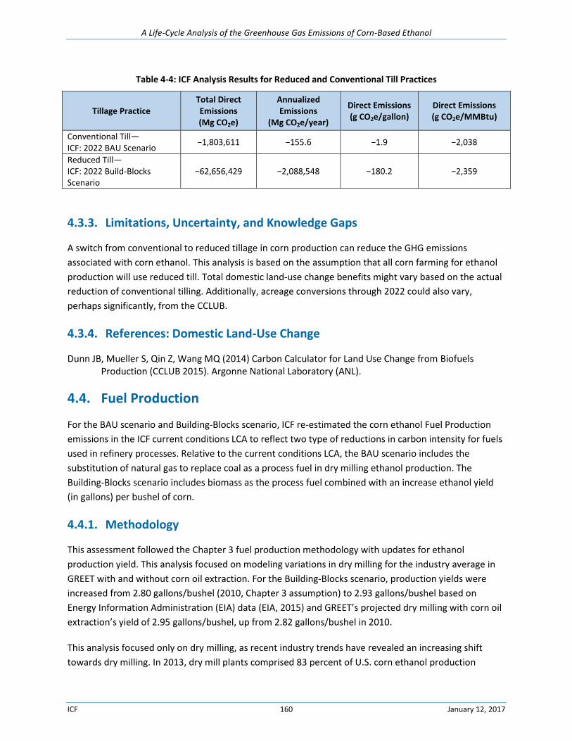
A Life-Cycle Analysis of the Greenhouse Gas Emissions of Corn-Based Ethanol
ICF 160 January 12, 2017
Table 4-4: ICF Analysis Results for Reduced and Conventional Till Practices
Tillage Practice Total Direct Emissions (Mg CO2e)
Annualized Emissions
(Mg CO2e/year)
Direct Emissions (g CO2e/gallon)
Direct Emissions (g CO2e/MMBtu)
Conventional Till— ICF: 2022 BAU Scenario
−1,803,611 −155.6 −1.9 −2,038
Reduced Till— ICF: 2022 Build-Blocks Scenario
−62,656,429 −2,088,548 −180.2 −2,359
4.3.3. Limitations, Uncertainty, and Knowledge Gaps
A switch from conventional to reduced tillage in corn production can reduce the GHG emissions
associated with corn ethanol. This analysis is based on the assumption that all corn farming for ethanol
production will use reduced till. Total domestic land-use change benefits might vary based on the actual
reduction of conventional tilling. Additionally, acreage conversions through 2022 could also vary,
perhaps significantly, from the CCLUB.
4.3.4. References: Domestic Land-Use Change
Dunn JB, Mueller S, Qin Z, Wang MQ (2014) Carbon Calculator for Land Use Change from Biofuels Production (CCLUB 2015). Argonne National Laboratory (ANL).
4.4. Fuel Production
For the BAU scenario and Building-Blocks scenario, ICF re-estimated the corn ethanol Fuel Production
emissions in the ICF current conditions LCA to reflect two type of reductions in carbon intensity for fuels
used in refinery processes. Relative to the current conditions LCA, the BAU scenario includes the
substitution of natural gas to replace coal as a process fuel in dry milling ethanol production. The
Building-Blocks scenario includes biomass as the process fuel combined with an increase ethanol yield
(in gallons) per bushel of corn.
4.4.1. Methodology
This assessment followed the Chapter 3 fuel production methodology with updates for ethanol
production yield. This analysis focused on modeling variations in dry milling for the industry average in
GREET with and without corn oil extraction. For the Building-Blocks scenario, production yields were
increased from 2.80 gallons/bushel (2010, Chapter 3 assumption) to 2.93 gallons/bushel based on
Energy Information Administration (EIA) data (EIA, 2015) and GREET’s projected dry milling with corn oil
extraction’s yield of 2.95 gallons/bushel, up from 2.82 gallons/bushel in 2010.
This analysis focused only on dry milling, as recent industry trends have revealed an increasing shift
towards dry milling. In 2013, dry mill plants comprised 83 percent of U.S. corn ethanol production
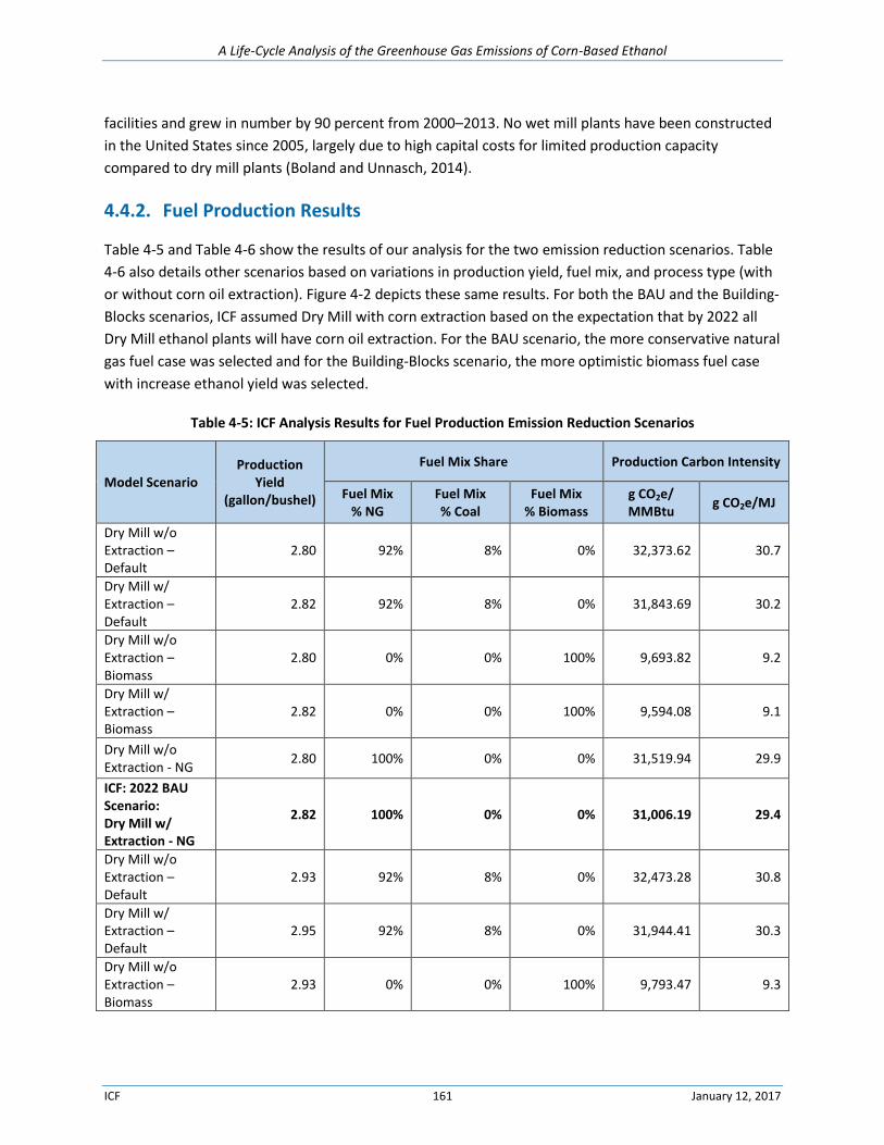
A Life-Cycle Analysis of the Greenhouse Gas Emissions of Corn-Based Ethanol
ICF 161 January 12, 2017
facilities and grew in number by 90 percent from 2000–2013. No wet mill plants have been constructed
in the United States since 2005, largely due to high capital costs for limited production capacity
compared to dry mill plants (Boland and Unnasch, 2014).
4.4.2. Fuel Production Results
Table 4-5 and Table 4-6 show the results of our analysis for the two emission reduction scenarios. Table
4-6 also details other scenarios based on variations in production yield, fuel mix, and process type (with
or without corn oil extraction). Figure 4-2 depicts these same results. For both the BAU and the Building-
Blocks scenarios, ICF assumed Dry Mill with corn extraction based on the expectation that by 2022 all
Dry Mill ethanol plants will have corn oil extraction. For the BAU scenario, the more conservative natural
gas fuel case was selected and for the Building-Blocks scenario, the more optimistic biomass fuel case
with increase ethanol yield was selected.
Table 4-5: ICF Analysis Results for Fuel Production Emission Reduction Scenarios
Model Scenario
Production Yield
(gallon/bushel)
Fuel Mix Share Production Carbon Intensity
Fuel Mix % NG
Fuel Mix % Coal
Fuel Mix % Biomass
g CO2e/ MMBtu
g CO2e/MJ
Dry Mill w/o Extraction – Default
2.80 92% 8% 0% 32,373.62 30.7
Dry Mill w/ Extraction – Default
2.82 92% 8% 0% 31,843.69 30.2
Dry Mill w/o Extraction – Biomass
2.80 0% 0% 100% 9,693.82 9.2
Dry Mill w/ Extraction – Biomass
2.82 0% 0% 100% 9,594.08 9.1
Dry Mill w/o Extraction - NG
2.80 100% 0% 0% 31,519.94 29.9
ICF: 2022 BAU Scenario: Dry Mill w/ Extraction - NG
2.82 100% 0% 0% 31,006.19 29.4
Dry Mill w/o Extraction – Default
2.93 92% 8% 0% 32,473.28 30.8
Dry Mill w/ Extraction – Default
2.95 92% 8% 0% 31,944.41 30.3
Dry Mill w/o Extraction – Biomass
2.93 0% 0% 100% 9,793.47 9.3
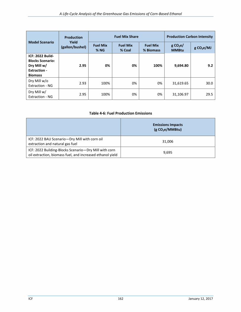
A Life-Cycle Analysis of the Greenhouse Gas Emissions of Corn-Based Ethanol
ICF 162 January 12, 2017
Model Scenario
Production Yield
(gallon/bushel)
Fuel Mix Share Production Carbon Intensity
Fuel Mix % NG
Fuel Mix % Coal
Fuel Mix % Biomass
g CO2e/ MMBtu
g CO2e/MJ
ICF: 2022 Build-Blocks Scenario: Dry Mill w/ Extraction - Biomass
2.95 0% 0% 100% 9,694.80 9.2
Dry Mill w/o Extraction - NG
2.93 100% 0% 0% 31,619.65 30.0
Dry Mill w/ Extraction - NG
2.95 100% 0% 0% 31,106.97 29.5
Table 4-6: Fuel Production Emissions
Emissions Impacts (g CO2e/MMBtu)
ICF: 2022 BAU Scenario—Dry Mill with corn oil extraction and natural gas fuel
31,006
ICF: 2022 Building-Blocks Scenario—Dry Mill with corn oil extraction, biomass fuel, and increased ethanol yield
9,695
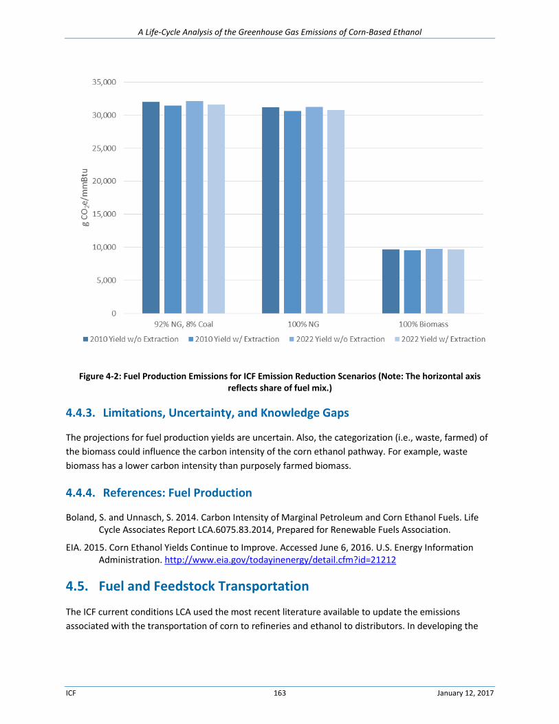
A Life-Cycle Analysis of the Greenhouse Gas Emissions of Corn-Based Ethanol
ICF 163 January 12, 2017
Figure 4-2: Fuel Production Emissions for ICF Emission Reduction Scenarios (Note: The horizontal axis reflects share of fuel mix.)
4.4.3. Limitations, Uncertainty, and Knowledge Gaps
The projections for fuel production yields are uncertain. Also, the categorization (i.e., waste, farmed) of
the biomass could influence the carbon intensity of the corn ethanol pathway. For example, waste
biomass has a lower carbon intensity than purposely farmed biomass.
4.4.4. References: Fuel Production
Boland, S. and Unnasch, S. 2014. Carbon Intensity of Marginal Petroleum and Corn Ethanol Fuels. Life Cycle Associates Report LCA.6075.83.2014, Prepared for Renewable Fuels Association.
EIA. 2015. Corn Ethanol Yields Continue to Improve. Accessed June 6, 2016. U.S. Energy Information Administration. http://www.eia.gov/todayinenergy/detail.cfm?id=21212
4.5. Fuel and Feedstock Transportation
The ICF current conditions LCA used the most recent literature available to update the emissions
associated with the transportation of corn to refineries and ethanol to distributors. In developing the
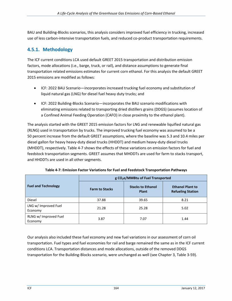
A Life-Cycle Analysis of the Greenhouse Gas Emissions of Corn-Based Ethanol
ICF 164 January 12, 2017
BAU and Building-Blocks scenarios, this analysis considers improved fuel efficiency in trucking, increased
use of less carbon-intensive transportation fuels, and reduced co-product transportation requirements.
4.5.1. Methodology
The ICF current conditions LCA used default GREET 2015 transportation and distribution emission
factors, mode allocations (i.e., barge, truck, or rail), and distance assumptions to generate final
transportation related emissions estimates for current corn ethanol. For this analysis the default GREET
2015 emissions are modified as follows:
ICF: 2022 BAU Scenario—incorporates increased trucking fuel economy and substitution of
liquid natural gas (LNG) for diesel fuel heavy duty trucks; and
ICF: 2022 Building-Blocks Scenario—incorporates the BAU scenario modifications with
eliminating emissions related to transporting dried distillers grains (DDGS) (assumes location of
a Confined Animal Feeding Operation (CAFO) in close proximity to the ethanol plant).
The analysis started with the GREET 2015 emission factors for LNG and renewable liquified natural gas
(RLNG) used in transportation by trucks. The improved trucking fuel economy was assumed to be a
50 percent increase from the default GREET assumptions, where the baseline was 5.3 and 10.4 miles per
diesel gallon for heavy heavy-duty diesel trucks (HHDDT) and medium heavy-duty diesel trucks
(MHDDT), respectively. Table 4-7 shows the effects of these variations on emission factors for fuel and
feedstock transportation segments. GREET assumes that MHDDTs are used for farm to stacks transport,
and HHDDTs are used in all other segments.
Table 4-7: Emission Factor Variations for Fuel and Feedstock Transportation Pathways
Fuel and Technology
g CO2e/MMBtu of Fuel Transported
Farm to Stacks Stacks to Ethanol
Plant Ethanol Plant to
Refueling Station
Diesel 37.88 39.65 8.21
LNG w/ Improved Fuel Economy
21.28 25.28 5.02
RLNG w/ Improved Fuel Economy
3.87 7.07 1.44
Our analysis also included these fuel economy and new fuel variations in our assessment of corn oil
transportation. Fuel types and fuel economies for rail and barge remained the same as in the ICF current
conditions LCA. Transportation distances and mode allocations, outside of the removed DDGS
transportation for the Building-Blocks scenario, were unchanged as well (see Chapter 3, Table 3-59).
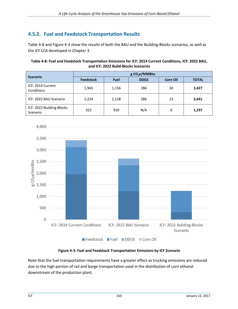
A Life-Cycle Analysis of the Greenhouse Gas Emissions of Corn-Based Ethanol
ICF 165 January 12, 2017
4.5.2. Fuel and Feedstock Transportation Results
Table 4-8 and Figure 4-3 show the results of both the BAU and the Building-Blocks scenarios, as well as
the ICF LCA developed in Chapter 3.
Table 4-8: Fuel and Feedstock Transportation Emissions for ICF: 2014 Current Conditions, ICF: 2022 BAU, and ICF: 2022 Build-Blocks Scenarios
Scenario g CO2e/MMBtu
Feedstock Fuel DDGS Corn Oil TOTAL
ICF: 2014 Current Conditions
1,965 1,156 286 20 3,427
ICF: 2022 BAU Scenario 1,224 1,118 286 13 2,641
ICF: 2022 Building-Blocks Scenario
322 910 N/A 6 1,237
Figure 4-3: Fuel and Feedstock Transportation Emissions by ICF Scenario
Note that the fuel transportation requirements have a greater effect as trucking emissions are reduced
due to the high portion of rail and barge transportation used in the distribution of corn ethanol
downstream of the production plant.
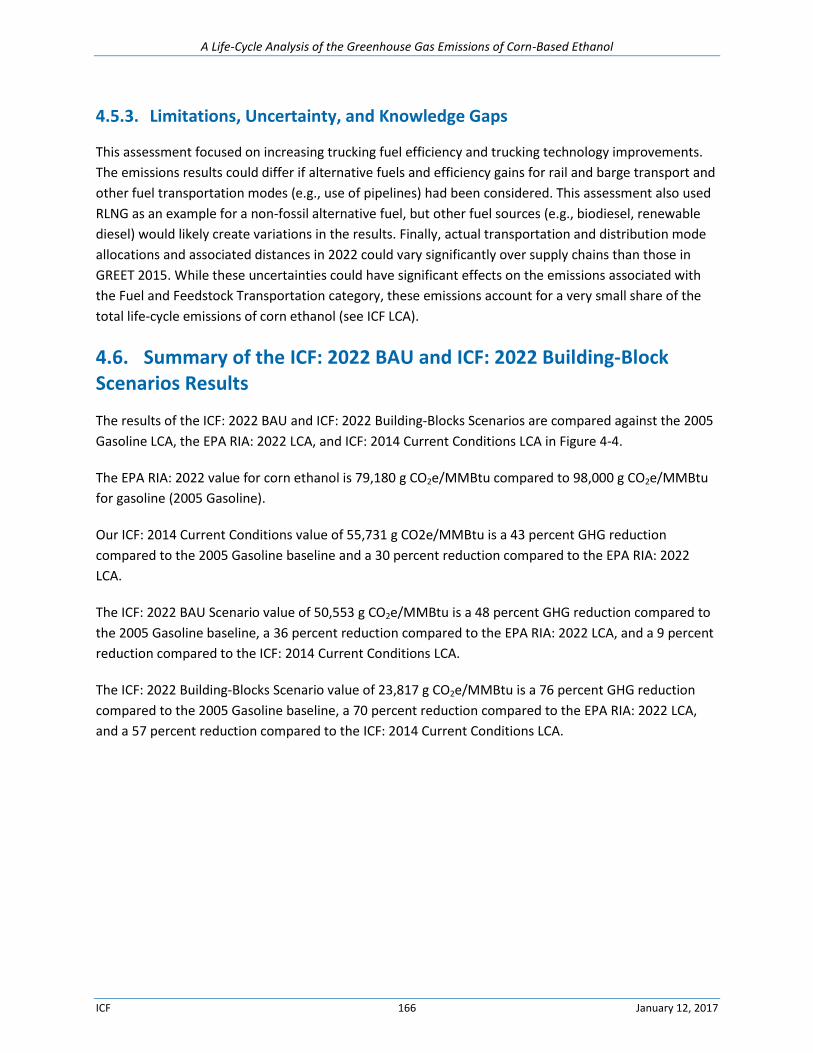
A Life-Cycle Analysis of the Greenhouse Gas Emissions of Corn-Based Ethanol
ICF 166 January 12, 2017
4.5.3. Limitations, Uncertainty, and Knowledge Gaps
This assessment focused on increasing trucking fuel efficiency and trucking technology improvements.
The emissions results could differ if alternative fuels and efficiency gains for rail and barge transport and
other fuel transportation modes (e.g., use of pipelines) had been considered. This assessment also used
RLNG as an example for a non-fossil alternative fuel, but other fuel sources (e.g., biodiesel, renewable
diesel) would likely create variations in the results. Finally, actual transportation and distribution mode
allocations and associated distances in 2022 could vary significantly over supply chains than those in
GREET 2015. While these uncertainties could have significant effects on the emissions associated with
the Fuel and Feedstock Transportation category, these emissions account for a very small share of the
total life-cycle emissions of corn ethanol (see ICF LCA).
4.6. Summary of the ICF: 2022 BAU and ICF: 2022 Building-Block Scenarios Results
The results of the ICF: 2022 BAU and ICF: 2022 Building-Blocks Scenarios are compared against the 2005
Gasoline LCA, the EPA RIA: 2022 LCA, and ICF: 2014 Current Conditions LCA in Figure 4-4.
The EPA RIA: 2022 value for corn ethanol is 79,180 g CO2e/MMBtu compared to 98,000 g CO2e/MMBtu
for gasoline (2005 Gasoline).
Our ICF: 2014 Current Conditions value of 55,731 g CO2e/MMBtu is a 43 percent GHG reduction
compared to the 2005 Gasoline baseline and a 30 percent reduction compared to the EPA RIA: 2022
LCA.
The ICF: 2022 BAU Scenario value of 50,553 g CO2e/MMBtu is a 48 percent GHG reduction compared to
the 2005 Gasoline baseline, a 36 percent reduction compared to the EPA RIA: 2022 LCA, and a 9 percent
reduction compared to the ICF: 2014 Current Conditions LCA.
The ICF: 2022 Building-Blocks Scenario value of 23,817 g CO2e/MMBtu is a 76 percent GHG reduction
compared to the 2005 Gasoline baseline, a 70 percent reduction compared to the EPA RIA: 2022 LCA,
and a 57 percent reduction compared to the ICF: 2014 Current Conditions LCA.
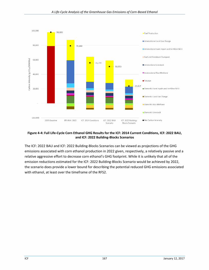
A Life-Cycle Analysis of the Greenhouse Gas Emissions of Corn-Based Ethanol
ICF 167 January 12, 2017
Figure 4-4: Full Life-Cycle Corn Ethanol GHG Results for the ICF: 2014 Current Conditions, ICF: 2022 BAU, and ICF: 2022 Building-Blocks Scenarios
The ICF: 2022 BAU and ICF: 2022 Building-Blocks Scenarios can be viewed as projections of the GHG
emissions associated with corn ethanol production in 2022 given, respectively, a relatively passive and a
relative aggressive effort to decrease corn ethanol’s GHG footprint. While it is unlikely that all of the
emission reductions estimated for the ICF: 2022 Building-Blocks Scenario would be achieved by 2022,
the scenario does provide a lower bound for describing the potential reduced GHG emissions associated
with ethanol, at least over the timeframe of the RFS2.

blankpage