A LiDAR-Aided Indoor Navigation System for UGVs...navigation confronts is the absence of GPS signals in the indoor environment (Misra and Enge, 2001; Noureldin et al., 2012). To handle

A LiDAR-Aided Indoor NavigationSystem for UGVs

Shifei Liu1,3, Mohamed Maher Atia2, Tashfeen B. Karamat3

and Aboelmagd Noureldin2

1 (College of Automation, Harbin Engineering University, China)2 (Department of Electrical & Computer Engineering, Royal Military College

of Canada, Canada)3 (Department of Electrical & Computer Engineering, Queen’s University, Canada)

(E-mail: [email protected])

Autonomous Unmanned Ground Vehicles (UGVs) require a reliable navigation systemthat works in all environments. However, indoor navigation remains a challenge becausethe existing satellite-based navigation systems such as the Global Positioning System (GPS)are mostly unavailable indoors. In this paper, a tightly-coupled integrated navigationsystem that integrates two dimensional (2D) Light Detection and Ranging (LiDAR), InertialNavigation System (INS), and odometry is introduced. An efficient LiDAR-basedline features detection/tracking algorithm is proposed to estimate the relative changes inorientation and displacement of the vehicle. Furthermore, an error model of INS/odometrysystem is derived. LiDAR-estimated orientation/position changes are fused by an ExtendedKalman Filter (EKF) with those predicted by INS/odometry using the developed errormodel. Errors estimated by EKF are used to correct the position and orientation of thevehicle and to compensate for sensor errors. The proposed system is verified throughsimulation and real experiment on an UGV equipped with LiDAR, MEMS-based IMU, andencoder. Both simulation and experimental results showed that sensor errors are accuratelyestimated and the drifts of INS are significantly reduced leading to navigation performanceof sub-metre accuracy.

KEYWORDS

1. LiDAR. 2. Inertial Navigation System. 3. Indoor navigation.4. Unmanned ground vehicle.

Submitted: 3 September 2013. Accepted: 26 July 2014. First published online: 26 September 2014.

1. INTRODUCTION. The promising vista of indoor navigation applicationshave made this area popular with researchers worldwide. One of the challenges indoornavigation confronts is the absence of GPS signals in the indoor environment (Misraand Enge, 2001; Noureldin et al., 2012). To handle this issue, alternative techniquesare introduced to obtain a satisfactory performance. These techniques can be roughlycategorised into two groups depending on the availability of infrastructure and

THE JOURNAL OF NAVIGATION (2015), 68, 253–273. © The Royal Institute of Navigation 2014doi:10.1017/S037346331400054X

https://www.cambridge.org/core/terms. https://doi.org/10.1017/S037346331400054XDownloaded from https://www.cambridge.org/core. IP address: 54.39.106.173, on 31 May 2020 at 08:35:30, subject to the Cambridge Core terms of use, available at

https://www.cambridge.org/core/terms

https://doi.org/10.1017/S037346331400054X

https://www.cambridge.org/core

pre-installed sensor networks. Generally, techniques that are independent of theexternal operational environment are preferred for the consideration of efficiency andcost. To this end, self-contained systems like Inertial Navigation Systems (INS)(Titterton and Weston, 2005) and odometry are widely used in indoor navigation.Particularly, the emergence of the Micro-Electro-Mechanical System (MEMS)-basedINS which is lightweight, and lower in cost and power consumption makes it idealfor personal, mobile robot and aerial vehicle applications (Aggarwal et al., 2010).However, the INS or odometry standalone systems fail to sustain a high accuracy inthe long run due to their inherent error characteristics. This issue can be solved byproviding periodic updates to prevent the error accumulation over time. LightDetection and Ranging (LiDAR) (Harrap and Lato, 2010) and vision (DeSouza andKak, 2002) are two common techniques integrated with INS and odometry in indoornavigation systems. Compared with vision, LiDAR is more accurate and efficient incomputation load and processing speed. Furthermore, LiDAR is not limited bylighting conditions. Therefore, in this paper, we introduce a low-cost lightweightmulti-sensor integrated navigation system that integrates INS/odometry with 2DLiDAR in a tightly coupled scheme to provide a reliable indoor navigation system forUnmanned Ground Vehicles (UGVs). The main contributions introduced in thissystem are summarised as follows:

. INS/odometry is used in a reduced set where only a single vertical gyroscopeis used with the vehicle wheel encoder. This reduces the system complexity andoverall cost.

. An error model of relative displacement/orientation changes is derived for theproposed reduced INS/Odometry system.

. A computationally efficient LiDAR-based line features detection and trackingalgorithm for indoor environments is proposed. The proposed algorithm is moreefficient than traditional curve-fitting-based algorithms.

. A tightly coupled Extended Kalman Filter (EKF) design is proposed for thesystem.

. Both simulation and real experiment with MEMS-grade sensors and a 2D laserscanner from the SICK company are carried out to analyse the performance ofthe proposed work. Extensive analyses of results are given.

. The work introduced in the paper can be used as an in-motion gyroscopecalibration procedure.

. The proposed algorithms can be easily integrated in a more complex multi-sensornavigation system that utilises a variety of other sensors.

2. PREVIOUS WORK. LiDAR has been widely used in ground vehiclesfor the purpose of localisation (Lingemann et al., 2005; Xia et al., 2010), mapping(Barber et al., 2008; Puente et al., 2011) and Simultaneous Localisation and Mapping(SLAM) (Diosi and Kleeman, 2005; Grisetti et al., 2007). However, in most ofthe earlier works using LiDAR alone, they have the drawbacks that LiDAR dependson distinguishable features in the environment and the error in vehicle position derivedby LiDAR will accumulate. Therefore, the integration of LiDAR and INS is essentialto obtain a robust and accurate indoor navigation system. The integration of LiDAR

254 SHIFEI LIU AND OTHERS VOL. 68



https://doi.org/10.1017/S037346331400054X


and INS can be found in both indoor environments and urban areas (Haag et al.,2007), where LiDAR replaces GPS to correct INS periodically. Generally,LiDAR and INS are fused by Extended Kalman Filter (EKF) (Kim et al.,2012; Ma and McKitterick, 2012) or Particle Filter (PF) (Hornung et al., 2010;Bry et al., 2012) in two different schemes. One integration scheme is to feedposition and orientation derived from LiDAR being fed back to the filter tocorrect navigation solutions from INS (Kohlbrecher et al., 2011). This kind ofintegration is called “loosely coupled”. The problem with this kind of integrationis that if the position (and/or) orientation calculated from LiDAR is missing orsignificantly jeopardised, overall accuracy is reduced. In contrast, another methodof integration is defined as “tightly coupled” between LiDAR and INS (Solovievet al., 2007; Soloviev, 2008). In this tightly coupled integration scheme, therelative position and orientation changes estimated by LiDAR are compared withposition and orientation changes predicted by INS/Odometry and the differencesare fed to a filtering module (KF or PF) to estimate both errors in position andorientation changes and sensors biases. This tightly coupled integration scheme iscommonly preferred over loosely coupled integration schemes due to theutilisation of the raw LiDAR measurements and also due to the dependence ofrelative position and orientation changes which are immune to absolute errors inposition and orientation.However, the previous works use full Inertial Measurement Units (IMU) with

complicated mechanisation and error model equations that lead to quicker drifts if notperiodically corrected. In addition, the earlier works commonly utilise a traditionalcurve-fitting-based features detection method that is computationally expensive. Asan improvement to the aforementioned approaches, this paper introduces a reducedsensor set that utilises only a single vertical gyroscope, the vehicle wheel encoder anda 2D LiDAR. An error model is derived and a computationally efficient parallelline features detection and tracking algorithm that efficiently estimates 2D relativeposition and orientation changes is introduced. The reduced sensor set and theefficient line feature extraction and tracking algorithm make the proposed systemsuitable for typical 2D indoor navigation for UGVs.

3. INS/ODOMETRY–BASED NAVIGATION SYSTEM. The pro-posed 2D INS/Odometry-based navigation system consists of one single-axisgyroscope with its sensitive axis aligned with the vertical axis of the body (Iqbalet al., 2009; Iqbal et al., 2010; Atia et al., 2010). The system details are given asfollows.

3.1. System motion model. We assume the vehicle is mostly travelling in thehorizontal plane (Iqbal et al., 2008). Therefore, the forward velocity estimated fromthe vehicle odometry measurements combined with the azimuth obtained fromintegrating gyroscope rotation rate measurements yields velocity, as well asdisplacements, along east and north directions. However, the earth rotation along itsspin axis as well as the change of local level frame (east-north-up) orientation withrespect to the earth will generate a rotation rate component which will also bemeasured by the gyroscope. Thus, these components must be compensated and the

255A LIDAR-AIDED INDOOR NAVIGATION SYSTEM FOR UGVSNO. 2



https://doi.org/10.1017/S037346331400054X


rate of change of azimuth A can be given as follows:

dAdt

= − [wz − bz] − we sin(φ) − ve tan(φ)Rn + h

� �(1)

where φ is latitude, wesin(φ) is earth rotation rate component along thevertical direction, ve is velocity along the east direction, Rn is the earth normalradius of curvature, h is altitude, ve tan(φ)

Rn+h is rotation rate component caused bylocal level frame orientation change and bz is the estimated gyroscope bias usingstationary data.The east and north velocities can be derived from the forward velocity vf

and azimuth A given the assumption that the vehicle is mostly travelling in thehorizontal plane. Velocities along the east and north directions can be writtenrespectively as:

ve = vf sin(A) (2)vn = vf cos(A) (3)

After deriving velocities, 2D position change can be represented as below:

dφdt

= vn

Rm + h(4)

dλdt

= ve

(Rn + h) cos(φ) (5)

whereRm is the earth meridian radius of curvature and λ is longitude. A block diagramdescribing the 2D INS/Odometry system is shown in Figure 1.

3.2. Limitations of INS/Odometry-based navigation system. As self-containedsystems, both INS and odometry can provide navigation independent of their en-vironments. However, the limitations for an INS/Odometry-based navigation systemare obvious. The inertial sensor errors and odometry scale factor error cause drifts thatgrow with time without bound, thus navigation solutions from INS/Odometry-basednavigation systems deteriorate quickly. This gives rise to the requirement of periodiccorrection for the INS/Odometry-based navigation system. In open-sky areas, GPS isthe common correction and aiding source. However, indoors, other aiding sources areneeded.

Figure 1. 2D INS/odometry system.




https://doi.org/10.1017/S037346331400054X


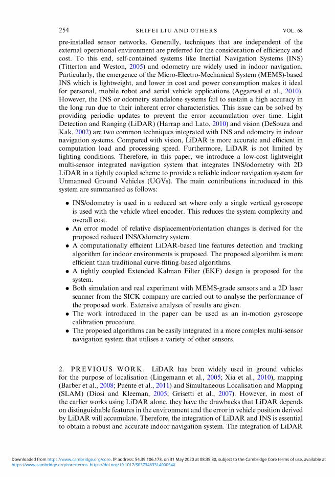
4. THE PROPOSED SYSTEM. The 2D LiDAR (Adams, 2000; Diosi andKleeman, 2003) uses time-of-flight of a laser beam to measure distances from thescanner to the reflecting surrounding objects in a certain angular range with knownangular resolution. Figure 2 shows an example of 2D LiDAR measurements in anindoor corridor where reflections of the two parallel walls are highlighted by solid darklines.In most indoor environments, there exists a common feature that is parallel straight

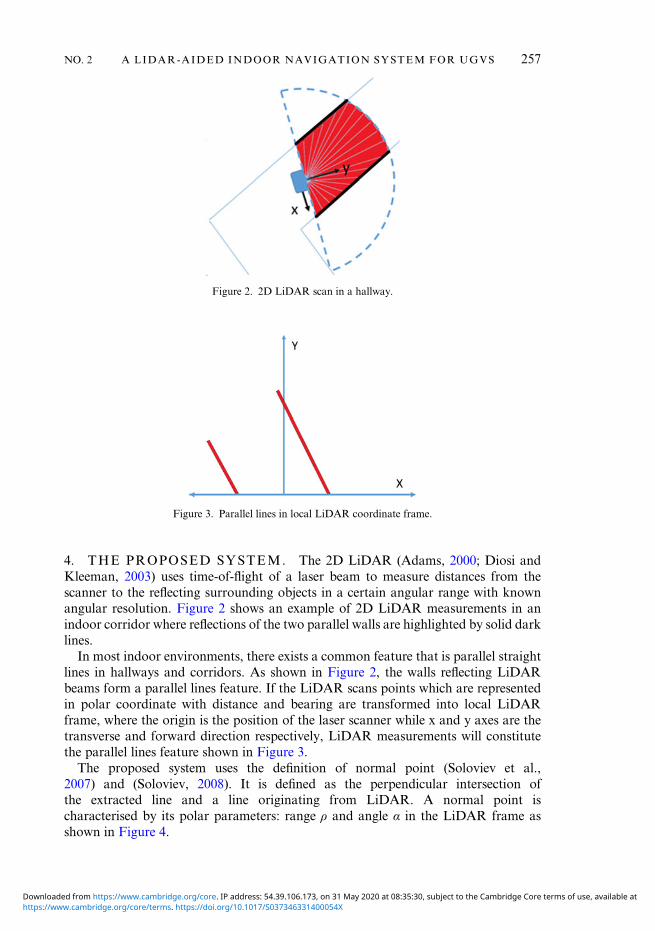
lines in hallways and corridors. As shown in Figure 2, the walls reflecting LiDARbeams form a parallel lines feature. If the LiDAR scans points which are representedin polar coordinate with distance and bearing are transformed into local LiDARframe, where the origin is the position of the laser scanner while x and y axes are thetransverse and forward direction respectively, LiDAR measurements will constitutethe parallel lines feature shown in Figure 3.The proposed system uses the definition of normal point (Soloviev et al.,

2007) and (Soloviev, 2008). It is defined as the perpendicular intersection ofthe extracted line and a line originating from LiDAR. A normal point ischaracterised by its polar parameters: range ρ and angle α in the LiDAR frame asshown in Figure 4.

Figure 2. 2D LiDAR scan in a hallway.

Figure 3. Parallel lines in local LiDAR coordinate frame.




https://doi.org/10.1017/S037346331400054X


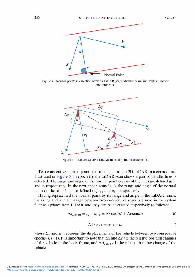
Two consecutive normal point measurements from a 2D LiDAR in a corridor areillustrated in Figure 5. In epoch (i), the LiDAR scan shows a pair of parallel lines isdetected. The range and angle of the normal point on any of the lines are defined as ρiand αi respectively. In the next epoch scan(i+1), the range and angle of the normalpoint on the same line are defined as ρi+1 and αi+1 respectively.Having represented the normal point by its range and angle in the LiDAR frame,

the range and angle changes between two consecutive scans are used in the systemfilter as updates from LiDAR and they can be calculated respectively as follows:

ΔρLiDAR = ρi − ρi+1 = Δx cos(αi) + Δy sin(αi) (6)

ΔALiDAR = αi+1 − αi (7)

where Δx and Δy represent the displacements of the vehicle between two consecutiveepochs (i, i+1). It is important to note that Δx and Δy are the relative position changesof the vehicle in the body frame, and ΔALiDAR is the relative heading change of thevehicle.

Figure 4. Normal point: intersection between LiDAR perpendicular beam and walls in indoorenvironments.

Figure 5. Two consecutive LiDAR normal point measurements.




https://doi.org/10.1017/S037346331400054X


4.1. INS/Odometry-based position/orientation changes prediction. The relativeorientation change and horizontal position change in the vehicle body frame fromepoch (i) to epoch (i+1) can be predicted using INS/Odometry measurements asfollows:

ΔAINS = (wz − bz)T (8)where ΔAINS is the heading change, wz is the gyroscope measurements, bz is thegyroscope bias, and T is the sampling period. By projecting velocity in the body frameat epoch (i), velocity components along xi and yi axis vx and vy can be calculated by:

vx = vf sin(ΔAINS) (9)vy = vf cos(ΔAINS) (10)

where vf is the vehicle odometry measurement. Together with these velocitycomponents, the predicted displacements of the vehicle from epoch (i) to epoch(i+1) ΔxINS and ΔyINS are estimated by:

ΔxINS = vxT (11)ΔyINS = vy T (12)

Substituting Equations (9) to (12) into Equation (6), the range change from INS canbe obtained as follows:

ΔρINS = ΔxINS cos(αi) + ΔyINS sin(αi) (13)4.2. INS/Odometry/LiDAR dynamic error model. In order to use EKF for the

proposed system, a linear dynamic system error model that can be written in thefollowing form has to be obtained:

δx = Fδx+ G w (14)where δx is the error state vector, F is the transition matrix, G is noise parametermatrix and w is the zero mean Gaussian noise vector whose covariance matrix Q isdefined as the system noise matrix given by:

Q =, wwT . (15)In the proposed system, the error state vector is defined as:

δx = [δΔx δΔy δvf δvx δvy δΔA δaod δbz]T

where δΔx is displacement error along x axis of the body frame, δΔy is displacementerror along y axis of the body frame, δvf is odometry measurements error, δvx isvelocity error along x axis, δvy is velocity error along y axis, δΔA is azimuth changeerror, δaod is error in acceleration derived from odometry measurements and δbz iserror in gyroscope bias. By applying a Taylor expansion to the INS/Odometry-baseddynamic system given in Equations (8) to (12) and considering only the first orderterm, the linearized dynamic system error model is given as:

δΔx = δvx (16)δΔy = δvy (17)δvf = δaod (18)




https://doi.org/10.1017/S037346331400054X


δvx = sin(ΔA)δaod + cos(ΔA)(wz − bz)δvf+ aod cos(ΔA) − vf sin(ΔA)(wz − bz)

� �× δΔA− vf cos(ΔA)δbz

(19)

δvy = cos(ΔA)δaod − sin(ΔA)(wz − bz)δvf− aod sin(ΔA) + vf cos(ΔA)(wz − bz)

� �× δΔA+ vf sin(ΔA)δbz

(20)

δΔA = −δbz (21)

δaod = −γodδaod +ffiffiffiffiffiffiffiffiffiffiffiffiffiffiffi2γodσ

2od

qw (22)

δbz = −βzδbz +ffiffiffiffiffiffiffiffiffiffiffiffi2βzσ2z

qw (23)

Here, both random errors in acceleration derived from odometry and gyroscopemeasurements are modelled as first order Gauss-Markov processes. γod and βz arethe reciprocal of the correlation time constants of the random process associatedwith odometry and gyroscope measurements respectively while σod and σz are standarddeviation of this random process (Iqbal et al., 2008).

4.3. INS/Odometry/LiDAR measurement model. The measurement z is modelledas the following form:

z = Hδx+ v (24)Where the observation vector z is defined by:

z = ΔρLiDAR − ΔρINSΔALiDAR − ΔAINS

� �(25)

H is the design matrix of the filter and can be given as:

H = cos(αi) sin(αi) 0 0 0 0 0 00 0 0 0 0 1 0 0

� �(26)

v is the vector of observation random noise, which is assumed to be a zero meanGaussian noise vector whose covariance matrix R is defined as the system noise matrixgiven by:

R =, vvT . (27)From system error model Equations (16) to (23), F and G matrices can be easily

derived. Based on this, the discrete state transition matrix can be given as:

Φk,k+1 = I+ FT (28)where T is the sampling period and I is the identity matrix. Then EKF equations canbe applied to predict the error state vector and update it when measurements fromLiDAR are available. The prediction and correction are performed in the body frameand then transformed into the navigation frame to provide corrected navigationoutput. A block diagram describing the system is shown in Figure 6.




https://doi.org/10.1017/S037346331400054X


5. LINES DETECTION/TRACKING ALGORITHM. Commonly, todetect lines in the environment using LiDAR, a curve-fitting algorithm is used in amoving window that runs over LiDAR scans (Nguyen et al., 2005). Performing thisoperation is a computational bottleneck. To overcome this limitation, we propose amore efficient detection and tracking mechanism that does not need curve fittingand does not involve matrix inversions. Since we target parallel lines in indoorenvironments, we make use of the fact that we have prior knowledge about thetargeted line features. The algorithm consists of two main steps: acquisition andtracking which is similar to the approach used in GPS receivers to acquire satellitesignals (Misra and Enge, 2001). These two steps are described as follows:

. Acquisition Mode: The algorithm performs a search in the space of possiblelateral distances (distance between vehicle position and “Normal Point”)and possible vehicle headings (could be centred on azimuth calculated byINS/Odometry motion model). This search is conducted as follows:○ Based on the lateral distance, heading, and the assumption that a parallel line

feature exists, artificial LiDAR range/angle points are generated. We call thesepoints the “replica”.

○ Whenever a LiDAR measurement is available, the replica is correlated withthe real measurements. If the correlation is strong, the acquisition is declaredto be true and “Normal Points” parameters are calculated.

. Tracking Mode: Once the acquisition mode detects a parallel line feature, thealgorithm will switch to tracking mode. In the tracking mode, the new epoch’sLiDAR measurements are predicted and consequently, the search window isgreatly reduced and the search process becomes quite efficient and more accurate.

. Re-acquisition: In the tracking mode, if the correlation starts to be weak, thetracking mode is halted and the algorithm switches to the acquisition mode.

. INS/Odometry Aiding: To enhance the performance, the INS/Odometryprediction of relative displacement/orientation changes is used to enhance theconsistency and further improve the accuracy and the performance.

Figure 6. INS/Odometry/LiDAR system.




https://doi.org/10.1017/S037346331400054X


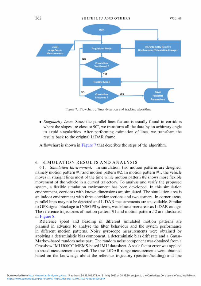
. Singularity Issue: Since the parallel lines feature is usually found in corridorswhere the slopes are close to 90o, we transform all the data by an arbitrary angleto avoid singularities. After performing estimation of lines, we transform theresults back to the original LiDAR frame.

A flowchart is shown in Figure 7 that describes the steps of the algorithm.

6. SIMULATION RESULTS AND ANALYSIS6.1. Simulation Environment. In simulation, two motion patterns are designed,

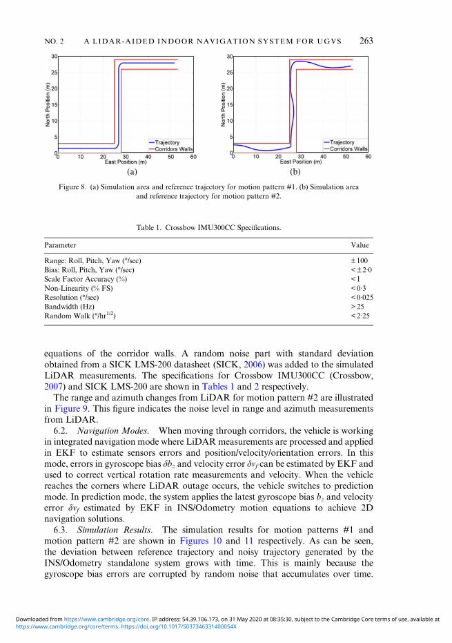
namely motion pattern #1 and motion pattern #2. In motion pattern #1, the vehiclemoves in straight lines most of the time while motion pattern #2 shows more flexiblemovement of the vehicle in a curved trajectory. To analyse and verify the proposedsystem, a flexible simulation environment has been developed. In this simulationenvironment, corridors with known dimensions are simulated. The simulation area isan indoor environment with three corridor sections and two corners. In corner areas,parallel lines may not be detected and LiDAR measurements are unavailable. Similarto GPS signal blockage in INS/GPS systems, we define corner areas as LiDAR outage.The reference trajectories of motion pattern #1 and motion pattern #2 are illustratedin Figure 8.Reference speed and heading in different simulated motion patterns are

planned in advance to analyse the filter behaviour and the system performancein different motion patterns. Noisy gyroscope measurements were obtained byapplying a deterministic bias component, a deterministic bias drift rate and a Gauss-Markov-based random noise part. The random noise component was obtained from aCrossbow IMU300CCMEMS-based IMU datasheet. A scale factor error was appliedto speed measurements as well. The true LiDAR range measurements were obtainedbased on the knowledge about the reference trajectory (position/heading) and line

Figure 7. Flowchart of lines detection and tracking algorithm.




https://doi.org/10.1017/S037346331400054X


equations of the corridor walls. A random noise part with standard deviationobtained from a SICK LMS-200 datasheet (SICK, 2006) was added to the simulatedLiDAR measurements. The specifications for Crossbow IMU300CC (Crossbow,2007) and SICK LMS-200 are shown in Tables 1 and 2 respectively.The range and azimuth changes from LiDAR for motion pattern #2 are illustrated

in Figure 9. This figure indicates the noise level in range and azimuth measurementsfrom LiDAR.

6.2. Navigation Modes. When moving through corridors, the vehicle is workingin integrated navigation mode where LiDARmeasurements are processed and appliedin EKF to estimate sensors errors and position/velocity/orientation errors. In thismode, errors in gyroscope bias δbz and velocity error δvf can be estimated by EKF andused to correct vertical rotation rate measurements and velocity. When the vehiclereaches the corners where LiDAR outage occurs, the vehicle switches to predictionmode. In prediction mode, the system applies the latest gyroscope bias bz and velocityerror δvf estimated by EKF in INS/Odometry motion equations to achieve 2Dnavigation solutions.

6.3. Simulation Results. The simulation results for motion patterns #1 andmotion pattern #2 are shown in Figures 10 and 11 respectively. As can be seen,the deviation between reference trajectory and noisy trajectory generated by theINS/Odometry standalone system grows with time. This is mainly because thegyroscope bias errors are corrupted by random noise that accumulates over time.

(a) (b)

Figure 8. (a) Simulation area and reference trajectory for motion pattern #1. (b) Simulation areaand reference trajectory for motion pattern #2.

Table 1. Crossbow IMU300CC Specifications.

Parameter Value

Range: Roll, Pitch, Yaw (°/sec) ±100Bias: Roll, Pitch, Yaw (°/sec) <±2·0Scale Factor Accuracy (%) <1Non-Linearity (% FS) <0·3Resolution (°/sec) <0·025Bandwidth (Hz) >25Random Walk (°/hr1/2) <2·25




https://doi.org/10.1017/S037346331400054X


However, the LiDAR-aided system can keep close track of the reference movementduring the whole process. During LiDAR outages, the latest estimations of gyroscopebias and odometry velocity error from EKF are accurate enough to maintain a reliableperformance.Owing to measurement updates from LiDAR in EKF, the noises in both gyroscope

and odometry are estimated and compensated, thus leading to long-term sustainable

Table 2. SICK LMS-200 Specifications.

Parameter Value

Statistical Error (mm) 5Angular Resolution (°) 0·5Maximum Measurement Range (m) 80Scanning Range (°) 180

(a) (b)

Figure 9. (a) Noise level of range change from LiDAR measurements. (b) Noise level of azimuthchange from LiDAR measurements.

Figure 10. LiDAR-aided solutions for motion pattern #1.




https://doi.org/10.1017/S037346331400054X


centimetre-level accuracy. The true gyroscope bias and the estimated gyroscope biasfrom EKF in motion pattern #1 and #2 are shown in Figures 12 and 13 respectively.As can be seen from the figures, EKF can accurately estimate the gyroscope bias anddrifts regardless of the motion patterns designed in the simulation experiment. DuringLiDAR outages, the system operates only in prediction mode and gyroscope keepsconstant until LiDAR measurements become available again.The root mean square error in position for motion pattern #1 and #2 in three

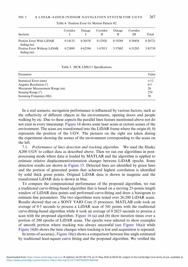
corridor sections and two outages are depicted in Tables 3 and 4 respectively. Fromthese tables, it is worth noting that the performance of motion pattern #2 is betterthan that of motion pattern #1. The reason for this is that in motion pattern #1 thevehicle moves in straight lines most of the time and, consequently, the angle of normal

Figure 11. LiDAR-aided solutions for motion pattern #2.

Figure 12. Gyroscope bias estimation results for motion pattern #1.




https://doi.org/10.1017/S037346331400054X


point at any scan epoch is either 0° or 180°. Substituting this angle value into designmatrix H given in Equation (26) makes the observability of H for the second elementin the error state vector zero. This leads to poor estimation of the error states. Incontrast, when the vehicle moves in a curved trajectory, the angle of the normal pointat any scan epoch keeps changing. The observability of H for the second element inthe error state vector is strong enough to estimate errors. Thus, EKF can achievebetter estimation results for the error states.

7. REAL EXPERIMENT RESULTS AND ANALYSIS. Real experi-ments were conducted in a 70 m by 40m indoor office environment in the RoyalMilitary College of Canada with UGV “Husky A200” from Clearpath Robotics Inc.(Canada-based). The complete loop in the testing trajectory is around 220m and ittook around seven minutes to travel using the Husky A200 UGV. The UGV isequipped with SICK laser scanner LMS111, MEMS level inertial sensor set CHR-UM6 and a quadrature encoder. For the datasheet of CHR-UM6, one can refer toCHRobotics (2013). The specification of SICK LMS111 is shown as below. Thesampling frequency for gyroscope, wheel encoder and laser scanner are 20 Hz, 10 Hzand 50Hz respectively.

Figure 13. Gyroscope bias estimation results for motion pattern #2.

Table 3. Position Error for Motion Pattern #1.

SectionsCorridor Outage Corridor Outage Corridor

TotalI I II II III

Postion Error With LiDARAiding (m)

0·40929 0·50381 0·45845 0·30675 0·61706 0·49438

Postion Error Without LiDARAiding (m)

0·16039 0·51875 1·89935 3·90525 6·64491 3·86072




https://doi.org/10.1017/S037346331400054X


In a real scenario, navigation performance is influenced by various factors, such asthe reflectivity of different objects in the environments, opening doors and peoplewalking by etc. Due to these aspects the parallel lines feature mentioned above not donot exist in every timestamp. Figure 14 shows some laser scans at certain scenes of theenvironment. The scans are transformed into the LiDAR frame where the origin (0, 0)represents the position of the UGV. The pictures on the right are taken duringthe experiment showing the scenes of the environment corresponding to the scans onthe left.

7.1. Performance of lines detection and tracking algorithm. We used the HuskyA200 UGV to collect data as described above. Then we ran our algorithms in post-processing mode where data is loaded by MATLAB and the algorithm is applied toestimate relative displacement/orientation changes between LiDAR epochs. Somedetection results are shown in Figure 15. Detected lines are identified by green linesand the portion of generated points that achieved highest correlation is identifiedby solid thick green points. Original LiDAR data is shown in magenta and thetransformed LiDAR data is shown in blue.To compare the computational performance of the proposed algorithm, we run

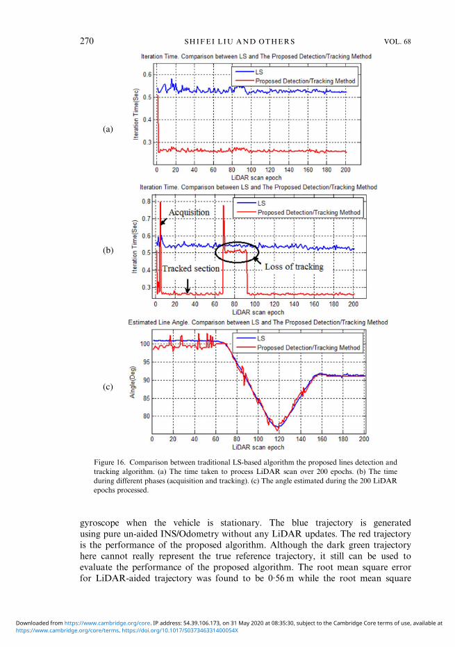
a traditional curve-fitting-based algorithm that is based on a moving 25-points lengthwindow of LiDAR data points and performed curve-fitting and draw a histogram toestimate line parameters. The two algorithms were tested over 26,200 LiDAR scans.Results showed that on a SONY VAIO Core i5 processor, MATLAB code took anaverage of 0·5 seconds to process a LiDAR scan of 541 points with the traditionalcurve-fitting-based algorithm while it took an average of 0·2623 seconds to process ascan with the proposed algorithm. Figure 16 (a) and (b) show iteration times over aportion of 200 epochs of LiDAR scans. The epochs were selected to show examplesof smooth portion where tracking was always successful (see Figure 16(a)) whileFigure 16(b) shows the time changes when tracking is lost and acquisition is repeated.In terms of accuracy, Figure 16(c) shows a comparison between line angle estimated

by traditional least-square curve fitting and the proposed algorithm. We verified the

Table 4. Position Error for Motion Pattern #2.

SectionsCorridor Outage Corridor Outage Corridor

TotalI I II II III

Postion Error With LiDARAiding (m)

0·14133 0·20538 0·12926 0·19289 0·30458 0·20721

Postion Error Without LiDARAiding (m)

0·23889 0·62594 1·67813 3·57002 6·55205 3·85759

Table 5. SICK LMS111 Specifications.

Parameter Value

Statistical Error (mm) ±12Angular Resolution (°) 0·5Maximum Measurement Range (m) 20Scaning Range (°) 270Scanning Frequency (Hz) 50




https://doi.org/10.1017/S037346331400054X


-

0

5

10

15

20

Y(m

)

-5

0

5

10

15

20

Y(m

)

-3-2

0

2

4

6

8

10

12

Y(m

)

0

5

10

15

Y(m

)

(

(

(4.

-6 -4 -2

0

5

0

5

0

-6 -45

0

5

0

5

0

-2

0

(1.1)

(2.1)

(3.1)

.1)

0 2X(m)

-2X(m)

-1 0X(m)

5 1X(m)

4 6 8

0 2

1 2

0 15

(1.2)

(2.2)

(3.2)

(4.2)

Figure 14. Laser scans and pictures in different scenes of the environment: (1·1) The red circlesshow two opening doors. (2·1) In a corner. (3·1) The red square demonstrates the garbage bins.(4·1) The red square indicates a small part of the wall made of glass that the beams can get through.




https://doi.org/10.1017/S037346331400054X


accuracy by applying the estimated relative displacement/orientation changes to theEKF in the integrated navigation system and we found that the positioning accuracy isaround the same. Although the proposed algorithm, in some situations, might be moresensitive to noise (which can be seen in the first portion of Figure 16(c), experimentalresults of the integrated navigation solution showed that the proposed algorithmperforms similarly to curve-fitting-based methods in terms of accuracy but with almost50% faster processing time.

7.2. Positioning performance of the proposed LiDAR-aided integrated navigationsystem. It is important to note that LiDAR updates are propagated to EKF at thefrequency of 5 Hz for two reasons: firstly to guarantee that measurable relativedisplacement/orientation changes have been obtained and secondly to increaseconfidence in these relative displacement/orientation changes measurements byincreasing Signal-to-Noise Ratio (SNR) in LiDAR corrections. During the wholetrajectory, LiDAR updates were available only 20% of the time while during therest of the time, the system operates in INS/Odometry prediction mode. Figure 17illustrates the time epoch when LiDAR updates are available in red markers on thereference trajectory. As can be seen, LiDAR outages occur in places filled withunorganised objects and corners.The results for real experimental data are shown in Figure 18. The dark green

trajectory is used as a reference trajectory derived by manual calibration of the

(a)

(b)

-6 -4 -2 0 2 4 6-2

0

2

4

6Transformed Scan

Laser Scanner X-axis(m)

Lase

r S

cann

er Y

-axi

s(m

)

-6 -4 -2 0 2 4 6-2

0

2

4

6Original Scan


Lase

r S

cann

er Y

-axi

s(m

)

-6 -4 -2 0 2 4 6-2

0

2

4

6Transformed Scan


Lase

r S

cann

er Y

-axi

s(m

)

-6 -4 -2 0 2 4 6-2

0

2

4

6Original Scan


Lase

r S

cann

er Y

-axi

s(m

)

Figure 15. Two detection results snapshots of the proposed lines detection and tracking algorithm.




https://doi.org/10.1017/S037346331400054X


gyroscope when the vehicle is stationary. The blue trajectory is generatedusing pure un-aided INS/Odometry without any LiDAR updates. The red trajectoryis the performance of the proposed algorithm. Although the dark green trajectoryhere cannot really represent the true reference trajectory, it still can be used toevaluate the performance of the proposed algorithm. The root mean square errorfor LiDAR-aided trajectory was found to be 0·56 m while the root mean square

(a)

(b)

(c)

Figure 16. Comparison between traditional LS-based algorithm the proposed lines detection andtracking algorithm. (a) The time taken to process LiDAR scan over 200 epochs. (b) The timeduring different phases (acquisition and tracking). (c) The angle estimated during the 200 LiDARepochs processed.




https://doi.org/10.1017/S037346331400054X


error for INS/Odometry standalone system is 5·25 m which means almost 90% errorreduction is obtained. Given the fact that the real measurements and real environmentare much more complicated than the simulation conditions, this result can beconsidered consistent with the simulation results where a 94% error reductionis obtained. Figure 19 demonstrates the estimation of gyroscope bias error duringa portion of the experiment. Comparing this figure with Figures 12 and 13, thegyroscope bias estimation results from real experiment match the estimation resultsfrom simulations.

-70 -60 -50 -40 -30 -20 -10 0 10-15

-10

-5

0

5

10

15

20

25

East Position(m)

Nor

th P

ositi

on(m

)

Figure 17. LiDAR updates availability during the whole trajectory.

East Position(m)

Nor

th P

ositi

on(m

)

-60 -50 -40 -30 -20 -10 0 10

-20

-15

-10

-5

0

5

10

15

20

25

referenceINS/OdometryEKF-LiDAR

Figure 18. Real experiment results.




https://doi.org/10.1017/S037346331400054X


8. CONCLUSION. In this paper, a 2D INS/Odometry/LiDAR integratednavigation system that is suitable for UGVs in indoor environments was introduced.The INS/Odometry system was used with a reduced inertial sensor set where only avertically aligned gyroscope is used with the vehicle wheel encoders. In addition, a linefeatures detection and tracking algorithm was proposed that is more efficient thantraditional curve-fitting-based algorithms. The LiDAR measurements were used toestimate position and orientation changes which are fused by EKF with a dynamicerror model of the INS/Odometry system. Navigation states were corrected by EKF-estimated errors while gyroscope measurements were compensated by EKF-estimatedbias. Both simulation and real experimental results in an indoor area showed that thesensors errors are accurately estimated by the proposed EKF scheme. Furthermore,the results showed improvement in navigation performance and robustness in realworld application, thus leading to navigation performance of sub-metre accuracy.

REFERENCES

Adams, M.D. (2000). Lidar design, use, and calibration concepts for correct environmental detection. IEEETransactions on Robotics and Automation, 16(6), 753–61.

Aggarwal, P., Syed, Z., Aboelmagd, N. and Naser, E.-S. (2010). MEMS-based Integrated Navigation.Technology and applications Boston; London: Artech House.

Atia, M.M., Georgy, J., Korenberg, M.J. and Noureldin, A. (2010). Real-time implementation of mixtureparticle filter for 3D RISS/GPS integrated navigation solution. Electronics Letters, 46(15), 1083–1084.

Barber, D., Mills, J. and Smith-Voysey, S. (2008). Geometric validation of a ground-based mobile laserscanning system. ISPRS Journal of Photogrammetry and Remote Sensing, 63(1), 128–141.

Bry, A., Bachrach, A. and Roy, N. (2012). State estimation for aggressive flight in GPS-denied environmentsusing onboard sensing. 2012 IEEE International Conference on Robotics and Automation (ICRA), SaintPaul, MN.

CHRobotics. (2013). UM6 ultra-miniature orientation sensor datasheet. CH Robotics LLC.Crossbow. (2007). IMU User’s Manual-Models IMU300CC, IMU400CC,IMU400CD. CrossbowTechnology, Inc.

DeSouza, G. N. and Kak, A.C. (2002). Vision for mobile robot navigation: A survey. IEEE Transactions onPattern Analysis and Machine Intelligence, 24(2), 237–267.

Diosi, A. and Kleeman, L. (2003). Uncertainty of Line Segments Extracted from Static SICK PLS LaserScans. in Proceedings of Australian Conference on Robotics and Automation.

50 100 150 200 250 300 350 400 450-0.024

-0.023

-0.022

-0.021

-0.02

-0.019

-0.018

-0.017

Time(s)

Gyr

osco

pe B

isa

(rad

/s)

Figure 19. Gyroscope bias estimation results for real experiment.




https://doi.org/10.1017/S037346331400054X


Diosi, A. and Kleeman, L. (2005). Laser Scan Matching in Polar Coordinates with Application to SLAM.IEEE/RSJ International Conference on Intelligent Robots and Systems (IROS).

Grisetti, G., Stachniss, C. and Burgard, W. (2007). Improved techniques for grid mapping with Rao-Blackwellized particle filter. IEEE Transactions on Robotics, 23(1), 34–46.

Haag, M.U. d., Venable, D. and Smearcheck, M. (2007). Integration of an inertial measurement unit and3D imaging sensor for urban and indoor navigation of unmanned vehicles Proceedings of the 2007National Technical Meeting of The Institute of Navigation, San Diego, CA.

Harrap, R. and Lato, M. (2010). An overview of LIDAR: collection to application. Norway.Hornung, A., Wurm, K.M. and Bennewitz, M. (2010). Humanoid robot localization in complex indoorenvironments. 2010 IEEE/RSJ International Conference on Intelligent Robots and Systems (IROS).

Iqbal, U., Georgy, J., Korenberg, M. J. and Noureldin, A. (2010). Nonlinear Modeling of Azimuth Errorfor 2D Car Navigation Using Parallel Cascade Identification Augmented with Kalman Filtering.International Journal of Navigation and Observation, 816047 (13 pp.).

Iqbal, U., Karamat, T. B., Okou, A. F. and Noureldin, A. (2009) Experimental Results on an IntegratedGPS and Multisensor System for Land Vehicle Positioning. International Journal of Navigation andObservation, Hindawi Publishing Corporation, 2009.

Iqbal, U., Okou, F. and Noureldin, A. (2008). An Integrated Reduced Inertial Sensor System-RISS/GPSfor Land Vehicles. Proceedings of 2008 IEEE/ION Position, Location and Navigation Symposium,Monterey, CA.

Kim, H.-S., Baeg, S.-H., Yang, K.-W., Cho, K. and Park, S. (2012). An enhanced inertial navigation systembased on a low-cost IMU and laser scanner. Proc. SPIE 8387, Unmanned Systems Technology XIV,83871J.

Kohlbrecher, S., Stryk, O. v., Meyer, J. and Klingauf, U. (2011). A flexible and scalable SLAM system withfull 3D motion estimation. Proceedings of the 2011 IEEE International Symposium on Safety,Security andRescue Robotics, Kyoto, Japan.

Lingemann, K., Nüchter, A., Hertzberg, J. and Surmann, H. (2005). High-speed laser localization formobile robots. Robotics and Autonomous Systems, 51(4), 275–296.

Ma, Y. and McKitterick, J. B. (2012). Range sensor aided inertial navigation using cross correlation on theevidence grid. Proceeding of 2012 IEEE/ION Position Location and Navigation Symposium (PLANS),Myrtle Beach, SC.

Misra, P. and Enge, P. (2001). Global Positioning System : Signals, Measurements, and Performance.Lincoln, Mass.: Ganga-Jamuna Press.

Nguyen, V., Martinelli, A., Tomatis, N. and Siegwart, R. (2005). A comparison of line extractionalgorithms using 2D laser rangefinder for indoor mobile robotics. 2005 IEEE/RSJ InternationalConference on Intelligent Robots and Systems.

Noureldin, A., Karamat, T. B. and Georgy, J. (2012). Fundamentals of Inertial Navigation, Satellite-basedPositioning and their Integration. Heidelberg: Springer.

Puente, I., González-Jorge, H., Arias, P. and Armesto, J. (2011) Land-based mobile laser scanning systems:a review. ISPRS Workshop, Laser Scanning 2011, Calgary, Canada.

SICK. (2006). Technical description: LMS200/211/221/291 laser measurement systems. SICK AG.Soloviev, A. (2008). Tight coupling of GPS, laser scanner, and inertial measurements for navigation inurban environments. 2008 IEEE/ION Symposium on Position, Location and Navigation.

Soloviev, A., Bates, D. and van Graas, F. (2007). Tight coupling of laser scanner and inertial measurementsfor a fully autonomous relative navigation solution. Navigation, 54(3), 189–205.

Titterton, D.H. and Weston, J. (2005). Strapdown Inertial Navigation Technology IEE Radar, Sonar,Navigation and Avionics Series 2nd edn. New York, NY: American Institute of Aeronautics andAstronautics.

Xia, Y., Chun-Xia, Z. and Min, T.Z. (2010). Lidar Scan-Matching for Mobile Robot Localization.Information Technology Journal, 9(1), 27–33.




https://doi.org/10.1017/S037346331400054X


Documents

A LiDAR-Aided Indoor Navigation System for UGVs...navigation confronts is the absence of GPS signals in the indoor environment (Misra and Enge, 2001; Noureldin et al., 2012). To handle