Embed Size (px)
Citation preview
*3368731345*
Further Mathematics A© OCR 2018 [603/1325/0] DC (SC/TP) 159338/3
Oxford Cambridge and RSA
The information in this booklet is for the use of candidates following the Advanced GCE in Further Mathematics A (H245) course.The formulae booklet will be printed for distribution with the examination papers.Copies of this booklet may be used for teaching.This document consists of 16 pages.
Advanced GCE (H245)
Further Mathematics A
Formulae Booklet
Instructions to Exams Officer/Invigilator• Do not send this Formulae Booklet for marking; it should be retained in the centre
or destroyed.
CST322
A Level Further Mathem
atics A
Copyright Information
OCR is committed to seeking permission to reproduce all third-party content that it uses in its assessment materials. OCR has attempted to identify and contact all copyright holders whose work is used in this paper. To avoid the issue of disclosure of answer-related information to candidates, all copyright acknowledgements are reproduced in the OCR Copyright Acknowledgements Booklet. This is produced for each series of examinations and is freely available to download from our public website (www.ocr.org.uk) after the live examination series.
If OCR has unwittingly failed to correctly acknowledge or clear any third-party content in this assessment material, OCR will be happy to correct its mistake at the earliest possible opportunity.
For queries or further information please contact the Copyright Team, First Floor, 9 Hills Road, Cambridge CB2 1GE.
OCR is part of the Cambridge Assessment Group; Cambridge Assessment is the brand name of University of Cambridge Local Examinations Syndicate (UCLES), which is itself a department of the University of Cambridge.
2
Further Mathematics A© OCR 2019
Pure Mathematics
Arithmetic series
( ) ( )S n a l n a n d2 1n 21
21= + = + -" ,
Geometric series
( )S r
a r11
n
n
=--
S ra
1= -3 for r 11
Binomial series
( ) ( ),C C Ca b a a b a b a b b n Nn n n n n n nr
n r r n1
12
2 2 f f !+ = + + + + ++- - -
where ! ( ) !!C C
nr r n r
nnr rn= = =
-
J
LKKN
POO
( ) !( )
!( ) ( )
,x nxn n
x rn n n r
x x n1 1 21 1 1
1 Rn r2 ff
f 1 !+ = + +-
+ +- - +
+ ^ h
Series
( ) ( )r n n n61 1 2 1
r
n2
1= + +
=
/ , ( )r n n41 1
r
n3
1
2 2= +=
/
Maclaurin series
( ) ( ) ( ) !( )
!( )
f f ff f
x x x r x0 00 02
( )rr2 f f= + + + + +l
m
( ) ! !e exp x x xrx1 2
xr2
f f= = + + + + + for all x
( ) ( ) ( )ln l x x x xrx x2 3 1 1 1rr2 3
1f f 1 #+ = - + - + - + -+
! ! ( ) ( ) !sin x x x xrx
3 5 1 2 1r
r3 5 2 1f f= - + - + -
++
+
for all x
! ! ( ) ( ) !cos x x xrx1 2 4 1 2
rr2 4 2
f f= - + - + - + for all x
( ) !( )
!( ) ( )
,x nxn n
x rn n n r
x x n1 1 21 1 1
1 Rn r2 ff
f 1 !+ = + +-
+ +- - +
+ ^ h
Matrix transformations
Reflection in the line :y x01
10!
!
!=
J
LKK
N
POO
Anticlockwise rotation through i about O : cossin
sincos
i
i
i
i
-J
LKK
N
POO
3
Further Mathematics A Turn over© OCR 2019
Rotations through i about the coordinate axes. The direction of positive rotation is taken to be anticlockwise when looking towards the origin from the positive side of the axis of rotation.
cossin
sincos
100
0 0Rx i
i
i
i
= -> H
cos
sin
sin
cos0
010
0Ry
i
i
i
i
=
-> H
cossin
sincos
0 0
001
Rz
i
i
i
i=
-
> H
Differentiation
( )f x ( )f xltan kx seck kx2
sec x sec tanx xcot x cosec x2-
cosec x cosec cotx x-
arcsin x or sin x1- x11
2-
arccos x or cos x1- x11
2-
-
arctan x or tan x1- x112+
Quotient rule , dd d
ddd
y vu
xy
v
v xu u x
v
2= =-
Differentiation from first principles
( )( ) ( )
f limf f
x hx h x
h 0=
+ -
"l
Integration
( )( )
( )ff d ln fxxx x c= +
ly
( ) ( ) ( )f f d fx x x n x c11n n 1
=+
++l ^ ^h hy
Integration by parts dd d d
d du xv x uv v x
u x= -y y

4
Further Mathematics A© OCR 2019
The mean value of ( )f x on the interval [a, b] is ( )f x xb a1 d
a
b
-y
Area of sector enclosed by polar curve is r21 d2 iy
( )f x ( )f x xdy
a x12 2-
sinax x a1 1-J
LKK ^N
POO h
a x1
2 2+tana a
x1 1-J
LKKN
POO
a x12 2+
sinhax1-J
LKKN
POO or ( )ln x x a2 2+ +
x a12 2-
coshax1-J
LKKN
POO or ( ) ( )ln x x a x a2 2 2+ -
Numerical methods
Trapezium rule: {( ) ( ) }dy x h y y y y y2a
bn n2
10 1 2 1f. + + + + +
-y , where h nb a
=-
The Newton-Raphson iteration for solving ( ) : ( )( )
f ff
x x x xx
0 n nn
n1= = -+ l
Complex numbers
Circles: z a k- =
Half lines: ( )arg z a a- =
Lines: z a z b- = -
De Moivre’s theorem: { ( )} ( )cos sin cos sinr r n ni in ni i i i+ = +
Roots of unity: The roots of z 1n = are given by exp iznk2r
=J
LKK
N
POO for , , , ,k n0 1 2 1f= -
Vectors and 3-D coordinate geometry
Cartesian equation of the line through the point A with position vector a i j ka a a1 2 3= + + in direction
u i j ku u u1 2 3= + + is ux a
uy a
uz a
1
1
2
2
3
3 m-
=-
=-
=^ h
Cartesian equation of a plane n x n y n z d 01 2 3+ + + =
Vector product: a baaa
bbb
aaa
bbb
a b a ba b a ba b a b
ijk
1
2
3
1
2
3
1
2
3
1
2
3
2 3 3 2
3 1 1 3
1 2 2 1
# #= = =
-
-
-
J
L
KKKK
J
L
KKKK
J
L
KKKK
N
P
OOOO
N
P
OOOO
N
P
OOOO
5
Further Mathematics A Turn over© OCR 2019
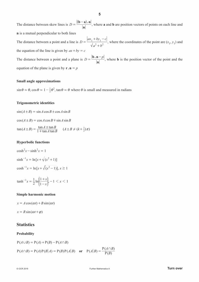
The distance between skew lines is .
Db ann
=-^ h
, where a and b are position vectors of points on each line and
n is a mutual perpendicular to both lines
The distance between a point and a line is Da b
ax by c2 2
1 1=+
+ -, where the coordinates of the point are (x1, y1) and
the equation of the line is given by ax by c+ =
The distance between a point and a plane is .
Dpb n
n=
-, where b is the position vector of the point and the
equation of the plane is given by . pr n =
Small angle approximations
, ,sin cos tan1 21 2. . .i i i i i i- where i is small and measured in radians
Trigonometric identities
( )sin sin cos cos sinA B A B A B! !=
( )cos cos cos sin sinA B A B A B! "=
( ) ( ( ) )tan tan tantan tanA B A BA B A B k1 2
1!"!
! ! r= +
Hyperbolic functions
cosh sinhx x 12 2- =
[ ( )]sinh lnx x x 11 2= + +-
[ ( ],)cosh lnx x x x1 11 2 $= + --
,tanh lnxxx x2
111 1 11 1 1=-
+--
J
LKK
N
POO
Simple harmonic motion
( ) ( )cos sinx A t B t~ ~= +
( )sinx R t~ {= +
Statistics
Probability
( ) ( ) ( ) ( )P P P PA B A B A B, += + -
( ) ( ) ( ) ( ) ( )P P P P PA B A B BA A B+ = = or ( ) ( )( )
P PP
A B BA B+
=

6
Further Mathematics A© OCR 2019
Standard deviation
nx x
nx x
2 22-
= -^ h/ / or f
f x xffx
x2 2
2-= -
^ h/
///
Sampling distributions
For any variable X, ( )XE n= , ( )Var X n2v
= and X is approximately normally distributed when n is large
enough (approximately n 252 )
If ,NX 2+ n v^ h then ,NXn
2+ n
vJ
LKK
N
POO and
/( , )N
nX
0 1+v
n-
Unbiased estimates of the population mean and variance are given by nx/ and n
nnx
nx
12 2
--
J
LKK
J
LKKN
POON
POO
/ /
Expectation algebra
Use the following results, including the cases where a b 1!= = and/or c = 0 :
1. ( ) ( ) ( )aX bY c a X b Y cE E E+ + = + + ,
2. if X and Y are independent then ( ) ( ) ( )Var Var VaraX bY c a X b Y2 2+ + = + .
Discrete distributions
X is a random variable taking values xi in a discrete distribution with P X x pi i= =^ hExpectation: ( )E x pX i in = =/Variance: ( ) ( )Var X x p x pi i i i
2 2 22v n n= = - = -//
( )P X x= ( )E X ( )Var X
Binomial B(n, p)( )
nx p p1x n x- -J
LKKN
POO np ( )np p1-
Uniform distribution over 1, 2, …, n, U(n)n1 n
21+ n12
1 12 -^ h
Geometric distribution Geo(p) ( )p p1 x 1- -
p1
pp12-
Poisson Po(m)!e xxmm- m m
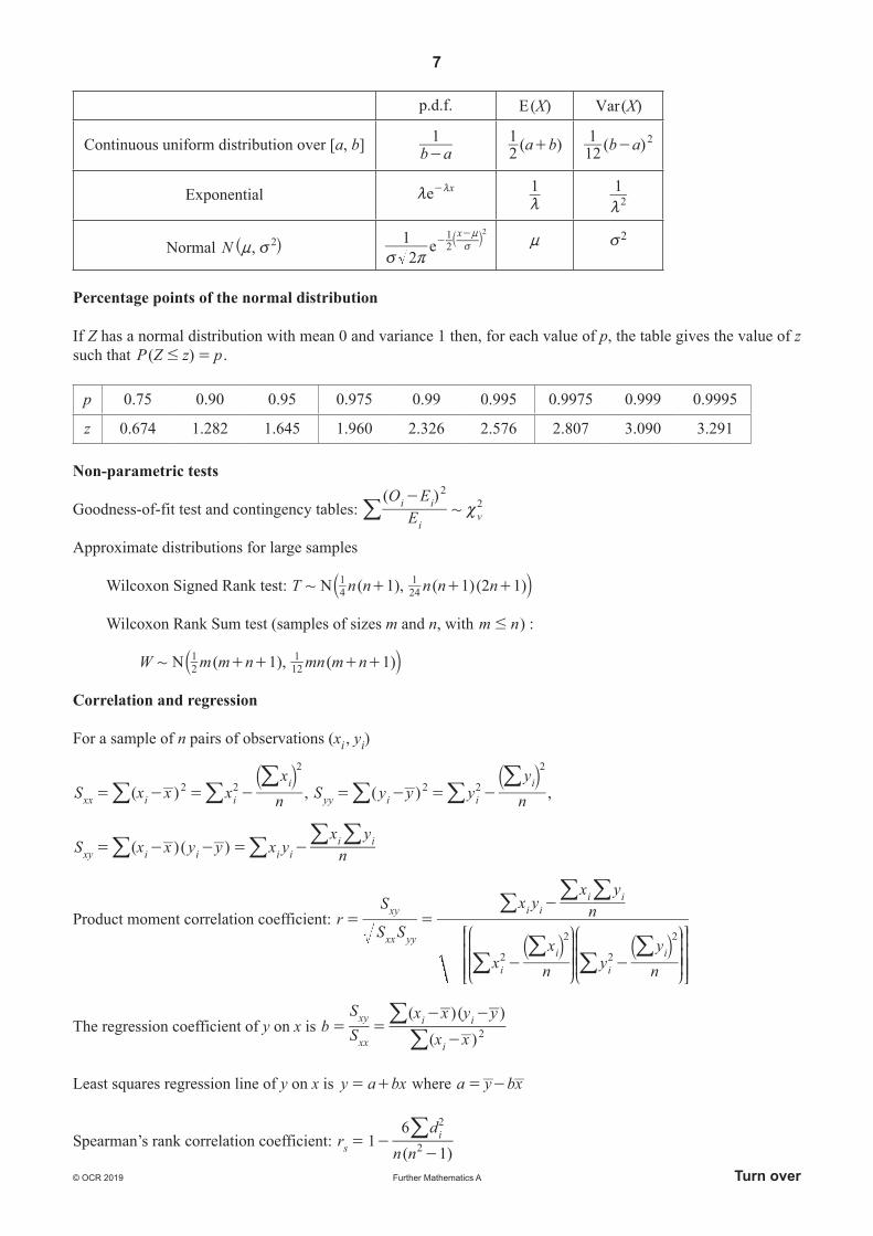
Continuous distributions
X is a continuous random variable with probability density function (p.d.f.) ( )f x
Expectation: ( ) ( )E fX x x xdn = = yVariance: ( ) ( ) ( ) ( )Var f d f dX x x x x x x2 2 2 2v n n= = - = -yyCumulative distribution function ( ) ( ) ( )F P f dx X x t tx
#= =3-y
7
Further Mathematics A Turn over© OCR 2019
p.d.f. ( )E X ( )Var X
Continuous uniform distribution over [a, b] b a1-
( )a b21+ ( )b a12
1 2-
Exponential e xm m- 1m
12m
Normal ,N 2n v^ h21 e
x12
2
v rv
n-
-a k n v2
Percentage points of the normal distribution
If Z has a normal distribution with mean 0 and variance 1 then, for each value of p, the table gives the value of z such that ( )P Z z p# = .
p 0.75 0.90 0.95 0.975 0.99 0.995 0.9975 0.999 0.9995
z 0.674 1.282 1.645 1.960 2.326 2.576 2.807 3.090 3.291
Non-parametric tests
Goodness-of-fit test and contingency tables: ( )OEEi
i
iv
22+ |
-/Approximate distributions for large samples
Wilcoxon Signed Rank test: ( ), ( ) ( )NT n n n n n1 1 2 141
241+ + + +a k
Wilcoxon Rank Sum test (samples of sizes m and n, with m n# ) :
( ), ( )NW m m n mn m n1 121
121+ + + + +a k
Correlation and regression
For a sample of n pairs of observations (xi , yi)
( )S x nx
x xxx ii
i2 2
2
= = --a k
//
/ , ( )S y y y ny
yy i ii2 2
2
= - = -a k
//
/ ,
( ) ( )S x x y y x y nx y
xy i i i ii i= - - = -/ ///
Product moment correlation coefficient: rS S
S
x nx
y ny
x y nx y
xx yy
xy
ii
ii
i ii i
2
2
2
2= =
- -
-
J
L
KKK
J
L
KKK
a aN
P
OOO
N
P
OOO
k kR
T
SSSS
V
X
WWWW
/
//
//
//
The regression coefficient of y on x is (( )) ( )
b SS x x
x xy y
xx
xy i
i
i2= =
-
-
-
//
Least squares regression line of y on x is y a bx= + where a y bx= -
Spearman’s rank correlation coefficient: ( )
rn n
d1
16
si
2
2
= --
/
8
Further Mathem
atics A©
OC
R 2019
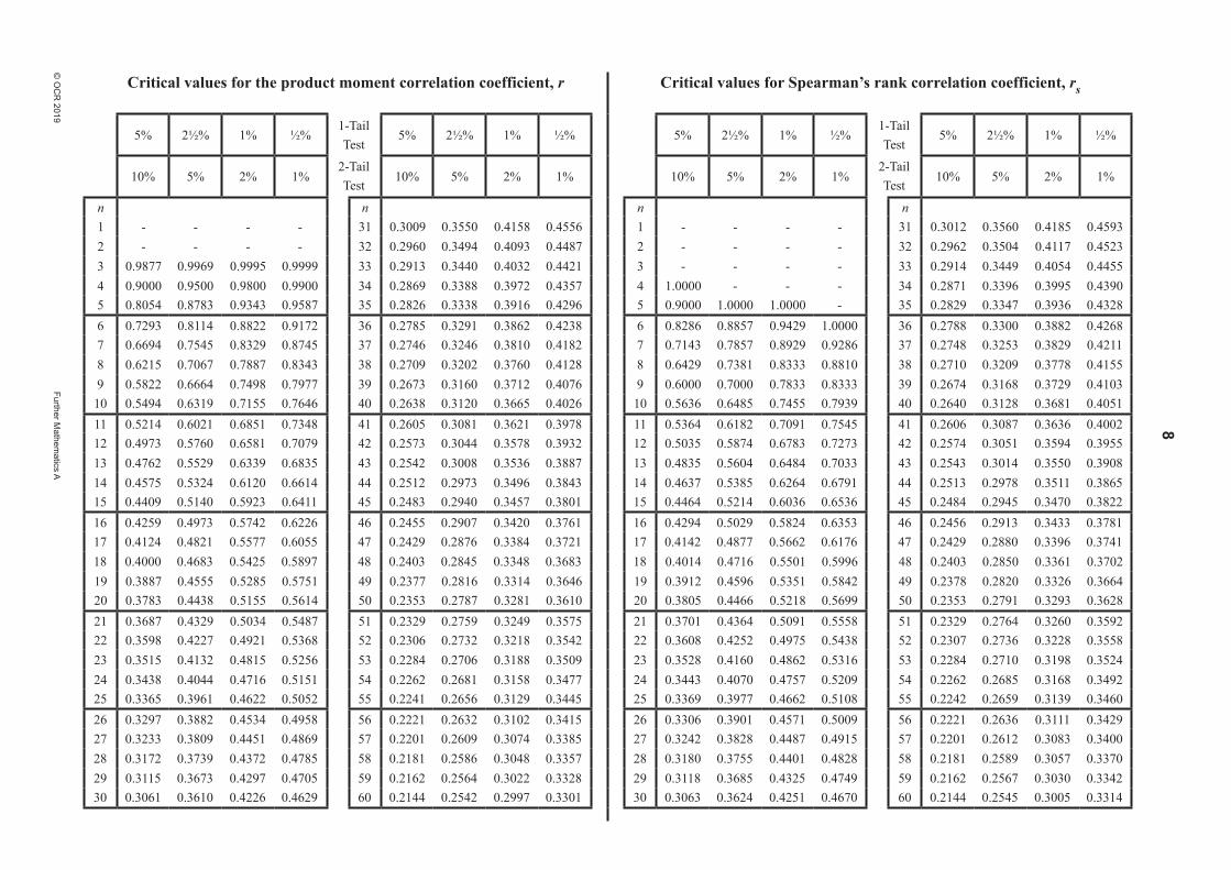
Critical values for the product moment correlation coefficient, r Critical values for Spearman’s rank correlation coefficient, rs
5% 2½% 1% ½%1-Tail Test
5% 2½% 1% ½% 5% 2½% 1% ½%1-Tail Test
5% 2½% 1% ½%
10% 5% 2% 1%2-Tail Test
10% 5% 2% 1% 10% 5% 2% 1%2-Tail Test
10% 5% 2% 1%
n n n n1 - - - - 31 0.3009 0.3550 0.4158 0.4556 1 - - - - 31 0.3012 0.3560 0.4185 0.45932 - - - - 32 0.2960 0.3494 0.4093 0.4487 2 - - - - 32 0.2962 0.3504 0.4117 0.45233 0.9877 0.9969 0.9995 0.9999 33 0.2913 0.3440 0.4032 0.4421 3 - - - - 33 0.2914 0.3449 0.4054 0.44554 0.9000 0.9500 0.9800 0.9900 34 0.2869 0.3388 0.3972 0.4357 4 1.0000 - - - 34 0.2871 0.3396 0.3995 0.43905 0.8054 0.8783 0.9343 0.9587 35 0.2826 0.3338 0.3916 0.4296 5 0.9000 1.0000 1.0000 - 35 0.2829 0.3347 0.3936 0.43286 0.7293 0.8114 0.8822 0.9172 36 0.2785 0.3291 0.3862 0.4238 6 0.8286 0.8857 0.9429 1.0000 36 0.2788 0.3300 0.3882 0.42687 0.6694 0.7545 0.8329 0.8745 37 0.2746 0.3246 0.3810 0.4182 7 0.7143 0.7857 0.8929 0.9286 37 0.2748 0.3253 0.3829 0.42118 0.6215 0.7067 0.7887 0.8343 38 0.2709 0.3202 0.3760 0.4128 8 0.6429 0.7381 0.8333 0.8810 38 0.2710 0.3209 0.3778 0.41559 0.5822 0.6664 0.7498 0.7977 39 0.2673 0.3160 0.3712 0.4076 9 0.6000 0.7000 0.7833 0.8333 39 0.2674 0.3168 0.3729 0.4103
10 0.5494 0.6319 0.7155 0.7646 40 0.2638 0.3120 0.3665 0.4026 10 0.5636 0.6485 0.7455 0.7939 40 0.2640 0.3128 0.3681 0.405111 0.5214 0.6021 0.6851 0.7348 41 0.2605 0.3081 0.3621 0.3978 11 0.5364 0.6182 0.7091 0.7545 41 0.2606 0.3087 0.3636 0.400212 0.4973 0.5760 0.6581 0.7079 42 0.2573 0.3044 0.3578 0.3932 12 0.5035 0.5874 0.6783 0.7273 42 0.2574 0.3051 0.3594 0.395513 0.4762 0.5529 0.6339 0.6835 43 0.2542 0.3008 0.3536 0.3887 13 0.4835 0.5604 0.6484 0.7033 43 0.2543 0.3014 0.3550 0.390814 0.4575 0.5324 0.6120 0.6614 44 0.2512 0.2973 0.3496 0.3843 14 0.4637 0.5385 0.6264 0.6791 44 0.2513 0.2978 0.3511 0.386515 0.4409 0.5140 0.5923 0.6411 45 0.2483 0.2940 0.3457 0.3801 15 0.4464 0.5214 0.6036 0.6536 45 0.2484 0.2945 0.3470 0.382216 0.4259 0.4973 0.5742 0.6226 46 0.2455 0.2907 0.3420 0.3761 16 0.4294 0.5029 0.5824 0.6353 46 0.2456 0.2913 0.3433 0.378117 0.4124 0.4821 0.5577 0.6055 47 0.2429 0.2876 0.3384 0.3721 17 0.4142 0.4877 0.5662 0.6176 47 0.2429 0.2880 0.3396 0.374118 0.4000 0.4683 0.5425 0.5897 48 0.2403 0.2845 0.3348 0.3683 18 0.4014 0.4716 0.5501 0.5996 48 0.2403 0.2850 0.3361 0.370219 0.3887 0.4555 0.5285 0.5751 49 0.2377 0.2816 0.3314 0.3646 19 0.3912 0.4596 0.5351 0.5842 49 0.2378 0.2820 0.3326 0.366420 0.3783 0.4438 0.5155 0.5614 50 0.2353 0.2787 0.3281 0.3610 20 0.3805 0.4466 0.5218 0.5699 50 0.2353 0.2791 0.3293 0.362821 0.3687 0.4329 0.5034 0.5487 51 0.2329 0.2759 0.3249 0.3575 21 0.3701 0.4364 0.5091 0.5558 51 0.2329 0.2764 0.3260 0.359222 0.3598 0.4227 0.4921 0.5368 52 0.2306 0.2732 0.3218 0.3542 22 0.3608 0.4252 0.4975 0.5438 52 0.2307 0.2736 0.3228 0.355823 0.3515 0.4132 0.4815 0.5256 53 0.2284 0.2706 0.3188 0.3509 23 0.3528 0.4160 0.4862 0.5316 53 0.2284 0.2710 0.3198 0.352424 0.3438 0.4044 0.4716 0.5151 54 0.2262 0.2681 0.3158 0.3477 24 0.3443 0.4070 0.4757 0.5209 54 0.2262 0.2685 0.3168 0.349225 0.3365 0.3961 0.4622 0.5052 55 0.2241 0.2656 0.3129 0.3445 25 0.3369 0.3977 0.4662 0.5108 55 0.2242 0.2659 0.3139 0.346026 0.3297 0.3882 0.4534 0.4958 56 0.2221 0.2632 0.3102 0.3415 26 0.3306 0.3901 0.4571 0.5009 56 0.2221 0.2636 0.3111 0.342927 0.3233 0.3809 0.4451 0.4869 57 0.2201 0.2609 0.3074 0.3385 27 0.3242 0.3828 0.4487 0.4915 57 0.2201 0.2612 0.3083 0.340028 0.3172 0.3739 0.4372 0.4785 58 0.2181 0.2586 0.3048 0.3357 28 0.3180 0.3755 0.4401 0.4828 58 0.2181 0.2589 0.3057 0.337029 0.3115 0.3673 0.4297 0.4705 59 0.2162 0.2564 0.3022 0.3328 29 0.3118 0.3685 0.4325 0.4749 59 0.2162 0.2567 0.3030 0.334230 0.3061 0.3610 0.4226 0.4629 60 0.2144 0.2542 0.2997 0.3301 30 0.3063 0.3624 0.4251 0.4670 60 0.2144 0.2545 0.3005 0.3314

9
Further Mathematics A Turn over© OCR 2019
Critical values for the 2| distribution
p
xO
If X has a 2| distribution with v degrees of freedomthen, for each pair of values of p and v, the table givesthe value of x such that ( )P X x p# = .
p 0.01 0.025 0.05 0.90 0.95 0.975 0.99 0.995 0.999v 1= 0.031571 0.039821 0.023932 2.706 3.841 5.024 6.635 7.879 10.83
2 0.02010 0.05064 0.1026 4.605 5.991 7.378 9.210 10.60 13.823 0.1148 0.2158 0.3518 6.251 7.815 9.348 11.34 12.84 16.274 0.2971 0.4844 0.7107 7.779 9.488 11.14 13.28 14.86 18.47
5 0.5543 0.8312 1.145 9.236 11.07 12.83 15.09 16.75 20.516 0.8721 1.237 1.635 10.64 12.59 14.45 16.81 18.55 22.467 1.239 1.690 2.167 12.02 14.07 16.01 18.48 20.28 24.328 1.647 2.180 2.733 13.36 15.51 17.53 20.09 21.95 26.129 2.088 2.700 3.325 14.68 16.92 19.02 21.67 23.59 27.88
10 2.558 3.247 3.940 15.99 18.31 20.48 23.21 25.19 29.5911 3.053 3.816 4.575 17.28 19.68 21.92 24.73 26.76 31.2612 3.571 4.404 5.226 18.55 21.03 23.34 26.22 28.30 32.9113 4.107 5.009 5.892 19.81 22.36 24.74 27.69 29.82 34.5314 4.660 5.629 6.571 21.06 23.68 26.12 29.14 31.32 36.12
15 5.229 6.262 7.261 22.31 25.00 27.49 30.58 32.80 37.7016 5.812 6.908 7.962 23.54 26.30 28.85 32.00 34.27 39.2517 6.408 7.564 8.672 24.77 27.59 30.19 33.41 35.72 40.7918 7.015 8.231 9.390 25.99 28.87 31.53 34.81 37.16 42.3119 7.633 8.907 10.12 27.20 30.14 32.85 36.19 38.58 43.82
20 8.260 9.591 10.85 28.41 31.41 34.17 37.57 40.00 45.3121 8.897 10.28 11.59 29.62 32.67 35.48 38.93 41.40 46.8022 9.542 10.98 12.34 30.81 33.92 36.78 40.29 42.80 48.2723 10.20 11.69 13.09 32.01 35.17 38.08 41.64 44.18 49.7324 10.86 12.40 13.85 33.20 36.42 39.36 42.98 45.56 51.18
25 11.52 13.12 14.61 34.38 37.65 40.65 44.31 46.93 52.6230 14.95 16.79 18.49 40.26 43.77 46.98 50.89 53.67 59.7040 22.16 24.43 26.51 51.81 55.76 59.34 63.69 66.77 73.4050 29.71 32.36 34.76 63.17 67.50 71.42 76.15 79.49 86.6660 37.48 40.48 43.19 74.40 79.08 83.30 88.38 91.95 99.61
70 45.44 48.76 51.74 85.53 90.53 95.02 100.4 104.2 112.380 53.54 57.15 60.39 96.58 101.9 106.6 112.3 116.3 124.890 61.75 65.65 69.13 107.6 113.1 118.1 124.1 128.3 137.2
100 70.06 74.22 77.93 118.5 124.3 129.6 135.8 140.2 149.4

10
Further Mathematics A© OCR 2019
Wilcoxon signed rank test
W+
is the sum of the ranks corresponding to the positive differences,
W-
is the sum of the ranks corresponding to the negative differences,
T is the smaller of W+
and W-
.
For each value of n the table gives the largest value of T which will lead to rejection of the null hypothesis at the level of significance indicated.
Critical values of T
Level of significanceOne Tail 0.05 0.025 0.01 0.005Two Tail 0.10 0.05 0.02 0.01
n = 6 2 0 7 3 2 0 8 5 3 1 0 9 8 5 3 1 10 10 8 5 3 11 13 10 7 5 12 17 13 9 7 13 21 17 12 9 14 25 21 15 12 15 30 25 19 15 16 35 29 23 19 17 41 34 27 23 18 47 40 32 27 19 53 46 37 32 20 60 52 43 37
For larger values of n, each of W+
and W-
can be approximated by the normal distribution with mean ( )n n 141 +
and variance ( ) ( )n n n1 2 1241 + + .
11
Further Mathematics A Turn over© OCR 2019
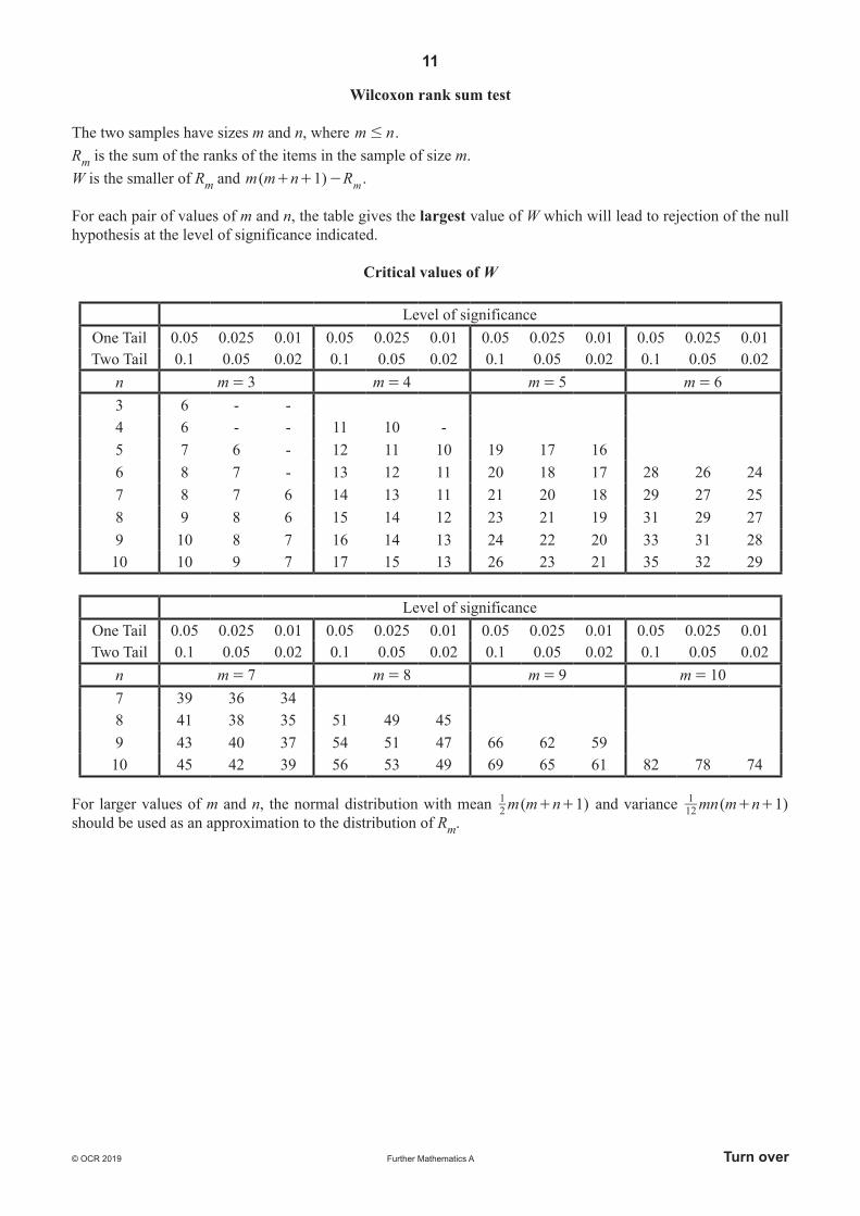
Wilcoxon rank sum test
The two samples have sizes m and n, where m n# .Rm is the sum of the ranks of the items in the sample of size m.W is the smaller of Rm and ( )m m n R1 m+ + - .
For each pair of values of m and n, the table gives the largest value of W which will lead to rejection of the null hypothesis at the level of significance indicated.
Critical values of W
Level of significanceOne Tail 0.05 0.025 0.01 0.05 0.025 0.01 0.05 0.025 0.01 0.05 0.025 0.01Two Tail 0.1 0.05 0.02 0.1 0.05 0.02 0.1 0.05 0.02 0.1 0.05 0.02
n m = 3 m = 4 m = 5 m = 63 6 - -4 6 - - 11 10 -5 7 6 - 12 11 10 19 17 166 8 7 - 13 12 11 20 18 17 28 26 247 8 7 6 14 13 11 21 20 18 29 27 258 9 8 6 15 14 12 23 21 19 31 29 279 10 8 7 16 14 13 24 22 20 33 31 2810 10 9 7 17 15 13 26 23 21 35 32 29
Level of significanceOne Tail 0.05 0.025 0.01 0.05 0.025 0.01 0.05 0.025 0.01 0.05 0.025 0.01Two Tail 0.1 0.05 0.02 0.1 0.05 0.02 0.1 0.05 0.02 0.1 0.05 0.02
n m = 7 m = 8 m = 9 m = 107 39 36 348 41 38 35 51 49 459 43 40 37 54 51 47 66 62 5910 45 42 39 56 53 49 69 65 61 82 78 74
For larger values of m and n, the normal distribution with mean ( )m m n 121 + + and variance ( )mn m n 112
1 + + should be used as an approximation to the distribution of Rm.
12
Further Mathematics A© OCR 2019
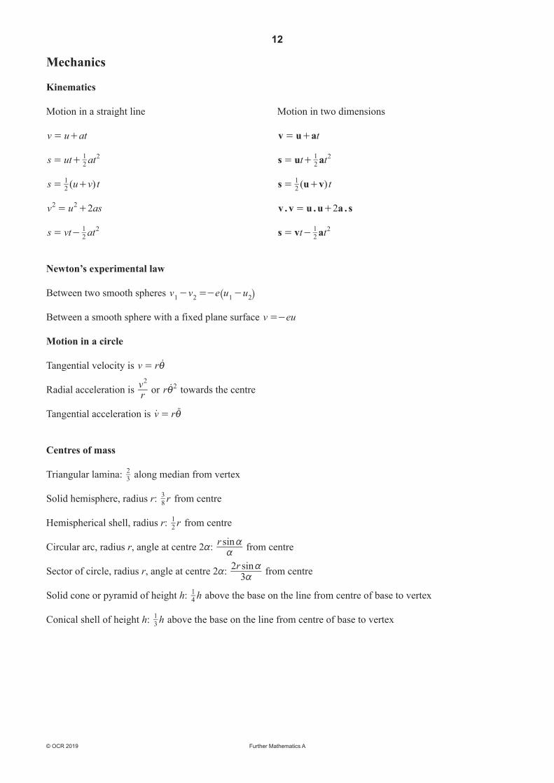
Mechanics
Kinematics
Motion in a straight line Motion in two dimensions
v u at= + tv u a= +
s ut at21 2= + t ts u a2
1 2= +
( )s u v t21= + ( ) ts u v2
1= +
v u as22 2= + . . .2v v u u a s= +
s vt at21 2= - t ts v a2
1 2= -
Newton’s experimental law
Between two smooth spheres v v e u u1 2 1 2- =- -^ hBetween a smooth sphere with a fixed plane surface v eu=-
Motion in a circle
Tangential velocity is v ri= o
Radial acceleration is rv2
or r 2io towards the centre
Tangential acceleration is v ri=o p
Centres of mass
Triangular lamina: 32 along median from vertex
Solid hemisphere, radius r: r83 from centre
Hemispherical shell, radius r: r21 from centre
Circular arc, radius r, angle at centre 2a: sinraa from centre
Sector of circle, radius r, angle at centre 2a: sinr3
2aa from centre
Solid cone or pyramid of height h: h41 above the base on the line from centre of base to vertex
Conical shell of height h: h31 above the base on the line from centre of base to vertex
13
Further Mathematics A Turn over© OCR 2019
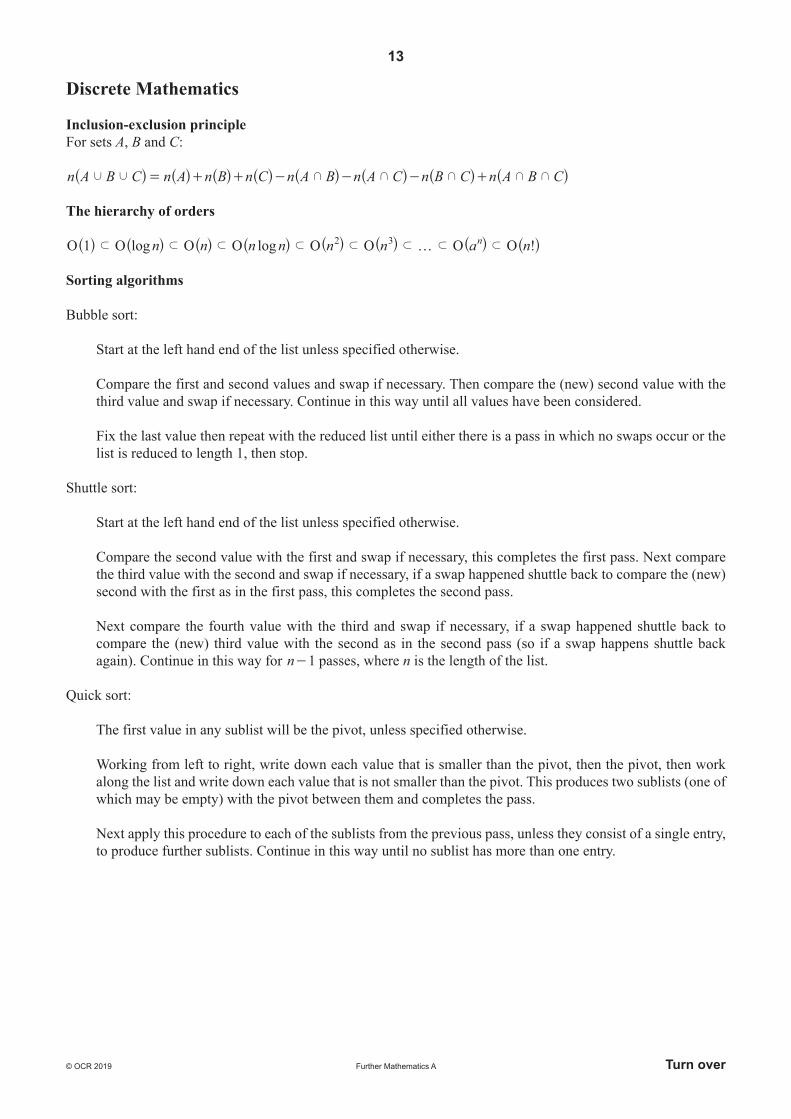
Discrete Mathematics
Inclusion-exclusion principleFor sets A, B and C:
n n n n n n A C n B C n A B CA B C A B C A Bj j k k k k k= + + - - - +^ ^ ^ ^ ^ ^ ^ ^h h h h h h h h
The hierarchy of orders
!O O log O O log O O O On n n n n n a n1 n2 3f f f f f f f ff^ ^ ^ ^ ^ ^ ^ ^h h h h h h h h
Sorting algorithms
Bubble sort:
Start at the left hand end of the list unless specified otherwise.
Compare the first and second values and swap if necessary. Then compare the (new) second value with the third value and swap if necessary. Continue in this way until all values have been considered.
Fix the last value then repeat with the reduced list until either there is a pass in which no swaps occur or the list is reduced to length 1, then stop.
Shuttle sort:
Start at the left hand end of the list unless specified otherwise.
Compare the second value with the first and swap if necessary, this completes the first pass. Next compare the third value with the second and swap if necessary, if a swap happened shuttle back to compare the (new) second with the first as in the first pass, this completes the second pass.
Next compare the fourth value with the third and swap if necessary, if a swap happened shuttle back to compare the (new) third value with the second as in the second pass (so if a swap happens shuttle back again). Continue in this way for n 1- passes, where n is the length of the list.
Quick sort:
The first value in any sublist will be the pivot, unless specified otherwise.
Working from left to right, write down each value that is smaller than the pivot, then the pivot, then work along the list and write down each value that is not smaller than the pivot. This produces two sublists (one of which may be empty) with the pivot between them and completes the pass.
Next apply this procedure to each of the sublists from the previous pass, unless they consist of a single entry, to produce further sublists. Continue in this way until no sublist has more than one entry.
14
Further Mathematics A© OCR 2019
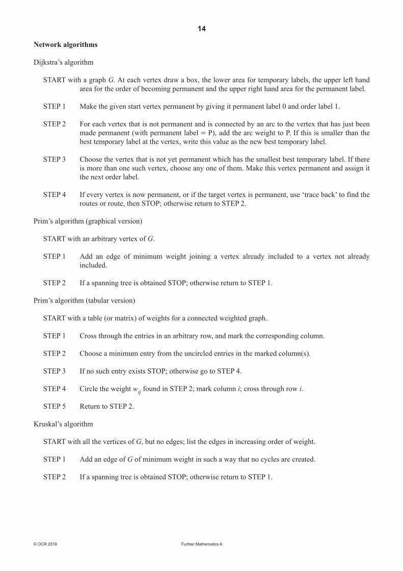
Network algorithms
Dijkstra’s algorithm
START with a graph G. At each vertex draw a box, the lower area for temporary labels, the upper left hand area for the order of becoming permanent and the upper right hand area for the permanent label.
STEP 1 Make the given start vertex permanent by giving it permanent label 0 and order label 1.
STEP 2 For each vertex that is not permanent and is connected by an arc to the vertex that has just been made permanent (with permanent label = P), add the arc weight to P. If this is smaller than the best temporary label at the vertex, write this value as the new best temporary label.
STEP 3 Choose the vertex that is not yet permanent which has the smallest best temporary label. If there is more than one such vertex, choose any one of them. Make this vertex permanent and assign it the next order label.
STEP 4 If every vertex is now permanent, or if the target vertex is permanent, use ‘trace back’ to find the routes or route, then STOP; otherwise return to STEP 2.
Prim’s algorithm (graphical version)
START with an arbitrary vertex of G.
STEP 1 Add an edge of minimum weight joining a vertex already included to a vertex not already included.
STEP 2 If a spanning tree is obtained STOP; otherwise return to STEP 1.
Prim’s algorithm (tabular version)
START with a table (or matrix) of weights for a connected weighted graph.
STEP 1 Cross through the entries in an arbitrary row, and mark the corresponding column.
STEP 2 Choose a minimum entry from the uncircled entries in the marked column(s).
STEP 3 If no such entry exists STOP; otherwise go to STEP 4.
STEP 4 Circle the weight wij found in STEP 2; mark column i; cross through row i.
STEP 5 Return to STEP 2.
Kruskal’s algorithm
START with all the vertices of G, but no edges; list the edges in increasing order of weight.
STEP 1 Add an edge of G of minimum weight in such a way that no cycles are created.
STEP 2 If a spanning tree is obtained STOP; otherwise return to STEP 1.
15
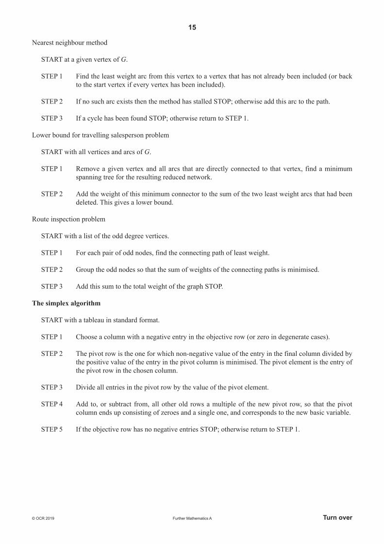
Further Mathematics A Turn over© OCR 2019
Nearest neighbour method
START at a given vertex of G.
STEP 1 Find the least weight arc from this vertex to a vertex that has not already been included (or back to the start vertex if every vertex has been included).
STEP 2 If no such arc exists then the method has stalled STOP; otherwise add this arc to the path.
STEP 3 If a cycle has been found STOP; otherwise return to STEP 1.
Lower bound for travelling salesperson problem
START with all vertices and arcs of G.
STEP 1 Remove a given vertex and all arcs that are directly connected to that vertex, find a minimum spanning tree for the resulting reduced network.
STEP 2 Add the weight of this minimum connector to the sum of the two least weight arcs that had been deleted. This gives a lower bound.
Route inspection problem
START with a list of the odd degree vertices.
STEP 1 For each pair of odd nodes, find the connecting path of least weight.
STEP 2 Group the odd nodes so that the sum of weights of the connecting paths is minimised.
STEP 3 Add this sum to the total weight of the graph STOP.
The simplex algorithm
START with a tableau in standard format.
STEP 1 Choose a column with a negative entry in the objective row (or zero in degenerate cases).
STEP 2 The pivot row is the one for which non-negative value of the entry in the final column divided by the positive value of the entry in the pivot column is minimised. The pivot element is the entry of the pivot row in the chosen column.
STEP 3 Divide all entries in the pivot row by the value of the pivot element.
STEP 4 Add to, or subtract from, all other old rows a multiple of the new pivot row, so that the pivot column ends up consisting of zeroes and a single one, and corresponds to the new basic variable.
STEP 5 If the objective row has no negative entries STOP; otherwise return to STEP 1.
16
Further Mathematics A© OCR 2019
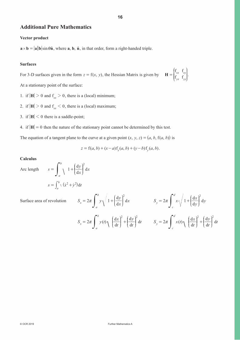
Additional Pure Mathematics
Vector product
sina b a b n# i= t , where a, b, nt , in that order, form a right-handed triple.
Surfaces
For 3-D surfaces given in the form ( , )fz x y= , the Hessian Matrix is given by Hff
ff
xx
yx
xy
yy=
J
L
KKK
N
P
OOO.
At a stationary point of the surface:
1. if H 02 and f 0xx 2 , there is a (local) minimum;
2. if H 02 and f 0xx 1 , there is a (local) maximum;
3. if H 01 there is a saddle-point;
4. if H 0= then the nature of the stationary point cannot be determined by this test.
The equation of a tangent plane to the curve at a given point ( , , ) , , ( , )fx y z a b a b= ^ h is
( , ) ( ) ( , ) ( ) ( , )f f fz a b x a a b y b a bx y= + - + - .
Calculus
Arc length d
dd
sx
xy
1a
b 2
= +J
LKKN
POOy
ds x y ta
b 2 2= +o o^ hy
Surface area of revolution dd
dS yxy
x2 1xa
b 2
r= +J
LKKN
POOy
dd dS xyx y2 1y
c
d 2
r= +J
LKKN
POOy
( )dd
dd
dS y ttx
ty
t2xa
b 2 2
r= +J
LKK
J
LKK
N
POO
N
POOy ( )
dd
dd
dS x ttx
ty
t2yc
d 2 2
r= +J
LKK
J
LKK
N
POO
N
POOy