Embed Size (px)
Citation preview
Progress in Nuclear Enenergy, Vol. 19, No. 2, pp. 137-172, 1987. 0149-1970/87 50.00+ .50 Printed in Great Britain. 1987 Pergamon Journals Ltd.
A LEAST SQUARES PRINCIPLE UNIFYING FINITE ELEMENT, FINITE DIFFERENCE AND NODAL METHODS FOR DIFFUSION THEORY
R. T. ACKROYD
Nuclear Engineering Department, Queen Mary College, University of London, Mile End Road, London El 4NS
(Received 4 June 1986)
Abstract--A least squares principle is described which uses a penalty function treatment of boundary and interface conditions. Appropriate choices of the trial functions and vectors employed in a dual representation of an approximate solution established complementary principles for the diffusion equation. A geometrical interpretation of the principles provides weighted residual methods for diffusion theory, thus establishing a unification of least squares, variational and weighted residual methods.
The complementary principles are used with either a trial function for the flux or a trial vector for the current to establish for regular meshes a connection between finite element, finite difference and nodal methods, which can be exact if the mesh pitches are chosen appropriately. Whereas the coefficients in the usual nodal equations have to be determined iteratively, those derived via the complementary principles are given explicitly in terms of the data.
For the further development of the connection between finite element, finite difference and nodal methods, some hybrid variational methods are described which employ both a trial function and a trial vector.
1. INTRODUCTION
1.1. Scope of the least squares method
A generalized least squares method has been used by Ackroyd (1981), (1982) and (1983) to derive both complementary variational principles and weighted residual methods for the numerical solution of the Boltzmann equation. The same method, shorn of the complexities inherent in its application to the Boltz- mann equation, is developed for the diffusion equation with the aim of providing a unified treatment of finite element, finite difference and nodal methods.
1.1.1. Non-classical variational and weighted residual methods. The least square method leads to a maximum principle which uses a trial function for the flux and a trial vector for the net current. No boundary condi- tions need be imposed on either the trial function or the trial vector. This principle, and its transport theory analogue, provides a means of changing the specifica- tion of the trial function and the trial vector, region by region, according to the physics of the problem. Simple numerical examples of this technique for the Boltz- mann equation are quoted from the work of Ackroyd and Wilson (1985), and Wilson (1985). In the transport theory application the order of the spherical harmonic expansion used to represent the directional is varied from region to region to avoid the burden of a high order spherical harmonic expansion throughout the
system. For diffusion theory the emphasis is placed on a unified treatment of finite element, finite difference and nodal methods. All these methods are obtained from the maximum principle, but they can be obtained using suitable weighted residual procedures. A geo- metrical interpretation of the maximum principle provides an appropriate weighted residual procedure.
1.1.2. Complementary principles of classical kinds. Appropriate choices of trial function and trial vector gives rise to variational principles of classical kinds, i.e. principles for which either the trial function or the trial vector have to satisfy essential boundary conditions. Corresponding to a maximum principle for the flux, there is a complementary minimum principle for the net current. The essential and natural boundary conditions for the maximum principle become the natural and essential boundary conditions respectively for the minimum principle.
I. 1.3. Complementary principles and finite difference methods. Four applications of the principles are given. Firstly the principles are used with finite element representations for the trial function and the trial vector to obtain finite difference equations. For one dimension these finite difference equations closely resemble the classical difference equations. In two dimensions the maximum principle for the flux gives a nine-point scheme in place of the customary five-point
137
138 R.T. ACKROYD
mesh centred scheme. On neglecting fourth order terms in the mesh pitch a five-point scheme of a mesh- centred kind is obtained from the nine-point scheme. For two dimensions the minimum principle for the net current gives rise to two sets of difference equations, for which an explanation is given. At first sight there is only a weak link between this ten-point dual difference scheme with established schemes.
1.1.4. Finite element method analogous to the "nodal' method. The trial vector of the minimum principle is made the gradient of a scalar for each element of the finite element method. If a conservation condition is imposed on an element the components of the trial vector are related to the average flux for the element. Then it is possible to recast the dual ten-point difference scheme as a nine-point scheme in average fluxes. For one dimensional systems the nine-point scheme reduces to a three-point scheme. For two dimensions, when the mesh pitches are related in a certain way to the diffusion length, the nine-point scheme reduces exactly to a five-point scheme. For arbitrary mesh pitches a simple approximation reduces the nine-point scheme to the five-point scheme. Thus there is a close correspondence between the finite element five-point scheme for average fluxes and the usual five-point scheme of the 'nodal' method for the average fluxes. The 'node' of the latter method being the element of the former. Whereas the coeffi- cients in the 'nodal' schemes of Putney (1984) have to be determined iteratively, those for the finite element scheme are given directly in terms of the nuclear data.
1.1.5. Global and local errors. Having obtained a solution to a diffusion problem by some means or other, it is necessary to check the means by reference to some bench mark. Complementary principles can be used to establish measures of overall or global accuracy, and also of local accuracy. Where analytical results for bench marks are not available, complemen- tary principles can establish both global and local measures of accuracy. Ackroyd and Splawski (1982) have shown by example how this can be done for the Boltzmann equation.
As an example of a bench mark for global accuracy the complementary principles for the flux and the net current are used to re-establish bounds, due to Dresner (1961) and Arthurs (1965), for the absorption probabi- lity of a bare sphere.
1.1.6. Complementary hybrid principles. A measure of local accuracy could be obtained with the bi- variational method of Ackroyd and Splawski using the complementary principles for the flux and the net current. Instead another pair of suitable complemen-
tary principles are described. These hybrid principles employ both a trial vector and a trial function in each principle. The maximum principle uses a continuous trial function with no continuity restriction on the trial vector. The opposite holds for the minimum principle, which is a generalization of a classical principle using a continuous trial function. In practice the classical principle is restricted to one dimensional systems because the trial function has to satisfy also a continuity condition on its normal derivative at interfaces. The minimum principle is applied to set up a two dimensional difference scheme for the diffusion equation.
1.2. Representation of approximate solutions
The least squares method for deriving a variety of variational principles and weighted residual methods for the first and second order forms of the Boltzmann equation has been described by Ackroyd (1981), (1982); and Ackroyd (1983). The starting point is the parity equations for ~b~ (r, ~ ) and ~b o (r, ~ ) the even and odd parity components respectively of qSo(r, f~) the angular flux at r for the direction ft. The parity equations
n . V ~ o ~ + G - ' ~ o = S -
n . V,~o + C ~ o = s + (1)
can be regarded as the fundamental equations for neutron transport, because adding the equations gives the first order, or physical, Boltzmann equation and elimination of one of the parity components gives the second order equations for q~- and 4)o. A motivation for resolving 4,0 into its parity components is that ~nq~(r, ~) df~ is the flux at r, and 2 d A S n . n > o ~ - n q ~ o ( r . l l ) d ~ is the net number of neutrons per unit time crossing dA in the same sense as n the normal to dA.
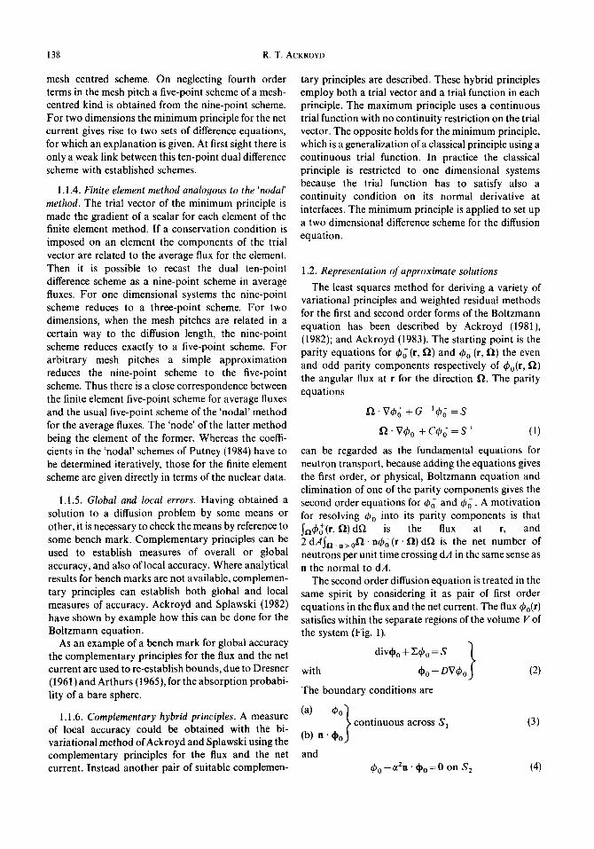
The second order diffusion equation is treated in the same spirit by considering it as pair of first order equations in the flux and the net current. The flux ~bo(r) satisfies within the separate regions of the volume V of the system (Fig. 1).
divd~o + E4~o = S /
with dOo-DV~bo } (2)
The boundary conditions are
(a) 4~o~- continuous across $1 (3)
(b) n . 0 o j
and q9 o - ~2n. d~o = 0 on S 2 (4)
A least squares principle 139
n
a bore surfoce
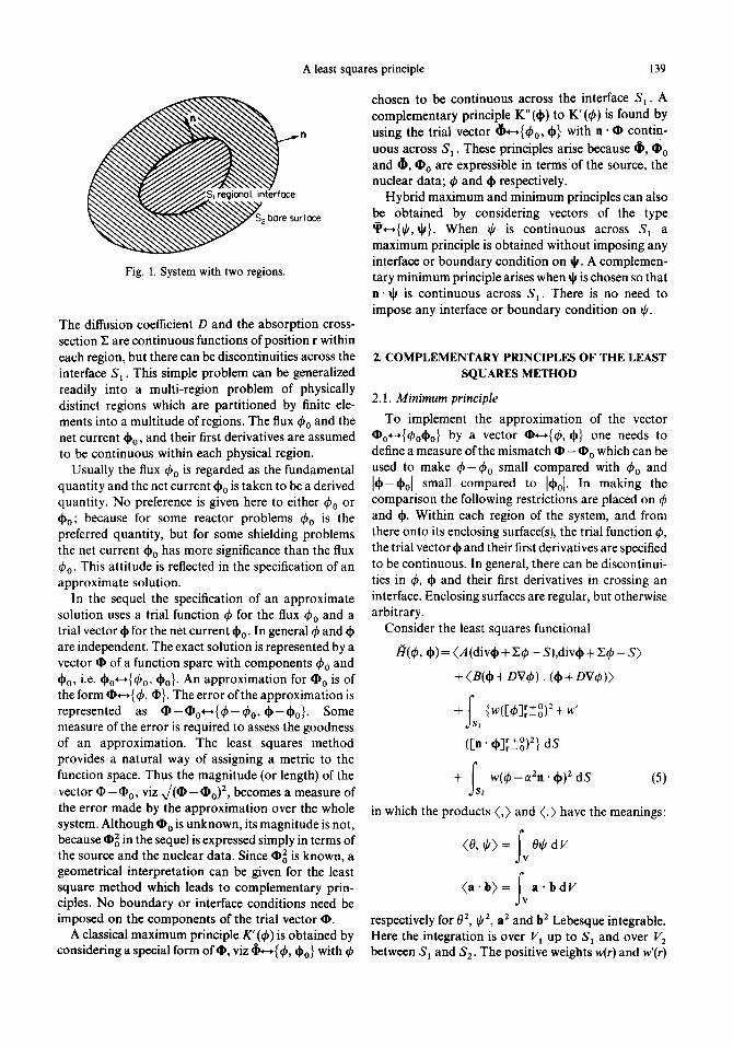
Fig. 1. System with two regions.
The diffusion coefficient D and the absorption cross- section Z are continuous functions of position r within each region, but there can be discontinuities across the interface Sa. This simple problem can be generalized readily into a multi-region problem of physically distinct regions which are partitioned by finite ele- ments into a multitude of regions. The flux ~b 0 and the net current do0, and their first derivatives are assumed to be continuous within each physical region.
Usually the flux ¢0 is regarded as the fundamental quantity and the net current do0 is taken to be a derived quantity. No preference is given here to either q~o or do0; because for some reactor problems ~b 0 is the preferred quantity, but for some shielding problems the net current do0 has more significance than the flux ~b o. This attitude is reflected in the specification of an approximate solution.
In the sequel the specification of an approximate solution uses a trial function ¢ for the flux ¢0 and a trial vector do for the net current do0. In general ~b and do are independent. The exact solution is represented by a vector ~ of a function spare with components ¢0 and do0, i.e. do0~{¢o, do0}- An approximation for ~0 is of the form ~--@k, (I)}. The error of the approximation is represented as ~ -~o~- - ,{¢-q~o , do-do0}. Some measure of the error is required to assess the goodness of an approximation. The least squares method provides a natural way of assigning a metric to the function space. Thus the magnitude (or length) of the vector ~ - ~ 0 , viz x / ( O - ~ o ) 2, becomes a measure of the error made by the approximation over the whole system. Although • 0 is unknown, its magnitude is not, because ~g in the sequel is expressed simply in terms of the source and the nuclear data. Since ~02 is known, a geometrical interpretation can be given for the least square method which leads to complementary prin- ciples. No boundary or interface conditions need be imposed on the components of the trial vector ~ .
A classical maximum principle K' (~b) is obtained by considering a special form o f ~ , viz ~--,{~b, do0} with ¢
chosen to be continuous across the interface S~. A complementary principle K" (do) to K' (~b) is found by using the trial vector ~ { t k o , do} with n" • contin- uous across S 1 . These principles arise because ~ , ~0 and ~b, ~0 are expressible in te rmsof the source, the nuclear data; ¢ and do respectively.
Hybrid maximum and minimum principles can also be obtained by considering vectors of the type q~--,{0, qJ}. When 0 is continuous across S 1 a maximum principle is obtained without imposing any interface or boundary condition on d/. A complemen- tary minimum principle arises when ql is chosen so that n . O is continuous across S 1. There is no need to impose any interface or boundary condition on ~,.
2. COMPLEMENTARY PRINCIPLES OF THE LEAST SQUARES METHOD
2.1. Minimum principle
To implement the approximation of the vector • o*--,{~bodoo} by a vector O*--,{¢, do} one needs to define a measure of the mismatch ~ - ~ o which can be used to make q~-q~o small compared with 4'0 and Ido-*ol small compared to Ido01. In making the comparison the following restrictions are placed on ¢ and do. Within each region of the system, and from there onto its enclosing surface(s), the trial function ~b, the trial vector dO and their first derivatives are specified to be continuous. In general, there can be discontinui- ties in ¢, dO and their first derivatives in crossing an interface. Enclosing surfaces are regular, but otherwise arbitrary.
Consider the least squares functional
/~(qS, ¢) = (A (divdo + Xq5 - S),divdo + X~b - S)
+ (B(do + OVt~). (d O + DV~b))
+ ;~, {w([¢]~+°)~ +w'
([n. do][+o)2} dS
+ r w(t~--~2n" do)2 dS (5) Js 2
in which the products ( , ) and ( . ) have the meanings:
(0, O) = .(v Off dV
(a'b)= ~va'bdV respectively for 02, ~k 2, a 2 and b 2 Lebesque integrable. Here the integration is over V 1 up to $1 and over V 2 between S 1 and S 2. The positive weights w(r) and w'(r)
140 R.T. ACKROYD
are assigned to S 1 U S 2 and S 1 respectively. A and B are in general* positive-definite self-adjoint operators defined within each region, but for the present treatment they can be simply positive functions of r. For these definitions of weights and operators
H(~b, d~) > 0. (6)
This result can be interpreted as a minimum principle because /l(q~, ~) vanishes if, and only if, ¢=~b o and d~=d~o. The vanishing of H(~bod~o) is a direct consequence of the diffusion equations (2) and the boundary conditions (3) and (41. The result
/~(¢, d~)=0~b = ~b o and d~=d~ o (7)
almost everywhere is obtained as follows.
2.2. Proof of the minimum principle
To demonstrate the implication (7) put
x=da-¢o x=,I , -~o. (8)
The differential equation (2) and the boundary condi- tions (3) and (4) then give
0 = (A(divX + EAr), divX + X)O
+ (B(X + D V X ) . X + D V X )
' K i t 0) }ds + S{W([X]r+O)2 + W, ([- [] r+O 2
+Sw(X-~2[] • X) 2 dS.
Since A and B are positive definite and the weights are positive, one has almost everywhere
divX + YX= 0 within each region of V (9)
X + DVX=O.J
X(r + 0 ) = X ( r - 0 ) ~ o n S 1 (10)
[]. X ( r + 0 ) = • " X ( r - 0 ) J X=~2n ' X on S 2. (11)
The pair (9) give for each region of V
D(VX) 2 + XEX+ div(XX) = 0.
Using the divergence theorem and the interface results (10) gives
fv {D(VX)2 + XXX} dV+ fs XX'nOS=O 2
* For the present theory to apply to the second order transport equations A and B have to be integral operators involving neutron directions ~ and IY.
which becomes for the result (11)
Thus the result (12) implies
X = 0 within V and on S 2. (13)
The second member of the pair (9), and the fact that X is continuous from within V 2 onto S 2, gives
X = 0 within Vand on S 2. (14)
Hence the implication (7).
2.3. A maximum principle
In the sequel the following maximum principle is used in place of the equivalent minimum principle (6), because it leads directly to a geometrical interpretation of ~0. Define the functional/q(q~, d~) by
/~(~b, d~)+/I(¢, d~)= (AS, S) (a)
f (Adiv~, dive) + (AXe, X¢) ] /l(~b, d~)= - ] + ( B d ~ . d ~ ) + ( B D V d p . DVqS)J
2~(Adivd~, Z¢) + (Bd~. DV4,) - [ - (Adivd0, S) - (AZ4~, S)
fS r+O 2 W' n r+O 2 - {w([¢]r_ o) + ([ 'd~]r_0) } d S 1
- ~ w(¢-~2n ' ~b) 2 dS. (b) (15) j s 2
The properties (6) and (7) of/~(~b, dp) imply the property
Igl( (o, d~) < ( A S ,S ) (16)
with equality holding if, and only if,
q~=~o } (17) 0 = ¢o = - DV4)o
Consequently the result (16) can be regarded as a maximum principle, for which the trial flux ~b and the trial current d~ need not satisfy any boundary condi- tions.
Optional boundary conditions to be considered are
(a) ~b ) continuous across $1} (b) n. ~p (18)
(c) ¢=~2[].¢ onS2. The motivation for introducing the operators A and B together with the weights w and w' can be explained by considering the individual roles of the operators and the weights separately. The role of the operators A and B in the volume terms of/4(¢, ~) is to force q~ and d~ to
A least squares principle 141
be an approximate solution of the diffusion equa- tion (2). The role of the weights w and w' in the surface terms of/t(~b, ~) is to make an approximate solution of the diffusion equation satisfy approximately the boundary conditions (3) and (4). The concerted role of the operators and the weights is ultimately to select q~ and ~b so that they specify the unique solution of the diffusion problem. One expects that in practice the concerted role will be the determination of a good approximation (D for (Do. The aim will be to maximize H(~b, ~b) with respect to the nodal coefficients used in a finite element specification of q~ and d~, when they are expressed in terms of shape functions and shape vectors respectively.
For applications there must be some way of specifying suitable A, B, w and w'. One way of specifying appropriate A, B and the w on $2 is to derive from the principle (16) the classical maximum principle of Section 4, which assumes that ~b is continuous across S~. This derivation requires that the conditions
1 = A Z = B D = w ~ t 2 (19)
hold for A and B everywhere in the system, and for w on S 2. The remaining weights w and w' for S z can be reduced to one by assigning a physical interpretation to the surface terms for S~ on the expression for /t(~b, ~). This restriction gives
w'=4w on S 1 (20)
as shown in Section 2.6.
2.4. Geometrical interpretations
The maximum principle (16) and the minimum principle (6) are illustrated geometrically by consider- ing a Hilbert space of vectors of the kind U~---~{u, u}, where the function u and the vector field u are admissible in the principles. The scalar products U • V of two arbitrary vectors of the Hilbert space is defined to be
U ' V=(A(divu+Zu) , divv+Zv>
+ ( B(u + DVu). (v + DVv)>
+ f ~ r+O r+O ~ W{U]r--oX[U], 0 i s 1
+ w ' [ n • U l r + ° ~ v qr+0"t d S J r oXl- n " a r - O J
+ f w[u-~2n • u ] [v -~2n - v] dS. (21) .is 2
The motivation for this definition is explained subse- quently. Since A and B are self-adjoint this definition satisfies the commutative and distributive laws for vectors of the space, the associative law for scalars and
the law for multiplication by zero. Consequently the definition is valid for the scalar product of a Hilbert space.
Since the weights are positive, and A and B are positive definite operators, the metric of the space is positive definite; i.e. the distance x / (U -V ) 2 between the arbitrary vectors U and V vanishes if, and only if, they are identical. Consequently (@-(Do) 2 can be regarded as a measure of the error made by the approximation (D for (Do.
The motivation for the definition (21) is the desire to express the identity (15) as the geometrical identity involving O~{4), d~} and (Do~.{4,o, (])o}, viz
20" (Do-(D2 +(O-(Do)2 =Oo 2. (22)
Although the solution vector (Do is unknown, its magnitude is specified in terms of the distributed source by
Oo = (AS , S>. (23)
This result and the following formula for the scalar product
(D ®o = (A(div~b+ Z0), S> (24)
are obtained in Appendix A. The identity (15) can be written then in the form
t?(,~, ~)+((D ~o)2=~o=<AS: s> (25)
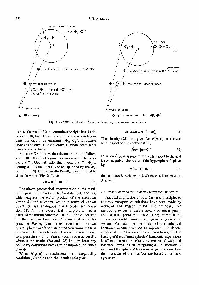
as shown in Appendix A. This result is illustrated in (Fig. 2(a)). The maximizing of/Q(6b, ~) in the identity (25) minimizes the distance of • from (Do. Since the metric is positive definite the identity (25) gives the maximum principle
B((k, ~ ) = 2(D. 2 2 ~ o - ( D <~(Do=/', AS, S>. (26)
The result of maximizing t~'(~b, ~b! for a (D given, in terms of a linearly independent set of vectors (D,,--, ~q~,, d~,~ and nodal coefficients a,, by
N
(D = 3" a,,(D, (27) n = l
is illustrated in (Fig. 2(b)). In applications the set of vectors (D, would for convenience consist of some vectors of the kind {q~,,, 0} and other vectors of the kind {0, d~t}. The minimization of (@-(D0) 2 with respect to the nodal coefficients gives
(a) ( ~ - ~ o ) - ~ , = 0 ] for (n= 1 . . . . . N).
N
a,.(D,.. ~ . = (D.. (D0 ] (28) i.e. (b) m=I
The equations (28) (b) can be solved for the a,, in terms of the source S because there is the formula
(D,. (D o = ( A(divdo,, + £(;b,), S> (29)
142 R.T. ACKROYD
Hypersphere of radius Q R: ~ 1 ~ ) 2
SoLution vector of mognitude <v/~AS, S>
I:~ Approximation vector
C'I 'o- ' I ' )2 + ~ (¢¢) : , I ,~ (2s) ie. QP2+ H (g~,¢)= op2
f space
(a) ~ arbitrary
o ~ Q P 10Q
(30)
r 1 e <'~AS, S >
~:~ : ~a~ (~o confined to Linear N space n:l
~ ~ o f space
(b) (~ optimised eg minimising (~o-~) 2
Fig. 2. Geometrical illustration of the boundary free maximum principle.
akin to the result (24) to determine the right-hand side. Since the O. have been chosen to be linearly indepen- dent the Gram determinant [O,, . 0 . ] , Lancaster (1969), is positive. Consequently the nodal coefficients can always be found.
Equation (28a) shows that the error, or out of kilter, vector 0 - 0 0 is orthogonal to everyone of the basis vectors O,. Geometrically this means that 0 - 0 o is orthogonal to the linear N space spanned by the O,, (n = 1 , . . . , N). Consequently O - • o is orthogonal to • as shown in (Fig. 2(b)), i.e.
( o - 0 o ) . • = 0. (30)
The above geometrical interpretation of the maxi- mum principle hinges on the formulae (24) and (28) which express the scalar product of the unknown vector • 0 and a known vector in terms of known quantities. An analogous result holds, see equa- tion (72), for the geometrical interpretation of a classical maximum principle. The result holds because for the bi-linear functional F associated with this principle F(~b, ~b0) can be expressed as a known quantity in terms of the distributed source and the trial function 4). However to obtain this result it is necessary to impose the condition that ~b is continuous across $1, whereas the results (24) and (28) hold without any boundary conditions having to be imposed, on either ~b orth.
When /Y(~, ~) is maximized the orthogonality condition (30) holds and the identity (22) gives
• 2 + ( 0 - - 0o) 2 = • 2. (31)
The identity (25) then gives for /Y(~b, t~) maximized with respect to the coefficients a.
H(~, ~) = @ 2 (32)
i.e. when/Y(~b, ~) is maximized with respect to the a. it is non-negative. The radius of the hypersphere R, given by
R 2 = ( 0 - 00) 2, (33)
then satisfies R 2 ~< 0o 2 = (AS, S) the case illustrated in (Fig. 2(b)).
2.5. Practical application of boundary free principles Practical application of boundary free principles to
neutron transport calculations have been made by Ackroyd and Wilson (1985). The boundary free method provides a simple means of using parity angular flux approximations t~+(r, fl) for which the dependence on ~ is varied from region to region of the system. For example the order of the spherical harmonic expansions used to represent the depen- dence of (# + on f l is varied from region to region. The linking of the different spherical harmonic expansions is effected across interfaces by means of weighted interface terms. As the weighting at an interface is increased the spherical harmonic expansions used for the two sides of the interface are forced closer into agreement.
A least squares principle 143
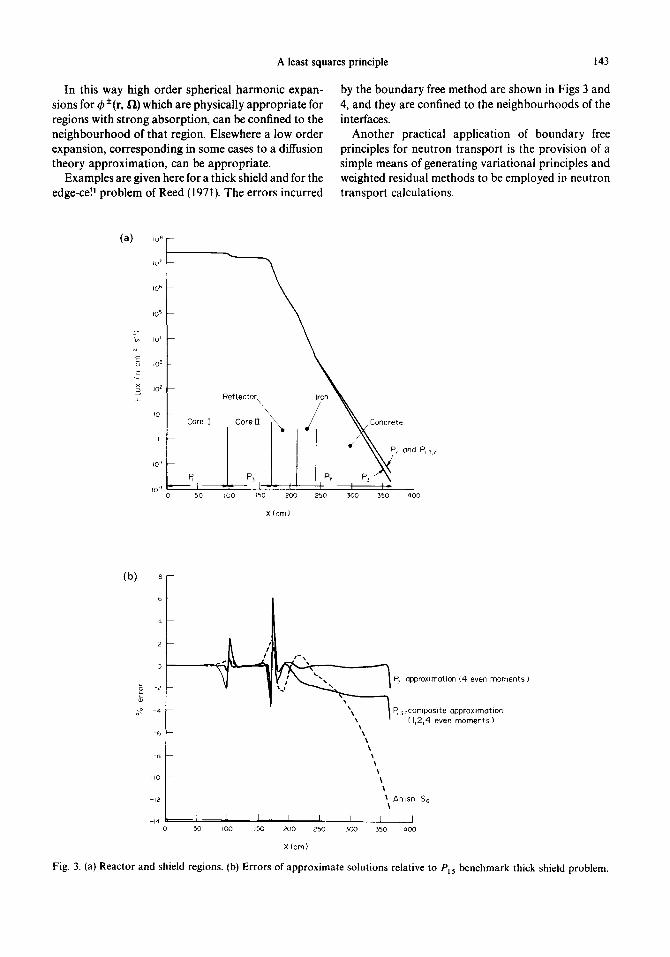
In this way high order spherical harmonic expan- sions for ~b +(r, fl) which are physically appropriate for regions with strong absorption, can be confined to the neighbourhood of that region. Elsewhere a low order expansion, corresponding in some cases to a diffusion theory approximation, can be appropriate.
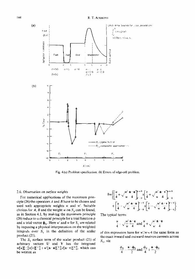
Examples are given here for a thick shield and for the edge-cel I problem of Reed (1971). The errors incurred
by the boundary free method are shown in Figs 3 and 4, and they are confined to the neighbourhoods of the interfaces.
Another practical application of boundary free principles for neutron transport is the provision of a simple means of generating variational principles and weighted residual methods to be employed in neutron transport calculations.
a ) ,u a
io z
106
io 5
I° I -- 7 E o Io 5 -- c
IO 2 -- L~
PO - -
I - -
iO-i - -
fO I
ector\
Core[ C o r e I ] ~ ~ ~, ~ , ~ i : e o n d p .....
P' _1_ P" ,J= I I,P, P , ~ \ I , I I ~ I
50 tO0 150 200 2bO 300 350 400
X(cm)
( b ) 8
2
0
$
4
-4
-i0
-12
- , 4 I ,~ I ,, 0 SO I00 I§0
Pz approximation (4 even moments )
P~,s,z composite a p p r o x i m o t i o n
( 1,2,4 even moments )
Amsn $6
I I I L I 200 250 300 350 400
X(cm)
Fig. 3. (a) Reactor and shield regions. (b) Errors of approximate solutions relative to P15 benchmark thick shield problem.
144 R.T. ACKROYD
(a)
I- I.UX qS(x)
Fue[ I CLodl
2 3
0-:50 o-=5
S : 5 0
Void -~
2 i , ~ 6 x 8
a : 6 c~=l c~:l cr:O9 o- :09 S : I
Logo[ e t r o f bounds for .,[dO obsorbtloRs 5
~ dxo,#(x)
: O 78!5U t~)40%
(b) tO - -
8 - -
6
4
2 --
b ~ o
- 2 - -
- 4 - -
- 6 - -
- I 0
0 /
- - P~ approximabon . . . . P s composite opproxlma-, ,,
P~ P, P~ I , , - ~ I I t - J : I - - =! I 2 3 4 5 6 7 8
X{cm)
Fig. 4.(a) Problem specification. (b) Errors of edge-cell problem.
2.6. O b s e r v a t i o n on surface we igh t s
For numerical applications of the maximum prin- ciple (26) the operators A and B have to be chosen and used with appropriate weights w and w'. Suitable choices for A, B and the weight w on S 2 can be found, as in Section 4.1, by making the maximum principle (26) reduce to a classical principle for a trial function q5 and a trial vector ~0- Here w' and w for S~ are related by imposing a physical interpretation on the weighted integrals over S[ in the definition of the scalar product (21).
The S~ surface term of the scalar product (21) of arbitrary vectors U and V has the integrand
r + O , r + 0 , r + 0 r 4 - 0 • V ] r O, U ] r _ o X [ n c a n w[u]r_oX[V]r_o+W [ n • w h i c h
b e w r i t t e n a s
f l u w' n • u ~r+° r-v / w ' n • v ] r+° , / x - w 4 jr ota+, w 4 j , o n ' u ] ' + ° [-v w ' n ' v , +o
The typical terms
u . w ' n • u u . w ' n " u - ' / w -~ and ~ + , /w
of this expression have for w ' / w = 4 the same form as the exact inward and outward neutron currents across $1, viz
o n'¢o q~o n • ~0o and + - - - - 4 2 2
A least squares principle 145
respectively. Thus for
W' - - = 4 (34) W
the definition (21) for the scalar product U- V becomes
U. V = (A(divu + Eu), divv + Ev)
+ (B(u + DVu). (v + DVv))
+8 w 4+ - - x -+ , 2 J,-o L 4 ~ - ~ - o ..1
2 Jr_o L 4 - - 2 - ,_o
+ ~ w[u--~2n - II][v--~2n - v] dS. (35) .) s 2
Using the revised definition (35) of a scalar product the identity (25) holds for the following special case of the definition (15) for/q(~b, 0), viz
)" <Adiv0, div0> + (AXq~, X~b> f l (¢ , 0) = -- [ + ( s o " 0 ) + (BOVdp " OV~b) J
2~'(Adiv0, X~b) + (B0" DV~b)'~ - [ - (Adiv0, S ) - (AXq~, S) J
fs f/F¢ n'0-lr+°", 2 - 8 w + - - , 4 2 Jr-O)
n - 0 r + o 2
- ~ w(q~-ct2n • 0) 2 dS (36) ds 2
The intermediate results (22)-(25) and the variational principle (26) also hold with the revised definition (35) for scalar product and the revised definition (36) for
0).
3. S O M E W E I G H T E D R E S I D U A L M E T H O D S
D E R I V E D F R O M T H E B O U N D A R Y F R E E
P R I N C I P L E
3.1. Generalized weighted residual method
The vector @ approximating the solution vector @o has the representation (27). The coefficients a, for can be determined from equations (28) and (29). These equations can be recast in the form of weighted residual equations. Particular cases are weighted residual equations of the Galerkin and Petrov- Galerkin types. These are obtained for particular choices of the operators A and B and the weight w which are used subsequently to obtain classical variational principles from the boundary free prin-
ciple. A more general weighted residual method is obtained for A arbitrary. Thus in decreasing order of generality we have the boundary free principle, weighted residual methods with arbitrary weighting A, Petrov-Galerkin methods, and on a par Galerkin and classical variational methods.
From equations (28) and (29) one obtains using the scalar product (21) the weighted residual equations
0 = (div0 + Z¢ - S, A(div0. + Z~b.))
+ (B(0 + DVO). (0. + OV~b.))
f S r+O r+O + {wE¢],_oX[¢.],_o 1
+w'[n- 0]~+°x[n • 0.]~ +°} dS
-]"- r W[~- -~2n" 0"][~)n--(~2n " 0n] dS (37) .) s 2
3.2. Galerkin method
For the particular allocation of weights and opera- tors given in Section 4.2, viz
1 A = E-1 , B = D - l and w = ~ on S2, (38)
the weighted residual equations (37) reduce for the choice of trial function and trial vector
0 = 0 (39)
th. and ~b continuous across S l (40) to
o = .)v {¢.(x¢- s~
+ DV~b,, • V~b} d V
+ [ dp,c~ dS/ot 2. (41) js 2
On using the divergence theorem the result becomes
0 = .Iv <p,(-divOV~b + E~b- S) dV
fS DV~b]r + o dS + ~n[n . r--0 1
+ ~ qS.(q~ + ~tZn • DV~b) dS/a z. (42) j s 2
If the trial function q~ also satisfies the remainder of the boundary conditions, viz
n. DV¢ continuous across $1~ (43) (
4~ + c~2n - DV~b = 0 on S 2 ]
146 R.T. ACKROYD
then the weighted residual equations reduce to the simplest Galerkin form
0 = fv 4 ' , ( -divDV4' + Z 4 ' - S) dV (44)
Here the residual - divDV4' + ~!:4'- S is weighted by the basic function 4'.. In one dimension the optional boundary conditions can be satisfied easily with a finite element representation for 4' which uses a Hermite cubic interpolation over the elements.
The weighted residual equations (42) can be obtained in another way. When a classical variational principle of Section 4 is interpreted geometrically, the weighted residual equations are recovered as in Section 5.
3.3. Petrov-Galerkin method
The choice (38) of weights and operators is retained but the trial function and the trial vector are chosen as follows
(a) The 4', and 4' are continuous across S 1 ~ (45)
(b) ~ , = - D V , with dp= -DV4 ' j
The weighted residual equations (37) become
0 = .Iv (4 ' , -Z IdivDV4',)(-divDV4'+Z4'--S) dV
+ ~ w'[n. r+o r+o DV4']r_o DV 4',]r_ox[n " dS JS I
+ ~ (4 ' ,+~2n. DV4'.)(4'+cdn'OV4')dS,/~ 2. dS 2
(46)
If the optional boundary conditions (43) are satisfied then the Petrov-Galerkin equations (46) reduce to
0 = Q (4'. - Z - 'd ivDV4' . )(- div DV4' + Z4' - S) d V. d *
(47)
Here the weighting used for the residual - div(DV4') + X4' - S is 4', - Z - 1 divDV¢..
For applications the weight w' has to be assigned for the Petrov-Galerkin equations (46). A low value of w' for example exerts little control on n 'DV4 ' at interfaces. As w' is increased the S~ term of equation (46) tends to dominate the character of the solution. The result
lim f w'([n" ,vJ¢'t"lr+°~2-o, d S = 0 , w'~co J S 1
proved below, implies some restriction on the choice of
for high values of w'. For example consider a trial function 4'(x) for a uniform slab, which is represented over each element of the slab by a linear function of x. Then ~ is constant over an element, and in general n. dO= - D d4'/dx is discontinuous at the ends of the element. As w'--* oo the discontinuity in d4'/dx vanishes and 4' has a constant slope throughout. For high values of w' linear elements for 4' are clearly unsuitable.
Solving equation (46) is equivalent to determining the 4' which maximizes/1(4', ~). The result (32) shows that the maximum value of/4(4', ~) is non-negative. The identity (15a) shows that 0<ft(4 ' ,d0)< ( Z - 1S, S), implying
fs w,([ n , . o 2 "~lr O) dS<<X- 'S ,S ) . I
Consequently [n r+o "d0]r_o~0 as w'~oc.. Thus high values of w' tend to enforce continuity of n.dp at interfaces. Trial functions 4' which permit this local tendency without a marked influence on the overall behaviour of 4' are desirable for moderately high values of w'. This difficulty can be avoided for slab systems by using Hermite cubic interpolations over the elements, so that the first of the optional boundary conditions (43) is satisfied.
3.4. Arbitrary weighting
If the operator A is not restricted to the choice (38) and the optional boundary conditions (43) are satis- fied, the weighted residual equation (37) becomes for the substitution (45)
fv 0 = #J ( -d ivDV4' + Z 4 ' - S) d V=0 (48)
for ~O. = A(Z4',-- divDV4'.).
The above examples illustrate how the method of least squares leads to a variety of weighted residual methods on making particular choices for 4' and dO. In the next section classical complementary variational principles are obtained by selecting 4' and ~ appropriately.
4. A CLASSICAL MAXIMUM PRINCIPLE
4.1. Derivation
To obtain a classical maximum principle consider the vector
~.- ,{ 4', ~bo} (49)
with no boundary conditions for 4' specified at present instead of the more general vector ~*--*{4', ~}. A measure of the goodness of the approximation vector
is ( ~ - @ o ) 2. Define for convenience the vectors
A least squares principle
o',-.{4', 0}l (50) Oo.-,{4'o, 0} j
then O - O o = O ' - O o (51)
In obtaining the classical principle the operators A and B and the weight w on S 2 have to be chosen in a suitable way, which leads to the selection (38). The identity
2 0 ' . • o - ( O ' ) 2 + ( O ' - O o ) 2 =
( 0 o ) ~ = (AX4'o, X4'o)
+(BDV4 '°" DV4'°) I +w4'~ dS (52) 'is2
can be used to formulate a maximum principle
2 0 ' . O o - ( O ' ) 2 <(0o) 2 {53)
provided the left-hand side of this inequality is made independent of 4'0. The definition (21) for the scalar product and the boundary condit ion (3a) for 4'0 give
O ' . • o = (AZ4', Z4'o) + ~ w4'4' o dS .)s 2
+ (BDV4' ' DV4'o) (54)
By definition
(0 ') 2 = (AE4', X4') + (BDV4'. DV 4')
+ W([-4']r o) d S + .,4'2 dS (55) 1 2
Thus to obtain a variational principle one has to impose some conditions so that 0 ' . O o is independent of 4'0. On using the diffusion equation (1)
O' • O o = ( A E 4 ' , S ) - (AN4', d ive , )
- (BDV4'. d#o ) + ~ w4'4' o dS (56) 'is 2
If one takes
AE = BD = I (57) then
°" °°=<4" s>- fv div(4"t'o) dV + w4'4'° dS
Consequently the divergence theorem can be used to give
O' • O o = (4', S) ~ [4'n r+o - - . ( l ) 0 ] r _ O dS .Is t
+ 1" 4'(w4' o - n " ~bo) dS (58) 'is 2
147
The independence of 0 ' • • o of 4'0 can be achieved if one takes
4' continuous across S l (a ) ]
1 }" (59) w = ~2-- on S 2 (b)J
for then 0 ' • • 0 = (4', S). The condition (59a) and the boundary condition (3b) make the integral over S 1 vanish. The condition (59b) and the boundary condi- tion (4) ensure the vanishing of the integral over S 2. The inequality (53) can be regarded as a variational principle when the conditions (57) and (59) are imposed.
The variational principle can be obtained alterna- tively be defining a suitable functional. The connection between the two methods can be seen by defining a bi- linear functional /7(0, ~), for arbitrary admissible functions 0 and 4, by
¢)= fv {VO +OX¢} dv + fs. O~ dS/°t2
(60) then for the conditions (57) and (59)
(0') 2 = F(4', 4,), (a)
(Oo)2 = F(4'o, 4'o), (b) ~> (61)
0 ' - • o = F(4', 4'0) = (4), S). (c) .J
The identity (52) can be seen to be an equivalent form of the identity
2F(4', 4"0) - F(4', 4') + F(4' - 4'0, 4' - 4'0) = F(4'o, 4'0)
(62)
Since F(4' - 4'o, 4' - 4'o) is positive definite the identity (62) leads to the K'(4') maximum principle. The functional K'(4') is defined for any admissible function 4', not necessarily continuous across S t by
K'(4')=2(4' , S>-/~14', 4') (63)
In the present application 4' continuous across $1, and the variational principle can be written either as
K'(4')=2<4', S>-F(4 ' , 4')<F(4'o, 4'o)=(~o) 2 (64)
o r
K ' ( 4 ' ) = 2 ( i ) ' • Ii[10 - - (~][~,)2 ~_ ( ( i ) 0 ) 2 ( 6 5 }
This principle in a more familiar form states that for 4' continuous across S~ the maximum value of
K'(4') = fv 124'S-- D(V4') 2 - 224' 2 } d V
- ~2 dS--< q~o 2 (66) 2
148 R. T. ACKROYD
is achieved when 0 = 0o. Generalizations of this kind of principle valid for the even and odd parity transport equations have been given by Ackroyd (1975) and (1978). They were derived there by using appropriate generalizations of the bi-linear functional F. Subse- quently these principles and others have been obtained by Ackroyd, (1982) and (1983), by the least squares method.
because the weights w and w' have no significance for the vector O'*--*{0, 0} and ~0~{00,0} used in deriv- ing the classical principle. In the sequel the scalar products associated with the boundary free principle are of the kind (68). By using the same scalar product a common measure, viz the distance of the approximat- ing vector from the solution vector, is available for comparing various variational methods.
4.2. Essential boundary conditions and the allocation of weights
The boundary condition 0 continuous across S 1 is essential, because it has to be imposed to obtain the classical variational principle (66) by making F(0 , 0o) independent of 0o. In the construction of the bound- ary free principle (26) the scalar product ~o " ~ plays a role analogous to that ofF(0, 00) in the derivation of the boundary tied principle (66), but the former principle is boundary free because the formula (24) holds without any boundary conditions having to be imposed on ~.
A problem in applying the boundary free principle lies with appropriate allocation of weights and opera- tors. Some restriction on A, B, w and w' can be achieved by taking
AE = BD = w(°nS2) - 1. ( 6 7 ) ~2
The classical principle (66) and the boundary free (26) then share the same function space with scalar product
U. V = ( E - t(divu + Eu), divv + ~2v)
+ (D - X(u + DVu). (v + DVv))
S r + 0 r + 0 + {wEu],_oxrv]r_o t
+w, En. uqr+Oxr n . ¢lr+ot dS Jr--O k "Jr--OJ
+ f [ u - ~ = n ' u][v-0cZn.v] dS/~Z)(68) ds 2
4.3. Geometrical interpretation
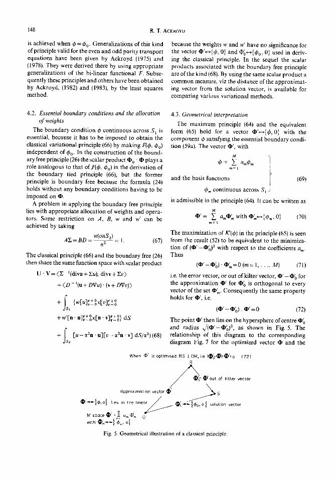
The maximum principle (64) and the equivalent form (65) hold for a vector ~'*--*{0, 0} with the component 0 satisfying the essential boundary condi- tion (59a). The vector O', with
and the basis functions
O,. continuous across S 1
0 = Y a.0., ~n=l
(69)
is admissible in the principle (64). It can be written as
M
• ' = ~ a , ,~ , with ~,*-*{0,,, 0} (70) m = l
The maximization of K'(0) in the principle (65) is seen from the result (52) to be equivalent to the minimiza- tion of ( ~ ' - ~ o ) 2 with respect to the coefficients am. Thus
( ~ ' - ~ o ) " ~ . = 0 (m= 1 . . . . . M) (71)
i.e. the error vector, or out of kilter vector, ~ ' - ® o for the approximation ~ ' for ~o is orthogonal to every vector of the set ~ ' . Consequently the same property holds for ~ ' , i.e.
( ~ ' - ~ o ) . ~ ' = 0 (72)
The point ~ ' then lies on the hypersphere of centre ~o and radius ~/(~,_~;)2, as shown in Fig. 5. The relationship of this diagram to the corresponding diagram Fig. 7 for the optimized vector • and the
When ~' is optimised RS lOR, i.e (~o~).(~':o (72) R
~ g - tl)' out of kilter vector
A / pproximotion vector ~ ' _ . ~ S
~ ' - - {gS, o} Lies in the t n n e c r ~ / ~'o-'~.-{~o, o I ~ s o l . u t i o n vector M
M space~;~' =z~ am~'= 0
Fig. 5. Geometrical i l lustration of a classical principle.
A least squares principle 149
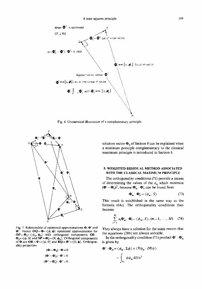
When (~" is optimised T
QT ± RQ / 1 ~
(I)o- t~" out cf kilter vector
SokuUon vector
Approximation vector ~"
(~ ' ' - "10' ~ I ties in the Lineor P s p o r e ~ \
, P . \ e : ~ oeo wt~0---{o,~0l \\
\
2 Fig. 6. Geometrical illustration of a complementary principle.
0
T
o
Fig. 7. Relationship of optimized approximations ~, ~ ' and tb". Vector OQ=O,---,{q~, ~p} optimized approximation for OP=~o,--,{~bo,~Po } with orthogonal components OS= • o,--*{~b, 0} and SP =Oo*--,{0, ~o}. Orthogonal components o f ~ are OR =~',---~{~, 0} and RQ = ~"*--~{0, d~}. Orthogon- ality properties
( ~ - e o ) " • = 0
( * ' - e o ) . ®' = o
(®"- oo ) . e - = o.
solution vector ~o of Section 8 can be explained when a minimum principle complementary to the classical maximum principle is introduced in Section 6.
5. WEIGHTED RESIDUAL METHOD ASSOCIATED WITH THE CLASSICAL MAXIMUM PRINCIPLE
The orthogonality conditions (71) provide a means of determining the values of the a,. which minimize (q~ ' -~o ) 2, because ~ , " ~o can be found from
~ , " ~o = (~bm, S> (73)
This result is established in the same way as the formula (61c). The orthogonality conditions then become
M a t ~ , - ~'~= (q~m, S>, (m= 1 . . . . . M) (74)
/=1
They always have a solution for the same reason that the equations (28b) are always solvable.
In the orthogonality condition (71) product ~ ' . ~ is given by
1~1'" (1)m : <~bm, ~(J~> "q- <V~m" DV(~>
+ js[2 4~¢~ dS/= 2
150 R.T. ACKROYD
Thus the orthogonality condition gives the weighted residual equations
O= .Iv {V49,~ • DV49+49,.(Z49-S)} dV
+ ~ 4949,, ds/a 2 (m = 1 . . . . . M) (75) ,)s 2
On using the divergence theorem these equations become
O= .Iv 49m{-div(DV49)+ Y49- S} dV
+fs [49ran r-0 • DV49]r+o dS 1
-}- f 49m(49 "[- ~2n" DV49) dS/~ 2, (m = 1 . . . . . M) ,js 2
(76)
i.e. weighted residual equations with Galerkin weights 49,.. Furthermore for a trial function 49 which also satisfies the remainder of the diffusion boundary conditions, viz
n • DV49 continuous across S 1
49-t-~2n • DV49 = 0 on S 2
the weighted residual equations reduce to the classical Galerkin equations
0 = Q 49.,{ - div(DV49) + E49 - S} d V (m = 1 . . . . . M)
(77)
6. A MINIMUM PRINCIPLE COMPLEMENTARY TO
THE CLASSICAL MAXIMUM PRINCIPLE
6.1. Need for a complementary principle The classical maximum principle (65) minimizes the
generalized least squares error x / (O ' -Oo) 2. For an approximating vector of the kind O'+-*{49, 0) the generalized least squares error is a minimum when 0 ' - • o is orthogonal to ¢lD'. This property determines O' and it also implies that
F x / ~ o , 490)- F(49, 49)= 4 ( O o ) 2 -- (O') 2
= x/((l)o--O')2 > 0 (78)
Consequently, if an upper bound to F(49 o, 49o) i.e. (O~)) 2 is provided, a measure of the overall goodness
x / ( O ' - @ ' ) 2 of the approximation O' for • o is available.
The provision of an upper bound to (0o) 2 leads not
only to a measure of the overall goodness of the approximation 49 for the exact solution 49o, but also to effective bounds for a local characteristic of 490. A typical local characteristic is the absorption rate in a small locality of a system. A bi-variational method of bounding a local characteristic of neutron transport has been described and applied by Ackroyd and Splawski (1983). The same method can be used for diffusion theory. Here a simpler use is made of upper and lower bounds in Section 12.2 by constructing upper and lower bounds for a global characteristic of a system, viz the absorption probability.
6.2• Derivation A complementary minimum principle is obtained by
considering approximating vectors of the kind ~b.--~ {490, 4} for Oo~{49 o, 40}. A measure of the error made by ~b is ( ~ - O o ) 2, which can be expressed as ( 0 " - 0 0 ) 2 with
o-~{0, 4}
(79) oo~{0, 40}
The scalar products used here and subsequently are defined by (21) with the operators and weights conforming to the conditions (57) and (59b).
The strategy is to use the identity
2 0 " . Oo - (O")2 + (O" - Oo)2 =- (Oo) 2 (80)
with the fact that 0 " - 0" o can be made independent of 4o to derive a maximum principle for (0") 2 approxi- mating (Oo) z, viz
2 o " . • o - ( o " ) 2 __<(Oo) 2 (81)
This principle is then transformed into a minimum principle for ((!)o) 2 with the aid of the result
(o0)2+(Oo)2=(~: 's, s)=OoL (82)
To prove this result note that the specifications (2), (3) and (4) of the diffusion problem give, via the divergence theorem,
O 0 . ( O o - O ~ ) = 0 . (83)
Hence with the aid of the result (23)
( Z - ' S , S) =0o2 =(0o)2 + ( 0 o - - 0 o ) 2, (84)
but according to the definitions (50) and (79)
Oo-O0=og. (85)
Consequently the result (82) holds and the orthogona- lity condition (83) becomes
• o • • o = 0. (86)
A least squares principle 151
To justify the above remark that the inequality (81) can be regarded as a variat ional principle one has to show that 0 " • • 0 is independent ofd~o. Evaulat ing 0 " . • o, by means of the specifications (2)-(4) of the diffusion problem and the divergence theorem, gives
O " . O ~ = (divdp, Z - 1 S ) + ~ [(~o n " '~'lr+° d S v a r - o (87) j s 1
Hence on restricting (~ by imposing the boundary conditions
n. dp is continuous across S 1 (88)
the scalar product 0 " - 0 " is made independent of ~bo, i.e.
0 " . • 0 = (dive), Z - 1 5 ) . (89)
The identity (80) then yields a maximum principle, which can be written as
K"(d~) = 2 0 " . • o - ( O " ) 2 < (O~) 2. (90)
Note that equality holds in this result if, and only if, ( 0 " - 0 o ) 2 vanishes. Since the metric is positive definite equality is obtained for the maximum prin- ciple if, and only if,
dp=~o. (91)
The maximum principle (90) can be recast as a minimum principle, because on using the relationships (80) and (82)
((1)o) 2 + (00) 2 = (Y - IS, S ) - K"(dp) = E"(~) (say). (92)
This result and the statement (65) give the brackett ing bounds
K ' (~b)<(Oo)Z<(Z-~S , S ) - K " ( O ) = E " ( ( I ) ) (93)
provided by the maximum principle K'(q~) and the complementary minimum principle E"(d0).
6.3. Essential boundary condition
It has been necessary to enforce the boundary condit ion (88) to obtain the minimum principle
(~"~ - l S , S ~ - K~'(ID) _ ~_ ( 0 0 ) 2, (94)
i.e. the boundary condit ion (88) is essential for this principle. Whereas the essential boundary condit ion (59a) of the maximum principle (65) requires the continuity across S 1 of the trial flux ~b, the essential boundary condit ion for the minimum principle of (92) demands the continuity of the trial net current vector ~p.
The functional E"((I) ) in equation (92) written in full is
E"(~) = ( Z - ' (d iv~ - S), div~ - S ) + ( D - 1(I)- ~D)
+ f ~2(n' ~b) 2 d S (95) 3s 2
This expression can be used as the definition of E"(d~) for arbi t rary ~. When n • d# is continuous across $1 the minimum principle E"(dp)> (00) 2 holds.
6.4. Geometrical interpretation The vector 0 " ~ { 0 , ~} with
P
* = ~ bp*v p = l
n. ~v continuous across S 1
(a) 1 ?- (96)
(b) j is admissible in the E"(~) principle. It can be written as
P
0 " = ~ bpO~ with ( l ) ~ { 0 , ~p]. (97) p 1
The result (92) shows that the minimization of E"(d~) is equivalent to the minimization of (01)"-01)o) 2 , which gives
(0" - 0 o ) - (!)~ = 0, (p = 1 . . . . . P). (98)
The error vector (0"-0o) for the approximat ion 0 " for O o is or thogonal to every vector (I)~ in the linear P space spanned by the vectors (I)~, (n= l . . . . . P). Consequently
(0" - 0 0 ) . 0 " = 0. (99)
Hence the geometrical interpretat ion given in Fig. 6 for the E"((I)) principle.
7. A WEIGHTED RESIDUAL M E T H O D FOR THE COMPLEMENTARY PRINCIPLE
The or thogonal i ty condit ions (98) lead to a weighted residual method for optimizing a trial vector • of the kind (96), provided some restrictions are placed on the basis vectors ~p. It is assumed that
~ v = -OV~k v, (p= 1 . . . . . P), (100)
i.e. the ~v are conservative vectors. The conservative vector d~ is given in terms of the scalar potential ~k by
P d~=-DV~h= ~-bpDV~hp. (101)
p=l
The approximat ing vector d~ for ~o is related thereby to the scalar ~b in the same way as dp o is related to (ko.
152 R.T. ACKROYD
The result
O; • q)~ = (divdo,, Z tS) (102)
is obtained in the same way as the result (89). The orthogonality conditions (98) become for the scalar product (68)
fv Z -i _ S] - vO } d V divdOp[divdO dO..
+ ~ cdn. dOn - dOp d S = 0 (103) 3s 2
Since-dOp" V0=0divdOv-div(0dO~) the result (103) becomes on using the divergence theorem
v E - ldivdOp[divdo + Z 0 - S] d V
fs EO n ,+o - " do.]r-o dS 1
+fs~ n ' dop(cdn" do-0) dS=0. (104)
For infinite slab system one can put the weighted residual equations (104) in a simplified form. If the 0p are Hermite cubic polynomials then both n • dop and the 0p can be made continuous across interfaces. The boundary condition
~2n "dO = 0 on S 2
can be satisfied also. The weighted residual equation (104) then reduces to
vZ-ldivdOp[divdo+EO-S] d V = 0 1 (105)
with do = - DV0..)
This form of the weighted residual equations (104) bears a strong resemblance to the diffusion equa- tion (2) for ¢0.
One can write (104) in the form
-- fv 52 - l div(DV0p) [ - div DV0 + Z0 - S] d V
fs D~7,/, qr-o dS + [O n. -'epJr +o 1
+ ~ (n-DV0p)(0+ct2n" DV0)dS (106) .Is 2
for the flux approximation 0 derived from the E"(¢) principle. For comparison the flux approximation q~ obtained from the K'(¢) principle satisfies the weighted residual equation (76).
8. GEOMETRICAL INTERPRETATION OF THE K'(~b), E"(~b) AND A(~, ~b) PRINCIPLES
8.1. Equivalence of the combined use of the K'(4~) and E"(do) principles with a form of the H(49, do) principle
A geometrical interpretation of the boundary free /l(~b, dO) maximum principle has been given in Sec- tion 2.4. Similar geometrical interpretations of the boundary tied K'(4~ ) and E"(dO) complementary prin- ciples have been given in Sections 4.3 and 6.4 respec- tively. When 4) is admissible for the K'(~b) principle and dO is admissible in the E"(dO) principle the maximization of IZI(¢, dO) gives the same result as the maximization of K'(q~) and the minimization of E"(do), provided the trial function q~ and the trial vector dO are chosen indepen- dently, and the operators A and B for/q(¢, do) satisfy the condition (57). With this choice of A and B the same scalar product (68) is used to interpret geometri- cally the K'(¢), E"(do) and H(¢, dO) principles. The identity (25) is then
/)(~b, d o ) + ( ~ - ~ o ) 2 = O ~ = ( E - 1 S , S). (107)
Instead of considering vectors of the kinds ~'--*{¢0, dO} and ~ { ~ b , dOo} as approximations for Oo,--,{q~0, dO0}, as is done in deriving the E"(dO) and K'(q~) principles respectively, ~,--.{¢, dO} is taken as an approximation for • 0 for optimization by the/4(¢, dO) principle.
Associated with the trial function ~b for the K'(4~) principle, as defined by (69), there is the trial vector O' given by the definition (70). Similarly for the trial vector dO for the E"(dO) principle there is the vector ~" given by the definition (96). For the/t(¢, q~) principle ¢ and dO define the vector
O=O'+O"M P } with O = Z % 0 " + ~ b,O;. (108)
m = l p = l
The identity (107) shows that the maximization of /t(~b, dO) is equivalent to the minimization of(@ - O0) 2. Minimization with respect to a,, gives
(O-O0)" O~,=0 tin= 1 . . . . . M) (109)
and minimization with respect to bp gives
(O--q~o) • O ; = 0 (p=l . . . . . P). (110)
To simplify these results the properties of vectors of the first and second kinds given in Appendix B are used. Generally a vector of the first kind U', (say) is U'*-+{u, 0}, and a vector U" of the second kind is U"*-*{0, u}, and any vector U~--,{u, u} has the resolu- tion U = U ' + U " . In the result (109) 0 - 0 0 can be resolved into the components 0 ' - 0 o and O " - O o.
A least squares principle
By property (B4) of Appendix B the latter component of O - • 0 is orthogonal to O;.. Thus
( 0 ' - 00). 0;. = 0 t (m=l . . . . . M). M
i.e. ~ a,0'~ . 0 ; . = 0 ; . . 0 ' o I = 1
(11l)
These equations for the coefficients a t are identical with those given by the results (73) and (74) obtained independently by maximizing K'(4'). Similarly the result (110) can be written as
(0" - Oo). 0~;= 0 ]
e I ( p = l . . . . . P). (112) i.e. ~ b¢O~' O~=O~' O" 0
q = l
These equations for the coefficients bq are identical with the equations (98) obtained independently by minimizing E"(do). The equivalence of the H(4', do) principle to the combined use of the K'(4') and E"(do) principles is thus established for the conditions stated above.
When 4' and do maximize H(4', do) the functional h'(4') is maximized and E"(do) is minimized, and
h ' ( 4 ' ) + ( O ' - 0 o ) 2 + ( O " - 0 o ) 2 = E"(do) (113)
holds. This result follows from the definition (92) and the result
K'(4') + (O ' - -Oo) 2 =(00) 2 (l 14)
the consequence of the identity (52) and the definition (65). Since 0 ' - 0 0 is orthogonal to 0 " - 0 0 by property (B5) the result (113) can be written as
K'(4') + K"(do) + ( O - O o ) 2 = (X - iS, S ) = 0 o 2 (115)
on recalling the definition (92) for K"(do). Comparison of(115) and (107) shows that when 4' and d o maximize
/~(4', 4,) K'(4') + K"(do) = H(4', do). (116)
8.2. Relationship of the optimized vectors 0 ' , 0" and •
When 4' and do maximize /t(4', do) there are the results (30), (31) and (32), viz
(O- 00). • = 0
• 2 + ( O - O o ) 2=O~ I (117)
~(4', 4,) = 02. Since 4' then maximizes K'(4') the results (52), (72) and (114) give
153
(o'- Oo)- o' = 0 1 1
(0')~ +(o'-Oo)~ =(Oo) ~ ~ (118) h~(4')=(o')~. ~
Since do then minimizes E"(do) the results (80), (90) and (99) give
(o"-Oo). 0o =0
(0") 2 + (0" - Oo) 2 = (@°)2 I (119) K"(do) =(O") 2 .
The last members of the results (117)-(119) and the relation (116) give
(0') 2 +(0") 2 = 0 2 . (120)
Since 0 ' and O" are vectors of the first and second kind respectively
O' • O"=0. (121)
The results (109) and (110) give
( 0 - 0 0 ) - O'=0 t ~ ( O - O o ) . 0 = 0 (122)
(0-00)" 0"=0 The properties (117)-(122) of the optimized approxi- mations 4' and • are illustrated in Fig. 7. The solution vector • o has orthogonal components • o and • o. The optimized approximation • for • o yielded by the /~ principle has orthogonal components O' and 0" given by the K' and E" principles.
9. FINITE DIFFERENCE SCHEMES FOR FLUXES
9.1. General remarks on.flux and current schemes
The K'(4') principle is used in this section with a finite element representation for the flux 4' to derive finite difference schemes for one and two dimensional systems. In Section 10 the K"(do) complementary principle for the net current do is used to obtain finite difference schemes for one and two dimensional systems. Here it is helpful to anticipate the ways in which the flux schemes of the K'(4') principle and the current schemes of the K"(do) principle differ.
For simplicity the source S is taken to be a constant within an element. For one dimensional systems there is a node at each end of the element for both the flux and current schemes. The finite element used for the two dimensional flux scheme employs a node at each corner of the element, whereas for the current scheme the nodes are at the mid-points of the sides. There are two variants of the current scheme. In the first scheme there is no restriction on the components of do, and as a
154 R.T. ACKROYD
consequence there are for two dimensions two differ- ence equations in place of the single difference equation of the K'(~b) and classical schemes for the flux.
At first sight the extra complexity of the K"(~b) scheme for two dimensions suggests that the scheme is of academic interest only. In Section 11 the vector d~ is constrained to satisfy the conditions:
(a) dp is the gradient of a scalar if, (b) dp and ~ satisfy the conservation condition for
each element.
These constraints can then be used with the two difference equations of the K"(d~) scheme to obtain a nine-point difference equation for the average fluxes for the elements. Special cases of this scheme give difference schemes of the nodal* type for one and two dimensions. The corresponding analysis for a K'(qS) nodal scheme is then given. Surprisingly the nodal equations for the average flux 05 have exactly the same form as the nodal equations for if, although the variational principles employed and the finite elements employed in the two derivations are different.
The principal features of the K'(tk) and K"(d~) are given in Table 1. The schemes (a}-(e) relate the values at the element nodes of the continuous variables ~ and ~, whereas the schemes (f)-(j) relate the values for the nodes or elements of the discontinuous variables and 05.
The nodal equations derived here by the finite element method are restricted to expansions for the fluxes which are quadratic in the local coordinates of the finite elements. They therefore should be compared with the zeroth order form of the conventional nodal methods. The finite element analysis given here can be extended using higher order representations for ~b or ~b as appropriate, to give higher order forms of the nodal method.
The conventional nodal methods, which have been developed by Wagner (1975), Dorning (1979) and Putney (1984), represent the flux in each node, or element, by a polynomial expansion. The coefficients of the polynomial are determined using a combination of weighted residual equations and continuity condi- tions. There are several variants of the conventional nodal method--the point flux and the average flux schemes, and the point current and average current procedures. Here we give finite element analogues of
the conventional average flux and average current nodal schemes.
Nodal methods use a nodal balance equation for each node, or element, to relate the average flux in the node to either the average fluxes or partial currents on its surfaces. These surface averages describe the coupling of adjacent nodes or elements. The surface flux/current equations can be used to express the surface fluxes/currents in the nodal balance equation in terms of the average fluxes in the node adjacent to the surfaces of a designated node. In this way an equation is obtained for the average fluxes of the node having a structure similar to that of the classical mesh-centred finite difference diffusion equation. The coefficients in this nodal equation are dependent on the nodal fluxes and surface fluxes/currents, and they therefore have to be determined by some form of an interative scheme.
The nodal equations derived by the finite element method for the average fluxes are similar in structure to the classical finite difference equations for point fluxes. Whereas the coefficients in the nodal equation of the conventional nodal method have to be deter- mined interatively, the coefficients for the nodal equations of the finite element method are given directly in terms of the nuclear data.
Some reactor physicists believe that finite element methods are unsuitable for efficient coarse mesh schemes for regular meshes. One reason given is that the number of unknowns used in a finite element specification is too large, because of the continuity conditions imposed between elements. The resulting equations for a regular mesh have a more complicated structure than the classical finite difference equation, and this has been regarded as an impediment to their efficient solution.
The finite difference equation derived from the K'(qS) and K"(d~) principles with the aid of the finite element method do have a more complicated structure than the classical finite difference equations. However the coefficients in these equations can be related to the average fluxes for the elements in such a way that five- point formulae for the average fluxes can be obtained. Since the K'(~) and K"(~) principles give rise to weighted residual methods, it is not surprising that on using polynomial expansions for ~b or d~ within an element that some correspondence can be found between the finite element and nodal methods.
* Since the nomenclature of the nodal method conflicts with that of the finite element method, terms of the former method are given in italics. A node in the finite element method is a specified point of an element, whereas a node in the nodal method is an element. The nodal value of a variable in the nodal method is the average value for the node.
9.2. Three-point scheme for fluxes in one dimension
The local coordinate ~ for the ruth element of length h has the range [ - 1 , 1], i.e. x=xm+~h/2 with x m denoting the coordinate of the mid-point of the element. The nodes of the element are at x,._~ (this

A least squares principle 155
Table 1. Features of finite element difference schemes
Properties Type of scheme
Conservation Variational Continuity Continuity condition for Exact equivalent to the Approximate equivalent to
principle of flux of current elements finite element method finite element method
Yes No No One dimension
(a) Three-point scheme of equation (124) for nodal va- lues of q~
Two dimensions
K'(~b) (maximum) for 4~ flux, ~ aver- age value of q~ over an element
(b) Nine-point scheme of equation (126) for nodal va- lues of ¢ (f) Nine-point nodal scheme of equation (153) for ¢. Ex- act reduction to five-point scheme (154) if element pitches satisfy
hk Diffusion
length
(c) Five-point scheme of equation (130) for nodal va- lues of ~b (g) Five-point nodal scheme (154) for ~b for arbitrary ele- ment pitches
Basic version E"(d~) (mini-
mum) for net cur- rent
No Yes No One dimension
(d) Three-point scheme of equation (133) for nodal component of
Two dimensions
(e) Ten-point coupled differ- - - ence scheme of equations (136), (137) for nodal com- ponents of
Conservative ver- sion
= DV~b . t~ average value
of ~p over an ele- ment
No Yes Yes One dimension
(h) Three-point nodal scheme - - of equation (146) for
Two dimensions
(i) Nine-point nodal scheme of equation (145) for i~. Ex- act reduction to five-point scheme of equation (147), if element pitches h, k satisfy
hk Diffusion
~/6(h2 + h 2 ) length
(j) Five-point nodal scheme of equation (150). This scheme has exactly the same form as the nodal scheme equation (147) for
156 R.T. ACKROYD
choice is convenient for the K"(~b) principle appli- cations of Section 10).
For the K'(4~) principle the trial function ~b for the ruth element is given in terms of the flux nodal values bin+ ½ and b= ½ by
~b={b,.+½+b,. ~ + ( b . , + , - h , . ,,)~'/2 (1231
The source within the element has the constant value S,.. Maximizing K'(q~) with respect to 6,.+½ gives the difference equation
- D(b,.+ ~ - 2b,.+ ~ + b,. ,)/h 2
+ E(b,.+~+4bm+~ +b,. ½)/6
= (S, . + , + S . , ) /2 (124)
Here the absorption term is not as simple as that for the classical difference equation, but the leakage term is the same. In extending the analysis to two dimen- sions both the leakage and absorpt ion terms become complicated.
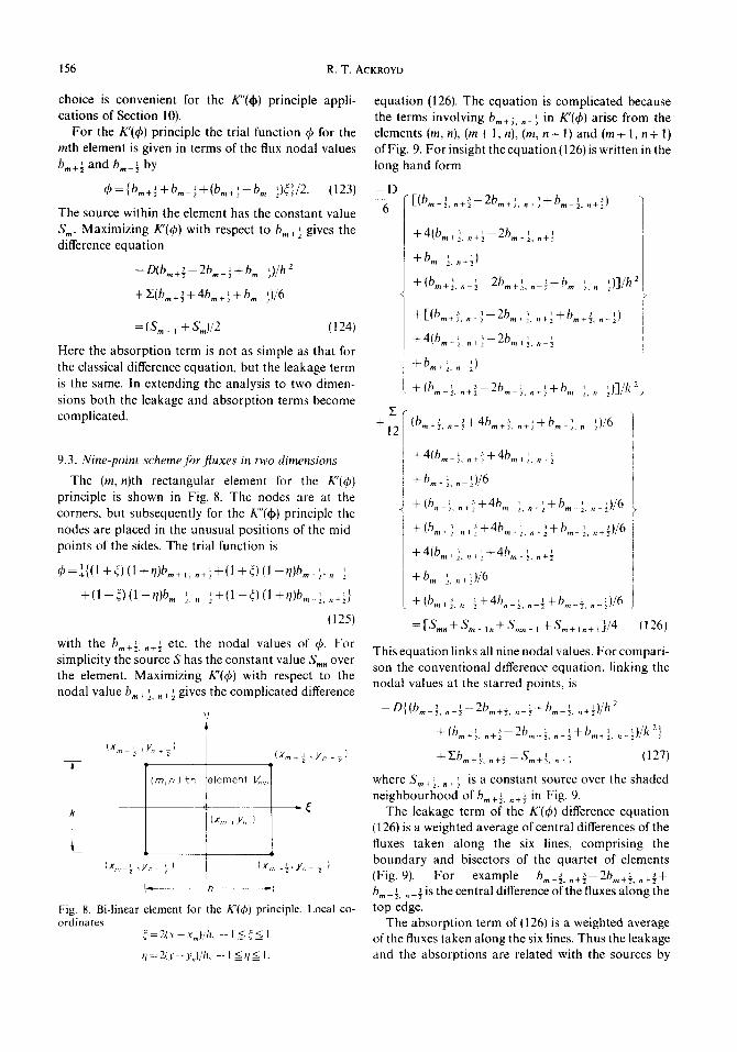
9.3. Nine-point scheme for. f luxes in two dimensions
The (m, n)th rectangular element for the K'(~b) principle is shown in Fig. 8. The nodes are at the corners, but subsequently for the K"(~b) principle the nodes are placed in the unusual positions of the mid- points of the sides. The trial function is
~ = ' { (1 + ~) (1+ ~)bm+,,. +~+(1+ ~) (1 - ~)6.~*F. I
+ ( l - ~ ) ( l - q ) b ~ 1,. ~ + ( 1 - ~ ) ( l + t / ) b . _ } . . . . ~}
(125)
with the bin+½,..½ etc. the nodal values of q~. For simplicity the source S has the constant value Sin. over the element. Maximizing K'(~b) with respect to the nodal value b,. + ~,. +~ gives the complicated difference
(x _ . , y . . + ) / ( x m . - , x . . ~ )
l ' 2 ] (m,n) th lement G~.
I i (Xm , Yn
3_ (x~ ½,y._ ~) (x~+.,y. - )
Fig. 8. Bi-linear element for the K'(40 principle. Local co- ordinates
= 2(x- x~)/h. -- 1 < ~ < 1
~1 =- 2(y- y.)/h, -- 1 < q < 1.
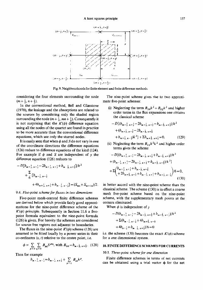
equation (126). The equation is complicated because the terms involving b ~ , in K'(q~) arise from the elements (m, n), (m+ 1, n), (m, n + 1) and (m+ 1, n + 1) of Fig. 9. For insight the equation (126) is written in the long hand form
- D
6
E
+ 12
I b 3 , _ , 3 1 [( ,.+~,.+~ 2b,.+~,.+2+b,._~..+~)
1 + (bm+.,.+~ 26m+2, o+,
+6, . L.+'~)
~-(6m+~,n ~--26m+~... n ~ - 6 m 2; n ~)] /h2 (
+ [ ( b , . , ~ . . , { - 2 b = + ~ , . ~ + 6 , . + ~ , . . ~ ) i
+ 4(bin+ ~,. ~ ~ - 2 b , . , ~, .+ ' q i
+(b,. } , . , ~ - - 2 b . '~,.+'~+/'m '2,. ~)]/k2j
(b=+~,.+~+4bm+~,.+~+bm+~,,, ½)/6
+4(bin+ ' . . +~+4hm+½..+~
+(h . L.+~+46m ' +'+hm_~, ~ ~)/6
+(6~+L.,.~+4b.+; .... }+b~ L.+~)/6
4(b + m ~ . . + ~ + 4 b ' 1 m ÷ : . n * s
+bin ,~,. +})/6
+(hm+J. . '~-F4b.+L. ~+bm. ½. ._.'=)/6
= [ S m n + G + l n + S m n ~ l + S m + , . + l ] / 4 (126)
This equation links all nine nodal values. For compari- son the conventional difference equation, linking the nodal values at the starred points, is
- D{ (bm+ J. .+'~- 2bm+ ½. .+ '2 + 6m '2 . . . . ~2)/h 2
+(bm.~, .+~-26m+ ~, .+':+bin,'2, . . '.)/k 2 }
+ E b . . ~ . . + ~ = S,. ~,2, . ~, (127)
where S.,+~, .+~ is a constant source over the shaded neighbourhood of b , ~ in Fig. 9. m+~, n+2
The leakage term of the K'(q~) difference equation (126) is a weighted average of central differences of the fluxes taken along the six lines, comprising the boundary and bisectors of the quartet of elements (Fig. 9). For example b 3 ~ - 2 h , m+~,n+~ ~m+2, n+~ + bm ~,'. +~ is the central difference of the fluxes along the top edge.
The absorpt ion term of (126) is a weighted average of the fluxes taken along the six lines. Thus the leakage and the absorpt ions are related with the sources by
A least squares principle 157
Im-½,n*~),
! i ", ( r n - z , n +-~) /
i i ( r n - 7 , n -~)
V~n.,
i/ /// H I / / / ~ !/ / / ~
( r e , o )
I/m* t n+ ~
# 2
.77"- 7 q
"(m+g,n +½} / / / / I
h
%o ,b- I I { m + ~ , n - g )
, ( m * ~ , n + ] }
t k
I \ 3 d / (m + 2 , n + 7 )
, 5 r J77 +2 , 0 - ~ }
Fig. 9. Neighbourhoods for finite element and finite difference methods.
considering the four elements surrounding the node ( m + ½, n + ½).
In the conventional method, Bell and Glasstone (1970), the leakage and the absorptions are related to the sources by considering only the shaded region surrounding the node (m + ½, mn + ½). Consequently it is not surprising that the K'(~b) difference equation using all the nodes of the quartet are found in practice to be more accurate than the conventional difference equations, which use only the starred nodes.
It is easily seen that when ~b and S do not vary in one of the coordinate directions the difference equations (126) reduce to difference equations of the kind (124). For example if ¢ and S are independent of y the difference equation (126) reduces to
-D[bm+], .+½- 2b,.+½, n+½-I-bm_½, .+~]/h 2
Z + g [brn+~, n+½
+ 4b,. + ½, .+½+ b.,_ ½, .+~] = (Sin. + Sin+ 1.)/2.
9.4. Five-point scheme for fluxes in two dimensions
Five-point mesh-centred finite difference schemes are derived below which provide fairly good approxi- mations for the nine-point difference scheme of the K'(q~) principle. Subsequently in Section 11.6 a five- point formula equivalent to the nine-point formula (126) is given. For brevity the schemes are considered for source free regions not adjacent to boundaries.
The fluxes in the nine-point K'(¢) scheme (126) are assumed to be fitted locally by a power series in their co-ordinates (s, t) relative to the centre point, i.e.
dp = • Z Bpq Sin, with Boo=bin+½..+½. (128) p = O q = O
Thus for example
b ~ , - b ~ '~- ~ BnohP. m+]Ln+~.-- m+~, n + ~ - - p = l
The nine-point scheme gives rise to two approxi- mate five-point schemes:
(i) Neglecting the term B20h 2 + Bo2k 2 and higher order terms in the flux expansions one obtains the classical scheme
-D{(bm+~, ~ -2b ' b ' ' 2 .+: m+~, .+½+ , .- : . .+:)/h
+ (bin+½, .+~-2bm+½, .+½
+ b ' ._½)ka}+Zb.+~,n+~ 0. m+~, 1 , = (129)
(ii) Neglecting the term B22h 2k 2 and higher order terms gives the scheme
-D{(b.+~_. , - 2 / , , , , .+3 v.+~, .+~+b._:, n+½)/h 2
+tb ~ 3-2/ , ~ ~J-h ~ ._½)/k 2}
+ z / b . +k, .+½+ b.+½, .+~ ~/6 =0, \ + 2bin+{, .+½ + b._½, .+~+bm+½, ._~
(130)
in better accord with the nine-point scheme than the classical scheme. The scheme (130) is in effect a coarse mesh five-point scheme based on the nine-point scheme, with the supplementary mesh points at the corners eliminated.
When ~b is independent of y
--Dth 3 , - g h , '~-b 1 .+½)/h 2 ~ m + ~ , n+~ ~Vm+~, n+~- - m-~,
+ Z(b~+~, .+½+4bin+½, .+½
4 1 , , - + b.+~+bm_~, .+~) /6 -0
i.e. the scheme (130) becomes the exact K'(~b) scheme for a one dimensional system.
10. FINITE D I F F E R E N C E S C H E M E S FOR C U R R E N T S
10.1. Three-point scheme for one dimension
Finite difference schemes in terms of net currents can be obtained using a trial vector ¢~ for the net
158 R.T. ACKROYD
current doo. The vector do can be optimized by minimizing E"(do). According to the result (92) this is equivalent to maximizing K"(do). Using the definition (95) of E"(do) gives
K"(do)=2(E ~S, d ivdo) - (Z-Mivdo , divdo)
- ( D - ' d o ' d 0 ) - f cQ(n. do)2 dS. (131) Js 2
For an infinite slab the trial vector do is assumed to vary linearly over the length h of the elements. For an element with mid-point at %. the trial vector is
do- i ra ~ - a ,+ t , , , - % ~)¢]/2, (132) - - L m + ~ - - r n - E - - ~ , ~ m + ~
where a , and a ~ are the net currents in the x m + ~ m--2
direction for the ends of the elements at x" + ~ and x m_ respectively. The local co-ordinate ~ has the range [ - 1 , l] and x = x " + ~ h / 2 . Maximizing K"(do) with respect to a,.+½ gives
- D [ a " + 3 - 2am+~2 + a " ½]/h2 + Z[a"+3+4a,.+~2
+ a,._ ~]/6 = - DIS,.+ ~ - S,.]/h. (133)
A flux ~k can be associated with the net current dO by making do and ~O satisfy the same conditions as the doo and qfo, viz
do = - DV@ (a) ~]
(I 34) fo [s-z qdV=fo d o . n d S (b)j lement lement surface
Thus in the present example
2 ~ ~ , = A , , - [ (a , ,+~+% ~)~
+ ( a " ~+,--a ,. ~')~2 ]/h8D
with Am=Z ~ [ S , . - ( % + ½ - a , . , ) (1 /h+h/240)] .
Making do and @ satisfy the conditions (134) is the means employed in Section 11 to transform the K"(do) difference scheme of Section 10.2 for two dimensional systems into a scheme for average fluxes. The condi- tions (134) provide the key for relating finite element to nodal methods.
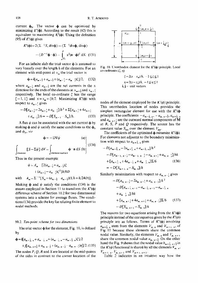
10.2. Ten-point scheme for two dimensions
The trial vector do for the element, Fig. 10, is defined by
do=i[a , .+½. .+a" ½ , . + ( a . , + ~ , . - a " ~,.)~]/2
+j[a . . . . ½+am. . ½+(a . . . . ½-a. , . ._½)q]/2.(135)
The nodes P, Q, R and S are located at the mid-points of the sides in contrast to the corner location of the
T R k - I
Q (rn,n + ~ )
Vmn I
( m - ½ , n ) J (m,n) p
i t
s ( re ,n -½) "t_ I h
Fig. 10. Unorthodox element for the K"(d~) principle. Local co-ordinates (~, t/)
= 2(x -- x.,)/h. -- 1 < ~ < 1
r/= 2(y - y.)/k, - 1 ~ t 1 < 1 i, j = unit vectors.
nodes of the element employed by the K'(~b) principle. This unorthodox location of nodes provides the simplest rectangular element for use with the K"(do principle. The coefficients - a,. _ ~, , , - a,n ' . _ ~-, a., +_~,. and am,. + ½ are the outward normal components of M at R, S, P and Q respectively. The source has the constant value S,.. over the element V,,,.
The coefficients of the optimized do minimize K"(do). For elements not adjacent to the boundary minimiza- tion with respect to am+~,, gives
--D[a,.+~. . - 2a,.+2 ' .+a. ,_~, n]/h 2
1__ . ~ a , . , . + ~ + a , . , . _ ~ ] / h k --O[am+t,n+~ am+l, ~-- ~ 1
+ [%+~, , + 4am+~, . + % _ ½ . . ] Z / 6 (136)
= -- DES,.+ 1 , . - S", .]/h
Similarly minimization with respect to a,., .+½ gives
-DEa. , , . + ~ - 2"a,., .+½ +a.,. ._~]/k 2
- -D[ - a , - a , a m + ½ , n + 1 " ] , n + l m + ~ , n
+ a,,, ½, .] /hk
+[a , . , ~+4a .+½+a,., ._½]E/6 (137)
- - D[ S . . . . 1 - - S . , . . ] / k
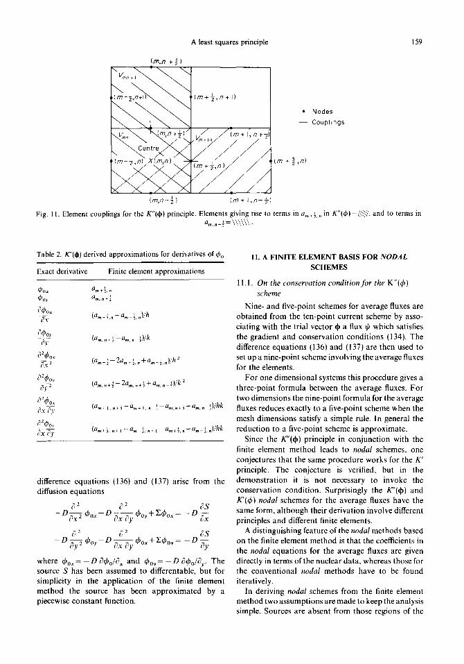
The reasons for two equations arising from the K"(do) principle instead of the one equation given by the K'(¢) principle are as follows. Terms of K"(do) involving a , stem from the elements V, . . and V,.+I.. , of m+~, n
Fig. l l because these elements share the common nodal value. Similarly, the elements V,.,. and V,., .+ share the common nodal value a,., .+½. On the other hand the Fig. 9 shows that the nodal value b,. + ½,. + ~- in the K'(qf) functional is shared by all the elements V".., V " + , , . , V,., .+1 and V,.+l ' .+1"
Table 2 indicates in an intuitive way how the
A least squares principle 159
(m,n + ~ )
(m,n - ½ )
( m + ½ , n + I )
,_~, / /~v, / / Im+i,~+-~;,
I~++,~ /
(m+ I, n - ~-)
• N o d e s
- - Coupl ings
(m + ~ ,n)
Fig. 11. Element couplings for the K"(¢) principle. Elements giving rise to terms in a, .+. . , in K"(O)=/////7. and to terms in a . . . . ½ = \ \ \ \ \ \ .
Table 2. K"(d0) derived approximations for derivatives of ¢o
Exact derivative Finite element approximations
~b0x a t m+1, n (~OY a l m . n + ~
-,77U (a.,+ L . - a , , , ½..)lh
a4)o,. -~7' (a . . . . ½-a . . . . 0/k
¢32~)°x la,.+ ~_ 2am+ ~., + am ', .)/h 2
az ¢--°r (a . . . . ~ - 2a . . . . ½ + a,.. ._ O/k 2 ?), 2
a ,_~ a,. . .+~+ ,.. . O/hk ?x ?y ( =+ ..+~-a,.+,, ,-- , a ,
a2¢o,, (a=+~. ,+ 1 --a,. ~..+l' -a=+~_. n+arn_½..)/hk ¢:X cy
difference equations (136) and (137) arise from the diffusion equations
¢')2 ~ 2 O S
- - D ~ x 2 ¢°~-- D bxfiy ~b°Y+5:¢°~ = - -D
- D ~?y 2 dPoy-- D ~x Of qs°x + Zqs°r = - D Oy
where ~box=- O Oq~o/0 x and q ~ o y = - D dq~0/c~y. The source S has been assumed to differentable, but for simplicity in the application of the finite element method the source has been approximated by a piecewise constant function.
I1. A FINITE ELEMENT BASIS FOR NODAL
SCHEMES
11.1. On the c o n s e r v a t i o n cond i t i on f o r the K"(~) s c h e m e
Nine- and five-point schemes for average fluxes are obtained from the ten-point current scheme by asso- ciating with the trial vector ~ a flux ~b which satisfies the gradient and conservation conditions (134). The difference equations (136) and (137) are then used to set up a nine-point scheme involving the average fluxes for the elements.
For one dimensional systems this procedure gives a three-point formula between the average fluxes. For two dimensions the nine-point formula for the average fluxes reduces exactly to a five-point scheme when the mesh dimensions satisfy a simple rule. In general the reduction to a five-point scheme is approximate.
Since the /C'(~) principle in conjunction with the finite element method leads to noda l schemes, one conjectures that the same procedure works for the K' principle. The conjecture is verified, but in the demonstration it is not necessary to invoke the conservation condition. Surprisingly the K"(d#) and K'(ch) noda l schemes for the average fluxes have the same form, although their derivation involve different principles and different finite elements.
A distinguishing feature of the noda l methods based on the finite element method is that the coefficients in the noda l equations for the average fluxes are given directly in terms of the nuclear data, whereas those for the conventional noda l methods have to be found iteratively.
In deriving noda l schemes from the finite element method two assumptions are made to keep the analysis simple. Sources are absent from those regions of the
160 R.T. ACKROYD
system for which the nodal schemes are obtained. The elements do not abutt the boundary of the system.
Thus
11.2. Nine-point K"(d~) nodal scheme
Within the element V,.. the flux ~b is taken to be
ff(~, q)=~k(0, 0 ) - ~ (a,._½, .+am+½, .)~
+(a, .+½,.-a, . _~,~ . ) ~ }
k 1 a 1
4D {(a,., ._~+ ,., .+Qr/
t/2 - - a 1 +(a . . . . ½ m,.-~) ~-}'
- D ~xx = [(a.,_½, .+am+k, .)
a 1 +( m+~. , -am-½. ,)~]/2 (138)
O e~, Oy = [a,., ._½+am, .+½)+ (am, .+~--a,., ._½)r/]/2.
i.e. these expressions for the net currents are in accord with the expression (135) for the current vector d~. In passing it is to be noted that ~ is an expression of the same kind for the flux as is used in the nodal method, but different means are used by the finite element and nodal methods in determining all the coefficients in the expression for ~.
The K"(#) principle determines the coefficients am+~- ' . etc. in the expression for ~O. To determine ~k(0, 0) the conservation condition for the element Vm. is imposed. If if,.. is the average value of ~, for the element (m, n) is found then ~k(0, 0) can be found. The conservation condition gives
f n . ~b. n d S = - f v . YqJ dV=-Y-hk~m. , (139)
where B,.. is the surface of the volume V,... This conservation condition, viz
k(ar.+ ½" . - a , . _½. .) + h(a,., .+ ½-a,., ._½)= - Zhka . . . . (140)
and the K"(dp) difference equation (136) give
D(~,. + L .--i~,.. .)/h= - [a , .+~, . +4a,.+½.. +am_½, .)/6. (141)
Similarly
D(i~,., .+l - -~m. . ) /k= -(am..+~ + 4a,...+½
+ ar. ' . + ½)/6
The coefficients a , etc. can be eliminated from r a + ~ , n
equations (139), (140) and (141) as follows to give a nine-point equation in the average fluxes. For one dimension this equation reduces to an exact three- point formula; and for two dimensions there is a five- point approximation, which becomes exact for certain element sizes.
Define the displacement operators E~ and E 2 by
Elfpq =fp + 1. q, E2fpq =fp.q +x,.for p = m, m + ½ etc.
q = n, n + ½ etc. (143)
Since these operators commute, the coefficients a , etc. can be eliminated from
m + ~ , n
6D - - - - - - a 1 h2 ( E, 1)~m.= {(E1--I)2+6E,} m ~,./h
6D k ~ ( E 2 - 1 ) ~ , . . = - { ( E 2 - 1 ) 2 + 6 E 2 } a , . , . _ ½ / k (144)
and
(E~ - 1 )a,._ ½../h + (E 2 - 1 )a,., ._ ½/k = - E~m .,
the operational forms of equations (141), (142) and (140). The result is
- D E2 + 6 (E 1-1)2/h2
+ E l + 6 (E 2 - 1 ) 2 / k 2 ~.,,
+3- E ~ + ~ E2+ 6 q~,.. = 0.
(145)
11.3. Three-point K"(d~) scheme
For one dimensional systems E2~,n n = ~ran (say), and then
(E~ - D ( E x - 1 ) 2 ~ m , / h 2 + E { E x + 6 1)2}~m,=0.
i.e.
+E{~,.+2 ' . +4i~m+, ' . + ~.,n}/6 = 0. (146)
This equation resembles the homogeneous version of equation (133).
11.4. An exact five-point K"(#) nodal scheme
For two dimensional systems the difference equa- (142) ' tion (145) reduces to the five-point formula
A least squares principle 161
-DE(q$,. + 2 , . + , - 2 ~ , . + , . .+ , + t~,.,. +,)/h 2
+ (~ , .+ , , .+2 -2~ . ,+ L .+ , + ~m+,, .)/k z]
+ £(~,.+ a, .+, + ~, . , .+, + 2~, .+ , , .+ ,
+ ~.,+ L.+ z + ~, .+, . . ) /6 =0, (147)
provided that the error term
[-6D(~--~+~--~)+E](E,-1,=(E:-I)2~,,,,/36
is negligible. The five-point formula (147) is therefore an exact
deduction from the K"(~) principle provided that
11.5. Approximate five-point K"(#) nodal scheme Equation (145) can be recast as
D[(E1-1)z(E2+4Ez+I)/h2 1
+(e2-1)~(e} + 4& + 1)/k 2] ~ ¢ . , .=0 /
+Y(E2, +4E2+l)(E2+4E2+l)/6J (149)
This difference equation for ~,.. gives rise to an approximate five-point scheme. Assume that the average flux of an element in the neighbourhood of the mesh point (m, n) can be fitted by a power series in the co-ordinates of the centre of the element relative to the mesh point (m, n). Neglecting cubic and higher order terms in h and k one finds that
(E, - 1 ) 2 (E 2 + 4E 2 + 1 )~.,.
= 6(~,.+ z.. +, - 2~,.+ L.+ , + t~,.,.+,)
(E 2- I)2(E ? +4E, + I)~=.
= 6(fire+,,.+ 2 - 2q5,.+,,.+, + if, .+,, .)
for the leakage terms of equation (149). Since the absorption term of this equation should be positive, one looks for an approximation given by a sum of average fluxes. Thus
(EzZ + 4EE + I)(E}+4E, + I)~=.
~ 6( , l ffra + 2 , n + 1 +~m+l,n+2 + 2t~,. + , , . +, + t~,.,. +, + q$,. + , , .
on neglecting cubic and higher order terms. An approximate version of t he difference equation (149) is therefore
--D{(~.,+2,.+,-2~,.+,..+, +~,.,.+1)/h 2
+(~m+l.n+2--2~m+l.n+l-k~,,,+l.n)/k2}
+ E(ff,.+ 2,.+, + q~,.+,,.+ 2 + 2if,.+ L .+ , +t~ . . . .
+if,.+ L. ) /6=0. (150)
11.6. K'(q~) Five-point nodal scheme The nine-point difference equation (126) obtained
from the K'(q~) principle can be used to obtain a five- point nodal scheme in average fluxes as follows. Using the operators E, and E 2 defined by (143), the homogeneous version of the difference equation can be written as
f - D[(E 1 - 1) 2(E2 + 4E 2 + 1)/h 2 +(E2-1)Z(E2, +4E,+I)/k z] l b 1 , = 0
+E(E~+4E, +I)(E~+4E2+I)/61 ) " ~,. (15l)
The average flux ~,.. over the element V,.., Fig. 9, is given by
qS,.. =(1 +E,X1 + Ez)b,._½, .._2,_/4. (152)
Hence
+(E 2 - I)2(E(+4E, + l)/k 2] q~,.. = 0.
+Y~(E 2 + 4 E 1 + I)(E 2 +4E z + 1)/6 (153)
This difference equation for q~=. is of the same kind as equation (149) for ft.,.. Hence in general the approxi- mation
-D{(~, .+ z , . + , - 2~,. + L.+ , + ~,. , .+,)/h 2
+ (,~.+,..+ 2-2~, ,+ , , .+ 1 + &.+,..)/k 2}
+ E(~,.+ z. .+, + ~, .+, , .+ z + 2~,.+ 1.. +, +(~,.,.+,
+ ~,.+ , , . ) /6=0. (154)
Since equations (153) and (149) have the same form, and for the former there is the exact five-point scheme of Section 11.4, the scheme (154) is exact when h and k satisfy the constraint (148).
11.7. Mesh size restrictions The mesh size used with the classical mesh centred
difference approximation is usually comparable with
the diffusion length x / ~ / £ for an acceptable accuracy to be achieved. Consequently nodal methods have been developed to reduce the computation time by increasing the acceptable mesh size. A study has been made by Putney (1984) on multi-group eigen-value problems for systems with two dimensional rectangu- lar geometry. He used a quadratic flux expansion in each node for his code RECNEC, and compared the results with those from the optimized finite difference
162 R.T. ACKROYD
code TIGAR (1972). Comparable accuracies were achieved by RECNEC in a quarter of the computing time of TIGAR with a mesh size in each direction twice that used by TIGAR. One expects similar results for the schemes based on the finite element method, because they employ quadratic flux approximations which are optimized by variational principles. Higher order flux approximations than quadratic ones have been used by nodal methods with success, and they can be employed with the finite element method. The weighted residual method by which these high order approximations are incorporated in the conventional nodal schemes, and the variational principles used in the finite element method have much in common. One expects therefore that high order schemes can be derived by the finite element method described herein.
When difference equations are written in matrix form, as shown by Glasstone and Bell (1970), solutions can be obtained provided that the determinant is non- singular. A sufficient condition for the determinant to be non-singular is diagonal dominance as defined by Lancaster (1969). For the five-point equations (147) or (153) the diagonal dominance condition is
k h Y . h k > E ~ k _ h k + Z ~ k Dkh "
If 2f24D /24/9
k < x / ~ - and h < k / Z (155)
the diagonal dominance condition is satisfied. The conditions (155) are therefore sufficient for the source version of the five-point equations to be solvable. These conditions suggest the rule that h and k should be less than about five diffusion lengths i.e. less than 10 cms for typical PWR core calculations. In practice it is found that the h and k of an element or node can exceed the size given by the rule (155).
The practical observation can be explained as follows. Firstly the conditions (155) are sufficient, but not necessary. The diagonal dominance condition is a corollary of Gershgorin's theorem on the location of the eigen-values of a matrix, but the crude bounds obtained on the location of the eigen-values implies that the diagonal-dominance condition may be unduly restrictive.
The solution of the source version of the exact five- point equations (147) is however the exact optimized trial function for the K"(~) principle, which is in turn a special case of the /-t(~b, ~) maximum principle. In Section 2.4 it was shown that the equations for the optimized trial function can always be solved, because the Gramian determinant of the equations is always non-singular.
The above argument suggests that the mesh spac- ings h and k in the approximate five-point equation (150) can be in excess of the sizes predicted by applying the diagonal-dominance condition.
There is however another restriction on the mesh size when solving the diffusion equation. For example the homogeneous diffusion equation with the flux sustained by a source on part of the boundary has the property that the greatest and least values of the flux occur on the boundary. Christie and Hall (1984) give the conditions on the coefficients of a nine-point difference approximation to the diffusion equation for the difference solution to satisfy this property.
11.8. Determination of point f luxes f rom average f luxes
Having solved the nodal equations for the average fluxes, the detail distribution of the flux within a element is sometimes required. This can be achieved as follows for the K'(0 ) nodal scheme, using an algorithm for the values of the point fluxes similar to that used for determining the average fluxes.
Assume a power series expansion for the nodal fluxes of Fig. 9, centred on the mesh point (m + ½, n + ½), then neglecting the h 2k 2 term and higher order terms the sum of the values for the peripheral nodes is given in terms of the other nodal values by
b , ,~-6 3 1~- b 3 34- b 1 3 m - ~ , n - ~ - - V m + ~ , n ~ | m+~,n+~-- m-~,n+~
=2(b,.+~-, ~ - b ' '
+bm+½,.+~+bm+' . ½)-4b,.+ ~-, .+~ (156)
Using the rule (152) the average fluxes are related to the nodal fluxes by
= b,. +½,. + ;_ + (b.~_½, ._½
+ b ~ l * b ~ 3 b ! 3 m+Gn ~-- m+Gn+~ "[" m- . . . . ~)/4
1 1 3 1 + (bm-~, n+~+bm+~, n+~
+ b ' m+~..+~+bm+½, ._½)/2. (157)
Hence
~mn ~-~)m÷ l, n-[-~m+ l ,n÷ l "~ ~ ) . . . . 1
- b ~ , ..~ h , ~ -.L b ,
+b,.+~, ._½. (158)
Thus the approximate five-point K'(~b) difference scheme (130) can be recast as
-D{(bm+~, .+½-- 2bin +½, .+~_~-4-b,._~,, .+½)/h 2
+(bin+½, .+~--2b,.+½, .+½
A least squares principle 163
+ bin+½, ._½)/k 2 } + Eb,. +½, .+½/3
= -Z(~m. + q~m + , , . + q~m+ L .+, + ~. , . .+ , ) /6 (159)
for the determination of the nodal values of q~. Values of q~ for internal points of an element can then be obtained from the expression for ~b in terms of its nodal values q~,.. etc.
The nodal fluxes given by the five-point formula (150), based on the K"(dp) principle, can be used to find the net currents am+½, .+½ etc. using the last difference equation of the set (144).
Thus having solved the five-point difference equa- tions (150) or (154) for the nodal fluxes fire. etc. both the flux and net current distributions within the elements can be found.
12. GLOBAL AND LOCAL ACCURACY BOUNDS
12.1. Role of complementary principles The complementary principles K'(q~) and E"(~b) used
separately provide approximations for the flux and net current respectively. Used together the complemen- tary principles give readily computed bounds for a significant physical parameter of a system. Global bounds of this kind are illustrated by constructing upper and lower bounds for the absorption probability of a bare sphere.
Complementary principles can be used also to provide bounds on some local characteristic of a system, such as the reaction rate in a small locality of a system. The bi-variational method used to place bounds on a local characteristic has been described in detail by Ackroyd and Splawski (1982) for neutron transport. The same technique can be used for diffusion theory, and so only a brief outline is given here.
The construction of global and local bounds can be undertaken both analytically and numerically. The analytic bounds can be obtained for problems for which no exact analytic solution exists. To illustrate the accuracy that can be achieved with analytic bounds the absorption probability of a bare sphere is bracketted. The bounds are then compared with the exact solution. In general global and local bounds can be used to supplement the use of exact analytical benchmarks in the validation of codes.
12.2. Bounds for the absorption probability of a bare sphere
Arthurs (1965) used complementary principles to bracket the absorption probability of a bare sphere. The lower bound for ~ was given originally by
Dresner (1961), using a generalized form of the Schwarz inequality. Arthurs obtained complementary principles using the canonical Hamiltonian method due to Courant and Hilbert (1953) and Noble (1964). This method has been developed and applied by Arthurs (1980) to many problems by writing the fundamental equations of the system in Hamiltonian form.
Here we observe that the least squares method provides in a simple way the complementary principles used by Arthurs for diffusion theory. For a trial function ~b vanishing on the bare boundary of V the K'(~b) maximum principle (66) gives
fv {dPk- ~(gradck)2-'~q~2} d V
= K'(q~)/2D < (~o)2/2D, (160)
where k = S/D and )U2= E/D. The functional on the left-hand side of this inequality is the one used by Arthurs to obtain a lower bound to ~ . If one puts u =dp/D, with u vanishing on the bare surface of Vthen the E'(d~) principle (95) reduces to
fv {~ + ~ ~{2[k +divu]2} dV
= E" (u)/ZD > (~o)Z/2D ( 161 ) the complementary principle used by Arthurs. It can be shown using Dresners' (1961) definition ~ that
= ~ (~o) 2. (162)
Putting q~ = Aq~ 1 and u = Bu 2 and optimizing the span of the bounds for ( ~ ) 2 with respect to A and B, gives Arthurs (1965) formulae
v {(grad4~,)2 + ~24~} dV<_P<_ 1
- ( f v divu2 dV) 2IV
v {(divu2)2 + ~2u~} d V (163)
i.e. briefly
~1 <~--<~2.
Simple bounds are obtained with the substitutions
~)1 =a2--r2
u2 = grad~ 1.
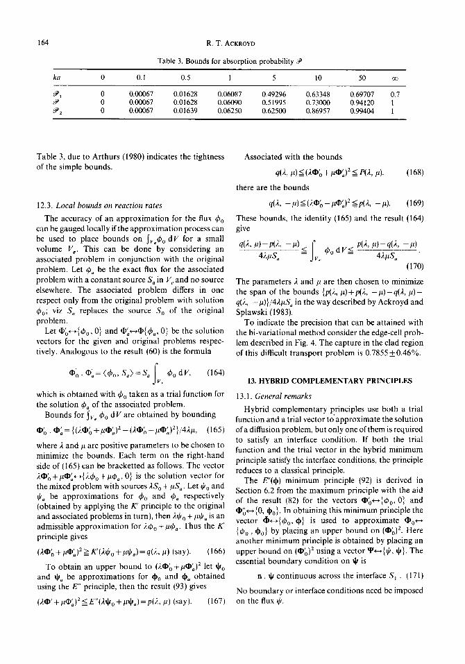
164 R. T. ACKROYD
Table 3. Bounds for absorption probability y.,~
ka 0 0.1 0.5 1 5 10 50 oc
~t 0 0.00067 0 . 0 1 6 2 8 0 . 0 6 0 8 7 0 . 4 9 2 9 6 0 . 6 3 3 4 8 0.69707 0.7 ?~ 0 0.00067 0 . 0 1 6 2 8 0 . 0 6 0 9 0 0 . 5 1 9 9 5 0 . 7 3 0 0 0 0.94120 1 ~2 0 0.00067 0 . 0 1 6 3 9 0 . 0 6 2 5 0 0 . 6 2 5 0 0 0 . 8 6 9 5 7 0.99404 1
Table 3, due to Arthurs (1980) indicates the tightness of the simple bounds.
12.3, Local bounds on reaction rates
The accuracy of an approximation for the flux q5 o can be gauged locally if the approximation process can be used to place bounds on ~vo~bo d V for a small volume V e. This can be done by considering an associated problem in conjunction with the original problem, Let q~, be the exact flux for the associated problem with a constant source S a in V e and no source elsewhere. The associated problem differs in one respect only from the original problem with solution qSo; viz S a replaces the source S o of the original problem.
Let q~o,---,{~bo, 0} and qb'~--~q){q~ , 0} be the solution vectors for the given and original problems respec- tively. Analogous to the result (60) is the formula
0 o . ,I , ;=<~o, S a ) = S , f v° qSO dV, (164)
which is obtained with q~o taken as a trial function for the solution ~b, of the associated problem.
Bounds for ~v. q~o dV are obtained by bounding
0 ' o . O '={(20 'o +l~O'.)2-(20'o-l tO')z}/421~, (165}
where ;t and/~ are positive parameters to be chosen to minimize the bounds. Each term on the right-hand side of (165) can be bracketted as follows. The vector 20 o +/~O;~{2q~ o + ~q~,, 0} is the solution vector for the mixed problem with sources 2S o + #S.. Let Oo and 0, be approximations for ~b o and 4~. respectively (obtained by applying the K' principle to the original and associated problems in turn), then 2~b o + #0. is an admissible approximation for 2q~ o +/~b a. Thus the K' principle gives
(,,~,O'o +ll¢|)'a)Z~K~(/tl/Io+121/l a)=q(,1., ll) (say). (166)
To obtain an upper bound to (20o +/~O'.) 2 let qo and q , be approximations for doo and d0, obtained using the E" principle, then the result (93) gives
(20'+~' ,)2<=E"(2~IIo+~a)=P( 2'- U) (say). (167)
Associated with the bounds
q(2,/0 <(20o + #O',)2 < P(2,/~). (168)
there are the bounds
q(2, - /0<(2Oo-~O ' , )2<p(2 , -/~). (169)
These bounds, the identity (165) and the result (164) give
q(2, U)- p(2,42/aS, - # ) = < fv~ 4)° dV_<_ p(2,/~)- q(2,42/~S, - # )
(170)
The parameters 2 and # are then chosen to minimize the span of the bounds {p(2, #)+p(2, - # ) - q ( 2 , ~ ) - q(2, -/~)}/421~S, in the way described by Ackroyd and Splawski (1983).
To indicate the precision that can be attained with the bi-variational method consider the edge-cell prob- lem described in Fig. 4. The capture in the clad region of this difficult transport problem is 0.7855_+ 0.46%.
13. HYBRID COMPLEMENTARY PRINCIPLES
13.1. General remarks
Hybrid complementary principles use both a trial function and a trial vector to approximate the solution of a diffusion problem, but only one of them is required to satisfy an interface condition. If both the trial function and the trial vector in the hybrid minimum principle satisfy the interface conditions, the principle reduces to a classical principle.
The E"(do) minimum principle (92) is derived in Section 6.2 from the maximum principle with the aid of the result (82) for the vectors Oo*--~{~b o, 0} and OC--'{0, doo}. In obtaining this minimum principle the vector ~-~{q~0, do} is used to approximate 00*-* {~bo, doo} by placing an upper bound on (00) 2. Here another minimum principle is obtained by placing an upper bound on (Oo) z using a vector ~g*-@p, ~}. The essential boundary condition on q is
n. ~ continuous across the interface S 1 . (171)
No boundary or interface conditions need be imposed on the flux qJ.
A least squares principle 165
Since this minimum principle employs an approxi- mation for the net current which is continuous everywhere, it is a natural principle to use with the nodal method. Henry (1975) observed that the essential idea of the nodal method is to relate the neutron currents across the interface of two zones, or nodes, to the average flux levels in those zones. This idea has been illustrated above on deriving a nodal method from a finite element method employing the E"(dp) principle, with ~b satisfying the same essential bound- ary condition as d/. A flux is associated with d~ by making d~ the gradient of the flux and imposing a neutron conservation on the elements or nodes. The resulting expression for the flux in an element is then an incomplete polynomial on the local co-ordinates of the element. For the hybrid minimum principle there is no such restriction on the expression for the flux qJ within an element.
A maximum principle complementary to the hybrid minimum principle is obtained in a similar way using a vector ®,--,{ 0, 0} to place a lower bound on (~o) 2. The essential boundary condition for ® is
0 continuous across the interface S~ . (172)
There is no need to impose any boundary or interface conditions on 0.
The hybrid principles are related to the K'(qS) and E"(~b) principles described previously. For example if the specific choice
~ = -DV~O (a)-[ (173) (
~0 =continuous across the interface S~ ( b ) J
is made, then the minimum principle
K ' (~ , )+ . fvE ~( -DV2~,+E~0-S) 2dV
+ f (~+ ~zDn" V~) 2 dS/~Z>(~o)2>K'(~) 3s 2
(174)
is obtained. This principle for diffusion theory is the analogue of a minimum principle for transport theory. Ackroyd (1981), which has been applied by Ackroyd and Splawski (1982) in the determination of local error bounds. The practical disadvantage of the minimum principle (174), viz the satisfaction of the continuity of both n. ~ and ~b across S~, does not arise with the hybrid minimum principle.
13.2. Hybrid minimum principle Let the trial vector ~ and its first derivatives be
continuous throughout the volumes V~ and V 2, satisfy
the condition (171) on S 1 the interface of V 1 and V 2, and be continuous on the bounding surface S 2. The trial function @ and its first derivatives are assumed to be continuous within Ii"1 and V 2, and on S 2. The minimum principle
K'(¢,t+ W(~,, ~)__>(~o) ~ (175)
then holds, with equality if, and only if, ff = ~b o and =d~o. Here
K'(q0 = (2qJ, S ) - ( ~ b , Z~) - (V f f . DV~b)
-- _IS2 ~lj2 dS/~2
W'(~, ~ ) = ( t + p ) ( E - ' ( d i v ~ + Y.~,- S),
div~ + EqJ- S)
+(D-'(~+DVqJ).(~+DV~)) (176)
fS r + 0 +2 n" q [ ~ ] r - o dS x
+ ~ (I,k- ~2n. ~1/) 2 dS/~t 2 ds 2
and p>0 . The parameter p can be set to zero, and then the
following results hold:
(a) If ~ and ff are independent, equality holds for the result (175) for any ff if, and only if, ~ =~o-
(b) If ~ and ~p are dependent in the following ways equality holds for the result (175)if, and only if,
= ~o and ~0 = 4% Case (i);
~b=Z ~(S- dive) (177)
within each region. Case (ii)
= - DVq,, i and i
( (178) f v (S -E t~)dV=- ;s n" DV~O dS. f
The principle (175) is derived below for a system with two regions V 1 and V 2 but the derivation can be generalized readily for a system of many regions to make it applicable to the finite element method.
The involvement of the functional K'(~9), in the hybrid principle (175) indicates a connection with the classical K' principle. The particular choice
~1/= dp o ~ (179) tp continuous across S~ )
is admissible in the hybrid principle. With d/=dpo the
166 R.T. ACKROYD
principle (175) and the diffusion equation (2) give for p = 0
~ ( ~ ) + <~ ' -~o , Z(~O- ¢o)>
+ <V(~O- ~bo) • DV(~-¢o)>
;, .o +2 n- ~bo[~O],_ o d S + (O-~bo) 2 dS/ct 2 1 2
= ((I)o) 2. (180)
Imposing the continuity of ~k gives
K'(0)_-< (Oo) 2 (181)
i.e. the maximum principle (65) is recovered.
13.3. Derivation of the hybrid minimum principle
Let T'*-*{~9, 0} and ~"*--,{0, 4} be approximations for ~o(¢o, 0) and ~o,--~{0, dpo } respectively. Initially no boundary conditions are imposed on ff and 4. Subsequently the boundary condition (171 ) is imposed to obtain a minimum principle for the approximation
• = ~ ' + ~ " (182)
for the exact solution vector ~o. When @ is discontinuous across S 1 the result
~(q,) + ~ {2[¢,n ,+o r+o 2 • ~bo]r_o-W([~#]~_o) } dS
ds 1 + ( V ' - ~ o ) 2 = (~0) 2 (183)
of appendix C holds• The vectors in equation (182) are related also by
(ltP - - ( l ) o ) 2 : ( V ' - - (]Do) 2 -'F ( V " - - (DO) 2
+ 2 f [qln" 0o + (¢o-~#)n" "vJd'qr+°r- odS ds 1
(184)
This is the result (B10) of Appendix B. Expressions are obtained below for ( ~ " - ~ o ) 2 and ( ~ - ~ o ) 2 so that (~, _ ~ ) 2 , (~,, _ (!)o)2 and (~ - ~o) 2 can be eliminated from equations (183) and (184).
An expression for ( ~ " - ~ o ) 2 is obtained using the scalar product (68) and the boundary condition (3), viz
( ~ - _ _ ~ ) 2 = <)-'~ - 'div(4 - ~bo), div( 4 - d#o)>
+ <D -l(4--dpo)" (4--dPo)>
+ f w'([n ,+o 2 " 4 ] r -o ) dS Js 1
+ ~ ct2(n • [4-(~o]) 2 dS. (185) .) s 2
Similarly with the aid of the differential equation (2) and the boundary conditions (3) and (4)
(~ - @o)2 = <X - 1 (div 4 + X¢, - S),div4 + X~O - S>
+ ( D - t ( 4 + DV$)" (O+ DVtp)>
fS r + O 2 Wt all-It + 012 ~" q- {W([-I//]r_O) + ([n" dS ~" J r - - 0 ! ) 1
+ r (~-~2n" ql) 2 dS/a2• (186) ds 2
The elimination gives
4)=(®o):+2 fs or. r+0 • 4 ] r 0 dS 1
+ I p<z l[div(¢-¢o)+Y-(~-~0o)], div(4-¢o)q
+ ~;(~' - 4 ' o i )
+ <Z- l d i v ( 4 - ~o), div(4 -~o)>
+ <D - I(4-d#o)'( 4-~o)>.
+ f ~ 2 ( n " [4--d~O]) 2 dS. Js 2
(187)
The minimum principle (175) arises from the result (187) on imposing the boundary condition (171). Equality holds in the minimum principle (175) for p>0, if, and only if, ~=d~o and 0 = ¢ 0 almost everywhere; because the bracketted terms of (187) are positive definite.
13.4. Derivation of a classical difference scheme
The hybrid minimum principle in conjunction with simple finite element representations for ~p and 4 gives a classical difference scheme for the diffusion equation when the parameter p is large. The finite element method in conjunction with the appropriate vari- ational principle thus embraces nine-point schemes for the flux, ten-point schemes for the currents, five-point nodal schemes for average fluxes and currents, and the classical five-point scheme for fluxes• All these schemes are based on the use of linear elements with an appropriate variational principle. The finite element method therefore provides not only a means of solving the diffusion equation over irregular meshes, but ways of setting up difference schemes of both the classical and nodal kinds for regular meshes.
For the element Vm., Fig. 10, of a homogeneous system put ~b= C.,. a constant. Define 4 for this element by
@= - - D x
i[(C,. + ,, . -Cm)(1 + ~)+ (C m - C,._t, .)(1 - ()]/2h +j[(Cm,. +, - Cm)(1 + ~/)+ (C,~ - Cm, ._,)(1 - r/)]/2kJ
(188)
A least squares principle 167
The normal components of k0 are -D(C , .+ , . . - C.,.)/h, -n (cm. -Cm_, . . ) /h , -D(C.,..+,-C,,,.~/k
n- ~, ), and -D(Cm-Cm, a)/k at the nodes (m+ ~ n ( m - ½, n), (m, n + ½) and (m, n - ½) respectively. Since n . O is continuous across interfaces, ~ and ~ are admissible in the hybrid minimum principle (175). The coefficients Cm. etc. are found by minimizing
2(~k, S ) - ( ~ , ~ k ) - ~ ¢2 dS/~2+(D -tdl. ~)" ds 2
fS r + O +2 n" ~[~/]r--O dS t
+ f (ip_ct2n. ~)2 dS/~2/(1 +p) 3s 2
+ (1 + p) + <E- '(divq + Y.$ - S), div~ + E$ - S>
For p large this gives
i.e. div~ + E f t - S= 0
__D~Cra+ I, . - 2C,.. + C._ , , . l h 2
C, . .+ L--2Cm.+ C.,,._ 1} + • k2
+ E C , . . - S = 0 (189)
a classical difference scheme. The excess of K'(~) + IV' (¢, ~) over (0'0) 2 is then (E - ld iv (~ -~o ) , d iv (~- ~bo) > + (D - t ( ~ - dpo ) " (~--dpo > +j's ~2(n • [~-- ~0]) 2 dS+ 2Ss,q~o[n r+0 • ~ ] , - o dS.
Since Cm. is the average flux in V,,. the difference scheme (189) is in effect a nodal scheme--the simplest.
13.5. Hybrid maximum principle
The maximum principle complementary to the minimum principle (175) is
E"(0)- ~4r'(0, 0) < (00) 2 (! 90)
where the functionals E"(0) and W"(0, 0) are defined by
E"(0) = <div0 - S, E- ' (d iv0- S)>
+ ( D - 1 0 " 0 ) + l" (n • 0 ) 2 ~ 2 dS, (191) js 2
and
W"(0, 0) = (1 + p)(div0 + E0 - S, E - l(div0 + E0 - S) )
+ <D(0 + DVO) • (0 + V0)>
+2fs 0In, ,+o 0],_ odS 1
F + / (O--~2n" 0)2 dS/a2' (192)
3s 2
with p > 0. However for the principle (190) to hold the essential
boundary condition
0 continuous across S, (193)
has to be satisfied• This boundary condition is complementary to the boundary condition (171) for the minimum principle (175).
13.6. Derivation of the hybrid maximum principle
Let O',---~{0, 0} be an approximation for 00+-* {q~o, 0} and take 0%-,{0, 0} as an approximation for Oo+--,{0, d~o}, then
O = O ' + O " (194)
is an approximation for Oo*--~{q~ o, ~bo}. These vectors are related by the result (B10) of Appendix B in the following way
( O - • o)2 = (O' - Oo)2 + (O" - Oo)2
+2 fsjOn *o+ + (#5 o --0)[n " Var--o~alr+Ot dS. (195)
There is also the functional relationship of Appen- dix D, viz
E"(0) + f {w'([n • 0]~_+°) 2 - 2 [ n . r+o q~o0], o} dS 3s 1
- ( O " - 0 0 ) 2 = (00) 2 (196)
involving ( 0 " - 0 0 ) 2 . Expressions are obtained now for ( 0 - 0 0 ) 2 and ( 0 ' - 0 0 ) 2 so that these quantities and (O"-Oo) 2 can be eliminated from equations (195) and (196).
On using the definition (68) of a scalar product with the specification (2)-(4) of the diffusion problem one obtains
( 0 - - (]Do) 2 = ( d i v O + EO - S, E - ~(divO + EO - S))
+ (D - ' (0+ DVO). (0+ DV0))
fS r + O 2 + {w(E0]r o) 1
+w' ( [n . 0]~+o°) z} dS
+ ~ ( 0 - a 2 n • 0) 2 d S / ~ 2, (197) 3s 2
168 R.T. ACKROYD
and
( 0 ' - o o ) 2
= <0-- (9o, E(0-- (9o)) + <V(0- (9o) - DV(0- (9o))
+ w([0]r_o) d S + (0--(9o) 2 dS/ot 2. 1 2
(198)
Eliminating ( O - ~o) 2, ( O " - ~ o ) 2 and ( O ' - ~ o ) 2 from the equations (195)-(198) gives, on invoking the diffusion equation for (9o,
E"(0)- W"(0, 0)+2 r [On. "to J , -0 ~ q,+0 d S + 3s 1
( 0 - (90, Z ( 0 - (9o)) + ( V ( 0 - (9o)" DV(O-- ( 9 o ) )
{.
+ JSz ( 0 - (90) 2 dS/o: 2
+ p(div(O - doo) + Z ( 0 - (9o),
Z - ' [d iv (0- doo) + Z ( 0 - (90)])
=(~o) 2. (199)
Since the bracketed term of equation (199) is positive definite and the boundary condition (193) holds, the maximum principle
E ' (O)- W"(0, O) =< (@0) 2 (200)
is established. With p>O equality holds in the principle (200) if, and only if,
0 = ( 9 0 almost everywhere. (201)
0 = d o o
The result (199) can be used also to recover the minimum principle (93), because putting
p=O 0=(90 (202) n • 0 continuous across interfaces
in the expression (199) gives
E"(0)=(@~,)2 + W"((9 o, 0)
= (~o) 2 + <div(0- doo)" E ' d iv (0 - doo))
+ <D - '(O--doo) " ( 0 - doo))
+ f ((9o - ~ 2 n ' 0) 2 dS/o~ 2 ,/s 2
i.e. E"(0) > (~o) 2. (203)
13.7. Hybrid principles permit the use of complete elements
Hybrid principles permit the use of complete elements. For example the K'(~)+ W'(q,, q) minimum principle permits the use of complete elements for the flux ~p, because q, does not have to satisfy any interface or boundary conditions. Here the type of elements used by the classical K'((9) principle, the K"(do) or E"(do) principle, and the hybrid K'(~0) + W'(qJ, ~) principle are compared.
13.7.1. K'((9) maximum principle. This principle is restricted to conforming elements for the flux approxi- mation (9. The bi-linear element specified by the formula (125) satisfies the continuity condition for (9 on the sides, but it is not complete because there are no terms in 4 2 and r/2 in the expression for (9.
13.7.2. E"(do) minimum principle. The element for the net current d o used by the K"(do) or E"(do) principles must satisfy the condition that n. do is continuous across the sides. For example the expression (135) for the net current meets this requirement. Associated with this expression for the net current there is the expression (138) for the flux. The flux is not continuous on the sides of the element because of the presence of (z and r/2 terms and the absence of a 4t/term.
13.7.3. K'(~b) + W'(~,, q) minimum principle. To illus- trate the use of complete elements for the flux consider the determination of @ for a system with a rectangular mesh. The procedure can be applied however to an arbitrary mesh. Suppose the net current approxima- tion ~ has been determined using an expression of the kind (135), viz
~/= i[a~. +_L, + a" _ ½,, + (a" + ~.. - a~,_ ½, n)4]/2
+jEak, . +½+ak.._½+ (a" .+½--a" ._½)t/]/2. (204)
The coefficients a~,, +½., etc. are presumed to have been found by solving the equations of the kinds (136) and (137) directly, as this would be the procedure for an arbitrary mesh.
With ~ determined the flux O' associated with the E"(~) principle can be obtained using an expression of the kind (138), viz
- h r~a' , ~ -a ' , ]Y q / = ¢ (o , o) ~ - ~, m : . . - - ,,+~ . . . .
+ (a'm+½. n --a',._½..)C/2]
- k m,. + :)~ 4D [(a~,,. ~ + a' '
+ (a~.,. + ~ - a ; . , . _ 0,12/2]. I205)
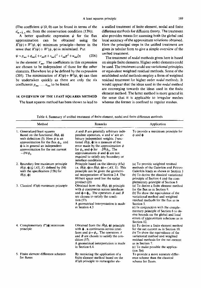
A least squares principle 169
(The coefficient ~b'(0, 0) can be found in terms of the a~+½., etc. from the conservation condit ion (139)).
A better quadratic expression ~b for the flux approximation can be obtained using the K ' (~ )+ W'(ff, ~) minimum principle--bet ter in the sense that K'(~b)+ W'(~,, ~) is minimized. Put
~b = Pro, + qm,~ + rmnrl +smn¢ 2 + tranrl 2 + Urnn~tl (206)
in the element Vmn. The coefficients in this expression are chosen to be independent of those for the other elements. Elsewhere let ~b be defined by the expression (205). The minimization of K'(~,) + W'(~b, d~) can then be undertaken quickly as there are only the six coefficients p ~ . . . amn to be found.
14. OVERVIEW OF THE LEAST SQUARES METHOD
The least squares method has been shown to lead to
a unified treatment of finite element, nodal and finite difference methods for diffusion theory. The treatment also provides means for assessing both the global and local accuracy of the approximate solutions obtained. Here the principal steps in the unified treatment are given in tabular form to give a simple overview of the unified treatment.
The treatment of nodal methods given here is based on simple finite elements. Higher order elements could be used. The treatment could use variational principles or equivalent weighted residual methods. Some of the established nodal methods employ a form of weighted residual treatment for higher order nodal methods. It would appear that the ideas used in the nodal method are converging towards the ideas used in the finite element method. The latter method is more general in the sense that it is applicable to irregular meshes whereas the former is confined to regular meshes.
Table 4. Summary of unified treatment of finite element, nodal and finite difference methods
Method Remarks Application
1. Generalized least squares Based on the functional/t(~b, tk) with definition (5). Here ~b is an approximation for the flux ~b o, and
is in general an independent approximation for the net current -DV~b 0
2. Boundary free maximum principle /~(~b, d~)< (AS, S) defined by (16) with the specification (15b) for /~(~, ,~)
3. Classical K'(~b) maximum principle
4. Complementary E"(dp) minimum principle
5. Finite element difference schemes for fluxes
A and B are generally arbitrary inde- pendent operators, w and w' are ar- bitrary independent weights. Func- tional/t(~, dp) is a measure of the error made by the approximation ~b for ~b o and ~p for -DV~b 0. The approximations ~b and $ are not required to satisfy any boundary or interface conditions Principle based on the identity (15a) i.e. ~(~b, d#)+/t(~b, ~)= (AS, S). This principle can be given the geometri- cal interpretation of Section 2.4. The Hilbert space used has the scalar product (21) Obtained from the H(~b, $) principle with ~b continuous across interfaces and $=$0 . The operators A and B are chosen to satisfy the condi- tion (57). A geometrical interpretation is made in Section 4.3
Obtained from the/t(~, ~p) principle with d~. a continuous across inter- faces and q~ = ~b 0. The operators A and B are chosen to satisfy the con- dition (57). A geometrical interpretation is made in Section 6.4.
By restricting the application of a finite element method based on the K'(~b) principle to rectangular ele-
To provide a maximum principle for ~b and d~
(a) To provide weighted residual methods of the Galerkin and Petrov- Galerkin kinds as shown in Section 3 (b) To derive the classical variational principle of Section 4 and the com- plementary principle of Section 6 (a) To derive a finite element method for the flux as in Section 9. (b) To show the equivalence of the variational method and weighted residual methods for the flux as in Section 5. (c) In conjunction with the comple- mentary principle of Section 6 to de- rive bounds on the global and local errors of approximate solutions as in Section 12. (a) To derive a finite element method for the net current as in Section 10. (b) To show the equivalence of the variational method and weighted residual methods for the net current as in Section 7. (c) To make possible the applica- tion 3(e). To provide a more accurate differ- ence scheme than the classical scheme for fluxes.
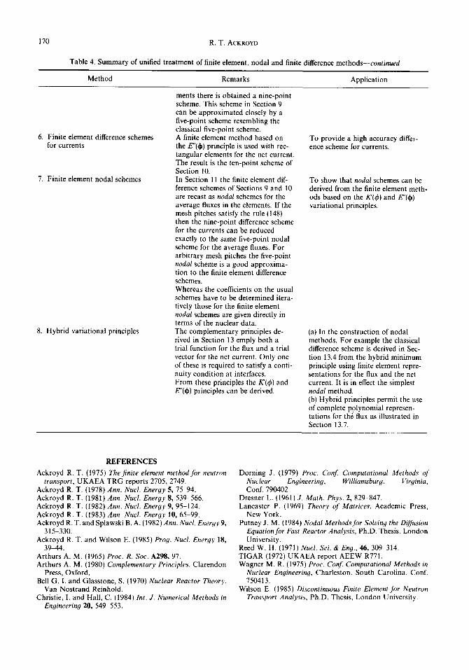
170 R. T. ACKROYD
Table 4. Summary of unified treatment of finite element, nodal and finite difference methods--continued
Method Remarks Application
6. Finite element difference schemes for currents
7. Finite element nodal schemes
8. Hybrid variational principles
ments there is obtained a nine-point scheme. This scheme in Section 9 can be approximated closely by a five-point scheme resembling the classical five-point scheme. A finite element method based on the E"(~) principle is used with rec- tangular elements for the net current. The result is the ten-point scheme of Section 10. In Section 11 the finite element dif- ference schemes of Sections 9 and 10 are recast as nodal schemes for the average fluxes in the elements. If the mesh pitches satisfy the rule (148) then the nine-point difference scheme for the currents can be reduced exactly to the same five-point nodal scheme for the average fluxes. For arbitrary mesh pitches the five-point nodal scheme is a good approxima- tion to the finite element difference schemes. Whereas the coefficients on the usual schemes have to be determined itera- tively those for the finite element nodal schemes are given directly in terms of the nuclear data. The complementary principles de- rived in Section 13 emply both a trial function for the flux and a trial vector for the net current. Only one of these is required to satisfy a conti- nuity condition at interfaces. From these principles the K'(~) and E"(~) principles can be derived.
To provide a high accuracy differ- ence scheme for currents.
To show that nodal schemes can be derived from the finite element meth- ods based on the K'(q~) and E"(~) variational principles.
(a) In the construction of nodal methods. For example the classical difference scheme is derived in Sec- tion 13.4 from the hybrid minimum principle using finite element repre- sentations for the flux and the net current. It is in effect the simplest nodal method. (b) Hybrid principles permit the use of complete polynomial represen- tations for th6 flux as illustrated in Section 13.7.
REFERENCES
Ackroyd R. T. (1975) The finite element method for neutron transport, UKAEA TRG reports 2705, 2749.
Ackroyd R. T. (1978) Ann. Nucl. Energy 5, 75 94. Ackroyd R. T. (1981) Ann. Nucl. Eneryy 8, 539-566. Ackroyd R. T. (1982) Ann. Nucl. Energy 9, 95-124. Ackroyd R. T. (1983) Ann. Nucl. Energy 10, 65 99. Ackroyd R. T. and Splawski B. A. (1982) Ann. Nucl. Energy 9,
315 330. Ackroyd R. T. and Wilson E. (1985) Prog. Nucl. Energy 18,
39~4. Arthurs A. M. (1965) Proc. R. Soc. A298, 97. Arthurs A. M. (1980) Complementary Principles. Clarendon
Press, Oxford. Bell G. I. and Glasstone, S. (1970) Nuclear Reactor Theory.
Van Nostrand Reinhold. Christie, I. and Hall, C. (1984) Int. J. Numerical Methods in
Engineering 20, 549 553.
Dorning J. (1979) Proc. Conf. Computational Methods of Nuclear Engineering, Williamsburg, Virginia, Conf. 790402.
Dresner L. (1961) J. Math. Phys. 2, 829~847. Lancaster P. (1969) Theory of Matrices. Academic Press,
New York. Putney J. M. (1984) Nodal Methods for Solving the Diffusion
Equation for Fast Reactor Analysis, Ph.D. Thesis, London University.
Reed W. H. (1971) Nucl. Sci. & Eng., 46, 309 314. TIGAR (1972) UKAEA report AEEW R771. Wagner M. R. (1975) Proc. Conf. Computational Methods in
Nuclear Engineerino, Charleston. South Carolina, Conf. 750413.
Wilson E. (1985) Discontinuous Finite Element Jbr Neutron Transport Analysis, Ph.D. Thesis, London University.
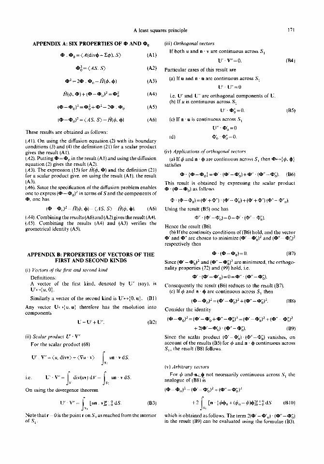
A least squares principle 171
A P P E N D I X A: SIX PROPERTIES OF • A N D • o
O . • o = (A (divdo + gq~ ), S) (A1)
020 = (AS , S ) (A2)
O 2 = 2 0 . • o -/4(~b, do) (A3)
f l (~, o ) + ( o - • 0)2 = o g (A4)
( 0 - 0 0 ) 2 = 0 o 2 + 0 2 - 2 0 . • o (A5)
(O - Oo) 2 = (A S, S) -/~(~b, do) (A6)
These results are obtained as follows:
(A1). On using the diffusion equation (2) with its boundary conditions (3) and (4) the definition (21) for a scalar product gives the result (A1). (A2). Putting • = • o in the result (A l) and using the diffusion equation (2) gives the result (A2). (A3). The expression (15) for/4'(q~, O) and the definition (21) for a scalar product give, on using the result {A1), the result (A3). (A6). Since the specification of the diffusion problem enables one to express ( O - Oo) 2 in terms of S and the components of O, one has
( O - O o ) 2 =/}(~b, do)=(AS, S ) - I:l(~p, do). (A6)
(A4). Combining the results (A6) and (A2) gives the result (A4). (A5). Combining the results (A4) and (A3) verifies the geometrical identity (A5).
APPENDIX B: P R O P E R T I E S OF VECTORS O F THE FIRST AND S E C O N D KINDS
(i) Vectors q[the first and second kind
Definitions: A vector of the first kind, denoted by U" {say), is u ' ~ { . , o}.
Similarly a vector of the second kind is U'~--,{0, u}. (BI)
Any vector U~--~{u, u} therefore has the resolution into components
U = U ' + U " . (B2)
(ii) Scalar product U' . V"
For the scalar product (68)
U ' . V"= (u, divv} + (Vu • v) - f un - vdS. j s 2
i e
On using the divergence theorem
U" V" = [ " [un. v][~ ° dS. (B3) J s i
Note that r - 0 is the point r on S~ as reached from the interior o f S 1 .
(iii) Orthooonal vectors
If both u and n • v are continuous across S t
U " V" =0 . (B4)
Particular cases of this result are
(a) If u and n- u are continuous across S t
U ' . U " = 0
i.e. U' and U" are orthogonal components of U. (b) If u is continuous across S 1
U ' - • o =0. (B5)
(c) If n • u is continuous across $1
u " . O o = 0
(d) 0 o . 0 o =0.
(iv) Applications o[ orthooonal vectors
(a) If ~b and n . do are continuous across S 1 then O*--}{ ~b, do} satisfies
O . { O - O o } = O ' - ( O ' - O o ) + O " . (O"-Oo) . (B6)
This result is obtained by expressing the scalar product • - ( O - 0 o ) as follows
O. ( O - Oo) = (O' + O"). (O' -,1%) + (O' + 0 9 (O" - O"o).
Using the result (B5) one has
a)" • ( o ' - ¢ o ) = o = o ' • ( o " - Oo).
Hence the result (B6). (b) If the continuity conditions of(B6) hold, and the vector
O' and 0 " are chosen to minimize ( 0 ' - O o ) z and ( 0 " - O o ) 2 respectively then
0 . ( 0 - 0 0 ) = 0 . (B7)
Since ( 0 ' - 0 o ) 2 and ( 0 " - O o ) 2 are minimized, the orthogo- nality properties (72) and (99) hold, i.e.
o , . (o ,_O,o)= 0 = o, , . (o, ,_ o0).
Consequently the result (B6) reduces to the result (B7). (c) If 4~ and n . do are continuous across S 1 then
( 0 - 00) z = ( ' P ' - 00) 2 + ( 0 " - 0 0 ) 2. (B8)
Consider the identity
(O - (Do) z = (0 ' - O o + O" - Oo) z = (O' - 00) 2 + (O" - Oo) ~
+ 2(O' - Og). (O" - Oo). (B9)
Since the scalar product ((l)'-(l)o)-(O"-(I)o) vanishes, on account of the results (B5) for q~ and n . do continuous across S~, the result (B8) follows.
(v) Arbitrary vectors
For ~b andm.z~, not necessarily continuous across S l the analogue of (B8) is
( O - - 1110)2 = (1~ ' {l[}O )2 + 11~1" - - {~O) 2
~,S n " I + r + O +2 [ ,~doo (4 'o-4 ')do],_odS (B10) i
which is obtained as follows. The term 2 ( 0 ' - 0 ' o ) - ( 0 " - O o ) in the result (B9) can be evaluated using the formulae (B3).
172 R.T. ACKROYD
Since 4>o n. #o is continuous across S 1
(~'-(]Do)" (0"-¢1)' ~) = ~ [n" {4>¢o+(4>o-¢)¢}]~+_o ° dS j s i
Hence the result (B10) is obtained.
A P P E N D I X C: THE FUNCTIONAL RELATIONSHIP
K'(¢) + f {2[¢n. dpo],r+°_ o - w([¢]~-+ o°)2} dS j s 1
+ ( v ' - o ~ ) 2 = (cpo)2,
where K'(¢) and F(¢, ¢) are given for arbitrary ¢ by the definitions (63) and (60), viz
K'(¢)= 2(¢, S) -F(¢ , ¢)
F ( ¢ , ¢ ) = ( ¢ , E ¢ ) + ( V ¢ . D V ¢ ) + f ¢2dS/~2. 3s 2
Consider the identity
(®o)2 = ( v ' - ® o ) ~ + 2 v ' . ~ o - ( V ' ) 2 ( e l )
for ~ o ~ { 4 > o , 0} and '1",- ,{¢, 0} with n o boundary condi- tions imposed on ¢. The definition (68) of a scalar product gives, on using the boundary conditions for 4>0,
~P" @~ = (¢, E4>o) + (V¢" DV4>o) + f ¢4>o dS/0:2. JS 2
This result can be written as
'|" " O'o=<¢, s> - fv div(¢,t,o) dV + fs ¢4>o dS/:~
with the aid of the diffusion equation (2)• Using the boundary conditions (4) with the divergence theorem gives
utv'cYP°=(¢'S>+ f r + ° d S [ ¢ n - O o ] r - o (C2) 3s~
The above definition of K'(¢) and the result (C2) give
fs [¢U.¢o],_ d S - F ( ¢ , ¢ ) (C3) K ' ( ¢ ) = 2 V ' . ~ - 2 "+ o o l
The definitions (60) and (68) give
fS r+0 2 (I][/,)2 = F ( ¢ , ¢) + W([¢]r_0) dS. (C4) 1
Substituting the results C3 and C4 in the identity (C1) gives the required relation
((]Do)2=(~1~'-(~)~))2.+ ~ {2[~0n. ~+o ,+o 2 ~o],_o-W([~b],_o) } dS 3s 1
+ic (¢ ) . (c5)
A P P E N D I X D : THE FUNCTIONAL RELATIONSHIP
E"(0) + fs{W,([n. 0]~+o)2_2[ n . 4>O0]r_0 }r+0 dS
- t0" - ¢0) 2 = (00 ) 2,
where E"(0) is defined for arbitrary 0 by equation 02) as
E"(0) = (E - a (div0- S), div0 - S) + (D 10. O)
+ fs2 (n. 0)2~ 2 dS.
Consider the evaluation of the last two terms in the identity
((I~o)2 = (O"-- {]Do)2 + 20" • (l}o - (O") 2 (D1)
for ~o ' - '{0, ¢o} and e"*-,{0, 0}, with no boundary condi- tions imposed on 0. The definition (68) of a scalar product gives, on using the boundary conditions for ~o,
0 " ' ®o = (div0, Z- ldiv~o) - (0" V4> o) + f 4>o n. 0 dS. 3s 2
Using the diffusion equation (2)
O"" ~'~) = (div0, E- 'S) - fv div{4>°0} d V
+ is2 4>°n" 0 dS,
which gives with the aid of the divergence theorem and the boundary condition (4)
O,,.Oo=<divO, X-,s>+ f s [4>o n . r+o 0]r_ o dS. (D2) 1
The definition (68) of a scalar product gives
(0") 2 = (X- idly0, div0) + (D - tO. 0)
+ ~ w'([n ,+o 2 dS • 0Jr_0 ) j s 1
+ f o~2(n - 0) 2 dS. (D3) j s 2
Using the results (D2) and (D3) with the functional relation- ship
(CDo) 2 +(*o) 2 = ~ = (S, E-aS), (D4)
the identity (D1) becomes
fS 0Jr_0) --214>on 0It_O} dS E"(0)+ {w'([n. ,+o 2 . ,+o 1
- (0" - (!)o) 2 = ((l)o) 2. (D5)