Embed Size (px)
Citation preview

NASA Technical Memorandum 102385
ICOMP-89-28
A Least-Squares Finite Element Method forIncompressible Navier-Stokes Problems
Bo-nan Jiang
Institute for Computational Mechanics in PropulsionLewis Research Center
Cleveland, Ohio
October 1989
12A
(*lASIA-IM-102315) A L_:A_T -SOUARES IzTIilTF
ELEMENT M_THOr) FOR INCOMPRESST_LL
NAVIER-_TnK_S pRuBLEMS (NASA) Z2 pCSCL
Nq0-12231
Unclas
G31_4 0239277
LY _
https://ntrs.nasa.gov/search.jsp?R=19900002915 2020-03-20T09:41:41+00:00Z


A LEAST-SQUARES FINITE ELEMENT METHOD
FOR INCOMPRESSIBLE NAVIER-STOKES PROBLEMS
Bo-nan Jiang*
Institute for Computational Mechanics in Propulsion
Lewis Research Center
Cleveland, Ohio 44135
SUMMARY
A least-squares finite element method, based on the velocity-pressure-vorticity for-
mulation, is developed for solving steady incompressible Navier-Stokes problems. This
method leads to a minimization problem rather than to a saddle-point problem by the clas-
sic mixed method, and can thus accommodate equal-order interpolations. This method
has no parameter to tune. The associated algebraic system is symmetric, and positive
definite. Numerical results for the cavity flow at Reynolds number up to 10,000 and the
backward-facing step flow at Reynolds number up to 900 are presented.
1. INTRODUCTION
During the past decades various finite element methods for incompressible viscous flows
have been developed. Extensive results can be found in the literature. 1-6 Most of these
finite element methods are based on the velocity-pressure formulation because of its sim-
pler boundary conditions and easier extension to three-dimensions. Three methods are
commonly used to solve the velocity-pressure equations. They are the Galerkin mixed
method, the penalty method and the segregated method.
In the Galerkin mixed method, different elements have to be used to interpolate
the velocity and the pressure in order to satisfy the Ladyzhenskaya-Babu_ka-Brezzi(LBB)
condition for the existence of the solution. 7's Although for two-dimensional problems quite
a few convergent pairs of velocity and pressure elements have been developed, most of
these combinations employ basis functions that are not convenient to implement. For
three dimensional problems, this difficulty becomes more severe and only rather elaborate
constructions can pass the LBB test. Another difficulty is that the matrix associated with
the system of linear equations is both non-symmetric due to the convection terms in the
Navier-Stokes equations and non-positive-definite owing to the uncoupled nature of the
incompressibility constraint. Therefore, direct Gaussian elimination rather than iterative
techniques has been considered the only viable method for solving the system. But, for
three-dimensional problems, the computer resources required by a direct method become
prohibitively large.
*Work funded by Space Act Agreement C99066G.

ORIGINAL PAGE iS
OF POOR QUALITY
In the penalty method, the pressure is pre-eliminated by penalizing the continuity
equation. Involving only velocities, a considerable saving in computing time and computer
memory is achieved. However, in many engineering applications, the pressure may be the
most important design parameter, but the pressure recovered by using the perturbed con-
servation of m&qs equation exhibits oscillations due to the ill-conditioned pressure matrix.
Another disadvantage is the penalty parameter, whichfor small values causes loss of accu-
racy and for too large values sometimes prevents convergence to the solution. Furthermore,
because of the ill-condition due to the smallness of the parameter, the linear system can
not be solved by iterative techniques. Thus one can not use the penalty method to solve
large-scale problems.
The segregated method _'1°'il adopts a well-known SIMPLE-type finite difference al-
gorithm. Since the computation of velocity and pressure are decoupled by iteration, signifi-
cant computational efficiency can be achieved in computer storage and time. However, due
to the lack of correct pressure boundary conditions for the pressure correction equation,
the computed pressure maybe inaccurate. A comparative study of the segregated method
vs the Galerkin mixed method can be found in Reference 12.
In order to overcome these difficulties, we have been developing a least-squares finite
element method(LSFEM) 13'14'15 based on the first-order velocity-pressure-vorticity for-
mulation. Any good solver of Navier-Stokes equations should at least be able to solve the
Stokes equations. For the Stokes equations, this method leads to a minimization problem
rather than to a saddle-point problem, and the choice of combination of elements is thus
not subject to the LBB condition. The numerical experiments exhibit the optimal rate of
convergence for all variables with equal-order interpolations. A theoretical error analysis
supports this observation, is Furthermore, there are neither added parameters nor artifi-
cial dissipation nor upwinding. The resulting matrix is symmetric and positive definite.
Therefore, simple iterative techniques can be employed to solve large-scale problems on
vector and parallel computers.
In this paper, we describe the LSFEM which has all the above mentioned advantages
for solving the incompressible Navier-Stokes problems. The numerical procedure used in
the present study is based on a general framework of the LSFEM for systems of first-
order partial differential equations. 1_ For the sake of completeness, we disscus the LSFEM
for first-order systems in Section 2. Section 3 provides a derivation of the first-order
velocity-pressure-vorticity formulation for the Navier-Stokes equations. In Section 4 the
performance of the LSFEM is illustrated by the computational results for high Reynolds

number cavity flows and backward-facing step flows. Conclusions are given in Section 5.
2. LSFEM FOR FIRST-ORDER SYSTEMS
The LSFEM of interest here is based on minimizing the residual in differential equa-
tions in L 2 norm. The LSFEM requires that the trial functions be smooth enough to lie
in the domain of the differential operator. For example, for second-order differential equa-
tions, the LSFEM must use C 1 elements(plate or shell elements) which are not convenient
from the computational point of view. In order to use simple C o elements, we transform
the original differential equations into an equivalent system of first-order differential equa-
tions by introducing auxiliary unknowns. This can be realized for almost any governing
equation in mathematical physics.
We consider the boundary-value problem:
Lu_= f in fl (1)
B__: g on r (2)
where L is a first-order partial differential operator:
na at*
= + (3)i=i
fl C _,td is a bounded domain with a piecewise smooth boundary r, nd= 2 or 3 represents
the number of space dimensions, u_r = (ul, u2, ...ur,.,) is a vector of m unknown functions of
x__,Ai and A are m × m matrices which depend on x__,f is a given vector-valued function, B
is a boundary operator, and g is a given vector-valued function on the boundary. Without
loss of generality we assume that g_ is a zero vector.
Here, we do not discuss the existence and uniqueness of the solution to (1), because
these depend on the structure and properties of L and B, and the vector f. In the following
discussion, it is assumed that the problem (1) has a unique solution. We indicate that if
there is a solution to (1), then the following least-squares method produces an approximatesolution.
Throughout this paper, L 2 (fl) denotes the space of square-integrable functions defined
on fl with inner product
(u, v) =/_ uvdn u, v _ L2(n) (4)
3

and norm
llullo_-We define the Sobolev space as:
. _ L:(n) (s)
H'(n)-{_CL2(n);a_e L=(n),Vlal_<1} (6)
where a -- (r#l, a2, ..., and) E _qnd and ]a[ = a I -}- a 2 -Jr- ... nt- and , and define their associated
norms by
I1"11_- _ Ila%ll_ (7)
lal_<l
For the vector-valued function u_ with m components, we have the product spaces
L_(n)= (L_(n))_" (8)
_H'(n)= (H'(n))" (9)
and the corresponding normF_
• II_-IIg= _ II,,jllo= (lO)y=l
m
I1_-I1_= _ II"Jll,= (11)i=1
Considering the boundary condition of the boundary-value problem, we also define
the function space
_S= {u_ E (H'(II))m;Bu_ -- 0 on r} (12)
Let us suppose that f E L 2 and L : _S --. __L2. For an arbitrary trial function u_ E S, we
define the residual function R__= L_u - L" The LSFEM is based on minimizing the residual
function in a least-squares sense.
We construct the least-squares functional
z(_)= II1,_- ZIIo== (L_- ,#',_- ,f) (13)
Taking variation of I with respect to u_, and setting 61 = 0 and 6u_ = w__, lead to the
least-squares weak statement: Find u_E S such that
("_-,"_-)= ("_-,D vwc s (14)
4

In the approximate analysis, we first discretize the domain as a union of finite elements
and then introduce an appropriate finite element basis. Let ATedenote the number of nodes
for one element and _bi denote the element shape functions. If equal-order interpolations
are employed, that is, for all unknown variables the same finite element is used, we can
write the expansion
N. U2
u y
(15)
where (ul,u2,...,um)j are the nodal values at the jth node, and h denotes the mesh
parameter.
Introducing the finite element approximation defined in (15) into the weak statement
(14), we have the linear algebraic equations
KU---- F (16)
where the U is the global vector of nodal values. The global matrix K is assembled from
the element matrices
Ke =/_ (L_)I,L_2,...,L_Ne)T (L_I,L_2, ...,L_Ne)dfi¢
(17)
in which fie C fi is the domain of the eth element, T denotes the transpose, and the vector
F is assembled from the element vectors
Fe = /f_ (L_I,L_2,...,L_N°)T f dfi(18)
in which
L_j = _j,zA1 + j,vA2 + j,.As + g,jA (19)
REMARK 1 If L is an elliptic operator, then we have the inequality
(Lw__,Lu_) < MoIl_lllllu_l[1, (Lu_,Lu_) > o4[u_H2 (20)
for arbitrary u_,w__E S, where M0 and c_ are positive constants. That is, the bilinear form
(Lw, Lu__)is continuous and coercive. Following the classic argument(see,e.g., Reference 18,
p.26-28), if the exact solution is smooth enough, we can easily obtain the error estimate
II lll= I1 - hlll MoC hk (21)_X

where the constant C is independent of the mesh size h, and k denotes the order of complete
polynomial of shape functions. Furthermore, the L 2 error estimate can be obtained by the
Aubin-Nitsche trick(see, e.g., Reference 19, p.88). These facts indicate that all variables
with equal-order interpolations converge at the optimal rate.
REMARK 2. The matrix K is symmetric and positive definite. Therefore, iterative
techniques, such as the preconditioned element-by-element conjugate gradient method, 2°'21
can be employed to solve the resulting algebraic equations. This property means that large-
scale problems can be effectively solved on vector and parallel computers.
REMARK 3. The computational labor of iterative methods depends on the condition
number of the matrix K. If a second-order elliptic problem is solved numerically using the
classic Galerkin method on a uniform finite element mesh of size h, the resulting matrix
has condition number O(h-2). If the same problem is recast as a first-order system, and
then treated by the LSFEM, the condition number of matrix K remains as O(h-2). 22'23
That is, the LSFEM described here does not degrade the condition number.
REMARK 4. It is important to point out that there is no weighting parameter in our
LSFEM. Each equation in the first-order system is equally treated. That is, the LSFEM
is robust (with no parameter to tune ). People thought that in least-squares methods
one could put a large weighting factor on one equation in the system to emphasize the
importance of this equation over others. 24 Numerical experiments and theoretical analysis
show that this idea is incorrect. The weighting can not change the minimum point(zero)
of the least-squares functional, and thus can not change the solution except the condition
number of the resulting matrix. 2s Usually, the governing equations are nondimensionalized
by using the reference quantities of the problem. The nondimensionalization or scaling is
equivalent to weighting the residuals in the least-squares functional. By the same argument,
the scaling with different choice of the reference quantities will not change the LSFEM
solution.
REMARK 5 The formulation of LSFEM is simple and systematic. Once a LSFEM based
on a first-order system is coded, adaptation of the program to other problems is simply
carried out by modifying the subroutines associated with the coefficient matrices AI, A2,
A3 and A and the vector function f. In this way, one may develop a general-purpose
program.
3. VELOCITY-PRESSURE-VORTICITY FORMULATION
Consider the incompressible Navier-Stokes problem: Find the velocity u_ = (ul, u2, u3)
and the pressure p such that
V.u=O in 12 (22a)

1
u_. Vu__- _ Au_ + Vp- f__ in n (22b)
Here all wriables are nondimensionalized, f = (fz, fv) is the body force, and Re denotes
the Reynolds number, defined asUL
Re = mu
where L a reference length, U a reference velocity and u the kinematic viscosity. Of
course, the boundary conditions should be supplemented to complete the definition of the
boundary value problem.
Since the momentum equations(22b) involve second-order derivatives of velocity, the
direct application of least-squares method requires the use of inconvenient C 1 elements and
produces matrices with large condition number. 22 In order to use the LSFEM described
in Section 2, we must consider the governing equations of incompressible flows in the
form of first-order systems. There are several ways to do this. For example, one may
write the Navier-Stokes equations in velocity-pressure-stress formulation, which is useful
for viscoelasticity and non-Newtonian flow problems, but this formulation has too many
variables. Instead, we introduce the vorticity __ = V x u, and rewrite the incompressible
Navier-Stokes equations in the following first-order quasi-linear velocity-pressure_vorticity
formulation:
V.u=0
---1V _u . Vu__+ Re x o_ + Vp = f in fl (23)
_-Vxu_=0
We shall consider the two-dimensional problem only:
au av
=0
au au _p 1 ao_ = ?z+
Ov Ov Op 1 Ow
u -_-_x+ v -_-_y+ ay Re Oz = /v
au avw+ -0
ay az
in n (24)
We can write(24) in the general form of a first-order system(I), in which
( oo (ilOO)0 1 0 0 0Ax = u 0 1 A2 =--R--_ v 1 0
--1 0 0 0 0 0
7

A= f= u= (25)0 0 0 - - p
0 0 0
Since the system is of first-order, the boundary conditions are thus very simple, and
do not involve the derivatives of unknowns. Let (FI, F2, Fs, F4, Fs) denote the sides of F.
The unit outward normal vector to F is denoted by _n, and the tangential vector to F by t.
We may consider, for instance, the following boundary conditions:
(a) u=0,v=0on the F1 (the wall)
(b) u = constant, v -- 0,w = 0 on F_ (the far field)
(c) u = given,v -- 0,w -- given on F3 (the well developed inflow or outflow)
(d) u,, - O,w = O,p - constant on F4 (the free surface)
(e)., = 0,p=co. ta.t on r5 (the outflow)
The quasi-linear problem(25) can be solved by using any linearization method, for
example, the successive substitution or the Newton's scheme.
4. NUMERICAL RESULTS
The LSFEM described in the previous sections has been tested by solving the driven
cavity flow and the backward-facing step flow. In this study, a simple successive substitu-
tion scheme is used to obtain the solution. The velocity field at the previous step is used to
calculate the coefficient matrices AI, Az and A. This paper is concerned with the validity
of the LSFEM only, thus a Gaussian elimination is used to solve the algebraic system. The
solutions are updated using an under-relaxation method given as
uu_"= a_u" -{- (1 - a)_u n-1 (26)
where a is the under-relaxation number, the superscript n denotes the substitution level,
and * the updated solution. The difference between the results of two consecutive steps is
defined asfi2az
e= I<'- <'+IIi=I,...jNB
where i denotes the node, N, is the total number of nodes. The substitution continues
until the difference e becomes less than the tolerance 10 -4.
Driven Cavity Flow
The definition of driven cavity fow is as usual. 50 x 50 nonuniform bilinear elements
are used and the mesh distribution is shown in Figure 1. The smallest element size has
8

h -- 0.002 at the four coners. One point Gaussian quadrature is used to evaluate the
element matrices. The boundary conditions are: u -- v -- 0 everywhere except on the
toplid, where u - 1,v -- 0; p = 0 at the center of the bottom; _ = 0 at the two lower
corners; _ = -500 at the two upper corners. The Reynolds numbers considered are
100,400,1000, 3200, 5000, 7500, and 10000. In each case, u - v = 0 is taken as an initial
guess, that is, the first step is the solution of the corresponding Stokes problem. No under-
relaxation is necessary for Re < 3200, t_ - 0.8 is used for Re > 3200. The required number
of iterations are 8, 12, 14, 22, 28, 40, and 67, respectively.
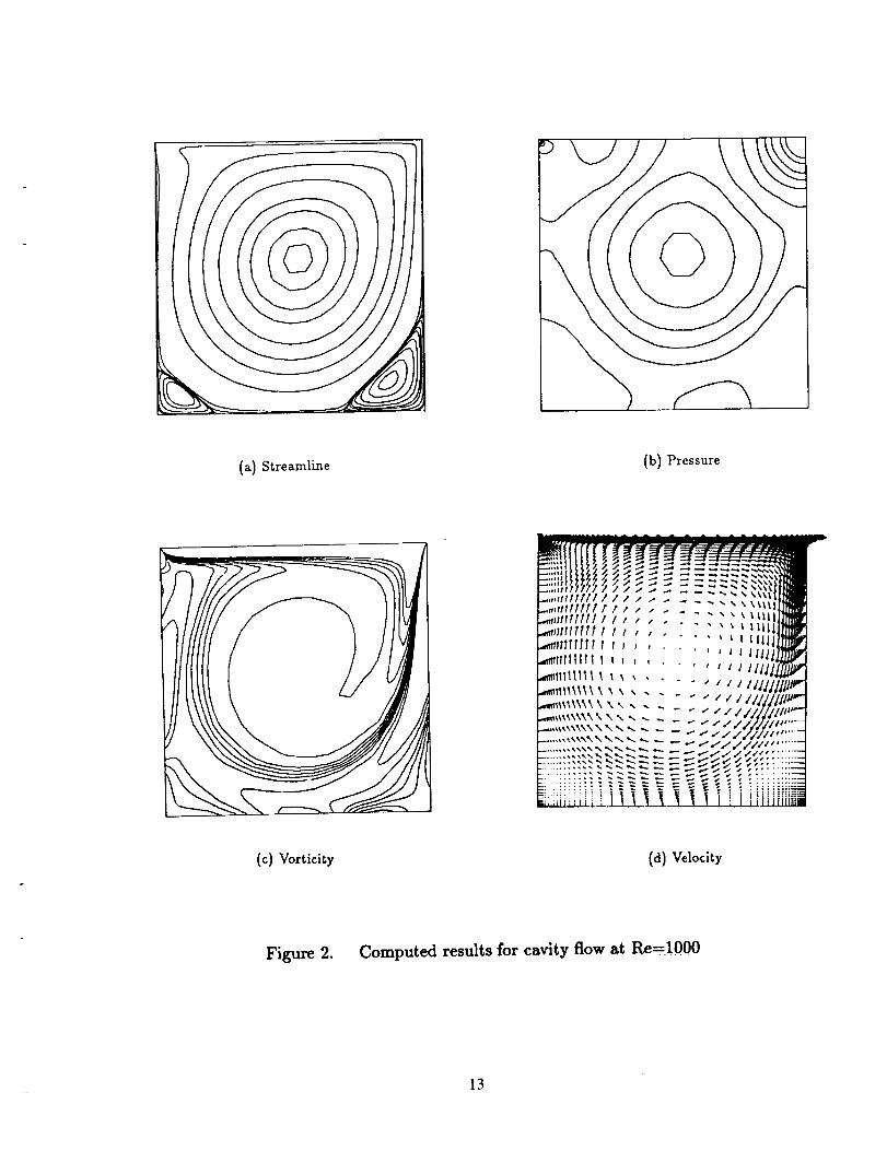
The computed results(streamlines, pressure contours, vorticity contours, and velocity
vectors) for Re = 1000,5000 and 10000 axe shown in Figure 2,3, and 4. Overall, the
streamlines and the vorticity contours compare rather well with those of Ghia et a/25
except for one region: the lower right eddy at Re --- 10000. The size and shape of this
small eddy compare more favorably with those of Gresho tt a/. 2e The pressure contours
compare well with those of Kim 27 and Sohn et a/. 12 The horizontal velocity profiles at
z = 0.5 compare well with those of Ghia et a/25 in Figure 5.
Backward-facing Step
This example is chosen to compare computational results with the experimental data
of Almaly eta/. 2s The step has a height of 0.0049m. The small channel, upstream of this
step, has a height of 0.0052m. the inlet boundary is located at 3.5 step heights upstream
of this step. The total length behind the backward-facing step is 45 step heights. A total
of 2550 nonuniform bilinear elements(6 × 15 for the smaller channel and 82 × 30 for the
larger channel) are used with fine meshes near the step. One point Gaussian quadratureis used to evaluate the element matrices.
A parabolic velocity profile with the center line velocity of 1.0m/s and a corresponding
vorticity are imposed at the inlet, v = 0, p = 0 are prescribed at the exit boundary, w = 0
is given at the lower step corner. The Reynolds number Re = U__p_Dis based on the hydraulicV
diameter(D = 0.0104m) of the inlet channel and the average velocity(v = 0.6667m/s). The
various Reynolds numbers are obtained by varying the kinematic viscosity v.
u = v = 0 is used as an initial guess for Re = 100, the converged solution for Re = 100
is used as an initial guess for Re = 200, and so on. The required numbers of substitutions
are 13,19,29,39,42,51,73,79, and 84 for the Reynolds number of 100 through 900 with the
incremental of 100, respectively. Under-relaxation is not used.
The computed results(streamlines, pressure contours, and vorticity contours) for Re =
400,500 and 800 are shown in Figure 6,7 and 8. The computed pressure is adjusted by
a constant such that p = 0 at the lower step corner. The reattachment length of the
recirculating zone behind the step and the location of detachment and reattachment of
another recirculating zone near the upper wall are compared with experimental data in
9

Figure 9, where zl is the reattachment location of the primary vortex, z4 is the separation
location of the secondary vortex at the top wall, z5 is the reattachment location of the
secondary vortex, and the distance is measured from the expansion step.
5. CONCLUSIONS
A new finite element method for incompressible Navier-Stokes problems is developed.
This method is simple, robust and reliable. This method represents a particular application
of a unified least-squares finite element method for first-order partial differential equations
in computational physics. Further developments are under way for solving 3D problems
and time-dependent problems. Theoretical investigation is also needed.
REFERENCES
1. P.S.Huyakorn, C.Taylor, R.L.Lee, and P.M.Gresho, A comparison of various mixed-
interpolation finite elements in the velocity-pressure formulation of the Navier-Stokes
equations,Computers and Fluids,6, 25-35(1978).
2. C.Taylor and T.G.Hughes,Finite Element Programming of the Navier-Stokes Equa-
tion, Pineridge Press, Swansea(1980).
3. G.F.Carey and J.T.Oden, Finite Elements: Fluid Mechanics, Vol.IV, Prentice-Hall(1986).
4. V.Girault and P.-A.Raviart, Finite Element Method for Navier-Stokes Equation, Springer-
Verlag(1986).5. C.Cuvelier, A.Segal and A.A.Van Steenhoven, Finite Element Methods and Navier-
Stokes Equations, D.Reidel Publishing Company(1986).
6. C.Taylor(editor), Finite-Element Applications in Fluid Mechanics, in Finite Element
Handbook,(editor-in-chief H.Kardestuncer), McGraw-Hill(1987).
7. I.Babu_ka, Error bounds for finite element method, Numer. Math.,16,322-333(1971).
8. F.Brezzi, On the existence, uniqueness and approximation of saddle-point problems
arising from Lagrange multipliers, Rech. Oper., Set. Rouge Anal. Numer.,8, R-
2,129-151(19 4).9. G.Comini and S.D.Giudice, Finite element solution of the compressible Navier-Stokes
equations, Numer. Heat Transfer, 5, 463-478(1982).
10. A.C.Benim and W.Zinser, A segregated formulation of Navier-Stokes equations with
finite elements, Comput. Meth. Appl. Mech. Engng., ST, 223-237(1986).
11. J.G.Rice and R.J.Schnipke, An equal-order veleocity-pressure formulation that does
not exibit spurious pressure modes. Comput. Meth. Appi. Mech. Engng., 58, 135-
149(19s6).12. J.L.Sohn, Y.Kim and T.J.Chung, Finite element solver for incompressible fluid flows
10

and heat transfer, in Finite Element Analysis in Fluids, (eds. T.J.Chung and G.R.Karr),
Proceedings of the Seventh International Conference on Finite Element Methods in
Flow Problems, UAH press, Huntsville, Alabama, 1989, pp.880-885.
13. B.N.Jiang and C.L.Chang, Least-squares finite elements for Stokes problem, Com-
put.Meth.Appl.Mech.Engrg.,(to appear); also available as NASA TM 101308, ICOMP-
88-16.
14. B.N.Jiang and L.A.Povinelli, Least-squares finite element method for fluid dynamics,
in Finite Element Analysis in Fluids, (eds. T.J.Chung and G.R.Karr), Proceedings of
the Seventh International Conference on Finite Element Methods in Flow Problems,
UAH press, Huntsville, Alabama, 1989, pp.105-110.
15. B.N.Jiang and L.A.Povinelli, A least-squares finite element method for incompress-
ible Navier-Stokes problem, in Proceedings of 12th Canadian Congress of Applied
Mechanics,(eds. M.A.Erki and J.Kirkhope), Carleton University, Ottawa, Ontario,
1989, pp.602-603.
16. C.L.Chang and B.N.Jiang, An error analysis of least-squares finite element method of
velocity-pressure-vorticity formulation for Stokes problem, Comput.Meth.Appl.Mech.
Engng., (submitted).
17. B.N.Jiang and L.A.Povinelli, Least-squares finite element method for fluid dynamics,
Comput. Meth. Appl. Mech. Engng., (to appear); also available as NASA TM 102352,
ICOMP-89-23.
18. G.F.Carey and J.T.Oden, Finite Elements: A Second Course, ,Vol. II, Prentice-Hall,
Englewood Cliffs, NJ,1983.
19. J.T.Oden and G.F.Carey, Finite Elements: Mathematical Aspects, Vol.IV, Prentice-
Hall, Englewood Cliffs, N J, 1983.
20. G.F.Carey and B.N.Jiang, Element-by-element linear and nonlinear solution schemes,
Communications in Applied Numerical Methods, 2, 145-153(1986).
21. G.F.Carey and E..I.Barragy, Parallel element-by-element solution scheme, Inter.J. Nu-
mer.Meth.Engng., 26, 2367-2382(1988).
22. A.K.Aziz, R.B.Kellogg and A.B.Stephens, Least-squares methods for elliptic systems,
Mathematics of Computation,44, 53-70(1985).
23. G.F.Carey and B.N.Jiang, Least-squares finite element method and preconditioned
conjugate gradient solution, [nter.J.Numer.Meth.Engng., 24, 1283-1296(1987).
24. E.D.Eason, A review of least-squares methods for solving partial differential equations,
Inter.J.Numer.Meth.Engng.,lO, 1021-1046(1976).
25. U.Ghia, K.N.Ghia and C.T.Shin, High-Re solutions for incompressible flow using the
Navier-Stokes equation and a multigrid method, J.Comput.Phys., 48, 387-411(1982).
26. P.M.Gresho, S.T.Chan, R.L.Lee and C.D.Upson, A modified finite element method
for solving the time-dependent incompressible Navier-Stokes equations, Part 2. appli-
cations, Inter.J.Numer.Meth.Fluids, 4, 619-640(1984).
27. S.W.Kim, A fine grid finite element computation of two-dimensional high Reynolds
number flows, Computers and Fluids, 16, 429-444(1988).
11

28. B.F.Armaly, F.Durst, J.C.F.Pereira and B.Schonung, Experimental and theoretical
investigationof b_kward-facing step flow, J.Flsid Mech.,127, 473-496(1982).
II
J
!I
Figure 1. Finite element mesh (50x50 bilinear elements) for the cavity flow
12
(a) Streamline(b) Pressure
_,rlrrrl r t, , ..... : : : _P,!!4_,.
- " _ _ / //l/]]lll#_
L
P
(c) Vorticity (d) Velocity
Figure 2. Computed results for cavity flow at Re=1000
13

(a) Streamline{b) Pressure
.....,#////'/z,......... ,....._I[]
-_t//llllll! ! I ,.,. - , , _ i..,ca//liMit/// _ . . , _ L,[],_llllllll/t t t I , , • , _ _11
" - " _ t tlllll_at_rlltttttr t t _ , ..... ,d_lIWI|II I _ , . , , _ | III|/ILll
• " " _ 1111111" " " /Z/Ill," " ," v v lltl_ _tl_"-_xxxxx__, , . ..... . /////r
.........._--_,._'x__.<...*-..... .,':_Z//_.-#J_./_'.::::::--Z
....... _ ._ _,___:_._-. _v.'L_'_ _ _ ............
(c)Vorticity (d) Velocity
Figure 3. Computed resultsfor cavityflow at Re=5000
14

(a) Streamline
(b) Pressure
(c) Vorticky(d} Velocity
Figure 4. Computed results for cavity flow at Re=10000
15

Re=7500 Re=5000 P,,e=3200 ]le=]O00 Re=400
C_, Re=f0000
co
___o'_o'. __ , , , o,.5, , , ,,,.oU
Figure 5. Horizontal velocity profile for cavity flow -- present, A Ghia et a/25
16

(a) Streamline
!J J
iI
(b) Pressure
(c) Vorticity
Figure 6. Computed Results for Backward-Facing Step Flow at Re=400.
17

_j
(a) Streamline
li __
(b) Pressure
(c) Vorticity
Figure 7. Computed Results for backward-Facing Step Flow at Re=500.
18

(a) Streamline
(b) Pressure
(c)Vorticlty
Figure 8. Computed Results for Backward-Facing Step Flow at Re=800
19

t.,..
t_",4
I,.,,..
t_t_
fM
(D
d"
¢kl
./
t/
//
/
oXs/h
j zl/h
x4/h
Figure 9.
I O0 200 I00 _00 500 600 700 800 900 1000
REYNOL OS NUMBER
Reattachment length vs Reynolds number for backward-facing step flow
p present, ZX, o, o: Exp't zl/h, z4/h, xs/h, respectively
2O

NationalAeronautics andSpace Administration
Report Documentation Page
1. Report No, NASA TM-i02385 [ICOMP-89-28 I
4. Title and Subtitle
2, Government Accession No. 3. Recipienrs Catalog No.
5. Report Date
A Least-Squares Finite Element Method for Incompressible Navier-Stokes Problems
7, Author(s)
Bo-nan Jiang
October 1989
6, Performing Organization Code
8, Performing Organization Report No.
E-5124
10. Work Unit No.
505-62-2 l
11. Contract or Grant No.
13. Type of Report and Period Covered
Technical Memorandum
14. Sponsoring Agency Code
9. Performing Organization Name and Address
National Aeronautics and Space AdministrationLewis Research Center
Cleveland, Ohio 44135-3191
12. Sponsoring Agency Name and Address
National Aeronautics and Space AdministrationWashington, D.C. 20546-0001
15. Supplementary Notes
Bo-nan Jiang, Institute for Computational Mechanics in Propulsion, Lewis Research Center, Cleveland, Ohio
44135 (work funded by Space Act Agreement C99066G). Space Act Monitor: Louis A. Povinelli.
16. Abstract
A least-squares finite element method, based on the velocity-pressure-vorticity formulation, is developed for
solving steady incompressible Navier-Stokes problems. This method leads to a minimization problem rather than
to a saddle-point problem by the classic mixed method, and can thus accommodate equal-order interpolations.This method has no parameter to tune. The associated algebraic system is symmetric, and positive definite.
Numerical results for the cavity flow at Reynolds number up to 10,000 and the backward-facing step flow at
Reynolds number up to 900 are presented.
17. Key Words (Suggested by Author(s))
Finite element; Least squares; Navier-Stokes equations;
First-order system; Velocity-pressure-vorticity; Equal-
order interpulations
Distribution Statement
Unclassified - Unlimited
Subject Category 64
2_. Security Classif, (of this page) r| 21. NO of pages19. Security Classif. (of this report)
Unclassified Unclassified 20/ /
NASA rOaM 162s oct a6 *For sale by the National Technical Information Service, Springfield, Virginia 22161
22. Price"
A03