-- N A S A TECHNICAL NOTE

w h M +? n z

A LEAST-SQUARE-DISTANCE CURVE-FITTING TECHNIQUE

by John Qs Howell

Langley Research Center Hampton, Vas 23365

N-ASA TN D-6374 - -I- 'c c

C, /

NATIONAL AERONAUTICS A N D SPACE ADMINISTRATION WASHINGTON, D. C. JULY 1971

c

https://ntrs.nasa.gov/search.jsp?R=19710021103 2018-05-22T10:58:11+00:00Z

- -

TECH LIBRARY KAFB, NM

1. Report No. 2. Government Accession No.

NASA TN D-6374 4. Title and Subtitle

A LEAST-SQUARE-DISTANCE CURVE-FITTING TECHNIQUE

7. Author(s)

John Q. Howell

9. Performing Organization Name and Address

NASA Langley Research Center Hampton, Va. 23365

-

2. Sponsoring Agency Name and Address

National Aeronautics and Space Administration Washington, D.C. 20546

6. Abstract

Illllll11111lllll11111llllllllllI1IllIll1HII 3. Recipient's Catalog No.

5. Report Date July 1971

6. performing organizationCode

8. Performing Organization Report No.

L-7675 10. Work Unit No.

125-21-21-01 11. Contract or Grant No.

13. Type of Report and Period Covered Technical Note

14. Sponsoring Agency Code

A method is presented for fitting a function with n pa rame te r s y = f(al,a2,. . .,CY,; x) t o a se t of N data points Gi,f$ in a manner that minimizes the sum of the squares of the distances f rom the data points t o the curve. A differential-correction scheme is used to solve for the parameters in an i terat ive manner until the best f i t is obtained. Two methods fo r finding the distances f rom the data points t o the curve and a listing of the curve-fitting com­puter program are a lso given.

7. Key Words (Suggested by Authoris))

Curve fitting Least-square distance Least squares

9. Security Classif. (of this report)

Unclassified - .

[ T8. Distribution Statement

Unclassified - Unlimited

I20. Security Classif. (of this page) 21. No. of Pager 22. Price*

Unclassified 24 $3.00

CONTENTS

Page SUMMARY . . . . . . . . . . . . . . . . . . . . . . . . . . . . . . . . . . . . . . . 1

INTRODUCTION . . . . . . . . . . . . . . . . . . . . . . . . . . . . . . . . . . . . 1

SYMBOLS . . . . . . . . . . . . . . . . . . . . . . . . . . . . . . . . . . . . . . . 2

DERIVATION AND DISCUSSION O F NEW TECHNIQUE . . . . . . . . . . . . . . . . 3

EXAMPLES O F APPLICATION O F NEW TECHNIQUE . . . . . . . . . . . . . . . . 6

CONCLUDING REMARKS . . . . . . . . . . . . . . . . . . . . . . . . . . . . . . . 9

APPENDIX A .TWO NUMERICAL METHODS FOR FINDING THE DISTANCE FROM A POINT TO A CURVE . . . . . . . . . . . . . . . . . . 13

APPENDIX B .COMPUTER PROGRAM FOR LEAST-SQUARE-DISTANCE TECHNIQUE . . . . . . . . . . . . . . . . . . . . . . . . . . . . 15

REFERENCES . . . . . . . . . . . . . . . . . . . . . . . . . . . . . . . . . . . . . 22

iii

.. 'Ill ll '..

A LEAST-SQUARE-DISTANCE CURVE-FITTING TECHNIQUE

By John Q. Howell Langley Research Center

SUMMARY

A method is presented for fitting a function with n parameters y = f(al,a2, . . .,an;x) to a set of N data points {Gi,yi) in a manner that mini­mizes the sum of the squares of the distances from the data points to the curve. A differential-correction scheme is used to solve for the parameters in an iterative man­ner until the best f i t is obtained. Two methods for finding the distances from the data points to the curve and a listing of the curve-fitting computer program a re also given.

INTRODUCTION

Most of the generally used methods of fitting a curve to a set of data points mini­mize a function of the vertical distances from the points to the curve. For example, if {Zi,ya is a set of N points and y = f(al,a2, . . .,an;x) is a curve with n, param­e ters , then the method of least squares gives values of the parameters that minimize

N

i=1

This may be done by taking partial derivatives with respect to the parameters and setting each of the resulting equations equal to zero; that is,

-N aE- = 0 = - 2 ( j = 1, 2 , . . ., n)a a

i=1

This set of n equations, sometimes called the normal equations, is then solved for the parameters. As is well known, if f is linear in the parameters, for example, a polynomial in x (ref. l),a set of simultaneous linear equations merely has t o be solved. However, in general, more complicated functions yield simultaneous equations that are

I - .-_

nonlinear. In this case f may be expanded in a truncated Taylor se r ies about a point in parameter space, and in this manner the nonlinear normal equations can be linearized and solved by iteration. The end result is a set of parameters that yields a minimum of equation (1). This is called either the Gauss-Newton method or the method of nonlinear least squares. However, when f(x) has a region where its derivative is large o r when both zi and yi have s imilar e r r o r bounds, it may be more desirable to minimize the distance from each data point to its nearest point on the curve. This minimum distance is the same as the perpendicular distance from the data point to the curve. Scarborough (ref. 2) gives a method for curve fitting that minimizes the sum of the squares of these distances but his method is limited to first-order polynomials. Reed (ref. 3) and Kendall and Stuart (ref. 4) give schemes that are applicable to polynomials of higher order. These same methods a r e useful fo r any function in which the parameters enter in a linear fashion. Guest (ref. 5) describes a related technique that minimizes the perpendicular distance from each data point to a straight line tangent to the curve. This tangent is taken at the point on the curve having the same x-coordinate as the data point.

The purpose of the present work is to derive and demonstrate the use of a curve-fitting technique that minimizes the least-square distances from each data point to the curve. The technique described herein works for a general function f and is most useful when the function being fitted contains regions where the slope is small as well as where the slope is large. It is also useful when the data points have e r ro r bounds asso­ciated with both the x- and y-coordinates. In the latter case, this technique implicitly assumes identical e r r o r for both coordinates. Generally the data points and the function can be scaled so that this condition is met. Other techniques that a r e less time con­suming may also be used in these situations. For example, a judicious choice of weights often makes possible the use of a standard least-squares procedure. However, in these cases a particular choice of weights seldom works for more than a few sets of data. The technique described herein does not have this disadvantage since it provides a fi t even when all the weights a r e set equal to 1.

SYMBOLS

defined by equation (10)

defined by equation (9)

distance from (%i,Yi)to nearest point on curve, equations (4) and (16)

value of Di using old parameters, equation (6)

2

distance from (?i,fi) to some point on curve, equation (17)

sum of squares of distances f rom data points to curve, equations (1)and (3)

function to be fitted to data points; y = f(x)

value of function at iii, equation (2)

value of function at xi with old parameters, equation (8)

number of function parameters

number of data points

weight associated with data point (zi,yi)

coordinates of one data point of set to which y = f(x) is being fitted

coordinates of point on curve nearest data point (Zi,ui)

* . ,an parameters of y = f(x)

A .,an old parameters of y = f(x) during iteration t o find least-square­distance fit

root-mean-square deviation of data points from curve, equation (14)

DERIVATION AND DISCUSSION O F NEW TECHNIQUE

There is given a set of N data points (Si,?$ t o which is to be fitted the function y = f(al,a2,. . .,an; x), where a l , a 2 , . . .,an a r e parameters. To obtain this f i t the sum of the least-square distances (sum of the squares of the shortest distances) from the data points to the curve must be minimized. By using one of the techniques given in appendix A, the coordinates (xi,yi) a r e found fo r the point on the curve that is nearest each data point (.zi,yi). Then it is desired to minimize

3

where the distance from the ith data point to the curve is

The weight t o be associated with each point is given by Wi. To minimize equation (3) it is necessary to solve the set of n normal equations

( j = 1, 2 , . . ., n) (5)

In general this is a set of nonlinear simultaneous equations. To solve the set , an iterative procedure sometimes called the method of differential correction can be used. First a Taylor se r ies expansion of Di is made about some point (&1,6~,. . .,&) in parameter space. Since Di is a known function of the parameters, the expansion can easily be written

and

Now in equation (6) all higher order te rms a re dropped and only the te rms that a r e linear in Aa a r e kept. Then substitution of equation (6) into equation (5) gives

(j = 1, 2, . . .,n)

Also, equation (4) yields

where

4

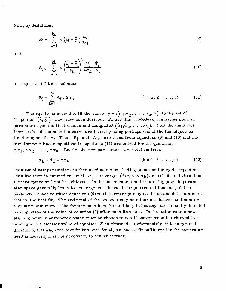
Now, by definition,

and

and equation (7) then becomes

n

Bj = 1Ajk ACYk (j = 1, 2 , . . .,n) (11) k=1

The equations needed to f i t the curve y = f(al,a2,. . .,an; x) to the set of N points {?i,y$ have now been derived. To use this procedure, a starting point in parameter space is first chosen and designated (&1,g2,. . .,&n). Next the distances from each data point t o the curve a r e found by using perhaps one of the techniques out­lined in appendix A. Then Bj and Ajk are found from equations (9) and (10) and the simultaneous linear equations in equations (11) a r e solved for the quantities A a l , ha2, . . .,A@,. Lastly, the new parameters a r e obtained from

( k = 1, 2, . . ., n) (12)

This set of new parameters is then used as a new starting point and the cycle repeated. This iteration is carried out until (ilk converges ( h a k <<< a k ) o r until it is obvious that a convergence will not be achieved. In the latter case a better starting point in param­eter space generally leads to convergence. It should be pointed out that the point in parameter space to which equations (9) t o (11) converge may not be an absolute minimum, that is, the best f i t . The end point of the process may be either a relative maximum o r a relative minimum. The former case is rather unlikely but at any rate is easily detected by inspection of the value of equation (3) after each iteration. In the latter case a new starting point in parameter space must be chosen to see if convergence is achieved t o a point where a smaller value of equation (3) is obtained. Unfortunately, it is in general difficult t o tell when the best f i t has been found, but once a f i t sufficient for the particular need is located, it is not necessary to search farther.

5

EXAMPLES OF APPLICATION OF NEW TECHNIQUE

The two examples given herein a r e chosen to demonstrate that for some cases the least-square-distance curve-fitting technique gives better results than the standard least-squares method, The first example arose when the author was trying t o reduce some experimental plasma-physics data and led ultimately to the least-square-distance curve-fitting technique described in this paper, The second example is chosen since it is commonly known that standard least-squares procedures do not work well on this type of function. For the examples presented here the weights a re set equal to one. By prop­er ly choosing the weights it may be possible to obtain a f i t with the least-squares tech­nique that is as good as that obtained with the least-square-distance method. However, for a different function and often for a different set of data points, a new set of weights would have to be chosen to achieve a good f i t again. The least-square-distance technique described in this report does not have this disadvantage.

Because of the extra computations involved in finding the closest point on the ‘curve, the least-square-distance method takes more computer time than the least-squares method. Based on the following two examples it is determined that the least-square­distance method is longer by a factor of approximately 2.5.

Example I

Example I is taken from the field of plasma physics where a common diagnostic tool is the Langmuir probe. The current versus voltage characteristic of this probe is given approximate1y by

y = a1x2 + a2x + a3 + a4e 5x

where x is the voltage, y is the current, and a1,a2, . . .,a5 a r e a set of adjustable parameters. The parameters a 4 and a 5 a re always positive so the exponential t e rm is large for x positive and small for x negative.

When the Langmuir probe is used as a diagnostic tool, the current is typically mea­sured for a large set of voltage points. Then some curve-fitting technique is used to obtain a f i t to the experimental data. The value of a5 is of interest as the electron temperature can be obtained from it. This temperature is then used to calculate a par­ticular voltage in the region where the exponectial t e rm is small and the fitted function is used to obtain the corresponding current. The ion density can then be obtained from this current. From this description it is apparent (1)that both x and y may be in e r r o r and (2) the f i t to the experimental data must be good both in regions where the exponential t e rm is large and where it is small.

6

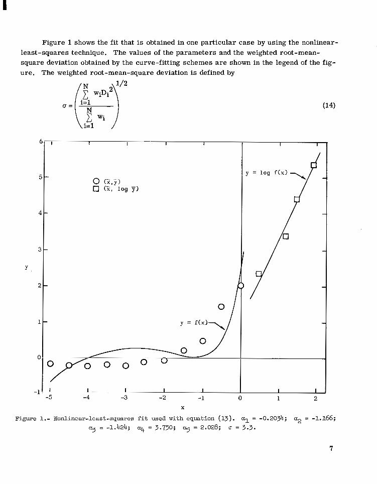
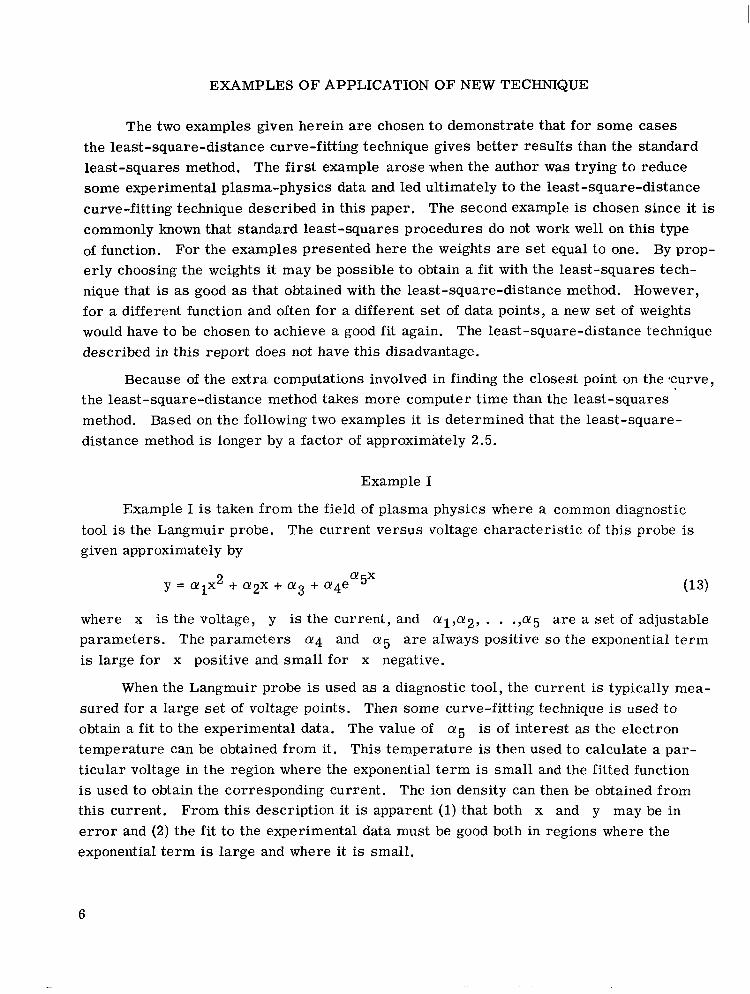
Figure 1 shows the f i t that is obtained in one particular case by using the nonlinear­least-squares technique. The values of the parameters and the weighted root-mean­square deviation obtained by the curve-fitting schemes a r e shown in the legend of the fig­ure. The weighted root-mean-square deviation is defined by

( T =

t I I I I I

5

4

3

y .

2

1 y = f(x1 \O/

o / 0

-1 I I 1 I I -5 -4 -3 -2 -1 0 1 2

X

Figure 1.- Nonlinear-least-squares fit used with equation (13) . = -0.2034; a2 = -1.166; = -1.424; u4 = 3.750; as = 2.028; u = 3.3.

7

where Di is the vertical distance in the case of the least-squares technique and the shortest distance from the point to the curve for the least-square-distance method. The least-squares f i t for x negative is not acceptable (fig. 1)but the fi t is good for x posi­tive where the exponential t e rm is large.

The same set of data points is then used in a program based on the least-square­distance technique derived in the present paper. The result of this f i t is shown in fig­ure 2. It is immediately apparent that the fit’is much better and is in fact good enough to extract the desired information for the further data analysis as described earlier. The legends of figures 1and 2 show that only a5 agrees to within 20 percent. As

5

4

3

Y

2

1

0

-1 -5

- 1 I I

J I I I I 1 1 -4 -3 -2 -1 0 1 2

X

Figure 2.- Least-square-distancefit used with equation (13) and same data points as in figure 1. al = 0.05013; a2 = 0.3994; a3 = 0.5654; a4 = 2.398; 9= 2.2611; G = 0.077.

8

would be expected from a comparison of figures 1 and 2, the coefficients of the polyno­mial portion of the function are in violent disagreement. The reason the least-squares technique does not do so well is that it finds a f i t that is good in the high-slope and high-magnitude region at the expense of the f i t in the small-slope and small-magnitude region.

Example 11

Example II is chosen t o show that the least-square-distance curve-fitting technique fits functions with a singularity. The function chosen is

y = a1x3 + a2x2 + a3x + a4 + -a5 x - 25

In figure 3 the results of the nonlinear-least-squares curve-fitting scheme are shown. The values of the parameters and the weighted root-mean-square deviation of the points from the curve are shown in the legend of the figure. The least-square­distance fit of the same function to the same points is shown in figure 4. A s in example I , the f i t to the small-magnitude points is better when the least-square-distance technique is used while both methods give s imilar fits for the large-magnitude points. In example I1 the initial parameter guess for the least-square-distance method is more critical than usual. With a bad initial guess both distance-finding techniques described in appendix A sometimes achieve convergence to a point on the wrong side of the singu­lari ty. This can also happen if the fitting function has a very sharp peak, in which case the distance-finding scheme may achieve convergence to a point on the wrong side of the peak. Of course, if it is desired to f i t a function of this type to several sets of data, the program can be designed to alleviate this problem, but the fitting routine has to be dif­ferent for each particular function.

CONCLUDING REMARKS

In the present paper the least-square-distance curve-fitting method is derived and examples of its use a r e presented. This technique fits a function with n parameters y = f{al,a2,. . .,an; x) to a set of N data points ei,y$by minimizing the sum of the squares of the distances from the data points to the curve. A differential-correction scheme is used to solve for the parameters in an iterative manner until the best f i t is obtained. Two examples of the use of this technique a r e presented, both involving func­tions having large slope variations. In both cases the least-squares f i t is found to be lacking when compared to the least-square-distance f i t . It is found that the least-squares technique fits the curve to points in the regions of large slope and large magnitude at the expense of the f i t in regions of small slope and small magnitude. This does not happen for the least-square-distance method presented in this paper since the sum of the squares

9

14 I

12 0 ( X t Y )

10

8

6

4

2

Y O

-2

-4

-6

-8

-10

-12

-14

0

-

P7y’lo

I I 0 10 20 30 40 50

Figure 3 . - Nonlinear-least-squaresfit used with equation (15). a1 = O.OOO8l9; = -0.06442; a3 = 0.9939; a4 = 3.886; a5 = -12.75; 0 = 2.6.

10

. .-. ..

10 30 40 502o x

Figure 4.- Least-square-distance fit used with e q u a t i a (155)and same data points as i n figure 3 . ul = 0.000709; u2 = -0.03129; u3 = 0.5789; “4 = 6.147; u5 = -14.04; CI = 0.21.

11

of the distances from the data points to the curve is minimized. Hence, for functions of this type the least-square-distance technique fits a function to a set of points more accu­rately than the least-squares method, unless much time is spent in customizing the least-squares weights to the particular function and particular set of data.

Langley Research Center, National Aeronautics and Space Administration,

Hampton, Va., June 10, 1971.

12

APPENDIX A

TWO NUMERICAL METHODS FOR FINDING THE DISTANCE

FROM A POINT TO A CURVE

In appendix A two methods a re presented for finding the distance from the data point (Zi,yi) to the curve y = f(x). The first method minimizes the distance from the curve to the data point, while the second method finds the perpendicular from the curve to the data point. Both these methods locate the point on the curve k i , f ( X i g nearest the data point. The distance from the data point to the curve is then given by

For some very simple cases this point can be found analytically but the assumption is made here that f(x) is of such complexity that this is impossible.

Method I

The distance from some point on the curve y = f(x) to the data point ( is

Di(x) = ([f(x) - fd2 + (X - %i)2)1'2 Now an x such that Di is minimum may be found by solving

mi 0-= dx

For the case of Di # 0 (for Di = 0, the trivial solution is xi = Zi and yi = yi), it is seen from equation (18) that xi must satisfy the equation

Once xi is found, yi is obtained from yi = f(xi), and equation (16) is used to find Di. Equation (19) can be solved by any convenient method. For cases where the second derivative of f(x) is obtainable, the author has used the Newton-Raphson method with good success. It should be kept in mind that in some cases the solution of equation (19) may yield a Di that is a relative maximum or a relative minimum instead of the abso­lute minimum that is desired. Fortunately these cases a r e rare.

13

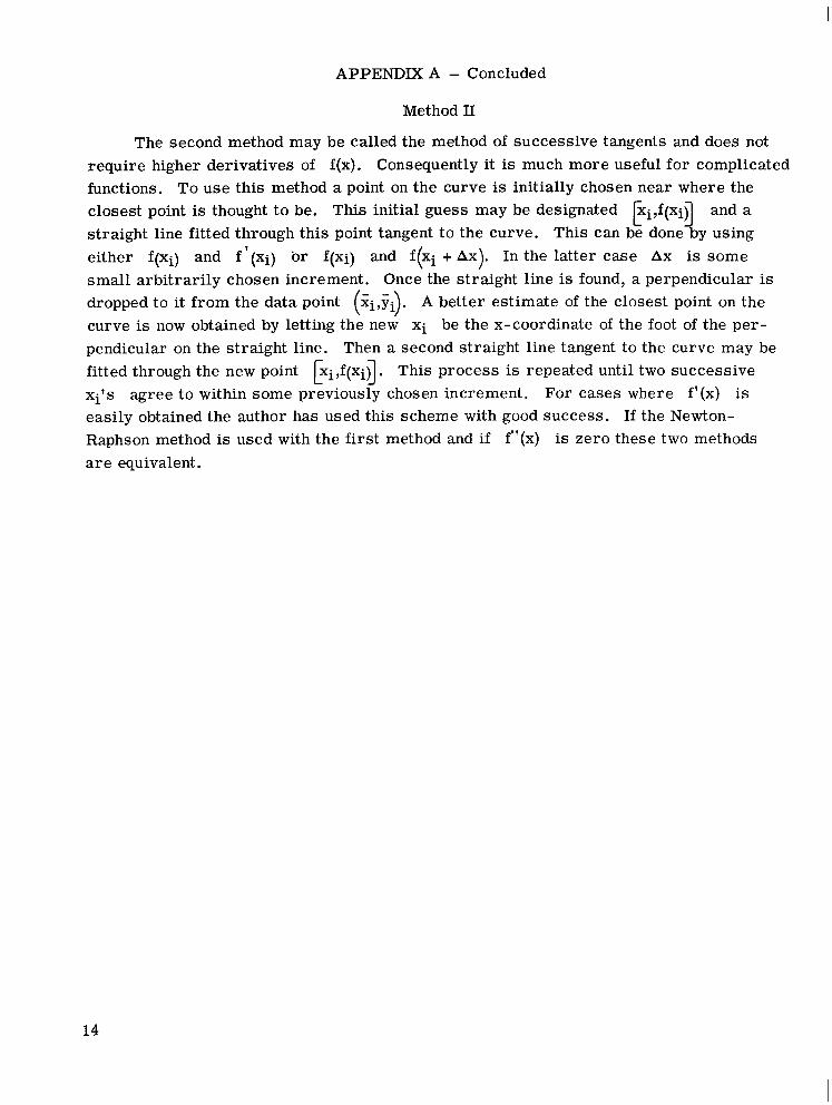
APPENDIXA - Concluded

Method II

The second method may be called the method of successive tangents and does not require higher derivatives of f(x). Consequently it is much more useful for complicated functions. To use this method a point on the curve is initially chosen near where the closest point is thought t o be. This initial guess may be designated Lki,f(xifl and a straight line fitted through this point tangent to the curve. This can be done by using either f(xi) and f ' ( X i ) or f(xi) and f(xi + A x ) . In the latter case Ax is some small arbitrari ly chosen increment. Once the straight line is found, a perpendicular is dropped to it from the data point (%i,fi). A better estimate of the closest point on the curve is now obtained by letting the new X i be the x-coordinate of the foot of the per­pendicular on the straight line. Then a second straight line tangent to the curve may be fitted through the new point ki,f(xi)l. This process is repeated until two successive xi's agree to within some previously chosen increment. For cases where f'(x) is easily obtained the author has used this scheme with good success. If the Newton-Raphson method is used with the first method and if f"(x) is zero these two methods a r e equivalent.

14

APPENDIX B

COMPUTER PROGRAM FOR LEAST-SQUARE -DISTANCE TECHNIQUE

Appendix B contains a description and listing of a least-square-distance curve-fitting program written in FORTRAN. The procedure for finding the distance from the data point t o the curve is built into the curve-fitting subroutine. The method used is the successive-tangent method described in appendix A. The curve-fitting subroutine also has a damping procedure (ref. 6) included for increased stability. This program has operated satisfactorily for the author with several different functions but has not been tested extensively.

Main Program

It is felt that a description of the main program is not needed since any potential user has to write the main program around his own particular application.

Least-Square-Distance C:irve- Fitting Subroutine

This subroutine assumes the existence of a linear-simultaneous-equation solver called SIMSOL. It is called by the statement

Call SIMSOL(A,B,M)

and solves the equation in M unknowns given by AX=B. The solution vector for X is returned in B. The curve-fitting subroutine also calls the subroutine FUNC described subsequently. A description of the calling procedure for the curve-fitting subroutine follows.

Use: Call LSD(X,Y,W,N,AL,M,ERR,RMS)

Vectors containing x- and y-coordinates of data points to which function Y”> is being fitted.

W Vector containing weight associated with each point.

N The number of points being supplied to subroutine by main program.

AL Vector containing values of function parameters. Initially a trial set must be supplied. The curve-fitting subroutine iterates and returns a better set.

M The number of parameters in function being fitted.

15

I

APPENDIX B - Continued

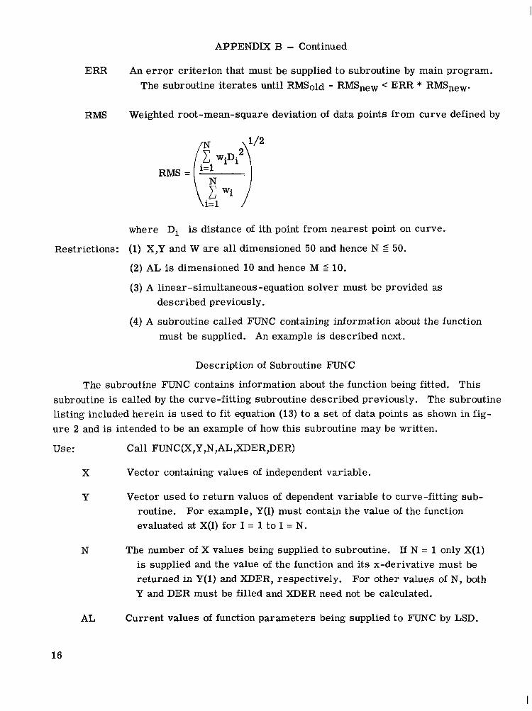
ERR An e r r o r criterion that must be supplied t o subroutine by main program. The subroutine i terates until RMSold - RMSnew < ERR * RMSnew.

RMS Weighted root-mean-square deviation of data points from curve defined by

where Di is distance of ith point from nearest point on curve.

Restrictions: (1) X,Y and W a re all dimensioned 50 and hence N 2 50.

(2) AL is dimensioned 10 and hence M 5 10.

(3) A linear-simultaneous -equation solver must be provided as described previously.

(4) A subroutine called FUNC containing information about the function must be supplied. An example is described next.

Description of Subroutine FUNC

The subroutine FUNC contains information about the function being fitted. This subroutine is called by the curve-fitting subroutine described previously. The subroutine listing included herein is used to f i t equation (13) to a set of data points as shown in fig­ure 2 and is intended t o be an example of how this subroutine may be written.

Use: Call FUNC(X,Y ,N,AL , D E R ,DE R)

X Vector containing values of independent variable.

Y Vector used to return values of dependent variable to curve-fitting sub­routine. For example, Y(1) must contain the value of the function evaluated at X(1) for I = 1 to I = N.

N The number of X values being supplied to subroutine. If N = 1 only X(l) is supplied and the value of the function and its x-derivative must be returned in Y(l)and XDER, respectively. For other values of N, both Y and DER must be filled and D E R need not be calculated.

AL Current values of function parameters being supplied to FUNC by LSD.

16

XDER

DER

Restrictions:

APPENDIX B - Continued

Variable containing value of x-derivative of function evaluated at X(1). It need be calculated only when N = 1.

Matrix containing derivatives of function with respect to all function parameters, each evaluated at X(I), for I = 1to I = N. This matrix must be filled by FUNC whenever N > 1. The defining equation is

where aK is Kth function parameter.

(1) X and Y a r e dimensioned 50 so N 6 50.

(2)AL is dimensioned 10.

(3)DER is dimensioned (10,50).

17

APPENDIX B - Continued

C C C C C M A I N PROGRAM C C C C THIS PROGRAM R E A D S THE I N I T I A L G U E S S A T THE P A R A M E T E R S A N D THE D A T A

C P O l N T S AND THEN C A L L S THE L E A S T S Q U A R E D I S T A N C E C U R V E F I T T E R . C C

PROGRAM C F I T ( I N P U T r 0 U T P U T ) D I M E N S I O N X ( 5 O ) . Y ( 5 0 ) . W ( 5 0 ) r A L ( l O ) E R R = 1 E-5

1 R E A D 1 0 0 0 r M 1 ( A L ( I ) r I = l r M ) 1000 F O R M A T ( I 2 r / ( E I O ) )

R E A D 10BlrN~(X(I)rY(I)rW(I)rI~l*N) 1001 F O R M A T ( I 2 / ( 3E10 ) )

C A L L L S D ( X r Y r W r N r A L r M r E R R I R M S ) GO T O 1 END

C C C C C L E A S T S Q U A R E D I S T A N C E C U R V E F I T T I N G S U B R O U T I N E

C C c C

SUBROUT I NE L S D ( X I Y W Nr A L r M ERR* RMS ) C C T H I S I S A L E A S T S Q U A R E OJSTANCE C U R V E F I T T I N G S U B R O U T I N E . C I T H A S B U I L T I N THE S U C E S S f V E T A N G E N T L INE SCHEME T O FIND THE C D I S T A N C E FROM A D A T A P O I N T T O THE CURVE. C I T C A L L S S I M S O L ( A * B r M ) T O S O L V E T H E L I N E A R S I M U L T A N E O U S E Q U A T I O N

c A X = B I N M UNKNOWNS.

C I T C A L L S FU N C T O O B T A I N I N F O R M A T I O N A B O U T T H E F U N C T I O N B E I N G F I T T E D . D!MENSI O N X ~ 5 0 ) r Y ~ 5 O ~ r W ~ 5 ~ ) r A L ~ l 0 ) r D ~ 1 0 ~ 5 0 ) ~ B ~ 1 0 ~ ~ A ~ 1 0 ~ 1 0 ~ D IMENS I O N D I S t 5 0 ~ ~ X 1 ~ 5 0 ~ r W 2 ~ 5 0 ~ r l D ( 2 ~ r Y 1 ( S O ) . D X ~ 5 0 ~

C C I F IPRINT=OI T H E R E I S NO P R I N T E O O U T P U T F R O M T H I S S U B R O U T I N E *

I P R I N T = O I PR I NT= 2 T R M S = l *E10 I D ( 1 ) = 1 OHCONVERGED I D ( E ) = I O H D O 2 I C l r N

2 DX(I)=O* C C S T A R T T T E R A T I O N

D O 100 I T E R = l r 100 C C F I N D C L O S E S T P O I N T S O N C U R V E

5 DO 30 I=frN w 2 c I) = w ( I P

18

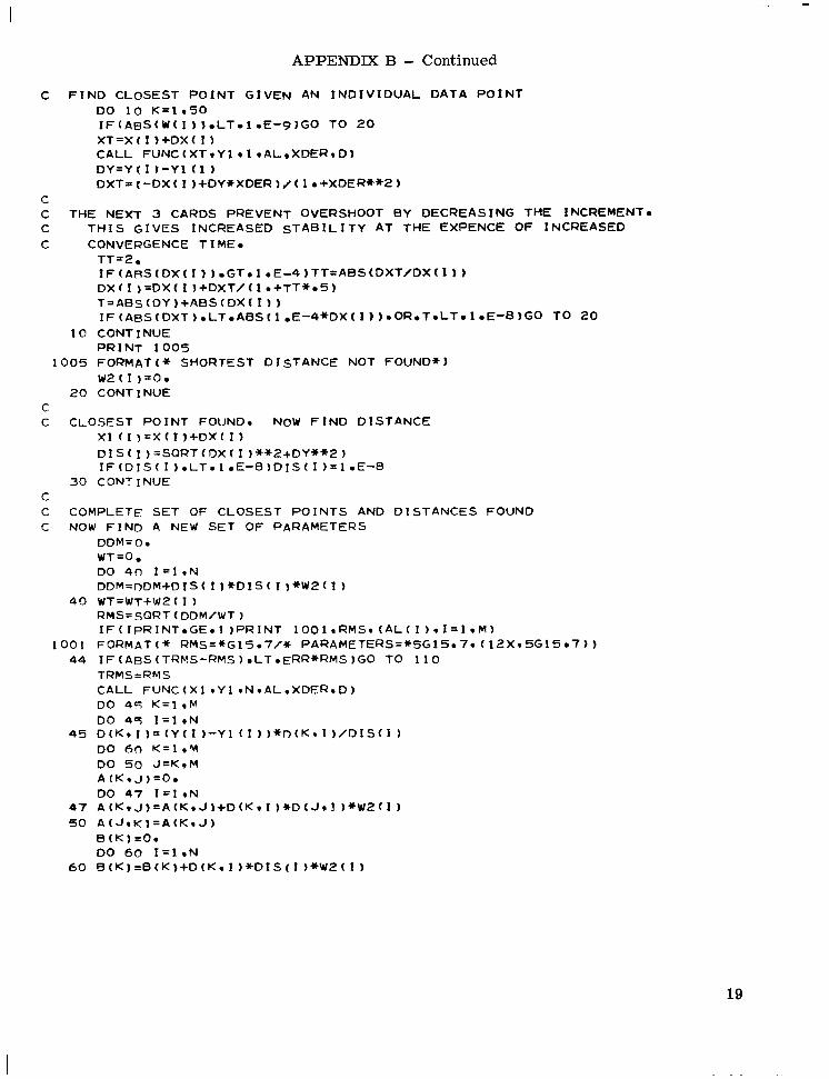
APPENDIX B - Continued

C F IND C L O S E S T P O I N T G I V E N A N I N D I V I D U A L D A T A P O I N T DO 10 K Z l . 5 0 I F ( A B S ( W ( I ) ) . L T . I . E - 9 ) C O T O 20 X T = X ( I ) + D X ( I ) C A L L F U N C ( X T * Y l r l r A L * X D E R I D ) D Y = Y ( I ) - Y I ( 1 1 D X T ~ ( - D X ( I ) + D Y * X D E R ) / ( I . + X D E R + + 2 )

C C THE NEXT 3 CARDS PREVENT OVERSHOOT B Y D E C R E A S I N G THE INCREMENT. C T H I S G I V E S I N C R E A S E D S T A B I L I T Y A T THE E X P E N C E OF I N C R E A S E D

C CONVERGENCE T I M E . T T = 2 . I F ( A R S ( D X ( I ) ) . G T . I . E - ~ ) T T ~ A ~ S ~ D X ( I ) ) DX(I)=DX(I)+DXT/(l.+TT**5) T = A B S ( O Y ) + A B S ( D X ( I ) ) IF(A~S(DXT)~LTeABS(l~E-4*DX(X))~OR~T~LT~l~E-8)GO T O 20

10 C O N T I N U E P R I N T 1005

1005 F O R M A T ( * S H O R T E S T D I S T A N C E N O T F O U N D * ) w 2 ( I )=0.

20 CONT 1NU� C C C L O S E S T P O I N T FOUND. NOW F IND D I S T A N C E

x1 ( I ) = x ( I ) + D x ( I ) DIS(I)=SQRT(DX(I)**2+DY**2) I F ( D I S ( I ) . L T . I . E - B ) D T S o z l . E - 8

30 CONTINUE C C C O M P L E T E S E T OF C L O S E S T P O I N T S AND D l S T A N C E S F O U N D C NOW FIND A NEW S E T O F P A R A M E T E R S

40

I001 44

45

47 50

60

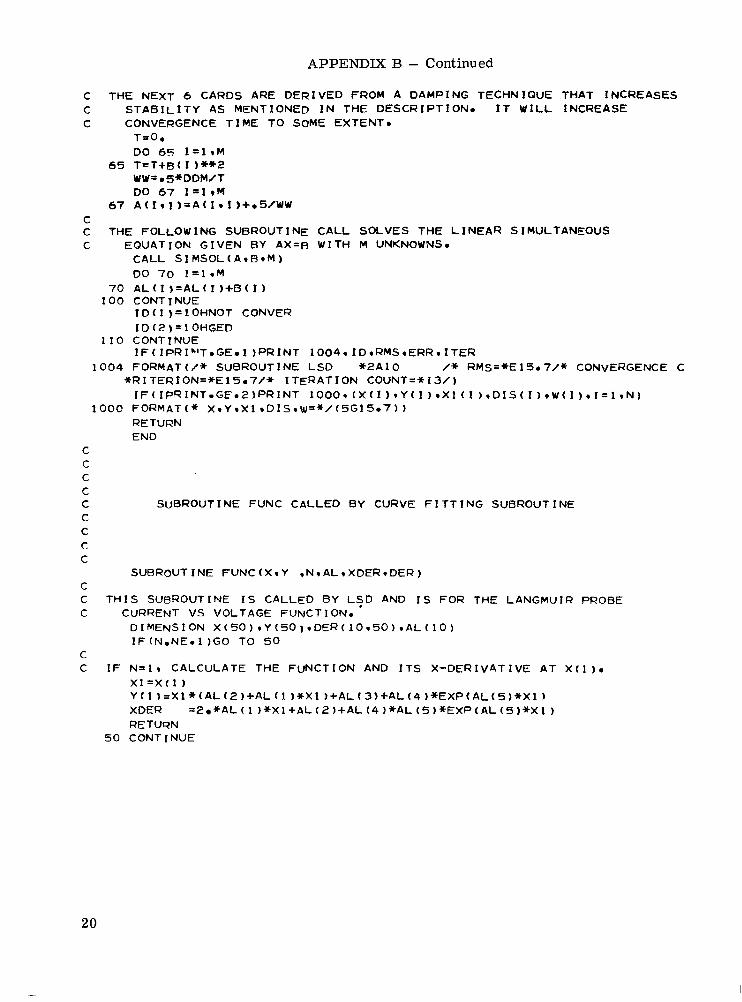
APPENDIX B - Continued

C THE NEXT 6 CARDS ARE D E R I V E D FROM A D A M P I N G T E C H N I Q U E THAT INCREASES C S T A B I L I T Y AS MENTIONED I N THE D E S C R I P T I O N . IT W I L L INCREASE C CONVERGENCE T I M E T O SOME EXTENT.

T x O o DO 65 I = l r M

65 T=T+B( I )**2 UU=.S*DDM/T DO 67 I = l * M

67 A ( I * I ) = A ( I * I ) + o 5 / W W C C THE FOLLOWING SUBROUTINE C A L L SOLVES T H E L I N E A R SIMULTANEOUS C E Q U A T I O N G I V E N B Y AX=B W I T H M UNKNOWNS.

C A L L S I M S O L ( A * B * M ) DO 70 I = l * M

70 A L < I ) = A L ( I)+E< 1 1 100 C O N T I N U E

I D ( 1 ) = 1OHNOT CONVER 1D(2)=1OHGED

110 C O N T I N U E I F ( I P R I " T . G E . l ) P R I N T 1 0 0 4 * I D * R M S * E R R * I T E R

1004 FORMAT( / * SUBROUTINE L S D * 2 A 1 0 /* R M S = * E 1 5 * 7 / * CONVERGENCE C * R I T E R I O N = * E l 5 ~ 7 / * I T E R A T I O N C O U N T = * I J / )

I F ( I P R I N T . G E . 2 ) P R I N T 1 0 0 0 ~ ~ X ~ I ~ * Y ~ I ~ ~ X 1 ~ I ~ ~ D I S ~ I ~ ~ W ~ I ) ~ I ~ l ~ N ) 1000 FORMAT(* X ~ Y I X ~ ~ D I S ~ W = * / ( ~ G I S O ~ ) )

RETURN END

C C C C C SUBROUTINE FUNC C A L L E D B Y CURVE F I T T I N G SUBROUTINE C C C C

SUBROUTINE F U N C ( X * Y * N * A L * X D E R * D E R )

C T H I S SUBROUTINE IS C A L L E D B Y L ? D AND IS FOR THE LANGMUIR PROBE C CURRENT VS VOLTAGE FUNCTION.

D I M E N S I O N X(50)rY(5O)rDER(10~5O)~AL(lO) I F ( N o N E * I )GO TO 50

C IF N n l r CALCULATE THE F U N C T I O N AND I T S X - D E R I V A T I V E A T X ( 1 ) . x l = x ( l ) Y ( 1 ) = X I * ( A L ( 2 )+AL ( 1 ) + X I ) + A L ( 3 ) + A L ( 4 ) *EXP( A L ( 5 ) * X l 1 XDER =2 * A L ( 1 1 *X 1+ A L ( 2 1 + A L (41 *AL ( 5 ) *EXP ( A L ( 5 )*X 1 ) RETUQN

50 C O N T I N U E

20

APPENDMB - Concluded

C IF N NOT = l r CALCULATE THE F U N C T I O N AND D E R I V A T I V E S WITH RESPECT C TO A L L PARAMETERS AT P O I N T S X ( I ) * I = l r N *

DO In0 I=I*N x I = x ( I ) T I = E x P ( A L ( S ) * X l ) T = A L ( ~ ) * T I x2=x 1*x 1 Y ( I ) =AL ( 1 )*XE+AL ( 2) * X I +AL (3)+T DER ( l * I ) = X 2 DER ( 2 * I ) = X 1 DER ( 3 * I ) = l * DER ( 4 r I ) = T l DER ( 5 9 I ) = X l * T

100 CONTINUE RETURN END

21

REFERENCES

1. Nielsen, Kaj L.: Methods in Numerical Analysis. Macmillan Co., c.1956.

2. Scarborough, James B.: Numerical Mathematical Analysis. Second ed., John Hopkins Press, 1950.

3. Reed, Frank C.: A Method of Least Squares Curve Fitting With Error in Both Variables. NAVORD Rep. 3521, US.Navy, June 1955.

4. Kendall, Maurice G.; and Stuart, Alan: The Advanced Theory of Statistics. Vol. 2 -Inference and Relationship. Hafner Pub. Co., Inc., c.1961, p. 409.

5. Guest, P. G.: Numerical Methods of Curve Fitting. Cambridge Univ. P res s , 1961, p. 366.

6. Levenberg, Kenneth: A Method for the Solution of Certain Non-Linear Problems in Least Squares, Quart. Appl. Math., vol. 11, no. 2, July 1944, pp. 164-168.

22 NASA-Langley, 1971 - 19 L-7675

NATIONAL AND SPACE ADMINISTRATAERONAUTICS ION

WASHINGTON,D. C. 20546

OFFICIAL BUSINESS FIRST CLASS MAIL PENALTY FOR PRIVATE USE $300

POSTAGE A N D FEES PAID NATIONAL AERONAUTICS A%

SPACE ADMINISTRATION

003 001 C1 U 19 710716 S00903DS DEPT nf THE A I R FORCE ME APnN S LABnRRTORY / W t O L / ATTN: E L O U BOWMAN, CHIEF T E C H L I B R A R Y K I R T L A N O A F R NM 87117

P O S ~ ~ ~ S T ~ ~ :If Undeliverable (Section 158 Postal Manual) Do Nor Recur.

- *

“The aeronaatical and space activities of the United Stntes shall be conducted so as to contribute . . . to the expansion of human knowl­edge of phenomena in the atmosphere and space. T h e Adniinistration shall provide for the widest prncticable and appropriate dissemination of information concerning i ts activitiei and the resdts thereof.”

-NATIONALAERONAUTICSAND SPACE ACT OF 1958

NASA SCIENTIFIC AND TECHNICAL PUBLICATIONS

TECHNICAL REPORTS: Scientific and technical information considered important, complete, and a lasting contribution to existing knowledge.

TECHNICAL NOTES: Information less broad in scope but nevertheless of importance as a contribution to existing knowledge.

TECHNICAL MEMORANDUMS: Information receiving limited distribution because of preliminary data, security classifica­tion, or other reasons.

CONTRACTOR REPORTS: Scientific and technical information generated under a NASA contract or grant and considered an important contribution to existing knowledge.

TECHNICAL TRANSLATIONS: Information published in a foreign language considered to merit NASA distribution in English.

SPECIAL PUBLICATIONS: Information derived from or of value to NASA activities. Publications include conference proceedings, monographs, data compilations, handbooks, sourcebooks, and special bibliographies.

TECHNOLOGY UTILIZATION PUBLICATIONS: Information on technology used by NASA that may be of particular interest in commercial and other non-aerospace applications. Publications include Tech Briefs, Technology Utilization Reports and Technology Surveys.

Details on fhe availability of these publications may be obtained from:

SCIENTIFIC AND TECHNICAL INFORMATION OFFICE

NATIONAL AERONAUTICS AND SPACE ADMINISTRATION Washington, D.C. PO546