Embed Size (px)
Citation preview

Research Article Vol. 1, No. 1 / July 2014 / Optica 1
A Learning Approach to Optical TomographyULUGBEK S. KAMILOV*,1, IOANNIS N. PAPADOPOULOS*,2, MORTEZA H.SHOREH*,2, ALEXANDRE GOY2, CEDRIC VONESCH1, MICHAEL UNSER1, ANDDEMETRI PSALTIS**,2
*These authors contributed equally to the paper1Biomedical Imaging Group, Ecole polytechnique federale de Lausanne, Switzerland2Optics Laboratory, Ecole polytechnique federale de Lausanne, Switzerland**Corresponding author: [email protected]
Compiled April 24, 2015
Optical tomography has been widely investigated for biomedical imaging applications. In re-cent years optical tomography has been combined with digital holography and has been em-ployed to produce high quality images of phase objects such as cells. In this paper we describea method for imaging 3D phase objects in a tomographic configuration implemented by trainingan artificial neural network to reproduce the complex amplitude of the experimentally measuredscattered light. The network is designed such that the voxel values of the refractive index of the3D object are the variables that are adapted during the training process. We demonstrate themethod experimentally by forming images of the 3D refractive index distribution of Hela cells.© 2014 Optical Society of America
OCIS codes: (180.1655) Coherence tomography; (180.3170) Interference microscopy, (180.6900) Three-dimensional microscopy,(100.3010) Image reconstruction techniques.
http://dx.doi.org/10.1364/optica.XX.XXXXXX
1. INTRODUCTION
The learning approach to imaging we describe in this paper isrelated to adaptive techniques in phased antenna arrays [1], it-erative imaging schemes [2, 3], and inverse scattering [4, 5]. Inthe optical domain an iterative approach was demonstrated bythe Sentenac group [6, 7] who used the coupled dipole approx-imation [8] for modeling light propagation in inhomogeneousmedia (a very accurate method but computationally intensive)to simulate light scattering from small objects (1µm ⇥ 0.5µm)in a point scanning microscope configuration. Maleki and De-vaney in 1993 [9] demonstrated diffraction tomography usingintensity measurements and iterative phase retrieval [10]. Veryrecently an iterative optimization method was demonstrated[11] for imaging 3D objects using incoherent illumination andintensity detection. There are similarities but also complemen-tary differences between our method and [11]. Our method usescoherent light and relies on digital holography [12, 13] to recordthe complex amplitude of the field whereas direct intensity de-tection is used in [11]. Both use the Beam Propagation Method(BPM) [14, 15] to model the scattering process and the error backpropagation method [16] to train the system. At the end of the
training process the network discovers a 3D index distributionthat is consistent with the experimental observations. We exper-imentally demonstrate the technique by imaging polystyrenebeads and HeLa and hTERT-RPE1 cells.
The holographic recording employed in the method pre-sented in this paper are advantageous for imaging phase objectssuch as the cells in the experiments. Moreover we included inthis optimization algorithm sparsity constraints which improvesignificantly the quality of the reconstructions. We also com-pared our method to other coherent tomographic reconstructiontechniques. The learning approach improved the quality ot theimages produced by all the direct (non-iterative) tomographicreconstruction methods we tried.
2. EXPERIMENTAL SETUP
A schematic diagram of the experimental setup is shown in Fig-ure 1. It is a holographic tomography system [17], in which thesample is illuminated with multiple angles and the scatteredlight is holographically recorded. Several variation of the holo-graphic tomography system have been demonstrated before[18–21]. The optical arrangement we used is most similar to the
Research Article Vol. 1, No. 1 / July 2014 / Optica 2
He-NeLaser
GM
BS1
L1OB1 OB2
L2 BS2
M
CMOS
SampleL3
L4
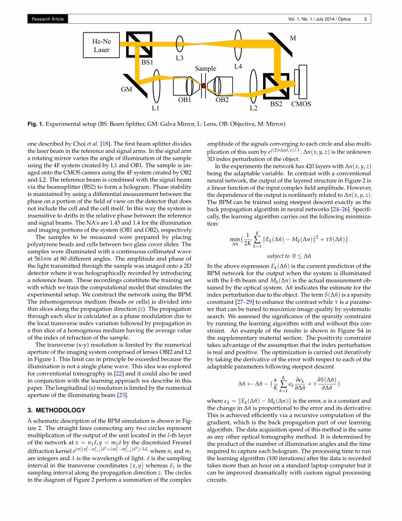
Fig. 1. Experimental setup (BS: Beam Splitter, GM: Galva Mirror, L: Lens, OB: Objective, M: Mirror)
one described by Choi et al. [18]. The first beam splitter dividesthe laser beam in the reference and signal arms. In the signal arma rotating mirror varies the angle of illumination of the sampleusing the 4F system created by L1 and OB1. The sample is im-aged onto the CMOS camera using the 4F system created by OB2and L2. The reference beam is combined with the signal beamvia the beamsplitter (BS2) to form a hologram. Phase stabilityis maintained by using a differential measurement between thephase on a portion of the field of view on the detector that doesnot include the cell and the cell itself. In this way the system isinsensitive to drifts in the relative phase between the referenceand signal beams. The NA’s are 1.45 and 1.4 for the illuminationand imaging portions of the system (OB1 and OB2), respectively.
The samples to be measured were prepared by placingpolystyrene beads and cells between two glass cover slides. Thesamples were illuminated with a continuous collimated waveat 561nm at 80 different angles. The amplitude and phase ofthe light transmitted through the sample was imaged onto a 2Ddetector where it was holographically recorded by introducinga reference beam. These recordings constitute the training setwith which we train the computational model that simulates theexperimental setup. We construct the network using the BPM.The inhomogeneous medium (beads or cells) is divided intothin slices along the propagation direction (z). The propagationthrough each slice is calculated as a phase modulation due tothe local transverse index variation followed by propagation ina thin slice of a homogenous medium having the average valueof the index of refraction of the sample.
The transverse (x-y) resolution is limited by the numericalaperture of the imaging system comprised of lenses OBJ2 and L2in Figure 1. This limit can in principle be exceeded because theillumination is not a single plane wave. This idea was exploredfor conventional tomography in [22] and it could also be usedin conjunction with the learning approach we describe in thispaper. The longitudinal (z) resolution is limited by the numericalaperture of the illuminating beam [23].
3. METHODOLOGY
A schematic description of the BPM simulation is shown in Fig-ure 2. The straight lines connecting any two circles representmultiplication of the output of the unit located in the l-th layerof the network at x = n1d, y = m1d by the discretized Fresneldiffraction kernel ejp[(n2
l�n2l+1)d
2+(m2l�m2
l+1)d2]/ldz where nl and ml
are integers and l is the wavelength of light. d is the samplinginterval in the transverse coordinates (x, y) whereas dz is thesampling interval along the propagation direction z. The circlesin the diagram of Figure 2 perform a summation of the complex
amplitude of the signals converging to each circle and also multi-plication of this sum by ej(2pDndzz)/l. Dn(x, y, z) is the unknown3D index perturbation of the object.
In the experiments the network has 420 layers with Dn(x, y, z)being the adaptable variable. In contrast with a conventionalneural network, the output of the layered structure in Figure 2 isa linear function of the input complex field amplitude. However,the dependence of the output is nonlinearly related to Dn(x, y, z).The BPM can be trained using steepest descent exactly as theback propagation algorithm in neural networks [24–26]. Specifi-cally, the learning algorithm carries out the following minimiza-tion:
minDn
{ 12K
K
Âk=1kEk(Dn)�Mk(Dn)k2 + tS(Dn)}
subject to 0 Dn
In the above expression Ek(Dn) is the current prediction of theBPM network for the output when the system is illuminatedwith the k-th beam and Mk(Dn) is the actual measurement ob-tained by the optical system. Dn indicates the estimate for theindex perturbation due to the object. The term S(Dn) is a sparsityconstraint [27–29] to enhance the contrast while t is a parame-ter that can be tuned to maximize image quality by systematicsearch. We assessed the significance of the sparsity constraintby running the learning algorithm with and without this con-straint. An example of the results is shown in Figure S4 inthe supplementary material section. The positivity constrainttakes advantage of the assumption that the index perturbationis real and positive. The optimization is carried out iterativelyby taking the derivative of the error with respect to each of theadaptable parameters following steepest descent
Dn Dn�� a
K
K
Âk=1
ek∂ek∂Dn
+ t∂S(Dn)
∂Dn�
where ek = kEk(Dn)�Mk(Dn)k is the error, a is a constant andthe change in Dn is proportional to the error and its derivative.This is achieved efficiently via a recursive computation of thegradient, which is the back propagation part of our learningalgorithm. The data acquisition speed of this method is the sameas any other optical tomography method. It is determined bythe product of the number of illumination angles and the timerequired to capture each hologram. The processing time to runthe learning algorithm (100 iterations) after the data is recordedtakes more than an hour on a standard laptop computer but itcan be improved dramatically with custom signal processingcircuits.

Research Article Vol. 1, No. 1 / July 2014 / Optica 3
Δф
Δф
Δф
Δф
Δф
Δф
Δф
Δф
Δф | ε|²
| ε|²
| ε|²
Error = | ε|²Error Correction
Expe
rim
enta
l Mea
sure
men
t
Inci
dent
Fie
ld
Propagation Δф Phase Modulation
BPM Model
+
+
+
-
-
-
Fig. 2. Schematic diagram of object reconstruction by learning the 3D index distribution that minimizes the error e, defined at themean squared difference between the experimental measurement and the prediction of a computational model based on the beampropagation method (BPM).
4. RESULTS
We first tested the system with polystyrene beads encapsulatedbetween two glass slides in immersion oil. The sample wasinserted in the optical system of Figure 1 and 80 hologramswere recorded by illuminating the sample at 80 distinct anglesuniformly distributed in the range -45 degrees to +45 degrees.The collected data is the training set for the 420-layer BPM net-work which simulates a physical propagation distance of 30µmand transverse window 37µm⇥ 37µm (dx = dy = 72nm). Thenetwork was initialized with the standard filtered back projec-tion reconstruction algorithm (Radon transform) [30] and theresulting 3D images before and after 100 iterations are shown inFigure 3. The final image produced by the learning algorithm isan accurate reproduction of the bead shape.
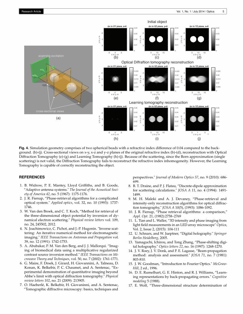
The power of the learning tomography method presentedin this paper is that the reconstruction of the refractive index isnot based on the Born approximation. The beam propagationmethod does not account for reflections but it allows multipleforward scattering events. In case of multiple inhomogeneities,the Born approximation is not valid anymore and the reconstruc-tion based on conventional tomographic techniques becomeinaccurate. In order to demonstrate this effect, we simulate arefractive index inhomogeneity (Dn = 0.04, D = 5µm) that com-prises of two spherical beads on the optical axis at two differentz-planes. Considering the center of the computational windowto be the center of the x-y plane, the center of the beads areplaced at, x1 = 0 µm, y1 = 0 µm, z1 = 6 µm and x2 = 0 µm,y2 = 5 µm, z2 = 12 µm at a distance of 6µm away from eachother. Figure 4 shows the results of the two different reconstruc-tion schemes. Based on our previous explanation, since the Bornapproximation is not valid to describe the physical behaviour
(a) (b) (c)
(d) (e) (f)
10µm
Fig. 3. Experimental reconstruction of two 10µm beads ofrefractive index 1.588 at l = 561nm in immersion oil withn0 = 1.516. (a)-(c) x-y, y-z and x-z slices using the inverseRadon transform reconstruction, (d)-(f) the same slices for ourlearning based reconstruction method (The lines indicate thelocation of the slices).
of light propagation through this sample, the optical diffractiontomography method is not capable of reconstructing the object.Contrary to that, the Learning Tomography method presentedin this paper is capable of dealing with multiple scattering andtherefore correctly reconstructs the object.
A sample of a HeLa cell was also prepared and the same pro-cedure was followed to obtain a 3D image. The results are shownin Figure 5 where the error function is plotted as a function of
Research Article Vol. 1, No. 1 / July 2014 / Optica 4
iteration number. In this instance, the system was initializedwith a constant but nonzero value (Dn = 0.007). Also shown inFigure 5 are the results obtained when the system was initializedwith the Radon reconstruction from the same data. After 100 it-erations both runs yield essentially identical results. Notice thatthe error in the final image (after 100 iterations) is significantlylower than to the error of the Radon reconstruction. This is alsoevident by visual inspection of the images in Figure 5 wherethe artifacts due to the missing cone [31] and diffraction [18] areremoved by the learning process.
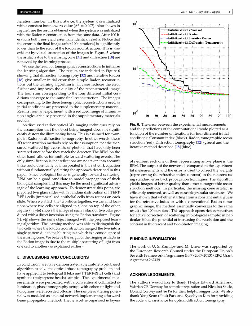
We use the result of tomographic reconstructions to initializethe learning algorithm. The results are included in Figure 6showing that diffraction tomography [32] and iterative Radon[18] give smaller initial error than simple Radon reconstruc-tions but the learning algorithm in all cases reduces the errorfurther and improves the quality of the reconstructed image.The four runs corresponding to the four different initial con-ditions converge to the same final reconstruction. The imagescorresponding to the three tomographic reconstructions used asinitial conditions are presented in the supplementary material.Results from an experiment with a reduced range of illumina-tion angles are also presented in the supplementary materialssection.
As discussed earlier optical 3D imaging techniques rely onthe assumption that the object being imaged does not signifi-cantly distort the illuminating beam. This is assumed for exam-ple in Radon or diffraction tomography. In other words, these3D reconstruction methods rely on the assumption that the mea-sured scattered light consists of photons that have only beenscattered once before they reach the detector. The BPM, on theother hand, allows for multiple forward scattering events. Theonly simplification is that reflections are not taken into account;these could eventually be incorporated in the network equationwithout fundamentally altering the approach described in thispaper. Since biological tissue is generally forward scattering,BPM can be a good candidate to model propagation of thickbiological samples and this may be the most significant advan-tage of the learning approach. To demonstrate this point, weprepared two glass slides with a random distribution of hTERT-RPE1 cells (immortalized epithelial cells from retina) on eachslide. When we attach the two slides together, we can find loca-tions where two cells are aligned in z, one on top of the other.Figure 7 (a)-(e) shows the image of such a stack of two cells pro-duced with a direct inversion using the Radon transform. Figure7 (f)-(j) shows the same object imaged with the proposed learn-ing algorithm. The learning method was able to distinguish thetwo cells where the Radon reconstruction merged the two into asingle pattern due to the blurring in z which is a consequence ofthe missing cone. We believe the origin of the ringing artifacts inthe Radon image is due to the multiple scattering of light fromone cell to another (as explained earlier).
5. DISCUSSIONS AND CONCLUSIONS
In conclusion, we have demonstrated a neural-network basedalgorithm to solve the optical phase tomography problem andhave applied it to biological (HeLa and hTERT-RPE1 cells) andsynthetic (polystyrene beads) samples. The experimental mea-surements were performed with a conventional collimated il-lumination phase tomography setup, with coherent light andholograms were recorded off-axis. The sample scattering poten-tial was modeled as a neural network implementing a forwardbeam propagation method. The network is organised in layers
Fig. 6. The error between the experimental measurementsand the predictions of the computational mode plotted as afunction of the number of iterations for four different initialconditions: Constant index (black), Radon tomographic recon-struction (red), Diffraction tomography [32] (green) and theiterative method described [18] (blue) .
of neurons, each one of them representing an x-y plane in theBPM. The output of the network is compared to the experimen-tal measurements and the error is used to correct the weights(representing the refractive index contrast) in the neurons us-ing standard error back propagation techniques. The algorithmyields images of better quality than other tomographic recon-struction methods. In particular, the missing cone artefact isefficiently removed, as well as parasitic granular structures. Wehave shown that whether starting from a constant initial guessfor the refractive index or with a conventional Radon tomo-graphic image, the method essentially converges to the sameresult after 100 iterations. This approach opens rich perspectivesfor active correction of scattering in biological sample; in par-ticular, it has the potential of increasing the resolution and thecontrast in fluorescent and two-photon imaging.
FUNDING INFORMATION
The work of U. S. Kamilov and M. Unser was supported bythe European Research Council under the European Union’sSeventh Framework Programme (FP7/2007-2013)/ERC GrantAgreement 267439.
ACKNOWLEDGEMENTS
The authors would like to thank Phelps Edward Allen andValerian CR Dormoy for sample preparation and Nicolino Stasio,Donald Conkey and Ye Pu for their helpful suggestions. We alsothank YongKeun (Paul) Park and Kyoohyun Kim for providingthe code and assistance for optical diffraction tomography.
Research Article Vol. 1, No. 1 / July 2014 / Optica 5
scanning excitation
cross-sectional views
Δn in XZ plane, y=0
z in µ m5 10 15
x in
µ m
-5
0
5
0
0.01
0.02
0.03
0.04 Δn in YZ plane, x=0
z in µ m5 10 15
y in
µ m
-5
0
5
0
0.01
0.02
0.03
0.04 Δn in XY plane, z=0
x in µ m-5 0 5
y in
µ m
-5
0
5
0
0.01
0.02
0.03
0.04
Initial object
Δn in XZ plane, y=0
z in µ m5 10 15
x in
µ m
-5
0
5
0
0.01
0.02
0.03
0.04
0.05 Δn in YZ plane, x=0
z in µ m -65 1 5
y in
µ m
-5
0
5
0
0.01
0.02
0.03
0.04
0.05 Δn in XY plane, z=0
x in µ m-5 0 5
y in
µ m
-5
0
5
0
0.01
0.02
0.03
0.04
0.05
Learning tomography reconstruction
x in µ m-5 0 5
y in
µ m
-5
0
5
Δn in XY plane, z=0 Δn in YZ plane, x=0
y in
µ m
-5
0
5
Δn in XZ plane, y=0
z in µ m5 10 15
x in
µ m
-5
0
5
Optical Diffraftion tomography reconstruction
(b) (c) (d)
(e) (f) (g)
(h) (i) (j)
(a)
0
0.005
0.01
0.015
0.02
0.025
z in µ m5 10 15
0
0.005
0.01
0.015
0.02
0.025
0
0.005
0.01
0.015
0.02
0.025
Fig. 4. Simulation geometry comprises of two spherical beads with a refractive index difference of 0.04 compared to the back-ground. (b)-(j). Cross-sectional views on x-y, x-z and y-z planes of the original refractive index (b)-(d), reconstruction with OpticalDiffraction Tomography (e)-(g) and Learning Tomography (h)-(j). Because of the scattering, since the Born approximation (singlescattering) is not valid, the Diffraction Tomography fails to reconstruct the refractive index inhomogeneity. However, the LearningTomography is capable of correctly reconstructing the object.
REFERENCES
1. B. Widrow, P. E. Mantey, Lloyd Griffiths, and B. Goode,“Adaptive antenna systems." The Journal of the Acoustical Soci-ety of America 42, no. 5 (1967): 1175-1176.
2. J. R. Fienup, “Phase-retrieval algorithms for a complicatedoptical system." Applied optics, vol. 32, no. 10 (1993): 1737-1746.
3. W. Van den Broek, and C. T. Koch, “Method for retrieval ofthe three-dimensional object potential by inversion of dy-namical electron scattering." Physical review letters vol. 109,no. 24, 245502, 2012.
4. N. Joachimowicz, C. Pichot, and J.-P. Hugonin. "Inverse scat-tering: An iterative numerical method for electromagneticimaging." IEEE Transactions on Antennas and Propagation vol.39, no. 12 (1991): 1742-1753.
5. A. Abubakar, P. M. Van den Berg, and J. J. Mallorqui. “Imag-ing of biomedical data using a multiplicative regularizedcontrast source inversion method." IEEE Transactions on Mi-crowave Theory and Techniques, vol. 50, no. 7 (2002): 1761-1771.
6. G. Maire, F. Drsek, J. Girard, H. Giovannini, A. Talneau, D.Konan, K. Belkebir, P. C. Chaumet, and A. Sentenac, “Ex-perimental demonstration of quantitative imaging beyondAbbe’s limit with optical diffraction tomography." Physicalreview letters 102, no. 21 (2009): 213905.
7. O. Haeberlé, K. Belkebir, H. Giovaninni, and A. Sentenac,“Tomographic diffractive microscopy: basics, techniques and
perspectives." Journal of Modern Optics 57, no. 9 (2010): 686-699.
8. B. T. Draine, and P. J. Flatau, “Discrete-dipole approximationfor scattering calculations." JOSA A 11, no. 4 (1994): 1491-1499.
9. M. H. Maleki and A. J. Devaney, “Phase-retrieval andintensity-only reconstruction algorithms for optical diffrac-tion tomography," JOSA A 10(5), (1993): 1086-1092.
10. J. R. Fienup, “Phase retrieval algorithms: a comparison,”Appl. Opt. 21, (1982):2758–2769
11. L. Tian and L. Waller, “3D intensity and phase imaging fromlight field measurements in an LED array microscope" Optica,Vol. 2, Issue 2, (2015): 104-111
12. U. Schnars, and W. Jueptner, “Digital holography." SpringerBerlin Heidelberg, 2005.
13. Yamaguchi, Ichirou, and Tong Zhang, “Phase-shifting digi-tal holography." Optics letters 22, no. 16 (1997): 1268-1270.
14. J. V. Roey, J. V. Donk, and P. E. Lagasse, “Beam-propagationmethod: analysis and assessment." JOSA 71, no. 7 (1981):803-810.
15. J. W. Goodman, “Introduction to Fourier Optics." McGraw-Hill, 2 ed., 1996.
16. D. E. Rumelhart, G. E. Hinton, and R. J. Williams, “Learn-ing representations by back-propagating errors." Cognitivemodeling 5 (1988).
17. E. Wolf, “Three-dimensional structure determination of

Research Article Vol. 1, No. 1 / July 2014 / Optica 6
(b) (f)
(c) (g)
(d)
10 Iterations 10 Iterations
1 Iteration1 Iteration
100 Iterations
x-y
y-z
x-z
(h)
100 Iterations
y-z
x-zx-y
(a) (e)
Fig. 5. Comparison of the proposed method initialized with the inverse Radon transform (left) versus initialization with a constantvalue (Dn = 0.007) (right). Figures (a) and (e) plot the error fall-off for 80 illumination angles initialized with the inverse Radon andconstant value, respectively. The horizontal doted line shows the inverse Radon performance for comparison. (b)-(d), x-y, y-z andx-z stacks for respectively the first, tenth and hundredth iteration of the proposed method initialized by inverse Radon. (d)-(f), thesame figures for the proposed method initialized by constant value.
semi-transparent objects from holographic data." Optics Com-munications 1, no. 4 (1969): 153-156.
18. W. Choi, C. Fang-Yen, K. Badizadegan, S. Oh, N. Lue, R.R. Dasari, and M. S. Feld, “Tomographic phase microscopy,”Nat. Methods, vol. 4, (2007): 717–719.
19. W. Choi, C. Fang-Yen, K. Badizadegan, R. R. Dasari, andM. S. Feld, “Extended depth of focus in tomographic phasemicroscopy using a propagation algorithm." Optics letters 33,no. 2 (2008): 171-173.
20. Y. Sung, W. Choi, C. Fang-Yen, K. Badizadegan, R. R. Dasari,and M. S. Feld, “Optical diffraction tomography for highresolution live cell imaging," Opt. Express, vol. 17, (2009):266–277.
21. F. Charrière, A. Marian, F. Montfort, J. Kuehn, T. Colomb,
E. Cuche, P. Marquet, and C. Depeursinge, “Cell refractiveindex tomography by digital holographic microscopy." Opticsletters 31, no. 2 (2006): 178-180.
22. Y. Cotte, F. Toy, P. Jourdain, N. Pavillon, D. Boss, P. Mag-istretti, P. Marquet, and C. Depeursinge, “Marker-free phasenanoscopy," Nat. Photonics, vol. 7, no. 2, pp. 113–117, Jan.2013.
23. V. Lauer, “New approach to optical diffraction tomographyyielding a vector equation of diffraction tomography anda novel tomographic microscope" Journal of Microscopy, Vol.205, Pt 2 February 2002, pp. 165–176
24. A. Beck, and M. Teboulle, “Gradient-based algorithms withapplications to signal recovery." Convex Optimization in SignalProcessing and Communications (2009).

Research Article Vol. 1, No. 1 / July 2014 / Optica 7
(a)10 µm
(b)
(c)
(d)
(e)
(f)
(g)
(h)
(i)
(j)
1.341.351.361.371.38
Fig. 7. Images of two hTERT-RPE1 cells. x-y slices correspond-ing to different depths of respectively +9, +6, +3, 0 and -3 mi-crons (positive being toward the detector) from the focal planeof the lens OB2 in Figure 1 for: (a)-(e) the inverse Radon trans-form based reconstruction and (f)-(j) the same slices for ourlearning based reconstruction method.
25. L. Bottou, “Neural Networks: Tricks of the Trade," ch.Stochastic Gradient Descent Tricks, Springer, 2 ed., (2012):421–437.
26. C. M. Bishop, “Neural Networks for Pattern Recognition."Oxford, 1995.
27. E. J. Candes, M. B. Wakin, and S. P. Boyd, “Enhancing spar-sity by reweighted l1 minimization," J. of Fourier Anal. Appl.,vol. 14, (2008): 877–905.
28. E. Y. Sidky, M. A. Anastasio, and X. Pan, “Image reconstruc-
tion exploiting object sparsity in boundary-enhanced X-rayphase-contrast tomography." Optics express vol. 18, no. 10 pp.10404-10422, 2010.
29. Lustig, Michael, David Donoho, and John M. Pauly. "SparseMRI: The application of compressed sensing for rapid MRimaging." Magnetic resonance in medicine 58, no. 6 (2007):1182-1195.
30. R. M. Lewitt, “Reconstruction algorithms: transform meth-ods." Proceedings of the IEEE, vol. 71, no. 3 (1983): 390-408.
31. V. Lauer, “New approach to optical diffraction tomographyyielding a vector equation of diffraction tomography and anovel tomographic microscope." Journal of Microscopy 205, no.2 (2002): 165-176.
32. K. Kim, H. Yoon, M. Diez-Silva, M. Dao, R. R. Dasari, andY. Park, “High-resolution three-dimensional imaging of redblood cells parasitized by Plasmodium falciparum and in situhemozoin crystals using optical diffraction tomography.,” J.Biomed. Opt., vol. 19, p. 011005, 2014