A learner’s P1−FEM code

Francisco–Javier SayasUniversity of Delaware

Last update: March 11, 2015

Contents

1 The triangulation and its data structure 2

2 How to create a mesh using the PDE Toolbox 3

3 A reordered mesh 5

4 The expanded data structure 5

5 Stiffness and mass matrices 7

6 Load and traction 10

7 Evaluation of the gradient 12

8 L2 and H1 errors 13

9 A simple PDE solver 15

10 Edge numbering 16

11 Uniform (red) refinement of a triangulation 18

12 Newest Vertex Bisection 19

13 Variable coefficients and boundary mass 21

Foreword. Many of the ideas of this program/document are borrowed from the following technicalreport of the Technical University of Vienna:

S. Funken, D. Praetorius, P. Wissgott. Efficient implementation of adaptive P1-FEM inMATLAB

The above document deals with adaptivity (which I won’t) in the two dimensional setting. I’ll try toexplain things directly and you’ll very easily see how to change the type of finite element, because mostof the information related to the particular finite element is given in the data structure and in the localmatrices on the reference element. The treatment of source terms and Neumann boundary conditionswill be developed only for the lowest order elements.

1

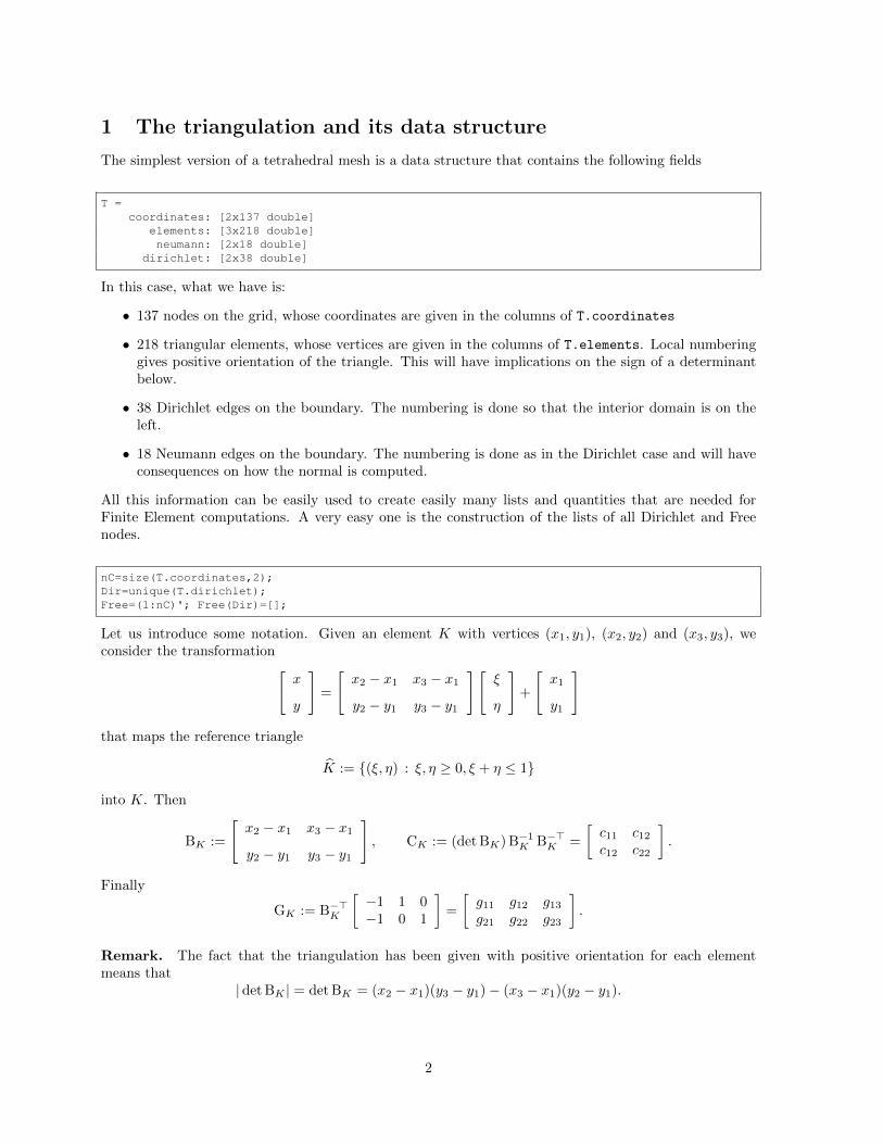
1 The triangulation and its data structure

The simplest version of a tetrahedral mesh is a data structure that contains the following fields

T =coordinates: [2x137 double]

elements: [3x218 double]neumann: [2x18 double]

dirichlet: [2x38 double]

In this case, what we have is:

• 137 nodes on the grid, whose coordinates are given in the columns of T.coordinates

• 218 triangular elements, whose vertices are given in the columns of T.elements. Local numberinggives positive orientation of the triangle. This will have implications on the sign of a determinantbelow.

• 38 Dirichlet edges on the boundary. The numbering is done so that the interior domain is on theleft.

• 18 Neumann edges on the boundary. The numbering is done as in the Dirichlet case and will haveconsequences on how the normal is computed.

All this information can be easily used to create easily many lists and quantities that are needed forFinite Element computations. A very easy one is the construction of the lists of all Dirichlet and Freenodes.

nC=size(T.coordinates,2);Dir=unique(T.dirichlet);Free=(1:nC)'; Free(Dir)=[];

Let us introduce some notation. Given an element K with vertices (x1, y1), (x2, y2) and (x3, y3), weconsider the transformation[

x

y

]=

[x2 − x1 x3 − x1

y2 − y1 y3 − y1

][ξ

η

]+

[x1

y1

]

that maps the reference triangle

K := (ξ, η) : ξ, η ≥ 0, ξ + η ≤ 1

into K. Then

BK :=

[x2 − x1 x3 − x1

y2 − y1 y3 − y1

], CK := (det BK) B−1

K B−>K =

[c11 c12

c12 c22

].

Finally

GK := B−>K

[−1 1 0−1 0 1

]=

[g11 g12 g13

g21 g22 g23

].

Remark. The fact that the triangulation has been given with positive orientation for each elementmeans that

|det BK | = det BK = (x2 − x1)(y3 − y1)− (x3 − x1)(y2 − y1).

2

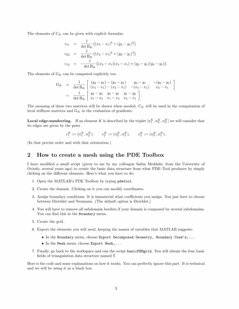
The elements of CK can be given with explicit formulas:

c11 =1

det BK

((x3 − x1)2 + (y3 − y1)2

)c22 =

1

det BK

((x2 − x1)2 + (y2 − y1)2

)c12 = − 1

det BK

((x2 − x1)(x3 − x1) + (y2 − y1)(y3 − y1)

).

The elements of GK can be computed explicitly too

GK =1

det BK

[(y2 − y1)− (y3 − y1) y3 − y1 −(y2 − y1)(x3 − x1)− (x2 − x1) −(x3 − x1) x2 − x1

]=

1

det BK

[y2 − y3 y3 − y1 y1 − y2

x3 − x2 x1 − x3 x2 − x1

].

The meaning of these two matrices will be shown when needed: CK will be used in the computation oflocal stiffness matrices and GK in the evaluation of gradients.

Local edge-numbering. If an element K is described by the triplet [nK1 , nK2 , n

K3 ] we will consider that

its edges are given by the pairs

eK1 := (nK1 , nK2 ), eK2 := (nK2 , n

K3 ), eK3 := (nK3 , n

K1 ).

(In that precise order and with that orientation.)

2 How to create a mesh using the PDE Toolbox

I have modified a small script (given to me by my colleague Salim Meddahi, from the University ofOviedo, several years ago) to create the basic data structure from what PDE–Tool produces by simplyclicking on the different elements. Here’s what you have to do:

1. Open the MATLAB’s PDE Toolbox by typing pdetool

2. Create the domain. Clicking on it you can modify coordinates.

3. Assign boundary conditions. It is immaterial what coefficients you assign. You just have to choosebetween Dirichlet and Neumann. (The default option is Dirichlet.)

4. You will have to remove all subdomain borders if your domain is composed by several subdomains.You can find this in the Boundary menu.

5. Create the grid.

6. Export the elements you will need, keeping the names of variables that MATLAB suggests:

• In the Boundary menu, choose Export Decomposed Geometry, Boundary Cond’s,...

• In the Mesh menu, choose Export Mesh,...

7. Finally, go back to the workspace and run the script basicFEMgrid. You will obtain the four basicfields of triangulation data structure named T.

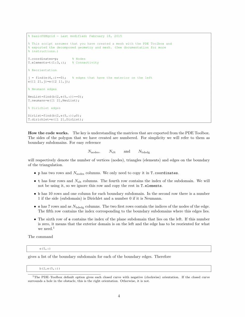
Here is the code and some explanations on how it works. You can perfectly ignore this part. It is technicaland we will be using it as a black box.

3

% basicFEMgrid − Last modified: February 18, 2015

% This script assumes that you have created a mesh with the PDE Toolbox and% exported the decomposed geometry and mesh. (See documentation for more% instructions.)

T.coordinates=p; % NodesT.elements=t(1:3,:); % Connectivity

% Reorientation

j = find(e(6,:)==0); % edges that have the exterior on the lefte([1 2],j)=e([2 1],j);

% Neumann edges

NeuList=find(b(2,e(5,:))==0);T.neumann=e([1 2],NeuList);

% Dirichlet edges

DirList=find(b(2,e(5,:))6=0);T.dirichlet=e([1 2],DirList);

How the code works. The key is understanding the matrices that are exported from the PDE Toolbox.The sides of the polygon that we have created are numbered. For simplicity we will refer to them asboundary subdomains. For easy reference

Nnodes, Nelt and Nbdedg

will respectively denote the number of vertices (nodes), triangles (elements) and edges on the boundaryof the triangulation.

• p has two rows and Nnodes columns. We only need to copy it in T.coordinates.

• t has four rows and Nelt columns. The fourth row contains the index of the subdomain. We willnot be using it, so we ignore this row and copy the rest in T.elements.

• b has 10 rows and one column for each boundary subdomain. In the second row there is a number1 if the side (subdomain) is Dirichlet and a number 0 if it is Neumann.

• e has 7 rows and as Nbdedg columns. The two first rows contain the indices of the nodes of the edge.The fifth row contains the index corresponding to the boundary subdomains where this edges lies.

• The sixth row of e contains the index of the plane subdomain that lies on the left. If this numberis zero, it means that the exterior domain is on the left and the edge has to be reoriented for whatwe need.1

The command

e(5,:)

gives a list of the boundary subdomain for each of the boundary edges. Therefore

b(2,e(5,:))

1The PDE–Toolbox default option gives each closed curve with negative (clockwise) orientation. If the closed curvesurrounds a hole in the obstacle, this is the right orientation. Otherwise, it is not.

4

is a list of ones and zeros: there is a one for edges on the Neumann boundary and a zero for edges on theDirichlet boundary. Finally,

NeuList=find(b(2,e(5,:))==0);DirList=find(b(2,e(5,:))6=0);

are the lists of Neumann and Dirichlet edges, constructed by looking at what positions of the vectorb(2,e(5,:)) there is a zero (Neumann) or a non–zero (Dirichlet). Once we know these lists, we candrop all other rows of e and separate what is left in the two lists T.dirichlet and T.neumann.

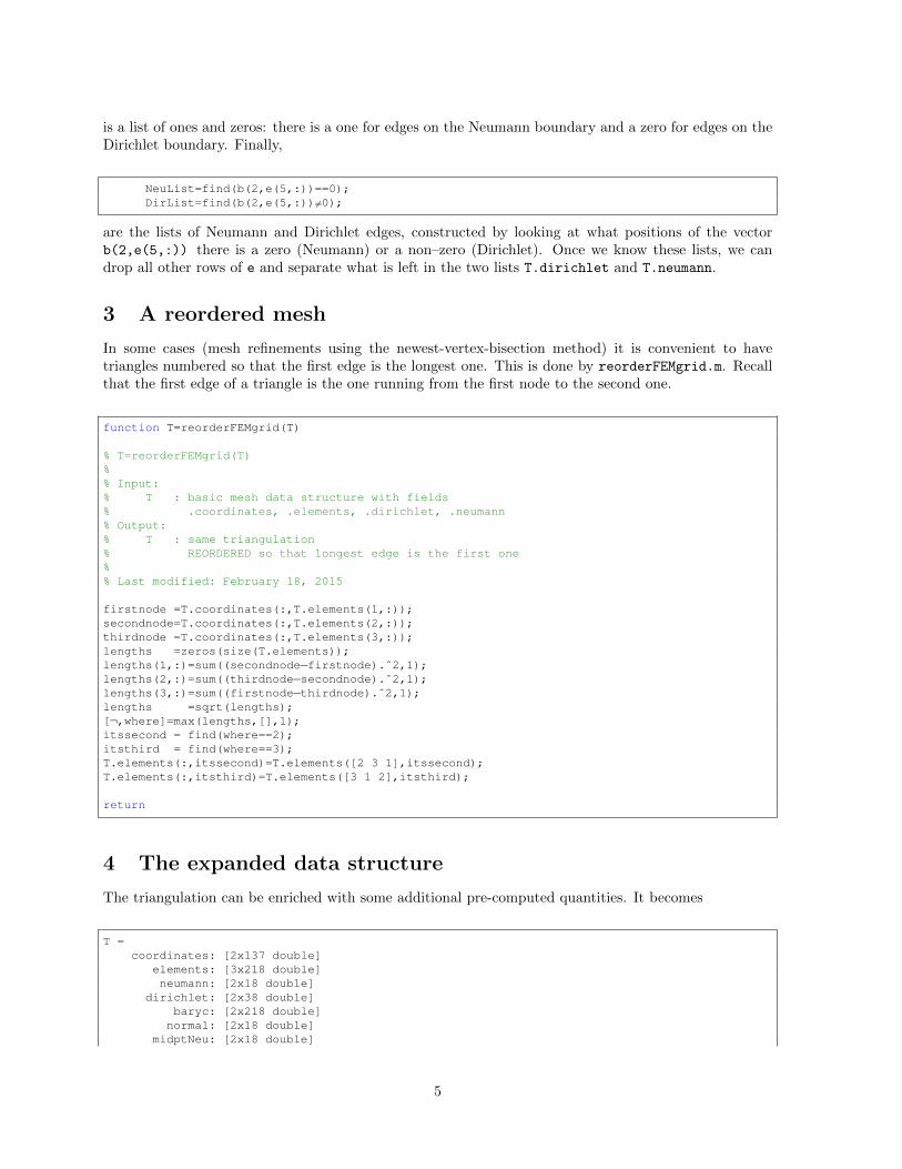
3 A reordered mesh

In some cases (mesh refinements using the newest-vertex-bisection method) it is convenient to havetriangles numbered so that the first edge is the longest one. This is done by reorderFEMgrid.m. Recallthat the first edge of a triangle is the one running from the first node to the second one.

function T=reorderFEMgrid(T)

% T=reorderFEMgrid(T)%% Input:% T : basic mesh data structure with fields% .coordinates, .elements, .dirichlet, .neumann% Output:% T : same triangulation% REORDERED so that longest edge is the first one%% Last modified: February 18, 2015

firstnode =T.coordinates(:,T.elements(1,:));secondnode=T.coordinates(:,T.elements(2,:));thirdnode =T.coordinates(:,T.elements(3,:));lengths =zeros(size(T.elements));lengths(1,:)=sum((secondnode−firstnode).ˆ2,1);lengths(2,:)=sum((thirdnode−secondnode).ˆ2,1);lengths(3,:)=sum((firstnode−thirdnode).ˆ2,1);lengths =sqrt(lengths);[¬,where]=max(lengths,[],1);itssecond = find(where==2);itsthird = find(where==3);T.elements(:,itssecond)=T.elements([2 3 1],itssecond);T.elements(:,itsthird)=T.elements([3 1 2],itsthird);

return

4 The expanded data structure

The triangulation can be enriched with some additional pre-computed quantities. It becomes

T =coordinates: [2x137 double]

elements: [3x218 double]neumann: [2x18 double]

dirichlet: [2x38 double]baryc: [2x218 double]normal: [2x18 double]

midptNeu: [2x18 double]

5

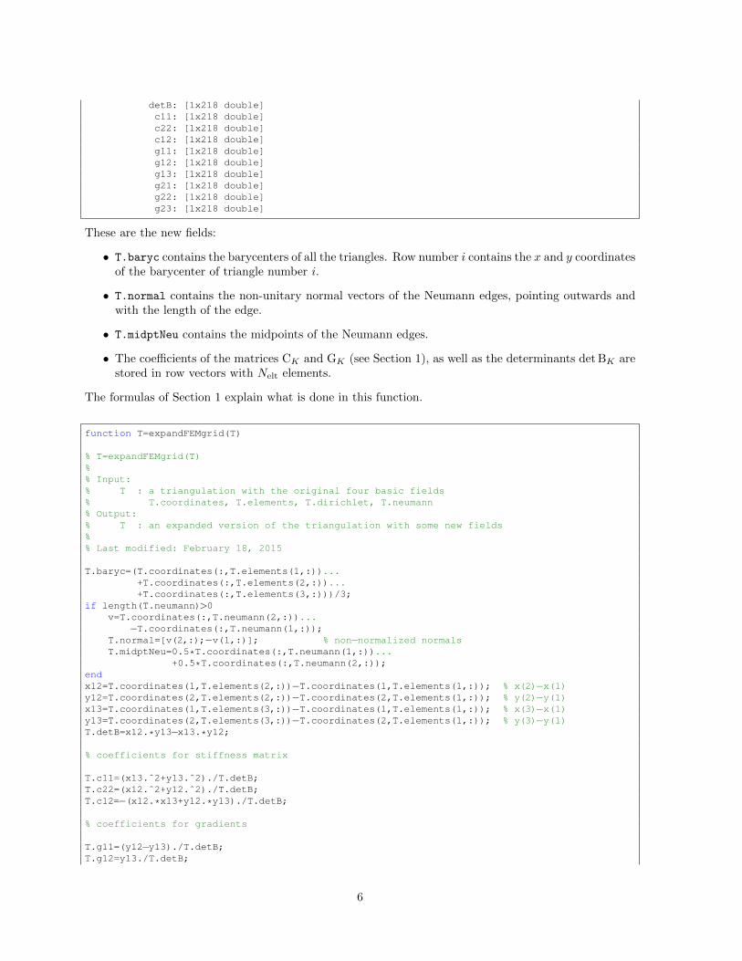
detB: [1x218 double]c11: [1x218 double]c22: [1x218 double]c12: [1x218 double]g11: [1x218 double]g12: [1x218 double]g13: [1x218 double]g21: [1x218 double]g22: [1x218 double]g23: [1x218 double]

These are the new fields:

• T.baryc contains the barycenters of all the triangles. Row number i contains the x and y coordinatesof the barycenter of triangle number i.

• T.normal contains the non-unitary normal vectors of the Neumann edges, pointing outwards andwith the length of the edge.

• T.midptNeu contains the midpoints of the Neumann edges.

• The coefficients of the matrices CK and GK (see Section 1), as well as the determinants det BK arestored in row vectors with Nelt elements.

The formulas of Section 1 explain what is done in this function.

function T=expandFEMgrid(T)

% T=expandFEMgrid(T)%% Input:% T : a triangulation with the original four basic fields% T.coordinates, T.elements, T.dirichlet, T.neumann% Output:% T : an expanded version of the triangulation with some new fields%% Last modified: February 18, 2015

T.baryc=(T.coordinates(:,T.elements(1,:))...+T.coordinates(:,T.elements(2,:))...+T.coordinates(:,T.elements(3,:)))/3;

if length(T.neumann)>0v=T.coordinates(:,T.neumann(2,:))...

−T.coordinates(:,T.neumann(1,:));T.normal=[v(2,:);−v(1,:)]; % non−normalized normalsT.midptNeu=0.5*T.coordinates(:,T.neumann(1,:))...

+0.5*T.coordinates(:,T.neumann(2,:));endx12=T.coordinates(1,T.elements(2,:))−T.coordinates(1,T.elements(1,:)); % x(2)−x(1)y12=T.coordinates(2,T.elements(2,:))−T.coordinates(2,T.elements(1,:)); % y(2)−y(1)x13=T.coordinates(1,T.elements(3,:))−T.coordinates(1,T.elements(1,:)); % x(3)−x(1)y13=T.coordinates(2,T.elements(3,:))−T.coordinates(2,T.elements(1,:)); % y(3)−y(1)T.detB=x12.*y13−x13.*y12;

% coefficients for stiffness matrix

T.c11=(x13.ˆ2+y13.ˆ2)./T.detB;T.c22=(x12.ˆ2+y12.ˆ2)./T.detB;T.c12=−(x12.*x13+y12.*y13)./T.detB;

% coefficients for gradients

T.g11=(y12−y13)./T.detB;T.g12=y13./T.detB;

6

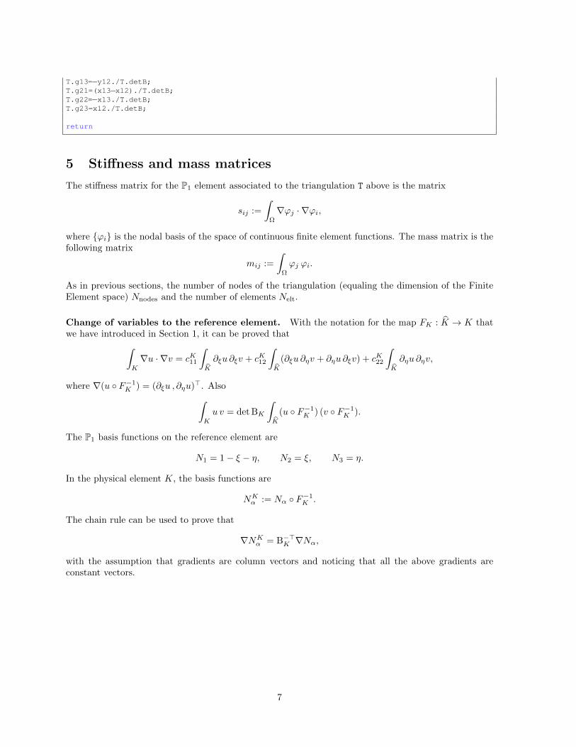
T.g13=−y12./T.detB;T.g21=(x13−x12)./T.detB;T.g22=−x13./T.detB;T.g23=x12./T.detB;

return

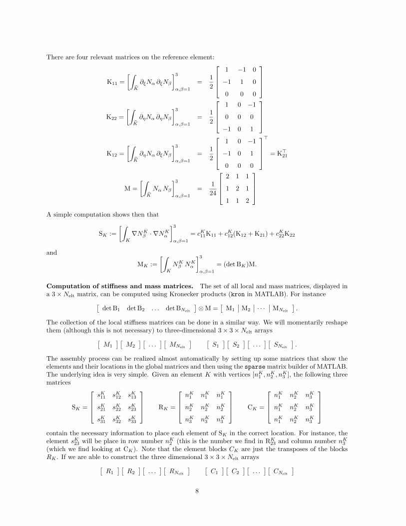
5 Stiffness and mass matrices

The stiffness matrix for the P1 element associated to the triangulation T above is the matrix

sij :=

∫Ω

∇ϕj · ∇ϕi,

where ϕi is the nodal basis of the space of continuous finite element functions. The mass matrix is thefollowing matrix

mij :=

∫Ω

ϕj ϕi.

As in previous sections, the number of nodes of the triangulation (equaling the dimension of the FiniteElement space) Nnodes and the number of elements Nelt.

Change of variables to the reference element. With the notation for the map FK : K → K thatwe have introduced in Section 1, it can be proved that∫

K

∇u · ∇v = cK11

∫K

∂ξu ∂ξv + cK12

∫K

(∂ξu ∂ηv + ∂ηu ∂ξv) + cK22

∫K

∂ηu ∂ηv,

where ∇(u F−1K ) = (∂ξu , ∂ηu)>. Also∫

K

u v = det BK

∫K

(u F−1K ) (v F−1

K ).

The P1 basis functions on the reference element are

N1 = 1− ξ − η, N2 = ξ, N3 = η.

In the physical element K, the basis functions are

NKα := Nα F−1

K .

The chain rule can be used to prove that

∇NKα = B−>K ∇Nα,

with the assumption that gradients are column vectors and noticing that all the above gradients areconstant vectors.

7

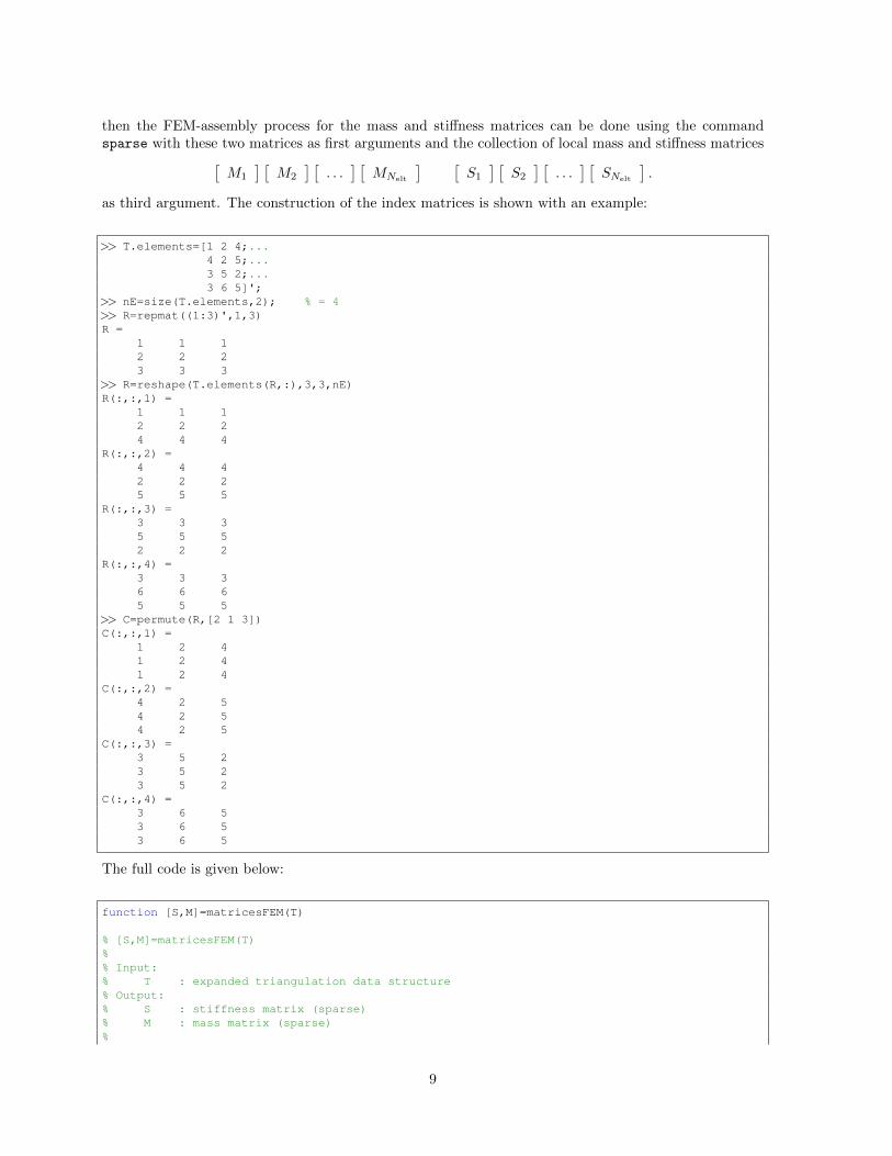
There are four relevant matrices on the reference element:

K11 =

[∫K

∂ξNα ∂ξNβ

]3

α,β=1

=1

2

1 −1 0

−1 1 0

0 0 0

K22 =

[∫K

∂ηNα ∂ηNβ

]3

α,β=1

=1

2

1 0 −1

0 0 0

−1 0 1

K12 =

[∫K

∂ηNα ∂ξNβ

]3

α,β=1

=1

2

1 0 −1

−1 0 1

0 0 0

>

= K>21

M =

[∫K

NαNβ

]3

α,β=1

=1

24

2 1 1

1 2 1

1 1 2

A simple computation shows then that

SK :=

[∫K

∇NKβ · ∇NK

α

]3

α,β=1

= cK11K11 + cK12(K12 + K21) + cK22K22

and

MK :=

[∫K

NKβ NK

α

]3

α,β=1

= (det BK)M.

Computation of stiffness and mass matrices. The set of all local and mass matrices, displayed ina 3×Nelt matrix, can be computed using Kronecker products (kron in MATLAB). For instance[

det B1 det B2 . . . det BNelt

]⊗M =

[M1 M2 · · · MNelt

].

The collection of the local stiffness matrices can be done in a similar way. We will momentarily reshapethem (although this is not necessary) to three-dimensional 3× 3×Nelt arrays[

M1

] [M2

] [. . .

] [MNelt

] [S1

] [S2

] [. . .

] [SNelt

].

The assembly process can be realized almost automatically by setting up some matrices that show theelements and their locations in the global matrices and then using the sparse matrix builder of MATLAB.The underlying idea is very simple. Given an element K with vertices [nK1 , n

K2 , n

K3 ], the following three

matrices

SK =

sK11 sK12 sK13

sK21 sK22 sK23

sK31 sK32 sK33

RK =

nK1 nK1 nK1

nK2 nK2 nK2

nK3 nK3 nK3

CK =

nK1 nK2 nK3

nK1 nK2 nK3

nK1 nK2 nK3

contain the necessary information to place each element of SK in the correct location. For instance, theelement sK23 will be place in row number nK2 (this is the number we find in RK

23 and column number nK3(which we find looking at CK). Note that the element blocks CK are just the transposes of the blocksRK . If we are able to construct the three dimensional 3× 3×Nelt arrays[

R1

] [R2

] [. . .

] [RNelt

] [C1

] [C2

] [. . .

] [CNelt

]8

then the FEM-assembly process for the mass and stiffness matrices can be done using the commandsparse with these two matrices as first arguments and the collection of local mass and stiffness matrices[

M1

] [M2

] [. . .

] [MNelt

] [S1

] [S2

] [. . .

] [SNelt

].

as third argument. The construction of the index matrices is shown with an example:

>> T.elements=[1 2 4;...4 2 5;...3 5 2;...3 6 5]';

>> nE=size(T.elements,2); % = 4>> R=repmat((1:3)',1,3)R =

1 1 12 2 23 3 3

>> R=reshape(T.elements(R,:),3,3,nE)R(:,:,1) =

1 1 12 2 24 4 4

R(:,:,2) =4 4 42 2 25 5 5

R(:,:,3) =3 3 35 5 52 2 2

R(:,:,4) =3 3 36 6 65 5 5

>> C=permute(R,[2 1 3])C(:,:,1) =

1 2 41 2 41 2 4

C(:,:,2) =4 2 54 2 54 2 5

C(:,:,3) =3 5 23 5 23 5 2

C(:,:,4) =3 6 53 6 53 6 5

The full code is given below:

function [S,M]=matricesFEM(T)

% [S,M]=matricesFEM(T)%% Input:% T : expanded triangulation data structure% Output:% S : stiffness matrix (sparse)% M : mass matrix (sparse)%

9

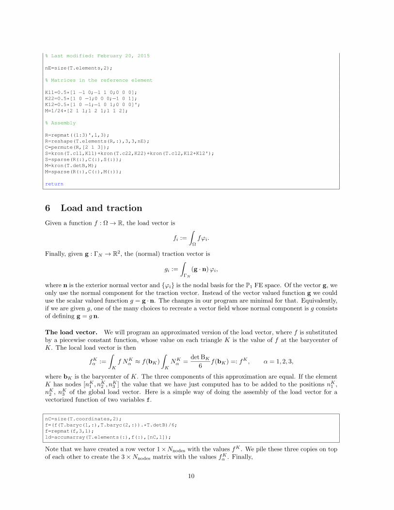
% Last modified: February 20, 2015

nE=size(T.elements,2);

% Matrices in the reference element

K11=0.5*[1 −1 0;−1 1 0;0 0 0];K22=0.5*[1 0 −1;0 0 0;−1 0 1];K12=0.5*[1 0 −1;−1 0 1;0 0 0]';M=1/24*[2 1 1;1 2 1;1 1 2];

% Assembly

R=repmat((1:3)',1,3);R=reshape(T.elements(R,:),3,3,nE);C=permute(R,[2 1 3]);S=kron(T.c11,K11)+kron(T.c22,K22)+kron(T.c12,K12+K12');S=sparse(R(:),C(:),S(:));M=kron(T.detB,M);M=sparse(R(:),C(:),M(:));

return

6 Load and traction

Given a function f : Ω→ R, the load vector is

fi :=

∫Ω

fϕi.

Finally, given g : ΓN → R2, the (normal) traction vector is

gi :=

∫ΓN

(g · n)ϕi,

where n is the exterior normal vector and ϕi is the nodal basis for the P1 FE space. Of the vector g, weonly use the normal component for the traction vector. Instead of the vector valued function g we coulduse the scalar valued function g = g ·n. The changes in our program are minimal for that. Equivalently,if we are given g, one of the many choices to recreate a vector field whose normal component is g consistsof defining g = g n.

The load vector. We will program an approximated version of the load vector, where f is substitutedby a piecewise constant function, whose value on each triangle K is the value of f at the barycenter ofK. The local load vector is then

fKα :=

∫K

f NKα ≈ f(bK)

∫K

NKα =

det BK6

f(bK) =: fK , α = 1, 2, 3,

where bK is the barycenter of K. The three components of this approximation are equal. If the elementK has nodes [nK1 , n

K2 , n

K3 ] the value that we have just computed has to be added to the positions nK1 ,

nK2 , nK3 of the global load vector. Here is a simple way of doing the assembly of the load vector for avectorized function of two variables f.

nC=size(T.coordinates,2);f=(f(T.baryc(1,:),T.baryc(2,:)).*T.detB)/6;f=repmat(f,3,1);ld=accumarray(T.elements(:),f(:),[nC,1]);

Note that we have created a row vector 1×Nnodes with the values fK . We pile these three copies on topof each other to create the 3×Nnodes matrix with the values fKα . Finally,

10

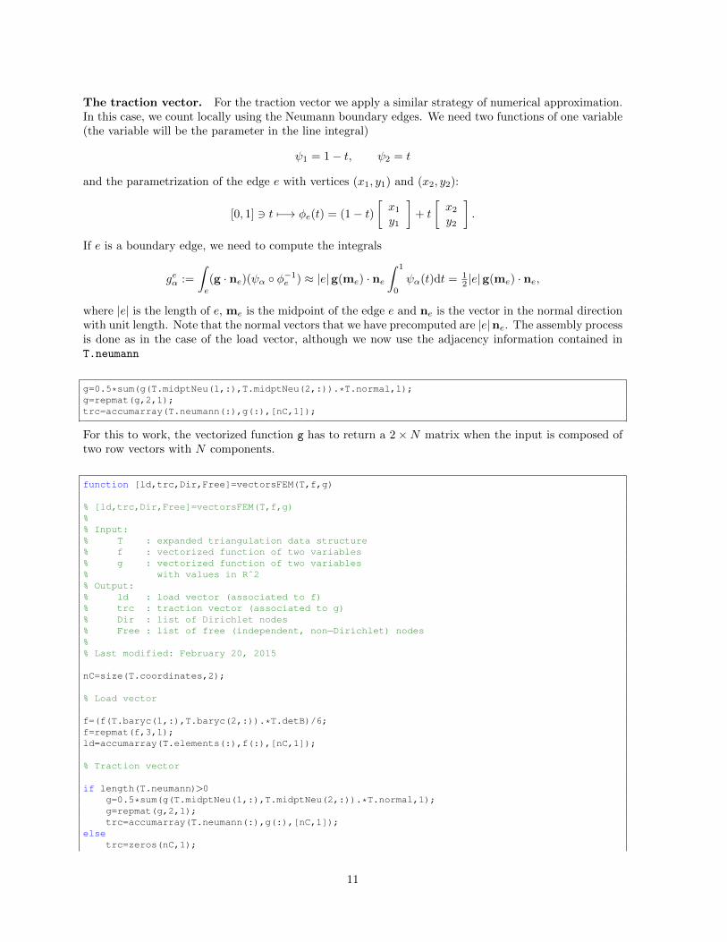
The traction vector. For the traction vector we apply a similar strategy of numerical approximation.In this case, we count locally using the Neumann boundary edges. We need two functions of one variable(the variable will be the parameter in the line integral)

ψ1 = 1− t, ψ2 = t

and the parametrization of the edge e with vertices (x1, y1) and (x2, y2):

[0, 1] 3 t 7−→ φe(t) = (1− t)[x1

y1

]+ t

[x2

y2

].

If e is a boundary edge, we need to compute the integrals

geα :=

∫e

(g · ne)(ψα φ−1e ) ≈ |e|g(me) · ne

∫ 1

0

ψα(t)dt = 12 |e|g(me) · ne,

where |e| is the length of e, me is the midpoint of the edge e and ne is the vector in the normal directionwith unit length. Note that the normal vectors that we have precomputed are |e|ne. The assembly processis done as in the case of the load vector, although we now use the adjacency information contained inT.neumann

g=0.5*sum(g(T.midptNeu(1,:),T.midptNeu(2,:)).*T.normal,1);g=repmat(g,2,1);trc=accumarray(T.neumann(:),g(:),[nC,1]);

For this to work, the vectorized function g has to return a 2×N matrix when the input is composed oftwo row vectors with N components.

function [ld,trc,Dir,Free]=vectorsFEM(T,f,g)

% [ld,trc,Dir,Free]=vectorsFEM(T,f,g)%% Input:% T : expanded triangulation data structure% f : vectorized function of two variables% g : vectorized function of two variables% with values in Rˆ2% Output:% ld : load vector (associated to f)% trc : traction vector (associated to g)% Dir : list of Dirichlet nodes% Free : list of free (independent, non−Dirichlet) nodes%% Last modified: February 20, 2015

nC=size(T.coordinates,2);

% Load vector

f=(f(T.baryc(1,:),T.baryc(2,:)).*T.detB)/6;f=repmat(f,3,1);ld=accumarray(T.elements(:),f(:),[nC,1]);

% Traction vector

if length(T.neumann)>0g=0.5*sum(g(T.midptNeu(1,:),T.midptNeu(2,:)).*T.normal,1);g=repmat(g,2,1);trc=accumarray(T.neumann(:),g(:),[nC,1]);

elsetrc=zeros(nC,1);

11

end

% Dir and Free nodes

Dir=unique(T.dirichlet);Free=(1:nC)'; Free(Dir)=[];

return

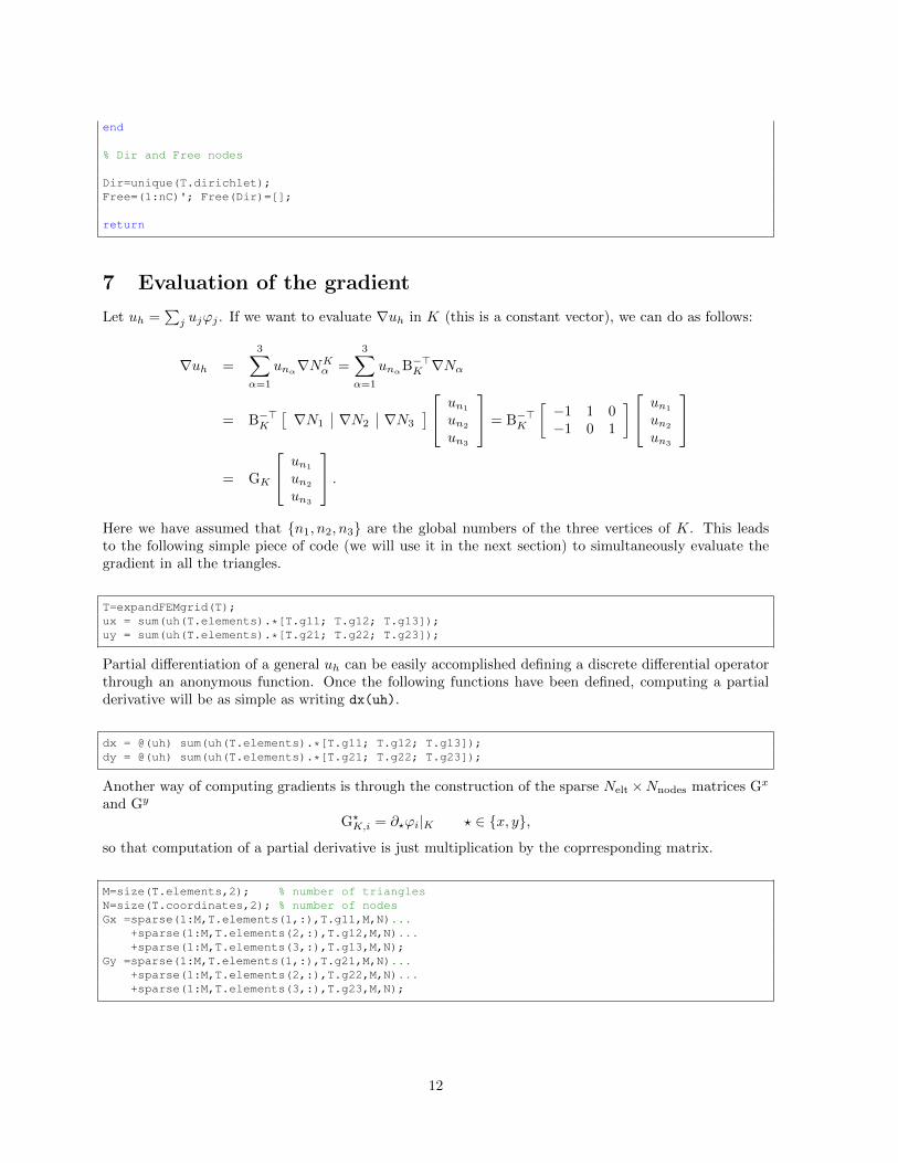
7 Evaluation of the gradient

Let uh =∑j ujϕj . If we want to evaluate ∇uh in K (this is a constant vector), we can do as follows:

∇uh =

3∑α=1

unα∇NKα =

3∑α=1

unαB−>K ∇Nα

= B−>K[∇N1 ∇N2 ∇N3

] un1

un2

un3

= B−>K

[−1 1 0−1 0 1

] un1

un2

un3

= GK

un1

un2

un3

.Here we have assumed that n1, n2, n3 are the global numbers of the three vertices of K. This leadsto the following simple piece of code (we will use it in the next section) to simultaneously evaluate thegradient in all the triangles.

T=expandFEMgrid(T);ux = sum(uh(T.elements).*[T.g11; T.g12; T.g13]);uy = sum(uh(T.elements).*[T.g21; T.g22; T.g23]);

Partial differentiation of a general uh can be easily accomplished defining a discrete differential operatorthrough an anonymous function. Once the following functions have been defined, computing a partialderivative will be as simple as writing dx(uh).

dx = @(uh) sum(uh(T.elements).*[T.g11; T.g12; T.g13]);dy = @(uh) sum(uh(T.elements).*[T.g21; T.g22; T.g23]);

Another way of computing gradients is through the construction of the sparse Nelt×Nnodes matrices Gx

and Gy

G?K,i = ∂?ϕi|K ? ∈ x, y,

so that computation of a partial derivative is just multiplication by the coprresponding matrix.

M=size(T.elements,2); % number of trianglesN=size(T.coordinates,2); % number of nodesGx =sparse(1:M,T.elements(1,:),T.g11,M,N)...

+sparse(1:M,T.elements(2,:),T.g12,M,N)...+sparse(1:M,T.elements(3,:),T.g13,M,N);

Gy =sparse(1:M,T.elements(1,:),T.g21,M,N)...+sparse(1:M,T.elements(2,:),T.g22,M,N)...+sparse(1:M,T.elements(3,:),T.g23,M,N);

12

8 L2 and H1 errors

The aim of the following piece of code is the approximation of(∫Ω

|uh − u|2)1/2

and

(∫Ω

|∇uh −∇u|2)1/2

where uh is a discrete function on the triangulation and both u and ∇u = (ux, uy)> can be computed bymeans of vectorized functions.

A basic quadrature rule on K. We assume that we have a formula to approximate integrals on K:

∫K

f ≈Nquad∑`=1

ω` f(ξ`, η`).

With this formula, we can approximate∫K

u = det BK

∫K

u FK ≈ det BK∑`

ω` u(FK(ξ`, η`)︸ ︷︷ ︸=:(xK` ,y

K` )

).

We therefore have to address two relatively simple problems:

• The computation of (xK` , yK` ).

• The evaluation of uh in these points.

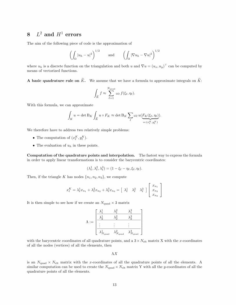
Computation of the quadrature points and interpolation. The fastest way to express the formulain order to apply linear transformations is to consider the barycentric coordinates:

(λ1` , λ

2` , λ

3`) = (1− ξ` − η`, ξ`, η`).

Then, if the triangle K has nodes n1, n2, n3, we compute

xK` = λ1`xn1

+ λ2`xn2

+ λ3`xn3

=[λ1` λ2

` λ3`

] xn1

xn2

xn3

It is then simple to see how if we create an Nquad × 3 matrix

Λ :=

λ1

1 λ21 λ3

1

λ12 λ2

2 λ32

......

...

λ1Nquad

λ2Nquad

λ3Nquad

with the barycentric coordinates of all quadrature points, and a 3×Nelt matrix X with the x-coordinatesof all the nodes (vertices) of all the elements, then

ΛX

is an Nquad × Nelt matrix with the x-coordinates of all the quadrature points of all the elements. Asimilar computation can be used to create the Nquad×Nelt matrix Y with all the y-coordinates of all thequadrature points of all the elements.

13

The evaluation of uh at the quadrature points is just linear interpolation of the values of uh at the vertices.Therefore

uh(xK` , yK` ) = un1

λ1` + un2

λ2` + un3

λ3` =

[λ1` λ2

` λ3`

] un1

un2

un3

The computation of the values of uh in all quadrature points of all the elements can be done exactly asthe computation of the coordinates of these points.

Computation of the L2-error. We just need to compute∑K

det BK

(∑`

ω` |uh(xK` , yK` )− u(xK` , y

K` )|2

).

This can be done in three steps that we will group in the program:

(a) Compute the errors in each of the quadrature points

eK` := |uh(xK` , yK` )− u(xK` , y

K` )|2,

storing the result in an Nquad ×Nelt matrix.

(b) Compute the errors on each of the elements (still not corrected by the Jacobians)

eK :=[ω1 . . . ωNquad

] eK1...

eKNquad

(c) Add the contribution of each of the elements, correcting with the Jacobian∑

K

det BK eK .

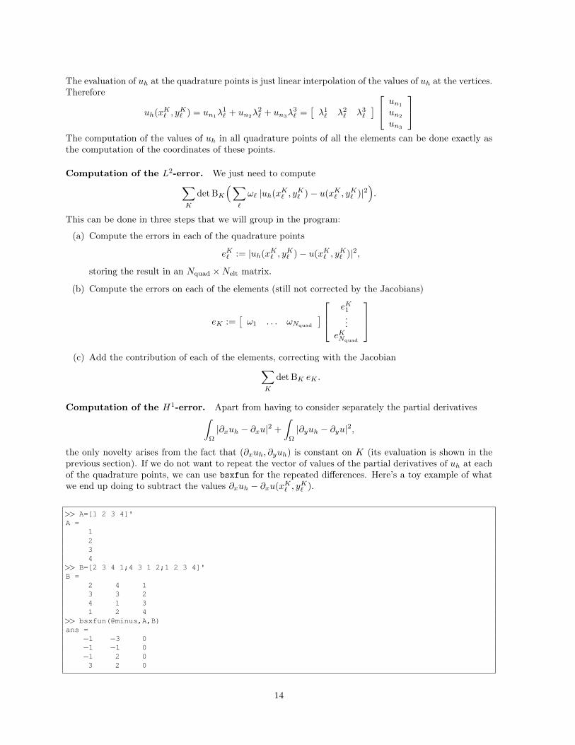
Computation of the H1-error. Apart from having to consider separately the partial derivatives∫Ω

|∂xuh − ∂xu|2 +

∫Ω

|∂yuh − ∂yu|2,

the only novelty arises from the fact that (∂xuh, ∂yuh) is constant on K (its evaluation is shown in theprevious section). If we do not want to repeat the vector of values of the partial derivatives of uh at eachof the quadrature points, we can use bsxfun for the repeated differences. Here’s a toy example of whatwe end up doing to subtract the values ∂xuh − ∂xu(xK` , y

K` ).

>> A=[1 2 3 4]'A =

1234

>> B=[2 3 4 1;4 3 1 2;1 2 3 4]'B =

2 4 13 3 24 1 31 2 4

>> bsxfun(@minus,A,B)ans =

−1 −3 0−1 −1 0−1 2 03 2 0

14

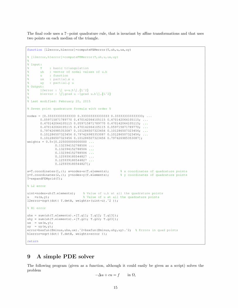
The final code uses a 7−point quadrature rule, that is invariant by affine transformations and that usestwo points on each median of the triangle.

function [l2error,h1error]=computeFEMerror(T,uh,u,ux,uy)

% [l2error,h1error]=computeFEMerror(T,uh,u,ux,uy)%% Input:% T : basic triangulation% uh : vector of nodal values of u h% u : function% ux : partial x u% uy : partial y u% Output:% l2error : \ | u−u h \ | Lˆ2% h1error : \|\grad u −\grad u h \ | Lˆ2%% Last modified: February 20, 2015

% Seven point quadrature formula with order 5

nodes = [0.333333333333333 0.333333333333333 0.333333333333333; ...0.059715871789770 0.470142064105115 0.470142064105115; ...0.470142064105115 0.059715871789770 0.470142064105115; ...0.470142064105115 0.470142064105115 0.059715871789770; ...0.797426985353087 0.101286507323456 0.101286507323456; ...0.101286507323456 0.797426985353087 0.101286507323456; ...0.101286507323456 0.101286507323456 0.797426985353087];

weights = 0.5*[0.225000000000000 ...0.132394152788506 ...0.132394152788506 ...0.132394152788506 ...0.125939180544827 ...0.125939180544827 ...0.125939180544827];

x=T.coordinates(1,:); x=nodes*x(T.elements); % x coordinates of quadrature pointsy=T.coordinates(2,:); y=nodes*y(T.elements); % y coordinates of quadrature pointsT=expandFEMgrid(T);

% L2 error

uint=nodes*uh(T.elements); % Value of u h at all the quadrature pointsu =u(x,y); % Value of u at all the quadrature pointsl2error=sqrt(dot( T.detB, weights*(uint−u).ˆ2 ));

% H1 error

uhx = sum(uh(T.elements).*[T.g11; T.g12; T.g13]);uhy = sum(uh(T.elements).*[T.g21; T.g22; T.g23]);ux = ux(x,y);uy = uy(x,y);error=bsxfun(@minus,uhx,ux).ˆ2+bsxfun(@minus,uhy,uy).ˆ2; % Errors in quad pointsh1error=sqrt(dot( T.detB, weights*error ));

return

9 A simple PDE solver

The following program (given as a function, although it could easily be given as a script) solves theproblem

−∆u+ cu = f in Ω,

15

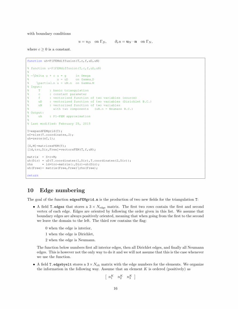
with boundary conditions

u = uD on ΓD, ∂νu = uN · n on ΓN ,

where c ≥ 0 is a constant.

function uh=P1FEMdiffusion(T,c,f,uD,uN)

% function u=P1FEMdiffusion(T,c,f,uD,uN)%% −\Delta u + c u = g in Omega% u = uD on Gamma D% \partial n u = uN.n on Gamma N% Input:% T : basic triangulation% c : constant parameter% f : vectorized function of two variables (source)% uD : vectorized function of two variables (Dirichlet B.C.)% uN : vectorized function of two variables% with two components (uN.n = Neumann B.C.)% Output:% uh : P1−FEM approximation%% Last modified: February 25, 2015

T=expandFEMgrid(T);nC=size(T.coordinates,2);uh=zeros(nC,1);

[S,M]=matricesFEM(T);[ld,trc,Dir,Free]=vectorsFEM(T,f,uN);

matrix = S+c*M;uh(Dir) = uD(T.coordinates(1,Dir),T.coordinates(2,Dir));rhs = ld+trc−matrix(:,Dir)*uh(Dir);uh(Free)= matrix(Free,Free)\rhs(Free);

return

10 Edge numbering

The goal of the function edgesFEMgrid.m is the production of two new fields for the triangulation T:

• A field T.edges that stores a 3 × Nedge matrix. The first two rows contain the first and secondvertex of each edge. Edges are oriented by following the order given in this list. We assume thatboundary edges are always positively oriented, meaning that when going from the first to the secondwe leave the domain to the left. The third row contains the flag:

0 when the edge is interior,

1 when the edge is Dirichlet,

2 when the edge is Neumann.

The function below numbers first all interior edges, then all Dirichlet edges, and finally all Neumannedges. This is however not the only way to do it and we will not assume that this is the case wheneverwe use the function.

• A field T.edgebyelt stores a 3×Nelt matrix with the edge numbers for the elements. We organizethe information in the following way. Assume that an element K is ordered (positively) as[

nK1 nK2 nK3]

16

We next look for the edges

eK1 = [nK1 , nK2 ], eK2 = [nK2 , n

K2 ], eK3 = [nK3 , n

K1 ]

in the global list of edges. If eK1 = ej (j ∈ 1, . . . , Nedge), we store the number j in the first rowand K-th column. If [nK2 , n

K1 ] = ej (that is, we find the edge reversed in the global list), we store

the number j − 1 instead. This is done for the second and third edge as well. Therefore the K-thcolumn of T.edgebyelt contains the global reference of the local edges (from first node to second,second to third, and third to first) and the orientation as the sign of the entry.

This is the structure of this function. The way it is programmed, it uses several sparse matrices to keepconnectivity information.

1. Create a sparse matrix edges with the pairs (nK1 , nK2 ), (nK2 , n

K3 ), (nK3 , n

K1 ), storing the number one

in each entry. Since all elements are positively oriented, if the pairs (i, j) and (j, i) are marked inthe matrix, it is beacuse the edge is interior. Boundary edges do not appear in symmetric locationsof the matrix.

2. We then delete the boundary edges and keep only the upper triangular part of the remainingmatrices. At this moment we can count the number of interior edges: Nint−edg. We already knewthe number of Dirichlet and Neumann edges.

3. The list T.edges is composed of the pairs (i, j) such that edges(i, j) = 1, followed by T.dirichlet

and T.neumann.

4. At the same time that we create the list T.edges we modify the matrix in the following way:

• In the locations where edges is non-zero, we place the numbers 1, . . . , Nint−edge in the sameorder that we placed these pairs in the list of edges. We the write edges=edges-edges’ toplace negative values in the locations of reversed edges.

• We place the numbers Nint−edge + 1, Ndir +Nint−edge on the locations of Dirichlet edges.

• We place the numbers Nint−edge +Ndir + 1, Nint−edge +Ndir +Nneu on the locations of theNeumann edges.

5. The final step consists of going element by element and locating the pairs

(nK1 , nK2 ), (n2,

K , nK3 ), (nK3 , nK1 )

in the matrix edges. These are the columns of T.edgebyelt. Note that this can be done in aneasy way using the function sub2ind. Basically, if rows and cols are lists of the same length

A(sub2ind([N, N], rows, cols))

gives the entries of the matrix A that are located in the positions

(rows(i), cols(i)).

Since we are reading from a sparse matrix, we need to transform the output to a full matrix.

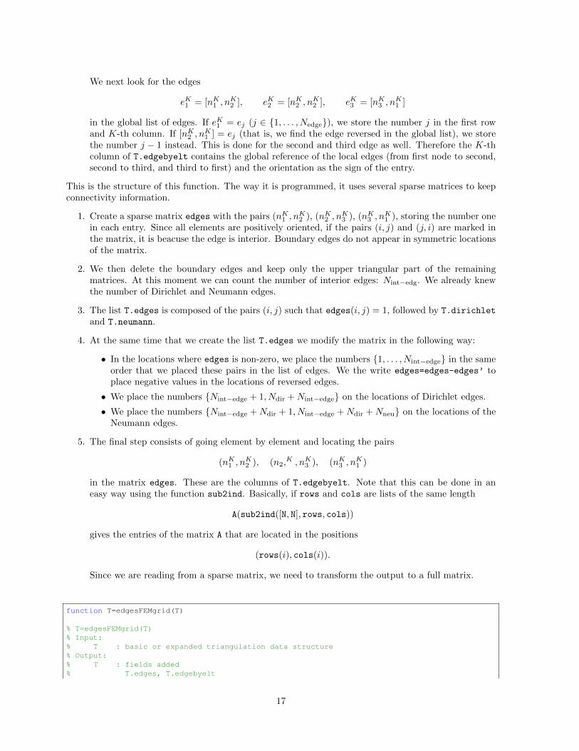
function T=edgesFEMgrid(T)

% T=edgesFEMgrid(T)% Input:% T : basic or expanded triangulation data structure% Output:% T : fields added% T.edges, T.edgebyelt

17

%% Last modified: February 25, 2015

N=size(T.coordinates,2);Ndir = size(T.dirichlet,2);Nneu = size(T.neumann,2);

edges = sparse(T.elements,T.elements([2 3 1],:),1); % all edgesedges = edges+edges';edges(find(edges==1))=0; % eliminate bd edges[i,j] = find(edges);Nint = sum(i<j);edges = sparse(i,j,i<j); % lower triangular

listInt=1:Nint;listDir=1+Nint:Nint+Ndir;listNeu=1+Nint+Ndir:Nint+Ndir+Nneu;

T.edges=[];if Nint>0

[i,j]=find(edges);T.edges=[T.edges [i'; j'; zeros(1,Nint)]];edges=sparse(i,j,listInt,N,N);edges=edges−edges';

endif Ndir>0

T.edges=[T.edges [T.dirichlet ; ones(1,Ndir)]];edges=edges+...

sparse(T.dirichlet(1,:),T.dirichlet(2,:),listDir,N,N);endif Nneu>0

T.edges=[T.edges [T.neumann; 2*ones(1,Nneu)]];edges=edges+...

sparse(T.neumann(1,:),T.neumann(2,:),listNeu,N,N);endT.edgebyelt=...

[full(edges(sub2ind([N,N],T.elements(1,:),T.elements(2,:))));...full(edges(sub2ind([N,N],T.elements(2,:),T.elements(3,:))));...full(edges(sub2ind([N,N],T.elements(3,:),T.elements(1,:))))];

return

11 Uniform (red) refinement of a triangulation

In a uniform red refinement, every triangle is subdivided into four equally shaped and sized triangles byjoining the midpoints of the edges. This is the gist of the process:

• We start by creating the lists T.edges and T.edgebyelt using edgesFEMgrid.m.

• Next, we add Nnodes to the edge number of each of the edges and assign the vertex number Nnodes+kto the edge number k. This gives a global numbering of all old and new nodes, keeping the oldnodes at the beginning of the list. Coordinates can be easily computed at this stage.

• Finally, we can refine the triangulation. If a triangle has vertices (n1, n2, n3) and midpoints(n4, n5, n6) (n4 is the midpoint of n1 and n2; n5 that of n2 and n3; n6 that of n3 and n1), the newtriangles are

(n1, n4, n6) (n2, n5, n4) (n3, n6, n5) (n4, n5, n6).

function T=refineFEMgridRed(T)

18

% T=refineFEMgridRed(T)%% Input:% T : basic triangulation% Output:% T : red refinement of T (basic triangulation data struct)%% Last modified: March 2, 2015

T=edgesFEMgrid(T);nC=size(T.coordinates,2);nElt=size(T.elements,2);

% Renumbering edges & constructing new mesh

midpoints=0.5*(T.coordinates(:,T.edges(1,:))+...T.coordinates(:,T.edges(2,:)));

T.coordinates=[T.coordinates midpoints];local = [T.elements; nC+abs(T.edgebyelt)];local = local([1 4 6 2 5 4 3 6 5 4 5 6],:);T.elements=reshape(local,3,4*nElt);

% Dirichlet and Neumann edges

if size(T.dirichlet,2)local = [T.dirichlet; nC+find(T.edges(3,:)==1)];T.dirichlet=[local([1 3],:) local([3 2],:)];

endif size(T.neumann,2)

local = [T.neumann; nC+find(T.edges(3,:)==2)];T.neumann=[local([1 3],:) local([3 2],:)];

end

T=rmfield(T,'edges','edgebyelt');

return

12 Newest Vertex Bisection

function T=refineFEMgridNVB(T,marked)

% T=refineFEMgridNVB(T,marked)%% Input:% T : triangulation in basic form (no need for longest edge at% beginning)% marked : list of marked elements% Output:% T : newest vertex bisection refined triangulation%% Mostly direct adaptation of code by Funken, Praetorious & Wissgott%% Last modified: March 9, 2015

T=reorderFEMgrid(T);T=edgesFEMgrid(T);T.edgebyelt=abs(T.edgebyelt);

nElt = size(T.elements,2);nEd = size(T.edges,2);nC = size(T.coordinates,2);nDir = size(T.dirichlet,2);

19

nNeu = size(T.neumann,2);

T.diredge = find(T.edges(3,:)==1);T.neuedge = find(T.edges(3,:)==2);

% Mark edges: at the end of this search we have a list of all marked Edges% that will welcome a node. Every triangle has either its first (longest)% edge marked (and possible more) or none at all.

markEdge = zeros(1,nEd);markEdge(T.edgebyelt(:,marked)) = 1;checknew = 1;while checknew

markElt = markEdge(T.edgebyelt);newElts = find( ¬markElt(1,:) & (markElt(2,:) | markElt(3,:)) );markEdge(T.edgebyelt(1,newElts)) = 1;checknew=length(newElts); % 6=0 if there are new edges

endidx = find(markEdge);nNewN = sum(markEdge(:));markEdge(idx) = nC + (1:nNewN);midpoints = (T.coordinates(:,T.edges(1,idx))...

+T.coordinates(:,T.edges(2,idx)))/2;T.coordinates=[T.coordinates midpoints];

if nDirrefDir = markEdge(T.diredge); % 0s or numbersmarkedEdges = find(refDir);if ¬isempty(markedEdges)

T.dirichlet = [T.dirichlet(:,¬refDir), ...[T.dirichlet(1,markedEdges);refDir(markedEdges)],...[refDir(markedEdges);T.dirichlet(2,markedEdges)]];

endend

if nNeurefNeu = markEdge(T.neuedge);markedEdges = find(refNeu);if ¬isempty(markedEdges)

T.neumann = [T.neumann(:,¬refNeu), ...[T.neumann(1,markedEdges);refNeu(markedEdges)],...[refNeu(markedEdges);T.neumann(2,markedEdges)]];

endend

% New nodes for refinement of elements: newNodes contains a zero when an% edge does not provide a new node and the number of node when it does% It is 3 x nElt

newNodes = markEdge(T.edgebyelt);

% Determine type of refinement for each element

markedEdges=sign(newNodes);first = markedEdges(1,:);second = markedEdges(2,:);third = markedEdges(3,:);

none = ¬first;bisec1 = first & ¬second & ¬third;bisec12 = first & second & ¬third;bisec13 = first & ¬second & third;all = first & second & third;

T.elements = [T.elements(:,none),...[T.elements(3,bisec1);T.elements(1,bisec1);newNodes(1,bisec1)],...

20

[T.elements(2,bisec1);T.elements(3,bisec1);newNodes(1,bisec1)],...[T.elements(3,bisec12);T.elements(1,bisec12);newNodes(1,bisec12)],...[newNodes(1,bisec12);T.elements(2,bisec12);newNodes(2,bisec12)],...[T.elements(3,bisec12);newNodes(1,bisec12);newNodes(2,bisec12)],...[newNodes(1,bisec13);T.elements(3,bisec13);newNodes(3,bisec13)],...[T.elements(1,bisec13);newNodes(1,bisec13);newNodes(3,bisec13)],...[T.elements(2,bisec13);T.elements(3,bisec13);newNodes(1,bisec13)],...[newNodes(1,all);T.elements(3,all);newNodes(3,all)],...[T.elements(1,all);newNodes(1,all);newNodes(3,all)],...[newNodes(1,all);T.elements(2,all);newNodes(2,all)],...[T.elements(3,all);newNodes(1,all);newNodes(2,all)]];

return

13 Variable coefficients and boundary mass

Pieces of the stiffness matrix. We want to compute the local matrices∫K

kij ∂jNKα ∂iN

Kβ , α, β ∈ 1, 2, 3, K ∈ Th, i, j ∈ 1, 2 ≡ x, y,

for given vectorized functions of two variables kij . We will only compute the pairs (1, 1), (2, 2), and (1, 2).Approximating the variable coefficient kij by its value at the barycenter we can proceed as follows:∫

K

kij∂jNKα ∂iN

Kβ ≈ kij(bK)

∫K

(e>j ∇NKα ) · (e>i ∇NK

β )

= kij(bK) det BK

∫K

(e>j B−>K ∇Nα) · (e>i B−>K ∇Nβ)

=

∫K

(DijK∇Nα) · ∇Nβ

where

DijK := kij(bK) det BK(B−1

K ei)(B−1K ej)

> =kij(bK)

det BKdK,id

>K,j .

In the last expression, dK,i are the columns of

(det BK) B−1K =

[y3 − y1 −(x3 − x1)−(y2 − y1) x2 − x1

],

and vKi = (xKi , yKi ) are the three vertices of K. Shortening

x21 = x2 − x1, x31 = x3 − x1, y21 = y2 − y1, y31 = y3 − y1,

we can expand

D11K =

k11(bK)

det BK

[y2

13 −y12y13

−y12y13 y212

],

D22K =

k22(bK)

det BK

[x2

13 −x12x13

−x12x13 x212

],

D12K =

k12(bK)

det BK

[−y13x13 x12y13

y12x13 −x12y12

].

Note finally that everything can be written in terms of the elements of the matrices DijK[∫

K

(DijK∇Nα) · ∇Nβ

]α,β

= dijK,11K11 + dijK,12K12 + dijK,21K21 + dijK,22K22,

which leads to Kronecker product computations (see Section 5). The assembly process is done with thesame strategies as the mass and stiffness matrices.

21

Variable mass matrix. Using the same kind of ideas, it is easy to compute∫K

cNKα N

Kβ ≈ c(bK) det BKMαβ

(see Section 5.)

Boundary mass matrix. A final matrix we will compute is∫ΓN

k ϕiϕj , i, j = 1, . . . , Nnodes,

where k is a function. Using the parametrized one-dimensional basis functions of Section 6, ψ1 = 1 − t,ψ2 = t, and the parametrization φe : [0, 1]→ e, we compute∫

e

k (ψαφ−1e )(ψβ φ−1

e ) ≈ |e|k(me)

∫ 1

0

ψα(t)ψβ(t)dt, α, β = 1, 2.

The matrix in the reference interval is

B =1

6

[2 11 2

]and, therefore, the local matrices are

|e|k(me)B.

These matrices can be computed using a Kronecker product. The assembly is done using the informationof T.dirichlet and T.neumann. The process is very similar to the one used for assembling the mass andstiffness matrix, substituting the list T.elements by the joint list of all boundary edges [T.dirichlet

T.neumann].

function [Sxx,Sxy,Syy,M,MB]=matricesFEMenhanced(T,kxx,kxy,kyy,c,k)

% [Sxx,Sxy,Syy,M,MB]=matricesFEMenhanced(T,kxx,kxy,kyy,c,k)%% Input:% T : expanded triangulation data structure% kxx, kxy, kyy, c, k : vectorized functions of two variables% Output:% Sxx, Sxy, Syy : variable stiffness matrices (sparse)% Sab = \int kab \partial b\phi i \partial a\phi j% M : variable mass matrix (sparse)% \int c \phi i \phi j% MB : boundary variable mass matrix (sparse)% \int \Gamma N k \phi i \phi j% Last modified: March 9, 2015

nE=size(T.elements,2);nC=size(T.coordinates,2);

% Matrices in the reference element

K11=0.5*[1 −1 0;−1 1 0;0 0 0];K22=0.5*[1 0 −1;0 0 0;−1 0 1];K12=0.5*[1 0 −1;−1 0 1;0 0 0]';M =1/24*[2 1 1;1 2 1;1 1 2];MB =1/6*[2 1;1 2];

% Evaluations of coefficients in barycenters

x=T.baryc(1,:); y=T.baryc(2,:);kxx=kxx(x,y)./T.detB;kyy=kyy(x,y)./T.detB;

22

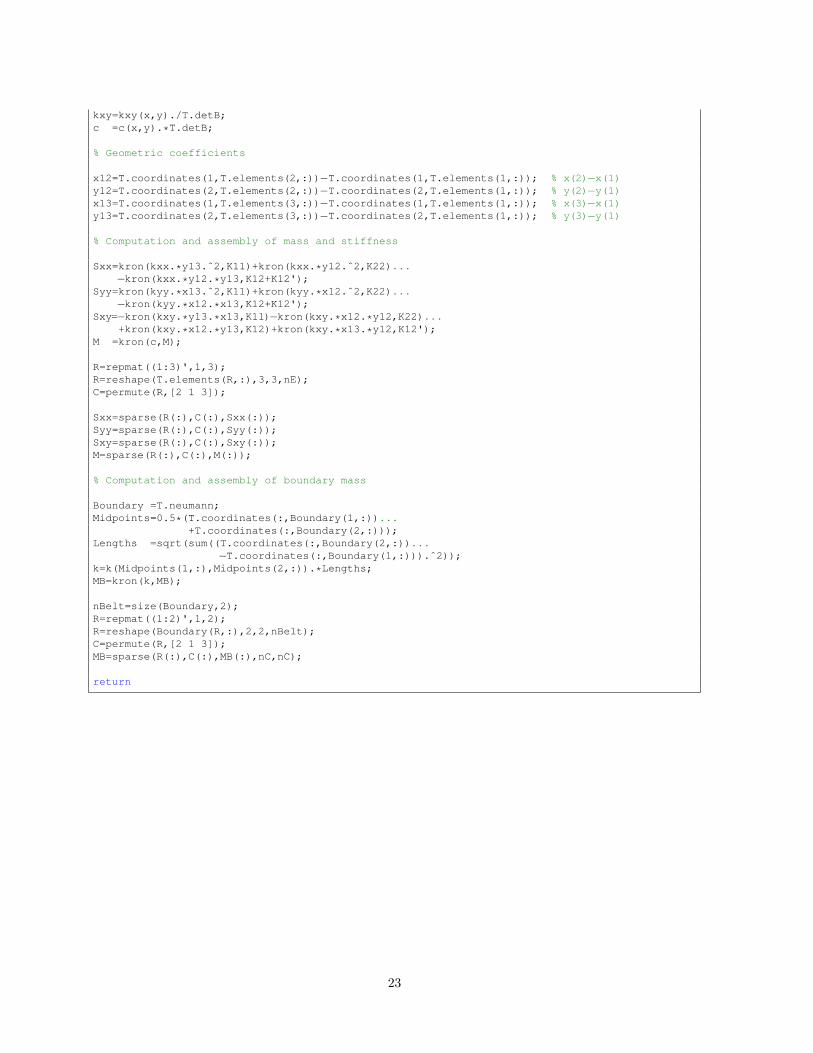
kxy=kxy(x,y)./T.detB;c =c(x,y).*T.detB;

% Geometric coefficients

x12=T.coordinates(1,T.elements(2,:))−T.coordinates(1,T.elements(1,:)); % x(2)−x(1)y12=T.coordinates(2,T.elements(2,:))−T.coordinates(2,T.elements(1,:)); % y(2)−y(1)x13=T.coordinates(1,T.elements(3,:))−T.coordinates(1,T.elements(1,:)); % x(3)−x(1)y13=T.coordinates(2,T.elements(3,:))−T.coordinates(2,T.elements(1,:)); % y(3)−y(1)

% Computation and assembly of mass and stiffness

Sxx=kron(kxx.*y13.ˆ2,K11)+kron(kxx.*y12.ˆ2,K22)...−kron(kxx.*y12.*y13,K12+K12');

Syy=kron(kyy.*x13.ˆ2,K11)+kron(kyy.*x12.ˆ2,K22)...−kron(kyy.*x12.*x13,K12+K12');

Sxy=−kron(kxy.*y13.*x13,K11)−kron(kxy.*x12.*y12,K22)...+kron(kxy.*x12.*y13,K12)+kron(kxy.*x13.*y12,K12');

M =kron(c,M);

R=repmat((1:3)',1,3);R=reshape(T.elements(R,:),3,3,nE);C=permute(R,[2 1 3]);

Sxx=sparse(R(:),C(:),Sxx(:));Syy=sparse(R(:),C(:),Syy(:));Sxy=sparse(R(:),C(:),Sxy(:));M=sparse(R(:),C(:),M(:));

% Computation and assembly of boundary mass

Boundary =T.neumann;Midpoints=0.5*(T.coordinates(:,Boundary(1,:))...

+T.coordinates(:,Boundary(2,:)));Lengths =sqrt(sum((T.coordinates(:,Boundary(2,:))...

−T.coordinates(:,Boundary(1,:))).ˆ2));k=k(Midpoints(1,:),Midpoints(2,:)).*Lengths;MB=kron(k,MB);

nBelt=size(Boundary,2);R=repmat((1:2)',1,2);R=reshape(Boundary(R,:),2,2,nBelt);C=permute(R,[2 1 3]);MB=sparse(R(:),C(:),MB(:),nC,nC);

return

23