A Latent Class Extension of Signal Detection Theory, with

MULTIVARIATE BEHAVIORAL RESEARCH 423

Multivariate Behavioral Research, 37 (4), 423-451Copyright © 2002, Lawrence Erlbaum Associates, Inc.

A Latent Class Extension of Signal Detection Theory,with Applications

Lawrence T. DeCarloDepartment of Human Development

Teachers College, Columbia University

A latent class extension of signal detection theory is presented and applications areillustrated. The approach is useful for situations where observers attempt to detect latentcategorical events or where the goal of the analysis is to select or classify cases. Signaldetection theory is shown to offer a simple summary of the observers’ performance interms of detection and response criteria. Implications of the view via signal detection forthe training of raters are noted, as are approaches to validating the parameters andclassifications. An extension of the signal detection model to more than two latent classes,with a simple restriction on the detection parameters, is introduced. Sample programs tofit the models using software for latent class analysis or software for second generationstructural equation modeling are provided.

In many situations in psychology, education, and medicine, observersattempt to detect or discriminate between two or more classes of events.When the events are observable, the methods of signal detection theory(SDT) can be used to obtain a measure of an observer’s ability to detect ordiscriminate (see Macmillan & Creelman, 1991; Swets, 1996). Consider, forexample, a simple test of recognition memory. A list of words can bepresented during a study period and a combination of old words (from the list)and new words can be presented during a subsequent test, with theobservers’ task being to decide whether each word is old or new, or to ratetheir confidence that a word is old or new. From the perspective of SDT, theeffect of an event (an old or new word) can be represented by a continuouslatent variable, usually interpreted as an observer’s perception of the event(e.g., the familiarity of the word), which is used together with a responsecriterion to arrive at a decision of old or new. The results can be summarizedby a detection parameter, say d, which for the memory example is a measureof recognition memory strength, and by a parameter c that indicates thelocation of the response criterion; the location of the criterion is viewed as

Correspondence concerning this article should be addressed to Lawrence T. DeCarlo,Department of Human Development, Box 118, Teachers College, Columbia University, 525West 120th Street, New York, NY 10027-6696. E-mail: [email protected]

L. DeCarlo

424 MULTIVARIATE BEHAVIORAL RESEARCH

being largely arbitrary, in that it depends on motivational and other (usuallyuncontrolled) factors. Indeed, interest in SDT was stimulated in part byexperiments in psychology that showed that although the response criteria ofobservers attempting to detect a signal varied considerably across differentsessions (and could be experimentally manipulated), their detectionremained approximately constant (e.g., Green & Swets, 1988; Swets,Tanner, & Birdsall, 1961). Since then, SDT has been shown to be quiteuseful for the study of cognitive and perceptual processes in psychology.

For the above example, it is known what type of event was presented oneach trial, that is, whether an old or new word was presented. In othersituations, the task is again one of signal detection, but the events are notobserved. Examples are determining whether or not a person has apsychological or physical condition, such as depression or disease, whetheran essay merits a pass or fail, or whether or not a slide shows a tumor. Inthese cases, the true state of the person or object (hereafter referred tosimply as the case) is not known. As before, SDT assumes that the observerhas a perception of the case that is used together with a criterion to arriveat a decision. Thus, the psychological theory is the same, the only differenceis that the events of interest are not observed.

Signal detection theory can readily be applied to this type of situation byincorporating it into a latent class analysis. Latent class analysis (Clogg,1995; Dayton, 1998; Hagenaars, 1993; McCutcheon, 1987) offers modelsthat include unobserved (latent) classes or categories of persons or objects.Although signal detection models with latent classes have been used inmedical applications (c.f. Henkelman, Kay, & Bronskill, 1990; Quinn, 1989),their general applicability in psychology and education is not well known.The present article motivates the use of latent class SDT models andattempts to bridge some gaps between interrelated research in psychology,education, and medicine.

Signal Detection Theory with Latent Classes

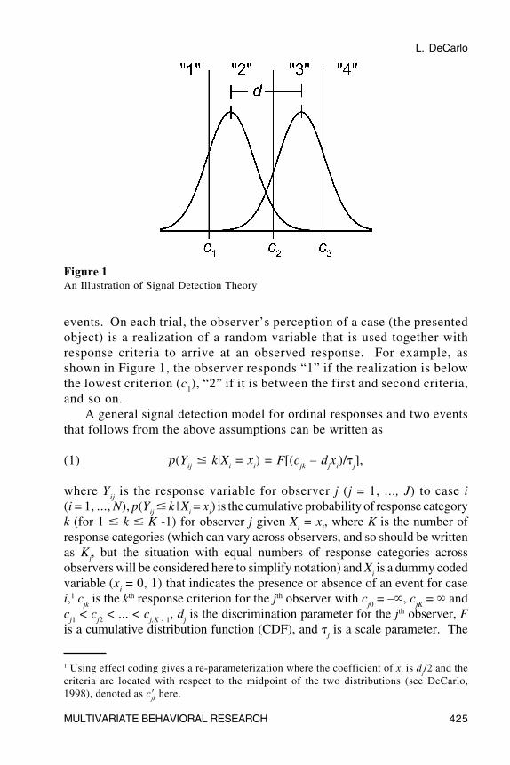
Signal Detection Theory. Figure 1 illustrates the basic ideas ofsignal detection theory for the situation where there are two events (e.g.,signal or noise, old or new word) and the observer uses a one to fourrating response. It is assumed that the presentation of an event to anobserver has an effect that can be represented by a random variable onan underlying continuum (e.g., the observer’s perception). For twoevents, there are two probability distributions that differ in location, asshown in Figure 1. The distance between the distributions, denoted as d,reflects the observer’s ability to discriminate between the two types of

L. DeCarlo


events. On each trial, the observer’s perception of a case (the presentedobject) is a realization of a random variable that is used together withresponse criteria to arrive at an observed response. For example, asshown in Figure 1, the observer responds “1” if the realization is belowthe lowest criterion (c

1), “2” if it is between the first and second criteria,

and so on.A general signal detection model for ordinal responses and two events

that follows from the above assumptions can be written as

(1) p(Yij � k|X

i = x

i) = F[(c

jk – d

jx

i)/�

j],

where Yij is the response variable for observer j (j = 1, ..., J) to case i

(i = 1, ..., N), p(Yij � k | X

i = x

i) is the cumulative probability of response category

k (for 1 � k � K -1) for observer j given Xi = x

i, where K is the number of

response categories (which can vary across observers, and so should be writtenas K

j, but the situation with equal numbers of response categories across

observers will be considered here to simplify notation) and Xi is a dummy coded

variable (xi = 0, 1) that indicates the presence or absence of an event for case

i,1 cjk is the kth response criterion for the jth observer with c

j0 = –�, c

jK = � and

cj1 < c

j2 < ... < c

j,K - 1, d

j is the discrimination parameter for the jth observer, F

is a cumulative distribution function (CDF), and �j is a scale parameter. The

1 Using effect coding gives a re-parameterization where the coefficient of xi is d

j/2 and the

criteria are located with respect to the midpoint of the two distributions (see DeCarlo,1998), denoted as c�

jk here.

Figure 1An Illustration of Signal Detection Theory

L. DeCarlo


logistic CDF is used for the examples presented here, so that the underlyingdistributions are logistic, however the model is more general in that otherdistributions can be used as well; some examples of SDT with normal andextreme value distributions are given in DeCarlo (1998). To use otherdistributions, Equation 1 can be re-written as a generalized linear model, in whichcase the choice of link function determines the form of the underlyingdistributions (see DeCarlo, 1998).

SDT with Latent Events. To extend the model to situations where theevents are latent, the observed variable X is replaced by a latent categoricalvariable, say X* with values x*

c = 0, 1 for c = 1, 2,

(2) p(Yij � k|X* = x*

c) = F[(c

jk – d

jx*

c)/�

j].

The model is the same as before, however the situation differs in thatEquation 2 cannot be fit if there is only one observer (in contrast to Equation 1)because the model is not identified, that is, one cannot obtain uniqueestimates of the parameters. Several observers are necessary for the modelto be identified; for example, for two latent classes, at least three observersare necessary if the responses are dichotomous, whereas at least twoobservers are necessary if the responses are ordinal with at least threecategories. The models for the J observers can then be incorporated into alatent class model, as shown next. Note that the scale parameter �

j can be

set to unity, without loss of generality, and this will be done from here on (thescale parameter has to be taken into account when comparing results frommodels with different link functions; see DeCarlo, 1998).

Latent Class Models. A discussion of latent class analysis is beyond thescope of the present article; the reader is referred to Dayton (1998) or Clogg(1995) for discussion and references. Here it is shown that the signaldetection model given above is easily incorporated into a restricted latentclass model, and some basic aspects of the analysis are illustrated.

Consider the situation where J observers examine N cases and makedecisions in one of K response categories. Note that, for each case, thereis a pattern of responses (a vector) across the observers, which can bedenoted as (Y

1, Y

2, ..., Y

J). The total number of possible response patterns

is KJ; for example, if three observers give ordinal ratings from one to four,then there are 43 = 64 possible response patterns. Thus, the data for Jobservers examining N cases can be summarized by a multiway frequencytable with KJ cells, where each cell gives the number of cases with aparticular response pattern. A latent class model can be viewed as a

L. DeCarlo


probability model for the response patterns. In particular, it is assumed thatthere are C mutually exclusive and exhaustive latent classes so that theprobabilities of the response patterns can be obtained by summing over thelatent classes,

(3) ( ) ( ) ( ) ( )* * *1 2 3 1 2 3 1 2 3

1 1

, , , , , , , | ,C C

c c

p Y Y Y p Y Y Y X p X p Y Y Y X= =

= =∑ ∑

(for J = 3) where p(X* = x*c) is the size (mixing proportion) of latent class c

with p(X*) > 0 for all c and �c p(X* = x*

c) = 1 for c = 1 to C, p(Y

1, Y

2, Y

3) is

the probability of response pattern (Y1, Y

2, Y

3), and p(Y

1, Y

2, Y

3|X*) is the

conditional probability of response pattern (Y1, Y

2, Y

3) given X* = x*

c. In

addition, conditional on the latent class, responses are assumed to beindependent, so that

(4) p(Y1, Y

2, Y

3|X*) = p(Y

1|X*) p(Y

2|X*) p(Y

3|X*),

where p(Yj|X*) is the conditional probability of response k for observer j

given X* and �k p(Y

j = k|X*) = 1. Equation 4 is an assumption of conditional

independence; it reflects a basic assumption of latent class analysis, whichis that the J response variables are independent given the latent class.

Latent Class Models and Signal Detection. Equations 3 and 4 are thebasic equations for an unrestricted latent class model. For restricted latentclass models, the conditional probabilities of Equation 4 are restricted invarious ways. For example, to incorporate the signal detection model ofEquation 2, differences between the cumulative probabilities are used,

(5)

( ) ( )( ) ( ) ( )( ) ( )

* * *

* * * *1

* * *1

| 1

| 1 .

| 1

j c jk j c

j c jk j c jk j c

j c jk j c

p Y k X x F c d x k

p Y k X x F c d x F c d x k K

p Y k X x F c d x k K

−

−

= = = − =

= = = − − − < <

= = = − − =

The result is a general class of signal detection models with latent classes,which are useful for situations that can be conceptualized in terms of SDT,such as when observers attempt to detect or discriminate latent categoricalevents. The models can be fit with software for latent class analysis thatallows one to restrict the conditional probabilities using models with cumulativelink functions. For example, the software LEM (Vermunt, 1997a), which is

L. DeCarlo


freely available on the Internet (http://www.uvt.nl/faculteiten/fsw/organisatie/departementen/mto/software2.html) was used for the analysespresented here; a sample LEM program for the binary response examplediscussed below is given in Appendix A. LEM allows one to fit a variety oflatent class and latent trait models to categorical data using maximumlikelihood; a version of the EM algorithm is used (see Vermunt, 1997a). Fordetails about estimation and the use of the EM algorithm to fit latent classmodels see Bartholomew and Knott (1999), Heinen (1996), McCutcheon,(1987), McLachlan and Peel (2000), or Vermunt (1997b). The modelsconsidered here can also be fit using software for (second generation)structural equation modeling, such as Version 2 of Mplus (Muthén & Muthén,1998); a sample Mplus program for the ordinal response example discussedbelow is given in Appendix A and some other examples are given in DeCarlo(2001).

Examples

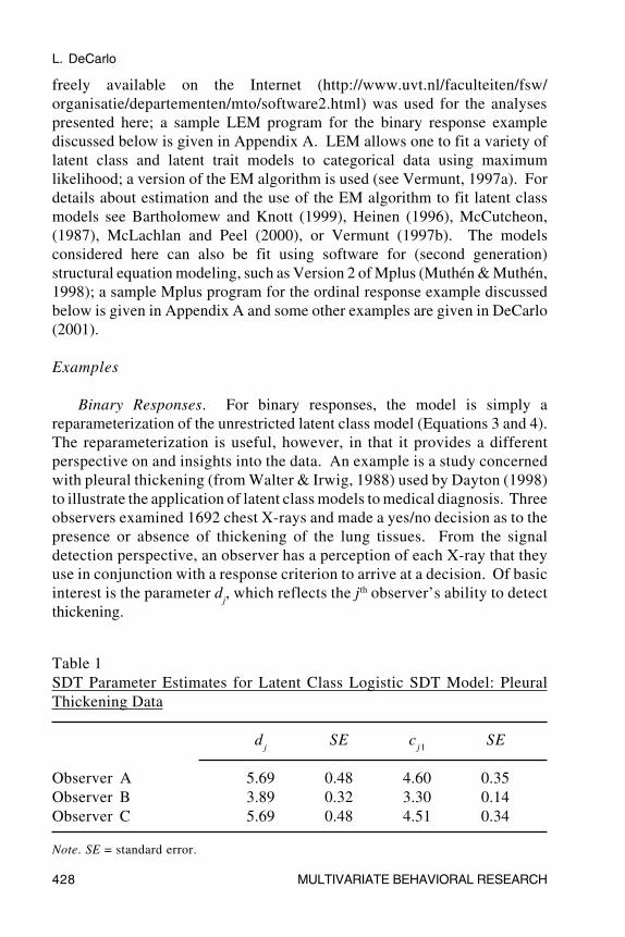
Binary Responses. For binary responses, the model is simply areparameterization of the unrestricted latent class model (Equations 3 and 4).The reparameterization is useful, however, in that it provides a differentperspective on and insights into the data. An example is a study concernedwith pleural thickening (from Walter & Irwig, 1988) used by Dayton (1998)to illustrate the application of latent class models to medical diagnosis. Threeobservers examined 1692 chest X-rays and made a yes/no decision as to thepresence or absence of thickening of the lung tissues. From the signaldetection perspective, an observer has a perception of each X-ray that theyuse in conjunction with a response criterion to arrive at a decision. Of basicinterest is the parameter d

j, which reflects the jth observer’s ability to detect

thickening.

Table 1SDT Parameter Estimates for Latent Class Logistic SDT Model: PleuralThickening Data

dj

SE cj1

SE

Observer A 5.69 0.48 4.60 0.35Observer B 3.89 0.32 3.30 0.14Observer C 5.69 0.48 4.51 0.34

Note. SE = standard error.

L. DeCarlo


Table 1 presents results for a fit of a latent class logistic signal detectionmodel (the data are given by Dayton, 1998, p. 26); a sample LEM programis given in Appendix A and some notes on using LEM are given in AppendixB. First note that the estimates of d

j are all large, significant, and suggest

excellent detection. For the logistic SDT model, dj are simply log odds ratios,

and so the estimate of 3.89 for Observer B (the smallest estimate) indicatesthat his or her odds of detecting thickening are exp(3.89) = 49 times higherfor an event (thickening) than a non-event (no thickening), which is quitegood, as was also noted by Dayton (1998). Note that another (equivalent)view of d

j is that it provides a measure of the conditional precision of each

observer (c.f., Clogg & Manning, 1996; Mellenberg, 1996); for a correlation-type measure, d

j can be rescaled to a zero-one range as follows

Qe

ej

d

d

j

j= −

+1

1,

which is simply Yule’s Q (see Clogg & Manning, 1996). For the pleural thickeningdata, the values of Q

j are .99, .96, and .99 for Observers A, B, and C, respectively,

which again indicates high precision (i.e., good detection) for each observer.The parameter estimates in Table 1 suggest that d

j is equal for Observers

A and C. The first row of Table 2 presents a likelihood ratio (LR) goodnessof fit test for a model with this restriction (note that the unrestricted modelhas as many parameters as observations and so fits perfectly). The LRstatistic is not significant, and so the model is not rejected. In contrast, the

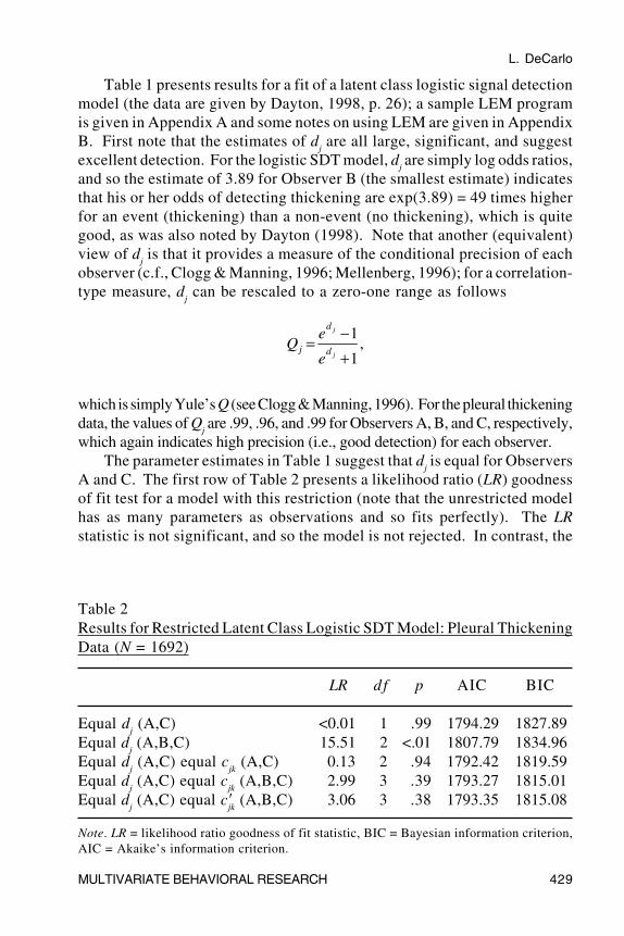
Table 2Results for Restricted Latent Class Logistic SDT Model: Pleural ThickeningData (N = 1692)

LR df p AIC BIC

Equal dj (A,C) <0.01 1 .99 1794.29 1827.89

Equal dj (A,B,C) 15.51 2 <.01 1807.79 1834.96

Equal dj (A,C) equal c

jk (A,C) 0.13 2 .94 1792.42 1819.59

Equal dj (A,C) equal c

jk (A,B,C) 2.99 3 .39 1793.27 1815.01

Equal dj (A,C) equal c�

jk (A,B,C) 3.06 3 .38 1793.35 1815.08

Note. LR = likelihood ratio goodness of fit statistic, BIC = Bayesian information criterion,AIC = Akaike’s information criterion.

L. DeCarlo


second row of Table 2 shows that a model with a restriction of equal dj across

all three observers is rejected. Thus, the results suggest that Observers Aand C detected equally well, whereas detection for Observer B was lower,although his or her detection was still quite good.

Further restrictions that can be considered are with respect to the responsecriteria, although these are usually viewed in SDT as being arbitrary (and so notof substantive interest). Here I simply note that some of the submodelsconsidered by Dayton (1998) have a straightforward interpretation in terms ofSDT. For example, the third row of Table 2 shows that a model with bothdetection and criteria restricted to be equal across Observers A and C is notrejected; this corresponds to submodel III of Dayton (see his Table 3.2, p.28;note that the results obtained with LEM exactly match those shown in Dayton’stable). The fourth row shows that a model with detection equal across A andC and the criterion equal across all three observers is not rejected; thiscorresponds to submodel V of Dayton. Note, however, that there are differentcriterion measures that have been considered in SDT, and tests concerned withthe criterion can give different results, depending on which measure is used. Forexample, the distance of the criterion from the mode of the lower distribution isused here (which distribution is lower can be determined by the output; seeAppendix B), however an alternative measure locates the criterion with respectto its distance from the midpoint of the two (symmetric) distributions (e.g., asdone in the choice theory parameterization of SDT; see DeCarlo, 1998;Macmillan & Creelman, 1991). The last row of Table 2 shows a model with thecriterion equal across the three observers for this alternative measure, denotedas c�

jk (where for symmetric distributions c�

jk = c

jk –½ d

j). In this case, the LR

goodness of fit statistic differs only slightly from before and the model is notrejected (thus one cannot distinguish between alternate hypotheses about thecriterion in this case). Nevertheless, it is important to keep in mind that the resultsof tests concerned with the criterion can differ for the different measures.

Table 2 also shows information criteria, and in particular Akaike’sinformation criterion (AIC) and the Bayesian information criterion (BIC; seeBurnham & Anderson, 1998; Dayton, 1998; Lin & Dayton, 1997), using versionsbased on the log-likelihood. The information criteria can be used to comparenon-nested models, with smaller values indicating a better model; they can beused, for example, to compare models with different link functions, as shownbelow. Table 2 shows that AIC favors the model given in the third row whereasBIC favors the models given in the last two rows (c.f., Dayton, 1998, who alsonoted differences between AIC and BIC for this example). From theperspective of SDT, these models only differ with respect to whether ObserverB had the same criterion location as the other observers, whereas both modelsare consistent with the conclusion that Observers A and C had equal detection.

L. DeCarlo


Finally, the estimates of the latent class size [i.e., p(X*) in Equation 3] are.95 for the lower latent class and .05 for the higher class; note that Dayton(1998) obtained the same values for the (different) models he considered.Thus, it is estimated that about 5% of the 1692 cases had pleural thickening.

In summary, a fit of the latent class signal detection model offers a simpleinterpretation of the data. The analysis suggests that all three observersdetected well, with Observers A and C equal and Observer B lower. Withrespect to the response criterion, it is clarified that there are different types ofrestrictions across observers that can be examined; namely whether thecriterion location is constant with respect to the lower distribution (in which casethe observer is basically controlling the false alarm rate) or whether it is constantwith respect to the midpoint of the two distributions; some implications of thedifferent criterion measures have been considered in SDT (see Macmillan &Creelman, 1991), but merit further study. It is also noted that tests of thecriterion may be of little substantive interest, because of the arbitrary aspect ofthe criterion’s location, but this depends on the particular research application.

Ordinal Responses. Further aspects of the approach via SDT areillustrated by an example with ordinal responses. In this case, examinationof the estimated conditional probabilities, as done in latent class analysis(e.g., by Dayton, 1998, for the binary response example discussed above),may not be as informative as examination of the signal detection parameters.

The example is from a widely cited article by Landis and Koch (1977)where guidelines as to interpreting the magnitude of kappa (Cohen, 1960)were offered (i.e., < 0 = poor, .00-.20 = slight, .21-.40 = fair, .41-.60 = moderate,.61-.80 = substantial, .81-1.00 = almost perfect, p.165; note that Fleiss, 1981,p.218, suggested < .40 as poor agreement, .40 to .75 as fair to good agreement,and > .75 as excellent agreement; in psychometrics, agreement less than .70is generally considered poor). Two neurologists examined patient records andmade a decision as to the presence or absence of multiple sclerosis; the datafor 149 Winnipeg patients are examined here (the data are given in Landis &Koch, 1977); for other analyses of these data, see Darroch and McCloud(1986) and Uebersax (1993b). Decisions with respect to the presence orabsence of multiple sclerosis were made on a 1 to 4 scale, with 1 = certainmultiple sclerosis, 2 = probable multiple sclerosis, 3 = possible multiplesclerosis, and 4 = doubtful, unlikely, or definitely not multiple sclerosis (thecoding is reversed for the analysis presented here, so that higher numbersindicate a diagnosis of more probable multiple sclerosis). SDT assumes thatthe neurologists had a perception of symptoms for each patient, which theyused together with response criteria to arrive at a response.

L. DeCarlo


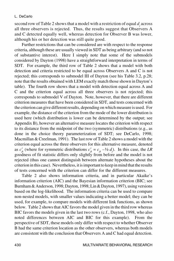
For the sample of 149 patients, kappa is .21, indicating slight agreement,according to the criteria suggested by Landis and Koch (1977) or pooragreement, by Fleiss’ (1981) criteria; weighted kappa (Cohen, 1968) is .38,which also indicates poor agreement. Latent class SDT, on the other hand,offers additional information of interest, such as estimates of the observers’detection and response criteria, the sizes of the latent classes, and theaccuracy of classifications based on the fitted model.

The upper half of Table 3 shows the parameter estimates and standarderrors for a fit of a latent class logistic SDT model. It is apparent that theestimated detection parameters are close in magnitude across the twoobservers. Also note that some of the standard errors are large, which reflectsa lack of precision with respect to estimation, or what Vermunt and Magidson(2000) refer to as “weak identification”; this is also indicated by the ratio of thelargest to smallest eigenvalues of the information matrix (the eigenvalues aregiven in the LEM output), which in this case is 109.58/0.08 = 1370, which israther large. The lack of precision is due to the small sample size relative tothe number of observers. That is, the precision of estimation depends onboth the number of observers and on the sample size: with few observers,larger sample sizes are needed (for example, note that, in contrast to thecurrent example, the ratio of eigenvalues for the binary response examplediscussed above with three observers and 1692 cases is 294.1/2.7 = 109),

Table 3Parameter Estimates for Logistic Latent Class Signal Detection Model:Multiple Sclerosis Data

Unrestricted Model

dj

SE cj1

SE cj2

SE cj3

SE

Neurologist A 4.02 1.79 –0.36 0.38 1.99 1.28 4.21 1.76Neurologist B 4.03 1.84 –0.82 0.35 –0.01 0.39 2.43 1.46

Restricted Model (equal dj)

dj

SE cj1

SE cj2

SE cj3

SE

Neurologist A 4.02 0.45 –0.36 0.34 1.99 0.55 4.22 0.51Neurologist B 4.02 0.45 –0.82 0.34 –0.01 0.35 2.43 0.55


L. DeCarlo


whereas having more observers compensates for a small sample size;2 asimilar point has recently been made in the context of confirmatory factoranalysis by Marsh, Hau, Balla, and Grayson (1998).

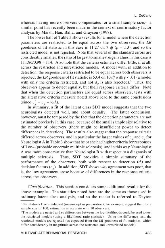
The lower half of Table 3 shows results for a model where the detectionparameters are restricted to be equal across the two observers; the LRgoodness of fit statistic in this case is 11.27 on 7 df (p = .13), and so therestricted model is not rejected. Note that several of the standard errors areconsiderably smaller; the ratio of largest to smallest eigenvalues in this case is111.86/0.98 = 114. Also note that the criteria estimates differ little, if at all,across the restricted and unrestricted models. A model with, in addition todetection, the response criteria restricted to be equal across both observers isrejected; the LR goodness of fit statistic is 53.4 on 10 df with p < .01 (a modelwith only the criteria restricted, and not d

j, is also rejected).3 Thus, the

observers appear to detect equally, but their response criteria differ. Notethat when the detection parameters are equal across observers, tests withthe alternative criteria measure noted above lead to the same conclusions(since c�

jk = c

jk – ½d

j).

In summary, a fit of the latent class SDT model suggests that the twoneurologists detected well, and about equally. The latter conclusion,however, must be tempered by the fact that the detection parameters are notestimated precisely in this case, because of the small sample size relative tothe number of observers (there might be insufficient power to detectdifferences in detection). The results also suggest that the response criteriadiffered across observers, and in particular the larger values of c

j2 and c

j3 for

Neurologist A in Table 3 show that he or she had higher criteria for responsesof 3 or 4 (probable or certain multiple sclerosis), and in this way NeurologistA was more conservative than Neurologist B with respect to a diagnosis ofmultiple sclerosis. Thus, SDT provides a simple summary of theperformance of the observers, both with respect to detection (d

j) and

decision factors (cjk). In addition, SDT shows why agreement was poor, that

is, the low agreement arose because of differences in the response criteriaacross the observers.

Classification. This section considers some additional results for theabove example. The statistics noted here are the same as those used inordinary latent class analysis, and so the reader is referred to Dayton

2 Simulations I’ve conducted (manuscript in preparation), for example, suggest that, for asample size of 100, estimation is accurate with 10 observers.3 The models are nested and so differences between the log-likelihoods could be used to testthe restricted models (using a likelihood ratio statistic). Using the difference test, therestricted models are rejected (as expected from the LR goodness of fit statistics, whichdiffer considerably in magnitude across the restricted and unrestricted models).

L. DeCarlo


(1998) or Clogg (1995) for further discussion and references. The focushere is on the use of the statistics in the context of latent class signaldetection analysis.

A practical goal is to classify the cases into one of the latent classes usingthe observed response patterns. This can be done using the posteriorprobability of X* for a given response pattern, which for three observers canbe written as p(X*|Y

1, Y

2, Y

3). Note that, from Bayes’ theorem,

(6) ( ) ( ) ( )( ) ( )

* *1 2 3*

1 2 3* *

1 2 31

, , || , , ,

, , |C

c

p X p Y Y Y Xp X Y Y Y

p X p Y Y Y X=

=∑

which shows that the posterior probabilities are determined by the latentclass sizes, p(X*) and by p(Y

1, Y

2, Y

3|X*) the latter of which depends on the

signal detection parameters, as shown by Equations 4 and 5. Thus, givenestimates of the latent class sizes, the criteria, and the detection parameters,Equation 6 can be used to assign each case to the latent class for which itsestimated posterior probability of class membership is highest (Goodman, 1974).

It is also of interest to measure the quality of the classifications. First,note that the estimated posterior probabilities can be used to obtain anestimate of the expected proportion of cases correctly classified (see Clogg,1995; Dayton, 1998),

(7) ( )*1 2 3max | , , / ,C s

s

P n p X Y Y Y N = × ∑

(again illustrated for J = 3 observers) where s indicates each unique responsepattern (e.g., there are S = KJ unique patterns, as noted above), n

s is the

frequency of each pattern (i.e., number of cases with a particular pattern;note that either observed or estimated frequencies can be used, as noted byClogg, 1995), max p(X*|Y

1, Y

2, Y

3) is the maximum posterior probability

(across the latent classes) for a given response pattern, and N is the totalnumber of cases. In words, if the maximum estimated posterior probabilityfor a particular response pattern was, for example, .70 for Class 1, then onewould expect that classifying all cases with that response pattern into Class1 would result in 70 percent of the cases being correctly classified. For theentire sample (and all the response patterns), the expected proportioncorrectly classified is then simply a weighted average of the maximumposterior probabilities for each pattern, as shown by Equation 7.

L. DeCarlo


Next, note that if one simply classifies all the cases (i.e., the entiresample) into the latent class with the largest size, then one can expect tocorrectly classify that proportion of cases (i.e., by chance). A statistic thatcorrects for this is lambda, which can be written as

(8)( )

( )*

*

max,

1 max

CP p X

p X

−=

−�

Equation 8 shows that values of lambda greater than zero indicate that usingthe posterior probabilities to classify cases gives an increase in the proportioncorrectly classified over and above that obtained by simply assigning allcases to the latent class with the largest size. Another (equivalent) view oflambda is that it reflects the relative reduction in classification error (Clogg,1995; Goodman & Kruskal, 1954), where the classification error is simplyone minus P

C.

With respect to the multiple sclerosis data, the estimated latent class sizesare .36 and .64 for Classes 1 and 2, respectively, with Class 2 representing thehigher event, which can be interpreted as consisting of patients who possiblyhave multiple sclerosis. The estimate of the proportion correctly classified is.94, and so the estimate of lambda is (.94 – .64)/(1 – .64) = .83, which meansthat there is a relative increase of 83% in the proportion correctly classifiedby using the observers’ response patterns over simply classifying all casesinto the latent class with the largest size. This suggests good classification,although it should be noted that there is an upward bias in the estimate of theproportion correctly classified, because estimation and classification areperformed on the same set of data; to take this into account, Clogg (1995)suggested an approach based on multiple imputation (which merits furtherresearch).

In summary, the example shows that one can have good detection butpoor agreement, in this case because the response criteria differed acrossthe observers, and similarly, one can have good classification but pooragreement (classification depends on detection, the latent class sizes, and thenumber of observers). The latter point is relevant because in practice thegoal is often to classify cases. Thus, it is important to determine if pooragreement arises because detection is poor, in which case classificationmight also be poor (this depends in part on how many observers there are),or if agreement is poor because of differences in the criteria acrossobservers, as in the current example, in which case classification might begood (e.g., if detection is good). The relevant information is provided by theestimates of the detection and criteria parameters from the SDT analysis.

L. DeCarlo


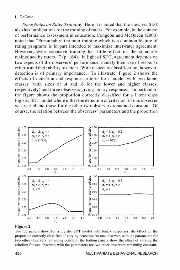
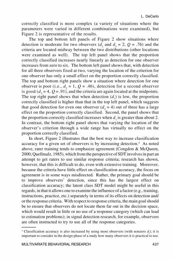
Some Notes on Rater Training. Here it is noted that the view via SDTalso has implications for the training of raters. For example, in the contextof performance assessment in education, Congdon and McQueen (2000)noted that “Presumably, the rater training which is a common feature ofrating programs is in part intended to maximize inter-rater agreement.However, even extensive training has little effect on the standardsmaintained by raters...” (p. 164). In light of SDT, agreement depends ontwo aspects of the observers’ performance, namely their use of responsecriteria and their ability to detect. With respect to classification, however,detection is of primary importance. To illustrate, Figure 2 shows theeffects of detection and response criteria for a model with two latentclasses (with sizes of .4 and .6 for the lower and higher classes,respectively) and three observers giving binary responses. In particular,the figure shows the proportion correctly classified for a latent classlogistic SDT model where either the detection or criterion for one observerwas varied and those for the other two observers remained constant. Ofcourse, the relation between the observers’ parameters and the proportion

Figure 2The top panels show, for a logistic SDT model with binary responses, the effect on theproportion correctly classified of varying detection for one observer, with the parameters fortwo other observers remaining constant; the bottom panels show the effect of varying thecriterion for one observer, with the parameters for two other observers remaining constant.

L. DeCarlo


correctly classified is more complex (a variety of situations where theparameters were varied in different combinations were examined), butFigure 2 is representative of the results.

The top and bottom left panels of Figure 2 show situations wheredetection is moderate for two observers (d

2 and d

3 = 2, Q = .76) and the

criteria are located midway between the two distributions (other locationswere examined as well). The top left panel shows that the proportioncorrectly classified increases nearly linearly as detection for one observerincreases from zero to six. The bottom left panel shows that, with detectionfor all three observers fixed at two, varying the location of the criterion forone observer has only a small effect on the proportion correctly classified.The top and bottom right panels show a situation where detection for oneobserver is poor (i.e., d

2 = 1, Q = .46), detection for a second observer

is good (d3 = 4, Q = .91), and the criteria are again located at the midpoints.

The top right panel shows that when detection (d1) is low, the proportion

correctly classified is higher than that in the top left panel, which suggeststhat good detection for even one observer (d

3 = 4) out of three has a large

effect on the proportion correctly classified. Second, the panel shows thatthe proportion correctly classified increases when d

1 is greater than about 2.

In contrast, the bottom right panel shows that varying the location of theobserver’s criterion through a wide range has virtually no effect on theproportion correctly classified.

In short, Figure 2 illustrates that the best way to increase classificationaccuracy for a given set of observers is by increasing detection.4 As notedabove, rater training tends to emphasize agreement (Congdon & McQueen,2000; Quellmalz, 1985), which from the perspective of SDT involves in part anattempt to get raters to use similar response criteria; research has shown,however, that this is difficult to do, even with extensive training. Moreover,because the criteria have little effect on classification accuracy, the focus onagreement is in some ways misdirected. Rather, the primary goal should beto improve observers’ detection, since this has the largest effect onclassification accuracy; the latent class SDT model might be useful in thisregards, in that it allows one to examine the influence of a factor (e.g., training,instructions, practice, etc.) separately in terms of its effects on detection and/or the response criteria. With respect to response criteria, the main goal shouldbe to ensure that observers do not locate them far out in the decision space,which would result in little or no use of a response category (which can leadto estimation problems); in signal detection research, for example, observersare often instructed to try to use all of the response categories.

4 Classification accuracy is also increased by using more observers (with nonzero dj); it is

important to consider in the design phase of a study how many observers it is practical to use.

L. DeCarlo


Validation

As with any model, issues arise as to the validity of the model, itsinterpretation, and its application within a particular substantive context.Two basic aspects that should be assessed are the validity of theclassifications and the validity of the SDT parameters.

Assessing Classification. This aspect of validation is the same as forordinary latent class analysis, and so will only be briefly touched upon;examples of validation in latent class analysis can be found in Aitkin,Anderson, and Hinde (1981), Dayton (1998), and in chapters in Rost andLangeheine (1997). In some situations, information about the true states ofcases might be available or might become available at a later time (e.g., inmedicine or psychology); the known cases can then be used to validate theclassifications. In other situations, known cases might not be available, butsome other type of information might be available that can be used to validatethe classifications (e.g., criterion validity). For example, in educationalapplications such as writing assessment, grades on exams or grade pointaverage are often used as criteria in this way.

An issue that arises when known cases are not available is whether thelatent classes correspond exactly to true categories. Uebersax (1988) noted,for example, that assuming an identity between the latent classes and truecategories “is not implausible in many cases” (p. 409), but this has been atopic of some debate; for a discussion of this and other issues in the contextof latent class analysis and item response theory, see Uebersax (1988) andthe references therein. Here it is noted that, for a particular application, theidentity issue should be considered, and, as part of the study design, oneshould consider what type of evidence as to validity can be obtained (e.g.,criterion variables).

Assessing SDT Parameters. With respect to assessing the signaldetection parameters, a basic question of interest is whether or not theestimated d

j actually reflect the observers’ ability to discriminate between

latent events. This can be assessed in several ways, depending on whether ornot cases with known statuses are available. If they are, then one approachwould be to use the known cases in another session with the same set ofobservers. The estimates of d

j could then be compared to those obtained in

a session using unknown cases (note that the data from both sessions could befit simultaneously); if the values were similar across the sessions (or perhapsjust had a similar rank ordering), then that would suggest that the d

j reflect

some basic aspect of the observers, such as their ability to discriminate.

L. DeCarlo


The availability of known cases also offers other interesting possibilities.For example, estimation might be improved if one can include a proportionof known cases in with the unknown cases in the rating session; this isdiscussed as partial classification in mixture analysis (McLachlan & Peel,2000) or as training data in the Mplus user’s guide (Muthén & Muthén, 1998);note that a latent class signal detection model with partial classification canbe fit using Mplus or LEM.

The situation is more complex in the absence of known cases. First, itis useful to note that a similar problem exists in item response theory and inconfirmatory factor analysis; validating d, for example, is analogous tovalidating the discrimination parameter in item response theory or the factorloadings in confirmatory factor analysis. An approach similar to that usedin those areas can be applied. For example, it would be of basic interest todetermine if detection was invariant for a given set of observers overrepeated sessions; similar values of d

j across sessions would provide

evidence that dj measures a stable characteristic. This is analogous to

research in item response theory that has studied the invariance of itemparameters across different groups of examinees (see Hambleton &Swaminathan, 1985; Lord, 1980) or over time (e.g., Hoskens & Wilson,2001), and to research in confirmatory factor analysis that has studied theinvariance of factor loadings across groups or time (e.g., Alwin & Jackson,1981; Byrne, Shavelson, & Muthén, 1989). Note that, from the view viaSDT, one would expect that discrimination might be invariant, but not thecriteria (so there is only a partial invariance); also note that conclusions withrespect to the criteria can differ, depending on which criteria measure isused, as discussed previously.

A useful aspect of the view via SDT is that it also suggests newexperiments. For example, it would be interesting to try to induce observersto vary their criteria across different sessions, say by varying theinstructions, and to see the effect, if any, on the SDT parameters, which isanalogous to earlier research in experimental psychology with known cases;this could provide evidence for the validity of the criteria (e.g., if they can besystematically affected by instructions) and/or the detection parameter(e.g., if it is stable as the criteria vary). One could also try to experimentallymanipulate discrimination, perhaps by varying factors such as amount ofpractice. Another possibility would be to use a contrasted-groups approach.For example, instead of using expert raters as gold standards (i.e., errorfree), one can allow for error in their judgments and compare them to a groupof non-experts; the model could be fit to the data of both groupssimultaneously and the estimated discrimination parameters compared;higher values for the experts could be viewed as evidence that d

j reflects an

L. DeCarlo


observer’s ability to discriminate. These and other possibilities remain to beexplored in future research.

Extensions

The focus here has been on the utility of the two class signal detectionmodel, but there are several ways the basic model can be extended. Thesecan be classified as extensions with respect to the signal detection part of themodel or with respect to the latent classes, such as increasing their numberor including additional latent variables.

With regards to extensions of the signal detection model, note thatalthough the focus here has been on the logistic model with ordinal responses,the model is actually more general in that different link functions can be used,and so a wide range of models can be considered. Examples of usingdifferent link functions with SDT models for observed events are given inDeCarlo (1998); an example with latent events is given below. Otherpossibilities are to allow the variances of the underlying distributions to differacross the latent classes, as in the unequal variance extension of the signaldetection model for observed events (Green & Swets, 1988), or to use amixture extension of SDT (DeCarlo, 2002).

Other extensions are with respect to the latent classes. One option is toincrease the number of latent classes. As discussed next, an interestingextension is to increase the number of latent classes, but with a restrictionon the discrimination parameters.

An Equal Distance SDT Model. In the two class SDT model, the valuesfor x*

c = 0, 1 for c = 1, 2 and p(X*) is estimated. One extension uses more

values for X* and in particular x*c = 0, 1, ..., C – 1 for the c = 1 to C latent

classes. Here I note that SDT provides a simple interpretation of theresulting model. The approach is similar to that used in log-linear associationmodels, as discussed by Clogg (1988), with the difference that the later areformulated within a log-linear framework (i.e., the models use adjacentcategory logits, not cumulative links). The extended SDT model discussedhere (with logit link) can be viewed as a latent class extension of the uniformassociation model for cumulative odds ratios discussed by Agresti (1990); itis also more general in that other links can be used.

Specifically, let the values of X* be x*c = 0, 1, ..., C – 1 with p(X*) free,

as in the basic two class model (still with a sum to one constraint on theprobabilities). This is tantamount to assuming that the C underlyingdistributions are ordered and equally spaced within each observer. That is,Equation 2 shows that with this coding scheme, d

j2 = 2d

j1, where d

j1 is the

L. DeCarlo


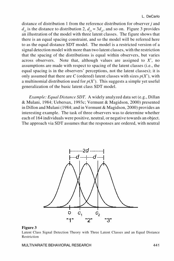
distance of distribution 1 from the reference distribution for observer j andd

j2 is the distance to distribution 2, d

j3 = 3d

j1, and so on. Figure 3 provides

an illustration of the model with three latent classes. The figure shows thatthere is an equal spacing constraint, and so the model will be referred hereto as the equal distance SDT model. The model is a restricted version of asignal detection model with more than two latent classes, with the restrictionthat the spacing of the distributions is equal within observers, but variesacross observers. Note that, although values are assigned to X*, noassumptions are made with respect to spacing of the latent classes (i.e., theequal spacing is in the observers’ perceptions, not the latent classes); it isonly assumed that there are C (ordered) latent classes with sizes p(X*), witha multinomial distribution used for p(X*). This suggests a simple yet usefulgeneralization of the basic latent class SDT model.

Example: Equal Distance SDT. A widely analyzed data set (e.g., Dillan& Mulani, 1984; Uebersax, 1993c; Vermunt & Magidson, 2000) presentedin Dillon and Mulani (1984; and in Vermunt & Magidson, 2000) provides aninteresting example. The task of three observers was to determine whethereach of 164 individuals were positive, neutral, or negative towards an object.The approach via SDT assumes that the responses are ordered, with neutral

Figure 3Latent Class Signal Detection Theory with Three Latent Classes and an Equal DistanceRestriction

L. DeCarlo


between positive and negative (responses were coded as 1 = negative, 2 =neutral, and 3 = positive). Dillon and Mulani (1984) noted that an unrestrictedlatent class model with three classes provided a good fit of the data (severalof the smallest eigenvalues are zero, however, which indicates an empiricalidentification problem; Dillon and Mulani noted that they added a constant tothe table cells, which is not done here).

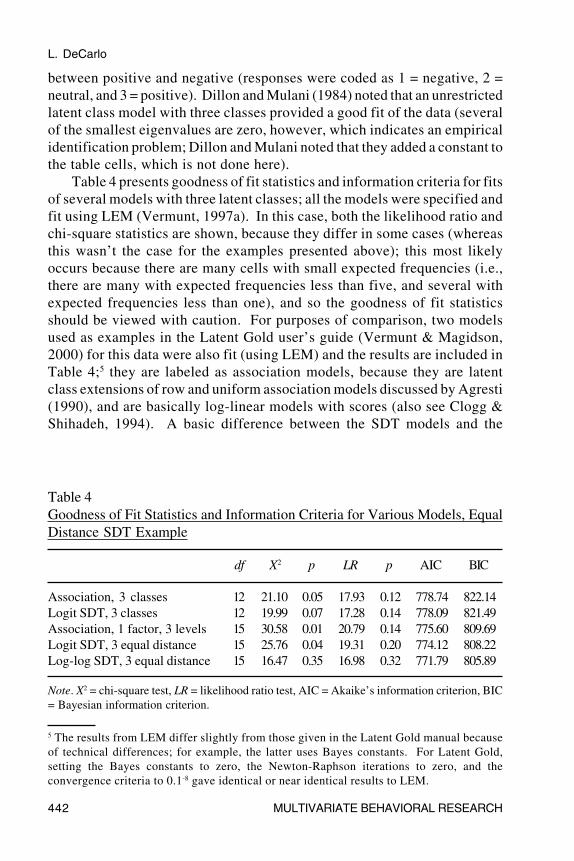
Table 4 presents goodness of fit statistics and information criteria for fitsof several models with three latent classes; all the models were specified andfit using LEM (Vermunt, 1997a). In this case, both the likelihood ratio andchi-square statistics are shown, because they differ in some cases (whereasthis wasn’t the case for the examples presented above); this most likelyoccurs because there are many cells with small expected frequencies (i.e.,there are many with expected frequencies less than five, and several withexpected frequencies less than one), and so the goodness of fit statisticsshould be viewed with caution. For purposes of comparison, two modelsused as examples in the Latent Gold user’s guide (Vermunt & Magidson,2000) for this data were also fit (using LEM) and the results are included inTable 4;5 they are labeled as association models, because they are latentclass extensions of row and uniform association models discussed by Agresti(1990), and are basically log-linear models with scores (also see Clogg &Shihadeh, 1994). A basic difference between the SDT models and the

5 The results from LEM differ slightly from those given in the Latent Gold manual becauseof technical differences; for example, the latter uses Bayes constants. For Latent Gold,setting the Bayes constants to zero, the Newton-Raphson iterations to zero, and theconvergence criteria to 0.1-8 gave identical or near identical results to LEM.

Table 4Goodness of Fit Statistics and Information Criteria for Various Models, EqualDistance SDT Example

df X2 p LR p AIC BIC

Association, 3 classes 12 21.10 0.05 17.93 0.12 778.74 822.14Logit SDT, 3 classes 12 19.99 0.07 17.28 0.14 778.09 821.49Association, 1 factor, 3 levels 15 30.58 0.01 20.79 0.14 775.60 809.69Logit SDT, 3 equal distance 15 25.76 0.04 19.31 0.20 774.12 808.22Log-log SDT, 3 equal distance 15 16.47 0.35 16.98 0.32 771.79 805.89

Note. X2 = chi-square test, LR = likelihood ratio test, AIC = Akaike’s information criterion, BIC= Bayesian information criterion.

L. DeCarlo


association models is that the SDT models use cumulative links whereas theassociation models use adjacent category logits.

The first two models in Table 4 with 12 degrees of freedom are notnested and differ only with respect to the link function. The first is anassociation model that is equivalent to the ordinal indicator, three nominalcluster model discussed by Vermunt and Magidson (2000, see p.138),followed by a latent class logistic SDT model with three latent classes. Thegoodness of fit statistics suggest that the fit of both models is satisfactory.The next three models have 15 df; the first is an association model with onethree level factor, which is referred to by Vermunt and Magidson (2000) asan ordinal three-level factor model with ordinal indicators. Next are twoequal distance three class SDT models with logit and log-log links. Vermuntand Magidson (2000) noted that, of the models they considered, the BICindicated that the association model with one three-level factor was thepreferred model. Table 4 shows that both the AIC and BIC are smaller forthe equal distance SDT models and are smallest for the model with log-loglink (the log-log link implies that the underlying distributions are skewed tothe right). Thus, the results suggest that the three class equal distance SDTmodels provide a parsimonious description of the data.

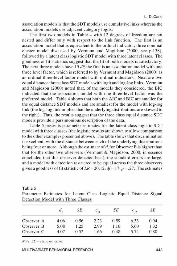
Table 5 presents parameter estimates for the latent class logistic SDTmodel with three classes (the logistic results are shown to allow comparisonto the other examples presented above). The table shows that discriminationis excellent, with the distance between each of the underlying distributionsbeing four or more. Although the estimate of d

j for Observer B is higher than

that for the other two observers (Vermunt & Magidson, 2000, in essenceconcluded that this observer detected best), the standard errors are large,and a model with detection restricted to be equal across the three observersgives a goodness of fit statistic of LR = 20.12, df = 17, p = .27. The estimates

Table 5Parameter Estimates for Latent Class Logistic Equal Distance SignalDetection Model with Three Classes

dj

SE cj1

SE cj2

SE

Observer A 4.06 0.56 2.23 0.59 6.33 0.94Observer B 5.08 1.25 2.99 1.16 5.60 1.32Observer C 4.07 0.52 1.66 0.48 5.74 0.80


L. DeCarlo


of the latent class sizes for the negative, neutral, and positive classes are .21,.36, and .43, respectively, whereas the estimate of P

C = .95 and � = .90 (note

that the latter estimate differs slightly from .91, computed with the valuesreported here, because of rounding).

In summary, the results are concisely and meaningfully summarized interms of the latent class equal distance SDT model: (a) detection is good, (b)the observers do not differ with respect to detection (or there is insufficientinformation to detect differences across observers), (c) the observersperceive the neutral class as being midway between the negative and positiveclasses, and (d) classification appears to be good. Note that a comparison oflatent class models with cumulative link functions to association models meritsfurther attention; the information criteria in Table 4, for example, suggest thatin this case the (SDT) models with cumulative links are preferred over the(association) models with adjacent category logits, but the differences appearto be small (in this example, the models are near equivalent in terms of fit, butnevertheless are conceptually quite different).

Covariates. Another extension of the latent class SDT model is toinclude covariates, as has been done for latent class models (e.g., Dayton &Macready, 1988; van der Heijden, Dessens, & Bockenholt, 1996). The mostgeneral model allows for an effect of covariates on the latent classprobabilities and also direct effects of covariates on the responseprobabilities. Although either or both of these types of effects can beincluded, attention must be given to the interpretation of the resulting model.For example, from the perspective of SDT, allowing the covariates to affectthe response probabilities corresponds to a situation where the covariatesare viewed as factors that affect the observers’ perceptions (usingcovariates in this way is analogous to allowing for a type of differential itemfunctioning in item response theory), whereas allowing them to affect thelatent class probabilities corresponds to a situation where interest centers onusing the covariates to predict latent class membership (e.g., to study groupdifferences, such as across gender or ethnicity; this is analogous to multipleindicator, multiple cause models in structural equation modeling). Researchon the use of covariates in latent class signal detection models is needed.

There are many other applications and extensions that can be considered.For example, the latent class SDT model presented here can also be used insituations where the observers rate only a portion of the cases, as done indesigns with a large number of cases. There are then missing values (bydesign) for each observer (i.e., the cases the observer did not rate). The valuesare missing completely at random (see Little & Rubin, 1987) and the latentclass SDT model can be fit (using LEM, for example) by analyzing subtables

L. DeCarlo


(with appropriate parameter restrictions across tables) and including anindicator variable for the missing values, as discussed by Vermunt (1997a;1997b). Another extension is to relax the assumption of conditionalindependence by, for example, introducing random effects (e.g., Qu, Tan, &Kutner, 1996; Uebersax, 1999). One can also consider multidimensionalmodels with additional categorical or continuous latent variables. Theseremain to be explored in future research. Some issues and limitations shouldalso be noted: larger sample sizes or more observers might be needed foradequate estimation with more complex models, for example, issues ofequivalent or near equivalent models (that possibly lead to differentconclusions) arise, and the need for validation is as important as ever.

Comments on Some Related Models. The latent class SDT model isclosely related to located latent class models (Uebersax, 1993b, 1993c) andto a latent trait finite mixture model discussed by Uebersax (1993a). UsingUebersax’s (1993c) notation (and the subscripts used here), a located latentclass model for ordinal responses can be written as

(9) ( ) ( )1

| , , .1 exp 1.7

ij j j c

j jk c

p Y k BB

� �

� �

≤ = + − −

For two classes, c = 1, 2, the above is equivalent to the two class SDT modelwith a logit link and the following relations between the SDT parameters andthe located latent class parameters: c

jk = �

jk, d

j = 1, �

j = 1/(1.7�

j), B

1 = 0, and

B2 = 1. Uebersax (1993c) refers to �

j as a measurement error parameter;

the above shows that it is equivalent to the inverse of the scale parameter �j

in the SDT model. Note that, because dj is restricted to be unity in the located

latent class model, �j plays the same role as the detection parameter in the

latent class signal detection model; this simply reflects the arbitrary scale: inSDT, d

j is the distance between the underlying distributions with the variance

fixed, whereas in located latent class analysis, the distance B2 – B

1 is fixed

and �j reflects the conditional precision (i.e., the variance of the underlying

distributions). There are also differences in the approaches when applied tomore than two latent classes, a discussion of which is outside the scope ofthe present article.

Another extension is to use a probability distribution for the latentclasses, in which case the models are closely related to discretized versionsof item response models (see Heinen, 1996). For example, using adiscretized normal distribution for p(X*) and a logistic cumulative linkfunction gives a model that is closely related to the graded response model

L. DeCarlo


(Samejima, 1969). The conceptualization of the model differs, however, inthat in SDT randomness arises from an observer’s perception of a casewhereas this is not the view with respect to item response theory. It wouldbe informative to compare the different approaches in future research.

Conclusion

Signal detection theory with latent classes offers a simple andpsychologically motivated approach to situations where observers makejudgments about latent events. The view via SDT suggests that a large bodyof research and theory in psychology is relevant to models used in education,medicine, biostatistics, and psychometrics. There are many directions forfuture research, including experimental studies and comparisons andcontrasts of different models.

References

Agresti, A. (1990). Categorical data analysis. New York: Wiley.Aitkin, M., Anderson, D., & Hinde, J. (1981). Statistical modelling of data on teaching

styles. Journal of the Royal Statistical Society, A, 144, 419-448.Alwin, D. F. & Jackson, D. J. (1981). Applications of simultaneous factor analysis to

issues of factorial invariance. In D. J. Jackson & E. F. Borgatta (Eds.), Factor analysisand measurement in sociological research (pp. 249-279). Beverly Hills, CA: Sage.

Bartholomew, D. J. & Knott, M. (1999). Latent variable models and factor analysis (2nd

ed.). New York: Oxford University Press.Burnham, K. P. & Anderson, D. R. (1998). Model selection and inference: A practical

information-theoretic approach. New York: Springer.Byrne, B. M., Shavelson, R. J., & Muthén, B. (1989). Testing for the equivalence of factor

covariance and mean structures: The issue of partial measurement invariance.Psychological Bulletin, 105, 456-466.

Clogg, C. C. (1988). Latent class models for measuring. In R. Langeheine & J. Rost (Eds.),Latent trait and latent class models (pp. 173-205). New York: Plenum Press.

Clogg, C. C. (1995). Latent class models. In G. Arminger, C. C. Clogg, & M. E. Sobel(Eds.), Handbook of statistical modeling for the social and behavioral sciences (pp.311-359). New York: Plenum Press.

Clogg, C. C. & Manning, W. D. (1996). Assessing reliability of categorical measurementsusing latent class models. In A. von Eye & C. C. Clogg (Eds.), Categorical variablesin developmental research: Methods of analysis (pp. 169-182). New York: AcademicPress.

Clogg, C. C. & Shihadeh, E. S. (1994). Statistical models for ordinal variables. ThousandOaks, CA: Sage.

Cohen, J. (1960). A coefficient of agreement for nominal scales. Educational andPsychological Measurement, 20, 37-46.

Cohen, J. (1968). Weighted kappa: Nominal scale agreement with provision for scaleddisagreement or partial credit. Psychological Bulletin, 70, 213-220.

L. DeCarlo


Congdon, P. J. & McQueen, J. (2000). The stability of rater severity in large-scaleassessment programs. Journal of Educational Measurement, 37, 163-178.

Darroch, J. N. & McCloud, P. I. (1986). Category distinguishability and observeragreement. Australian Journal of Statistics, 28, 371-388.

Dayton, C. M. (1998). Latent class scaling analysis. Thousand Oaks, CA: Sage.Dayton, C. M. & Macready, G. B. (1988). Concomitant-variable latent-class models.

Journal of the American Statistical Association, 83, 173-178.DeCarlo, L. T. (1998). Signal detection theory and generalized linear models.

Psychological Methods, 3, 186-205.DeCarlo, L. T. (2001, July). Signal detection models as structural equation models and

latent class models: Examples of mixture, latent class, and multivariate signaldetection models. Paper presented at the 2001 meeting of the Society forMathematical Psychology, Providence, RI. Available at http://www.columbia.edu/~ld208.

DeCarlo, L. T. (2002). Signal detection theory with finite mixture distributions:Theoretical developments with applications to recognition memory. PsychologicalReview, 109, 710-721.

Dillon, W. R. & Mulani, N. (1984). A probabilistic latent class model for assessing inter-judge reliability. Multivariate Behavioral Research, 19, 438-458.

Fleiss, J. L. (1981). Statistical methods for rates and proportions (2nd ed.). New York:John Wiley & Sons.

Goodman, L. A. (1974). The analysis of systems of qualitative variables when some of thevariables are unobservable. Part I – a modified latent structure approach. AmericanJournal of Sociology, 79, 1179-1259.

Goodman, L. A. & Kruskal, W. H. (1954). Measures of association for crossclassifications. Journal of the American Statistical Association, 49, 732-764.

Green, D. M. & Swets, J. A. (1988). Signal detection theory and psychophysics (Rev. Ed.).Los Altos, CA: Peninsula Publishing.

Hagenaars, J. A. (1993). Loglinear models with latent variables. Newbury Park, CA: Sage.Hambleton, R. K. & Swaminathan, H. (1985). Item response theory. Boston, MA:

Kluwer-Nijhoff Publishing.Heinen, T. (1996). Latent class and discrete latent trait models: Similarities and

differences. Thousand Oaks, CA: Sage.Henkelman, R. M., Kay, I., & Bronskill, M. J. (1990). Receiver operating characteristic

(ROC) analysis without truth. Medical Decision Making, 10, 24-29.Hoskens, M. & Wilson, M. (2001). Real-time feedback on rater drift in constructed-

response items: An example from the Golden State examination. Journal ofEducational Measurement, 38, 121-145.

Landis, J. R. & Koch, G. G. (1977). The measurement of observer agreement for categoricaldata. Biometrics, 33, 159-174.

Lin, T. H. & Dayton, C. M. (1997). Model selection information criteria for non-nestedlatent class models. Journal of Educational and Behavioral Statistics, 22, 249-264.

Little, R. J. A. & Rubin, D. B. (1987). Statistical analysis with missing data. New York:John Wiley & Sons.

Lord, F. M. (1980). Applications of item response theory to practical testing problems.Hillsdale, NJ: Lawrence Erlbaum Associates.

Macmillan, N. A. & Creelman, C. D. (1991). Detection theory: A user’s guide. New York:Cambridge University Press.

L. DeCarlo


Marsh, H. W., Hau, K., Balla, J. R., & Grayson, D. (1998). Is more ever too much? Thenumber of indicators per factor in confirmatory factor analysis. MultivariateBehavioral Research, 33, 181-200.

McCutcheon, A. L. (1987). Latent class analysis. Newbury Park, CA: Sage.McLachlan, G. & Peel, D. (2000). Finite mixture models. New York: John Wiley & Sons.Mellenberg, G. J. (1996). Measurement precision in test score and item response models.

Psychological Methods, 1, 293-299.Muthén, L. K. & Muthén, B. O. (1998). Mplus user’s guide. Los Angeles: Authors.Qu, Y., Tan, M., & Kutner, M. H. (1996). Random effects models in latent class analysis

for evaluating accuracy of diagnostic tests. Biometrics, 52, 797-810.Quellmalz, E. S. (1985). Essay examinations. In T. Husen & T. N. Postlethwaite (Eds.),

International encyclopedia of education: Research and studies (pp.1709-1714). NewYork: Pergamon Press.

Quinn, M. F. (1989). Relation of observer agreement to accuracy according to a two-receiver signal detection model of diagnosis. Medical Decision Making, 9, 196-206.

Rost, J. & Langeheine, R. (Eds.). (1997). Applications of latent trait and latent class modelsin the social sciences. New York: Waxmann Münster.

Samejima, F. (1969). Estimation of latent ability using a response pattern of graded scores.Psychometrika Monograph No. 17, 34.

Swets, J. A. (1996). Signal detection theory and ROC analysis in psychology anddiagnostics: Collected papers. Hillsdale, NJ: Erlbaum.

Swets, J. A., Tanner, W. P., & Birdsall, T. G. (1961). Decision processes in perception.Psychological Review, 68, 301-340.

Uebersax, J. S. (1988). Validity inferences from interobserver agreement. PsychologicalBulletin, 104, 405-416.

Uebersax, J. S. (1993a). A latent trait finite mixture model for the analysis of ratingagreement. Biometrics, 49, 823-835.

Uebersax, J. S. (1993b). LLCA: Located latent class analysis user’s manual. Unpublishedmanuscript, Wake Forest University, Winston-Salem, North Carolina. Available athttp://ourworld.compuserve.com/homepages/jsuebersax/papers.htm.

Uebersax, J. S. (1993c). Statistical modeling of expert ratings on medical treatmentappropriateness. Journal of the American Statistical Association, 88, 421-427.

Uebersax, J. S. (1999). Probit latent class analysis with dichotomous or ordered categorymeasures: Conditional independence/dependence models. Applied PsychologicalMeasurement, 23, 283-297.

Van der Heijden, P. G. M., Dessens, J., & Bockenholt, U. (1996). Estimating theconcomitant-variable latent-class model with the EM algorithm. Journal ofEducational and Behavioral Statistics, 21, 215-229.

Vermunt, J. K. (1997a). LEM: A general program for the analysis of categorical data.Tilburg University, Netherlands: Author. Available at http://www.uvt.nl/faculteiten/fsw/organisatie/departementen/mto/software2.html.

Vermunt, J. K. (1997b). Log-linear models for event histories. Thousand Oaks, CA: SagePublications Inc.

Vermunt, J. K. & Magidson, J. (2000). Latent gold user’s guide. Belmont, MA: StatisticalInnovations.

Walter, S. D. & Irwig, L. M. (1988). Estimates of test error rates, disease prevalence andrelative risk from misclassified data: A review. Journal of Clinical Epidemiology, 41,923-937.

Accepted November, 2001.

L. DeCarlo


Appendix ASample LEM and Mplus Programs

LEM Program

* Binary response example (see Dayton, 1998)* Table 3.1, Pleural thickening data (* denotes

comments)

lat 1 * there is 1 latentvariable (X)

man 3 * there are three manifestvariables (A,B,C)

dim 2 2 2 2 * dimensions of thevariables

lab X A B C * labels for thevariables

mod X * model statement forp(X)

A|X cum(a) {cov(X,1)} * model statements forc o n d i t i o n a lprobabilities

B|X cum(a) {cov(X,1)} * cum(a) gives a logitlink, design for covbelow

C|X cum(a) {cov(X,1)}rec 8 * there are 8 records

in an external filerco * the data include

record countswse separam.txt * write out the

standard errors to“separam.txt”

des [0 1 0 1 0 1] * the design matrix,three dummy coded Xs

dat dayton98.txt * the name of the datafile

L. DeCarlo


Mplus Program

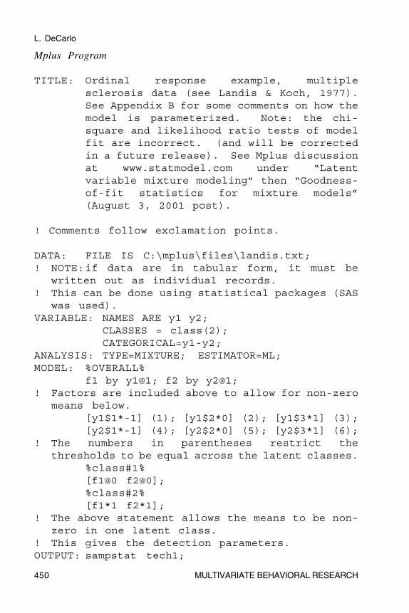
TITLE: Ordinal response example, multiplesclerosis data (see Landis & Koch, 1977).See Appendix B for some comments on how themodel is parameterized. Note: the chi-square and likelihood ratio tests of modelfit are incorrect. (and will be correctedin a future release). See Mplus discussionat www.statmodel.com under “Latentvariable mixture modeling” then “Goodness-of-fit statistics for mixture models”(August 3, 2001 post).

! Comments follow exclamation points.

DATA: FILE IS C:\mplus\files\landis.txt;! NOTE:if data are in tabular form, it must be

written out as individual records.! This can be done using statistical packages (SAS

was used).VARIABLE: NAMES ARE y1 y2;

CLASSES = class(2);CATEGORICAL=y1-y2;

ANALYSIS: TYPE=MIXTURE; ESTIMATOR=ML;MODEL: %OVERALL%

f1 by y1@1; f2 by y2@1;! Factors are included above to allow for non-zero

means below.[y1$1*-1] (1); [y1$2*0] (2); [y1$3*1] (3);[y2$1*-1] (4); [y2$2*0] (5); [y2$3*1] (6);

! The numbers in parentheses restrict thethresholds to be equal across the latent classes.

%class#1%[f1@0 f2@0];%class#2%[f1*1 f2*1];

! The above statement allows the means to be non-zero in one latent class.

! This gives the detection parameters.OUTPUT: sampstat tech1;

L. DeCarlo


Appendix BSome Notes on using LEM and Mplus

When fitting latent class SDT models with LEM, it should be recognizedthat there are two equivalent solutions, because it is arbitrary which latentclass is used as the reference. If the values of d

j are negative (and responses

are coded so that larger numbers indicate higher confidence), then thethresholds give c

jk, x*

1 = 0 corresponds to the lower latent class, and x*

2 = 1

corresponds to the higher class. If the values of dj are positive, then c

jk equals

the threshold value plus dj, x*

2 = 0 is high and x*

1 = 1 is low; note that the

standard errors of cjk are then computed as the square root of the following:

the variance of the given threshold plus the variance of dj plus two times the

covariance of the threshold and dj; these quantities can be obtained using the

wse command, as shown in Appendix A.For both LEM and Mplus, it is also important to check that the solution

does not represent a local maxima by running the program several times withdifferent starting values. If a larger value of the log-likelihood is obtained,then the solution with a smaller value is a local maxima, and the solution withlarger value should be used.

For Mplus, the model is parameterized as a latent class model with two(or more) classes and the criteria (thresholds) are restricted to be equalacross the classes. Means are included by using factors; the model is givenby Equations 149-151 in the Mplus user’s guide (1998). Note that, for thecurrent version (2.01), the goodness of fit statistics are incorrect, but this willbe corrected in a future release.

Documents

A Latent Class Extension of Signal Detection Theory, with