Embed Size (px)
Citation preview

A laser plasma EUV source based on a supersonic xenon gas jet target:
backlighting, parameter study and prepulse experiments G. Kooijman
Begeleider FOM Rijnhuizen : drs. ing. R. de Bruijn Afstudeerdocent TUE : dr. J.J.A.M. van der Mullen


I
Abstract For further downscaling of the characteristic feature size of integrated circuits, resulting in increased processor speed and chip memory size, future lithography devices will have a light source with a wavelength of 13,5 nm, which is in the Extreme Ultraviolet (EUV) region. Several compact EUV sources are currently being considered for application in lithography. Among them is the laser plasma: a radiative plasma is generated by focusing light of a high peak power laser onto a solid, liquid or gaseous target. In this study three different experiments have been performed with a laser plasma EUV source based on a supersonic xenon gas jet target. Firstly a backlighting technique is used to determine the initial target gas density in the supersonic jet. From shadowgraphs of the jet, giving the absorption profile of keV radiation passing through the jet, the density profile can in principle be constructed. Although no density profiles are calculated and presented yet in this report, the shadowgraphs appear to be in reasonably good agreement with absorption profiles expected using Laval nozzle theory. In order to maximize conversion eff iciency from laser light into EUV radiation, understanding of the relevant processes in the gas jet laser plasma EUV source is needed. Therefore a parameter study is performed, in which spectrally resolved EUV emission is investigated for different laser pulse intensities and target gas densities (known from backlighting). The dependence of spectral intensity on initial target gas density is explained by a theoretical model. This model makes a distinction between emission directly from the EUV emitting plasma and the absorption of the EUV radiation in the jet by neutral (and weakly ionized) xenon surrounding the plasma. The emission directly from the plasma is found to increase linearly with the initial target gas density squared. The increase in intensity, when increasing target gas density, is however ‘counter acted’ by increased absorption in the surrounding neutral xenon. The third experiment is aimed at increasing the conversion efficiency, by applying a laser prepulse, which modifies initial target conditions, prior to the laser main pulse. Enhanced EUV yield is found for time delays between the two laser pulses up to 250 ns, with a maximum increase in 13,5 nm yield by a factor 2,5 at 140 ns delay. Most probably the prepulse causes a density shockwave in the xenon jet. The resulting local increase in target gas density at the main laser pulse focal spot (during a certain delay time interval) gives the observed enhancement of EUV emission.


Contents
II
Contents 1. Introduction ............................................................................................................... 1
1.1 Soft X-ray sources ................................................................................................. 1 1.2 Application of soft X-rays in lithography ............................................................. 2 1.3 Laser plasma as EUV source ................................................................................. 4 1.4 Laser plasma EUV source based on a gas jet target................................................6 1.5 Report outline ........................................................................................................ 7 2. Laser plasma processes ............................................................................................. 8
2.1 EUV laser plasma characteristics .......................................................................... 8 2.2 In general: conversion of energy ........................................................................... 9 2.3 Photo-ionization .................................................................................................. 10 2.3.1 Multiphoton ionization ............................................................................ 10 2.3.2 Tunneling ................................................................................................ 12 2.4 Laser-plasma coupling ........................................................................................ 13 2.4.1 Cascade ionization ................................................................................... 16 2.4.2 Inverse Bremsstrahlung ........................................................................... 17 2.5 Plasma expansion ................................................................................................ 19 2.6 Radiation ............................................................................................................. 20
2.6.1 Continuum radiation ................................................................................ 20 2.6.2 Line radiation .......................................................................................... 22 2.6.3 Colli sional radiative models .................................................................... 23 2.6.4 Quasi continuum radiation ...................................................................... 25 2.6.5 Blackbody radiation ................................................................................ 25
3. Backlighting ............................................................................................................. 27
3.1 Laval nozzle ........................................................................................................ 27 3.2 Backlighting principle ......................................................................................... 30 3.3 Experimental set-up and monochromatic approximation ....................................31 3.4 Results ................................................................................................................. 33
3.4.1 Large nozzle ............................................................................................ 33 3.4.2 Small nozzle ............................................................................................ 37
4. EUV diagnostics ......................................................................................................... 40
4.1 EUV narrowband diagnostic ............................................................................... 40 4.2 Broadband EUV pinhole camera ......................................................................... 41 4.3 Transmission grating spectrograph ..................................................................... 43 5. Laser plasma parameter study ............................................................................... 47
5.1 Spectrally resolved emission using a KrF excimer laser ..................................... 47 5.1.1 Xenon spectrum ....................................................................................... 48 5.1.2 Dependence of spectral intensity on laser pulse energy .......................... 49
Contents
II I
5.1.3 Dependence of spectral intensity on target gas density ........................... 50 5.2 Model for dependence of spectral intensity on target gas density ...................... 53 5.3 EUV narrowband yield using KrF excimer laser ................................................ 56 5.4 Spectrally resolved emission using a Nd:YAG laser ........................................... 58
5.4.1 Xenon spectrum ....................................................................................... 58 5.4.2 Dependence of spectral intensity on laser pulse energy .......................... 59 5.4.3 Dependence of spectral intensity on target gas density ........................... 60
6. Prepulse experiments .............................................................................................. 62
6.1 Principle of prepulse application ......................................................................... 62 6.2 Experimental set-up ............................................................................................. 64 6.3 Results ................................................................................................................. 65
6.3.1 Narrowband and broadband EUV emission ............................................ 65 6.3.2 Spectrally resolved emission ................................................................... 69
6.4 Discussion ........................................................................................................... 70 Conclusion ...................................................................................................................... 72 Acknowledgements ........................................................................................................ 73 References ...................................................................................................................... 74 Appendix: Spectral data of xenon ................................................................................ 77

Section 1: Introduction
________________________________________________________________________
1
1. Introduction 1.1 Soft X-ray sources Currently there is a large interest in research on soft X-ray sources. The soft X-ray part of the electromagnetic spectrum with wavelength in the order of nanometers has applications in for example lithography, (water window) microscopy and radiobiology [1]. At present a high power, bright source of soft X-ray radiation is available, namely the synchrotron [1,2]. This is basically a ring-shaped tube in which accelerated electrons propagate. Magnetic fields are applied to keep the electrons in orbit. The thus induced change in direction of the electrons’ speed results in the generation of synchrotron radiation. Furthermore the electrons in the synchrotron can be directed through the alternating magnetic field of an undulator. This results in an oscill ating motion of the electrons, and therefore generation of the required radiation. Figure 1.1 shows a schematic view of a synchrotron and an undulator. Due to the large dimensions of these faciliti es -which can measure up to several tens of meters in diameter- and their inherently high costs synchrotrons are however not very practical soft X-ray sources. Several ‘ laboratory-sized’ sources, which can meet and even surpass synchrotron specifications in terms of power and brightness, are therefore currently being considered as an alternative. Most of these sources are discharge- or laser generated plasmas with relatively high density and temperature.
electron beam path
N N N
N N
S S
SS S X-rays
magnet
Linear accelerator
X-rays
Booster ring
Storage ring
experimentundulator
Electron beam
a) b)
electron beam path
N N N
N N
S S
SS S X-rays
electron beam path
NN NN NN
NN NN
SS SS
SSSS SS X-rays
magnet
Linear accelerator
X-rays
Booster ring
Storage ring
experimentundulator
Electron beam
a)
magnet
Linear accelerator
X-rays
Booster ring
Storage ring
experimentundulator
Electron beam
a) b)
Figure 1: a) Example of a synchrotron, schematic view. Electrons are accelerated by the linear accelerator and booster ring and subsequently injected in the storage ring. Bending magnets keep the electron beams in orbit. The induced change in the electrons’ direction of motion results in the generation of synchrotron (X-ray) radiation Furthermore the synchrotron storage ring contains undulators for X-ray generation and accelerators (not shown) to compensate for the radiation losses of the electrons. b) Schematic view of an undulator. Electrons perform an oscill ating motion by moving in an alternating magnetic field. Consequently radiation is generated. Note that the oscill ation of the electrons actually is perpendicular to the figure.

Section 1
2
1.2 Application of soft X-rays in lithography As mentioned previously one of the applications of soft X-ray radiation is in (optical) lithography. Lithography is a crucial process in the production of integrated circuits (IC’s), commonly known as chips. In the lithography process, shown in figure 1.2, a pattern from a mask (also called reticle), containing the ‘master-copy’ of the circuitry, is projected by a light source on a photoresist coated sili con wafer, usually with about 4 times demagnification. Subsequently either the exposed or the unexposed part of the polymer photoresist is removed. The IC can then be constructed by applying processes such as etching, deposition and diffusion or implantation of dopants to generate transistors and interconnections. This whole process can be repeated several times with the same wafer to obtain a 3-dimensional IC structure. Among the most important parameters of lithography devices, the so-called wafer steppers and –scanners, is feature resolution. This is the smallest achievable characteristic dimension of the IC’s features. Processor speed and chip memory size can be increased by improving resolution, thus scaling down these characteristic dimensions. The resolution R is given by [1, p8]:
NA
kR
λ1= (1.1)
with k1 a constant in the order of unity, λ the wavelength of the light source, and NA the numerical aperture of the projection optics of the lithography device, see figure 1.3. Clearly resolution can be improved by decreasing the wavelength or by increasing the numerical aperture. However the depth of focus DOF, defined as the distance over which the focus is smallest, see figure 1.3, should be larger than the photoresist coating of the wafer to avoid alignment diff iculties.
Figure 1.2: Schematic view of the IC production process. In the lithography step a pattern of the circuitry contained by a mask, or reticle, is imaged on a sili con wafer coated with a photoresist layer. Subsequently either the exposed or the unexposed part of the layer is removed, and IC features can be constructed by e.g. etching- and deposition processes. The whole process can be repeated several times with the same wafer to obtain 3-dimensional structures.

Introduction
3
lens system +
b
DOF
a
light
lens system +
b
DOF
a
light
Figure 1.3: Schematic view of an optical lens system used in a lithography device to project an image on the wafer. The numerical aperture NA is the tangent of half the focusing angle, or NA=a/b in the picture. The depth of focus DOF is the distance over which the focus is smallest. The DOF is given by [1, p8]:
2
2
NA
kDOF
λ= (1.2)
with k2 a constant in the order of unity. Decreasing the wavelength and/or increasing the numerical aperture in order to improve resolution, will t hus also have the negative effect of decreasing the depth of focus. Since the NA appears to the first power in the denominator of equation (1.1), but to the second power in the denominator of equation (1.2), resolution can however still be improved, without affecting the DOF too much, by decreasing the wavelength and possibly compensating with the NA. Currently Deep Ultraviolet (DUV) lithography is able to produce IC’s with feature size of about 130 nm using 248 nm or 193 nm light from excimer lasers (KrF respectively ArF). Downscaling to 70 nm feature size is already demonstrated using 157 nm F2 laser light. However a disadvantage of using shorter wavelengths is the increased absorption in the optical system. In order to keep wafer throughput the same, light source power has to be increased. Overheating of the optical lens system may result, which leads to a decrease in imaging quali ty. Therefore several new technologies such as electron beam writing, X-ray proximity printing and soft X-ray projection lithography are considered to succeed conventional DUV lithography. Soft X-ray projection lithography is basicall y the same as the DUV lithography process described above, however light source wavelength is drastically downscaled to the nanometer region. Light with this wavelength is strongly absorbed in all matter. Consequently lenses can not be used, and the optical system, which has to reside in vacuum, will consist of multil ayer mirrors [3,4]. A multil ayer mirror (MLM) is a stack of layers of alternating reflecting and ‘ transparent’ material, figure 1.4a. Reflection from one surface is very small for incident angles above the criti cal angle. However by choosing the thickness of the transparent layers such that the Bragg condition is fulfill ed, constructive interference can occur between the radiation reflected from the different surfaces. Taking into account the absorption in the layers,
Section 1
4
radiation
reflecting layer
transparantlayer
θ
d
a) b)
radiation
reflecting layer
transparantlayer
θ
d
radiation
reflecting layer
transparantlayer
θ
d
a) b)
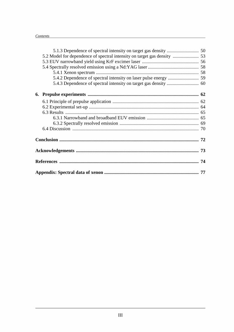
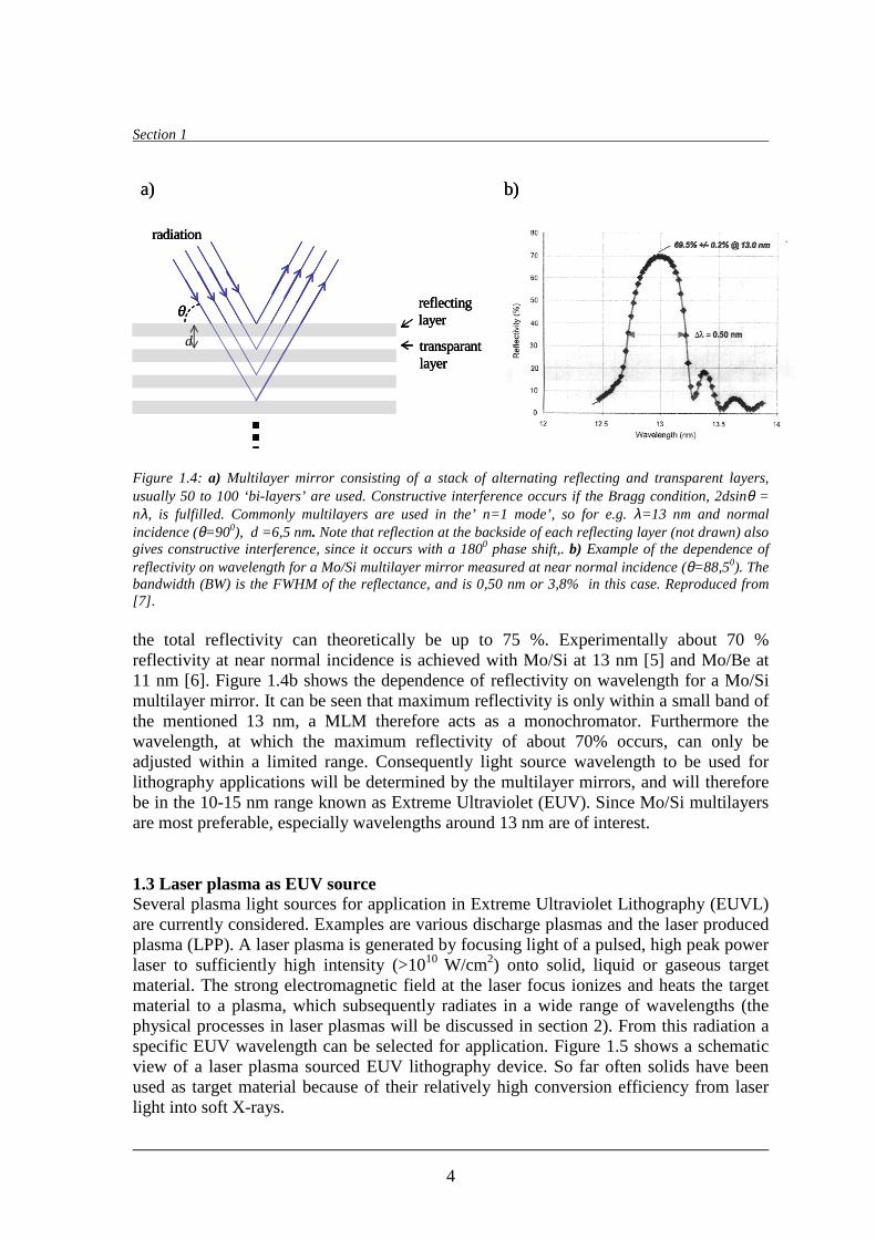
Figure 1.4: a) Multil ayer mirror consisting of a stack of alternating reflecting and transparent layers, usually 50 to 100 ‘bi-layers’ are used. Constructive interference occurs if the Bragg condition, 2dsinθ = nλ, is fulfill ed. Commonly multil ayers are used in the’ n=1 mode’ , so for e.g. λ=13 nm and normal incidence (θ=900), d =6,5 nm. Note that reflection at the backside of each reflecting layer (not drawn) also gives constructive interference, since it occurs with a 1800 phase shift,. b) Example of the dependence of reflectivity on wavelength for a Mo/Si multil ayer mirror measured at near normal incidence (θ=88,50). The bandwidth (BW) is the FWHM of the reflectance, and is 0,50 nm or 3,8% in this case. Reproduced from [7] . the total reflectivity can theoretically be up to 75 %. Experimentally about 70 % reflectivity at near normal incidence is achieved with Mo/Si at 13 nm [5] and Mo/Be at 11 nm [6]. Figure 1.4b shows the dependence of reflectivity on wavelength for a Mo/Si multil ayer mirror. It can be seen that maximum reflectivity is only within a small band of the mentioned 13 nm, a MLM therefore acts as a monochromator. Furthermore the wavelength, at which the maximum reflectivity of about 70% occurs, can only be adjusted within a limited range. Consequently light source wavelength to be used for lithography applications will be determined by the multil ayer mirrors, and will t herefore be in the 10-15 nm range known as Extreme Ultraviolet (EUV). Since Mo/Si multilayers are most preferable, especially wavelengths around 13 nm are of interest. 1.3 Laser plasma as EUV source Several plasma light sources for application in Extreme Ultraviolet Lithography (EUVL) are currently considered. Examples are various discharge plasmas and the laser produced plasma (LPP). A laser plasma is generated by focusing light of a pulsed, high peak power laser to suff iciently high intensity (>1010 W/cm2) onto solid, liquid or gaseous target material. The strong electromagnetic field at the laser focus ionizes and heats the target material to a plasma, which subsequently radiates in a wide range of wavelengths (the physical processes in laser plasmas will be discussed in section 2). From this radiation a specific EUV wavelength can be selected for application. Figure 1.5 shows a schematic view of a laser plasma sourced EUV lithography device. So far often solids have been used as target material because of their relatively high conversion eff iciency from laser light into soft X-rays.

Introduction
5
MLM condenserlaser beamplasma
wafer
MLM demagnifyingoptics
MLM reflection mask
MLM condenserlaser beamplasma
wafer
MLM demagnifyingoptics
MLM reflection mask
Figure 1.5: Schematic view of a lithography device with a laser plasma as EUV source. The specific EUV wavelength is selected by the as monochromator acting multil ayer mirrors. The reflection mask is a multil ayer mirror coated with an absorbing pattern. This pattern is imaged on the wafer by the demagnifying multil ayer optics. However using a solid target laser plasma in a EUV lithography device has two large disadvantages. Firstly ablated material from the target will partly condensate on the optics, and high velocity ions from the plasma can etch the multil ayers, or can even be implanted in the MLM’s up to a depth of several nanometers. This severely affects the performance and li fetime of the MLM optics. The problem of contamination by debris can be reduced by using a fast rotating disc as target in combination with a jet of buffer gas to direct the material away from the optics, see figure 1.6.
fast rotating target
buffer gas
foil trap
laser beam
debris
debris exhaust
radiation (in direction of optics)
fast rotating target
buffer gas
foil trap
laser beam
debris
debris exhaust
radiation (in direction of optics)
Figure 1.6: Debris reduction in a solid target laser plasma. The fast rotating disc target changes the angular velocity distribution of the plasma debris particulates. As result less particulates will move in the direction of the optics. Buffer gas directs the particulates to an exhaust. Furthermore especially small atomic debris is captured on a foil trap by adsorption. Thermalization of the debris atoms is provided by multiple colli sions with buffer gas atoms. This increases the chance that a debris atom colli des with- and sticks to the foil .
Section 1
6
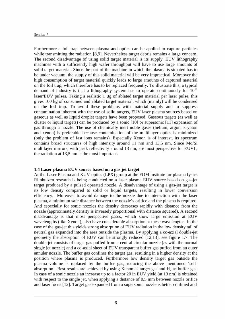
Furthermore a foil trap between plasma and optics can be applied to capture particles while transmitting the radiation [8,9]. Nevertheless target debris remains a large concern. The second disadvantage of using solid target material is its supply. EUV lithography machines with a suff iciently high wafer throughput will have to use large amounts of solid target material. Since the part of the machine in which the plasma is situated has to be under vacuum, the supply of this solid material will be very impractical. Moreover the high consumption of target material quickly leads to large amounts of captured material on the foil trap, which therefore has to be replaced frequently. To ill ustrate this, a typical demand of industry is that a lithography system has to operate continuously for 1011 laser/EUV pulses. Taking a realistic 1 µg of ablated target material per laser pulse, this gives 100 kg of consumed and ablated target material, which (mainly) will be condensed on the foil trap. To avoid these problems with material supply and to suppress contamination inherent with the use of solid targets, EUV laser plasma sources based on gaseous as well as liquid droplet targets have been proposed. Gaseous targets (as well as cluster or liquid targets) can be produced by a sonic [10] or supersonic [11] expansion of gas through a nozzle. The use of chemically inert noble gases (helium, argon, krypton and xenon) is preferable because contamination of the multilayer optics is minimized (only the problem of fast ions remains). Especially Xenon is of interest, its spectrum contains broad structures of high intensity around 11 nm and 13,5 nm. Since Mo/Si multil ayer mirrors, with peak reflectivity around 13 nm, are most perspective for EUVL, the radiation at 13,5 nm is the most important. 1.4 Laser plasma EUV source based on a gas jet target At the Laser Plasma and XUV-optics (LPX) group at the FOM institute for plasma fysics Rijnhuizen research is being conducted on a laser plasma EUV source based on gas-jet target produced by a pulsed operated nozzle. A disadvantage of using a gas-jet target is its low density compared to solid or liquid targets, resulting in lower conversion eff iciency. Moreover to avoid damage to the nozzle due to interaction with the laser plasma, a minimum safe distance between the nozzle’s orifice and the plasma is required. And especially for sonic nozzles the density decreases rapidly with distance from the nozzle (approximately density is inversely proportional with distance squared). A second disadvantage is that most perspective gases, which show large emission at EUV wavelengths (li ke Xenon), also have considerable absorption at these wavelengths. In the case of the gas-jet this yields strong absorption of EUV radiation in the low density tail of neutral gas expanded into the area outside the plasma. By applying a co-axial double-jet geometry the absorption of EUV can be strongly reduced [12,13], see figure 1.7. The double-jet consists of target gas puffed from a central circular nozzle (as with the normal single jet nozzle) and a co-axial sheet of EUV transparent buffer gas puffed from an outer annular nozzle. The buffer gas confines the target gas, resulting in a higher density at the position where plasma is produced. Furthermore low density target gas outside the plasma volume is replaced by the buffer gas, reducing the above mentioned ‘self-absorption’ . Best results are achieved by using Xenon as target gas and H2 as buffer gas. In case of a sonic nozzle an increase up to a factor 20 in EUV yield (at 13 nm) is obtained with respect to the single jet, when applying a distance of 0,5 mm between nozzle orifice and laser focus [12]. Target gas expanded from a supersonic nozzle is better confined and

Introduction
7
laser beam
target gas (e.g. Xe)
a)
buffer gas(e.g. H2)
laser beam
target gas (e.g. Xe)
b)
laser beam
target gas (e.g. Xe)
a)
buffer gas(e.g. H2)
laser beam
target gas (e.g. Xe)
b)
Figure 1.7: Schematic drawings of gas expansions from a single sonic nozzle (a), and a double co-axial sonic nozzle (b). In case of the double nozzle buffer gas is applied to confine the target gas and to ‘blow away’ low density EUV absorbing regions of target gas. This results in higher EUV yield. shows less decrease in density with increasing distance from the nozzle. Furthermore the density gradient at the gas jet-vacuum boundary is steeper in the supersonic case, reducing EUV ‘self-absorption’ . Therefore the effect of applying buffer gas with a supersonic nozzle is less than with the sonic nozzle. An increase in EUV yield up to a factor of 5 can be achieved. 1.5 Report outline This report discusses three different experiments performed with a supersonic xenon gas jet laser plasma EUV source. Section 3 treats backlighting experiments. In these experiments the (initial) neutral xenon gas mass density profile in the supersonic jet is determined by using an absorption technique; keV radiation from a solid target laser plasma is imaged after passing through the jet. Since the radiation is partly absorbed by the neutral xenon a shadowgraph is obtained. From this shadowgraph of the jet the density profile can be constructed. In order to optimize the conversion eff iciency, understanding of the relevant processes in the xenon gas jet EUV source is needed. Therefore spectrally resolved EUV emission from the xenon plasma is studied in section 5 for different laser intensities and initial target gas densities (known from section 3). A simple theoretical model, describing the dependence of spectral intensity on initial target gas density, is presented. The model separately quantifies the dependence of spectral intensity (directly) from the plasma on initial target gas density and the dependence of EUV absorption by neutral xenon surrounding the plasma volume on initial target gas density. Although no experiments with buffer gas are performed, the model can in principal also be used to separately quantify the two effects of using buffer gas, namely an increase in initial target gas density and a reduction of EUV ‘self’ - absorption in the jet, which result in a higher EUV yield, as discussed in section 1.4. Section 6 discusses experiments aimed at increasing the EUV conversion eff iciency of the xenon laser plasma by using a double laser pulse scheme; a laser prepulse is used to adjust the target conditions for the subsequent main pulse. Section 4 gives an overview of the EUV diagnostics used in the experiments of sections 5 and 6. Section 2 deals with theory concerning laser plasmas.

Section 2: Laser plasma processes
8
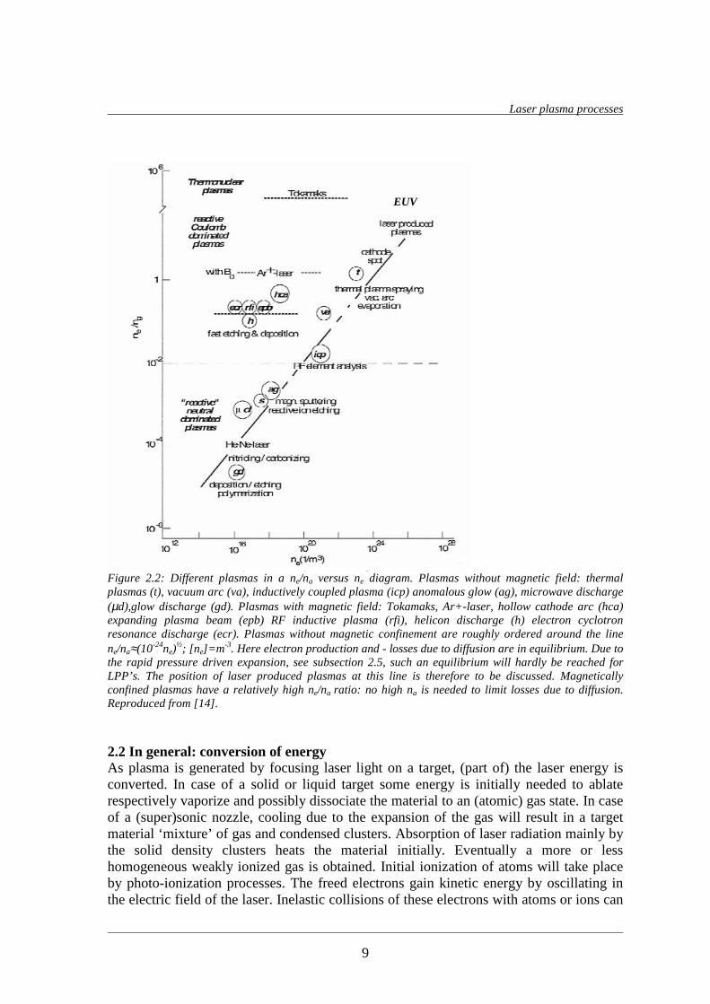
2. Laser plasma processes In this section some characteristics of- and main physical processes in laser produced plasmas will be discussed. Subsection 2.1 discusses the general characteristics of EUV emitting laser produced plasmas in terms of temperature and density compared to other plasmas. Subsections 2.2 to 2.6 discuss the physical processes concerning laser plasmas. 2.1 EUV laser plasma characteristics The discharge- and laser generated plasmas, which are currently considered as EUV source, are rather dense and hot compared to most other plasmas. Figure 2.1 shows various plasmas in a graph of electron density ne versus electron temperature Te, the two most important parameters for any plasma. Figure 2.2 shows different plasmas in a graph of ne/na versus ne, where na is the density of neutrals. EUV/soft X-ray laser produced plasmas typically have ne = 1025 m-3 to 1027 m-3, and Te = 10 eV to 102 eV. Note that when assuming EUV plasma to be a blackbody radiator, see subsection 2.6.5 below, a maximum in intensity around 13 nm wavelength yields a temperature of about 19 eV, cf. figure 2.5c. Practically all atoms are ionized to relatively high stages in EUV emitting (laser) plasmas. Xenon has to be ionized to Xe10+ for high emission at a wavelength of 13,5 nm, see Appendix.
Te (K)
n e(m
-3)
EUV
Te (K)
n e(m
-3)
Te (K)
n e(m
-3)
EUV
Figure 2.1:Different plasmas (artifical and natural) in a ne versus Te diagram. Also pressure as well as Debye length are indicated. Reproduced from [14] .
Laser plasma processes
9
EUVEUVEUV
Figure 2.2: Different plasmas in a ne/na versus ne diagram. Plasmas without magnetic field: thermal plasmas (t), vacuum arc (va), inductively coupled plasma (icp) anomalous glow (ag), microwave discharge (µd),glow discharge (gd). Plasmas with magnetic field: Tokamaks, Ar+-laser, hollow cathode arc (hca) expanding plasma beam (epb) RF inductive plasma (rfi), helicon discharge (h) electron cyclotron resonance discharge (ecr). Plasmas without magnetic confinement are roughly ordered around the line ne/na≈(10-24ne)
½; [ne] =m-3. Here electron production and - losses due to diffusion are in equili brium. Due to the rapid pressure driven expansion, see subsection 2.5, such an equili brium will hardly be reached for LPP’s. The position of laser produced plasmas at this line is therefore to be discussed. Magnetically confined plasmas have a relatively high ne/na ratio: no high na is needed to limit losses due to diffusion. Reproduced from [14] . 2.2 In general: conversion of energy As plasma is generated by focusing laser light on a target, (part of) the laser energy is converted. In case of a solid or liquid target some energy is initially needed to ablate respectively vaporize and possibly dissociate the material to an (atomic) gas state. In case of a (super)sonic nozzle, cooling due to the expansion of the gas will result in a target material ‘mixture’ of gas and condensed clusters. Absorption of laser radiation mainly by the solid density clusters heats the material initially. Eventually a more or less homogeneous weakly ionized gas is obtained. Initial ionization of atoms will t ake place by photo-ionization processes. The freed electrons gain kinetic energy by oscill ating in the electric field of the laser. Inelastic colli sions of these electrons with atoms or ions can

Section 2
10
cause further ionization. Since each ionization produces an extra electron, which in its turn can cause a subsequent ionization, a cascade or avalanche behaviour occurs. The oscill ating electrons can also elastically colli de with ions. The electrons’ kinetic energy is then converted into thermal energy. This process of plasma heating by (laser) radiation is known as inverse Bremsstrahlung. Expansion of the plasma governed by the gigantic pressure gradient yields that part of the thermal energy is converted again into ordered kinetic energy of particles, the plasma therefore cools. Furthermore additional cooling takes place by several radiation processes. Ionization, heating, expansion and radiation processes will be discussed in more detail i n the following subsections. It has to be noted that especially with so-called mass-limited targets, such as liquid droplets, gaseous targets and thin solid films, possibly part of the laser energy is transmitted through the plasma without being absorbed at all . Furthermore in case of high electron densities (especially the case with solid targets), laser light may be reflected where the criti cal density is reached. For laser plasma EUV sources the conversion eff iciency (CE) of laser light into EUV radiation is a key parameter. It is defined as:
laser
EUV
E
ECE =
⋅ BWsr %2
%
π (2.1)
where Elaser is the total energy of the laser pulse and EEUV is the total energy of the EUV pulse at a specific wavelength within a certain bandwidth (BW). The bandwidth is determined by the used multil ayer mirrors, cf. figure 1.4b, and is typically about 4%. As the plasma radiates in all directions the EUV yield is usually given in a maximum collection angle of 2π sr (semi-sphere). The CE for a certain EUV wavelength is therefore expressed in % /(2π sr %BW) as indicated. Note that when multiple MLMs are used in series, as in the optical system of a EUV lithography device, the bandwidth decreases. Typically a BW of 2 % is given for EUVL optical systems, which consist of about 10 multil ayer mirrors. 2.3 Photo-ionization Initial ionization of laser plasma target material takes place by photo-ionization processes. This means that laser radiation directly ionizes the material. If the intensity of the laser radiation is high enough an atom is ionized by absorbing several photons, this process is called multiphoton ionization [16]. For higher intensities tunnel ionization becomes dominant [19], in this process the strong electric field of the laser is able to tilt the atomic potential energy of the electron, enabling it to tunnel ‘out of the atom’ . Multiphoton ionization and tunneling will be discussed in more detail below. 2.3.1 Multiphoton ionization (MPI) The energy of a photon is given by:
λ
ν hchEphoton == (2.2)

Laser plasma processes
11
with h Plank’s constant, ν and λ the frequency respectively wavelength of the radiation and c the speed of light. For laser light with wavelength of 200 nm to 1000 nm the photon energy is about 5 eV to 1 eV. However the ionization potential of e.g. a xenon atom is 12,13 eV [15]. Therefore the ionization can not be a single photon act. However at very high radiation intensities [Wm-2], or photon fluxes [photons⋅s-1m-2], ionization takes place by simultaneous absorption of several photons. This effect is known as multiphoton ionization (MPI). In the MPI process an atom can absorb a photon to create a virtually excited state. The li fetime ∆t of this virtual state is limited by Heisenberg’s uncertainty principle:
ν1
=≤∆photonE
ht (2.3)
For radiation with photon energy of several eV’s ∆t typically is in the order of 10-15 s. If the excited atom is able to absorb a second photon during this brief time interval, it can reach a next virtual state of higher energy with li fe time ∆t≤ 1/2ν. Subsequently a third photon may be absorbed, and so on. By the successive absorption of photons into intermediate virtual states of increasingly higher energy and shorter li fetimes the state of ionization can be reached eventually. The MPI process is schematically shown in figure 2.3a. The probabili ty per unit time for ionization (ionization frequency) of an atom by MPI can be given by [16]: kk
MPI IAAF '==ν (2.4) where F and I are the photon flux and radiation intensity respectively, related by I=EphotonF, and k is the first integer larger than Ei/Ephoton, with Ei the ionization energy. The coeff icients A and A’ depend on atomic species, radiation wavelength and laser light polarization. In idealized and simplest form A respectively A’ can be expressed as:
r r
E(r)E E
a) b)
bound state
r r
E(r)E E
a) b)
bound state
Figure 2.3: Photo-ionization processes. The atomic potential energy is shown as function of distance r from the nucleus, an electron is in a bound state; a) Multiphoton ionization: ionization occurs by the absorption of several photons. b) Tunneling: the electric field of the laser radiation is strong enough to tilt the potential energy, ionization occurs by tunneling through (or even over) the reduced energy barr ier.

Section 2
12
)!1(1 −= − k
Ak
kMPI
νσ
(2.5a)
and:
)!1(
'12 −
== − khE
AA
kk
kMPI
kphoton
νσ
(2.5b)
where σMPI is the cross section for photon absorption into a virtual state. The dependence of the multiphoton ionization frequency νMPI on photon flux F, as given in equation (2.4), can intuitively be understood by the fact that if F increases by e.g. a factor 2, the probabili ty per unit time of each photon absorption also increases by a factor 2. The total probabili ty per unit time of absorption of the required k photons, and thus ionization frequency, then increases by a factor 2k. It is clear that the ionization rate strongly depends on radiation intensity. The longer the radiation wavelength (lower photon energy), the larger k, thus the stronger this dependence will be. Furthermore atoms with lower ionization energy and/or radiation with shorter wavelength yield smaller k values. This results in higher ionization frequency at the same radiation intensity. As an indication table 2.1 shows multiphoton ionization times τMPI for argon at different laser wavelengths and intensities. The ionization time is the inverse of ionization frequency: τMPI =νMPI
-1. Finally it should be noted that if an atomic energy level is in resonance with the photon energy, so that (e.g.) one photon is absorbed into an allowed excited state instead of a virtual state, the multiphoton ionization frequency is strongly enhanced [18]. Table 2.1: Theoretical multiphoton ionization times τMPI=1/νMPI
-1 for argon at different radiation
wavelengths λ and intensities I. The dependence on intensity is in agreement with equation (2.4). Reproduced from [17] .
I (Wcm-2) λ (nm) 5⋅1013 1014 K
586 2 ns 25 ps 6,3 520 1,1 ns 16 ps 6,1 350 0,1 ns 5 ps 4,3
2.3.2 Tunneling As the intensity of the laser radiation increases ionization will occur by tunneling rather than by MPI [19]. In this situation the bound states of the atom shift significantly in energy due to the electric field of the laser radiation. This energy shift, known as AC-Stark shift, is the highest for the bound states. The shift of the Rydberg states and the continuum states of the atom (most weakly bound) approximately equals the ponderomotive energy, given by:
2
20
2
4 ωe
p m
EeE = (2.6)
which is the cycle-averaged kinetic energy of a free electron oscill ating in the electric

Laser plasma processes
13
field of the laser; me and e are the electron mass and charge respectively, E0 is the amplitude of the oscil lating electric field, E=E0sin(ωt), with ω =2πν the angular frequency of the laser radiation. E0 is related to the radiation intensity I by Poynting’s theorem:
2002
1ncEI ε= (2.7)
with ε0 the permittivity of vacuum and n the refractive index. If, by increasing the intensity, the ponderomotive energy approaches the ionization potential Ei of the atom such that:
ip EE2
1> (2.8)
ionization by tunneling becomes dominant. The electric field then becomes strong enough to tilt the atomic potential energy and a potential barrier through which the electron can tunnel (or even escape over) is created. The process of tunneling is shown schematically in figure 2.3b. Note that equation (2.8) is equal to the classical virial theorem, which states that a kinetic energy equal to half the potential energy has to be added to free the electron. Using the equations above with Ei = 10 eV and e.g λ = 248 nm, I has to be in the order of 1015 Wcm-2 for tunneling to become significant. Note that since the ponderomotive energy increases with increasing wavelength (cf. equation (2.6)), the required intensity decreases for longer wavelengths. An estimate for the ion charge Z that can be obtained by tunneling ionization is given by the threshold intensity:
2
41,92 ][ˆ
104][Z
eVEWcmI zi
th−− ⋅= (2.9)
needed to completely suppress the potential barrier, assuming that no ionization occurs
before the barrier is suppressed. 1,ˆ
−ZiE is the ionization potential from Z-1 to Z, and is
given in electronvolts. 2.4 Laser-plasma coupling The electrons freed by photo-ionization processes, described above, gain kinetic energy by oscill ating in the electric field of the laser. Inelastic colli sions between these electrons and atoms or ions result in a further cascade of ionization. Elastic colli sions with ions yield conversion of the electrons’ kinetic energy into thermal energy of the plasma. This process of plasma heating by (laser) radiation is known as inverse Bremsstrahlung. The energy coupling from the electromagnetic field of the laser to the plasma will now be discussed in more detail . Since the ions have much larger mass than the electrons the interaction of the electromagnetic field with the ions can be neglected with respect to the interaction with the electrons. The electrons’ equation of motion in the electromagnetic field is:
Section 2
14
eeehe
e vmEedt
vdm
&
&
&
ν−−= (2.10)
with ev
&
the electron velocity, νeh the electron-heavy particle colli sion frequency for
momentum transfer andE&
the electric field of the laser. (2.10) equates the temporal change of the electrons’ momentum (left hand side) to the electric field force and the resistive force due to colli sions with heavy particles (first respectively second term of
right-hand side). Since the electric field is harmonic, )exp( tiE ω∝&
, and thus also the electron velocity is harmonic, equation (2.10) gives:
)( ων im
Eev
ehee +
−=&
&
(2.11)
The current density due to the movement of the electrons is:
EvenJ ee
&
&
&
σ=−= (2.12)
with σ the conductivity. Combining (2.11) and (2.12) yields:
)(
2
ωνσ
im
ne
ehe
e
+= (2.13)
The real and imaginary components of this complex conductivity are:
22
2
)Re(ων
νσ
+=
eh
eh
e
e
m
ne resp.
22
2
)Im(ων
ωσ+
−=ehe
e
m
ne (2.14)
For the electric- and magnetic fieldE
&
respectively H&
the Maxwell equations hold:
0ε
ρqE =⋅∇&
0)( 0 =⋅∇ H&
µ
t
HE
∂∂
−=×∇)( 0
&
& µ J
t
EH
&
&
&
+∂∂=×∇ 0ε (2.15)
where ρq is the charge density, and ε0 and µ0 are the permittivity respectively permeabili ty of vacuum. Using the complex algebra for E
&
and H&
, such that
))exp(Re()( 0 tiEtE ω&&
= and ))exp(Re()( 0 tiHtH ω&&
= , with 0E&
and 0H&
the ampli tudes of the field, the Maxwell equations can be written as:
0)( =⋅∇ Ep
&
ε 0)( 0 =⋅∇ H&
µ

Laser plasma processes
15
HiE&&
0ωµ−=×∇ EiH p
&&
εωε 0=×∇ (2.16)
where equation (2.12) and a harmonic form of ρq is used: ∂ρq /∂t= iωρq. Furthermore the relative (plasma) permittivity εp is introduced:
0
1ωεσε
ip += (2.17)
Using (2.13) εp can be written as:
+−=
+
+−=
ων
χω
ννω
ωε eheh
eh
pep ii 1111
22
2
(2.18)
where ωpe is the electron plasma frequency:
0
2
εω
e
epe m
en= (2.19)
and χ is:
22
2
ωνω
χ+
=eh
pe (2.20)
The speed of light in vacuum is c=1/√(ε0µ0), and the speed of light in a medium is c/n= √(εpε0µ0), with n the refractive index. The real refractive index is therefore:
22 )()1()1(2
1Re~
ων
χχχε ehprn +−+−== (2.21)
where the equali ty Re(√z)=√(½Re(z)+½|z|) and equation (2.18) are used. In absence of colli sions between electrons and heavy particles, νeh=0, the conductivity is a pure imaginary number, cf. equation (2.13), and the relative permittivity is a pure real number, cf. equation (2.17). The plasma then behaves as a medium without losses, the electronic movement being an orderly oscill ation with a π/2 phase shift with respect to the electric field. In this case there is no energy transfer from the laser field to the plasma, and the field is not damped. However in presence of colli sions, νeh≠0, the conductivity and relative permittivity are not pure imaginary respectively pure real. The orderly oscill ation of the electrons with respect to the field is broken up (shift ≠π/2) due to the colli sions with heavy particles. Energy will flow from the electromagnetic field of the laser to the electrons and from the electrons to the rest of the plasma. The associated time-averaged power dissipation per unit volume in the plasma is:
Section 2
16
22
20
22
0 2
1)Re(
2
1)()(
ωνν
σ+
==⟩⋅⟨=eh
eh
e
edis m
EneEtJtEP
&&
(2.22)
where Re(σ) is given by (2.14). Note that )(tE&
and )(tJ&
are both real, with
))exp(Re()( 0 tiEtJ ωσ&&
= , where σ is complex, cf. equation (2.13). The dissipated power
can be used for ionization in case of inelastic colli sions between electrons and atoms or ions, a cascade or avalanche effect of ionization then occurs [16]. Elastic colli sions between electrons and ions yield that the dissipated power is used for plasma heating, thus thermal motion of ions and electrons [20]. Although elastic and inelastic colli sions generally take place at the same time, the effect of both colli sion types will be discussed separately. Subsection 2.4.1 deals with cascade ionization, which is especially important in the starting phase of the plasma. Subsection 2.4.2 discusses inverse Bremsstrahlung heating. 2.4.1 Cascade Ionization As an ill ustration only colli sional ionization of neutral atoms to single charged ions is considered. This is the case when the plasma is still weakly ionized. The dissipated power Pci in the plasma is given by equation (2.22), where in this case νeh=νea, with νea the colli sion frequency for electron-atom momentum transfer:
)(2
122
20
2
ωνν
+=
ea
ea
e
eci m
EneP (2.23)
If the dissipated power is entirely used for ionization the following energy balance holds:
cii
i Pdt
dnE = (2.24)
with ni the ion density, and Ei the ionization potential. The left hand side of the equation represents the power density involved with the ion production. Since only single ionization is considered ni=ne and dne/dt=dni/dt. Combining this with equations (2.23) and (2.24) gives for the time dependence of electron and ion density:
⋅
+== t
Em
Eentntn
ea
ea
ieie
)(2
1exp)()(
22
20
2
0 ωνν
(2.25)
with n0 the initial electron and ion density at t=0. Note that E0 is in V/m, whereas Ei is in joule. The exponent in equation (2.25) clearly reflects the avalanche or cascade behaviour of the ionization process. The colli sion frequency νea is given by [14]:
1310
ˆ
ea
eaea C
Tn≈ν 10ˆ1,0 << eT eV (2.26a)
Laser plasma processes
17
ea
aea K
n≈ν 10ˆ >eT eV (2.26b)
where Cea and Kea are factors depending on atomic species, na is the density of neutral
atoms, and eT is the electron temperature in electronvolts: eT =kBTe/e with kB Boltzmann’s
constant and Te in Kelvin. E.g. for argon Cea = 3,5 m-3eV· s and Kea = 3⋅1012 m-3s (no data for xenon is found). For the supersonic gas jet under study the initial gas density na is in the order of 1025 m-3 (cf. section 3). For argon νea is then in the order of 1011-1012 s-1. For laser light in the wavelength range 200-1000 nm, ω is in the order of 1015 s-1. Thus ω >>νea is generally the case in this study. This condition implies that the factor νea /( νea
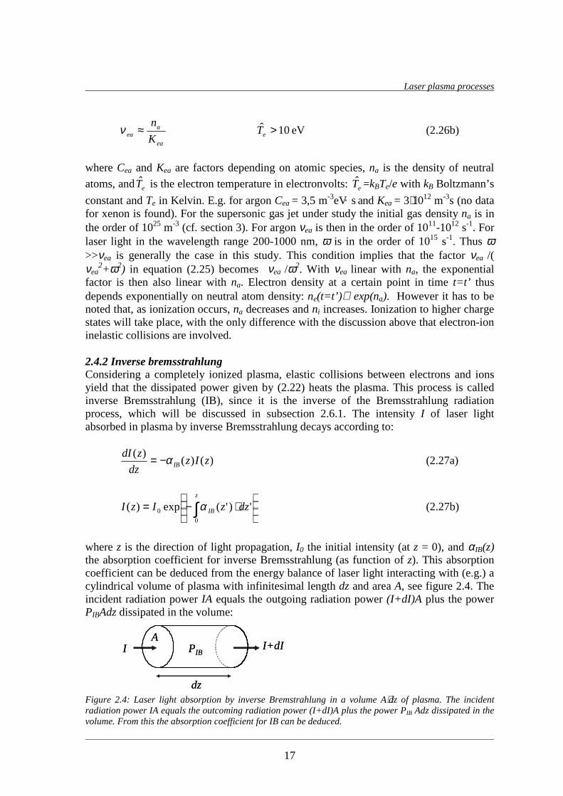
2+ω2) in equation (2.25) becomes νea /ω2. With νea linear with na, the exponential factor is then also linear with na. Electron density at a certain point in time t=t’ thus depends exponentially on neutral atom density: ne(t=t’ )∝ exp(na). However it has to be noted that, as ionization occurs, na decreases and ni increases. Ionization to higher charge states will t ake place, with the only difference with the discussion above that electron-ion inelastic colli sions are involved. 2.4.2 Inverse bremsstrahlung Considering a completely ionized plasma, elastic colli sions between electrons and ions yield that the dissipated power given by (2.22) heats the plasma. This process is called inverse Bremsstrahlung (IB), since it is the inverse of the Bremsstrahlung radiation process, which will be discussed in subsection 2.6.1. The intensity I of laser light absorbed in plasma by inverse Bremsstrahlung decays according to:
)()()(
zIzdz
zdIIBα−= (2.27a)
⋅−= ∫
z
IB dzzIzI0
0 ')'(exp)( α (2.27b)
where z is the direction of light propagation, I0 the initial intensity (at z = 0), and αIB(z) the absorption coeff icient for inverse Bremsstrahlung (as function of z). This absorption coeff icient can be deduced from the energy balance of laser light interacting with (e.g.) a cylindrical volume of plasma with infinitesimal length dz and area A, see figure 2.4. The incident radiation power IA equals the outgoing radiation power (I+dI)A plus the power PIBAdz dissipated in the volume:
dz
I PIBI+dI
A
dz
I PIBI+dI
A
Figure 2.4: Laser light absorption by inverse Bremstrahlung in a volume A⋅dz of plasma. The incident radiation power IA equals the outcoming radiation power (I+dI)A plus the power PIB Adz dissipated in the volume. From this the absorption coefficient for IB can be deduced.

Section 2
18
IBIB Pdz
dIAdzPAdIIIA −=⇒++= )( (2.28)
The dissipated power PIB per unit volume is given by equation (2.22), where in this case νeh=νei, with νei the coll ision frequency for electron-ion momentum transfer:
22
20
2
2
1
ωνν
+=
ei
ei
e
eIB m
EneP (2.29)
Combining equations (2.27a) and (2.28) gives:
)(~ 22
2
ωννω
α+
==ei
ei
r
peIBIB cnI
P (2.30)
where equation (2.7) is used to relate the laser intensity I to the amplitude E0 of the electric field. The electron plasma frequency ωpe and real refractive index rn~ are as given
in equation (2.19) and (2.21) respectively. With the conditions ω >>ωpe and ω >>νei,, which generally apply for the plasmas under study, equations (2.20) and (2.21) give
2)/(1~ ωω pern −= ce nn /1−= , with nc the criti cal density (at which ωpe=ω in
equation (2.19)) given by:
2
20
e
mn e
c
ωε= (2.31a)
][1012,1][ 2153 mmnc
−− ⋅⋅= λ (2.31b)
Furthermore νei
2 can be neglected with respect to ω2
in the denominator of the second factor in the right hand side of equation (2.30). By substituting νei, ωpe, and rn~ in equation (2.30), the absorption coefficient for inverse Bremsstrahlung can then be written as [1, p133] [21]:
2/3
2
*2
5
ˆ1
1
ln1008,1
e
c
ec
eIB
T
n
nn
nZ
−
Λ
⋅⋅=
−
λα (2.32)
where Z* is the average ion charge, and lnΛ the coulomb logarithm:
=Λ
e
eBeB
ne
Tk
Ze
Tk2
02
043lnln
επε (2.33a)
Laser plasma processes
19
⋅=Λ
2/1
2/313
ˆ1055,1lnln
e
e
Zn
T (2.33b)
For laser light with wavelength 200-1000 nm nc is ~ 3· 1028 to 1027 m-3. Therefore ne will be well below the criti cal density nc (which is equal to ωpe << ω) in case of gaseous target laser plasmas. The absorption coeff icient for inverse Bremsstrahlung is then proportional to the electron density squared (neglecting the ne dependence of the Coulomb logarithm). If electron density approaches the criti cal density absorption increases very strongly. In the limi t of ne → nc, or ω → ωpe, resonant energy transfer to a plasma motion takes place. This process referred to as resonant absorption is also described as ‘ the excitation of plasma waves’ . For ne above the criti cal density laser radiation is completely reflected. 2.5 Plasma expansion As soon as plasma is generated it will expand into the surrounding vacuum. A first estimate for the plasma expansion velocity can be given by the ion acoustic velocity [14]:
i
e
i
eBs A
TZ
M
TkZc
ˆ104 ⋅
≈⋅
= (2.34)
where Mi≈Aimp is the ion mass, with Ai the ion mass number (atomic weight) and mp the proton mass. cs is the maximum velocity with which ambipolair diffusion of the plasma can occur. In this process the relatively mobile electrons diffuse out of the plasma more rapidly than the relatively immobile ions. Hence an electric field is created which slows down the electrons and accelerates the ions outwards. So effectively diffusion takes place with the velocity (thus temperature) of the electrons and the inertia (thus mass) of the ions, as can be seen in equation (2.34). However, given the densities ne = O(1026 m-3) and
ni = O(1025 m-3)) and the temperatures ei TT ˆˆ ≤ = O(10 eV), the pressure p in the plasma:
)( eeiiB TnTnkp += (2.35)
will be in the order of 108 Pa. This causes the plasma rather to ‘explode’ into the surrounding vacuum. Thermal energy is then converted into directed kinetic energy. With the acoustic ion speed estimate the expansion velocity of a xenon plasma with Ai= 131,
Z=10 and eT in the order of 10 eV is in the order of 104 m/s. In [22] the pressure driven
expansion velocities are higher than the cs estimate. The expansion of laser generated plasmas leads to a rapid decrease of the electron (and ion) density. This results in less absorption by inverse Bremsstrahlung, equation (2.32). Some time after the generation of the plasma began a considerable part of the laser radiation will t herefore be transmitted. This is especially the case with gaseous targets, where initial density already is relatively low. Hence to obtain high conversion eff iciency laser pulses should not be too long.

Section 2
20
2.6 Radiation In general radiation emitted by plasmas can be divided in continuum- and line radiation. Continuum radiation incorporates Bremsstrahlung (‘brake radiation’) and recombination radiation, both involve an interaction between a free electron and an ion. Line radiation is generated by transitions of electrons between bound (excited) states in an atom or ion. The population of the different excited states must be calculated with a colli sional radiative model. Heavier elements show quasi continuum radiation, consisting of many (unresolvable) close lines. If plasma is optically thick blackbody radiation occurs. The various radiation processes will be discussed in more detail below. 2.6.1 Continuum radiation Bremsstrahlung occurs when an electron elastically colli des with an ion (or atom), its deflection results in generation of radiation. Since a transition between free states of electrons is concerned, this type of radiation is also known as free-free (ff) radiation. For example Bremsstrahlung with a XeZ+ ion: νheXeeXe ZZ ++→+ ++ (2.36) Recombination radiation occurs when an ion with charge Z+ recombines with an electron to an excited state or the ground-state of the resulting ion with charge (Z-1)+. This is associated with a transition from a free electron state into a bound electron state; hence recombination radiation is also called free-bound radiation. Example: νhpXeeXe ZZ +→+ +−+ )()1( (2.37) where p indicates an excited state. The photon energy is minimum the ionization energy of the resulting (excited) ion. This leads to a ‘comb structure’ in the spectrum, see figure 2.5a. The radiation density for continuum radiation (thus free-free electron-ion Bremsstrahlung and free-bound recombination radiation) per unit wavelength and 4π sr solid angle can be given by [20, (2.68)] or [22]:
)),,(),(()(exp233
~),,( 2
22230
6
, ZTGTGZZnTk
hc
Tk
m
cm
ennnTj efbeff
Zi
eBeB
e
e
ereecont λλ
λπλπελλ +
−= ∑
4m
W (2.38)
Where the sum is carried out over the present ionization stages with charge Z and corresponding ion density ni(Z). For the refractive index rn~ equation (2.21) holds, where the wavelength or angular frequency of the continuum radiation has to be substituted. Gff is the Gaunt factor for Bremsstrahlung given by [20, (2.75)]:
=
eBeBeff Tk
hcK
Tk
hcTG
λλπλ
22exp
3),( 0 =
hc
Tk eBπλπ3
for eBTkhc >>λ

Laser plasma processes
21
I→
λ →
a) b)
c)
UTA
λ →
I →
0.0
0.5
1.0
1.5
2.0
2.5
3.0
0 5 10 15 20 25 30 35 40 45 50λ (nm)
I (
1022
Wm
-3)
=19 eVT
=17 eVT
=15 eVT
I→
λ →
I→
λ →
a) b)
c)
UTA
λ →
I →
0.0
0.5
1.0
1.5
2.0
2.5
3.0
0 5 10 15 20 25 30 35 40 45 50λ (nm)
I (
1022
Wm
-3)
=19 eVT=19 eVT
=17 eVT=17 eVT
=15 eVT=15 eVT
Figure 2.5: Appearance of different radiation processes in spectrum: a) Comb structure of continuum recombination radiation. b) Line radiation with Lorentz-profile line broadening. In a wavelength interval containing many close lying transitions, the spectrum becomes unresolved, an unresolved transition array (UTA) can be observed. c) Blackbody radiation, Planck intensity distribution Iλ for three different temperatures T=15 eV, 17 eV and 19 eV, corresponding to wavelength of maximum intensity λmax = 16,7 nm, 14,7 nm and 13,2 nm respectively.
=
hc
Tk
g
eB
γλ
π4
ln3
for eBTkhc <<λ
(2.39)
with K0(x) the modified Bessel function and γg = exp(γe) ≈1,781 with γe ≈ 0.577 Euler’s constant. Gfb is the Gaunt factor for recombination radiation and is given by [22]:
∑
−= −−−
pp
eB
pZip
eB
Ziefb g
Tk
EEgp
Tk
EZTG )(~exp),,( 1,51, λλ (2.40)
where the sum is carried out over all the excited states with principal quantum number p of the ionization stage with charge Z-1. Ei,Z-1 is the ionization energy from Z-1 to Z, gp is the degeneracy of the excited level p and Ep its energy with respect to the ground level of the ion with charge Z-1. )(~ λpg is the Gaunt factor for the related transition (equation
(2.37)). Note that a Maxwelli an electron energy distribution is assumed, which results in the exponent factor in (2.38). From equation (2.38) and (2.39) the following hold for the radiation density due to Bremsstrahlung:

Section 2
22
−∝
eB
eff Tk
hcZnj
λλλ exp2/3
2
, for eBTkhc >>λ
−
⋅∝
eB
eeff Tk
hcTCZnj
λλλ
λ exp)ln(
2
2
, for eBTkhc <<λ
(2.41)
with C constant. For simplicity a single ionization stage with charge Z is considered, and thus ne=niZ. Note that the refractive index, given by equation (2.21), is considered to be constant and equal to unity. This is justified since for EUV wavelengths ω will be much larger than ωpe. It can be calculated that for the EUV wavelength range (λ=10 nm to 20
nm), the condition hc/λ>kBTe is valid for eT < 63eV. Since this will be generally the case
with the laser plasmas under study (cf. figure 2.6), the upper approximation in (2.41) for j ff can be taken. However in both cases of equation (2.41) the free-free radiation density at a specific wavelength is proportional to ne
2Z and increases with temperature Te as exp(-Te
-1). The approximation for hc/λ<<kBTe has an additional (weak) dependence on Te, giving an ‘extra’ increase in radiation density with increasing electron temperature. From equations (2.38) and (2.40) the radiation density j fb for recombination is:
∑∑
−
−∝ −−
−p
peB
pZip
ZZii
eBe
efb g
Tk
EEgpEZn
Tk
hc
T
nj )(~expexp 1,5
1,2
2/32, λλλλ (2.42)
In case a single ionization stage is considered the first sum in the equation can be omitted. Equation (2.42) yields that the free-bound radiation density, li ke free-free radiation density, is proportional to neniZ
2, or ne2Z. Furthermore it also increases with Te
as exp(-Te-1). The first exponential factor in (2.42) gives an increase with increasing Te,
whereas the exponential factor in the (second) sum gives a decrease with increasing Te. However the energy of the emitted photon is minimum the ionization energy of the excited ion resulting from the recombination, or hc/λ ≥ Ei,Z-1-Ep. This means that the radiation density indeed increases exponentially with electron temperature as exp(-Te
-1). Note that the free-bound radiation density also is proportional to Te
-3/2. This yields that the recombination radiation density only increases with electron temperature, ∂j fb/∂Te>0, for (hc/λ)-(Ei,Z-1-Ep)>
3/2kBTe. Note that the fact that Bremsstrahlung- and recombination radiation densities are proportional neniZ
2 can easily be understood, since in both continuum radiation processes electron-ion colli sions are involved. The radiation (power) density will t herefore be proportional to the amount of colli sions per unit volume and time. The electron-ion colli sion frequency is proportional to niZ
2, hence the radiation density is proportional to neniZ
2. 2.6.2 Line radiation Line radiation is generated by electronic transitions between excited states of atoms or ions. Only bound states of electrons are involved, therefore it is also known as bound-bound (bb) radiation. E.g.: pq
ZZ hpXeqXe ν+→ ++ )()( (2.43)
Laser plasma processes
23
with p and q indicating the excited states. Note that in the classification of spectral li nes a neutral atom, e.g. neutral xenon, is often indicated as XeI, single ionized xenon (Xe+) as XeII, and so on. The radiation density of the spectral li ne corresponding with the transition q→ p can be written as:
pqqpqqpbb EAnJ ∆=,
3m
W (2.44)
with np the density of the level p, and ∆Epq=Eq-Ep=hνpq=hc/λpq the difference in energy between level p and q (which is equal to the photon energy of the emitted radiation). Aqp is the related transition probabili ty given by:
2
320
22pq
e
qpqp Echm
efA ∆=
επ
(2.45)
where fqp is the so-called oscill ator strength. The radiation density is thus proportional with the density of the excited level q, which in principal can be calculated by using a colli sional radiative model, see subsection 2.6.3 below. Note that a spectral li ne is broadened by several broadening mechanisms, which will not be discussed here. Figure 2.5b schematically shows a spectrum containing lines, broadened with a Lorentz profile. 2.6.3 Collisional radiative models Both colli sional and radiative ionization, recombination, excitation and de-excitation processes occur in a plasma. If the rates of all these processes are known, the population -thus density- of all i onization stages and their excited levels can be calculated. Usually more simpli fied colli sional radiative models (CRM’s) are used. These models only take into account the most dominant (=fast) processes. As for instance the density of a plasma increases, colli sional processes will become more important than radiative processes. Colli sional ionization is then balanced by three-body recombination: eeXeeXe ZZ ++↔+ +++ )1( (2.46) and colli sional excitation and de-excitation are balanced: eqXeepXe ZZ +↔+ ++ )()( (2.47) In this situation, known as local thermal equil ibrium (LTE), the populations of the ionization stages and their excited levels are thus entirely controlled by electron colli sions, and determined by electron temperature and density. The density of the different ionization stages are interrelated by Saha’s equation [20, (2.57)], the densities of the excited levels within the same ionization stage are interrelated by Boltzmann’s equation [20, (2.56)]. These can be combined to the Saha-Boltzmann equation, giving the density np(Z) of excited level p of ionization stage Z:

Section 2
24
−
++
=eB
pZi
eBe
ie
p
p
Tk
ZEE
Tkm
h
ZQ
Znn
Zg
Zn )(exp
2)1(2
)1(
)(
)( ,
2/32
π (2.48)
gp(Z) is the corresponding statistical weight of excited level p, ni(Z+1) is the total density of the ionization stage Z+1. Ei,Z is the ionization energy from the ground level of Z to the ground level of Z+1. Ep(Z) is the energy of the excited level p of ionization stage Z with respect to the ground level of this ion. Q(Z+1) is the partition function of ion Z+1:
∑+
+−+=+
)1(
)1(exp)1()1(
Zp eB
pp Tk
ZEZgZQ (2.49)
where the sum is carried out over all the excited levels p(Z+1) of ionization stage Z+1, with statistical weights gp(Z+1) and energies Ep(Z+1). For optically thin plasmas (see subsection 2.6.5 ‘blackbody radiation’ below) it is shown that LTE is valid for electron densities [20, (2.59)]:
3max,
2/119 ˆˆ106,8 iee ETn ⋅≥ (LTE) (2.50)
with ne in m-3, eT the electron temperature in eV and max,ˆ
iE the highest ionization energy
in eV of any of the atoms or ions present in the plasma. For optically thick plasmas LTE is already valid at lower electron densities. Furthermore note that in case of LTE electron temperature equals ion temperature: Te=Ti. If electron density is relatively low, radiative processes become more important than colli sional processes. In this case of coronal equili brium, colli sional ionization is balanced by radiative recombination (equation (2.37)), and colli sional excitation is balanced by spontaneous radiative de-excitation (equation (2.43)). Note that excitation by the absorption of a photon is considered to be negligible in case of optically thin plasmas. Since both colli sional ionization and radiative recombination are proportional to the electron density, the relative population of the different ionization stages is independent of electron density [20, (2.60)]:
( )
⋅≅
+−
eB
Zi
eB
Zi
i
i
Tk
E
Tk
E
Zn
Zn ,
4/3
4/11,9 exp
ˆ108
)1(
)( (Coronal Equili brium) (2.51)
From equations (2.48) and (2.51) it is clear that both for LTE and Corona higher ionization stages become more populated with increasing temperature. Furthermore in case of LTE lower ionization stages become relatively more populated than higher ionization stages as electron density increases. Theory and experiments presented in section 3 give an initial gas density in the order of na=1025 m-3 for the xenon target used in this study. With ionization to Xe10+ for optimal EUV emission, this yields that the electron density is in the order of ne=1026 m-3. Since the plasma expands, this number for the electron density actually is a maximum estimate.

Laser plasma processes
25
Equation (2.50) implies that for LTE ne > 2,4· 1026 m-3, where eT ≈ 30 eV (see below) and
max,ˆ
iE ≈80 eV is taken. The plasmas in this study are therefore rather in coronal
equili brium than in LTE. A colli sional radiative model, which lies between the corona- and LTE limit is given by [45]. The dominant ionization stage as a function of electron temperature in a solid xenon target laser plasma calculated with this model is given in [46] and is shown in figure 2.6. It can be seen that Xe10+ as dominant ionization stage yields an electron temperature of 34 eV. Solid xenon target laser plasmas will be closer to LTE than the gaseous xenon target laser plasmas in this study, because of their higher density. Three body recombination, shifting the balance to lower ionization stages, cf. equation (2.46), wil l thus be faster in solid xenon plasmas than in gaseous target plasmas. Therefore in the laser plasmas under study a specific ionization stage will become dominant at a lower electron temperature than indicated in figure 2.6.
0
2
4
6
8
10
12
14
16
18
0 10 20 30 40 50 60 70 80 90 100 110 120Te (eV)
dom
inan
t ion
izat
ion
stag
e
Figure 2.6: Dominant ionization stage as function of electron temperature in a solid xenon target laser plasma according to the model of Colombant and Tonon [45] . Reproduced from [46] . 2.6.4 Quasi continuum radiation Radiative plasmas containing atomic species with a relatively low atomic number ZA show spectra containing well distinguishable lines. As ZA increases the number of possible transitions also increases. Consequently spectra will consist of broadband structures containing many lines. In some wavelength intervals lines may lie so close that they completely overlap (due to line broadening) and merge into a band of quasi continuum radiation up to 1 nm wide. Such a band is called a unresolved transition array (UTA). Xenon is known to have an unresolved transition array in the EUV region at 11 nm [36]. An UTA is shown schematically in figure 2.5b. 2.6.5 Blackbody radiation Besides emission of radiation also absorption takes place in plasmas. Dependent on the amount of absorption a distinction between optically thick and optically thin radiation can be made. For optically thick radiation, absorption is large:

Section 2
26
1),( >>= ∫R
o
drrk λτ (optically thick) (2.52)
where k(λ) is the absorption coeff icient dependent on wavelength and R the plasma radius. In case of thermal equili brium the plasma then acts as a black body surface emitter with temperature T, for which Planck’s intensity distribution holds:
−
=1)exp(
8
5
2
Tk
hc
hcI
Bλλ
πλ
3m
W (2.53)
giving the intensity per unit wavelength (over 4π sr angle). The wavelength of maximum intensity is given by Wien’s law:
13max 109,22.0 −−⋅=≈ T
Tk
hc
B
λ (2.54)
And the total intensity I integrated over λ is given by: 4TI σ= (2.55) with σ Stefan-Boltzmann’s constant. Note that the intensity of radiation at each wavelength from any plasma (optically thick or thin) cannot exceed the value given by the Planck distribution. This distribution thus also indicates a limit i n spectral intensity Iλ. As an example figure 2.5c shows the spectrum of a blackbody emitter at three different temperatures T =15 eV, 17 eV and 19 eV. The corresponding wavelengths of maximum intensity are λmax =16,7 nm, 14,7 nm and 13,2 nm respectively. For optically thin radiation: 1<<τ (optically thin) (2.56) Absorption can be neglected. However for an intermediate case, where τ =O(1), absorption has to be taken into account.
Section 3: Backlighting
27
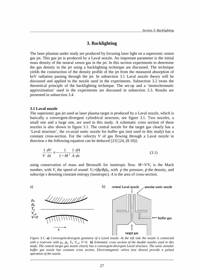
3. Backlighting The laser plasmas under study are produced by focusing laser light on a supersonic xenon gas jet. This gas jet is produced by a Laval nozzle. An important parameter is the initial mass density of the neutral xenon gas in the jet. In this section experiments to determine the gas density in the jet using a backlighting technique are discussed. The technique yields the construction of the density profile of the jet from the measured absorption of keV radiation passing through the jet. In subsection 3.1 Laval nozzle theory will be discussed and applied to the nozzle used in the experiments. Subsection 3.2 treats the theoretical principle of the backlighting technique. The set-up and a ‘monochromatic approximation’ used in the experiments are discussed in subsection 3.3. Results are presented in subsection 3.4. 3.1 Laval nozzle The supersonic gas jet used as laser plasma target is produced by a Laval nozzle, which is basically a convergent-divergent cylindrical structure, see figure 3.1. Two nozzles, a small one and a large one, are used in this study. A schematic cross section of these nozzles is also shown in figure 3.1. The central nozzle for the target gas clearly has a ‘Laval structure’ , the co-axial sonic nozzle for buffer gas (not used in this study) has a constant cross-section. For the velocity V of gas flowing through a Laval nozzle in direction x the following equation can be deduced [23] [24, (8.10)]:
dx
dA
AMdx
dV
V
1
1
112−
−= (3.1)
using conservation of mass and Bernoulli for isentropic flow. M=V/Vs is the Mach number, with Vs the speed of sound: Vs=(∂p/∂ρ)s, with p the pressure, ρ the density, and subscript s denoting constant entropy (isentropic). A is the area of cross-section.
a) b)
p0
ρ0
T0
Vs,0
V=0
x
p0
ρ0
T0
Vs,0
V=0
x Figure 3.1: a) Convergent-divergent geometry of a Laval nozzle. At the left side the nozzle is connected with a reservoir with p0, ρ0, T0, Vs,0, V=0. b) Schematic cross section of the double nozzles used in this study. The central target gas nozzle clearly has a convergent-divergent Laval structure. The sonic annular buffer gas nozzle has constant cross section. Electromagnetic valves (not shown) provide a pulsed operation of the nozzle.
target gas
buffer gas
central Laval nozzle annular sonic nozzle
target gas
buffer gas
central Laval nozzle annular sonic nozzle

Section 3
28
From (3.1) it can be seen that there are several possibiliti es: if the flow through the nozzle is subsonic, M<1, the velocity V will i ncrease with decreasing cross-section area A and vice versa. For supersonic flow, M >1, the velocity V will however increase with increasing cross-section area A, and decrease with decreasing area. M=1 gives a singularity in (3.1), and is only possible at the throat of the nozzle where A is minimum and dA/dx=0. In practice one side of the nozzle is connected to a gas bottle, i.e. a reservoir of gas with p=p0, ρ=ρ0, V=0, Vs=Vs,0 and temperature T=T0. When the pressure at the opposite exit side of the nozzle is (slightly) smaller than p0, gas will flow through the nozzle. In first instance the flow will be subsonic, M<1, everywhere in the nozzle. When the pressure at the exit side is further decreased the velocity of the flow wil l increase everywhere in the nozzle. Eventually the Mach number at the throat becomes 1, while everywhere else still M<1. This situation is known as choking, since the velocity and Mach number at the throat cannot be increased anymore. If namely the Mach number at the throat would be larger than one, this would mean that there is a transition from M<1 to M>1, and that consequently M=1, at a position in front of the throat. However as stated above the situation M=1 is only possible at the throat. Nevertheless lowering pressure at the exit side even more in case of choking does result in a transition from subsonic to supersonic flow at the throat. The flow in the divergent part of the nozzle then becomes supersonic instead of subsonic. So lowering pressure at the exit of the nozzle will continuously increase the velocity and Mach number throughout the nozzle until choking is reached. Lowering the pressure even more results in a further increase in velocity and Mach number in the divergent part of the nozzle, where a supersonic flow is then established. Figure 3.2 shows the dependence of the Mach number as function of position in the nozzle as discussed. M, p, ρ, T and Vs are coupled by the isentropic relations for a perfect gas [23]:
1
1
21
2
0,
1
1
0
1
00 2
11
−−−−
−+=
=
=
=
γγγγ γρρ
MV
V
T
T
p
p
s
s (3.2)
where γ = cp/cv, with cp and cv the specific heat of the gas at constant pressure and constant mass density respectively. In case of choking the mach number M at certain point x with cross-section area A can be found by using equation (3.2) and conservation of mass, ρVA = constant:
)1(2
1
2
2
11
1
21 −+
−+⋅
+
=γ
γ
γγ
MMA
A
th
(3.3)
with Ath the cross-section area at the throat. Equation (3.3) has two solutions for M, namely the subsonic one, M < 1, and the supersonic one, M > 1. At the throat, with area Ath, M =1. The small nozzle used in this study has a diameter at the throat of 0,15 mm, the diameter at the exit of the nozzle is 0,41 mm. The large nozzle has a throat diameter of 0,33 mm and an exit diameter of 1,14 mm.

Backlighting
29
0
xthroat exit
1
M
reservoir0
xthroat exit
1
M
reservoir
Figure 3.2: Mach number M as function of position x in the nozzle for different situations. The two lower graphs represent situations in which the flow is subsonic throughout the nozzle, and where choking does not occur. The upper graph is the situation of choking, M=1 at the throat. The flow in the divergent part of the nozzle has two (isentropic) solutions in this case: subsonic (lower branch) and supersonic (upper branch). Note that a Mach number lower than given by the supersonic branch can be established by a non-isentropic shock. Examples of two shocks are given by the two dotted lines originating from the upper supersonic branch. The Mach number at the exit of the nozzles Mexit, can thus be found by substituting A/Ath=(0,41/0,15)2=7,5 for the small nozzle and A/Ath=(1,14/0,33)2=11,9 for the large nozzle in the left hand side of (3.3). For xenon with γ=5/3 the result is Mexit=4,5 and Mexit=5,4 for the small and large nozzle respectively. Note that, because pressure difference between reservoir and exit will be suff iciently high, the supersonic solution can be taken. In practice the ‘backing pressure’ pback=p0 in the reservoir can be measured. For an ideal gas the following equation holds:
00 Tk
pM
B
backat=ρ (3.4)
where Mat is the mass of the gas atom or –molecule [kg] and kB Boltzmann’s constant. Combining the results for Mexit with eqs. (3.2) and (3.4) gives the density at the nozzle exit ρexit for xenon: ][25,0][ 3 barpkgm backexit ⋅=−ρ (small nozzle) (3.5a)
][15,0][ 3 barpkgm backexit ⋅=−ρ (large nozzle) (3.5b)
where Mat = 2,19· 10-25 kg, T0 = 293 K and 1 bar = 105 Pa is used. For xenon a mass density of ρ = 1 kg/m3 corresponds to a particle density of na = 4,6· 1024 m-3. With pback in the order of 10 bar the mass density ρ will be in the order of 1 kg/m3, and na in the order of 1025 m-3. It has to be noted that temperature at the nozzle exit in this case is T = 33 K,

Section 3
30
according to equation (3.2). The boili ng point of xenon is at 166 K, so clearly a supersaturated state is reached and cluster formation will t ake place. This complicates the physics of the Laval nozzle described above. 3.2 Backlighting principle With the backlighting technique the mass density profile of gas in the jet can be determined from the absorption of radiation passing through the jet. This will be discussed in the following. Absorption by the neutral gas leads to attenuation of radiation passing through the jet, according to:
)()()( λλλ
Ikdy
dIa ⋅−= (3.6)
with I(λ) the (spectral) intensity of the radiation propagating in the y-direction and ka(λ) the absorption coeff icient. This absorption coeff icient depends on the mass density ρ of the gas by: ρλκλ ⋅= )()(ak (3.7)
with κ(λ) [kg-1m2] the specific absorption coeff icient of the gas, which is only dependent on the wavelength of the radiation. Assuming a radially symmetric mass density in the jet, ρ(r), the intensity I(x) of monochromatic radiation passed through the jet at position x, see figure 3.3, is given by:
−⋅= ∫
=
0
0
0 )(2exp)()(y
y
dyrxIxI κρ (3.8)
with I0(x) the initial intensity at position x. For κ the value at the specific wavelength of the monochromatic radiation has to be taken. Using x2+y2=r2 and x2+y0
2=R2, where R is the radius of the jet, the integral in equation (3.8) can be rewritten:
x R
y0
I(x)I0(x)x R
y0
I(x)I0(x)
Figure 3.3: Schematic cross-section of the gas-jet. From the absorption of radiation by the neutral gas the gas mass density as function of radius can be determined by using an inverse Abel transform.

Backlighting
31
−−⋅= ∫
=
R
xr xr
rdrrxIxI
220
)(2exp)()(
κρ (3.9)
Defining P(x) as:
∫= −
=
=
R
xr xr
rdrr
xI
xIxP
22
0 )(2
)(
)(ln)(
κρ (3.10)
ρ(r) can be found by using the inverse Abel transform [25,26]:
( )
dxrx
dxxdPr
R
rx∫= −
−=22
/)(1)(
πκρ (3.11)
Note that P(x) actually is the integrated absorption coeff icient at position x. In practice P(x) can be measured. However due to noise the curve of P(x) will not be smooth so that the derivative dP(x)/dx generally cannot be determined (numerically) from the data. By applying a curve-fit to smoothen the measured P(x) this problem could be solved. 3.3 Experimental set-up and monochromatic approximation The set-up used to perform the backlighting experiments is shown in figure 3.4. A plasma is produced by focusing a laser beam (Continuum PL 8010 frequency doubled Nd:YAG) on a solid copper target. Radiation from the plasma passes through the jet and is recorded on a CCD camera (Reflex s.r.o, 512 x 512 pixels, 24µm x 24µm pixel size). The thus obtained shadowgraph of the gas jet is imaged on the CCD with a magnification of M = 12,2 ± 0,2. A shadowgraph of a mesh with a known period, placed above the nozzle, is recorded.
+
CCD
vacuum chamber
laser beam
lens
solid target plasma nozzle
Al/Be fil ter+
CCD
vacuum chamber
laser beam
lens
solid target plasma nozzle
Al/Be fil ter
Figure 3.4: Experimental set-up for backlighting. A plasma is generated by focusing a laser beam on a solid copper target. Radiation from the plasma passes through the jet, and is recorded on a CCD. From the shadowgraph, representing the absorption of the radiation in the jet ‘projected’ on the CCD, the radial gas density profile of the jet can be constructed. A 8 µm Al / 25 µm Be filter is used to select only a small wavelength band of radiation.

Section 3
32
The magnification is determined from the size of the period in the image on the CCD. In principle P(x) of equation (3.10) can be determined from the measured intensity with and without gas jet, and hence with (3.11) also the density as function of radius and height above the nozzle can be determined. However the equations derived in the previous subsection are valid for a constant specific absorption coeff icient, which implies monochromatic radiation. In order to approach this monochromatic condition a filter of 8 µm aluminium and 25 µm berylli um is placed between gas jet and CCD to select a small wavelength band of radiation, roughly from 0,8 nm to 1,2 nm (1000 eV to 1550 eV). The transmission of the Al/Be filter and the specific absorption coeff icient κ(λ) of xenon in this range are shown in figure 3.5 respectively figure 3.6, data from [27] is used. Although only a small wavelength band of radiation is selected, it can be seen that the specific absorption coeff icient still varies considerable. It however appears that a reasonable monochromatic approximation can be done by taking an ‘effective’ specific absorption coefficient of κeff =0,49⋅103 kg-1m2. Because the Al/Be filter has its highest transmission in the range 1400 to 1550 eV, κeff is close to the actual κ(λ)-value in that range. Figure 3.7 shows the relative error in P, defined in equation (3.10), versus density ρ times path length ∆x when using this constant κeff for all wavelengths in the range of the filter. P is the real value when the wavelength dependence of κ(λ), according to figure 3.6, is considered. Papp is the value obtained when using the constant κeff =0,49⋅103 kg-
1m2. Note that thus also the wavelength dependence of the filter has been taken into account. With equation (3.5) it can be estimated that mass density in the jet will be about 7,5 kgm-3 and 4,5 kgm-3 at 30 bar backing pressure (no higher backing pressures will be used) for the small and large nozzle respectively. Taking the diameter of the jet (at the exit of the nozzle) 0,41 mm and 1,14 mm, gives a maximum value for ρ∆x of 3,1· 10-3 kgm-2 and 5,1· 10-3 kgm-2 for the small resp. large nozzle. According to figure 3.7 this corresponds to a maximum relative error in P of about 5· 10-3. Note that in the monochromatic approximation above it is assumed that in the wavelength range of the filter the intensity of the radiation from the plasma is (approximately) constant with respect to wavelength. Cluster formation, as mentioned in subsection 3.1, yields that the xenon mass density in the jet is locally very high (solid state density).
0.00
0.05
0.10
0.15
0.20
0.25
1000 1100 1200 1300 1400 1500 1600photon energy (eV)
tran
smis
sion
Figure 3.5: Transmission of the 8 µm Aluminium / Figure 3.6: Specific absorption coefficient κ(λ) 25 µm Berylli um filter. Data from [27] is used. of Xenon for radiation in the range of 1000 eV to 1600 eV. Data from [27] is used.
0.0
0.2
0.4
0.6
0.8
1.0
1000 1100 1200 1300 1400 1500 1600photon energy (eV)
κ (1
03 kg-1
m2 )

Backlighting
33
1.E-07
1.E-06
1.E-05
1.E-04
1.E-03
1.E-02
1.E-01
1.E-07 1.E-06 1.E-05 1.E-04 1.E-03 1.E-02
ρ∆x (kgm-2)
|P-P
app|/
P
Figure 3.7: Relative error in P, defined in equation (3.10), when using an ‘effective’ κeff =0,49⋅103 kg-1m2 independent of wavelength. Solid state density is about a factor 103 larger than the gaseous state density. If the xenon in the jet is entirely condensed in clusters, each spheroid space in the jet with a diameter of 1 µm then contains one cluster, which has a diameter of about 100 nm [28]. The spatial resolution of the backlighting technique (roughly) equals the size of the keV radiation emitting plasma, which is in the order of several µm (however probably smaller than the laser focal spot, which is ~30 µm in diameter), this is thus several times larger than the volume in which one cluster is contained. Assuming that they are distributed homogeneously throughout the jet, no individual clusters can be ‘observed’ therefore. Since for the absorption of the radiation passing through the jet it is the total mass of xenon along the line of radiation that counts, the same absorption will be measured as if the xenon in the jet is entirely in a gaseous state. 3.4 Results Shadowgraphs have been recorded of the large nozzle at 10 and 20 bar and of the small nozzle at 10, 15, 20, 25 and 30 bar backing pressure. Also ‘f latfield’ images without gas jet, giving I0(x) (cf. subsection 3.2), have been recorded. From these measurements P(x), defined in equation (3.10), is determined. Results are presented below. 3.4.1 Large nozzle Figure 3.8 shows a ‘f latfield’ image, giving the intensity from the solid target laser plasma without gas jet, as well as a shadowgraph of the large nozzle gas jet at 20 bar backing pressure. The circular shape of the light spot in the images reflects the projection of the circular (Al/Be) filter holder. The dark area at the bottom of the images is the shadow of the nozzle. Note that the shadow of the gas jet does not fit completely on the CCD. The intensity of the flatfield image as well as the shadowgraphs of the jet at 10 and 20 bar backing pressure at a cross-section right above the nozzle’s exit is shown in figure 3.9. The (horizontal) position x is given in CCD pixels. Note that the offset in the intensities is due to the dark current of the CCD. From these intensities the value of P(x)=ln(I0(x)/I(x)), defined in equation (3.10), is determined.
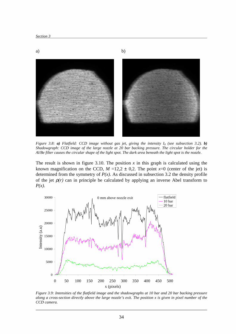
Section 3
34
a) b)
Figure 3.8: a) Flatfield: CCD image without gas jet, giving the intensity I0 (see subsection 3.2). b) Shadowgraph: CCD image of the large nozzle at 20 bar backing pressure. The circular holder for the Al/Be filter causes the circular shape of the light spot. The dark area beneath the light spot is the nozzle. The result is shown in figure 3.10. The position x in this graph is calculated using the known magnification on the CCD, M =12,2 ± 0,2. The point x=0 (center of the jet) is determined from the symmetry of P(x). As discussed in subsection 3.2 the density profile of the jet ρ(r) can in principle be calculated by applying an inverse Abel transform to P(x).
0 mm above nozzle exit
0
5000
10000
15000
20000
25000
30000
0 50 100 150 200 250 300 350 400 450 500x (pixels)
Inte
nsit
y (a
.u)
flatfield10 bar20 bar
Figure 3.9: Intensities of the flatfield image and the shadowgraphs at 10 bar and 20 bar backing pressure along a cross-section directly above the large nozzle’s exit. The position x is given in pixel number of the CCD camera.

Backlighting
35
0 mm above nozzle exit
-1.5
-1.0
-0.5
0.0
0.5
1.0
1.5
2.0
2.5
3.0
-0.5 -0.4 -0.3 -0.2 -0.1 0 0.1 0.2 0.3 0.4 0.5
x (mm)
P (x
)
10 bar10 bar theory20 bar20 bar theory
Figure 3.10: P(x) -as defined in equation (3.10)- directly above the large nozzle’s exit for 10 bar and 20 bar backing pressure, calculated from the data displayed in figure 3.9. The position x is given in mm and is obtained from determining the center of the jet and using the known magnification on the CCD. Also the ‘ theoretical expected’ P(x) is indicated. This is the value obtained from equation (3.10) when taking ρ(r)= ρexit, given by equation (3.5b). The theoretical density profile is thus flat. Note that at the edges only noise is seen, because the flatfield and shadowgraphs images do not cover the complete CCD horizontally, see figure 3.8. Instead the measured P(x) is compared to the P(x) expected from the Laval nozzle theory discussed in subsection 3.1. This theoretical P(x), also shown in figure 3.10, is calculated from eq. (3.10) by taking ρ(r) = ρexit, given by equation (3.5b) (note that the theoretical density profile is therefore flat). It can be seen that the measured and theoretical P(x) correspond reasonably well . At 20 bar backing pressure the value of P(x) is above the theoretical value, whereas P(x) is below the theoretical value at 10 bar. The ‘shape’ of P(x) however is in good agreement with theory, especially for 20 bar. This indicates that the density profile is indeed flat. Remarkable however is that for 10 bar the measured P(x) shows a relatively large deviation from theory around x = 0,3 mm; this also affects the symmetry of the measured P(x). The (general) deviation in figure 3.10 could be due to a different density in the experiment compared to theory. The measured and theoretical values of P(x) then differ by a constant factor. This is investigated in figure 3.11, where the measured P(x) is divided by the theoretical P(x). For 20 bar backing pressure indeed a constant factor of ~1,17 can be found, indicated by the dashed line. For 10 bar the factor is ~0,79 (although for x > 0,1 mm a large deviation can be seen). The gas mass density then is 1,2 kgm-3 and 3,5 kgm-3 at 10 bar resp. 20 bar backing pressure instead of 1,5 kgm-3 resp. 3,0 kgm-3 calculated with eq. (3.5b). The fact that the density at 10 bar backing pressure is lower than the theoretical value, whereas at 20 bar it is higher is not completely understood. A deviation in the nozzle’s dimensions would give the same relative deviation of the density at each backing pressure. Furthermore the uncertainty in the measured backing pressure (about 1 bar) is too little to explain the measured deviations from theory.

Section 3
36
0.0
0.4
0.8
1.2
1.6
2.0
-0.5 -0.4 -0.3 -0.2 -0.1 0 0.1 0.2 0.3 0.4 0.5x (mm)
P(x)
mea
s/P(x
) theo
ry
10 bar20 bar
Figure 3.11: Measured P(x) divided by theoretical P(x) (both given in figure 3.10) for 10 and 20 bar backing pressure. It is more likely that the intensity of the keV radiation from the plasma fluctuates. If the intensity from the plasma in case of the flatfield differs by a factor C from the plasma intensity in case of the shadowgraph, then the measured value of I0(x)/I(x) will be ‘ incorrect’ by a factor C. The value of P(x)= ln(I0(x)/I(x)) then has an offset of ln(C). Note that this factor C may depend on position x (and height z above the nozzle). According to figure 3.10 the offset ln(C) in P(x) is about -0,2 and 0,3 for 10 bar and 20 bar respectively, giving a factor C = 0,8 resp. C = 1,3, which is plausible. Figure 3.12 shows P(x) at 0,5 mm above the nozzle’s exit; this is the position in the gas jet at which a laser beam is usually focused when generating xenon laser plasma.
0,5 mm above nozzle exit
-1.5
-1.0
-0.5
0.0
0.5
1.0
1.5
2.0
2.5
-0.5 -0.4 -0.3 -0.2 -0.1 0.0 0.1 0.2 0.3 0.4 0.5x (mm)
P(x)
10 bar10 bar theory20 bar20 bar theory
Figure 3.12: P(x) 0,5 mm above the large nozzle’s exit for 10 bar and 20 bar backing pressure.

Backlighting
37
As in figure 3.10, also the theoretical value (at the nozzle’s exit) is shown. It can be seen that, especially for 20 bar backing pressure, the measured P(x) is in good agreement with the theoretical P(x) at the nozzle’s exit. This indicates that the gas jet remains well ‘confined’ up to this distance from the exit. The density and diameter of the jet is thus is about the same as at the nozzle exit. However a slightly lower P(x) is found than directly above the nozzle’s exit, cf. figure 3.10, which could be due to fluctuations in the plasma intensity as discussed above. 3.4.2 Small nozzle Shadowgraphs of the gas jet using the small nozzle are recorded for 10, 15, 20, 25 and 30 bar backing pressure. The shadowgraphs at 15 bar and 30 bar are shown in figure 3.14. The nozzle’s exit diameter of 0,41 mm is indicated. From the shadowgraphs P(x) directly above the nozzle’s exit is determined, the result is shown in figure 3.15. The figure also displays the theoretical expected P(x), calculated with eq. (3.10) using a constant ρ(r) = ρexit, given by eq. (3.5a). Well outside the jet, where no absorption is present, P(x) should be 0. The graphs in figure 3.15 are therefore (tentatively) corrected for an offset ln(C), as discussed above in subsection 3.4.1. It can be seen the measured P(x) differs from the theoretical P(x) for all backing pressures, especially at the edges. The shape of the measured P(x) is similar for all backing pressures, and does in any case not correspond with a flat density profile. The radius of the jet appears to be larger than the nozzle’s exit diameter. The above indicates that the jet radially expands. Because especially at the edge of the jet the density will therefore be lower than the theoretical ρexit (for |x| smaller than the radius of the nozzle exit), the deviation between the measured and theoretical P(x) is there the largest. For x close to 0, P(x) will also be lower than theoretically expected due to the lower density at the edges. However, since the density at the center of the jet, which remains higher than at the edges of the jet, is relatively more important for the total absorption (thus P(x)) in case of |x| close to 0, the deviation is less. a) b)
0,41 mm 0,41 mm0,41 mm 0,41 mm Figure 3.14: Shadowgraphs of the small nozzle at 15 bar (a) and 30 bar (b) backing pressure. The nozzle’s exit diameter of 410 µm is indicated.

Section 3
38
a) b) c) d) e)
Figure 3.15: Measured P(x) and theoretically expected P(x) at the small nozzle’s exit for 10, 15, 20, 25 and 30 bar backing pressure. This can be seen in figure 3.15. Note that in the discussion above radial expansion of the jet results in a decreased density but also in an increased path length of absorption.
0 mm above nozzle
0.0
0.1
0.2
0.3
0.4
0.5
0.6
0.7
0.8
0.9
-0.3 -0.2 -0.1 0 0.1 0.2 0.3x (mm)
P(x)
15 bar15 bar theory
0 mm above nozzle
-0.2
0.0
0.2
0.4
0.6
0.8
1.0
1.2
-0.4 -0.3 -0.2 -0.1 0 0.1 0.2 0.3 0.4
x (mm)
P(x)
20 bar20 bar theory
0 mm above nozzle
-0.3
-0.2
-0.1
0.0
0.1
0.2
0.3
0.4
0.5
0.6
-0.3 -0.2 -0.1 0 0.1 0.2 0.3
x (mm)
P(x)
10 bar10 bar theory
0 mm above nozzle
0.0
0.4
0.8
1.2
1.6
2.0
-0.4 -0.2 0 0.2 0.4x (mm)
P(x)
30 bar30 bar theory
0 mm above nozzle
0.0
0.2
0.4
0.6
0.8
1.0
1.2
1.4
1.6
-0.3 -0.2 -0.1 0 0.1 0.2 0.3x (mm)
P(x)
25 bar25 bar theory

Backlighting
39
However, because density decreases as R2 (2-dimensional) and the path length only increases as R, the total absorption measured along a line through the jet at x, thus P(x) will i ndeed decrease.

Section 4: EUV diagnostics
40
4. EUV diagnostics This section gives an overview of the EUV diagnostics used in the experiments of sections 5 and 6. Subsection 4.1 treats the EUV narrowband diagnostic. The broadband EUV pinhole camera is described in the subsection 4.2. Subsection 4.3 discusses the transmission grating spectrograph used in the experiments of section 5. The reflection grating spectrograph used in the prepulse experiments, cf. section 6, will not be discussed. 4.1 EUV narrowband diagnostic In order to monitor the EUV yield emitted in a small wavelength band (which is of interest for lithography application), a narrowband diagnostic consisting of a curved multil ayer mirror and a filtered junction photodiode is used [47,48], see figure 4.1. Radiation emitted from the plasma is collected on the multil ayer mirror. The curvature of the mirror allows the reflected light to be focused on a photodiode. Since the MLM acts as a monochromator (see section 1.2, figure 1.4b in particular), only a small band around a certain EUV wavelength is collected on the diode. However the diode has to be shielded from out of band radiation, e.g. visible light, which is also reflected by the MLM. A filter of 50 nm thick Si3N4 and 100 nm thick Nb is used for this purpose. The transmission of this filter in two different wavelength intervals is shown in figure 4.2. Furthermore the diode is placed in a sealed house to block direct or scattered radiation from the plasma. The radiation power collected on the diode produces a current. The diode is connected to an oscill oscope with an impedance Rscope = 50 Ω, so that a diode signal (in volts) is obtained. The time integrated diode signal (over one EUV pulse) on the scope Sdiode is then given by:
colldiodescopecoll
pulse
diodescopediode EkRdtPkRVsS ⋅== ∫][ (4.1)
with kdiode [A/W] the amount of current produced per watt collected radiation (note that this equals the number of electrons ‘produced’ per eV photon energy). Pcoll is the radiation power collected by the diode, and Ecoll the total collected radiation energy of one EUV pulse. If the radiation energy emitted from the plasma in the bandwidth of the MLM and in 2π sr solid angle is EEUV, the collected energy Ecoll on the diode equals:
plasma
photodiode fil tercurved multil ayer mirror
diode house
plasma
photodiode fil tercurved multil ayer mirror
diode house
Figure 4.1: Narrowband EUV diagnostic consisting of a curved multil ayer mirror and a filtered junction photodiode placed in a house to block direct and scattered radiation from the plasma.
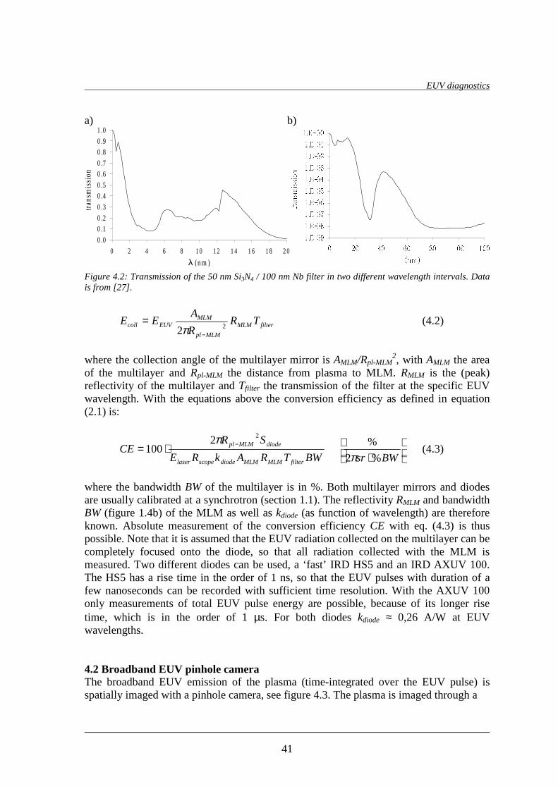
EUV diagnostics
41
a) b)
0.0
0.1
0.2
0.3
0.4
0.5
0.6
0.7
0.8
0.9
1.0
0 2 4 6 8 10 12 14 16 18 20
λ (nm )
tran
smis
sion
Figure 4.2: Transmission of the 50 nm Si3N4 / 100 nm Nb filter in two different wavelength intervals. Data is from [27] .
filterMLM
MLMpl
MLMEUVcoll TR
R
AEE
22 −
=π
(4.2)
where the collection angle of the multil ayer mirror is AMLM/Rpl-MLM
2, with AMLM the area of the multil ayer and Rpl-MLM the distance from plasma to MLM. RMLM is the (peak) reflectivity of the multil ayer and Tfilter the transmission of the filter at the specific EUV wavelength. With the equations above the conversion eff iciency as defined in equation (2.1) is:
BWTRAkRE
SRCE
filterMLMMLMdiodescopelaser
diodeMLMpl22
100 −⋅=π
⋅ BWsr %2
%
π (4.3)
where the bandwidth BW of the multil ayer is in %. Both multil ayer mirrors and diodes are usually calibrated at a synchrotron (section 1.1). The reflectivity RMLM and bandwidth BW (figure 1.4b) of the MLM as well as kdiode (as function of wavelength) are therefore known. Absolute measurement of the conversion eff iciency CE with eq. (4.3) is thus possible. Note that it is assumed that the EUV radiation collected on the multil ayer can be completely focused onto the diode, so that all radiation collected with the MLM is measured. Two different diodes can be used, a ‘ fast’ IRD HS5 and an IRD AXUV 100. The HS5 has a rise time in the order of 1 ns, so that the EUV pulses with duration of a few nanoseconds can be recorded with suff icient time resolution. With the AXUV 100 only measurements of total EUV pulse energy are possible, because of its longer rise time, which is in the order of 1 µs. For both diodes kdiode ≈ 0,26 A/W at EUV wavelengths. 4.2 Broadband EUV pinhole camera The broadband EUV emission of the plasma (time-integrated over the EUV pulse) is spatially imaged with a pinhole camera, see figure 4.3. The plasma is imaged through a
!"#$%&'()*+,-./*+,-.*012344
4 54 64 74 84 044 054 9:;<
=>?@ABCAACD@

Section 4
42
plasma
filterCCD camera
pinhole
plasma
filterCCD camera
pinhole
Figure 4.3: Schematic view of the broadband EUV pinhole camera. small circular pinhole on a CCD camera (Reflex s.r.o., 512 x 512 pixels, 24µm x 24µm pixel size). In order to image only the emission of the plasma in the (broadband) EUV wavelength region, a fil ter is placed between the plasma and the pinhole. A 50 nm Si3N4 / 100 nm Nb filter, see figure 4.2, or a 211 nm thick zirconium (Zr) filter can be used. The transmission of the Zr filter in two different wavelength intervals is given in figure 4.4. The magnification Mpin of the broadband EUV plasma image is:
pinpl
CCDpinpin d
dM
−
−= (4.4)
where dpin-CCD and dpl-pin is the distance from pinhole to CCD and from plasma to pinhole respectively. For the pinhole camera used Mpin = 10,0 ± 0,5. The resolution Rpin of the image on the CCD due to the diameter of the pinhole is: pinpinholepin MdR = (4.5)
whereas the diff raction-limited resolution of the image on the CCD is:
pinhole
CCDpindiff d
dR −⋅
≈λ
(4.6)
a) b)
0
0.1
0.2
0.3
0.4
0.5
0.6
0.7
0.8
0.9
1
0 2 4 6 8 10 12 14 16 18 20λ (nm )
tran
smis
sion
Figure 4.4: Transmission of the 211 nm zirconium filter for two different wavelength intervals. Data is from [27] .
1.E-14
1.E-12
1.E-10
1.E-08
1.E-06
1.E-04
1.E-02
1.E+00
0 20 40 60 80 100 120λ (nm)
tran
smis
sion

EUV diagnostics
43
with dpinhole the diameter of the pinhole. Equations (4.4) to (4.6) give an optimal pinhole diameter, where Rpin = Rdiff:
pinploptpinhole dd −⋅≈ λ, (4.7)
With dpl-pin ≈ 10 cm and λ ≈17 nm at maximum, the optimal diameter of the pinhole is dpinhole,opt ≈ 40 µm. In this study a pinhole with diameter of 50 µm is used. The resolution is thus limited by Rpin. The resolving power of the pinhole image equals (dplasmaMpin)/Rpin
= dplasma/dpinhole, with dplasma the diameter of the plasma. With the diameter of the plasma being ~250 µm at most (see results in sections 5 and 6) the resolving power is ~5 at maximum. Note that Rpin ≈ 500 µm is much larger than the 24 µm pixel size of the CCD, resolution is thus not limited by the CCD. The total broadband EUV emission from the plasma can be obtained by integrating the intensity of the CCD image. Since the response of the CCD is linear with intensity, the emission from different plasmas can be compared quantitatively. 4.3 Transmission grating spectrograph To record the spectrally resolved (time integrated) emission from the plasma in a broad EUV region a spectrograph consisting of a transmission grating and a CCD (Reflex s.r.o) is used, see figure 4.5. The radiation from the plasma is diffracted by the grating, and the normalized intensity I(θ) on the CCD, with θ the angle as defined in the figure, is given by [29, p.404]:
22
sin
sin
sin)(
=
ββ
ααθ
N
NI
θλπα sina= , θ
λπβ sinb= (4.8)
plasma
transmission grating
CCD camera
Zr filter
a=100 nm
b=50 nm
θ
l1 l2
plasma
transmission grating
CCD camera
Zr filter
a=100 nm
b=50 nm
a=100 nm
b=50 nm
θ
l1 l2 Figure 4.5: Schematic view of the transmission grating spectrograph. Emission from the plasma in a broad EUV wavelength region is spectrally resolved on a CCD camera by the diffraction of a transmission grating. A zirconium filter is used to block longer wavelengths to prevent a large intensity in the 0th order, and to suppress out of band radiation. The grating used in this study has N=700 slits, its period a is 100 nm, and the slit width b is 50 nm.

Section 4
44
with N the number of slits of the grating, a the spacing between the slits (grating period) and b the width of the slits (see also figure 4.5), λ is the wavelength of the radiation. An example of the intensity distribution as in equation (4.8) is given in figure 4.6c for a grating with N=5 and b=0,3a. It has the form of a rapidly varying function (sinNα/Nsinα)2, cf. figure 4.6a, representing the interference between different slits, modulated by the function (sinβ/β)2, cf. figure 4.6b, which represents the diffraction of a single slit . The maxima of the rapidly varying function occur when α = mπ, or: λθ ma =sin (4.9) with m = 0, ±1, ±2,…Minima occur when Nα = nπ, or:
λθN
na =sin (4.10)
with n = ±1, ±2… and n/N is not an integer, because then a maximum is present according to eq. (4.9). Equation (4.10) explains the N-1 minima between two maxima in figure 4.6a. The modulating function has minima for β = pπ, or: λθ pb =sin (4.11) with p = ±1, ±2,…The maxima in intensity given by eq. (4.9) are dependent on wavelength, thus emission from the plasma can be spectrally resolved on the CCD. For all wavelengths there is a maximum in intensity in the 0th order (m = 0, sinθ = 0). Therefore, to protect the CCD against high intensity, a zirconium filter is used to block longer wavelengths. For the grating used in this study N = 700, a = 100 nm and b = 50 nm. The fact that in this case a = 2b yields that even maxima (m = ±2, ±4,..) vanish because also the condition for a minimum (p = ±1, ±2,..) is fulfill ed. This is ill ustrated in figure 4.7 where the two intensity functions as in figures 4.6a and 4.6b are shown for this grating. In practice the spectrograph is aligned such that 1st order maxima of a spectrum between roughly 5 and 20 nm are recorded. ‘Disturbance’ by higher order maxima (3rd, 5th, etc.) of shorter wavelengths is neglected because of their low intensity due to the
I
λa
2λa
sinθ0
1
λb
2λb
sinθ sinθ
I
0
1
I
λb
λa
a) b)
0
1
0
1
c)1
0
I
λa
2λa
sinθ0
1
λb
2λb
sinθ sinθ
I
0
1
I
λb
λa
a) b)
0
1
0
1
c)1
0
Figure 4.6: Intensity distribution for a wavelength λ from a transmission grating with N=5 slits and b=0,3a. a) Rapidly varying intensity representing the interference of N slits. b) Modulation function representing the diffraction by a single slit . c) Product of (a) and (b): total intensity distribution of the grating according to equation (4.8), also the modulation ‘envelope’ of (b) is shown.

EUV diagnostics
45
0
1
λa
I
2λa
λb=
sinθ0
1
0
1
λa
I
2λa
λb=
sinθ0
1
Figure 4.7: Intensity distributions for a wavelength λ as in figure 4.6a and b for the grating used in this study with N=700, a=100nm and b=50 nm. Since a=2b even order maxima vanish. modulation part of equation (4.8) (see also figure 4.7). The spectral resolution ∆λgr=λ2-λ1 achievable with the grating is deduced from the fact that the two wavelengths λ1 and λ2, with λ2>λ1, are resolved when the maximum of λ2 (given by eq. (4.9)) coincides with the first minimum of λ1 after a maximum (given by (4.10)). Thus mλ2 = (n/N)λ1, with m =(n-1)/N. The result for the resolving power is:
mNgr
=∆λ
λ (4.12)
with λ=λ1≈λ2. With N = 700 and first order diff raction, m =1, the resolving power is thus 700. For wavelengths in the 7-17 nm range (FWHM of the Zr filter) this yields a resolution of ∆λgr = 0.10-0.24 Å. However resolution is also determined by geometrical aspects of the spectrograph. The finite size of the plasma and the grating namely result in a spreading of the plasma emission imaged on the CCD. The distance ∆x over which radiation from the plasma is spread on the CCD is:
gratingplasmagrating dddl
lx ++=∆ )(
1
2 (4.13)
with l1 and l2 the distance from plasma to grating and from grating to CCD respectively, cf. figure 4.5. dgrating is the total width of the grating, dplasma the diameter of the plasma. The condition for a maximum in intensity eq. (4.9) can be written as mλ=a(x/l2) for small angles, sinθ ≈θ ≈x/l2, where x is the distance on the CCD from axis to the mth order maximum. The geometrical resolution is then given by:
+
+=∆=∆
212 l
aN
l
aNd
m
ax
ml
a plasmageoλ (4.14)
using eq. (4.13) and dgrating = aN. In the set-up l1 = 0,61 m and l2 = 0,090 m. This gives a resolution of 1,3 Å, when taking dplasma = 250 µm (result from pinhole pictures, see section 5) and m=1. Note that from equation (4.14) the CCD resolution is ∆λCCD=(a/m· l2)∆x, where ∆x=24 µm is the CCD pixel size in this case, giving ∆λCCD =

Section 4
46
0,26Å. The resolution of the spectrograph is thus limited by geometrical aspects (size of the plasma and grating) and equals ~1,3 Å. Calibration of the wavelength scale of the spectrum on the CCD is done by identification of four intense O5+ lines from plasma generated on CO2 target gas. The wavelength and transition corresponding with these lines are given in table 4.1. A spectrum of ‘CO2 plasma’ is shown in figure 4.8, the lines used for calibration are indicated. To obtain the real (relative) intensity at each wavelength, the spectrum recorded on the CCD has to be corrected for the Zr filter transmission, cf. figure 4.4, and for the grating eff iciency. This grating eff iciency reflects the wavelength dependence of the transmission of the grating, and is given in figure 4.9 using [31] for the grating of the spectrograph used in this study. Table 4.1: Transitions in O5+ and corresponding wavelengths of the lines used for the calibration of the wavelength scale of the spectrograph. Data is from [30] .
Transition Configuration J - J
Wavelength (Å)
1s22s - 1s24p 1/2 - ³/2 115.822 1s22p - 1s24d 1/2 - ³/2 129.785 1s22s - 1s23p 1/2 - ³/2 150.089 1s22p - 1s23d ³/2 -
5/2 173.082
Figure 4.8: Spectrum of plasma generated on CO2 target gas. The lines used for wavelength calibration are indicated.
Figure 4.9: Grating efficiency for the grating of the spectrograph used in this study, calculated using [31] . The grating consists of 300 nm thick Si3N4 coated with 5 nm Au.
wavelength (Å)
grat
ing
eff
icie
ncy
0 100 200 300 4000.00
0.05
0.10
0.15
0.20300 nm Si3N4 + 5 nm Au
wavelength (Å)
grat
ing
eff
icie
ncy
0 100 200 300 4000.00
0.05
0.10
0.15
0.20300 nm Si3N4 + 5 nm Au
0
100
200
300
400
500
600
700
800
70 80 90 100 110 120 130 140 150 160 170 180 190 200
λ (Å)
Inte
nsit
y (a
.u.)
0
100
200
300
400
500
600
700
800
70 80 90 100 110 120 130 140 150 160 170 180 190 200
λ (Å)
Inte
nsit
y (a
.u.)
0
100
200
300
400
500
600
700
800
70 80 90 100 110 120 130 140 150 160 170 180 190 200
λ (Å)
Inte
nsit
y (a
.u.)

Section 5: Laser plasma parameter study
47
5. Laser plasma parameter study EUV emission from laser plasma generated on a supersonic xenon jet has been investigated for different laser intensities and initial target gas densities. Subsection 5.1 presents spectrally resolved emission from xenon plasma generated with a KrF excimer laser for these different laser- and target conditions. The KrF laser intensities are in the order of 1012 Wcm-2. The results led to the development of a simple theoretical model for the dependence of spectral intensity on initial target gas density. This model will be discussed in subsection 5.2. Results of narrowband EUV yield as function of target gas density are presented and compared to the model in subsection 5.3, also the KrF excimer laser is used in these measurements. Subsection 5.4 presents spectra of xenon plasma generated at higher laser intensities, in the order 1013 Wcm-2, using a Nd:YAG laser. Also in these measurements the dependence of spectral intensity on initial target gas density has been investigated, and is compared with the results from the KrF laser plasmas, and the theoretical model. Spectral li nes of Xe6+ to Xe10+ in the EUV wavelength region, which are classified in literature [32,33,34], see Appendix, are used in the analysis of xenon spectra. The set-up used for the laser plasma parameter study is shown in figure 5.1. The laser beam is coupled into the vacuum chamber through a window, and is focused on the gas jet by a lens. The focal spot of the laser is positioned 0,5 mm above the nozzle exit. The used diagnostics, which are described in section 4, are indicated.
+
vacuum chamber
laser beam
lens
nozzle
Broadband EUV pinhole camera
MLM
diode
Transmission grating spectrograph
+
vacuum chamber
laser beam
lens
nozzle
Broadband EUV pinhole camera
MLM
diode
Transmission grating spectrograph
Figure 5.1: Experimental set-up used for the laser plasma parameter study. The EUV diagnostics, described in section 4, are indicated. The pinhole camera and spectrograph are both differentially pumped. 5.1 Spectrally resolved emission using a KrF excimer laser Xenon plasma is generated with a KrF excimer laser (lambda physik LPX 350). The large nozzle (cf. section 3) is used. Spectra are recorded at four different laser pulse energies at 10 bar and 20 bar backing pressure. The used laser pulse energies are 480 ± 10 mJ, 670 ± 10 mJ, 780 ± 10 mJ and 850 ± 10 mJ. With the excimer laser pulse length being 27 ns (FWHM) and the focal spot diameter being ~50 µm these energies correspond to laser intensities of ~0,9⋅1012 W/cm2, ~1,3⋅1012 W/cm2, ~1,5⋅1012 W/cm2 and ~1,6⋅1012 W/cm2 respectively. However, with this laser, decreasing the pulse energy can increase the

Section 5
48
divergence of the beam and thus increase the focal spot size. The given intensities are therefore a global indication. 5.1.1 Xenon spectrum Figure 5.2 shows xenon spectra for 480 mJ and 850 mJ laser pulse energy at 10 bar backing pressure. A (tentative) classification of the spectrum at 850 mJ is indicated in the figure and will be discussed below. The lines at 170,1 Å, 173,3 Å, 175,8 Å, 177,3 Å, and 179,9 Å can be attributed to Xe7+. Lines of Xe7+ at 123,3 Å and 166,7 Å given in literature can not be seen in the spectrum. Most probably these lines can not be resolved from other neighboring lines. The lines at 85,4 Å, 88,5 Å, 96,2 Å, 100,9 Å, 103,5 Å, 119,5 Å, 161,3 Å and 165,4 Å can be attributed to Xe8+. The lines at 110,2 Å, 112,3 Å and 116,4 Å, and line emission between 140 Å and 160 Å can be attributed to Xe9+. Remarkable is that at 150 Å, where Xe9+ should have high emission, the intensity is low. Absorption at this wavelength by Xe9+ could give an explanation, but is however not yet understood. The absorption at 150 Å could also be from O5+, due to contamination of the target gas with oxygen or CO2. Absorption from O5+ at other wavelengths (see table 4.1) can not be seen, however the (emission) line at 173,3 Å could also be from O5+. Emission between 108 Å and 112 Å and the intense line at 124,6 Å could be from Xe10+, however if Xe10+ population would be considerable also high intensity between 130 Å and 140 Å (especially at 135 Å) should be seen, which is not the case. The three lines from Xe6+ given in the Appendix are diff icult to distinguish from Xe7+ lines, except the line at 185,4 Å. Emission at this wavelength is low in the spectrum of f igure 5.2. The lines of relatively high intensity at 92,1 Å, 128,3 Å and 164,4 Å, indicated by a question mark, could not be attributed to any of the ionization stages in the Appendix. The weak lines between 130 Å and 140 Å are tentatively attributed to Xe10+, however the lines at 133,4 Å, 134,5 Å, 137,0 Å and 138,6 Å could in principle also be from Xe9+.
0
500
1000
1500
2000
2500
3000
3500
4000
70 80 90 100 110 120 130 140 150 160 170 180 190 200
λ (Å)
Inte
nsit
y (a
.u)
850 mJ480 mJ
Xe8+
Xe7+
?
Xe8+
Xe8+
Xe9+
?
Xe10+(?)
?Xe9+
Xe10+
Xe6+(?)
Figure 5.2: Xenon spectrum for 480 mJ and 850 mJ excimer laser pulse energy at 10 bar backing pressure. A classification is given using the data in the Appendix.

Laser plasma parameter study
49
In conclusion, it can be stated that the main ionization stages present are Xe7+, Xe8+ and Xe9+. 5.1.2 Dependence of spectral intensity on laser pulse energy The dependence of spectral intensity on laser pulse energy at 10 bar backing pressure is shown in figure 5.3a. The spectral intensities at 670 mJ, 780 mJ and 850 mJ pulse energy are divided by the spectral intensity at 480 mJ pulse energy. Figure 5.3b shows the dependence of the conversion efficiency on laser pulse energy. The conversion eff iciencies at 670 mJ, 780 mJ and 850 mJ pulse energy are divided by the conversion eff iciency at 480 mJ pulse energy. In this case the conversion eff iciency is obtained by dividing the spectral intensity by the corresponding laser pulse energy. Note that each graph in figure 5.3b thus only differs by a constant factor (independent of wavelength) from the corresponding graph in figure 5.3a. From figure 5.3a, an increase in intensity over the whole spectrum can be seen for each graph. The increase of spectral intensity with laser pulse energy is the highest between 110 Å and 120 Å and between 140 Å and 160 Å. Also a relatively large increase in intensity at 85,4 Å can be seen. The two mentioned wavelengths regions, where increase is highest, correspond to Xe9+, the line at 85,4 Å corresponds to Xe8+. From figure 5.3b, the increase in conversion eff iciency in the wavelength regions 110 Å - 120 Å and 140 Å - 160 Å, is at maximum about a factor 1,9 respectively 2, comparing the highest pulse energy, 850 mJ, with the lowest pulse energy, 480 mJ. The conversion eff iciency at the 85,4 Å line increases by a factor 2,2 at maximum. In the wavelength region 120 Å – 140 Å conversion also eff iciency increases with laser pulse energy, maximum increase at 135 Å is about a factor 1,3. The conversion eff iciency of the Xe7+ lines above 170 Å does not increase much with pulse energy; the CE ratio in figure 5.3b is close to 1. As the temperature of the plasma is increased by increasing the laser intensity, higher ionization stages become relatively more populated, whereas lower ionization stages become relatively less populated, see section 2.6.3. a) b) Figure 5.3: Dependence of spectral intensity on excimer laser pulse energy at 10 bar backing pressure. a) The intensities at 670 mJ, 780 mJ and 850 mJ pulse energy divided by the intensity at 480 mJ pulse energy. This is indicated by the labels. b) Conversion efficiencies at 670 mJ, 780 mJ and 850 mJ laser pulse energy divided by conversion efficiency at480 mJ pulse energy. The (spectrally resolved) conversion efficiency is obtained by dividing the spectral intensity by the corresponding laser pulse energy.
! "# $
%&'%&( )* +,- . /+-
012 3 412567 8 9:7
;<;=>?@AB@ACDEFDEGHIJHIKLMN
OP QR ST UTT UUT UVT UWT UXT UYT Z[\ Z]\ Z^\ _` a
bcbd ef ghi j kgi
lmn o pmnqrs t uvs
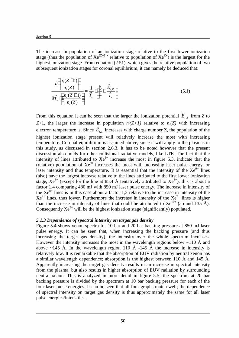
Section 5
50
The increase in population of an ionization stage relative to the first lower ionization stage (thus the population of Xe(Z+1)+ relative to population of XeZ+) is the largest for the highest ionization stage. From equation (2.51), which gives the relative population of two subsequent ionization stages for coronal equili brium, it can namely be deduced that:
+⋅=
+⋅∂
+∂
e
Zi
e
i
ie
i
i
T
E
T
Zn
ZnT
Zn
Zn
ˆ
ˆ
4
3ˆ1
)(
)1(ˆ
)(
)1(
, (5.1)
From this equation it can be seen that the larger the ionization potential ZiE ,ˆ from Z to
Z+1, the larger the increase in population ni(Z+1) relative to ni(Z) with increasing
electron temperature is. Since ZiE ,ˆ increases with charge number Z, the population of the
highest ionization stage present wil l relatively increase the most with increasing temperature. Coronal equili brium is assumed above, since it will apply to the plasmas in this study, as discussed in section 2.6.3. It has to be noted however that the present discussion also holds for other colli sional radiative models, li ke LTE. The fact that the intensity of lines attributed to Xe9+ increase the most in figure 5.3, indicate that the (relative) population of Xe9+ increases the most with increasing laser pulse energy, or laser intensity and thus temperature. It is essential that the intensity of the Xe9+ lines (also) have the largest increase relative to the lines attributed to the first lower ionization stage, Xe8+ (except for the line at 85,4 Å tentatively attributed to Xe8+), this is about a factor 1,4 comparing 480 mJ with 850 mJ laser pulse energy. The increase in intensity of the Xe8+ lines is in this case about a factor 1,2 relative to the increase in intensity of the Xe7+ lines, thus lower. Furthermore the increase in intensity of the Xe9+ lines is higher than the increase in intensity of lines that could be attributed to Xe10+ (around 135 Å). Consequently Xe9+ will be the highest ionization stage (significantly) populated. 5.1.3 Dependence of spectral intensity on target gas density Figure 5.4 shows xenon spectra for 10 bar and 20 bar backing pressure at 850 mJ laser pulse energy. It can be seen that, when increasing the backing pressure (and thus increasing the target gas density), the intensity over the whole spectrum increases. However the intensity increases the most in the wavelength regions below ~110 Å and above ~145 Å. In the wavelength region 110 Å -145 Å the increase in intensity is relatively low. It is remarkable that the absorption of EUV radiation by neutral xenon has a similar wavelength dependence; absorption is the highest between 110 Å and 145 Å. Apparently increasing the target gas density results in an increase in spectral intensity from the plasma, but also results in higher absorption of EUV radiation by surrounding neutral xenon. This is analyzed in more detail i n figure 5.5; the spectrum at 20 bar backing pressure is divided by the spectrum at 10 bar backing pressure for each of the four laser pulse energies. It can be seen that all four graphs match well; the dependence of spectral intensity on target gas density is thus approximately the same for all l aser pulse energies/intensities.

Laser plasma parameter study
51
0
2000
4000
6000
8000
10000
12000
70 80 90 100 110 120 130 140 150 160 170 180
λ (Å)
Inte
nsit
y (a
.u.)
10 bar20 bar
Figure 5.4: Xenon spectra at 10 and 20 bar backing pressure. Excimer laser pulse energy is 850 mJ.
0.0
1.0
2.0
3.0
4.0
5.0
6.0
70 80 90 100 110 120 130 140 150 160 170 180λ (Å)
I m,2
0/I m
,10
(-)
850 mJ780 mJ670 mJ480 mJfitcurve
Figure 5.5: Dependence of spectral intensity on target gas density. For each excimer laser pulse energy the spectrum at 20 bar backing pressure is divided by the spectrum at 10 bar backing pressure. A curve fit given by equation (5.2) is applied to the data. A curve of the form:
( )fitfitm
m xKI
I)()(exp
)(
)(
10,
20, ∆⋅−⋅= ρλκλλ
(5.2)
is fitted to the data for 850 mJ pulse energy in figure 5.5. Im(λ) is the measured spectral

Section 5
52
intensity, subscripts 10 and 20 denote 10 respectively 20 bar backing pressure. The fit thus implies that the spectral intensity increase by a constant factor Kfit (independent of wavelength). The exponential term in (5.2) describes the (increased) EUV absorption by neutral xenon, with κ(λ) the specific absorption coeff icient of xenon (as defined in equation (3.7)), and (ρ∆x)fit a certain xenon mass density times path length. The specific absorption κ(λ) coeff icient of xenon in the wavelength range 70 Å – 180 Å is given in figure 5.6, data from [27] is used. Subsection 5.2 will give a more detailed theoretical model for the applied fit. The result of the least square fit is Kfit=4,64 ± 0,20 and (ρ∆x)fit = (10,6 ± 1,1)· 10-5 kgm-2. The result for (ρ∆x)fit corresponds to a (more commonly used) xenon pressure times path length of p∆x=1,50 ± 0,15 Torr· cm at a temperature of 295 K. Note that the error bars given for the fit parameters Kfit and (ρ∆x)fit indicate the range of possible values at which the least square fit is obtained. The two fit parameters are however coupled, since a certain value for Kfit within its given range implies a fixed value for (ρ∆x)fit. This is shown in figure 5.7, where the isolines indicate the sum of the squared errors between the measured data and the fit of f igure 5.5 as function of Kfit and (p∆x)fit.
0.0
0.2
0.4
0.6
0.8
1.0
1.2
1.4
70 80 90 100 110 120 130 140 150 160 170 180
λ (Å)
κ (1
04 kg-1
m2 )
Figure 5.6: Specific absorption coefficient κ(λ) of neutral xenon in the wavelength range 70 Å – 180 Å. Data from [27] is used.
K fit
(p∆ x
) fit
(Tor
r·cm
)
K fit
(p∆ x
) fit
(Tor
r·cm
)
Figure 5.7: Sum of squared error between measured data and fit of figure 5.5 as function of the two fit parameters Kfit and (p∆x)fit. The minimum value is 29,6.

Laser plasma parameter study
53
5.2 Model for dependence of spectral intensity on target gas density In analyzing the dependence of the spectral intensity on initial target gas density, as shown in figure 5.5, it apparently has to be taken into account that, when increasing the target gas density, the absorption of EUV radiation from the plasma by surrounding neutral xenon increases as well . The measured spectral intensities Im(λ) at 10 bar respectively 20 bar backing pressure may therefore be written as:
( )1010,10, )()(exp)()( xII plm ∆⋅−⋅= ρλκλλ
( )2020,20, )()(exp)()( xII plm ∆⋅−⋅= ρλκλλ (5.3)
where Ipl(λ) is the spectral intensity directly from the plasma, as if no EUV absorption by neutral xenon is present. The exponential terms represent the absorption of the EUV radiation, with κ(λ) the specific absorption coefficient of xenon, given in figure 5.6, and (ρ∆x) the xenon mass density times the path length of absorption. From equation (5.3) the ratio of the measured spectral intensities becomes:
( )( )102010,
20, )()()(exp)()(
)(xxK
I
I
m
m ∆−∆⋅−⋅= ρρλκλλλ
)(
)()(
10,
20,
λλ
λpl
pl
I
IK = (5.4)
Comparing this with the fit formula, given in equation (5.2), thus implies that (ρ∆x)fit= (ρ∆x)20 - (ρ∆x)10 and Kfit=K(λ). The factor (ρ∆x)fit thus indeed indicates the increased absorption of EUV radiation by the neutral surrounding xenon, when increasing the backing pressure from 10 bar to 20 bar. The obtained result of (ρ∆x)fit = (10,6 ± 1,1)· 10-5 kgm-2, yields that the transmission of EUV at a wavelength of 13,5 nm is a factor 3,5 ± 0,4 lower at 20 bar backing pressure than at 10 bar. The initial neutral xenon density is linear with the backing pressure, see also subsection 3.1, equation (3.5). In that case (ρ∆x)20 =2· (ρ∆x)10, and thus (ρ∆x)20 =2· (ρ∆x)10 = (21,2 ± 2,2)· 10-5 kgm-2. This yields a transmission of 0,29 ± 0,04 and 0,08 ± 0,02 at 10 and 20 bar backing pressure respectively for 13,5 nm EUV radiation. Kfit is the ratio of intensities Ipl(λ) at 20 and 10 bar backing pressure. A model for Kfit (which is independent of wavelength) will be given below. In this model coronal equili brium is applied, the validity of coronal equili brium for the plasmas under study is discussed in section 2.6.3. Furthermore it is assumed that the electron temperature and the dimensions of the plasma are approximately independent of initial target gas density. The latter assumption is confirmed by pinhole measurements. The electron colli sional excitation rate of an atom or ion from level p to q, averaged over a Maxwelli an electron velocity distribution, is given by [35]:

Section 5
54
∆−
∆>∝<
e
pq
epq
eepqe
T
E
TE
nvn
ˆ
ˆexp
ˆˆ 2/1σ [s-1] (5.5)
with σpq the cross-section for colli sional excitation and ve the electron velocity.
pqpq EEE ˆˆˆ −=∆ is the difference in energy between level p and q in eV, and ne and eT
are the electron density and temperature (in eV) respectively. If the plasma is in coronal equili brium, a balance exists between colli sional excitation of a xenon ion from the ground state to an excited state and radiative de-excitation of this excited state to the ground state:
)()0(0
qXeXe Z
h
e
Z
q
++
←→
ν
(5.6)
This implies that the coll isional excitation rate equals the radiative de-excitation rate:
0
00000
q
eqeqqqeqe A
vnnnAnvnn
><=⇒>=<
σσ (5.7)
with n0 the density of the ground state, nq the density of the excited state q, and Aq0 the transition probabili ty for radiative de-excitation given by equation (2.45). Note that since Aqp is proportional to Epq squared, radiative de-excitation of an excited state to the ground state (Epq = E0q is maximum) will be dominant as compared to de-excitation to a lower excited state. Population of excited states by colli sional excitation will be mainly from the ground state, since the density of the ground state is (much) higher than of the excited states (despite the fact that the colli sional excitation rate decreases with higher ∆Epq). This justifies the equili brium balance, equations (5.6) and (5.7). The radiation density Jqp of a spectral li ne corresponding with the transition q→p is given by equation (2.44). Substituting equations (2.45), (5.5) and (5.7) in eq. (2.44) results in:
∆−⋅
∆
∆∝
e
q
oq
pq
e
eqp
T
E
E
E
T
nnJ
ˆ
ˆexp
ˆ
ˆ
ˆ0
3
2/10 (5.8)
If it is assumed now that the electron temperature of the generated plasma is approximately independent of the initial target gas density, the relative population of the different ionization stages will not change with initial target gas density. The relative population of ionization stages is namely only dependent on electron temperature for coronal equili brium, cf. equation (2.51). Hence the electron density ne is proportional to the initial target gas density na0, since the average degree of ionization (Z*) does not change. The increase in ne with increasing na0 will shift the corona balance from the ground state to the excited states, equation (5.7). The density n0 of the ground states of the ions will t herefore increase less then proportional with increasing na0. However, since the density n0 will be (much) higher than the density of the excited states, it can actually be

Laser plasma parameter study
55
stated that n0 is approximately proportional to na0. Pinhole pictures taken of the plasma for the different backing pressures and laser pulse energies show no significant change in the dimensions of the (broadband EUV emitting part of the) plasma. All plasmas measure 120 ± 10 µm FWHM vertically (perpendicular to the laser beam) and 250 ± 20 µm FWHM horizontally (parallel to the laser beam). The volume (and surface) of the generated plasma is about the same for different initial target gas densities. The ratio of two spectral intensities at different backing pressures or laser pulse energies then equals the ratio of the two corresponding radiation densities. The above then finally gives the following result for K(λ):
−∆
==
20,10,
0
2/1
20,
10,
2
10,0
20,0
10,
20,
ˆ1
ˆ1ˆexp
ˆ
ˆ
)(
)()(
ee
q
e
e
a
a
pl
pl
TTE
T
T
n
n
I
IK
λλ
λ (5.9)
where for the electron temperatures at 10 and 20 bar backing pressure 20,10,ˆˆee TT ≈ holds
(such that the relative population of ionization stages remains about the same). An increase in backing pressure from 10 bar to 20 bar will result in a increase in initial xenon target gas density by a factor 2, as discussed above. If electron temperature remains exactly the same, this yields that K(λ)=Ipl,20(λ)/Ipl,10(λ) ≈ 22 = 4, which is already in good agreement with the value Kfit=K(λ) = 4,64 ± 0,20 obtained from the fit in figure 5.5. The additional increase in intensity, such that Kfit > 4, can be explained by a (small )
increase 20,eTd in electron temperature 20,eT with respect to 10,eT . From equation (5.9) it
can namely be deduced that:
2
1ˆˆ
ˆ
)(
)(
20,
0
20,
20, −∆
=∂
∂
e
q
e
e
T
E
T
T
K
K
λλ
(5.10)
For the spectral range considered in figures 5.4 and 5.5 pqE∆ is minimum 69 eV,
corresponding with λpq=180 Å. Since pqq EE ˆˆ0 ∆≥∆ , also qE0
ˆ∆ > 69 eV. Considering the
ionization stages present, the electron temperature will be about 30 eV, see section 2.6.3, figure 2.6 in particular. With K(λ) being 4,64 ‘ instead’ of 4, ∂K(λ)/K(λ) = 0,16.
Substituting the above in eq. (5.10) then yields that 20,20,ˆ/ˆee TT∂ < 0,09, thus increase in
electron temperature is smaller than 9 % (or smaller than 2,7 eV, when taking an electron temperature of 30 eV at 10 bar backing pressure). An increase in electron temperature, although small , will also change the relative population of the ionization stages. The highest ionization stages present become relatively more populated, the lower ionization stages less. This results in an additional increase in electron density, and thus an increase in spectral intensity, cf. eqs. (5.8) and (5.9). The increase in temperature when increasing backing pressure may therefore be even less than discussed above, where equation (5.10) was used. A change in the relative population of the ionization stages due to an increase in temperature may also explain the fact that the increase in spectral intensity in the wavelength regions 105 Å-113 Å and 130 Å-160 Å is relatively large and exceeds the

Section 5
56
fitted value, while the increase in the wavelength region 170 Å -180 Å is less than the fitted value. The first two regions namely contain lines corresponding with ionization stages Xe9+ and Xe10+, which become relatively higher populated. The region 170 Å -180 Å contains lines of Xe7+, which becomes less populated. Note that a relatively large increase in intensity of the line at 85,4 Å (from Xe8+) when increasing the target gas density can be seen in figure 5.5. Increasing the laser pulse energy also resulted in a relatively large increase in intensity of this line, see figure 5.3. As discussed in section 2.6.1 continuum radiation density is proportional to ne
2Z. From the discussion above the intensity of continuum radiation then also is, as line radiation, proportional to na0
2. An increase in spectral intensity higher than a factor (na0,20 /na0,10)2,
when increasing backing pressure from 10 bar to 20 bar, could also be explained by an additional increase in temperature. According to the model discussed above, the temperature of the generated plasma, and therefore the energy per particle (electrons and ions), is approximately independent on initial target gas density. As the initial target gas density increases by e.g. a factor C, the electron and ion density increase by the same factor, and hence the total number of particles in the plasma increases by a factor C (the dimensions of the plasma remains the same). The total energy in the plasma, thus the absorbed laser energy, then also increases by a factor C. From equation (2.32) the absorption coeff icient for inverse Bremsstrahlung αIB is proportional to the electron density squared, ne
2. This yields that αIB increases by a factor C2. The part of the laser light absorbed in the plasma by inverse Bremstrahlung is 1-exp(-αIB∆z) (see also equation (2.27)), with ∆z the length of the plasma over which the absorption takes place. In the case that absorption of laser light is low, αIB∆z << 1, the absorbed laser light also increases by a factor C2. In the (limiti ng) case that all l aser light is absorbed, αIB∆z >>1, the absorbed laser light will be independent on the electron density in the plasma. For example in the measurements presented in section 5.1.3, the initial target gas density increased approximately by a factor C = 2, by increasing backing pressure from 10 to 20 bar. An increase in absorbed laser light also by a factor C = 2, as discussed, would yield that: (1-exp(-4αIB∆z))/(1-exp(-αIB∆z)) = 2, where αIB in this case is the value for the lowest density (at 10 bar backing pressure). The result is αIB∆z = 0,6. This yields that for 10 bar backing pressure 1-exp(-0,6) = 0,45 part of the laser light is absorbed and for 20 bar backing pressure 1-exp(-2,4) = 0,90 part of the laser light is absorbed. 5.3 EUV narrowband yield versus target density using a KrF excimer laser The EUV yield at both 11, 4 nm and 13,0 nm is measured as function of backing pressure with two separate narrowband diagnostics. The small nozzle (cf. section 3) is used in this experiment. The KrF excimer laser (lambda physik LPX 350) is used to generate the laser plasmas. The pulse energy is 890 ± 10 mJ, which corresponds to an intensity of (1,7 ± 0,2)⋅1012 W/cm2. Figure 5.8 shows the conversion eff iciencies CE, as given by equations (2.1) and (4.3), at 11,4 nm and 13,0 nm versus backing pressure. Maximum conversion eff iciency is (3,1 ± 0,2)⋅10-3 % / (2πsr· %BW) and (0,72 ± 0,04)⋅10-3 % / (2πsr· %BW) at 11,4 nm and 13,0 nm respectively. A curvefit is applied to both graphs. It has the form CE ∝ pback
2· exp(-kfit· pback), corresponding with the theoretical model discussed in subsection 5.2, where the initial target gas density na0 is linear with the backing pressure

Laser plasma parameter study
57
pback, and kfit is a constant. Note that kfit is thus ‘analogue’ to (ρ∆x)fit, used above. Both fit parameters involve the absorption by neutral xenon, kfit should thus not be confused with the parameter Kfit used above. Here Kfit actually equals the squared quotient of two backing pressures (e.g. 20 bar divided by 10 bar). Note that an increase in intensity from the plasma additional to the factor na0
2 by an increase in temperature, as discussed in subsection 5.2, equation (5.10) in particular, is thus neglected in the fit applied here. The result of the fit is kfit = 0.084 ± 0.002 for 11,4 nm and kfit = 0.077 ± 0.002 for 13,0 nm. This yields that the xenon mass density times path length of absorption at 10 bar backing pressure is (ρ∆x)10 = (7,4 ± 0,2)· 10-5 kg/m2 and (ρ∆x)10 = (6,2 ± 0,2)· 10-5 kg/m2 at 11,4 nm and 13,0 nm respectively calculated with the result for kfit and the specific absorption coeff icient κ(λ), cf. figure 5.6,. This is close to the result (ρ∆x)10 = (10,6 ± 1,1)· 10-5 kgm-2 found from the curve fitted to the spectrally resolved data in figure 5.5. The deviation can be explained by the fact that the orientation of the spectrograph and the narrowband diagnostics with respect to the gas jet is not the same, this may result in a different path (length) of radiation through the EUV absorbing neutral xenon surrounding the plasma. Moreover a different nozzle is used. The fact that the results for (ρ∆x)10 found with the two narrowband measurements at 11,4 nm and 13,0 nm respectively are not consistent, could be explained in a similar way. The two narrowband diagnostics are namely also not orientated exactly the same with respect to the gas jet. Note that the model discussed in subsection 5.2, predicts a decrease in EUV yield (and thus conversion eff iciency) above a certain backing pressure, where the increase in absorption by the neutral xenon becomes larger than the increase in intensity from the plasma. This can also be seen from the curve fits in figure 5.8, for backing pressures higher than ~25 bar. However no measurements could be done at these high backing pressures to verify this prediction. a) b) Figure 5.8: Conversion efficiency at 11,4 nm (a) and 13,0 nm (b) versus backing pressure. A curve fit, corresponding to the model discussed in subsection 5.2, is applied to both graphs. The excimer laser pulse energy is 890 ± 10 mJ.
0.0
0.5
1.0
1.5
2.0
2.5
3.0
3.5
0 5 10 15 20 25 30backing pressure (bar)
CE
(10-3
% /
(2ps
r%B
W))
0
0.1
0.2
0.3
0.4
0.5
0.6
0.7
0.8
0 5 10 15 20 25 30backing pressure (bar)
CE
(10-3
% /
(2ps
r%B
W))

Section 5
58
5.4 Spectrally resolved emission using a Nd:YAG laser In the experiments discussed in this subsection xenon plasmas are generated using a Nd:YAG laser (Continuum PL 8010) and the large nozzle (cf. section 3). Spectra are recorded at 10 and 20 bar backing pressure at 3 different laser pulse energies. The laser pulse energies are 380 ± 5 mJ, 452 ± 5 mJ and 650 ± 5 mJ. With the laser pulse length being 6 ns (FWHM) and a focal spot diameter of typically ~30 µm, this yields laser intensities of (0,90 ± 0,01)⋅1013 Wcm-2, (1,07 ± 0,01)⋅1013 Wcm-2 and (1,53 ± 0,01)⋅1013 Wcm-2 respectively. These intensities are an order in magnitude higher than the laser intensities obtained with the KrF excimer laser, see subsection 5.1. It is therefore expected that a higher plasma temperature can be reached with the Nd:YAG laser. Note that with this laser the focal spot size will not change with pulse energy. 5.4.1 Xenon spectrum Figure 5.9 shows xenon spectra for all three laser pulse energies at 10 bar backing pressure. A tentative classification of the spectrum at 650 mJ is indicated. The lines at 181,3 Å and 184,9 Å can be attributed to both Xe6+ and Xe7+. The lines at 170,8 Å, 175,5 Å, 178,2 Å and 179,2 Å can be attributed to Xe7+. The line at 173,1 Å could be from Xe7+, but also from O5+, due to CO2 contamination of the xenon target gas (see table 4.1). The line at 129,2 Å also indicates the presence of O5+. Note that O5+ lines at 115,8 Å and 150,1 Å, which also should be seen in this case, probably can not be resolved from other lines. The lines at 85,3 Å, 85,5 Å, 162,1 Å, 165,3 Å and 168,4 Å can be attributed to Xe8+. Lines in the wavelength interval 140 Å to 160 Å can be attributed to Xe9+. The line at 124,1 Å and lines in the wavelength interval 131,5 Å to 140,3 Å can be attributed to Xe10+.
0
5000
10000
15000
20000
25000
70 80 90 100 110 120 130 140 150 160 170 180 190
λ (Å)
Inte
nsity
(a.
u)
650 mJ452 mJ380 mJ
Xe7+
O5+
Xe6+/
Xe7+
Xe8+
Xe8+Xe9+
Xe10+,
Xe10+
Xe9+
Xe10+
>Xe10+
O5+
Figure 5.9: Xenon spectra for 380 mJ, 452 mJ and 850 mJ Nd:YAG laser pulse energies at 10 bar backing pressure. A tentative classification is given using the Appendix.

Laser plasma parameter study
59
The unresolved transition array (UTA) around 110 Å, can contain lines from Xe10+ in the wavelength interval 105,2 Å to 113,0 Å and from Xe9+ in the wavelength interval 110 Å to 116,5 Å. Also higher ionization stages than Xe10+ can contribute to lines around 110 Å [36]. Lines at 92,1 Å and 128,3 Å, which are present in the spectra of f igure 5.2, and which could not be attributed, can also be seen in the spectra in figure 5.9. Note that some of the lines from Xe7+ and Xe8+ that are present in the spectra in figure 5.2 are not seen in the spectrum in figure 5.9. Comparing this xenon spectrum recorded using the Nd:YAG laser with the spectrum recorded using the KrF excimer laser, cf. figure 5.2, it is clear that emission from Xe10+ is (relatively) much higher. This is expected, since higher plasma temperatures can be obtained with the Nd:YAG laser, due to the higher laser intensity. Consequently higher ionization stages become relatively more populated. Remarkable is the high intensity at short wavelengths (from roughly 70 Å to 80 Å), which is probably from ionization stages >Xe10+. 5.4.2 Dependence of spectral intensity on laser pulse energy In figure 5.9 it can be seen that, when increasing the laser pulse energy from 380 mJ to 452 mJ, the spectral intensity increases by roughly the same amount for all wavelengths; the relative intensity of the structures approximately remains the same. Increasing the pulse energy to 650 mJ leads to a relatively high increase in intensity in the wavelength intervals 70 Å - 80 Å, 105 Å - 113 Å and 145 Å - 155 Å. The dependence of spectral intensity on laser pulse energy is analyzed in more detail i n figure 5.10a. The spectral intensities at 650 mJ and 452 mJ pulse energy are divided by the spectral intensity at 380 mJ pulse energy. Figure 5.10b shows the dependence of the conversion eff iciency on laser pulse energy, analogue to figure 5.3b. The conversion efficiencies at 650 mJ and 452 mJ pulse energy are divided by the conversion eff iciency at 380 mJ pulse energy. It can be seen that the conversion eff iciency increases by a factor 1 (thus no increase) to 2, by increasing the laser pulse energy from 380 mJ to 452 mJ. a) b) Figure 5.10: Dependence of spectral intensity on Nd:YAG laser pulse energy at 10 bar backing pressure. (a) The intensities at 650 mJ and 452 mJ pulse energy divided by the intensity at 380 mJ pulse energy. (b) Conversion efficiencies at 650 mJ and 452 mJ laser pulse energy divided by conversion efficiency at 452 mJ pulse energy. The (spectrally resolved) conversion efficiency is obtained by dividing the spectral intensity by the corresponding laser pulse energy.
! " #$ %
&'(&')*+
,-./01.2-3/01.
4546789:;<=>?@ABCDCBEDC
FG HG IJ KJJ KKJ KLJ MNO MPO QRS QTS QUS QVS WXY
Z[Z\]^
_`abcdae`fbcda

Section 5
60
The increase is the largest at 94,3 Å, 124,9 Å, 139,0 Å and 159,0 Å and around 110 Å. Increasing the pulse energy from 380 mJ to 650 mJ gives an increase in conversion eff iciency by a factor 1,5 to 6,5. The increase is especially large in the wavelength intervals 70 Å to ~80 Å and 105 Å to 113 Å, and for the lines at 139,0 Å and 157,8 Å. As discussed in subsection 5.4.1, the wavelength interval 105 Å to 113 Å corresponds with emission from Xe10+ and possibly higher ionization stages. The lines at 124,9 Å and 139, 0 Å can be attributed to Xe10+. The line at 157,8 Å can in principal be attributed to Xe9+emission. The line at 159,0 Å could be from Xe9+ or from O4+ (due to CO2 contamination). Note that in the spectra, cf. figure 5.9, absorption at 159,0 Å can be seen. The increase in intensity at this wavelength, when increasing the pulse energy, thus yields less absorption. The line at 94,3 Å only appears (resolvable) in the spectrum at 452 mJ laser pulse energy. From the relatively high increase of the UTA in the wavelength interval 105 Å to 113 Å, it can be deduced that the population of Xe10+ and/or possibly higher ionization stages are most sensitive to the laser pulse energy. Remarkable is that emission from Xe10+ around 135 Å does not increase as much as the intensity of this UTA (except the line at 139,0 Å). The relatively high increase in the wavelength region 70 Å to ~80 Å, confirms that possibly higher ionization stage than Xe10+ are present, and are (most) sensitive to laser pulse energy. In conclusion it can be stated that the highest ionization stage present is above Xe10+. 5.4.3 Dependence of spectral intensity on target gas density The dependence of spectral intensity on initial target gas density is shown in figure 5.11. The spectrum at 20 bar backing pressure is divided by the spectrum at 10 bar backing pressure for all three laser pulse energies.
0.0
1.0
2.0
3.0
4.0
5.0
6.0
7.0
70 80 90 100 110 120 130 140 150 160 170 180
λ (Å )
I m,2
0/I m
,10
(-)
650 mJ452 mJ380 mJfitcurve
Figure 5.11: Dependence of spectral intensity on target gas density. The spectrum at 20 bar backing pressure is divided by the spectrum at 10 bar backing pressure for each laser pulse energy. A curvefit, see equation (5.2), according to the model described in subsection 5.2 is applied .The result is Kfit = 4.74 ± 0,20 and (ρ∆x)fit=(13,0 ± 1,1)· 10-5 kgm-2, or (p∆x)fit=1,84 ± 0,15 Torr ⋅cm.

Laser plasma parameter study
61
It can be seen that all three graphs match well , as was also the case for the measurements with the KrF laser, see subsection 5.1.3, figure 5.5 in particular. Thus also in this case the dependence of spectral intensity on target gas density is approximately the same for all laser pulse energies/intensities. A curve fit given by equation (5.2), according to the model discussed in subsection 5.2, is applied to the graph. The result is Kfit = 4.74 ± 0,20 and (ρ∆x)fit=(13,0 ± 1,1)· 10-5 kgm-2, or (p∆x)fit = 1,84 ± 0,15 Torr· cm at a temperature of 295 K. Kfit is thus consistent with the value of Kfit = 4,64 ± 0,20 obtained from the measurements with the KrF laser. The value for (ρ∆x)fit is not consistent with the result (ρ∆x)fit = (10,6 ± 1,1)· 10-5 kgm-2. However the difference is only 2%, taking the maximum value of (ρ∆x)fit=11,7· 10-5 kgm-2 for the measurements with the KrF laser and the minimum value of (ρ∆x)fit=11,9· 10-5 kgm-2 for the measurements with the Nd:YAG laser. Although the spectra recorded using the KrF- and the Nd:YAG laser are (very) different, the dependence of spectral intensity on initial target density is thus the same. Note that a difference in (ρ∆x)fit can be caused by a difference in alignment of the laser beam between the two experiments. The focus of the laser beam is then not at the exact same position in the gas jet, and hence the plasma is not generated at the exact same position in the jet. Consequently absorption of EUV radiation from the plasma by surrounding neutral (and weakly ionized) xenon differs, due to a different path length of absorption. Furthermore note that, as discussed in subsection 5.2, deviations from the fit in figure 5.11 in certain wavelength intervals could be explained by an additional increase in temperature, which results in a slightly different relative population of ionization stages. The population of ionization stages in the plasmas generated with the Nd:YAG is different from population of ionization stages in the KrF laser plasmas. Therefore the wavelength intervals in figures 5.11 and 5.5, where a deviation from the fit is seen, differ. In figure 5.5 a deviation in wavelength intervals corresponding with Xe9+ (and possibly Xe10+) emission is seen. In figure 5.11 the deviation is in wavelength intervals corresponding with Xe10+ and >Xe10+ emission.

Section 6: Prepulse experiments
62
6. Prepulse experiments The application of a prepulse - main pulse laser scheme to increase conversion eff iciency from laser light into EUV radiation has been investigated experimentally. This technique implies the use of two successive laser pulses. First a pre pulse of relatively short duration (4 ps), high intensity (~3· 1015 W/cm2) but low total energy (10 mJ) ionizes and heats the xenon gas jet target. Then after a certain time delay the target is further heated by the main pulse, which has parameters more commonly used for EUV LPPs (6 ns, ~8⋅1012 W/cm2, 350 mJ). The prepulse thus modifies target conditions for the subsequent main pulse, possibly resulting in a higher CE. This principle of prepulse application is discussed in more detail i n subsection 6.1. The set-up used in the experiments is outlined in subsection 6.2. EUV emission from the plasma generated with the main pulse has been studied for different delays between prepulse and main pulse using several diagnostics. The results are presented in subsection 6.3. Finally a discussion is given in subsection 6.4. 6.1 Principle of prepulse application The application of a short, intense laser prepulse prior to the main laser pulse in order to enhance EUV radiation from xenon plasma is investigated. The main laser pulse (Continuum PL 8000 Nd:YAG) has a wavelength of 532 nm, 6 ns (FWHM) duration, 350 mJ total energy and an intensity of about 8· 1012 W/cm2 at the focal spot. It is thus comparable to the Nd:YAG laser used in the experiments discussed in section 5.4. The laser prepulse (description of laser in [37]) has a wavelength of 248 nm, 4 ps (FWHM) duration, 10 mJ energy and an intensity of about 3· 1015 W/cm2. As discussed in section 2 first ionization of laser plasma target material takes place by multiphoton ionization (MPI) or possibly tunneling for laser intensities above ~1015 W/cm2. If electron density becomes high enough, heating by inverse Bremsstrahlung and colli sional ionization to higher stages occurs. According to the example in table 2.1 multiphoton ionization time for argon at 5⋅1013 W/cm2 is 1,1 ns with 530 nm laser light. For the main pulse used in this experiment this would yield an ionization time as large as τMPI ~ 66 µs taking the laser intensity of ~8· 1012 W/cm2. Moreover the actual laser intensity will i nitially be lower than the pulse-averaged value mentioned above due to the temporal profile of the pulse. This results in even longer MPI ionization times. Clearly the gas target gets only weakly ionized by MPI and laser absorption will be small i n the first ‘stage’ of the laser pulse. Eventually higher electron densities are reached by cascade ionization and laser absorption will be considerable though. The relatively high intensity (and short wavelength) of the prepulse yields a much shorter photo-ionization time. According to table 2.1 a laser intensity of ~1015 W/cm2 already gives a multiphoton ionization time of ~0,25 fs for argon at a laser wavelength of 350 nm. Moreover tunnel ionization probably becomes significant at this intensity. Clearly the laser prepulse leads to a more eff icient ionization of the target gas than the main pulse. When the prepulse is applied prior to the main pulse, the electron density is higher in the first stage of the main pulse. This results in more (main pulse) laser absorption, and thus possibly a higher conversion eff iciency from laser light into narrowband EUV radiation. Note that increased absorption of the main laser pulse could also result in a lower CE if overheating

Prepulse experiments
63
occurs. In this case the plasma temperature increases (too much), higher ionization stages are reached and relatively more radiation at shorter wavelengths and less at the concerning EUV wavelength is emitted. In general it can be stated that the laser prepulse preconditions the target material. In first instance the prepulse namely ionizes and heats the target material. Subsequently the generated preplasma evolves, i.e. it expands, recombines, cools, etc, and the preplasma parameters, such as electron density, temperature and average charge of the ions, thus change. By varying the time delay between prepulse and main pulse the preplasma parameters, and thus actually the target conditions, at the moment that the main pulse arrives can be changed. Changing these target conditions changes the coupling of the main pulse -and consequently the EUV yield from the generated main pulse plasma. This is schematically shown in figure 6.1. At a certain time delay between the two laser pulses an optimum in target conditions may be reached, where EUV yield is maximum. Note that the effect of a prepulse has also been investigated by others [8, 38-44]. Enhanced X-ray emission from solid target LPPs by a factor 2 to 3 in the 6 - 12 nm and 0,25 - 1,2 nm range [38-41] and by a factor 7 in the 7 - 17 nm EUV range [42] when applying a prepulse has been reported. An 8 fold increase of X-ray emission in the water window (2,5 - 4 nm) from a liquid droplet ethanol target is reported in [43]. In all of the above references the prepulse has the same pulse length as the main pulse, which is in the order of 100 ps. Furthermore the prepulse has lower energy than the main pulse (about 1 to 2 orders in magnitude in most cases), and consequently less intensity. In all cases the optimum delay between pre- and main pulse is in the order of nanoseconds. The discussed mechanism for the observed enhanced X-ray yield is increased absorption of the main pulse energy in combination with an increase in the emitting plasma volume.
I →
6 ns FWHM
~1015 W/cm2
~1013 W/cm2
delay
evolution of preplasma
preplasma generation conditions for main pulse
t →
4 psFWHM
I →
6 ns FWHM
~1015 W/cm2
~1013 W/cm2
delay
evolution of preplasma
preplasma generation conditions for main pulse
t →
4 psFWHM
Figure 6.1: Schematic representation of the prepulse application principle. A short intense laser prepulse focused on the xenon gas jet target produces a preplasma. Temporal evolution of the preplasma subsequently takes place. Conditions for the main pulse coupling, in terms of preplasma parameters, are changed by varying the delay between the two pulses. The prepulse thus preconditions the target material for the subsequent main pulse, which possibly results in an increased EUV yield.

Section 6
64
[8] reports a maximum 2 fold increase in 9 nm EUV yield from W and Mo solid targets when using two successive 2,5 ns pulses with the same intensity at delays in the order of several nanoseconds. In [44] the effect of a prepulse on an aluminum solid target LPP on a longer (µs) delay time scale has been investigated. A decrease in X-ray emission in the 0,4 nm-1,2 nm range is found, with a maximum 3 fold decrease at 200 ns delay. 6.2 Experimental set-up The set-up used in the prepulse experiments is shown in figure 6.2. The laser prepulse and main pulse are coupled into the vacuum vessel through optical windows, and are focused onto the gas-jet by two separate lenses. The small nozzle is used (cf. section 3). The angle between the two laser beams is about 200. Both laser beams are accurately focused 0,5 mm above the nozzle’s orifice, by taking use of the crater they produce on a metal slab placed above the nozzle. The focal spots of the pre- and main pulse are measured to coincide within 30 µm and have diameters of ~10 µm and ~30 µm respectively. A certain time delay between the pre- and main pulse can be applied. This delay is checked on a photodiode placed behind a window at the opposite side of the chamber. Two 13,5 nm narrowband EUV diagnostics (one with a HS5 diode and one with a AXUV 100 diode) are used, cf. section 4.1. The pinhole camera, cf. section 4.2, is filtered with Si3N4/Nb in this case. A spectrometer consisting of a 1200 lines/mm reflection grating and a CCD (Andor DH425-V, 1024x256 pixels, 26µm x 26µm pixel size), filtered with 211 nm thick zirconium to block visible light is used to obtain spectra from the plasma in the 7-17 nm range.
reflection grating spectrograph
pinhole-camera
pre pulsemain pulse
turbopump
Electrical feedthrough
gas feedthrough
CCD
lenses++
nozzle
CCD
photodiode
Vacuum vessel
EUV narrowband diagnostics
reflection grating spectrograph
pinhole-camera
pre pulsemain pulse
turbopump
Electrical feedthrough
gas feedthrough
CCD
lenses++
nozzle
CCD
photodiode
Vacuum vessel
EUV narrowband diagnostics
Figure 5.2: Set-up used in the prepulse experiments. The pre- and main laser pulse are focused on the gas jet by two separate lenses. Both lenses as well as the nozzle are positioned on translation stages. Two 13,5 nm narrowband diagnostics (with a HS5 and AXUV 100 diode respectively) are used. Furthermore the 50 µm pinhole camera, filtered with SiN4/Nb, and a Zr filtered reflection grating spectrograph with CCD are used. The pinhole camera and spectrograph are differentially pumped.

Prepulse experiments
65
6.3 Results Diode signals of the narrowband EUV diagnostics and pinhole images are recorded for different delays between pre-and main pulse and for different backing pressures at the laser intensities as given above (section 6.1). From this the 13,5 nm narrowband yield and the EUV broadband yield as well as the plasma size and –(relative) position are determined for these different conditions. Only a spectrum of the xenon plasma generated by the main pulse only, thus without prepulse, could be recorded. The results are presented below. 6.3.1 Narrowband and broadband EUV emission. Figures 6.3 to 6.5 show for different backing pressures the EUV yield at 13,5 nm versus time delay normalized to the yield when no prepulse is applied. The average of 10 EUV pulses recorded with the AXUV 100 diode is taken. Also the broadband EUV yield obtained by integrating the intensity of the CCD pinhole image is displayed in these figures, this yield is also normalized to the case when no prepulse is applied. 10 EUV pulses are recorded on each pinhole image. For all three backing pressures the EUV narrowband and broadband yield increase with increasing delay until a maximum in yield is reached at an optimum delay. After that the yield decreases with increasing delay. However for 10 bar xenon backing pressure the narrowband and especially the broadband yield appear to decrease initially for 20 ns delay. At 10 bar backing pressure a maximum narrowband yield increase of a factor ~2,5 and a maximum broadband yield increase of ~1,8 times is found at 140 ns respectively 160 ns delay. At 15 bar maximum narrowband yield increase is a factor ~2,2 at about 130 ns and maximum broadband yield increase is ~1,8 times at 150 ns delay. At 20 bar backing pressure maximum narrowband and broadband yield increase is a factor ~2,2 and ~1,5 respectively at 100 ns delay. The optimum delay, where yield increase is maximum, appears to decrease with increasing backing pressure. Remarkable is that for delays longer than about 200 ns the broadband yield decreases with respect to the ‘no prepulse case’ with a maximum factor of ~3 .
xenon backing pressure 10 bar
0.0
0.5
1.0
1.5
2.0
2.5
3.0
0 50 100 150 200 250 300 350 400delay (ns)
norm
aliz
ed y
ield
EUV broadbandEUV at 13,5 nm
Figure 6.3: Narrowband EUV yield at 13,5 nm and broadband EUV yield from xenon plasma versus prepulse - main pulse delay at 10 bar backing pressure. Both are normalized to the yield when no prepulse is applied.

Section 6
66
xenon backing pressure 15 bar
0.0
0.5
1.0
1.5
2.0
2.5
0 50 100 150 200 250 300 350delay (ns)
norm
aliz
ed y
ield
EUV broadband
EUV at 13,5 nm
Figure 6.4: Narrowband EUV yield at 13,5 nm and broadband EUV yield from xenon plasma versus prepulse - main pulse delay at 15 bar backing pressure. Both are normalized to the yield when no prepulse is applied.
xenon backing pressure 20 bar
0.0
0.5
1.0
1.5
2.0
2.5
3.0
0 50 100 150 200 250 300 350delay (ns)
norm
aliz
ed y
ield
EUV broadband
EUV at 13,5 nm
Figure 6.5: Narrowband EUV yield at 13,5 nm and broadband EUV yield from xenon plasma versus prepulse - main pulse delay at 20 bar backing pressure. Both are normalized to the yield when no prepulse is applied. The narrowband yield remains about the same as the yield without prepulse for these delay times. The error bars in the figures represent errors in determining narrowband diode signals and integrated CCD signals. However fluctuations in prepulse laser energy and focal spot position are most likely responsible for the deviation of some points from a ‘smooth’ yield versus delay graph for 10 bar backing pressure, figure 6.3. Note that the mentioned optimum delay times of 100 ns to 160 ns are much longer than those in the

Prepulse experiments
67
order of several nanoseconds (at maximum) reported in previous prepulse experiments [38-43]. [44] Investigated the effect of a prepulse at comparably long delay times, but reported a decrease in yield, cf. section 6.1. Since the yield for the different backing pressures in figures 6.3 to 6.5 are separately normalized to the yield with no prepulse, figure 6.6 shows for comparison the narrow- and broadband yield in case of no prepulse for the three backing pressures. The EUV broadband yield depends very weakly on backing pressure, only the yield at 20 bar is significantly higher than at 15 bar. The 13,5 nm narrowband EUV yield does not depend significantly on backing pressure. In first instance this seems to be in contradiction with the narrowband EUV yield measurements presented in section 5.3 (performed with the same small nozzle). However it can in principal also be explained by the model for the dependence of spectral intensity on target gas density, discussed in section 5.2. In this case the increase in spectral intensity from the plasma by increasing the backing pressure (and thus increasing the initial target gas density) from 10 bar to 15 bar and 20 bar is (almost) compensated by the increase in EUV absorption in the gas jet. With the narrowband EUV yield measurements presented in section 5.3, using the KrF excimer laser and the same nozzle, such a behaviour can also be seen in figure 5.8 between 20 bar and 30 bar backing pressure. The fact that this 'behaviour' already occurs at a lower backing pressure (and thus lower target gas density) in the measurements presented here in figure 6.6b, yields that EUV absorption is relatively higher. This could be explained by a difference in position of the plasma in the jet (due to a different alignment of the laser), giving a longer absorption path length for the measurements presented here with respect to the measurements of section 5.3. Note that the dependence of broadband yield on backing pressure, cf. figure 6.6a, can not be explained in a similar way; the yield shows a minimum at 15 bar rather than the maximum, which should be expected. Note that a maximum at 15 bar can be seen for the 13,5 nm yield in figure 6.6b (although not significant). Furthermore the broadband yield should in this case increase with backing pressure. A large intensity can namely be expected at short wavelengths (< 9 nm) according to the results to be presented in subsection 6.3.3 and the xenon spectra recorded using a comparable Nd:YAG laser with 380 mJ pulse energy, cf. figure 5.9. a) b)
0.0
0.2
0.4
0.6
0.8
1.0
0 5 1 0 1 5 2 0back in g pressure (bar)
broa
dban
d yi
eld
(a.u
)
Figure 6.6: Broadband (a) and 13,5 nm narrowband (b) EUV yield at the backing pressures 10, 15 and 20 bar relative to each other in case of no prepulse.
!"
#$%%&'($#)*+,-).$/01
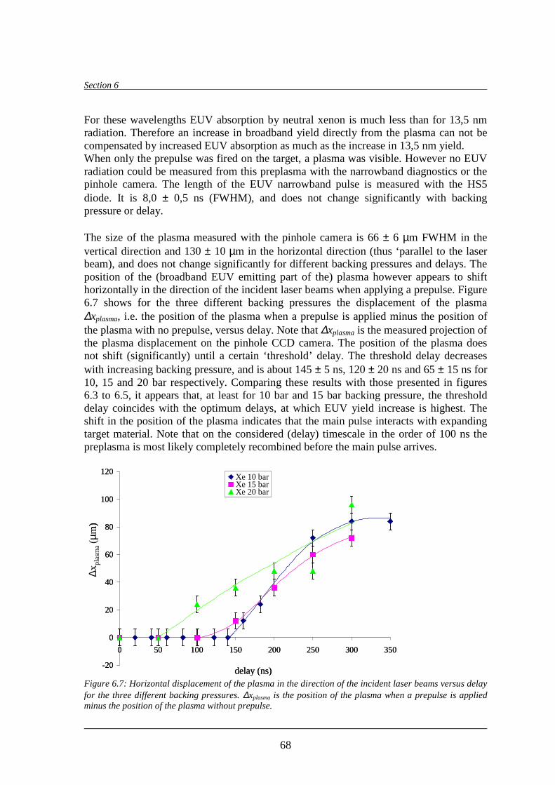
Section 6
68
For these wavelengths EUV absorption by neutral xenon is much less than for 13,5 nm radiation. Therefore an increase in broadband yield directly from the plasma can not be compensated by increased EUV absorption as much as the increase in 13,5 nm yield. When only the prepulse was fired on the target, a plasma was visible. However no EUV radiation could be measured from this preplasma with the narrowband diagnostics or the pinhole camera. The length of the EUV narrowband pulse is measured with the HS5 diode. It is 8,0 ± 0,5 ns (FWHM), and does not change significantly with backing pressure or delay. The size of the plasma measured with the pinhole camera is 66 ± 6 µm FWHM in the vertical direction and 130 ± 10 µm in the horizontal direction (thus ‘parallel to the laser beam), and does not change significantly for different backing pressures and delays. The position of the (broadband EUV emitting part of the) plasma however appears to shift horizontally in the direction of the incident laser beams when applying a prepulse. Figure 6.7 shows for the three different backing pressures the displacement of the plasma ∆xplasma, i.e. the position of the plasma when a prepulse is applied minus the position of the plasma with no prepulse, versus delay. Note that ∆xplasma is the measured projection of the plasma displacement on the pinhole CCD camera. The position of the plasma does not shift (significantly) until a certain ‘ threshold’ delay. The threshold delay decreases with increasing backing pressure, and is about 145 ± 5 ns, 120 ± 20 ns and 65 ± 15 ns for 10, 15 and 20 bar respectively. Comparing these results with those presented in figures 6.3 to 6.5, it appears that, at least for 10 bar and 15 bar backing pressure, the threshold delay coincides with the optimum delays, at which EUV yield increase is highest. The shift in the position of the plasma indicates that the main pulse interacts with expanding target material. Note that on the considered (delay) timescale in the order of 100 ns the preplasma is most likely completely recombined before the main pulse arrives.
-20
0
20
40
60
80
100
120
0 50 100 150 200 250 300 350
delay (ns)
x p
lasm
a (m
)
Xe 10 barXe 15 barXe 20 bar
∆ xpl
asm
a(µ
m)
-20
0
20
40
60
80
100
120
0 50 100 150 200 250 300 350
delay (ns)
x p
lasm
a (m
)
Xe 10 barXe 15 barXe 20 bar
∆ xpl
asm
a(µ
m)
Figure 6.7: Horizontal displacement of the plasma in the direction of the incident laser beams versus delay for the three different backing pressures. ∆xplasma is the position of the plasma when a prepulse is applied minus the position of the plasma without prepulse.
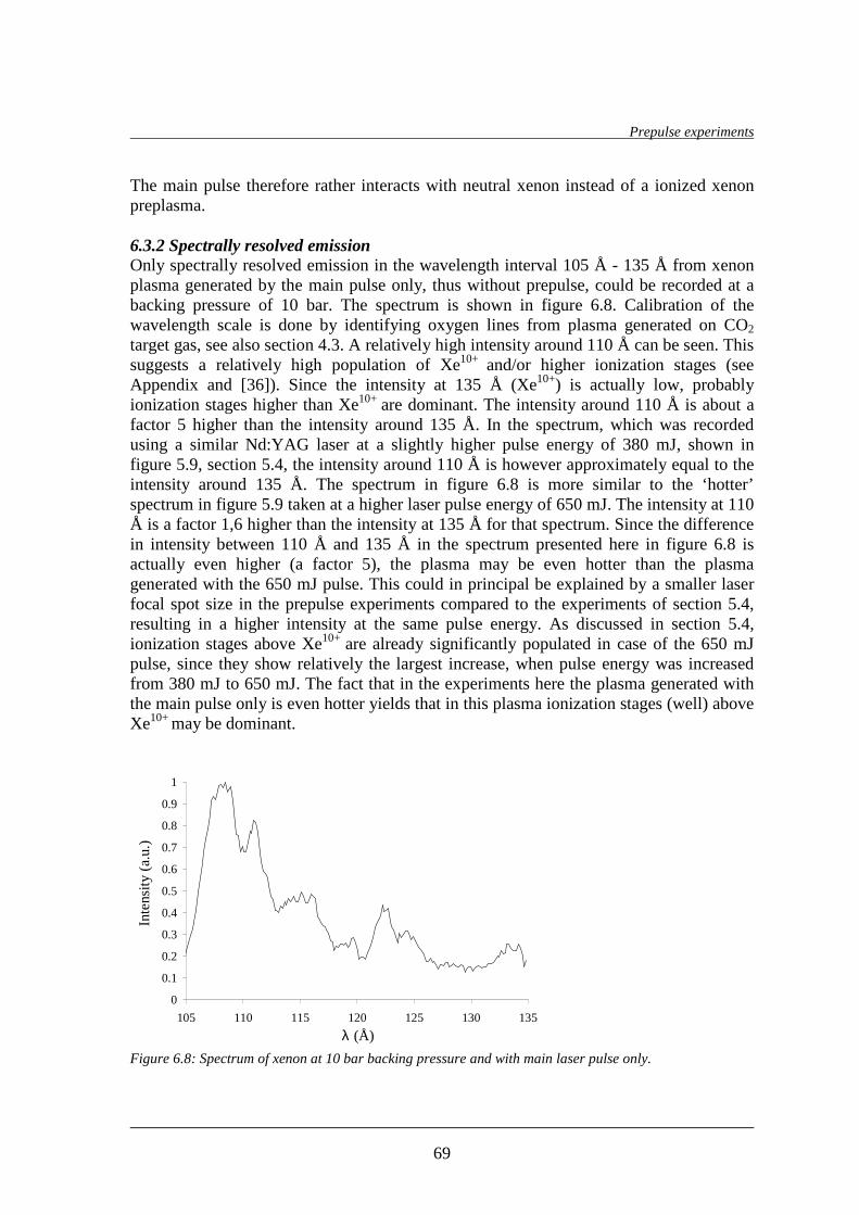
Prepulse experiments
69
The main pulse therefore rather interacts with neutral xenon instead of a ionized xenon preplasma. 6.3.2 Spectrally resolved emission Only spectrally resolved emission in the wavelength interval 105 Å - 135 Å from xenon plasma generated by the main pulse only, thus without prepulse, could be recorded at a backing pressure of 10 bar. The spectrum is shown in figure 6.8. Calibration of the wavelength scale is done by identifying oxygen lines from plasma generated on CO2 target gas, see also section 4.3. A relatively high intensity around 110 Å can be seen. This suggests a relatively high population of Xe10+ and/or higher ionization stages (see Appendix and [36]). Since the intensity at 135 Å (Xe10+) is actually low, probably ionization stages higher than Xe10+ are dominant. The intensity around 110 Å is about a factor 5 higher than the intensity around 135 Å. In the spectrum, which was recorded using a similar Nd:YAG laser at a slightly higher pulse energy of 380 mJ, shown in figure 5.9, section 5.4, the intensity around 110 Å is however approximately equal to the intensity around 135 Å. The spectrum in figure 6.8 is more similar to the ‘hotter’ spectrum in figure 5.9 taken at a higher laser pulse energy of 650 mJ. The intensity at 110 Å is a factor 1,6 higher than the intensity at 135 Å for that spectrum. Since the difference in intensity between 110 Å and 135 Å in the spectrum presented here in figure 6.8 is actually even higher (a factor 5), the plasma may be even hotter than the plasma generated with the 650 mJ pulse. This could in principal be explained by a smaller laser focal spot size in the prepulse experiments compared to the experiments of section 5.4, resulting in a higher intensity at the same pulse energy. As discussed in section 5.4, ionization stages above Xe10+ are already significantly populated in case of the 650 mJ pulse, since they show relatively the largest increase, when pulse energy was increased from 380 mJ to 650 mJ. The fact that in the experiments here the plasma generated with the main pulse only is even hotter yields that in this plasma ionization stages (well ) above Xe10+ may be dominant.
0
0.1
0.2
0.3
0.4
0.5
0.6
0.7
0.8
0.9
1
105 110 115 120 125 130 135
λ (Å)
Inte
nsity
(a.
u.)
Figure 6.8: Spectrum of xenon at 10 bar backing pressure and with main laser pulse only.

Section 6
70
6.4 Discussion Although an increase in EUV yield from the plasma generated with the main pulse is observed when a prepulse is applied, it remains an ongoing discussion in what manner target conditions are precisely changed by the prepulse. Considering the fact that the recombination times in the preplasma, <O(1ns), will be much shorter than the relatively long delay times O(102 ns) between prepulse and main pulse, it can be assumed that the main pulse in any case interacts with neutral xenon target gas. It can therefore be excluded that the increase in EUV yield results from increased inverse Bremsstrahlung absorption of the main laser pulse due to pre-ionization of the target gas (and thus higher initial electron density), as discussed in the second paragraph of subsection 6.1. The prepulse most likely has a gasdynamical effect. Note that the fact that the focal spots of the prepulse and main pulse do not (exactly) coincide may be important in this explanation. The expansion of the preplasma causes a density shockwave, which propagates with a certain velocity v in the surrounding neutral xenon away from the initial preplasma. There is thus a local increase in target gas density in the jet, which propagates through the jet. This is schematically shown in figure 6.9. During a certain time interval after the prepulse the local increase in target gas density propagates through the focus of the main laser pulse. The initial target gas density in the volume with which the main pulse interacts is then (partly) increased. As discussed extensively in section 5 (subsection 5.2 in particular), an increase in initial target gas density will result in enhanced EUV emission directly from the plasma generated by the main pulse. Since the gas density in the region surrounding the main pulse plasma does not (necessarily) increase, the EUV absorption by neutral gas in the jet remains the same. The increase in EUV emission will start as soon as the shockwave gets in the focal spot of the main pulse, and will be maximum if the main pulse focal spot completely ‘contains’ the density shock. If the shockwave leaves the focal spot, the EUV yield will decrease again.
position →
targ
et g
as d
ensi
ty→
density shock wavev
prepulse focal spot main pulse focal spot
Figure 6.9: Schematic one dimensional representation of the density shockwave propagating through the gas jet. The shockwave moves away from the prepulse focal spot (where the preplasma is formed). Due to the increased target gas density, the EUV yield from the main laser pulse plasma increases as soon as the shockwave arr ives at the main pulse focal spot. The yield increase is the highest when the focal spot completely contains the density shock. The EUV yield decreases again as soon as the shockwave leaves the main pulse focal spot.

Prepulse experiments
71
This explains thus the dependence of the EUV yield increase on the delay between prepulse and main pulse, cf f igures 6.3 to 6.5. Note that the observed maximum yield increase by about a factor 2,5 yields a (average) density increase by a factor √(2,5) = 1,6. From figures 6.3 to 6.5 also the velocity of the density shockwave can be estimated roughly. The time interval in which a EUV yield increase is observed is about 200 ns to 300 ns. According to the discussion above the density shockwave propagates through the main pulse focal spot during this time interval. Taking the focal spot size of ~30 µm then gives a shockwave velocity of ~102 m/s. As should be expected this is in the order of the sound of speed in the gas jet. From equation (3.2) it can namely be calculated that the sound of speed is Vs = 63 m/s at the nozzle’s exit, using γ = 5/3, M = 4,5 (see subsection 3.1), and the speed of sound in xenon Vs,0 = 176 m/s at 295 K. Note that the actual orientation of the two laser beams and the EUV diagnostics with respect to each other in the experiment complicates the discussion above, which is basically a 1-dimensional sketch of the situation. For instance the fact that measured broadband yield decreases for delays longer than ~250 ns when using the prepulse may be explained by an increase in xenon density (and thus EUV absorption) between the main pulse plasma and the pinhole camera due to the shockwave. Also the fact that the position of the main pulse plasma shifts above certain delays when using the prepulse may be because the shockwave changes the position at which the main pulse interacts with the target gas. Note that from the slopes of the graphs in figure 6.7 the velocity of the shift in plasma position is in the order of several times 102 m/s, and thus higher than the shockwave velocity of ~102 m/s estimated in the discussion above.

Conclusion
72
Conclusion
In this study three different experiments concerning a laser plasma EUV source based on a supersonic xenon gas jet target are performed. Firstly a backlighting technique is used to determine the initial gas mass density in the supersonic xenon jet. Shadowgraphs of the gas jet are recorded, giving the absorption (profile) of keV radiation from a solid target laser plasma passing through the gas jet. From these shadowgraphs the gas mass density profile in the jet can in principle be deduced by using an inverse Abel transform. Although no density profiles are calculated and presented (yet) in this report, the shadowgraphs are in first instance compared with absorption profiles expected from Laval nozzle theory. Especially the shadowgraphs of the large nozzle used in this study appear to be in good agreement with theory. The shadowgraphs of the small nozzle display a larger deviation from theory at the edges of the jet, indicating that the density profile is not flat (as in theory) and that the density at the edges of the jet is lower than in theory. Secondly, to increase the understanding of the relevant processes in the gas jet laser plasma EUV source, a parameter study is performed, in which spectrally resolved EUV emission from laser plasma generated on the supersonic xenon jet is investigated for different laser pulse intensities and initial target gas densities (known from backlighting). A KrF excimer laser and a Nd:YAG laser with intensities in the order of 1012 Wcm-2 and 1013 Wcm-2 respectively are used. Spectra of KrF laser plasmas indicate that the highest ionization stage significantly populated is Xe9+ (whereas Xe10+ is needed for high 13,5 nm EUV emission). Spectra of Nd:YAG laser plasmas show a relatively larger line emission corresponding with Xe10+ transitions. Ionization stages above Xe10+ are significantly populated in these plasmas. The measured dependence of spectral intensity on initial target gas density is quantitatively explained by a theoretical model. The model makes a distinction between the spectral intensity directly from the EUV emitting plasma and the transmission of the EUV radiation through the neutral (and weakly ionized) gas in the jet surrounding the plasma. By applying coronal equili brium (which is justified for the concerning plasmas), and by assuming that the electron temperature and plasma size do not depend on target gas density (the latter assumption is confirmed by pinhole camera measurements), it is found that the spectral intensity directly from the plasma is proportional to the initial target gas density squared. An additional increase in spectral intensity measured when increasing target gas density is explained by a small electron temperature increase of less than 9%. However the increase in intensity from the plasma when increasing target gas density is ‘ counter acted’ by an increase in absorption by the surrounding neutral xenon. By using the fact that the absorption coeff icient of xenon surrounding the plasma is proportional to the target gas density, a ‘self’ absorption of about 70% and 90% is found for the large nozzle at 10 bar rep. 20 bar backing pressure. Finally, increasing the conversion efficiency from laser light into EUV radiation, by applying a laser prepulse, which modifies initial target conditions, prior to the laser main pulse, is investigated experimentally. An increase in 13,5 nm EUV narrowband and 6-16 nm EUV broadband emission is found for time delays between pre- and main pulse up to 250 ns. A maximum narrowband yield and broadband yield increase by a factor 2,5 resp. 1,8 is found at a delay of 140 ns when applying the prepulse. Considering the large time delays between the two laser pulses, the prepulse most likely has a gasdynamical effect; The laser prepulse causes a density shockwave propagating in the xenon gas jet. The resulting local increase in target gas density at the main laser pulse focal spot (during a certain time delay interval) gives the observed enhancement of EUV emission.

Acknowledgements
73
Acknowledgements I would like to thank my attendant Rene de Bruijn and the other LPX-colleagues at FOM Rijnhuizen: Konstantin Koshelev, Evert Wagner, Elena Toma, Remko Stuik, Fred Bijkerk and the muco-people. Furthermore I would like to thank Joost van der Mullen, Erik Kieft and Kurt Garloff f or useful discussions and suggestions. Thanks go to Graeme Hirst, Waseem Shaikh, Andrew Bodey and all the other people at RAL who have supported the prepulse experiments, and to Serguei Zakharov and Vladimir Ivanov for discussing the results. Also thanks go to Serguei Churilov for providing spectral data of xenon.

References
74
References
[1] X-rays from laser plasmas, generation and applications; I.C.E. Turcu, J.B. Dance; Wiley, 1999; ISBN 0 471 98397 7.
[2] Making ultrabright X-rays; M. Altarelli , F. Schlachter, J. Cross; Scientific American, december 1998.
[3] Soft X-ray optics; E. Spill er; SPIE Optical Engineering Press, 1994; ISBN 0 81941 654 1.
[4] Multil ayer coatings - a mini-tutorial: http://www-cxro.lbl.gov/multil ayer/mltutor.html
[5] Progress in Mo/Si multilayer coating technology for EUVL optics; E. Louis et al.; SPIE 3997 (Micro Lithography), Santa Clara, 2000
[6] C. Montcalm, S. Bajt, P. Mirkarimi, E. Spiller, F. Weber, J. Folta; SPIE Vol. 3331 1998.
[7] Mo/Si multilayer coating technology for EUVL, coating uniformity and time stabili ty; E. Louis et al.; SPIE 4146-06, Soft X-ray and EUV Imaging Systems, San Diego, 2000.
[8] Developments of a high-power, low-contamination laser plasma source for EUV projection lithography; L.A. Shmaenok et al.; SPIE Vol. 2523, 1995.
[9] Demonstration of a foil trap technique to eliminate laser plasma atomic debris and small particulates; L.A. Shmaenok et al.; SPIE 3331, 1998.
[10] X-ray emission from laser irradiated gas puff targets; H. Fiedorowicz, A. Bartnik, Z. Patron; Appl. Phys. Lett. 62 (22), pp. 1-3, 1993.
[11] High-power extreme ultraviolet source based on gas jets; G.D. Kubiak, L. J. Bernardez, K. Krenz; SPIE 3331, p.81-89, 1998.
[12] Characterization of a novel double-jet laser-plasma EUV source; R. de Bruijn et al.; SPIE 3997, p.157, 2000.
[13] Enhanced X-ray emission in the 1-keV range from a laser irradiated gas-puff target produced using the double-nozzle setup; H. Fiedorowicz et al.; Appl. Phys. B 70, 1-4, 2000.
[14] Inleiding Plasmafysica; D.C. Schram, M.C.M. van de Sanden; Technische Universiteit Eindhoven, Faculteit Technische Natuurkunde, 1997.
[15] Handbook of Chemistry and Physics 76th edition, 10-207; CRC press Inc., 1995. [16] Laser-induced breakdown phenomena; C. Grey Morgan; Sci. Prog. Oxf. 65, p31-50,
1978. [17] Laser ionization and heating of gas targets for long-scale-length instabili ty
experiments; J. Denavit, D.W. Philli on; Phys. Plasmas 1 (6), p.1971-1984, june 1994.
[18] Ionization in the field of a strong electromagnetic field; L.V. Keldysh; Soviet Physics JETP, vol.20, no.5, may 1965.
[19] Cluster explosions and characterization of ultrashort XUV pulses; E. Toma; PhD. thesis 2002; ISBN 90-9015483-3.
[20] Plasmas and laser light; T.P. Hughes; Adam Hilger Ltd., 1975; ISBN 0 85274 086 7.

References
75
[21] Correct values for high-frequency power absorption by inverse bremsstrahlung in plasmas; T.W. Johnston, J.M. Dawson; The Physics of Fluids, vol.16, no. 5, may 1973.
[22] A simple model for laser-produced, mass-limited water droplet plasmas; K. Garloff, M. van den Donker, J. van der Mullen, F. van Goor, R. Brummans, J. Jonkers; to be published.
[23] Gasdynamica; M.E.H. van Dongen; Technische Universiteit Eindhoven, Faculteit Technische Natuurkunde, 2001.
[24] Compressible fluid dynamics; Patrick H. Oosthuizen, Willi am E. Carscallen; McGraw-Hill , 1997; ISBN 0-07-048197-0.
[25] Auflösung einer mechanischen Aufgabe; N. H. Abel; J. Reine und Angew. Math., 1:153-157, 1826.
[26] Characterization of neutral density profile in a wide range of pressure of cylindrical pulsed gas jets; V. Malka et al.; Review of Scientific Instruments, vol.71, no.6, june 2000.
[27] X-ray interactions with matter: http://www-cxro.lbl.gov/optical_constants/ [28] MIE-scattering experiments, R. de Bruijn. [29] Principles of Optics; M. Born, E. Wolf; Pergamon press ltd., 3rd edition, 1965. [30] Atomic and Ionic Spectrum Lines Below 2000 Å, H through Ar; R. L. Kelly; Oak
Ridge National Laboratory, 1982. [31] Diffraction grating transmission eff iciencies for XUV and soft X-rays; H. W.
Schnopper et al.; Applied Optics, Vol. 16, No. 4, April 1977. [32] Cd I isoelectric sequence: wavelengths and energy levels for Xe VII through Eu
XVI; V. Kaufman, J. Sugar; J. Opt. Soc. Am. B, Vol. 4, No.12, December 1987. [33] Analysis of the 4p64d84f and 4p54d10 configurations of Xe X and some highly
excited levels of Xe VIII and Xe IX ions; S. S. Churilov, Y. N. Joshi; Physica Scripta, Vol. 65, 40-45, 2002.
[34] Private communication; S. S. Churilov. [35] Revised NRL Plasma Formulary:
http://wwwppd.nrl.navy.mil/nrlformulary/nrlformulary.html [36] Highly ionized xenon spectra (95-260 Å) excited in TFR tokamak plasmas; C.
Breton et al.; Physica Scripta, vol. 37, p33-37, 1988. [37] A plasma light source for the VUV spectral region; W. Shaikh; IEEE journal of
quantum electronics, Vol.5, no.6, Nov/Dec 1999. [38] Enhancement of keV X-ray emission in laser-produced plasmas by a weak prepulse
laser; R. Kodama, T. Mochizuki, K.A. Tanaka, C. Yamanaka; Appl. Phys. Lett., vol. 50, no.12, 23 March 1987.
[39] Enhancement of soft X-ray emission using prepulses with 2ω and 4ω laser plasmas; K.A. Tanaka et al.; J. Appl. Phys. 63 (5), 1 March 1988.
[40] Soft X-ray emission from double-pulse laser-produced plasma; R. Weber, J.E. Balmer; J. Appl. Phys. 65 (5), 1 March 1989.
[41] The interaction of a high irradiance, subpicosecond laser pulse with aluminium: The effects of the prepulse on X-ray production; J. A. Cobble et al.; J. Appl. Phys. 69 (5), 1 March 1991.

References
76
[42] Prepulse-enhanced narrow bandwidth soft X-ray emission from a low debris, subnansecond, laser plasma source; P. Dunne, G. O’Sulli van, D. O’Reil ly; Appl. Phys. Lett. vol. 76, no.1, 3 January 2000.
[43] Ultraviolet prepulse for enhanced X-ray emission and brightness from droplet-target laser plasmas; M. Berglund, L. Rymell , H.M. Hertz; Appl. Phys. Lett. 69 (12), 16 September 1996.
[44] Plasma and XUV source characteristics for Al targets heated by 40 ns Nd-laser pulses; R.R. Whitlock, J.R. Greig, D.J. Nagel, S.J. Topscher; J. Vac. Sci. Technol. B 19(4), Juli/August 2001.
[45] X-ray emission in laser-produced plasmas; D. Colombant, G.F. Tonon; J. Appl. Phys., vol. 44, no. 8, p.3524-3537, August 1973.
[46] Spectra of Xe VII, VII I, and IX in the extreme ultraviolet: 4d-mp, nf transitions; J. Blackburn, P.K. Carroll , J. Costello, G. O’Sulli van; J. Opt. Soc. Am., vol. 73, no. 10, October 1983.
[47] Calibration of Flying Circus EUV diagnostics; R. Stuik, F. Bijkerk; Nuclear Instruments and Methods A, submitted 2002.
[48] Linearity of P-N junction photodiodes under pulsed irradiation; R. Stuik, F. Bijkerk; SPIE, vol. 4688, 2002.

Appendix
77
Appendix Spectral data of Xe6+ to Xe10+
Spectral li nes of Xe6+ to Xe10+ below 200 Å are given in tables A.1 to A.5 respectively. Data of Xe6+ is from [32], data of Xe7+, Xe8+ and Xe9+ is from [33], data of Xe10+ is from [34]. The tables also give the corresponding transition and transition probabili ty gA (equal to Aqp defined in eq. (2.45)). Note that also some lines of O4+ and O5+ are given in the tables. Table A.1: Spectral li nes of XeVII (Xe6+) below 200 Å. Data is from [32] . The 4d9 5s2 5p and 4d9 5s2 4f configurations are designed as d5p and d4f.
λ (Å) transition gA (109s-1) I 123.242 5s2 1S0 - d4f 1P1 6645.0 30? 181.876 5s2 1S0 - d5p 3D1 37.2 20 185.438 5s2 1S0 - d5p 1P1 222.5 50
Table A.2: Spectral li nes of XeVIII (Xe7+) below 200 Å. Data is from [33] . Configuration designations: sp = 4d9 5s5p, sf = 4d9 5s4f.
λ (Å) transition gA (109s-1) I
123.243 5s 2S 0.5 - sf 2P 1.5 20 123.265 5s 2S 0.5 - sf 2P 0.5 15 166.671 5s 2S 0.5 - sp 2Pb0.5 32 170.861 5s 2S 0.5 - sp 2Pb1.5 37 174.155 5s 2S 0.5 - sp 4D 1.5 4 175.886 5s 2S 0.5 - sp 4D 0.5 6 177.271 5s 2S 0.5 - sp 2Pa0.5 30 177.721 5s 2S 0.5 - sp 2Pa1.5 38 179.669 5s 2S 0.5 - sp 2Da1.5 14 180.129 5s 2S 0.5 - sp 4P 0.5 8 181.682 5s 2S 0.5 - sp 4F 1.5 6 184.665 5s 2S 0.5 - sp 4P 1.5 6
Table A.3: Spectral li nes of XeIX (Xe8+) below 200 Å. Data is from [33] . ? indicates tentative classification
λ (Å) transition gA (109s-1) I
168.202 1S0-5p 3P1 0.2 ? 165.323 ‘ ‘ 1P1 241 100 161.742 ‘ ‘ 3D1 45 70
150.274 ? 1S0-4f 3P1 1 2 143.614 ‘ ‘ 3D1 6 10 120.133 ‘ ‘ 1P1 4554 40
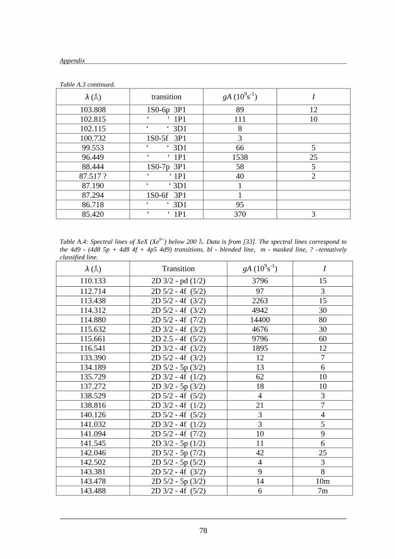
Appendix
78
Table A.3 continued.
λ (Å) transition gA (109s-1) I
103.808 1S0-6p 3P1 89 12 102.815 ‘ ‘ 1P1 111 10 102.115 ‘ ‘ 3D1 8 100.732 1S0-5f 3P1 3 99.553 ‘ ‘ 3D1 66 5 96.449 ‘ ‘ 1P1 1538 25 88.444 1S0-7p 3P1 58 5
87.517 ? ‘ ‘ 1P1 40 2 87.190 ‘ ‘ 3D1 1 87.294 1S0-6f 3P1 1 86.718 ‘ ‘ 3D1 95 85.420 ‘ ‘ 1P1 370 3
Table A.4: Spectral li nes of XeX (Xe9+) below 200 Å. Data is from [33] . The spectral li nes correspond to the 4d9 - (4d8 5p + 4d8 4f + 4p5 4d9) transitions. bl - blended line, m - masked line, ? –tentatively classified line.
λ (Å) Transition gA (109s-1) I
110.133 2D 3/2 - pd (1/2) 3796 15 112.714 2D 5/2 - 4f (5/2) 97 3 113.438 2D 5/2 - 4f (3/2) 2263 15 114.312 2D 5/2 - 4f (3/2) 4942 30 114.880 2D 5/2 - 4f (7/2) 14400 80 115.632 2D 3/2 - 4f (3/2) 4676 30 115.661 2D 2.5 - 4f (5/2) 9796 60 116.541 2D 3/2 - 4f (3/2) 1895 12 133.390 2D 5/2 - 4f (3/2) 12 7 134.189 2D 5/2 - 5p (3/2) 13 6 135.729 2D 3/2 - 4f (1/2) 62 10 137.272 2D 3/2 - 5p (3/2) 18 10 138.529 2D 5/2 - 4f (5/2) 4 3 138.816 2D 3/2 - 4f (1/2) 21 7 140.126 2D 5/2 - 4f (5/2) 3 4 141.032 2D 3/2 - 4f (1/2) 3 5 141.094 2D 5/2 - 4f (7/2) 10 9 141.545 2D 3/2 - 5p (1/2) 11 6 142.046 2D 5/2 - 5p (7/2) 42 25 142.502 2D 5/2 - 5p (5/2) 4 3 143.381 2D 5/2 - 4f (3/2) 9 8 143.478 2D 5/2 - 5p (3/2) 14 10m 143.488 2D 3/2 - 4f (5/2) 6 7m

Appendix
79
Table A.4 continued.
λ (Å) Transition gA (109s-1) I 143.954 2D 3/2 - 4f (5/2) 3 2 144.079 2D 5/2 - 5p (5/2) 5 2 144.655 2D 5/2 - 5p (3/2) 25 20 144.771 2D 5/2 - 5p (5/2) 14 7 145.096 2D 5/2 - 4f (3/2) 19 5 145.150 2D 3/2 - 5p (1/2) 201 35 145.325 2D 5/2 - 5p (3/2) 94 25 145.397 2D 5/2 - 4f (7/2) 3 4 145.715 2D 5/2 - 4f (5/2) 3 4 145.788 2D 3/2 - 4f (1/2) 2 3 145.983 2D 3/2 - 5p (5/2) 181 55 146.107 2D 3/2 - 4f (5/2) 16 17 146.148 2D 5/2 - 5p (7/2) 10 8 146.413 2D 5/2 - 5p (3/2) 24 15 146.448 2D 5/2 - 5p (5/2) 13 5 146.532 2D 5/2 - 4f (3/2) 16 4 146.622 2D 3/2 - 4f (5/2) 11 5 147.005 2D 3/2 - 5p (3/2) 5 2 147.381 2D 3/2 - 5p (1/2) 19 8 147.418 2D 5/2 - 4f (5/2) 6 6 147.618 2D 5/2 - 5p (3/2) 226 72 147.640 2D 3/2 - 5p (5/2) 66 34 147.734 2D 5/2 - 4f (7/2) 13 6 147.956 2D 5/2 - 5p (7/2) 321 100 148.005 2D 5/2 - 5p (5/2) 143 56 148.238 2D 3/2 - 5p (3/2) 16 10 148.333 2D 5/2 - 5p (3/2) 52 30 148.359 2D 3/2 - 5p (5/2) 129 52 148.641 2D 5/2 - 5p (7/2) <0.1 6? 148.709 2D 3/2 - 4f (3/2) 48 23 148.942 2D 3/2 - 5p (3/2) 133 44 149.020 2D 5/2 - 5p (5/2) 133 75 149.358 2D 5/2 - 5p (7/2) 195 80 149.583 2D 5/2 - 5p (5/2) 66 42 149.682 2D 3/2 - 4f (1/2) 9 4 150.089 2D 3/2 - 5p (3/2)
O VI 242 150bl
150.124
2D 3/2 - 5p (5/2) O VI
56 95bl
150.216 2D 3/2 - 4f (3/2) 26 5 150.444 2D 3/2 - 5p (1/2) 14 9 150.544 2D 5/2 - 5p (5/2) 238 90 151.020 2D 5/2 - 5p (3/2) 13 10

Appendix
80
Table A.4 continued. λ (Å) Transition gA (109s-1) I
151.141 2D 3/2 - 4f (5/2) 7 9 151.291 2D 3/2 - 5p (1/2) 8 6 151.356 2D 3/2 - 5p (3/2) 7 4 151.747 2D 5/2 - 5p (7/2) 86 80 151.762 2D 3/2 - 5p (5/2) 40 27 152.058 2D 5/2 - 5p (5/2) 110 78 152.832 2D 3/2 - 5p (5/2) 13 6 152.849 2D 5/2 - 5p (3/2) 4 5 154.433 2D 3/2 - 5p (5/2) 12 6 154.588 2D 5/2 - 5p (7/2) 3 8 154.680 2D 5/2 - 5p (5/2) 19 24 154.935 2D 3/2 - 5p (3/2) 13 15 155.248 2D 5/2 - 5p (3/2) 2 4 156.300 2D 3/2 - 5p (1/2) 1 3 156.857 2D 3/2 - 5p (3/2) 2 5 158.924 2D 5/2 - pd (3/2) 12 7 158.972 2D 5/2 - 5p (7/2) 2 3 159.388 2D 3/2 - 5p (3/2)
O V 5 10m
163.262 2D 3/2 - pd (3/2) 2 3 Table A.5: Spectral li nes of XeXI (Xe10+) below 200 Å. Data is from [34] . The lines correspond to the 4p6_4d8 - (4p6_4d7_5p + 4p6_4d7_4f + 4p5_4d9) transitions.
λ (Å) Transition gA (109s-1) I
105.198 1D2 - 4f (1) 127 107.242 3F3 - pd (2) 32 108.411 3P1 - pd (2) 45 108.472 1G4 - pd(3) 69 108.572 3P2 - pd (2) 52 108.724 1D2 - pd (3) 34 109.409 1D2 - pd (2) 147bl 109.488 3P1 - pd (2) 85 110.289 1D2 - 4f (1) 47 110.408 1S0 - 4f (1) 37 110.997 3F2 - 4f (2) 23 110.515 1D2 - pd (2) 70 111.120 3F3 - 4f (3) 112 111.262 3F3 - 4f (2) 20 111.290 3P1 - 4f (1) 28 111.385 1G4 - 4f (5) 139 111.434 3F4 - 4f (3) 133 111.490 3F2 - 4f (2) 40
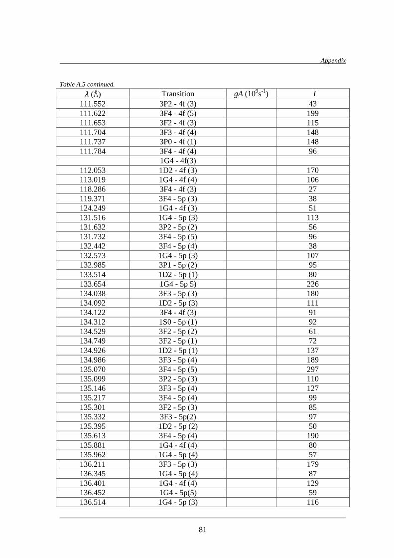
Appendix
81
Table A.5 continued.
λ (Å) Transition gA (109s-1) I 111.552 3P2 - 4f (3) 43 111.622 3F4 - 4f (5) 199 111.653 3F2 - 4f (3) 115 111.704 3F3 - 4f (4) 148 111.737 3P0 - 4f (1) 148 111.784 3F4 - 4f (4) 96
1G4 - 4f(3) 112.053 1D2 - 4f (3) 170 113.019 1G4 - 4f (4) 106 118.286 3F4 - 4f (3) 27 119.371 3F4 - 5p (3) 38 124.249 1G4 - 4f (3) 51 131.516 1G4 - 5p (3) 113 131.632 3P2 - 5p (2) 56 131.732 3F4 - 5p (5) 96 132.442 3F4 - 5p (4) 38 132.573 1G4 - 5p (3) 107 132.985 3P1 - 5p (2) 95 133.514 1D2 - 5p (1) 80 133.654 1G4 - 5p 5) 226 134.038 3F3 - 5p (3) 180 134.092 1D2 - 5p (3) 111 134.122 3F4 - 4f (3) 91 134.312 1S0 - 5p (1) 92 134.529 3F2 - 5p (2) 61 134.749 3F2 - 5p (1) 72 134.926 1D2 - 5p (1) 137 134.986 3F3 - 5p (4) 189 135.070 3F4 - 5p (5) 297 135.099 3P2 - 5p (3) 110 135.146 3F3 - 5p (4) 127 135.217 3F4 - 5p (4) 99 135.301 3F2 - 5p (3) 85 135.332 3F3 - 5p(2) 97 135.395 1D2 - 5p (2) 50 135.613 3F4 - 5p (4) 190 135.881 1G4 - 4f (4) 80 135.962 1G4 - 5p (4) 57 136.211 3F3 - 5p (3) 179 136.345 1G4 - 5p (4) 87 136.401 1G4 - 4f (4) 129 136.452 1G4 - 5p(5) 59 136.514 1G4 - 5p (3) 116

Appendix
82
Table A.5 continued λ (Å) Transition gA (109s-1) I
136.605 3F4 - 5p (4) 151 136.916 1D2 - 5p (3) 35 137.237 3F2 - 5p (3) 102 137.778 3F4 - 4f (3) 68 138.458 1G4 - 5p (4) 132 138.934 3P1 - 5p (2) 55 139.175 1G4 - 5p (5) 92 140.294 3F2 - 4f (3) 35


![[New Symmetry Issue] Xenon, Xenon Everywhere; A Measurement to Watch](https://img.pdfslide.us/doc/110x75/563db844550346aa9a9221ed/new-symmetry-issue-xenon-xenon-everywhere-a-measurement-to-watch.jpg)