Embed Size (px)
Citation preview
A LARGE SCALE SIMULATION OF SATELLITES TRACKING VESSELS
AND OTHER TARGETS
SRIYAN INDRAJITH WISNARAMA
A THESIS SUBMITTED TO THE FACULTY OF GRADUATE STUDIES IN
PARTIAL FULFILLMENT OF THE REQUIREMENTS FOR THE DEGREE OF
MASTER OF SCIENCE
GRADUATE PROGRAM IN EARTH AND SPACE SCIENCE
YORK UNIVERSITY
TORONTO, ONTARIO
April 2014
© SRIYAN INDRAJITH WISNARAMA 2014
ii
Abstract
This research outlines the design of a large scale simulation of satellites tracking large amounts of
dynamic targets. The use of such a simulation is presented and current solutions available are presented.
The research sets out a list of objectives to meet by creating an application programming interface (API)
that have the requirements of being efficient, scalable, flexible, and easy to use for the implementer.
Methods of creating sections of the simulation such as the attitude motion of a satellite based on the
physical characteristics of nanosatellites is explored and developed. The creation of targets that are
contained only on certain land features are also developed and tested. The objectives set out are tested by
creating a simulation using the API developed and the results are presented.
iii
Acknowledgements
I would first like to thank all the people at York University for their continued help and encouragement. I
would first like to thank my supervisor Dr. Regina Lee for taking a chance with accepting me as her
student - without her guidance, motivation, and belief in me, this research would not be possible. I would
also like to thank COM DEV and McMaster University for providing me the opportunity to be part of
their research project. It has been a very unique experience and would be my first step into working in
collaborative projects.
I would like to thank my fellow colleagues for all the laughs and help they have provided, especially to
the people on the fourth floor of Petrie. I would also like to thank Kavita Joshi for helping me stay
focused and always believing in me. Finally, I would like to thank my family, my parents for giving me
all that I have and my sister in helping edit my work.
iv
Table of Contents
ABSTRACT ................................................................................................................................................ II
ACKNOWLEDGEMENTS .................................................................................................................... III
LIST OF TABLES ................................................................................................................................ VIII
LIST OF FIGURES .................................................................................................................................. IX
CHAPTER 1 – INTRODUCTION ............................................................................................................ 1
1.1 MOTIVATION .......................................................................................................................... 2
1.2 RESEARCH OBJECTIVES.......................................................................................................... 3
1.3 APPLICATIONS OF SATELLITE TARGET TRACKING SIMULATION ........................................... 4
1.3.1 Application in Mission Design ....................................................................................... 5
1.3.2 Mission Operations ......................................................................................................... 7
1.3.3 Growing Needs of Satellite AIS ...................................................................................... 9
1.4 SATELLITE GEOLOCATION ................................................................................................... 10
1.4.1 Location Determination vs. Orbit Determination ......................................................... 10
1.4.2 Satellite Tracking vs. Tracking Satellites ..................................................................... 10
1.4.3 Use of Satellite Geolocation ......................................................................................... 12
1.5 THESIS OUTLINE ................................................................................................................... 13
CHAPTER 2 – BACKGROUND ............................................................................................................. 15
2.1 TRACKING FROM A SATELLITE ............................................................................................. 15
2.1.1 Animal Tracking ........................................................................................................... 15
2.1.2 Human Tracking ........................................................................................................... 17
2.1.3 Vehicular and Aircraft Traffic ...................................................................................... 18
v
2.1.4 Vessel Tracking ............................................................................................................ 19
2.2 SATELLITE GEOLOCATION METHODS .................................................................................. 21
2.2.1 Satellite Laser Ranging ................................................................................................. 21
2.2.2 Radar ............................................................................................................................. 21
2.2.3 Optical Methods ............................................................................................................ 22
2.2.4 GPS and Other Onboard Systems ................................................................................. 24
2.3 SATELLITE AUTOMATIC IDENTIFICATION SYSTEM (AIS) DETECTION ................................ 26
2.3.1 History and Function of the Automatic Identification System (AIS) ........................... 26
2.3.2 Space-based AIS tracking providers ............................................................................. 28
2.4 COORDINATE SYSTEMS ........................................................................................................ 29
CHAPTER 3 – DEVELOPMENT OF APPLICATION PROGRAMMING INTERFACE FOR
THE SIMULATION ................................................................................................................................. 30
3.1 COMMERCIAL/ OPEN SOURCE APIS AND SIMULATION........................................................ 30
3.2 APPLICATION PROGRAMMING INTERFACE (API) MODELS .................................................. 31
3.2.1 Spherical Earth and Circular Orbit API ........................................................................ 31
3.2.2 Single Satellite Non-Spherical Earth and Non-Circular Orbit API............................... 35
3.2.3 Multi-Satellite and Database API ................................................................................. 36
CHAPTER 4 – SATELLITE ATTITUDE CONTROL ........................................................................ 40
4.1 SATELLITE ATTITUDE DETERMINATION AND ATTITUDE CONTROL .................................... 40
4.2 Attitude Determination .................................................................................................... 41
4.3 Attitude Control ............................................................................................................... 42
4.4 SATELLITE MODEL ............................................................................................................... 42
4.4.1 External Torques ........................................................................................................... 42
4.4.2 The Control System Used to Simulate Attitude ............................................................ 44
vi
4.5 SUMMARY ............................................................................................................................ 48
CHAPTER 5 – GROUND/AIR TARGET DATA .................................................................................. 50
5.1 ARTIFICIAL POINT GENERATION .......................................................................................... 50
5.1.1 ArcGIS .......................................................................................................................... 51
5.2 REAL WORLD TARGET DATA ............................................................................................... 52
5.3 SIMULATED SOURCES OF DATA ........................................................................................... 53
CHAPTER 6 – SIMULATION API FEATURES AND TEST RESULTS .......................................... 55
6.1 SCALABILITY AND FLEXIBILITY ........................................................................................... 55
6.1.1 Efficiency ...................................................................................................................... 56
6.2 GRAPHICAL USER INTERFACE .............................................................................................. 58
6.3 TESTING AND RESULTS ........................................................................................................ 60
6.4 LIMITATIONS ........................................................................................................................ 68
CHAPTER 7 – FUTURE WORK AND CONCLUSION ...................................................................... 70
7.1 FUTURE WORK ..................................................................................................................... 70
7.1.1 Transmitter Modelling and Receiver Modelling ........................................................... 70
7.1.2 Artificial Target Generation .......................................................................................... 70
7.1.3 GUI Improvement ......................................................................................................... 71
7.2 FINAL REMARKS................................................................................................................... 72
7.3 CONTRIBUTIONS ................................................................................................................... 73
BIBLIOGRAPHY ..................................................................................................................................... 76
APPENDIX ................................................................................................................................................ 84
APPENDIX A – STK ATTITUDE FILE .......................................................................................... 84
APPENDIX B – LANGUAGES AND APIS ...................................................................................... 85
vii
APPENDIX C – MISSION OPERATIONS CONTROLLERS ............................................................... 85
APPENDIX D – LIST OF ACRONYMS ........................................................................................... 89

viii
List of Tables
Table 1: Mission Operations Controllers ......................................................................................... 8
ix
List of Figures
Figure 1: The simulated scenario of AIS signal detection from space [6] .................................................... 7
Figure 2: Satellite Tracking, showing a satellite tracking ground targets ................................................... 11
Figure 3: Tracking Satellite, showing that a satellite is being tracked using many different methods ....... 12
Figure 4: Platform Transmitter Terminal (PPT) Device that Attaches to a Bird [16] ................................ 16
Figure 5: Aireon's Global Coverage Compared with Current Coverage. The orange represents the areas of
coverage. [26] ............................................................................................................................................. 19
Figure 6: NTS Nanosatellite [28] ................................................................................................................ 20
Figure 7: PAVE PAWS Radar in Alaska [30] ............................................................................................ 22
Figure 8: Baker-Nunn Telescope [32] ........................................................................................................ 23
Figure 9: Maui Space Surveillance Site [33] .............................................................................................. 24
Figure 10: Cube-Sat based GPS receiver at the low end of cost at $19,700 [34] ....................................... 25
Figure 11: A higher-end GPS receiver with cost at $277,100 [34] ............................................................. 25
Figure 12: Typical AIS Transceiver Sold to the Public [39] ...................................................................... 27
Figure 13: This Shows How Signals from Ships Avoid Overlapping by Using SOTDMA [6] ................. 28
Figure 14: Interior Angle α Corresponding to FOV Angle θ ...................................................................... 32
Figure 15: Interior Angle Distortion due to Attitude Change ..................................................................... 33
Figure 16: Class Hierarchy ......................................................................................................................... 37
Figure 17: IMU on a PCB [48] ................................................................................................................... 41
Figure 18: Earth's Magnetic Field Direction [49] ....................................................................................... 44
Figure 19: NTS shown with Roll Pitch Yaw Diagram [51] ........................................................................ 45
Figure 20: Differential Equation of Plant ................................................................................................... 45
Figure 21: Satellite Plant in the s-domain ................................................................................................... 46
x
Figure 22: Overall Block Diagram of the Attitude Determination and Control System ............................. 46
Figure 23: Simplified Block Diagram of Control System .......................................................................... 47
Figure 24: Simulink® Diagram of System Block Diagram ......................................................................... 48
Figure 25: 10,000 ships randomly generated on a spherical Earth ............................................................. 51
Figure 26: Points (green) only on oceans in ArcMap ................................................................................. 52
Figure 27: Simulated Traffic of Merchant Vessels in a Simulation to Improve Maritime Safety [59] ...... 54
Figure 28: Relation of Threads, Logical Cores and Physical Cores [62] .................................................... 57
Figure 29: Processing Time Test with 5,000 Ships and 10,000 Ships ........................................................ 57
Figure 30: Satellite Scenario used for Testing in Chapter 6 ....................................................................... 59
Figure 31: Example simulation with targets randomly generated on Earth ................................................ 60
Figure 32: Performance comparison of spectral processing vs. a commercial AIS receiver with onboard
processing [64] ............................................................................................................................................ 62
Figure 33: OBP AIS receiver performance ................................................................................................. 63
Figure 34: SDP receiver performance ......................................................................................................... 63
Figure 35: OBP-Sat and SDP-Sat used in the test ...................................................................................... 64
Figure 36: 7000 AIS vessels in the Gulf of Mexico, generated with MATLAB and formatted with ArcGIS
.................................................................................................................................................................... 65
Figure 37: 10-Satellite Simulation .............................................................................................................. 67
Figure 38: Average Revisit Time over a 24-Hour Period ........................................................................... 68
1
Chapter 1 – Introduction
Satellites over the years have gone in the direction of computers and have decreased in size and
mass due to the emergence of microsystems technologies. The miniaturization is due to powerful
computer systems being available at smaller sizes and lower power consumption. Satellite sensors and
actuators have also become smaller due to microsystem technologies, such as gyroscopes and
accelerometers being built on integrated chips. Satellites started out large, designed to perform tasks such
as observing objects from space to relaying data streams around the world. Now with the emergence of
smaller classes of satellites such as microsatellite (10-100 kg) and nanosatellites (1-10 kg) [1] [2], tasks
that were once considered jobs for much larger satellites can now be performed with these smaller
satellites. These satellite platforms provide a wide array of advantages to their larger counterparts such as
a lower cost due to cheaper components and lower launch cost due to small size. With lowered cost, the
use of commercial-off-the-shelf (COTS) technology has increased the reliability of these systems and
decreased their development time due to their plug and play nature. DARPA and the United States Army
are looking at using microsatellites and nanosatellites, respectively, for their lower cost, faster
development and launch time, and improved reliability. The US Army launched their first nanosatellite on
December 8th in 2010 [3]. The satellite SDMC-ONE was a test for a communication system that is being
planned for use by assets on the ground. The United States Army and other branches have embraced
microsatellites and nanosatellites for use with the pentagon embracing the “faster, better, smaller,
cheaper” motto [2].
Relating to researchers and students, nanosatellites provide a great opportunity to get experience
in satellite development without the massive dollar cost or time investment. This lower barrier to entry
due to lower cost means that these platforms enable a much larger audience, speeding up research and
2
development on nanosatellites and microsatellites. The research in this area can be supplemented further
with the addition of simulations focusing on these smaller satellite platforms, further speeding up the
process. Such a simulation and creation of an Application-Programming Interface (API) are the foci of
this thesis. The API is the basis for creating a simulation with a satellite(s) tracking a large number of
targets.
1.1 Motivation
There are software programs commercially available, such as the Satellite Toolkit (STK), that
perform satellite orbit propagation and analysis on a myriad of mission types. A problem arises when it
comes to analysing a problem which contains a large number of objects, specifically when a satellite or
multiple satellites have to track a massive number of dynamic targets.
The interfaces that are used to communicate with STK are inefficient, requiring multiple
programs or interfaces such as MexConnect. These add in computational overhead. Problems also arise
when trying to do an operation at a low level at a specific time step because access to the program’s
internal computation is very limited due to abstraction. At the time the research began (2011), STK had
not had an official release of a 64-bit version. This leads to problems of limited memory use, which will
be discussed later. With this in mind, there was a push to use some of the STK functionality and
incorporate it into a standalone API. This would allow a programmer to get access to computation done at
each time step and remove the overhead that is added from trying to connect MATLAB to STK using
MexConnect. This API would allow other programmers to quickly get started on creating these
simulations, eliminating the boundaries on dataset size due to the inclusion of database connectivity and
computational efficiency due to multithreading. It would also give programmers access to detection of a
target at a specified time step, allowing for further computation and analysis.
3
There is also the motivation to create an API simple enough that a new programmer would be
able to create a large scale simulation of satellites tracking dynamic targets. These simulations can be
used in a variety of fields, some of which will be touched upon in section 1.3 Applications of Satellite
Target Tracking Simulation.
1.2 Research Objectives
The main objective of this research is to develop an application programming interface (API)
suitable for creating a large scale simulation algorithm of satellites tracking dynamic targets. Once the
API is completed, a simulation algorithm is created to perform a large scale simulation of a satellite(s)
tracking a large number of targets (number greater than 10,000). There are several cases mentioned in
section 1.3 Applications of Satellite Target Tracking Simulation where the simulation software can be
used to further research. The API and the simulation software present the following design features:
1. Scalability: The simulation is designed to be scalable to different sized datasets (measured in
bytes). This range should be between 0 and the maximum limit imposed by the computer
hardware that the simulation is running on. The API has to be designed so that a novice
programmer would be able to create a simulation algorithm themselves. This can easily scale
with methods already written to allow such expansion. The simulation algorithm that is written to
simulate a satellite tracking a large number of targets will also be written using this API in a way
that dataset size change can be allowed. The API will allow for database connectivity, which
means all data generated from the simulation can be stored on the HDD or another host server,
removing the storage limit set by the host hardware.
2. Flexibility: As mentioned above the simulation algorithm changes depending on dataset size and
must be optimized for maximum performance. This is done through multithreading on the host
computer, which takes advantage of the multicore Central Processing Unit (CPU) of most, if not
4
all, modern Personal Computers (PCs). The API written will also include the ability for the
programmer to add in their own methods in order to change what the simulation is able to do.
This can range from changing the number of satellites, to changing the simulation to aircraft or
cell towers tracking targets. This would allow the simulation to change to any scenario where a
user has a large number of targets with a different set of assets used to track them.
3. Efficiency: The efficiency of the simulation is the ability for it to split up the simulation among
many CPU cores, decreasing simulation time drastically compared to the single thread
performance provided by old computers and older simulation software. The API made will also
limit CPU usage, making it easier for a user writing their own version of the simulation
algorithm to create a simulation that does not use many computer resources.
4. Ease of Use: Along with the API developed and the simulation algorithm that is made using the
API, a graphical user interface (GUI) is included with the simulation software. This would allow
a user to run a simple simulation involving one or more satellites tracking a large group of
targets. The GUI is meant purely to visualize the simulation and verify data by inspection. The
API with its intuitive and heavily abstracted libraries will help in saving time for the
programmer.
The simulation also needs to be able to simulate variables such as: the satellite orbit, the target
positions, the timing of the transmitter on the targets, the shape of the Earth, and the shape of the satellite
field of view of the receiver.
1.3 Applications of Satellite Target Tracking Simulation
The use of a simulation to verify or test designs is very useful for space applications due to the
high cost of space missions. The testing of space equipment can only be done on the ground for only a
select few conditions (low pressure, high/low temperatures, etc.), with the cost for testing also being very
5
high. This tends to push the design engineers to perform small scale tests on the ground and to use
simulations to see if the mission will work as intended. Simulations are important in the design and
operations phases of the space mission because it is the closest a design team can get to the real workings
of a space mission. This helps validate some assumptions before the launch and if it is successful, the
personnel and equipment on the ground can prepare for continued work on the mission.
1.3.1 Application in Mission Design
The mission phase design of a space mission is where the qualitative objectives are laid out and
the mission is quantitatively designed around its parameters. Drivers of the system need to be finalized by
choosing many combinations of components and iterating over the process. This can be long and
strenuous with validation being required. The drivers would include cost of the mission and system
drivers which affect the design of the space mission. The system drivers include the: size, on-orbit weight,
power, data rate, communications, pointing, number of satellites, altitude, coverage, scheduling, and
operations to name a few [4].
This mission design phase is very crucial to the success of the mission and with limited ways to
test the assumptions or choices made in selecting the system drivers, a simulation would provide some
validation to the design or invalidate the design, forcing a redesign. There are missions that have used
simulations to assess their own objectives or to see which configuration of system drivers delivers the
best results for the lowest cost, as an example. However, this may not always be the most important driver
in the space mission, especially if a sensitive payload, such as an instrument, is involved.
One way to test the performance of payloads/instruments is to simulate a scenario that would
typically be encountered. These types of simulations have been conducted to test performance of an
instrument(s). With the simulation it can be seen how well the overall system components work together
to give an absolute measurement of performance. Individual instrument performances and errors can be
6
encapsulated into the scenario, which might reveal interactions that would not have been expected using
analytical methods. For example, when selecting satellite design and orbit for a mission intended to
estimate the gravity coefficient, the simulation would not only simulate the satellite and orbit but also
errors within instruments [5].
Another example that is more relevant to AIS signal tracking is the simulation conducted by
COM DEV to test out if AIS signals could be tracked from space. They wanted to know if a receiver from
space would be able to receive AIS signals under the conditions presented in the real world. They also
wanted to test how their receiver would stand up to signal collisions and how well decoding would
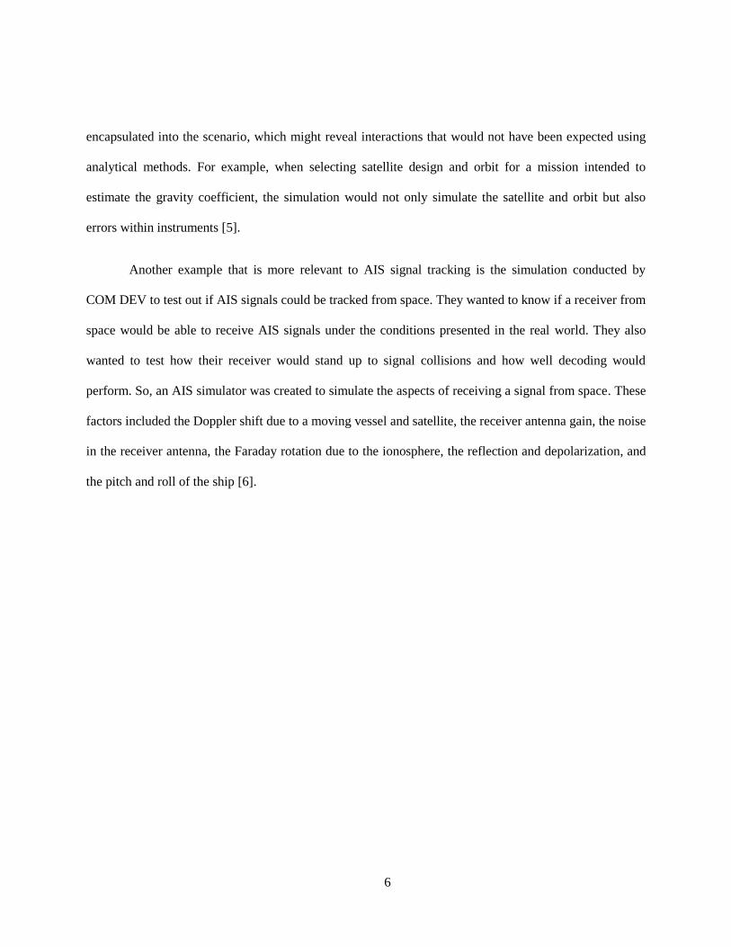
perform. So, an AIS simulator was created to simulate the aspects of receiving a signal from space. These
factors included the Doppler shift due to a moving vessel and satellite, the receiver antenna gain, the noise
in the receiver antenna, the Faraday rotation due to the ionosphere, the reflection and depolarization, and
the pitch and roll of the ship [6].
7
Figure 1: The simulated scenario of AIS signal detection from space [6]
COM DEV Ltd and ORBCOMM Inc. are companies that design and build space equipment and
satellites. Both are perusing larger coverage of AIS signal capture. The simulation algorithm developed,
of one or more satellites tracking a large number of targets, could aid in the design of future AIS missions
such as the number of satellites to use and their characteristics (orbit, inclination etc.). This could be taken
further with multi-disciplinary optimization (MDO) where using one of its multiple techniques, such as a
Genetic Algorithm, along with the simulation algorithm can create a minimal cost plan that meets the
specific mission criteria.
1.3.2 Mission Operations
Once past the initial design of the satellite, preparation for the support system known as the
Mission Operations needs to be considered. Mission Operations are what takes care of all the necessary
8
work that is required once the space mission is launched and working. If there is a satellite or multiple
satellites, they will be creating data that needs to be handled by personnel on the ground. The location of
the ground station and the flow of information needs to be planned so that there are no bottle necks in the
data stream that reaches the client. The simulation would also produce data in order to train personnel in
areas such as how to work in a team. This approach has been proposed to train new teams in handling all
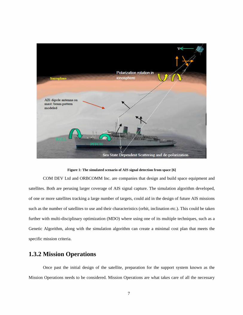
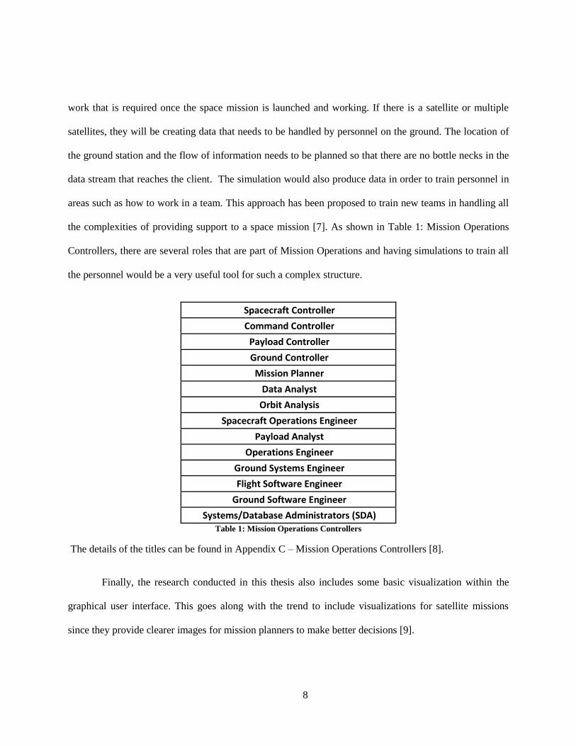
the complexities of providing support to a space mission [7]. As shown in Table 1: Mission Operations
Controllers, there are several roles that are part of Mission Operations and having simulations to train all
the personnel would be a very useful tool for such a complex structure.
Spacecraft Controller
Command Controller
Payload Controller
Ground Controller
Mission Planner
Data Analyst
Orbit Analysis
Spacecraft Operations Engineer
Payload Analyst
Operations Engineer
Ground Systems Engineer
Flight Software Engineer
Ground Software Engineer
Systems/Database Administrators (SDA) Table 1: Mission Operations Controllers
The details of the titles can be found in Appendix C – Mission Operations Controllers [8].
Finally, the research conducted in this thesis also includes some basic visualization within the
graphical user interface. This goes along with the trend to include visualizations for satellite missions
since they provide clearer images for mission planners to make better decisions [9].
9
Simulation in the field of Applied Science is an extremely important part of developing a product
or service to be used in industry, the consumer space, or academia. Many fields of study are covered
when trying to model and simulate a scenario in the real world. These simulations developed have
applications in social, economic, financial, and scientific/engineering domains [10]. Although the
research conducted in this thesis is meant mainly for space applications, such research can have economic
and social implications due to its usefulness in tracking targets such as ships, people, vehicles, etc.
Furthermore, the research can be used to set up mission operation parameters such as personnel and
equipment needed. Thus, it has its place among the many different simulations that are out today.
1.3.3 Growing Needs of Satellite AIS
There is a growing need for governments to keep track of their coastal waters and to monitor
illegal activity. With the limited range of coastal AIS detection stations, the vast majority of the ocean is
left unmonitored. This leaves open the possibility for illegal activity such as fishing in protected areas,
drug trading, and violation of coastal boundaries. The distance at which a shore based AIS station can
detect signals from a ship is 75km [11], with distances between ships being less. The relatively small
distance at which ground-based AIS systems can detect AIS signals from a ship is a hindrance to
maintaining global coverage of ship traffic. Space based systems of AIS detection can get around this
problem.
Currently the two major commercial providers of AIS data are COM DEV and ORBCOMM.
Both of these AIS data providers differ in the number of satellites and configurations of satellites such
their orbits, performance for AIS signal detection, and number of satellites. A client will want to
understand the performance of these providers or a combination of the assets (the asset in this case is data
from a specific satellite) of these providers, a simulation providing a viable way to gauge this. A provider
10
would also want to gauge performance of future configurations that they are planning to put up, in order
to make a better business decision.
1.4 Satellite Geolocation
1.4.1 Location Determination vs. Orbit Determination
The term satellite geolocation is ambiguous and needs to be further clarified so that
material presented later in this research is not misunderstood. Satellite geolocation is a means to find or
locate a satellite in space. This can be further split into two categories of satellite location: determination
of position and satellite orbit determination. The position of the satellite is the instantaneous position that
a satellite is in at a particular time in a given reference frame. Satellite orbit determination is finding the
six Keplerian elements [12] so that the satellite’s position can be found with time being the input into this
system. This would allow the position of the satellite to be propagated in time.
There are several ways to determine the location of the satellite (which will be discussed in
further detail in section 2.2 Satellite Geolocation Methods). Once the location is found, the orbit of the
satellite can be constructed. To construct the orbit of the satellite, six independent points need to be
gathered and the six Keplerian orbital parameters can be constructed [13]. Satellite geolocation in this
research refers to determining the position of the satellite so that the orbit can be determined from these
results.
1.4.2 Satellite Tracking vs. Tracking Satellites
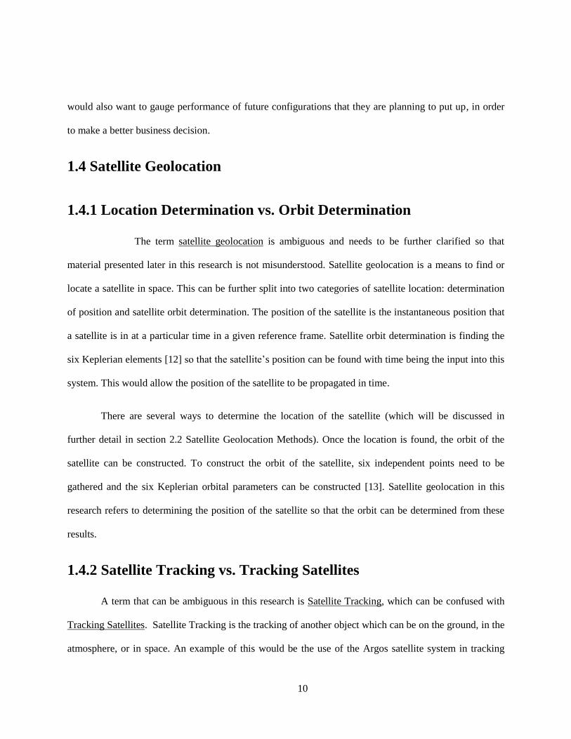
A term that can be ambiguous in this research is Satellite Tracking, which can be confused with
Tracking Satellites. Satellite Tracking is the tracking of another object which can be on the ground, in the
atmosphere, or in space. An example of this would be the use of the Argos satellite system in tracking
11
ground transmitters or the use of Automatic Identification Signal (AIS) equipped satellites to track AIS
signals from ships on the ground.
Figure 2: Satellite Tracking, showing a satellite tracking ground targets
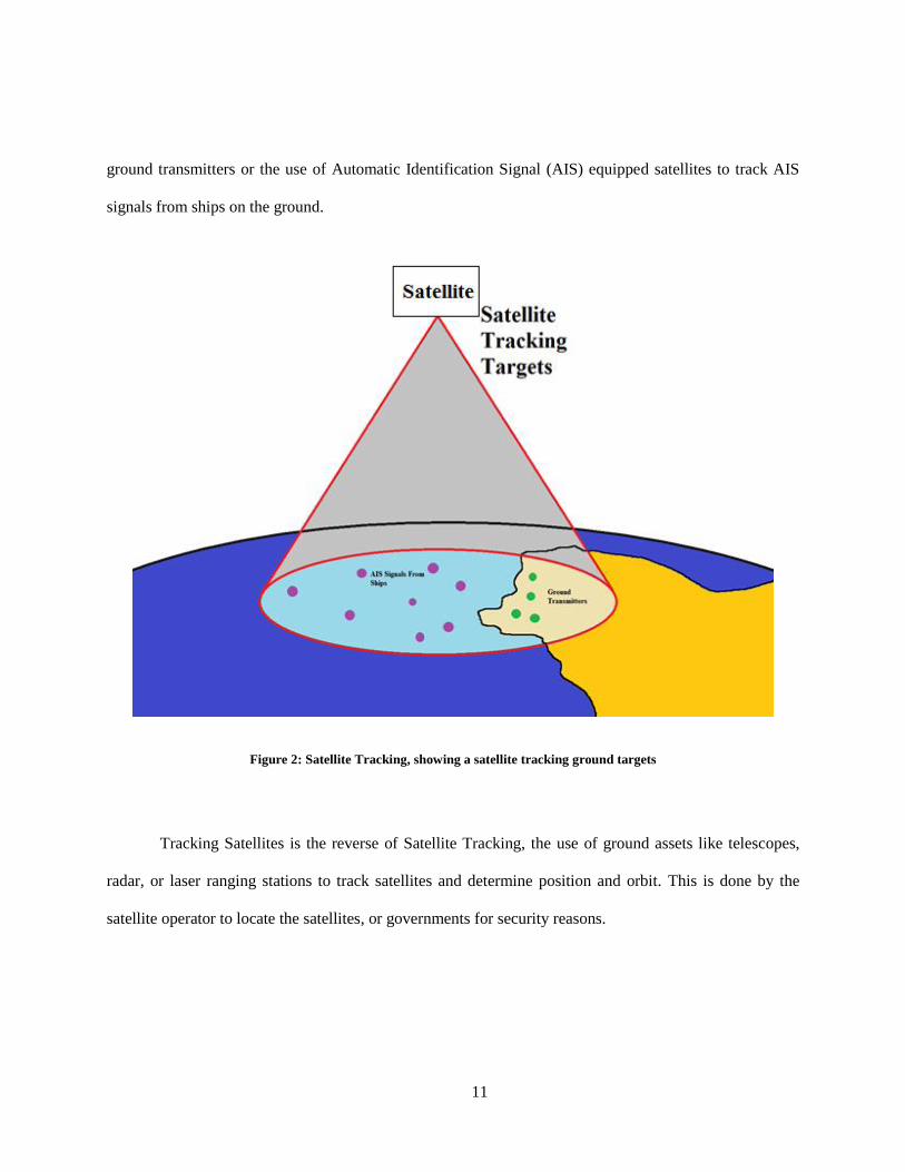
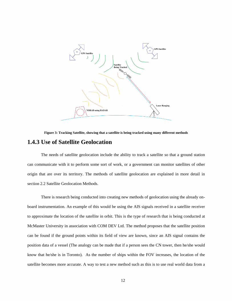
Tracking Satellites is the reverse of Satellite Tracking, the use of ground assets like telescopes,
radar, or laser ranging stations to track satellites and determine position and orbit. This is done by the
satellite operator to locate the satellites, or governments for security reasons.
12
Figure 3: Tracking Satellite, showing that a satellite is being tracked using many different methods
1.4.3 Use of Satellite Geolocation
The needs of satellite geolocation include the ability to track a satellite so that a ground station
can communicate with it to perform some sort of work, or a government can monitor satellites of other
origin that are over its territory. The methods of satellite geolocation are explained in more detail in
section 2.2 Satellite Geolocation Methods.
There is research being conducted into creating new methods of geolocation using the already on-
board instrumentation. An example of this would be using the AIS signals received in a satellite receiver
to approximate the location of the satellite in orbit. This is the type of research that is being conducted at
McMaster University in association with COM DEV Ltd. The method proposes that the satellite position
can be found if the ground points within its field of view are known, since an AIS signal contains the
position data of a vessel (The analogy can be made that if a person sees the CN tower, then he/she would
know that he/she is in Toronto). As the number of ships within the FOV increases, the location of the
satellite becomes more accurate. A way to test a new method such as this is to use real world data from a
13
satellite or to use a simulation. The simulation developed for the research presented in this thesis can be
used to generate such data as which vessels are within the FOV at a particular time, and the probability of
detection included as part of the receiver’s characteristic. It would provide a platform to geolocate the
satellite, which can then be compared with its true location. From there, it can be determined if the
research conducted is valid.
1.5 Thesis Outline
This thesis consists of seven chapters. In this chapter the research subject matter, objectives, and
motivations are all presented. The following chapter will expand on some of the ideas and show how the
objectives of this chapter are fulfilled.
Chapter 2 describes more details on the background material such as Satellite Tracking and
Tracking a Satellite(s). It further delves into the details of AIS and how space based AIS detection is on
the rise.
Chapter 3 introduces the API for the simulation being developed as a continuation of Chapter 1,
explaining why simulations are important. It goes through the detail of what the API can do and the
iterations it has gone through to become the final API that is used to create a tracking simulation at the
current moment. Once the API and the features are explained - details about the more narrow areas
relating to the research are discussed in chapters 4 to 6.
Chapter 4 explains how the attitude used in the simulation is generated, from the inception of the
controller, to developing a satellite model suitable and relevant to the research being conducted, and to
final results that are used in the testing of the simulation (presented in Chapter 6).
Chapter 5 focuses on the ground segment of the simulation and generating the initial data to be
used in testing the simulation.
14
Chapter 6 focuses on the benefits the simulation algorithms provide for the user. Limitations of
the simulation are discussed at the end of the chapter. The chapter also displays how the objectives
presented in Chapter 1 are met. This is achieved by conducting a test simulation and seeing how the
results fair with the objectives laid out in Chapter 1.
Chapter 7 discusses the improvements to be made to the simulation and how the current one
faired compared with the objectives set in Chapter 1.
15
Chapter 2 – Background
2.1 Tracking from a Satellite
Tracking targets from a satellite(s) is used in various applications for military, civilian, and
scientific purposes. The following sections explain and expand on the areas where tracking from space is
conducted. It also explains the use of the simulation algorithm developed in research and how it is
relevant to these areas
2.1.1 Animal Tracking
Animal tracking from space is a technique used by scientists to track animals over a large area
with relatively low cost. Animal tracking started in the early 1970s due to a need to track animals through
long distances and periods to see migration patterns. [14] To track animals on such rough terrain for an
extended period of time would be expensive with other means of tracking. These would include using
aircrafts, which have a high cost of buying time, and using human trackers [15].
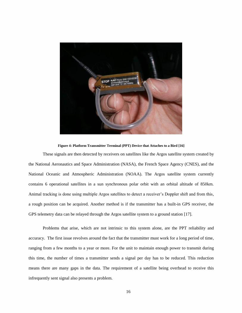
Satellite tracking is done by receiving signals from a Platform Transmitter Terminal (PPT) in the
UHF or VHF band attached to the animal.
16
Figure 4: Platform Transmitter Terminal (PPT) Device that Attaches to a Bird [16]
These signals are then detected by receivers on satellites like the Argos satellite system created by
the National Aeronautics and Space Administration (NASA), the French Space Agency (CNES), and the
National Oceanic and Atmospheric Administration (NOAA). The Argos satellite system currently
contains 6 operational satellites in a sun synchronous polar orbit with an orbital altitude of 850km.
Animal tracking is done using multiple Argos satellites to detect a receiver’s Doppler shift and from this,
a rough position can be acquired. Another method is if the transmitter has a built-in GPS receiver, the
GPS telemetry data can be relayed through the Argos satellite system to a ground station [17].
Problems that arise, which are not intrinsic to this system alone, are the PPT reliability and
accuracy. The first issue revolves around the fact that the transmitter must work for a long period of time,
ranging from a few months to a year or more. For the unit to maintain enough power to transmit during
this time, the number of times a transmitter sends a signal per day has to be reduced. This reduction
means there are many gaps in the data. The requirement of a satellite being overhead to receive this
infrequently sent signal also presents a problem.
17
There is also the issue of the transmitter surviving the environment, along with the problem of the
transmitter moving constantly. The animals that they are attached to could be underwater or in an area
where the signal cannot make it to the satellite (heavy bush, forest, deep valley, etc.) [14]. With all these
factors, the transmitters have to be designed in order to overcome these challenges and one way to do that
is through simulation.
With the target tracking simulation augmented to track PPTs and the addition of focus on
environmental factors such as temperature changes, the effect of precipitation, or PPT position and
orientation changes, a test of the performance of PPT devices can be found. From that, scientists
determine the proper characteristics to give to the PPT. This could include the number of times a message
is sent, the length of transmission time and so on. This would help test the PPT in a situation similar to the
real world without the cost of building and deploying the unit. HAUSAT-2, a 25kg nanosatellite, is being
developed to study the ecology of animals through tracking using Animal Tracking system (ATS) [18],
similar to NTS onboard NTS nanosatellite.
2.1.2 Human Tracking
Another application of satellite tracking is to track people. The UK government was formulating
a plan to use tracking from space to keep track of convicts [19]. The aspects that can be analyzed are the
detection of these transmitters with cellular networks instead of satellites or the merging of a cellular
network with a satellite network to perform an analysis. Currently all non-military tracking of people is
performed using cellular networks [20]. It would be useful for future researchers to have access to a
program which can perform analysis on this system or a merger of systems.
The advantage of using the simulation developed in this research is that a large number of
dynamic targets can be tracked and analysed for patterns. The simulation could also check for coverage or
perform some other statistical analysis on the detected data.
18
2.1.3 Vehicular and Aircraft Traffic
Vehicular traffic and air traffic monitoring is an important part of what governments around the
world do in order to manage and maintain these methods of transportation. Vehicular traffic is monitored
in order to plan out roads and reduce congestion. Aircraft traffic is used to manage passengers and cargo
aircraft traffic to avoid congestion at airports, to ensure safe minimum distances between aircraft, and to
help plan future expansions. This is especially true for the International Civil Aviation Organization
(ICAO), a United Nations organization created in 1944 “to promote the safe and orderly development of
international civil aviation throughout the world” [21].
Since most vehicles do not have transmitters onboard sending out signals with location and
heading, some have proposed to track ground vehicles using radar based remote sensing techniques to
cover wide areas for road traffic monitoring [22]. If some vehicles outfitted with transmitters were
accessed, it would provide vital information about traffic. These kinds of situations have potential to be
explored through simulation using satellites. The ability for a satellite to cover a massive area would give
it a great advantage over terrestrial tracking methods.
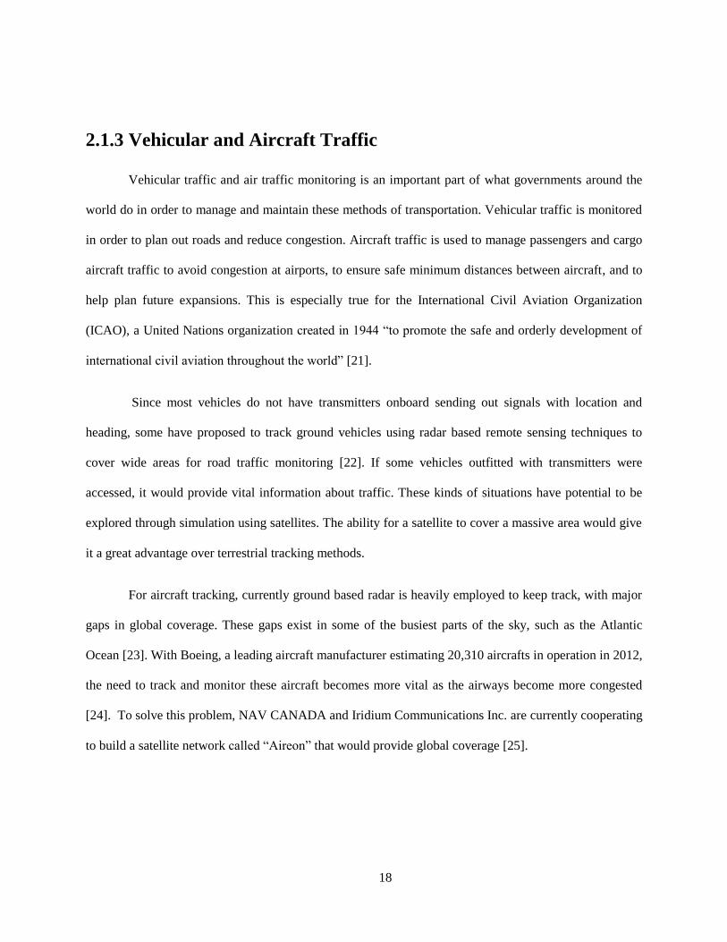
For aircraft tracking, currently ground based radar is heavily employed to keep track, with major
gaps in global coverage. These gaps exist in some of the busiest parts of the sky, such as the Atlantic
Ocean [23]. With Boeing, a leading aircraft manufacturer estimating 20,310 aircrafts in operation in 2012,
the need to track and monitor these aircraft becomes more vital as the airways become more congested
[24]. To solve this problem, NAV CANADA and Iridium Communications Inc. are currently cooperating
to build a satellite network called “Aireon” that would provide global coverage [25].
19
Figure 5: Aireon's Global Coverage Compared with Current Coverage. The orange represents the areas of coverage. [26]
This would be an ideal situation for a simulation to see how much traffic can actually be tracked
and what would be required in terms of number of satellites and the receiver onboard the satellite.
2.1.4 Vessel Tracking
Vessel tracking from space is an emerging area of research and development due to need for
governments and companies to monitor vessel traffic across the world’s waterways. The Automatic
Identification System (AIS) is a communication system designed to provide information to vessels and
offshore stations about the current vessel’s position, identification, course, and speed. This system was
designed to help vessels avoid collisions at sea through continuous monitoring of these signals. Not only
is this system helpful for collision avoidance, but it also assists the coast guard and search and rescue
organizations [27].The AIS system communicates in the VHF-band and was designed to be used with a
maximum distance of 74km for inter-vessel communication. However, space borne AIS signal detection
systems are now already up and running. These systems allow coverage of vessels well beyond the limit
imposed by the horizon on a vessel. A satellite orbiting in Low Earth Orbit (LEO) would have a range to
the horizon of more than 1000 nautical miles (1852km). This allows for a satellite to have a massive field
of view, giving it access to thousands of ships at a given instant. The main reason for the move into space
20
was to track a massive number of vessels over time for use in monitoring for government and non-
governmental agencies [11].
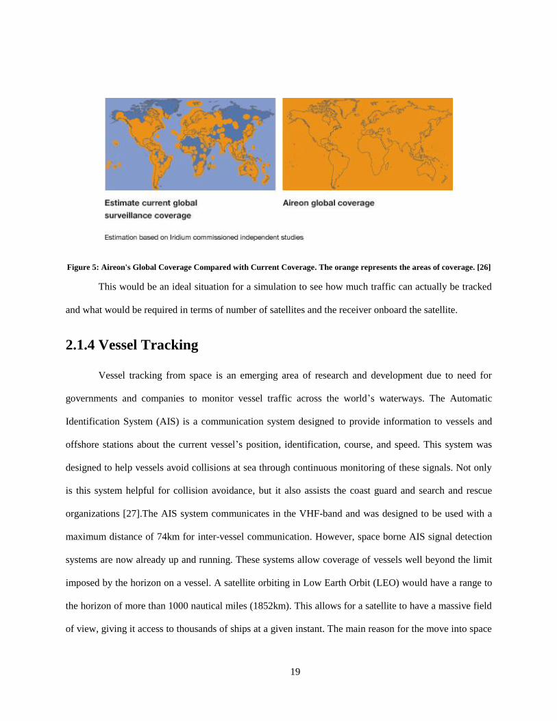
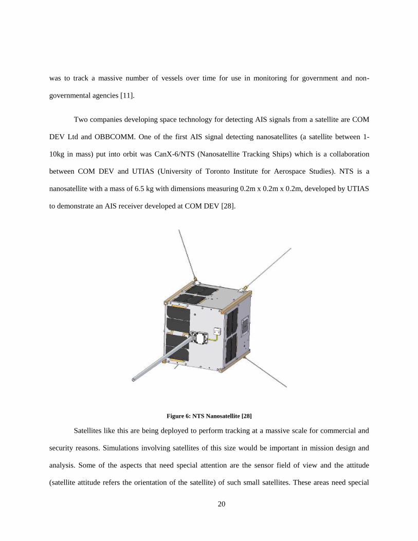
Two companies developing space technology for detecting AIS signals from a satellite are COM
DEV Ltd and OBBCOMM. One of the first AIS signal detecting nanosatellites (a satellite between 1-
10kg in mass) put into orbit was CanX-6/NTS (Nanosatellite Tracking Ships) which is a collaboration
between COM DEV and UTIAS (University of Toronto Institute for Aerospace Studies). NTS is a
nanosatellite with a mass of 6.5 kg with dimensions measuring 0.2m x 0.2m x 0.2m, developed by UTIAS
to demonstrate an AIS receiver developed at COM DEV [28].
Figure 6: NTS Nanosatellite [28]
Satellites like this are being deployed to perform tracking at a massive scale for commercial and
security reasons. Simulations involving satellites of this size would be important in mission design and
analysis. Some of the aspects that need special attention are the sensor field of view and the attitude
(satellite attitude refers the orientation of the satellite) of such small satellites. These areas need special
21
attention because of lower power availability to small satellites and the fact that small satellites are more
susceptible to perturbations, causing drastic change in attitude.
2.2 Satellite Geolocation Methods
The location of a satellite can be found using several methods and one of the newer proposed
methods (mentioned in 1.3 Applications of Satellite Target Tracking Simulation) uses targets detected in
the satellite FOV to approximate the location of the satellite. In the case of a satellite tracking ships using
AIS signals, the satellite would be able to approximate its location by seeing which ships are within its
field of view. The great advantage to this method is that the satellite can use its main payload, the AIS
receiver, to locate its general position over the Earth. The older methods of satellite geolocation that are
still used today and the methods/tools are as follows.
2.2.1 Satellite Laser Ranging
Satellite Laser Ranging (SLR) is a technique of measuring the distance to a satellite from a
ground station by reflecting ultra-short pulses of light. It measures the round-trip time for the light to
reflect off the satellite to measure the distance. The satellites which can be tracked like this have retro
reflectors attached for the light to bounce back from. SLR is currently the most accurate technique of
determining geocentric position of an Earth satellite. SLR was first used by NASA in 1964 with the
launch of the Beacon-B satellite, which had meter accuracies. Now that number has shrunk to millimetre
accuracies. A global community of SLR was formed and is called The International Laser Ranging
Service [29].
2.2.2 Radar
One other major technique used to track satellites is using radar. This method is most prominently
used by NORAD which has the Precision Avionics Vectoring Equipment Phased Array Warning System
22
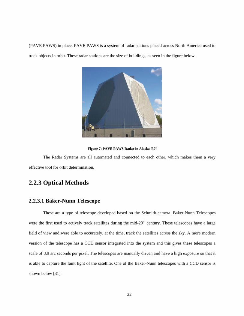
(PAVE PAWS) in place. PAVE PAWS is a system of radar stations placed across North America used to
track objects in orbit. These radar stations are the size of buildings, as seen in the figure below.
Figure 7: PAVE PAWS Radar in Alaska [30]
The Radar Systems are all automated and connected to each other, which makes them a very
effective tool for orbit determination.
2.2.3 Optical Methods
2.2.3.1 Baker-Nunn Telescope
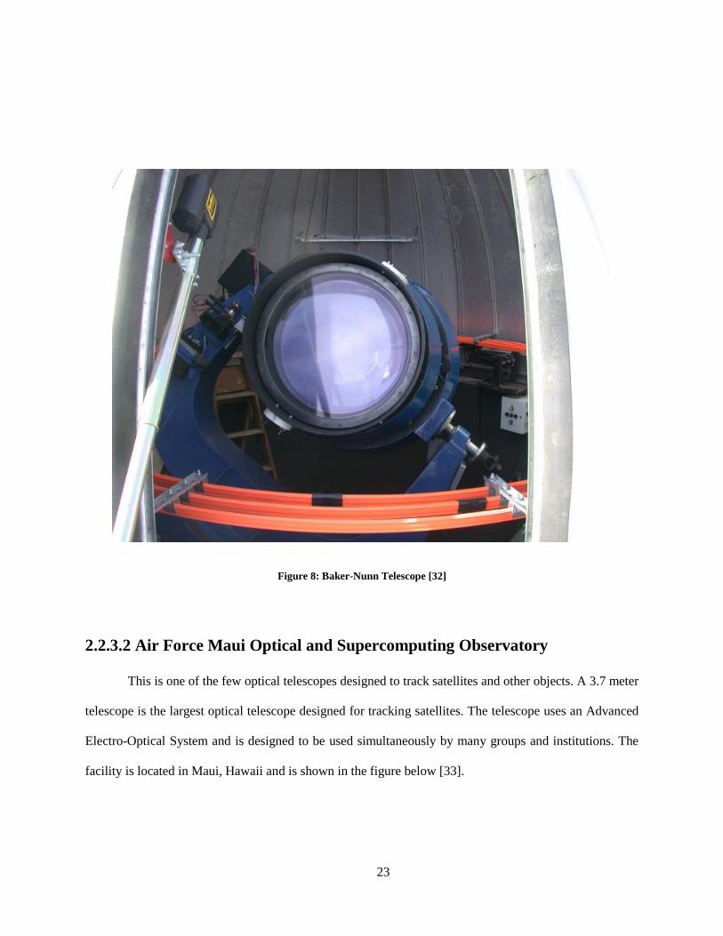
These are a type of telescope developed based on the Schmidt camera. Baker-Nunn Telescopes
were the first used to actively track satellites during the mid-20th century. These telescopes have a large
field of view and were able to accurately, at the time, track the satellites across the sky. A more modern
version of the telescope has a CCD sensor integrated into the system and this gives these telescopes a
scale of 3.9 arc seconds per pixel. The telescopes are manually driven and have a high exposure so that it
is able to capture the faint light of the satellite. One of the Baker-Nunn telescopes with a CCD sensor is
shown below [31].
23
Figure 8: Baker-Nunn Telescope [32]
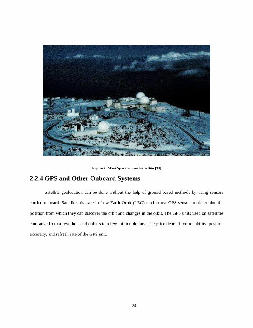
2.2.3.2 Air Force Maui Optical and Supercomputing Observatory
This is one of the few optical telescopes designed to track satellites and other objects. A 3.7 meter
telescope is the largest optical telescope designed for tracking satellites. The telescope uses an Advanced
Electro-Optical System and is designed to be used simultaneously by many groups and institutions. The
facility is located in Maui, Hawaii and is shown in the figure below [33].
24
Figure 9: Maui Space Surveillance Site [33]
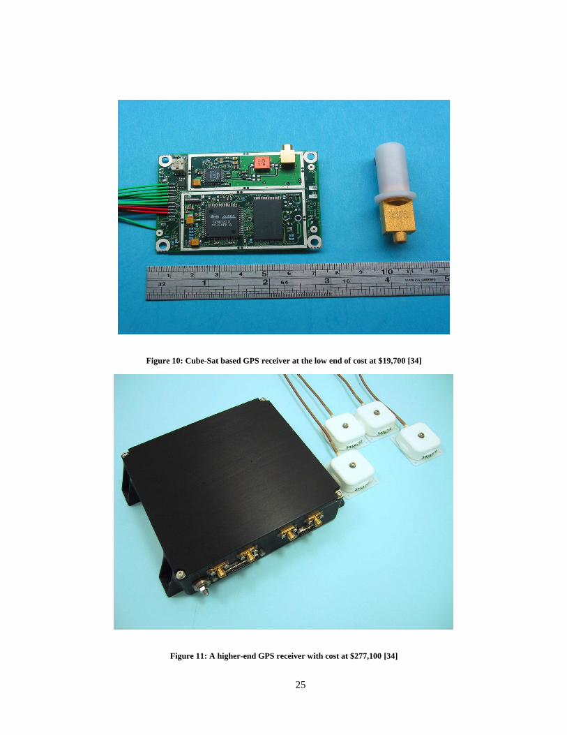
2.2.4 GPS and Other Onboard Systems
Satellite geolocation can be done without the help of ground based methods by using sensors
carried onboard. Satellites that are in Low Earth Orbit (LEO) tend to use GPS sensors to determine the
position from which they can discover the orbit and changes in the orbit. The GPS units used on satellites
can range from a few thousand dollars to a few million dollars. The price depends on reliability, position
accuracy, and refresh rate of the GPS unit.
25
Figure 10: Cube-Sat based GPS receiver at the low end of cost at $19,700 [34]
Figure 11: A higher-end GPS receiver with cost at $277,100 [34]
26
The use of a GPS receiver is not possible for higher orbits due to the 20,000 km altitude of the
GPS constellation. Therefore, the use of GPS receivers is limited to LEO orbits. The GPS receivers
themselves can draw a substantial amount of power, especially for smaller satellites. The receiver shown
in Figure 10: Cube-Sat based GPS receiver at the low end of cost at $19,700 , is made for Cube-Sats and
draws 1 Watt of power, substantial for nanosatellites.
Another onboard method of detecting the location of the satellite is using a 3-axis magnetometer
to detect the Earth’s magnetic field. The Earth’s magnetic field is not uniform. Using this fact, the
magnetic field can be used to determine the location of the satellite [35]. Once a few location points are
known, the satellite’s orbit can be determined.
2.3 Satellite Automatic Identification System (AIS) Detection
2.3.1 History and Function of the Automatic Identification System
(AIS)
The Automatic Identification System standard was formally adopted in 1998 by the International
Maritime Organization (IMO). The International Maritime Organization is a United Nations agency
which describes itself as an “agency with responsibility for the safety and security of shipping and
the prevention of marine pollution by ships” [36]. This agency was set up in order to set a standard for
any vessel at sea, most importantly in improving safety at sea since 90 percent of global trade is done
through shipping. In 1948 the United Nations set up the IMO to handle set guidelines for any maritime
activity [36]. The scope of the AIS system is put as follows from the IMO:
“1.2 The AIS should improve the safety of navigation by assisting in the efficient navigation of ships, protection of the environment, and operation of Vessel Traffic Services (VTS), by satisfying the following functional requirements: .1 in a ship-to-ship mode for collision avoidance; .2 as a
27
means for littoral States to obtain information about a ship and its cargo; and .3 as a VTS tool, i.e. ship-to-shore (traffic management). 1.3 The AIS should be capable of providing to ships and to competent authorities, information from the ship, automatically and with the required accuracy and frequency, to facilitate accurate tracking. Transmission of the data should be with the minimum involvement of ship's personnel and with a high level of availability [37].”
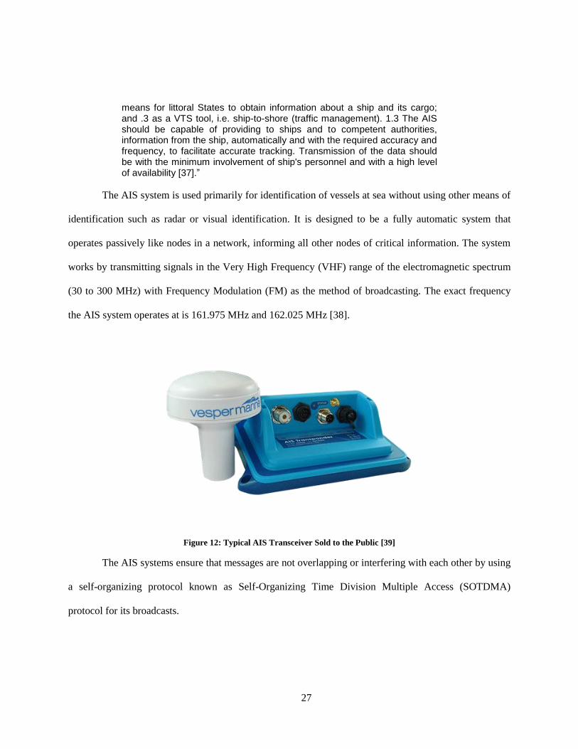
The AIS system is used primarily for identification of vessels at sea without using other means of
identification such as radar or visual identification. It is designed to be a fully automatic system that
operates passively like nodes in a network, informing all other nodes of critical information. The system
works by transmitting signals in the Very High Frequency (VHF) range of the electromagnetic spectrum
(30 to 300 MHz) with Frequency Modulation (FM) as the method of broadcasting. The exact frequency
the AIS system operates at is 161.975 MHz and 162.025 MHz [38].
Figure 12: Typical AIS Transceiver Sold to the Public [39]
The AIS systems ensure that messages are not overlapping or interfering with each other by using
a self-organizing protocol known as Self-Organizing Time Division Multiple Access (SOTDMA)
protocol for its broadcasts.
28
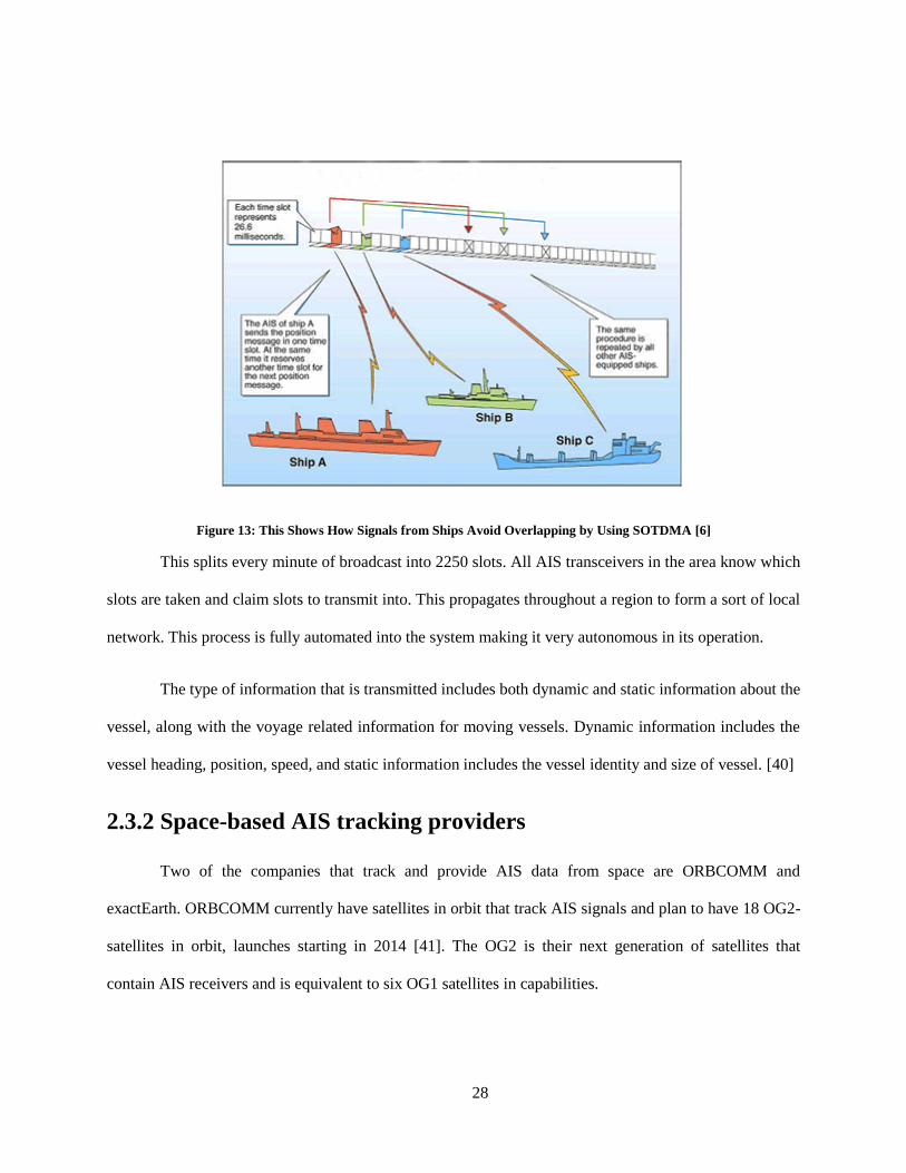
Figure 13: This Shows How Signals from Ships Avoid Overlapping by Using SOTDMA [6]
This splits every minute of broadcast into 2250 slots. All AIS transceivers in the area know which
slots are taken and claim slots to transmit into. This propagates throughout a region to form a sort of local
network. This process is fully automated into the system making it very autonomous in its operation.
The type of information that is transmitted includes both dynamic and static information about the
vessel, along with the voyage related information for moving vessels. Dynamic information includes the
vessel heading, position, speed, and static information includes the vessel identity and size of vessel. [40]
2.3.2 Space-based AIS tracking providers
Two of the companies that track and provide AIS data from space are ORBCOMM and
exactEarth. ORBCOMM currently have satellites in orbit that track AIS signals and plan to have 18 OG2-
satellites in orbit, launches starting in 2014 [41]. The OG2 is their next generation of satellites that
contain AIS receivers and is equivalent to six OG1 satellites in capabilities.
29
exactEarth® is a company owned by COM DEV International Ltd. and HISDESAT, which is
created to provide global coverage of AIS data to clients around the world. exactEarth® has created the
exactView™, which is a data service that contains both satellite and ground assets that track AIS signals,
the first satellite used is NTS, with three other satellites already in orbit and seven others to put into
service from 2014-2018 [42].
2.4 Coordinate Systems
The coordinate systems used in the simulation include the Earth Centered Earth-Fixed (ECEF)
and the World Geodetic System 1984 (WGS 84). The ECEF system represents a Cartesian coordinate
system which has the origin located at the center of mass of Earth, with the X-axis pointing Prime
Meridian and the Z-axis goes through the North Pole, with the Y-axis forming a right-handed system. As
the name implies the ECEF system is fixed to the Earth, therefore it has the effects of nutation, procession
and Earth’s wobble. To represent the Earth, the WGS 84 ellipsoid is used. The WGS 84 is a standard
geodetic reference system created to represent the Earth shape of the Earth and is extensively used in
mapping. One of the big uses of the WGS 84 is for the Global Positioning System.
To generate the satellite path for the satellite(s) in the simulation, the SGP4 propagator is used.
The SGP4 is the last of the Simplified General Perturbations (SGP) model series and was created by the
United States Air Force to propagate the satellite positions. This model can be used with the Two-Line
Element file format create by NORAD. Development began in the 1960s with the final version available
on the internet being released in 1996-1997. The coordinate system used to represent the SGP4 position
and its derivatives are in the TEME coordinate frame [43]. Since there is no official definition of TEME,
a good resource to find out details is Fundamentals of Astrodynamics and Applications by David A.
Vallado.
30
Chapter 3 – Development of Application
Programming Interface for the Simulation
3.1 Commercial/ Open Source APIs and Simulation
Orekit is an open source dynamics library written in Java with low level functions to be used in
any application written by a client. Orekit has the ability to generate orbits using many different
propagators, including two-line orbits all the way to the SGP4 propagator. It contains a variety of gravity
models with the models of different representations of the Earth ellipsoid. There are some attitude models
for spacecraft, but no ability to generate attitude based on the physical dimensions of the satellite. It also
has plugins to allow file-based storage or database connectivity [44].
General Mission Analysis Tool is a mission analysis tool that was developed by NASA, public
users, and private space industry partners. It is an open source platform designed to do dynamics and
environment modelling, generate plots and reports, and help in optimizing space missions. There are
propagation models, gravity models, models of celestial bodies, propulsion modelling, and 3D rendering
of the mission. It also provides a GUI with the ability to write quick scripts based on MATLAB syntax
[45].
Both these dynamics libraries have very similar features and are both open-source, making them a
great option for users looking for a free solution. The feature that keeps STK Components above these
two other tools is the ability to create a 3D field of view (FOV) which can detect points within this
polyhedron. With this ability, custom simulation can be made of a FOV tracking moving targets.
31
3.2 Application Programming Interface (API) Models
Over the course of the research, three different API models have been created. The latter two API
versions differ from the first version not only due to feature changes, but also due to change in
programming language. The first API was created using MATLAB and as development continued and
more functionality was required, the STK Components API was integrated using the MATLAB.NET
interface. Once this interface became more of a burden than benefit to the overall API, development of
the second API was started and all code was written with Java™
using STK Components. This allowed for
better integration of STK Components and the use of Java drivers such as JDBC for databases and the
driver for MongoDB. One fact to note is that the API can be thought of as a collection of functions –
written in computer code and with a high level of order – created for a programmer to produce a more
complex algorithm to perform a computation such as the simulation that is made in this research.
3.2.1 Spherical Earth and Circular Orbit API
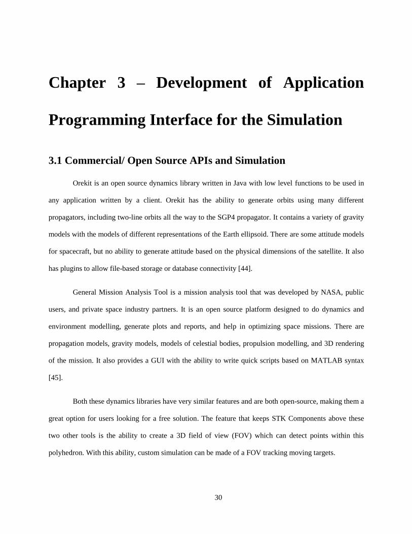
The first API created can be referred to as the spherical API. It is created to perform the most
basic simulation with a single satellite orbiting Earth in a circular orbit. The model used for the Earth was
spherical with a radius of 6378.1km. The field of view (FOV) modeled is circular and to detect any
targets within it, the algorithm used angular distances originating at the center of the Earth. It is seen from
Figure 14: Interior Angle α Corresponding to FOV Angle θ the FOV angle θ corresponds to an interior
angle α. This is how the algorithm initially detected targets on the Earth’s surface.
32
Figure 14: Interior Angle α Corresponding to FOV Angle θ
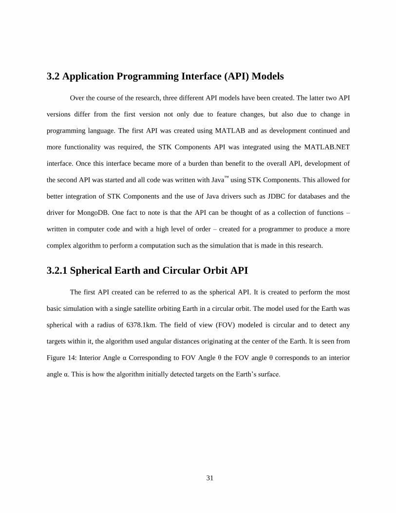
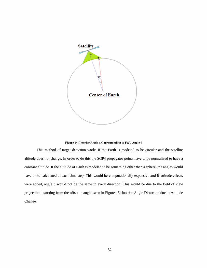
This method of target detection works if the Earth is modeled to be circular and the satellite
altitude does not change. In order to do this the SGP4 propagator points have to be normalized to have a
constant altitude. If the altitude of Earth is modeled to be something other than a sphere, the angles would
have to be calculated at each time step. This would be computationally expensive and if attitude effects
were added, angle α would not be the same in every direction. This would be due to the field of view
projection distorting from the offset in angle, seen in Figure 15: Interior Angle Distortion due to Attitude
Change.
33
Figure 15: Interior Angle Distortion due to Attitude Change
This version of the API did not allow for many complexities in the simulation with many of the
variable mission (such as changing attitude, non-circular orbit, and ellipsoid representation of Earth), but
did allow a quick simulation to be performed with little programming and smaller computation time.
3.2.1.1 Field Of View Update
One of the problems with the spherical API version is the inability to change the FOV shape,
circular orbit, and spherical Earth. In order to deal with changing attitude, changing altitude, a non-
spherical Earth, and a FOV that is not circular, STK Components was integrated into MATLAB using the
MATLAB.NET interface. What this interface allowed was to use some of the API of STK Components,
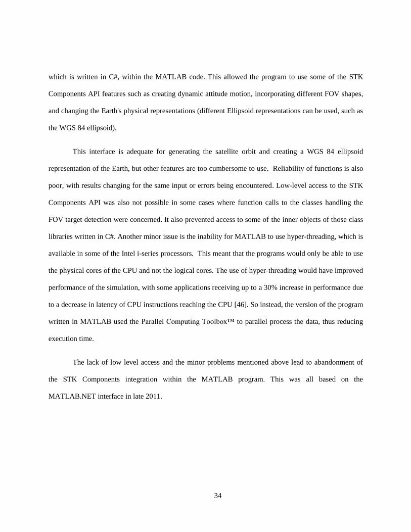
34
which is written in C#, within the MATLAB code. This allowed the program to use some of the STK
Components API features such as creating dynamic attitude motion, incorporating different FOV shapes,
and changing the Earth's physical representations (different Ellipsoid representations can be used, such as
the WGS 84 ellipsoid).
This interface is adequate for generating the satellite orbit and creating a WGS 84 ellipsoid
representation of the Earth, but other features are too cumbersome to use. Reliability of functions is also
poor, with results changing for the same input or errors being encountered. Low-level access to the STK
Components API was also not possible in some cases where function calls to the classes handling the
FOV target detection were concerned. It also prevented access to some of the inner objects of those class
libraries written in C#. Another minor issue is the inability for MATLAB to use hyper-threading, which is
available in some of the Intel i-series processors. This meant that the programs would only be able to use
the physical cores of the CPU and not the logical cores. The use of hyper-threading would have improved
performance of the simulation, with some applications receiving up to a 30% increase in performance due
to a decrease in latency of CPU instructions reaching the CPU [46]. So instead, the version of the program
written in MATLAB used the Parallel Computing Toolbox™ to parallel process the data, thus reducing
execution time.
The lack of low level access and the minor problems mentioned above lead to abandonment of
the STK Components integration within the MATLAB program. This was all based on the
MATLAB.NET interface in late 2011.
35
3.2.2 Single Satellite Non-Spherical Earth and Non-Circular Orbit
API
The second version of the API is when the switch to the Java programming language with STK
Components was used. The earlier API was riddled with bugs due to the use of the MATLAB.NET
interface and the code was difficult to use due to the long time it takes to modify code. The simulation
created with the previous API is also very primitive due to many of the simplifications such as the circular
Earth, a circular orbit, and lack of attitude motion. The other major problem with the spherical API that
had the integration with STK Components is the lack of access to the lower level functions.
The need for simplicity and access to lower levels of the simulation (such as the ability to have
direct access to calculation that occurs at every time-step) led to the development of a modular API that
would allow the research objectives to be met. The API is split into three sections: the satellite model, the
target model, and the data model.
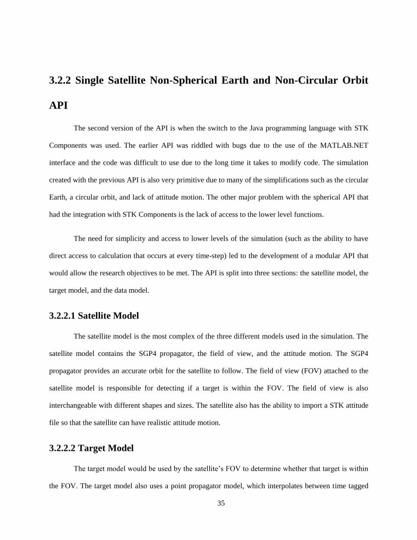
3.2.2.1 Satellite Model
The satellite model is the most complex of the three different models used in the simulation. The
satellite model contains the SGP4 propagator, the field of view, and the attitude motion. The SGP4
propagator provides an accurate orbit for the satellite to follow. The field of view (FOV) attached to the
satellite model is responsible for detecting if a target is within the FOV. The field of view is also
interchangeable with different shapes and sizes. The satellite also has the ability to import a STK attitude
file so that the satellite can have realistic attitude motion.
3.2.2.2 Target Model
The target model would be used by the satellite’s FOV to determine whether that target is within
the FOV. The target model also uses a point propagator model, which interpolates between time tagged
36
locations provided for a specific type of target. A transmitter is also included to check if the target is
transmitting a position signal; the signal is used to determine if the satellite detects this target as the
simulation is underway. The transmitting period changes depending on the type of vessel that is specified
and to make sure that all vessels of the same type do not transmit at the same time step. The transmitting
period is shifted by a random number.
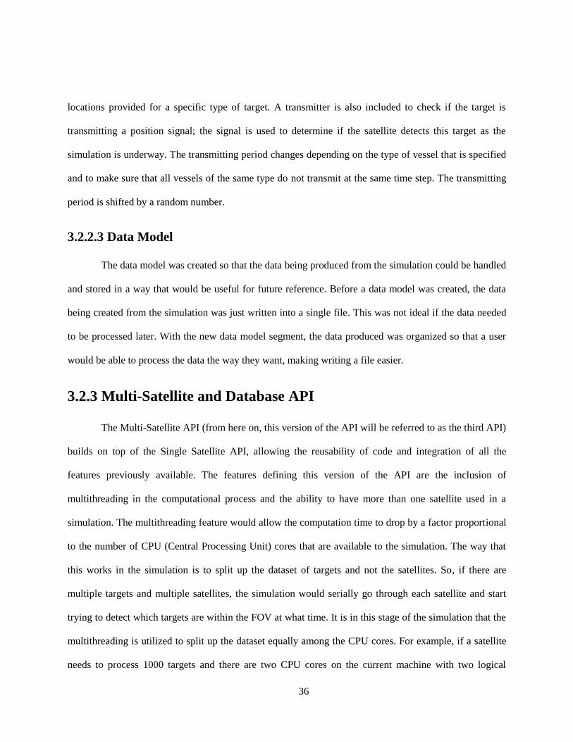
3.2.2.3 Data Model
The data model was created so that the data being produced from the simulation could be handled
and stored in a way that would be useful for future reference. Before a data model was created, the data
being created from the simulation was just written into a single file. This was not ideal if the data needed
to be processed later. With the new data model segment, the data produced was organized so that a user
would be able to process the data the way they want, making writing a file easier.
3.2.3 Multi-Satellite and Database API
The Multi-Satellite API (from here on, this version of the API will be referred to as the third API)
builds on top of the Single Satellite API, allowing the reusability of code and integration of all the
features previously available. The features defining this version of the API are the inclusion of
multithreading in the computational process and the ability to have more than one satellite used in a
simulation. The multithreading feature would allow the computation time to drop by a factor proportional
to the number of CPU (Central Processing Unit) cores that are available to the simulation. The way that
this works in the simulation is to split up the dataset of targets and not the satellites. So, if there are
multiple targets and multiple satellites, the simulation would serially go through each satellite and start
trying to detect which targets are within the FOV at what time. It is in this stage of the simulation that the
multithreading is utilized to split up the dataset equally among the CPU cores. For example, if a satellite
needs to process 1000 targets and there are two CPU cores on the current machine with two logical
37
threads, this scenario can be split up into two groups of 500 targets. Once all targets are processed, the
detected ships from each group can be merged.
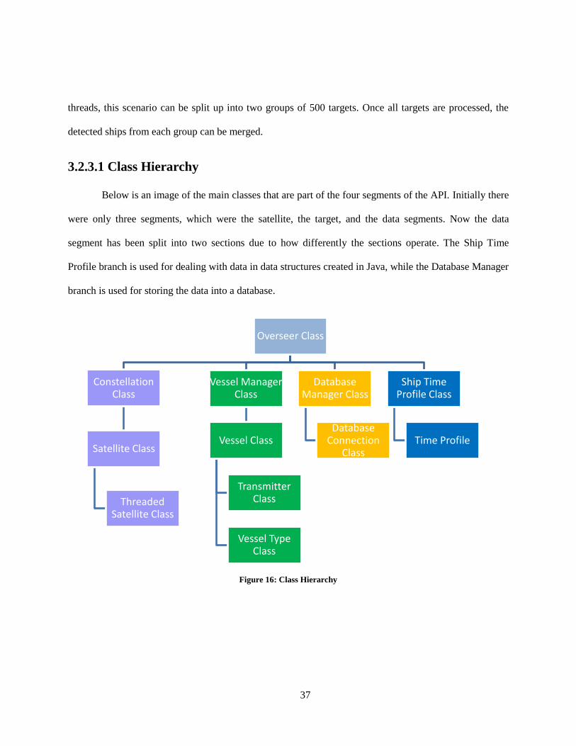
3.2.3.1 Class Hierarchy
Below is an image of the main classes that are part of the four segments of the API. Initially there
were only three segments, which were the satellite, the target, and the data segments. Now the data
segment has been split into two sections due to how differently the sections operate. The Ship Time
Profile branch is used for dealing with data in data structures created in Java, while the Database Manager
branch is used for storing the data into a database.
Figure 16: Class Hierarchy
Overseer Class
Constellation Class
Satellite Class
Threaded Satellite Class
Vessel Manager Class
Vessel Class
Transmitter Class
Vessel Type Class
Database Manager Class
Database Connection
Class
Ship Time Profile Class
Time Profile
38
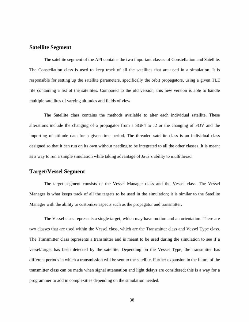
Satellite Segment
The satellite segment of the API contains the two important classes of Constellation and Satellite.
The Constellation class is used to keep track of all the satellites that are used in a simulation. It is
responsible for setting up the satellite parameters, specifically the orbit propagators, using a given TLE
file containing a list of the satellites. Compared to the old version, this new version is able to handle
multiple satellites of varying altitudes and fields of view.
The Satellite class contains the methods available to alter each individual satellite. These
alterations include the changing of a propagator from a SGP4 to J2 or the changing of FOV and the
importing of attitude data for a given time period. The threaded satellite class is an individual class
designed so that it can run on its own without needing to be integrated to all the other classes. It is meant
as a way to run a simple simulation while taking advantage of Java’s ability to multithread.
Target/Vessel Segment
The target segment consists of the Vessel Manager class and the Vessel class. The Vessel
Manager is what keeps track of all the targets to be used in the simulation; it is similar to the Satellite
Manager with the ability to customize aspects such as the propagator and transmitter.
The Vessel class represents a single target, which may have motion and an orientation. There are
two classes that are used within the Vessel class, which are the Transmitter class and Vessel Type class.
The Transmitter class represents a transmitter and is meant to be used during the simulation to see if a
vessel/target has been detected by the satellite. Depending on the Vessel Type, the transmitter has
different periods in which a transmission will be sent to the satellite. Further expansion in the future of the
transmitter class can be made when signal attenuation and light delays are considered; this is a way for a
programmer to add in complexities depending on the simulation needed.
39
Database Segment and Ship Time Profile
These segments are used to store all the data that is generated when a simulation is performed.
The Database Manager and Database Connection class follow the same pattern as the other two segments.
The Database Manager keeps track of multiple connections to Database Connections, which are
connections to databases such as Oracle, MySQL or Microsoft Access. The database connections are to
be used when the simulation produces more data than the system RAM will allow.
If the simulation is small enough the data can be stored on the Random Access Memory (RAM)
by using the class’s Ship Time Profile, a data-structure that holds the targets that were detected by the
satellite(s) at a certain time. This also allows another avenue for a programmer to create a simulation in
which the data on the RAM can be written to the Hard Drive Disk (HDD) in file format.
MongoDB
For the simulation tests conducted in 6.3 Test, the type of database used is MongoDB. It is what
is known as a NoSQL database. This means the database does not use SQL queries and does not contain
database tables like conventional rational databases. Instead, all values are stored as key-value pairs. The
values in the key-value pair can also be key-value pairs, resulting in a language that is similar to JSON
document formatting. The use of MongoDB is due to it being free and the Java driver being easy to use.
40
Chapter 4 – Satellite Attitude Control
4.1 Satellite Attitude Determination and Attitude Control
Attitude determination and control subsystem (ADCS) is one of the most important functions of a
satellite. The word attitude in the spacecraft context is synonymous with orientation. The ability for a
satellite to orient itself to do something useful is of utmost importance; otherwise a satellite tumbling or
pointing at a random part of space is not of much use. Satellite missions might range from capturing
images of objects, to remote sensing (observing the Earth for scientific purposes), to being able to point
towards a transmitter/receiver located either on Earth or another part of space. With all that said it is very
important that in a simulation with orbiting satellites tracking targets, that the attitude be modelled. The
focus is more on the pointing accuracy than the actual attitude motion itself. In order to do this a
controller for the satellite has to be created to respond to the disturbances that the satellites will encounter
in orbit.
The first step towards controlling the satellites attitude is to measure and estimate the orientation.
This is achieved by using a combination of sensors and points of reference. These points of reference start
with the most basic one, which is the Earth. Then we have the Sun and the Moon, followed by distant
celestial objects and other spacecraft. The celestial objects include stars, nebulas, and quasars which tend
to be the brightest. The latter is the most reliable in terms of precision and accuracy. The reason for this is
quasars tend to billions of light years away and are extremely luminous [47], which means that in practice
they are used as stationary points since any movement at such a distance is almost unnoticeable over a
short period of time. The International Celestial Reference System (TCRS) is an example of a reference
frame which uses quasars as a reference point, specifically 3C 273 as a main source [43]. Coordinate
systems are discussed in more detail in 2.4 Coordinate Systems. For a satellite to have a fully functioning
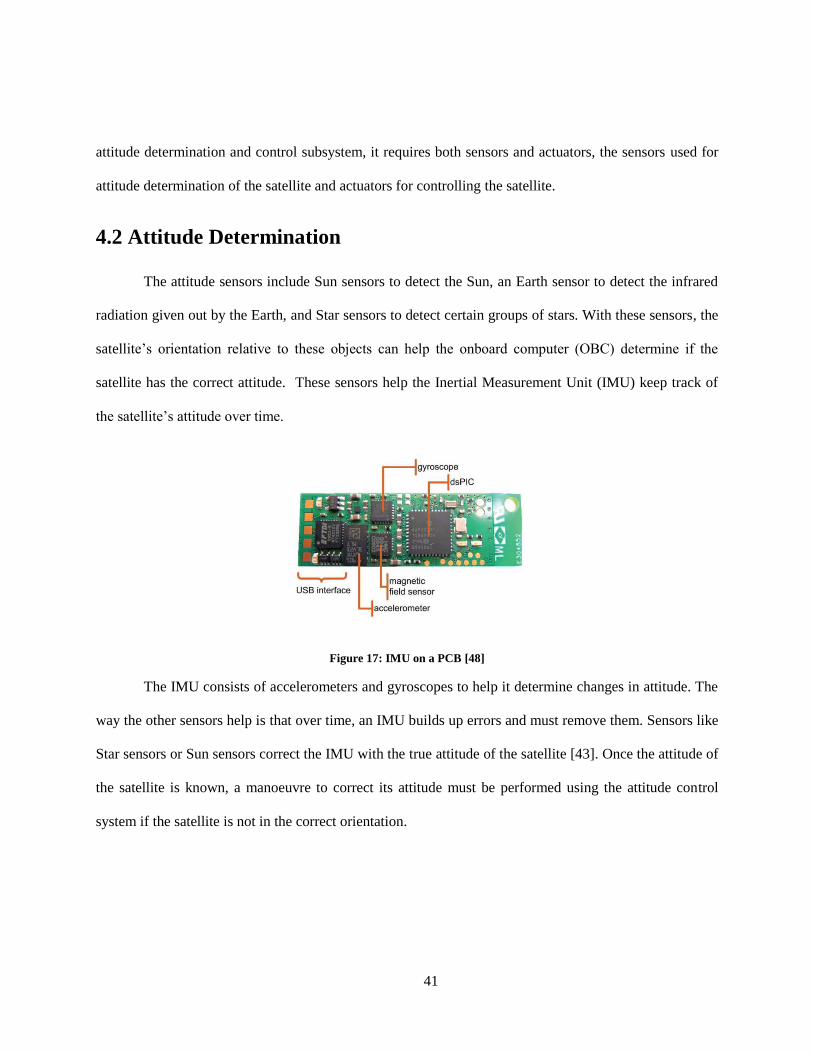
41
attitude determination and control subsystem, it requires both sensors and actuators, the sensors used for
attitude determination of the satellite and actuators for controlling the satellite.
4.2 Attitude Determination
The attitude sensors include Sun sensors to detect the Sun, an Earth sensor to detect the infrared
radiation given out by the Earth, and Star sensors to detect certain groups of stars. With these sensors, the
satellite’s orientation relative to these objects can help the onboard computer (OBC) determine if the
satellite has the correct attitude. These sensors help the Inertial Measurement Unit (IMU) keep track of
the satellite’s attitude over time.
Figure 17: IMU on a PCB [48]
The IMU consists of accelerometers and gyroscopes to help it determine changes in attitude. The
way the other sensors help is that over time, an IMU builds up errors and must remove them. Sensors like
Star sensors or Sun sensors correct the IMU with the true attitude of the satellite [43]. Once the attitude of
the satellite is known, a manoeuvre to correct its attitude must be performed using the attitude control
system if the satellite is not in the correct orientation.
42
4.3 Attitude Control
The attitude control system is the other half of the attitude determination and control subsystem
(ADCS). The control system can either be passive or active, in relation to this research only an active
system is of concern. For an active control system - actuators are needed to apply a torque to the satellite
in order to make it move to the desired attitude.
4.4 Satellite Model
For the purposes of testing that is done in Chapter 6 – Simulation API Features and Test Results,
a model of a nanosatellite has to be created in order to generate a pointing accuracy of about 5 degrees.
This would provide an approximation of the pointing performance of current nanosatellites. For a
baseline, a nanosatellite with the physical characteristics of NTS mentioned in Chapter 1 – Introduction is
modeled with a 6.5kg mass and dimensions measuring 0.2m x 0.2m x 0.2m. The simulation would have
the satellite pointing its AIS receiver in the nadir direction (with a pointing accuracy of approximately 5
degrees), which is the vector perpendicular to the Earth’s surface. In order to have the satellite’s receiver
always pointing towards the Earth, the satellite must have a control system in place to mitigate external
torques applied to the satellite. The model created in this chapter is applied to all the satellites used to test
the simulation algorithm in Chapter 6 – Simulation API Features and Test Results
4.4.1 External Torques
As a satellite is in orbit, it can experience external torques that cause the attitude to drift from a
desired position. Depending on the type of spacecraft and the location of operation, these torques will be
different in term of their source and intensity. For this research, the types of spacecraft being discussed
are nanosatellites and they would be in LEO (Low Earth Orbit, 100 km – 800 km in altitude) [43].
43
The torques the satellite experiences are as follows. First, there is the torque applied to the
satellite structure due to the variation in Earth’s gravitational field. Satellites have varying structure such
as solar panels, instruments, and other parts that are part of the many subsystems onboard the satellites.
Different parts of this structure will experience different gravitational pulls because the Earth’s gravity is
not uniform, leading to torques being applied to the satellite. This force is more apparent in larger and
non-uniform spacecraft, where as in the case of a symmetric spacecraft like the one that is being used in
this research. The gravitational torque would have negligible effect due to the uniformity of the satellite.
This assumption is made in order to simplify the simulation.
Second, there is the aerodynamic drag that is imposed on satellite in a LEO orbit. This is because
the Earth’s atmosphere does not completely end at 100 km in altitude. This is not a problem for satellites
in higher obits but is a concern for satellites in LEO. Third, there is magnetic torque applied on the
satellite. This is caused by the Earth’s magnetic field and its interaction with the metal frame and the
internal electronics of the satellite. The magnetic field is not uniform and the satellite’s position is
changing, moving relative to a magnetic field vector, causing the magnetic moment on the satellite to
change over time. This is especially true at the magnetic North and South poles where the magnetic field
direction changes by 90 degrees compared to the field direction at the equator.
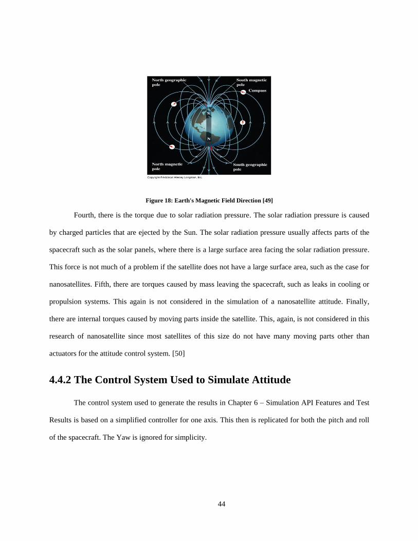
44
Figure 18: Earth's Magnetic Field Direction [49]
Fourth, there is the torque due to solar radiation pressure. The solar radiation pressure is caused
by charged particles that are ejected by the Sun. The solar radiation pressure usually affects parts of the
spacecraft such as the solar panels, where there is a large surface area facing the solar radiation pressure.
This force is not much of a problem if the satellite does not have a large surface area, such as the case for
nanosatellites. Fifth, there are torques caused by mass leaving the spacecraft, such as leaks in cooling or
propulsion systems. This again is not considered in the simulation of a nanosatellite attitude. Finally,
there are internal torques caused by moving parts inside the satellite. This, again, is not considered in this
research of nanosatellite since most satellites of this size do not have many moving parts other than
actuators for the attitude control system. [50]
4.4.2 The Control System Used to Simulate Attitude
The control system used to generate the results in Chapter 6 – Simulation API Features and Test
Results is based on a simplified controller for one axis. This then is replicated for both the pitch and roll
of the spacecraft. The Yaw is ignored for simplicity.
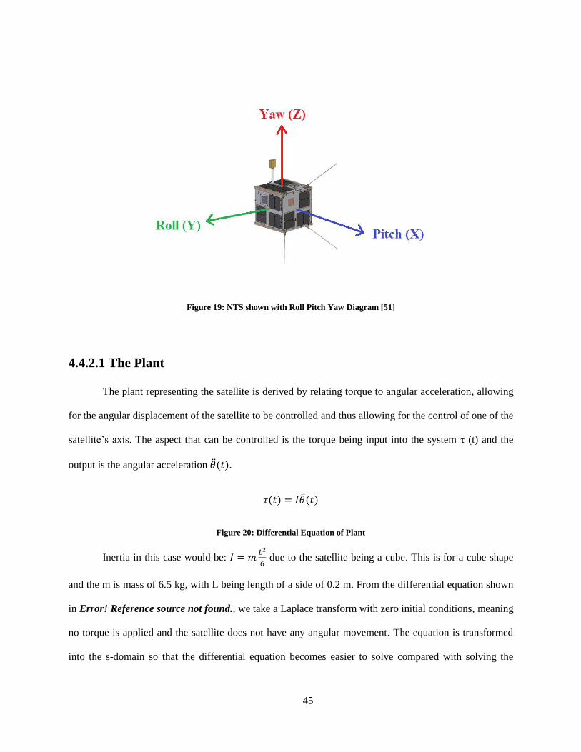
45
Figure 19: NTS shown with Roll Pitch Yaw Diagram [51]
4.4.2.1 The Plant
The plant representing the satellite is derived by relating torque to angular acceleration, allowing
for the angular displacement of the satellite to be controlled and thus allowing for the control of one of the
satellite’s axis. The aspect that can be controlled is the torque being input into the system τ (t) and the
output is the angular acceleration .
Figure 20: Differential Equation of Plant
Inertia in this case would be:
due to the satellite being a cube. This is for a cube shape
and the m is mass of 6.5 kg, with L being length of a side of 0.2 m. From the differential equation shown
in Error! Reference source not found., we take a Laplace transform with zero initial conditions, meaning
no torque is applied and the satellite does not have any angular movement. The equation is transformed
into the s-domain so that the differential equation becomes easier to solve compared with solving the
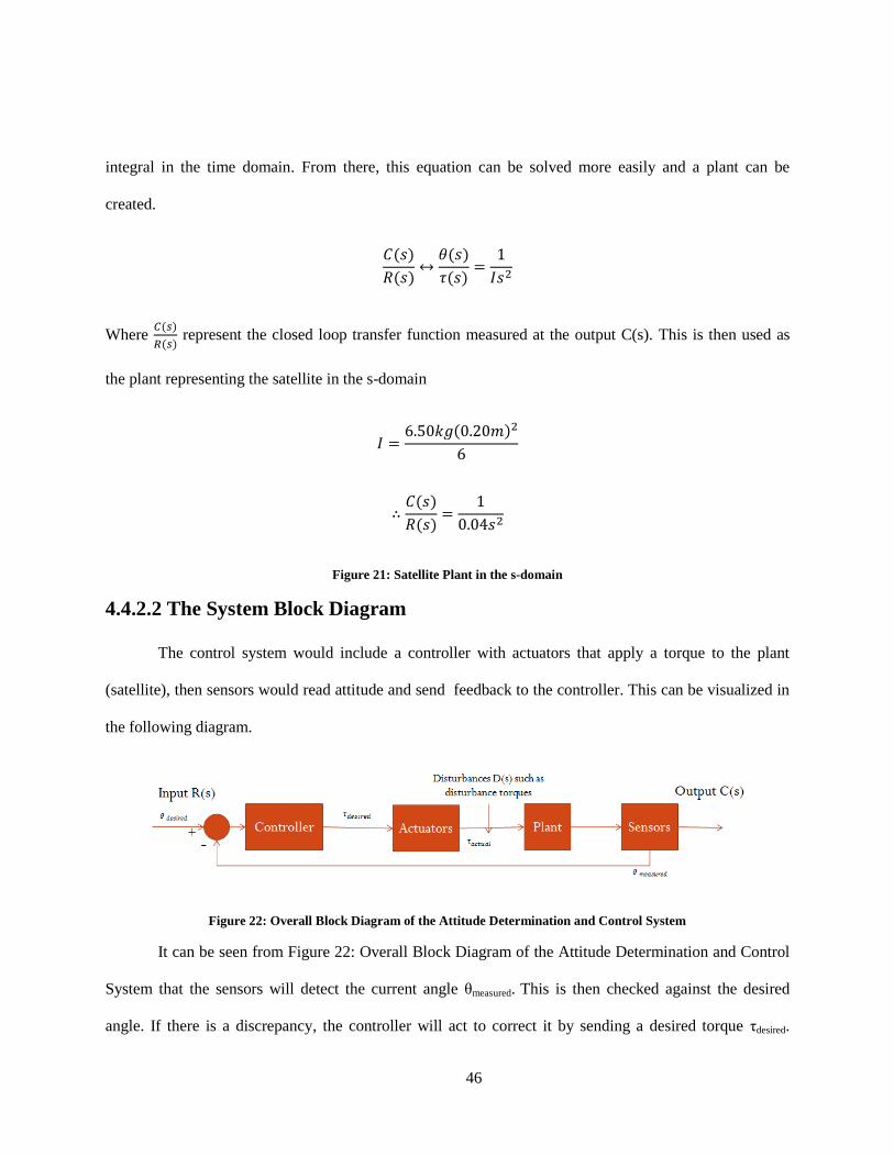
46
integral in the time domain. From there, this equation can be solved more easily and a plant can be
created.
Where
represent the closed loop transfer function measured at the output C(s). This is then used as
the plant representing the satellite in the s-domain
Figure 21: Satellite Plant in the s-domain
4.4.2.2 The System Block Diagram
The control system would include a controller with actuators that apply a torque to the plant
(satellite), then sensors would read attitude and send feedback to the controller. This can be visualized in
the following diagram.
Figure 22: Overall Block Diagram of the Attitude Determination and Control System
It can be seen from Figure 22: Overall Block Diagram of the Attitude Determination and Control
System that the sensors will detect the current angle θmeasured. This is then checked against the desired
angle. If there is a discrepancy, the controller will act to correct it by sending a desired torque τdesired.
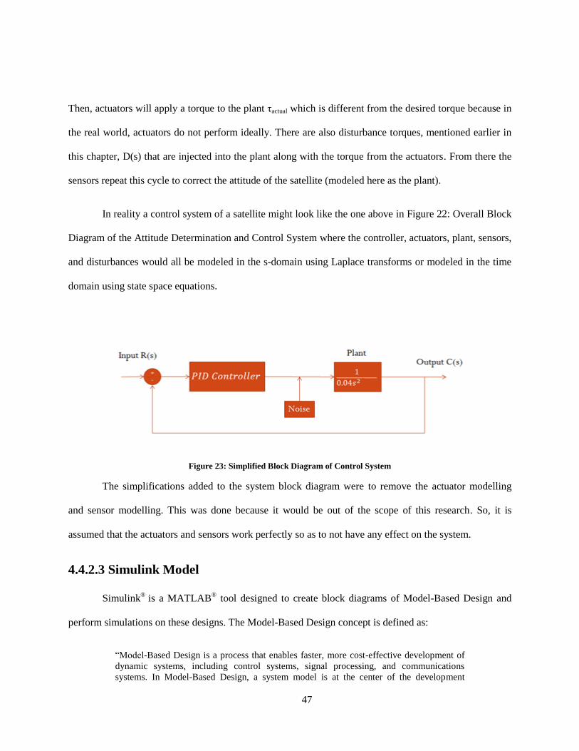
47
Then, actuators will apply a torque to the plant τactual which is different from the desired torque because in
the real world, actuators do not perform ideally. There are also disturbance torques, mentioned earlier in
this chapter, D(s) that are injected into the plant along with the torque from the actuators. From there the
sensors repeat this cycle to correct the attitude of the satellite (modeled here as the plant).
In reality a control system of a satellite might look like the one above in Figure 22: Overall Block
Diagram of the Attitude Determination and Control System where the controller, actuators, plant, sensors,
and disturbances would all be modeled in the s-domain using Laplace transforms or modeled in the time
domain using state space equations.
Figure 23: Simplified Block Diagram of Control System
The simplifications added to the system block diagram were to remove the actuator modelling
and sensor modelling. This was done because it would be out of the scope of this research. So, it is
assumed that the actuators and sensors work perfectly so as to not have any effect on the system.
4.4.2.3 Simulink Model
Simulink® is a MATLAB
® tool designed to create block diagrams of Model-Based Design and
perform simulations on these designs. The Model-Based Design concept is defined as:
“Model-Based Design is a process that enables faster, more cost-effective development of
dynamic systems, including control systems, signal processing, and communications
systems. In Model-Based Design, a system model is at the center of the development
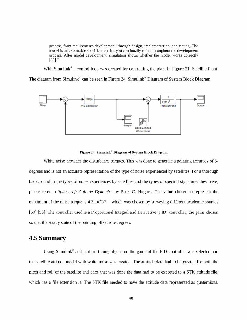
48
process, from requirements development, through design, implementation, and testing. The
model is an executable specification that you continually refine throughout the development
process. After model development, simulation shows whether the model works correctly
[52].”
With Simulink® a control loop was created for controlling the plant in Figure 21: Satellite Plant.
The diagram from Simulink® can be seen in Figure 24: Simulink
® Diagram of System Block Diagram.
Figure 24: Simulink® Diagram of System Block Diagram
White noise provides the disturbance torques. This was done to generate a pointing accuracy of 5-
degrees and is not an accurate representation of the type of noise experienced by satellites. For a thorough
background in the types of noise experiences by satellites and the types of spectral signatures they have,
please refer to Spacecraft Attitude Dynamics by Peter C. Hughes. The value chosen to represent the
maximum of the noise torque is 4.3 10-6
N which was chosen by surveying different academic sources
[50] [53]. The controller used is a Proportional Integral and Derivative (PID) controller, the gains chosen
so that the steady state of the pointing offset is 5-degrees.
4.5 Summary
Using Simulink® and built-in tuning algorithm the gains of the PID controller was selected and
the satellite attitude model with white noise was created. The attitude data had to be created for both the
pitch and roll of the satellite and once that was done the data had to be exported to a STK attitude file,
which has a file extension .a. The STK file needed to have the attitude data represented as quaternions,
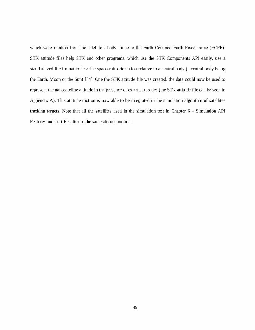
49
which were rotation from the satellite’s body frame to the Earth Centered Earth Fixed frame (ECEF).
STK attitude files help STK and other programs, which use the STK Components API easily, use a
standardized file format to describe spacecraft orientation relative to a central body (a central body being
the Earth, Moon or the Sun) [54]. One the STK attitude file was created, the data could now be used to
represent the nanosatellite attitude in the presence of external torques (the STK attitude file can be seen in
Appendix A). This attitude motion is now able to be integrated in the simulation algorithm of satellites
tracking targets. Note that all the satellites used in the simulation test in Chapter 6 – Simulation API
Features and Test Results use the same attitude motion.
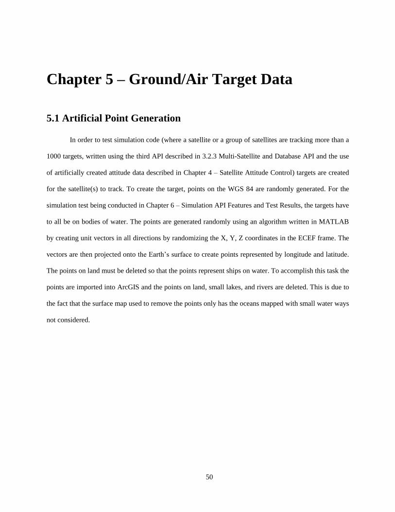
50
Chapter 5 – Ground/Air Target Data
5.1 Artificial Point Generation
In order to test simulation code (where a satellite or a group of satellites are tracking more than a
1000 targets, written using the third API described in 3.2.3 Multi-Satellite and Database API and the use
of artificially created attitude data described in Chapter 4 – Satellite Attitude Control) targets are created
for the satellite(s) to track. To create the target, points on the WGS 84 are randomly generated. For the
simulation test being conducted in Chapter 6 – Simulation API Features and Test Results, the targets have
to all be on bodies of water. The points are generated randomly using an algorithm written in MATLAB
by creating unit vectors in all directions by randomizing the X, Y, Z coordinates in the ECEF frame. The
vectors are then projected onto the Earth’s surface to create points represented by longitude and latitude.
The points on land must be deleted so that the points represent ships on water. To accomplish this task the
points are imported into ArcGIS and the points on land, small lakes, and rivers are deleted. This is due to
the fact that the surface map used to remove the points only has the oceans mapped with small water ways
not considered.
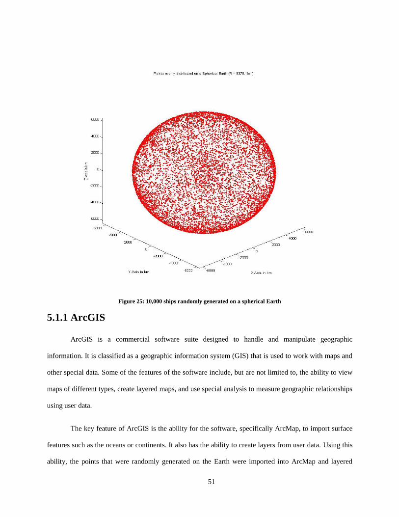
51
Figure 25: 10,000 ships randomly generated on a spherical Earth
5.1.1 ArcGIS
ArcGIS is a commercial software suite designed to handle and manipulate geographic
information. It is classified as a geographic information system (GIS) that is used to work with maps and
other special data. Some of the features of the software include, but are not limited to, the ability to view
maps of different types, create layered maps, and use special analysis to measure geographic relationships
using user data.
The key feature of ArcGIS is the ability for the software, specifically ArcMap, to import surface
features such as the oceans or continents. It also has the ability to create layers from user data. Using this
ability, the points that were randomly generated on the Earth were imported into ArcMap and layered
52
over the oceans. After the points were layered over the oceans, all points on land masses were removed,
leaving 100,000 points on the oceans.
Figure 26: Points (green) only on oceans in ArcMap
The points on the ocean were then exported into a text file from which the simulation software
developed - using the third API - could read in the data and perform a tracking simulation. The ships do
not represent a realistic distribution but for the purpose of testing the simulation, the placement of the
ships would not matter. As mentioned in sections 5.2 Real World Target Data and 5.3 Simulated Sources
of Data, other sources of target data, especially for ships, exist and they would be better in performing a
more realistic simulation with superior target distribution.
5.2 Real World Target Data
Target data can be obtained for two types of targets: aircraft and ship traffic. Aircraft traffic is
logged by a number of agencies including the Federal Aviation Administration (FAA), North American
Aerospace Defense Command, and NAV Canada. Most of the data is aggregated using sources such as
53
ADS-B (Automatic dependent surveillance-broadcast), MLAT (Multilateration Surveillance), and FAA
(for air traffic in the US) [55].
For ship traffic data, the CLS Group, which is a subsidiary of the French Space Agency,
is a source of this type of data. COMDEV and ORBCOMM are commercial providers of AIS data using
satellites to gather the data.
5.3 Simulated Sources of Data
Target data for vessels do not always have to be retrieved from real data. Vessel traffic is used in
many other simulations for purposes of training personnel for maritime services, planning future
infrastructure, and traffic management [56] [57]. There are many commercial simulations called VTS
(Vessel Traffic Service) Simulations along with simulations developed for research purposes that simulate
vessel traffic in many different ways. One of these simulators is by Kongsberg Maritime, which produces
a VTS. The VTS is used to generate realistic traffic patterns with realistic communications for operators
[58]. Some other companies that develop vessel traffic simulators are TRANSAS, SIMPLUS, and BMT
ISIS. As mentioned before, the purpose of these simulations is to be used in training sessions for marine
operators or for traffic management.
There are also some simulations created as part of research at universities around the world. One
simulation in particular, created at the University of Antwerp, is a simulation to create port traffic around
Antwerp, Belgium. The simulation was to be modular in design and took into consideration many
variables, some of which include the type of vessel, boundaries of the waterways, the tide, weather
patterns and many more. The simulation created was to be used to make decisions when changing
infrastructure [56]. Some of these simulations are created to mitigate piracy as well, such as the
simulation created at the Czech Technical University. It simulates merchant vessels and pirate vessels,
and models them using real world AIS data [59].
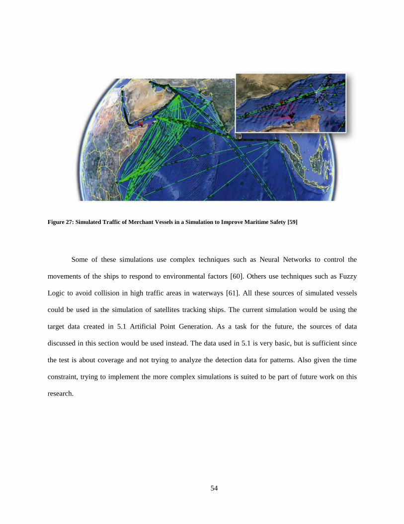
54
Figure 27: Simulated Traffic of Merchant Vessels in a Simulation to Improve Maritime Safety [59]
Some of these simulations use complex techniques such as Neural Networks to control the
movements of the ships to respond to environmental factors [60]. Others use techniques such as Fuzzy
Logic to avoid collision in high traffic areas in waterways [61]. All these sources of simulated vessels
could be used in the simulation of satellites tracking ships. The current simulation would be using the
target data created in 5.1 Artificial Point Generation. As a task for the future, the sources of data
discussed in this section would be used instead. The data used in 5.1 is very basic, but is sufficient since
the test is about coverage and not trying to analyze the detection data for patterns. Also given the time
constraint, trying to implement the more complex simulations is suited to be part of future work on this
research.
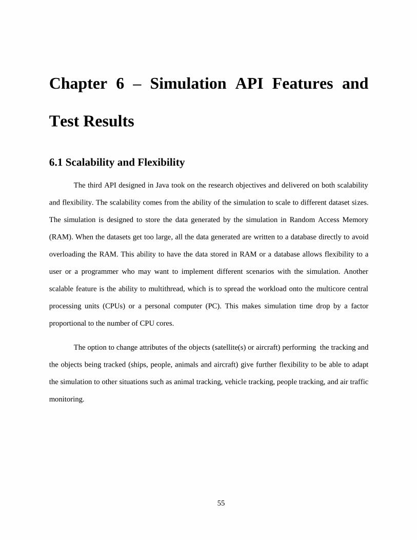
55
Chapter 6 – Simulation API Features and
Test Results
6.1 Scalability and Flexibility
The third API designed in Java took on the research objectives and delivered on both scalability
and flexibility. The scalability comes from the ability of the simulation to scale to different dataset sizes.
The simulation is designed to store the data generated by the simulation in Random Access Memory
(RAM). When the datasets get too large, all the data generated are written to a database directly to avoid
overloading the RAM. This ability to have the data stored in RAM or a database allows flexibility to a
user or a programmer who may want to implement different scenarios with the simulation. Another
scalable feature is the ability to multithread, which is to spread the workload onto the multicore central
processing units (CPUs) or a personal computer (PC). This makes simulation time drop by a factor
proportional to the number of CPU cores.
The option to change attributes of the objects (satellite(s) or aircraft) performing the tracking and
the objects being tracked (ships, people, animals and aircraft) give further flexibility to be able to adapt
the simulation to other situations such as animal tracking, vehicle tracking, people tracking, and air traffic
monitoring.
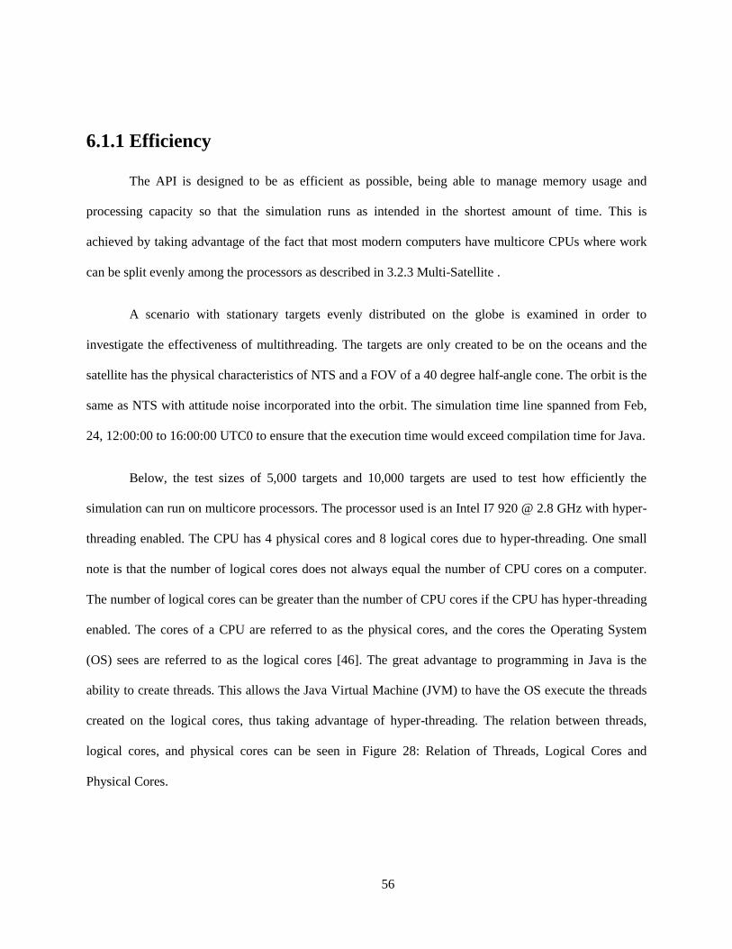
56
6.1.1 Efficiency
The API is designed to be as efficient as possible, being able to manage memory usage and
processing capacity so that the simulation runs as intended in the shortest amount of time. This is
achieved by taking advantage of the fact that most modern computers have multicore CPUs where work
can be split evenly among the processors as described in 3.2.3 Multi-Satellite .
A scenario with stationary targets evenly distributed on the globe is examined in order to
investigate the effectiveness of multithreading. The targets are only created to be on the oceans and the
satellite has the physical characteristics of NTS and a FOV of a 40 degree half-angle cone. The orbit is the
same as NTS with attitude noise incorporated into the orbit. The simulation time line spanned from Feb,
24, 12:00:00 to 16:00:00 UTC0 to ensure that the execution time would exceed compilation time for Java.
Below, the test sizes of 5,000 targets and 10,000 targets are used to test how efficiently the
simulation can run on multicore processors. The processor used is an Intel I7 920 @ 2.8 GHz with hyper-
threading enabled. The CPU has 4 physical cores and 8 logical cores due to hyper-threading. One small
note is that the number of logical cores does not always equal the number of CPU cores on a computer.
The number of logical cores can be greater than the number of CPU cores if the CPU has hyper-threading
enabled. The cores of a CPU are referred to as the physical cores, and the cores the Operating System
(OS) sees are referred to as the logical cores [46]. The great advantage to programming in Java is the
ability to create threads. This allows the Java Virtual Machine (JVM) to have the OS execute the threads
created on the logical cores, thus taking advantage of hyper-threading. The relation between threads,
logical cores, and physical cores can be seen in Figure 28: Relation of Threads, Logical Cores and
Physical Cores.
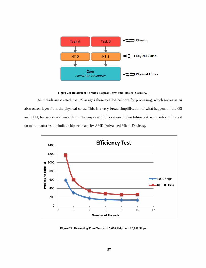
57
Figure 28: Relation of Threads, Logical Cores and Physical Cores [62]
As threads are created, the OS assigns these to a logical core for processing, which serves as an
abstraction layer from the physical cores. This is a very broad simplification of what happens in the OS
and CPU, but works well enough for the purposes of this research. One future task is to perform this test
on more platforms, including chipsets made by AMD (Advanced Micro-Devices).
Figure 29: Processing Time Test with 5,000 Ships and 10,000 Ships
0
200
400
600
800
1000
1200
1400
0 2 4 6 8 10 12
Pro
cess
ing
Tim
e (
s)
Number of Threads
Efficiency Test
5,000 Ships
10,000 Ships
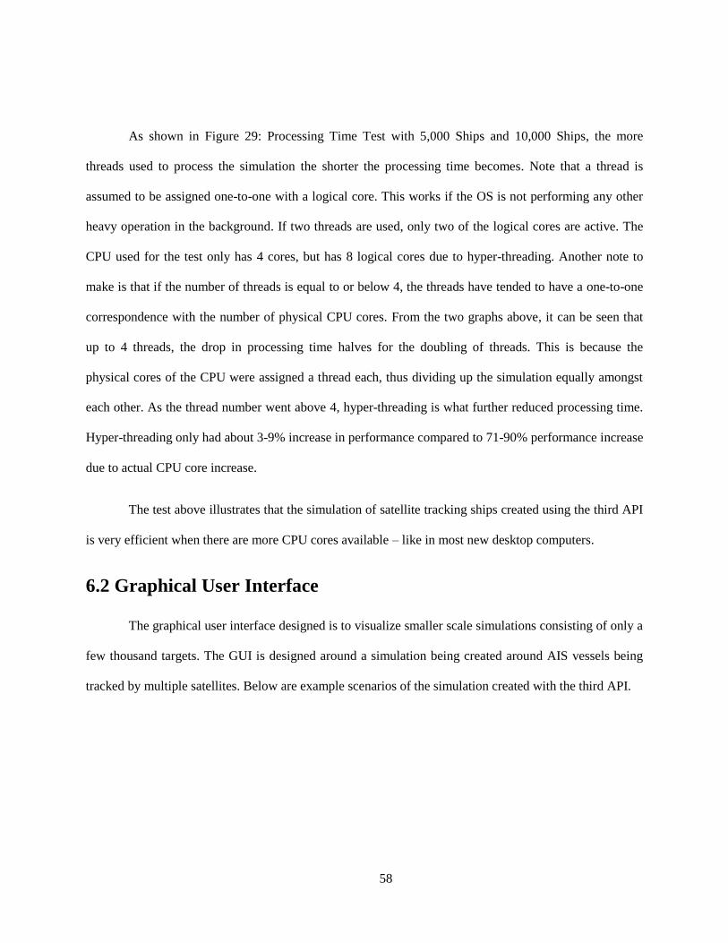
58
As shown in Figure 29: Processing Time Test with 5,000 Ships and 10,000 Ships, the more
threads used to process the simulation the shorter the processing time becomes. Note that a thread is
assumed to be assigned one-to-one with a logical core. This works if the OS is not performing any other
heavy operation in the background. If two threads are used, only two of the logical cores are active. The
CPU used for the test only has 4 cores, but has 8 logical cores due to hyper-threading. Another note to
make is that if the number of threads is equal to or below 4, the threads have tended to have a one-to-one
correspondence with the number of physical CPU cores. From the two graphs above, it can be seen that
up to 4 threads, the drop in processing time halves for the doubling of threads. This is because the
physical cores of the CPU were assigned a thread each, thus dividing up the simulation equally amongst
each other. As the thread number went above 4, hyper-threading is what further reduced processing time.
Hyper-threading only had about 3-9% increase in performance compared to 71-90% performance increase
due to actual CPU core increase.
The test above illustrates that the simulation of satellite tracking ships created using the third API
is very efficient when there are more CPU cores available – like in most new desktop computers.
6.2 Graphical User Interface
The graphical user interface designed is to visualize smaller scale simulations consisting of only a
few thousand targets. The GUI is designed around a simulation being created around AIS vessels being
tracked by multiple satellites. Below are example scenarios of the simulation created with the third API.
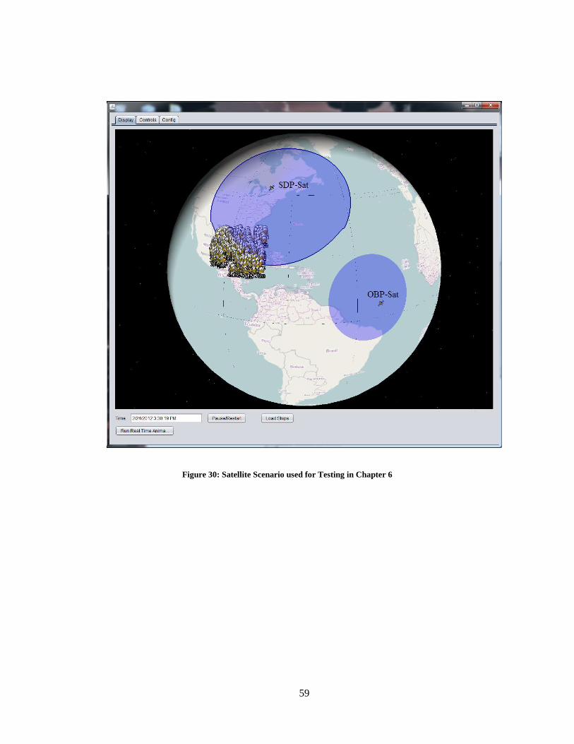
59
Figure 30: Satellite Scenario used for Testing in Chapter 6
60
Figure 31: Example simulation with targets randomly generated on Earth
The purpose of the GUI was to help the user visualize the simulation so that data can be inspected
visually to make sure that text data are accurate. So, if a target was shown to be detected by a satellite
using the simulation, the GUI could be used to visually inspect it if indeed a target was within a satellite’s
FOV.
6.3 Testing and Results
To test the simulation of a scenario with a specific problem encountered in the space industry,
satellite AIS (Automatic Identification Signals) providers will be considered. Such a problem is coverage
61
of AIS signals from ships in a certain area of the world. When trying to track ships using AIS signals, the
high-traffic areas (such as the Gulf of Mexico, Persian Gulf or Sea of Japan) are very important due to
safety and sovereignty.
There are several aspects that will be tested from the scenario mentioned above such as the orbit
of the satellite, the number of satellites, and the technology used in the receiver of the satellite. The AIS
receivers have major influences on the performance of an AIS satellite. From the providers of AIS data
there are two types of AIS receivers used in the industry. The first is onboard processing (OBP) of AIS
data, which is described as follows:
“This processing mode essentially decodes AIS messages directly on the satellite using
narrow band filters and stores the messages on the spacecraft for later downlink to the
nearest Earth Station. It does not require any special processing and is effective in very low
density areas, such as the middle of the Pacific Ocean. However, the detection probability
is low in areas where the satellite footprint (~5,000 km in diameter) contains a ship density
exceeding about 500 ships as it become likely that all of the AIS message slots are being
used by more than ship at a time. This effect results in a time slot collision and it becomes
much more difficult to successfully decode [63].”
This method of processing is what the rest of the industry uses, but exactEarth has developed its
own processing which is called spectral de-collision processing (SDP) and is described as follows:
“SDP requires the capture of the AIS RF spectrum and processing of that spectrum
using highly specialized algorithms to successfully decode AIS reports. With SDP
the first pass detection ability is high even within high ship density areas, thus
quickly achieving effective operational maritime capability. Statistical analysis has
shown that the improvement in FPD (First Pass Detection) for this detection
methodology in highly dense shipping areas can result in significantly higher ship
detection, number of position reports received (for behavioral modeling and
predictive algorithms), and reception of multipart (multi-slot) messages containing
static and voyage related information [63].”
The exact details of the performance of the receivers are proprietary, but there is a performance
chart used by COM DEV which compares the two types of receivers.
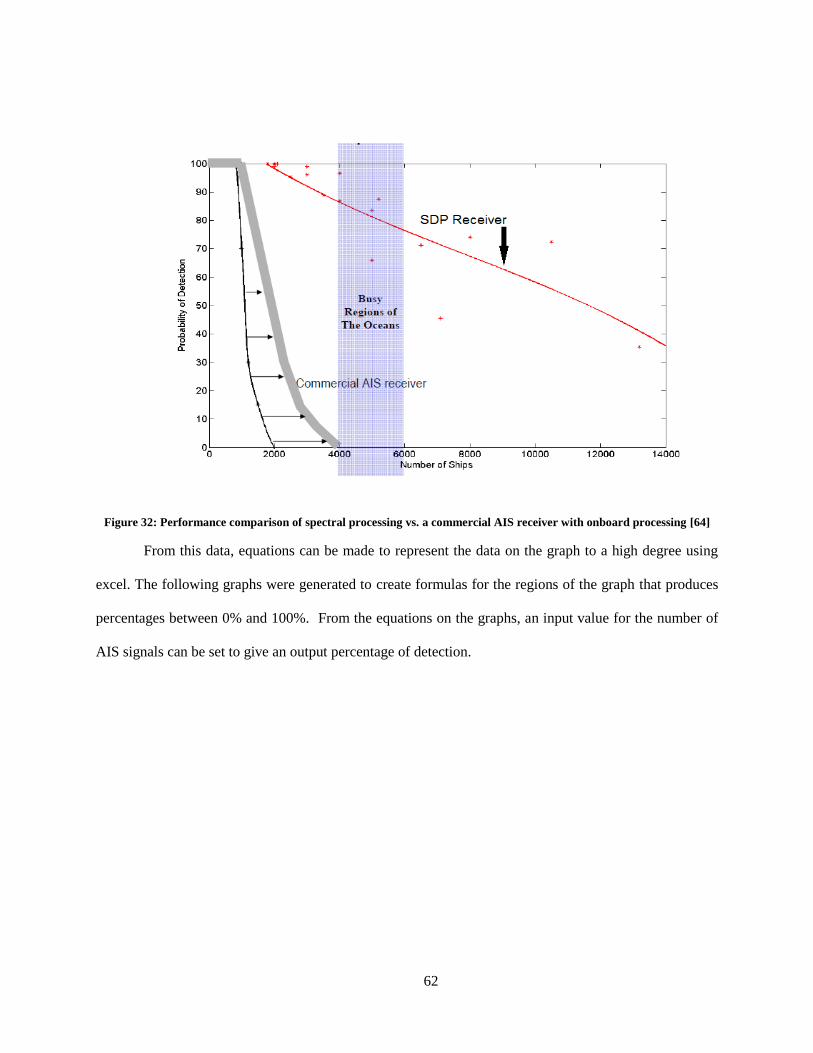
62
Figure 32: Performance comparison of spectral processing vs. a commercial AIS receiver with onboard processing [64]
From this data, equations can be made to represent the data on the graph to a high degree using
excel. The following graphs were generated to create formulas for the regions of the graph that produces
percentages between 0% and 100%. From the equations on the graphs, an input value for the number of
AIS signals can be set to give an output percentage of detection.
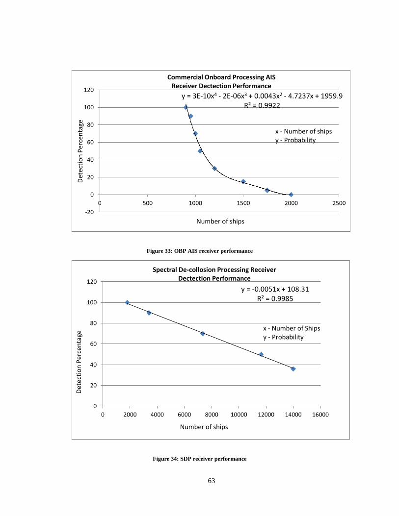
63
Figure 33: OBP AIS receiver performance
Figure 34: SDP receiver performance
y = 3E-10x4 - 2E-06x3 + 0.0043x2 - 4.7237x + 1959.9 R² = 0.9922
-20
0
20
40
60
80
100
120
0 500 1000 1500 2000 2500
Commercial Onboard Processing AIS Receiver Dectection Performance
Det
ecti
on
Per
cen
tage
Number of ships
x - Number of ships y - Probability
y = -0.0051x + 108.31 R² = 0.9985
0
20
40
60
80
100
120
0 2000 4000 6000 8000 10000 12000 14000 16000
Number of ships
Det
ecti
on
Per
cen
tage
Spectral De-collosion Processing Receiver Dectection Performance
x - Number of Ships y - Probability
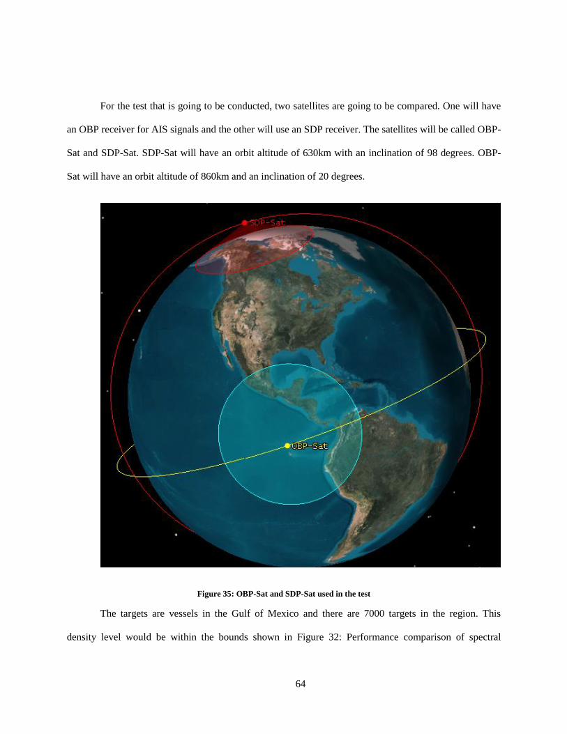
64
For the test that is going to be conducted, two satellites are going to be compared. One will have
an OBP receiver for AIS signals and the other will use an SDP receiver. The satellites will be called OBP-
Sat and SDP-Sat. SDP-Sat will have an orbit altitude of 630km with an inclination of 98 degrees. OBP-
Sat will have an orbit altitude of 860km and an inclination of 20 degrees.
Figure 35: OBP-Sat and SDP-Sat used in the test
The targets are vessels in the Gulf of Mexico and there are 7000 targets in the region. This
density level would be within the bounds shown in Figure 32: Performance comparison of spectral
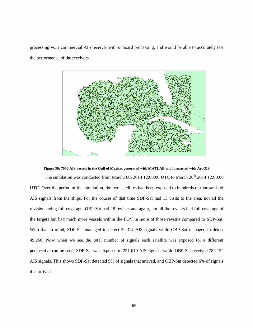
65
processing vs. a commercial AIS receiver with onboard processing, and would be able to accurately test
the performance of the receivers.
Figure 36: 7000 AIS vessels in the Gulf of Mexico, generated with MATLAB and formatted with ArcGIS
The simulation was conducted from March16th 2014 12:00:00 UTC to March 20th 2014 12:00:00
UTC. Over the period of the simulation, the two satellites had been exposed to hundreds of thousands of
AIS signals from the ships. For the course of that time SDP-Sat had 15 visits to the area, not all the
revisits having full coverage. OBP-Sat had 28 revisits and again, not all the revisits had full coverage of
the targets but had much more vessels within the FOV in more of those revisits compared to SDP-Sat.
With that in mind, SDP-Sat managed to detect 22,314 AIS signals while OBP-Sat managed to detect
49,266. Now when we see the total number of signals each satellite was exposed to, a different
perspective can be seen. SDP-Sat was exposed to 251,619 AIS signals, while OBP-Sat received 782,152
AIS signals. This shows SDP-Sat detected 9% of signals that arrived, and OBP-Sat detected 6% of signals
that arrived.
66
With this test it is seen that the performance of the satellites is dependent on several factors and
the detection figures show how affective certain aspects such as orbit parameters and payload parameters
are. OBP-Sat had the advantage of having a low inclination – which means that it would only see AIS
signals in lower latitudes such as the AIS signals from ships in the Gulf of Mexico, while SDP-Sat had
the better receiver and better coverage away from the equator due to the high inclination. With this kind
of information, an AIS data provider can analyze the competition and have insight into their weaknesses,
the client also being able to choose AIS data providers depending on their needs.
Revisit Time Test
In this test we will be checking the average revisit time over a 24-hour simulation period. The
data set used is of 7000 ships in the Gulf of Mexico, the same dataset which is shown in Figure 36: 7000
AIS vessels in the Gulf of Mexico, generated with MATLAB and formatted with ArcGIS. The test will
use 9 satellites with polar orbits, while the 10th satellite will have the same orbit as OBP-Sat in the
previous example.
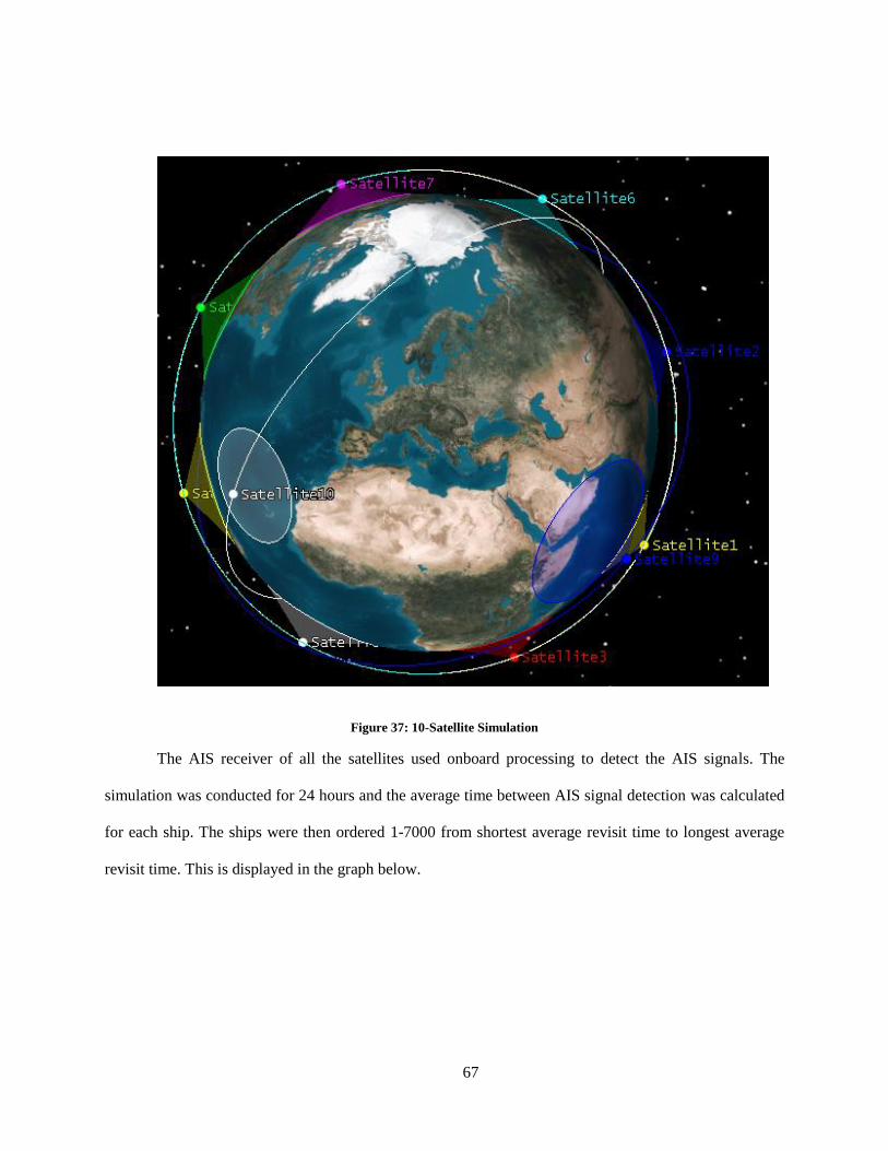
67
Figure 37: 10-Satellite Simulation
The AIS receiver of all the satellites used onboard processing to detect the AIS signals. The
simulation was conducted for 24 hours and the average time between AIS signal detection was calculated
for each ship. The ships were then ordered 1-7000 from shortest average revisit time to longest average
revisit time. This is displayed in the graph below.
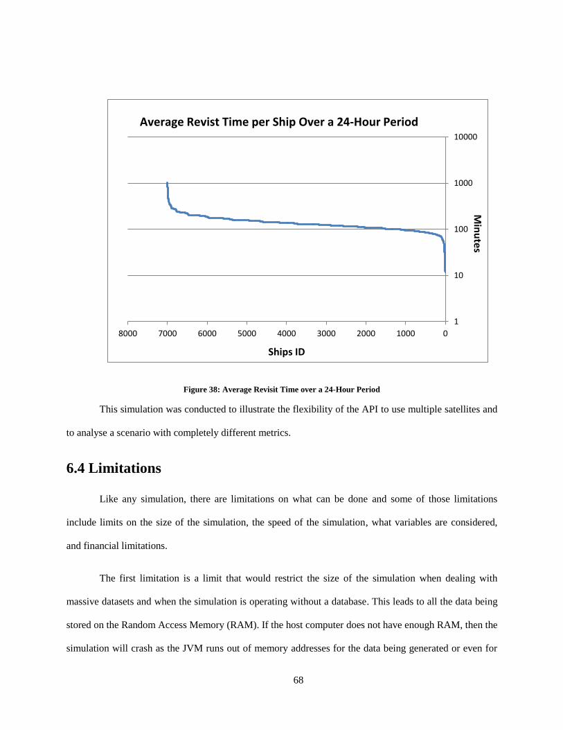
68
Figure 38: Average Revisit Time over a 24-Hour Period
This simulation was conducted to illustrate the flexibility of the API to use multiple satellites and
to analyse a scenario with completely different metrics.
6.4 Limitations
Like any simulation, there are limitations on what can be done and some of those limitations
include limits on the size of the simulation, the speed of the simulation, what variables are considered,
and financial limitations.
The first limitation is a limit that would restrict the size of the simulation when dealing with
massive datasets and when the simulation is operating without a database. This leads to all the data being
stored on the Random Access Memory (RAM). If the host computer does not have enough RAM, then the
simulation will crash as the JVM runs out of memory addresses for the data being generated or even for
1
10
100
1000
10000
010002000300040005000600070008000
Average Revist Time per Ship Over a 24-Hour Period
Ships ID
Min
ute
s
69
storing the targets themselves. The usual size for computer RAM in 2013 tends to be around 4 gigabytes
(GB) and the limit imposed by current operating systems such as Microsoft Windows™ (OSs) is 192 GB
[65].
The speed of the simulation is limited by either the CPU that is not able to process information
fast enough or the disk/database to which data is being written to. Usually the writing to disk tends to be
the bottleneck in the system.
Then there are the limitations due to abstractions in the simulation. There is only certain depth in
detail that a programmer can get to where the computation involved becomes massive in scale or, the time
involved to program the simulation is too difficult and time consuming. For example, the satellite is going
to be treated as a point mass when propagating the orbit and a simplified body for simulating the attitude.
A finite element model of the satellites is not required because it would not provide any benefit to the
simulation to have that kind of complexity involved. This leads to the next point of all this abstraction:
reducing the number of variables considered for the simulation. The variables considered cover the
satellite path, satellite attitude, the FOV shapes, the ship path, and transmitter timing that determines
when a signal is sent out. Signal propagation is not modeled in terms of a spectral signal but instead as an
instantaneous propagation that is received at the receiver. These simplifications reduce some of the depth
of the simulation but for the cases considered, they would not provide a benefit. For example in
simulating the AIS signals, it is proven that VHF signals can reach the satellite at low earth orbits, so it
would not be beneficial to incorporate atmospheric attenuation. Instead, the assumption is made that the
signal will reach the satellite.
Finally there are the financial limitations of the simulation because of the software and hardware
that are required to run the simulation and use the API. Computer hardware is required to run simulations
and there may be dollar costs associated with using a database.
70
Chapter 7 – Future Work and Conclusion
7.1 Future Work
There are many aspects of the simulation that can be improved for reliability, realism, and user
friendliness. Some of them obvious like improving the graphical user interface (GUI) so that a user will
find it more intuitive. This can be done using a cleaner menu system and adding in more functions such as
the ability to create FOV in the GUI.
7.1.1 Transmitter Modelling and Receiver Modelling
As the simulation is developed into the future, it would be crucial to model the transmitters and
receivers based on real world conditions. This would greatly apply to a ship traffic simulation using AIS
based transmitters and satellites using AIS receivers. Some of the complexities that would have to be
incorporated into the simulation would be: the time delay of the signal, message collisions on the receiver
side due to the coverage of many SOTDMA cells, attenuation due to the atmosphere and distance causing
low signal-to-noise ratio (SNR), signals taking multiple paths due to the atmosphere reflection and
refractions (especially true for AIS signals being transmitted in the VHF region of the spectrum), and
Doppler effects, to name the major factors [27].
7.1.2 Artificial Target Generation
The generation of targets at this point has been a random point generation algorithm. If the points
need to be on the ocean or on land, ArcGIS has to be used in order to remove the unwanted points. This
method of point generation is not very useful for creating targets such as ships following shipping routes
71
since they are equally spread over the planet and they do not follow the paths that are similar to the ones
in the real world.
One way to improve this is to create another separate simulation which can generate proper traffic
for ships as mentioned in section 5.3 Simulated Sources of Data or aircraft. This would be done by
gathering all the air traffic pathways and ship traffic pathways and generating points that would travel
back and forth on these channels. This would greatly improve the realism in the simulation and for a
person or group interested in a certain area of the Earth, it would be useful to generate data relevant to
that location. An example of this is a port city where there would be a heavy concentration of ships
coming and going and travel patterns of these ships would be greatly different to that of ships in open
water. This kind of simulation could be based on the models that are mentioned in Chapter 5 or could be
derived from a combination of simulations.
7.1.3 GUI Improvement
The graphical user interface at this point is only useful for visualizing a simulation containing
only a few thousand targets. To improve the simulation, more work has to be put into improving the look
of the GUI and adding in more features. Some of the features that need to be added in the future are to
create and run the simulation using the GUI only. The ability to supply a file to run the simulation (like a
configuration file), the ability to provide more graphical options such as different central bodies (Earth,
Mars and the Moon are central bodies), and better controls to change the speed of the simulation are also
to be added in the future. The GUI should be similar to the Satellite Toolkit interface, but without so
many of the options and complexities.
72
7.2 Final Remarks
With the objectives that were listed in section 1.2 Research Objectives, all the numbered points
have been mentioned. Starting with scalability, the API from the simulation built is able to scale to large
number of targets and tracking assets. The flexibility of the simulation permits different configurations of
the satellite, like the test conducted in 6.3 Test, allowing the comparison of two very different satellites.
The efficiency of the simulation was achieved by multithreading the detection of targets by the satellites.
The test shown in 6.1 Scalability and Flexibility shows the flexibility and efficiency that has been
achieved. The ease of use has not been demonstrated in a test but is displayed in the class libraries which
are contained in the API created, shown in section 3.2.3 Multi-Satellite and Database . The final objective
is achieved by including use of STK Components, which ensures that a tried and tested platform is used
for some aspects of the simulation.
Throughout this research a simulation has been created to track a large number of targets (ranging
in the thousands) with a group of satellites with different configurations. This simulation has been created
with the API that was created in Java with the use of the Java standard library, the STK Components API,
the JDBC driver to connect to databases, and the use of the MongoDB java driver. It has resulted in a
simulation that is modular and efficient. It has also led to the creation of a simple Graphical User
Interface (GUI) for a user to use in order to visualize the simulation they have conducted. The aspects of
the satellites that were used such as the attitude and field of view have also been incorporated to include a
deep level of configurability to the simulation.
In conclusion, this research has set out to accomplish a list of objectives and has met all these
targets. What it has also shown is the need for this sort of simulation in the face of challenges faced by
many industries, such as the aerospace industry in choosing a satellite constellation to provide continuous
tracking for aircraft. This is one of the many different problems that can be solved. For the shipping
73
industry the problem of coverage also exists, and finding the correct AIS data provider or getting a
combination of AIS data providers would be useful to maximize coverage and minimize cost. From what
is mentioned in section 2.1 Tracking from a Satellite about human tracking, animal tracking, and tracking
of motor vehicles, the use of a simulation like this can really help researchers further in development,
especially with this simulation and what is shown it is capable of.
7.3 Contributions
The contributions of this research are summarised below:
1. The application of a large scale simulation of satellites tracking a large number of targets was
examined. Specifically, the large target data involved in vehicular traffic, air traffic, ship traffic,
animal tracking, and tracking people were considered.
2. The points on the oceans to represent ships were created to simulate the marine traffic in target
areas. This simple ship traffic simulation algorithm was used to evaluate the performance of the
simulation algorithm. For future consideration, a survey of commercial marine traffic simulation
algorithms was presented for comparison.
3. The basic attitude simulation algorithm to estimate a typical nanosatellite motion in two-axis was
developed. The external torques, including gravitational tidal forces, aerodynamic drag due to the
atmosphere, drag due to solar wind, and torque due to the magnetic field were accounted for and
included in the simulation and a suitable controller was designed to represent attitude profile of a
6.5-kg nanosatellite in low earth orbit. From this simulation, attitude data is generated and
formatted into an STK attitude file, to be used with STK or with the developed second and third
API model mention in sections 3.2.2 Single Satellite Non-Spherical Earth and Non-Circular Orbit
API and 3.2.3 Multi-Satellite and Database API.
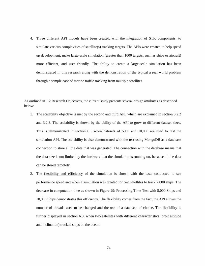
74
4. Three different API models have been created, with the integration of STK components, to
simulate various complexities of satellite(s) tracking targets. The APIs were created to help speed
up development, make large-scale simulation (greater than 1000 targets, such as ships or aircraft)
more efficient, and user friendly. The ability to create a large-scale simulation has been
demonstrated in this research along with the demonstration of the typical a real world problem
through a sample case of marine traffic tracking from multiple satellites
As outlined in 1.2 Research Objectives, the current study presents several design attributes as described
below:
1. The scalability objective is met by the second and third API, which are explained in section 3.2.2
and 3.2.3. The scalability is shown by the ability of the API to grow to different dataset sizes.
This is demonstrated in section 6.1 when datasets of 5000 and 10,000 are used to test the
simulation API. The scalability is also demonstrated with the test using MongoDB as a database
connection to store all the data that was generated. The connection with the database means that
the data size is not limited by the hardware that the simulation is running on, because all the data
can be stored remotely.
2. The flexibility and efficiency of the simulation is shown with the tests conducted to see
performance speed and when a simulation was created for two satellites to track 7,000 ships. The
decrease in computation time as shown in Figure 29: Processing Time Test with 5,000 Ships and
10,000 Ships demonstrates this efficiency. The flexibility comes from the fact, the API allows the
number of threads used to be changed and the use of a database of choice. The flexibility is
further displayed in section 6.3, when two satellites with different characteristics (orbit altitude
and inclination) tracked ships on the ocean.
75
3. The abstractions made with the third API to have objects to represent satellites and targets, so that
a user can quickly add assets, demonstrate the easy to understand nature of the API. The GUI
shown in Figure 30: Satellite Scenario used for Testing in Chapter 6 is created so a user can run a
simulation of a satellite tracking targets without having to write a simulation algorithm of their
own.
76
Bibliography 1. Gutierrez , Jordi. Implementation of a femto-satellite and mini-launcher. Barcelona : Polytechnic
University of Catalonia, 2010.
2. Defense Industry Daily. Small Is Beautiful: US Military Explores Use of Microsatellites. Defense
Industry Daily. [Online] Defense Industry Daily, June 30, 2011. [Cited: 7 2, 2013.]
http://www.defenseindustrydaily.com/Small-Is-Beautiful-US-Military-Explores-Use-of-Microsatellites-
06720/.
3. Cummings, John. Army nanosatellite on first flight. THe Official Homepage of The United States
Army. [Online] The United States Army, December 8, 2010. [Cited: January 20, 2014.]
http://www.army.mil/article/49115/army-nanosatellite-on-first-flight/.
4. Wertz, James R and Larson, Wiley J. Space Mission Analysis And Design. 3rd. New York :
Microcosm Press and Springer, 2010.
5. Kim, Jeongrae. Simulation Study of A Low-Low Satellite-to-Satellite Tracking Mission. Austin : The
University of Texas at Austin, 2000.
6. Coleshill, Elliott. AIS: Technology Development to Commercialization. CAISU. [Online] 2010.
[Cited: Augest 4, 2013.] http://www.caisu.org/nsaw/2010/presentations/ElliottColeshill.pdf.
7. New Simulation Approach for the Training Satellite Mission Control Teams. Innorta, Daniele and
Williams, Adam. Darmstadt : IEEE, 2007.
8. Astronautics, Best Practices Working Group Space Operations and Ssupport Technical
committee American Institute of Aeronautics and Space-OPS. The International Committee on
77
Technical Interchange for Space Mission Operations and Ground Data Systems. [Online] April 18, 2003.
[Cited: December 25, 2013.] http://www.spaceops.org/images/spaceops/SOSTC-BestPractices.pdf.
9. Real Time Three-Dimensional Simulation Platform for Satellite Mission Analysis. Hao, Huang, et al.
Beijing : IEEE, 2011.
10. Koyamada, Koji, Tamura, Shinsuke and Ono, Osamu. Systems Modeling and Simulation Theory
and Applications, Asia Simulation Conference 2006 . Tokyo : Springer, 2006. ISBN-10 4-431-49021-3.
11. Maritime traffic monitoring using a space-basedAIS receiver. Eriksen, Torkild, et al. Kjeller : s.n.,
May 30, 2005, Science Direct, pp. 1-2.
12. Roddy, Dennis. Orbital Elements. Satellite Communications. New York : Mcgraw-Hill Companies,
2006.
13. Curtis, Howard D. Preliminary Orbit Determination. Orbital Mechanics for Engineering Students .
Burlington : Elsevier Ltd., 2010.
14. Satellites for Research on Free-Roaming Animals. Buechner, Helmut K., et al. 24, s.l. : University
California Press, December 15, 1971, BioScience, Vol. 21, pp. 1201-1205.
15. U.S. Department of the Interior, U.S. Geological Survey. A Critique of Wildlife Radio-tracking.
Northern Prairie Wildlife Research Center. [Online] Auguest 3, 2006. [Cited: September 9, 2012.]
http://www.npwrc.usgs.gov/resource/wildlife/radiotrk/satell.htm.
16. Pepper, David. Woodcock Watch. Game & Wildlife Conservation Trust. [Online] 2013. [Cited:
September 29, 2013.] http://www.woodcockwatch.com/satellite-tags.php.
17. CLS Group. How it works. ARGOS. [Online] http://www.argos-system.org/web/en/67-how-it-
works.php.
78
18. Low-Cost Responsive Explotiation of Space by HAUSAT-2 Nano Satellite. Chang, Young Keun, et
al. Los Angeles : Hankuk Aviation University, South Korea, 2006. 4th Responsive Space Conference. pp.
1-2.
19. Brandy, Brian. Prisoners 'to be chipped like dogs'. The Independent. January 13, 2008, pp. 1-3.
20. Eternal Vigilance Inc.: The Satellite Tracking of Offenders in "Real Time". Nellis, Mike. s.l. : Taylor
& Francis Group, LLC, April 28, 2010, Journal of Technology in Human Services, pp. 23-27.
21. International Civil Aviation Organization. ICAO in Brief. International Civil Aviation
Organization. [Online] 2013. [Cited: 9 20, 2013.] http://www.icao.int/about-icao/Pages/default.aspx.
22. An autonomous, non-cooperative, wide-area Traffic Monitoring System using space-based Radar
(TRAMRAD). Hounam, D., et al. 2005, IEEE, pp. 1-2.
23. Charlton, Angela. thestar.com. [Online] July 7, 2009. [Cited: January 24, 2013.]
http://www.thestar.com/news/world/2009/07/07/air_france_crash_prompts_look_at_air_traffic_black_hol
es.html.
24. Boeing. Current Market Outlook 2013-2032. Boeing. [Online] 2013. [Cited: August 25, 2013.]
http://www.boeing.com/boeing/commercial/cmo/.
25. NAV CANADA. NAV CANADA. [Online] June 27, 2013. [Cited: August 23, 2013.]
http://www.navcanada.ca/navcanada.asp?Language=en&Content=ContentDefinitionFiles%5CNewsroom
%5CNewsReleases%5C2013%5Cnr0627.xml.
26. Aireon. Aireon Global Leadership. Aireon. [Online] 2013. [Cited: September 30, 2013.]
http://www.aireon.com/AboutAireon/GlobalLeadership.
79
27. Advanced Receiver Design for Satellite-Based AIS Signal Detection. Burzigotti, Paolo, Ginesi,
Alberto and Colavolpe, Giulio. Cagliari : IEEE, 2010. 5th Advanced Satellite Multimedia Systems
Conference. pp. 1-2.
28. Nanosatellite Tracking of Ships - Review of the First Year of Operations. Newland, Franz, et al. Los
Angeles : AIAA, 2009. 7th Responsive Space Conference.
29. NASA Space Geodesy Program. Satellite Laser Ranging and Earth Science. Nasa.gov. [Online]
[Cited: July 12, 2011.] http://ilrs.gsfc.nasa.gov/docs/slrover.pdf.
30. Engineers, U.S. Army Corps of. PAVE PAWS Radar Clear AFS Alaska. Wikipedia. [Online] March
6, 2006. [Cited: July 5, 2011.]
31. Fabra-ROA Baker-Nunn Camera at Observatori Astronòmic del Montsec: An Instrument Update for
Space Debris Observation. O., Fors, et al. Wailea, Maui, Hawaii, : The Maui Economic Development
Board, 2010.
32. The Royal Astronomical Society of Canada Calgary Center. The Royal Astronomical Society of
Canada Calgary Center. [Online] [Cited: November 11, 2013.]
http://calgary.rasc.ca/raobn/P_dscn5198.jpg.
33. Laboratory, Air Force Research. Maui Space Surveillance Site. Maui Space Surveillance Site.
[Online] May 12, 2004. [Cited: November 11, 2013.]
http://www.fas.org/spp/military/program/track/msss.htm.
34. LLC, Surrey Satellite Technology US. Global Positioning Systems (GPS) Receivers. Surrey
Satellite Technology US LLC. [Online] Surrey Satellite Technology US LLC, 2014. [Cited: January 30,
2014.] http://www.sst-us.com/shop/satellite-subsystems/gps.
80
35. Satellite Autonomous Navigation and Orbit Determination Using Magnetometers. Shorshi, Gil and
Bar-Itzhack, Itzhack. Tucson : IEEE, 1992. ISBN:0-7803-0872-7.
36. International Maritime Organization. Introduction to IMO. International Maritime Organization.
[Online] [Cited: February 22, 2013.] http://www.imo.org/About/Pages/Default.aspx.
37. The Maritime Safety Commettee. Resolution MSC.74(69). [Resolution] New York : International
Maritime Organization, 1998.
38. Global Maritime Surveillance with satellite-based AIS. Holsten, Stephan, Tobehn, Carsten and
Borowy, Carsten. Bremen : OCEANS 2009 - EUROPE, 2009. 978-1-4244-2522-8.
39. Vesper Marine. XB-8000 AIS transponder with WiFi. Vesper Marine. [Online] Vesper Marine Ltd.,
2013. [Cited: September 29, 2013.] http://www.vespermarine.com/transponders/xb8000-ais-
transponder.html/.
40. Lessing, P. A., et al. Use of the Automatic Identification System (AIS) on Autonomous Weather Bouys
for Maritime Domain Awereness Applications. Kiln : National Data Buoy Center, 2006.
41. ORBCOMM. Maritime. ORBCOMM. [Online] 2013. [Cited: January 3, 2014.]
http://www.orbcomm.com/uploads/files/AIS.pdf.
42. exactEarth. exactView™. exactEarth. [Online] 2014. [Cited: January 2, 2014.]
http://cdn2.hubspot.net/hub/183611/file-248885063-
pdf/Collateral_for_Download/Rebranded_Collateral/exactView.pdf.
43. Vallado, David A. and McClain, Wayne A. Fundamentals of Astrodynamics and Applications. New
York : Microcosm Press and Springer, 2007. 978-1-881883-14-2.
81
44. Orekit . Orekit . Orekit a free low-level space dynamics library. [Online] Orekit , 2013. [Cited:
October 24, 2013.] https://www.orekit.org/features.html.
45. GMAT. User Guide. General Mission Analysis Tool . [Online] 2014. [Cited: January 10, 2014.]
http://gmat.sourceforge.net/docs/R2013a/html/index.html.
46. Casey, Shawn. How to Determine the Effectiveness of Hyper-Threading Technology with an
Application. Intel Software. [Online] Intel , April 28, 2011. [Cited: June 4, 2013.]
http://software.intel.com/en-us/articles/how-to-determine-the-effectiveness-of-hyper-threading-
technology-with-an-application.
47. What Is A Quasar. Universe Today. [Online] Universe Today, Augest 12, 2013. [Cited: September 24,
2013.] http://www.universetoday.com/73222/what-is-a-quasar/.
48. Harms, Holger. Inertial measurement unit. Wikipedia The Free Encyclopedia. [Online] 2013. [Cited:
October 9, 2013.] http://en.wikipedia.org/wiki/File:ETHOS_pcb.png.
49. San Jose State University. Magnetic Field. San Jose State University. [Online] 2009. [Cited: 10
2013, 10.] http://www.physics.sjsu.edu/becker/physics51/mag_field.htm.
50. Hughes, Peter C. Spacecraft Torques. Spacecraft Attitude Dynamics. Toronto : John Wiley & Sons,
Inc., 1986.
51. Attitude Control. The University of Texas at Austin. [Online] The University of Texas at Austin,
February 11, 1999. [Cited: 10 2, 2013.] http://www.tsgc.utexas.edu/spacecraft/topex/atti.html.
52. The MathWorks, Inc. Documentation Center. MathWorks. [Online] MathWorks, 2013. [Cited: 10 9,
2013.] http://www.mathworks.com/help/simulink/gs/model-based-design.html.
82
53. de Weck, Olivier L. Attitude Determination and Control (ADCS). [PDF] Massachusetts : Department
of Aeronautics and Astronautics Massachusetts Institude of Technology, 2001.
54. Analytical Graphics, Inc. Attitude File Format. STK 10.0.2 Web Help. [Online] Analytical Graphics,
Inc., 2013. [Cited: July 5, 2013.]
https://www.stk.com/resources/help/online/stk/index.html?page=source%2Fstk%2Fimportfiles-01.htm.
55. Flighttradar24. How it works. Flightrader24 Live Air Traffic . [Online] Flightradar24 , 2013. [Cited:
October 23, 2013.] http://www.flightradar24.com/how-it-works.
56. A Port Simulation Model as a Permanent Decision Instrument. Thiers, Geert F. and Janssens,
Gerrit K. Antwerp : SAGE, 1998. ISSN 0037-5497/98.
57. Simulation of freight traffic in the Seville inland port. Cortes, Pablo, et al. 15, s.l. : ELSEVIER,
2007. ISSN: 1569-190X/$.
58. VTS - Vessel traffic services simulator. Kongsberg Maritime . [Online] Kongsberg Maritime , 2014.
[Cited: March 23, 2014.]
http://www.km.kongsberg.com/ks/web/nokbg0240.nsf/AllWeb/1EA9575B66858EC3C1256DCD00492F
02?OpenDocument.
59. Using Multi-agent Simulation to Imrpove the Security of Maritime Transit . Vanek, Ondrej, et al.
Praugue : Springer-Verlag, 2012, Vol. 7124. ISBN: 978-3-642-28400-7.
60. Development of an Advanced Ship Simulation & Control System Using Neural Networks. Hess, David
E., et al. Arlington : IEEE, 2005. ISBN: 1-59975-174-7.
61. A Fuzzy Logic Method for Collision Avoidance in Vessel Traffic Service . Kao, Sheng-Long, et al.
01, Keelung City : Jornal of Navigation, 2007, Vol. 60.
83
62. Hyper-Threading Gotcha with Virtual Machine vCPU Sizing. WAHL Network Technical Solutions for
Technical People. [Online] Wahl Network, September 30, 2013. [Cited: April 3, 2014.]
http://wahlnetwork.com/2013/09/30/hyper-threading-gotcha-virtual-machine-vcpu-sizing/.
63. exactEarth. Satellite AIS and First Pass Detection. exactEarth. [Online] 2012. [Cited: March 12,
2014.] http://www.exactearth.com/assets/exactView-Satellite/First-Pass-Detection-White-Paper-
DMNK.docx.
64. D'Souza, Ian. COM DEV AIS Initiative. [PDF] Fairfax : COM DEV, September 3, 2008.
65. Kingsley-Hughes, Adrian. Max memory limits for 64-bit Windows 7. ZDNet. [Online] ZDNet, April
28, 2009. [Cited: October 23, 2014.] http://www.zdnet.com/blog/hardware/max-memory-limits-for-64-
bit-windows-7/4254.
66. AGI. STK Components. AGI. [Online] AGI, 2014. [Cited: April 4, 2014.]
http://www.agi.com/products/stk/modules/default.aspx/id/stk-components.
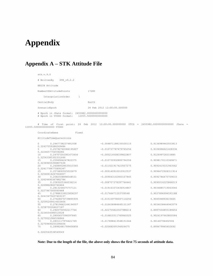
84
Appendix
Appendix A – STK Attitude File
stk.v.9.0
# WrittenBy STK_v9.2.2
BEGIN Attitude
NumberOfAttitudePoints 17280
InterpolationOrder 1
CentralBody Earth
ScenarioEpoch 24 Feb 2012 12:00:00.000000
# Epoch in JDate format: 2455982.00000000000000
# Epoch in YYDDD format: 12055.50000000000000
# Time of first point: 24 Feb 2012 12:00:00.000000000 UTCG = 2455982.00000000000000 JDate =
12055.50000000000000 YYDDD
CoordinateAxes Fixed
AttitudeTimeQuaternions
0 0.2447738237481938 -0.004871188155530115 0.9136989463553813
0.32437059386249484
5 0.25792760384195607 -0.010737787479765256 0.9106996621428336
0.3224657756558286
10 0.24707250381473456 -0.005214508339822807 0.912699728315885
0.32543385302331646
15 0.2594964247822375 -0.010730932800794356 0.9098170110349671
0.32369655394807634
20 0.26089528035610365 -0.011021917423507275 0.9092419331943562
0.32417784770895347
25 0.2576893525022879 -0.009140910010912537 0.9096672928311914
0.32560414267066007
30 0.2582508898548531 -0.009043102900107845 0.9092786470709033
0.32624690367882786
35 0.2583025366036214 -0.008707378397764441 0.9090016225866019
0.3269862860740464
40 0.2813244675757121 -0.019163372436914867 0.9034885719063046
0.3227967000060448
45 0.27888318525858297 -0.01766471203709548 0.9037896994593188
0.32415475637403157
50 0.27428676739895935 -0.015159790047116256 0.904594893615665
0.32595249414603406
55 0.27819662144194557 -0.016638984645131187 0.9034038464943579
0.3258700264637187
60 0.2920750502217764 -0.022755822567988214 0.8997504855189654
0.3234554086510028
65 0.2800457098397845 -0.016810311760860525 0.9024197663800584
0.3270021086558846
70 0.2831117976421769 -0.017898413548151044 0.90140794402506
0.32709490255396656
75 0.28982681789406856 -0.02068269194926675 0.899479945402692
0.3263563538549549
Note: Due to the length of the file, the above only shows the first 75 seconds of attitude data.
85
Appendix B – Languages and APIs
MATLAB
MATLAB is a high level language created by MathWorks® to be used by Engineers and Scientists. It is
created with an interactive environment, and is designed to easily analyze data, create models and
applications. It has many inbuilt mathematical functions for faster development time. It also has the
ability to perform calculations on vectors and matrices as part of its basic functionality.
Java
Java is a programming language designed as an object-oriented programming language that is based on
created classes to perform all the functions required. It was created by James Gosling and is currently
being maintained by the Oracle Corporation.
STK Components API
“STK Components is a collection of development libraries available in native
Java and .NET and built on industry-proven, fundamental and validated STK
algorithms. Using STK Components, you can deploy technology across the
enterprise or deliver it to your operational programs rapidly and affordably.
Use the key architectural elements of STK Components to build applications
that are:
Platform independent (pure .NET or Java libraries)
Thread safe and multithreaded
Highly scalable
Suitable for thick-client, thin-client or server deployment [66]”
Database
A database is a program created to store and retrieve data. This is done by issuing commands using a
querying language. One such database is the Oracle database which uses the SQL query language to store
and retrieve data. There are also other types of databases which are called NoSQL databases, which do
not use SQL to query – such examples are MongoDB and Counchbase.
Appendix C – Mission Operations Controllers
Spacecraft Controller: The Spacecraft Controller (SC), sometimes called a spacecraft
analyst, is a lead shift console position that directly interacts with the spacecraft and the
ground network during real-time supports. The SC performs the pre-pass briefing, may
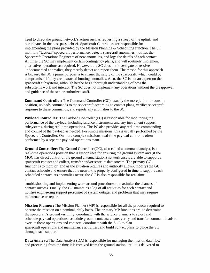
86
need to direct the ground network’s action such as requesting a sweep of the uplink, and
participates in the post-pass debrief. Spacecraft Controllers are responsible for
implementing the plans provided by the Mission Planning & Scheduling function. The SC
monitors “tactical” spacecraft performance, detects spacecraft anomalies, notifies the
Spacecraft Operations Engineers of new anomalies, and logs the details of each contact.
At times the SC may implement certain contingency plans, and will routinely implement
alternative operations as required. However, the SC does not investigate or resolve
undocumented anomalies, they merely detect and report them. The reason for this approach
is because the SC’s prime purpose is to ensure the safety of the spacecraft, which could be
compromised if they are distracted hunting anomalies. Also, the SC is not an expert on the
spacecraft subsystems, although he/she has a thorough understanding of how the
subsystems work and interact. The SC does not implement any operations without the preapproval
and guidance of the senior authorized staff.
Command Controller: The Command Controller (CC), usually the more junior on-console
position, uploads commands to the spacecraft according to contact plans, verifies spacecraft
response to these commands, and reports any anomalies to the SC.
Payload Controller: The Payload Controller (PC) is responsible for monitoring the
performance of the payload, including science instruments and any instrument support
subsystems, during real-time operations. The PC also provides any real-time commanding
and control of the payload as needed. For simple missions, this is usually performed by the
Spacecraft Controller. On more complex missions, real-time payload control is often
performed by a separate payload operations team.
Ground Controller: The Ground Controller (GC), also called a command analyst, is a
real-time operations position that is responsible for ensuring the ground system and (if the
MOC has direct control of the ground antenna station) network assets are able to support a
spacecraft contact and collect, transfer and/or store its data stream. The primary GC
function is to monitor (and as the situation requires and authority allows, modify) the GC
contact schedule and ensure that the network is properly configured in time to support each
scheduled contact. As anomalies occur, the GC is also responsible for real-time
7
troubleshooting and implementing work around procedures to maximize the chances of
contact success. Finally, the GC maintains a log of all activities for each contact and
notifies engineering support personnel of system outages and problems that may require
maintenance or repair.
Mission Planner: The Mission Planner (MP) is responsible for all the products required to
operate the mission on a nominal, daily basis. The primary MP functions are: to determine
the spacecraft’s ground visibility; coordinate with the science planners to select and
schedule payload operations; schedule ground contacts; create, verify and transfer command loads to
execute these operations and contacts; coordinate with the SOE to plan
spacecraft operations and maintenance activities; and build contact plans to guide the SC
through each support.
Data Analyst: The Data Analyst (DA) is responsible for managing the mission data flow
and processing from the time it is received from the ground station until it is delivered to
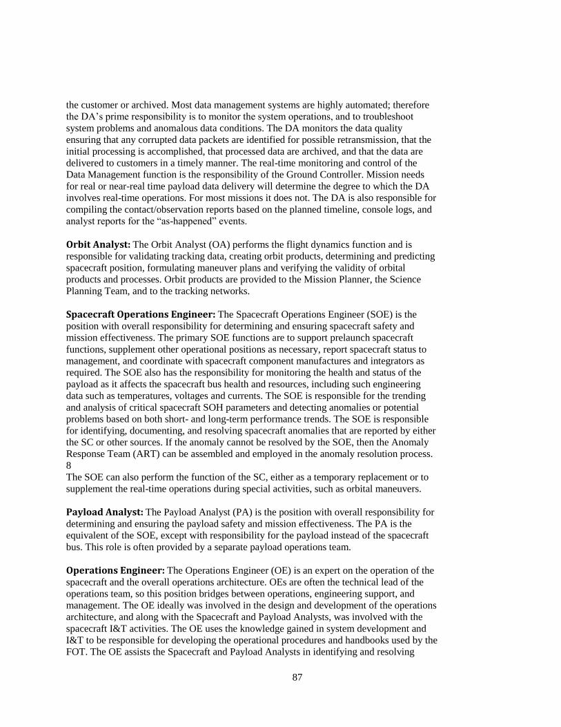
87
the customer or archived. Most data management systems are highly automated; therefore
the DA’s prime responsibility is to monitor the system operations, and to troubleshoot
system problems and anomalous data conditions. The DA monitors the data quality
ensuring that any corrupted data packets are identified for possible retransmission, that the
initial processing is accomplished, that processed data are archived, and that the data are
delivered to customers in a timely manner. The real-time monitoring and control of the
Data Management function is the responsibility of the Ground Controller. Mission needs
for real or near-real time payload data delivery will determine the degree to which the DA
involves real-time operations. For most missions it does not. The DA is also responsible for
compiling the contact/observation reports based on the planned timeline, console logs, and
analyst reports for the “as-happened” events.
Orbit Analyst: The Orbit Analyst (OA) performs the flight dynamics function and is
responsible for validating tracking data, creating orbit products, determining and predicting
spacecraft position, formulating maneuver plans and verifying the validity of orbital
products and processes. Orbit products are provided to the Mission Planner, the Science
Planning Team, and to the tracking networks.
Spacecraft Operations Engineer: The Spacecraft Operations Engineer (SOE) is the
position with overall responsibility for determining and ensuring spacecraft safety and
mission effectiveness. The primary SOE functions are to support prelaunch spacecraft
functions, supplement other operational positions as necessary, report spacecraft status to
management, and coordinate with spacecraft component manufactures and integrators as
required. The SOE also has the responsibility for monitoring the health and status of the
payload as it affects the spacecraft bus health and resources, including such engineering
data such as temperatures, voltages and currents. The SOE is responsible for the trending
and analysis of critical spacecraft SOH parameters and detecting anomalies or potential
problems based on both short- and long-term performance trends. The SOE is responsible
for identifying, documenting, and resolving spacecraft anomalies that are reported by either
the SC or other sources. If the anomaly cannot be resolved by the SOE, then the Anomaly
Response Team (ART) can be assembled and employed in the anomaly resolution process.
8
The SOE can also perform the function of the SC, either as a temporary replacement or to
supplement the real-time operations during special activities, such as orbital maneuvers.
Payload Analyst: The Payload Analyst (PA) is the position with overall responsibility for
determining and ensuring the payload safety and mission effectiveness. The PA is the
equivalent of the SOE, except with responsibility for the payload instead of the spacecraft
bus. This role is often provided by a separate payload operations team.
Operations Engineer: The Operations Engineer (OE) is an expert on the operation of the
spacecraft and the overall operations architecture. OEs are often the technical lead of the
operations team, so this position bridges between operations, engineering support, and
management. The OE ideally was involved in the design and development of the operations
architecture, and along with the Spacecraft and Payload Analysts, was involved with the
spacecraft I&T activities. The OE uses the knowledge gained in system development and
I&T to be responsible for developing the operational procedures and handbooks used by the
FOT. The OE assists the Spacecraft and Payload Analysts in identifying and resolving
88
anomalies and is responsible for developing, testing and implementing changes in
operational procedures, software, or hardware. They direct the efforts of the Software
Engineers in developing and testing approved patches or upgrades to both the ground and
flight software, based either on their own evaluations or from approved requests from the
remainder of the team. They also assist the Systems Engineer in developing and
implementing ground system process improvements, including automation.
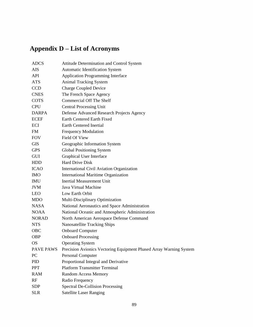
89
Appendix D – List of Acronyms
ADCS Attitude Determination and Control System
AIS Automatic Identification System
API Application Programming Interface
ATS Animal Tracking System
CCD Charge Coupled Device
CNES The French Space Agency
COTS Commercial Off The Shelf
CPU Central Processing Unit
DARPA Defense Advanced Research Projects Agency
ECEF Earth Centered Earth Fixed
ECI Earth Centered Inertial
FM Frequency Modulation
FOV Field Of View
GIS Geographic Information System
GPS Global Positioning System
GUI Graphical User Interface
HDD Hard Drive Disk
ICAO International Civil Aviation Organization
IMO International Maritime Organization
IMU Inertial Measurement Unit
JVM Java Virtual Machine
LEO Low Earth Orbit
MDO Multi-Disciplinary Optimization
NASA National Aeronautics and Space Administration
NOAA National Oceanic and Atmospheric Administration
NORAD North American Aerospace Defense Command
NTS Nanosatellite Tracking Ships
OBC Onboard Computer
OBP Onboard Processing
OS Operating System
PAVE PAWS Precision Avionics Vectoring Equipment Phased Array Warning System
PC Personal Computer
PID Proportional Integral and Derivative
PPT Platform Transmitter Terminal
RAM Random Access Memory
RF Radio Frequency
SDP Spectral De-Collision Processing
SLR Satellite Laser Ranging
90
SOTDMA Self-Organizing Time Division Multiple Access
SQL Structured Query Language
STK Satellite Toolkit
TCRS The International Reference System
TLE Two-Line Element
UHF Ultra-High Frequency
UK United Kingdom
UTC Coordinated Universal Time
UTIAS University of Toronto Institute for Aerospace Studies
VHF Very-High Frequency