A LAB TEXT BOOK ON

PHYSICS

By

Dr. Veena Bhatnagar

Department Of

Applied Sciences &

Humanities

Ansal Institute Of Technology

Huda Sector 55 , Gurgaon , Haryana

©Copyright Reserved

No part of this Lab Text Book may be repoduced , used , Stored without prior permission . First Edition : 2009

- 1 -

PREFACE

Physics forms a core subject which is taught to students of all disciplines of engineering in all the technical universities . The study of this subject is aimed at developing a through understanding of the basic concepts and principles of the Physics and their applications through the Lab work . Laboratory experimentation gives the clear understanding of the subject and opportunity to develop the techniques . For this laboratory manual is designed to meet the requirements of G.G.S.I.P ( IInd Semester ) students Some special features of this Lab manual are

• A brief description of the apparatus has been included along with relevant theoretical discussion of the experiment so that a student actually reads and understands it before starting the experiment . The system of recording the observations in a tabular form has been encouraged so that the various readings can be compared .

• The precautions have not only been given at the end of the experiment but also have been included in the instructions so that a student actually observes then even when he is performing the experiment .

This book is prescribed and helpful for Laboratory Experiments . Students are advised to study and perform the experiments according to the instructions during their Lab work . It is hoped that with all these & other features this book will prove very useful for the students .

- 2 -

Paper Code : ETPH-152 P C Paper : Applied Physics Lab – II 2 1 List of Experiments

1) To determine the value of e/m of electron by J.J.Thomson method .

2) To determine the low resistance by Carey Foster bridge after calibrating the bridge wire .

3) To determine the velocity of ultrasonic waves in a given liquid (say Kerosene oil )

4) To find the capacitance of a capacitor using flashing and quenching of a neon lamp.

5) To determine the temperature coefficient of resistance of platinum by means of Callendar and Griffith’s pattern bridge .

6) To determine the Hall Effect in Semiconductors and determine

(A) Hall Coefficient and Hall voltage (B) No. of charge carriers / unit volume (C) Hall mobility and Hall angle .

7) To find the co-efficient of thermal conductivity of a bad conductor by Lee’s method .

8) To determine the capacitance of a capacitor by discharging it through Voltmeter .

9) Find the internal resistance of leclanche cell using a potentiometer.

10) To draw the V-I characteristics of a forward and reverse bias junction diode and

to draw the load line.

11) To find the value of Plank’s constant and photo-electric work function .

Note : Atleast 8 experiments must be carried out . Proper error – analysis must be carried out with all the experiments .

- 3 -

Paper Code : ETPH-152 P C Paper : Applied Physics Lab – II 2 1

NAME OF EXPERIMENTS

EXPERIMENTS IN PART - I PAGE NUMBERS

1) To determine the value of e/m of electron by J.J.Thomson method . 5-to-12

2) To determine the low resistance by Carey Foster bridge after calibrating the bridge wire . 13-to-17

3) To determine the velocity of ultrasonic waves in a given liquid ( say Kerosene oil ) 18-to-22

4) To find the capacitance of a capacitor using flashing and quenching of a neon lamp. 23-to-28

5) To determine the temperature coefficient of resistance of platinum by means of Callendar and Griffith’s pattern bridge . 29-to-33 6) To determine the Hall Effect in Semiconductors and determine a. Hall Coefficient and Hall voltage b. No. of charge carriers / unit volume c. Hall mobility and Hall angle . 34-to-41

EXPERIMENTS IN PART - II PAGE NUMBERS

7) To find the co-efficient of thermal conductivity of a bad conductor by Lee’s method . 1-to-5

8) To determine the capacitance of a capacitor by discharging it through Voltmeter . 6-to-9 9) Find the internal resistance of leclanche cell using a potentiometer. 10-to-13

10) To draw the V-I characteristics of a forward and reverse bias junction diode and to draw the load line. 14-to-20 11) To find the value of Plank’s constant and photo-electric work function . 21-to-27

Note : Atleast 8 experiments must be carried out . Proper error – analysis must be carried out with all the experiments .

- 4 -

EXPERIMENT 1

AIM :- To determine the value of e/m for an electron by Thomson’s method using bar magnets.

APPRATUS USED :- A cathode ray tube fitted on a wooden stand provided with two arms perpendicular to the axis of the tube and having scales with zero at the point where the central line of the arms cuts the axis of the tube; a power supply unit capable of giving the accelerating D.c. voltage for the cathode ray tube and the deflecting D.C. voltage for the electric field through a reversing key with suitable voltmeters, two bar magnets, a compass box, a compass needle, etc.

THEORY :- The value of e/m can be determined by the method originally used by Prof. J.J. Thomson

The apparatus consists of a cathode ray tube which has three essential parts. (i) The electron gun. This part consist of the cathode K and the anode A. It produces, accelerated and focuses the electrons into a fine beam so as to produce a small bright spot on the fluorescent screen S.

(ii) The screen. The screen S is coated with some fluorescent material like zinc sulphide etc. so that a greenish blue spot of light is observed where the electron beam impinges upon the screen. A transparent mm graph is attached to the screen to note the exact position of the fluorescent spot.

Measurement of e/m and Electronic Charge

(iii) The electric and magnetic deflecting system. Two plates P and Q are fitted in the tube symmetrically on either side of the electron beam so that an electric field perpendicular to the plane of the paper can be applied between them.

Figure 1.

A magnetic field can also be applied at the same place in a direction perpendicular to the direction of the electric field i.e. in the plane of the paper. Thus the deflection of the cathode rays due to the electric as well as the magnetic, field takes place in a direction perpendicular to the plane of the paper.

To apply the magnetic field the cathode ray tube is fitted on a wooden stand provided with two arms, one on either side perpendicular to the direction of the electron beam. A

- 5 -

scale is marked on each arm which gives the distance from the axis of the cathode ray tube. When two bar magnets are placed with their lengths parallel to the arms with their opposite poles towards the cathode ray tube, these produce a uniform magnetic field exactly at the same place where an electric field produced when a potential difference is applied between the plates P and Q.

Figure 2

Theory. Let E be intensity of the electric field applied between the plates P and Q in a direction perpendicular to the plane of the paper then the force acting on the electron of charge e

= Ee

This force acts at right angles to the direction of motion of the electron. The electron, therefore, moves along a circular path within the electric field and on leaving the field flies off tangentially to the path meeting the screen at M1 or M2 depending up to the direction of the electric field as shown in Fig. 3. (a) and (b). When a magnetic field B is applied in the plane of the paper perpendicular to the direction of the beam as show in in figure 4. (a) then according to Fleming’s left hand rule the beam is deflected upward cut of the paper in a direction perpendicular to both, the direction of motion of the electron and that of the field.

Figure 3

- 6 -

When the magnetic field is applied as shown in Figure 4. (b) the electron beam is deflected downward into the paper. If v is the velocity of the electrons in the beam, then magnitude of the force acting on each electron = B e.v. As this force also acts at right angles to the direction of motion of the electron, the electron moves along a circular path in the magnetic field and on leaving the field flies off tangentially meeting the screen at M1 or M2 as explained above.

Figure - 4

If r is the radius of the circular path along which the electron moves in the magnetic field, then

B e v = r

mv 2

Or rBv

me= ……(i)

To find the velocity of electron v: To find the value of V, one of the fields say the magnetic field is first applied. The spot of light moves from its initial position to the position say M1. The electric field is now applied simultaneously so as to produce deflection of the electron beam in the opposite direction. The value of the electric field is so adjusted that the spot of light comes back to its initial position. In such a case the forces acting on the electron due top the electric and magnetic fields are equal and opposite.

∴ Ee = B e v

Or v = BE

Substituting in (i), we have

2rBE

me= ………(ii)

To find the radius r of circular path. To find the value of r, the radius of the circular path in the magnetic field, note the position f the luminous spot on the screen when no field is applied and again when a field B is applied. Let the deflection of the spot be y = LM2 as shown. The circular path of the beam OR in the magnetic field is as shown in Figure 2. The beam leaves the magnetic field at R tangenially to the path and meets the screen at M2 so that M2 R produced meets OX in T. Draw OC and RC perpendiculars to OL and RM2 respectively meeting at C, then C is the centre of the circular are OR and OC = CR radius of the circle = r

Now ∠OCR = ∠LT M2 = θ

- 7 -

∴ tan θ = OCOX

LTLM

=2

∴ r = OC = 2LMOXLT ×

Now OX is very nearly equal to the length of the region in which the magnetic field is applied. This is also equal to the length of the region in which the electric field is applied. I.e. the length of the plates P and Q. Let it be = l (This is generally given by the makers).

Figure 5

Measurement of e/m and Electronic Charge

LT is the distance of the centre of the screen from the centre of the region of the magnetic field (or electric field). Let is be = L

∴ r = yLl

Substituting in (ii), we have

2LlByE

me= …… (iii)

The electric field E = dV where V is the potential difference applied between the

plates P and Q and d the distance between the plates (d is also given by the markers). Substituting in (iii), we have

2LldByV

me=

When V is in volts, B in Tesla and y, L, I, and d in meters e/m is in Coulomb/kg.

PROCEDURE :

- 8 -

(1) Draw the North South line using a compass needle. Also draw the East-West line. Place the cathode ray tube fitted in the wooden frame with its axis along the North South line so that the arms of the frame lie along the East West line.

(2) Connect the cathode ray tube to the power supply unit. Switch on the current and wait till a luminous bright spot appears on the screen. Adjust the brightness and focus controls so as to get a sharp bright point spot in the middle of the screen. Note the initial position of the spot on the scale fitted on the screen.

(3) Now apply a suitable deflecting voltage so that the luminous spot is deflected by about 0.5 to 1.0 cm. Note the deflecting voltage V and the position of the spot. Measure the distance through which the spot has moved and let it by y.

(4) Place the bar magnets symmetrically on either side of the cathode ray tube along the arms of the wooden stand on which the tube is fitted such that their opposite poles face each other and their common axis is exactly at right angles to the axis of the cathode ray tube. Adjust the polarity as well as the distance of the magnets so that the luminous spot comes back to its initial position. When the adjustment is perfect note the distance of the poles of the magnets on the side nearer to the cathode ray tube. Let the distances be r1 and r2.

(5) Remove the bar magnet, switch off the electric field applied to the deflecting plates and again note the initial position of the luminous spot. Reverse the polarity of the potential difference applied to the electric deflecting plates with the help of the reversing switch fitted in the power supply unit thereby reversing the electric field. Again note the final position of the luminous spot and calculate y.

Again place the bar magnets on the arms of the wooden stand as in the previous step and adjust their polarity as well as the distance so comes back to its initial position. When the adjustment is perfect again note the distances of the poles of the magnets on the side nearer to the cathode ray tube. Let the distances be r’1 and r’2. Switch off the power supply.

(6) To find the value of the magnetic field B, carefully remove the magnets and the cathode ray tube from the wooden stand. Place the compass box (of a deflection magnetometer or tangent galvanometer) such that its centre lies exactly on the point where the common axis of the bar magnets and the axis of the cathode ray tube intersect. Rotate the compass box about its vertical axis so that the pointer lies along the 0-0 line.

Place the magnets exactly in the same positions as in step 4 at distances r1 and r2. This produces a deflection in the magnetometer compass box and the two ends of the pointer give the deflection. Let the readings be θ1 and θ2.

Now place the magnets exactly, in the same positions as in step 5 at distances r’1 and r’2 and again note the deflections θ’1 and θ’2 from the two ends of the pointer of the compass box. The mean of these four deflection θ1, θ2, θ’2 and θ’2 gives the mean deflection θ. If BH is the horizontal component of earth’s magnetic field, then

B = BH tan θ

- 9 -

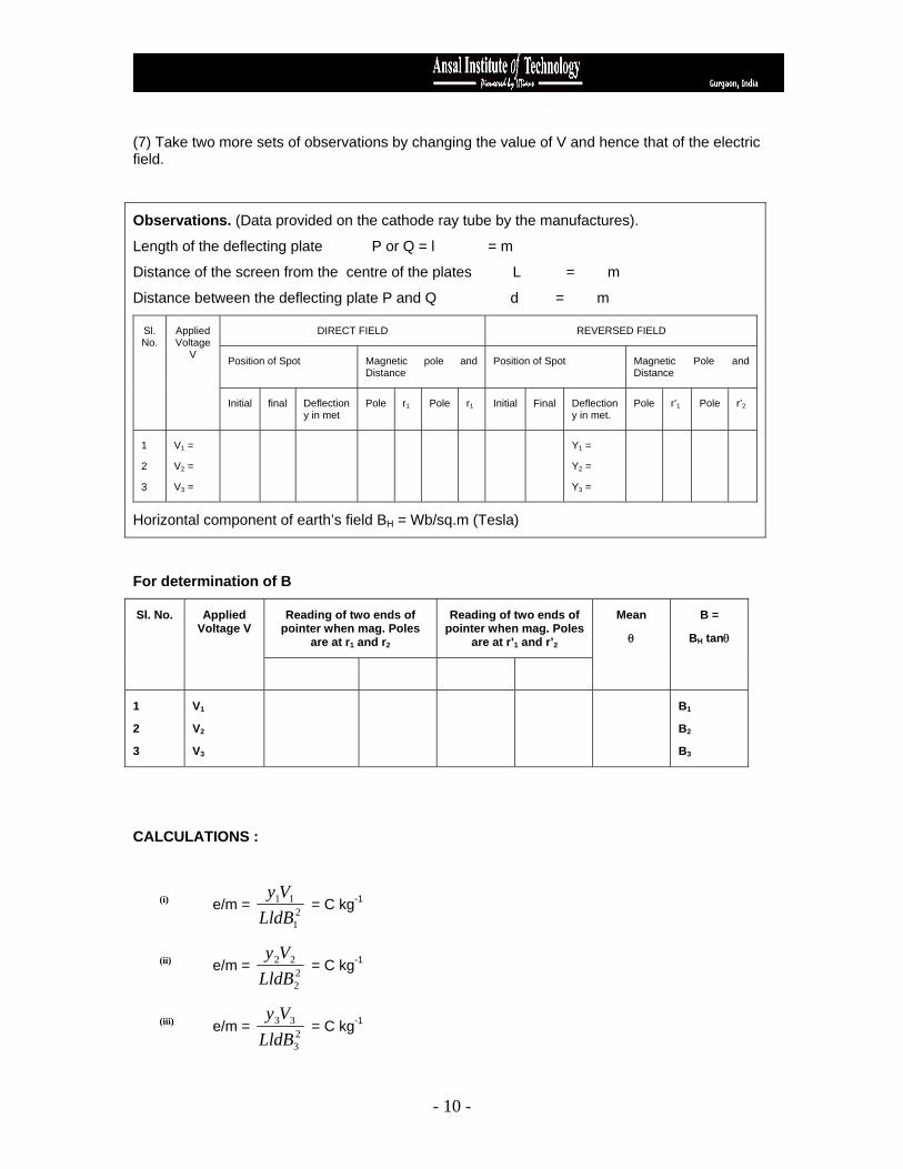
(7) Take two more sets of observations by changing the value of V and hence that of the electric field.

Observations. (Data provided on the cathode ray tube by the manufactures).

Length of the deflecting plate P or Q = l = m

Distance of the screen from the centre of the plates L = m

Distance between the deflecting plate P and Q d = m

DIRECT FIELD REVERSED FIELD

Position of Spot Magnetic pole and Distance

Position of Spot Magnetic Pole and Distance

Sl. No.

Applied Voltage

V

Initial final Deflection y in met

Pole r1 Pole r1 Initial Final Deflection y in met.

Pole r’1 Pole r’2

1

2

3

V1 =

V2 =

V3 =

Y1 =

Y2 =

Y3 =

Horizontal component of earth’s field BH = Wb/sq.m (Tesla)

For determination of B

Reading of two ends of pointer when mag. Poles

are at r1 and r2

Reading of two ends of pointer when mag. Poles

are at r’1 and r’2

Sl. No. Applied Voltage V

Mean

θ

B =

BBH tanθ

1

2

3

V1

V2

V3

BB1

BB2

BB3

CALCULATIONS :

(i) e/m = 21

11

LldBVy

= C kg-1

(ii) e/m = 22

22

LldBVy

= C kg-1

(iii) e/m = 23

33

LldBVy

= C kg-1

- 10 -

Measurement of e/m and Electronic charge

(iii) e/m = 23

33

LldBVy

= C kg-1

Mean e/m = Ckg-1

PRECAUTIONS :

(1) The cathode ray tube must be set in the north south direction.

(2) The luminous spot on the screen should be sharp, bright and in the middle.

(3) The deflecting voltage must produce a deflection of the order of 0.5 to 1.0 cm.

(4) The axis of the bar magnets and the axis of the cathode ray tube must be exactly at right angles and in a horizontal plane.

(5) The deflecting voltage must be reversed to produce the deflection of the spot of light in the opposite direction and the magnetic field must also be reversed to bring it back to initial position.

(6) The cathode ray tube must be handled carefully.

- 11 -

SPACE FOR STUDENTS WORK AREA

- 12 -

EXPERIMENT 2

AIM : To find the low resistance by Carey Foster bridge after calibrating the bridge wire.

APPRATUS USED : Carey-Foster bridge, two equal resistance, thick copper strips, a fractional resistance box (or standard fractional resistance coils), a cell, connecting wires, a sensitive galvanometer, a jockey and a key. THEORY : The arrangement of Carey-Foster bridge is similar to Wheatstone bridge. As shown in Figure (…), P and Q are the two ratio arms, X along with the resistance of wire aD and Y along with the resistance of the wire bD form the other two arms.

If ρ is the resistance per cm of the wire, λl and λ2 the end resistances at a and b respectively, and a balance point is obtained at D, where aD = l1, then

( ) 22

11

100 λρλρ+−+

++=

lYlX

QP

…..(i)

If now, X and Y are interchanged and the balance point is obtained at D’ as show in Figure 1 such that a D’ is equal to l2, then

( ) 21

12

100 λρλρ+−+

++=

lXlY

QP

……(ii)

Comparing (i) and (ii) and adding one to both sides, we have

( ) 21

21

100100

λρλλρ

+−+++++

lYYX

= ( ) 22

21

100100

λρλλρ

+−+++++

lXYX

Or ( ) 21100 λρ +−+ lY = ( ) 22100 λρ +−+ lX

Or ( )ρ21 llXY −=−

Or ( )ρ21 llYX −−=

Thus, the difference between the two resistances is equal to the resistance of the bridge wire between the two balance points. Further the above relation is free from the end correction of the total length of the bridge wire.

Figure 1

- 13 -

PROCEDURE :

(1) Connections.

(i) Draw a diagram showing the scheme of connection as in Figure 2. Mark the gaps 1, 2, 3 and 4 on the bridge.

(ii) Clean the ends of the connecting wires and the thick copper strip with a sand paper.

(iii) Connect the two equal resistance P and Q in the inner gaps 2 are 3. If P and Q are two resistance boxes, take out 5 ohm plug from either and make all other plugs tight. Connect the thick copper strip X in the gap 1 and th fractional resistance box by means of thick copper rods in the gap 4. Connect one terminal of the galvanometer to the central terminal B and the other to a jockey J. Connect the cell through a key between the points A and C. Show the connection to the instructor before passing the current.

(2) To test the connections. Make the plugs of the fractional resistance box tight by giving to each plugs a slight twist. Put in the key K and touch the jockey on the wire at the end a. Note the direction of deflection. Now touch the jockey at the end b. If the direction of deflection is reversed the connections are correct.

(3) To find ρ, the resistance per cm of the wire. (i) Without taking out any plug from the fractional resistance box, adjust the position of the jockey to obtain a balance point and note the reading. Take out the key K. Interchange X and Y, put in the key K and obtain the balance point a gain. Note the reading.

The difference in the two positions gives us the resistance of the lead wires connected in the fractional resistance box (Y) and the resistance of the plugs, brass blocks etc. This shift is known as the correction and must be subtracted from the shift obtained in the subsequent readings to the correct shift. Let this be denoted by δl.

(ii) Take out 0.1 omh plug from the fractional resistance box YU and after putting the K obtain the balance point. Note the reading and interchange X and Y. Again obtain the balance point and no it.

(iii) Repeat the observation with the values of Y equal to 0.2, 0.3, 0.4 and 0.5 ohm etc.

To find the low resistance. Disconnect the copper strip and connect either the given low resistance in the form of a small piece of wire W soldered to two thick copper strips S1 and S2 as shown in Figure 2 or the two turns coil of the tangent galvanometer in its place by pieces of short thick copper wires. Keeping the resistance in the fractional resistance box zero, find the balance point. Interchange the tangent galvanometer and the fractional resistance box and find the balance point again. Similarly repeat the observation by taking out 0.1, 0.2, 0.3, 0.4 and 0.5 ohm resistance from the fractional resistance box.

- 14 -

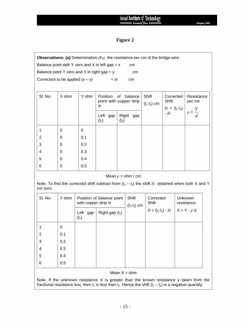
Figure 2

Observations: (a) Determination of ρ, the resistance per cm of the bridge wire.

Balance point with Y zero and X in left gap = x cm

Balance point Y zero and X in right gap = y cm

Correction to be applied (x – y) = δl cm

Position of balance point with copper strip in

Sl. No. X ohm Y ohm

Left gap (l1)

Right gap (l2)

Shift

(l1-l2) cm

Corrected Shift

D = (l1-l2) - δl

Resistance per cm

ρ = dY

1

2

3

4

5

6

0

0

0

0

0

0

0

0.1

0.2

0.3

0.4

0.5

Mean ρ = ohm / cm

Note. To find the corrected shift subtract from (l1 – l2) the shift δl obtained when both X and Y zre zero.

Position of balance point with copper strip in

Sl. No. Y ohm

Left gap (l1)

Right gap (l2)

Shift

(l1-l2) cm

Corrected Shift

D = (l1-l2) - δl

Unknown resistance

X = Y - ρ d

1

2

3

4

5

6

0

0.1

0.2

0.3

0.4

0.5

Mean X = ohm

Note. If the unknown resistance X is greater than the known resistance y taken from the fractional resistance box, then l1 is less than l2. Hence the shift (l1 – l2) is a negative quantity.

- 15 -

If X is less than Y, l1 is greater than l2 and hence the shift (l1 – l2) is positive.

Precautions.

1. The ends of connecting wires, thick copper strip and the leads for the resistance box should be properly cleaned.

2. The unknown low resistance should be connected to the bridge by thick copper leads.

3. The plugs of the fractional resistance box should be tight.

4. The batter key should be taken out while interchanging X and Y to avoid heating of the bridge wire.

5. In order that the bridge may be sensitive, the resistances of the four arms should be nearly of the same order. This is why P and Q should not be very large.

6. The jockey should be touched gently and should not be kept pressed on to the wire while shifting it from one point to the other.

7. The difference between X and Y should not be more than the resistance of the bridge wire.

- 16 -

SPACE FOR STUDENTS WORK AREA

- 17 -

EXPERIMENT 3 AIM : To find the velocity of ultrasonic waves in a given liquid (say kerosene oil).

APPARATUS USED : A glass cell, kerosene oil, quartz crystal slab fitted with two leads, ultrasonic spectrometer, convex lens, sodium lamp, radio frequency oscillator with frequency measuring meter ,spirit level etc.

THEORY : We can find the velocity of sound in a liquid (say kerosene oil) using ultrasonic.

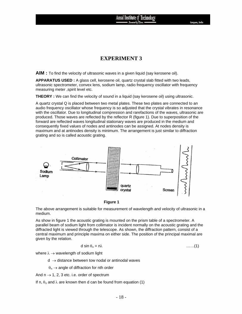
A quartz crystal Q is placed between two metal plates. These two plates are connected to an audio frequency oscillator whose frequency is so adjusted that the crystal vibrates in resonance with the oscillator. Due to longitudinal compression and rarefactions of the waves, ultrasonic are produced. Those waves are reflected by the reflector R (figure 1). Due to superposition of the forward are reflected waves longitudinal stationary waves are produced in the medium and consequently fixed values of nodes and antinodes can be assigned. At nodes density is maximum and at antinodes density is minimum. The arrangement is just similar to diffraction grating and so is called acoustic grating.

Figure 1

The above arrangement is suitable for measurement of wavelength and velocity of ultrasonic in a medium.

As show in figure 1 the acoustic grating is mounted on the prism table of a spectrometer. A parallel beam of sodium light from collimator is incident normally on the acoustic grating and the diffracted light is viewed through the telescope. As shown, the diffraction pattern, consist of a central maximum and principle maxima on either side. The position of the principal maximal are given by the relation.

d sin θn = nλ ……(1)

where λ → wavelength of sodium light

d → distance between tow nodal or antinodal waves

θn → angle of diffraction for nth order

And n → 1, 2, 3 etc. i.e. order of spectrum

If n, θn and λ are known then d can be found from equation (1)

- 18 -

If λm is the wavelength of ultrasonic through the medium, then

d = 2mλ

or λm = 2 d

If the resonant frequency of the piezoelectric oscillator is N, the velocity of ultrasonic waves is given by

v = Nλm

= 2 Nd

The above method is useful for determination of velocity of ultrasonic waves through liquids and gases at various temperatures.

λm = ndDnλ

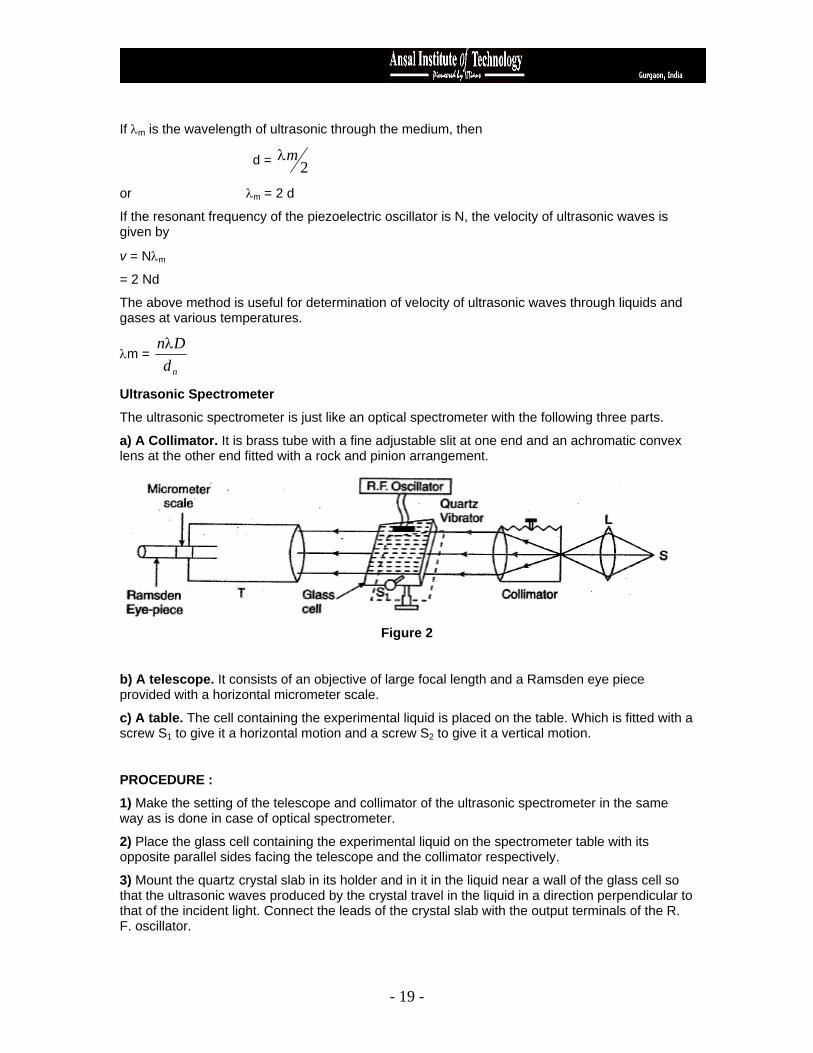
Ultrasonic Spectrometer

The ultrasonic spectrometer is just like an optical spectrometer with the following three parts.

a) A Collimator. It is brass tube with a fine adjustable slit at one end and an achromatic convex lens at the other end fitted with a rock and pinion arrangement.

Figure 2

b) A telescope. It consists of an objective of large focal length and a Ramsden eye piece provided with a horizontal micrometer scale.

c) A table. The cell containing the experimental liquid is placed on the table. Which is fitted with a screw S1 to give it a horizontal motion and a screw S2 to give it a vertical motion.

PROCEDURE :

1) Make the setting of the telescope and collimator of the ultrasonic spectrometer in the same way as is done in case of optical spectrometer.

2) Place the glass cell containing the experimental liquid on the spectrometer table with its opposite parallel sides facing the telescope and the collimator respectively.

3) Mount the quartz crystal slab in its holder and in it in the liquid near a wall of the glass cell so that the ultrasonic waves produced by the crystal travel in the liquid in a direction perpendicular to that of the incident light. Connect the leads of the crystal slab with the output terminals of the R. F. oscillator.

- 19 -

4) Put the quartz crystal in its holder and place it in the liquid near a wall of the glass cell so that the ultrasonic produced by the crystal move perpendicularly to the direction of incident light. Make the connection of R.F. oscillator with the leads of crystal slab.

5) Focus the light from sodium lamp on the slit of collimator. Look through the telescope eye-piece and get a wall defined image of the slit at the centre of the micrometer scale fitted in the ey-piece of the telescope.

6) Switch on the R.F. oscillator so that the ultrasonic waves are produced in the liquid. Make the adjustment of frequency from the oscillator so that it becomes equal to the natural frequency of the crystal slab and resonance takes place and diffraction images of the slit will be visible through the telescope. An enlarged view of diffraction pattern is show in figure 3. Note down the frequency of the R.F. oscillator and keep it constant throughout the experiment.

Figure 3

7) Note down the distance of various order diffraction image on both sides of the central zero using the micrometer scale of the eye piece of telescope.

8) Also measure the distance D between the objective lens of telescope and the crosswire (micrometer scale). It will correspond to the focal length of the objective lens and is normally provided by the manufacture of the instrument.

OBSERVATIONS : Wavelength of Sodium light λ = 5893 x 10-10 m

Room temperature = ° C

Distance D = cm

Frequency of the oscillator used v = Hz

Least count of the micrometer scale = …… mm

Position of diffracted image in cm

Left of central image Right of central image

S. No.

Order of diffraction maxima

N Main scale

Vernier scale

Total x Main scale

Vernier scale

Total y

2yxdn

−= cm

ndn

- 20 -

1

2

:

:

10

Mean value of n

dn = cm = m

Wavelength of ultrasonic waves

mdDD

dn

nnn =

λ=λ=λ

Velocity of ultrasonic waves = vλ = ……. ms-1

PRECAUTIONS

1. The diffraction pattern should be sharp and narrow.

2. The glass cell should be thoroughly cleaned and filled with the liquid.

3. The crystal slab should be set in such a way that the ultrasonic waves produced by it travel be kept constant during the experiment.

5. The crystal slab should be immersed completely in the liquid and should touch neither the bottom nor the side of the walls.

- 21 -

SPACE FOR STUDENTS WORK AREA

- 22 -

EXPERIMENT 4

AIM : To find the capacitance of a capacitor using flashing and quenching of a neon lamp.

APPRATUS USED : A capacitor of unknown capacitance, capacitors of known capacitance (say 0.1, 0.2, 0.5 µF), a neon flashing lamp, a resistance of about 1 meg ohm, regulated D.C. power supply capable of giving upto 150 volts and 5 keys.

Figure (1)

Note : Neon lamps intended to be connected direct to H.T. have a ballast resistor of about 2000 ohm sealed into the cap to limit the current. This must be removed for this experiment. Alternatively small neon flash bulbs without any resistor sealed in are available from radio dealers.

THEORY :

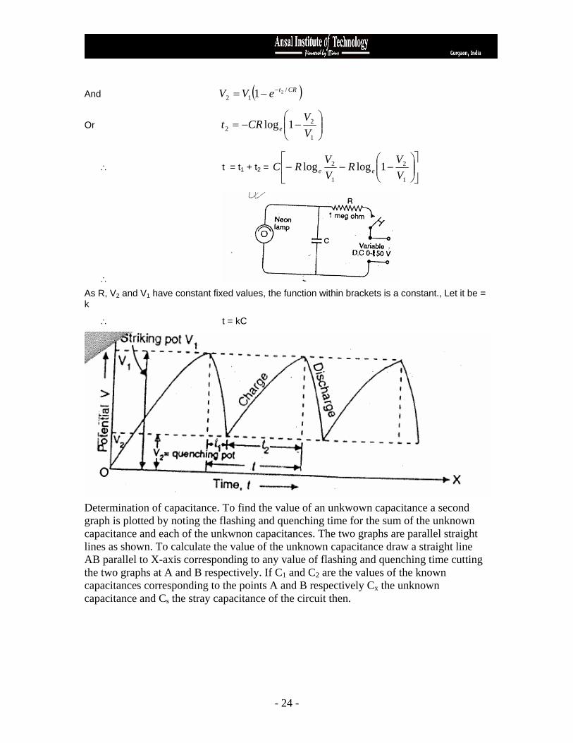
Flashing and quenching of a neon bulb. A neon bulb is placed in parallel with a capacitor and connected to D.C. supply which can be continuously increased from 0 to 150 volt through a high resistance of about 1 meg. Ohm. The voltage is slowly increased to a value say V1 when the lamp flashes and begins to glow. As soon as the neon lamp flashes, it becomes conducting and the capacitor begins to discharge through it. It continues to do so until the extinction (or quenching) potential V2 is reached when the neon lamp ceases to glow and stops conducting. The capacitor then again beings to charge till the flashing potential V1 is reached when again the lamp flashes and begins to glow. The process is repeated, During the time the capacitor is charging the neon lamp does not glow. In other words, the total time t between two consecutive flashes is equal to the time taken by the voltage first to fall from the flashing potential V1 to quenching potential V2 (discharge) and then to rise from V2 to V1 (charging). This flashing and quenching time can be determined by noting the time taken by the lamp to produce say 20 consecutive flashes and quenches.

If t1 is the time taken by the capacitor voltage to fall from V1 to V2 and t2 is the time taken by the voltage to rise from V2 to V1, then

CRteVV /12

1−=

Or 1

21 log

VVCRt e−=

- 23 -

And ( )CRteVV /

1221 −−=

Or ⎟⎟⎠

⎞⎜⎜⎝

⎛−−=

1

22 1log

VVCRt e

∴ t = t1 + t2 = ⎥⎦

⎤⎢⎣

⎡⎟⎟⎠

⎞⎜⎜⎝

⎛−−−

1

2

1

2 1loglogVVR

VVRC ee

∴ As R, V2 and V1 have constant fixed values, the function within brackets is a constant., Let it be = k

∴ t = kC

Determination of capacitance. To find the value of an unkwown capacitance a second graph is plotted by noting the flashing and quenching time for the sum of the unknown capacitance and each of the unkwnon capacitances. The two graphs are parallel straight lines as shown. To calculate the value of the unknown capacitance draw a straight line AB parallel to X-axis corresponding to any value of flashing and quenching time cutting the two graphs at A and B respectively. If C1 and C2 are the values of the known capacitances corresponding to the points A and B respectively Cx the unknown capacitance and Cs the stray capacitance of the circuit then.

- 24 -

Total capacitance corresponding to point A

= Cs + C1 + Cx

And total capacitance corresponding to point B

= Cx + C2

Since the flashing and quenching time for both is the same

K(Cs + C1 + Cx) = k (Cx + C2)

Or Cx = C2 – C1

PROCEDURE :

1. Draw a diagram showing the scheme of connections as in Figure (1) and make connections accordingly.

2. Connect the capacitance C1 in the circuit by putting in the key K1. Put in the key K and increase the power supply voltage slowly till the neon lamp just begins to flash. As it is connected in parallel.

Remove the key K to disconnect the power supply. Put in the key K4 so that the capacitors C1 and Cx (of unknown capacitance) are connected in parallel and total capacitance is equal to their sum C1 + Cx. Again put in the key K (see that the power supply voltage remains constant). Note the time of 20 flashes. Remove the keys K, K4 and K1.

3. Repeat the experiment with capacitors C2 alone and (C2 + Cx); C3 alone and (C3 + Cx). Now put in the keys K1 and K2 so that the total capacitance (C1 + C2) is in the circuit. Repeat the experiment with (C1 + C2) and then with [(C1 + C2)+Cx]. Similarly repeat the experiment with (C1 + C3) and [(C1 + C3)+Cx], (C1 + C2 + C3) and [(C1 + C2 + C3)+Cx]

- 25 -

OBSERVATION :

1

Sl.No.

2

Known

Capacitance

3

Time for 20

Flashes without Cx

4

Flashing and

Quenching time t

5

Time for 20

Flashes with Cx

6 Flashing and

Quenching time t

C1 =

C2 =

C3 =

C1 + C2 =

C1 + C3 =

C1 + C2 + C3

4. Plot two graphs (i) between values of capacitance in column 2 taken along X-axis and flashing and quenching time t in column 4 (without unknown capacitance) and (ii) between values of capacitance in column 2 and quenching and flashing time t in column 6 (with unknown capacitance) taken along the Y-axis. For three different values of flashing and quenching time draw three straight lines. Parallel to X-axis cutting the two graphs at A and B, C and D, and E and F respectively.

Figure (2)

- 26 -

The unknown capacitance

Cx = AB = CB – CB A

= CD = CD - CC

= EF = CF – CE

Mean Cx = µF

PRECAUTIONS

1. The voltage from the D.C. power supply should remain constant throughout the experiment.

2. The resistor sealed in the cap of the neon lamp should be removed before using it for the experiment, otherwise a bulb without resistor should be used.

- 27 -

SPACE FOR STUDENTS WORK AREA

- 28 -

EXPERIMENT 5

AIM: To determine the temperature coefficient of resistance of platinum by means of Callendar and Griffith’s pattern bridge.

APPARATUS : Platinum resistance thermometer, Callenar and Griffith’s pattern bridge, a Leclanche cell, a galvanometer, beaker (600 c.c. capacity), electric stove, a decimal-ohm dial box, a mercury thermometer and connection wires.

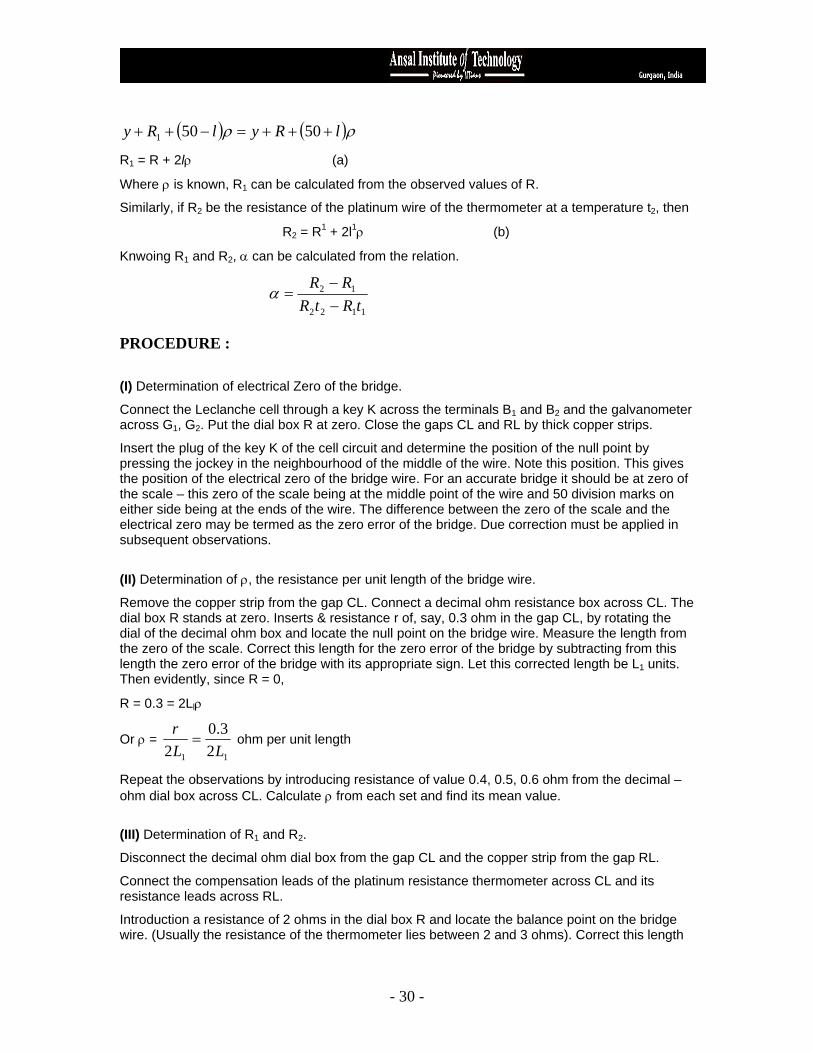
THEORY : Callendar and Griffith’s pattern bridge. For work at the undergraduate level such a piece of apparatus is manufactured. By Instrument & Chemicals Ltd. Ambala. The circuit diagram of the bridge is given in figure 1.

Figure 1

The ratio coils P and Q have equal resistance, so that the ratio is 1:1. CL and RL are the gaps for connecting the compensating and the resistance leads of the thermometer. R is a dial pattern resistance, each coil having a resistance of one ohm. In series with this is a stretched wire W, also of resistance one ohm. The scale for the reading of the length of the wire is graduated with zero in the middle and 50 division marks at either end. Thus the value ρ, the resistance per unit length of the bridge wire is 1/100 ohms per unit length. Suppose with connections as shown in the figure above, the null point is at a length l measured frm middle points of the wire. Let R1 be the required resistance of the platinum wire, say at room temperature t1 and R the resistance introduced in the dial box. Then

( )( )ρ

ρlRylRy

QP

−+++++

==50501

1

Where ρ is the resistance per unit length of the bridge wire and y is the resistance of the leads. From the above equation we have

- 29 -

( ) ( )ρρ lRylRy +++=−++ 50501

R1 = R + 2lρ (a)

Where ρ is known, R1 can be calculated from the observed values of R.

Similarly, if R2 be the resistance of the platinum wire of the thermometer at a temperature t2, then

R2 = R1 + 2l1ρ (b)

Knwoing R1 and R2, α can be calculated from the relation.

1122

12

tRtRRR

−−

=α

PROCEDURE : (I) Determination of electrical Zero of the bridge.

Connect the Leclanche cell through a key K across the terminals B1 and B2 and the galvanometer across G1, G2. Put the dial box R at zero. Close the gaps CL and RL by thick copper strips.

Insert the plug of the key K of the cell circuit and determine the position of the null point by pressing the jockey in the neighbourhood of the middle of the wire. Note this position. This gives the position of the electrical zero of the bridge wire. For an accurate bridge it should be at zero of the scale – this zero of the scale being at the middle point of the wire and 50 division marks on either side being at the ends of the wire. The difference between the zero of the scale and the electrical zero may be termed as the zero error of the bridge. Due correction must be applied in subsequent observations.

(II) Determination of ρ, the resistance per unit length of the bridge wire.

Remove the copper strip from the gap CL. Connect a decimal ohm resistance box across CL. The dial box R stands at zero. Inserts & resistance r of, say, 0.3 ohm in the gap CL, by rotating the dial of the decimal ohm box and locate the null point on the bridge wire. Measure the length from the zero of the scale. Correct this length for the zero error of the bridge by subtracting from this length the zero error of the bridge with its appropriate sign. Let this corrected length be L1 units. Then evidently, since R = 0,

R = 0.3 = 2Llρ

Or ρ = 11 23.0

2 LLr

= ohm per unit length

Repeat the observations by introducing resistance of value 0.4, 0.5, 0.6 ohm from the decimal – ohm dial box across CL. Calculate ρ from each set and find its mean value.

(III) Determination of R1 and R2.

Disconnect the decimal ohm dial box from the gap CL and the copper strip from the gap RL.

Connect the compensation leads of the platinum resistance thermometer across CL and its resistance leads across RL.

Introduction a resistance of 2 ohms in the dial box R and locate the balance point on the bridge wire. (Usually the resistance of the thermometer lies between 2 and 3 ohms). Correct this length

- 30 -

for the zero error of the bridge wire and knowing the values of R, L and ρ, calculate R1 from equation a.

By changing the value of R to 3 ohms, redetemine the value of R1. It may be noticed here that with R equal to 2 ohms, the balance point was on the positive side of the scale (i.e., on to the right of zero of the scale) whereas with R equal to three ohms, the balance point is obtained on the left hand side of the zero, i.e. on the negative side of the scale. In the latter case R1 will be calculated from the relation

R1 = R – 2lρ

Find the mean value of R1. Record the room temperature t1 °C. Thus the resistance R1 of the platinum coil is known at a temperature t1°C.

Next place the platinum resistance thermometer in a large beaker or container with water. Allow the water to boil by heating the container over an electric stove. Also put a mercury thermometer to record the temperature t2 of boiling water.

When water in the container has been boiling for about ten minutres or so, introduce a resistance of 3 ohms in the diall, box R and locate the new balance point on the b4ridge wire, which will now be again on the positive side of scale. Repeat this observation after every twominutes, and when the reading does not change it can be assumed that the platinum coil has attained the temperature t2 °C of boiling water, as recorded by the mercury thermometer. Note this length for the balance point and correct it for zero error. From a knowledge of the resistance R (-3 ohms), the corrected length l1 for balance and …. Calculate R2 from the equation (b)

Put R at 4 ohms and redetermine the value of R2. Compute the mean value of R2 from those two determinations. SOURCE OF ERROR AND PRECAUTIONS

1) The decimal ohm box should be preferably of dial pattern and should be connected by short, thick wires.

2) The cell circuit should be made on by the plug key only when observations are being taken; for the rest of the time, the plug should be out of the key. This would prevent uncessary heating of the resistance coils due to the passage of current.

3) The galvanometer should be shunted by a low resistance wire to avoid excessive deflections in it when the bridge is out of balance the shunt should be removed when the exact position of the null point is being determined.

4) The jockey should be pressed gently over the bridge wie; and the contact between the jockey and the bridge wire should not be made while the jockey is being moved along.

5) To ascertain that the platinum coil has attained the temperature of boiling water, the position of the balance point must be found out every minute or every two minutes; if there is no shift in the balance point it can be assumed that the platinum coil has attained the temperature of boiling water. If there is any shift, it should be of a negligible order, a mm. or so. The mean of such close lengths should be taken to obtain the length for balance of the bridge.

- 31 -

CALCULATION FOR R1 and R2 Calculation for R1 and R2

From Set 1, R1 = R + 2(l ±Z)ρ

=

= ohm

From set 2, R1 = R – 2(l ± Z)ρ

=

= ohm

Mean value of R1 = ohm

Similarly,

Mean value of R2 = ohm

Hence

1122

12

tRtRRR

−−

=α

=

= per C°

RESULT The temperature coefficient of resistance for platinum = per C°.

Standard value of α = per C°

Percentage error =

- 32 -

SPACE FOR STUDENT WORK AREA

- 33 -

EXPERIMENT 6

AIM : To study the Hall effect in semiconductors and determine

(A) Hall coefficient and hall voltage

(B) No. of charge carriers / unit volume

(C) Hall mobility and Hall angle.

APPARATUS USED : A semiconductor crystal slab of rectangular shape (thickness is 0.3 mm) search coil, electromagnet, millivoltmeter battery, ammeter, keys, flux meter for measuring magnetic fields, connecting wires. Etc.

THEORY : Hall effect is a magneto electric effect i.e. if a current Ix is made to pass through X- direction of a specimen slab and a magnetic field Bz is applied along Z direction, then the potential

Difference known as Hall potential is developed along Y-direction. The sing of the Hall potential thus developed is dependent on the nature of charge carriers.

So by noting the directions of Hall potential and the applied magnetic field, it is possible to know the nature of charge carriers by using Fleming’s left hand rule.

Figure 1

- 34 -

We can understand the development of hall potential as under:

Let Ex be the applied field along X-axis and Bz the magnetic field applied along Z-axis. This electric field exerts a force on the charge carriers (say electrons) and so accelerates the electrons which in turn may acquire a drift velocity vx along X-direction.

Now the force on electron from Fleming’s left hand rule is given by

⎟⎠⎞

⎜⎝⎛ ×−=×=

→→→ ^^kBiveBvqF zxm

= ……(1) ^jBev zx−

Which means that the force is along negative Y-axis and so the electrons get transferred from surface along positive Y-direction towards that along negative Y-direction, thereby establishing field along negative Y-direction and creating a Hall potential difference the surface towards positive Y-axis being at higher potential [Figure 1 (a)]. However if the charge carriers are holes the surface towards positive Y-axis would acquire a lower potential difference [Figure 1 (b)].

The drift velocity of carriers will acquire a steady value because the electric field produced is ultimately cancelled by th magnetic field.

We see from above discussion that Hall field developed is a function of:

(a) Applied magnetic field Bz.

(b) Current density i.e., current / unit area Mathematically, we have

xH JE α

zH BE α

Which may be written as

zxHH BJRE = ……(2)

Where RH is the constant of proportionality and is known as hall coefficient

If Jx = 1 amp/m2

And Bz = 1 wb/m2

Then EH = RH …..(3)

So we may define hall coefficient as the numerical value of the Hall electric field produced by a unit current density and unit magnetic field.

Now we have the Lorentz force on a single electron given by

⎟⎠⎞

⎜⎝⎛ ×+=

→→→→

BvEqF

= ⎟⎠⎞

⎜⎝⎛ ++−

→ &

z

^

x kBivjEe

= - ( )^

zxy jBvEe − ……. (4)

And for steady state F= 0, ∴ Ey = vx Bz ……. (5)

- 35 -

Where Ey = EH is the Hall electric field and Vx is steady drift velocity

If the thickness of the crystal along Y-direction be d, then we have

EH = VH/d where VH is the Hall potential developed.

So VH = EH. D = vx Bz d ……(6)

Let n be the no. of charge carriers (say electrons / unit volume, then the current density may be given by

Jx = - nevx ….. (7)

Let be the breadth of the specimen along Z-direction, then total current is given by

Ix = Jx A = - ne vx bd

[∴ Area A = Length x breadth]

Or drift velocity vx = d.b.e.n

Ix−

Hall coefficient RH = zx

H

BJE

= zx

H

xz

H

Bb.

IV

d.bI

B

d/V=

⎟⎠⎞

⎜⎝⎛

…….. (8)

And value of ratio VH/Ix can be determined graphically.

MOBILITY

Mobility (mµ) is defined as the deift velocity acquired / unit applied electric field i.e.,

µ = x

x

EV

…….(9)

Putting the value of vx from eq. (9) in eq. (6), we get

VH = mµ . Ex Bz. d ……….(10)

∴ EH = zxH B.E.m

dV

μ=

∴ Comparing equation (10) with equation (2), we have

RH . Jx . BBz = mµ . Ex. Bz

∴ mobility mµ = RH. x

x

EJ

= RH. σ ………….. (11)

Where σ = Jx/Ex is known as the electric conductivity of the specimen Putting the value of RH from equation (8) in equation (11), we have.

- 36 -

Hall mobility x

x

zx

H

EJ

Bb.

IVm ⎟⎟

⎠

⎞⎜⎜⎝

⎛=μ

= x

x

zx

H

EJ

Bb

d.b.Id.E

= zzx

H

BB1

EE φ

= …..(12)

Where φ is the Hall angle.

So knowing the value of magnetic field BH and the Hall angle, Halll mobility mµ can be found.

Hall angle. As we have discussed, a charge carrier may be an electron or a hole is under the action of simultaneous applied electric field Ex and the hall field (Ey = EH) which are perpendicular to each other. So drift velocity of charge carriers make an angle with X-direction and this angle is called Hall angle and is given by

Hall angle φ = x

H

EE

………. (13)

Let Vx be the applied potential difference along X-axis and let lx be the length of the crystal along X-axis therefore by definition Ex = Vx l lx and so hall angle may be given by

dVlV

lVdV

EE

x

xH

xx

H

x

===φ θ

//

……… (14)

PROCEDURE :

1) Place the specimen in the magnetic field and complete the circuit as shown in figure 2. In the diagram we have Vx the voltmeter which measures the p.d. across the specimen and A is the ammeter which measures the current (Ix) through the specimen. mV is the millivoltmeter the measures the Hall p.d. developed along Y-axis.

- 37 -

Figure 2

2) Apply the magnetic field by the switching on the electromagnet close key Kt for current Ix to flow through the specimen. Note down the current Ix in ammeter and p.d. Vx across the specimen length.

3) Close Key K2 also to bring the millivoltmeter also in the circuit and note down the hall potential difference VH (=Vy).

4) Plot a graph between hall voltage (VH) Vs current (Ix). The slope of the graph gives VH/Ix (figure ….)

5) Measure the magnetic field strength with a gaussmeter or fluxmeter. If the strength is measured by a guass meter, then convert it into wb/m2 using the relation.

1 gauss = 10-4 wb/m2

6) Find the actual value of the field inside the crystal from the relation

BBz = µ . X

Where µ is the permeability of the specimen.

7) Find the length, breadth and thickness of the specimen.

Length of the crystal Ix = ……m

Breadth of the crystal b = ……..m

Thickness of the crystal d = ……

- 38 -

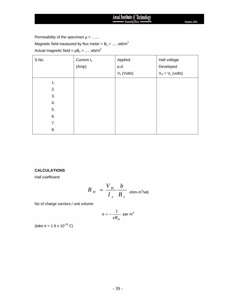
Permeability of the specimen µ = ……

Magnetic field measured by flux meter = Bz = …. wb/m2

Actual magnetic field = µBz = …. wb/m2

S.No. Current Ix(Amp)

Applied

p.d.

Vx (Volts)

Hall voltage

Developed

VH = Vy (volts)

1.

2.

3.

4.

5.

6.

7.

8.

CALCULATIONS

Hall coefficient

zx

HH B

bI

VR = ohm-m3/wb

No of charge carriers / unit volume

HeRn 1

−= per m3

(take e = 1.6 x 10-19 C)

- 39 -

Hall angle φ = dI

VV x

x

H . Radians

Mobility mµ = φ/Bz radians m2/wb

RESULTS From the graph between VH and Ix find hall coefficient, which corresponds to the slope of the straight line and given by

(A) Half coefficient RH = …….. ohm …. M3/weber

(B) No. of charge carriers/m3 = ….

(C) Hall angle = …. Radians

(D) Mobility mµ = ….. radians m2/wb Precautions.

I. Since hall voltaGE developed is very small, so it should be measured very carefully and the millivoltmeter used should be quite sensitive.

2. In finding RH from relation RH =

zx

H

Bb

IV .

The variations of VH w.r.t. Ix should be preferred over variation of VH w.r.t. Bz as it is difficult to measure Bz very accurately.

3. Find the resistance of the specimen for various values of magnetic fields using the relation R = Vx/Ix as the resistance of the specimen changes with the variation of applied magnetic field due to the variation of mobility of the charge carriers.

- 40 -

SPACE USED FOR STUDENTS WORK AREA

- 41 -

REST OF THE EXPERIMENTS ARE IN PART-II

- 42 -

EXPERIMENT 7 AIM : To find the co-efficient of thermal conductivity of a bad conductor by Lee’s method.

APPARATUS USED : Lee’s disc apparatus, two 1/10°C thermometers, circular disc of the specimen of a bad conductor, (ebonite or card board), a stop watch, a screw gauge, vernier calipers etc.

THEORY : On passing steam through the cylindrical vessel a steady state is reached soon. In this condition the rate at which heat is conducted across the specimen disc is equal to the rate at which heat is emitted through the exposed surface of the lower disc. If K is the co-efficient of thermal conductivity of the material of bad conductor, d its thickness and r its radius; θ1 and θ2 the constant readings of the thermometers T1 and T2 in the steady state, then rate at which heat is conducted across the disc of the material

( )d

rKQ 212 θ−θπ

=

If M is the mass of the metal disc, s the specific heat of its material, then rate of cooling at θ2 is equal to

dtdθ

= Ms

dtdθ

is the rate of fall of temperature at θWhere 2

( )dtdMs

drK θ

=θ−θπ 212

( ) dtd

rMsdK θ

θ−θπ=

212 Or

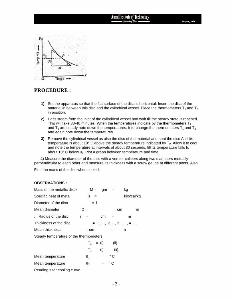
The rate of cooling is found by heating the metal disc to a temperature about 10° C above the steady temperature θ2, it is then allowed to cool and tempetarure is noted after every 30 seconds till the temperature falls to about 10° C below θ2. A graph is then plotted between the temperature and time. A tangent is drawn at a point P corresponding to θ2. The slope of the tangent gives the

value of dtdθ

corresponding to temperature θ2.

- 1 -

PROCEDURE :

1) Set the apparatus so that the flat surface of the disc is horizontal. Insert the disc of the material in between this disc and the cylindrical vessel. Place the thermometers T1 and T2 in position.

2) Pass steam from the inlet of the cylindrical vessel and wait till the steady state is reached. This will take 30-40 minutes. When the temperatures indicate by the thermometers T1 and T2 are steady note down the temperatures. Interchange the thermometers T1 and T2 and again note down the temperatures.

3) Remove the cylindrical vessel as also the disc of the material and heat the disc A till its temperature is about 10° C above the steady temperature indicated by T2. Allow it to cool and note the temperature at intervals of about 30 seconds, till its temperature falls to about 10° C below θ2. Plot a graph between temperature and time.

4) Measure the diameter of the disc with a vernier calipers along two diameters mutually perpendicular to each other and measure its thickness with a screw gauge at different ponts. Also

Find the mass of the disc when cooled.

OBSERVATIONS :

Mass of the metallic disck M = gm = kg

Specific heat of metal s = kilo/cal/kg

Diameter of the disc = 1. .

Mean diameter D = cm = m

∴ Radius of the disc r = cm = m

Thickiness of the disc = 1…., 2…., 3……, 4…..

Mean thickness = cm = m

Steady temperature of the thermometers

T1 = (i) (ii)

T2 = (i) (ii)

Mean temperature θ = ° C 1

= ° C Mean temperature θ2

Reading s for cooling curve.

- 2 -

No. of obs.

1 2 3 4 5 6 7 8 9

Time in seconds

30 60 90 120 150 180 210 …. ….

Temp. of disc

dtdθ

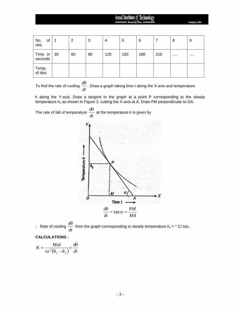
To find the rate of cooling . Draw a graph taking time t along the X-axis and temperature

θ along the Y-axis. Draw a tangent to the graph at a point P corresponding to the steady temperature θ2 as shown in Figure 2. cutting the X-axis at A. Draw PM perpendicular to OA.

dtdθ

The rate of fall of temperature at the temperature θ is given by

MAPM

dtd

=α=θ tan

dtdθ

from the graph corresponding to steady temperature θ∴ Rate of cooling 2 = ° C/ sec.

CALCULATIONS :

( ) dtd

rMsdK θ

×θ−θπ

=21

2

- 3 -

PRECAUTIONS :

Thickness d of the disc of the material should be measured at a number of places on its surface.

1.

The diameter of the disc should be equal to that of the cylindrical vessel and the metallic disc and should be measured in two perpendicular directions.

2.

The thermometers should be placed close to the face of the disc of the specimen. 3.

There should be a good thermal contact between the disc of material and the lower surface of the cylindrical surface and the upper surface of the circular metallic disc. If necessary glycerine may be applied between the surfaces.

4.

The steady state temperatures should be recorded only when the readings of T5. 1 and T2 remain constant after an interval of about five minutres.

- 4 -

SPACE FOR STUDENTS WORK AREA

- 5 -

EXPERIMENT 8

AIM : To determine the capacitance of a capacitor by discharging it through voltmeter.

APPARATUS USED : A capacitor of large capacitance more than 64 µF, a high resistance volt m (sensitivity more than 1000 ohm per volt) and range 300 volt, two tap keys, D.C. regulated power supply capable of giving more than 250 volt and a stop-watch.

PROCEDURE :

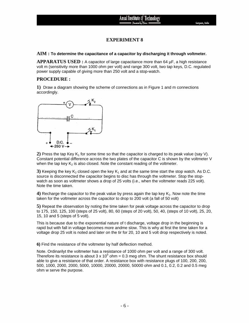
1) Draw a diagram showing the scheme of connections as in Figure 1 and m connections accordingly.

2) Press the tap Key K1 for some time so that the capacitor is charged to its peak value (say V). Constant potential difference across the two plates of the capacitor C is shown by the voltmeter V when the tap key K2 is also closed. Note the constant reading of the voltmeter.

3) Keeping the key K2 closed open the key K1 and at the same time start the stop watch. As D.C. source is disconnected the capacitor begins to disc has through the voltmeter. Stop the stop-watch as soon as voltmeter shows a drop of 25 volts (i.e., when the voltmeter reads 225 volt). Note the time taken.

4) Recharge the capacitor to the peak value by press again the tap key K1. Now note the time taken for the voltmeter across the capacitor to drop to 200 volt (a fall of 50 volt)

5) Repeat the observation by noting the time taken for peak voltage across the capacitor to drop to 175, 150, 125, 100 (steps of 25 volt), 80, 60 (steps of 20 volt), 50, 40, (steps of 10 volt), 25, 20, 15, 10 and 5 (steps of 5 volt).

This is because due to the exponential nature of t discharge, voltage drop in the beginning is rapid but with fall in voltage becomes more andme slow. This is why at first the time taken for a voltage drop 25 volt is noted and later on the tir for 20, 10 and 5 volt drop respectively is noted.

6) Find the resistance of the voltmeter by half deflection method.

Note. Ordinarilyt the voltmeter has a resistance of 1000 ohm per volt and a range of 300 volt. Therefore its resistance is about 3 x 105 ohm = 0.3 meg ohm. The shunt resistance box should able to give a resistance of that order. A resistance box with resistance plugs of 100, 200, 200, 500, 1000, 2000, 2000, 5000, 10000, 20000, 20000, 50000 ohm and 0.1, 0.2, 0.2 and 0.5 meg ohm w serve the purpose.

- 6 -

OBSERVATIONS : Sl.No. Voltage V Loge V Time t Sl.No. Voltage

V Loge V Time t

250

….

….

125

100

….

60

50

…

30

25

…

…

5

Reading of voltmeter Sl.No. Shunt resist. Resistance of

voltmeter Without shunt With shunt

Mean resistance of the voltmeter R = ohm

7) (i) Draw a graph between voltage across the capacitor (V) and time (t), (ii) Also draw a graph between (log V) and time t. e

- 7 -

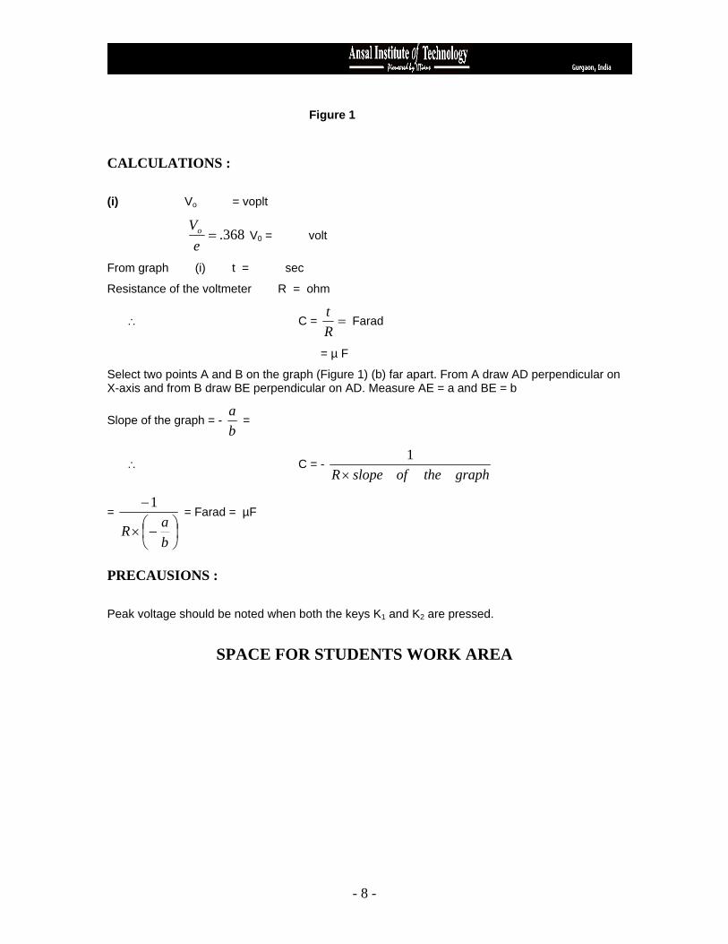
Figure 1 CALCULATIONS : (i) V = voplt o

368.=e

Vo V0 = volt

From graph (i) t = sec

Resistance of the voltmeter R = ohm

∴ C = =Rt

Farad

= µ F

Select two points A and B on the graph (Figure 1) (b) far apart. From A draw AD perpendicular on X-axis and from B draw BE perpendicular on AD. Measure AE = a and BE = b

ba

= Slope of the graph = -

graphtheofslopeR×1

∴ C = -

⎟⎠⎞

⎜⎝⎛−×

−

baR

1 = Farad = µF =

PRECAUSIONS : Peak voltage should be noted when both the keys K1 and K2 are pressed.

SPACE FOR STUDENTS WORK AREA

- 8 -

EXPERIMENT 9

AIM : Find the internal resistance of leclanche cell using a potentiometer.

Apparatus: A potentiometer, a battery, leclanche cell, two one way keys, a sensitive galvanometer, rheostat, two resistance boxes, jockey, an ammeter, a voltmeter, connection wires, sand paper etc.

Theory. Let the p.d. across the terminals of the cell when no current is drawn from it be E and the p.d. when it sends a current to the resistance S be V, then we have

Internal resistance of the cell

SV

VEr ×−

=

- 9 -

The values of E and V are determined l in terms of the length of the potentiometer wire,

Let l1 is the length of the wire to the point where a balance point is got in an open circuit, then

2.. lIV ρ=

SV

VEr ×−

= We have the relation

Sl

llr ×

−=

2

21

Knowing l1, l2 and S the internal resistance of the cell can be found. Procedure Draw diagram showing the scheme of connection Figure (1) and make the connections accordingly. Take out 5000 R from resistance box R.

Figure (1)

2. To test the connections. Introduce the plug in the key K1 and keep K2 open. Press the jockey at the zero end and note the direction of deflection.

Now put the jockey at the other end, if the direction of deflection opposition to that in the first case, the connections are correct. If the direction of deflection is the same, then increase the current in the main circuit till the deflection in the second case is reversed.

3(a) Move the jockey along the wire to find a point where the galvanometer gives zero. Insert the 5000 ohms plug and find the null point accurately as at X. Note that length l1 of the wire and the current in the ammeter. Put in the key K2 and take out 1 ohm plug from the resistance box S and make all other plugs tight. Find the balance point again as at Y and note the corresponding length l2. Repeat twice for the same value of the current in the auxiliary circuit and same shunt resistance in a similar manner to avoid any error.

- 10 -

(b) Put the plugs from the keys K1 and K2. Wait for some time, put the plug in the key K1 and find l1 keeping the current same in a similar manner. Put in the plug in the key K2, take out a resistance of 2, 3, 4 ohms and find the length l1 in each case.

4. Take similar reading by varying the current in the main current.

Observations

Position of null point S.No.

Without shunt With shunt

Ammeter reading

(a) (b) Mean l

(a) (b) Mean I1 2

1

2

3

1

2

3

Precautions

1. The e.m.f of the auxillary batter should be constant and always more than the e.m.f of the cell, whose internal resistance is to be found out.

2. The positive pole of the battery and the positive pole of the cell must be connected to the terminal on the zero side of the potentiometer wire.

3. The rheostat should be of a low resistance and the current must be changed to get the nill point at a desired length.

The current should remain constant for each of readings.

4. The current should be passé donly for the duration it is necessary, otherwise the balance point will go vary.

The internal resistance of a Leclanche cell is not constant but increases with the current drawn from the cell. So to get concordant readings the resistance form the resistance box S must be changed by a small amount.

- 11 -

SPACE FOR STUDENTS WORK AREA

- 12 -

EXPERIMENT 10

AIM : To draw the V-I characteristics of a forward and reverse bias junction diode and to draw the load line

APPRATUS USED : A junction diode [BY 127], millimeter (0-500 mA), voltmeter (0 – 3 V), battery, key, rheostat, micro-ammeter (0-100 µA), voltmeter (0-100V), a D.C. power supply c of giving about 100 volt supply.

PROCEDURE (i) Forward bias characteristics.

- 13 -

1. Draw a diagram showing the scheme of a function as in Figure 1 and make connections accordingly.

Figure – 1

2. Adjust the position of the variable contact of the rheostat so that the voltmeter reads zero, increase the voltage in steps of 0.2 volt and note the voltmeter as well as the correspondence millimeter reading for each setting upto the full range of the battery.

Figure – 2

(ii) Reverse bias characteristics. 1. Draw a diagram showing the scheme of connections figure 2 and make connections accordingly. Starting from zero volt first increase the voltage in of one volt and then in steps of 5 volt. Note the corresponding current in micro-ammeter. D graph between voltage and current taking the voltage for forward bias along the +X-axis and ….. along +Y-axis and for reverse bias the voltage along the – X-axis and current along – Y-axis. A …… graph is shown in figure (4)

Observations

Forward bias Reverse bias S.No.

Voltmeter reading Current in mA Voltmeter reading Current in mA

- 14 -

Precautions

1. In a forward bias characteristic the position of the rheostat should be add…. so that the voltmeter reading is zero. The voltage then should be increased in steps of 0.2 voltmeter.

2. In reverse bias characteristics, the voltage should be increased in steps of 1 volt starting from reading int eh beginning and then in steps of 5 volt.

3. … Load line a diode-circuit. Consider the circuit shown in Figure (3) where the diode is based by a source of voltage V. If the source has a negligible (zero) resistance V = V + IRL …… Vo is the voltage drop across the diode, I the cuurent through the circuit and RL the load …. Distance

LD

L RVV

R+

1I = ……………………………………………………………..(i)

.

Figure – (3)

cmxy +=4. This is an equation of the type the equation of a straight line. Hence a graph between ….. along the Y-axis and V taken along the X-axis is a straight line. D

LRVI =If V = 0 the, D

This gives the point A on the I or Y-axis and represents the maximum value of the current called

function current LR

VI =

= V If I = 0 VD

This gives the point B on the V or X-axis and represents the maximum value of VD D corresponding to zero current called the cut off voltage.

The straight line joining AB is called the load-line.

If we draw a forward bias static characteristics of the diode also alongwith the load line, then the intersection of the static characteristics curve with the load-lien gives the operating point or

- 15 -

Quiescent pont Q. The point Q represents the current through the load resistance RL and the corresponding value of V the voltage drop across the diode. D

LRVI =To draw the load line. To find the pint A, short circuit the diode so the and measure the

current. To find the point B measure the voltage across the source in open circuit. Join the point A and B, then AB is the load line.

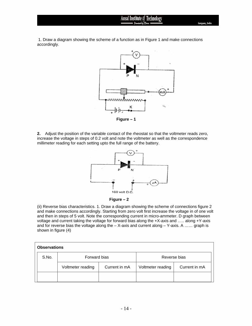
Figure (1) Zener diode. A Zener diode is a silicon crystal diode which conducts in the reverse direction at a certain fixed voltage. It is a highly doped, P-N junction having a high back resistance.

As show in in Figure (4), it is found that when a reverse bias is applied to a crystal diode a very small reverse current (known as leakage current) flows due to high reverse resistance. As the value of the reverse bias is increased, a small current due to minority carriers flows in the circuit. As the reverse bias is increased further, a stage reaches when the applied field is so high that a large number of co-valent bonds are broken with consequent abrupt increase in current. Further, the electrons are also accelerated to high velocities due to the large field and bring about ionization by collision ….. at most of the crystal. The electrons … produced are again

Figure – (4)

Accelerated produce more free electrons due to there ionization (by collision). The process is known as avalanche process and gives rise to a very large currer.. the diode and the junction is said have a breakdown.

The value of reverse voltage which breakdown occurs is called breakdown voltage or Zner voltage.

Due to the large increase in current the back resistance drops to a very low value. After the breakdown has current the voltage across the junction remains constant over a fairly with range.

A Zener diode can be used a Voltage – regulator to provide a constant voltage from a source whose voltage may vary over a sufficient range. The Zener voltage depends upon the semi-conductor material, amount of doping and method of producing the P-N junction. Zener diodes can be obtained with breakdown voltage ranging from 2 volt to several hundred volts by adjusting the concentration of the impurity in the materials producing the P-N junction.

- 16 -

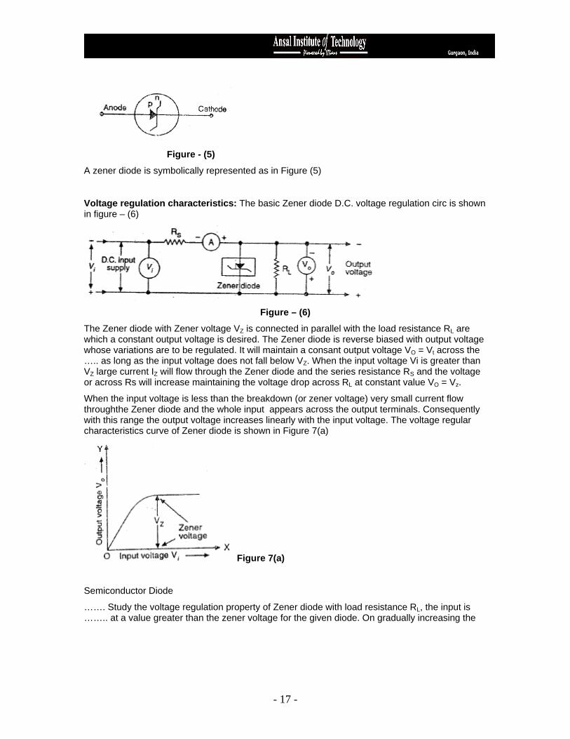
Figure - (5)

A zener diode is symbolically represented as in Figure (5)

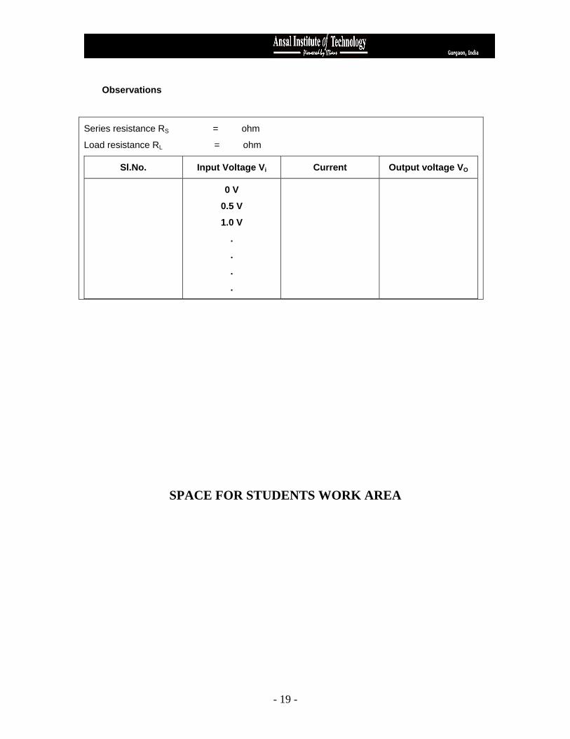
Voltage regulation characteristics: The basic Zener diode D.C. voltage regulation circ is shown in figure – (6)

Figure – (6)

The Zener diode with Zener voltage V is connected in parallel with the load resistance RZ L are which a constant output voltage is desired. The Zener diode is reverse biased with output voltage whose variations are to be regulated. It will maintain a consant output voltage VO = Vt across the ….. as long as the input voltage does not fall below VZ. When the input voltage Vi is greater than V large current I will flow through the Zener diode and the series resistance RZ Z S and the voltage or across Rs will increase maintaining the voltage drop across RL at constant value VO = Vz.

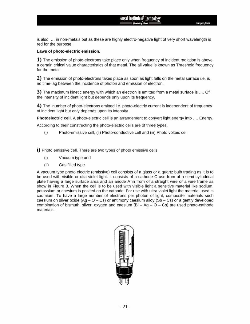
When the input voltage is less than the breakdown (or zener voltage) very small current flow throughthe Zener diode and the whole input appears across the output terminals. Consequently with this range the output voltage increases linearly with the input voltage. The voltage regular characteristics curve of Zener diode is shown in Figure 7(a)

Figure 7(a)

Semiconductor Diode

……. Study the voltage regulation property of Zener diode with load resistance RL, the input is …….. at a value greater than the zener voltage for the given diode. On gradually increasing the

- 17 -

Figure 7(b)

Resistance it is found that for small values of load resistance the output voltage increases linearly …. Load. For large values of load resistance the output voltage remains constant. The variation of voltage with load resistance is shown in Figure 7(b).

To study Zener diode voltage regulating characteristics.

Apparatus. A variable D.C. supply, a Zener diode, voltmeter and an ammeter with ranges coding to zener diode supplied, tow resistance boxes RS and RL, connecting wires etc.

PROCEDURE

1. Draw a diagram showing the scheme of connections as in Figure 6 and make sections accordingly.

Note: The Zener diode must be connected in reverse bias.

2. Introduce a fixed resistance RS (100 to 500Ω) in series with the diode. Keep it constant throughout the experiment. Introduce a load resistance RL of about 1000 ohm.

3. Starting from very low values of input voltage increase it in small steps well above the zener voltage for the given diode. For each observation note the input voltage Vi and corresponding output voltage VO. Also note the current in the input circuit.

4. Plot a graph between input voltage V taken along the X-axis and output voltage Vi O taken along Y-axis. The graph is as shown in figure 7(a).

5. Voltage regulation with load. Keep the input voltage at a value more than the zener voltage. Starting from a small value of about 50 ohm for RL, increase it in steps of 50-100 ohm. Note the distance and the corresponding values of output voltage.

6. Plot a graph between load resistance RL taken along the X-axis and output voltage VO taken …. Y-axis.. The graph is as shown in figure 7(b).

- 18 -

Observations

Series resistance RS = ohm

Load resistance RL = ohm

Sl.No. Input Voltage V Current Output voltage Vi O

0 V

0.5 V

1.0 V

.

.

.

.

SPACE FOR STUDENTS WORK AREA

- 19 -

EXPERIMENT 11

AIM : To find the value of Planck’s constant and photo electric work function of the wcall of the cathode using a photo-electric cell.

APPRATUS USED : A vacuum type photo-cell enclosed in tight box; (R, C, A. 935 or its equivalent), 6 volt apply, a voltmeter (0-3 volt capable of reading up volt), a rheostate, a moving coil reflecting type galvanometer with lamp and scale arrangement, …. Key, a mercury lamp, light filters (red, yellow, green, blue, violet)

THEORY : Photo-electric effect. It is phenomenon of emission of electrons from a metal surface light of suitable wavelength falls on it. The electrons emitted are known as photo electrons. Are metals like sodium, potassium and caesium emit electrons even when visible light falls on whereas zinc, cadmium etc. are sensitive only to ultra – violet light. Light of shorter wavelength are effective in producing photo-electrons than light of longer wave length. The effect

- 20 -

is also … in non-metals but as these are highly electro-negative light of very short wavelength is red for the purpose.

Laws of photo-electric emission.

1) The emission of photo-electrons take place only when frequency of incident radiation is above a certain critical value characteristics of that metal. The all value is known as Threshold frequency for the metal.

2) The emission of photo-electrons takes place as soon as light falls on the metal surface i.e. is no time-lag between the incidence of photon and emission of electron.

3) The maximum kinetic energy with which an electron is emitted from a metal surface is …. Of the intensity of incident light but depends only upon its frequency.

4) The number of photo-electrons emitted i.e. photo-electric current is independent of frequency of incident light but only depends upon its intensity.

Photoelectric cell. A photo-electric cell is an arrangement to convert light energy into …. Energy.

According to their constructing the photo-electric cells are of three types.

(i) Photo-emissive cell, (ii) Photo-conductive cell and (iii) Photo voltaic cell

i) Photo emissive cell. There are two types of photo emissive cells

(i) Vacuum type and

(ii) Gas filled type

A vacuum type photo electric (emissive) cell consists of a glass or a quartz bulb trading as it is to be used with visible or ulta violet light. It consists of a cathode C use from of a semi cylindrical plate having a large surface area and an anode A in from of a straight wire or a wire frame as show in Figure 3. When the cell is to be used with visible light a sensitive material like sodium, potassium or caesium is posited on the cathode. For use with ultra violet light the material used is cadmium. To have a large number of electrons per photon of light, composite materials such caesium on silver oxide (Ag – O – Cs) or antimony caesium alloy (Sb – Cs) or a gently developed combination of bismuth, silver, oxygen and caesium (Bi – Ag – O – Cs) are used photo-cathode materials.

- 21 -

Figure 1

The current in a vacuum type (emissive) cell is small. To increase the current the cell is 1 with an inert gas like neon or argon at a pressure of a few millimeter of mercury. Such a cell is kr as a gas-filled cell.

A simple circuit showing the working of a c showin in figure 1. If a light of suitable wavelength is allowed to fall on the cathode C it gives out electrons. When the anode A is maintained at a photo potential the electrons are attracted towards it …. Conventional current flows in the external circuit shown. If A is maintained at a negative potential electrons are repelled by it and a smaller nu … reaches it. The current, therefore, decreases and certain negative potential no photo electrons real. This potential is called stopping potential or c voltage.

If Vs is the stopping potential, m, e and v mass, charge and maximum velocity of the ejected electrons respectively, then

2

21

ms mveV =

meV

v sm

2= Or

The velocity of ejected electrons increases with increase in frequencies of the incident light, the frequency is below a certain critical value called threshold frequency no electrons are eject. If v0 is the threshold frequency the energy required to eject the electrons just out of the surface given by

= hvω0 0

Where ω is known as photo electric work function. 0

In photo electric effect all or none of the energy of the incident photon is transferred electron in the metal. If, therefore, light of frequency v > v0 falls on the photo – sensitive matel part of the energy of the incident photon is used by the electron to come out of the metal …. (photo-electric work function) and the rest is stored in it as kinetic energy.

02

21

ω+= mmvhv∴

0hveVs + =

- 22 -

0vehv

ehVs −=Or

Thus a graph between stopping potential Vs and frequency of incident light v is a straight. The slope of the straight line

eh

=θtan

θ= taneh Or

vVs

ΛΛ

= e

PROCEDURE :

1) Draw a diagram showing the scheme of connections in figure 1 and connectivity. Arrange the mercury lamp and the photo-cell as shown and set up the lamp and scale measurement of the galvanometer so that the spot of light moves freely on the scale.

Figure - 2

With the box closed (no light falling on the photo-cell) adjust the sliding contact to the extreme point P so that when the key K is introduced the voltmeter reads zero. Adjust the position of the

galvanometer scale so that the spot of light with its central cross-wire is at zero graduation.

- 23 -

Figure 3

Place the violet filter (λ = 4050 A) in front of the photo cell and switch on the mercury vapour lamp. Adjust the distance of the lamp so as to get a reasonable deflection on the galvanometer scale. Note the reading of spot of light on the scale and also that of the voltmeter. 2) Slowly move the sliding contact towards Q (negative end of the battery) so that a negative potential of 0.05 V is applied to the anode A of the photo-electric cell. The deflection will slightly decrease. Note the scale reading and meter reading. Go on increasing the negative potential applied to the anode A in steps of 0.05 volt on noting the voltmeter reading and corresponding scale reading until the spot of light returns to position. Take at least three more readings by further increasing the negative potential in steps 05 volt. 3) Repeat the experiment with blue (λ = 4360 A), green (λ = 5780 A) and red (λ = 6910 A) Filters.

Scale deflection with Sl. No. Voltmeter reading (Negative) Violet filter Blue filter Green filter Yellow

filter Red filter

0 volt

-0.05

-0.10

-0.15

….

…..

- 24 -

5) For each filter draw a graph between voltmeter reading (negative anode voltage) and deflecting in cm. From the graph, find the value of stopping potential V1 for which scale deflection is zero corresponding to each wavelength and record.

Note. Alternatively the value of stopping potential corresponding to each filter may be form directly without plotting the graph. For this purpose the negative potential applied to the anode of photo-cell is increased very slowly so that the deflection on the galvanometer scale just

becomes zero. The corresponding voltmeter reading gives the stopping potential for each filter.

Filter Violet Blue Green Yellow Red

-10 -10Wavelength λ 4050 x 10 m 4360 x 10 m 5460 x 10-10 m 5780x10-10 m 6910 x 10-10 m

Frequency

λc

V =

Stopping pot V

s

6) Plot a graph between stopping potential Vs taken along the Y-axis and corresponding frequency v taken along the X-axis. The graph is a straight line as show in Figure 3. Take two points P1 and P sufficiently apart on the straight line. Find the values of stopping potentials V2 1 and V2 frequencies v1 and v2 corresponding to P1 and P2.

vV

vvVV s

ΔΔ

=−−

12

12Slope of the graph = tan θ = = volt sec

-19 C Now e = 1.59 x 10

∴ Plank’s constant h = e tan θ

vV

vV ss

ΔΔ

××=ΔΔ −191059.1 = e

= Joule sec.

Threshold frequency (corresponding to point A) v0 =

Photo-electric work function w0 = hvo = Joule

Photo-electric work function (corresponding to point B)

= OB electron volt

PRECAUTIONS :

1) While adjusting the galvanometer reading at zero mark and voltmeter reading 0 volt,no light should fall on the photo-cell .

2) The distance between the mercury lamp and the photo-cell should be kept constant during experiment .

- 25 -

SPACE FOR STUDENTS WORK AREA

- 26 -