Embed Size (px)
Citation preview

Computational Optimization and Applications, 33, 7–49, 2006c! 2006 Springer Science + Business Media Inc. Manufactured in The Netherlands.
DOI: 10.1007/s10589-005-5957-4
A Local Relaxation Approach for the Sitingof Electrical SubstationsWALTER MURRAY" [email protected] of Management Science and Engineering, Stanford University, Stanford, CA 94305-4026
UDAY V. SHANBHAG [email protected] of Mechanical and Industrial Engineering, Urbana, IL 61801
Received March 10, 2005; Revised June 27, 2005; Accepted July 6, 2005
Abstract. The siting and sizing of electrical substations on a rectangular electrical grid can be formulatedas an integer programming problem with a quadratic objective and linear constraints. We propose a novelapproach that is based on solving a sequence of local relaxations of the problem for a given number ofsubstations. Two methods are discussed for determining a new location from the solution of the relaxedproblem. Each leads to a sequence of strictly improving feasible integer solutions. The number of substationsis then modified to seek a further reduction in cost. Lower bounds for the solution are also provided by solvinga sequence of mixed-integer linear programs. Results are provided for a variety of uniform and Gaussian loaddistributions as well as some real examples from an electric utility. The results of GAMS/DICOPT, GAMS/SBB,GAMS/BARON and CPLEX applied to these problems are also reported. Our algorithm shows slow growth incomputational effort with the number of integer variables.
1. Introduction
An important planning problem faced by electric utilities concerns where to placenew substations to meet future electrical load. The planning objective is to minimizethe cost of new substations and the electrical losses when operating the system. Theconstraints include Kirchhoff’s law equations, voltage bounds and capacity boundson the current at substation nodes. The electrical load supported by the grid and thelinkage impedance are known. Kirchhoff’s law leads to constraints (called the load-flowequations) that relate the voltages and the currents at the nodes through the admittancematrix. The problem may be formulated as a mixed-integer programming problem with aquadratic objective and linear constraints. By introducing a novel relaxation, we attemptto solve such a problem by solving a sequence of quadratic programs with continuousvariables.
The paper is organized into five sections. Section 2 discusses some of the earlyresearch in this area. Section 3 gives a formulation of the problem, while in Section 4our new algorithm is described. Section 5 describes different relaxations of the originalproblem that provide a means of obtaining an initial feasible solution and deriving lowerbounds on cost. Results of applying our new algorithm on a variety of test and realworld problems are given in section 6. To allow a comparison, Section 6 also givesthe results of applying GAMS/DICOPT, GAMS/SBB and CPLEX to the smaller problems.
"To whom correspondence should be addressed.

8 MURRAY AND SHANBHAG
Figure 1. The substation siting optimization problem: The figure on the left shows the placement ofexisting or fixed substations and new substations. On the right, the load or current distribution on the grid isshown.
The last section lists the contributions and conclusions of this study and proposes somefuture work.
2. Past research
A useful introduction to the problem is provided in Willis et al. [29]. This referencediscusses the problem briefly and focuses on some specific aspects such as feeder layout,cable sizes and load distribution across the feeders and substations (figure 1). A secondpaper by the same authors [30] discusses the the variety of methods that can be used tosolve the problem. For example, transshipment algorithms convert the electrical networkproblem into one for which network flow algorithms can be applied.
2.1. Transshipment methods
One of the earliest references of an optimal planning approach toward the design ofelectrical networks is by Knight [15]. Based on a given set of geographical locations,a minimum cost network design was obtained using a network flow algorithm (Ahujaet al. [3] provide an excellent review of network flow algorithms). The objective functionaccounted for circuit length and apparent power and the constraints included securityand switchgear limitations. Similar approaches are also seen in the following references[6, 8, 13].
In [28], Wall et al. use a transshipment algorithm to determine decisions conditionalon a choice of integer variables. A branch-and-bound algorithm selects the optimalsolution from the candidate solutions generated by the transshipment code. Capitalcosts are included for potential substations. Note that the essential problem formulationfor the transshipment code is similar to that used by Adams and Laughton [2]. The sameauthors present more details on the embedded transshipment algorithm in [27].
Sharif et al. [25] give an algorithm that used both mixed integer linear programming(MIP) and spanning tree methods to estimate future expansion paths for a radial

LOCAL RELAXATION APPROACH 9
distribution network. The general methodology comprises two steps: The first, thegeneration of spanning trees to connect the source to the demand nodes, and second, aMIP approach to ascertaining which spanning tree to use as the optimal solution.
2.2. Non-transshipment algorithms
El-Kady [8] modeled the planning of distribution substations and associated feedersover time. Marshall et al. [17] solved a distribution planning problem by a slight mod-ification in the objective function. The costs in this particular methodology arose fromcabling, switchgear and the incremental costs of building an extra circuit to a loadnode. This ensures that every load point has some security of supply; if one circuitgoes down, another supplies it with power. The cost of losses was not included inthis study. Provisions were made to ensure the security of the network. The solutionmethodology adopted is that of maximizing the Lagrangian dual using the NETOPTprogram.
Yahav and Oron [32] accounted for the nonlinear costs of losses and constructionthrough the solution of a nonlinear program using the off-the-shelf solver GINO (it usesthe generalized reduced gradient solver GRG2 by Lasdon and Waren [19]. New feederroutes and substation locations are the optimal decisions of the mathematical program.Amongst the more restrictive assumptions made are the linear relationship betweenlosses and distance as well as the ignoring of voltage constraints.
2.3. Mixed-integer nonlinear programs
It is shown in Section 3 that the SSO problem may be formulated as the followingmixed-integer quadratic program:
where Q is a positive semidefinite matrix. Part of matrix A problem has network structurein that network is represented by arectangular grid. The MIQP is a special case of amore general class of problems called mixed-integer nonlinear programs or MINLPs.These problems fall under a larger class of hard optimization problems called NP-hardproblems [20]. No convenient optimality conditions exist for such optimization problemsand one has to find an optimal solution and then verify that the solution is indeed optimal.In fact, such verification may require an exponential number of iterations even if onewere to start from a globally optimal solution.
One of the more common approaches to solving such MINLPs is to apply branch-and-bound methods. Such methods solve continuous relaxations of the MINLPs and

10 MURRAY AND SHANBHAG
partition the feasible region to avoid fractional integer solutions. Leyffer’s results [16]conclude that the computation times grow exponentially with the number of integervariables. The GAMS/SBB solver on the GAMS platform represents one implementationof a branch-and-bound method.
This approach contrasts sharply with a method that alternates between solving amixed-integer linear programming problem and a nonlinear programming problem. Themaster problem may be defined by outer-approximation [7] or by using the ideas ofgeneralized Benders decomposition [9]. Either case results in a mixed-integer linearprogram for the master problem. The solution to the master problem provides a newestimate of integer variables y, which are subsequently used in an NLP (nonlinearprogram) subproblem. The solution to the NLP subproblem provides a new estimateof the continuous variables x. The master problem provides a lower bound to theoptimal solution and these bounds are used to test for termination. Leyffer [16] discussesan example that demonstrates that the outer-approximation algorithm may take anexponential number of iterations. Duran and Grossmann [7] forms the basis for theGAMS/DICOPT solver in GAMS.
Leyffer’s thesis provides a useful literature review into alternative approaches tosolving MINLPs, such as the use of linearizations [4], rounding [23], or even exten-sions of sequential quadratic programming (SQP) in the discrete domain [5]. A recentdoctoral thesis by Ng [22] focused on homotopy methods to solve certain classes ofMINLPs.
The GAMS/BARON solver is an efficient method for obtaining global optima of nonlin-ear integer programs. In [26], Tawarmalani and Sahinidis present a detailed developmentof the steps of this method and a commercial implementation is also available [24]. Giventhat the algorithm relies on branch-and-bound technology, one can expect difficultieswhen the problem has a large number of discrete variables. In [21], the authors comparethe performance of over 1000 test problems with sizes as large as a thousand variables.Based on these tests, they find that GAMS/BARON is the most robust with GAMS/OQNLP
close behind. We also report the performance of GAMS/BARON on some at the smallertest problems. The other solvers GAMS/OQNLP [1] and LINGO were not available to usand have not been compared.
Our interest is in large-scale MIQPs; the SSO problem even for the most modestproblems sizes has at least a 100 (10 # 10) integers and may go as high as 10,000(100 # 100) integers. As we show in the sections to follow, the problem has a distinctstructure that forms the basis for our algorithm. We also provide a polynomial boundon the work required for a major iteration of the algorithm. Such a bound is useful forensuring that there is slow growth in computational time with the number of integervariables.
3. Formulation of the problem
The core of the constraint system of the SSO problem is the load-flow system. Whilethis shall be developed in greater detail in Section 5, the admittance matrix and some ofits properties are described next. This leads into a description of some nonlinear integerprogramming formulations of the problem.

LOCAL RELAXATION APPROACH 11
3.1. Variables and parameters
m # n Dimension of rectangular electrical grid
I , V, ! Vector of nodal currents, voltages and loads1
Y, ly Admittance matrix and linkage admittance (same for all linkages)
Ccap, Closs Cost of a new substation and network losses
Scap Capacity of a new substation
Nss, NL Set of nodes occupied (not occupied) by substations
Vl Lower bound on voltage
nload Number of load-bearing nodes on electrical grid
minss, maxss Minimum and maxmimum number of substations
n"ss Optimal number of substations
loadS Total load borne by the electrical grid
" Threshold parameter in CG (center of gravity) method
xcg, ycg x and y coordinates of the center of gravity in the CG method
N(i) Set of nodes neighboring node i. For instance in a 4 # 4 grid, the neighbors of node 1 arenodes 2 and 5 viz. N(1) = {2, 5}.
e, ek Column of ones and kth unit vector
Zss The “null space” matrix associated with the positions of substations, both new and old. Thematrix comprises rows of the identity matrix corresponding to the nodes at which nosubstations are located. The numbering is done row-wise. For example, if there were onesubstation in the center of a 3 # 3 grid, then Zss would be the identity matrix I9 $ %9#9
with row 5 missing
Yss The “range space” matrix associated with the positions of substations, both new and old. Thematrix comprises rows of the identity matrix corresponding to the nodes at whichsubstations are located. For the 3 # 3 grid with one substation in the center, Yss = eT
5
3.2. The admittance matrix
Assuming a DC load-flow model, the current vector I is linked to the voltage vector Vthrough the linear equation
I = Y V, (3.1)
where Y is the admittance matrix. Each node interior to the grid has linkages with nodeson four sides while nodes on the boundaries have correspondingly fewer connections.The admittance matrix captures the relationship of a node with its neighbors. Therefore,each row of (3.1) can be thought of as a current-balance relationship in which the currentat a particular node is equal to the sum of the current flows along the links connectedto it. It follows that the admittance matrix Y can be represented as a symmetric blocktridiagonal matrix
Y =
!
"""""#
A1 B1
B1 A2 B2. . .
. . .. . .
Bn&2 An&1 Bn&1
Bn&1 An
$
%%%%%&,

12 MURRAY AND SHANBHAG
Figure 2. Constructing the admittance matrix Y. The captions show how the diagonal elements of the Ymatrix are dependent on the number of linkages to the corresponding nodes.
where the blocks A j , j = 1, . . . , n and B j , j = 1, . . . , n & 1 are tridiagonal anddiagonal in structure, respectively. The diagonal element Yii of any row is equal to thenegative sum of the off-diagonal elements. In particular
Yii = &'
j$N (i)
Yi j ,
where N(i) represents the coordinates of the neighbors of i. Therefore, the row elementsof the admittance matrix sum up to 0. If ly represents the admittance of any link of aregular electrical grid, the admittance matrix blocks are defined as follows:
A1 and An = ly
!
"""""#
2 &1&1 3 &1
. . .. . .
. . .&1 3 &1
& 2
$
%%%%%&,
A2, . . . , An&1 = ly
!
"""""#
3 &1&1 4 &1
. . .. . .
. . .&1 4 &1
&1 3
$
%%%%%&
and B1, . . . , Bn&1 = ly
!
"""""#
&1&1
. . .&1
&1
$
%%%%%&.

LOCAL RELAXATION APPROACH 13
Lemma 3.1. The admittance matrix Y associated with an m # n electrical grid issymmetric and positive semidefinite.
Proof: By Gershgorin’s theorem, #(Y) lie in at least one of the discs with centersYii and radii
(j '=i |Yi j |. Since Yii =
(j '=i |Yi j |,(i , none of the discs extend into the
negative real axis which implies that the eigenvalues are nonnegative. Thus Y is positivesemidefinite. Symmetry of Y follows trivially from its definition. !
One of the important properties of the Y matrix is its rank deficiency as the followinglemma shows.
Lemma 3.2. The column vector of ones is an eigenvector associated with the zeroeigenvalue. In other words, we have Ye = 0.
Proof: This follows directly from the construction of the Y matrix. !
The existence of a zero eigenvalue allows one the voltages to be modified by multiplesof e without impacting the load-flow solution. This can be mathematically stated as
I = Y V = Y (V + ke) = Y V ,
where k is some scalar.We are now ready to prove the main result that the admittance matrix of an m # n
grid, Ym#n, has a rank deficiency of 1 and shall use a constructive argument to do so.We first prove that Y1#n has a rank deficiency of 1. We then show that an augmentationof the grid with nodes and linkages does have not alter the number of zero eigenvalues.
Lemma 3.3. The admittance matrix of a grid of dimension 1 # n has a rank deficiencyof 1.
Proof: The admittance matrix of a 1 # n grid is a n # n matrix given by:
!
"""""""#
1 &1
&1 2 &1. . .
. . .. . .
&1 2 &1
&1 1
$
%%%%%%%&
.
The LDLT factorization of this matrix is given by:
!
"""""""#
1
&1 1. . .
. . .
&1 1
&1 1
$
%%%%%%%&
!
"""""""#
1
1. . .
1
0
$
%%%%%%%&
!
"""""""#
1 &1
1 &1. . .
. . .
1 &1
1
$
%%%%%%%&
.

14 MURRAY AND SHANBHAG
Figure 3. This figure shows the addition of 3 linkages and 2 nodes to the 1 # n grid. The addition occurs inthree steps with the corresponding admittance matrices being called Y1#n, Y2, Y3 and Y4. We prove that eachstep maintains the rank deficiency as 1.
Therefore, the admittance matrix has exactly one zero eigenvalue. !
Lemma 3.4. Let Y1#n represent the admittance matrix associated with a grid ofdimension 1 # n. This grid may be modified as shown in figure 3. Based on figure 3, thecorresponding admittance matrices Y1#n, Y2, Y3 and Y4 have one zero eigenvalue.
Proof:
1. Y1#n ) Y2: The addition of a linkage and a node to the 1 # n grid results in a changein the admittance matrix. The new admittance matrix may be written as
Y2 = Y1#n + D,
where
Y1#n =)
Y1#n 0n,1
01,n 0
*
and D =)
e1eT1 &e1
&eT1 1
*
.
Define
Ln *)
In
eT1 1
*
LOCAL RELAXATION APPROACH 15
We have
LTn Y2 Ln =
+In e1
1
, +Y1#n + e1eT
1 &e1
&eT1 1
,+IneT
1 1
,
=+
Y1#n + e1eT1 & e1eT
11
,
=+
Y1#n1
,.
The nonsingularity of Ln implies that Y2 has one zero eigenvalue.2. Y2 ) Y3: The admittance matrix Y3 may be written as
Y3 = Y2 + D,
where
Y2 =+
Y2
0
,and D =
+en+1eT
n+1 &en+1
&eTn+1 1
,.
Define
Ln+1 *+
In+1
eTn+1 1
,.
We have
LTn+1Y3Ln+1 =
+In+1 en+1
1
, +Y2 + en+1eT
n+1 &en+1
&eTn+1 1
, +In+1
eTn+1 1
,
=+
Y2 + en+1eTn+1 & en+1eT
n+11
,
=+
Y2
1
,,
which implies that Y3 has one zero eigenvalue.3. Y3 ) Y4: Unlike the previous two steps, the grid merely requires an addition of a
linkage without adding any further nodes. The admittance matrix Y4 is then given by
Y4 = Y3 + D,
where
D =+
e2eT2 &e2
&eT2 1
,=
+e2
&1
,+e2
&1
,T
= wwT .

16 MURRAY AND SHANBHAG
The eigenvalues of
#i (Y4) $ [#i (Y3), #i+1(Y3)], i = 1, · · · , n + 1,
where the eigenvalues of Y3 are ordered such that
0 = #1(Y3) < #2(Y3) + · · · + #n+2(Y3).
This follows from Theorem 8.1.8 in [12]. But, we know that Y4 has at least one zeroeigenvalue from Lemma 3.2. It follows that Y4 has exactly one zero eigenvalue.
!
We now state the main result of this section:
Theorem 3.1. The admittance matrix Y of an m # n grid has exactly one zero eigen-value, with corresponding eigenvector e.
Proof: The admittance matrix associated with the 1 # n grid is shown to have exactlyone zero eigenvalue (Lemma 3.3). By using Lemma 3.4 repeatedly, we may constructan admittance matrix associated with an m # n grid. The number of zero eigenvalues ismaintained through these transitions giving us the required result. !
A consequence of this theorem is that we can replace the system
I & Y V = 0
by one in which the last row is omitted. The resulting specification of the load-flowsystem ignores the current in the mnth node. This is specified by the conservationconstraint proved in Lemma 3.5:
mn'
i=1
I i = 0.
For purposes of clarity, our formulation shall maintain the form of the load-flow systemas I = Y V .
Lemma 3.5. The sum of nodal currents(mn
i=1 I i = 0.
Proof: Consider the load-flow system:
( I &Y )+
IV
,= 0.

LOCAL RELAXATION APPROACH 17
Multiplying both sides by eT and using the results from the previous two lemma, weobtain the result as follows:
eT ( I &Y )+
IV
,= 0
( eT &eT Y )+
IV
,= 0
( eT &eT Y T )+
IV
,= 0
( eT 0 )+
IV
,= 0
eT I = 0. !
3.3. Nonlinear integer programming formulation
This section shall formulate the nonlinear integer program of interest. The objectivefunction is the sum of the capital costs of new substations and the cost of electricallosses. The latter is given by ClossV T Y V , where V T Y V represents the electrical lossesin the system and Closs represents the cost per unit of losses. The constraints on voltageand current at a particular node are contingent on whether the node has a substationplaced on it or not.
We define two sets of nodes: Nss is the set of nodes housing new and old substationswhile NL contains all other nodes. These sets are modified through the algorithm.Moreover, the dependency of the constraints on whether i $ Nss or not can be stated interms of binary decision variables. Let yi be such that if i $ Nss then yi = 1, otherwiseyi = 0. Clearly the dimension of y is equal to the number of nodes. Such a specificationallows us to specify the cost of new substations as CcapeT y where Ccap and eT y representthe unit cost of a new substation and the number of new substations, respectively. Theconstraint system comprises the following:
1. The load-flow system I = Y V .
2. The bounds on nodal voltages.3. The specification that a nodal current may be either a variable or a fixed quantity
based on whether the node houses a substation or not.
It follows that the problem may be stated as
18 MURRAY AND SHANBHAG
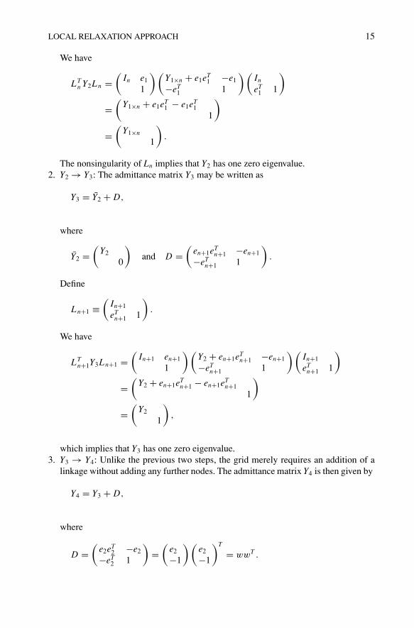
where Scap is the capacity of a new substation. The bounds on V and I can be stated interms of the substation installation decisions y. Such a formulation may be rewritten asfollows:
(SSO) is a mixed-integer programming problem with a quadratic objective. Nonlin-ear integer programming solvers such as GAMS/SBB, GAMS/DICOPT, GAMS/BARON andCPLEX/MIQP may be used to solve (SSO). However, these solvers slow down significantlywhen the number of binary variables exceeds 100 (10 # 10) as we shall describe insection 6.
Our new algorithm can solve problems of the order of (50 # 50) resulting in 2500binary variables with a MATLAB implementation.
4. The substation siting optimization algorithm
The approach adopted in our new method is to mimic linesearch and trust-region methodsfor solving smooth problems in continuous variables. Such algorithms use a localapproximation to the problem to determine an improved estimate of the solution. Inthe case of the substation location problem, the search direction or step translates intoa move to a neighboring node (or possibly remaining at the current node) for all thesubstations.
Although this is a reduced task from that of considering all possible moves, thereare still 9K possible moves, given K new substations, where K is typically 50–150.Limiting the number of substations that can move is clearly suboptimal since theirrelative positions are important and may need to be maintained. For the possible numberof choices to be tractable, the limit on the number of substations allowed to move wouldneed to be very small. In some discrete problems, once the discrete variables have beenspecified, the evaluation of the objective is trivial. Here, it is necessary to solve a largescale quadratic program (QP) to evaluate a trial placement. This clearly limits the numberof trial moves. Simply moving one or a small number of substations is also unlikely tosucceed.
In our new algorithm, we describe how a simultaneous move for all substations isobtained from a local relaxation of the problem. The following is a brief summary ofthe steps given together with their correspondence to the steps of nonlinear programsfor continuous variables.
• Determining an initial feasible solution. Optimization algorithms for continuous vari-ables with linear constraints typically start from an initial feasible point and maintainfeasibility in all iterates. An advantage of such an approach is that the objective is

LOCAL RELAXATION APPROACH 19
then a measure of merit and the iterates provide a strictly monotonically improvingsequence of iterates. In general, determining an initial feasible point to a discreteproblem is hard. However, we provide a method to find such a solution for thisproblem.
• Determining a descent step. For general nonlinear programs, the direction of descentis obtained by solving a system of equations or a quadratic program (QP). Ouralgorithm requires the solution of a local relaxation of the problem that results ina QP.
• Determining the step length. The linesearch algorithm is replaced by one of twopossible methods. Each method uses the information from the local relaxation todetermine a new set of locations with lower objective.
• Termination criteria. While the optimality conditions could be one test of terminationfor a nonlinear program, no such conditions exist for a nonlinear program with integervariables. Thus the termination is based not on having reached an “optimum” but onnot being able to find a better position.
4.1. An initial feasible solution
Determining an initial feasible solution is not difficult since we could saturate the gridwith substations. However, since the number of nodes is substantially larger than theoptimal number of substations, such an approach would result in a very poor initialpoint.
An initial feasible solution is obtained by first solving a global relaxation of theinteger variables in the problem, coupled with a modified objective. The relaxed discretevariables are then rounded up to give an integer solution. Note that by rounding up, weare increasing the resources and hence will not violate constraints on voltage or capacity.The nonzero components of y specify where to place new substations while the numberof nonzero components specifies the number of new substations. Unless steps are takento prevent it, there is a danger in this approach that the number of substations in theinitial feasible solution may be very large.
The modified objective function replaces the capital cost by a smooth function C(y;µ) which is defined as follows
C(y; µ) ='
i
f (yi , µ) ='
i
Ccap(1 & e&µyi )
The variation of f with yi is shown in figure 4. It can be seen that if the capital costassociated with a new substation forms a step function, the function f is a lower boundto this step function. In fact, as
as µ ) ,, f (yi , µ) )-
Ccap, yi > 00, yi = 0 .
It may be noted that such a formulation also admits the convex relaxation in whichf (yi ) = Ccap yi , yi $ [0, 1]. This may be achieved by allowing µ to be a function of yi

20 MURRAY AND SHANBHAG
Figure 4. This figure shows how f(yi, µ) tends to a step function as µ increases. We have shown µ goingfrom 1 to 20. Also shown is the 45 degree line represented by the convex relaxation fC(yi).
and representing the function f as:
f (yi , µ(yi )) = Ccap(1 & e&µ(yi )yi )) = Ccap(1 & e1yi
(loge(1&yi ))yi = Ccap yi .
This function is denoted by fc(yi) and is shown as the diagonal line in figure 4. Thenew formulation of the problem can then be stated as:
where Cmult = Ccap
Closs. Since Ccap and Closs are given, Cmult is fixed. However, for the
feasibility phase it is often beneficial to deviate from the prescribed value. Note that fora small enough Cmult, a substation would be placed at every load node. This would berepresented by the specification: yi = 1,(i $ { j : ! j < 0}.
For large enough values of Cmult, the choice of a single nonzero valued component ofy would be preferred to two or more nonzero components of y, provided both choicesare feasible. Consequently, large values of Cmult force variables onto their lower orupper bounds and no rounding is needed for such variables. Moreover, it reduces thenumber of nonzero elements and hence the number of substations in the initial feasiblesolution.
The resulting solution need not have all yi $ {0,1}. However, any nonzero yi < 1 isrounded to 1. We shall illustrate the impact of changing Cmult on the solution by thefollowing example.

LOCAL RELAXATION APPROACH 21
Example 4.1. Consider an electrical grid of dimension 6 # 6 with a non-uniform loaddistribution (this is described further in Section 6.1). We set µ = 10 and consider threelevels of capital cost: Ccap = 0.001, 0.0005 and 0.0003. The cost of losses is set at unity.The supply of power for case 1 is as follows:
Supply: Case 1
0 0 0 0 0 0
0 0 0 0 0 0
0 0 0 0 0 0
0 0 0.9353 0 0 0
0 0 0 0 0 0
0 0 0 0 0 0
implying that a substation will be placed at position (4, 3).
Case 2. on the other hand has a capacity cost of 0.0005. The power supply distributionis
Supply: Case 2
0 0 0 0 0 0
0 0 0 0 0 0
0 0 0.3991 0 0 0
0 0 1.0000 0 0 0
0 0 0 0 0 0
0 0 0 0 0 0
Case 3. specifies a capital cost of 0.00025 resulting in the following distribution ofsupply:
Supply: Case 3
0 0 0 0 0 0
0 0 0 0 0 0
0 0 0.4347 0 0 0
0 0 0.3528 0 0 0
0 0 0 0 0.0555 0
0 0 0 0 0 0

22 MURRAY AND SHANBHAG
Table 1. Comparison of cost and losses.
Case 1 Case 2 Case 3
Number of substations 1 2 3
Cmult 0.00100 0.00050 0.00025
Cost of losses 0.00170 0.00096 0.00080
Cost of capital 0.00100 0.00100 0.00075
Total cost 0.00270 0.00196 0.00155
and requires the installation of 3 substations with positions (3, 3), (4, 3) and (5, 5). Thecost statistics are provided in Table 1. Note that despite the capital cost falling by nearlya factor of 2 across each case, the number of substations only doubled from case 1 to 2.This corresponds well with the drop in losses. For instance, the losses nearly get halvedfrom case 1 to 2 but do not drop as significantly when another substation is added. Thisis because the third substation has an outflow of only 0.0055 as opposed to 0.4347 and0.3598 from the first two substations.
In practice, this method of obtaining an initial feasible solution has been highlyeffective. Typically, the number of substations in the solution is smaller than the op-timal number, which is beneficial to our search procedure (for the optimal number ofsubstations).
4.2. A local relaxation: “Relax” phase
Given an initial feasible point, we keep the number of substations fixed and attemptto determine their optimal location. As we shall discuss in Section 4.4, the number ofsubstations is adjusted in a second phase. The basic idea is that we wish to determine anew assignment with a lower cost from all possible neighbors of the current assignment.Since each node has eight neighbors, this implies that for k substations, there are (9k&1)possible new assignments. In general, for even small values of k (say 5), this representsa large amount of work in terms of solving the resulting load-flow equations.
To get some guidance on which neighbors are attractive, we introduce new substationsat all neighboring locations. We call this a 9-point stencil (see figure 5). Each stencilcan, at most, bear a load equal to that of the capacity of a single substation. We assumethat the current locations of the substations are sufficiently separated so that the stencilsdo not overlap. It remains to be determined as to what each substation node of the9-point stencil contributes in terms of power. If the outcome is that one substation bearsthe whole load (unlikely), then this is clearly an improvement since it is the solutionof a relaxed problem. However, in the more likely outcome that each substation in the9-point stencil bears some load, we deduce an attractive location of the substation basedon the distribution of the supply across a stencil. We can determine this distribution ofcapacity by solving a QP in continuous variables. Given a placement of new substationson the electrical grid, this implies that we can construct a “null space” matrix Zss anda “range space” matrix Yss, associated with the current set of substation positions (seeSection 3.1). The subproblem to be solved can be stated as

LOCAL RELAXATION APPROACH 23
The objective function represents the total losses across the network. The first twoconstraints represent the load-flow equations. The third constraint specifies that the sumof the currents from the 9 points of a stencil cannot exceed the prescribed substationcurrent capacity plus the total load over the stencil (note that load by convention isassumed to be negative). The last constraint shows the bounds on nodal voltages. Figure5 shows three grids that explain the aforementioned relaxation procedure.
4.2.1. The integer subproblem. The integer subproblem is the solution of the originalproblem with the integer variables fixed at some pre-specified levels. This immediatelyconverts the original mixed-integer QP into a QP in continuous variables. The solutionto this subproblem, along with the current values of the integer variables, represent afeasible solution to the original MIQP. In fact, the cost of the original MIQP is the costof the integer subproblem plus the installed cost of new substations. The solution of theproblem (SSOsubint) gives the voltages at non-substation nodes and the current flows atall substation nodes . The only difference between (SSOsub) and (SSOsubint) is that thelatter problem has a neighborhood defined by N1 or a 1-point stencil instead of a 9-pointstencil, implying no relaxation of substation capacity.
The solution of the local relaxed problem is used to infer a good choice of node to whichto move a specific substation. One possibility is to choose the node that is the mostimportant (has the largest current outflow). In Section 4.3 we describe two alternativestrategies. In both cases, either no move is made or a better feasible solution is found. Weconclude this discussion by noting that solvability of SSOsub and SSOsubint is guaranteedfrom the continuity of their objectives and the compactness of their feasible regions.
Result 4.1. There exists an optimal solution to the subproblems SSOsubint and SSOsub.
Proof: By virtue of the compactness of the feasible regions of SSOsubint and SSOsub
and the continuity of their objectives, an optimal solution to both problems exists basedon Weierstrass’s theorem. !

24 MURRAY AND SHANBHAG
Figure 5. Figure (a) shows a feasible integer solution. The next step demonstrates how the relaxation places“substations” around the current positions. The variables are then given by the flows emerging from these9-point stencils. Figure (c) shows the solution in which the circle size represents the importance of the node.
Figure 6. The CG method: Figure (a) shows the subproblem solution. (b) shows the orthants associatedwith each stencil and the small darkened circles outside the inner stencils represent the centers-of-gravity ofthe stencil. The placement of the darkened circle in the larger circles represents a candidate position of thesubstations. Finally (c) shows the new positions of the substations.
4.3. Finding an improved set of locations: “Shift” phase
The "relax" phase replaces each substation by a 9-point stencil and solves the resultingcontinuous quadratic program. The “shift” phase determines a new set of substationpositions with lower system cost. If such a set cannot be found by the method, thealgorithm terminates with the current integer solution. Two methods shall be presentedfor this purpose:
1. The Center-of-Gravity or the CG method.2. The Assignment method.
4.3.1. The CG method. The coordinates, say xcg and ycg , of the center of gravityassociated with a stencil placed at (i, j) are defined by:
xcg :=( j+1
k= j&1( I(i+1)k & I(i&1)k)(i+1
p=i&1
( j+1k= j&1 I pk
, (4.1)

LOCAL RELAXATION APPROACH 25
ycg :=(i+1
k=i&1( Ik( j+1) & Ik( j&1))(i+1
p=i&1
( j+1k= j&1 I pk
. (4.2)
If (xcg, ycg) is “close” to (i, j) the substation is not moved from (i, j). There are a numberof measures to define “close”. We use a square of size " (where " $ [0, 1]) centered at (i,j). When " = 1, the square is the size of the stencil. For the results reported here, an initialvalue of " = 0.1 was used. This is somewhat conservative since one might expect that" = 0.5 represents the threshold of when it is worthwhile to move a substation. However,the efficiency of the algorithm is such that we can afford to be conservative.
If the center of gravity is outside the square, we identify an orthant in which it lies.The stencil is divided into eight orthants, which are specified as follows. Suppose theline joining the center-of-gravity to the center of stencil k makes an angle $k with thepositive x&axis, where
$k = tan&1+
xk
yk
,.
The angle associated with this CG is given by:
$k =
.//////////0
//////////1
tan&1
+ |xk ||yk |
,, xk, yk > 0,
tan&1
+ |xk ||yk |
,+ %
2, xk > 0 > yk,
tan&1
+ |xk ||yk |
,+ %, 0 > xk, yk,
tan&1
+ |xk ||yk |
,+ 3%
2, yk > 0 > xk .
(4.3)
The candidate substation nodes are defined by:
cand-node =2
0 dk < ",3%16 +$k
%8
4dk - ",
(4.4)
where the central node is numbered as 0 and the bordering nodes are numbered clock-wise, from 1 to 8, starting from the one immediately above the central node. The orthantin which the center of gravity lies identifies a unique node. We restrict our interest to thisnode. In so doing, we have reduced our combinatorial problem from (9k&1) to (2k&1).While the latter is substantially smaller than the former, it will for most cases still betoo large to carry out an exhaustive search.
Assuming there is at least one instance of a stencil for which the center of gravityis outside the square, we assign the substations accordingly. Then the subproblemSSOsubint is solved to yield the voltages and the cost of the new location is determined.If the objective is lower, an improved discrete solution is obtained. Otherwise, " isincreased to a point that reduces by one the number of stencils for which the centerof gravity lies outside the square. This is repeated until there are no alternatives to the

26 MURRAY AND SHANBHAG
current set of nodes. Note that at the final step, we attempt to move only one substation(and this is for the stencil for which the center of gravity lies furthest from the centralnode).
As in the choice of the initial ", this is a conservative strategy for adjusting theparameter. An alternative is to limit the maximum number of adjustments, say to 10,which implies that at each adjustment, approximately K
10 substations are fixed, where Kis the number of substations for which the center of gravity is outside the initial square.The computational cost of finding a new set of positions is comprised of two sets ofoperations:
1. Number of solves of subproblem (SSOsubint).2. Number of operations required to specify candidate positions.
Result 4.2. Assume that there are K new substations at a beginning of a major iteration.(a) The CG method requires O( K (K+1)
2 ) operations to find an improved set of substationpositions. This is termed as a major iteration.
(b) Every major iteration of the CG method requires a maximum of K solves of(SSOsubint).
Proof:
(a) Suppose we are given a feasible configuration of substation positions. The CGmethod requires O(K) operations to determine the centers of gravity and thus a newset of positions, given that there are K new substations. If this set of positions has animproved cost, we terminate; otherwise we fix the substation with the smallest dis-tance from the center of gravity and repeat (note that this is equivalent to increasing"). Proceeding in this way, the computational complexity of each iteration of theCG method is O(K ) + O(K & 1) + . . . + O(1) = O( K (K+1)
2 ).(b) The subproblem (SSOsubint) is solved every time a candidate set of positions is
made available. If the candidate set fails to provide an improvement, then one of thesubstations is fixed. A new candidate set is now determined and the process repeats.It follows that this process can be repeated a number of times that is no more thanthe number of new substations. Therefore the subproblem (SSOsubint) is solved amaximum of K times.
!
4.3.2. The assignment method. While the CG method moves from one position tothe next by determining the location of the centers of gravity of the stencils associatedwith new substations in the relaxed solution, the Assignment method has a differentphilosophy. This method moves the substations sequentially in a “greedy” fashion.Given a set of unassigned substations, we determine an assignment of exactly one ofthe substations to one of the nodes in its 9-point stencil. This assignment correspondsto the estimated minimal increase in cost. Once we move this particular substation,the number of unassigned substations reduces by one. We repeat this process till nounassigned or free substations remain. Before proceeding, we define a k-integer solution:
Definition 4.1. A k-integer solution represents a system in which exactly k of thesubstations have been assigned and the remaining (K&k) substations are relaxed in the

LOCAL RELAXATION APPROACH 27
Figure 7. The assignment method: Figure (a) shows the subproblem solution with possible moves for eachsubstations. (b) Moving the substation on the left to its right produces the smallest increase in cost. The nextstep is to determine where to move the next substation. (c) The candidate positions of the new substations areshown.
form of their 9-point stencils. We may also refer to the 0-integer solution as a relaxedsolution.
In keeping with Definition 4.1, we start with a 0-integer solution and assign Ksubstations sequentially till we reach a K-integer solution. Such a sequential assignmentrequires a decision of the substation to be moved and its destination node. We make sucha decision by constructing continuous cost trajectories between discrete solutions. Thesetrajectories are continuous functions that connect a k-integer solution and a (k+1)-integersolution.
Continuous trajectories between discrete solutions. Let the flows at each node in thekth 9-point stencil associated be labeled as ik, j, where j = 0, . . . , 8. The labeling startsfrom the central node and moves clockwise from the top left hand corner. We constructa continuous mapping that modifies the flows on such a stencil so as to concentrate thesum of the flows at one of the 9 nodes on the stencil, which we shall denote as c(k).
We define a vector function fk, where fk scales the distribution of current on stencil kusing a scaling parameter &k. We have
fk(&k, ik, j ) =2
(1 & &k)ik, j , j '= c(k)(j '=c(k)
&kik, j + (1 & &k)ik, c(k), j = c(k). (4.5)
It follows that
fk(0, ik, j ) =-
i j,k, j '= c(k)i j,k, j = c(k) and fk(1, ik, j ) =
20, j '= c(k)(
ji j, k, j = c(k) (4.6)
respectively. Two distinct mappings are required to construct trajectories to two differentpoints on the stencil. Note that moving from &k from 0 to 1 results in an increase in thelosses. This follows immediately from the fact that eight fewer nodes are now occupiedby substations. It should be noted here that no claim is made about the feasibility of theintermediate k-integer solutions. Since we are only using these estimates to determine
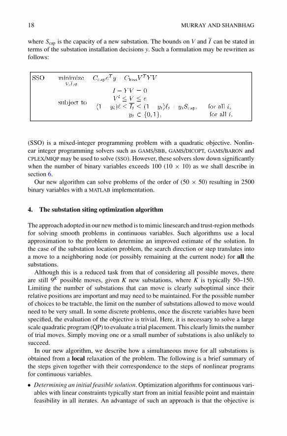
28 MURRAY AND SHANBHAG
the move, we are not concerned with whether the intermediate steps are feasible withrespect to voltage bounds.
Estimating the “Best” move. Given the relaxed solution, the sequence of substationsto move and their destimation nodes is to be determined. Each substation can either stayin its current position or can move to node c(k) on stencil k. The specification of c(k)is based on the node that has the greatest percentage of the current (not including thecenter node). An alternate specification of c(k) could be made based on the octant inwhich the center of gravity lies.
Suppose the losses of the system are denoted by F(V), where V is the vector of nodalvoltages. By assigning a substation, the resulting change in voltage may be specified as'v. The corresponding change in cost is given by
'F(V,'v) = (V + 'v)T Y (V + 'v) & V T Y V= 'vT Y (2V + 'v). (4.7)

LOCAL RELAXATION APPROACH 29
We wish to determine the index that has the least cost increase:
i = arg min'v j
{F(V + 'v j ) & F(V )} = arg min'v j
{'vTj Y (2V + 'v j )}. (4.8)
Note that these changes in voltage are not arbitrary and correspond to the solution ofY'vj = 'ivj, where ' ivj is the change in current as a result of moving all the currentto a particular node. The solution to (4.8) requires a ranking of 2K possible voltagetrajectories, based on 2K possible moves (each substation can stay in its current positionor move to candidate node c(k)). The cost increment would require solving the systemY'v = 'iv. Recall that Y is a banded positive semidefinite matrix and has bandedCholesky factors given by
Y = RT R.
The system
Y'v = 'iv,
has rank mn&1, where 'iv $ %mn . Therefore, it suffices to use only the first mn&1 rowsof Y. The resulting system is then given by:
5Y1 w
6!
"#'v1
...'vmn
$
%& =
!
"#'iv,1
...'iv,mn&1
$
%& .
Moreover, if one specifies 'vmn = 0, the system becomes:
5Y1
6!
"#'v1
...'vmn&1
$
%& =
!
"#'iv1
...'ivmn&1
$
%& ,
which may be solved by first finding the Cholesky factor of Y1, namely R1. The followinglemma exploits the fact that the Cholesky factors are banded to get a tighter bound onthe complexity of solving the load-flow equations.
Lemma 4.1. The solution to Y1'v. = 'iv. can be obtained in O(mnb2) operations,where b is the size of the band and Y1 $ %mn#mn.
Proof: The solution of this system would require a banded Cholesky factorization(O(mnb2) and two triangular factorizations (O(mnb) each) implying a total of O(mnb2)operations (see [12]). !
Since 2K different moves have to be compared when deciding between K substations,it follows that the above system has to be solved 2K times to determine the locationof the first substation. However, one has to repeat this process for each substation withsuccessively fewer substations to consider. This leads to the following result:

30 MURRAY AND SHANBHAG
Lemma 4.2. The system Y1'v. = ' iv. has to be solved K(K+1) times to move fromthe relaxed system to a K&integer solution.
Proof: This follows immediately from the identity that(K
k=1 2k = K (K + 1). !
Let us now restate the problem at each step of the assignment method.
'v" = arg min'v
{F(V + 'v) & F(V )} = arg min'v
{'vT Y (2V + 'v)}. (4.9)
The following theorem gives a polynomial bound on the number of operations requiredto either determine an improved integer solution or terminate.
Theorem 4.1. The assignment method requires O((K (K + 1))2mnb2) operations todetermine a better integer solution or terminate.
Proof: The kth step of the assignment method requires 2k calculations of the product'vT Y (2V + 'v). The calculation 'vT Y (2V + 'v) requires O(mnb2) operations,where b is the size of the band of Y. Moreover, each step also requires the solution of theload-flow equations 'iv = Y'v, which were shown to have a complexity of O(mnb).The total complexity of the assignment method can then be stated as 2.O(mnb2)+· · ·+2K .O(mnb2) = O(K (K +1)mnb2). However, the assignment method may be repeatedK (K+1)
2 times to either obtain an improved integer solution or terminate. Therefore thetotal number of operations is O((K (K + 1))2mnb2). !
The steps of a single major iteration of the assignment methodare shown inAlgorithm 2.
4.4. Adjusting the number of substations
Once a solution has been obtained for a given number of substations, we need toadjust the number to search for a lower total cost. This may be achieved by eitheradding or removing one substation. The initial feasible solution obtained by a globalrelaxation methods specifies the number of new substations. However, the initial numberof substations may not have been correct and in this section, we show how by a localsearch (by adding or removing a substation), we can determine an “optimal” number ofnew substations.
The objective function of the (SSO) problem is the sum of the cost of capital and thecost of losses. The “optimal” number of new substations is based on a trade-off betweenthe cost of losses and the cost of capital. It shall be shown that the cost of losses is amonotonically decreasing function with the number of substations. The cost of capitalis linearly related to the number of new substations.
We shall first discuss how losses change with the addition of new substations. Let L"k
denote the minimal losses based on k substations, where minss + k + maxss .
Lemma 4.3. L"k decreases strictly monotonically with increasing k.

LOCAL RELAXATION APPROACH 31
Proof: Given that the system has k substations and the minimal losses are given by L"k .
Suppose the addition of a new substation at an unoccupied load node results in lossesLk+1. Note that if no unoccupied load node exists, then the losses are already zero sinceall the loads nodes have substations placed at them. Then the addition of this substationimplies that at least some of the load at that node gets served by the new substation withzero losses. In the past, this load required dispatch from some neighboring substation.Thus there is a strict decrease in losses by the addition of a new substation or Lk+1 < L"
k .But this is merely a feasible set of locations and any optimal solution will have lossesL"
k+1 + Lk+1. Therefore, L"k monotonically decreases with increasing k. !
The objective function of (SSO) is given by: ClossV T Y V +CcapeT y, where the numberof new substations is given by eT y. Suppose we denote the number of new substations as
32 MURRAY AND SHANBHAG
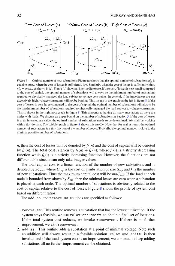
Figure 8. Optimal number of new substations: Figure (a) shows that the optimal number of substations n"ss is
equal to minss when the cost of losses is sufficiently low. Similarly, when the cost of losses is sufficiently high,n"
ss = maxss as shown in (c). Figure (b) shows an intermediate case. If the cost of losses is very small comparedto the cost of capital, the optimal number of substations will always be the minimum number of substationsrequired to physically managed the load subject to voltage constraints. In general, if the impedances are notexcessively high, voltage constraints will not be binding. This is seen in the graph on the left in figure 8. If thecost of losses is very large compared to the cost of capital, the optimal number of substations will always bethe maximum number of substations required to physically managed the load subject to voltage constraints.This is shown in the rightmost graph in figure 8. This amounts to having as many substations as there arenodes with loads. We discuss an upper bound on the number of substations in Section 5. If the cost of lossesis at an intermediate value, the optimal number of substations needs to be determined. We shall be workingwithin this domain. The middle graph in figure 8 shows this profile. Note that for real systems, the optimalnumber of substations is a tiny fraction of the number of nodes. Typically, the optimal number is close to theminimal possible number of substations.
n, then the cost of losses will be denoted by fL(n) and the cost of capital will be denotedby fC(n), The total cost is given by fL(n) + fC(n), where fL(·) is a strictly decreasingfunction while fC(·) is a strictly increasing function. However, the functions are notdifferentiable since n can only take integer values.
The total capital cost is a linear function of the number of new substations and isdenoted by kCcap, where Ccap is the cost of a substation of size Scap and k is the numberof new substations. Thus the maximum capital cost will be mnCcap. If the load at eachnode is bounded from above by Scap, then the minimal losses are zero when a substationis placed at each node. The optimal number of substations is obviously related to thecost of capital relative to the cost of losses. Figure 8 shows the profile of system costbased on different ratios.
The add-ss and remove-ss routines are specified as follows:
1. remove-ss: This routine removes a substation that has the lowest utilization. If thesystem stays feasible, we use relax-and-shift to obtain a final set of locations.If the total system cost reduces, we invoke remove-ss . If there is no furtherimprovement, we exit remove-ss .
2. add-ss: This routine adds a substation at a point of minimal voltage. Note suchan addition will always result in a feasible solution. relax-and-shift is theninvoked and if the total system cost is an improvement, we continue to keep addingsubstations till no further improvement can be obtained.
LOCAL RELAXATION APPROACH 33
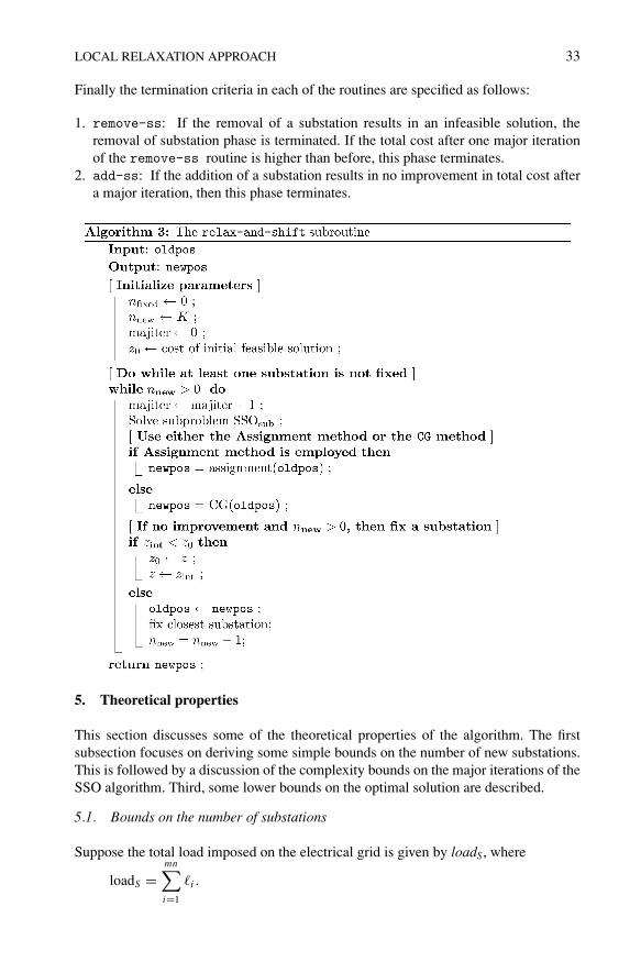
Finally the termination criteria in each of the routines are specified as follows:
1. remove-ss: If the removal of a substation results in an infeasible solution, theremoval of substation phase is terminated. If the total cost after one major iterationof the remove-ss routine is higher than before, this phase terminates.
2. add-ss: If the addition of a substation results in no improvement in total cost aftera major iteration, then this phase terminates.
5. Theoretical properties
This section discusses some of the theoretical properties of the algorithm. The firstsubsection focuses on deriving some simple bounds on the number of new substations.This is followed by a discussion of the complexity bounds on the major iterations of theSSO algorithm. Third, some lower bounds on the optimal solution are described.
5.1. Bounds on the number of substations
Suppose the total load imposed on the electrical grid is given by loadS, where
loadS =mn'
i=1
!i .
34 MURRAY AND SHANBHAG
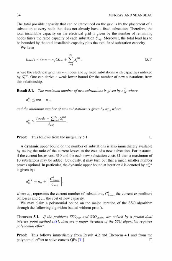
The total possible capacity that can be introduced on the grid is by the placement of asubstation at every node that does not already have a fixed substation. Therefore, thetotal installable capacity on the electrical grid is given by the number of remainingnodes times the rated capacity of each substation Scap. Moreover, the total load has tobe bounded by the total installable capacity plus the total fixed substation capacity.
We have
loadS + (mn & n f )Scap +n f'
i=1
Scapi , (5.1)
where the electrical grid has mn nodes and nf fixed substations with capacities indexedby Scap
i . One can derive a weak lower bound for the number of new substations fromthis relationship.
Result 5.1. The maximum number of new substations is given by nUss , where
nUss + mn & n f ,
and the minimum number of new substations is given by nLss , where
nLss -
loadS &(n f
i=1 Scapi
Scap.
Proof: This follows from the inequality 5.1. !
A dynamic upper bound on the number of substations is also immediately availableby taking the ratio of the current losses to the cost of a new substation. For instance,if the current losses cost $10 and the each new substation costs $1 then a maximum of10 substations may be added. Obviously, it may turn out that a much smaller numberproves optimal. In particular, the dynamic upper bound at iteration k is denoted by nU,k
ssis given by:
nU,kss = nss +
7Ck
losses
Ccap
8,
where nss represents the current number of substations, Cklosses the current expenditure
on losses and Ccap the cost of new capacity.We may claim a polynomial bound on the major iteration of the SSO algorithm
through the following algorithm (stated without proof).
Theorem 5.1. If the problems SSOsub and SSOsubint are solved by a primal-dualinterior point method [31], then every major iteration of the SSO algorithm requirespolynomial effort.
Proof: This follows immediately from Result 4.2 and Theorem 4.1 and from thepolynomial effort to solve convex QPs [31]. !
LOCAL RELAXATION APPROACH 35
5.2. Obtaining a lower bound
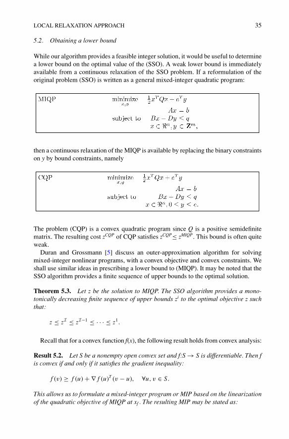
While our algorithm provides a feasible integer solution, it would be useful to determinea lower bound on the optimal value of the (SSO). A weak lower bound is immediatelyavailable from a continuous relaxation of the SSO problem. If a reformulation of theoriginal problem (SSO) is written as a general mixed-integer quadratic program:
then a continuous relaxation of the MIQP is available by replacing the binary constraintson y by bound constraints, namely
The problem (CQP) is a convex quadratic program since Q is a positive semidefinitematrix. The resulting cost zCQP of CQP satisfies zCQP+ zMIQP. This bound is often quiteweak.
Duran and Grossmann [5] discuss an outer-approximation algorithm for solvingmixed-integer nonlinear programs, with a convex objective and convex constraints. Weshall use similar ideas in prescribing a lower bound to (MIQP). It may be noted that theSSO algorithm provides a finite sequence of upper bounds to the optimal solution.
Theorem 5.3. Let z be the solution to MIQP. The SSO algorithm provides a mono-tonically decreasing finite sequence of upper bounds zi to the optimal objective z suchthat:
z + zI + zI&1 + · · · + z1.
Recall that for a convex function f(x), the following result holds from convex analysis:
Result 5.2. Let S be a nonempty open convex set and f:S ) S is differentiable. Then fis convex if and only if it satisfies the gradient inequality:
f (v) - f (u) + / f (u)T (v & u), (u, v $ S.
This allows us to formulate a mixed-integer program or MIP based on the linearizationof the quadratic objective of MIQP at xf . The resulting MIP may be stated as:

36 MURRAY AND SHANBHAG
Assumption 5.1(a) 1
2 xT Qx is bounded from above by fU.(b) (Slater’s constraint qualification): There exists a point x $ X such that Bx + Dy <
0, for each y $ Zm 0 V , where V = {y : Bx + Dy + 0 for some x $ X}.
Lemma 5.1. Given that Assumption 5.1 holds, the optimal objective zl of M is a lowerbound to the optimal objective of MIQP.
Proof: We provide an analogous proof to that in [7]. The optimal objective of MIQPis
z(x", y") : = eT y" + 12
(x")T Qx"
= min-
eT y + 12
xT Qx : Ax = b, Bx + Dy + q, x $ %n, y $ Zm9.
This problem may be reformulated as:
However, it may be seen that 0 - 12 xT Qx & µ - 1
2 xTf Qx f + xT
k Q(x & x f ) implyingthat the feasible region of M, FMIQP2FM . Therefore zl + z. !
We term (M) as a relaxed master problem. A sequence of relaxed master problemM(k) may be defined as follows:

LOCAL RELAXATION APPROACH 37
The optimal value of M(k) increases monotonically with k since the feasible region ofM(k) gets smaller due to the addition of cuts. Obviously, if at the kth iterate, the solutionobtained by the SSO algorithm is within ( of the largest lower bound (as provided bythe optimal value of M(k)), then we may claim to have an (-optimal solution.
Lemma 5.2. The optimal objective of M(k) is denoted by zk. The sequence zk ismonotone nondecreasing and zk + z for all k $ {1, . . . , I}, where I is the number ofmajor iterations of the SSO algorithm.
Proof: This follows immediately from the fact that FM(k) 1 FM(k&1) 1 · · · 1 FM(1).!
Theorem 5.4. If some member of the upper bound sequence zi is less than somemember of the lower bound sequence zk for some k, i $ {1, . . . , I}, then the solutionobtained by the SSO algorithm is optimal.
Proof: This is obvious. !
If the SSO algorithm terminates at a sub-optimal solution, then there will be a finitegap between zI and zI . At this point, neither then CG method nor the assignmentmethod is able to provide an improved integer solution. It may be possible to get furtherimprovement by using the solution of M(I) to obtain an improved solution. If one doesadopt such a strategy, the method becomes similar to the outer-approximation methodas described in [7]. However, we shall assume that such a strategy would prove uselessfor problems in which the number of integers is of the order of a few thousand.
6. Results
This section discusses some computational results. Section 6.1 specifies the platforms,operating systems and solvers used in the implementation and testing. We tested thealgorithm on three different load distributions and provide a description of each. Section6.2 compares the performance of our algorithm with that of some commercial MINLPsolvers such as DICOPT, SBB, and CPLEX. Section 6.3 gives a description of the behaviorof the SSO algorithm on some large scale problems while Section 6.4 shows the impactof changing Cmult on the optimal solution. Section 6.5 discusses the variation of thesystem cost with the number of newly installed substations. Finally, we discuss thequality of the solution in Section 6.6
6.1. Implementation details
The SSO algorithm was implemented in MATLAB 6.5 and tested on two systems:
1. A Pentium P-4 processor running WINDOWS-XP with 512 MB of RAM.2. A SunEnterprise 5500 running Solaris 8 with 4 GB of RAM.
The Tomlab [14] interface was required for using the SNOPT [10] and SQOPT [11]subroutines in MATLAB. We calibrated the results by running the problems against four

38 MURRAY AND SHANBHAG
Figure 9. Gaussian load distribution: 20 # 20 (left) and sample snohomish PUD load distribution: 24 # 46(right).
commercial solvers: CPLEX, GAMS/DICOPT, GAMS/SBB and GAMS/BARON. The algorithmswere tested on three different load distributions:
1. Uniform load distribution.2. Gaussian load distribution as shown at the left of figure 9.3. Sample load distribution from the Snohomish PUD at the right of figure 9.
6.2. Computational results from commercial solvers
This subsection shall compare the performance of three MINLP solvers with our al-gorithm. We considered the following solvers for our calibration tests: GAMS/DICOPT,GAMS/SBB and CPLEX. We restricted our load distribution to the gaussian load distribu-tion as described in the earlier section. Results for grid sizes varying from 6 # 6 to 20# 20 are given in Table 2. GAMS/DICOPT did not converge for even the smallest size andits performance shall not be reported. Table 2 reports the final costs (scaled by 1e3) andfinal number of substations for the CG and Assignment methods as obtained for thenon-uniform distribution. We report the performance of SBB and CPLEX. It should benoted that both these solvers fail to solve problems to optimality for sizes larger than 9# 9. We get suboptimal results for SBB upto 19 # 19. However, the results obtained bythem in some cases are 10% worse than the CG algorithm.
We also studied the performance of a global optimization solver GAMS/BARON fora set of problems (see Table 3). We find that except for the 6# 6 and 7 # 7 cases,GAMS/BARON never finds the optimal solution, given the limitation of 3,600 s of CPUtime.
An interesting observation that may be made with such a solver is that the performanceis affected by the underlying combinatorial problem. For instance, in the 6 # 6 case,there was exactly one substation that was finally installed and the resulting computationaltime with GAMS/BARON missing was 28 s. However, when the load was increased toa level requiring a minimum of two substations was necessary, the computational timewent up to 6 h and 34 s.

LOCAL RELAXATION APPROACH 39
Table 2. Comparison with Commercial MINLP Solvers: SBB: Note that z0 and n0 represents the costand the number of substations in the initial feasible solution. C: CPLEX, A: Assignment Method, G: CGMethod, s: SBB. z has been scaled by 1e3. Note that the results from SBB are early termination results at 1000branch-and-bound nodes. * implies failure and z* represents optimal values obtained by SBB when there isno upper bound on branch-and-bound nodes.
Initial CG Assign. SBB CPLEX
Size n0 z0 nG zG nA zA ns zs z"s nC zC
6 # 6 1 2.2 1 2.2 1 2.2 1 2.1 2.1 1 2.1
7 # 7 1 2.0 1 2.0 1 2.0 1 2.1 2.0 1 2.0
8 # 8 2 4.9 2 4.2 2 4.1 2 4.3 4.1 2 4.1
9 # 9 2 5.0 2 4.3 2 4.2 2 4.5 * 2 4.2
10 # 10 3 7.4 4 6.5 3 6.6 3 6.4 * * *
11 # 11 2 9.6 4 6.6 3 6.7 3 6.8 * * *
12 # 12 3 11.8 5 8.7 4 8.9 4 9.2 * * *
13 # 13 3 17.8 5 10.7 6 11.1 4 11.8 * * *
14 # 14 3 17.0 6 11.0 6 11.3 4 12.4 * * *
15 # 15 4 22.2 6 13.0 8 13.5 5 15.0 " " "
16 # 16 5 20.8 8 15.5 8 15.8 5 15.4 " " "
17 # 17 5 28.3 9 17.6 8 18.5 7 16.9 " " "
18 # 18 6 26.4 10 19.6 11 20.3 8 22.2 " " "
19 # 19 6 34.5 11 21.9 10 23.1 9 23.9 " " "
20 # 20 6 38.7 13 24.2 12 25.5 " " " " "
Table 3. Comparison with GAMS/BARON: In several cases, the solver terminates with a solution found inthe pre-processing phase and finds no better solution till the computational time limit expires.
Size zCG zB ARO NzBARO N
zCGCPUB ARO N
6 # 6 0.002 0.002 1.00 28
7 # 7 0.002 0.002 1.00 79
8 # 8 0.0042 0.011 2.53 3600"
9 # 9 0.0043 0.008 1.79 475
10 # 10 0.0065 0.015 2.29 387
11 # 11 0.0066 0.009 1.41 1376
12 # 12 0.0087 0.032 3.65 3600"
13 # 13 0.0107 0.020 1.84 3109
14 # 14 0.011 0.021 1.95 319
15 # 15 0.013 0.040 3.11 3600"
16 # 16 0.0155 0.029 1.89 387
17 # 17 0.0176 0.031 1.76 678
18 # 18 0.0196 0.364 18.56 3600"

40 MURRAY AND SHANBHAG
Figure 10. Comparison of scaled computational effort Cost vs. scaled number of integers. This ratio is set as1000 when the solver fails to converge or terminate gracefully. The y-axis has been drawn with a logarithmicscale.
It is observed that the SSO algorithm produces comparable optimal costs to thoseproduced by commercial solvers in the few cases that we can compare. While it is difficultto compare the computational effort of our algorithm with commercial solvers on thebasis of iterations, it is possible to construct ratios of every algorithm’s performancewith the effort taken to solve the 6 # 6 case. We show the scaled computational effortwith the scaled number of integers in figure 9.2 It can be seen that our algorithm showsmodest growth in computational effort with the number of integers. However, the twocommercial solvers show exponential growth in computational effort. In fact, for the 8# 8 case, the computational effort of SBB and CPLEX grows by factors of 39 and 62respectively. To exemplify the differences in time taken, the SSO algorithm takes lessthan a minute to solve the 15 # 15 case while CPLEX takes over 10 h (on Solaris 8).Note that CPLEX took 3.47 CPU seconds to solve the 6 # 6 problem.
6.3. Computational results on large problems
This section shall show the workings of the algorithm on sizes as large as 50 # 50. Interms of integer variables, this would be more than 25 times the largest problem thatCPLEX can handle within a reasonable period of time. We vary the grid size and use twoload distributions: a uniform (Table 5) and a gaussian (Table 4) load distributions withsizes ranging from 10 # 10 to 50 # 50. The CG method consistently produced betterresults efficiently. It may also be noticed that the two methods do not always terminatewith the same number of substations. Tables 6 and 7 show the lower bounds obtainedfor both forms of the SSO algorithm. As a comparison, the cost obtained by solvingthe convex quadratic program has also been shown. Since, the lower bounds require the

LOCAL RELAXATION APPROACH 41
Table 4. Non-uniform load distribution. Note that z0 and n0 represents the cost and the number of substationsin the initial feasible solution.
Initial CG Assign.
Size n0 z0 nG zG nA zA zconvex
10 # 10 3 0.0074 4 0.0065 3 0.0066 0.0031
15 # 15 4 0.0222 6 0.013 8 0.0135 0.0031
20 # 20 6 0.0387 13 0.0242 12 0.0255 0.0056
25 # 25 8 0.1085 20 0.0375 18 0.0388 0.0087
30 # 30 13 0.1377 26 0.0565 24 0.0585 0.0127
35 # 35 18 0.2254 37 0.0762 30 0.0824 0.0173
40 # 40 20 0.2696 46 0.0993 41 0.106 0.0224
45 # 45 26 0.3532 56 0.1278 51 0.1356 0.0285
50 # 50 34 0.4364 65 0.1605 54 0.1766 0.0350
Table 5. Uniform load distribution. Note that z0 and n0 represents the cost and the number of substationsin the initial feasible solution.
Initial CG Assign.
Size n0 z0 nG zG nA zA zconvex
10 # 10 3 0.0092 4 0.0066 4 0.0067 0.0031
15 # 15 4 0.0302 8 0.0136 8 0.0136 0.0030
20 # 20 6 0.0498 13 0.0247 14 0.0248 0.0056
25 # 25 8 0.1374 20 0.0382 20 0.0383 0.0086
30 # 30 13 0.1377 27 0.0569 26 0.0572 0.0127
35 # 35 18 0.2696 38 0.0767 36 0.0774 0.0172
40 # 40 20 0.282 46 0.1002 38 0.1068 0.0223
45 # 45 26 0.3659 57 0.1285 48 0.1371 0.0284
50 # 50 34 0.4562 74 0.1571 45 0.1979 0.0350
solution of a large mixed-integer linear program, computation of such bounds becomesdifficult for large problems.
6.4. Examining the impact of Cmult
This section examines the impact of changing Cmult on the optimal solution. Table 8considers a 15 # 15 and a 20 # 20 grid with a non-uniform load distribution. We solvethe problem with three choices of Cmult: 0.005, 0.003 and 0.001. It may be noticed thatall three settings result in very similar solutions albeit through very different paths. Thefirst starts with only 4 substations and goes on to add two more. By reducing Cmult
to 0.003 results in an initial setting at 5 substations with termination at 7 substations.Finally, if we set Cmult at 0.001, the initial feasible solution starts at 7 substations and
42 MURRAY AND SHANBHAG
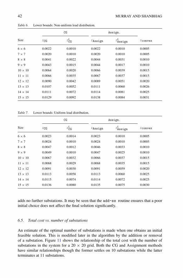
Table 6. Lower bounds: Non-uniform load distribution.
CG Assign.
Size zCG zLCG zAssign zL
Assign zconvex
6 # 6 0.0022 0.0010 0.0022 0.0010 0.0005
7 # 7 0.0020 0.0010 0.0020 0.0010 0.0005
8 # 8 0.0041 0.0022 0.0044 0.0031 0.0010
9 # 9 0.0043 0.0015 0.0044 0.0017 0.0010
10 # 10 0.0064 0.0020 0.0066 0.0039 0.0015
11 # 11 0.0066 0.0035 0.0067 0.0037 0.0015
12 # 12 0.0090 0.0042 0.0089 0.0051 0.0020
13 # 13 0.0107 0.0052 0.0111 0.0060 0.0026
14 # 14 0.0111 0.0072 0.0114 0.0081 0.0025
15 # 15 0.0129 0.0092 0.0138 0.0084 0.0031
Table 7. Lower bounds: Uniform load distribution.
CG Assign.
Size zCG zLCG zAssign zL
Assign zconvex
6 # 6 0.0023 0.0014 0.0023 0.0010 0.0005
7 # 7 0.0024 0.0010 0.0024 0.0010 0.0005
8 # 8 0.0047 0.0012 0.0046 0.0033 0.0010
9 # 9 0.0049 0.0010 0.0047 0.0025 0.0010
10 # 10 0.0067 0.0032 0.0066 0.0037 0.0015
11 # 11 0.0068 0.0029 0.0068 0.0035 0.0015
12 # 12 0.0091 0.0030 0.0091 0.0059 0.0020
13 # 13 0.0113 0.0058 0.0113 0.0060 0.0025
14 # 14 0.0115 0.0074 0.0114 0.0072 0.0025
15 # 15 0.0136 0.0080 0.0135 0.0075 0.0030
adds no further substations. It may be seen that the add-ss routine ensures that a poorinitial choice does not affect the final solution significantly.
6.5. Total cost vs. number of substations
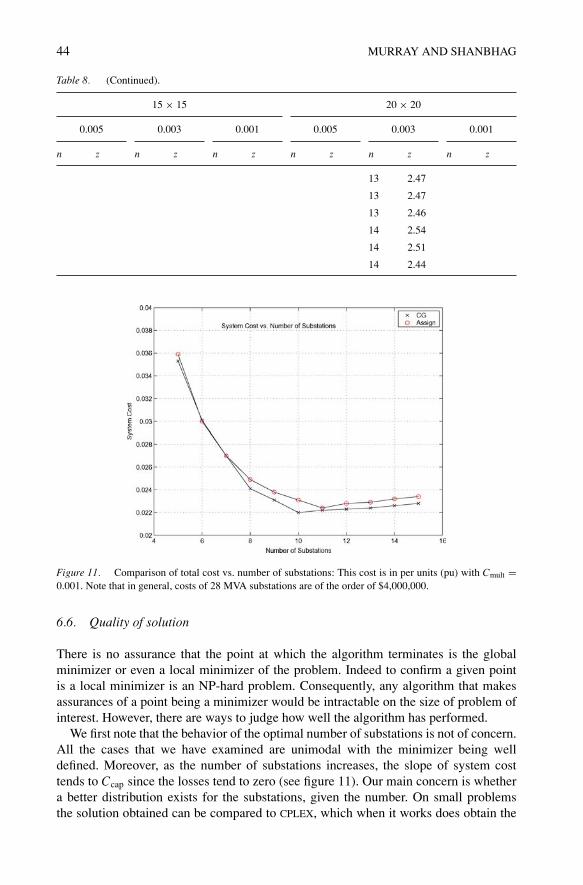
An estimate of the optimal number of substations is made when one obtains an initialfeasible solution. This is modified later in the algorithm by the addition or removalof a substation. Figure 11 shows the relationship of the total cost with the number ofsubstations in the system for a 20 # 20 grid. Both the CG and Assignment methodshave similar relationships though the former settles on 10 substations while the latterterminates at 11 substations.

LOCAL RELAXATION APPROACH 43
Table 8. Impact of changing Cmult on solution for a 15 # 15 and a (20 # 20) grid.
15 # 15 20 # 20
0.005 0.003 0.001 0.005 0.003 0.001
n z n z n z n z n z n z
4 2.22 5 1.84 7 1.46 6 3.87 7 3.76 8 3.65
4 1.81 5 1.58 7 1.39 6 3.60 7 3.38 8 3.20
4 1.72 5 1.55 7 1.39 7 3.31 7 3.34 8 3.15
5 1.63 5 1.50 7 1.38 7 3.13 7 3.29 8 3.05
5 1.61 5 1.49 7 1.36 7 3.08 7 3.26 8 3.04
5 1.55 6 1.47 7 1.36 7 3.04 7 3.25 8 2.95
5 1.53 6 1.41 7 1.36 7 2.99 8 3.18 8 2.94
5 1.49 6 1.40 7 1.35 8 2.94 8 3.11 8 2.91
5 1.47 7 1.38 7 1.34 8 2.82 8 3.08 8 2.88
5 1.44 7 1.34 7 1.33 8 2.81 8 3.07 8 2.88
5 1.43 7 1.30 9 2.83 8 3.03 8 2.83
5 1.40 7 1.30 9 2.66 8 3.00 9 2.79
5 1.40 10 2.62 8 3.00 9 2.71
6 1.37 10 2.60 8 2.99 9 2.68
6 1.33 10 2.55 8 2.96 9 2.64
6 1.33 10 2.52 8 2.96 10 2.68
6 1.30 11 2.50 8 2.93 10 2.60
11 2.49 8 2.92 10 2.56
11 2.49 8 2.90 10 2.54
12 2.55 9 2.78 10 2.53
12 2.46 9 2.72 11 2.56
12 2.45 9 2.70 11 2.53
13 2.53 9 2.69 11 2.53
13 2.47 10 2.66 11 2.52
13 2.42 10 2.64 11 2.52
13 2.42 10 2.62 11 2.50
10 2.61 12 2.50
10 2.61 12 2.45
11 2.61 12 2.45
11 2.49
11 2.49
12 2.56
12 2.46
13 2.51
Continued on next page.
44 MURRAY AND SHANBHAG
Table 8. (Continued).
15 # 15 20 # 20
0.005 0.003 0.001 0.005 0.003 0.001
n z n z n z n z n z n z
13 2.47
13 2.47
13 2.46
14 2.54
14 2.51
14 2.44
Figure 11. Comparison of total cost vs. number of substations: This cost is in per units (pu) with Cmult =0.001. Note that in general, costs of 28 MVA substations are of the order of $4,000,000.
6.6. Quality of solution
There is no assurance that the point at which the algorithm terminates is the globalminimizer or even a local minimizer of the problem. Indeed to confirm a given pointis a local minimizer is an NP-hard problem. Consequently, any algorithm that makesassurances of a point being a minimizer would be intractable on the size of problem ofinterest. However, there are ways to judge how well the algorithm has performed.
We first note that the behavior of the optimal number of substations is not of concern.All the cases that we have examined are unimodal with the minimizer being welldefined. Moreover, as the number of substations increases, the slope of system costtends to Ccap since the losses tend to zero (see figure 11). Our main concern is whethera better distribution exists for the substations, given the number. On small problemsthe solution obtained can be compared to CPLEX, which when it works does obtain the

LOCAL RELAXATION APPROACH 45
Figure 12. Effect of starting points: Clockwise from top left: (i) Symmetric initial placement with cost =0.0166 and final costs 0.0113 (CG) and 0.0117 (Assignment) (ii) Poor initial placement with cost = 0.0316 andfinal costs 0.0113 (CG) and 0.0118 (Assignment) (iii) Good placement as specified by the solution on SSOsontwith cost = 0.0125 and final costs given by 0.0113 (CG) and 0.0115 (Assignment) (iv) Load distribution. Notethat “x” and “"” refer to the initial and final positions while the triangles denote the intermediate positions.
correct solution. However, in the case of small problems a substation being displacedby one node results in a significant relative error in cost since there are only one ortwo substations. In practice a displacement of one node is of little significance. Recallthat we are identifying which blocks to place the substation and where in the block isdecided later. It could be at a boundary and hence be very similar to a solution in whichthe substation is placed in the adjacent block. In all the tests the biggest difference indisplacement was one substation being out by one node. The relative difference in costwas around 1%.
By choosing special load distributions, the solution can be inferred from geometricarguments. For example, given a uniform load and say four substations we would expectthe placement of the substations to symmetric. Again in all the tests on such problemsthe termination point was symmetric or at most one node displaced with the relativecost being very close to the minimum cost. Figure 13 shows the load distribution, whena four gaussian loads are placed in the centers of the four quadrants.
We can also check whether or not we converge to the same or similar terminationpoints if we start from different initial points. Since we have a procedure to determine
46 MURRAY AND SHANBHAG
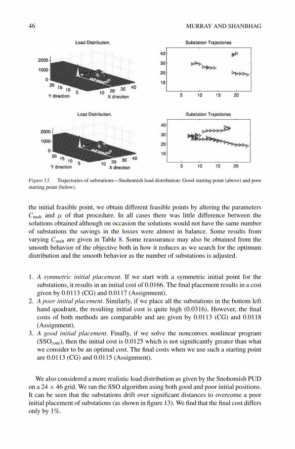
Figure 13. Trajectories of substations—Snohomish load distribution: Good starting point (above) and poorstarting point (below).
the initial feasible point, we obtain different feasible points by altering the parametersCmult and µ of that procedure. In all cases there was little difference between thesolutions obtained although on occasion the solutions would not have the same numberof substations the savings in the losses were almost in balance. Some results fromvarying Cmult are given in Table 8. Some reassurance may also be obtained from thesmooth behavior of the objective both in how it reduces as we search for the optimumdistribution and the smooth behavior as the number of substations is adjusted.
1. A symmetric initial placement. If we start with a symmetric initial point for thesubstations, it results in an initial cost of 0.0166. The final placement results in a costgiven by 0.0113 (CG) and 0.0117 (Assignment).
2. A poor initial placement. Similarly, if we place all the substations in the bottom lefthand quadrant, the resulting initial cost is quite high (0.0316). However, the finalcosts of both methods are comparable and are given by 0.0113 (CG) and 0.0118(Assignment).
3. A good initial placement. Finally, if we solve the nonconvex nonlinear program(SSOcont), then the initial cost is 0.0125 which is not significantly greater than whatwe consider to be an optimal cost. The final costs when we use such a starting pointare 0.0113 (CG) and 0.0115 (Assignment).
We also considered a more realistic load distribution as given by the Snohomish PUDon a 24 # 46 grid. We ran the SSO algorithm using both good and poor initial positions.It can be seen that the substations drift over significant distances to overcome a poorinitial placement of substations (as shown in figure 13). We find that the final cost differsonly by 1%.

LOCAL RELAXATION APPROACH 47
7. Conclusions and future work
We consider a grid-based location problem with quadratic costs and linear constraints.We have proposed a new method for locating substations in such a grid. The proposedalgorithm solves a quadratic program to obtain a direction of descent. Two differentmethods are proposed for determining an appropriate step. Both methods despite beingmarkedly different, produced similar results. Of the two methods, the CG method con-sistently produced better results efficiently. The number of substations is also optimizedby adding and removing substations until no further improvement can be obtained.
Bounds have been provided on the computational effort for a major iteration. Both setsof bounds depend on the square of the total number of substations. In practice, howeversuch a growth has not been observed. It is also seen that the size of the continuousquadratic subproblem is not affected by the number of substations. Results have beenprovided for cases up to 2500 integers (50 # 50) and larger cases have also been solved.Comparable results on general purpose nonlinear integer programming solvers have alsobeen provided. For cases larger than 81 integer variables, these solvers fail. The growthin effort with the number of integers is slow with the proposed algorithm. However, forthe commercial solvers, this growth is observed to be exponential.
The efficiency of the CG method could be improved by taking a less conservativestrategy in the choice of ". As we have noted earlier, we can fix more than one substationat a time when we are unable to find an improved solution immediately. We could alsowarm-start the QP subproblem or use a more sophisticated search for the number ofsubstations. To date, none of these steps have proved necessary.
There is little, if at all, in theory to deal with more complex nonlinear grid-basedfacility location problems. Our method may be extended to general nonlinear costfunctions by using a general NLP solver (such as SNOPT) instead of a QP solver.Alternately, we may also use a local QP approximation of the nonlinear problem.
The problem as posed may be embellished in a number of ways. For example, thesize of substations can be varied among a discrete set or the transmission lines may beupgraded to specified levels. Such enhancements add to the size and complexity of themodel but do not alter its form. To be able to solve such problems clearly requires thatwe solve the current problem quickly. This has been achieved by our new algorithm.
Acknowledgments
We extend our sincere thanks to Robert H. Fletcher, Public Utility District No. 1 ofSnohomish County, Everett, Washington and Patrick Gaffney, Bergen Software ServicesInternational (BSSI), for their guidance and support. This research was supported byOffice of Naval Research grant N00014-02-1-0076 and National Science Foundation.
Note
1. The current (voltage) is unknown at substation (non-substation) locations
2. We do not include GAMS/BARON in this comparison since there are only two points in which the optimal
solution is obtained.

48 MURRAY AND SHANBHAG
References
1.OQNP and MSDLP, User’s Manual, Optimal Methods Inc. and OptTek System Inc.2.R.N. Adams and M.A. Laughton, Static and time phased network synthesis, Proc. IEE, vol. 121, pp. 139–147,
1974.3.R.K. Ahuja, T.L. Magnanti, and J.B. Orlin, Network Flows: Theory, Algorithms and Applications, Prentice
Hall: Englewood Cliffs, NJ, 1993.4.H.M. Amir and T. Hasegawa, “Nonlinear mixed-discrete structural optimization,” Journal of Structural
Engineering, vol. 115, pp. 626–646, 1989.5.J.Z. Cha and R.W. Mayne, “Optimization with discrete variables via recursive quadratic programming:
Part 2 - algorithms and results,” Transactions of the ASME, Journal of Mechanisms, Transmissions andAutomation in Design, vol. 111, pp. 130–136, 1989.
6.D.M. Crawford and S.B. Holt, “A mathematical optimization technique for locating and sizing distributionsubstations and deriving their optimal service areas,” IEEE Transactions on PAS, pp. 230–235, 1975.
7.M. Duran and I. Grossmann, “An outer-approximation algorithm for a class of mixed-integer nonlinearprograms,” Mathematical Programming, vol. 36, pp. 307–339, 1986.
8.M.A. El-Kady, “Computer-aided planning of distribution substation and primary feeders,” IEEE Transac-tions on PAS, vol. PAS-103, pp. 1183–1192, 1984.
9.A.M. Geoffrion, “Generalized benders decomposition,” J. Optim. Theory Appl,, vol. 10, pp. 237–260, 1972.10.P.E. Gill, W. Murray, and M.A. Saunders, SNOPT: An SQP algorithm for large-scale constrained opti-
mization, Tech. Report NA–97–2, Systems Optimization Laboratory, Stanford University, San Diego, CA,1997.
11.User’s guide for SQOPT 5.3: A Fortan package for large-scale linear and quadratic programming, tech.report, Systems Optimization Laboratory, Department of Operations Research, Stanford University - 94305-4022, 1997.
12.G.H. Golub and C.F. Vanloan, “Unsymmetric positive definite linear systems,” Linear Algebra and ItsApplications, vol. 28 pp. 85–98, 1979.
13.K.S. Hindi and A. Brameller, “Design of low-voltage distribution networks: a mathematical programmingmethod,” Proc. IEE, vol. 124, pp. 54–58. 1977.
14.K. Holmstrom, “The TOMLAB Optimization Environment in Matlab,” Advanced Modeling and Opti-mization, vol. 1, pp. 47–69. 1999.
15.U.G.W. Knight, “The logical design of electricity networks using linear programming methods,” Proc.IEE, vol. 117, pp. 2117–2127. 1970.
16.S. Leyffer, Deterministic Methods for Mixed Integer Nonlinear Programming, PhD thesis, University ofDundee, Dundee, Scotland, UK, 1993.
17.A.C. Marshall, T.B. Boffy, J.R. Green, and H. Hague, “Optimal design of electricity networks,” IEEEProceedings-C, vol. 138, pp. 69–77. 1991.
18.E. Masud, “An interactive procedure for sizing and timing distribution substations using optimizationtechniques,” IEEE Trans. on PAS, vol. 93, pp. 1281–1286. 1974.
19.J.J. More and S.J. Wright, Optimization software guide, part 2, pp 87–89, SIAM Philadelphia, 1993.20.G.L. Nemhauser and L.A. Wolsey, “Integer and Combinatorial Optimization,” John Wiley, New York,
1988.21.A. Neumaier, O. Shcherbina, W. Huyer, and T. Vinko, “A comparison of complete global optimization
solvers,” Mathematical Programming, Series B., vol. 103, pp. 333–356. 2004.22.K.-M. Ng, A Continuation Approach to Solving Continuous Problems with Discrete Variables, PhD thesis,
Stanford University, Stanford, CA 94305, June, 2002.23.G.R. Olsen and G.N. Vanderplaats, “Methods for nonlinear optimization with discrete design variables,”
AIAA Journal, vol. 27, pp. 1584–1589, 1989.24.N.V. Sahinidis and M. Tawarmalani, “Baron 7.2: Global Optimization of Mixed-Integer Nonlinear Pro-
grams,” User’s Manual, 2004.25.S. Sharif, M. Salamat, and A. Vanelli, “Model for future expansion of radial distribution networks using
mixed integer programming,” IEEE, pp. 152–155, 1996.26.M. Tawarmalani and N.V. Sahinidis, “Global optimization of mixed-integer nonlinear programs: A theo-
retical and computational study,” Mathematical Programming, vol. 99, pp. 563–591. 2004.27.G.L. Thompson and D.L. Wall, “A branch and bound model for choosing optimal substation locations,”

LOCAL RELAXATION APPROACH 49
IEEE Transactions on PAS,, PAS-100 pp. 2683–2687, 1981.28.D.L. Wall, G.L. Thompson, and J.E.D. Northcote-Green, “An optimization model for planning radial
distribution networks,” IEEE Transactions on PAS, PAS-98 pp. 1061–1066. 1979.29.H.L. Willis, H. Tram, M.V. Engel, and L. Finley, “Optimization applications to distribution,” IEEE Com-
puter Applications in Power, vol. 10, pp. 12–17, 1995.30.H.L. Willis, H. Tram, M.V. Engel and L. Finley, “Selecting and applying distribution optimization methods,”
IEEE Computer Applications in Power, vol. 1, pp. 12–17, 1996.31.S.J. Wright, Primal-Dual Interior-Point Methods, SIAM, 1996.32.K. Yahav and G. Oron, “Optimal locations of electrical substations in regional energy supply systems,”
IEEE, pp. 307–310, 1996.