A kinetic scheme for transient mixed ﬂows in non uniform

A kinetic scheme for transient mixed flows in

non uniform closed pipes: a global manner to

upwind all the source terms

C. Bourdarias∗, M. Ersoy†‡, S. Gerbi§

Universite de Savoie, Laboratoire de Mathematiques,

73376 Le Bourget-du-Lac Cedex, France.

November 22, 2010

Abstract

We present a numerical kinetic scheme for an unsteady mixedpressurized and free surface model. This model has a source termdepending on both the space variable and the unknown U of thesystem. Using the Finite Volume and Kinetic (FVK) framework, wepropose an approximation of the source terms following the principleof interfacial upwind with a kinetic interpretation. Then, severalnumerical tests are presented.

Keywords : Finite volume scheme, Kinetic scheme, Conservative sourceterms, Non-conservative source terms, Friction

1 Introduction

In this paper, we study a way to upwind the source terms of a mixed flowsmodel in non uniform closed water pipes in a one dimensional framework.In the case of free surface incompressible flows, the model is called FS-model and it is an extension of classical Saint-Venant models. When thepipe is full, we introduce the pressurized model, called P-model, whichdescribes the evolution of a compressible inviscid flow and is close to gas

∗[email protected]†[email protected]‡BCAM - Basque Center for Applied Mathematics, Bizkaia Technology Park 500,

48160, Derio, Basque Country, Spain§[email protected]

1

dynamics equations in a nozzle. In order to cope with the transition be-tween a free surface and a pressurized model, we use a mixed model calledPFS-model. It is based on balance laws and provides an hyperbolic systemwith source terms corresponding to the inclination of the pipe (seen as atopography term), the section variation, the curvature and the friction.

Several ways to compute the numerical approximation of conservationlaws with source terms have already been investigated by many authors.The main difficulty is to preserve numerically some properties satisfied bythe continuous model: the invariant domain and the well-balanced propertyfor instance. The Finite Volume methods are largely used since they presentthe remarkable property to be domain invariant (for instance, for Saint-Venant equations, to be water height conservative). Some Well-BalancedFinite Volume schemes, introduced by Greenberg et al [5], preserve steadystates. All these methods are based on two principles: firstly, the con-servative quantities are cell-centered as usual finite volume schemes, andsecondly the source terms are upwinded at the cell interfaces.

In this paper, we consider a particular Finite Volume-Kinetic schemebuilt to compute the numerical solution of the PFS-model. This schemeis based on the classical kinetic interpretation [6] of the system.

The source terms appearing in the PFS-model are either conserva-tive, non-conservative or else. All source terms are upwinded at the cellinterfaces: we use the definition of the DLM theory [3] to define the non-conservative products. The particular case of the friction term which isneither conservative nor non-conservative will be upwinded using the no-tion of dynamic slope, already introduced in [2]. The source terms are takeninto account in the numerical fluxes and are computed from the microscopicones, obtained through the concept of potential barrier.

The paper is organized as follows. In the second section, we describethe PFS-model and focus on the source terms. The detailed descriptionof the method used to deal with the transition points (when a change ofstate occurs) is not presented (see [2] or [4] for more details on this topic).We state some theoretical properties of the system. In the third section,we give the kinetic formulation of the PFS-model and the correspondingkinetic scheme. In the fourth and last section, several numerical tests areprovided.

Notations concerning geometrical quantities

• θ(x): angle of the inclination of the main pipe axis z = Z(x) at position x

• Ω(x) = S(x): cross-section area of the pipe orthogonal to the axis z = Z(x)

• R(x): radius of the cross-section S(x) orthogonal to the axis z = Z(x)

• Ω(t, x) : free surface cross-section area orthogonal to the axis z = Z(x)

• σ(x, z): width of the cross-section Ω at position x and altitude z

2

Notations concerning the PFS-model

• p(t, x, y, z): pressure

• ρ0: density of the water at atmospheric pressure p0

• ρ(t, x, y, z): density of the water at the current pressure

• ρ(t, x) =1

S(x)

∫Ω(x)

ρ(t, x, y, z) dy dz: mean value of ρ over Ω(x)

• c: sonic speed

• A(t, x) =ρ(t, x)

ρ0S(x): equivalent wet area

• u(t, x): velocity

• Q(t, x) = A(t, x)u(t, x): discharge

• E: state indicator equal to E = 0 if the flow is free surface, E = 1 otherwise

• S: the physical wet area equal to A if the state is free surface, S otherwise

• H(S): the Z-coordinate of the water level equal to H(S) = h(t, x) if thestate is free surface, R(x) otherwise

• p(x,A,E): mean pressure over Ω

• Ks > 0: Strickler coefficient depending on the material

• Pm(A): wet perimeter of A (length of the part of the channels section incontact with the water)

• Rh(A) =A

Pm(A): hydraulic radius

• Bold characters are used for vectors, except for S

2 A model for unsteady water flows in pipes

The PFS-model (see [2] or [4]) is a mixed model of a pressurized (com-pressible) and free surface (incompressible) flow in a one dimensional rigidpipe with variable cross-section. The pressurized parts of the flow corre-spond to a full pipe whereas the section is not completely filled for the freesurface flow. The Free Surface part of the model is derived by writing the3D Euler incompressible equations and by averaging over orthogonal sec-tions to the privileged axis of the flow. In the same spirit, by writing theEuler isentropic and compressible equations with the linearized pressure

law p(t, x, y, z) = p0 +1

c2(ρ(t, x, y, z)− ρ0), we obtain a Saint-Venant like

system of equations in the “FS-equivalent” variable A(t, x) =ρ(t, x)

ρ0S(x),

Q(t, x) = A(t, x)u(t, x) which takes into account the compressible effects(for a detailed derivation, see [2] or [4]).

3

In order to deal with the transition points (that is, when a change ofstate occurs), we introduce a state indicator variable E which is equal to1 if the state is pressurized and to 0 if the state is free surface. We definethe physical wet area by:

S = S(A,E) =

S if E = 1,A if E = 0.

The pressure law is given by a mixed “hydrostatic” (for the free surfacepart of the flow) and “acoustic” type (for the pressurized part of the flow)as follows:

p(x,A,E) = c2(A− S) + gI1(x,S) cos θ (1)

where g is the gravity constant, c the sonic speed of the water (assumed tobe constant) and θ the inclination of the pipe. The term I1 is the classicalhydrostatic pressure:

I1(x,S) =

∫ H(S)

−R

(H(S)− z)σ dz

where σ(x, z) is the width of the cross-section, R = R(x) the radius of thecross-section and H(S) is the z-coordinate of the free surface over the mainaxis Z(x).The defined pressure (1) is continuous throughout the transition points andwe define the PFS-model by:

∂t(A) + ∂x(Q) = 0

∂t(Q) + ∂x

(Q2

A+ p(x,A,E)

)

= −g AZ ′ + Pr(x,A,E)

−G(x,A,E)

−K(x,A,E)Q|Q|A

(2)

where z = Z(x) is the altitude of the main pipe axis. The terms Pr, Gand K denote respectively the pressure source term, a curvature term andthe friction:

Pr(x,A,E) = c2(A

S− 1

)

S′ + g I2(x,S) cos θ,

G(x,A,E) = g AZ(x,S) = g A (H(S)− I1(x,S)/S) (cos θ)′,

K(x,A,E) =1

K2sRh(S)4/3

where we have used the notation f ′ to denote the derivative with respectto the space variable x of any function f(x). The term I2 is the hydrostatic

4

pressure source term defined by: I2(x,S) =

∫ H(S)

−R

(H(S) − z)∂xσ dz . The

term Ks > 0 is the Strickler coefficient depending on the material andRh(S) is the hydraulic radius.

Identification of source terms.In order to write the kinetic formulation of the PFS equations, we have tofactorize by A the right hand side of Equation (2). Then, the source termsreads as follows:

• gZ ′ is a conservative term.

• c2(A− S

AS

)

S′ =

c2

(A−SAS

)S′ ifE = 1

0 ifE = 0is a non-conservative prod-

uct.

• gI2(x,S) cos θ

Ais a non-conservative product (since I2 could be writ-

ten as γ(x,S)S′ for some function γ specific to geometry of the pipe).

• g (H(S)− I1(x,S)/S) cos θ′ is a non-conservative product.

• K(x,A,E)Q|Q|A2

is neither conservative nor non-conservative.

Moreover, all the term said to be non-conservative product are genuinelynon-conservative product since they do not admit an exact differential form.

Figure 1: Geometric characteristics of the domainfree surface and pressurised flow

5

The System (2) has the following properties:

Theorem 2.1

1. System (2) is strictly hyperbolic on A(t, x) > 0 .

2. For smooth solutions, the mean velocity u = Q/A satisfies

∂tu+ ∂x

(u2

2+ c2 ln(A/S) + gH(S) cos θ + gZ

)

= −gK(x,A,E)u|u| 6 0.(3)

3. The still water steady state, for u = 0, reads:

c2 ln(A/S) + gH(S) cos θ + gZ = cte (4)

for some constant cte.

4. System (2) admits a mathematical entropy

E(A,Q,E) =Q2

2A+ c2A ln(A/S) + c2S + gAZ(x,S) cos θ + gAZ

which satisfies the entropy relation for smooth solutions

∂tE + ∂x((E + p(x,A,E))U

)= −gAK(x,A,E)u2|u| 6 0 . (5)

In what follows, when no confusion is possible, the term K(x,A,E) willbe noted simply K(x,A) for free surface states and K(x, S) for pressurizedstates.

Remark 2.1 The equation (4) is the still water steady state equation as-sociated to the PFS equation. It translate the fact that, when u = 0 andA = A(x), the following equations holds:

c2 ln(A/S) + gR cos θ + gZ = cte

if S = S (i.e. for a pressurized flow) and

gH(A) cos θ + gZ = cte

when S = A, i.e. the horizontal line for free surface still water steadystates. Moreover, when mixed still water steady states occur, i.e. whenone part of the flow is pressurized and the other part of the flow is freesurface, Equation (4) holds again.

6

3 The Kinetic approach

The kinetic formulation (3.1) is a (non physical) microscopic description ofthe PFS-model provided by a given real function χ : R → R satisfying thefollowing properties:

χ(ω) = χ(−ω) > 0 ,

∫

R

χ(ω)dω = 1,

∫

R

ω2χ(ω)dω = 1.

It permits to define the density of particles, by a so-calledGibbs equilibrium,

M(t, x, ξ) =A(t, x)

b(t, x)χ

(ξ − u(t, x)

b(t, x)

)

where b(t, x) = b(x,A(t, x), E(t, x))

with

b(x,A,E) =

√

gI1(x,A)

Acos θ if E = 0,

√

gI1(x, S)

Acos θ + c2 if E = 1.

3.1 The mathematical kinetic formulation

The Gibbs equilibrium M is related to the PFS-model by the classicalmacro-microscopic kinetic relations:

A =

∫

R

M(t, x, ξ) dξ , (6)

Q =

∫

R

ξM(t, x, ξ) dξ , (7)

Q2

A+Ab(x,A,E)2 =

∫

R

ξ2M(t, x, ξ) dξ . (8)

From the relations (6)–(8), the non-linear PFS-model can be viewed as asingle linear equation involving the non-linear quantity M:

Theorem 3.1 (Kinetic Formulation of the PFS-model) (A,Q) is astrong solution of System (2) if and only if M satisfies the kinetic transportequation:

∂tM+ ξ · ∂xM− gφ ∂ξM = K(t, x, ξ) (9)

for a collision term K(t, x, ξ) which satisfies for (t, x) a.e.

∫

R

(1ξ

)

K(t, x, ξ) dξ = 0.

7

The source terms are defined as:

φ(x,W) = B(x,W) · ∂xW (10)

with

W =

(

Z +

∫

x

K(x,A)u|u| dx, S, cos θ)

(11)

and B =

(

1, −c2

g

(A− S

AS

)

− γ(x, S) cos θ

A, Z(x, S)

)

if E = 1,(

1, −γ(x,A) cos θ

A, Z(x,A)

)

if E = 0

where I2(x,S) reads γ(x,S)S′ for some function γ (depending on the ge-ometry of the pipe).

We call the termd

dx

(

Z +

∫

x

K(x,A)u|u| dx)

the dynamic slope since

it is time and space variable dependent (see also [2]).

3.2 The kinetic scheme

Based on the above kinetic formulation (9), we construct easily a FiniteVolume scheme where the source terms are upwinded by a generalizedkinetic scheme with reflections [6].

To this end, let us consider a uniform mesh on R where cells are denoted

for every i ∈ Z by mi = (xi−1/2, xi+1/2), with xi =xi−1/2 + xi+1/2

2and

∆x = xi+1/2 − xi+1/2 the space-step. We consider a time discretizationtn defined by tn+1 = tn + ∆tn with ∆tn the time-step. We note Un

i =

(Ani , Q

ni ), u

ni =

Qni

Ani

, Mni the cell-centered approximation of U = (A,Q), u

and M on the cell mi at time tn.

If W is

(

Z +

∫

x

K(x,A)u|u| dx, S, cos θ)

, its piecewise constant rep-

resentation is given by, W(t, x) = Wi(t)1mi(x) where Wi(t) is defined as

Wi(t) =1

∆x

∫

mi

W(t, x) dx for instance.

Denoting by Wi and Wi+1 the left and the right states of the cell interfacexi+1/2, and using the “straight lines” paths (see [3])

Ψ(s,Wi,Wi+1) = sWi+1 + (1− s)Wi, s ∈ [0, 1],

we define the non-conservative product φ(t, xi+1/2) by writing:

[W] (t) ·∫ 1

0

B (t,Ψ(s,Wi(t),Wi+1(t))) ds (12)

8

where [W] (t) := Wi+1(t) − Wi(t), is the jump of W(t) across the dis-continuity localized at x = xi+1/2. As the first component of B is 1, werecover the classical interfacial upwinding for the term Z (appearing e.g.in Saint-Venant equations) since it is a conservative term.

Neglecting the collision kernel [6] and using the fact that φ = 0 on thecell mi (since [W] ≡ 0), the kinetic transport equation (9) simply reads:

∂

∂tf + ξ · ∂

∂xf = 0

f(tn, x, ξ) = M(tn, x, ξ)

, (t, x, ξ) ∈ [tn, tn+1)×mi × R (13)

and thus it may be discretized as follows:

fn+1i (ξ) = Mn

i (ξ) +∆tn

∆xξ (M−

i+ 12

(ξ) −M+i− 1

2

(ξ)) (14)

where the contribution of the source term is included into the microscopicnumerical fluxes M±

i±1/2. This is the principle of interfacial source upwind.

Using the macro-microscopic relations (6)–(8) and integrating Equation(14) against ξ and ξ2, we obtain the Finite Volume scheme:

Un+1i = Un

i +∆tn

∆x

(

F−i+ 1

2

− F+i− 1

2

)

(15)

where the numerical fluxes are computed by :

F±i+ 1

2

=

∫

R

(ξξ2

)

M±i+ 1

2

(ξ) dξ . (16)

Following [6] (or [1]), the microscopic fluxes are given by:

M−i+1/2(ξ) =

positive transmission︷︸︸︷

1ξ>0Mni (ξ) +

reflection︷︸︸︷

1ξ<0,ξ2−2g∆φni+1/2

<0Mni (−ξ)

+ 1ξ<0,ξ2−2g∆φni+1/2

>0Mni+1

(

−√

ξ2 − 2g∆φni+1/2

)

︸︷︷︸

negative transmission

,

M+i+1/2(ξ) =

negative transmission︷︸︸︷

1ξ<0Mni+1(ξ) +

reflection︷︸︸︷

1ξ>0,ξ2+2g∆φni+1/2

<0Mni+1(−ξ)

+ 1ξ>0,ξ2+2g∆φni+1/2

>0Mni

(√

ξ2 + 2g∆φni+1/2

)

︸︷︷︸

positive transmission

.

(17)The term ∆φn

i±1/2 in (17) is the upwinded source term (10). It also plays

the role of the potential barrier: the term ξ2 ± 2g∆φni+1/2 is the jump

condition for a particle with a kinetic speed ξ which is necessary to

9

• be reflected: this means that the particle has not enough kineticenergy ξ2/2 to overpass the potential barrier (reflection in (17)),

• overpass the potential barrier with a positive speed (positive trans-mission in (17)),

• overpass the potential barrier with a negative speed (negative trans-mission in (17)).

Taking an approximation of the non-conservative product φ (12), the po-tential barrier ∆φn

i+1/2 has the following expression:

∆φni+1/2 = [W] (tn) ·B

(

tn,Ψ

(1

2,Wi(tn),Wi+1(tn)

))

(18)

Next, with the simplest choice of the χ-function χ(ω) =1

2√31[−

√3,√3](ω),

which allows to compute easily numerical fluxes, we have:

Theorem 3.2

1. (Invariant domain) Under the CFL condition

∆tn

∆xmaxi∈Z

(

|uni |+

√3c)

< 1,

the kinetic scheme (15)–(17) keeps A positive, i.e. Ani > 0 if it is

initially true.

2. The kinetic scheme (15)–(17) allows to compute the drying and flood-ing area.

Remark 3.1 In its actual form, the numerical scheme (15)–(17) is notexactly well-balanced (in the sens of [2]: roughly speaking, for large enoughtime tn, the difference F−

i+ 12

− F+i− 1

2

in Equation (15) does not vanishes).

This drawback is due to the choice of the χ-function above.Actually, up to our knowledge, the only possible choice which allows to

construct free surface still water steady states preserving schemes (see [4])is

M =A

πb(t, x)

√

1− (ξ − u)2

4b(t, x)2

and

M =A√2πc

exp

(

− (ξ − u)2

2c2

)

for pressurized one (see [1]).

10

The first formula is only valid for pipe with uniform rectangular sectionswhile the second one holds for every geometry but the support of the χ-function is not compact: consequently a CFL condition could not be derived(see [6] for more details).

Moreover, for more general geometric configuration, Ersoy [4] showsthat the procedure described by Perthame et al. [6] to get such a χ-functionfails. Actually, there does not exist a way to find it from the microscopiclevel.

Therefore, the author in [4] propose to revisiting the definition of themacroscopic numerical fluxes, appearing in Equation (15), to overpass thisdrawback. The general result obtained is then: for every arbitrary χ-function, the numerical scheme (15) is exactly well-balanced in the senseof [2] not only still, but for all steady states.

However, in the following numerical experiments, we are not interestedin the long time behavior of the numerical solutions but on the proposeddiscretisation of the source terms at the interface.

4 Numerical results

Let us recall that the zero water level corresponds to the main pipe axis.The piezometric head (or line) is defined by:

piezo = z + p with

p = 2R+c2 (A− S)

g Sif the flow is pressurized

p = h if the flow is free surface,

where h is the water height.

Comparison with the VFRoe scheme [2].In this section, we validate numerically the proposed upwinding of non-

conservative source terms mainly due to the variable slope and cross-section. The particular case of the friction will be dealt in the next example(since it is neither conservative nor non-conservative) and as the upwindingof the conservative terms is well-known it is not treated. Moreover, as wellas the slope and the cross section term are similar, we will only considernon-conservative terms induced by the variation of section.

To this end, the numerical experiment is performed in the case of anexpanding 5 m long closed circular water pipe with 0 slope (recalling thatthe slope is that of the main pipe axis). The upstream diameter is 2 m andthe downstream diameter is 3.2 m. The friction is set to 1/Ks = 0, thealtitude of the main pipe axis is set to Z = 1.

At the upstream boundary condition, the piezometric line (increasinglinearly from 1 m to 3.2 m in 5 s) is prescribed while the downstream

11

discharge is kept constant equal to 0m3/s (see Fig. 2). The simulationstarts from a still water free surface steady state where the height of theupstream is 1 m (see Fig. 2) and the discharge is zero.

Other parameters are

Discretisation points : 100,Delta x (m) : 1,CFL : 0.8,Simulation time : 5,Sound speed : 20.

-0.5

0

0.5

1

1.5

2

0 1 2 3 4 5

Piez

omet

ric

leve

l (m

)

x (m)

Initial stateUpper and lower part of the pipe

(a) Initial state

1

1.5

2

2.5

3

3.5

4

4.5

0 1 2 3 4 5

Piez

omet

ric

leve

l (m

)

Times (s)

Upstream piezometric condition

(b) Prescribed upstream boundary condi-tion

Figure 2: Initial state and boundary conditions

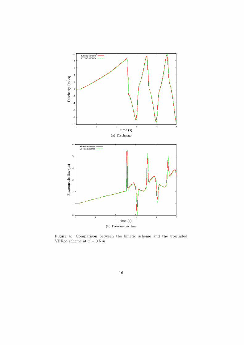
This numerical test intend to reproduce a “sharp” water hammer exper-iment inducing large oscillation of the piezometric level and the discharge asshowed in Fig. 4. From a numerical point of view, it is a “hard” numericaltest.

In order to validate numerically this approach and due to the lack ofexperimental data in the case of variable cross section pipe, we comparethe result of the presented numerical scheme with those obtained by theupwinded VFRoe scheme [2]. Results are represented on Fig. 4 wherewe plot the piezometric line and the discharge for both schemes at pointx = 0.5 m.

Altough the obtained results show small differences, the behavior ofeach solutions are in a good agreement and particularly with respect to thelocalisation of points where the pressure should be potentially dangerous(reaching large values) for instance, for hydroelectric installation. Thisshort and “sharp” water hammer test allows us to validate numerically thekinetic scheme in presence of non-conservative terms.

12

Numerical validation of the upwinding of the friction.In this second example, in order to validate numerically the discretisa-

tion of terms which are neither conservative nor non-conservative, moreprecisely for the friction term, we consider a pipe with uniform section and0-slope to focus only on this term.

We compare the presented numerical scheme to the kinetic schemewhere the friction term is approximated by the cell-centered one. It simplymeans that we use the variable W = (Z, S, cos θ) instead of (11) and weadd the cell-centered approximation of the friction (0,Kn

i uni |un

i |)t to theright hand side of Equation (15)). This comparison is made for severalvalue of the Manning-Strickler coefficient.

To this end, the numerical experiment is performed on a 100 m longclosed pipe with constant section of diameter 2 m. The simulation startsfrom a “double dam break”, as displayed on Fig. 3. The upstream anddownstream condition are identical: the piezometric head increases linearlyfrom 1.8 to 2.1 meters in 30 s (see Fig. 3).Others parameters are:

Discretisation points : 100,Delta x (m) : 1,CFL : 0.8,Simulation time : 100.Sound speed : 20.

where the Manning-Strickler coefficient is taken successively

1

Ks= 0.001, 0.02 and 0.1.

0

0.5

1

1.5

2

0 20 40 60 80 100

Piez

omet

ric

line

(m)

x (m)

(a) Initial state

0

0.5

1

1.5

2

0 20 40 60 80 100

Piez

omet

ric

leve

l (m

)

Times (s)

Prescribed upstream and downstream boundary conditionUpper part of the pipe

(b) Prescribed boundary conditions

Figure 3: Initial state and boundary conditions

13

The results are displayed on Fig. 5– Fig. 7. They represent the measure-ment reading of the piezometric level and the discharge at point x = 18.5 m.As well as Fig. 5 (for 1/Ks = 0.001) and Fig. 6 for 1/Ks = 0.02, i.e. forsmall friction, the results are in a good agreement while some small differ-ences (represented by a shift on the piezometric level and the discharge)are observed in the case of high friction (i.e. 1/Ks = 0.1). However, as wecan see on Fig. 8, the difference decreases when ∆x decreases. Thus, thisseries of tests allows to numerically validate the proposed upwinding of thesource terms.

5 Conclusion

We have presented a global manner to upwind conservative and non-conservativesource terms. To this end, we have used the definition of the non-conservativeproduct of [3] which allows to recover the classical upwinding of conserva-tive terms.

Using the notion of dynamic slope, we have also proposed an upwindingfor a source term which is neither conservative nor non-conservative in aFVK framework. In this paper, we have deal with the friction given by theManning-Strickler law. This approach has been numerically validated.

Finally, the combination of all these quantities into a single one is anelegant and easy way to construct a kinetic scheme with reflections bydescribing the potential barrier as function of the source terms.

Acknowledgements

The authors wish to thank the referee for its careful reading of the previousversion of the manuscript and useful remarks.The second author was supported by the ERC Advanced Grant FP7-246775NUMERIWAVES.

References

[1] C. Bourdarias, M. Ersoy, and S. Gerbi. A kinetic scheme for pressurizedflows in non uniform closed water pipes. Monografias de la Real Academia

de Ciencias de Zaragoza, 31:1–20, 2009.

[2] C. Bourdarias, M. Ersoy, and S. Gerbi. A model for unsteady mixed flowsin non uniform closed water pipes and a well-balanced finite volume scheme.International Journal On Finite Volumes, 6(2):1–47, 2009.

[3] G. Dal Maso, P. G. Lefloch, and F. Murat. Definition and weak stability ofnonconservative products. J. Math. Pures Appl., 74(6):483–548, 1995.

14

[4] M. Ersoy Modelisation, analyse mathematique et numerique de diversecoulements compressibles ou incompressibles en couche mince. PhD Thesis,Chambery, France, 2010.

[5] J.M. Greenberg and A.Y. LeRoux. A well balanced scheme for the numericalprocessing of source terms in hyperbolic equation. SIAM J. Numer. Anal.,33(1):1–16, 1996.

[6] B. Perthame and C. Simeoni. A kinetic scheme for the Saint-Venant systemwith a source term. Calcolo, 38(4):201–231, 2001.

15

-10

-8

-6

-4

-2

0

2

4

6

8

10

0 1 2 3 4 5

Dis

char

ge (

m3 /s

)

time (s)

Kinetic schemeVFRoe scheme

(a) Discharge

0

1

2

3

4

5

6

0 1 2 3 4 5

Piez

omet

ric

line

(m)

time (s)

Kinetic schemeVFRoe scheme

(b) Piezometric line

Figure 4: Comparison between the kinetic scheme and the upwindedVFRoe scheme at x = 0.5m.

16

-8

-6

-4

-2

0

2

4

6

8

0 20 40 60 80 100

Dis

char

ge (

m3 /s

)

Times (s)

Cell-centered approximation of the frictionUpwinded approximation of the friction

(a) Discharge at x = 18.5 m

-4

-2

0

2

4

6

8

0 20 40 60 80 100

Piez

omet

ric

leve

l (m

)

Times (s)


Upper and lower part of the pipe

(b) Piezometric level at x = 18.5 m

Figure 5: Comparison for 1/Ks = 0.001.

17

-6

-4

-2

0

2

4

6

8

0 20 40 60 80 100

Dis

char

ge (

m3 /s

)

Times (s)



-4

-2

0

2

4

6

8

0 20 40 60 80 100

Piez

omet

ric

leve

l (m

)

Times (s)





18

-1.5

-1

-0.5

0

0.5

1

1.5

2

2.5

3

0 20 40 60 80 100

Dis

char

ge (

m3 /s

)

Times (s)



-4

-2

0

2

4

6

8

0 20 40 60 80 100

Piez

omet

ric

leve

l (m

)

Times (s)





19

-1.5

-1

-0.5

0

0.5

1

1.5

2

2.5

3

0 20 40 60 80 100

Dis

char

ge (

m3 /s

)

Times (s)



-4

-2

0

2

4

6

8

0 20 40 60 80 100

Piez

omet

ric

leve

l (m

)

Times (s)




Figure 8: Comparison for 1/Ks = 0.1 with ∆x = 0.5.

20

Documents

A kinetic scheme for transient mixed ﬂows in non uniform