A Kernel Two-Sample Test for Functional Data

George Wynne1 and Andrew B. Duncan1,2

1Imperial College London, Department of Mathematics2The Alan Turing Institute

Abstract

We propose a nonparametric two-sample test procedure based on Maximum MeanDiscrepancy (MMD) for testing the hypothesis that two samples of functions have thesame underlying distribution, using kernels defined on function spaces. This construc-tion is motivated by a scaling analysis of the efficiency of MMD-based tests for datasetsof increasing dimension. Theoretical properties of kernels on function spaces and theirassociated MMD are established and employed to ascertain the efficacy of the newlyproposed test, as well as to assess the effects of using functional reconstructions basedon discretised function samples. The theoretical results are demonstrated over a rangeof synthetic and real world datasets.

1 IntroductionNonparametric two-sample tests for equality of distributions are widely studied instatistics, driven by applications in goodness-of-fit tests, anomaly and change-pointdetection and clustering. Classical examples of such tests include the Kolmogorov-Smirnov test [41, 69, 62] and Wald-Wolfowitz runs test [84] with subsequent multi-variate extensions [25].

Due to advances in the ability to collect large amounts of real time or spatiallydistributed data there is a need to develop statistical methods appropriate for functionaldata, where each data sample is a discretised function. Such data has been studied fordecades in the Functional Data Analysis (FDA) literature [32, 35] particularly in thecontext of analysing populations of time series, or in statistical shape analysis [45].More recently, due to this modern abundance of functional data, increased study hasbeen made in the machine learning literature for algorithms suited to such data [7, 15,37, 12, 88].

In this paper we consider the case where the two probability distributions beingcompared are supported over a real, separable Hilbert space, for example L2(D) withD ⊂ Rd and we have discretised observations of the function samples. If the samplesconsist of evaluations of the functions over a common mesh of points, then well-known

1

arX

iv:2

008.

1109

5v2

[m

ath.

ST]

19

Oct

202

0

methods for nonparametric two-sample testing for vector data can be used directly.Aside from the practical issue that observations are often made on irregular meshes foreach different sample there is also the issue of degrading performance of classical testsas mesh size increases, meaning the observed vectors are high dimensional. As is typi-cal with nonparametric two-sample tests, the testing power will degenerate rapidly withincreasing data dimension. We therefore seek to better understand how to develop test-ing methods which are not strongly affected by the mesh resolution, exploiting intrinsicstatistical properties of the underlying functional probability distributions.

In the past two decades kernels have seen a surge of use in statistical applications[47, 28, 78, 9]. In particular, kernel based two-sample testing [28, 27] has becomeincreasingly popular. These approaches are based on a distance on the space of proba-bility measures known as Maximum Mean Discrepancy. Given two probability dis-tributions P and Q, a kernel k is employed to construct a mapping known as themean embedding, of the two distributions into an infinite dimensional ReproducingKernel Hilbert Space (RKHS). The MMD between P and Q, denoted MMDk(P,Q) isgiven by the RKHS norm of the difference between the two embeddings, and definesa pseudo-metric on the space of probability measures. This becomes a metric if k ischaracteristic, see Section 3. By the kernel trick, MMD simplifies to a closed form,up to expectations, with respect to P and Q, which can be estimated unbiasedly usingMonte Carlo simulations.

A major advantage of kernel two-sample tests is that they can be constructed on anyinput space which admits a well-defined kernel, including Riemannian manifolds [55],as well as discrete structures such as graphs [66] and strings [26]. The flexibility in thechoice of kernel is one of the strengths of MMD-based testing, where a priori knowl-edge of the structure of the underlying distributions can be encoded within the kernel toimprove the sensitivity or specificity of the corresponding test. The particular choice ofkernel strongly influences the efficiency of the test, however a general recipe for con-structing a good kernel is still an open problem. On Euclidean spaces, radial basis func-tion (RBF) kernels are often used, i.e. kernels of the form k(x, y) = φ(γ−1‖x− y‖2),where ‖·‖2 is the Euclidean norm, φ : R+ → R+ is a function and γ > 0 is the band-width. Numerous kernels used in practice belong to this class of kernels, including theGaussian kernel φ(r) = e−r

2/2, the Laplace kernel φ(r) = e−r and others includ-ing the rational quadratic kernel, the Matern kernel and the multiquadric kernel. Theproblem of selecting the bandwidth parameter to maximise test efficiency over a partic-ular input space has been widely studied. One commonly used strategy is the medianheuristic where the bandwidth is chosen to be the median of the inter-sample distance.Despite its popularity, there is only limited understanding of the median heuristic, withsome notable exceptions. In Ramdas et al. [58, 59] the authors investigate the dimin-ishing power of the kernel two-sample test using a Gauss kernel for distributions ofwhite Gaussian random vectors with increasing dimension, demonstrating that underappropriate alternatives, the power of the test will decay with a rate dependent on therelative scaling of γ with respect to dimension. Related to kernel based tests are energydistance tests [79, 80], the relationship was made clear in Sejdinovic et al. [64].

There has been relatively little work on understanding the theoretical properties ofkernels on function spaces. A Gauss type kernel on L2([0, 1]) was briefly considered in

2

Christmann and Steinwart [16, Example 3]. Recently, in Chevyrev and Oberhauser [15]a kernel was defined on the Banach space of paths on [0, 1] of unbounded 1-variation,using a novel approach based on path signatures, demonstrating that this is a charac-teristic kernel over the space of such paths. The associated MMD has been employedas a loss function to train models generating stochastic processes [40]. Furthermore, inNelsen and Stuart [50] the authors propose an extension of the random Fourier featurekernel of Rahimi and Recht [57] to the setting of an infinite dimensional Banach space,with the objective of regression between Banach spaces. This paper will build on as-pects of these works, but with a specific emphasis on two-sample testing for functionaldata.

Two-sample testing in function spaces has received much attention in FDA and isstudied in a variety of contexts. Broadly speaking there are two classes of methods.The first approach seeks to initially reduce the problem to a finite dimensional problemthrough a projection onto a finite orthonormal basis within the function space, typicallyusing principal components, and then makes use of standard multivariate two-sampletests [4, 43]. The second approach poses a two-sample test directly on function space[2, 10, 34, 56, 11]. Many of these works construct the test on the Hilbert space L2(D)using the L2(D) norm as the testing statistic. A priori, it is not obvious why this normwill be well suited to the testing problem, in general. Investigation into the impact ofthe choice of distance in distanced based tests for functional data has been studied inthe literature [14, 13, 90] and a distance other than L2(D) for the functional data wasadvocated. This motivates the investigation into kernels which involve distances otherthan L2(D) in their formulation. In many works, the two-sample tests are designed tohandle a specific class of discrepancy, such as a shift in mean, such as Horvath et al.[33] and Zhang et al. [89], or a shift in covariance structure [52, 23, 24].

This paper has two main aims. First, to naturally generalise the finite dimensionaltheory of kernels to real, separable Hilbert spaces to establish kernels that are char-acteristic, identify their RKHS and establish topological properties of the associatedMMD. In particular the proof of characterticness builds upon the spectral methods in-troduced in Sriperumbudur et al. [72] and the weak convergence results build uponSimon-Gabriel and Scholkopf [67]. Second, we apply such kernels to the two-sampletesting problem and analyse the power of the tests as well as the statistical impact ofperforming the tests using data reconstructed from discrete functional observations.

The specific contributions are as follows.

1. For Gaussian processes, we identify a scaling of the Gauss kernel bandwidth withmesh-size which results in testing power which is asymptotically independent ofmesh-size, under mean-shift alternatives. In the scaling of vanishing mesh-sizewe demonstrate that the associated kernel converges to a kernel over functions.

2. Motivated by this, we construct a family of kernels defined on real, separableHilbert spaces and identify sufficient conditions for the kernels to be characteris-tic, when MMD metrises the weak topology and provide an explicit constructionof the reproducing kernel Hilbert space for a Gauss type kernel.

3. Using these kernels we investigate the statistical effect of using reconstructedfunctional data in the two-sample test.

3

4. We numerically validate our theory and compare the kernel based test with estab-lished two-sample tests from the functional data analysis literature.

The remainder of the paper is as follows. Section 2 covers preliminaries of mod-elling random functional data such as the Karhunen-Loeve expansion and Gaussianmeasures. Section 3 recalls some important properties of kernels and their associatedreproducing kernel Hilbert spaces, defines maximum mean discrepancy and the kerneltwo-sample test. Section 4 outlines the scaling of test power that occurs when an in-creasingly finer observation mesh is used for functional data. Section 5 defines a broadclass of kernels and offers an integral feature map interpretation as well as outliningwhen the kernels are characteristic, meaning the two-sample test is valid. Section 6highlights the statistical impact of fitting curves to discretised functions before per-forming the test. A relationship between MMD and weak convergence is highlightedand closed form expressions for the MMD and mean-embeddings when the distribu-tions are Gaussian processes are given. Section 7 provides multiple examples of choicesfor the kernel hyper parameters and principled methods of constructing them. Section8 contains multiple numerical experiments validating the theory in the paper, a simula-tion is performed to validate the scaling arguments of Section 4 and synthetic and realdata sets are used to compare the performance of the kernel based test against existingfunctional two-sample tests. Concluding remarks and thoughts about future work areprovided in Section 9.

2 Hilbert Space Modelling of Functional DataIn this paper we shall follow the Hilbert space approach to functional data analysisand use this section to outline the required preliminaries [17, 35]. Before discussingrandom functions we establish notation for families of operators that will be used ex-tensively. Let X be a real, separable Hilbert space with inner product 〈·, ·〉X then L(X )denotes the set of bounded linear maps from X to itself, L+(X ) denotes the subset ofL(X ) of operators that are self-adjoint (also known as symmetric) and non-negative,meaning 〈Tx, y〉X ≥ 0 ∀x, y ∈ X . The subset of L+(X ) of trace class operators isdenoted L+

1 (X ) and by the spectral theorem [74, Theorem A.5.13] such operators canbe diagonalised. This means for every T ∈ L+

1 (X ) there exists an orthonormal basisof eigenfunctions en∞n=1 in X such that Tx =

∑∞n=1 λn〈x, en〉X en, where λn∞n=1

are non-negative eigenvalues and the trace satisfies Tr(T ) =∑∞

n=1 λn < ∞. Whenthe eigenvalues are square summable the operator is called Hilbert-Schmidt and theHilbert-Schmidt norm is ‖T‖2HS =

∑∞n=1 λ

2n.

We now outline the Karhunen-Loeve expansion of stochastic processes. Let x(·)be a stochastic process in X = L2([0, 1]), note the following will hold for a stochasticprocess taking values in any real, separable Hilbert space but we focus on L2([0, 1])since it is the most common setting for functional data. Suppose that the point-wise covariance function E[x(s)x(t)] = k(s, t) is continuous, then the mean func-tion m(t) = E[X(t)] is also in X . Define the covariance operator Ck : X → Xassociated with X by Cky(t) =

∫ 10 k(s, t)y(s)ds. Then Ck ∈ L+

1 (X ) and de-note the spectral decomposition Cky =

∑∞n=1 λn〈y, en〉X en. The Karhunen-Loeve

4

(KL) expansion [76, Theorem 11.4] provides a characterisation of the law of the pro-cess x(·) in terms of an infinite-series expansion. More specifically, we can writex(·) ∼ m+

∑∞n=1 λ

1/2n ηnen(·), where ηn∞n=1 are unit-variance uncorrelated random

variables. Additionally, Mercer’s theorem [75] provides an expansion of the covarianceas k(s, t) =

∑∞n=1 λnen(s)en(t) where the convergence is uniform.

An important case of random functions are Gaussian processes [60]. Given a kernelk, see Section 3, and a function m we say x is a Gaussian process with mean functionm and covariance function k if for every finite collection of points snNn=1 the ran-dom vector (x(s1), . . . , x(sN )) is a multivariate Gaussian random variable with meanvector (m(s1), . . . ,m(sN )) and covariance matrix k(sn, sm)Nn,m=1. The mean func-tion and covariance function completely determines the Gaussian process. We writex ∼ GP(m, k) to denote the Gaussian process with mean function m and covariancefunction k. If x ∼ GP(0, k) then in the Karhunen-Loeve representation ηn ∼ N (0, 1)and the ηn are all independent.

Gaussian processes that take values in X can be associated with Gaussian measuresonX . Gaussian measures are natural generalisations of Gaussian distributions on Rd toinfinite dimensional spaces, which are defined by a mean element and covariance oper-ator rather than a mean vector and covariance matrix, for an introduction see Da Prato[18, Chapter 1]. Specifically x ∼ GP(m, k) can be associated with the Gaussian mea-sure Nm,Ck with mean m and covariance operator Ck, the covariance operator associ-ated with k as outlined above. Similarly given any m ∈ X and C ∈ L+

1 (X ) then thereexists a Gaussian measureNm,C with meanm and covariance operatorC [18, Theorem1.12]. In fact, the Gaussian measure Nm,C is characterised as the unique probabilitymeasure on X with Fourier transform Nm,C(y) = exp(i〈m, y〉X − 1

2〈Cy, y〉X ). Fi-nally, if C is injective then a Gaussian measure with covariance operator C is callednon-degenerate and has full support on X [18, Proposition 1.25].

3 Reproducing Kernel Hilbert Spaces and Maxi-mum Mean DiscrepancyThis section will outline what a kernel and a reproducing kernel Hilbert space is withexamples and associated references. Subsection 3.1 defines kernels and RKHS, Sub-section 3.2 defines MMD and the corresponding estimators and Subsection 3.3 outlinesthe testing procedure.

3.1 Kernels and Reproducing Kernel Hilbert SpacesGiven a nonempty set X a kernel is a function k : X × X → R which is symmetric,meaning k(x, y) = k(y, x), for all x, y ∈ X , and positive definite, that is, the matrixk(xn, xm); n,m ∈ 1, . . . , N is positive semi-definite, for all xnNn=1 ⊂ X andfor N ∈ N. For each kernel k there is an associated Hilbert space of functions over Xknown as the reproducing kernel Hilbert space (RKHS) denoted Hk(X ) [6, 74, 22].RKHSs have found numerous applications in function approximation and inference fordecades since their original application to spline interpolation [83]. Multiple detailed

5

surveys exist in the literature [61, 54]. The RKHS associated with k satisfies the fol-lowing two properties i). k(·, x) ∈ H(X ) for all x ∈ X ii). 〈f, k(·, x)〉H(X ) = f(x) forall x ∈ X and f ∈ H(X ). The latter is known as the reproducing property. The RKHSis constructed from the kernel in a natural way. The linear span of a kernel k withone input fixedH0(X ) =

∑Nn=1 ank(·, xn) : N ∈ N, anNn=1 ⊂ R, xnNn=1 ⊂ X

is a pre-Hilbert space equipped with the following inner product 〈f, g〉H0(X ) =∑N

n=1

∑Mm=1 anbmk(xn, ym) where f =

∑Nn=1 ank(·, xn) and g =∑M

m=1 bmk(·, ym). The RKHS Hk(X ) of k is then obtained from H0(X ) throughcompletion. More specificallyHk(X ) is the set of functions which are pointwise limitsof Cauchy sequences in H0(X ) [6, Theorem 3]. The relationship between kernels andRKHS is one-to one, for every kernel the RKHS is unique and for every Hilbert spaceof functions such that there exists a function k satisfying the two properties aboveit may be concluded that the k is unique and a kernel. This result is known as theAronszajn theorem [6, Theorem 3].

A kernel k on X ⊆ Rd is said to be translation invariant if it can be written ask(x, y) = φ(x − y) for some φ. Bochner’s theorem, Theorem 10 in the Appendix,tells us that if k is continuous and translation invariant then there exists a Borel meaureon X such that µk(x − y) = k(x, y) and we call µk the spectral measure of k. Thespectral measure is an important tool in the analysis of kernel methods and shall becomeimportant later when discussing the two-sample problem.

3.2 Maximum Mean DiscrepancyGiven a kernel k and associated RKHS Hk(X ) let P be the set of Borel probabilitymeasures on X and assuming k is measurable define Pk ⊂ P as the set of all P ∈ Pksuch that

∫k(x, x)

12dP (x) < ∞. Note that Pk = P if and only if k is bounded [72,

Proposition 2] which is very common in practice and shall be the case for all kernelsconsidered in this paper. For P,Q ∈ Pk we define the Maximum Mean Discrepancydenoted MMDk(P,Q) as follows MMDk(P,Q) = sup‖f‖Hk(X )≤1

∣∣∫ fdP − ∫ fdQ∣∣.This is an integral probability metric [48, 72] and without further assumptions defines apseudo-metric on Pk, which permits the possibility that MMDk(P,Q) = 0 but P 6= Q.

We introduce the mean embedding ΦkP of P ∈ Pk into Hk(X ) defined byΦkP =

∫k(·, x)dP (x). This can be viewed as the mean in Hk(X ) of the function

k(x, ·) with respect to P in the sense of a Bochner integral [35, Section 2.6]. FollowingSriperumbudur et al. [72, Section 2] this allows us to write

MMDk(P,Q)2 =

(sup

‖f‖Hk(X )≤1

∣∣∣∣∫ fdP −∫fdQ

∣∣∣∣)2

=

(sup

‖f‖Hk(X )≤1|〈ΦkP − ΦkQ, f〉|

)2

= ‖ΦkP − ΦkQ‖2Hk(X ). (1)

The crucial observation which motivates the use of MMD as an effective measure ofdiscrepancy is that the supremum can be eliminated using the reproducing property of

6

the inner product [72, Section 2]. This yields the following closed form representation

MMDk(P,Q)2 =

∫ ∫k(x, x′)dP (x)dP (x′) +

∫ ∫k(y, y′)dQ(y)dQ(y′)

− 2

∫ ∫k(x, y)dP (x)dQ(y). (2)

It is clear that MMDk is a metric over Pk if and only if the map Φk : Pk → Hk(X )is injective. Given a subset P ⊆ Pk, a kernel is characteristic to P if the map Φk isinjective over P. In the case that P = P we just say that k is characteristic. Variousworks have provided sufficient conditions for a kernel over finite dimensional spaces tobe characteristic [72, 73, 67].

Given independent samples Xn = xini=1 from P and Ym = yimi=1 from Q wewish to estimate MMDk(P,Q)2. A number of estimators have been proposed. Forclarity of presentation we shall assume that m = n, but stress that all of the followingcan be generalised to situations where the two data-sets are unbalanced. Given samplesXn and Yn, the following U-statistic is an unbiased estimator of MMD2

k(P,Q)2

MMDk(Xn, Yn)2 :=1

n(n− 1)

n∑i 6=j

h(zi, zj), (3)

where zi = (xi, yi) and h(zi, zj) = k(xi, xj) + k(yi, yj)− k(xi, yj)− k(xj , yi). Thisestimator can be evaluated in O(n2) time. An unbiased linear time estimator proposedin Jitkrittum et al. [36] is given by

MMDk,lin(Xn, Yn)2 :=2

n

n/2∑i=1

h(z2i−1, z2i), (4)

where it is assumed that n is even. While the cost for computing MMDk,lin(Xn, Yn)2

is only O(n) this comes at the cost of reduced efficiency, i.e. Var(MMDk(Xn, Yn)2) <

Var(MMDk,lin(Xn, Yn)2), see for example Sutherland [77]. Various probabilisticbounds have been derived on the error between the estimator and MMDk(P,Q)2 [28,Theorem 10, Theorem 15].

3.3 The Kernel Two-Sample TestGiven independent samples Xn = xini=1 from P and Yn = yini=1 from Q we seekto test the hypothesis H0 : P = Q against the alternative hypothesis H1 : P 6= Q with-out making any distributional assumptions. The kernel two-sample test of Gretton et al.[28] employs an estimator of MMD as the test statistic. Indeed, fixing a characteristickernel k, we reject H0 if MMDk(Xn, Yn)2 > cα, where cα is a threshold selected toensure a false-positive rate of α. While we do not have a closed-form expression forcα, it can be estimated using a permutation bootstrap. More specifically, we randomlyshuffle Xn ∪ Yn, split it into two data sets X ′n and Y ′n, from which MMDk(X

′n, Y

′n)2

is calculated. This is repeated numerous times so that an estimator of the threshold cα

7

is then obtained as the (1 − α)-th quantile of the resulting empirical distribution. Thesame test procedure may be performed using the linear time MMD estimator as the teststatistic.

The efficiency of a test is characterised by its false-positive rate α and its its false-negative rate β. The power of a test is a measure of its ability to correctly reject the nullhypothesis. More specifically, fixing α, and obtaining an estimator cα of the threshold,we define the power of the test at α to be P(nMMDk(Xn, Yn)2 ≥ cα). Invoking thecentral limit theorem for U-statistics [65] we can quantify the decrease in variance ofthe unbiased MMD estimators, asymptotically as n→∞.

Theorem 1. [28, Corollary 16] Suppose that Ex∼P,y∼Q[h2(x, y)] < ∞. Then un-der the alternative hypothesis P 6= Q, the estimator MMDk(Xn, Yn)2 converges indistribution to a Gaussian as follows

√n(

MMDk(Xn, Yn)2 −MMD2k(P,Q)

)D−→ N (0, 4ξ1), n→∞,

where ξ1 = Varz [Ez′ [h(z, z′)]]. An analogous result holds for the linear-time estima-tor, with ξ2 = Varz,z′ [h(z, z′)] instead of ξ1.

In particular, under the conditions of Theorem 1, for large n, the power of the testwill satisfy the following asymptotic result

P(nMMDk(Xn, Yn)2 > cα

)≈ Φ

(√n

MMDk(P,Q)2

2√ξ1

− cα

2√nξ1

), (5)

where Φ is the CDF for a standard Gaussian distribution and ξ1 = Varz [Ez′ [h(z, z′)]].The analogous result for the linear-time estimator holds with ξ2 = Varz,z′ [h(z, z′)]instead of ξ1 [59, 42]. This suggests that the test power can be maximised by max-imising MMDk(P,Q)2/

√ξ1 which can be seen as a signal-to-noise-ratio [42]. It is

evident from previous works that the properties of the kernel will have a very signifi-cant impact on the power of the test, and methods have been proposed for increasingtest power by optimising the kernel parameters using the signal-to-noise-ratio as anobjective [78, 59, 42].

4 Resolution Independent Tests for Gaussian Pro-cessesTo motivate the construction of kernel two-sample tests for random functions, in thissection we will consider the case where the samplesXn and Yn are independent realisa-tions of two Gaussian processes, observed along a regular mesh ΞN = t1, . . . , tN ofN points in D where D ⊂ Rd is some compact set. Therefore N will be the dimensionof the observed vectors. To develop ideas, we shall focus on a mean-shift alternative,where the underlying Gaussian processes are given by GP(0, k0) and GP(m, k0) re-spectively, where k0 is a covariance function, and m ∈ L2(D) is the mean function.We use the subscript on k0 to distinguish it from the kernel k we use to perform the

8

test. We will use the linear time test due to easier calculations. This reduces to a multi-variate two-sample hypothesis test problem on RN , with samples Xn = xini=1 fromP = N (0,Σ) and Yn = yini=1 from Q = N (mN ,Σ), where Σi,j = k0(ti, tj) fori, j = 1, . . . , N and mN = (m(t1), . . . ,m(tN ))>.

We consider applying a two-sample kernel test as detailed in Section 3, with aGaussian kernel k(x, y) = exp(−1

2γ−2N ‖x− y‖22) on RN where γN may depend on N .

The large N limit was studied in Ramdas et al. [58] but not in the context of functionaldata. This motivates the question whether there is a scaling of γN with respect to Nwhich, employing the structure of the underlying random functions, guarantees thatthe statistical power remains independent of the mesh size N . To better understandthe influence of bandwidth on power, we use the signal-to-noise ratio as a convenientproxy, and study its behaviour in the large N limit. We say the mesh ΞN satisfies theRiemann scaling property if 1

N ‖mN‖22 = 1N

∑Ni=1m(ti)

2 →∫Dm(t)2dt = ‖m‖2L2(D)

as N → ∞ for all m ∈ L2(D), this will be used in the next result to characterise thesignal-to-noise ratio from the previous subsection.

Proposition 1. Let P,Q be as above with ΞN satisfying the Riemann scaling propertyand γN = Ω(Nα) with α > 1/2 then if k0(s, t) = δst

MMDk(P,Q)2

√ξ2

∼√N‖m‖2L2(D)

2√

1 + ‖m‖2L2(D)

, (6)

and if k0 is continuous and bounded then

MMDk(P,Q)2

√ξ2

∼‖m‖2L2(D)

2√‖Ck0‖2HS + ‖C1/2

k0m‖2

L2(D)

, (7)

where ∼ means asymptotically equal in the sense that the ratio of the left and righthand side converges to one as N →∞.

The proof of this result is in the Appendix and generalises Ramdas et al. [58] byconsidering non-identity Σ. The way this ratio increases with N , the number of obser-vation points, in the white noise case makes sense since each observation is revealingnew information about the signal as the noise is independent at each observation. Onthe other hand the non-identity covariance matrix means the noise is not independentat each observation and thus new information is not obtained at each observation point.Indeed the stronger the correlations, meaning the slower the decay of the eigenvaluesof the covariance operator Ck0 , the smaller this ratio shall be since the Hilbert-Schmidtnorm in the denominator will be larger.

It is important to note that the ratio in the right hand sides of (7) and (6) are in-dependent of the choice of α once α > 1/2 meaning that once greater than 1/2 thisparameter will be ineffective for obtaining greater testing power. The next subsectiondiscusses how α = 1/2 provides a scaling resulting in kernels defined directly overfunction spaces, facilitating other methods to gain better test power.

9

4.1 Kernel ScalingProposition 1 does not include the case γN = Θ(N1/2) however it can be shown thatthe ratio does not degenerate in this case, see Theorem 7 and Theorem 8. In fact, thetwo different scales of the ratio, when Σ is the identity matrix or a kernel matrix, stilloccur. This is numerically verified in Section 8.

Suppose γN = γ0N1/2 for some γ0 ∈ R and one uses a kernel of the form

k(x, y) = f(γ−2N ‖x − y‖22) over RN for some continuous f . Suppose now though

that our inputs shall be xN , yN , discretisations of functions x, y ∈ L2(D) observed ona mesh ΞN that satisfies the Riemann scaling property. Then as the mesh gets finer weobserve the following scaling

k(xN , yN ) = f(γ−2N ‖xN − yN‖22)

N→∞−−−−→ f(γ−20 ‖x− y‖2L2(D)).

Therefore the kernel, as the discretisation resolution increases, will converge to a kernelover L2(D) where the Euclidean norm is replaced with the L2(D) norm. For examplethe Gauss kernel would become exp(−γ−2

0 ‖x− y‖2L2(D)).This scaling coincidentally is similar to the scaling of the widely used median

heuristic defined as

γ2 = Median‖a− b‖22 : a, b ∈ xini=1 ∪ yimi=1, a 6= b

, (8)

where xini=1 are the samples from P , yini=1 samples from Q. It was not designedwith scaling in mind however in Ramdas et al. [59] it was noted that it results in aγ2 = Θ(N) scaling for the mean shift, identity matrix case. The next lemma makesthis more precise by relating the median of the squared distance to its expectation.

Lemma 1. Let P = N (µ1,Σ1) and Q = N (µ2,Σ2) be independent Gaussian distri-butions on RN then Ex∼P,y∼Q[‖x− y‖22] = Tr(Σ1 + Σ2) + ‖µ1 − µ2‖22 and∣∣∣∣Medianx∼P,y∼Q[‖x− y‖22]

Ex∼P,y∼Q[‖x− y‖22]− 1

∣∣∣∣ ≤ √2

(1− ‖µ1 − µ2‖42

(Tr(Σ1 + Σ2) + ‖µ1 − µ2‖22)2

) 12

,

in particular if P,Q are discretisations of Gaussian processesGP(m1, k1),GP(m2, k2) on a mesh ΞN of N points satisfying the Riemannscaling property over some compact D ⊂ Rd with m1,m2 ∈ L2(D) and k1, k2

continuous then Ex∼P,y∼Q[‖x − y‖22] ∼ N(Tr(Ck1 + Ck2) + ‖m1 −m2‖2L2(D)) andas N →∞ the right hand side of the above inequality converges to

√2

(1−

‖m1 −m2‖4L2(D)

(Tr(Ck1 + Ck2) + ‖m1 −m2‖2L2(D))2

) 12

.

The above lemma does not show that the median heuristic results in γN = γ0N1/2

but relates it to the expected squared distance which does scale directly as γ0N1/2.

Therefore investigating the properties of such a scaling is natural.Since L2(D) is a real, separable Hilbert space when using kernels defined directly

over L2(D) in later sections we can leverage the theory of probability measures on such

10

Hilbert spaces to deduce results about the testing performance of such kernels. In fact,we shall move past L2(D) and obtain results for kernels over arbitrary real, separableHilbert spaces. Note that a different scaling of γN would not result in such a scaling ofthe norm to L2(D) so such theory cannot be applied.

5 Kernels and RKHS on Function SpacesFor the rest of the paper, unless specified otherwise, for example in Theorem 4, thespaces X ,Y will be real, separable Hilbert spaces with inner products and norms〈·, ·〉X , 〈·, ·〉Y , ‖·‖X , ‖·‖Y . We adopt the notation in Section 2 for various families ofoperators.

5.1 The Squared-Exponential T kernelMotivated by the scaling discussions in Section 4 we define a kernel that acts directlyon a Hilbert space.

Definition 1. For T : X → Y the squared-exponential T kernel (SE-T ) is defined as

kT (x, y) = e−12‖T (x)−T (y)‖2Y .

We use the name squared-exponential instead of Gauss because the SE-T kernel isnot always the Fourier transform of a Gaussian distribution whereas the Gauss kernelon Rd is, which is a key distinction and is relevant for our proofs. Lemma 2 in theAppendix assures us this function is a kernel. This definition allows us to adapt resultsabout the Gauss kernel on Rd to the SE-T kernel since it is the natural infinite dimen-sional generalisation. For example the following theorem characterises the RKHS ofthe SE-T kernel for a certain choice of T , as was done in the finite dimensional casein Minh [46]. Before we state the result we introduce the infinite dimensional gener-alisation of a multi-index, define Γ to be the set of summable sequences indexed byN taking values in N ∪ 0 and for γ ∈ Γ set |γ| =

∑∞n=1 γn, so γ ∈ Γ if and

only if γn = 0 for all but finitely many n ∈ N meaning Γ is a countable set. We setΓn = γ ∈ Γ: |γ| = n and the notation

∑|γ|≥0 shall mean

∑∞n=0

∑γ∈Γn

which is acountable sum.

Theorem 2. Let T ∈ L+(X ) be of the form Tx =∑∞

n=1 λ1/2n 〈x, en〉X en with con-

vergence in X for some orthonormal basis en∞n=1 and bounded positive coefficientsλn∞n=1 then the RKHS of the SE-T kernel is

HkT (X ) =

F (x) = e−12‖Tx‖2X

∑|γ|≥0

wγxγ :

∑|γ|≥0

γ!

λγw2γ <∞

,

where xγ =∏∞n=1 x

γnn , xn = 〈x, en〉X , λγ =

∏∞n=1 λ

γnn and γ! =

∏∞n=1 γn! and

HkT (X ) is equipped with the inner product 〈F,G〉HkT (X ) =∑|γ|≥0

γ!λγwγvγ where

F (x) = e−12‖Tx‖2X

∑|γ|≥0wγx

γ , G(x) = e−12‖Tx‖2X

∑|γ|≥0 vγx

γ .

11

Remark 1. In the proof of Theorem 2 an orthonormal basis ofHkT (X ) is given whichresembles the infinite dimensional Hermite polynomials which are used throughoutinfinite dimensional analysis and probability theory, for example see Da Prato andZabczyk [19, Chapter 10] and Nourdin and Peccati [51, Chapter 2]. In particular theyare used to define Sobolev spaces for functions over a real, separable Hilbert space[19, Theorem 9.2.12] which raises the interesting and, as far as we are aware, openquestion of howHkT (X ) relates to such Sobolev spaces for different choices of T .

For the two-sample test to be valid we need the kernel to be characteristic meaningthe mean-embedding is injective over P , so the test can tell the difference between anytwo probability measures. To understand the problem better we again leverage resultsregarding the Gauss kernel on Rd, in particular the proof in Sriperumbudur et al. [72,Theorem 9] that the Gauss kernel on Rd is characteristic. This uses the fact that theGauss kernel on Rd is the Fourier transform of a Gaussian distribution on Rd whosefull support implies the kernel is characteristic. By choosing T such that the SE-Tkernel is the Fourier transform of a Gaussian measure on X that has full support wecan use the same argument.

Theorem 3. Let T ∈ L+1 (X ) then the SE-T kernel is characteristic if and only if T is

injective.

This is dissatisfyingly limiting since T ∈ L+1 (X ) is a restrictive assumption, for

example it does not include T = I the identity operator. We shall employ a limitargument to reduce the requirements on T . To this end we define admissible maps.

Definition 2. A map T : X → Y is called admissible if it is Borel measurable, contin-uous and injective.

The next result provides a broad family of kernels which are characteristic. It ap-plies for X being more general than a real, separable Hilbert space. A Polish space is aseparable, completely metrizable topological space. Multiple examples of admissibleT are given in Section 7 and are examined numerically in Section 8.

Theorem 4. Let X be a Polish space, Y a real, separable Hilbert space and T anadmissible map then the SE-T kernel is characteristic.

Theorem 4 generalises Theorem 3. A critical result used in the proof is the Minlos-Sazanov theorem, detailed as Theorem 11 in the Appendix, which is an infinite dimen-sional version of Bochner’s theorem. The result allows us to identify spectral propertiesof the SE-T kernel which are used to deduce characteristicness.

5.2 Integral Kernel FormulationLet k0 : R × R → R be a kernel, C ∈ L+

1 (X ) and NC the corresponding mean zeroGaussian measure on X and define kC,k0 : X × X → R as follows

kC,k0(x, y) :=

∫Xk0 (〈x, h〉X , 〈y, h〉X ) dNC(h).

12

Consider the particular case where k0(s, t) = 〈Φ(s),Φ(t)〉F , where Φ : R → F is acontinuous feature map, mapping into a Hilbert space (F , 〈·, ·〉F ), which will typicallybe RF for some F ∈ N. In this case the functions x → Φ(〈x, h〉X ) can be viewedas F–valued random features for each h ∈ X randomly sampled from NC , and kC,k0is very similar to the random feature kernels considered in Nelsen and Stuart [50] andBach [3]. Following these previous works, we may completely characterise the RKHSof this kernel, the result involves L2

NC(X ;F) which is the space of equivalence classes

of functions from X to F that are square integrable in the F norm with respect to NC

and L2(X ) := L2(X ;F).

Proposition 2. Suppose that ψ(x, h) = Φ(〈x, h〉X ) satisfies ψ ∈ L2NC×NC (X ×X ;F)

then the RKHS defined by the kernel kC,k0 is given by

HkC,k0 (X ) =

∫〈v(h), ψ(·, h)〉FdNC(h) : v ∈ L2

NC(X ;F)

⊂ L2

NC(X ).

The proof of this result is an immediate generalization of the real-valued case givenin Nelsen and Stuart [50]. Using the spectral representation of translation invariantkernels we can provide conditions for kC,k0 to be a characteristic kernel.

Proposition 3. If k0 is a kernel over R × R then kC,k0 is a kernel over X × X . If Cis injective and k0 is also continuous and translation invariant with spectral measureµ such that there exists an interval (a, b) ⊂ R with µ(U) > 0 for every open subsetU ⊂ (a, b) then kC,k0 is characteristic.

For certain choices of T the SE-T kernel falls into a family of integral kernels.Indeed, if k0(x, y) = cos(x− y) then kC,k0 is the SE-C

12 kernel

kC,k0(x, y) = NC(x− y) = e−12‖x−y‖2C = e−

12

∑∞n=1 λn(xn−yn)2 ,

where ‖x− y‖2C = 〈C(x− y), x− y〉X , λn∞n=1 are the eigenvalues of C and xn =〈x, en〉 are the coefficients with respect to the eigenfunction basis en∞n=1 of C.

Secondly, let γ > 0 and assume C is non-degenerate and set k0 to be the complexexponential of γ multiplied the by white noise mapping associated withC, see Da Prato[18, Section 1.2.4], then kC,k0 is the SE-γI kernel

kC,k0(x, y) = kγI(x, y) = e−γ2‖x−y‖2X , (9)

Note that kγI is not the Fourier transform of any Gaussian measure on X [44, Proposi-tion 1.2.11] which shows how the integral kernel framework is more general than onlyusing the Fourier transform of Gaussian measures to obtain kernels, as was done inTheorem 3.

The integral framework can yield non-SE type kernels. Let N1 be the measureassociated with the Gaussian distribution N (0, 1) on R, C be non-degenerate andk0(x, y) = N1(x− y) then we have

kC,k0(x, y) =

∫X

∫Reiz〈h,x−y〉dN1(z)dNC(h) =

(‖x− y‖2C + 1

)− 12 . (10)

13

Definition 3. For T : X → Y the inverse multi-quadric T kernel (IMQ-T ) is definedas kT (x, y) =

(‖T (x)− T (y)‖2Y + 1

)−1/2.

By using Proposition 3 we immediately obtain that if T ∈ L+1 (X ) and T is non-

degenerate then the IMQ-T kernel is characteristic. But by the same limiting argumentas Theorem 4 and the integral kernel formulation of IMQ-T we obtain a more generalresult.

Corollary 1. Under the same conditions as Theorem 4 the IMQ-T kernel is character-istic.

6 MMD on Function SpacesIn Section 5 we derived kernels directly over function spaces that were characteristic,meaning that the MMD induced by them is a metric on P(X ). Therefore a two-sampletest based on such kernels may be constructed, as detailed in Section 3, using the sameform of U-statistic estimators and bootstrap technique as the finite dimensional sce-nario. This section will explore properties of the test. Subsection 6.1 will investigatethe effect of performing the test on reconstructions of the random function based onobserved data. Subsection 6.2 will provide explicit calculations for MMD when P,Qare Gaussian processes. Subsection 6.3 discusses the topology on P(X ) induced byMMD and how it relates to the weak topology.

6.1 Influence of Function Reconstruction on MMD Estima-torIn practice, rather than having access to the full realisation of random functions the dataavailable will be some finite-dimensional representation of the functions, for examplethrough discretisation over a mesh, or as a projection onto a finite dimensional basis ofX . Therefore to compute the kernel a user may need to approximate the true underly-ing functions from this finite dimensional representation. We wish to ensure that theeffectiveness of the tests using reconstructed data.

We formalise the notion of discretisation and reconstruction as follows. Assumethat we observe Ixini=1 where xni=1 are the random samples from P and I : X →RN is a discretisation map. For example, I could be point evaluation at some somefixed t1, t2, . . . , tN ∈ D i.e. Ixi = (xi(t1), . . . , xi(tN ))>. Noisy point evaluation canalso be considered in this framework. Then a reconstruction map R : RN → X isemployed so that RIXn = RIxini=1 is used to perform the test, analogously forRIYn. For example, R could be a kernel smoother or a spline interpolation operator.In practice one might have a different number of observations for each function, thefollowing results can be adapted to this case straightforwardly.

Proposition 4. Assume k is a kernel on X satisfying |k(x, y) − k(u, v)| ≤ L‖x −y − (u − v)‖X for all u, v, x, y ∈ X for some L > 0 and let P,Q ∈ P with Xn =

14

xini=1, Yn = yini=1 i.i.d. samples from P,Q respectively with reconstructed dataRIXn = RIxini=1,RIYn = RIyini=1 then∣∣∣∣MMDk(Xn, Yn)2 − MMDk(RIXn,RIYn)2

∣∣∣∣≤ 4L

n

n∑i=1

‖RIxi − xi‖X + ‖RIyi − yi‖X .

Corollary 2. If kT is the SE-T or IMQ-T kernel then the above bound holds with‖T (RIxi)−T (xi)‖Y , ‖T (RIyi)−T (yi)‖Y instead of ‖RIxi−xi‖X , ‖RIyi−yi‖Xwith L = 1√

eand L = 2

3√

3respectively.

An analogous result can be derived for the linear time estimator with the sameproof technique. While Proposition 4 provides a statement on the approximationof MMDk(RIXn,RIYn)2 we are primarily concerned with its statistical properties.Asymptotically, the test efficiency is characterised via the Gaussian approximation inTheorem 1, specifically through the asymptotic variance in (5). The following resultprovides conditions under which a similar central limit theorem holds for the estimatorbased on reconstructed data, with the same asymptotic variance. It imposes conditionson the number of discretisation points per function sample N , the error of the approxi-mations and the number of function samples n.

Theorem 5. Let k satisfy the condition in Proposition 4 and let Xn = xini=1 andYn = yini=1 be i.i.d. samples from P and Q respectively with P 6= Q, and asso-ciated reconstructions RIXn and RIYn based on N(n) dimensional discretisationsIXn and IYn where N(n) → ∞ as n → ∞. If n

12Ex∼P [‖x − RIx‖X ] → 0 and

n12Ey∼P [‖y −RIy‖X ]→ 0 as n→∞, then for ξ = 4Varz [Ez′ [h(z, z′)]]

n12(MMDkT (RIXn,RIYn)2 −MMDkT (P,Q)2

) d−→ N (0, ξ).

A similar result can be derived for the linear time estimator by using the linear timeestimator version of Proposition 4. The discretisation map, number of discretisationsper function sample and the reconstruction map need to combine to satisfy the con-vergence assumption. For example if a weaker reconstruction map is used then moreobservations per function sample will be needed to compensate for this. Additionallyif the discretisation map offers less information about the underlying function, for ex-ample it provides observations that are noise corrupted, then more observations perfunction sample are needed.

We now discuss three settings in which these assumptions hold, relevant to differentapplications. We shall assume that k satisfies the conditions of Proposition 4 and thatT = I .

6.1.1 Linear interpolation of regularly sampled data

Let X = L2([0, 1]) and ΞN(n) = tiN(n)i=1 be a mesh of evaluation points where

ti+1− ti = N(n)−1 for all i and define Ix = (x(t1), . . . , x(tN(n)))> ∈ RN(n). LetR

15

be the piecewise linear interpolant defined as

(RIx)(t) = (x(ti+1)− x(tk))t− titi+1 − ti

+ x(ti), for t ∈ [ti, ti+1).

Suppose that realisations x ∼ P and y ∼ Q are almost surely in C2([0, 1]) and inparticular satisfy Ex∼P [‖x′′‖2X ] <∞ and Ey∼Q[‖y′′‖2X ] <∞. Then

Ex∼P [‖x−RIx‖X ] ≤ 1

N(n)2Ex∼P [‖x′′‖X ],

and analogously for y ∼ Q. Therefore ifN(n) ∼ nα with α > 1/4 then the conditionsof Theorem 5 are satisfied.

6.1.2 Kernel interpolant of quasi-uniformly sampled data

Let X = L2(D) withD ⊂ Rd compact. As in the previous example, I will be the eval-uation operator over a set of points ΞN(n) = tiN(n)

i=1 but now we assume the pointsare placed quasi-uniformly in the scattered data approximation sense, for example reg-ularly placed grid points, see Wynne et al. [87] and Wendland [85, Chapter 4] for othermethod to obtain quasi-uniform points.

We setR as the kernel interpolant using a kernel k0 with RKHS norm equivalent toW ν

2 (D) with ν > d/2, this is achieved by the common Matern and Wendland kernels[85, 38]. For this choice of recovery operator, (RIx)(t) = k0(t,Ξ)K−1

0 I(x) wherek0(t,Ξ) = (k0(t, t1), . . . , k0(t, tN(n)) and K0 is the kernel matrix of k0 over ΞN(n).

Suppose the realisations of P andQ lie almost surely inW τ2 (D) for some τ > d/2,

this assumption is discussed when P,Q are Gaussian processes in Kanagawa et al. [38,Section 4], then

Ex∼P [‖x−RIx‖X ] ≤ CN(n)−(τ∧ν)/d,

for some constant C > 0, with an identical result holding for realisations ofQ [87, 49].It follows that choosing N(n) ∼ n guarantees that the conditions of Theorem 5 hold inthis setting. Here we see that to maintain a scaling of N(n) independent of dimensiond we need the signal smoothness ν, τ to increase with d.

Note that the case where I is pointwise evaluation corrupted by noise may betreated in a similar way by using results from Bayesian non-parametrics, for examplevan der Vaart and van Zanten [82, Theorem 5]. In this case R would be the posteriormean of a Gaussian process that is conditioned on I(x).

6.1.3 Projection onto an orthonormal basis

Let X be an arbitrary real, separable Hilbert space and en∞n=1 be an orthonormalbasis. Suppose that I is a projection operator onto the first N(n) elements of thebasis Ix = (〈x, e1〉X , . . . , 〈x, eN(n)〉X )> and R constructs a function from basis co-

efficients R(β1, . . . , βN(n)) =∑N(n)

i=1 βiei meaning RIx =∑N(n)

i=1 〈x, ei〉X ei. Atypical example on L2([0, 1]) would be a Fourier series representation of the sam-ples xini=1 and yini=1 from which the functions can be recovered efficiently via

16

an inverse Fast Fourier Transform. By Parseval’s theorem Ex∼P [‖x − RIx‖2X ] =∑∞i=N(n)+1 |〈x, ei〉X |2 → 0 as N(n) → ∞. For the conditions of Theorem 5 to hold,

we require that n1/2Ex∼P[∑∞

i=N(n)+1 |〈x, ei〉X |2]→ 0 as n → ∞ which means

N(n) will need to grow in a way to compensate for the auto-correlation of realisationsof P and Q.

In this setting the use of the integral kernels described in Section 5.2 are particularlyconvenient. Indeed, let C =

∑∞i=1 λiei ⊗ ei ∈ L1

+(X ) and consider the integral kernelkC,k0 where k0(s, t) = Φ(s)Φ(t) for a feature map Φ taking values in R. An evaluationof the kernel k(x, y) can then be approximated using a random Fourier feature approach[57] by

k(x, y) ≈ 1

nS

nS∑l=1

Φ

N(n)∑i=1

λ12i xiη

li

Φ

N(n)∑j=1

λ12j yjη

lj

,

where xi = 〈x, ei〉X , yi = 〈y, ei〉X and ηli ∼ N (0, 1) i.i.d. for i = 1, . . . N(n) and l =1, . . . , nS for some nS ∈ N. The permits opportunities to reduce the computational costof MMD tests as judicious choices of Φ will permit accurate approximations of k(x, y)using nS small. Similarly, the weights, λi can be chosen to reduce the dimensionalityof the functions xi and yi.

6.2 Explicit Calculations for Gaussian ProcessesA key property of the SE-T kernel is that the mean-embedding ΦkTP andMMDkT (P,Q)2 have closed form solutions when P,Q are Gaussian measures. Usingthe natural correspondence between Gaussian measures and Gaussian processes fromSection 2 we may get closed form expressions for Gaussian processes. This addressesthe open question regarding the link between Bayesian non-parametrics methods andkernel mean-embeddings that was discussed in Muandet et al. [47, Section 6.2].

Before stating the next result we need to introduce the concept of determinant foran operator, for S ∈ L1(X ) define det(I + S) =

∏∞n=1(1 + λn) where λn∞n=1 are

the eigenvalues of S. The equality det((I + S)(I + R)

)= det(I + S) det(I + R)

holds and is frequently used.

Theorem 6. Let kT be the SE-T kernel for some T ∈ L+(X ) and P = Na,S be anon-degenerate Gaussian measure on X then

ΦkT (Na,S)(x) = det(I + TST )−12 e−

12〈(I+TST )−1T (x−a),T (x−a)〉X .

Theorem 7. Let kT be the SE-T kernel for some T ∈ L+(X ) and P = Na,S , Q =Nb,R be non-degenerate Gaussian measures on X then

MMDkT (P,Q)2 = det(I + 2TST )−12 + det(I + 2TRT )−

12

− 2 det((I + TST )(I + (TRT )

12 (I + TST )−1(TRT )

12 ))− 1

2

× e− 12〈(I+T (S+R)T )−1T (a−b),T (a−b)〉X .

17

These results outline the geometry of Gaussian measures with respect to the dis-tance induced by the SE-T kernel. We see that the means only occur in the formulathrough their difference and if both mean elements are zero then the distance is mea-sured purely in terms of the spectrum of the covariance operators.

Corollary 3. Under the Assumptions of Theorem 7 and that T, S,R commute then

MMDkT (P,Q)2 = det(I + 2TST )−12 + det(I + 2TRT )−

12

− 2 det(I + T (S +R)T )−12 e−

12〈(I+T (S+R)T )−1T (a−b),T (a−b)〉X .

Since the variance terms ξ1, ξ2 from Section 3 are simply multiple integrals of theSE-T kernel against Gaussian measures we may obtain closed forms for them too.Theorem 8 is a particular instance of the more general Theorem 13 in the Appendix.

Theorem 8. Let P = NS , Q = Nm,S be non-degenerate Gaussian measures on X ,T ∈ L+

1 (X ) and assume T and S commute then when using the SE-T kernel

ξ1 = 2 det(ΣS)−12(1 + e−〈(I+3TST )−1Tm,Tm〉X − 2e−

12〈(I+2TST )Σ−1

S Tm,Tm〉X)

− 2 det(I + 2TST )−1(1 + e−〈(I+2TST )−1Tm,Tm〉X − 2e−

12〈(I+2TST )−1Tm,Tm〉X

),

ξ2 = 2 det(I + 4TST )−12(1 + e−〈(I+4TST )−1Tm,Tm〉X

)− 2 det(I + 2TST )−1

(1 + e−〈(I+2TST )−1Tm,Tm〉X − 4e−

12〈(I+2TST )−1Tm,Tm〉X

)− 8 det(ΣS)−

12 e−

12〈(I+2TST )Σ−1

S Tm,Tm〉X ,

where ΣS = (I + TST )(I + 3TST ).

6.3 Weak Convergence and MMDWe know that MMD is a metric on P when k is characteristic, so it is natural to identifythe topology it generates and in particular how it relates to the standard topology forelements of P , the weak topology.

Theorem 9. LetX be a Polish space, k a bounded, continuous, characteristic kernel onX ×X and P ∈ P then Pn

w−→ P implies MMDk(Pn, P )→ 0 and if Pn∞n=1 ⊂ P istight then MMDk(Pn, P )→ 0 implies Pn

w−→ P where w−→ denotes weak convergence.

For a discussion on weak convergence and tightness see Billingsley [8]. The tight-ness is used to compensate for the lack of compactness of X which is often requiredin analogous finite dimensional results. In particular, in Chevyrev and Oberhauser [15]an example where MMDk(Pn, P )→ 0 but Pn but does converge to P was given with-out the assumption of tightness. A precise characterisation of the relationship betweenMMD and weak convergence over a Polish space is an open problem.

7 Practical Considerations for Kernel SelectionWe now present examples and techniques to choose kernels and construct maps T thatare admissible. Two main categories will be discussed, integral operators induced bykernels and situation specific kernels.

18

For the first catergory assume X = Y = L2(D) for some compact D ⊂ Rd and letk0 be a measurable kernel over D × D and set T = Ck0 where Ck0 is the covarianceoperator associated with k0, see Section 2. We call k0 an admissible kernel if Ck0 isadmissible. If k0 is continuous then by Mercer’s theorem Ck0x =

∑∞n=1 λn〈x, en〉en

for some positive sequence λn∞n=1 and orthonormal set en∞n=1 [74, Chapter 4.5].To be admissible Ck0 needs to be injective which is equivalent to en∞n=1 forming abasis [75, Proof of Theorem 3.1]. Call k0 integrally strictly positive definite (ISPD) if∫D∫D x(s)k0(s, t)x(t)dsdt > 0 for all non-zero x ∈ X . Recall that if k0 is translation

invariant then by Theorem 10 there exists a measure µk0 such that µk0(s− t) = k(s, t).

Proposition 5. LetD ⊂ Rd be compact and k0 a continuous kernel onD, if k0 is ISPDthen k0 is admissible. In particular, if k0 is continuous and translation invariant andµk0 has full support on D then k0 is admissible.

For multiple examples of ISPD kernels see Sriperumbudur et al. [73] and of µk0see Sriperumbudur et al. [72]. Using the product to convolution property of the Fouriertransform one can construct k0 such that µk0 has full support relatively easily or mod-ify standard integral operators which aren’t admissible. For example, for some F ∈ Nconsider the kernel kcos(F )(s, t) =

∑F−1n=0 cos(2πn(s − t)) on [0, 1]2 whose spectral

measure if a sum of Dirac measures so does not have full support. If the Dirac mea-sures are convolved with a Gaussian then they would be smoothed out and would resultin a measure with full support. Since convolution in the frequency domain correspondsto a product in space domain the new kernel kc-exp(F,l)(s, t) = e−

12l2

(s−t)2kcos(F )(s, t)satisfies the conditions of Proposition 5. This technique of frequency modification hasfound success in modelling audio signals [86, Section 3.4]. In general, any operator ofthe form Tx =

∑∞n=1 λn〈x, en〉X en for positive, bounded λn∞n=1 and an orthonor-

mal basis en∞n=1 is admissible even if it is not induced by a kernel, for example thefunctional Mahalanobis distance [7].

The second category is scenario specific choices. By this we mean kernels whosestructure is specified to the testing problem at hand. For example, while the kernel two-sample test may be applied for distributions with arbitrary difference one may tailorit for a specific testing problem, such a difference of covariance operator. If one doesonly wish to test for difference in covariance operator of the two probability measuresthen an appropriate kernel would be kcov(x, y) = 〈x, y〉2X which is not characteris-tic but MMDkcov(P,Q) = 0 if and only if P,Q have the same covariance operator.However, a practitioner may want a kernel which emphasises difference in covarianceoperator, due to prior knowledge regarding the data, while still being able to detectarbitrary difference, in case the difference is more complicated than initially thought.We now present examples of T which do this. To emphasise higher order moments,let X ⊂ L4(D) and Y the direct sum of L2(D) with itself equipped with the norm‖(x, x′)‖2Y = ‖x‖2L2(D) + ‖x′‖2L2(D) and T (x) = (x, x2). This map captures secondorder differences and first order differences individually, as opposed to the polynomialmap which combines them. Alternatively, one might be in a scenario where the differ-ence in the distributions is presumed to be in the lower frequencies. In this case a mapof the form T (x) =

∑Fn=1 λn〈x, en〉X en could be used for decreasing, positive λn and

some orthogonal en. This will not be characteristic, since T only acts on F frequencies,

19

however if F is picked large enough then good performance could still be obtained inpractice. For example, λn, en could be calculated empirically from the function sam-ples using functional principal component analysis and F could be picked so that thecomponents explain a certain percentage of total variance. See Horvath and Kokoszka[32] for a deeper discussion on functional principal components and its central role infunctional data analysis.

All of the choices outlined above have associated hyperparameters, for exampleif T = Ck0 then hyperparameters of k0 are hyperparameters of T such as the band-width. It is outside the scope of this paper to investigate new methods to choose theseparameters but we do believe it is important future work. Multiple methods for finitedimensional data have been proposed using the surrogrates for test power outlined inSection 4 [78, 29, 42] which could have potential for use in the infinite dimensionalscenario.

8 Numerical SimulationsIn this section we perform numerical simulations on real and synthetic data to re-inforce the theoretical results. Code is available at https://github.com/georgewynne/Kernel-Functional-Data.

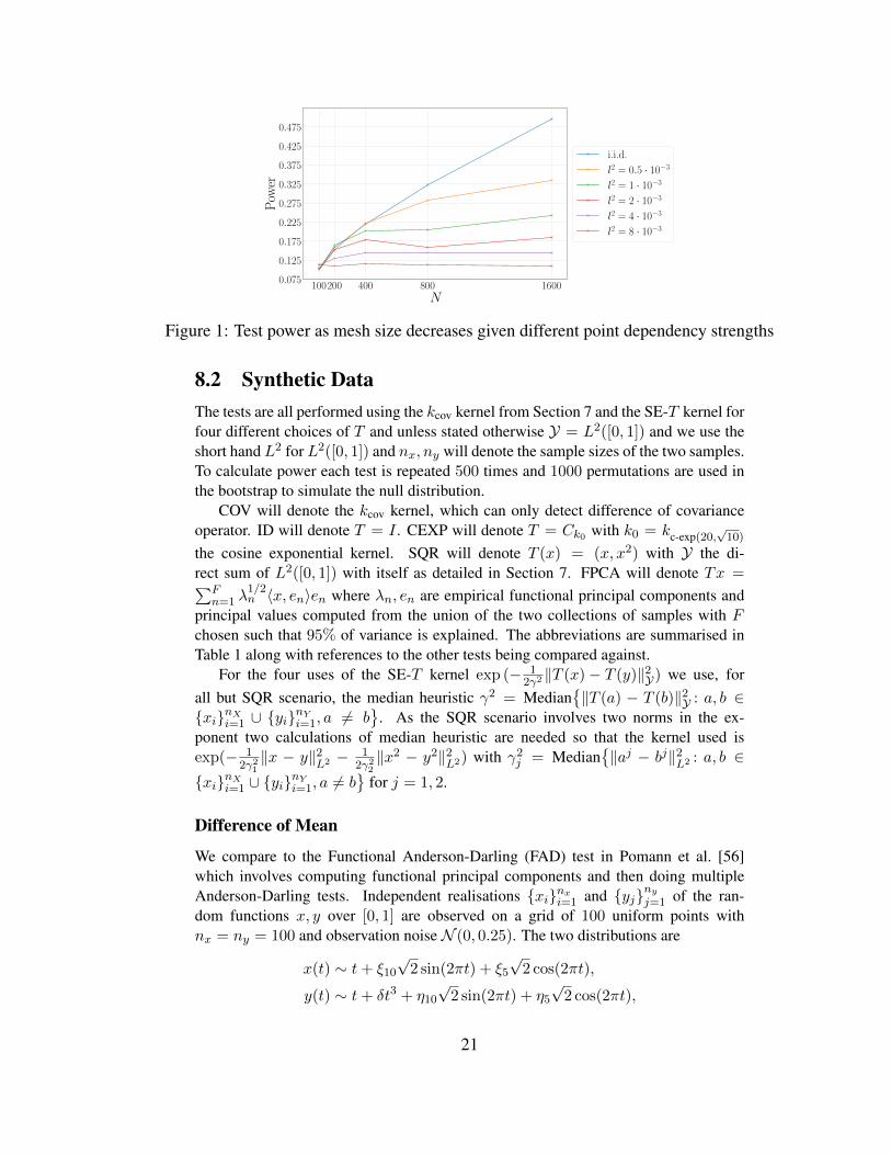
8.1 Power Scaling of Functional DataVerification of the power scaling when performing the mean shift two-sample test usingfunctional data, discussed in Section 4, is performed. Specifically we perform the two-sample test using the SE-I kernel with x ∼ GP(0, kl) and y ∼ GP(m, kl) wherem(t) = 0.05 for t ∈ [0, 1] and kl(s, t) = e−

12l2

(s−t)2 with 50 samples from eachdistribution. This is repeated 500 times to calculate power with 1000 permutationsused in the bootstrap to simulate the null. The observation points are a uniform gridon [0, 1] with N points, meaning N will be the dimension of the observed discretisedfunction vectors. The parameter l dictates the dependency of the fluctations. Small lmeans less dependency between the random function values so the covariance matrix iscloser to the identity. When the random functions are m with N (0, 1) i.i.d. corruptionthe corresponding value of l is zero which essentially means kl(x, y) = δxy. In thiscase the scaling of power is expected to follow (6) and grow asymptotically as

√N .

On the other hand if l > 0 the fluctuations within each random function are dependentand we expect scaling as (7) which does not grow asymptotically with N .

Figure 1 confirms this theory showing that power increases with a finer observationmesh only when there is no dependence in the random functions values. We see someincrease of power as the mesh gets finer for the case of small dependency however therate of increase is much smaller than the i.i.d. setting.

20

100200 400 800 1600N

0.075

0.125

0.175

0.225

0.275

0.325

0.375

0.425

0.475

Pow

er

i.i.d.

l2 = 0.5 · 10−3

l2 = 1 · 10−3

l2 = 2 · 10−3

l2 = 4 · 10−3

l2 = 8 · 10−3

Figure 1: Test power as mesh size decreases given different point dependency strengths

8.2 Synthetic DataThe tests are all performed using the kcov kernel from Section 7 and the SE-T kernel forfour different choices of T and unless stated otherwise Y = L2([0, 1]) and we use theshort hand L2 for L2([0, 1]) and nx, ny will denote the sample sizes of the two samples.To calculate power each test is repeated 500 times and 1000 permutations are used inthe bootstrap to simulate the null distribution.

COV will denote the kcov kernel, which can only detect difference of covarianceoperator. ID will denote T = I . CEXP will denote T = Ck0 with k0 = kc-exp(20,

√10)

the cosine exponential kernel. SQR will denote T (x) = (x, x2) with Y the di-rect sum of L2([0, 1]) with itself as detailed in Section 7. FPCA will denote Tx =∑F

n=1 λ1/2n 〈x, en〉en where λn, en are empirical functional principal components and

principal values computed from the union of the two collections of samples with Fchosen such that 95% of variance is explained. The abbreviations are summarised inTable 1 along with references to the other tests being compared against.

For the four uses of the SE-T kernel exp (− 12γ2‖T (x)− T (y)‖2Y) we use, for

all but SQR scenario, the median heuristic γ2 = Median‖T (a) − T (b)‖2Y : a, b ∈

xinXi=1 ∪ yinYi=1, a 6= b

. As the SQR scenario involves two norms in the ex-ponent two calculations of median heuristic are needed so that the kernel used isexp(− 1

2γ21‖x − y‖2L2 − 1

2γ22‖x2 − y2‖2L2) with γ2

j = Median‖aj − bj‖2L2 : a, b ∈

xinXi=1 ∪ yinYi=1, a 6= b

for j = 1, 2.

Difference of Mean

We compare to the Functional Anderson-Darling (FAD) test in Pomann et al. [56]which involves computing functional principal components and then doing multipleAnderson-Darling tests. Independent realisations xinxi=1 and yjnyj=1 of the ran-dom functions x, y over [0, 1] are observed on a grid of 100 uniform points withnx = ny = 100 and observation noise N (0, 0.25). The two distributions are

x(t) ∼ t+ ξ10

√2 sin(2πt) + ξ5

√2 cos(2πt),

y(t) ∼ t+ δt3 + η10

√2 sin(2πt) + η5

√2 cos(2πt),

21

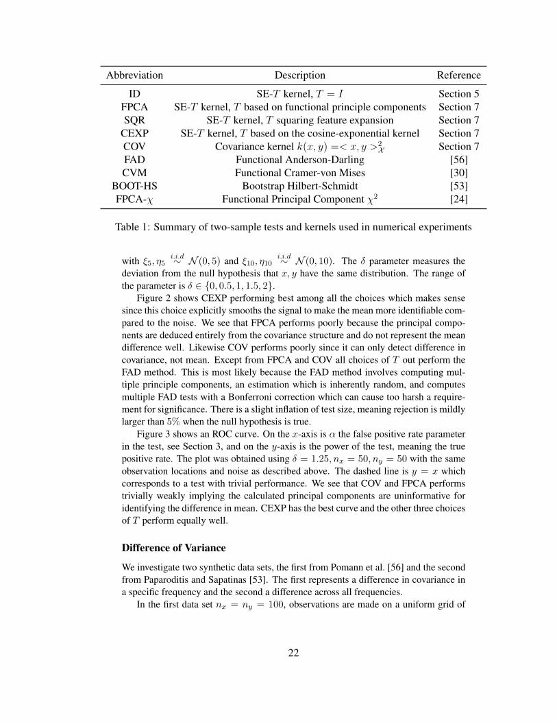
Abbreviation Description Reference

ID SE-T kernel, T = I Section 5FPCA SE-T kernel, T based on functional principle components Section 7SQR SE-T kernel, T squaring feature expansion Section 7

CEXP SE-T kernel, T based on the cosine-exponential kernel Section 7COV Covariance kernel k(x, y) =< x, y >2

X Section 7FAD Functional Anderson-Darling [56]CVM Functional Cramer-von Mises [30]

BOOT-HS Bootstrap Hilbert-Schmidt [53]FPCA-χ Functional Principal Component χ2 [24]

Table 1: Summary of two-sample tests and kernels used in numerical experiments

with ξ5, η5i.i.d∼ N (0, 5) and ξ10, η10

i.i.d∼ N (0, 10). The δ parameter measures thedeviation from the null hypothesis that x, y have the same distribution. The range ofthe parameter is δ ∈ 0, 0.5, 1, 1.5, 2.

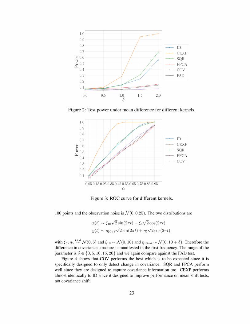
Figure 2 shows CEXP performing best among all the choices which makes sensesince this choice explicitly smooths the signal to make the mean more identifiable com-pared to the noise. We see that FPCA performs poorly because the principal compo-nents are deduced entirely from the covariance structure and do not represent the meandifference well. Likewise COV performs poorly since it can only detect difference incovariance, not mean. Except from FPCA and COV all choices of T out perform theFAD method. This is most likely because the FAD method involves computing mul-tiple principle components, an estimation which is inherently random, and computesmultiple FAD tests with a Bonferroni correction which can cause too harsh a require-ment for significance. There is a slight inflation of test size, meaning rejection is mildlylarger than 5% when the null hypothesis is true.

Figure 3 shows an ROC curve. On the x-axis is α the false positive rate parameterin the test, see Section 3, and on the y-axis is the power of the test, meaning the truepositive rate. The plot was obtained using δ = 1.25, nx = 50, ny = 50 with the sameobservation locations and noise as described above. The dashed line is y = x whichcorresponds to a test with trivial performance. We see that COV and FPCA performstrivially weakly implying the calculated principal components are uninformative foridentifying the difference in mean. CEXP has the best curve and the other three choicesof T perform equally well.

Difference of Variance

We investigate two synthetic data sets, the first from Pomann et al. [56] and the secondfrom Paparoditis and Sapatinas [53]. The first represents a difference in covariance ina specific frequency and the second a difference across all frequencies.

In the first data set nx = ny = 100, observations are made on a uniform grid of

22

0.0 0.5 1.0 1.5 2.0δ

0.1

0.2

0.3

0.4

0.5

0.6

0.7

0.8

0.9

1.0

Pow

er

ID

CEXP

SQR

FPCA

COV

FAD

Figure 2: Test power under mean difference for different kernels.

0.05 0.15 0.25 0.35 0.45 0.55 0.65 0.75 0.85 0.95α

0.1

0.2

0.3

0.4

0.5

0.6

0.7

0.8

0.9

1.0

Pow

er

ID

CEXP

SQR

FPCA

COV

Figure 3: ROC curve for different kernels.

100 points and the observation noise is N (0, 0.25). The two distributions are

x(t) ∼ ξ10

√2 sin(2πt) + ξ5

√2 cos(2πt),

y(t) ∼ η10+δ

√2 sin(2πt) + η5

√2 cos(2πt),

with ξ5, η5i.i.d∼ N (0, 5) and ξ10 ∼ N (0, 10) and η10+δ ∼ N (0, 10 + δ). Therefore the

difference in covariance structure is manifested in the first frequency. The range of theparameter is δ ∈ 0, 5, 10, 15, 20 and we again compare against the FAD test.

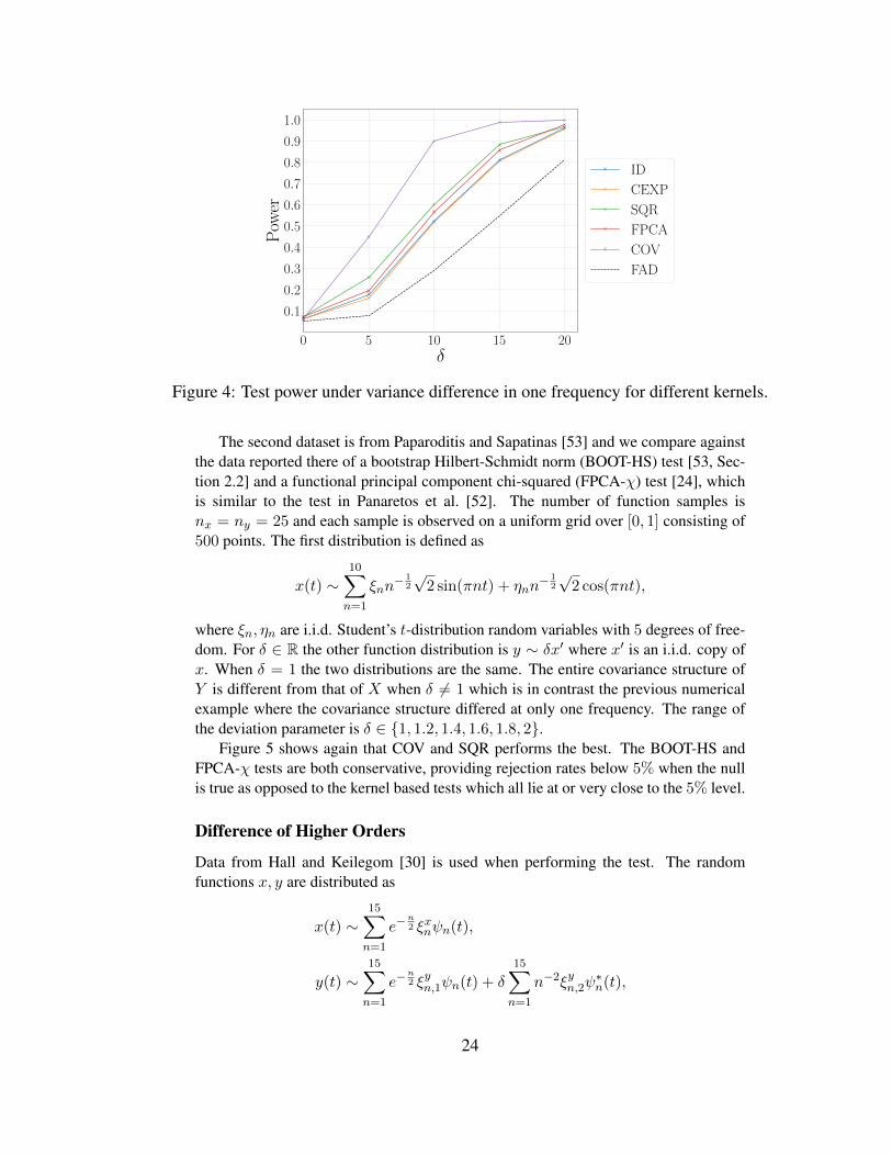
Figure 4 shows that COV performs the best which is to be expected since it isspecifically designed to only detect change in covariance. SQR and FPCA performwell since they are designed to capture covariance information too. CEXP performsalmost identically to ID since it designed to improve performance on mean shift tests,not covariance shift.

23

0 5 10 15 20δ

0.1

0.2

0.3

0.4

0.5

0.6

0.7

0.8

0.9

1.0

Pow

er

ID

CEXP

SQR

FPCA

COV

FAD

Figure 4: Test power under variance difference in one frequency for different kernels.

The second dataset is from Paparoditis and Sapatinas [53] and we compare againstthe data reported there of a bootstrap Hilbert-Schmidt norm (BOOT-HS) test [53, Sec-tion 2.2] and a functional principal component chi-squared (FPCA-χ) test [24], whichis similar to the test in Panaretos et al. [52]. The number of function samples isnx = ny = 25 and each sample is observed on a uniform grid over [0, 1] consisting of500 points. The first distribution is defined as

x(t) ∼10∑n=1

ξnn− 1

2

√2 sin(πnt) + ηnn

− 12

√2 cos(πnt),

where ξn, ηn are i.i.d. Student’s t-distribution random variables with 5 degrees of free-dom. For δ ∈ R the other function distribution is y ∼ δx′ where x′ is an i.i.d. copy ofx. When δ = 1 the two distributions are the same. The entire covariance structure ofY is different from that of X when δ 6= 1 which is in contrast the previous numericalexample where the covariance structure differed at only one frequency. The range ofthe deviation parameter is δ ∈ 1, 1.2, 1.4, 1.6, 1.8, 2.

Figure 5 shows again that COV and SQR performs the best. The BOOT-HS andFPCA-χ tests are both conservative, providing rejection rates below 5% when the nullis true as opposed to the kernel based tests which all lie at or very close to the 5% level.

Difference of Higher Orders

Data from Hall and Keilegom [30] is used when performing the test. The randomfunctions x, y are distributed as

x(t) ∼15∑n=1

e−n2 ξxnψn(t),

y(t) ∼15∑n=1

e−n2 ξyn,1ψn(t) + δ

15∑n=1

n−2ξyn,2ψ∗n(t),

24

1.0 1.2 1.4 1.6 1.8 2.0δ

0.1

0.2

0.3

0.4

0.5

0.6

0.7

0.8

0.9

1.0

Pow

er

ID

CEXP

SQR

FPCA

COV

BOOT-HS

FPCA-χ

Figure 5: Test power under variance difference across all frequencies for different kernels.

with ξxn, ξyn,1, ξ

yn,2

i.i.d∼ N (0, 1), ψ1(t) = 1, ψn(t) =√

2 sin((k − 1)πt) for n > 1 andψ∗1(t) = 1, ψ∗n(t) =

√2 cos((k − 1)π(2t− 1)) if n > 1 is even, ψ∗n(t) =

√2 sin((k −

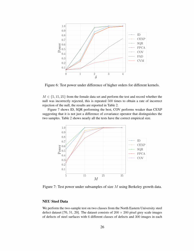
1)π(2t − 1)) if n > 1 is odd. The observation noise for x is N (0, 0.01) and for y isN (0, 0.09). The range of the parameter is δ ∈ 0, 1, 2, 3, 4 and we compare againstthe FAD test and the Cramer-von Mises test in Hall and Keilegom [30]. The numberof samples is nx = ny = 15 and for each random function 20 observation locationsare sampled randomly according to px or py with px being the uniform distribution on[0, 1] and py the distribution with density function 0.8 + 0.4t on [0, 1].

Since the data is noisy and irregularly sampled, curves were fit to the data before thetest was performed. The posterior mean of a Gaussian process with noise parameterσ2 = 0.01 was fit to each data sample using a Matern-1.5 kernel kMat(s, t) = (1 +√

3(s− t))e−√

3(s−t).Figure 6 shows that the COV, SQR perform the best with other choices of T per-

forming equally. Good power is still obtained against the existing methods despite thefunction reconstructions, validating the theoretical results of Section 6.

8.3 Real DataBerkeley Growth Data

We now perform tests on the Berkeley growth dataset which contains the height of 39male and 54 female children from age 1 to 18 and 31 locations. The data can be foundin the R package fda. We perform the two sample test on this data for the five differentchoices of T with γ chosen via the median heuristic outlined in the previous subsec-tion. To identify the effect on test performance of sample size we perform randomsubsampling of the datasets and repeat the test to calculate test power. For each samplesize M ∈ 5, 15, 25, 35 we sample M functions from each data set and perform thetest, this is repeated 500 times to calculate test power. The results are plotted in Figure7. Similarly, to investigate the size of the test we sample two disjoint subsets of size

25

0 1 2 3 4δ

0.1

0.2

0.3

0.4

0.5

0.6

0.7

0.8

0.9

1.0

Pow

er

ID

CEXP

SQR

FPCA

COV

FAD

CVM

Figure 6: Test power under difference of higher orders for different kernels.

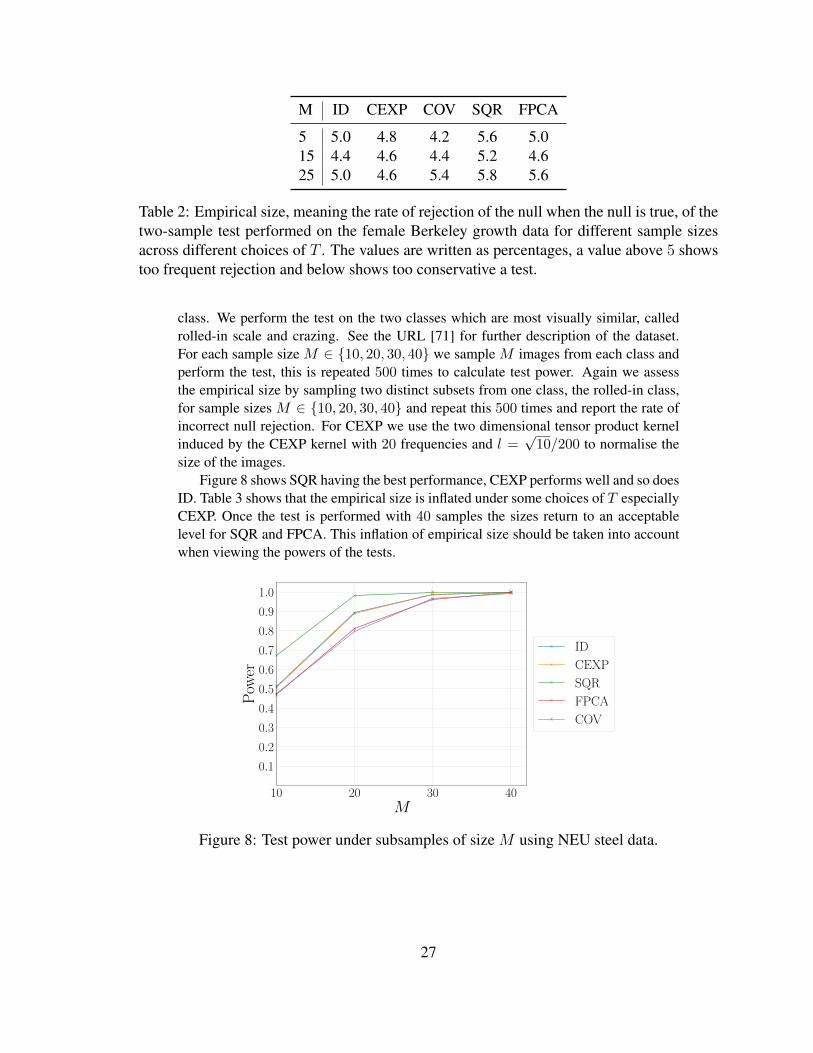
M ∈ 5, 15, 25 from the female data set and perform the test and record whether thenull was incorrectly rejected, this is repeated 500 times to obtain a rate of incorrectrejection of the null, the results are reported in Table 2.

Figure 7 shows ID, SQR performing the best, COV performs weaker than CEXPsuggesting that it is not just a difference of covariance operator that distinguishes thetwo samples. Table 2 shows nearly all the tests have the correct empirical size.

5 15 25 35M

0.1

0.2

0.3

0.4

0.5

0.6

0.7

0.8

0.9

1.0

Pow

er

ID

CEXP

SQR

FPCA

COV

Figure 7: Test power under subsamples of size M using Berkeley growth data.

NEU Steel Data

We perform the two-sample test on two classes from the North Eastern University steeldefect dataset [70, 31, 20]. The dataset consists of 200 × 200 pixel grey scale imagesof defects of steel surfaces with 6 different classes of defects and 300 images in each

26

M ID CEXP COV SQR FPCA

5 5.0 4.8 4.2 5.6 5.015 4.4 4.6 4.4 5.2 4.625 5.0 4.6 5.4 5.8 5.6

Table 2: Empirical size, meaning the rate of rejection of the null when the null is true, of thetwo-sample test performed on the female Berkeley growth data for different sample sizesacross different choices of T . The values are written as percentages, a value above 5 showstoo frequent rejection and below shows too conservative a test.

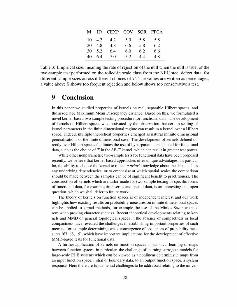
class. We perform the test on the two classes which are most visually similar, calledrolled-in scale and crazing. See the URL [71] for further description of the dataset.For each sample size M ∈ 10, 20, 30, 40 we sample M images from each class andperform the test, this is repeated 500 times to calculate test power. Again we assessthe empirical size by sampling two distinct subsets from one class, the rolled-in class,for sample sizes M ∈ 10, 20, 30, 40 and repeat this 500 times and report the rate ofincorrect null rejection. For CEXP we use the two dimensional tensor product kernelinduced by the CEXP kernel with 20 frequencies and l =

√10/200 to normalise the

size of the images.Figure 8 shows SQR having the best performance, CEXP performs well and so does

ID. Table 3 shows that the empirical size is inflated under some choices of T especiallyCEXP. Once the test is performed with 40 samples the sizes return to an acceptablelevel for SQR and FPCA. This inflation of empirical size should be taken into accountwhen viewing the powers of the tests.

10 20 30 40M

0.1

0.2

0.3

0.4

0.5

0.6

0.7

0.8

0.9

1.0

Pow

er

ID

CEXP

SQR

FPCA

COV

Figure 8: Test power under subsamples of size M using NEU steel data.

27

M ID CEXP COV SQR FPCA

10 4.2 4.2 5.0 5.8 5.820 4.8 4.8 6.6 5.8 6.230 5.2 6.4 6.0 6.2 6.640 6.4 7.0 5.2 4.4 4.8

Table 3: Empirical size, meaning the rate of rejection of the null when the null is true, of thetwo-sample test performed on the rolled-in scale class from the NEU steel defect data, fordifferent sample sizes across different choices of T . The values are written as percentages,a value above 5 shows too frequent rejection and below shows too conservative a test.

9 ConclusionIn this paper we studied properties of kernels on real, separable Hilbert spaces, andthe associated Maximum Mean Discrepancy distance. Based on this, we formulated anovel kernel-based two-sample testing procedure for functional data. The developmentof kernels on Hilbert spaces was motivated by the observation that certain scaling ofkernel parameters in the finite dimensional regime can result in a kernel over a Hilbertspace. Indeed, multiple theoretical properties emerged as natural infinite dimensionalgeneralisations of the finite dimensional case. The development of kernels defined di-rectly over Hilbert spaces facilitates the use of hyperparameters adapted for functionaldata, such as the choice of T in the SE-T kernel, which can result in greater test power.

While other nonparametric two-sample tests for functional data have been proposedrecently, we believe that kernel-based approaches offer unique advantages. In particu-lar, the ability to choose the kernel to reflect a priori knowledge about the data, such asany underlying dependencies, or to emphasise at which spatial scales the comparisonshould be made between the samples can be of significant benefit to practitioners. Theconstruction of kernels which are tailor-made for two-sample testing of specific formsof functional data, for example time series and spatial data, is an interesting and openquestion, which we shall defer to future work.

The theory of kernels on function spaces is of independent interest and our workhighlights how existing results on probability measures on infinite dimensional spacescan be applied to kernel methods, for example the use of the Minlos-Sazanov theo-rem when proving characteristicness. Recent theoretical developments relating to ker-nels and MMD on general topological spaces in the absence of compactness or localcompactness have revealed the challenges in establishing important properties of suchmetrics, for example determining weak convergence of sequences of probability mea-sures [67, 68, 15], which have important implications for the development of effectiveMMD-based tests for functional data.

A further application of kernels on function spaces is statistical learning of mapsbetween function spaces, in particular, the challenge of learning surrogate models forlarge-scale PDE systems which can be viewed as a nonlinear deterministic maps froman input function space, initial or boundary data, to an output function space, a systemresponse. Here there are fundamental challenges to be addressed relating to the univer-

28

sality properties of such kernels. Preliminary work in Nelsen and Stuart [50] indicatesthat this is a promising direction of research.

AcknowledgmentsGW was supported by an EPSRC Industrial CASE award [18000171] in partnershipwith Shell UK Ltd. AD was supported by the Lloyds Register Foundation Programmeon Data Centric Engineering and by The Alan Turing Institute under the EPSRC grant[EP/N510129/1]. We thank Sebastian Vollmer for helpful comments.

References[1] S. Albeverio and S. Mazzucchi. An introduction to infinite-dimensional oscillatory and probabilistic integrals. In

Stochastic Analysis: A Series of Lectures, pages 1–54. Springer Basel, 2015.[2] A. Aue, G. Rice, and O. Sonmez. Detecting and dating structural breaks in functional data without dimension

reduction. Journal of the Royal Statistical Society: Series B (Statistical Methodology), 80(3):509–529, 2018.[3] F. Bach. On the equivalence between kernel quadrature rules and random feature expansions. The Journal of

Machine Learning Research, 18(1):714–751, 2017.[4] M. Benko, W. Hardle, and A. Kneip. Common functional principal components. The Annals of Statistics, 37(1):

1–34, 2009.[5] C. Berg, J. P. R. Christensen, and P. Ressel. Harmonic Analysis on Semigroups. Springer New York, 1984.[6] A. Berlinet and C. Thomas-Agnan. Reproducing Kernel Hilbert Spaces in Probability and Statistics. Springer

US, 2004.[7] J. R. Berrendero, B. Bueno-Larraz, and A. Cuevas. On Mahalanobis distance in functional settings. Journal of

Machine Learning Research, 21(9):1–33, 2020.[8] P. Billingsley. Weak Convergence of Measures. Society for Industrial and Applied Mathematics, 1971.[9] K. M. Borgwardt, A. Gretton, M. J. Rasch, H.-P. Kriegel, B. Scholkopf, and A. J. Smola. Integrating structured

biological data by kernel maximum mean discrepancy. Bioinformatics, 22(14):49–57, 2006.[10] B. Bucchia and M. Wendler. Change-point detection and bootstrap for Hilbert space valued random fields.

Journal of Multivariate Analysis, 155:344–368, 2017.[11] A. Cabana, A. M. Estrada, J. Pena, and A. J. Quiroz. Permutation tests in the two-sample problem for functional

data. In Functional Statistics and Related Fields, pages 77–85. Springer, 2017.[12] C. Carmeli, E. de Vito, A. Toigo, and V. Umanita. Vector valued reproducing kernel hilbert spaces and univer-

sality. Analysis and Applications, 08(01):19–61, Jan. 2010.[13] S. Chakraborty and X. Zhang. A new framework for distance and kernel-based metrics in high dimensions.

arXiv:1909.13469, 2019.[14] H. Chen, P. T. Reiss, and T. Tarpey. Optimally weighted L2 distance for functional data. Biometrics, 70(3):

516–525, 2014.[15] I. Chevyrev and H. Oberhauser. Signature moments to characterize laws of stochastic processes.

arXiv:1810.10971, 2018.[16] A. Christmann and I. Steinwart. Universal kernels on non-standard input spaces. Advances in Neural Information

Processing Systems 23, pages 406–414, 2010.[17] A. Cuevas. A partial overview of the theory of statistics with functional data. Journal of Statistical Planning and

Inference, 147:1–23, 2014.[18] G. Da Prato. An Introduction to Infinite-Dimensional Analysis. Springer Berlin Heidelberg, 2006.[19] G. Da Prato and J. Zabczyk. Second Order Partial Differential Equations in Hilbert Spaces. Cambridge Univer-

sity Press, 2002.[20] H. Dong, K. Song, Y. He, J. Xu, Y. Yan, and Q. Meng. PGA-Net: pyramid feature fusion and global context

attention network for automated surface defect detection. IEEE Transactions on Industrial Informatics, 2019.[21] S. N. Ethier and T. G. Kurtz, editors. Markov Processes. John Wiley & Sons, Inc., 1986.[22] G. Fasshauer and M. McCourt. Kernel-based Approximation Methods using MATLAB. World Scientific, June

2014.[23] F. Ferraty and P. Vieu. Curves discrimination: a nonparametric functional approach. Computational Statistics &

Data Analysis, 44(1-2):161–173, 2003.[24] S. Fremdt, J. G. Steinbach, L. Horvath, and P. Kokoszka. Testing the equality of covariance operators in functional

samples. Scandinavian Journal of Statistics, 40(1):138–152, 2012.[25] J. H. Friedman and L. C. Rafsky. Multivariate generalizations of the Wald-Wolfowitz and Smirnov two-sample

tests. The Annals of Statistics, pages 697–717, 1979.[26] T. Gartner. A survey of kernels for structured data. ACM SIGKDD Explorations Newsletter, 5(1):49, 2003.

29

[27] A. Gretton, K. Borgwardt, M. Rasch, B. Scholkopf, and A. J. Smola. A kernel method for the two-sample-problem. Advances in Neural Information Processing Systems 19, pages 513–520, 2007.

[28] A. Gretton, K. M. Borgwardt, M. J. Rasch, B. Scholkopf, and A. Smola. A kernel two-sample test. Journal ofMachine Learning Research, 13(1):723–773, 2012.

[29] A. Gretton, D. Sejdinovic, H. Strathmann, S. Balakrishnan, M. Pontil, K. Fukumizu, and B. K. Sriperumbudur.Optimal kernel choice for large-scale two-sample tests. Advances in Neural Information Processing Systems 25,pages 1205–1213, 2012.

[30] P. Hall and I. V. Keilegom. Two-sample tests in functional data analysis starting from discrete data. StatisticaSinica, 17(4):1511–1531, 2007. ISSN 10170405, 19968507.

[31] Y. He, K. Song, Q. Meng, and Y. Yan. An end-to-end steel surface defect detection approach via fusing multiplehierarchical features. IEEE Transactions on Instrumentation and Measurement, 69(4):1493–1504, 2020.

[32] L. Horvath and P. Kokoszka. Inference For Functional Data With Applications. Springer Science & BusinessMedia, 2012.

[33] L. Horvath, P. Kokoszka, and R. Reeder. Estimation of the mean of functional time series and a two-sampleproblem. Journal of the Royal Statistical Society: Series B (Statistical Methodology), 75(1):103–122, 2012.

[34] L. Horvath, P. Kokoszka, and G. Rice. Testing stationarity of functional time series. Journal of Econometrics,179(1):66–82, 2014.

[35] T. Hsing and R. Eubank. Theoretical Foundations of Functional Data Analysis, with an Introduction to LinearOperators. John Wiley & Sons, Ltd, 2015.

[36] W. Jitkrittum, W. Xu, Z. Szabo, K. Fukumizu, and A. Gretton. A linear-time kernel goodness-of-fit test. Advancesin Neural Information Processing Systems 30, pages 262–271, 2017.

[37] H. Kadri, E. Duflos, P. Preux, S. Canu, A. Rakotomamonjy, and J. Audiffren. Operator-valued kernels for learningfrom functional response data. Journal of Machine Learning Research, 17(20):1–54, 2016.

[38] M. Kanagawa, P. Hennig, D. Sejdinovic, and B. K. Sriperumbudur. Gaussian processes and kernel methods: Areview on connections and equivalences. arXiv:1807.02582, 2018.

[39] A. S. Kechris. Classical Descriptive Set Theory. Springer New York, 1995.[40] P. Kidger, P. Bonnier, I. Perez Arribas, C. Salvi, and T. Lyons. Deep signature transforms. In Advances in Neural

Information Processing Systems 32, pages 3105–3115. Curran Associates, Inc., 2019.[41] A. Kolmogorov-Smirnov, A. Kolmogorov, and M. Kolmogorov. Sulla determinazione empirica di uma legge di

distribuzione. Giornale dell’Istituto Italiano degli Attuari, 1933.[42] F. Liu, W. Xu, J. Lu, G. Zhang, A. Gretton, and D. J. Sutherland. Learning deep kernels for non-parametric

two-sample tests. In Proceedings of the 37th International Conference on Machine Learning, 2020.[43] M. Lopes, L. Jacob, and M. J. Wainwright. A more powerful two-sample test in high dimensions using random

projection. Advances in Neural Information Processing Systems, pages 1206–1214, 2011.[44] S. Maniglia and A. Rhandi. Gaussian measures on separable hilbert spaces and applications, 2004.[45] K. Mardia and I. Dryden. The statistical analysis of shape data. Biometrika, 76(2):271–281, 1989.[46] H. Q. Minh. Some properties of Gaussian reproducing kernel Hilbert spaces and their implications for function

approximation and learning theory. Constructive Approximation, 32(2):307–338, 2009.[47] K. Muandet, K. Fukumizu, B. Sriperumbudur, and B. Scholkopf. Kernel mean embedding of distributions: A

review and beyond. Foundations and Trends® in Machine Learning, 10(1-2):1–141, 2017.[48] A. Muller. Integral probability metrics and their generating classes of functions. Advances in Applied Probability,

29(2):429–443, 1997.[49] F. J. Narcowich, J. D. Ward, and H. Wendland. Sobolev error estimates and a Bernstein inequality for scattered

data interpolation via radial basis functions. Constructive Approximation, 24(2):175–186, 2006.[50] N. H. Nelsen and A. M. Stuart. The random feature model for input-output maps between Banach spaces.

arXiv:2005.10224, 2020.[51] I. Nourdin and G. Peccati. Normal Approximations with Malliavin Calculus. Cambridge University Press, 2009.[52] V. M. Panaretos, D. Kraus, and J. H. Maddocks. Second-order comparison of Gaussian random functions and the

geometry of DNA minicircles. Journal of the American Statistical Association, 105(490):670–682, 2010.[53] E. Paparoditis and T. Sapatinas. Bootstrap-based testing of equality of mean functions or equality of covariance

operators for functional data. Biometrika, 103(3):727–733, 2016.[54] V. I. Paulsen and M. Raghupathi. An introduction to the theory of reproducing kernel Hilbert spaces, volume 152

of Cambridge Studies in Advanced Mathematics. Cambridge University Press, Cambridge, 2016.[55] B. Pelletier. Kernel density estimation on riemannian manifolds. Statistics & Probability Letters, 73(3):297–304,

2005.[56] G.-M. Pomann, A.-M. Staicu, and S. Ghosh. A two-sample distribution-free test for functional data with appli-

cation to a diffusion tensor imaging study of multiple sclerosis. Journal of the Royal Statistical Society: Series C(Applied Statistics), 65(3):395–414, Jan. 2016.

[57] A. Rahimi and B. Recht. Random features for large-scale kernel machines. Advances in Neural InformationProcessing Systems 20, pages 1177–1184, 2008.

[58] A. Ramdas, S. J. Reddi, B. Poczos, A. Singh, and L. Wasserman. On the decreasing power of kernel anddistance based nonparametric hypothesis tests in high dimensions. In Twenty-Ninth AAAI Conference on ArtificialIntelligence, 2015.

[59] A. Ramdas, S. J. Reddi, B. Poczos, A. R. Singh, and L. A. Wasserman. On the high-dimensional power of

30

linear-time kernel two-sample testing under mean-difference alternatives. In 18th International Conference onArtificial Intelligence and Statistics, 2015.

[60] C. Rasmussen and C. Williams. Gaussian Processes for Machine Learning. MIT Press, 2006.[61] S. Saitoh and Y. Sawano. Theory of reproducing kernels and applications. Springer, 2016.[62] P. Schmid. On the Kolmogorov and Smirnov limit theorems for discontinuous distribution functions. The Annals

of Mathematical Statistics, 29(4):1011–1027, 1958.[63] I. J. Schoenberg. Metric spaces and completely monotone functions. The Annals of Mathematics, 39(4):811,

1938.[64] D. Sejdinovic, B. Sriperumbudur, A. Gretton, and K. Fukumizu. Equivalence of distance-based and RKHS-based

statistics in hypothesis testing. The Annals of Statistics, 41(5):2263–2291, 2013.[65] R. J. Serfling. Approximation Theorems of Mathematical Statistics. John Wiley & Sons, Inc., Nov. 1980.[66] J. Shawe-Taylor and N. Cristianini. Kernel Methods for Pattern Analysis. Cambridge University Press, 2004.[67] C.-J. Simon-Gabriel and B. Scholkopf. Kernel distribution embeddings: Universal kernels, characteristic kernels

and kernel metrics on distributions. Journal of Machine Learning Research, 19(44):1–29, 2018.[68] C.-J. Simon-Gabriel, A. Barp, and L. Mackey. Metrizing weak convergence with Maximum Mean Discrepancies.

arXiv:2006.09268, 2020.[69] N. Smirnov. Table for estimating the goodness of fit of empirical distributions. The Annals of Mathematical

Statistics, 19(2):279–281, 1948.[70] K. Song and Y. Yan. A noise robust method based on completed local binary patterns for hot-rolled steel strip

surface defects. Applied Surface Science, 285:858–864, 2013.[71] K. Song and Y. Yan. NEU Steel Dataset Description. http://faculty.neu.edu.cn/yunhyan/NEU_

surface_defect_database.html, 2020. Last accessed 29/07/2020.[72] B. K. Sriperumbudur, A. Gretton, K. Fukumizu, B. Scholkopf, and G. R. Lanckriet. Hilbert space embeddings

and metrics on probability measures. Journal of Machine Learning Research, 11:1517–1561, 2010. ISSN 1532-4435.

[73] B. K. Sriperumbudur, K. Fukumizu, and G. R. G. Lanckriet. Universality, characteristic kernels and RKHSembedding of measures. Journal of Machine Learning Research, 12:2389–2410, 2011. ISSN 1532-4435.

[74] I. Steinwart and A. Christmann. Support Vector Machines. Springer, 2008.[75] I. Steinwart and C. Scovel. Mercer’s theorem on general domains: On the interaction between measures, kernels,

and RKHSs. Constructive Approximation, 35(3):363–417, 2012.[76] T. Sullivan. Introduction to Uncertainty Quantification. Springer International Publishing, 2015.[77] D. J. Sutherland. Unbiased estimators for the variance of MMD estimators. arXiv:1906.02104, 2019.[78] D. J. Sutherland, H.-Y. Tung, H. Strathmann, S. De, A. Ramdas, A. Smola, and A. Gretton. Generative models and

model criticism via optimized maximum mean discrepancy. In Proceedings of the 8th International Conferenceon Learning Representations, 2016.

[79] G. J. Szekely. E-statistics: The energy of statistical samples. Bowling Green State University, Department ofMathematics and Statistics Technical Report, 3(05):1–18, 2003.

[80] G. J. Szekely and M. L. Rizzo. Testing for equal distributions in high dimension. InterStat, 5(16.10):1249–1272,2004.

[81] N. N. Vakhania, V. I. Tarieladze, and S. A. Chobanyan. Probability Distributions on Banach Spaces. SpringerNetherlands, 1987.

[82] A. W. van der Vaart and J. H. van Zanten. Information rates of nonparametric Gaussian process methods. Journalof Machine Learning Research, 12:2095–2119, 2011.

[83] G. Wahba. Spline models for observational data, volume 59. Siam, 1990.[84] A. Wald and J. Wolfowitz. On a test whether two samples are from the same distribution. The Annals of

Mathematical Statistics, 11:147–162, 1940.[85] H. Wendland. Scattered Data Approximation. Cambridge University Press, 2005.[86] W. J. Wilkinson. Gaussian Process Modelling for Audio Signals. PhD thesis, Queen Mary Univeristy London,

2019.[87] G. Wynne, F.-X. Briol, and M. Girolami. Convergence guarantees for Gaussian process means with misspecified

likelihoods and smoothness. arXiv:2001.10818, 2020.[88] H. Zhang, Y. Xu, and Q. Zhang. Refinement of operator-valued reproducing kernels. Journal of Machine

Learning Research, 13(4):91–136, 2012.[89] J.-T. Zhang, X. Liang, and S. Xiao. On the two-sample Behrens-Fisher problem for functional data. Journal of

Statistical Theory and Practice, 4(4):571–587, 2010.[90] C. Zhu, S. Yao, X. Zhang, and X. Shao. Distance-based and RKHS-based dependence metrics in high dimension.

Annals of Statistics, 2019. To appear.

31

A Appendix

A.1 Bochner and Minlos-Sazanov TheoremBochner’s theorem provides an exact relationship between continuous, translation in-variant kernels on Rd, meaning k(x, y) = φ(x − y) for some continuous φ, and theFourier transforms of finite Borel measures on Rd. For a proof see Wendland [85,Theorem 6.6].

Theorem 10 (Bochner). A continuous function φ : Rd → C is positive definite if andonly if it is the Fourier transform of a finite Borel measure µφ on Rd

µφ(x) :=

∫Rdeix

T ydµφ(y) = φ(x).

Bochner’s theorem does not continue to hold in infinite dimensions, for example thekernel k(x, y) = e−

12‖x−y‖2X when X is an infinite dimensional, real, separable Hilbert

space is not the Fourier transform of a finite Borel measure on X [44, Proposition1.2.11]. Instead, a stronger continuity property is required, this is the content of theMinlos-Sazanov theorem. For a proof see [44, Theorem 1.1.5] or Vakhania et al. [81,Theorem VI.1.1].

Theorem 11 (Minlos-Sazanov). LetX be a real, seperable Hilbert space and φ : X →C a positive definite function on X then the following are equivalent

1. φ is the Fourier transform of a finite Borel measure on X2. There exists C ∈ L+

1 (X ) such that φ is continuous with respect to the norminduced by C given by ‖x‖2C = 〈Cx, x〉X .

The existence of such an operator is a much stronger continuity property than stan-dard continuity on X and will be crucial in the proof of Theorem 12, one of our mainresults. To see that continuity with respect to such a C is stronger than usual conti-nuity consider the following example. Fix any ε > 0 and assume we only know thatφ : X → R is continuous and for simplicity assume that φ(0) = 1, then we know thereexists some δ > 0 such that ‖x‖X < δ implies |φ(x)−1| < εmeaning we have controlof φ(x) over the bounded set ‖x‖X < δ. On the other hand, if φ is continuous withrespect to ‖·‖C for some C ∈ L+

1 (X ) then we know there exists some δ′ > 0 such that‖x‖C < δ′ implies |φ(x)− 1| < ε so we have control of φ(x) over the unbounded set‖x‖C < δ′. To see this set is unbounded let λn, en∞n=1 be the orthonormal eigen-system of C and for n ∈ N let yn = δ′en

2λnif λn > 0 otherwise yn = nen, then since

C ∈ L+1 (X ) we know λn → 0 so ‖yn‖X → ∞. Since we used elements from the

eigensystem it is clear that ‖yn‖C ≤ δ′/2. Therefore we have constructed a subset ofthe ball with respect to ‖·‖C of radius δ′ that has unbounded norm.

A.2 Proofs for Section 4Proof of Proposition 1. We begin by outlining the scaling that occurs for each of thetwo cases. For economy of notation we set γ = γN . If k0(s, t) = δst then Tr(Σi) = N

32

for all i ∈ N and 〈mN ,ΣmN 〉 = ‖mN‖22 = Θ(N) by the Riemann scaling. If k0

is continuous and bounded then Tr(Σi) = Θ(N i) since N−iTr(Σi) → Tr(Cik0) and〈mN ,Σ

imN 〉 = Θ(N i+1) since N−(i+1)〈mN ,ΣimN 〉 →

∫D∫Dm(s)Cik0m(t)dsdt.

We shall outline the proof of the result in the second case, the proof for the firstcase is entirely analogous and is completed by substituting the above scaling resultswhere appropriate. Throughout this proof we shall repeatedly use the following Taylorseries approximation, for a positive definite matrix Σ ∈ RN×N , based on the classicalGirard-Waring formulas.

det(I + εΣ) = 1 + εTr(Σ) +ε2

2R1(s)

= 1 + εTr(Σ) +ε2

2(Tr(Σ)2 − Tr(Σ2)) +

ε3

6R2(s′),

for some 0 < s, s′ ≤ ε where

R1(s) =

(∑ λi(1 + sλi)

)2

− det(I + sΣ)∑ λ2

i

(1 + sλi)2,

and

R2(s) =− 2(1 + det(I + sΣ))∑ λi

(1 + sλi)

∑ λ2i

(1 + sλi)2

+ 2 det(I + sΣ)∑ λ3

i

(1 + sλi)3,

where λ1, . . . , λN are the eigenvalues of Σ. We may bound these remainders

R1(s) ≤(∑ λi

(1 + sλi)

)2

≤ Tr(Σ)2 = O(N2),

and

R2(s) ≤ 2 det(I + sΣ)∑ λ3

i

(1 + sλi)3≤ 2eεTr(Σ)Tr(Σ3).

In our scenario ε = γ−2 = O(N−2α) = o(N−1) therefore eεTr(Σ) is bounded sinceTr(Σ) = O(N). Finally, Tr(Σ3) = O(N3) thereforeR2(s) = O(N3). Setting T = 1

γ Iand R = S = Σ in Corollary 3 and applying the above Taylor expansion along withthe expansions for x−1/2 and (I + εΣ)−1 with Lagrange remainder term

MMD2k(P,Q) = 2 det(I + 2Σ/γ2)−

12

(1− e−

12γ2〈(I+2Σ/γ2)−1µ,µ〉

)=

(1 +

1

γ2r1

)(1

γ2

⟨(I + 2Σ/γ2)−1µ, µ

⟩+

1

γ4r2

)=

(1 +

1

γ2r1

)(1

γ2〈µ, µ〉+

1

γ4r2 +

1

γ4r3

),

where r1, r2, r3 are remainder terms.

33

To leading order r1/γ2 = O(N1−2α), r2/γ

4 = O(N2−4α), r3/γ4 = O(N2−4α)

so it follows that MMD2k(P,Q) = γ−2‖mN‖2 +r(N) where, to leading order, r(N) =

O(N2−4α). We now consider the denominator. To this end, applying Theorem 8 withT = γ−1I and S = Σ we obtain

ξ2 = 2 det(I + 4Σ/γ2)−12

(1 + e

− 1γ2〈µ,(I+4Σ/γ2)−1µ〉

)− 2 det(I + 2Σ/γ2)−1(1 + e

− 1γ2〈µ(I+2Σ/γ2)−1µ〉 − 4e

− 12γ2〈µ(I+2Σ/γ2)−1µ〉

)

− 8 det((I + Σ/γ2)(I + 3Σ/γ2))−1/2e− 1

2γ2〈µ,(I+2Σ/γ2)(I+3Σ/γ2)−1(I+Σ/γ2)−1µ〉

.

We split this into two terms, ξ2 = A1 +A2, where

A1 = 4 det(I + 4Σ/γ2)−12 + 4 det(I + 2Σ/γ2)−1

− 8 det((I + Σ/γ2)(I + 3Σ/γ2))−1/2,

and

A2 = 2 det(I + 4Σ/γ2)−12

(−1 + e

− 1γ2〈µ,(I+4Σ/γ2)−1µ〉

)− 2 det(I + 2Σ/γ2)−1(3 + e

− 1γ2〈µ(I+2Σ/γ2)−1µ〉 − 4e

− 12γ2〈µ(I+2Σ/γ2)−1µ〉

)

− 8 det((I + Σ/γ2)(I + 3Σ/γ2))−1/2

· (−1 + e− 1

2γ2〈µ,(I+2Σ/γ2)(I+3Σ/γ2)−1(I+Σ/γ2)−1µ〉

).

Applying Taylor’s theorem for the determinant and exponential terms we obtain:

A1 = 4

[1− 2

γ2Tr(Σ) +

2

γ4(Tr(Σ))2 +

4

γ4Tr(Σ2) + r1

]+ 4

[1− 2

γ2Tr(Σ) +

2

γ4(Tr(Σ))2 +

2

γ4Tr(Σ2) + r2

]− 8

[1− 1

2γ2Tr(Σ) +

1

8γ4Tr(Σ)2 +

1

4γ4Tr(Σ2) + r3

]×[1− 3

2γ2Tr(Σ) +

9

8γ4(Tr(Σ))2 +

9

4γ4Tr(Σ2) + r4

],

where to leading order r1, r2, r3, r4 = O(N3−6α + N4−8α). After simplification weobtain A1 = 4

γ4Tr(Σ2) + r(N) where r(N) = O(N3−6α). Similarly writing A2 =

B1 +B2 +B3, we obtain:

B1 =2

γ2(1− 2Tr(Σ)/γ2 + r5)

(−〈µ, µ〉+

4

γ2〈µ,Σµ〉+

1

2γ2〈µ, µ〉2 + r6

),

B2 = − 2

γ2(1− 2Tr(Σ)/γ2 + r7)

(〈µ, µ〉 − 2

γ2〈µ,Σµ〉+ r8

),

B3 = − 8

γ2

(1− 2Tr(Σ)/γ2 + r9

)(−1

2〈µ, µ〉+

1

γ2〈µ,Σµ〉+

1

8γ2〈µ, µ〉2 + r10

),

34

where r5, . . . , r10 are remainder terms which satisfy ri = O(N3−6α +N4−8α) fori = 5, . . . , 10. Expanding B1 + B2 + B3 and collecting into powers of γ, we see thatthe constant terms and the terms with denominator γ2 cancel out. Collecting terms withγ4 denominator givesA2 = 4

γ4〈µ,Σµ〉+r(N) where r(d) = O(d3−6α) is a remainder

term containing the higher order terms. Combining the leading order expressions forA1 and A2, and collecting together the remainder terms we obtain

MMD2k(P,Q)√ξ2

=‖µ‖22/γ2 + r(N)√

4Tr(Σ2)/γ4 + 4〈µ,Σµ〉/γ4 + r′(N),

where r(N) = O(N2−4α) and r′(N) = O(N3−6α) It follows that

MMD2k(P,Q)√ξ2

=‖µ‖22√

4Tr(Σ2) + 4〈µ,Σµ〉

1 + r(N)‖µ‖22/γ2√

1 + r′(N)4Tr(Σ2)/γ4+4〈µ,Σµ〉/γ4

. (11)

As discussed at the start of the proof ‖mN‖22 = Θ(N) and Tr(Σ2), 〈mN ,ΣmN 〉 =Θ(N2) meaning that γ2r(N)/‖mN‖22 = O(N1−2α) and so converges to zero. Like-wise the fraction in the square root in the denominator converges to zero, meaning theterm in the brackets of (11) converge to 1 as N → ∞, yielding the advertised resultonce numerator and denominator is divided by N since

N−2Tr(Σ2)→∫D

∫Dk0(s, t)dsdt = ‖Ck‖2HS ,

N−2〈mN ,ΣmN 〉 →∫D

∫Dm(s)k0(s, t)m(t)dsdt = ‖C1/2

k m‖2L2(D).

For the case of identity matrix substituting the corresponding scaling ofTr(Σ2), 〈mN ,ΣmN 〉 in the relevant places will produce the result.

Proof of Lemma 1. We use the standard fact that for a real valued random variables ηthe following inequality holds |E[η]−Median[η]| ≤ Var[η]

12 and we will be using this

inequality on ‖x−y‖22 where x ∼ P, y ∼ Q. For economy of notation let µ = µ1−µ2

and Σ = Σ1 + Σ2. Using standard Gaussian integral identities we obtain

E[‖x− y‖22]2 = (Tr(Σ) + ‖µ‖22)2,

E[‖x− y‖42] = 2Tr(Σ2) + 4〈µ,Σµ〉+ (Tr(Σ) + ‖µ‖22)2,

therefore

Var[‖x− y‖22] = E[‖x− y‖42]− E[‖x− y‖22]2 = 2Tr(Σ)2 + 4‖µ‖22Tr(Σ).

Substituting into the inequality at the start of the proof∣∣∣∣Median[‖x− y‖22]

E[‖x− y‖22]− 1

∣∣∣∣2 ≤ 2Tr(Σ)2 + 4‖µ‖22Tr(Σ)

(Tr(Σ) + ‖µ‖22)2= 2

(1− ‖µ‖42

(Tr(Σ) + ‖µ‖22)2

),

which completes the first part of the proof. The special case follows from dividing thenumerator and denominator of the fraction in the right hand side by N2 and using theassumption that the kernels are continuous and the mesh satisfies the Riemann scalingproperty. Writing mN for the discretised version of m1 − m2 gives N−2‖mN‖42 →‖m1−m2‖2L2(D), N

−1Tr(Σ)→ Tr(Ck1 +Ck2), N−1‖mN‖22 → ‖m1−m2‖2L2(D).

35

A.3 Proofs for Section 5Lemma 2. The SE-T function is a kernel.

Proof of Lemma 2. Consider first the case T = I , it is shown in Schoenberg [63,Theorem 3] that if k(x, y) = φ(‖x − y‖2Y) for φ a completely monotone functionthen k is positive definite on Y and it is well known that e−ax is such a functionfor a > 0 therefore kI is a kernel. Now take kT to be the SE-T kernel then forany N ∈ N, anNn=1 ⊂ R, xnNn=1 ⊂ X we have

∑Nn,m=1 anamkT (xn, xm) =∑N

n,m=1 anamkI(T (xn), T (xm)) ≥ 0

Proof of Theorem 2. This proof uses the argument of Minh [46, Theorem 1]. The planis to first show the function space stated in the theorem is an RKHS and that the kernelis the SE-T kernel so by uniqueness of kernel for RKHS we are done. This is doneusing the Aronszajn theorem [46, Theorem 9] which identifies the kernel as an infinitesum of basis functions, see also Paulsen and Raghupathi [54, Theorem 2.4].

First we prove thatHkT (X ) is a separable Hilbert space. That it is an inner productspace is clear from the definition of the inner product and the assumption that λn > 0for all n ∈ N. The definition of the inner product means completeness of HkT (X )equivalent to completeness of the weighted l2 space given by

l2λ(Γ) =

(wγ)γ∈Γ : ‖(wγ)γ∈Γ‖2l2λ(Γ):=∑γ∈Γ

γ!

λγw2γ <∞

which can be easily seen to be complete since Γ is countable and γ!/λγ is positive forall γ ∈ Γ. To see thatHkT (X ) is separable observe that from the definition of the innerproduct, the countable set of functions φγ(x) =

√λγ/γ!e−

12‖Tx‖2X xγ is orthonormal

and spansHkT (X ) hence is an orthonormal basis.Next we prove that HkT (X ) is an RKHS. Expanding the kernel through the expo-

nential function gives

kT (x, y) = e−12‖Tx‖2X e−

12‖Tx‖2X e〈Tx,Ty〉X = e−

12‖Tx‖2X e−

12‖Tx‖2X

∞∑n=0

〈Tx, Ty〉nXn!

,

and by the assumption on T we know 〈Tx, Ty〉nX =(∑∞

m=1 λmxmym)n

=∑|γ|=n

n!γ!λ

γxγyγ where xm = 〈x, em〉X , similarly for ym, therefore

kT (x, y) = e−12‖Tx‖2X e−

12‖Tx‖2X

∑|γ|≥0

λγ

γ!xγyγ =

∑|γ|≥0

φγ(x)φγ(y).

So for any F ∈ HkT (X ) we have 〈F, kT (·, x)〉HkT (X ) =∑

γ∈Γ〈F, φγ〉HkT (X )φγ(x) =

F (x) so kT is a reproducing kernel ofHkT (X ) so by uniqueness of reproducing kernelswe have thatHkT (X ) is the RKHS of kT .

36

Proof of Theorem 3. If kT (x, y) = µ(x − y) for some Borel measure on X then (2)lets us write

MMDkT (P,Q)2

=

∫X

∫XkT (x, y)d(P −Q)(x)d(P −Q)(y)

=

∫X

∫X

∫Xei〈h,x−y〉X dµ(h)d(P −Q)(x)d(P −Q)

=

∫X

(∫Xei〈h,x〉X d(P −Q)(x)

)(∫Xe−i〈h,y〉X d(P −Q)(y)

)dµ(h) (12)

=

∫X

∣∣∣P (h)− Q(h)∣∣∣2 dµ(h),

where (12) is obtained by using Fubini’s theorem to swap the integrals which is per-mitted since |ei〈h,x−y〉X |= 1 and is therefore integrable with respect to P and Q.

Fourier transforms of finite Borel measures on X are uniformly continuous [1,Proposition 2.21] therefore if µ has full support, meaning that µ(U) > 0 for everyopen U ⊂ X , then we may immediately conclude that P = Q and since the Fouriertransform of finite Borel measures on X is injective [18, Proposition 1.7] we may con-clude that P = Q meaning that ΦkT is injective. Assume T is injective. If kT is theSE-T kernel then Da Prato [18, Proposition 1.25] shows that µ = NT 2 has full supportsince T 2 is also injective. Therefore kT is characteristic. For the converse direction weuse the contrapositive and assume that T is not injective meaning there exists x∗ ∈ Xwith x∗ 6= 0 and Tx = 0. Set P = δ0 and Q = δx∗ the Dirac measures on 0, x∗ thenΦkT (P ) = kT (0, ·) = kT (x∗, ·) = ΦkT (Q) therefore ΦkT is not injective so kT is notcharacteristic.

Proof of Theorem 4. The result is a corollary of the next theorem which is where The-orem 11 is employed.

Theorem 12. LetX be a real, separable Hilbert space and T = I then the SE-T kernelis characteristic.

Proof of Theorem 12. The idea of this proof is to use the contrapositive and assumeP 6= Q and conclude that MMDkI (P,Q) > 0. The main tool shall be Theorem 11since P 6= Q implies P 6= Q and Theorem 11 implies that these Fourier transformsvary slowly in some sense so there will be a set of big enough measure such that P (x) 6=Q(x) for x in this set, which will allow us to deduce MMDkI (P,Q) > 0.

Suppose P,Q are Borel probability measures on X with P 6= Q then P 6= Q [18,Proposition 1.7] so there exists x∗ ∈ X , ε > 0 such that |P (x∗) − Q(x∗)| > ε. ByTheorem 11 there exists S,R ∈ L+

1 (X ) such that P (respectively Q) is continuous withrespect to the norm induced by S (repectively R). For r > 0 let BS(x∗, r) = x ∈X : 〈S(x− x∗), x− x∗〉X < r2 be the ball based at x∗ of radius r with respect to thenorm induced by S, and BR(x∗, r) will denote the analogous ball with respect to the

37

norm induced by R. By the continuity properties of P , Q there exists r > 0 such that

x ∈ BS(x∗, r) =⇒ |P (x)− P (x∗)| < ε

4

x ∈ BR(x∗, r) =⇒ |Q(x)− Q(x∗)| < ε

4.

The setBS(x∗, r)∩BR(x∗, r) is non-empty since it contains x∗ and if x ∈ BS(x∗, r)∩BR(x∗, r) then by reverse triangle inequality

|P (x)− Q(x)| = |P (x)− P (x∗) + P (x∗)− Q(x∗) + Q(x∗)− Q(x)|≥ |P (x∗)− Q(x∗)| − |P (x)− P (x∗)| − |Q(x)− Q(x∗)|> ε− ε

4− ε

4=ε

2. (13)

Now define the operator U = S + R which is positive, symmetric and trace classsince both S andR have these properties. Note thatBU (x∗, r) ⊂ BS(x∗, r)∩BR(x∗, r)because

‖x− x∗‖2U = 〈U(x− x∗), x− x∗〉X= 〈S(x− x∗), x− x∗〉X + 〈R(x− x∗), x− x∗〉X= ‖x− x∗‖2S + ‖x− x∗‖2R.

Since U is a positive, compact, symmetric operator there exists a decompositioninto its eigenvalues λn∞n=1, a non-negative sequence converging to zero, and eigen-functions en∞n=1 which form an orthonormal basis of X . We will later need to as-sociate a non-degenerate Gaussian measure with U . To this end define V to be thepositive, symmetric, trace class operator with eigenvalues ρn∞n=1 where ρn = λn ifλn > 0 otherwise ρn = n−2, and eigenfunctions en∞n=1 inherited from U . Then byconstruction V is injective, positive, symmetric and trace class. The V induced normdominates the U induced norm thereforeBV (x∗, r) ⊂ BU (x∗, r) so for x ∈ BV (x∗, r)we have |P (x)− Q(x)| > ε/2.

Now we construct an operator which will approximate I , define the operator Imx =∑∞n=1 ω

(m)n 〈x, en〉X en where ω(m)

n = 1 for n ≤ m and ω(m)n = n−2 for n > m and

en∞n=1 is the eigenbasis of V , then Im ∈ L+1 (X ) for every m ∈ N. It is easy to see

kI1/2m

converges pointwise to kI as m → ∞ since e−12x is a continuous function on

R and ‖x‖2I1/2m

→ ‖x‖2I = ‖x‖2X however clearly I1/2m does not converge in operator

norm to I since I is not a compact operator. Since kIm ≤ 1 for all m we may use thebounded convergence theorem to obtain

MMDkI (P,Q)2 =

∫X

∫XkI(x, y)d(P −Q)(x)d(P −Q)(y)

= limm→∞

∫X

∫XkI1/2m

(x, y)d(P −Q)(x)d(P −Q)(y)

= limm→∞

∫X|P (x)− Q(x)|2dNIm(x), (14)

38

where (14) is by the same reasoning as in the proof of Theorem 3. In light of the lowerbound we derived earlier over BV (x∗, r) of the integrand in (13)

MMDkI (P,Q)2 = limm→∞

∫X|P (x)− Q(x)|2dNIm(x) ≥ lim

m→∞

∫BV (x∗,r)

ε2

4dNIm(x),

so if we can lower bound NIm(BV (x∗, r)) by a positive constant indepdendent of mthen we are done. This set is the ball with respect to V ∈ L+

1 (X ) which is a some-how large set, see the discussion after Theorem 11, and we will use a push-forward ofmeasure argument.

Define T (x) = x−x∗ thenNIm(BV (x∗, r)) = T#NIm(BV (0, r)) and [18, Propo-sition 1.17] tells us T#NIm(BV (0, r)) = N−x∗,Im(BV (0, r)). Next we note that

N−x∗,Im(BV (0, r)) = V12

#N−x∗,Im(B(0, r)) and [18, Proposition 1.18] tells us that

V12

#N−x∗,Im(B(0, r)) = N−V

12 x∗,V

12 ImV

12(B(0, r)).

For ease of notation let y∗ = −V 12x∗ and since we choose to construct Im from

the eigenbasis of V we have Vmx := V12 ImV

12x =

∑n∈N ρ

(m)n 〈x, en〉X en where

ρ(m)n = ρn for n ≤ m and ρ(m)

n = ρnn−2 for n > m so Vm ∈ L+

1 (X ) and is injectivefor every m ∈ N. We follow the proof of [18, Proposition 1.25] and define the sets

Al =

x ∈ X :

l∑n=1

〈x, en〉2X ≤r2

2

Bl =

x ∈ X :

∞∑n=l+1

〈x, en〉2X <r2

2

.

Since Vm is non-degenerate for every m ∈ N we have that for every l ∈ N the eventsAl, Bl are independent under Ny∗,Vm [18, Example 1.22] meaning ∀m, l ∈ N we have

Ny∗,Vm(B(0, r)) ≥ Ny∗,Vm(Al ∩Bl) = Ny∗,Vm(Al)Ny∗,Vm(Bl),

and by the measure theoretic Chebyshev inequality, for every l ∈ N

Ny∗,Vm(Bl) ≥ 1−Ny∗,Vm(Bcl ) ≥ 1− 2

r2

∞∑n=l+1

∫X〈x, en〉2XdNy∗,Vm

= 1− 2

r2

( ∑n=l+1

ρ(m)n + 〈y∗, en〉2X

)

≥ 1− 2

r2

( ∞∑n=l+1

ρn + 〈y∗, en〉2X

).

As the final line involves the tail of a finite sum with no dependcy on m there existsan L ∈ N such thatNy∗,Vm(BL) > 1

2 for everym ∈ N and l ≥ L. Note that form > Lwe have Ny∗,Vm(AL) = Ny∗,V (AL) since AL depends only on the first L coordinatesand ρ(m)

n = ρn for n ≤ L if m > L. So for m > L

Ny∗,Vm(AL) = Ny∗,V (AL) ≥ Ny∗,V

(B

(0,

r√2

))> c > 0,

39

for some c since V is non-degenerate [18, Proposition 1.25].Overall we have shown that there exists an L ∈ N such that for m > L we have

NIm(BV (x∗, r)) = Ny∗,Vm(B(0, r)) > c2 . Therefore, by substituting back into the

lower bound for MMDkI (P,Q)2

MMDkI (P,Q)2 = limm→∞

∫X|P (x)− Q(x)|2dNIm(x)

≥ limm→∞

∫BV (x∗,r)

ε2

4dNIm(x) >

ε2c

8> 0,

which implies by contrapositive that kI is characteristic.

With Theorem 12 proved we proceed to prove Theorem 4. By (2)

MMDkT (P,Q)2

=

∫ ∫kT (x, x′)dP (x)dP (x′) +

∫ ∫kT (y, y′)dQ(y)dQ(y′)

− 2

∫ ∫kT (x, y)dQ(x)dP (y)

=

∫ ∫kI(x, x

′)dT#P (x)dT#P (x′) +

∫ ∫kI(y, y

′)dT#Q(y)dT#Q(y′)

− 2

∫ ∫kI(x, y)dT#P (x)dT#Q(y) (15)

= MMDkI (T#P, T#Q)2.

Using Theorem 12 we know that if MMDkT (P,Q) = 0 then T#P = T#Q and allthat is left to show is that the assumption on T implies P = Q. By the definitionof push-forward measure we know that for every B ∈ B(Y) we have the equalityP (T−1B) = Q(T−1B). By the assumptions on X ,Y, T we know that T (A) ∈ B(Y)for every A ∈ B(X ) [39, Theorem 15.1]. Hence for any A ∈ B(X ) take B = T (A)then P (A) = P (T−1B) = Q(T−1B) = Q(A), which shows P = Q.

Proof of Proposition 3. For any N ∈ N take any anNn=1 ⊂ R, xnNn=1 ⊂ X then

N∑n,m=1

kC,k0(xn, xm) =

∫X

N∑n,m=1

k0(〈xn, h〉X , 〈xm, h〉X )dNC(h) ≥ 0,

since this is the integral of a non-negative quantity as k0 is a kernel. Symmetry ofkC,k0 follows since k0 is symmetric meaning kC,k0 is a kernel. Expanding k0 using itsspectral measure we have

kC,k0(x, y) =

∫X

∫Rei〈x−y,rh〉X dµ(r)dNC(h) = ν(x− y),

where ν(A) =∫X∫R 1A(rh)dµ(r)dNC(h) for all A ∈ B(X ). This is the law of the

X valued random variable ξX where ξ ∼ µ and X ∼ NC are independent. We will

40

show that ν has full support on X from which is follows that kC,k0 is characteristic byfollowing the proof of Theorem 3.

Fix any open ballB = B(h, r) ⊂ X then given the assumption on µ by intersectingwith (0,∞) or (−∞, 0) we may assume that a, b have the same sign. Assume thata, b > 0, the proof for when a, b < 0 is analogous. We first treat the case h 6= 0.Set δ = min(1

2( ba − 1), r2‖h‖X ) so that (a, a(1 + δ)) ⊂ (a, b). Now consider the ball

B′ = B( ha(1+δ) ,

r4a(1+δ)), take any c ∈ (a, a(1 + δ)) and any x ∈ B′ then

‖cx− h‖X ≤∥∥∥∥ξx− ξh

a(1 + δ)

∥∥∥∥X

+

∥∥∥∥ ξh

a(1 + δ)− h∥∥∥∥X

≤ cr

4a(1 + δ)+ ‖h‖X

(1− c

a(1 + δ)

)<r

4+ ‖h‖X

(1− 1

1 + δ

)<r

4+r

2< r.

Therefore for any c ∈ (a, a(1 + δ)) we have cB′ ⊂ B. Hence P(ξX ∈ B) =ν(B) ≥ µ

((a, a(1 + δ))

)NC(B′) > 0 by the assumptions on µ and the way NC is

non-degenerate.The case h = 0 is analogous, take B′ = B(0, r2b) then for every c ∈ (a, b) we have

cB′ ⊂ B and we again conclude ν(B) > 0.

Proof of Corollary 1. The idea of the proof is to represent the IMQ-T kernel as anintegral of the SE-T kernel then use the same limit argument as in the proof of Theorem12 and push-forward argument of Theorem 4.

Throughout this proof kIMQT and kSE

T will denote the IMQ-T and SE-T kernelsrespectively. By the same proof technique as Theorem 4 is suffices to prove thatkIMQI is characteristic. Let en∞n=1 be any orthonormal basis of X and let Imx =∑mn=1〈x, en〉X en so that Im converges to I pointwise. Then by the same limiting ar-

gument in the proof of Theorem 12 using bounded convergence theorem, letting N1 bethe N (0, 1) measure on R we have

MMDkIMQI

(P,Q)2 = limm→∞

∫X

∫XkIMQIm

(x, y)d(P −Q)(x)d(P −Q)(y)

= limm→∞

∫X

∫X

∫RkSEIm(zx, zy)dN1(z)d(P −Q)(x)d(P −Q)(y)

(16)

=

∫R

MMDkSEI

(z#P, z#Q)2dN1(z), (17)

where (16) is from the integral representation of kIMQIm

in (10) which can be used sinceIm ∈ L+

1 (X ), (17) is obtained by using Fubini’s theorem and bounded convergencetheorem and z#P denotes the push-forward of the measure under the linear map fromX to X defined as multiplication by the scalar z. The integrand in (17) can be rewritten

41

as

MMDkSEI

(z#P, z#Q)2 =

∫X

∫XkSEI (x, y)d(z#P − z#Q)(x)d(z#P − z#Q)(y)

=

∫X

∫XkSEI (zx, zy)d(P −Q)(x)d(P −Q)(y)

=

∫X

∫Xe−

z2

2‖x−y‖2X d(P −Q)(x)d(P −Q)(y)

= MMDkSEz2I

(P,Q)2,

which makes it clear that MMDkSEI

(z#P, z#Q)2 is a continuous, non-negative functionof z and equals 0 if and only if z = 0. Using this we deduce

MMDkIMQI

(P,Q)2 =

∫R

MMDkSEI

(z#P, z#Q)2dNσ2(z)

=

∫R

MMDkSEz2I

(P,Q)2dNσ2(z) > 0,

since Nσ2 has strictly positive density. This proves that the IMQ-I kernel is charac-teristic and by the same push-forward argument as in the proof of Theorem 4 we mayconclude that the IMQ-T kernel is characteristic too.

A.4 Proofs for Section 6Proof of Proposition 4. For any i, j using the assumption on k we have

|k(xi, yj)− k(RIxi,RIyj)| ≤ L‖xi − yj −RIxi +RIyj‖X (18)

≤ L(‖RIxi − xi‖X + ‖RIyj − yj‖X

), (19)

where (18) is by assumption and (19) uses the triangle inequality. Using (3) gives∣∣∣∣MMDk(Xn, Yn)2 − MMDk(RIXn,RIYn)2

∣∣∣∣≤ 1

n(n− 1)

n∑i 6=j|h(zi, zj)− h(RIzi,RIzj)|

≤ 2L

n(n− 1)

n∑i 6=j‖RIxi − xi‖X + ‖RIxj − xj‖X

+ ‖RIyi − yi‖X + ‖RIyj − yj‖X (20)

=4L

n

n∑i=1

‖RIxi − xi‖X + ‖RIyi − yi‖X , (21)

where (20) follows from expanding using the definition of h in Section 3 and using thetriangle inequality and (21) follows from counting the number of pairs of indices in thesum.

42

Proof of Corollary 2. This can be deduced by the Lipschitz constants of e−x2/2 and

(x2 + 1)−1/2. Then the proof of Proposition 4 may be continued in the same manner.

Proof of Theorem 5. Define the two random variables

An = n12(MMDk(RIXn,RIYn)2 − MMDk(Xn, Yn)2

)Bn = n

12(MMDk(Xn, Yn)2 −MMDk(P,Q)2

).

It is known Bnd−→ N (0, ξ) [28, Corollay 16] so the proof is complete by Slutsky’s

theorem if AnP−→ 0. Fix any ε > 0 then by Proposition 1

P(|An| > ε) ≤ P(

4L

n12

n∑i=1

‖RIxi − xi‖X + ‖RIyi − yi‖X > ε

)

≤ 4L

εn12

E[ n∑i=1

‖RIxi − xi‖X + ‖RIyi − yi‖X]

(22)

=4Ln

12

εE[‖RIx− x‖X + ‖RIy − y‖X ] (23)

→ 0, (24)

where (22) is by Markov’s inequality, (23) is by the assumption that the samples fromP,Q and disctretisation U, V are i.i.d. across samples and (24) is by assumption.

Proof of Theorem 6. Note that ΦkT (Na,S)(x) = ΦkI (NTa,TST )(Tx) [18, Proposi-tion 1.18]. The proof simply uses [19, Proposition 1.2.8] to calculate the Gaussianintegrals.

ΦkI (Na,S)(x) =

∫Xe−

12〈x−y,x−y〉X dNa,S(y)

= e−12〈a−x,a−x〉X

∫Xe−

12〈y,y〉X e−〈y,a−x〉X dNS(y)

= det(I + S)−12 e−

12〈a−x,a−x〉X e

12‖(I+S)−

12 S

12 (a−x)‖2X (25)

= det(I + S)−12 e−

12〈a−x,a−x〉X e

12〈S

12 (I+S)−1S

12 (a−x),a−x〉X

= det(I + S)−12 e−

12〈(I−S

12 (I+S)−1S

12 )(a−x),(a−x)〉X

= det(I + S)−12 e−

12〈(I+S)−1(x−a),x−a〉X , (26)

where (25) is due to Da Prato and Zabczyk [19, Proposition 1.2.8]. The last equalityis due to the Sherman-Morrison-Woodbury identity for operators [35, Theorem 3.5.6].Substituting in Ta for a, STS for S and Tx for x gives the desired expression, asdiscussed at the start of the proof.

Proof of Theorem 7. The idea of the proof is that MMDkT (P,Q)2 is simply doubleintegrals of the kernel with respect to Gaussian measures. One integral was completed

43

in Theorem 6 and we apply Da Prato and Zabczyk [19, Proposition 1.2.8] again. NoteMMDkT (Na,S , Nb,R)2 = MMDkI (NTa,TST , NTb,TRT )2 so it suffices to do the calcu-lations for kI and substitute the other values in. Also since kT is translation invariantwe may without loss of generality assume a = 0 and replace b with a− b at the end.∫X

∫XkI(x, y)dNS(x)dNb,R(y)

= det(I + S)−12

∫Xe−

12〈(I+S)−1(y−b),y−b〉X dNR(y) (27)

= det(I + S)−12 e−

12〈(I+S)−1b,b〉X

∫Xe−

12〈(I+S)−1y,y〉X e〈y,(I+S)−1b〉X dNR(y)

= det(I + S)−12 det

(I +R

12 (I + S)−1R

12)− 1

2 (28)

× e− 12〈(I+S)−1b,b〉X e−

12〈(I+S)−1R

12 (I+R

12 (I+S)−1R

12 )−1R

12 (I+S)−1b,b〉X

= det(I + S)−12 det

(I +R

12 (I + S)−1R

12)− 1

2 (29)

× e− 12

(I−(I+S)−1R12 (I+R

12 (I+S)−1R

12 )−1R

12 )(I+S)−1b,b〉X

= det(I + S)−12 det

(I +R

12 (I + S)−1R

12)− 1

2 e−12〈(I+S+R)−1b,b〉X , (30)

where (27) is obtained by substituting the result of Theorem 6, (28) is applying Da Pratoand Zabczyk [19, Proposition 1.2.8], (29) is just rearranging terms and (30) is using theSherman-Morrison-Woodbury identity for operators [35, Theorem 3.5.6]. The proofis completed by using the expression of MMD in terms of three double integrals andsubstituting in the appropriate values of S,R, b inline with the description at the startof the proof. In particular when b = 0 and S = R

det(I + S) det(I + S

12 (I + S)−1S

12)

= det((I + S)(I + (I + S)−1S)

)= det(I + 2S),

by the Sherman-Morrison-Woodbury identity for operators.

Proof of Theorem 8. A more general result for which Theorem 8 is a specific caseshall be proved.

Theorem 13. Let P = Na,S , Q = Nb,R be two non-degenerate Gaussian measures onX , C ∈ L+(X ) and assume C, S,R all commute then when using the SE-T kernel

ξ1 = α(T, S,R, a, b) + α(T,R, S, a, b)

ξ2 = β(T, S,R, a, b) + β(T,R, S, a, b),

44

where

α(T, S,R, a, b) = det((I + TST )(I + 3TST ))−12 − det

(I + 2TST

)−1

+ det((I + TRT )(I + T (2S +R)T )

)− 12 e−〈(I+T (2S+R)T )−1T (a−b),T (a−b)〉X

− det(I + T (S +R)T

)−1e−〈(I+T (S+R)T )−1T (a−b),T (a−b)〉X

− 2 det(ΣS)−12 e−

12〈(I+2TST )Σ−1

S T (a−b),T (a−b)〉X

+ 2 det((I + 2TST )(I + T (S +R)T )

)− 12 e−

12〈(I+T (S+R)T )−1T (a−b),T (a−b)〉X ,

β(T, S,R, a, b) = det(I + 4TST )−12 − det(I + 2TST )−1

+ det(I + 2T (S +R)T

)− 12 e−〈(I+2T (S+R)T )−1(a−b),a−b〉X

− det(I + T (S +R)T

)−1e−〈(I+T (S+R)T )−1(a−b),a−b〉X

+ 4 det((I + T (S +R)T )(I + 2TST )

)− 12 e−

12〈(I+T (S+R)T )−1(a−b),a−b〉X

− 4 det(ΣS)−12 e−

12〈(I+2TST )Σ−1

S (a−b),a−b〉X ,

and ΣX = (I + TST )(I + TRT ) + TXT (2I + T (S +R)T ) for X ∈ S,R.

Proof of Theorem 13. As in the proof of Theorem 7 it suffices to consider T = I anda = 0. Set k = kI and 〈·, ·〉 = 〈·, ·〉X for ease of notation. The expression for ξ1 isderived first. The simplifications in Sutherland [77] reveal

ξ1 = Ex[Ex′ [k(x, x′)]2]− Ex,x′ [k(x, x′)]2

+ Ey[Ey′ [k(y, y′)]2]− Ey,y′ [k(y, y′)]2

+ Ex[Ey[k(x, y)]2]− Ex,y[k(x, y)]2

+ Ey[Ex[k(y, x)]2]− Ey,x[k(y, x)]2

− 2Ex[Ex′ [k(x, x′)]Ey[k(x, y)]] + 2Ex,x′ [k(x, x′)]Ex,y[k(x, y)]

− 2Ey[Ey′ [k(y, y′)]Ex[k(y, x)]] + 2Ey,y′ [k(y, y′)]Ex,y[k(x, y)].

To calculate this only three of the terms need to be calculated then the rest arededuced by substituting in different values. For example Ex,x′ [k(x, x′)] can be deducedfrom the formula for Ex,y[k(x, y)] by setting b = 0 and S = R since this would makey acts as an independent copy of x in the expectation. The three terms needed are

Ex,y[k(x, y)] (31)

Ex[Ey[k(x, y)]2] (32)

Ex[Ex′ [k(x, x′)]Ey[k(x, y)]]. (33)

Expression (31) was derived in the proof of Theorem 7 as

Ex,y[k(x, y)] = det(I + S +R)−12 e−

12〈(I+S+R)−1b,b〉.

45

Next a formula for (32) is derived. First note Ey[k(x, y)] is the content of Theorem6. The rest follows by using [19, Proposition 1.2.8] and rearranging terms.

Ex[Ey[k(x, y)]2] = det(I +R)−1

∫Xe−〈(I+R)−1(x−b),x−b〉dNS(x)

= det((I +R)(I +R+ 2S)

)− 12 e−〈(I+R)−1b,b〉

× e〈2S(I+R)−1(I+2S(I+R)−1)−1(I+R)−1b,b〉

= det((I +R)(I +R+ 2S)

)− 12 e−〈(I+R+2S)−1b,b〉.

Finally (33) is derived which involves the longest calculations. The terms in thefirst expectation are the content of Theorem 6.

Ex[Ex′ [k(x, x′)]Ey[k(x, y)]]

= det((I + S)(I +R)

)− 12

∫Xe−

12〈(I+S)−1x,x〉e−

12〈(I+R)−1(x−b),x−b〉dNS(x)

= det((I + S)(I +R)

)− 12 e−

12〈(I+R)−1b,b〉

×∫Xe−

12〈((I+S)−1+(I+R)−1)x,x〉e−

12〈(I+R)−1b,x〉dNS(x)

= det((I + S)(I +R)

)− 12 det

(I + S((I + S)−1 + (I +R)−1)

)− 12

× e 12〈[(I+S((I+S)−1+(I+R)−1)

)−1S(I+R)−1−I

]b,(I+R)−1b〉

= det(ΣS

)− 12 e−

12〈(I+2S)Σ−1

S b,b〉,

where ΣS = (I + S)(I + R) + S(2I + S + R). The last equality is obtained byrearranging the terms in the exponent and determinant. Substituting into the formulafor ξ1 the derivations for (31), (32) and (33) completes the derivation for ξ1. Thesimplification of ξ2 in [77] is

ξ2 = Ex,x′ [k(x, x′)2]− Ex,x′ [k(x, x′)]2 + Ey,y′ [k(y, y′)2]− Ey,y′ [k(y, y′)]2

+ 2Ex,y[k(x, y)2]− 2Ex,y[k(x, y)]2

− 4Ex[Ex′ [k(x, x′)]Ey[k(x, y)]] + 4Ex,x′ [k(x, x′)]Ex,y[k(x, y)]

− 4Ey[Ey′ [k(y, y′)]Ex[k(y, x)]] + 4Ey,y′ [k(y, y′)]Ey,x[k(y, x)],

only the terms involving k2 need to be calculated. Note that k2I = k√2I meaning

if S,R, b are replaced by 2S, 2R,√

2b then the formula for (31) immediately gives aformula for the terms involving k2. Combining these derived formulas gives the desiredexpression for ξ2.

Theorem 8 is recovered by substituting S = R, a = 0, b = m into Theorem 13.

Proof of Theorem 9. Suppose Pnw−→ P then by Simon-Gabriel and Scholkopf [67,

Lemma 10], which holds in our case since the key intermediate result Berg et al. [5,Theorem 3.3] only requires X to be a Hausdorff space, we have MMD(Pn, P )→ 0.

46

Suppose MMD(Pn, P ) → 0, by Prokhorov’s theorem [8, Section 5] we know thatPn∞n=1 is relatively compact. Since k is characteristic we know that Hk is a separat-ing set in the sense of Ethier and Kurtz [21, Chapter 4] and MMD(Pn, P )→ 0 impliesthat for every F ∈ Hk that limn→∞

∫FdPn =

∫FdP therefore Ethier and Kurtz [21,

Lemma 3.4.3] applies and we may conclude that Pnw−→ P .

A.5 Proof for Section 7Proof of Proposition 5. Suppose k0 is ISPD and Ck0 isn’t injective. Then there ex-ists non-zero x ∈ L2(D) such that Ck0x = 0 so

∫D∫D x(s)k0(s, t)x(t)dsdt =

〈x,Ck0x〉L2(D) = 〈x, 0〉L2(D) = 0 contradicting k0 being ISPD. Combining Sripe-rumbudur et al. [73, Proposition 5] and Sriperumbudur et al. [72, Theorem 9] showsthat if µk0 has full support then k0 is ISPD.

47