INTRODUCTION TO LATEX

• What is LATEX ?

• Basic usage and syntax

• Modes and environments

• Newcommands

• Cross-referencing

• Packages

• Importing graphics

• Tables and figures

• Pictures

• Where to learn more

1

WHAT IS LATEX ?

What LATEX is NOT:

• A word-processor that allows the user to view a document as it is

created in a “what you see is what you get” format (e.g.,

MS-Word)

• A word-processor associated with a certain operating system

(e.g., Windows)

• A word-processor in which creation of highly technical

mathematical content is a big pain in the neck

• A product that the user must purchase

2

What LATEX IS:

• A freely-available, powerful typesetting language

• Supremely well-suited to creation of documents with heavy

technical and mathematical content

• The standard typesetting language used by major publishers of

books in the sciences (e.g., Springer, CRC Press, Wiley, etc.)

• The standard typesetting language used by most journals in the

sciences (including Journal of the American Statistical

Association, Biometrics, etc.)

• The popular way to produce a dissertation document in the

preferred NCSU format (later. . . )

3

What LATEX IS:

• Versions available for UNIX, Linux, Windows, etc.

• The overwhelming choice of most people in math, statistics,

physics, computer science, engineering, and many other

disciplines to produce articles, reports, books, letters, visual

presentation materials, and more

4

Basic premise:

• A LATEX document must be processed in order for the final

version of the document to be viewed

• The user creates a file with a .tex extension that contains the

text of the document and special commands that control

– style (e.g., article, letter, report)

– organization into sections, subsections, etc.

– mathematical content (e.g., equations, tables, symbols)

– incorporation of graphics

– automatic cross-referencing of equations, figures, tables,

references

– And MUCH MORE!

• After the file is processed, the result may be viewed (using freely

available software) and the file modified as necessary

• Postscript or pdf versions of the final document are easily created

5

BASIC USAGE AND SYNTAX

Some basic steps for creating a document: On a UNIX or

Linux platform

• Create a .tex file using any text editor (e.g., emacs, Nedit); the

content should be plain text

• Run the file through the LATEX program to create a device

independent (.dvi) file containing the typesetting instructions

(can be viewed with a .dvi previewer)

• Run a program to convert the .dvi file to a postscript file

containing the finished document, which can be viewed with a

postscript viewer or printed

• If desired, convert the postscript file to pdf format

• (Alternatively, a program called pdflatex can be used to create

pdf documents directly; this is not discussed here)

6

For example: The .tex file used to create these slides is called

latex1.tex (available on the class web page)

Commands used to process: To create the .dvi file and then a

postscript file

stat% add tetex

stat% latex latex1

stat% dvips latex1

stat% ghostview latex1.ps &

• add tetex allows access on unity to a comprehensive

distribution of LATEX called tetex (optional)

• Here, ghostview is used to view the final document

• Using instead dvips -P pdf latex1 creates a postscript file

that is optimal if the a pdf file is to be created, e.g., using

acrobat distiller or the ps2pdf utility

stat% distill latex1.ps OR stat% ps2pdf latex1.ps

7

Structure of a .tex file:

• Preamble

– Specify document class (article, report, book, letter, etc.)

– Add any “packages” used (e.g., to import graphics, create

headers and footers, etc.)

– Specify margins, indentation, spacing, etc.

– Define “new commands” (coming up. . . )

• Document body

– The actual document content

Fun facts:

• % symbol is used to document the file or “comment out” text;

anything to the right of a % does not appear in the document

• LATEX commands start with \

• LATEX is case sensitive

8

For example: Here is a sample preamble and document body for an

article (See the web page for a full template file)

\documentclass[12pt]article % type size: also 10pt or 11pt

% commands to set margins and spacing -- all have defaults

\setlength\textheight9in % height of text on a page\setlength\textwidth6.5in % width of text on a page\setlength\parskip2.3ex % space between paragraphs

% commands to invoke packages

\usepackagegraphicx,psfig,epsf % no limit to how many

% user-defined newcommands

\newcommand\betahat\hat\beta % more on this shortly

% start of document body

\begindocument

\sectionIntroduction % sectioning command

This is the introduction...

\enddocument

9

Syntax: Some commands have arguments in braces , some do not

Some commands with no argument:

\ldots, \dag, \ddag, \%, \&, \#, \ \, \today, \LaTeX

. . . , †, ‡, %, &, #, , January 29, 2007, LATEX

Commands with arguments: \setlength ... ,

\section ... , \subsection ... , \hspace ... ,

\vspace ...

10

MODES AND ENVIRONMENTS

Modes: At any point in a LATEX file, there is a current “mode” in

effect

• Paragraph mode – the default text mode, with line wrap. A

space between lines signals the start of a new paragraph

• Math mode – math symbols and commands may be used, and

mathematical expressions result

• LR mode – “left-to-right” mode, lines do not automatically wrap

around

Note on math mode: Math symbols and commands only work in

math mode; if they are used in other modes, an error will result

11

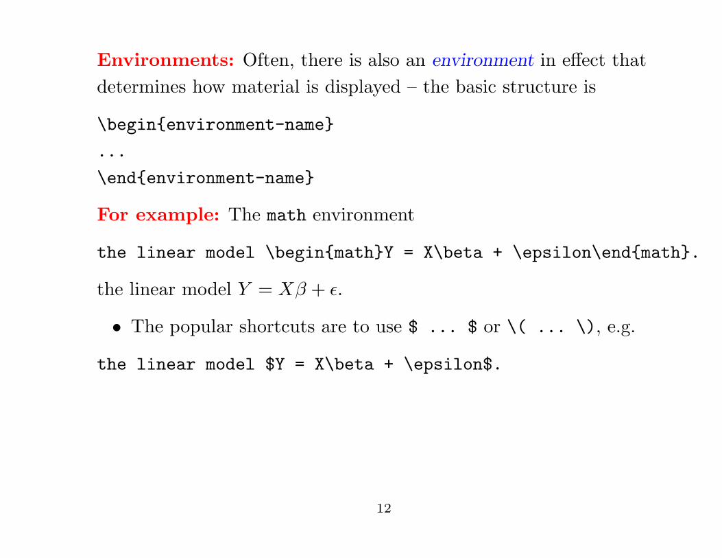
Environments: Often, there is also an environment in effect that

determines how material is displayed – the basic structure is

\beginenvironment-name

...

\endenvironment-name

For example: The math environment

the linear model \beginmathY = X\beta + \epsilon\endmath.

the linear model Y = Xβ + ǫ.

• The popular shortcuts are to use $ ... $ or \( ... \), e.g.

the linear model $Y = X\beta + \epsilon$.

12

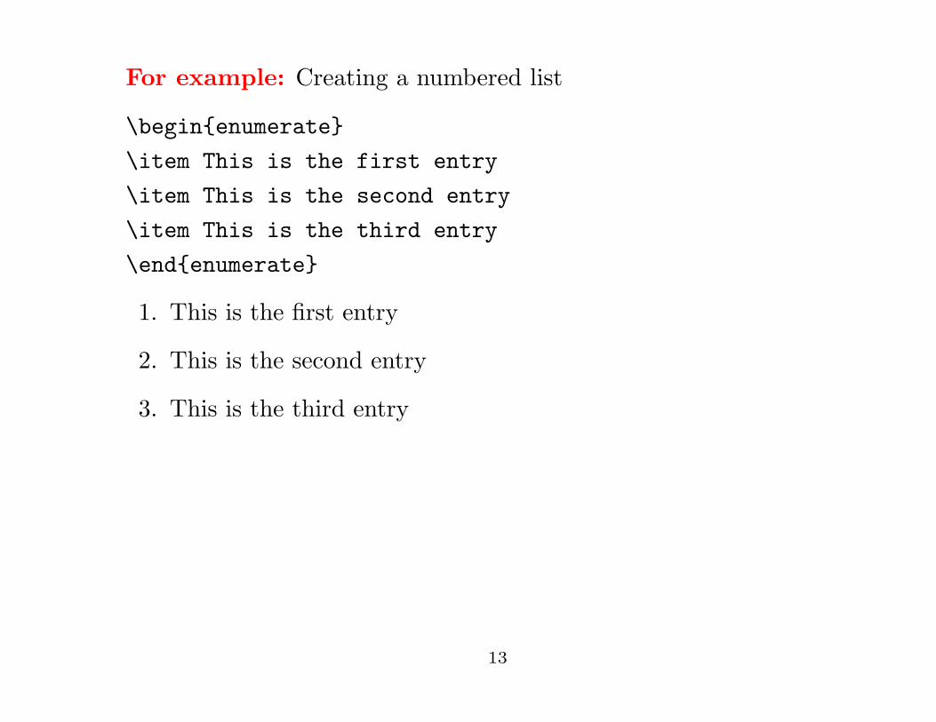
For example: Creating a numbered list

\beginenumerate

\item This is the first entry

\item This is the second entry

\item This is the third entry

\endenumerate

1. This is the first entry

2. This is the second entry

3. This is the third entry

13

Some popular environments:

Environment Mode Description

math math in-text mathematical expressions

displaymath math displayed mathematical expressions

equation math displayed expressions w/ line number

eqnarray math lines up equal signs, line numbers

eqnarray* math lines up equal signs, no line numbers

array math matrices and arrays

itemize paragraph list with bullets

enumerate paragraph list with numbers

description paragraph list with indentation

tabular LR align text in columns

table paragraph number and position table

figure paragraph number and position figure

center paragraph center text

mbox LR write text while in math mode

14

Math: LATEX is tailor-made for writing involving high mathematical

content! And it’s easy!

• Subscripts, superscripts, roots

e^y, x_ij, \sqrtx+y, \sum^n_i=1

ey, xij ,√

x + y,∑n

i=1

• Greek

\alpha,\beta,\gamma,\delta,\epsilon,\eta,\theta,\lambda

α, β, γ, δ, ǫ, η, θ, λ

\Gamma,\Delta,\Theta,\Lambda,\Omega,\Sigma

Γ, ∆, Θ, Λ, Ω, Σ

• Roofs

\hat\alpha,\tilde\alpha,\dotx,\overlinex,\barx

α, α, x, x, x

15

Math, continued:

• Binary operations

\pm,\times,\div,\cup,\otimes

±,×,÷,∪,⊗

• Relation symbols

\leq,\subset,\in,\geq,\equiv,\sim,\approx,\neq,\perp

≤,⊂,∈,≥,≡,∼,≈, 6=,⊥

• Arrows

\rightarrow,\Leftarrow,\Leftrightarrow,\uparrow

→,⇐,⇔, ↑

• Miscellaneous

\forall,\exists,\Re,\sum,\prod,\int

∀,∃,ℜ,∑

,∏

,∫

16

Math, continued: textstyle vs. displaystyle

• Math displayed as equations may be carried out using the

displaymath, equation, eqnarray*, eqnarray environments

• Shortcuts when equations are not numbered: $$ ... $$ or

\[ ... \]; e.g.,

$$\sum^n_i=1 x_i^2 (Y_ij-z_i \beta)$$

n∑

i=1

x2

i (Yij − ziβ)

• Some symbols appear differently depending on whether they are

in the text or displayed; e.g.,

$\sum^n_i=1$ VS. $$\sum^n_i=1$$

∑n

i=1VS.

n∑

i=1

• Can be overridden with textstyle and \displaystyle

17

Math, continued:

• Products, integrals, unions

$$\prod^n_j=1,\hspace0.1in \int^\infty_t f(u) du,

\hspace0.1in\bigcup_A: A \in \Omega$$n∏

j=1

,

∫ ∞

t

f(u)du,⋃

A:A∈Ω

• Special functions

$\exp(x), \log y, \sin(k\pi), \min_x f(x)$

exp(x), log y, sin(kπ), minx f(x)

• Fractions, partial derivatives

$$\frac\exp(x^T \beta)1+\exp(x^T \beta),

\frac\partial u\partial x$$

exp(xT β)

1 + exp(xT β),∂u

∂x

Note: Use \displaystyle for fractions; otherwise they are too small

18

Math, continued: There are different ways to present math in

boldface; here are two

• $\mbox\boldmath $X$$, $\mbox\boldmath $\Sigma$$

X, Σ

• $\mathbfX$, $\mathbf\Sigma$

X, Σ

19

Math, continued: array and eqnarray environments

• (2 × 3) matrix:

\left( \beginarrayccc

x_11 & x_12 & x_13\\

x_21 & x_22 & x_23 \endarray \right)

x11 x12 x13

x21 x22 x23

• Determinant of (2 × 2) matrix:

\left| \beginarraycc

a_11 & a_12 \\

a_21 & a_22 \endarray \right|∣∣∣∣∣∣

a11 a12

a21 a22

∣∣∣∣∣∣

20

Math, continued: array and eqnarray environments

• Braces

x = \left\ \beginarrayl \sin x \mbox if y<3, \\

\cos x \mbox if y \geq 3 \endarray \right.

x =

sinx if y < 3,

cos x if y ≥ 3

• Binomial coefficients:

\left( \beginarraycN \\ y \endarray \right)

N

y

21

Math, continued: array and eqnarray environments

• Equation with several lines, = signs lined up

\begineqnarray*

\Delta_i & = & \sum_j \sum_k \neq j \mboxCorr(Y_ij,Y_ik)

& = & \sum_j \sum_k \neq j \rho_i^\parallel j-k \parallel \\

& = & \frac2 \rho_i1-\rho_i \left\ n_i-1 -

\frac\rho_i(1-\rho_i^n_i-1)1-\rho_i \right\

\endeqnarray*

∆i =∑

j

∑

k 6=j

Corr(Yij , Yik)

=∑

j

∑

k 6=j

ρ‖j−k‖i

=2ρi

1 − ρi

ni − 1 − ρi(1 − ρni−1

i )

1 − ρi

22

The tabular environment:

• As with array, separate elements with &, make new line with \\

• Specify number of columns and type of justification at top, add

vertical and horizontal lines

\begintabularc|rr

& \multicolumn2cResults \\

Parameter & \multicolumn1cBias & \multicolumn1cSE \\

\hline

$\beta_0$ & $-$0.030 & 0.12 \\

$\beta_1$ & 0.002 & 0.07

\endtabular

Results

Parameter Bias SE

β0 −0.030 0.12

β1 0.002 0.07

23

NEWCOMMANDS

Motivation: In technical typing, the same (nasty) expression may

appear frequently

• A newcommand is like a “shortcut” to produce the expression

easily

• \newcommandkeywordtext

• A newcommand declaration may appear anywhere in a LATEX

source file (preamble or body) and is defined thereafter

• A newcommand keyword may not contain numbers

24

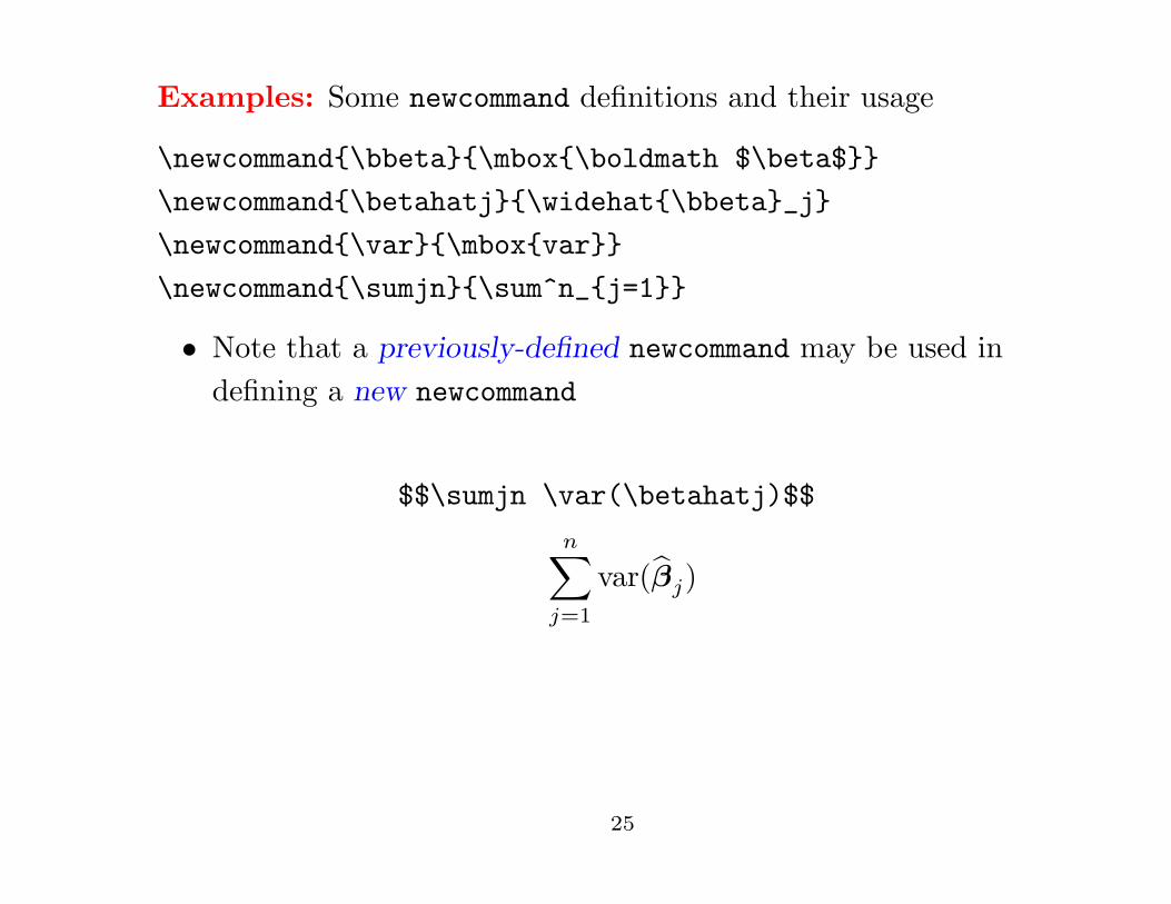
Examples: Some newcommand definitions and their usage

\newcommand\bbeta\mbox\boldmath $\beta$

\newcommand\betahatj\widehat\bbeta_j

\newcommand\var\mboxvar

\newcommand\sumjn\sum^n_j=1

• Note that a previously-defined newcommand may be used in

defining a new newcommand

$$\sumjn \var(\betahatj)$$

n∑

j=1

var(βj)

25

CROSS REFERENCES

Advantage: A built-in feature of LATEX is that it automatically

keeps track of sections, numbered equations, pages, and so on

• Sections, equations, tables, figures, pages etc. may be labeled

and referred to by the label

• If new labeled entities are added, LATEX renumbers them

automatically

• It is even possible to generate a table of contents and index for a

document

• To set up cross references correctly, must process a document

twice

LaTeX Warning: Label(s) may have changed. Rerun to get cross-references right.

26

Examples:

• Numbered equation

\beginequation

\var(\alpha) = \sumjn \var(\betahatj)

\labeleq:alpha

\endequation

In equation~\refeq:alpha, we see that...

27

Examples, continued:

• Section label

\sectionIntroduction

\labels:intro

...As discussed in Section~\refs:intro, kurtosis...

• Page label

Thus, we see that calculation of the variance is

straightforward \labelp:var

...On page~\pagerefp:var, the variance calculation...

28

PACKAGES

Useful utilities: LATEX is much more powerful than the intrinsic

features would suggest

• A huge user community

• Contributed document classes, “add-ons” to allow different

capabilities and customization

• “Packages”

• Define new commands, syntax, etc.

• Visit CTAN (see slide 50)

29

Example: shadow.sty – make “shadowboxes”

• In preamble

\usepackageshadow

\shaboxThis stuff

This stuff

In addition: There are also user-defined, alternative document

classes

• Journals, book publishers may have their own class to create

articles, pages with a specific format

30

Dissertations: At NCSU, dissertations may be created in LATEX

using special a special style; to learn more, visit

http://www2.acs.ncsu.edu/grad/ETD/tutorial/latex.htm

http://www.stat.ncsu.edu/computing/howto/latex/session_2/session2.html

31

IMPORTING GRAPHICS

Numerous options: We discuss three of these

• psfig – \usepackagepsfig

\psfigfigure=dental.ps,height=2.5in

32

age (years)

dist

ance

(m

m)

8 9 10 11 12 13 14

2025

30

0 0 0

0

0

0

0

0

0

0

0

1

1

1

1

1

1

1

1

1

1

1

1

1

11

1

0

0

0 0

0

0

0 0

0

0

01

11

1

1

1

11

1

1

11

1

1

1

1 0

0 0 0

0

0

0 0

0

0

0

1

1

1

1

1

1

11

11

11

111

1 0

0 0 0

0

0

0

0

0

0

0

1

1

11

1

1

1

11

1

1

1

1

1

1

1

Dental Study Data

33

• epsf – \usepackageepsf

\epsfysize=2.5in

\epsfboxdental.ps

34

age (years)

dist

ance

(m

m)

8 9 10 11 12 13 14

2025

30

0 0 0

0

0

0

0

0

0

0

0

1

1

1

1

1

1

1

1

1

1

1

1

1

11

1

0

0

0 0

0

0

0 0

0

0

01

11

1

1

1

11

1

1

11

1

1

1

1 0

0 0 0

0

0

0 0

0

0

0

1

1

1

1

1

1

11

11

11

111

1 0

0 0 0

0

0

0

0

0

0

0

1

1

11

1

1

1

11

1

1

1

1

1

1

1

Dental Study Data

35

• graphicx – \usepackagegraphicx

• Can also import other formats (pdf, jpg, etc)

\includegraphics[height=2.5in]dental.ps

36

age (years)

dist

ance

(m

m)

8 9 10 11 12 13 14

2025

30

0 0 0

0

0

0

0

0

0

0

0

1

1

1

1

1

1

1

1

1

1

1

1

1

11

1

0

0

0 0

0

0

0 0

0

0

01

11

1

1

1

11

1

1

11

1

1

1

1 0

0 0 0

0

0

0 0

0

0

0

1

1

1

1

1

1

11

11

11

111

1 0

0 0 0

0

0

0

0

0

0

0

1

1

11

1

1

1

11

1

1

1

1

1

1

1

Dental Study Data

37

TABLES AND FIGURES

Two standard LATEX environments: table and figure

• Automatically numbers tables and figures

• Allow tables and figures to be formatted and referenced within a

document

• Allow captions

38

\begintable

\begincenter

\begintabularc|rr

& \multicolumn2cResults \\

Parameter & \multicolumn1cBias & \multicolumn1cSE \\

\hline

$\beta_0$ & 0.030 & 0.12 \\

$\beta_1$ & 0.002 & 0.07

\endtabular

\endcenter

\caption\it Results of the simulation>

\labelt:simresults

\endtable

39

Results

Parameter Bias SE

β0 0.030 0.12

β1 0.002 0.07

Table 1: Results of the simulation.

• Reference – In Table~\reft:simresults, we see that...

• In Table 1, we see that. . .

40

\beginfigure

\caption\it The dental data of Pothoff and Roy.

\labelf:dental

\begincenter

\includegraphics[height=2.5in]dental.ps

\endcenter

\endfigure

41

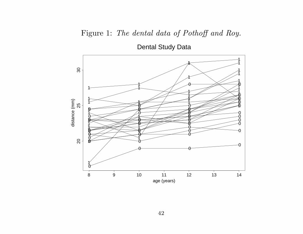
Figure 1: The dental data of Pothoff and Roy.

age (years)

dist

ance

(m

m)

8 9 10 11 12 13 14

2025

30

0 0 0

0

0

0

0

0

0

0

0

1

1

1

1

1

1

1

1

1

1

1

1

1

11

1

0

0

0 0

0

0

0 0

0

0

01

11

1

1

1

11

1

1

11

1

1

1

1 0

0 0 0

0

0

0 0

0

0

0

1

1

1

1

1

1

11

11

11

111

1 0

0 0 0

0

0

0

0

0

0

0

1

1

11

1

1

1

11

1

1

1

1

1

1

1

Dental Study Data

42

Useful package: subfigure – \usepackagesubfigure

• Create a “multipanel” figure from several files with each panel

labeled

\beginfigure

\centering \subfigure[]

\includegraphics[width=1.5in]dental.ps

\hspace*0.1in

\subfigure[]

\includegraphics[width=1.5in]dental.ps

\caption(a) The dental data of Pothoff and Roy. (b) The dental

data of Pothoff and Roy, again.

\labelf:dental2

\endfigure

43

age (years)

dist

ance

(m

m)

8 9 10 11 12 13 14

2025

30

0 0 0

0

0

0

0

0

0

0

0

1

1

1

1

1

1

1

1

1

1

1

1

1

11

1

0

0

0 0

0

0

0 0

0

0

01

11

1

1

1

11

1

1

11

1

1

1

1 0

0 0 0

0

0

0 0

0

0

0

1

1

1

1

1

1

11

11

11

111

1 0

0 0 0

0

0

0

0

0

0

0

1

1

11

1

1

1

11

1

1

1

1

1

1

1

Dental Study Data

(a)

age (years)

dist

ance

(m

m)

8 9 10 11 12 13 14

2025

30

0 0 0

0

0

0

0

0

0

0

0

1

1

1

1

1

1

1

1

1

1

1

1

1

11

1

0

0

0 0

0

0

0 0

0

0

01

11

1

1

1

11

1

1

11

1

1

1

1 0

0 0 0

0

0

0 0

0

0

0

1

1

1

1

1

1

11

11

11

111

1 0

0 0 0

0

0

0

0

0

0

0

1

1

11

1

1

1

11

1

1

1

1

1

1

1

Dental Study Data

(b)

Figure 2: (a) The dental data of Pothoff and Roy. (b) The dental data

of Pothoff and Roy, again.

44

PICTURES

LATEX can “draw”:

• picture environment

• The following is a simple picture – circles, curves, ovals, etc are

also possible (see the documentation)

45

Two-compartment open model with IV administration:

C(t)

-k12

k21

Ctis(t)D :

?

ke

dC(t)

dt= k21Ctis(t) − k12C(t) − keC(t),

Ctis(t)

dt= k12C(t) − k21Ctis(t), Ctis(0) = 0

46

Picture was made with:

\setlength\unitlength1in

\beginpicture(5,1)

\put(0.5,0.5)\framebox(1.5,1)$C(t)$

\put(2,1.25)\vector(1,0)0.5

\put(2.25,1.35)\makebox(0,0)$k_12$

\put(2.5,0.75)\vector(-1,0)0.5

\put(2.25,0.85)\makebox(0,0)$k_21$

\put(2.5,0.5)\framebox(1.5,1)$C_tis(t)$

\put(0.25,1)\makebox(0,0)$D:$

\put(1.25,0.5)\vector(0,-1)0.3

\put(1.35,0.35)\makebox(0,0)$k_e$

\endpicture

\endcenter

47

Other “drawing” resources:

• The pstricks package – really intricate stuff like grids, plots of

functions, etc (see class web page for link to documentation)

• xfig

48

WHERE TO LEARN MORE

Books and guides:

• Lamport, L. (1994) LATEX: A Documentation Preparation

System, User’s Guide and Reference Manual (The creator of

LATEX)

• Goossens, M. et al. (1994) The LATEX Companion

• Kopka, H. (1999) A Guide to LATEX : Document Preparation for

Beginners & Advanced Users

• Hahn, J. (1993) LATEX for Everyone: A Reference Guide and

Tutorial for Typesetting Documents Using a Computer

• Oetiker, T. et al. (2002) The Not So Short Introduction to

LATEX 2ε (Available on the class web page)

49

Resources online and on the Web:

• The Comprehensive TEX Archive Network (CTAN)

http://www.ctan.org – a repository of tons of style files,

packages, etc.

• Several free guides available on unity at

/afs/bp.ncsu.edu/contrib/tetex107/share/texmf/doc/latex/general

(as .dvi or .ps files)

• Local intro tutorial

http://www.stat.ncsu.edu/computing/howto/latex/session 1/

50