Embed Size (px)
Citation preview
Research ArticleA Hybrid Simulated Annealing Heuristic for MultistageHeterogeneous Fleet Scheduling with Fleet Sizing Decisions
Bing Li Xinyu Yang and Hua Xuan
School of Management Engineering Zhengzhou University Zhengzhou 450001 Henan China
Correspondence should be addressed to Bing Li lbingzzueducn
Received 22 September 2018 Revised 19 December 2018 Accepted 20 December 2018 Published 10 January 2019
Academic Editor Giulio E Cantarella
Copyright copy 2019 Bing Li et al This is an open access article distributed under the Creative Commons Attribution License whichpermits unrestricted use distribution and reproduction in any medium provided the original work is properly cited
This paper deals withmultistage heterogeneous fleet scheduling with fleet sizing decisions (MHFS-FSD)ThisMHFS-FSD attemptsto integrate vehicles allocation and fleet sizing decisions considering the vehicle routing of multiple vehicle types The problem isformulated asmixed integer programmingmodelThematrix formulation denoting vehicle allocation scheme is explored accordingto the characteristic of this problem Generating vehicle allocation scheme with greedy heuristic procedure (VA-GHP) as initialsolution of problem is presentedThe USP-IVAmethod to update the initial solution generated by VA-GHP approach is developedAnd then incorporating VA-GHP and USP-IVA into simulated annealing algorithm a novel heuristic called HSAH-GHPampIVA isproposed Finally some experiments are designed to test the proposed heuristic and the results show that the heuristic can generatereasonably good solutions in short CPU times
1 Introduction
Freight transport companies frequently face the problem ofmanaging a fleet of vehicles which circulate on networksbeing dispatched loaded or repositioned empty betweenvarious freight terminals of the networkThere is recognitionof the importance of managing fleets in trucking industryrailroad industry and shipping industry
Prior research has most commonly focused on a homo-geneous fleet of vehicles But due to the large amountof loads and complex transport routing conditions manyconflicts will arise between homogeneous fleet of vehiclesand heterogeneity transport demands when freight transportschemes are carried out Instead of homogeneous fleet withsubstitution of single vehicle types for different types of trans-port demands setting up heterogeneous fleets of vehiclesis an effective strategy to enhance the efficiency of vehicleutilisation
In addition the fleet size decisions are significant toimprove the freight carry capacity of fleet The insufficientvehicles and oversize vehicles can be ineffective in supportingfleet management
The study on heterogeneous fleet of various vehicle typeswith fleet sizing decisions is regarded as a promising per-spective for the improvement of freight transport schedulingsystems The combinatorial nature of the problem causes themodel formulated to be very hard to solve Therefore theresearch focuses on the development of powerful methodsthat are able to obtain solutions in reasonable time
In this paper we focus on scheduling a heterogeneousfleet of various vehicles over time to serve a set of loadswith fleet sizing decisions considering the vehicle routingof multiple vehicle types We name this type of problem asmultistage heterogeneous fleet scheduling with fleet sizingdecisions (MHFS-FSD) The objective is to maximise totalprofits over the entire planning horizon We develop a mixedinteger programming model and present a novel hybridsimulated annealing heuristic called HSAH-GHPampIVA
The remainder of this paper is organised as followsSection 2 of this paper discusses related earlier researchefforts Section 3 is devoted to the mathematical descriptionof the MHFS-FSD In Section 4 we describe the math-ematical formulation Section 5 explains the approach ofgenerating vehicle allocation scheme with greedy heuristic
HindawiJournal of Advanced TransportationVolume 2019 Article ID 5364201 19 pageshttpsdoiorg10115520195364201
2 Journal of Advanced Transportation
procedure (VA-GHP) as initial solution of problem Wedevelop the updating solution procedure by improving vehi-cle allocation (USP-IVA) in Section 6 And then the hybridsimulated annealing heuristic called HSAH-GHPampIVA isproposed in Section 7 The computational experiments aredescribed in Section 8 and the effectiveness of the proposedmethod is shown from the computational results The lastsection concludes with a summary of current work andextensions
2 Literature Review
21 State of the Article In this section we review the relevantliterature about fleet scheduling problems Literature reviewindicates that fleet scheduling problems can be dividedinto four groups that is vehicle routing problem vehicleassignment transportation network optimisation and fleetmanagement
In recent years many researches on vehicle routingproblem have been carried out The inventory routing prob-lems with pickups and deliveries (IRP-PD) is studied byArchetti et al [1] with a branch-and-cut method Cian-cio et al [2] transformed the Mixed Capacitated GeneralRouting Problem with Time Windows (MCGRPTW) intoan equivalent node routing problem over a directed graphand solved the equivalent problem by using a branch-price-and-cut algorithm A new combinatorial algorithm namedOVRP GELS based on gravitational emulation local searchalgorithm was obtained to solve the open vehicle routingproblem (OVRP) by Hosseinabadi et al [3] The Pickup andDelivery Traveling Salesman Problem with Multiple Stackswas researched by Sampaio and Urrutia [4] They provideda new integer programming formulation with a polyhedralrepresentation and a branch-and-cut algorithm for solvingthe proposed formulation A two-phase approach to dealwith the vehicle routing problems with backhauls and timewindows is introduced by Reil et al [5] They proposed Tabusearch and first amultistart evolutionary strategy tominimisethe total travel distance Archetti et al [6] designed andimplemented a multistart heuristic which produces solutionswith small errors when compared with optimal solutionsobtained by solving an integer programming formulationwith a commercial solver Andelmin and Bartolini [7] pre-sented an exact algorithm for solving the green vehiclerouting problem andmodeled theG-VRP as a set partitioningproblem
The proper configuration of the vehicle assignment isthe crucial point of the research on the optimisation offleet resource allocation Choi et al [8] proposed a Dantzig-Wolfe decomposition approach for the vehicle assignmentproblemwith demanduncertainty in a hybrid hub-and-spokenetwork Spliet et al [9] developed a branch-price-and-cutalgorithm to arrange the time windows for time windowassignment vehicle routing problems with the objective ofminimising the expected transportation costs Lin et al [10]addressed dynamic vehicle allocation problem Taking thewaiting cost of transportation operation as the objective func-tion of the problem a Markov decision model is constructedand applied to the automated material handling system in
semiconductor manufacturing Joao et al [11] presented aflight scheduling and fleet assignment optimisation modelthat may assist public authorities to establish the level ofservice requirements for subsidized air transport networksSargut et al [12] introduced a multiobjective integrated crewrostering and vehicle assignment problem and developeda new multiobjective Tabu search algorithm Li and Xuan[13] provided a greedy algorithm for solving the vehicleassignment with time window restraints
The optimisation of transportation network plays a vitalrole in improving fleet income and reducing various costsThe urban rail transit systems are optimised by Ozturk andPatrick [14]They extended the setting to several stations anddeveloped a heuristic method two mixed integer modelsand a constraint after proposing an approximation algorithmand a pseudopolynomial dynamic programming algorithmbetween two sites Zhang and Zhang [15] explored thedynamic shortest path from a single source to a destinationin a given traffic network To optimise the journey timefor the traveler a novel dynamic shortest path algorithmbased on hybridizing genetic and ant colony algorithms wasdeveloped A feasible flow-based iterative algorithm namedTHTMTP-A is presented to deal with the two-level hierar-chical time minimisation transportation problem by Xie etal [16] Suhng and Lee [17] developed a new Link-BasedSingle Tree Building Algorithm in order to reduce the slowexecution speed problem of the multitree building algorithmfor shortest path searching in an Urban Road Transporta-tion Network and proved its usefulness by comparing theproposed one with other algorithms The suitability of threedifferent global optimisation methods which included thebranch and reduce method the branch and cut methodand the combination of global and local search strategiesfor specifically the exact optimum solution of the nonlineartransportation problem is studied by Klansek and Psunder[18]
The fleet management is one of themost important as it isa major fixed investment for starting any business Hashemiand Sattarvand [19] studied the different management sys-tems of the open pit mining equipment including nondis-patching dispatching and blending solutions for the Sunguncoppermine A dispatching simulationmodel with the objec-tive function of minimising truck waiting times had beendeveloped Zhu et al [20] focused on solving the scheduledservice network design problem for freight rail transportationand proposed a heuristic solution methodology integratingslope scaling a dynamic block-generation mechanism long-term-memory-based perturbation strategies and ellipsoidalsearch Li et al [21 22] respectively developed an alternatingsolution strategy for the stochastic dynamic fleet schedulingproblem with variable period and presented a piecewisemethod by updating preset control parameters for dynamicworking vehicle scheduling problem Tierney et al [23]studied a central problem in the liner shipping industry calledthe liner shipping fleet repositioning problem and introduceda simulated annealing algorithm for above problem Hugoet al [24] designed an approximate dynamic programmingalgorithm for large-scale fleet management
Journal of Advanced Transportation 3
22 Contributions Overall the objectives of this researchare twofold The first objective is to develop a mathematicalmodel of MHFS-FSD In the proposed model the matrixformulation denoting vehicle allocation scheme is exploredaccording to the characteristic of this problem The secondobjective is to propose an efficient methodology for solvingthe model Specifically the contributions of this paper are asfollows
(1) We develop the mixed integer programming model(MIP) This model discusses the integration of vehi-cles allocation and fleet sizing decisions consideringthe vehicle routing of multiple vehicle types Par-ticular vehicle type is assigned to some particulartransport routing according to the classification ofvehicles The matching of vehicle type and transportroute is given According to the characteristic of thisproblem the matrix formulation denoting vehicleallocation scheme is provided
(2) According to the specific structure of the mixedinteger programming model the approach of gener-ating vehicle allocation scheme with greedy heuristicprocedure (VA-GHP) as initial solution of problemis presented On the basis of the initial solution gen-erated by VA-GHP approach the USP-IVA methodto update the initial solution is developed and thenincorporating VA-GHP and USP-IVA into simulatedannealing algorithm a novel heuristic called HSAH-GHPampIVA is proposed
(3) To evaluate the performance of the heuristics pro-posed we generated randomly three sets of probleminstances with different size of freight terminal andtime periods considering different number of vehi-cles types Three sets of experiments are oriented toevaluate the performances of the hybrid simulatedannealing heuristic The results show that the pro-posed heuristic is able to obtain reasonably goodsolutions in short CPU times
3 Problem Description and Analysis
This section describes the problem of scheduling a heteroge-neous fleet of various vehicles over time to serve a set of loadswith fleet sizing decisions We make a brief overview of somefoundational concepts and analysis of the problem
31 Problem Description The freight transportation schedul-ing frequently aims to obtain appropriate capacity of trans-portation systems discover the potential of fleets of vehicleswhich circulate on networks and improve transportationefficiency by arranging daily transportation production rea-sonably organising vehicles flow adjustment scientificallyand making plans for loading and unloading operations intheir destination terminal of the networks efficiently
This paper discusses the integration of vehicles allocationand fleet sizing decisions considering the vehicle routingof multiple vehicle types Let 119866(119873 119864) represent the freighttransport network where 119873 is a set of freight terminal and
E represents the set of the movement of vehicles betweena pair of freight terminal We assume that time is dividedinto a set of discrete time periods 119867 = ℎ | ℎ = 1 119870where K is the length of the planning horizon and ℎ is thetime period All transitions require multiperiod travel timesLet 119905119894119895 be the travel time from 119894 to 119895 119894 119895 isin 119873 The traveltime between any pair of terminals is different length of timeperiod and integermultiple of one time periodThe operatorsof transportation systems manage a heterogeneous fleet ofvarious vehicles We define the set of classification of vehiclesas119882 = 1 sdot sdot sdot 119875 Particular vehicle type is assigned to someparticular vehicle routing according to the classification ofvehicles The matching of vehicle type and vehicle routingis given The use of operation vehicles will generate fixedexpenses such as vehicle leasing and daily maintenanceIt is crucial to decide the size of various vehicle typesreasonably
To maximise total profits over a given horizon theproblem is to optimise the fleet sizing and make the vehicleutilisation decision in view of the profit derived frommovinga load from terminal 119894 to terminal j denoted as 120572119908119894119895 the costof moving an empty vehicle from terminal 119894 to terminal 119895denoted as 120573119908119894119895 the fixed costs of owning or leasing a type ofvehicles denoted as 120574119908 and vehicle routing of vehicle typesdenoted as 120587119908 Figure 1 displays a snapshot of dynamic space-time network for fleet scheduling with multiperiod traveltimes
32 Understanding Vehicle Allocation between Pairs of Ter-minals A fleet of vehicles must be assigned to loads thathave the effect of moving the vehicle from one terminal tothe next The operator of the fleet must either assign eachvehicle to a requested loaded movement or move it empty toanother terminal to pick up a requested loadedmovement orto hold it in the same terminal until the next time period Sothe allocation problem of loaded vehicle and empty vehiclearises
Serving loads results in the relocation of vehiclesDemands request a vehicle to be available in a specificterminal on a specific time period to carry the load to a givendestination terminal Each load must be served by a vehicleLoaded movement will generate revenue So the loadedvehicle assignment is the basis of the vehicle allocation
The load for movements between various terminals isoften imbalanced and this implies the need for redistributionof empty vehicles over the transport network from terminalsat which they have become idle to terminals at which they canbe reused It is important to manage empty vehicle flows intransport network The loads create requirements for emptyvehicleThe arrivals of loaded vehicle flow create the suppliesof empties available for repositioning
Vehicle allocation has significant effects on the vehicledistribution or utilisation decision and then effects on capac-ity and efficiency of transport network
33 Understanding Heterogeneous Fleet of Vehicles Due tothe huge transport networks the large amount of loads andcomplex transport route conditions many conflicts will arisebetween homogeneous fleet of vehicles and heterogeneity
4 Journal of Advanced Transportation
Time periodKh h+1 h+2
Freight terminal 1
1
Freight terminal i
Freight terminal j
Freight terminal k
Freight terminal A
ℎ
Figure 1 Dynamic space-time network for fleet scheduling with multiperiod travel times
transport demands when freight transport schemes are car-ried out A homogeneous fleet with single vehicle type meansinefficiency in satisfying the diverse transport demandWhenthe operators manage a homogeneous fleet the vehicle short-age and idleness may occur synchronously The worseningtrend of vehicle utilisation is also possible to appear sothat transport efficiency is reduced and transport cost isenhanced Instead of homogeneous fleet with substitution ofsingle vehicle types for different types of transport demandssetting up heterogeneous fleets of vehicles is an effectivestrategy to eliminate the above unreasonable phenomenaoptimise the vehicle allocation and enhance the efficiency ofvehicle utilisation
Meanwhile the fleet size decisions are significant toimprove the freight carry capacity of fleet The insufficientvehicles seriously affect the implementation of transportwork If the number of available vehicles is not enough tomeet transport demand the penalty cost for unmet demandwill generate On the other hand the oversized supply of fleetfar more than the transport demand causes a large number ofvehicles to be idle
34 Understanding Vehicle Routing for Particular VehicleTypes Many works have assumed a homogeneous fleetof vehicles But most problems in practice have multiplevehicle types with limited substitution In this paper weextend the methodology to handle heterogeneous fleets ofvehicles with different vehicle types for different transportrouting
The two stage freight transport network is comprised offreight supply location as origin terminal and freight demandlocation as destination terminal In practical considerationsthe route from any supply location to demand locationcannot always be used to carry freight due to limited vehicletypes transport routing condition transport routing external
1
3
4
6
2A
5
1
3
4
6
2A
5
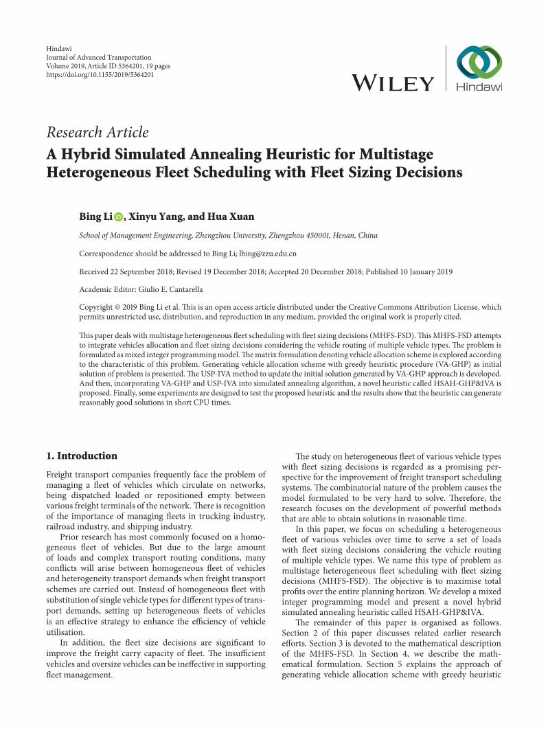
Figure 2 The vehicle routing of multiple vehicle types
environment and so on The specific reasons can be diverseas follows
(1) Some transport routes cannot be used by some specificvehicle type due to carry capacity of the road
(2) Some specific vehicle types are not allowed to travelon certain transport routes due to physical condition of theroad versus maintenance condition of vehicles
(3) Due to inexistence of supply location and demandlocation for freight exchange some transport routes disap-pear
An illustration of the vehicle routing of multiple vehicletypes is shown in Figure 2
Because some specific vehicle types are only allowed totravel on certain transport routes we use 120587 as the matchingmatrix such that 120587119908119894119895 = 1 if 119908 types of vehicle can be assignedto movement from terminal 119894 to 119895 and 120587119908119894119895 = 0 otherwise Wepresent the notation formore clearly expressing thematchingmatrix here119873 is the set of freight terminal in the freight transportnetwork Define 119873 = 1 sdot sdot sdot 119860 where A is the number offreight terminal119882 is the set of vehicle types in the heterogeneous fleetDefine 119882 = 1 sdot sdot sdot 119875 where 119875 is the total number ofavailable vehicles of various types
Journal of Advanced Transportation 5
119879 is thematrix of travel time of vehicles set between a pairof freight terminal We have
119879 =[[[[[[[[[[[[
0 sdot sdot sdot 1199051119895 sdot sdot sdot 1199051119860 1199051198941 sdot sdot sdot 119905119894119895 sdot sdot sdot 119905119894119860 1199051198601 sdot sdot sdot 119905119860119895 sdot sdot sdot 0
]]]]]]]]]]]]
forall119894 119895 isin 119873 (1)
120587 is the matrix of vehicle routing for certain vehicle typeThe matrix can be expressed by 120587 = 120587119908 | 119908 = 1 sdot sdot sdot 119875 Theparameter 120587119908 is used to represent practical situations wherevehicle type 119908 can be allowed to transport load on certainroutes Correspondingly we denote that
120587119908 =[[[[[[[[[[[[
12058711990811 sdot sdot sdot 1205871199081119895 sdot sdot sdot 1205871199081119860 1205871199081198941 sdot sdot sdot 120587119908119894119895 sdot sdot sdot 120587119908119894119860 1205871199081198601 sdot sdot sdot 120587119908119860119895 sdot sdot sdot 120587119908119860119860
]]]]]]]]]]]]
120587119908119894119895=
0 if vehicle type 119908 can move from terminal 119894 to 1198951 otherwise
forall119894 119895 isin 119873 119908 isin 119882
(2)
4 Mathematical Formulation
In this section we define the notation and formulate mul-tistage heterogeneous fleet scheduling with fleet sizing deci-sions (MHFS-FSD) as a mixed integer programming model
In the following we describe the model parameters andvariables used to model the MHFS-FSD
41 Model Parameters The parameters are needed todescribe the problem119905119894119895 is the travel time moving from origin 119894 to destination 119895and is the integer multiple of the scheduling time period120587119908119894119895 is the parameter for representing whether or notvehicle type119908 can be allowed to carry freight along transportrouting (119894 119895) The value of 120587119908119894119895 is 1 if the 119908 types of vehicle cancarry freight from the terminal 119894 to the terminal 119895 otherwisethe value is 0 forall119908 isin 119882 and forall119894 119895 isin 119873119902ℎ119894119895 is the set of loads with origin 119894 and destination 119895 havingℎ as a feasible departure forallℎ isin 119867 forall119894 119895 isin 119873120572119894119895 is the profits generated by a unit load being dispatchedfrom terminal 119894 to terminal 119895 forall119908 isin 119882 forall119894 119895 isin 119873120573119908119894119895 is the cost of 119908 type vehicle being repositioned emptyfrom terminal 119894 to terminal 119895 forall119908 isin 119882 forall119894 119895 isin 119873120574119908 is the purchase or lease cost for the 119908 type of vehicleforall119908 isin 119882120582119908 is the loading capacity of119908 type vehicle forall119908 isin 119882 Thatis to say it is the amount of loads which can be serviced byone 119908 type vehicle119911119908119894119905 is the number of available vehicle of119908 type at terminal119894 in time period t forall119908 isin 119882 forall119894 isin 119873
42Model Variables Thedecision variables of themathemat-ical model are119909ℎ119908119894119895 is the number of 119908 type of loaded vehicles fromterminal 119894 to terminal 119895 at time period ℎ forall119894 119895 isin 119873 ℎ isin 119867119910ℎ119908119894119895 is the number of 119908 type of empty vehicles fromterminal 119894 to terminal 119895 at time period ℎ forall119894 119895 isin 119873 ℎ isin 119867119911119908 is the number for available vehicle of 119908 type
43 Mathematical Models The mathematical models formultistage heterogeneous fleet scheduling with fleet sizingdecisions (MHFS-FSD) are given by
max 119865 (119909 119910 119911) = sum119908isin119882
( 119870sumℎ=1
sum119894isin119873
sum119895isin119873
(120572119894119895 sdotmin119902ℎ119894119895 sum119908isin119882
120582119908119909ℎ119908119894119895 minus 120573119908119894119895119909ℎ119908119894119895 minus 120573119908119894119895119910ℎ119908119894119895 ) minus 120574119908119911119908) (3)
119904119905 sum119895isin119873
(119909ℎ119908119894119895 + 119910ℎ119908119894119895 ) 120587119908119894119895 = 119911ℎ119908119894 forall119894 isin 119873 forallℎ isin 119867 forall119908 isin 119882 (4)
sum119908isin119882
120582119908119909ℎ119908119894119895 le 119902ℎ119894119895 forall119894 119895 isin 119873 forallℎ isin 119867 (5)
sum119894isin119873
(119909(ℎminus119905119894119895)119908119894119895 + 119910(ℎminus119905119894119895)119908119894119895 ) 120587119908119894119895 = 119911ℎ119908119895 forall119895 isin 119873 forallℎ isin 119867 forall119908 isin 119882 (6)
sum119894isin119873
119911ℎ119908119894 = 119911119908 forallℎ isin 119867 (7)
119909ℎ119908119894119895 ge 0 119910ℎ119908119894119895 ge 0 119911119908 ge 0 integer forall119894 119895 isin 119873 forallℎ isin 119867 forall119908 isin 119882 (8)
6 Journal of Advanced Transportation
The MHFS-FSD model belongs to a mixed integer pro-gramming model (MIP) The objective function (3) aims tomaximise the total profit generated by the fleet schedulingscheme during the whole planning horizon Constraint (4)denotes the number of dispatching loaded vehicles andempty vehicles are determined by supplies of vehicles in timeperiod Constraint (5) ensures that the number of loadedvehicle cannot exceed available requirements of all loads ineach terminal at each time period Constraint (6) denotesupdating equation for total supply of vehicle of various typesConstraint (7) shows having flow conservation of vehicle ineach type Finally constraint (8) defines the range of decisionvariables constraints
As an NP problem using traditional method for solvingMHFS-FSDmodel is difficult and inefficient A novel heuris-tic method is considered to solve this problem
5 Generating Initial Solution with VA-GHP
According to the characteristic of this problem the matrixformulation denoting vehicle allocation scheme is providedAnd then the approach of generating vehicle allocationscheme with greedy heuristic procedure as initial solution ofproblem is presented
51 Matrix Formulation of Vehicle Allocation The solution ofMHFS-FSD model represents the vehicle allocation schemeThe solution is expressed as two stage structureThe first termin the solution is matrix formulation of loaded vehicle dis-patching scheme The second term is the matrix formulationof empty vehicle reposition scheme
(1) e Matrix Formulation of Loaded Vehicle DispatchingScheme The first section of the solution is used to representthe loaded vehicle dispatching scheme of carrying freightfrom the origin terminal to the destination terminal Thissection is formulated as the matrix form which has 119860 rowsandA columns Each component in row and row intersectionof the matrix indicates the number of 119908 type loaded vehiclesfrom origin terminal to destination terminal The allocationscheme of loaded vehicle is written as the following formula
119909119908 =[[[[[[[[[[[[
11990911990811 sdot sdot sdot 1199091199081119895 sdot sdot sdot 1199091199081119860 1199091199081198941 sdot sdot sdot 119909119908119894119895 sdot sdot sdot 119909119908119894119860 1199091199081198601 sdot sdot sdot 119909119908119860119895 sdot sdot sdot 119909119908119860119860
]]]]]]]]]]]]
119908 isin 119882 (9)
(2) e Matrix Formulation of Empty Vehicle RepositionScheme The second section of the solution is used to denotethe empty vehicle reposition scheme of vehiclemoving emptyfrom the origin terminal to the destination terminal Thissection is also formulated as the matrix form which has119860 rows and 119860 columns Each component in row and rowintersection of the matrix expresses the number of 119908 typeempty vehicles from origin terminal to destination terminal
The allocation scheme of loaded vehicle is expressed as thefollowing formula
119910119908 =[[[[[[[[[[[[
11991011990811 sdot sdot sdot 1199101199081119895 sdot sdot sdot 1199101199081119860 1199101199081198941 sdot sdot sdot 119910119908119894119895 sdot sdot sdot 119910119908119894119860 1199101199081198601 sdot sdot sdot 119910119908119860119895 sdot sdot sdot 119910119908119860119860
]]]]]]]]]]]]
119908 isin 119882 (10)
52 Greedy Heuristic Procedure to Generate Vehicle AllocationScheme According to the fundamental principles of priori-tising to consider the vehicle types with large load capacityand transport routing with large carry capacity the greedyheuristic procedure is presented to generate vehicle allocationscheme We name this approach as vehicle allocation withgreedy heuristic procedure (VA-GHP) An overview of theframework of VA-GHP is explained as follows
Stage 1 (set of vehicle types selection sequence) Accordingto the vehicle distribution 119911ℎ119908119894 in terminal 119894 at ℎ time periodthe set of vehicle types selection sequence 119882ℎ119894 is obtainedwith ranking the vehicle types in descending order by loadingcapacity 120582119908 We denote 120575 as serial number of the vehicle typein this set and 120575 as the total quantity of available vehicle typesThus119882ℎ119894 has the form of
119882ℎ119894 = 119908ℎ119894 (120575) | 119908ℎ119894 (120575) = 119908 119908 isin 119882 120575 = 1 sdot sdot sdot 120575 (11)
Stage 2 (set of fleet size selection sequence) Let119885ℎ119894 be the setof fleet size selection sequence According to the set of vehicletypes selection sequence119882ℎ119894 we can express 119885ℎ119894 as
119885ℎ119894 = 119911ℎ119894 (120575) | 119911ℎ119894 (120575) = 119911ℎ119908119894 119908 isin 119882ℎ119894 120575 = 1 sdot sdot sdot 120575 (12)
Stage 3 (set of transport routing selection sequence) Werandomly choose the terminal 119894 from the set of freightterminal and compute the revenue 120572119894119895119902ℎ119894119895 created by loadedvehicle dispatched from origin 119894 to any available destination119895 We rank the transport routing in order of the revenuefrom high to low and the set of transport routing selectionsequence 119878ℎ119894 can be given We use 120585 to denote the serialnumber of transport routing in this set and the total numberof transport routing is represented as 120585ℎ119894 Here 119878ℎ119894 is written as
119878ℎ119894 = 119904ℎ119894 (120585) | 119904ℎ119894 (120585) = (119894 119895) 119895 isin 119873 120585 = 1 sdot sdot sdot 120585ℎ119894 (13)
The set of transport routing in terminal i at h time periodis described in Figure 3
Stage 4 (loaded vehicles dispatching scheme)
119878tep 41 (loaded vehicles dispatching scheme of transportrouting) The transport routing 119904ℎ119894 (120585) is selected in arrangedorder from the set of transport routing selection sequence
Journal of Advanced Transportation 7
h
Revenue
Routing
Descending
Terminal j
Terminal j
Terminal i
Terminal j
Terminal j
ℎ ℎ ℎ ℎ
sℎi (1)
sℎi (1)
sℎi ()
sℎi () sℎi (
)
sℎi ()
sℎi ()
sℎi ()
ij qℎij
ij qℎij
ij qℎij
ij qℎij
Figure 3 A diagram of the set of transport routing selection sequence
119878ℎ119894 According to the vehicle routing matrix 120587119908 for certainvehicle type the available vehicle types 119908ℎ119894 (120575) allowed totravel on the transport routing 119904ℎ119894 (120585) are chosen from thevehicle type selection sequence 119882ℎ119894 And the fleet size 119911ℎ119894 (120575)of corresponding vehicle types is determined from fleet sizeselection sequence 119885ℎ119894 We use the formula (14) to computeloaded vehicles dispatching scheme
119909ℎ120575119894 (120585) = minlceil119902ℎ119894 (120585)120582120575 rceil 119911ℎ119894 (120575) (14)
119878tep 42 (adjusting available loads number and available fleetsize for transport routing) (1) If there are lceil119902ℎ119894 (120585)120582120575rceil ge 119911ℎ119894 (120575)then 119909ℎ120575119894 (120585) = 119911ℎ119894 (120575) Besides let 119902ℎ119894 (120585) = 119902ℎ119894 (120585) minus 120582120575119911ℎ119894 (120575) and119911ℎ119894 (120575) = 0 turn to 119878tep 43
(2) If there are lceil119902ℎ119894 (120585)120582120575rceil le 119911ℎ119894 (120575) then 119909ℎ120575119894 (120585) =lceil119902ℎ119894 (120585)120582120575rceil Besides let 119902ℎ119894 (120585) = 0 and 119911ℎ119894 (120575) = 119911ℎ119894 (120575) minuslceil119902ℎ119894 (120585)120582120575rceil turn to 119878tep 44119878tep 43 (updating three selection sequence sets)
(1) Updating the Set of Transport Routing Selection SequenceAccording to available updated loads number 119902ℎ119894 (120585) therevenue of transport routingwith an origin terminal i is recal-culated The set of transport routing selection sequence 119878ℎ119894is updated with ranking the transport routing in descendingorder of the revenue 120572119894119895119902ℎ119894 (120585) The new set 119878ℎ119894 is expressed asfollows
119878ℎ119894 = 119904ℎ119894 (120585) | 119904ℎ119894 (120585) = (119894 119895) 119895 isin 119873 120585 = 1 sdot sdot sdot 120585ℎ119894 (15)
(2) Updating the Set of Vehicle Types Selection SequenceRemoving the vehicle types 119908ℎ119894 (120575) that have been used up
from vehicle selection sequence set119882ℎ119894 the new set of vehicletype selection sequence119882ℎ119894 can be given by
119882ℎ119894 = 119882ℎ119894 minus 119908ℎ119894 (120575)= 119908ℎ119894 (120575) | 119908ℎ119894 (120575) = 119908ℎ119894 (120575) 120575 = 120575 + 1 sdot sdot sdot 120575 (16)
(3)Updating the Set of Fleet Size Selection Sequence Removingthe fleet size 119911ℎ119894 (120575) of the vehicle types 119908ℎ119894 (120575) from fleet sizeselection sequence set 119885ℎ119894 the new set of fleet size selectionsequence 119885ℎ119894 can be given by
119885ℎ119894 = 119885ℎ119894 minus 119911ℎ119894 (120575)= 119911ℎ119894 (120575) | 119911ℎ119894 (120575) = 119911ℎ119894 (120575) 120575 = 120575 + 1 sdot sdot sdot 120575 (17)
119878tep 44 (updating two selection sequence sets)
(1) Updating the Set of Transport Routing Selection SequenceThe new set of transport routing selection sequence 119878ℎ119894is given with removing the transport routing 119904ℎ119894 (120585) fromtransport routing selection sequence 119878ℎ119894 The new set 119878ℎ119894 isexpressed as follows
119878ℎ119894 = 119878ℎ119894 minus 119904ℎ119894 (120585)= 119904ℎ119894 (120585) | 119904ℎ119894 (120585) = 119904ℎ119894 (120585) 120585 = 120585 + 1 sdot sdot sdot 120585ℎ119894 (18)
(2)Updating the Set of Fleet Sizing Selection SequenceThenewset of fleet size selection sequence119885ℎ119894 is obtained by updatingthe corresponding fleet size 119911ℎ119894 (120575) of vehicle type119908ℎ119894 (120575) in the
8 Journal of Advanced Transportation
fleet size selection sequence set119885ℎ119894 The new set119885ℎ119894 is denotedas
119885ℎ119894 = 119911ℎ119894 (120575) | 119911ℎ119894 (120575) = 119911ℎ119894 (120575) minus lceil119902ℎ119894 (120585)120582120575 rceil 119911ℎ119894 (120575 + 1) = 119911ℎ119894 (120575 + 1) 120575 = 120575 sdot sdot sdot 120575
(19)
Stage 5 (empty vehicle reposition scheme) We can obtain theloaded vehicles dispatching scheme 119909(ℎ+1minus119905119894119895)119908119894119895 by the proce-dure described in Stage 4 Substituting them into equationsum119894isin119873 119909(ℎ+1minus119905119894119895)119908119894119895 120587119908119894119895 = ℎ+1119908119895 the vehicles distribution ℎ+1119908119895can be obtained at terminal j at time period ℎ + 1 Andaccording to the load number 119902ℎ+1119894119895 at time period ℎ+1 emptyvehicle reposition scheme 119910ℎ119908119894119895 can be obtained
119878tep 51 (calculating the number of loads waiting to bearranged)Thenumber of loadswaiting to be arranged at eachfreight terminal 119902ℎ+1119895 is computed by the following formula
119902ℎ+1119895 = sum119896isin119873
119902ℎ+1119895119896 minus sum119908isin119882
120582119908ℎ+1119908119895 (20)
119878tep 52 (set of freight terminal selected sequence with lack ofempty vehicle) For the freight terminal where the number ofload waiting to be arranged 119902ℎ+1119895 is nonpositive it means thatthere are empty vehicles enough not to continue to call theempty vehicles Following the abovementioned principlesthe freight terminals with lack of empty vehicle are rankedin descending order of the revenues sum119896isin119873 120572119895119896119902ℎ+1119895119896 The set offreight terminal selected sequence with lack of empty vehicle119869ℎ+1 is formed We denote 120590 as the serial number of freightterminalwith lack of empty vehicle in this set 119869ℎ+1 and as thetotal quantity of freight terminal with lack of empty vehicleSo the new set 119869ℎ+1 can be expressed in the form by
119869ℎ+1 = 119895 (120590) | 119895 (120590) = 119895 119895 isin 119873 120590 = 1 sdot sdot sdot (21)
119878tep 53 (set of empty vehicles shortage amount selectedsequence) We count the shortage amount of freight terminalwith lack of empty vehicle in the set 119869ℎ+1 Further the setof empty vehicles shortage amount selected sequence 119876ℎ+1119895 isobtained and is denoted as 119876ℎ+1119895 = 119902ℎ+1119895 119895 isin 119869119878tep 54 (set of freight terminal selected sequence for dis-patching empty vehicle) The destination terminal j is suc-cessively taken out from the set of freight terminal selectedsequence with lack of empty vehicle 119869ℎ+1 Then according tothe vehicle routing matrix 120587119908 the origin terminal 119894 that has alinkwith destination terminal 119895 is taken out And ranking theorigin terminal 119894 in ascending order of the distance the setof freight terminal selected sequence for dispatching emptyvehicle 119868ℎ119895 is formed We denote 120579 as the serial number offreight terminal for dispatching empty vehicle in this set 119868ℎ119895and as the total quantity of freight terminal for dispatching
empty vehicle So the new set 119868ℎ119895 can be expressed in the formby
119868ℎ119895 = 119894 (120579) | 120587119908119894(120579)119895 = 1 119894 (120579) isin 119873119908 isin 119882 119895 isin 119869ℎ+1 120579= 1 sdot sdot sdot 120579ℎ119895 (22)
119878tep 55 (empty vehicle reposition scheme) We choosethe destination terminal j from the set of freight terminalselected sequence with lack of empty vehicle 119869ℎ+1 and theorigin terminal 119894(120579) from the corresponding set of freightterminal selected sequence for dispatching empty vehicle119868ℎ119895 In accordance with vehicle distribution 119885ℎ119894(120579) at freightterminal for dispatching empty vehicle 119894(120579) and loads number119902ℎ+1119895 at freight terminal with lack of empty vehicle we makeuse of the principle of priority arranging large capacity vehicletypes to conduct the empty vehicle reposition as the followingformula
119910ℎ120575119895 (120579) = min[[[
119902ℎ+1119895120582120575 ]]] 119911ℎ119894(120579) (120575) 119894 isin 119868ℎ119895 (23)
(1) If there are lceil119902ℎ+1119895 120582120575rceil ge 119911ℎ119894(120579)(120575) then119910ℎ120575119895 (120579) = 119911ℎ119894(120579)(120575)Additionally let 119902ℎ+1119895 = 119902ℎ+1119895 minus 120582120575119911ℎ119894(120579)(120575) and 119911ℎ119894(120579)(120575) = 0 Ifthere are still some other vehicle types unarranged at freightterminal for dispatching empty vehicle 119894(120579) they are furtherlymade by using equation (23) Otherwise succeeding freightterminal 119894(120579) should be taken out from the set of freightterminal selected sequence for dispatching empty vehicle 119868ℎ119895
(2) If there are lceil119902ℎ+1119895 120582120575rceil le 119911ℎ119894(120579)(120575) then119910ℎ120575119895 (120579) = lceil119902ℎ+1119895 120582120575rceil Besides let 119902ℎ+1119895 = 0 and119911ℎ119894(120579)(120575) = 119911ℎ119894(120579)(120575)-lceil119902ℎ+1119895 120582120575rceil In addition next destinationstation j is taken out from set of freight terminal selectedsequence with lack of empty vehicle 119869ℎ+1Stage 6 (updating the vehicle distributions) We usesum119894isin119873(119909(ℎ+1minus119905119894119895)119908119894119895 +119910(ℎ+1minus119905119894119895)119908119894119895 )120587119908119894119895 = 119911ℎ+1119908119895 to count the vehicledistributions 119885ℎ+1119908119895 in ℎ period and return to 119878tage 1
The approach of vehicle allocation with greedy heuristicprocedure (VA-GHP) is shown in Figure 4
6 Updating Solution Procedure by ImprovingVehicle Allocation
In this section we develop a method to update the initialsolution generated by VA-GHP approach mentioned aboveWe name this method as updating solution procedure byimproving vehicle allocation at local terminal This methodis abbreviated as USP-IVA in order to facilitate problemstatement Specially the USP-IVA is composed of two sub-proceduresThe first is called updating solution by improvingloaded vehicle dispatching scheme at single terminal and isabbreviated as US-ILVD The second is denoted as updatingsolution by improving empty vehicle reposition scheme at
Journal of Advanced Transportation 9
helliphellip
The vehicle allocation at 1 time period The vehicle allocation at K time period
routing with origin terminal 1
The vehicle allocation at h time period
Loaded vehicles Dispatching scheme at freight terminal 1
Empty vehicle reposition scheme
Loaded vehicles Dispatching scheme at freight terminal A
with origin terminal 1
routing with origin terminal Awith origin terminal A
terminal j(1) for empty vehicle reposition
routing with destination terminal j(1)
x1w(1)1 (1)
xhw(1)1 (1)
x1w()1 (1)
xhw()1 (1)
x1w(1)1 (
11) ( 11)x1w( )
1
x1w(1)A (1) x1w( )
A (1)
xhw(1)A (1) xhw( )
A (1)
x1w(1)A (
1A) x1w( )
A ( 1A)
y1w(1)j(1)
(1) y1w()j(1) (1j(1))
yhw(1)j(1)
(1) yhw()j(1) (hj(1))
y1w(1)j()
(1) y1w()j()
(1j())
xhw(1)1 (
h1) ( h1)xhw( )
1
xhw(1)A (
hA) xhw( )
A ( hA)
yhw(1)j()
(1) yhw()j()
(hj())
xKw(1)1 (1) xKw()
1 (1) xKw(1)1 (K1 ) xKw( )
1 (K1 )
xKw(1)A (1) xKw( )
A (1) xKw(1)A (KA) xKw( )
A (KA)
yKw(1)j(1)
(1) yKw()j(1) (Kj(1)) yKw(1)
j()(1) yKw()
j()(Kj())
w() vehicle type arranged for 1st transport
w() vehicle type arranged for 1st transport
ℎj(1) number of transport routing with destination
w() vehicle type arranged for ℎj(1) th transport
ℎ1 number of transport routing with origin terminal 1w() vehicle type arranged for ℎ1 th transport routing
ℎA number of transport routing with origin terminal Aw() vehicle type arranged for ℎAth transport routing
ℎj() number of transport routing with destinationterminal j() for empty vehicle repositionvehicle type arranged for ℎj() th transportw()
routing with destination terminal j()
Figure 4 Loaded vehicles dispatching and empty vehicle reposition scheme with greedy heuristic procedure
single terminal and is abbreviated as US-IEVR An overviewof the framework of US-ILVD and US-IEVR is explained inSections 61 and 62
61 Updating Solution by Improving Loaded Vehicle Dis-patching Scheme at Single Terminal It is not suitable togenerate vehicle allocation scheme by the principle of priorityarrangement for large load capacity vehicle types with VA-GHP approach for all freight terminals In consideration ofthese disadvantages we develop the solution improvementprocedure called US-ILVD based on the initial solution Theconcrete procedure of US-ILVD is as follows
Stage 1 (selecting the time period and freight terminal) Thetime period and freight terminal are selected randomly fromthe initial vehicle allocation scheme generated by VA-GHPand denoted as 119894∘ ℎ∘ | 119894∘ isin 119873 ℎ∘ isin 119867Stage 2 (updating loaded vehicle dispatching scheme ofspecific freight terminal and time period) 119878tep 21 (adjustingthe set of vehicle types selection sequence) According to thevehicle distribution 119911ℎ∘ 119908
119894∘in terminal 119894∘ at ℎ∘ time period the
new set of vehicle types selection sequence 1006704119882ℎ∘119894∘ is obtainedwith ranking the vehicle types in random order We denote 120575
as serial number of the vehicle type in this new set and 120575 asthe total quantity of available vehicle types Thus 1006704119882ℎ∘119894∘ can berecorded as
1006704119882ℎ∘119894∘ = 1006704119908ℎ∘119894∘ (120575) | 1006704119908ℎ∘119894∘ (120575) = 119908119908 isin 119882 120575 = 1 sdot sdot sdot 120575 (24)
119878tep 22 (adjusting loaded vehicles dispatching scheme oftransport routing)The transport routing 119904ℎ∘119894∘ (120585) is successivelychosen from the set of transport routing selection sequence119878ℎ∘119894∘ in order of the revenue from high to low According to thevehicle routing matrix 120587119908 the available vehicle types 1006704119908ℎ∘119894∘ (120575)allowed to travel on the transport routing 119904ℎ∘119894∘ (120585) is chosenfrom the new vehicle type selection sequence 1006704119882ℎ∘119894∘ And thefleet size 1006704119911ℎ∘119894∘ (120575) of corresponding vehicle types is obtainedfrom fleet size selection sequence 1006704119885ℎ∘119894∘ We use the formula(25) to ensure loaded vehicles dispatching scheme
119909ℎ∘120575119894∘ (120585) = minlceil119902ℎ∘119894∘ (120585)120582120575 rceil 1006704119911ℎ∘119894∘ (120575) (25)
119878tep 23 (adjusting available loads number and available fleetsize for transport routing) (1) If there are lceil119902ℎ∘119894∘ (120585)120582120575rceil ge
10 Journal of Advanced Transportation
adjusting loaded vehicle dispatching schemeat single freight terminal
Initial scheme of loaded vehicles dispatching at freight terminal i∘ in ℎ∘th time period
New scheme of loaded vehicles dispatching at freight terminal i∘ in ℎ∘th time period
(∘) vehicle type arranged for 1st transportrouting with origin terminal i∘
w(∘) vehicle type arranged for 1st transportrouting with origin terminal i∘
ℎ∘
i∘number of transport routing with origin terminal i∘
w(∘∘) vehicle type arranged for ℎ∘
i∘th transport routing
with origin terminal i∘
ℎ∘
i∘number of transport routing with origin terminal i∘
w( ∘∘)vehicle type arranged for ℎ∘
i∘th transport routing
with origin terminal i∘
xℎ∘w(1)
i∘(1) xℎ∘w(∘)
i∘(1)
xℎ∘w
w
(1)
i∘(1) xℎ∘w(∘)
i∘(1)
xℎ∘w(1)
i∘(ℎ
∘
i∘) xℎ∘w(∘∘ )
i∘(ℎ
∘
i∘)
xℎ∘ (1)
i∘(ℎ
∘
i∘) xℎ∘ww (∘∘ )
i∘(ℎ
∘
i∘)
Figure 5 Updating solutions by improving loaded vehicle dispatching scheme at single freight terminal
1006704119911ℎ∘119894∘ (120575) then 119909ℎ∘ 120575119894∘
(120585) = 1006704119911ℎ∘119894∘ (120575) Besides let 119902ℎ∘119894∘ (120585) = 119902ℎ∘119894∘ (120585) minus1205821205751006704119911ℎ∘119894∘ (120575) and 1006704119911ℎ∘119894∘ (120575) = 0 turn to 119878tep 24(2) If there are lceil119902ℎ∘119894∘ (120585)120582120575rceil le 1006704119911ℎ∘119894∘ (120575) then 119909ℎ∘120575
119894∘(120585) =lceil119902ℎ∘119894∘ (120585)120582120575rceil Besides let 119902ℎ∘119894∘ (120585) = 0 and 1006704119911ℎ∘119894∘ (120575) =1006704119911ℎ∘119894∘ (120575)-lceil119902ℎ∘119894∘ (120585)120582120575rceil turn to 119878tep 25
119878tep 24 (adjusting three selection sequence sets) We recountthe revenue 120572119894119895119902ℎ∘119894∘ (120585) for each transport routing The new set
of transport routing selection sequence 119878ℎ∘119894∘ is updated withranking the transport routing in descending order of therevenueThen after removing the vehicle types 1006704119908ℎ∘119894∘ (120575) used upfromvehicle selection sequence set 1006704119882ℎ∘119894∘ the new set of vehicle
type selection sequence 10067041006704119882ℎ∘119894∘ can be given Further removingthe fleet size 1006704119911ℎ∘119894∘ (120575) of the vehicle types 1006704119908ℎ∘119894∘ (120575) from fleet sizeselection sequence set 1006704119885ℎ∘119894∘ the new set of fleet size selection
sequence 10067041006704119885ℎ∘119894∘ can be obtained
119878tep 25 (adjusting two selection sequence sets) The newset of transport routing selection sequence 119878ℎ∘119894∘ is given afterremoving the transport routing 119904ℎ∘119894∘ (120585) from 119878ℎ∘119894∘ The new set of
fleet sizing selection sequence 10067041006704119885ℎ∘119894∘ is obtained after updatingthe corresponding fleet size 1006704119911ℎ∘119894∘ (120575) of vehicle type 1006704119908ℎ∘119894∘ (120575) inthe set of fleet sizing selection sequence 1006704119885ℎ∘119894∘ Stage 3 (determining loaded vehicle dispatching scheme ofother freight terminals) We work out the loaded vehicledispatching scheme at other freight terminals in the ℎ∘thtime period by the VA-GHP approach And then the vehicledistributions at each freight terminal in the (ℎ∘ + 1)th timeperiod are updated
Stage 4 (determining loaded vehicle dispatching and emptyvehicle reposition scheme for remaining time periods) Theloaded vehicle dispatching and empty vehicle repositionscheme is obtained by VA-GHP approach for remaining timeperiods after the ℎ∘th time period The updating solutionby improving loaded vehicle dispatching scheme at singleterminal is shown in Figure 5
62 Updating Solution by Improving Empty Vehicle RepositionScheme at Single Terminal On the basis of the improvedsolution obtained by US-ILVD secondary improvement pro-cedure called US-IEVR is further carried out The concreteprocedure of US-IEVR is as follows
Stage 1 (selecting the time period and freight terminal)The time period ℎlowast is selected randomly from planninghorizon And then the destination freight terminal 119895lowast ischosen randomly from freight terminal selected sequencewith lack of empty vehicle 119869ℎlowast They are denoted as 119895lowast ℎlowast |119895lowast isin 119873 ℎlowast isin 119867Stage 2 (adjusting the set of freight terminal selected sequencefor dispatching empty vehicle) According to the vehiclerouting matrix 120587119908 the origin terminal 119894lowast that has a linkwith destination terminal 119895lowast is taken out And ranking theorigin terminal 119894lowast in ascending order of the distance the setof freight terminal selected sequence for dispatching emptyvehicle 119868ℎlowastminus1119895lowast is obtainedWe denote 119894lowast(120579) as the serial numberof freight terminal for dispatching empty vehicle in this set119868ℎlowastminus1119895lowast
Stage 3 (adjusting empty vehicles reposition scheme) Wechoose successively the origin terminal 119894lowast(120579) from the cor-responding set of freight terminal selected sequence fordispatching empty vehicle 119868ℎlowastminus1119895lowast In accordance with vehicle
Journal of Advanced Transportation 11
Initial scheme of loaded vehicles dispatching at New scheme of loaded vehicles dispatching at
adjusting emptyvehicle repositionscheme at singlefreight terminal
freight terminal jlowast in ℎlowastth time period freight terminal jlowast in ℎlowastth time period
ℎlowast
jlowast number of transport routing with destinationterminminal jlowast for empty vehicle reposition
w(lowast) vehicle type arranged for ℎlowast
jlowast th transportrouting with destination terminal jlowast
w(lowast)
new vehicle type arranged for ℎlowast
jlowastthtransport routing with destination terminal jlowast
yℎlowastw(1)jlowast
(1) yℎlowastw(lowast )jlowast
(ℎlowast
jlowast ) yℎlowastw(1)jlowast
(1) yℎlowast (lowast )jlowast
(ℎlowast
jlowast )
w
Figure 6 Updating solutions by improving empty vehicle reposition scheme at single freight terminal
distribution 1006704119885ℎlowastminus1119894lowast(120579) at freight terminal for dispatching emptyvehicle 119894lowast(120579) and loads number 119902ℎlowast119895lowast at freight terminal withlack of empty vehicle 119895lowast we make use of the principle ofrandomly arranging vehicle types to generate the emptyvehicle reposition scheme as the following formula
119910ℎminus1120575119895lowast (120579) = min[[[[119902ℎlowast119895lowast120582120575 ]]]] 1006704119911ℎlowastminus1119894lowast(120579) (120575) 119894lowast isin 119868ℎlowastminus1119895lowast (26)
(1) If there are lceil119902ℎlowast119895 120582120575rceil ge 1006704119911ℎlowastminus1119894lowast(120579) (120575) 119910ℎminus1120575119895lowast (120579) = 1006704119911ℎlowastminus1119894lowast(120579) (120575)Additionally let 119902ℎlowast119895lowast = 119902ℎlowast119895lowast minus 1205821205751006704119911ℎlowastminus1119894lowast(120579) (120575) and 1006704119911ℎlowastminus1119894lowast(120579) (120575) =0 If there are still some other vehicle types in freightterminal for dispatching empty vehicle 119894lowast(120579) we generatefurther the empty vehicle reposition scheme by equation (26)Otherwise the next freight terminal 119894lowast(120579) is taken out fromthe set of freight terminal selected sequence for dispatchingempty vehicle 119868ℎlowastminus1119895lowast
(2) If there are lceil119902ℎlowast119895 120582120575rceil le 1006704119911ℎlowastminus1119894lowast(120579) (120575) 119910ℎlowastminus1120575119895lowast (120579) =lceil119902ℎlowast119895lowast 120582120575rceil Besides let 119902ℎlowast119895lowast = 0 and 1006704119911ℎlowastminus1119894lowast(120579) (120575) = 1006704119911ℎlowastminus1119894lowast(120579) (120575) minuslceil119902ℎlowast119895lowast 120582120575rceil And the procedures are stopped
Stage 4 (determining empty vehicle reposition scheme ofother freight terminals) We work out the empty vehiclereposition scheme at other freight terminals in the ℎlowastthtime period by the VA-GHP approach And then the vehicledistributions at each freight terminal in the (ℎlowast + 1)th timeperiod are updated
Stage 5 (determining loaded vehicle dispatching and emptyvehicle reposition scheme for remaining time periods) Theloaded vehicle dispatching and empty vehicle repositionscheme is obtained by VA-GHP approach for remaining timeperiods after the ℎlowastth time period The updating solution byimproving empty vehicle reposition scheme at single terminalis shown in Figure 6
7 Hybrid Simulated Annealing AlgorithmCombining VA-GHPampUSP-IVA
In this section we develop a hybrid simulated annealingheuristic to solve MHFS-FSD using the VA-GHP approach
and USP-IVAmethod described previously in Sections 5 and6 In this proposed algorithm we use the VA-GHP procedureto generate initial solutions and the USP-IVA procedureto improve the solutions We incorporate VA-GHP andUSP-IVA into simulated annealing algorithm So the hybridsimulated annealing heuristic is proposed The detailed stepsof hybrid simulated annealing heuristics (HSAH) are asfollows
71 Acceptance Measure of Solutions (1) Acceptance Measurefor US-ILVD Let 120595lowast = (119883ℎ 119884ℎ 119885ℎ) | ℎ = 1 sdot sdot sdot 119870 denotethe solution accepted currently and 120595(119894∘ ℎ∘)119880119878minus119868119871119881119863 = 120595lowast 997888rarr1006704119883ℎ∘119894∘ express the new solution obtained by US-ILVD of singleterminal (119894∘ ℎ∘) We let 119865+(119894∘ ℎ∘)119880119878minus119868119871119881119863 be the incremental cost asfollows
119865+(119894∘ ℎ∘)119880119878minus119868119871119881119863 = 119865 (120595(119894∘ℎ∘)119880119878minus119868119871119881119863) minus 119865 (120595lowast) (27)
The acceptance measure of new solution 120595(119894∘ℎ∘)119880119878minus119868119871119881119863 iswritten as follows
119875(120595(119894∘ ℎ∘)119880119878minus119868119871119881119863)
= 1 if 119865+(119894∘ ℎ∘)USminusILVD le 0exp(minus119865+(119894∘ ℎ∘)119880119878minus119868119871119881119863119905 ) if 119865+(119894∘ ℎ∘)USminusILVD gt 0
(28)
where 119875(120595(119894∘ℎ∘)119880119878minus119868119871119881119863) denotes the acceptance probability ofnew solution 120595(119894∘ ℎ∘)119880119878minus119868119871119881119863(2) AcceptanceMeasure for US-IEVR Let120595lowast = (119883ℎ 119884ℎ 119885ℎ) |ℎ = 1 sdot sdot sdot 119870 denote the solution accepted currently and120595(119895lowast ℎlowast)119880119878minus119868119864119881119877 = 120595lowast 997888rarr 1006704119884ℎlowast119895lowast express the solution obtained byUS-IEVR of single terminal (119895lowast ℎlowast) Let us define 119865+(119895lowast ℎlowast)119880119878minus119868119864119881119877as the incremental cost We have that
119865+(119895lowast ℎlowast)119880119878minus119868119864119881119877 = 119865 (120595(119895lowast ℎlowast)119880119878minus119868119864119881119877) minus 119865 (120595lowast) (29)
12 Journal of Advanced Transportation
We can form the acceptance measure of new solution120595(119895lowast ℎlowast)119880119878minus119868119864119881119877 as follows
119875(120595(119895lowast ℎlowast)119880119878minus119868119864119881119877)
=
1 if 119865+(119895lowast ℎlowast)119880119878minus119868119864119881119877 le 0exp(minus119865+(119895
lowast ℎlowast)
119880119878minus119868119864119881119877119905 ) if 119865+(119895lowast ℎlowast)119880119878minus119868119864119881119877 gt 0(30)
where 119875(120595(119895lowast ℎlowast)119880119878minus119868119864119881119877) is the acceptance probability of newsolution 120595(119895lowast ℎlowast)119880119878minus119868119864119881119877
72 Control Parameters of the Heuristics
(1) Initial Temperature Parameter 1199050 In order to return a highquality final solution at the end of the algorithm iterationwe must give a large enough value to 1199050 But the exorbitantinitial temperature can cause the sharp growth of CPU runtime so that makes the algorithm lose its feasibility So welet 1199050 = 2 times 119865(120595lowast) where 119865(120595lowast) is the objective functionvalue obtained by taking the vehicles allocation scheme 120595 =(1198831 1198841 1198851) (119883119870 119884119870 119885119870) into objective function ofMHFS-FSD model
(2) Termination Criterion Here we give a very small positivenumber 119905119891 as the termination temperature of hybrid sim-ulated annealing heuristics During the iterative procedureof the algorithm the temperature control parameter 119905 isgradually reduced When the temperature control parameter119905 is less than 119905119891 the algorithm will be terminated
(3) Attenuation Function of Temperature Control ParameterIn order to avoid overlong running times in each iterationthe decrement of temperature control parameter t shouldtake a small value Here we have the attenuation function oftemperature control parameter as follows
119905119896+1 = 120572 sdot 119905119896 119896 = 0 1 0 lt 120572 lt 1 (31)
where 119905119896 and 119905119896+1 are respectively the temperaturecontrol parameter in 119896th iteration and (119896 + 1)th iteration 120572 isthe attenuation coefficient and we assume 120572 to be 09
(4) Solution Transformation Times The acceptance proba-bility of new solution will reduce with the decrease of thetemperature control parameter 119905119896 Consequently solutiontransformation times 119871119896 should gradually increase whentemperature control parameter 119905119896 drops that is 119905119896 darr997904rArr 119871119896 uarrHere we have the dynamic solution transformation timesbased on algorithm iterative procedure
119871119896+1 = 120573 sdot 119871119896 119896 = 0 1 120573 gt 1 (32)
where 119871119896 and 119871119896+1 are respectively the solution trans-formation times in 119896th iteration and (119896 + 1)th iteration and120573 is the increasing rate We assume 120573 to be 11 and 1198710 to be anumber between 50sim100
Termination conditionYes
Counting solution transformation timesImplementing US- IEVR subprocedureImplementing US-ILVD subprocedure
No
setting
generating
obtaining
loop body
estimating
Implementing US-IVA procedure
Implementing GHP method
Initial vehicle allocation scheme
Control parameters of cooling schedule
Final solution
Iteration based on cooling schedule
Figure 7 Flow diagram of hybrid simulated annealing heuristics
73 Heuristic Procedure For illustration purpose the hybridsimulated annealing heuristic combining greedy heuris-tic procedure for initial solution and improving vehicleallocation for updating solution is abbreviated as HSAH-GHPampIMA Figure 7 depicts a flowchart of the hybridsimulated annealing heuristics The heuristic procedure canbe described as follows
Stage 1 (initial scheduling scheme generated by GHP) Let120595 = (1198831 1198841 1198851) (119883119870 119884119870 119885119870) denote the vehicleallocation scheme of whole planning horizon obtained byVA-GHP And then the objective function value 119865(120595) can beobtained by taking it into the objective function of MHFS-FSD model Besides we let 120595lowast = 120595Stage 2 (setting control parameters) We set the initial tem-perature 1199050 termination temperature 119905119891 attenuation coef-ficient of temperature control parameter 120572 initial solutiontransformation times 1198710 and increasing rate of solutiontransformation times 120573 And then let 119905 = 1199050 119871 = 1198710 turnto 119878tep 2Stage 3 (iteration based on cooling schedule)
119878tep 1 (measuring termination condition) In case 119905 gt 119905119891 thealgorithm procedure turns to 119878tep 2 Otherwise move to 119878tep4
119878tep 2 (implementing US-IVA procedure) Let 119894 = 1119878tep 21 (implementing US-ILVD subprocedure) Afterchoosing randomly the adjustment freight terminal andtime period (119894∘ ℎ∘) we use US-ILVD procedure to improvesolution120595lowast so that the new solution120595(119894∘ℎ∘)119880119878minus119868119871119881119863 is obtainedThe
Journal of Advanced Transportation 13
119865+(119894∘ ℎ∘)119880119878minus119868119871119881119863 value is calculated by equation (27) If 119865+(119894∘ ℎ∘)119880119878minus119868119871119881119863 le0we accept the new solution and let 120595lowast = 120595(119894∘ ℎ∘)119880119878minus119868119871119881119863 Ifa random number R between 0 and 1 is generated andexp(minus119865+(119894∘ ℎ∘)119880119878minus119868119871119881119863119905) ge R we accept the new solution andlet 120595lowast = 120595(119894∘ ℎ∘)119880119878minus119868119871119881119863 Otherwise we reject to accept the newsolution and 120595lowast remain unchanged The procedure goes to119878tep 22119878tep 22 (implementing US- IEVR subprocedure) Afterchoosing randomly the adjustment freight terminal andtime period (119895lowast ℎlowast) we use US-IEVR procedure to improvesolution120595lowast so that the new solution120595(119895lowast ℎlowast)119880119878minus119868119864119881119877 is obtainedThe119865+(119895lowast ℎlowast)119880119878minus119868119864119881119877 value is calculated by equation (29) If 119865+(119895lowast ℎlowast)119880119878minus119868119864119881119877 le0we accept the new solution and let 120595lowast = 120595(119895lowast ℎlowast)119880119878minus119868119864119881119877 Ifa random number R between 0 and 1 is generated andexp(minus119865+(119895lowast ℎlowast)119880119878minus119868119864119881119877119905) ge R we accept the new solution andlet 120595lowast = 120595(119895lowast ℎlowast)119880119878minus119868119864119881119877 Otherwise we reject to accept the newsolution and 120595lowast remain unchanged The procedure goes to119878tep 23119878tep 23 (counting solution transformation times) Let 119894 = 119894 +1 If there is 119894 le 119871 turn to 119878tep 21 else go to 119878tep 24119878tep 24 (adjusting temperature and solution transformationtimes) Let 119905 = 119905 times 120572 and 119871 = 119871 times 120573 and go to 119878tep 1Stage 4 (obtaining final solution) When the terminationcriterion is met the final solution 120595lowast can be obtained
8 Numerical Experiments
In this section we try to evaluate the quality of the hybridsimulated annealing algorithm combining VA-GHPampUSP-IVA proposed in previous section to solve the MHFS-FSD interms of traditional measure such as objective function andexecution time The scenarios for MHFS-FSD are describedin Section 81 and three sets of experiments are devised to testthe effectiveness of the hybrid simulated annealing algorithmproposed Section 82 reports the numerical results
81 Scenario Settings of the Experiments To design theexperiments scheme the scenarios settings need to be firstlyset up This section describes the data used in the numericaltesting of the models We generated the dataset based onthe freight enterprise in Henan Province China Howeverthe data have some inconsistencies caused by multiple typesof the vehicles differences in financial accounting system ofvarious corporations and so on Therefore the data has to becleaned
Here we chose a certain range from 40RMB to 60RMBper load as the revenue of loaded movement between variousfreight terminals The loading capacity of various type vehi-cles is allowed the certain range from 20 units to 30 units pervehicle The cost of empty reposition is allowed the certainrange from 200RMB to 300 RMB per vehicleWe use the costrange from 2000RMB to 3000 RMB per vehicles as purchaseor lease cost of various vehicles
To evaluate the performance of the heuristics proposedwe generate randomly three sets of problem instances withdifferent size of freight terminal and time periods con-sidering different number of vehicles types Three sets ofexperiments are oriented to compare the performances of thehybrid simulated annealing algorithmwith the CPLEX solverand VA-GHP approach
In the first set of contrast experiment there are theheterogeneous fleet with three types of vehicles and five timeperiods The number of the freight terminal is from 5 to10 In the second set of contrast experiment there are theheterogeneous fleet with five types of vehicles and ten timeperiods The number of the freight terminal is from 11 to20 In the third set of contrast experiment there are theheterogeneous fleet with ten types of vehicles and thirty timeperiods The number of the freight terminal is from 21 to50
The test work has been done using a computer withIntel i5-5200CPU (22GHz)The hybrid simulated annealingalgorithm combining VA-GHPampUSP-IVA has been coded inMicrosoft Visual C++
82 Performance Evaluation In this section the compu-tational experiments are performed using three methodsto solve the MHFS-FSD model HSAH program GHPapproach and CPLEX solver And we use two measures toevaluate the performance The first one is the OPT which isthe value of the objective function obtained by the CPLEXsolver GHP approach and HSAH program OPT as one ofthe major criteria in assessing the performance of the HSAHGHP and CPLEX represents the profit generated by revenuesfor dispatching loaded vehicles repositioning empty vehiclesand ownership costs for owning vehicle in planning horizonThe second measure of performance is the CUP time to runCPLEX solver the GHP approach and HSAH program forMHFS-FSD model We aim at quantifying the benefits ofthe proposed method in two aspects (1) the efficiency of theproposed method executed with no time limit imposed and(2) the efficiency of the proposed method executed with timelimit imposed
(1) Measure of Performance with No CPUTime Limit ImposedIn this section we focus on the numerical studies onthe performance of GHP approach HSAH program andCPLEX solver executed with no CPU time limit imposedWe compare the performance of these three methods intwo aspects solution quality and computational efficiencyIn Tables 1ndash3 we present the results obtained by solvingrandomly generated MHFS-FSD problems We compare thesolutions obtained by solving theMHFS-FSD problems usingGHP approach HSAH program and CPLEX solver
CPLEX solver is executed with no time limit imposedThe parameters used for the HSAH are as follows The initialtemperature is set by 1199050 = 2 times 119865(120595lowast) where 119865(120595lowast) isthe objective function value obtained by taking the initialsolution solved with VA-IGP into objective function ofMHFS-FSD model The termination temperature is set to 1The attenuation coefficient of temperature control parameteris assumed to be 09 The initial solution transformation
14 Journal of Advanced Transportation
Table 1 Performance for CPLEX GHP and HSAH applied to small size problem with no time limit imposed
Problem size (freightterminal times vehicle types timestime period)
CPLEX GHP HSAHOS CPU time OFV CPU time RAT GAP OFV CPU time RAT GAP
(RMB) (second) (RMB) (second) () (second) (RMB) (second) () (second)5 times 3 times 5 219586 2145 165894 136 2445 2009 199473 336 916 18096 times 3 times 5 225465 2357 184759 157 1805 2200 209484 375 709 19827 times 3 times 5 230187 3562 163028 139 2918 3423 190583 366 1721 31968 times 3 times 5 246586 2483 190324 216 2282 2267 224756 456 885 20279 times 3 times 5 250829 3212 186206 258 2576 2954 208573 504 1685 270810 times 3 times 5 276585 3145 201478 231 2716 2914 235859 556 1472 2589
Table 2 Performance for CPLEX GHP and HSAH applied to medium size problem with no time limit imposed
Problem size (freightterminal times vehicle types timestime period)
CPLEX GHP HSAHOS CPU time OFV CPU time RAT GAP OFV CPU time RAT GAP
(RMB) (second) (RMB) (second) () (second) (RMB) (second) () (second)11 times 5 times 10 727865 3895 512034 897 2965 2998 708543 1967 265 192812 times 5 times 10 767289 3972 536401 914 3009 3058 741478 1834 336 213813 times 5 times 10 876537 4057 641963 1034 2676 3023 835317 2099 470 195814 times 5 times 10 782685 4123 541069 1135 3087 2988 729294 2203 682 192015 times 5 times 10 813858 4342 571648 738 2976 3604 787625 1778 322 256416 times 5 times 10 882385 4518 642917 1125 2713 3393 837674 2296 507 222217 times 5 times 10 926048 4469 702541 1009 2414 3460 892573 2142 361 232718 times 5 times 10 949874 4671 731529 852 2299 3819 932074 1921 187 275019 times 5 times 10 998375 4826 768359 784 2304 4042 948927 1874 495 295220 times 5 times 10 1010948 5137 763542 1043 2447 4094 978375 2106 322 3031
Table 3 Performance for CPLEX GHP and HSAH applied to large size problem with no time limit imposed
Problem size (freightterminal times vehicle types timestime period)
CPLEX GHP HSAHOS CPU time OFV CPU time RAT GAP OFV CPU time RAT GAP
(RMB) (second) (RMB) (second) () (second) (RMB) (second) () (second)21 times 10 times 30 3641457 10466 3162419 3517 1316 6949 3592236 6315 135 415122 times 10 times 30 3960247 11537 3375864 3632 1476 7905 3890437 6542 176 499523 times 10 times 30 4093746 12413 3392618 3891 1713 8522 3962476 6910 321 550324 times 10 times 30 4172590 13069 3521607 4125 1560 8944 4063582 7196 261 587325 times 10 times 30 4395799 13881 3862453 4347 1213 9534 4298741 7679 221 620226 times 10 times 30 4673825 14497 3971641 4438 1502 10059 4495476 7790 382 670727 times 10 times 30 4691793 15338 4071358 5034 1322 10304 4586179 8391 225 694728 times 10 times 30 4762133 15924 4193062 5367 1195 10557 4703167 8642 124 728229 times 10 times 30 4792619 16403 4083017 5763 1481 10640 4698731 8996 196 740730 times 10 times 30 4821617 17316 4262843 5986 1159 11330 4803164 9043 038 827331 times 10 times 30 4865329 17961 4228019 6026 1310 11935 4829316 9325 074 863632 times 10 times 30 4887691 18742 4353762 6479 1092 12263 4796317 9667 187 907533 times 10 times 30 4963720 19240 4464907 7124 1005 12116 4850691 10432 228 880834 times 10 times 30 5120379 19896 4526143 7268 1161 12628 5006479 11325 222 857135 times 10 times 30 5436826 20465 4593011 7793 1552 12672 5267984 11646 311 881936 times 10 times 30 5761844 21653 4612938 8524 1994 13129 5706914 12542 095 911137 times 10 times 30 5839764 22212 4685714 8370 1976 13842 5784639 12756 094 945638 times 10 times 30 6032875 23022 4703519 9543 2204 13479 5859217 13248 288 977439 times 10 times 30 6361448 23995 4794808 9894 2463 14101 6263941 13961 153 1003440 times 10 times 30 6673280 25564 4862714 10326 2713 15238 6612476 14432 091 1113241 times 10 times 30 6805218 28265 5182913 10581 2384 17684 6569031 15041 347 1322442 times 10 times 30 6961760 29733 5403917 11298 2238 18435 6795213 15754 239 1397943 times 10 times 30 7134752 32056 5632051 11867 2106 20189 6948217 16145 261 1591144 times 10 times 30 7446389 33605 5789830 10563 2225 23042 7164206 16532 379 1707345 times 10 times 30 7623796 35866 5913517 12194 2243 23672 7501286 17418 161 1844846 times 10 times 30 7853219 38882 6242683 12347 2051 26535 7632689 18136 281 2074647 times 10 times 30 7905256 41696 6590263 11964 1663 29732 7693618 18568 268 2312848 times 10 times 30 8134962 42753 6832657 13247 1601 29506 8047603 19436 107 2331749 times 10 times 30 8416732 44536 7207149 17172 1437 27364 8267798 20662 177 2387450 times 10 times 30 8601795 46791 7421678 15368 1372 31423 8396419 21647 239 25144
Journal of Advanced Transportation 15
5 6 7 8 9 1015
25
2
Freight terminal
HSAH
CPLEX
GHP
3 times 105
Tota
l pro
fit (R
MB)
(a) Objective function value
6 7 8 9 10Freight terminal
HSAH
GHP
RAT
()
5
10
15
30
25
20
(b) Deviation rate
350
250
150
50
5 6 7 8 9 10Freight terminal
HSAH
CPLEX
GHP
CPU
tim
e (s)
(c) CPU running time
300
250
200
1505 6 7 8 9 10
Freight terminal
HSAH
GHP
GA
P (s
)
(d) CPU time gap
Figure 8 Results of comparison for small size problem
frequency is allowed 80 The increasing rate of the solutiontransformation frequency is assumed to be 11
In order to facilitate problem analysis we introduce twoanalytical indicators The first denoted as RAT representsthe deviation rate from the optimal solution Let OFV bethe objective function value with GHP approach and HSAHprogram And let OS be optimal solution obtained withCPLEX solver The RAT is calculated by
RAT = (OS minusOFV)OS
(33)
The second is the CPU time gap denoted as GAP It iscalculated by the difference betweenCUP time of running theHSAH program or GHP approach and that of CPLEX solverThe CPU times of running HSAH program GHP approachand CPLEX solver are respectively denoted as CPUTHSAHCPUGHP and CPUTCPLEX The GAP is calculated by
GAP = (CPUTCPLEX minus CPUTHSAH)GAP = (CPUTCPLEX minus CPUTGHP) (34)
The performance of small size problem is shown inTable 1 Here we have 6 test problems Each problemis respectively solved using the proposed GHP approachHSAH program and CPLEX solver For the small size
problem the performance of GHP and HSAH is not veryprominent when compared to CPLEX And the performanceof HSAH is better than GHP The deviations of GHP fromthe optimal solution are the range from 18 to 30 while thedeviations of HSAH from the optimal solution are the rangefrom 7 to 20 The CPU times to obtain the solutions arethe range from 336 s to 556 s forHSAH the range from 136 sto 231 s for GHP and the range from 2145 s to 3562 s forCPLEX The superiority of GHP and HSAH in computingtime can be shown distinctly The results of comparison aredisplayed in Figure 8
The performance of medium size problem is shown inTable 2 Here we have 10 test problems Each problem isrespectively solved using the proposed GHP HSAH andCPLEX For the medium size problem the GHP and HSAHperform well when compared to CPLEX The performanceof HSAH is prominent than GHP The deviations from theoptimal solution are reduced to a reasonable range from 2to 7 forHSAH and the deviations from the optimal solutionrange from 22 to 31 for GHP One obvious observation isthat the increase of CUP time to obtain the solutions usingCPLEX begins to appear a trend of acceleration But therising step of CPU times to obtain the solutions using GHPand HSAH increases is relatively flat So the superiority ofGHP and HSAH in computation time is very obvious Theperformance comparisons are shown in Figure 9
16 Journal of Advanced Transportation
12 14 16 18 20
6
10
8
9
7
5
CPLEX
HSAH
GHP
Freight terminal
Tota
l pro
fit (R
MB)
11times105
(a) Objective function value
10
30
12 14 16 18 20
20
GHP
HSAH
Freight terminal
RAT
()
(b) Deviation rate
100
200
300
400
12 20181614
500
CPLEX
HSAH
GHP
Freight terminal
CPU
tim
e (s)
(c) CPU running time
200
250
300
350
2012 14 16 18
400
GHP
HSAH
Freight terminal
GA
P (s
)
(d) CPU time gap
Figure 9 Results of comparison for medium size problem
The performance of large size problem is shown inTable 3 Here we have 30 test problems Each problem isrespectively solved using the proposed GHP HSAH andCPLEX For the large size problem performance of solvingthe problem using theGHP andHSAH ismore excellent thanthat of CPLEX The deviations from the optimal solution forHSAH are limited to a very small range within 4 while thedeviations from the optimal solution for the GHP are limitedto range within 30 But the CPU times for obtaining thesolutions using CPLEX solver increase in a sharp speed dueto the high memory requirements The superiority of GHPand HSAH in computation time is particularly obvious Theperformance comparisons are shown in Figure 10
(2) Measure of Performance with CPU Time Limit ImposedIn the experiment we test the performance of the HSAHprogram and CPLEX solver with CPU time limit imposedSince the performance of GHP approach is obviously inferiorto that of HSAS program GHP approach is no longer testedin the experiment Here the HSAS program is fully executedAnd let CPLEX solver be executed for the same CPU timeThen we compare the objective function value obtained bysolving the MHFS-FSD problems using HSAH program andCPLEX solver The tests are performed mainly in Tables 4ndash6
From above three sets of contrast tests the objectivefunction values obtained by HSAH program are significantly
better than those obtained by CPLEX solver with CPU timelimit imposed
In sum we can conclude that the HSAH is effective toobtain good solutions in relatively low run times for theMHFS-FSD The results obtained indicate the benefits ofusing HSAH helping MHFS-FSD to find better solutionsin reasonable short CPU times which are acceptable forpractical applications
9 Conclusions
The study described in this paper attempts to integratevehicles allocation and fleet sizing decisions considering thevehicle routing of multiple vehicle types We name the prob-lem as multistage heterogeneous fleet scheduling with fleetsizing decisions (MHFS-FSD) In this paper a mixed integerprogramming model has been developed for MHFS-FSD Asan NP problem using traditional method for solving MHFS-FSD model is difficult and inefficient A novel heuristic isconsidered to solve this problem
According to the characteristic of this problem thematrix formulation denoting vehicle allocation scheme isprovided The approach of generating vehicle allocationscheme with greedy heuristic procedure (VA-GHP) as initialsolution of problem is presented On the basis of the initialsolution generated by VA-GHP approach the USP-IVA
Journal of Advanced Transportation 17
Table 4 Results for HSAH and CPLEX applied to small size problem with time limit imposed
Problem size (freight terminal times vehicle types times time period) OFV (RMB) CPU time (second)CPLEX HSAH5 times 3 times 5 53817 199473 3366 times 3 times 5 57429 209484 3757 times 3 times 5 61437 190583 3668 times 3 times 5 68413 224756 4569 times 3 times 5 73076 208573 50410 times 3 times 5 78462 235859 556
Table 5 Results for HSAH and CPLEX applied to medium size problem with time limit imposed
Problem size (freight terminal times vehicle types times time period) OFV (RMB) CPU time (second)CPLEX HSAH11 times 5 times 10 493276 708543 196712 times 5 times 10 497625 741478 183413 times 5 times 10 513410 835317 209914 times 5 times 10 526683 729294 220315 times 5 times 10 525914 787625 177816 times 5 times 10 543728 837674 229617 times 5 times 10 562807 892573 214218 times 5 times 10 567436 932074 192119 times 5 times 10 573614 948927 187420 times 5 times 10 592460 978375 2106
Table 6 Results for HSAH and CPLEX applied to large size problem with time limit imposed
Problem size (freight terminal times vehicle types times time period) OFV (RMB) CPU time (second)CPLEX HSAH21 times 10 times 30 2561437 3592236 631522 times 10 times 30 2746308 3890437 654223 times 10 times 30 3012561 3962476 691024 times 10 times 30 3348021 4063582 719625 times 10 times 30 3585719 4298741 767926 times 10 times 30 3602476 4495476 779027 times 10 times 30 3680418 4586179 839128 times 10 times 30 3764292 4703167 864229 times 10 times 30 3791068 4698731 899630 times 10 times 30 3822516 4803164 904331 times 10 times 30 3849317 4829316 932532 times 10 times 30 3886203 4796317 966733 times 10 times 30 3965042 4850691 1043234 times 10 times 30 4002837 5006479 1132535 times 10 times 30 4125340 5267984 1164636 times 10 times 30 4196205 5706914 1254237 times 10 times 30 4273568 5784639 1275638 times 10 times 30 4305217 5859217 1324839 times 10 times 30 4362208 6263941 1396140 times 10 times 30 4385426 6612476 1443241 times 10 times 30 4412716 6569031 1504142 times 10 times 30 4472930 6795213 1575443 times 10 times 30 4502814 6948217 1614544 times 10 times 30 4575356 7164206 1653245 times 10 times 30 4598325 7501286 1741846 times 10 times 30 4620819 7632689 1813647 times 10 times 30 4673369 7693618 1856848 times 10 times 30 4702923 8047603 1943649 times 10 times 30 4785527 8267798 2066250 times 10 times 30 4832509 8396419 21647
18 Journal of Advanced Transportation
25 30 35 40 50
3
7
5
Tota
l pro
fit (R
MB)
Freight terminal
6
4
45
8
2
CPLEX
GHP
HSAH
9 times 106
(a) Objective function value
RAT
()
Freight terminal25 30 35 45
30
25
15
20
0
5
5040
10
HSAH
GHP
(b) Deviation rate
3
4
CPU
tim
e (s)
Freight terminal25 50403530 45
2
1
CPLEX HSAH
GHP
5times103
(c) CPU running time
05
1
15
2G
AP
(s)
Freight terminal5025 30 35 40 45
25
GHP
HSAH
3 times 103
(d) CPU time gap
Figure 10 Results of comparison for large size problem
method to update the initial solution is developed And thenincorporating VA-GHP and USP-IVA into simulated anneal-ing algorithm a novel heuristic called HSAH-GHPampIVA isproposed Finally we evaluate the performance of the hybridsimulated annealing heuristic in terms of traditional measuresuch as objective function and execution time The resultsshow that the proposed heuristic is able to obtain reasonablygood solutions in short CPU times
Future research can focus on new heuristics to solve theMHFS-FSD Another prospective research will be to extendthe model of MHFS-FSD by introducing further realisticaspects and relaxing hard constraints
Data Availability
The data used to support the findings of this study areavailable from the corresponding author upon request
Conflicts of Interest
The authors declare that there are no conflicts of interestregarding the publication of this paper
Acknowledgments
This research is supported by National Natural ScienceFoundation of China (Grant no U1604150 and U1804151)
References
[1] C Archetti M Christiansen and M Grazia Speranza ldquoInven-tory routing with pickups and deliveriesrdquo European Journal ofOperational Research vol 268 no 1 pp 314ndash324 2018
[2] C Ciancio D Lagana and F Vocaturo ldquoBranch-price-and-cutfor the mixed capacitated general routing problem with timewindowsrdquo European Journal of Operational Research vol 267no 1 pp 187ndash199 2018
[3] A A RHosseinabadi J Vahidi V E Balas and S SMirkamalildquoOVRP GELS solving open vehicle routing problem usingthe gravitational emulation local search algorithmrdquo NeuralComputing and Applications vol 29 no 10 pp 955ndash968 2018
[4] A H Sampaio and S Urrutia ldquoNew formulation and branch-and-cut algorithm for the pickup and delivery traveling sales-man problem with multiple stacksrdquo International Transactionsin Operational Research vol 24 no 1-2 pp 77ndash98 2017
[5] S Reil A Bortfeldt and L Monch ldquoHeuristics for vehiclerouting problems with backhauls time windows and 3Dloading constraintsrdquo European Journal of Operational Researchvol 266 no 3 pp 877ndash894 2018
[6] C Archetti M Savelsbergh and M G Speranza ldquoThe vehiclerouting problem with occasional driversrdquo European Journal ofOperational Research vol 254 no 2 pp 472ndash480 2016
[7] J Andelmin and E Bartolini ldquoAn exact algorithm for the greenvehicle routing problemrdquo Transportation Science vol 51 no 4pp 1288ndash1303 2017
Journal of Advanced Transportation 19
[8] J Choi C Lee and S Park ldquoDantzig-Wolfe decompositionapproach to the vehicle assignment problem with demanduncertainty in a hybrid hub-and-spoke networkrdquo Annals ofOperations Research vol 264 no 1-2 pp 57ndash87 2018
[9] R Spliet S Dabia and T Van Woensel ldquoThe time windowassignment vehicle routing problemwith time-dependent traveltimesrdquo Transportation Science vol 52 no 2 pp 261ndash276 2018
[10] J T Lin C H Wu and C W Huang ldquoDynamic vehicleallocation control for automated material handling systemin semiconductor manufacturingrdquo Computers and OperationsResearch vol 40 no 10 pp 2329ndash2339 2013
[11] P P Joao A Nicole and P A Antonio ldquoSocially-oriented flightscheduling and fleet assignment model with an application toNorwayrdquo Transportation Research Part B Methodological vol61 no 3 pp 17ndash32 2017
[12] F Z Sargut C Altuntas and D C Tulazoglu ldquoMulti-objectiveintegrated acyclic crew rostering and vehicle assignment prob-lem in public bus transportationrdquo OR Spectrum vol 39 no 4pp 1071ndash1096 2017
[13] B Li and H Xuan ldquoGreedy algorithm for the vehicle allocationproblemwith timewindowsrdquoOperations Research andManage-ment Science vol 22 no 2 pp 92ndash98 2013
[14] O Ozturk and J Patrick ldquoAn optimization model for freighttransport using urban rail transitrdquo European Journal of Oper-ational Research vol 267 no 3 pp 1110ndash1121 2018
[15] S Zhang and Y Zhang ldquoA hybrid genetic and ant colonyalgorithm for finding the shortest path in dynamic trafficnetworksrdquo Automatic Control and Computer Sciences vol 52no 1 pp 67ndash76 2018
[16] F Xie M M Butt and Z Li ldquoA feasible flow-based iterativealgorithm for the two-level hierarchical time minimizationtransportation problemrdquoComputersampOperations Research vol86 pp 124ndash139 2017
[17] B M Suhng and W Lee ldquoA new link-based single treebuilding algorithm for shortest path searching in an urban roadtransportation networkrdquo Journal of Electrical Engineering andTechnology vol 8 no 4 pp 889ndash898 2013
[18] U Klansek and M Psunder ldquoSolving the nonlinear transporta-tion problem by global optimizationrdquo Transport vol 25 no 3pp 314ndash324 2010
[19] A S Hashemi and J Sattarvand ldquoSimulation based investi-gation of different fleet management paradigms in open pitmines-a case study of Sungun copper minerdquo Archives of MiningSciences vol 60 no 1 pp 195ndash208 2015
[20] E Zhu T G Crainic and M Gendreau ldquoScheduled servicenetwork design for freight rail transportationrdquo OperationsResearch vol 62 no 2 pp 383ndash400 2014
[21] B Li and H Xuan ldquoAlternating solution strategies of bi-levelprogramming model for stochastic dynamic fleet schedulingproblem with variable period and storage propertiesrdquo Controland Decision vol 30 no 5 pp 807ndash814 2015
[22] B Li W Xu H Xuan and C Q Xu ldquoDynamic vehicle schedul-ing for working service network with dual demandsrdquo Journal ofAdvanced Transportation vol 2017 Article ID 7217309 13 pages2017
[23] K Tierney B Askelsdottir R M Jensen and D PisingerldquoSolving the liner shipping fleet repositioning problem withcargo flowsrdquo Transportation Science vol 49 no 3 pp 652ndash6742015
[24] P S Hugo D Jeff P G Abraham et al ldquoAn approximatedynamic programming algorithm for large-scale fleet manage-ment a case applicationrdquo Transportation Science vol 43 no 2pp 178ndash197 2009
International Journal of
AerospaceEngineeringHindawiwwwhindawicom Volume 2018
RoboticsJournal of
Hindawiwwwhindawicom Volume 2018
Hindawiwwwhindawicom Volume 2018
Active and Passive Electronic Components
VLSI Design
Hindawiwwwhindawicom Volume 2018
Hindawiwwwhindawicom Volume 2018
Shock and Vibration
Hindawiwwwhindawicom Volume 2018
Civil EngineeringAdvances in
Acoustics and VibrationAdvances in
Hindawiwwwhindawicom Volume 2018
Hindawiwwwhindawicom Volume 2018
Electrical and Computer Engineering
Journal of
Advances inOptoElectronics
Hindawiwwwhindawicom
Volume 2018
Hindawi Publishing Corporation httpwwwhindawicom Volume 2013Hindawiwwwhindawicom
The Scientific World Journal
Volume 2018
Control Scienceand Engineering
Journal of
Hindawiwwwhindawicom Volume 2018
Hindawiwwwhindawicom
Journal ofEngineeringVolume 2018
SensorsJournal of
Hindawiwwwhindawicom Volume 2018
International Journal of
RotatingMachinery
Hindawiwwwhindawicom Volume 2018
Modelling ampSimulationin EngineeringHindawiwwwhindawicom Volume 2018
Hindawiwwwhindawicom Volume 2018
Chemical EngineeringInternational Journal of Antennas and
Propagation
International Journal of
Hindawiwwwhindawicom Volume 2018
Hindawiwwwhindawicom Volume 2018
Navigation and Observation
International Journal of
Hindawi
wwwhindawicom Volume 2018
Advances in
Multimedia
Submit your manuscripts atwwwhindawicom
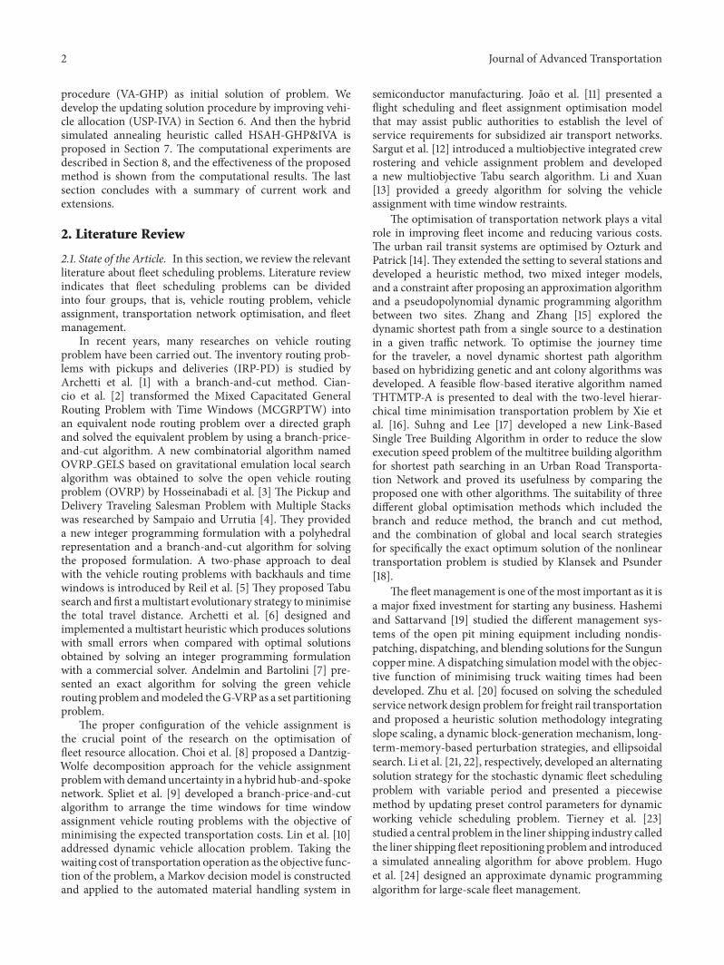
2 Journal of Advanced Transportation
procedure (VA-GHP) as initial solution of problem Wedevelop the updating solution procedure by improving vehi-cle allocation (USP-IVA) in Section 6 And then the hybridsimulated annealing heuristic called HSAH-GHPampIVA isproposed in Section 7 The computational experiments aredescribed in Section 8 and the effectiveness of the proposedmethod is shown from the computational results The lastsection concludes with a summary of current work andextensions
2 Literature Review
21 State of the Article In this section we review the relevantliterature about fleet scheduling problems Literature reviewindicates that fleet scheduling problems can be dividedinto four groups that is vehicle routing problem vehicleassignment transportation network optimisation and fleetmanagement
In recent years many researches on vehicle routingproblem have been carried out The inventory routing prob-lems with pickups and deliveries (IRP-PD) is studied byArchetti et al [1] with a branch-and-cut method Cian-cio et al [2] transformed the Mixed Capacitated GeneralRouting Problem with Time Windows (MCGRPTW) intoan equivalent node routing problem over a directed graphand solved the equivalent problem by using a branch-price-and-cut algorithm A new combinatorial algorithm namedOVRP GELS based on gravitational emulation local searchalgorithm was obtained to solve the open vehicle routingproblem (OVRP) by Hosseinabadi et al [3] The Pickup andDelivery Traveling Salesman Problem with Multiple Stackswas researched by Sampaio and Urrutia [4] They provideda new integer programming formulation with a polyhedralrepresentation and a branch-and-cut algorithm for solvingthe proposed formulation A two-phase approach to dealwith the vehicle routing problems with backhauls and timewindows is introduced by Reil et al [5] They proposed Tabusearch and first amultistart evolutionary strategy tominimisethe total travel distance Archetti et al [6] designed andimplemented a multistart heuristic which produces solutionswith small errors when compared with optimal solutionsobtained by solving an integer programming formulationwith a commercial solver Andelmin and Bartolini [7] pre-sented an exact algorithm for solving the green vehiclerouting problem andmodeled theG-VRP as a set partitioningproblem
The proper configuration of the vehicle assignment isthe crucial point of the research on the optimisation offleet resource allocation Choi et al [8] proposed a Dantzig-Wolfe decomposition approach for the vehicle assignmentproblemwith demanduncertainty in a hybrid hub-and-spokenetwork Spliet et al [9] developed a branch-price-and-cutalgorithm to arrange the time windows for time windowassignment vehicle routing problems with the objective ofminimising the expected transportation costs Lin et al [10]addressed dynamic vehicle allocation problem Taking thewaiting cost of transportation operation as the objective func-tion of the problem a Markov decision model is constructedand applied to the automated material handling system in
semiconductor manufacturing Joao et al [11] presented aflight scheduling and fleet assignment optimisation modelthat may assist public authorities to establish the level ofservice requirements for subsidized air transport networksSargut et al [12] introduced a multiobjective integrated crewrostering and vehicle assignment problem and developeda new multiobjective Tabu search algorithm Li and Xuan[13] provided a greedy algorithm for solving the vehicleassignment with time window restraints
The optimisation of transportation network plays a vitalrole in improving fleet income and reducing various costsThe urban rail transit systems are optimised by Ozturk andPatrick [14]They extended the setting to several stations anddeveloped a heuristic method two mixed integer modelsand a constraint after proposing an approximation algorithmand a pseudopolynomial dynamic programming algorithmbetween two sites Zhang and Zhang [15] explored thedynamic shortest path from a single source to a destinationin a given traffic network To optimise the journey timefor the traveler a novel dynamic shortest path algorithmbased on hybridizing genetic and ant colony algorithms wasdeveloped A feasible flow-based iterative algorithm namedTHTMTP-A is presented to deal with the two-level hierar-chical time minimisation transportation problem by Xie etal [16] Suhng and Lee [17] developed a new Link-BasedSingle Tree Building Algorithm in order to reduce the slowexecution speed problem of the multitree building algorithmfor shortest path searching in an Urban Road Transporta-tion Network and proved its usefulness by comparing theproposed one with other algorithms The suitability of threedifferent global optimisation methods which included thebranch and reduce method the branch and cut methodand the combination of global and local search strategiesfor specifically the exact optimum solution of the nonlineartransportation problem is studied by Klansek and Psunder[18]
The fleet management is one of themost important as it isa major fixed investment for starting any business Hashemiand Sattarvand [19] studied the different management sys-tems of the open pit mining equipment including nondis-patching dispatching and blending solutions for the Sunguncoppermine A dispatching simulationmodel with the objec-tive function of minimising truck waiting times had beendeveloped Zhu et al [20] focused on solving the scheduledservice network design problem for freight rail transportationand proposed a heuristic solution methodology integratingslope scaling a dynamic block-generation mechanism long-term-memory-based perturbation strategies and ellipsoidalsearch Li et al [21 22] respectively developed an alternatingsolution strategy for the stochastic dynamic fleet schedulingproblem with variable period and presented a piecewisemethod by updating preset control parameters for dynamicworking vehicle scheduling problem Tierney et al [23]studied a central problem in the liner shipping industry calledthe liner shipping fleet repositioning problem and introduceda simulated annealing algorithm for above problem Hugoet al [24] designed an approximate dynamic programmingalgorithm for large-scale fleet management
Journal of Advanced Transportation 3
22 Contributions Overall the objectives of this researchare twofold The first objective is to develop a mathematicalmodel of MHFS-FSD In the proposed model the matrixformulation denoting vehicle allocation scheme is exploredaccording to the characteristic of this problem The secondobjective is to propose an efficient methodology for solvingthe model Specifically the contributions of this paper are asfollows
(1) We develop the mixed integer programming model(MIP) This model discusses the integration of vehi-cles allocation and fleet sizing decisions consideringthe vehicle routing of multiple vehicle types Par-ticular vehicle type is assigned to some particulartransport routing according to the classification ofvehicles The matching of vehicle type and transportroute is given According to the characteristic of thisproblem the matrix formulation denoting vehicleallocation scheme is provided
(2) According to the specific structure of the mixedinteger programming model the approach of gener-ating vehicle allocation scheme with greedy heuristicprocedure (VA-GHP) as initial solution of problemis presented On the basis of the initial solution gen-erated by VA-GHP approach the USP-IVA methodto update the initial solution is developed and thenincorporating VA-GHP and USP-IVA into simulatedannealing algorithm a novel heuristic called HSAH-GHPampIVA is proposed
(3) To evaluate the performance of the heuristics pro-posed we generated randomly three sets of probleminstances with different size of freight terminal andtime periods considering different number of vehi-cles types Three sets of experiments are oriented toevaluate the performances of the hybrid simulatedannealing heuristic The results show that the pro-posed heuristic is able to obtain reasonably goodsolutions in short CPU times
3 Problem Description and Analysis
This section describes the problem of scheduling a heteroge-neous fleet of various vehicles over time to serve a set of loadswith fleet sizing decisions We make a brief overview of somefoundational concepts and analysis of the problem
31 Problem Description The freight transportation schedul-ing frequently aims to obtain appropriate capacity of trans-portation systems discover the potential of fleets of vehicleswhich circulate on networks and improve transportationefficiency by arranging daily transportation production rea-sonably organising vehicles flow adjustment scientificallyand making plans for loading and unloading operations intheir destination terminal of the networks efficiently
This paper discusses the integration of vehicles allocationand fleet sizing decisions considering the vehicle routingof multiple vehicle types Let 119866(119873 119864) represent the freighttransport network where 119873 is a set of freight terminal and
E represents the set of the movement of vehicles betweena pair of freight terminal We assume that time is dividedinto a set of discrete time periods 119867 = ℎ | ℎ = 1 119870where K is the length of the planning horizon and ℎ is thetime period All transitions require multiperiod travel timesLet 119905119894119895 be the travel time from 119894 to 119895 119894 119895 isin 119873 The traveltime between any pair of terminals is different length of timeperiod and integermultiple of one time periodThe operatorsof transportation systems manage a heterogeneous fleet ofvarious vehicles We define the set of classification of vehiclesas119882 = 1 sdot sdot sdot 119875 Particular vehicle type is assigned to someparticular vehicle routing according to the classification ofvehicles The matching of vehicle type and vehicle routingis given The use of operation vehicles will generate fixedexpenses such as vehicle leasing and daily maintenanceIt is crucial to decide the size of various vehicle typesreasonably
To maximise total profits over a given horizon theproblem is to optimise the fleet sizing and make the vehicleutilisation decision in view of the profit derived frommovinga load from terminal 119894 to terminal j denoted as 120572119908119894119895 the costof moving an empty vehicle from terminal 119894 to terminal 119895denoted as 120573119908119894119895 the fixed costs of owning or leasing a type ofvehicles denoted as 120574119908 and vehicle routing of vehicle typesdenoted as 120587119908 Figure 1 displays a snapshot of dynamic space-time network for fleet scheduling with multiperiod traveltimes
32 Understanding Vehicle Allocation between Pairs of Ter-minals A fleet of vehicles must be assigned to loads thathave the effect of moving the vehicle from one terminal tothe next The operator of the fleet must either assign eachvehicle to a requested loaded movement or move it empty toanother terminal to pick up a requested loadedmovement orto hold it in the same terminal until the next time period Sothe allocation problem of loaded vehicle and empty vehiclearises
Serving loads results in the relocation of vehiclesDemands request a vehicle to be available in a specificterminal on a specific time period to carry the load to a givendestination terminal Each load must be served by a vehicleLoaded movement will generate revenue So the loadedvehicle assignment is the basis of the vehicle allocation
The load for movements between various terminals isoften imbalanced and this implies the need for redistributionof empty vehicles over the transport network from terminalsat which they have become idle to terminals at which they canbe reused It is important to manage empty vehicle flows intransport network The loads create requirements for emptyvehicleThe arrivals of loaded vehicle flow create the suppliesof empties available for repositioning
Vehicle allocation has significant effects on the vehicledistribution or utilisation decision and then effects on capac-ity and efficiency of transport network
33 Understanding Heterogeneous Fleet of Vehicles Due tothe huge transport networks the large amount of loads andcomplex transport route conditions many conflicts will arisebetween homogeneous fleet of vehicles and heterogeneity
4 Journal of Advanced Transportation
Time periodKh h+1 h+2
Freight terminal 1
1
Freight terminal i
Freight terminal j
Freight terminal k
Freight terminal A
ℎ
Figure 1 Dynamic space-time network for fleet scheduling with multiperiod travel times
transport demands when freight transport schemes are car-ried out A homogeneous fleet with single vehicle type meansinefficiency in satisfying the diverse transport demandWhenthe operators manage a homogeneous fleet the vehicle short-age and idleness may occur synchronously The worseningtrend of vehicle utilisation is also possible to appear sothat transport efficiency is reduced and transport cost isenhanced Instead of homogeneous fleet with substitution ofsingle vehicle types for different types of transport demandssetting up heterogeneous fleets of vehicles is an effectivestrategy to eliminate the above unreasonable phenomenaoptimise the vehicle allocation and enhance the efficiency ofvehicle utilisation
Meanwhile the fleet size decisions are significant toimprove the freight carry capacity of fleet The insufficientvehicles seriously affect the implementation of transportwork If the number of available vehicles is not enough tomeet transport demand the penalty cost for unmet demandwill generate On the other hand the oversized supply of fleetfar more than the transport demand causes a large number ofvehicles to be idle
34 Understanding Vehicle Routing for Particular VehicleTypes Many works have assumed a homogeneous fleetof vehicles But most problems in practice have multiplevehicle types with limited substitution In this paper weextend the methodology to handle heterogeneous fleets ofvehicles with different vehicle types for different transportrouting
The two stage freight transport network is comprised offreight supply location as origin terminal and freight demandlocation as destination terminal In practical considerationsthe route from any supply location to demand locationcannot always be used to carry freight due to limited vehicletypes transport routing condition transport routing external
1
3
4
6
2A
5
1
3
4
6
2A
5
Figure 2 The vehicle routing of multiple vehicle types
environment and so on The specific reasons can be diverseas follows
(1) Some transport routes cannot be used by some specificvehicle type due to carry capacity of the road
(2) Some specific vehicle types are not allowed to travelon certain transport routes due to physical condition of theroad versus maintenance condition of vehicles
(3) Due to inexistence of supply location and demandlocation for freight exchange some transport routes disap-pear
An illustration of the vehicle routing of multiple vehicletypes is shown in Figure 2
Because some specific vehicle types are only allowed totravel on certain transport routes we use 120587 as the matchingmatrix such that 120587119908119894119895 = 1 if 119908 types of vehicle can be assignedto movement from terminal 119894 to 119895 and 120587119908119894119895 = 0 otherwise Wepresent the notation formore clearly expressing thematchingmatrix here119873 is the set of freight terminal in the freight transportnetwork Define 119873 = 1 sdot sdot sdot 119860 where A is the number offreight terminal119882 is the set of vehicle types in the heterogeneous fleetDefine 119882 = 1 sdot sdot sdot 119875 where 119875 is the total number ofavailable vehicles of various types
Journal of Advanced Transportation 5
119879 is thematrix of travel time of vehicles set between a pairof freight terminal We have
119879 =[[[[[[[[[[[[
0 sdot sdot sdot 1199051119895 sdot sdot sdot 1199051119860 1199051198941 sdot sdot sdot 119905119894119895 sdot sdot sdot 119905119894119860 1199051198601 sdot sdot sdot 119905119860119895 sdot sdot sdot 0
]]]]]]]]]]]]
forall119894 119895 isin 119873 (1)
120587 is the matrix of vehicle routing for certain vehicle typeThe matrix can be expressed by 120587 = 120587119908 | 119908 = 1 sdot sdot sdot 119875 Theparameter 120587119908 is used to represent practical situations wherevehicle type 119908 can be allowed to transport load on certainroutes Correspondingly we denote that
120587119908 =[[[[[[[[[[[[
12058711990811 sdot sdot sdot 1205871199081119895 sdot sdot sdot 1205871199081119860 1205871199081198941 sdot sdot sdot 120587119908119894119895 sdot sdot sdot 120587119908119894119860 1205871199081198601 sdot sdot sdot 120587119908119860119895 sdot sdot sdot 120587119908119860119860
]]]]]]]]]]]]
120587119908119894119895=
0 if vehicle type 119908 can move from terminal 119894 to 1198951 otherwise
forall119894 119895 isin 119873 119908 isin 119882
(2)
4 Mathematical Formulation
In this section we define the notation and formulate mul-tistage heterogeneous fleet scheduling with fleet sizing deci-sions (MHFS-FSD) as a mixed integer programming model
In the following we describe the model parameters andvariables used to model the MHFS-FSD
41 Model Parameters The parameters are needed todescribe the problem119905119894119895 is the travel time moving from origin 119894 to destination 119895and is the integer multiple of the scheduling time period120587119908119894119895 is the parameter for representing whether or notvehicle type119908 can be allowed to carry freight along transportrouting (119894 119895) The value of 120587119908119894119895 is 1 if the 119908 types of vehicle cancarry freight from the terminal 119894 to the terminal 119895 otherwisethe value is 0 forall119908 isin 119882 and forall119894 119895 isin 119873119902ℎ119894119895 is the set of loads with origin 119894 and destination 119895 havingℎ as a feasible departure forallℎ isin 119867 forall119894 119895 isin 119873120572119894119895 is the profits generated by a unit load being dispatchedfrom terminal 119894 to terminal 119895 forall119908 isin 119882 forall119894 119895 isin 119873120573119908119894119895 is the cost of 119908 type vehicle being repositioned emptyfrom terminal 119894 to terminal 119895 forall119908 isin 119882 forall119894 119895 isin 119873120574119908 is the purchase or lease cost for the 119908 type of vehicleforall119908 isin 119882120582119908 is the loading capacity of119908 type vehicle forall119908 isin 119882 Thatis to say it is the amount of loads which can be serviced byone 119908 type vehicle119911119908119894119905 is the number of available vehicle of119908 type at terminal119894 in time period t forall119908 isin 119882 forall119894 isin 119873
42Model Variables Thedecision variables of themathemat-ical model are119909ℎ119908119894119895 is the number of 119908 type of loaded vehicles fromterminal 119894 to terminal 119895 at time period ℎ forall119894 119895 isin 119873 ℎ isin 119867119910ℎ119908119894119895 is the number of 119908 type of empty vehicles fromterminal 119894 to terminal 119895 at time period ℎ forall119894 119895 isin 119873 ℎ isin 119867119911119908 is the number for available vehicle of 119908 type
43 Mathematical Models The mathematical models formultistage heterogeneous fleet scheduling with fleet sizingdecisions (MHFS-FSD) are given by
max 119865 (119909 119910 119911) = sum119908isin119882
( 119870sumℎ=1
sum119894isin119873
sum119895isin119873
(120572119894119895 sdotmin119902ℎ119894119895 sum119908isin119882
120582119908119909ℎ119908119894119895 minus 120573119908119894119895119909ℎ119908119894119895 minus 120573119908119894119895119910ℎ119908119894119895 ) minus 120574119908119911119908) (3)
119904119905 sum119895isin119873
(119909ℎ119908119894119895 + 119910ℎ119908119894119895 ) 120587119908119894119895 = 119911ℎ119908119894 forall119894 isin 119873 forallℎ isin 119867 forall119908 isin 119882 (4)
sum119908isin119882
120582119908119909ℎ119908119894119895 le 119902ℎ119894119895 forall119894 119895 isin 119873 forallℎ isin 119867 (5)
sum119894isin119873
(119909(ℎminus119905119894119895)119908119894119895 + 119910(ℎminus119905119894119895)119908119894119895 ) 120587119908119894119895 = 119911ℎ119908119895 forall119895 isin 119873 forallℎ isin 119867 forall119908 isin 119882 (6)
sum119894isin119873
119911ℎ119908119894 = 119911119908 forallℎ isin 119867 (7)
119909ℎ119908119894119895 ge 0 119910ℎ119908119894119895 ge 0 119911119908 ge 0 integer forall119894 119895 isin 119873 forallℎ isin 119867 forall119908 isin 119882 (8)
6 Journal of Advanced Transportation
The MHFS-FSD model belongs to a mixed integer pro-gramming model (MIP) The objective function (3) aims tomaximise the total profit generated by the fleet schedulingscheme during the whole planning horizon Constraint (4)denotes the number of dispatching loaded vehicles andempty vehicles are determined by supplies of vehicles in timeperiod Constraint (5) ensures that the number of loadedvehicle cannot exceed available requirements of all loads ineach terminal at each time period Constraint (6) denotesupdating equation for total supply of vehicle of various typesConstraint (7) shows having flow conservation of vehicle ineach type Finally constraint (8) defines the range of decisionvariables constraints
As an NP problem using traditional method for solvingMHFS-FSDmodel is difficult and inefficient A novel heuris-tic method is considered to solve this problem
5 Generating Initial Solution with VA-GHP
According to the characteristic of this problem the matrixformulation denoting vehicle allocation scheme is providedAnd then the approach of generating vehicle allocationscheme with greedy heuristic procedure as initial solution ofproblem is presented
51 Matrix Formulation of Vehicle Allocation The solution ofMHFS-FSD model represents the vehicle allocation schemeThe solution is expressed as two stage structureThe first termin the solution is matrix formulation of loaded vehicle dis-patching scheme The second term is the matrix formulationof empty vehicle reposition scheme
(1) e Matrix Formulation of Loaded Vehicle DispatchingScheme The first section of the solution is used to representthe loaded vehicle dispatching scheme of carrying freightfrom the origin terminal to the destination terminal Thissection is formulated as the matrix form which has 119860 rowsandA columns Each component in row and row intersectionof the matrix indicates the number of 119908 type loaded vehiclesfrom origin terminal to destination terminal The allocationscheme of loaded vehicle is written as the following formula
119909119908 =[[[[[[[[[[[[
11990911990811 sdot sdot sdot 1199091199081119895 sdot sdot sdot 1199091199081119860 1199091199081198941 sdot sdot sdot 119909119908119894119895 sdot sdot sdot 119909119908119894119860 1199091199081198601 sdot sdot sdot 119909119908119860119895 sdot sdot sdot 119909119908119860119860
]]]]]]]]]]]]
119908 isin 119882 (9)
(2) e Matrix Formulation of Empty Vehicle RepositionScheme The second section of the solution is used to denotethe empty vehicle reposition scheme of vehiclemoving emptyfrom the origin terminal to the destination terminal Thissection is also formulated as the matrix form which has119860 rows and 119860 columns Each component in row and rowintersection of the matrix expresses the number of 119908 typeempty vehicles from origin terminal to destination terminal
The allocation scheme of loaded vehicle is expressed as thefollowing formula
119910119908 =[[[[[[[[[[[[
11991011990811 sdot sdot sdot 1199101199081119895 sdot sdot sdot 1199101199081119860 1199101199081198941 sdot sdot sdot 119910119908119894119895 sdot sdot sdot 119910119908119894119860 1199101199081198601 sdot sdot sdot 119910119908119860119895 sdot sdot sdot 119910119908119860119860
]]]]]]]]]]]]
119908 isin 119882 (10)
52 Greedy Heuristic Procedure to Generate Vehicle AllocationScheme According to the fundamental principles of priori-tising to consider the vehicle types with large load capacityand transport routing with large carry capacity the greedyheuristic procedure is presented to generate vehicle allocationscheme We name this approach as vehicle allocation withgreedy heuristic procedure (VA-GHP) An overview of theframework of VA-GHP is explained as follows
Stage 1 (set of vehicle types selection sequence) Accordingto the vehicle distribution 119911ℎ119908119894 in terminal 119894 at ℎ time periodthe set of vehicle types selection sequence 119882ℎ119894 is obtainedwith ranking the vehicle types in descending order by loadingcapacity 120582119908 We denote 120575 as serial number of the vehicle typein this set and 120575 as the total quantity of available vehicle typesThus119882ℎ119894 has the form of
119882ℎ119894 = 119908ℎ119894 (120575) | 119908ℎ119894 (120575) = 119908 119908 isin 119882 120575 = 1 sdot sdot sdot 120575 (11)
Stage 2 (set of fleet size selection sequence) Let119885ℎ119894 be the setof fleet size selection sequence According to the set of vehicletypes selection sequence119882ℎ119894 we can express 119885ℎ119894 as
119885ℎ119894 = 119911ℎ119894 (120575) | 119911ℎ119894 (120575) = 119911ℎ119908119894 119908 isin 119882ℎ119894 120575 = 1 sdot sdot sdot 120575 (12)
Stage 3 (set of transport routing selection sequence) Werandomly choose the terminal 119894 from the set of freightterminal and compute the revenue 120572119894119895119902ℎ119894119895 created by loadedvehicle dispatched from origin 119894 to any available destination119895 We rank the transport routing in order of the revenuefrom high to low and the set of transport routing selectionsequence 119878ℎ119894 can be given We use 120585 to denote the serialnumber of transport routing in this set and the total numberof transport routing is represented as 120585ℎ119894 Here 119878ℎ119894 is written as
119878ℎ119894 = 119904ℎ119894 (120585) | 119904ℎ119894 (120585) = (119894 119895) 119895 isin 119873 120585 = 1 sdot sdot sdot 120585ℎ119894 (13)
The set of transport routing in terminal i at h time periodis described in Figure 3
Stage 4 (loaded vehicles dispatching scheme)
119878tep 41 (loaded vehicles dispatching scheme of transportrouting) The transport routing 119904ℎ119894 (120585) is selected in arrangedorder from the set of transport routing selection sequence
Journal of Advanced Transportation 7
h
Revenue
Routing
Descending
Terminal j
Terminal j
Terminal i
Terminal j
Terminal j
ℎ ℎ ℎ ℎ
sℎi (1)
sℎi (1)
sℎi ()
sℎi () sℎi (
)
sℎi ()
sℎi ()
sℎi ()
ij qℎij
ij qℎij
ij qℎij
ij qℎij
Figure 3 A diagram of the set of transport routing selection sequence
119878ℎ119894 According to the vehicle routing matrix 120587119908 for certainvehicle type the available vehicle types 119908ℎ119894 (120575) allowed totravel on the transport routing 119904ℎ119894 (120585) are chosen from thevehicle type selection sequence 119882ℎ119894 And the fleet size 119911ℎ119894 (120575)of corresponding vehicle types is determined from fleet sizeselection sequence 119885ℎ119894 We use the formula (14) to computeloaded vehicles dispatching scheme
119909ℎ120575119894 (120585) = minlceil119902ℎ119894 (120585)120582120575 rceil 119911ℎ119894 (120575) (14)
119878tep 42 (adjusting available loads number and available fleetsize for transport routing) (1) If there are lceil119902ℎ119894 (120585)120582120575rceil ge 119911ℎ119894 (120575)then 119909ℎ120575119894 (120585) = 119911ℎ119894 (120575) Besides let 119902ℎ119894 (120585) = 119902ℎ119894 (120585) minus 120582120575119911ℎ119894 (120575) and119911ℎ119894 (120575) = 0 turn to 119878tep 43
(2) If there are lceil119902ℎ119894 (120585)120582120575rceil le 119911ℎ119894 (120575) then 119909ℎ120575119894 (120585) =lceil119902ℎ119894 (120585)120582120575rceil Besides let 119902ℎ119894 (120585) = 0 and 119911ℎ119894 (120575) = 119911ℎ119894 (120575) minuslceil119902ℎ119894 (120585)120582120575rceil turn to 119878tep 44119878tep 43 (updating three selection sequence sets)
(1) Updating the Set of Transport Routing Selection SequenceAccording to available updated loads number 119902ℎ119894 (120585) therevenue of transport routingwith an origin terminal i is recal-culated The set of transport routing selection sequence 119878ℎ119894is updated with ranking the transport routing in descendingorder of the revenue 120572119894119895119902ℎ119894 (120585) The new set 119878ℎ119894 is expressed asfollows
119878ℎ119894 = 119904ℎ119894 (120585) | 119904ℎ119894 (120585) = (119894 119895) 119895 isin 119873 120585 = 1 sdot sdot sdot 120585ℎ119894 (15)
(2) Updating the Set of Vehicle Types Selection SequenceRemoving the vehicle types 119908ℎ119894 (120575) that have been used up
from vehicle selection sequence set119882ℎ119894 the new set of vehicletype selection sequence119882ℎ119894 can be given by
119882ℎ119894 = 119882ℎ119894 minus 119908ℎ119894 (120575)= 119908ℎ119894 (120575) | 119908ℎ119894 (120575) = 119908ℎ119894 (120575) 120575 = 120575 + 1 sdot sdot sdot 120575 (16)
(3)Updating the Set of Fleet Size Selection Sequence Removingthe fleet size 119911ℎ119894 (120575) of the vehicle types 119908ℎ119894 (120575) from fleet sizeselection sequence set 119885ℎ119894 the new set of fleet size selectionsequence 119885ℎ119894 can be given by
119885ℎ119894 = 119885ℎ119894 minus 119911ℎ119894 (120575)= 119911ℎ119894 (120575) | 119911ℎ119894 (120575) = 119911ℎ119894 (120575) 120575 = 120575 + 1 sdot sdot sdot 120575 (17)
119878tep 44 (updating two selection sequence sets)
(1) Updating the Set of Transport Routing Selection SequenceThe new set of transport routing selection sequence 119878ℎ119894is given with removing the transport routing 119904ℎ119894 (120585) fromtransport routing selection sequence 119878ℎ119894 The new set 119878ℎ119894 isexpressed as follows
119878ℎ119894 = 119878ℎ119894 minus 119904ℎ119894 (120585)= 119904ℎ119894 (120585) | 119904ℎ119894 (120585) = 119904ℎ119894 (120585) 120585 = 120585 + 1 sdot sdot sdot 120585ℎ119894 (18)
(2)Updating the Set of Fleet Sizing Selection SequenceThenewset of fleet size selection sequence119885ℎ119894 is obtained by updatingthe corresponding fleet size 119911ℎ119894 (120575) of vehicle type119908ℎ119894 (120575) in the
8 Journal of Advanced Transportation
fleet size selection sequence set119885ℎ119894 The new set119885ℎ119894 is denotedas
119885ℎ119894 = 119911ℎ119894 (120575) | 119911ℎ119894 (120575) = 119911ℎ119894 (120575) minus lceil119902ℎ119894 (120585)120582120575 rceil 119911ℎ119894 (120575 + 1) = 119911ℎ119894 (120575 + 1) 120575 = 120575 sdot sdot sdot 120575
(19)
Stage 5 (empty vehicle reposition scheme) We can obtain theloaded vehicles dispatching scheme 119909(ℎ+1minus119905119894119895)119908119894119895 by the proce-dure described in Stage 4 Substituting them into equationsum119894isin119873 119909(ℎ+1minus119905119894119895)119908119894119895 120587119908119894119895 = ℎ+1119908119895 the vehicles distribution ℎ+1119908119895can be obtained at terminal j at time period ℎ + 1 Andaccording to the load number 119902ℎ+1119894119895 at time period ℎ+1 emptyvehicle reposition scheme 119910ℎ119908119894119895 can be obtained
119878tep 51 (calculating the number of loads waiting to bearranged)Thenumber of loadswaiting to be arranged at eachfreight terminal 119902ℎ+1119895 is computed by the following formula
119902ℎ+1119895 = sum119896isin119873
119902ℎ+1119895119896 minus sum119908isin119882
120582119908ℎ+1119908119895 (20)
119878tep 52 (set of freight terminal selected sequence with lack ofempty vehicle) For the freight terminal where the number ofload waiting to be arranged 119902ℎ+1119895 is nonpositive it means thatthere are empty vehicles enough not to continue to call theempty vehicles Following the abovementioned principlesthe freight terminals with lack of empty vehicle are rankedin descending order of the revenues sum119896isin119873 120572119895119896119902ℎ+1119895119896 The set offreight terminal selected sequence with lack of empty vehicle119869ℎ+1 is formed We denote 120590 as the serial number of freightterminalwith lack of empty vehicle in this set 119869ℎ+1 and as thetotal quantity of freight terminal with lack of empty vehicleSo the new set 119869ℎ+1 can be expressed in the form by
119869ℎ+1 = 119895 (120590) | 119895 (120590) = 119895 119895 isin 119873 120590 = 1 sdot sdot sdot (21)
119878tep 53 (set of empty vehicles shortage amount selectedsequence) We count the shortage amount of freight terminalwith lack of empty vehicle in the set 119869ℎ+1 Further the setof empty vehicles shortage amount selected sequence 119876ℎ+1119895 isobtained and is denoted as 119876ℎ+1119895 = 119902ℎ+1119895 119895 isin 119869119878tep 54 (set of freight terminal selected sequence for dis-patching empty vehicle) The destination terminal j is suc-cessively taken out from the set of freight terminal selectedsequence with lack of empty vehicle 119869ℎ+1 Then according tothe vehicle routing matrix 120587119908 the origin terminal 119894 that has alinkwith destination terminal 119895 is taken out And ranking theorigin terminal 119894 in ascending order of the distance the setof freight terminal selected sequence for dispatching emptyvehicle 119868ℎ119895 is formed We denote 120579 as the serial number offreight terminal for dispatching empty vehicle in this set 119868ℎ119895and as the total quantity of freight terminal for dispatching
empty vehicle So the new set 119868ℎ119895 can be expressed in the formby
119868ℎ119895 = 119894 (120579) | 120587119908119894(120579)119895 = 1 119894 (120579) isin 119873119908 isin 119882 119895 isin 119869ℎ+1 120579= 1 sdot sdot sdot 120579ℎ119895 (22)
119878tep 55 (empty vehicle reposition scheme) We choosethe destination terminal j from the set of freight terminalselected sequence with lack of empty vehicle 119869ℎ+1 and theorigin terminal 119894(120579) from the corresponding set of freightterminal selected sequence for dispatching empty vehicle119868ℎ119895 In accordance with vehicle distribution 119885ℎ119894(120579) at freightterminal for dispatching empty vehicle 119894(120579) and loads number119902ℎ+1119895 at freight terminal with lack of empty vehicle we makeuse of the principle of priority arranging large capacity vehicletypes to conduct the empty vehicle reposition as the followingformula
119910ℎ120575119895 (120579) = min[[[
119902ℎ+1119895120582120575 ]]] 119911ℎ119894(120579) (120575) 119894 isin 119868ℎ119895 (23)
(1) If there are lceil119902ℎ+1119895 120582120575rceil ge 119911ℎ119894(120579)(120575) then119910ℎ120575119895 (120579) = 119911ℎ119894(120579)(120575)Additionally let 119902ℎ+1119895 = 119902ℎ+1119895 minus 120582120575119911ℎ119894(120579)(120575) and 119911ℎ119894(120579)(120575) = 0 Ifthere are still some other vehicle types unarranged at freightterminal for dispatching empty vehicle 119894(120579) they are furtherlymade by using equation (23) Otherwise succeeding freightterminal 119894(120579) should be taken out from the set of freightterminal selected sequence for dispatching empty vehicle 119868ℎ119895
(2) If there are lceil119902ℎ+1119895 120582120575rceil le 119911ℎ119894(120579)(120575) then119910ℎ120575119895 (120579) = lceil119902ℎ+1119895 120582120575rceil Besides let 119902ℎ+1119895 = 0 and119911ℎ119894(120579)(120575) = 119911ℎ119894(120579)(120575)-lceil119902ℎ+1119895 120582120575rceil In addition next destinationstation j is taken out from set of freight terminal selectedsequence with lack of empty vehicle 119869ℎ+1Stage 6 (updating the vehicle distributions) We usesum119894isin119873(119909(ℎ+1minus119905119894119895)119908119894119895 +119910(ℎ+1minus119905119894119895)119908119894119895 )120587119908119894119895 = 119911ℎ+1119908119895 to count the vehicledistributions 119885ℎ+1119908119895 in ℎ period and return to 119878tage 1
The approach of vehicle allocation with greedy heuristicprocedure (VA-GHP) is shown in Figure 4
6 Updating Solution Procedure by ImprovingVehicle Allocation
In this section we develop a method to update the initialsolution generated by VA-GHP approach mentioned aboveWe name this method as updating solution procedure byimproving vehicle allocation at local terminal This methodis abbreviated as USP-IVA in order to facilitate problemstatement Specially the USP-IVA is composed of two sub-proceduresThe first is called updating solution by improvingloaded vehicle dispatching scheme at single terminal and isabbreviated as US-ILVD The second is denoted as updatingsolution by improving empty vehicle reposition scheme at
Journal of Advanced Transportation 9
helliphellip
The vehicle allocation at 1 time period The vehicle allocation at K time period
routing with origin terminal 1
The vehicle allocation at h time period
Loaded vehicles Dispatching scheme at freight terminal 1
Empty vehicle reposition scheme
Loaded vehicles Dispatching scheme at freight terminal A
with origin terminal 1
routing with origin terminal Awith origin terminal A
terminal j(1) for empty vehicle reposition
routing with destination terminal j(1)
x1w(1)1 (1)
xhw(1)1 (1)
x1w()1 (1)
xhw()1 (1)
x1w(1)1 (
11) ( 11)x1w( )
1
x1w(1)A (1) x1w( )
A (1)
xhw(1)A (1) xhw( )
A (1)
x1w(1)A (
1A) x1w( )
A ( 1A)
y1w(1)j(1)
(1) y1w()j(1) (1j(1))
yhw(1)j(1)
(1) yhw()j(1) (hj(1))
y1w(1)j()
(1) y1w()j()
(1j())
xhw(1)1 (
h1) ( h1)xhw( )
1
xhw(1)A (
hA) xhw( )
A ( hA)
yhw(1)j()
(1) yhw()j()
(hj())
xKw(1)1 (1) xKw()
1 (1) xKw(1)1 (K1 ) xKw( )
1 (K1 )
xKw(1)A (1) xKw( )
A (1) xKw(1)A (KA) xKw( )
A (KA)
yKw(1)j(1)
(1) yKw()j(1) (Kj(1)) yKw(1)
j()(1) yKw()
j()(Kj())
w() vehicle type arranged for 1st transport
w() vehicle type arranged for 1st transport
ℎj(1) number of transport routing with destination
w() vehicle type arranged for ℎj(1) th transport
ℎ1 number of transport routing with origin terminal 1w() vehicle type arranged for ℎ1 th transport routing
ℎA number of transport routing with origin terminal Aw() vehicle type arranged for ℎAth transport routing
ℎj() number of transport routing with destinationterminal j() for empty vehicle repositionvehicle type arranged for ℎj() th transportw()
routing with destination terminal j()
Figure 4 Loaded vehicles dispatching and empty vehicle reposition scheme with greedy heuristic procedure
single terminal and is abbreviated as US-IEVR An overviewof the framework of US-ILVD and US-IEVR is explained inSections 61 and 62
61 Updating Solution by Improving Loaded Vehicle Dis-patching Scheme at Single Terminal It is not suitable togenerate vehicle allocation scheme by the principle of priorityarrangement for large load capacity vehicle types with VA-GHP approach for all freight terminals In consideration ofthese disadvantages we develop the solution improvementprocedure called US-ILVD based on the initial solution Theconcrete procedure of US-ILVD is as follows
Stage 1 (selecting the time period and freight terminal) Thetime period and freight terminal are selected randomly fromthe initial vehicle allocation scheme generated by VA-GHPand denoted as 119894∘ ℎ∘ | 119894∘ isin 119873 ℎ∘ isin 119867Stage 2 (updating loaded vehicle dispatching scheme ofspecific freight terminal and time period) 119878tep 21 (adjustingthe set of vehicle types selection sequence) According to thevehicle distribution 119911ℎ∘ 119908
119894∘in terminal 119894∘ at ℎ∘ time period the
new set of vehicle types selection sequence 1006704119882ℎ∘119894∘ is obtainedwith ranking the vehicle types in random order We denote 120575
as serial number of the vehicle type in this new set and 120575 asthe total quantity of available vehicle types Thus 1006704119882ℎ∘119894∘ can berecorded as
1006704119882ℎ∘119894∘ = 1006704119908ℎ∘119894∘ (120575) | 1006704119908ℎ∘119894∘ (120575) = 119908119908 isin 119882 120575 = 1 sdot sdot sdot 120575 (24)
119878tep 22 (adjusting loaded vehicles dispatching scheme oftransport routing)The transport routing 119904ℎ∘119894∘ (120585) is successivelychosen from the set of transport routing selection sequence119878ℎ∘119894∘ in order of the revenue from high to low According to thevehicle routing matrix 120587119908 the available vehicle types 1006704119908ℎ∘119894∘ (120575)allowed to travel on the transport routing 119904ℎ∘119894∘ (120585) is chosenfrom the new vehicle type selection sequence 1006704119882ℎ∘119894∘ And thefleet size 1006704119911ℎ∘119894∘ (120575) of corresponding vehicle types is obtainedfrom fleet size selection sequence 1006704119885ℎ∘119894∘ We use the formula(25) to ensure loaded vehicles dispatching scheme
119909ℎ∘120575119894∘ (120585) = minlceil119902ℎ∘119894∘ (120585)120582120575 rceil 1006704119911ℎ∘119894∘ (120575) (25)
119878tep 23 (adjusting available loads number and available fleetsize for transport routing) (1) If there are lceil119902ℎ∘119894∘ (120585)120582120575rceil ge
10 Journal of Advanced Transportation
adjusting loaded vehicle dispatching schemeat single freight terminal
Initial scheme of loaded vehicles dispatching at freight terminal i∘ in ℎ∘th time period
New scheme of loaded vehicles dispatching at freight terminal i∘ in ℎ∘th time period
(∘) vehicle type arranged for 1st transportrouting with origin terminal i∘
w(∘) vehicle type arranged for 1st transportrouting with origin terminal i∘
ℎ∘
i∘number of transport routing with origin terminal i∘
w(∘∘) vehicle type arranged for ℎ∘
i∘th transport routing
with origin terminal i∘
ℎ∘
i∘number of transport routing with origin terminal i∘
w( ∘∘)vehicle type arranged for ℎ∘
i∘th transport routing
with origin terminal i∘
xℎ∘w(1)
i∘(1) xℎ∘w(∘)
i∘(1)
xℎ∘w
w
(1)
i∘(1) xℎ∘w(∘)
i∘(1)
xℎ∘w(1)
i∘(ℎ
∘
i∘) xℎ∘w(∘∘ )
i∘(ℎ
∘
i∘)
xℎ∘ (1)
i∘(ℎ
∘
i∘) xℎ∘ww (∘∘ )
i∘(ℎ
∘
i∘)
Figure 5 Updating solutions by improving loaded vehicle dispatching scheme at single freight terminal
1006704119911ℎ∘119894∘ (120575) then 119909ℎ∘ 120575119894∘
(120585) = 1006704119911ℎ∘119894∘ (120575) Besides let 119902ℎ∘119894∘ (120585) = 119902ℎ∘119894∘ (120585) minus1205821205751006704119911ℎ∘119894∘ (120575) and 1006704119911ℎ∘119894∘ (120575) = 0 turn to 119878tep 24(2) If there are lceil119902ℎ∘119894∘ (120585)120582120575rceil le 1006704119911ℎ∘119894∘ (120575) then 119909ℎ∘120575
119894∘(120585) =lceil119902ℎ∘119894∘ (120585)120582120575rceil Besides let 119902ℎ∘119894∘ (120585) = 0 and 1006704119911ℎ∘119894∘ (120575) =1006704119911ℎ∘119894∘ (120575)-lceil119902ℎ∘119894∘ (120585)120582120575rceil turn to 119878tep 25
119878tep 24 (adjusting three selection sequence sets) We recountthe revenue 120572119894119895119902ℎ∘119894∘ (120585) for each transport routing The new set
of transport routing selection sequence 119878ℎ∘119894∘ is updated withranking the transport routing in descending order of therevenueThen after removing the vehicle types 1006704119908ℎ∘119894∘ (120575) used upfromvehicle selection sequence set 1006704119882ℎ∘119894∘ the new set of vehicle
type selection sequence 10067041006704119882ℎ∘119894∘ can be given Further removingthe fleet size 1006704119911ℎ∘119894∘ (120575) of the vehicle types 1006704119908ℎ∘119894∘ (120575) from fleet sizeselection sequence set 1006704119885ℎ∘119894∘ the new set of fleet size selection
sequence 10067041006704119885ℎ∘119894∘ can be obtained
119878tep 25 (adjusting two selection sequence sets) The newset of transport routing selection sequence 119878ℎ∘119894∘ is given afterremoving the transport routing 119904ℎ∘119894∘ (120585) from 119878ℎ∘119894∘ The new set of
fleet sizing selection sequence 10067041006704119885ℎ∘119894∘ is obtained after updatingthe corresponding fleet size 1006704119911ℎ∘119894∘ (120575) of vehicle type 1006704119908ℎ∘119894∘ (120575) inthe set of fleet sizing selection sequence 1006704119885ℎ∘119894∘ Stage 3 (determining loaded vehicle dispatching scheme ofother freight terminals) We work out the loaded vehicledispatching scheme at other freight terminals in the ℎ∘thtime period by the VA-GHP approach And then the vehicledistributions at each freight terminal in the (ℎ∘ + 1)th timeperiod are updated
Stage 4 (determining loaded vehicle dispatching and emptyvehicle reposition scheme for remaining time periods) Theloaded vehicle dispatching and empty vehicle repositionscheme is obtained by VA-GHP approach for remaining timeperiods after the ℎ∘th time period The updating solutionby improving loaded vehicle dispatching scheme at singleterminal is shown in Figure 5
62 Updating Solution by Improving Empty Vehicle RepositionScheme at Single Terminal On the basis of the improvedsolution obtained by US-ILVD secondary improvement pro-cedure called US-IEVR is further carried out The concreteprocedure of US-IEVR is as follows
Stage 1 (selecting the time period and freight terminal)The time period ℎlowast is selected randomly from planninghorizon And then the destination freight terminal 119895lowast ischosen randomly from freight terminal selected sequencewith lack of empty vehicle 119869ℎlowast They are denoted as 119895lowast ℎlowast |119895lowast isin 119873 ℎlowast isin 119867Stage 2 (adjusting the set of freight terminal selected sequencefor dispatching empty vehicle) According to the vehiclerouting matrix 120587119908 the origin terminal 119894lowast that has a linkwith destination terminal 119895lowast is taken out And ranking theorigin terminal 119894lowast in ascending order of the distance the setof freight terminal selected sequence for dispatching emptyvehicle 119868ℎlowastminus1119895lowast is obtainedWe denote 119894lowast(120579) as the serial numberof freight terminal for dispatching empty vehicle in this set119868ℎlowastminus1119895lowast
Stage 3 (adjusting empty vehicles reposition scheme) Wechoose successively the origin terminal 119894lowast(120579) from the cor-responding set of freight terminal selected sequence fordispatching empty vehicle 119868ℎlowastminus1119895lowast In accordance with vehicle
Journal of Advanced Transportation 11
Initial scheme of loaded vehicles dispatching at New scheme of loaded vehicles dispatching at
adjusting emptyvehicle repositionscheme at singlefreight terminal
freight terminal jlowast in ℎlowastth time period freight terminal jlowast in ℎlowastth time period
ℎlowast
jlowast number of transport routing with destinationterminminal jlowast for empty vehicle reposition
w(lowast) vehicle type arranged for ℎlowast
jlowast th transportrouting with destination terminal jlowast
w(lowast)
new vehicle type arranged for ℎlowast
jlowastthtransport routing with destination terminal jlowast
yℎlowastw(1)jlowast
(1) yℎlowastw(lowast )jlowast
(ℎlowast
jlowast ) yℎlowastw(1)jlowast
(1) yℎlowast (lowast )jlowast
(ℎlowast
jlowast )
w
Figure 6 Updating solutions by improving empty vehicle reposition scheme at single freight terminal
distribution 1006704119885ℎlowastminus1119894lowast(120579) at freight terminal for dispatching emptyvehicle 119894lowast(120579) and loads number 119902ℎlowast119895lowast at freight terminal withlack of empty vehicle 119895lowast we make use of the principle ofrandomly arranging vehicle types to generate the emptyvehicle reposition scheme as the following formula
119910ℎminus1120575119895lowast (120579) = min[[[[119902ℎlowast119895lowast120582120575 ]]]] 1006704119911ℎlowastminus1119894lowast(120579) (120575) 119894lowast isin 119868ℎlowastminus1119895lowast (26)
(1) If there are lceil119902ℎlowast119895 120582120575rceil ge 1006704119911ℎlowastminus1119894lowast(120579) (120575) 119910ℎminus1120575119895lowast (120579) = 1006704119911ℎlowastminus1119894lowast(120579) (120575)Additionally let 119902ℎlowast119895lowast = 119902ℎlowast119895lowast minus 1205821205751006704119911ℎlowastminus1119894lowast(120579) (120575) and 1006704119911ℎlowastminus1119894lowast(120579) (120575) =0 If there are still some other vehicle types in freightterminal for dispatching empty vehicle 119894lowast(120579) we generatefurther the empty vehicle reposition scheme by equation (26)Otherwise the next freight terminal 119894lowast(120579) is taken out fromthe set of freight terminal selected sequence for dispatchingempty vehicle 119868ℎlowastminus1119895lowast
(2) If there are lceil119902ℎlowast119895 120582120575rceil le 1006704119911ℎlowastminus1119894lowast(120579) (120575) 119910ℎlowastminus1120575119895lowast (120579) =lceil119902ℎlowast119895lowast 120582120575rceil Besides let 119902ℎlowast119895lowast = 0 and 1006704119911ℎlowastminus1119894lowast(120579) (120575) = 1006704119911ℎlowastminus1119894lowast(120579) (120575) minuslceil119902ℎlowast119895lowast 120582120575rceil And the procedures are stopped
Stage 4 (determining empty vehicle reposition scheme ofother freight terminals) We work out the empty vehiclereposition scheme at other freight terminals in the ℎlowastthtime period by the VA-GHP approach And then the vehicledistributions at each freight terminal in the (ℎlowast + 1)th timeperiod are updated
Stage 5 (determining loaded vehicle dispatching and emptyvehicle reposition scheme for remaining time periods) Theloaded vehicle dispatching and empty vehicle repositionscheme is obtained by VA-GHP approach for remaining timeperiods after the ℎlowastth time period The updating solution byimproving empty vehicle reposition scheme at single terminalis shown in Figure 6
7 Hybrid Simulated Annealing AlgorithmCombining VA-GHPampUSP-IVA
In this section we develop a hybrid simulated annealingheuristic to solve MHFS-FSD using the VA-GHP approach
and USP-IVAmethod described previously in Sections 5 and6 In this proposed algorithm we use the VA-GHP procedureto generate initial solutions and the USP-IVA procedureto improve the solutions We incorporate VA-GHP andUSP-IVA into simulated annealing algorithm So the hybridsimulated annealing heuristic is proposed The detailed stepsof hybrid simulated annealing heuristics (HSAH) are asfollows
71 Acceptance Measure of Solutions (1) Acceptance Measurefor US-ILVD Let 120595lowast = (119883ℎ 119884ℎ 119885ℎ) | ℎ = 1 sdot sdot sdot 119870 denotethe solution accepted currently and 120595(119894∘ ℎ∘)119880119878minus119868119871119881119863 = 120595lowast 997888rarr1006704119883ℎ∘119894∘ express the new solution obtained by US-ILVD of singleterminal (119894∘ ℎ∘) We let 119865+(119894∘ ℎ∘)119880119878minus119868119871119881119863 be the incremental cost asfollows
119865+(119894∘ ℎ∘)119880119878minus119868119871119881119863 = 119865 (120595(119894∘ℎ∘)119880119878minus119868119871119881119863) minus 119865 (120595lowast) (27)
The acceptance measure of new solution 120595(119894∘ℎ∘)119880119878minus119868119871119881119863 iswritten as follows
119875(120595(119894∘ ℎ∘)119880119878minus119868119871119881119863)
= 1 if 119865+(119894∘ ℎ∘)USminusILVD le 0exp(minus119865+(119894∘ ℎ∘)119880119878minus119868119871119881119863119905 ) if 119865+(119894∘ ℎ∘)USminusILVD gt 0
(28)
where 119875(120595(119894∘ℎ∘)119880119878minus119868119871119881119863) denotes the acceptance probability ofnew solution 120595(119894∘ ℎ∘)119880119878minus119868119871119881119863(2) AcceptanceMeasure for US-IEVR Let120595lowast = (119883ℎ 119884ℎ 119885ℎ) |ℎ = 1 sdot sdot sdot 119870 denote the solution accepted currently and120595(119895lowast ℎlowast)119880119878minus119868119864119881119877 = 120595lowast 997888rarr 1006704119884ℎlowast119895lowast express the solution obtained byUS-IEVR of single terminal (119895lowast ℎlowast) Let us define 119865+(119895lowast ℎlowast)119880119878minus119868119864119881119877as the incremental cost We have that
119865+(119895lowast ℎlowast)119880119878minus119868119864119881119877 = 119865 (120595(119895lowast ℎlowast)119880119878minus119868119864119881119877) minus 119865 (120595lowast) (29)
12 Journal of Advanced Transportation
We can form the acceptance measure of new solution120595(119895lowast ℎlowast)119880119878minus119868119864119881119877 as follows
119875(120595(119895lowast ℎlowast)119880119878minus119868119864119881119877)
=
1 if 119865+(119895lowast ℎlowast)119880119878minus119868119864119881119877 le 0exp(minus119865+(119895
lowast ℎlowast)
119880119878minus119868119864119881119877119905 ) if 119865+(119895lowast ℎlowast)119880119878minus119868119864119881119877 gt 0(30)
where 119875(120595(119895lowast ℎlowast)119880119878minus119868119864119881119877) is the acceptance probability of newsolution 120595(119895lowast ℎlowast)119880119878minus119868119864119881119877
72 Control Parameters of the Heuristics
(1) Initial Temperature Parameter 1199050 In order to return a highquality final solution at the end of the algorithm iterationwe must give a large enough value to 1199050 But the exorbitantinitial temperature can cause the sharp growth of CPU runtime so that makes the algorithm lose its feasibility So welet 1199050 = 2 times 119865(120595lowast) where 119865(120595lowast) is the objective functionvalue obtained by taking the vehicles allocation scheme 120595 =(1198831 1198841 1198851) (119883119870 119884119870 119885119870) into objective function ofMHFS-FSD model
(2) Termination Criterion Here we give a very small positivenumber 119905119891 as the termination temperature of hybrid sim-ulated annealing heuristics During the iterative procedureof the algorithm the temperature control parameter 119905 isgradually reduced When the temperature control parameter119905 is less than 119905119891 the algorithm will be terminated
(3) Attenuation Function of Temperature Control ParameterIn order to avoid overlong running times in each iterationthe decrement of temperature control parameter t shouldtake a small value Here we have the attenuation function oftemperature control parameter as follows
119905119896+1 = 120572 sdot 119905119896 119896 = 0 1 0 lt 120572 lt 1 (31)
where 119905119896 and 119905119896+1 are respectively the temperaturecontrol parameter in 119896th iteration and (119896 + 1)th iteration 120572 isthe attenuation coefficient and we assume 120572 to be 09
(4) Solution Transformation Times The acceptance proba-bility of new solution will reduce with the decrease of thetemperature control parameter 119905119896 Consequently solutiontransformation times 119871119896 should gradually increase whentemperature control parameter 119905119896 drops that is 119905119896 darr997904rArr 119871119896 uarrHere we have the dynamic solution transformation timesbased on algorithm iterative procedure
119871119896+1 = 120573 sdot 119871119896 119896 = 0 1 120573 gt 1 (32)
where 119871119896 and 119871119896+1 are respectively the solution trans-formation times in 119896th iteration and (119896 + 1)th iteration and120573 is the increasing rate We assume 120573 to be 11 and 1198710 to be anumber between 50sim100
Termination conditionYes
Counting solution transformation timesImplementing US- IEVR subprocedureImplementing US-ILVD subprocedure
No
setting
generating
obtaining
loop body
estimating
Implementing US-IVA procedure
Implementing GHP method
Initial vehicle allocation scheme
Control parameters of cooling schedule
Final solution
Iteration based on cooling schedule
Figure 7 Flow diagram of hybrid simulated annealing heuristics
73 Heuristic Procedure For illustration purpose the hybridsimulated annealing heuristic combining greedy heuris-tic procedure for initial solution and improving vehicleallocation for updating solution is abbreviated as HSAH-GHPampIMA Figure 7 depicts a flowchart of the hybridsimulated annealing heuristics The heuristic procedure canbe described as follows
Stage 1 (initial scheduling scheme generated by GHP) Let120595 = (1198831 1198841 1198851) (119883119870 119884119870 119885119870) denote the vehicleallocation scheme of whole planning horizon obtained byVA-GHP And then the objective function value 119865(120595) can beobtained by taking it into the objective function of MHFS-FSD model Besides we let 120595lowast = 120595Stage 2 (setting control parameters) We set the initial tem-perature 1199050 termination temperature 119905119891 attenuation coef-ficient of temperature control parameter 120572 initial solutiontransformation times 1198710 and increasing rate of solutiontransformation times 120573 And then let 119905 = 1199050 119871 = 1198710 turnto 119878tep 2Stage 3 (iteration based on cooling schedule)
119878tep 1 (measuring termination condition) In case 119905 gt 119905119891 thealgorithm procedure turns to 119878tep 2 Otherwise move to 119878tep4
119878tep 2 (implementing US-IVA procedure) Let 119894 = 1119878tep 21 (implementing US-ILVD subprocedure) Afterchoosing randomly the adjustment freight terminal andtime period (119894∘ ℎ∘) we use US-ILVD procedure to improvesolution120595lowast so that the new solution120595(119894∘ℎ∘)119880119878minus119868119871119881119863 is obtainedThe
Journal of Advanced Transportation 13
119865+(119894∘ ℎ∘)119880119878minus119868119871119881119863 value is calculated by equation (27) If 119865+(119894∘ ℎ∘)119880119878minus119868119871119881119863 le0we accept the new solution and let 120595lowast = 120595(119894∘ ℎ∘)119880119878minus119868119871119881119863 Ifa random number R between 0 and 1 is generated andexp(minus119865+(119894∘ ℎ∘)119880119878minus119868119871119881119863119905) ge R we accept the new solution andlet 120595lowast = 120595(119894∘ ℎ∘)119880119878minus119868119871119881119863 Otherwise we reject to accept the newsolution and 120595lowast remain unchanged The procedure goes to119878tep 22119878tep 22 (implementing US- IEVR subprocedure) Afterchoosing randomly the adjustment freight terminal andtime period (119895lowast ℎlowast) we use US-IEVR procedure to improvesolution120595lowast so that the new solution120595(119895lowast ℎlowast)119880119878minus119868119864119881119877 is obtainedThe119865+(119895lowast ℎlowast)119880119878minus119868119864119881119877 value is calculated by equation (29) If 119865+(119895lowast ℎlowast)119880119878minus119868119864119881119877 le0we accept the new solution and let 120595lowast = 120595(119895lowast ℎlowast)119880119878minus119868119864119881119877 Ifa random number R between 0 and 1 is generated andexp(minus119865+(119895lowast ℎlowast)119880119878minus119868119864119881119877119905) ge R we accept the new solution andlet 120595lowast = 120595(119895lowast ℎlowast)119880119878minus119868119864119881119877 Otherwise we reject to accept the newsolution and 120595lowast remain unchanged The procedure goes to119878tep 23119878tep 23 (counting solution transformation times) Let 119894 = 119894 +1 If there is 119894 le 119871 turn to 119878tep 21 else go to 119878tep 24119878tep 24 (adjusting temperature and solution transformationtimes) Let 119905 = 119905 times 120572 and 119871 = 119871 times 120573 and go to 119878tep 1Stage 4 (obtaining final solution) When the terminationcriterion is met the final solution 120595lowast can be obtained
8 Numerical Experiments
In this section we try to evaluate the quality of the hybridsimulated annealing algorithm combining VA-GHPampUSP-IVA proposed in previous section to solve the MHFS-FSD interms of traditional measure such as objective function andexecution time The scenarios for MHFS-FSD are describedin Section 81 and three sets of experiments are devised to testthe effectiveness of the hybrid simulated annealing algorithmproposed Section 82 reports the numerical results
81 Scenario Settings of the Experiments To design theexperiments scheme the scenarios settings need to be firstlyset up This section describes the data used in the numericaltesting of the models We generated the dataset based onthe freight enterprise in Henan Province China Howeverthe data have some inconsistencies caused by multiple typesof the vehicles differences in financial accounting system ofvarious corporations and so on Therefore the data has to becleaned
Here we chose a certain range from 40RMB to 60RMBper load as the revenue of loaded movement between variousfreight terminals The loading capacity of various type vehi-cles is allowed the certain range from 20 units to 30 units pervehicle The cost of empty reposition is allowed the certainrange from 200RMB to 300 RMB per vehicleWe use the costrange from 2000RMB to 3000 RMB per vehicles as purchaseor lease cost of various vehicles
To evaluate the performance of the heuristics proposedwe generate randomly three sets of problem instances withdifferent size of freight terminal and time periods con-sidering different number of vehicles types Three sets ofexperiments are oriented to compare the performances of thehybrid simulated annealing algorithmwith the CPLEX solverand VA-GHP approach
In the first set of contrast experiment there are theheterogeneous fleet with three types of vehicles and five timeperiods The number of the freight terminal is from 5 to10 In the second set of contrast experiment there are theheterogeneous fleet with five types of vehicles and ten timeperiods The number of the freight terminal is from 11 to20 In the third set of contrast experiment there are theheterogeneous fleet with ten types of vehicles and thirty timeperiods The number of the freight terminal is from 21 to50
The test work has been done using a computer withIntel i5-5200CPU (22GHz)The hybrid simulated annealingalgorithm combining VA-GHPampUSP-IVA has been coded inMicrosoft Visual C++
82 Performance Evaluation In this section the compu-tational experiments are performed using three methodsto solve the MHFS-FSD model HSAH program GHPapproach and CPLEX solver And we use two measures toevaluate the performance The first one is the OPT which isthe value of the objective function obtained by the CPLEXsolver GHP approach and HSAH program OPT as one ofthe major criteria in assessing the performance of the HSAHGHP and CPLEX represents the profit generated by revenuesfor dispatching loaded vehicles repositioning empty vehiclesand ownership costs for owning vehicle in planning horizonThe second measure of performance is the CUP time to runCPLEX solver the GHP approach and HSAH program forMHFS-FSD model We aim at quantifying the benefits ofthe proposed method in two aspects (1) the efficiency of theproposed method executed with no time limit imposed and(2) the efficiency of the proposed method executed with timelimit imposed
(1) Measure of Performance with No CPUTime Limit ImposedIn this section we focus on the numerical studies onthe performance of GHP approach HSAH program andCPLEX solver executed with no CPU time limit imposedWe compare the performance of these three methods intwo aspects solution quality and computational efficiencyIn Tables 1ndash3 we present the results obtained by solvingrandomly generated MHFS-FSD problems We compare thesolutions obtained by solving theMHFS-FSD problems usingGHP approach HSAH program and CPLEX solver
CPLEX solver is executed with no time limit imposedThe parameters used for the HSAH are as follows The initialtemperature is set by 1199050 = 2 times 119865(120595lowast) where 119865(120595lowast) isthe objective function value obtained by taking the initialsolution solved with VA-IGP into objective function ofMHFS-FSD model The termination temperature is set to 1The attenuation coefficient of temperature control parameteris assumed to be 09 The initial solution transformation
14 Journal of Advanced Transportation
Table 1 Performance for CPLEX GHP and HSAH applied to small size problem with no time limit imposed
Problem size (freightterminal times vehicle types timestime period)
CPLEX GHP HSAHOS CPU time OFV CPU time RAT GAP OFV CPU time RAT GAP
(RMB) (second) (RMB) (second) () (second) (RMB) (second) () (second)5 times 3 times 5 219586 2145 165894 136 2445 2009 199473 336 916 18096 times 3 times 5 225465 2357 184759 157 1805 2200 209484 375 709 19827 times 3 times 5 230187 3562 163028 139 2918 3423 190583 366 1721 31968 times 3 times 5 246586 2483 190324 216 2282 2267 224756 456 885 20279 times 3 times 5 250829 3212 186206 258 2576 2954 208573 504 1685 270810 times 3 times 5 276585 3145 201478 231 2716 2914 235859 556 1472 2589
Table 2 Performance for CPLEX GHP and HSAH applied to medium size problem with no time limit imposed
Problem size (freightterminal times vehicle types timestime period)
CPLEX GHP HSAHOS CPU time OFV CPU time RAT GAP OFV CPU time RAT GAP
(RMB) (second) (RMB) (second) () (second) (RMB) (second) () (second)11 times 5 times 10 727865 3895 512034 897 2965 2998 708543 1967 265 192812 times 5 times 10 767289 3972 536401 914 3009 3058 741478 1834 336 213813 times 5 times 10 876537 4057 641963 1034 2676 3023 835317 2099 470 195814 times 5 times 10 782685 4123 541069 1135 3087 2988 729294 2203 682 192015 times 5 times 10 813858 4342 571648 738 2976 3604 787625 1778 322 256416 times 5 times 10 882385 4518 642917 1125 2713 3393 837674 2296 507 222217 times 5 times 10 926048 4469 702541 1009 2414 3460 892573 2142 361 232718 times 5 times 10 949874 4671 731529 852 2299 3819 932074 1921 187 275019 times 5 times 10 998375 4826 768359 784 2304 4042 948927 1874 495 295220 times 5 times 10 1010948 5137 763542 1043 2447 4094 978375 2106 322 3031
Table 3 Performance for CPLEX GHP and HSAH applied to large size problem with no time limit imposed
Problem size (freightterminal times vehicle types timestime period)
CPLEX GHP HSAHOS CPU time OFV CPU time RAT GAP OFV CPU time RAT GAP
(RMB) (second) (RMB) (second) () (second) (RMB) (second) () (second)21 times 10 times 30 3641457 10466 3162419 3517 1316 6949 3592236 6315 135 415122 times 10 times 30 3960247 11537 3375864 3632 1476 7905 3890437 6542 176 499523 times 10 times 30 4093746 12413 3392618 3891 1713 8522 3962476 6910 321 550324 times 10 times 30 4172590 13069 3521607 4125 1560 8944 4063582 7196 261 587325 times 10 times 30 4395799 13881 3862453 4347 1213 9534 4298741 7679 221 620226 times 10 times 30 4673825 14497 3971641 4438 1502 10059 4495476 7790 382 670727 times 10 times 30 4691793 15338 4071358 5034 1322 10304 4586179 8391 225 694728 times 10 times 30 4762133 15924 4193062 5367 1195 10557 4703167 8642 124 728229 times 10 times 30 4792619 16403 4083017 5763 1481 10640 4698731 8996 196 740730 times 10 times 30 4821617 17316 4262843 5986 1159 11330 4803164 9043 038 827331 times 10 times 30 4865329 17961 4228019 6026 1310 11935 4829316 9325 074 863632 times 10 times 30 4887691 18742 4353762 6479 1092 12263 4796317 9667 187 907533 times 10 times 30 4963720 19240 4464907 7124 1005 12116 4850691 10432 228 880834 times 10 times 30 5120379 19896 4526143 7268 1161 12628 5006479 11325 222 857135 times 10 times 30 5436826 20465 4593011 7793 1552 12672 5267984 11646 311 881936 times 10 times 30 5761844 21653 4612938 8524 1994 13129 5706914 12542 095 911137 times 10 times 30 5839764 22212 4685714 8370 1976 13842 5784639 12756 094 945638 times 10 times 30 6032875 23022 4703519 9543 2204 13479 5859217 13248 288 977439 times 10 times 30 6361448 23995 4794808 9894 2463 14101 6263941 13961 153 1003440 times 10 times 30 6673280 25564 4862714 10326 2713 15238 6612476 14432 091 1113241 times 10 times 30 6805218 28265 5182913 10581 2384 17684 6569031 15041 347 1322442 times 10 times 30 6961760 29733 5403917 11298 2238 18435 6795213 15754 239 1397943 times 10 times 30 7134752 32056 5632051 11867 2106 20189 6948217 16145 261 1591144 times 10 times 30 7446389 33605 5789830 10563 2225 23042 7164206 16532 379 1707345 times 10 times 30 7623796 35866 5913517 12194 2243 23672 7501286 17418 161 1844846 times 10 times 30 7853219 38882 6242683 12347 2051 26535 7632689 18136 281 2074647 times 10 times 30 7905256 41696 6590263 11964 1663 29732 7693618 18568 268 2312848 times 10 times 30 8134962 42753 6832657 13247 1601 29506 8047603 19436 107 2331749 times 10 times 30 8416732 44536 7207149 17172 1437 27364 8267798 20662 177 2387450 times 10 times 30 8601795 46791 7421678 15368 1372 31423 8396419 21647 239 25144
Journal of Advanced Transportation 15
5 6 7 8 9 1015
25
2
Freight terminal
HSAH
CPLEX
GHP
3 times 105
Tota
l pro
fit (R
MB)
(a) Objective function value
6 7 8 9 10Freight terminal
HSAH
GHP
RAT
()
5
10
15
30
25
20
(b) Deviation rate
350
250
150
50
5 6 7 8 9 10Freight terminal
HSAH
CPLEX
GHP
CPU
tim
e (s)
(c) CPU running time
300
250
200
1505 6 7 8 9 10
Freight terminal
HSAH
GHP
GA
P (s
)
(d) CPU time gap
Figure 8 Results of comparison for small size problem
frequency is allowed 80 The increasing rate of the solutiontransformation frequency is assumed to be 11
In order to facilitate problem analysis we introduce twoanalytical indicators The first denoted as RAT representsthe deviation rate from the optimal solution Let OFV bethe objective function value with GHP approach and HSAHprogram And let OS be optimal solution obtained withCPLEX solver The RAT is calculated by
RAT = (OS minusOFV)OS
(33)
The second is the CPU time gap denoted as GAP It iscalculated by the difference betweenCUP time of running theHSAH program or GHP approach and that of CPLEX solverThe CPU times of running HSAH program GHP approachand CPLEX solver are respectively denoted as CPUTHSAHCPUGHP and CPUTCPLEX The GAP is calculated by
GAP = (CPUTCPLEX minus CPUTHSAH)GAP = (CPUTCPLEX minus CPUTGHP) (34)
The performance of small size problem is shown inTable 1 Here we have 6 test problems Each problemis respectively solved using the proposed GHP approachHSAH program and CPLEX solver For the small size
problem the performance of GHP and HSAH is not veryprominent when compared to CPLEX And the performanceof HSAH is better than GHP The deviations of GHP fromthe optimal solution are the range from 18 to 30 while thedeviations of HSAH from the optimal solution are the rangefrom 7 to 20 The CPU times to obtain the solutions arethe range from 336 s to 556 s forHSAH the range from 136 sto 231 s for GHP and the range from 2145 s to 3562 s forCPLEX The superiority of GHP and HSAH in computingtime can be shown distinctly The results of comparison aredisplayed in Figure 8
The performance of medium size problem is shown inTable 2 Here we have 10 test problems Each problem isrespectively solved using the proposed GHP HSAH andCPLEX For the medium size problem the GHP and HSAHperform well when compared to CPLEX The performanceof HSAH is prominent than GHP The deviations from theoptimal solution are reduced to a reasonable range from 2to 7 forHSAH and the deviations from the optimal solutionrange from 22 to 31 for GHP One obvious observation isthat the increase of CUP time to obtain the solutions usingCPLEX begins to appear a trend of acceleration But therising step of CPU times to obtain the solutions using GHPand HSAH increases is relatively flat So the superiority ofGHP and HSAH in computation time is very obvious Theperformance comparisons are shown in Figure 9
16 Journal of Advanced Transportation
12 14 16 18 20
6
10
8
9
7
5
CPLEX
HSAH
GHP
Freight terminal
Tota
l pro
fit (R
MB)
11times105
(a) Objective function value
10
30
12 14 16 18 20
20
GHP
HSAH
Freight terminal
RAT
()
(b) Deviation rate
100
200
300
400
12 20181614
500
CPLEX
HSAH
GHP
Freight terminal
CPU
tim
e (s)
(c) CPU running time
200
250
300
350
2012 14 16 18
400
GHP
HSAH
Freight terminal
GA
P (s
)
(d) CPU time gap
Figure 9 Results of comparison for medium size problem
The performance of large size problem is shown inTable 3 Here we have 30 test problems Each problem isrespectively solved using the proposed GHP HSAH andCPLEX For the large size problem performance of solvingthe problem using theGHP andHSAH ismore excellent thanthat of CPLEX The deviations from the optimal solution forHSAH are limited to a very small range within 4 while thedeviations from the optimal solution for the GHP are limitedto range within 30 But the CPU times for obtaining thesolutions using CPLEX solver increase in a sharp speed dueto the high memory requirements The superiority of GHPand HSAH in computation time is particularly obvious Theperformance comparisons are shown in Figure 10
(2) Measure of Performance with CPU Time Limit ImposedIn the experiment we test the performance of the HSAHprogram and CPLEX solver with CPU time limit imposedSince the performance of GHP approach is obviously inferiorto that of HSAS program GHP approach is no longer testedin the experiment Here the HSAS program is fully executedAnd let CPLEX solver be executed for the same CPU timeThen we compare the objective function value obtained bysolving the MHFS-FSD problems using HSAH program andCPLEX solver The tests are performed mainly in Tables 4ndash6
From above three sets of contrast tests the objectivefunction values obtained by HSAH program are significantly
better than those obtained by CPLEX solver with CPU timelimit imposed
In sum we can conclude that the HSAH is effective toobtain good solutions in relatively low run times for theMHFS-FSD The results obtained indicate the benefits ofusing HSAH helping MHFS-FSD to find better solutionsin reasonable short CPU times which are acceptable forpractical applications
9 Conclusions
The study described in this paper attempts to integratevehicles allocation and fleet sizing decisions considering thevehicle routing of multiple vehicle types We name the prob-lem as multistage heterogeneous fleet scheduling with fleetsizing decisions (MHFS-FSD) In this paper a mixed integerprogramming model has been developed for MHFS-FSD Asan NP problem using traditional method for solving MHFS-FSD model is difficult and inefficient A novel heuristic isconsidered to solve this problem
According to the characteristic of this problem thematrix formulation denoting vehicle allocation scheme isprovided The approach of generating vehicle allocationscheme with greedy heuristic procedure (VA-GHP) as initialsolution of problem is presented On the basis of the initialsolution generated by VA-GHP approach the USP-IVA
Journal of Advanced Transportation 17
Table 4 Results for HSAH and CPLEX applied to small size problem with time limit imposed
Problem size (freight terminal times vehicle types times time period) OFV (RMB) CPU time (second)CPLEX HSAH5 times 3 times 5 53817 199473 3366 times 3 times 5 57429 209484 3757 times 3 times 5 61437 190583 3668 times 3 times 5 68413 224756 4569 times 3 times 5 73076 208573 50410 times 3 times 5 78462 235859 556
Table 5 Results for HSAH and CPLEX applied to medium size problem with time limit imposed
Problem size (freight terminal times vehicle types times time period) OFV (RMB) CPU time (second)CPLEX HSAH11 times 5 times 10 493276 708543 196712 times 5 times 10 497625 741478 183413 times 5 times 10 513410 835317 209914 times 5 times 10 526683 729294 220315 times 5 times 10 525914 787625 177816 times 5 times 10 543728 837674 229617 times 5 times 10 562807 892573 214218 times 5 times 10 567436 932074 192119 times 5 times 10 573614 948927 187420 times 5 times 10 592460 978375 2106
Table 6 Results for HSAH and CPLEX applied to large size problem with time limit imposed
Problem size (freight terminal times vehicle types times time period) OFV (RMB) CPU time (second)CPLEX HSAH21 times 10 times 30 2561437 3592236 631522 times 10 times 30 2746308 3890437 654223 times 10 times 30 3012561 3962476 691024 times 10 times 30 3348021 4063582 719625 times 10 times 30 3585719 4298741 767926 times 10 times 30 3602476 4495476 779027 times 10 times 30 3680418 4586179 839128 times 10 times 30 3764292 4703167 864229 times 10 times 30 3791068 4698731 899630 times 10 times 30 3822516 4803164 904331 times 10 times 30 3849317 4829316 932532 times 10 times 30 3886203 4796317 966733 times 10 times 30 3965042 4850691 1043234 times 10 times 30 4002837 5006479 1132535 times 10 times 30 4125340 5267984 1164636 times 10 times 30 4196205 5706914 1254237 times 10 times 30 4273568 5784639 1275638 times 10 times 30 4305217 5859217 1324839 times 10 times 30 4362208 6263941 1396140 times 10 times 30 4385426 6612476 1443241 times 10 times 30 4412716 6569031 1504142 times 10 times 30 4472930 6795213 1575443 times 10 times 30 4502814 6948217 1614544 times 10 times 30 4575356 7164206 1653245 times 10 times 30 4598325 7501286 1741846 times 10 times 30 4620819 7632689 1813647 times 10 times 30 4673369 7693618 1856848 times 10 times 30 4702923 8047603 1943649 times 10 times 30 4785527 8267798 2066250 times 10 times 30 4832509 8396419 21647
18 Journal of Advanced Transportation
25 30 35 40 50
3
7
5
Tota
l pro
fit (R
MB)
Freight terminal
6
4
45
8
2
CPLEX
GHP
HSAH
9 times 106
(a) Objective function value
RAT
()
Freight terminal25 30 35 45
30
25
15
20
0
5
5040
10
HSAH
GHP
(b) Deviation rate
3
4
CPU
tim
e (s)
Freight terminal25 50403530 45
2
1
CPLEX HSAH
GHP
5times103
(c) CPU running time
05
1
15
2G
AP
(s)
Freight terminal5025 30 35 40 45
25
GHP
HSAH
3 times 103
(d) CPU time gap
Figure 10 Results of comparison for large size problem
method to update the initial solution is developed And thenincorporating VA-GHP and USP-IVA into simulated anneal-ing algorithm a novel heuristic called HSAH-GHPampIVA isproposed Finally we evaluate the performance of the hybridsimulated annealing heuristic in terms of traditional measuresuch as objective function and execution time The resultsshow that the proposed heuristic is able to obtain reasonablygood solutions in short CPU times
Future research can focus on new heuristics to solve theMHFS-FSD Another prospective research will be to extendthe model of MHFS-FSD by introducing further realisticaspects and relaxing hard constraints
Data Availability
The data used to support the findings of this study areavailable from the corresponding author upon request
Conflicts of Interest
The authors declare that there are no conflicts of interestregarding the publication of this paper
Acknowledgments
This research is supported by National Natural ScienceFoundation of China (Grant no U1604150 and U1804151)
References
[1] C Archetti M Christiansen and M Grazia Speranza ldquoInven-tory routing with pickups and deliveriesrdquo European Journal ofOperational Research vol 268 no 1 pp 314ndash324 2018
[2] C Ciancio D Lagana and F Vocaturo ldquoBranch-price-and-cutfor the mixed capacitated general routing problem with timewindowsrdquo European Journal of Operational Research vol 267no 1 pp 187ndash199 2018
[3] A A RHosseinabadi J Vahidi V E Balas and S SMirkamalildquoOVRP GELS solving open vehicle routing problem usingthe gravitational emulation local search algorithmrdquo NeuralComputing and Applications vol 29 no 10 pp 955ndash968 2018
[4] A H Sampaio and S Urrutia ldquoNew formulation and branch-and-cut algorithm for the pickup and delivery traveling sales-man problem with multiple stacksrdquo International Transactionsin Operational Research vol 24 no 1-2 pp 77ndash98 2017
[5] S Reil A Bortfeldt and L Monch ldquoHeuristics for vehiclerouting problems with backhauls time windows and 3Dloading constraintsrdquo European Journal of Operational Researchvol 266 no 3 pp 877ndash894 2018
[6] C Archetti M Savelsbergh and M G Speranza ldquoThe vehiclerouting problem with occasional driversrdquo European Journal ofOperational Research vol 254 no 2 pp 472ndash480 2016
[7] J Andelmin and E Bartolini ldquoAn exact algorithm for the greenvehicle routing problemrdquo Transportation Science vol 51 no 4pp 1288ndash1303 2017
Journal of Advanced Transportation 19
[8] J Choi C Lee and S Park ldquoDantzig-Wolfe decompositionapproach to the vehicle assignment problem with demanduncertainty in a hybrid hub-and-spoke networkrdquo Annals ofOperations Research vol 264 no 1-2 pp 57ndash87 2018
[9] R Spliet S Dabia and T Van Woensel ldquoThe time windowassignment vehicle routing problemwith time-dependent traveltimesrdquo Transportation Science vol 52 no 2 pp 261ndash276 2018
[10] J T Lin C H Wu and C W Huang ldquoDynamic vehicleallocation control for automated material handling systemin semiconductor manufacturingrdquo Computers and OperationsResearch vol 40 no 10 pp 2329ndash2339 2013
[11] P P Joao A Nicole and P A Antonio ldquoSocially-oriented flightscheduling and fleet assignment model with an application toNorwayrdquo Transportation Research Part B Methodological vol61 no 3 pp 17ndash32 2017
[12] F Z Sargut C Altuntas and D C Tulazoglu ldquoMulti-objectiveintegrated acyclic crew rostering and vehicle assignment prob-lem in public bus transportationrdquo OR Spectrum vol 39 no 4pp 1071ndash1096 2017
[13] B Li and H Xuan ldquoGreedy algorithm for the vehicle allocationproblemwith timewindowsrdquoOperations Research andManage-ment Science vol 22 no 2 pp 92ndash98 2013
[14] O Ozturk and J Patrick ldquoAn optimization model for freighttransport using urban rail transitrdquo European Journal of Oper-ational Research vol 267 no 3 pp 1110ndash1121 2018
[15] S Zhang and Y Zhang ldquoA hybrid genetic and ant colonyalgorithm for finding the shortest path in dynamic trafficnetworksrdquo Automatic Control and Computer Sciences vol 52no 1 pp 67ndash76 2018
[16] F Xie M M Butt and Z Li ldquoA feasible flow-based iterativealgorithm for the two-level hierarchical time minimizationtransportation problemrdquoComputersampOperations Research vol86 pp 124ndash139 2017
[17] B M Suhng and W Lee ldquoA new link-based single treebuilding algorithm for shortest path searching in an urban roadtransportation networkrdquo Journal of Electrical Engineering andTechnology vol 8 no 4 pp 889ndash898 2013
[18] U Klansek and M Psunder ldquoSolving the nonlinear transporta-tion problem by global optimizationrdquo Transport vol 25 no 3pp 314ndash324 2010
[19] A S Hashemi and J Sattarvand ldquoSimulation based investi-gation of different fleet management paradigms in open pitmines-a case study of Sungun copper minerdquo Archives of MiningSciences vol 60 no 1 pp 195ndash208 2015
[20] E Zhu T G Crainic and M Gendreau ldquoScheduled servicenetwork design for freight rail transportationrdquo OperationsResearch vol 62 no 2 pp 383ndash400 2014
[21] B Li and H Xuan ldquoAlternating solution strategies of bi-levelprogramming model for stochastic dynamic fleet schedulingproblem with variable period and storage propertiesrdquo Controland Decision vol 30 no 5 pp 807ndash814 2015
[22] B Li W Xu H Xuan and C Q Xu ldquoDynamic vehicle schedul-ing for working service network with dual demandsrdquo Journal ofAdvanced Transportation vol 2017 Article ID 7217309 13 pages2017
[23] K Tierney B Askelsdottir R M Jensen and D PisingerldquoSolving the liner shipping fleet repositioning problem withcargo flowsrdquo Transportation Science vol 49 no 3 pp 652ndash6742015
[24] P S Hugo D Jeff P G Abraham et al ldquoAn approximatedynamic programming algorithm for large-scale fleet manage-ment a case applicationrdquo Transportation Science vol 43 no 2pp 178ndash197 2009
International Journal of
AerospaceEngineeringHindawiwwwhindawicom Volume 2018
RoboticsJournal of
Hindawiwwwhindawicom Volume 2018
Hindawiwwwhindawicom Volume 2018
Active and Passive Electronic Components
VLSI Design
Hindawiwwwhindawicom Volume 2018
Hindawiwwwhindawicom Volume 2018
Shock and Vibration
Hindawiwwwhindawicom Volume 2018
Civil EngineeringAdvances in
Acoustics and VibrationAdvances in
Hindawiwwwhindawicom Volume 2018
Hindawiwwwhindawicom Volume 2018
Electrical and Computer Engineering
Journal of
Advances inOptoElectronics
Hindawiwwwhindawicom
Volume 2018
Hindawi Publishing Corporation httpwwwhindawicom Volume 2013Hindawiwwwhindawicom
The Scientific World Journal
Volume 2018
Control Scienceand Engineering
Journal of
Hindawiwwwhindawicom Volume 2018
Hindawiwwwhindawicom
Journal ofEngineeringVolume 2018
SensorsJournal of
Hindawiwwwhindawicom Volume 2018
International Journal of
RotatingMachinery
Hindawiwwwhindawicom Volume 2018
Modelling ampSimulationin EngineeringHindawiwwwhindawicom Volume 2018
Hindawiwwwhindawicom Volume 2018
Chemical EngineeringInternational Journal of Antennas and
Propagation
International Journal of
Hindawiwwwhindawicom Volume 2018
Hindawiwwwhindawicom Volume 2018
Navigation and Observation
International Journal of
Hindawi
wwwhindawicom Volume 2018
Advances in
Multimedia
Submit your manuscripts atwwwhindawicom
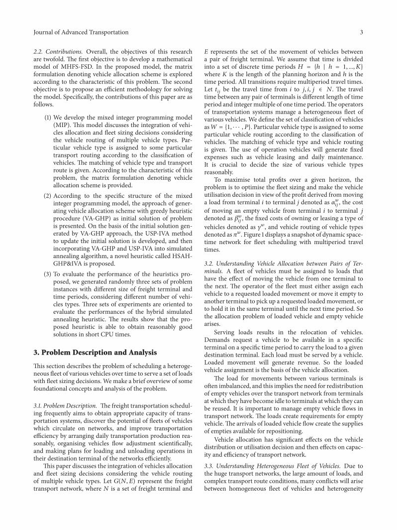
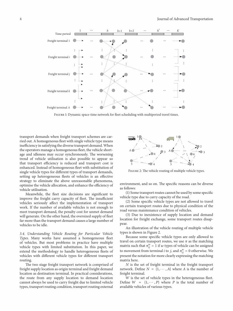
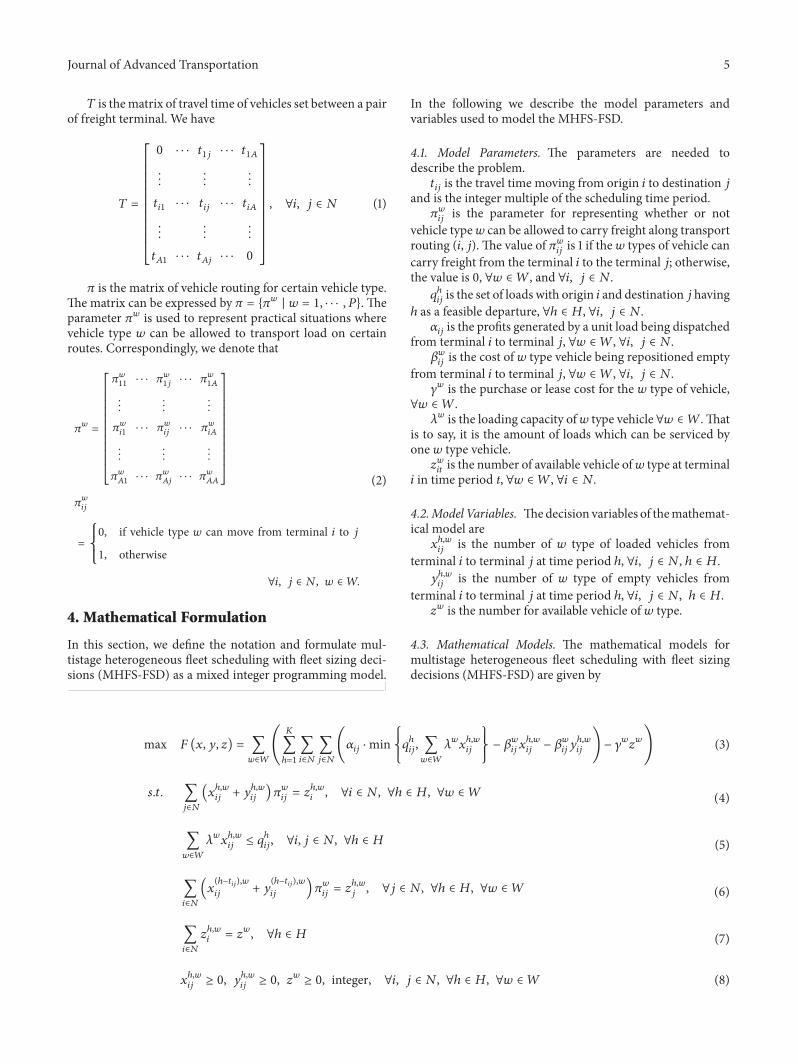
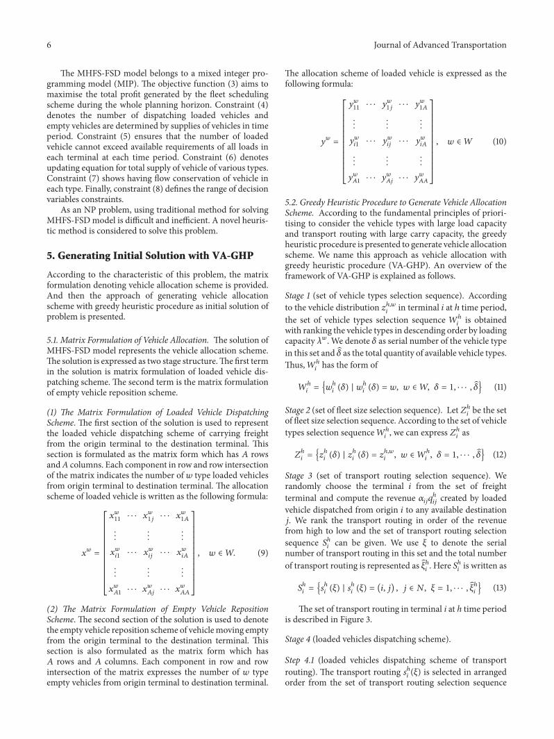
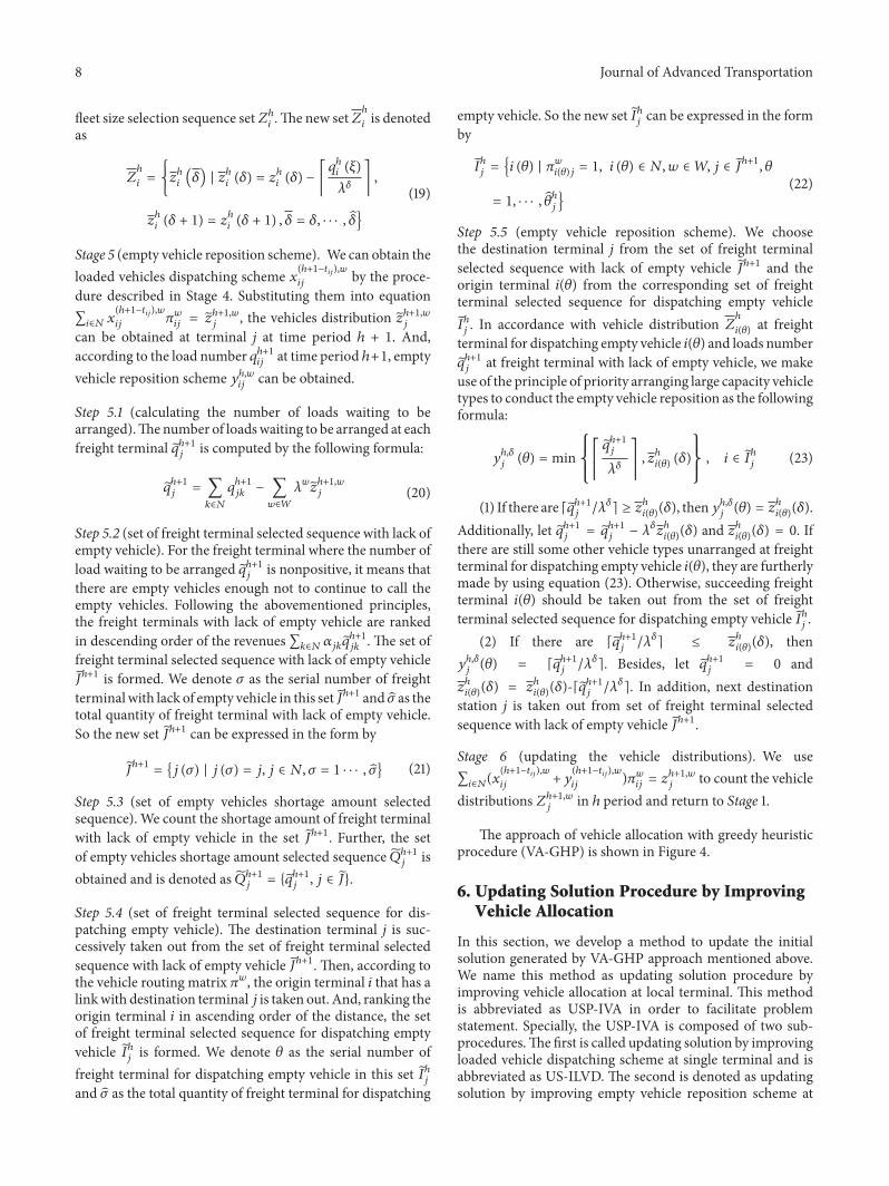
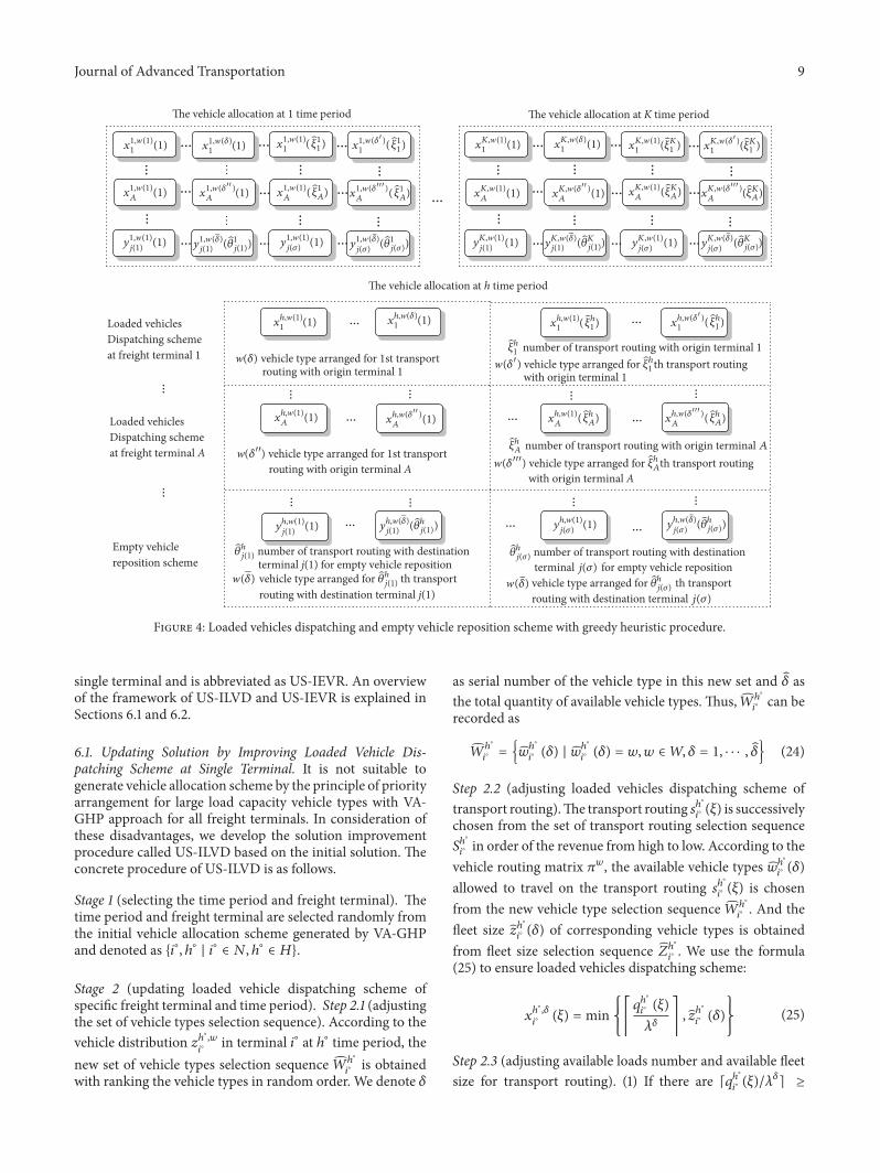
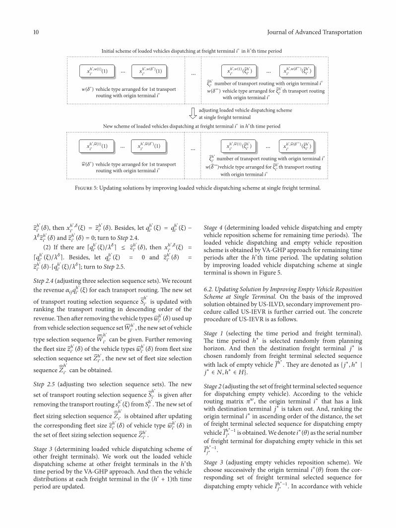
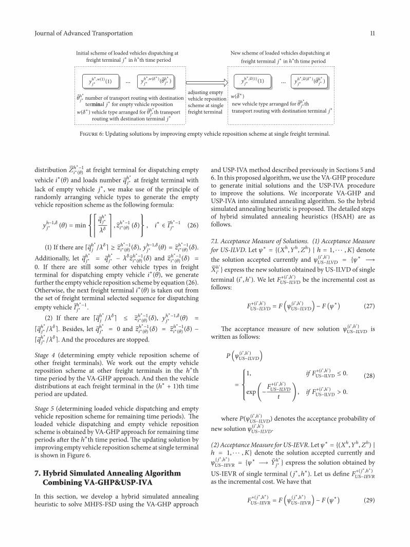
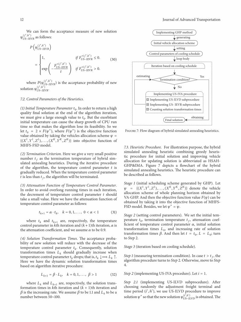
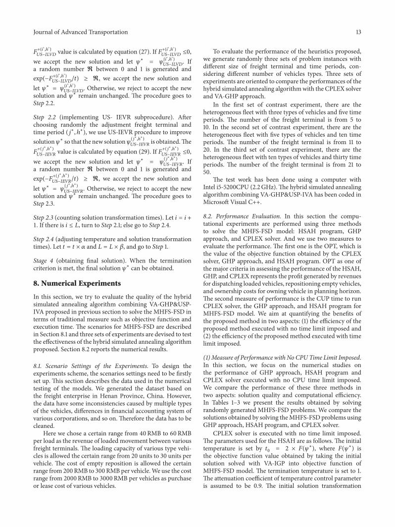
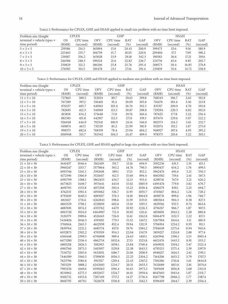
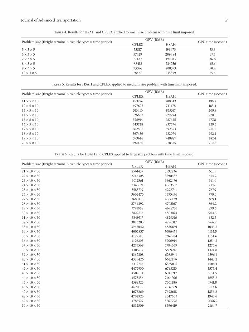
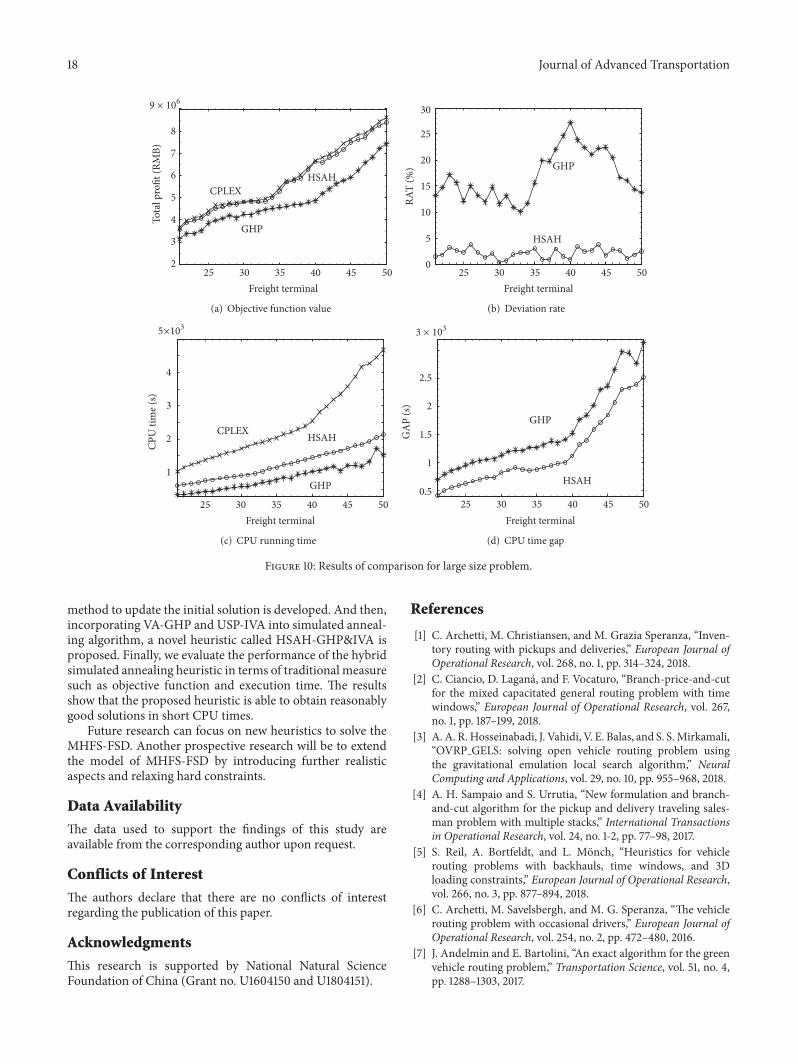

International Journal of
AerospaceEngineeringHindawiwwwhindawicom Volume 2018
RoboticsJournal of
Hindawiwwwhindawicom Volume 2018
Hindawiwwwhindawicom Volume 2018
Active and Passive Electronic Components
VLSI Design
Hindawiwwwhindawicom Volume 2018
Hindawiwwwhindawicom Volume 2018
Shock and Vibration
Hindawiwwwhindawicom Volume 2018
Civil EngineeringAdvances in
Acoustics and VibrationAdvances in
Hindawiwwwhindawicom Volume 2018
Hindawiwwwhindawicom Volume 2018
Electrical and Computer Engineering
Journal of
Advances inOptoElectronics
Hindawiwwwhindawicom
Volume 2018
Hindawi Publishing Corporation httpwwwhindawicom Volume 2013Hindawiwwwhindawicom
The Scientific World Journal
Volume 2018
Control Scienceand Engineering
Journal of
Hindawiwwwhindawicom Volume 2018
Hindawiwwwhindawicom
Journal ofEngineeringVolume 2018
SensorsJournal of
Hindawiwwwhindawicom Volume 2018
International Journal of
RotatingMachinery
Hindawiwwwhindawicom Volume 2018
Modelling ampSimulationin EngineeringHindawiwwwhindawicom Volume 2018
Hindawiwwwhindawicom Volume 2018
Chemical EngineeringInternational Journal of Antennas and
Propagation
International Journal of
Hindawiwwwhindawicom Volume 2018
Hindawiwwwhindawicom Volume 2018
Navigation and Observation
International Journal of
Hindawi
wwwhindawicom Volume 2018
Advances in
Multimedia
Submit your manuscripts atwwwhindawicom